Model-based visual feedback control for a hand-eye coordinated robotic system

P

1 Model-Based Visual Feedback Control for a Hand-Eve Coordinated

J

Robotic System

John T. Feddema, Sandia National Laboratories

C.S. George Lee, Purdue University 0. Robert Mitchell, University of Texas at Arlington

ensor integration is vital in flexible manufacturing workcells. Without sensors, manufacturing systems must control environments precisely and maintain exact knowledge of plant models. A change in a task or the

environment involves the time and expense of adjusting and recalibrating the system. With appropriate sensors, the system becomes flexible enough to compensate for such changes automatically. The reductions both in downtime for mis- aligned parts and in fixturing costs more than offset initial sensor costs.

Sensors allow robots to go beyond simple pick-and-place operations, enabling them to manipulate parts with uncertain characteristics and locations. Sensors for vision, force, range, and touch can eliminate the need to position parts exactly, thus minimizing workpiece fixturing. They can also verify assembly and gauge parts on line, thus eliminating the need for off-line inspection.

Vision sensors are especially helpful, and many industry systems currently use single-camera systems to locate parts. However, these systems are typically slow and inaccurate. In their normal mode of operation, they take a picture, analyze the image, extract position information from it, and move the robot accordingly. If the part moves unpredictably while the image is being analyzed, the robot will not “know” its new position.

To track randomly moving parts, a robot must have real-time vision feedback. This feedback, often called vision-guided servoing, gives the robot control system appropriate signals for mating the end-effector, or robot gripper, with the part.

There are many potential applications for this technology. These include precision part placement, arc welding, seam tracking, vehicle guidance, space structure control, and composite layout. However, implementation of vision-guided servoing requires solutions to several challenging problems. For example, effective

Using and differential, as

opposed to absolute, visual feedback, this flexible robot control

system tracks a moving object and guides the

robot gripper to it.

August 1992 001X-9162/92/0800-0021$03.00 IG 1992 IEEE 21

Camera B

- - - - - - 0 Tw 6 Workpiece

Camera B:

Ib- Ib rb -1 0 w... Pf, = s, F,-b (OTCb) T w P f ,

Figure 1. Coordinate frames in robot's workspace. The equations are used to de. termine the position of a feature point in the image planes for cameras A and B.

robot control implies a 10- to 100-millisecond vision cycle time (that is, the time required to analyze images and extract features from them). Providing this operational bandwidth with current off-the-shelf image processing equipment is difficult and requires sig- nificant reductions in the amount of image data. One way we can reduce data is to search small region-of-interest windows for a few salient image features. But how many and which features should we choose to control the robot's desired degrees of freedom.

Another problem is the variation in vision cycle time with image complexi- ty and size. This requires the system's control structure to accoumodate nonuniform sampling of the vision feedback. The resultingvariable delay makes discrete time analysis and control ex- tremely difficult, if not impossible. We need another means of control.

This article focuses on the integra-

tion of a single camera into a robotic system to control the relative position and orientation (that is, the pose) between the robot's end-effector and a moving part in real time. We consider only monocular vision techniques, as opposed to binocular (or stereo) vision techniques, because of current limita- tions in the speed of computer vision analysis. Our approach uses geometric models of both the part and the camera, as well as the extracted image features, to generate the appropriate robot control signals for tracking. We also use part and camera models during the teaching stage to predict important image features that will appear during task completion.

Problem statement Spatial relationships play an impor-

tant role in robotics. The relative pose

22

between a robot's end-effector and a workpiece tells us how close the robot is to contact with the workpiece (usually an eventual subgoal of a task). As human beings, we use the sense of sight to estimate the relative pose of objects with respect to our hands. Similarly, we would like to use computer vision to estimate the relative pose of the robot's gripper to a workpiece. The estimated pose could then be fed back into the robot controller where control adjust- ments could be made in the gripper's pose.

Correct camera placement is critical to hand-eye coordinated robotic motion. Human beings, for instance, position their heads closer to the object for a task such as threading a needle than they d o for tightening a large bolt. Sim- ilarly, the appropriate camera position relative to the robot's workspace de- pends on the precision of the task and the resolution of the camera. We will consider the camera in two positions: on the robot end-effector (camera A in Figure 1) or stationary with respect to the base coordinate frame of the robot (camera B in Figure 1).

To analyze the visual feedback problem, we must first look at the spatial relationships among four objects in Fig- ure I :

the robot's gripper, the robot's camera, the stationary camera, and a workpiece.

The position and orientation between the robot's end-effector, the cameras, and the part may be represented by 4 x 4 homogeneous transformations.' For example. the pose relationship of a workpiece w with respect to a fixed coordinate frame 0 is given by

where "R, is an orthonormal 3 x 3 rotation matrix, 0 is a 3 x 1 row vector of zeros, and "pW is a 3 x 1 position vector. The multiplication property of homogeneous transformations allows the pose of the workpiece with respect to the fixed frame 0 to also be expressed as a product of the homogeneous transform of the robot's end-effector with respect to the frame 0, "T,, and the homogeneous transform of the workpiece with respect to the robot's end-effector, eTw:

COMPUTER

=TW - O T, = o ~ c b c b ~ w Robot * control

end-effector frame

T, = "T, 'T,

lacatton Actual Robot robot

kinematics -

dynamics -

This property may also be used to describe the pose of the workpiece's features, f,, i = 1,. . . , m, with respect to the frame 0:

Estimated workpiece pose with respect

to camera 6

'T, =OT,"T,, for i = l , . . . ,m

- Location Feature Camera B

These features might include holes, edges, or corners on the workpiece. Ideally, the transformations of the features with respect to the workpiece, , T , , could be determined from a CAD model of the workpiece.

While homogeneous transformations correctly describe the relative pose in the Cartesian space between two objects, they do not describe the camera transformation from the three-dimensional Cartesian space into the two-dimensional image plane. Geometric optics are often used to model the mapping between a point in the Cartesian space and a point in the image plane. This mapping consists of two stages: a thin lens model of the perspective transformation, 'F, and a mapping into a two- dimensional plane caused by image sampling, ISr. For a lens perpendicular to the image plane, the transformation from the camera frame c to the image plane I can be written as

*TW determination - extraction -

or

optics <

w ' 5 , = iS,'Fc'P,

where 'p, is a 2 x 1 vector representing

image plane, w is a scalar scaling factor,

Absolute visual the (x, y ) position of the point in the feedback cl, and ay are the camera sampling fac- tors in pixels per millimeter, ('x,,, ' yo) is the focal center in pixels, f is the focal length of the camera in millimeters, and cp, is a 3 x 1 vector representing the (x, y , z ) position of the point with respect to the camera frame. Tsia2 presents more complex expressions for IS, and 'F, to account for the effects of blurring, lens distortion, and quantization.

Homogeneous transformations and the camera model make it possible to simulate the positions of the workpiece's features in the image plane of both cameras A and B. Figure 1 shows how to determine the (x, y ) position of a feature point i in both cameras' image coordinates, given the model of the workpiece ("pJ, its pose with respect to a fixed frame 0 (T,), camera A's pose with respect to the robot's end-effector (eTca), camera B's pose with respect to the fixed frame 0 ("TCb), the end-effector'spose with respect to the fixed frame 0 (OT,), and camera parameters (laSra,

Computer graphics use these types of equations extensively to display three-dimensional objects on a two-dimensional screen. However, for visual feedback control, we are interested in an inverse solution. That is, given the two-dimensional image positions of the workpiece's features, the model of the workpiece, the camera parameters, the pose of the robot's end-effector, and the pose of the cameras, what is the workpiece's pose with respect to the fixed frame O?

'"F,,, IbSrh, and 'hFch).

Computer vision has been used with robotic systems for quite some time. Early robot manufacturers did not offer an integrated vision system, so vision systems were usually loosely coupled into the robotic system as after-market add-ons. The long image processing time of these systems limited their use to locating stationary objects or parts moving at a fixed rate on a conveyor.

Figure 2 shows the position-based, look-and-move control structure used in most of these systems.'Typically, the vision system would take several sec- onds to locate a workpiece, after which it would send the robot control system the estimated pose of the workpiece with respect to a fixed coordinate frame. After the robot moved to the appropriate position, the vision system would take another "picture" and repeat the process.

Not only were the early vision systems slow, but they were also very limited in application. Even today, most monocular vision systems will only locate an object if it is on a plane perpendicular to the camera's focal axis at a fixed distance from the camera. The main reason for this is that the camera transformation reduces three-dimensional data to two-dimensional data. An exact inverse of this equation does not exist. Given the (x, y ) image position of a single point, it is impossible to determine the ( x , y , z ) position of the point in the 3D space. We can only determine

August 1992 23

the ray extending from the focal center on which the point lies. Fortunately. we can determine an object's pose from ihree or more image points if we know the spatial distances between these points (see thesidebar"Locati0n determination problem").

We would usually like the robot's end-effector to move to a point relative to the workpiece. Suppose this transformation is given by "T,. Assuming that we are using camera B, we will use the location-determination method discussed in the sidebar to denote the mea- sured object's pose by the homogeneous

transformation 'hT,. Then we determine the transformation of this desired end- effector pose with respect to the robot's base coordinates by premultiplying LhTU by "T,, and postmultiplying by "T,. Most robot systems will accept this resultant homogeneous transformation as an ac- ceptable command pose.

The same process could be performed with feature points with respect to camera A except the transformation 'IT,, will depend on the robot's current pose, (Te, and the camera's pose, LTca. Most robotic systems will accept robot move statements in terms of homogeneous

Location-determination problem

Fischler and Bolles' were among the first to solve the location-determination problem. The solution is often used in cartography to determine the point in space from which a picture was taken based on a set of known landmarks in the image.

For example, assume that we know the distance between several points ("p,, wpz, "p3), as shown in Figure A. Using the known squared distance between two points and the camera's intrinsic parameters, we can write the squared-distance equation in quadratic form as a function of the z distances of the two points with respect to the camera's frame. Physically, this means that we can move a fixed segment along the two rays of these observed points and the z distances of the segment's end points will fit a quadratic curve.

If a third point - noncollinear to the first two - is also observed in image coordinates, we can form two more quadratic

Image plane

Thin lens

Workpiece

1

transformations with respect to the robot's end-effector. In these cases, we need only premultiply by eTcd. The robot system will take care of theOT, term.

We can see that it is possible to determine an object's pose with respect to a camera from extracted and modeled feature data of the object. Unfortunate- ly, this method can lead to absolute positioning errors if the camera's model is inaccurate. In addition, because of the nonlinear search involved, this location determination ke thod proves too slow for real-time visual feedback with our current computing facilities.

distance equations. In terms of the z distances of these three points with respect to the camera's frame, these equations form three perpendicular quadric surfaces. The places where all three surfaces intersect are the simultaneous solutions to the three quadratic equations.

As many as eight possible solutions can exist for a given set of three points. However, we are only considering z to be positive, which reduces the possible solutions to four. For two or more solutions, we must use additional points to narrow the solution to one. In practice, a least-squares gradient search with several points is often used to compensate for modeling errors and the coarse resolution of the pixel measurements.

Once the (x , y, z) position of three noncollinear points is known, we can determine the pose of the workpiece with the help of a geometric model. Suppose we have used this location-determination method to determine the position of three noncollinear points with respect to camera 6, cbp2, cbp3), using the geometric model data of these same points with respect to the workpiece, ("pl, "pZ, wp3), we can determine the workpiece's pose with respect to the camera as follows:

for k = c, w:

( kPp-kP1) x ( kP3-kP1) kn - kP2-kP1 kO, = 1 - (1 kP2-kPl(( ))(kPz-kP,)x(kP3-kPi)~J

where n, 0 , and a are 3 x 1 vectors that make up rotation matrix R. Then the homogenous transformation of the workpiece with respect to the camera is "T, = cTl(wTl)-l.

Reference

1 M A Fischler and R C Bolles, "Random Sample Consensus A Paradigm for Model Fitting with Applications to Image Analysis and Automated Cartography," Comm ACM, Vol 24, No 6, June 1981, pp 381-395

Figure A. Location determination of workpiece pose given the distances between feature points in 3D and the position of the points in the image plane.

24 COMPUTER

J

Workpiece location

Camera A location J-

Robot - Figure 3. Resolved motion rate control structure for visual feedback.

kinematics

Differential visual feedback

f extractor

Differential feedback schemes in robotics date back to the resolved-motion-rate control s t r u c t ~ r e . ~ A precomputed inverse Jacobian matrix is used to transform changes in the task space into changes in robot joint angles. It has been shown that asymptotic stability and zero steady-state error can be achieved when this Jacobian transformation is incorporated into a proportional-integral-derivative control loop - even when the control model con- tains e r ~ o r s . ~ This is important for visual feedback since it is often difficult to accurately calibrate the camera’s intrinsic parameters.

With this in mind, Weiss et aL6 describe an adaptive differential control structure that transforms changes in image features to changes in robot joint angles. They use a model reference adaptive controller to compute the control input, which makes the output follow a reference model. Although the system output converges asymptotically to the desired value, there may be large initial errors in the estimated system parameters, which will cause a large initial error in the desired output. Such errors can greatly increase the searching time in the feature extraction process.

To minimize these initial errors, we believe that the Jacobian transformation from image features to robot joint

.* optics

angles should be precomputed from the camera and robot models. In this sec- tion, we look at the resolved-motion- rate control structure for differential visual feedback and the Jacobian transformations necessary for this control.

As shown in Figure 3, our resolved motion rate control structure for visual feedback consists of five components:

an off-line feature selector, an image feature extractor, an image feature-based trajectory generator, the Jacobian transformation from image features to robot joint angles, and a lower level robot joint controller.

We describe these components in reverse order to reflect the system hierar- chy.

Lower level robot joint controller. This component provides for stable robot motion with a sampling period sig- nificantly shorter than the vision sampling period. For the system developed in our laboratory at Purdue University, this lowest level of control was a set of six independent joint controllers with constant proportional and derivative gains set to critically damp the robot’s joint motion throughout the workspace. Every 0.875 milliseconds, these controllers sampled the robot’s joint angles and velocities (from encoder values) and provided a new control value. The

desired joint positions were received from the outer visual feedback control loop every 28 milliseconds.

Jacobian transformation. This transformation from image features to robot joint angles is divided into three parts: the transformation from image features to camera coordinates, from camera coordinates to end-effector coordinates, and from end-effector coordinates to robot joint angles. This modular design allows changes to either the robot, the position of the camera with respect to the robot, or the image features without having to recompute the entire transformation.

The differential transformation from image feature points to camera coordinates can be determined from the camera model described earlier under “Prob- lem statement.” The change in the position of a single feature point as a function of the change in the camera’s pose is given by

where (‘dx,,’dy,) is the differentialchange in the image position of a feature point, ‘J, (‘pJ is a 2 x 6 Jacobian matrix, (Cdx, ‘dy, ‘ d z ) is the differential change in the ( x , y , z ) position of the workpiece with

August 1992 25

respect to the camera, and ( ' & ~ , ~ & y . ' 6 z ) is the differential change in the rotation about the (x, y, z ) axes of the camera.'

For control, we are interested in the inverse transformation. A unique inverse may exist if the change in position

of three noncollinear feature points is used. The selection of these points will be discussed later. It is important to note that the Jacobian matrix 'J, de- pends on the position of the feature point with respect to the camera, 'pr.

fd

f(t,)-- f( to)

Camera B

-- ,/ I --

I I I I I I

P Workpiece

Figure 4. Differential transformations from changes in feature point positions in the camera's image coordinates to changes in the robot joint angles.

Figure 5. Posi- tional and velocity components of a feature-based trajectory for resolved motion rate control for visual servoing.

A

I - \

tl f

Ideally, this position would be computed every vision sampling time. using the location-determination method described in the sidebar. However, since we concluded that this approach takes too long for real-time implementation, we use the desired position of this feature point as determined from the off- line feature selection module to compute the Jacobian. Convergence occurs as long as the actual image features are sufficiently close to the desired image features.'

The differential transformations from camera coordinates to robot joint coordinates depend on the location of the camera (see Figure 4). For camera A mounted on the robot's end-effector, a constant 6 x 6 Jacobian transformation, 'J,,, can be defined from the camera coordinates to the robot's end-effector coordinates.' This matrix will transform changes in the camera frame to changes in thc robot's end-effector frame. For an n degree-of-freedom robot, it is possible to define a 6 x n Jacobian matrix, 'J,(q), where q is a vector of robot joint angles representing the robot's current configuration. This Jacobian matrix transforms changes in the robot joint angles into changes in pose in the robot's end-effector frame.' Since we are interested in the inverse solution, we will only consider a six degree-of-freedom robot in a nonsingular position. Note that the Jacobian matrix cJq de- pends on the robot's current configuration q. Since the current robot joint angles are passed back from the lower level joint controllers every 28 milliseconds, the precomputed elements of the inverse matrix can be easily updated.

Similarly for the stationary camera B, another constant 6 x 6 Jacobian transformation, "J,,, can be defined from the camera coordinates to the robot's base coordinates. We use a different 6 x 6 Jacobian matrix, "J,(q), to transform changes in the robot joint angles into changes in pose with respect to the base frame.X Again, this matrix can be updated with the robot's current position passed back from the lower level joint controllers.

These differential transformations are formulated with the assumption that the changes in pose about an operating point are small. It has been shown that convergepce to the desired state will occur if JJ..'is positive definite.' Here. J is the true Jacobianmatrix (J=lJ,cJ,'J,,) determined with the true parameters,

26 COMPUTER

,

and J - 1 is the inverse of the estimated Jacobian matrix determined with estimated parameters. If the Jacobians from the camera frame to robot joint coordinates, 'J, and rJq, are assumed to be accurate, then the maximum allowable error! in camera parameter are where 'JC( 'JC)- ' is positive definite.

If the desired change is too large for convergence or to compensate for in a single sampling period, the feature-based trajectory generator"' plans a trajectory from the extracted image features to the desired image features. The maximum feature velocity of the trajectory generator is chosen so that changes in image features are within the limita- tions of the feature extraction process. This ensures a smooth motion without pauses for lost features. The smooth motion also minimizes image distortions caused by moving the camera in a jerky fashion.

Image feature-based trajectory generator. Figure 5 illustrates how to plan a feature-based trajectory. A t time to, a feature f(t,) is extracted from the image. A trajectory is planned from this extracted feature to the desired feature f,, with the constraint that the feature velocity (first derivative of the feature position), feature acceleration (second derivative), and jerk (third derivative) are continuous at t,. This boundary condition ensures that the robot's motion is smooth. Since the resolved motion-rate control structure uses velocity (or small changes over a time interval), continu- ity in feature position is not important.

This feature-based trajectory generator allows for nonuniform sampling of the vision system. Before the motion is completed, the feature extraction module can give the trajectory generator an updated feature position at a later time t , . The trajectory generator can then plan a new path as before.

Image feature extractor. Our current feature extractor consists of a set of image processing boards and a host computer. The image processing boards can perform real-time (33-millisecond) con- volutions and lookup table operations on region-of-interest windows in an image. The host computer extracts the position of circles, corners, and line end points from the processed image. For very simple feature verification as described in the experimental results sec- tion, this extraction process in our sys-

tem can be as short as 60 to 70 milliseconds. As image processing equipment improves, we envision several image processing boards arranged in parallel and extracting different types of image features in real time. We could increase their throughput by using the planned

feature-based trajectory to help estimate where to locate the image features.

Off-line feature selector. This is the final component of our control structure for visual feedback. Currently, we

Implementation of the teach-by-showing method

Researchers have used programming methods ranging from natural-language inter- faces to object-level robot languages to teach and program robot vision systems. These languages are intended to program the robot to move as required and use its sensors periodically to verify completion of a task.

As an alternative to programming, teach-by-showing methods often use teaching devices to guide the robot and tell the sensors when to become active.' The teach- by-showing program implemented at Purdue University is a menu-driven program with teaching and playback modes.z The program lets the user teach the robot desired motion commands and generate reference vision-feature data. The robot motion commands and the feature reference data are stored together in a file. In the playback mode, the system reads the file, executes the motion commands, and visually servos the robot until the extracted feature data correspond to the reference data. The system is currently limited to two cameras: a stationary camera above the robot workspace and a moving camera on the robot's end-effector.

relative. The absolute-motion teaching mode uses the stationary camera and absolute-visual-feedback technique to locate an object and move the robot's end-effector to a position relative to the object. While teaching, the system prompts the user for a feature-extraction process that will uniquely identify a single figure in the image. Typi- cally, the process thresholds the image, performs crack tracing around the black and white objects in the image, and identifies the objects by using Fourier descriptor coefficients (FDCS).~ After the user selects the feature-extraction process and extracts a

Two types of sensor-based motion are available in the teaching mode: absolute and

single figure (for example, the outline of a carburetor gasket in our experiments), the program displays the image on the workstation and asks the user to point with the mouse to the desired (x , y) position of the gripper. The user is also prompted for the desired x-y plane orientation and the z distance of the gripper above the table.

From this data and a precomputed cali- bration transformation, the workstation computes the pose of the part with respect to the robot's base coordinates, the relative pose of the gripper with respect to the part, and the pose of the gripper with respect to the robot's base coordinates. The gripper's relative pose with respect to the part is saved for the playback mode. Its pose with respect to the robot's base coordinates is sent to the robot controller, which moves the robot to the desired pose using a trajectory in joint coordinates. We used this mode in our experiments to locate a carburetor gasket in robot coordinates and move the robot end-effector to a position relative to the center of the gasket.

The sensor-based relative-motion mode uses the robot camera and the differential visual-feedback technique to servo the gripper over an object. Figure 6 shows a flowchart of this teaching process. The relative-motion teaching mode begins by dis- playing the names of the objects in the pro-

-

Figure B. Flowchart of teach-by-showing method for different visual feedback.

August 1992 27

use a teach-by-showing method to generate the features that will be seen at vari- .ous stages of the task. The sidebar ex- plains this method in more detail. From this set of possible image features, we select combinations of three image features based on a weighted function with

both control and image processing criteria.'The control criteria ensure that features are selected to make the desired degrees of freedom observable and the control least sensitive to image noise. The image processing criteria minimize the time of feature extraction.

As an example of one very important control criterion, the image featuresmust be chosen so that the inverse Jacobian relationship between image features and cameracoordinatesexistsand is well con- ditioned. The condition number of a 6 x 6 Jacobian matrix from the camera space

' I ' I ' ,

Feature-selection lookup table

'I Figure C. Data structures quickly verify the workpiece's image features. The feature-selection table points to the geometric features, which in turn point to the learned desired image features.

Figure D. Pseudocode file used in playback mode.

1. (robot-motion 2. 3. 4. 5. 6. 7. 8. 9. 10. 11. 12. 13. 14. 15. 16. 17. 18. 19. 20. 21. 22. 23.

24. 25. 26.

gram's geometric database and prompting the user for the object to be tracked. (Spatial information about the object must be known a priori for a single camera to track an object moving in all six degrees of freedom.) Next, the system prompts the user for the feature-extraction process. After extracting the features, the user has the option of moving the robot and automatically repeating the feature-extraction process. If the user is training a sequence of motions, the process may be repeated several times.

Upon exiting this mode, the feature-selection process4 is used to make a reference feature-lookup table for the playback mode. The data structures in Figure C are used to store the image information, the geometric information, and the feature lookup table. The image features and geometric features are stored in tree structures. When an image feature is matched to a geometric feature, a double link is formed between them. The location-determination process uses the link from an image feature to a geometric feature to determine the 3D distances between features.

The playback mode uses the link from a geometric feature to an image feature. A single geometric feature may have several links to multiple image features from several different images. The feature selection lookup table points to the geometric features, which in turn point to the stored reference features.

(perform-an-absolute-sensor-based-motion (use-the-stationary-camera

(take-a-picture) (edge-detection using-sobel-operator) (threshold-image high-value low-value) (erode-image) (find-figures gray-level #objects crack._code-length

gray-level x-image-position y-image-position image-orientation #FDCs list-of-FDCs

(move-relative-to-feature object-height x-position y-position orientation)

) (wait-until-motion-is-complete) (perform-a-differential-sensor-based&motion

(object-is gasket) (use-the-robot-camera

(take-a-picture) (threshold-image high-value low-value) (find-features

(find-circles gray-level #circles minimum-radius maximum-radius circle-name gray-level x-image-position y-image-position radius

)

28 COMPUTER

to the feature space (with three feature points) can be used as a measure of this criterion. By minimizing this measure, we ensure that displacement of the workpiece is observable. An example of an ill-condi- tioned set of image feature points is three collinear points. It is impossible to observe

While teaching the robot and sensors a sequence of operations, the program is storing the robot commands and sensor reference features in a file in Lisp-like syntax. The playback mode uses this file to direct the robotic system. Figure D shows a pseudocode example of a file that directs the robot to servo over the carburetor gasket and insert two pegs through two holes in the gasket. The first 15 lines of the file fistruct the robot to find the carburetor gasket on the table using the stationary camera. The rest of the file instructs the program to use the robot camera to visually servo the robot end-effector until the error between the extracted image features and the reference features is within the desired tolerance.

proach height above the gasket. The second was at the insertion point. The robot inserts the pegs by using the first set of features to servo to the appropriate approach position and using the second set of features to move into the holes. At the end of the teaching process, the extracted features were matched to the geometric data for the gasket, and the feature-selection criteria were used to select the best features for control.

During playback, the program goes through the lookup table and chooses the first set of visible features. Figure E shows a flowchart of the playback mode. If a feature disappears during the servoing process, the program servos on the next set of features in the table. The ability to switch quickly between image features is important for tasks where partial occlusions are expected.

I

Two sets of image features were extracted. The first was at an ap-

Verify location of control featores c

4 Yes

27. 28. 29

30. 31. 32. 33. 34. 35.

36. 37. 38. 39. 40.

41. 42. 43. 44. 45. 46. 47. 48. 49. )

(repeat-feature-extraction (find-circles gray-level #circles minimum-radius maximum-radius

circle-name gray-level x-image-position y-image-position radius

1 ) (matched-features_for_.part = gasket

(feature-set 0 (matched-circles

geometric-feature-name image-feature-name

1 ) (feature-set 1

(matched-circles geometric-feature-name image-feature-name

1 )

) (selection-table for part = gasket

) table-of-geometric-feature-names

) (quit-robot-motion)

Figure E. Flowchart of differential visual feedback playback mode.

References

1. G. Hirzinger, ”Robot Systems Com- pletely Based on Sensory Feedback,” /€E€ Trans. lndustrial Electronics, Vol. IE-33. No. 2, May 1986, pp. 105-109.

2. J.T. Feddema, Real-Time Visual Feed- back Control for Hand-€ye Coordinated Robotic Systems, doctoral dissertation, School of Electrical Eng., Purdue Univ., West Lafayette, Ind., 1989.

3. O.R. Mitchell and T.A. Grogan, “Global and Partial Shape Discrimination for Computer Vision,” Optical Eng., Vol. 23, No. 5, Sept./Oct. 1984, pp. 484- 491.

4. J.T. Feddema, C.S.G. Lee, and O.R. Mitchell, “Weighted Selection of Image Features for Resolved Rate Visual Feedback Control,” /€€E Trans. Robot- ics and Automation, Vol. 7, No. 1, Feb. 1991, pp. 31-47.

August 1992 29

I

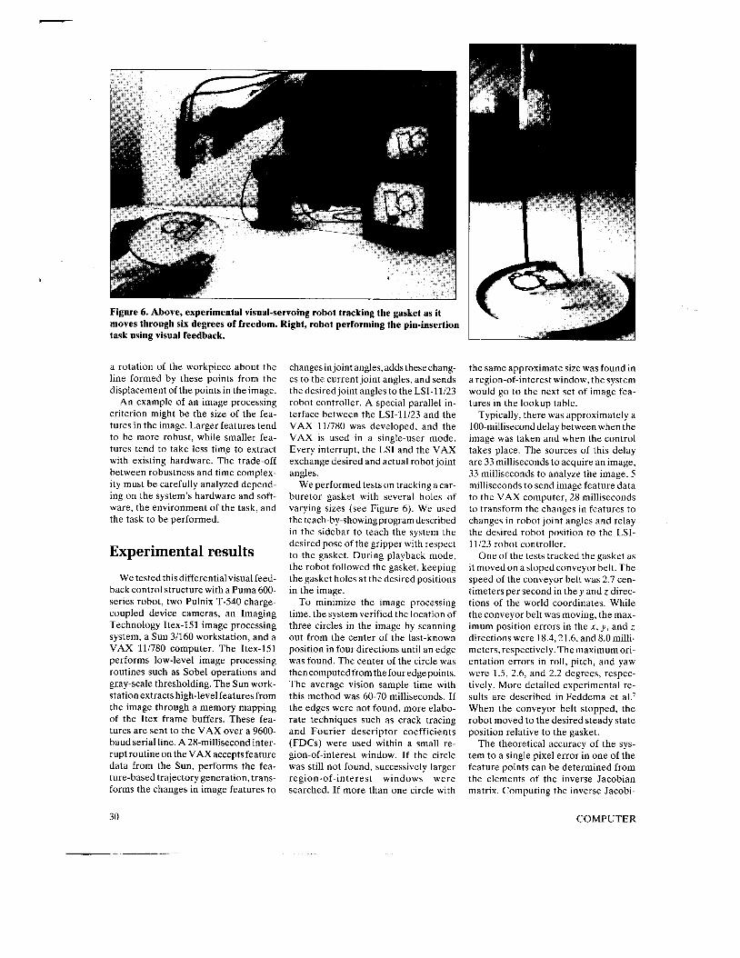
Figure 6. Above, experimental visual-servoing robot tracking the gasket as it moves through six degrees of freedom. Right, robot performing the pin-insertion task using visual feedback.

a rotation of the workpiece about the line formed by these points from the displacement of the points in the image.

An example of an image processing criterion might be the size of the features in the image. Larger features tend to be more robust, while smaller features tend to take less time to extract with existing hardware. The trade-off between robustness and time complex- ity must be carefully analyzed depend- ing on the system’s hardware and software, the environment of the task, and the task to be performed.

Experimental results

We tested this differential visual feedback control structure with a Puma 600- series robot, two Pulnix T-540 charge- coupled device cameras, an Imaging Technology Itex-151 image processing system, a Sun 3/160 workstation, and a VAX 111780 computer. The Itex-151 performs low-level image processing routines such as Sobel operations and gr,ay-scale thresholding. The Sun workstation extracts high-level features from the image through a memory mapping of the Itex frame buffers. These features are sent to the VAX over a 9600- baud serial line. A 28-millisecond interrupt routine on the VAX accepts feature data from the Sun, performs the feature-based trajectory generation, transforms the changes in image features to

changes in joint angles, adds these changes to the current joint angles, and sends the desired joint angles to the LSI-11/23 robot controller. A special parallel in- terface between the LSI-11/23 and the VAX 11/780 was developed, and the VAX is used in a single-user mode. Every interrupt, the LSI and the VAX exchange desired and actual robot joint angles.

We performed tests on tracking a carburetor gasket with several holes of varying sizes (see Figure 6). We used the teach-by-showing program described in the sidebar to teach the system the desired pose of the gripper with respect to the gasket. During playback mode, the robot followed the gasket, keeping the gasket holes at the desired positions in the image.

To minimize the image processing time, the system verified the location of three circles in the image by scanning out from the center of the last-known position in four directions until an edge was found. The center of the circle was then computed from the four edge points. The average vision sample time with this method was 60-70 milliseconds. If the edges were not found, more elabo- rate techniques such as crack tracing and Fourier descriptor coefficients (FDCs) were used within a small region-of-interest window. If the circle was still not found, successively larger region-of-interest windows were searched. If more than one circle with

the same approximate size was found in a region-of-interest window, the system would go to the next set of image features in the lookup table.

Typically, there was approximately a 100-millisecond delay between when the image was taken and when the control takes place. The sources of this delay are 33 milliseconds to acquire an image, 33 milliseconds to analyze the image, 5 milliseconds to send image feature data to the VAX computer, 28 milliseconds to transform the changes in features to changes in robot joint angles and relay the desired robot position to the LSI- 11/23 robot controller.

One of the tests tracked the gasket as it moved on a sloped conveyor belt. The speed of the conveyor belt was 2.7 cen- timeters per second in they and z directions of the world coordinates. While the conveyor belt was moving, the maximum position errors in the x , y, and z directions were 18.4,21.6, and 8.0 millimeters, respectively. The maximum orientation errors in roll, pitch, and yaw were 1.5, 2.6, and 2.2 degrees, respectively. More detailed experimental results are described in Feddema et al.’ When the conveyor belt stopped, the robot moved to the desired steady state position relative to the gasket.

The theoretical accuracy of the system to a single pixel error in one of the feature points can be determined from the elements of the inverse Jacobian matrix. Computing the inverse Jacobi-

30 COMPUTER

,

an about the desired operating point (three gasket circles forming a triangle at 200 millimeters below the camera), the theoretical maximum position errors in the .Y, y , and z directions are 3.0, 6.4, and 0.7 millimeters, respectively. The maximum orientation errors in roll, pitch, and yaw are 1.7, 0.8, and 0.2 degrees, respectively. The difference between the theoretical and experimental positioning accuracies was the result of the smoothing operation performed by the trajectory generator. In the future, as vision sampling time and servo reac- tion time decrease, accuracy will approach the theoretical limits.

-

W hile our research has shown the potential of model-based visual feedback control for a

hand-eye coordinated robotic system, real-time visual servoing for industrial use is still several years away. The dem- onstrated system has limited capabili- ties and often lacks the robustness necessary for industrial tasks. We are continuing research on both hardware and software issues.

There are two hardware bottlenecks in the current implementation. The first is the need to quickly extract robust features from an image. The second is the communication between the robot and the vision modules. A topic for software research is off-line simulation of the teaching phase. The objective would be to use CAD data instead of teach-by-showing methods to select the appropriate features for control. By using the C A D model, an entire assembly process could be planned off-line, thus eliminating the nonproductive time necessary for teaching.

Acknowledgments This work was supported in part by an

IBM research fellowship and in part by the National Science Foundation under Grant No. C D R 8803017 t o the Engineering Re- search Center for Intelligent Manufacturing Systems. Any opinions, findings, and conclu-

2. R. Tsia. “ A Versatile Camera Calibra- tion Technique for High-Accuracy 3 D Vision Metrology Using Off-the-shelf T V Cameras and Lenses.” IEEE J . Robotics und Rutonlation. Vol. RA-3, No. 4, Aug. 1987. pp. 323-344.

3. A.C. Sanderson and L.E. Weiss. “Adap- tive Visual Servo Control of Robots,” reprinted in Robor Vision, A . Pugh, ed., London: IFS Publications Ltd., pp. 107- 116. 1983.

4. D.E. Whitney, “The Mathematics of Co- ordinated Control of Prosthetic Arms and Manipulators,” Trans. ASME, J . of Dynumic Systems. Measurement, arid Con- trol. Vol. 122, Dec. 1972, pp. 303-309.

5. S. Arimoto and F. Miyazaki, “Stability and Robustness of PID Feedback Con- trol for Robot Manipulators of Sensory Capability,” Proc. Int’l Symp. Robotics Research. M I T Press, Cambridge. Mass., 1983, pp. 783-799.

6. L.E. Weiss, A.C. Sanderson. and C.P. Neuman, “Dynamic Sensor-Based Con- trol of Robots with Visual Feedback,” IEEE J . of Robotics and Automation, Vol. RA-3,No. 5, Oct. 1987. pp. 404-417.

7. J .T . Feddema, C.S.G. Lee, and O . R . Mitchell, “Weighted Selection of Image Features for Resolved Rate Visual Feed- back Control,” IEEE Trans. Roboticsand Automation, Vol. 7. No. 1, Feb. 1991, pp. 31-47.

8. K.S. Fu, R.C. Gonzalez, and C.S.G. Lee. Robotics: Control. Sensing, Vision. and Intelligence. McGraw-Hill, 1987.

9. C. Samson, M. Le Borgne, and B. Espiau, Robot Control: The Task Functiori A p - proacli, Oxford Univ., New York, 1991, pp. 2 18-235.

I O . J.T. Feddema and O.R. Mitchell. “Vision Guided Servoing with Feature-BasedTra- jectory Generation.” IEEE Trans. Ro- botics and Automation. Vol. 5. No. 5, 1989. pp. 69 1-670.

Feddema received the BSEE degree f rom Iowa State University in 1984 and the M S E E and P h D degrees from Purdue University in 1986 and 1989, respectively. H e is a member o f t h e I E E E .

C.S. George Lee is a professor in the School of Electrical Engineering, Purdue Universi- ty, West Lafayette. Indiana. His research interests include computational robotics, intel. ligent multirobot assembly systems, and fuzzy neural networks.

Lee received his BS and MS in electrical engineering from Washington State Univer- sity in 1973 and 1974. respectively, and his P h D from Purdue University in 1978. H e is vice president of technical affairs for the I E E E Robotics and Automation Society, technical editor of the IEEE Trurisactions on Robotics and Auromation, associate editor of the Itz- ternutional Journal o f Robotics and Automa- tion, coauthor of Robotics: Coritrol, Sensing, Vision. and Intelligence. and coeditor of Tu- torial on Robotics, Second Edition. H e is a senior member of the IEEE.

0. Robert Mitchell is professor and chair of electrical engineering at the University of Texas at Arlington. H e previously taught at Purdue University where he also served as assistant dean of engineering for industrial relations and research, and associate director of the National Science Foundation’s Engi- neering Research Center for Intelligent Man- ufacturing Systems. His research interests a re in automated inspection. reverse engineering, intelligent material handling, robotic surface finishing. shape and texture analysis, and precision measurements in images.

Mitchell received the BSEE from Lamar University in 1967 and the S M E E and P h D degrees from MIT in 1968 and 1972. respec- . .

sions or recommendations expressed in this article are those of the authors and d o not necessarily reflect thc views Of the funding agencies.

John T. ~ ~ d d ~ ~ ~ is a senior of the technical staff at rics in Albuquerque, New He has worked in the Intelligent Systems Sensor and Controls Deoartment on the control of flex-

tively. H e served as vice chair of the Midconi 90 Technical Program Committee and secre- t a r y h e a s u r e r of the Central Indiana chapter of the I E E E Computer Society. H e is asenior member

National

ible robotic structures and multisensor integration of chemical and radiological sensors for nuclear waste characterization. Additional research interests include robotics, comput- e r vision. scnsor-based control, and comput-

References Readers may contact John Feddema. at

Sandia National Laboratorics, Department 161 1. P O Box 5800, Albuquerque. NM 87185:

I . R.P. Paul, Robot Manipulators: Mathe- mcrtics. Programming, and Control, M I T Press. Cambridge, Mass., 1981. er-integrated manufacturing. e-mail, feddema~~cs .sandia .gov .

August 1 Y Y 2 31

Documents

Model-based visual feedback control for a hand-eye coordinated robotic system