Model Building Training - Yale Universityzoo.cs.yale.edu/classes/cs445/slides/Yale1.pdf · of the outcome between the training and test sets – A SR split is more appropriate for

1

Model Building:General Strategies, Data Pre-processing,

and Partial Least Squares

Max Kuhn and Kjell JohnsonNonclinical Statistics, Pfizer

1Monday, March 24, 2008

2

Objective

To construct a model of predictors that can be used to predict a response

Data

Model

Prediction


http://home.pfizer.com/








3

Model Building Steps

• Common steps during model building are:– estimating model parameters (i.e. training models)– determining the values of tuning parameters that

cannot be directly calculated from the data– calculating the performance of the final model that will

generalize to new data• The modeler has a finite amount of data, which

they must "spend" to accomplish these steps– How do we “spend” the data to find an optimal model?


4

“Spending” Data

• We typically “spend” data on training and test data sets– Training Set: these data are used to estimate model parameters

and to pick the values of the complexity parameter(s) for the model.

– Test Set (aka validation set): these data can be used to get an independent assessment of model efficacy. They should not be used during model training.

• The more data we spend, the better estimates we’ll get (provided the data is accurate). Given a fixed amount of data,– too much spent in training won’t allow us to get a good

assessment of predictive performance. We may find a model that fits the training data very well, but is not generalizable (overfitting)

– too much spent in testing won’t allow us to get a good assessment of model parameters


5

Methods for Creating a Test Set

• How should we split the data into a training and test set?

• Often, there will be a scientific rational for the split and in other cases, the splits can be made empirically.

• Several empirical splitting options:– completely random– stratified random– maximum dissimilarity in predictor space


6

Creating a Test Set: Completely Random Splits

• A completely random (CR) split randomly partitions the data into a training and test set

• For large data sets, a CR split has very low bias towards any characteristic (predictor or response)

• For classification problems, a CR split is appropriate for data that is balanced in the response

• However, a CR split is not appropriate for unbalanced data– A CR split may select too few observations (and perhaps none) of

the less frequent class into one of the splits.


7

Creating a Test Set: Stratified Random Splits

• A stratified random split makes a random split within stratification groups– in classification, the classes are used as strata– in regression, groups based on the quantiles of the

response are used as strata

• Stratification attempts to preserve the distribution of the outcome between the training and test sets– A SR split is more appropriate for unbalanced data


8

Over-Fitting

• Over-fitting occurs when a model has extremely good prediction for the training data but predicts poorly when– the data are slightly perturbed– new data (i.e. test data) are used

• Complex regression and classification models assume that there are patterns in the data.– Without some control many models can find very intricate

relationships between the predictor and the response– These patterns may not be valid for the entire population.


9

Over-Fitting Example

• The plots below show classification boundaries for two models built on the same data– one of them is over-fit

Pre

dict

or B

Pre

dict

or B

Predictor A Predictor A


10

Over-Fitting in Regression

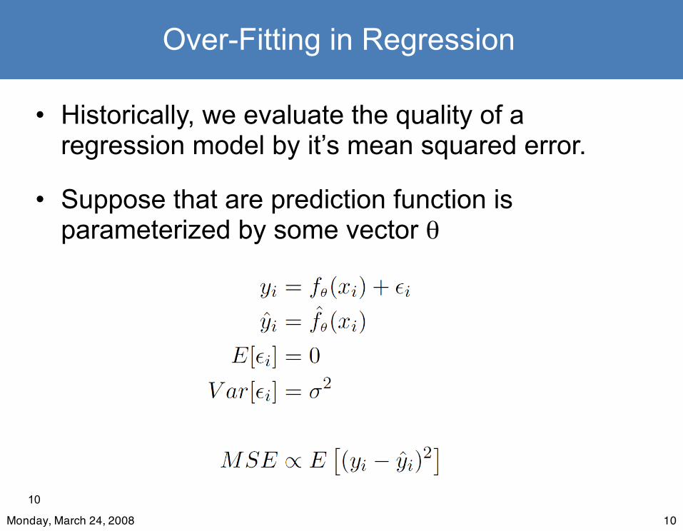
• Historically, we evaluate the quality of a regression model by it’s mean squared error.

• Suppose that are prediction function is parameterized by some vector θ


11


• MSE can be decomposed into three terms:– irreducible noise– squared bias of the estimator from it’s expected value– the variance of the estimator

• The bias and variance are inversely related– as one increases, the other decreases– different rates of change


12


• When the model under-fits, the bias is generally high and the variance is low

• Over-fitting is typically characterized by high variance, low bias estimators

• In many cases, small increases in bias result in large decreases in variance


13


• Generally, controlling the MSE yields a good trade-off between over- and under-fitting– a similar statement can be made about classification

models, although the metrics are different (i.e. not MSE)

• How can we accurately estimate the MSE from the training data?– the naïve MSE from the training data can be a very

poor estimate

• Resampling can help estimate these metrics


14

How Do We Estimate Over-Fitting?

• Some models have specific “knobs” to control over-fitting– neighborhood size in nearest neighbor models is an

example– the number if splits in a tree model

• Often, poor choices for these parameters can result in over-fitting

• Resampling the training compounds allows us to know when we are making poor choices for the values of these parameters


15

How Do We Estimate Over-Fitting?

• Resampling only affects the training data– the test set is not used in this procedure

• Resampling methods try to “embed variation” in the data to approximate the model’s performance on future compounds

• Common resampling methods:– K-fold cross validation– Leave group out cross validation– Bootstrapping


16

K-fold Cross Validation

• Here, we randomly split the data into K blocks of roughly equal size

• We leave out the first block of data and fit a model.

• This model is used to predict the held-out block• We continue this process until we’ve predicted all

K hold-out blocks• The final performance is based on the hold-out

predictions


17

K-fold Cross Validation

• The schematic below shows the process for K = 3 groups.– K is usually taken to be 5 or 10– leave one out cross-validation has each sample as a

block


18

Leave Group Out Cross Validation

• A random proportion of data (say 80%) are used to train a model

• The remainder is used to predict performance

• This process is repeated many times and the average performance is used




19

Bootstrapping

• Bootstrapping takes a random sample with replacement– the random sample is the same size as the original

data set– compounds may be selected more than once– each compound has a 63.2% change of showing up at

least once• Some samples won’t be selected

– these samples will be used to predict performance• The process is repeated multiple times (say 30)


20

The Bootstrap

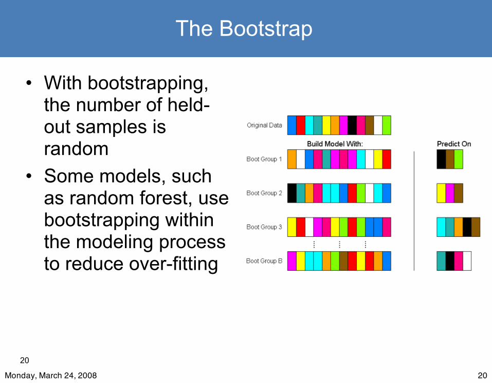
• With bootstrapping, the number of held-out samples is random

• Some models, such as random forest, use bootstrapping within the modeling process to reduce over-fitting




21

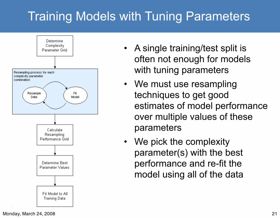
Training Models with Tuning Parameters

• A single training/test split is often not enough for models with tuning parameters

• We must use resampling techniques to get good estimates of model performance over multiple values of these parameters

• We pick the complexity parameter(s) with the best performance and re-fit the model using all of the data













22

Simulated Data Example

• Let’s fit a nearest neighbors model to the simulated classification data.

• The optimal number of neighbors must be chosen• If we use leave group out cross-validation and set

aside 20%, we will fit models to a random 200 samples and predict 50 samples– 30 iterations were used

• We’ll train over 11 odd values for the number of neighbors– we also have a 250 point test set


23

Toy Data Example

• The plot on the right shows the classification accuracy for each value of the tuning parameter– The grey points are the 30

resampled estimates– The black line shows the average

accuracy – The blue line is the 250 sample

test set

• It looks like 7 or more neighbors is optimal with an estimated accuracy of 86%













24

Toy Data Example

• What if we didn’t resample and used the whole data set?

• The plot on the right shows the accuracy across the tuning parameters

• This would pick a model that over-fits and has optimistic performance













25

Data Pre-Processing





26

Why Pre-Process?

• In order to get effective and stable results, many models require certain assumptions about the data– this is model dependent

• We will list each model’s pre-processing requirements at the end

• In general, pre-processing rarely hurts model performance, but could make model interpretation more difficult


27

Common Pre-Processing Steps

• For most models, we apply three pre-processing procedures:– Removal of predictors with variance close to zero

– Elimination of highly correlated predictors

– Centering and scaling of each predictor


28

Zero Variance Predictors

• Most models require that each predictor have at least two unique values

• Why?– A predictor with only one unique value has a variance

of zero and contains no information about the response.

• It is generally a good idea to remove them.


29

“Near Zero Variance” Predictors

• Additionally, if the distributions of the predictors are very sparse,– this can have a drastic effect on the stability of the

model solution– zero variance descriptors could be induced during

resampling

• But what does a “near zero variance” predictor look like?


30

“Near Zero Variance” Predictor

• There are two conditions for an “NZV” predictor– a low number of possible values, and– a high imbalance in the frequency of the values

• For example, a low number of possible values could occur by using fingerprints as predictors– only two possible values can occur (0 or 1)

• But what if there are 999 zero values in the data and a single value of 1?– this is a highly unbalanced case and could be trouble


31

NZV Example

• In computational chemistry we created predictors based on structural characteristics of compounds.

• As an example, the descriptor “nR11” is the number of 11-member rings

• The table to the right is the distribution of nR11 from a training set– the distinct value percentage is

5/535 = 0.0093– the frequency ratio is 501/23 = 21.8

# 11-Member RingsValue Frequency

0 5011 42 233 54 2


32

Detecting NZVs

• Two criteria for detecting NZVs are the– Discrete value percentage

• Defined as the number of unique values divided by the number of observations

• Rule-of-thumb: discrete value percentage < 20% could indicate a problem

– Frequency ratio• Defined as the frequency of the most common value divided by the

frequency of the second most common value• Rule-of-thumb: > 19 could indicate a problem

• If both criteria are violated, then eliminate the predictor


33

Highly Correlated Predictors

• Some models can be negatively affected by highly correlated predictors– certain calculations (e.g. matrix inversion) can

become severely unstable

• How can we detect these predictors?– Variance inflation factor (VIF) in linear regression or, alternatively1. Compute the correlation matrix of the predictors2. Predictors with (absolute) pair-wise correlations

above a threshold can be flagged for removal3. Rule-of-thumb threshold: 0.85


34

Highly Correlated Predictors and Resampling

• Recall that resampling slightly perturbs the training data set to increase variation

• If a model is adversely affected by high correlations between predictors, the resampling performance estimates can be poor in comparison to the test set– In this case, resampling does a better job at predicting

how the model works on future samples


35

Centering and Scaling

• Standardizing the predictors can greatly improve the stability of model calculations.

• More importantly, there are several models (e.g. partial least squares) that implicitly assume that all of the predictors are on the same scale

• Apart from the loss of the original units, there is no real downside of centering and scaling


36

An Example





37

in-silico Chemistry Modeling

• Chemists like to use the molecular structure of a compound to predict some outcome, such as– activity against some biological target– toxicity– solubility and other outcomes

• The relate the structure to the outcome, molecular descriptors are computed from the “formula” of a compound

O[C@H](CCn1c(c2ccc(F)cc2)c(c2ccccc2)c(C(=O)Nc2ccccc2)c1C(C)C)C[C@@H](O)CC(= O)O

=


38

Mutagenicity Data

• Kazius (2005) investigated using chemical structure to predict mutagenicity (the increase of mutations due to the damage to genetic material).

• An Ames test was used to evaluate the mutagenicity potential of various chemicals.

• There were 4,337 compounds included in the data set with a mutagenicity rate of 55.3%.


39

Mutagenicity Data

• Using these compounds, the DragonX software was used to generate a baseline set of 1,579 predictors, including constitutional, topological and connectivity descriptors, among others.

• These variables consist of basic numeric variables (such as molecular weight) and counts variables (e.g. number of halogen atoms).

• The data were split into a training (n = 3,252) and a test set (n = 1,083)


40

Zero-Variance Predictors

• The simple training/test split caused three predictors to become zero-variance in the training set.

• Filtering on near-zero variance descriptors would eliminate 272 predictors from the training set.

•


41

Highly Correlated Predictors

• For this type of data, there are usually a lot of highly correlated predictors.– the plot on the top right has

all pair-wise correlations

• Removing predictors with correlations above 0.90 removes 926 predictors– this will help when we look

at predictor importance




42

Tuning a Support Vector Machine

• With SVMs, there are usually 2-3 tuning parameters:– the cost function– kernel parameters

• For radial basis functions, the kernel parameter is the sigma in

• We’ll use a trick from Caputo et al (2002) to analytically estimate a reasonable value of the kernel parameter


43

Tuning a Support Vector Machine

• We tried 5 values of the tuning parameter:– 0.1, 1, 10, 100 and 1,000– sigma was estimated to be 0.000448

• For each of the 5 combinations, we have 25 bootstrap estimates of the accuracy and Kappa statistics


44

Tuning Results

• Each point on the graph is an average of the 25 bootstrap estimates of performance

• We could go with cost value of 10– This results in 1,618

support vectors (49% of the training set)

log10 Cost

Accura

cy

0.72

0.74

0.76

0.78

0.80

0.82

!1 0 1 2 3

!

!

!

!

!

log10 Cost

Kappa

0.40

0.45

0.50

0.55

0.60

!1 0 1 2 3

!

!

!

!

!













45

Tuning Results

• Using the bootstrap estimates, we can also get a sense of the uncertainty in performance

• Resampling and the test set give comparable performance for this data set/model

Training Test Accuracy 81.8 84.2 (81.9, 86.3)

Kappa 0.63 0.68

Density

010

20

30

40

0.80 0.82 0.84

Accuracy

05

10

15

20

0.60 0.65 0.70

Kappa













46

Partial Least Squares Regression





47

When Does Linear Regression Fail?

• When a plane does not capture the structure in the data• When the variance/covariance matrix is overdetermined

– Recall, the plane that minimizes SSE is:

– To find the best plane, we must compute the inverse of the variance/covariance matrix

– The variance/covariance matrix is not always invertible. Two common conditions that cause it to be uninvertible are:

• Two or more of the predictors are correlated (multicollinearity)• There are more predictors than observations


48

Solutions for Overdetermined Covariance Matrices

• Variable reduction– Try to accomplish this through the pre-processing

steps• Partial least squares (PLS)• Other methods

– Apply a generalized inverse– Ridge regression: Adjusts the variance/covariance

matrix so that we can find a unique inverse.– Principal component regression (PCR)

• not recommended—but it’s a good way to understand PLS


49

Understanding Partial Least Squares:Principal Components Analysis

• PCA seeks to find linear combinations of the original variables that summarize the maximum amount of variability in the original data– These linear combinations are often called principal

components or scores.

– A principal direction is a vector that points in the direction of maximum variance.


50

Principal Components Analysis

• PCA is inherently an optimization problem, which is subject to two constraints1.The principal directions have unit length2.Either

a.Successively derived scores are uncorrelated to previously derived scores, OR

b.Successively derived directions are required to be orthogonal to previously derived directions

• In the mathematical formulation, either constraint implies the other constraint


51

-4

-3

-2

-1

0

1

2

3

4

5

-6 -5 -4 -3 -2 -1 0 1 2 3 4 5

Predictor 1

Pred

icto

r 2Principal Components Analysis


51

-4

-3

-2

-1

0

1

2

3

4

5

-6 -5 -4 -3 -2 -1 0 1 2 3 4 5

Predictor 1

Pred

icto

r 2

Direction 1



51

-4

-3

-2

-1

0

1

2

3

4

5

-6 -5 -4 -3 -2 -1 0 1 2 3 4 5

Predictor 1

Pred

icto

r 2

Direction 1



51

-4

-3

-2

-1

0

1

2

3

4

5

-6 -5 -4 -3 -2 -1 0 1 2 3 4 5

Predictor 1

Pred

icto

r 2

Direction 1

Score



PCA in Action

52


53

Mathematically Speaking…

• The optimization problem defined by PCA can be solved through the following formulation:

subject to constraints 2a. or b.• Facts…

– the ith principal direction, ai, is the eigenvector corresponding to the ith largest eigenvalue of XTX.

– the ith largest eigenvalue is the amount of variability summarized by the ith principal component.

– are the ith scores


54

PCA Benefits and Drawbacks

• Benefits– Dimension reduction

• We can often summarize a large percentage of original variability with only a few directions

– Uncorrelated scores• The new scores are not linearly related to each other

• Drawbacks– PCA “chases” variability

• PCA directions will be drawn to predictors with the most variability• Outliers may have significant influence on the directions and

resulting scores.


55

Principal Component Regression

Procedure:

1. Reduce dimension of predictors using PCA 2. Regress scores on response

Notice: The procedure is sequential


56

Dimension reduction is independent of the objective

PredictorVariables

PC Scores

ResponseVariable

PCA

MLR

Principal Component Regression











57

-5.00

-2.25

0.50

3.25

6.00

-5.00 -3.75 -2.50 -1.25 0 1.25 2.50 3.75 5.00

Scatter of Predictors

Pred

icto

r 2

Predictor 1

First Principal Direction


58

-5.00

-3.75

-2.50

-1.25

0

1.25

2.50

3.75

5.00

-6 -2 2 6 10

Scatter of First PCA Scores with Response

Res

pons

e

First PCA Scores

Relationship of First Direction with Response


59

PLS History

• H. Wold (1966, 1975)• S. Wold and H. Martens (1983)• Stone and Brooks (1990)• Frank and Friedman (1991, 1993)• Hinkle and Rayens (1994)


60

Latent Variable Model

Predictor2

Predictors Responses

Response1

Predictor1

Predictor3

Predictor4

Predictor5

Latent Variables

γ1

γ2

π

Predictor6

Response2

Response3

Note: PLS can handle multiple response variables


61

Comparison with Regression

Predictor1

Predictor2

Predictor3

Predictor4

Predictor5

Response1




















62

PLS Optimization(many predictors, one response)

• PLS seeks to find linear combinations of the independent variables that summarize the maximum amount of co-variability with the response.– These linear combinations are often called PLS

components or PLS scores.

– A PLS direction is a vector that points in the direction of maximum co-variance.


63

PLS Optimization(many predictors, one response)

• PLS is inherently an optimization problem, which is subject to two constraints1.The PLS directions have unit length2.Either

a.Successively derived scores are uncorrelated to previously derived scores, OR

b.Successively derived directions are orthogonal to previously derived directions

• Unlike PCA, either constraint does NOT imply the other constraint

• Constraint 2.a. is most commonly implemented


64

Mathematically Speaking…

• The optimization problem defined by PLS can be solved through the following formulation:

subject to constraints 2a. or b.• Facts…

– the ith PLS direction, ai, is the eigenvector corresponding to the ith largest eigenvalue of ZTZ, where Z = XTy.

– the ith largest eigenvalue is the amount of co-variability summarized by the ith PLS component.

– are the ith scores


65

PLS is Simultaneous Dimension Reduction and Regression













66

PLS is Simultaneous Dimension Reduction and Regression

max Var(scores) Corr2(response,scores)

Dimension Reduction(PCA)

Regression


67

PLS Benefits and Drawbacks

• Benefit– Simultaneous dimension reduction and regression

• Drawbacks– Similar to PCA, PLS “chases” co-variability

• PLS directions will be drawn to independent variables with the most variability (although this will be tempered by the need to also be related to the response)

• Outliers may have significant influence on the directions, resulting scores, and relationship with the response. Specifically, outliers can

– make it appear that there is no relationship between the predictors and response when there truly is a relationship, or

– make it appear that there is a relationship between the predictors and response when there truly is no relationship


68

Simultaneous dimension reduction and regression

PredictorVariables

ResponseVariable

PLS

Partial Least Squares


69

-5.000

-3.167

-1.333

0.500

2.333

4.167

6.000

-5.8333 -4.0278 -2.2222 -0.4167 1.3889 3.1944 5.0000

Scatter of Predictors

Pred

icto

r 2

Predictor 1

First PLS Direction


70

-5.00

-3.75

-2.50

-1.25

0

1.25

2.50

3.75

5.00

-5.00 -3.75 -2.50 -1.25 0 1.25 2.50 3.75 5.00

Scatter of First PLS Scores with Response

Res

pons

e

First PLS Scores

Relationship of First Direction with Response


71

PLS in Practice

• PLS seeks to find latent variables (LVs) that summarize variability and are highly predictive of the response.

• How do we determine the number of LVs to compute?– Evaluate RMSPE (or Q2)

• The optimal number of components is the number of components that minimizes RMSPE


72

Boston Housing Data

• This is a classic benchmark data set for regression. It includes housing data for 506 census tracts of Boston from the 1970 census.

• crim: per capita crime rate• Indus: proportion of non-retail

business acres per town • chas: Charles River dummy

variable (= 1 if tract bounds river; 0 otherwise)

• nox: nitric oxides concentration • rm: average number of rooms

per dwelling • Age: proportion of owner-

occupied units built prior to 1940

• dis: weighted distances to five Boston employment centers

• rad: index of accessibility to radial highways

• tax: full-value property-tax rate • ptratio: pupil-teacher ratio by

town • b: proportion of minorities• Medv: median value homes

(outcome)


73

PLS for the Boston housing data:Training the PLS Model

• Since PLS can handle highly correlated variables, we fit the model using all 12 predictors

• The model was trained with up to 6 components

• RMSE drops noticeably from 1 to 2 components and some for 2 to 3 components.– Models with 3 or more

components might be sufficient for these data




74

Training the PLS Model

• Roughly the same profile is seen when the models are judged on R2




Documents

Model Building Training - Yale Universityzoo.cs.yale.edu/classes/cs445/slides/Yale1.pdf · of the outcome between the training and test sets – A SR split is more appropriate for