Model Checking Using SMT and Theory of Lists

Aleksandar Milicevic1 and Hillel Kugler2

1 Massachusetts Institute of Technology (MIT), Cambridge, MA, USAaleks@csail.mit.edu

2 Microsoft Research, Cambridge, UKhkugler@microsoft.com

Abstract. A main idea underlying bounded model checking is to limitthe length of the potential counter-examples, and then prove proper-ties for the bounded version of the problem. In software model checking,that means that only program traces up to a given length are consid-ered. Additionally, the program’s input space must be made finite bydefining bounds for all input parameters. To ensure the finiteness of theprogram traces, these techniques typically require that all loops are ex-plicitly unrolled some constant number of times. Here, we show how toavoid explicit loop unrolling by using the SMT Theory of Lists to modelfeasible, potentially unbounded program traces. We argue that this ap-proach is easier to use, and, more importantly, increases the confidence inverification results over the typical bounded approach. To demonstratethe feasibility of this idea, we implemented a fully automated prototypesoftware model checker and verified several example algorithms. We alsoapplied our technique to a non software model-checking problem frombiology – we used it to analyze and synthesize correct executions fromscenario-based requirements in the form of Live Sequence Charts.

1 Introduction

We present a finite-state model-checking technique, based on satisfiability solv-ing, that does not require the user to explicitly bound the length of the searchtraces. We use the SMT Theory of Lists [7] to model potentially infinite searchtraces. A benefit of this approach is that it does not require providing the numberof loop unrollings. Similarly, when trying to solve a planning problem, we do nothave to specify the maximum number of steps needed to solve the problem. Thisway, we can achieve most of the benefits of the unbounded case. Unfortunately,in some cases our approach cannot prove that no counter-example exists (e.g.,in the presence of infinite loops in the program), so it is not fully unbounded.

We use a list to model an unbounded search path. Every list element rep-resents a single state traversed during the search. In order to find a path to anerror state, we impose the following constraints on that list: (1) the first elementis a valid initial state, (2) every two consecutive elements represent a valid statetransition; and (3) the last element corresponds to one of the states we wantto reach (error states). Having formulated the problem in this way, we can runan SMT solver, namely Z3 [23], to search for such a list, without constrainingits length. If Z3 terminates and reports that the problem is unsatisfiable, we

have proved that the error states are unreachable; otherwise, we have found acounter-example.

This idea is readily applicable to software model checking. In the presence ofloops, program traces become infinite. A common resort is to explicitly performloop unrolling, as it is the case with CBMC [10], Forge [16] and [5]. The limitationof this approach is that the number of unrollings must be specified beforehandby the user. Typically, the number of unrollings and the bounds for the inputspace are specified independently of each other, even though they are almostnever independent in practice. For example, in order to verify the “selectionsort” algorithm for arrays of length up to N , at least N − 1 loop unrollingsare needed. If the user provides a number less than N − 1, a tool for boundedverification will typically report that no counter-example can be found withinthe given bounds, which may trick the user into believing that the algorithmis proven to be correct for all arrays of length up to N . With our approach,to verify the “selection sort” algorithm, the user only specifies the bound forN . Bounds for array elements are not needed in this case, so we can prove thealgorithm correct for all integer arrays up to the given length N .

The main contributions of this paper are:

– A novel approach to model checking using SMT and the theory of lists: weexplain how lists can be used to model unbounded traces;

– Application of this idea to software model checking: we present an optimizedencoding of a program, and show that loops need not be explicitly unrolled;

– Execution of Live Sequence Charts case study: we analyzed scenario-basedmodels of biological systems [19], written in the language of Live SequenceCharts (LSC) [15]. We show that declarative scenario-based specifications,written in LSC, can be translated into the logic of SMT, and an off-the-shelfsolver can be used to automatically execute them.

2 Background

In order to check whether a safety property holds within some number of statesk, one can define k sets of variables, one set for each state, s1, s2, · · · , sk, andthen, as with any model-checking problem, assert that the following hold:

1. Initial State constraint: Θ(s1);2. Transition constraint: ρ(s1, s2) ∧ ρ(s2, s3) ∧ · · · ∧ ρ(sk−1, sk); and3. Safety Property constraint: P(s1) ∧ P(s2) ∧ · · · ∧ P(sk−1) ∧ ¬P(sk).

Θ encodes constraints that must hold in the initial state; ρ(si−1, si) is atransition function which returns true if and only if the system is allowed to gofrom state si−1 to state si; finally, P(si) is the safety property that we wantto prove. In order to find a counter-example, we assert that the safety propertydoesn’t hold in the last state while holding in all previous states. Additionally, thetransition function must hold for every two consecutive states. The conjunctionof these three formulas is passed to an off-the-shelf solver, which either returnsa model encoding a counter-example, or proves that the formula is unsatisfiable

(meaning that the safety property is verified for the given k). This approach iscommonly referred to as bounded model checking using satisfiability solving.

We focus on how to use the theory of lists to avoid having k copies of thestate variables. The theory of lists is currently supported by many state-of-the-art SMT solvers. A description of how other theories can be used to encodeprograms and why that can be advantageous is presented in [5].

SMT lists are defined recursively: List<E> = nil | cons (head: E, tail:

List). For a given list, only two fields, head and tail are immediately acces-sible. In addition, predicates is cons and is nil are readily available to checkwhether a given list variable is cons or nil. As a consequence, it is not possibleto directly access the list element at a given position, or immediately get thelength of the list, which is inconvenient when asserting properties about lists.

3 Approach

Our approach is based on the idea of bounded model checking using satisfiabilitysolving, except that instead of explicitly enumerating all state variables (s1, s2,· · · , sk), and thus bounding the length of a potential counter-example, we useonly a single variable of type List of States. Every list element is of type State,which is a tuple of all variables needed to represent the problem state. We stillassert the same three constraints, (1) initial state, (2) transition; and (3) safetyconstraint, but now in terms of a single list variable.

Expressing the initial state constraint is easy, since the first element of thelist is immediately accessible. To express the other two constraints, we use anuninterpreted function accompanied with an axiom. More precisely, in orderto enforce the transition constraint between every two consecutive elements ofthe list, we first define an uninterpreted function, named check tr, that takes alist and returns a boolean value. Next we add an axiom (transition axiom) toassert that check tr returns true when applied to a list if and only if every twoconsecutive states of that list represent a valid state transition.

A recursive definition of the transition axiom is given in Figure 1. The onlycase of importance is when the list argument, namely lst, is not nil and hasa non-nil next element (tail). This is because we only care to assert the tran-sition property between two consecutive elements. We do that by inlining theactual model-checking transition constraint between the current and the nextlist element. In addition, we have to make sure that all subsequent consecutiveelements represent valid state transitions, so we recursively assert that the samecheck tr function returns true for the tail of the given list argument.

In order to enforce the safety property on all list elements but the last one, wecould similarly define another uninterpreted function and an additional axiom.However, since we already have an axiom that “traverses” the whole list, wedecided to include the safety property check in the existing transition axiom.This can simply be done by checking whether the next list element (tail(lst))corresponds to an error state (by inlining the error condition, i.e. ¬P(si)). If thenext element is in fact an error state, we have found a counter-example, so we

force the list to end right there (i.e. its next element must be nil). Otherwise,we must keep searching, so the next element in the list must be cons.

Finally, it is important to stress the purpose of the instantiation pattern (PAT:{check tr (lst)}) in the FORALL clause. This axiom states something about alllists. However, it would be impossible for the SMT solver to try to prove that thestatement indeed holds for all possible lists. Instead, the common approach is toprovide an instantiation pattern to basically say in which cases the axiom shouldbe instantiated and therefore enforced by the solver. In our case, we simply saythat every time we apply check tr function to a list, the axiom must be enforced,so that the evaluation of check tr indeed indicates whether the list satisfies bothtransition and safety property constraints.

DEF check tr: StateList → bool

ASSERT FORALL lst: StateList

IF (is cons(lst) ∧ is cons(tail(lst))) THEN

transition condition(head(lst), head(tail(lst))) ∧check tr(tail(lst)) ∧IF (error condition(tail(lst)))

THEN is nil(tail(tail(lst)))

ELSE is cons(tail(tail(lst)))

:PAT {check tr(lst)}

Fig. 1: Axiom for the check tr function

DEF states: StateList

ASSERT

is cons(states) ∧initial condition(head(states)) ∧check tr(states)

CHECK

Fig. 2: SMT logic context

The rest of the SMT logic context is given in Figure 2. It provides a generictemplate for model-checking problems. For a specific problem, the user onlyneeds to define: (1) the State tuple (basically enumerate all state variables), (2)initial condition, (3) transition condition; and (4) error condition.

4 Applicability to Software Model Checking

4.1 The Idea

We observe a program as a traditional Control Flow Graph (CFG) [3]. The stateof the execution of a program consists of the current basic block (at a givenmoment, the execution is exactly in a single basic block) and the evaluationsof relevant program variables. The edges between the basic blocks are calledtransitions. An edge is guarded by a logic condition that specifies when theprogram execution is allowed to go from one basic block to another. The goal ofmodel checking is to find a feasible execution trace (a path in the CFG) fromthe start node to one of the error nodes.

Programs with loops have cyclic control flow graphs, which means that someof their traces are infinite. Using unbounded lists seems like a very natural way tomodel program traces. Instead of truncating loops up front, we let the satisfiabil-ity solver simulate them, by effectively executing loops until the loop conditionbecomes false. Even though some traces may be infinite, the number of basic

blocks is always finite, meaning that the transition condition (i.e. the logic ex-pression that defines all valid transitions from a given state) is also finite andcan be expressed in a closed form.

4.2 Formal Definitions

Program Graph (PG) We formally introduce Program Graphs, which are avariation of Control Flow Graphs.

A PG is defined over a set of typed variables V ar. We will use Eval(V ar)to denote the set of possible evaluations of variables, Expr(V ar) to denote theset of all expressions over V ar (e.g., constants, integer arithmetic, “select” and“store” operations over integer arrays, and boolean expressions), and Cond(V ar)to denote the set of all boolean expressions over V ar (Cond(V ar) ⊂ Expr(V ar)).A PG is then defined as a tuple:

PG = (L,Act,Eff,→, l0,E)

L is a set of program locations (corresponding to basic blocks), l0 is the startlocation (l0 ∈ L) and E is a set of error locations (E ⊂ L). Act is a set of actions(program statements) and function Eff : Act×Eval(V ar) 7→ Eval(V ar) defines theeffects of actions on variable evaluations. Finally, →: L× Cond(V ar)×Act× L isthe conditional transition relation with side effects (i.e., actions assigned to it).This definition is very similar to the one presented in [6].

The semantics of the → relation is defined by the following rule

η |= g η′ = Eff(α, η)

〈l, η〉 g:α→ 〈l′, η′〉

where the notation lg:α→ l′ is a shorthand for (l, g, α, l′) ∈→.

4.3 Example

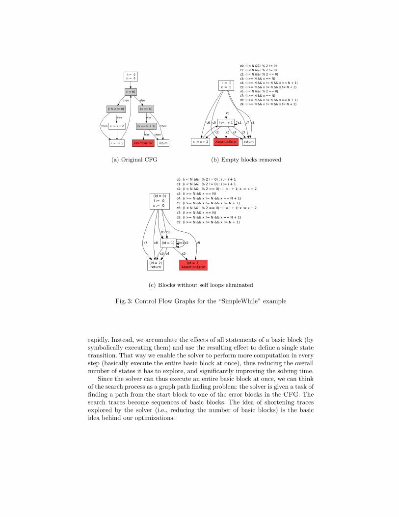
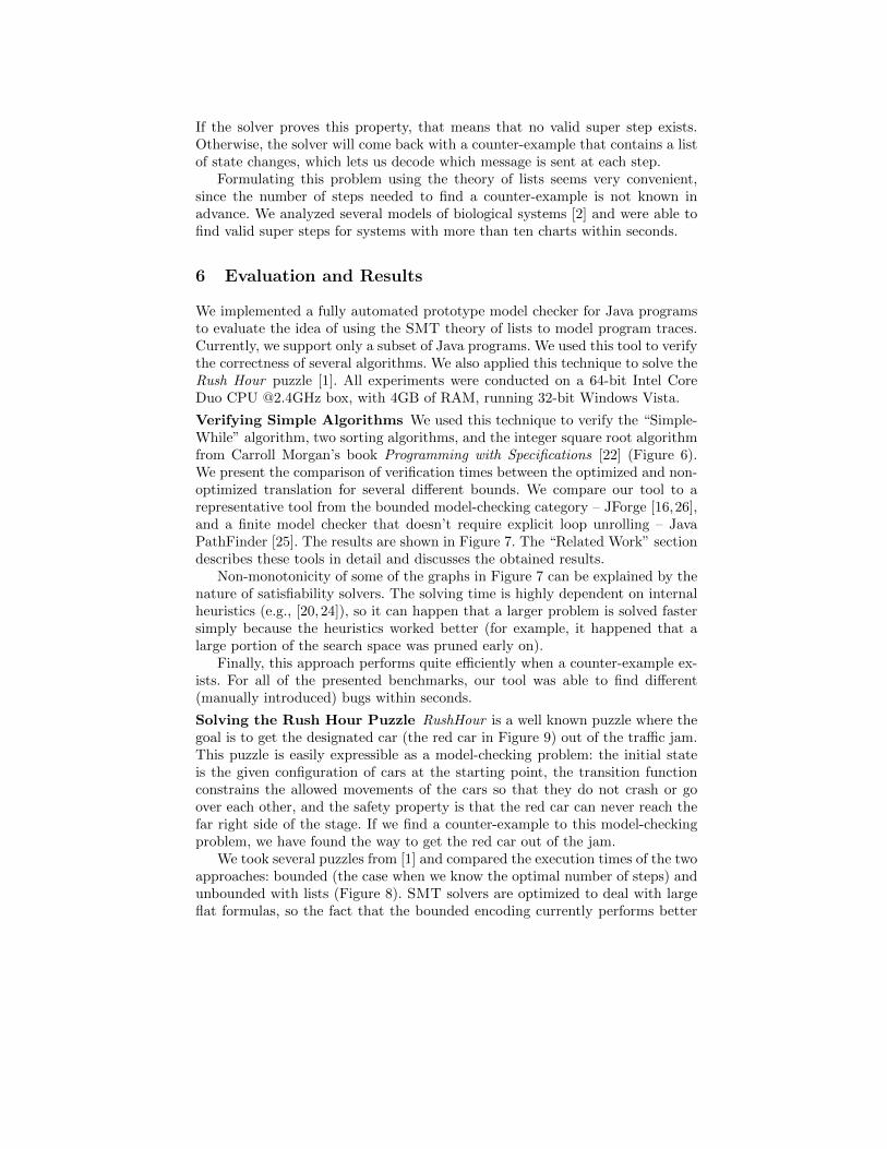
We introduce a simple example that will be used throughout this section to ex-plain optimizations and the actual translation to SMT logic. The code is shownin Figure 6, the algorithm is named simpleWhile, the corresponding CFG isshown in Figure 3(a). Blocks with grey background are simply branch condi-tions, and they do not modify the program state. The red block represents theerror state. All steps presented here are fully automated.

4.4 Optimizing Transformations from CFG to PG

We decided to model state changes as transitions between basic blocks, and notbetween single statements. This is useful because it makes the traces exploredby the solver much shorter. While searching for a counter-example, the solvercreates a list node for every new state it explores. If every statement caused astate transition (which is what happens in reality), then the solver would haveto add a new node to the list after every variable assignment, growing the list

i := 0x := 0

[i < N]

[i % 2 != 0]

then

[x == N]

else

i := i + 1

then x := x + 2

else

return

then[x == N + 1]

else

then

AssertionError

else

(a) Original CFG

i := 0x := 0

i := i + 1

c0

x := x + 2

c6

return

c7 c8

AssertionError

c9 c1

c2 c3c4c5

c0: (i < N && i % 2 != 0)c1: (i < N && i % 2 != 0)c2: (i < N && i % 2 == 0)c3: (i >= N && x == N)c4: (i >= N && x != N && x == N + 1)c5: (i >= N && x != N && x != N + 1)c6: (i < N && i % 2 == 0)c7: (i >= N && x == N)c8: (i >= N && x != N && x == N + 1) c9: (i >= N && x != N && x != N + 1)

(b) Empty blocks removed

(id = 0)i := 0x := 0

(id = 1)

c0c6

(id = 2)return

c7 c8

(id = 3)AssertionError

c9c1 c2

c3 c4 c5

c0: (i < N && i % 2 != 0) : i := i + 1c1: (i < N && i % 2 != 0) : i := i + 1c2: (i < N && i % 2 == 0) : i := i + 1; x := x + 2c3: (i >= N && x == N) c4: (i >= N && x != N && x == N + 1) c5: (i >= N && x != N && x != N + 1) c6: (i < N && i % 2 == 0) : i := i + 1; x := x + 2c7: (i >= N && x == N) c8: (i >= N && x != N && x == N + 1) c9: (i >= N && x != N && x != N + 1)

(c) Blocks without self loops eliminated

Fig. 3: Control Flow Graphs for the “SimpleWhile” example

rapidly. Instead, we accumulate the effects of all statements of a basic block (bysymbolically executing them) and use the resulting effect to define a single statetransition. That way we enable the solver to perform more computation in everystep (basically execute the entire basic block at once), thus reducing the overallnumber of states it has to explore, and significantly improving the solving time.

Since the solver can thus execute an entire basic block at once, we can thinkof the search process as a graph path finding problem: the solver is given a task offinding a path from the start block to one of the error blocks in the CFG. Thesearch traces become sequences of basic blocks. The idea of shortening tracesexplored by the solver (i.e., reducing the number of basic blocks) is the basicidea behind our optimizations.

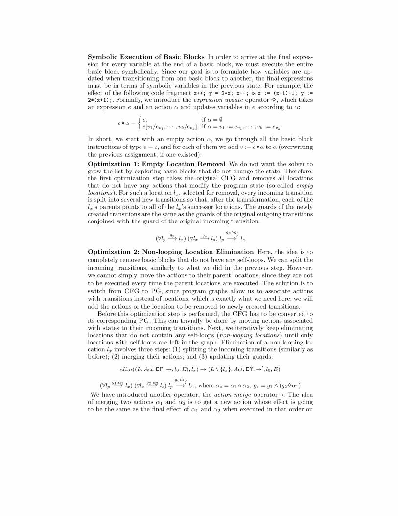
Symbolic Execution of Basic Blocks In order to arrive at the final expres-sion for every variable at the end of a basic block, we must execute the entirebasic block symbolically. Since our goal is to formulate how variables are up-dated when transitioning from one basic block to another, the final expressionsmust be in terms of symbolic variables in the previous state. For example, theeffect of the following code fragment x++; y = 2*x; x--; is x := (x+1)-1; y :=

2*(x+1);. Formally, we introduce the expression update operator G, which takesan expression e and an action α and updates variables in e according to α:

eGα =

{e, if α = ∅e[v1/ev1 , · · · , vk/evk ], if α = v1 := ev1 , · · · , vk := evk

In short, we start with an empty action α, we go through all the basic blockinstructions of type v = e, and for each of them we add v := eGα to α (overwritingthe previous assignment, if one existed).

Optimization 1: Empty Location Removal We do not want the solver togrow the list by exploring basic blocks that do not change the state. Therefore,the first optimization step takes the original CFG and removes all locationsthat do not have any actions that modify the program state (so-called emptylocations). For such a location lx, selected for removal, every incoming transitionis split into several new transitions so that, after the transformation, each of thelx’s parents points to all of the lx’s successor locations. The guards of the newlycreated transitions are the same as the guards of the original outgoing transitionsconjoined with the guard of the original incoming transition:

(∀lpgp−→ lx) (∀lx

gs−→ ls) lp

gp∧gs−→′ ls

Optimization 2: Non-looping Location Elimination Here, the idea is tocompletely remove basic blocks that do not have any self-loops. We can split theincoming transitions, similarly to what we did in the previous step. However,we cannot simply move the actions to their parent locations, since they are notto be executed every time the parent locations are executed. The solution is toswitch from CFG to PG, since program graphs allow us to associate actionswith transitions instead of locations, which is exactly what we need here: we willadd the actions of the location to be removed to newly created transitions.

Before this optimization step is performed, the CFG has to be converted toits corresponding PG. This can trivially be done by moving actions associatedwith states to their incoming transitions. Next, we iteratively keep eliminatinglocations that do not contain any self-loops (non-looping locations) until onlylocations with self-loops are left in the graph. Elimination of a non-looping lo-cation lx involves three steps: (1) splitting the incoming transitions (similarly asbefore); (2) merging their actions; and (3) updating their guards:

elim((L,Act,Eff,→, l0, E), lx) 7→ (L \ {lx}, Act,Eff,→′, l0, E)

(∀lpg1:α1−→ lx) (∀lx

g2:α2−→ ls) lpg◦:α◦

−→′ ls , where α◦ = α1 ◦ α2, g◦ = g1 ∧ (g2Gα1)

We have introduced another operator, the action merge operator ◦. The ideaof merging two actions α1 and α2 is to get a new action whose effect is goingto be the same as the final effect of α1 and α2 when executed in that order on

any variable evaluation η: Eff(α1 ◦α2, η) 7→ Eff(α2,Eff(α1, η)). In terms of mergingactions α1 and α2, expressions in α2 refer to the state after α1 has been executed,therefore, it would be incorrect to simply append α2 to α1. Instead, α2 has to beupdated first (? operator in the listing below) so that for each variable assignmentv2 := e2 in α2, expression e2 is updated with respect to α1 (e2Gα1). Once α2 hasbeen updated, the result of the merge operation is the updated α2 appended withvariable assignments in α1 that do not already appear in it. A similar intuitionholds for updating transition conditions, it is not correct to simply conjoin g1and g2, instead, g2 has to be updated first.

α ? β =

{∅, if α = ∅{v := evGβ} ∪ (α \ {v := ev}) ? β, if ∃(v := ev) ∈ α

α1 ◦ α2 = (α1 \ α2) ∪ (α2 ? α1)

Figure 3(c) shows the PG for the “Simple While” example, after all non-loopinglocations have been eliminated. First, the action i:=i+1 from the state with id=1

is moved to its incoming transitions c0, c1, c2, and c6. Next, the location withx:=x+2 action is eliminated, and as a result, edges c2 and c6 are redirected andupdated to include the x:=x+2 action.

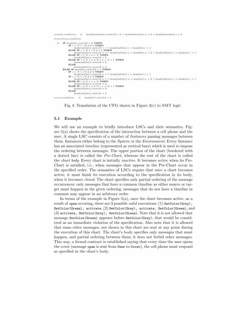
4.5 Translation of PG to SMT

Figure 4 shows the actual translation of the PG in Figure 3(c) to initial, transi-tion, and error conditions, needed for the template SMT context given in Fig-ures 1 and 2. The translation is pretty straightforward. An extra field, stateId,is first added to the state tuple to identify the current location. In this case, thestate consists of 3 variables: stateId, x, i (the variable N is constant so it is keptoutside of the state tuple). The initial condition is a direct representation of thestate in the entry block. The error condition is also easy to formulate, since all er-ror states are explicitly known upon the CFG creation. The transition conditioncontains two big nested if-then-else statements. The outer if-then-else has a casefor every non-leaf location. Inside each such case, there is an inner if-then-elsethat has a case for each of the location’s outgoing transition, where it specifieshow the state is updated when that transition is taken.

Finally, we need to define the set of possible values for the input variable N(e.g., N > 0 ∧N ≤ 10). This additional constraint is necessary because integersare unbounded in SMT theories. Recall that this technique effectively simulatesprogram loops inside SMT. Since the value of N influences the number of loopiterations, if a bound is not provided for N , the solver will try to simulate theloop for all possible values of N , and thus never terminate.

5 Execution of Live Sequence Charts

In this section we show how this model-checking technique can be applied toa non-trivial biological model-checking problem. We use the theory of lists toencode Live Sequence Charts and then run Z3 to analyze and execute them.

initial condition ≡ head(statesList).stateId = 0 ∧ head(statesList).x = 0 ∧ head(statesList).i = 0

transition condition

≡ IF head(lst).stateId = 0 THENIF i < N ∧ i % 2 6= 0 THEN

head(tail(lst)).stateId = 1 ∧ head(tail(lst)).i = head(lst).i + 1ELSE IF i < N ∧ i % 2 = 0 THEN

head(tail(lst)).stateId = 1 ∧ head(tail(lst)).x = head(lst).x + 2 ∧ head(tail(lst)).i = head(lst).i + 1ELSE IF i ≥ N ∧ x = N THEN

head(tail(lst)).stateId = 2ELSE IF i ≥ N ∧ x 6= N ∧ x = N + 1 THEN

head(tail(lst)).stateId = 2ELSE

head(tail(lst)).stateId = 3ELSE IF head(lst).stateId = 1 THEN

IF i < N ∧ i % 2 6= 0 THENhead(tail(lst)).stateId = 1 ∧ head(tail(lst)).i = head(lst).i + 1

IF i < N ∧ i % 2 = 0 THENhead(tail(lst)).stateId = 1 ∧ head(tail(lst)).x = head(lst).x + 2 ∧ head(tail(lst)).i = head(lst).i + 1

ELSE IF i ≥ N ∧ x = N THENhead(tail(lst)).stateId = 2

ELSE IF i ≥ N ∧ x 6= N ∧ x = N + 1 THENhead(tail(lst)).stateId = 2

ELSEhead(tail(lst)).stateId = 3

error condition ≡ head(lst).stateId = 3

Fig. 4: Translation of the CFG shown in Figure 3(c) to SMT logic

5.1 Example

We will use an example to briefly introduce LSCs and their semantics. Fig-ure 5(a) shows the specification of the interaction between a cell phone and theuser. A single LSC consists of a number of Instances passing messages betweenthem. Instances either belong to the System or the Environment. Every Instancehas an associated timeline (represented as vertical bars) which is used to imposethe ordering between messages. The upper portion of the chart (bordered witha dotted line) is called the Pre-Chart, whereas the rest of the chart is calledthe chart body. Every chart is initially inactive. It becomes active when its Pre-Chart is satisfied, i.e., when messages that appear in the Pre-Chart occur inthe specified order. The semantics of LSCs require that once a chart becomesactive, it must finish its execution according to the specification in its body,when it becomes closed. The chart specifies only partial ordering of the messageoccurrences: only messages that have a common timeline as either source or tar-get must happen in the given ordering; messages that do not have a timeline incommon may appear in an arbitrary order.

In terms of the example in Figure 5(a), once the chart becomes active, as aresult of open occuring, there are 3 possible valid executions: (1) SetColor(Grey),SetColor(Green), activate, (2) SetColor(Grey), activate, SetColor(Green), and(3) activate, SetColor(Grey), SetColor(Green). Note that it is not allowed thatmessage SetColor(Green) appears before SetColor(Grey), that would be consid-ered as an immediate violation of the specification. Also note that it is allowedthat some other messages, not shown in this chart are sent at any point duringthe execution of this chart. The chart’s body specifies only messages that musthappen, and partial ordering between them, it does not forbid other messages.This way, a formal contract is established saying that every time the user opensthe cover (message open is sent from User to Cover), the cell phone must respondas specified in the chart’s body.

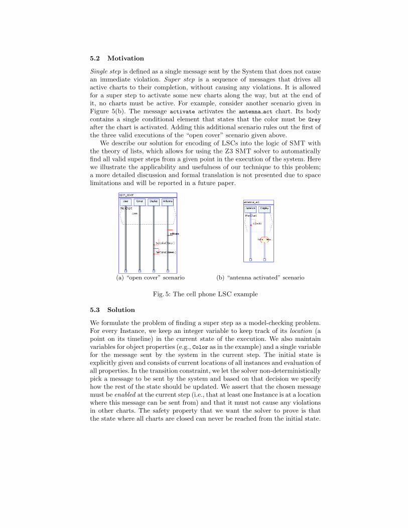
5.2 Motivation

Single step is defined as a single message sent by the System that does not causean immediate violation. Super step is a sequence of messages that drives allactive charts to their completion, without causing any violations. It is allowedfor a super step to activate some new charts along the way, but at the end ofit, no charts must be active. For example, consider another scenario given inFigure 5(b). The message activate activates the antenna act chart. Its bodycontains a single conditional element that states that the color must be Grey

after the chart is activated. Adding this additional scenario rules out the first ofthe three valid executions of the “open cover” scenario given above.

We describe our solution for encoding of LSCs into the logic of SMT withthe theory of lists, which allows for using the Z3 SMT solver to automaticallyfind all valid super steps from a given point in the execution of the system. Herewe illustrate the applicability and usefulness of our technique to this problem;a more detailed discussion and formal translation is not presented due to spacelimitations and will be reported in a future paper.

(a) “open cover” scenario (b) “antenna activated” scenario

Fig. 5: The cell phone LSC example

5.3 Solution

We formulate the problem of finding a super step as a model-checking problem.For every Instance, we keep an integer variable to keep track of its location (apoint on its timeline) in the current state of the execution. We also maintainvariables for object properties (e.g., Color as in the example) and a single variablefor the message sent by the system in the current step. The initial state isexplicitly given and consists of current locations of all instances and evaluation ofall properties. In the transition constraint, we let the solver non-deterministicallypick a message to be sent by the system and based on that decision we specifyhow the rest of the state should be updated. We assert that the chosen messagemust be enabled at the current step (i.e., that at least one Instance is at a locationwhere this message can be sent from) and that it must not cause any violationsin other charts. The safety property that we want the solver to prove is thatthe state where all charts are closed can never be reached from the initial state.

If the solver proves this property, that means that no valid super step exists.Otherwise, the solver will come back with a counter-example that contains a listof state changes, which lets us decode which message is sent at each step.

Formulating this problem using the theory of lists seems very convenient,since the number of steps needed to find a counter-example is not known inadvance. We analyzed several models of biological systems [2] and were able tofind valid super steps for systems with more than ten charts within seconds.

6 Evaluation and Results

We implemented a fully automated prototype model checker for Java programsto evaluate the idea of using the SMT theory of lists to model program traces.Currently, we support only a subset of Java programs. We used this tool to verifythe correctness of several algorithms. We also applied this technique to solve theRush Hour puzzle [1]. All experiments were conducted on a 64-bit Intel CoreDuo CPU @2.4GHz box, with 4GB of RAM, running 32-bit Windows Vista.

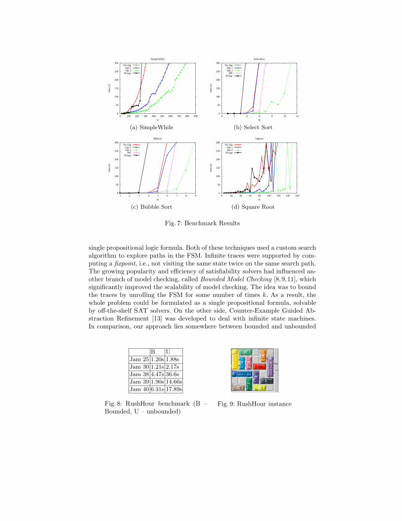
Verifying Simple Algorithms We used this technique to verify the “Simple-While” algorithm, two sorting algorithms, and the integer square root algorithmfrom Carroll Morgan’s book Programming with Specifications [22] (Figure 6).We present the comparison of verification times between the optimized and non-optimized translation for several different bounds. We compare our tool to arepresentative tool from the bounded model-checking category – JForge [16,26],and a finite model checker that doesn’t require explicit loop unrolling – JavaPathFinder [25]. The results are shown in Figure 7. The “Related Work” sectiondescribes these tools in detail and discusses the obtained results.

Non-monotonicity of some of the graphs in Figure 7 can be explained by thenature of satisfiability solvers. The solving time is highly dependent on internalheuristics (e.g., [20, 24]), so it can happen that a larger problem is solved fastersimply because the heuristics worked better (for example, it happened that alarge portion of the search space was pruned early on).

Finally, this approach performs quite efficiently when a counter-example ex-ists. For all of the presented benchmarks, our tool was able to find different(manually introduced) bugs within seconds.

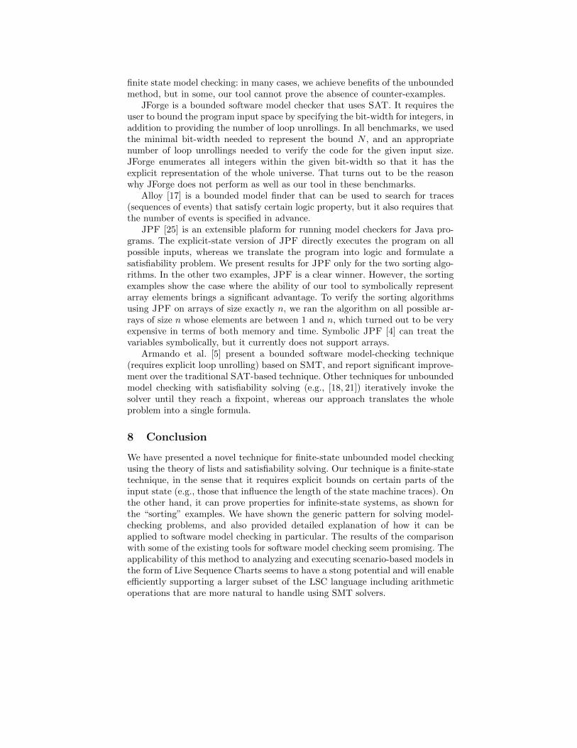
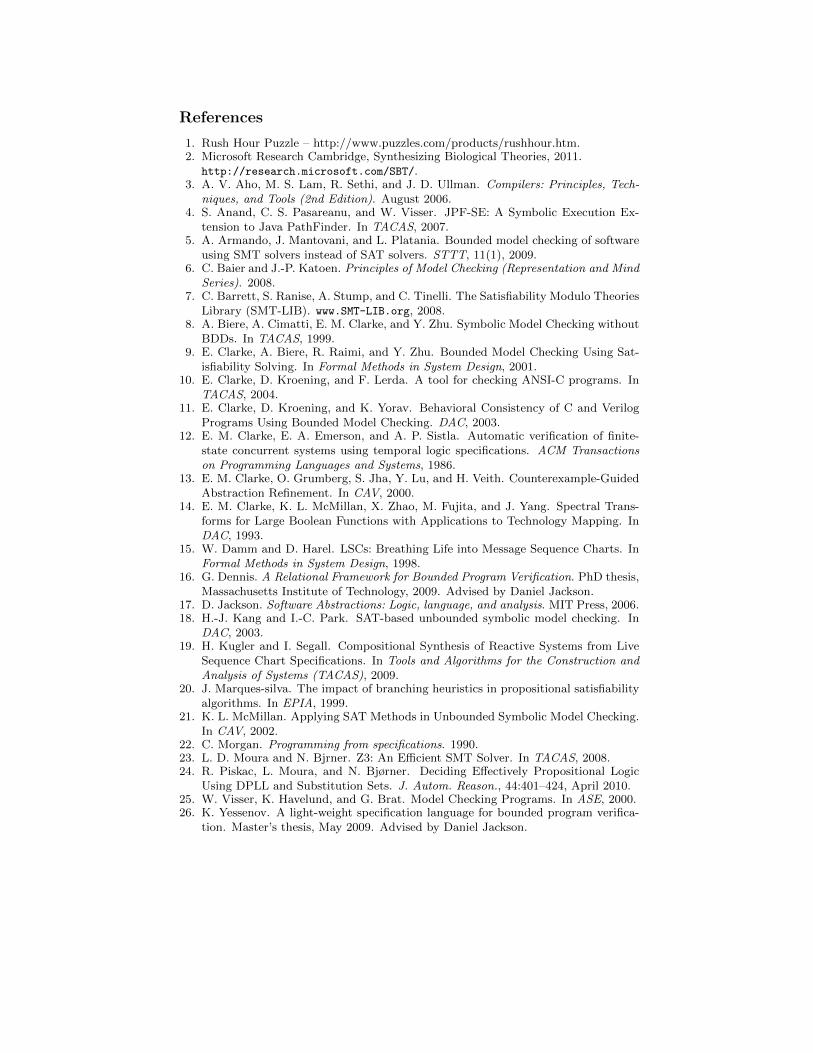
Solving the Rush Hour Puzzle RushHour is a well known puzzle where thegoal is to get the designated car (the red car in Figure 9) out of the traffic jam.This puzzle is easily expressible as a model-checking problem: the initial stateis the given configuration of cars at the starting point, the transition functionconstrains the allowed movements of the cars so that they do not crash or goover each other, and the safety property is that the red car can never reach thefar right side of the stage. If we find a counter-example to this model-checkingproblem, we have found the way to get the red car out of the jam.

We took several puzzles from [1] and compared the execution times of the twoapproaches: bounded (the case when we know the optimal number of steps) andunbounded with lists (Figure 8). SMT solvers are optimized to deal with largeflat formulas, so the fact that the bounded encoding currently performs better

void simpleWhile ( int N) {int x = 0 , i = 0 ;while ( i < N) {i f ( i % 2 == 0)

x += 2 ;i++;}assert x == N | | x == N + 1;}

void s e l e c t S o r t ( int [ ] a , int N) {for ( int j =0; j<N−1; j++) {int min = j ;for ( int i=j +1; i < N; i++)i f ( a [ min ] > a [ i ] ) min = i ;

int t = a [ j ] ; a [ j ] = a [ min ] ; a [ min ] = t ;}for ( int j =0; j<N−1; j++)assert a [ j ] <= a [ j +1] ;

}

void bubbleSort ( int [ ] a , int N) {for ( int j =0; j<N−1; j++)for ( int i =0; i<N−j−1; i++)i f ( a [ i ] > a [ i +1]) {

int t = a [ i ] ;a [ i ] = a [ i +1] ;a [ i +1] = t ;

}for ( int j =0; j<N−1; j++)assert a [ j ] <= a [ j +1] ;

}

int intSqRoot ( int N) {int r = 1 , q = N;while ( r+1 < q) {

int p = ( r+q) / 2 ;i f (N < p∗p) q = p ;else r = p ;

}assert r∗ r <= N && ( r+1)∗( r+1)>N;return r ;

}

Fig. 6: Benchmark Algorithms

does not come as a surprise. However, we were able to solve the most difficultpuzzles (e.g., Jam 38-40 require more than thirty steps) within a minute.

This problem is quite different from the software model-checking problems,because at every step, there are typically several available valid moves, so atevery step, the solver has to non-deterministically decide which move to takein order to finally reach an error state (this never happens in software modelchecking if programs are deterministic). This puzzle is a typical example of howthis technique can be used to solve planning problems without bounding thenumber of steps in advance.

One limitation of our current implementation is that it is not able to prove itif the solution does not exist. The solver gets stuck exploring the same states overand over again (e.g., moving the red car back and forth between the neighboringcells). However, if a solution exists, this problem is not manifested. Also notethat this does not happen in software model checking if the target programalways terminates. An obvious solution is to forbid the same states to appearin the states list. This additional constraint is expressible in SMT logic, but inpractice it does not perform that well. Instead, we believe that the SMT solvercould be tweaked so that it internally knows that while building the states listit should never include the same state twice in a single search path. It would bevery efficient to implement this inside the solver, because the state is representedexplicitly inside list elements, so it would be easy to compare states for equality.

7 Related Work

Model checking was originally defined as a technique for proving properties aboutFinite State Machines (FSM) [12]. The pioneering tools had used an explicit rep-resentation of the entire state graph, which led to what is known as the stateexplosion problem. To mitigate that problem, Binary Decision Diagrams (BDD)were introduced by McMillan [14] to symbolically represent a set of states with a

0

50

100

150

200

250

300

0 100 200 300 400 500 600 700 800 900

time

(s)

N

SimpleWhile

No OptOpt 1Opt 2

JForge

(a) SimpleWhile

0

50

100

150

200

250

300

0 2 4 6 8 10 12

time

(s)

N

SelectSort

No OptOpt 1Opt 2

JPFJForge

(b) Select Sort

0

50

100

150

200

250

300

1 2 3 4 5 6 7 8 9

time

(s)

N

BblSort

No OptOpt 1Opt 2

JPFJForge

(c) Bubble Sort

0

50

100

150

200

250

300

0 20 40 60 80 100 120 140 160

time

(s)

N

SqRoot

No OptOpt 1Opt 2

JForge

(d) Square Root

Fig. 7: Benchmark Results

single propositional logic formula. Both of these techniques used a custom searchalgorithm to explore paths in the FSM. Infinite traces were supported by com-puting a fixpoint, i.e., not visiting the same state twice on the same search path.The growing popularity and efficiency of satisfiability solvers had influenced an-other branch of model checking, called Bounded Model Checking [8,9,11], whichsignificantly improved the scalability of model checking. The idea was to boundthe traces by unrolling the FSM for some number of times k. As a result, thewhole problem could be formulated as a single propositional formula, solvableby off-the-shelf SAT solvers. On the other side, Counter-Example Guided Ab-straction Refinement [13] was developed to deal with infinite state machines.In comparison, our approach lies somewhere between bounded and unbounded

B U

Jam 25 1.20s 1.88s

Jam 30 1.21s 2.17s

Jam 38 4.47s 36.6s

Jam 39 1.90s 14.66s

Jam 40 6.31s 17.89s

Fig. 8: RushHour benchmark (B –Bounded, U – unbounded)

Fig. 9: RushHour instance

finite state model checking: in many cases, we achieve benefits of the unboundedmethod, but in some, our tool cannot prove the absence of counter-examples.

JForge is a bounded software model checker that uses SAT. It requires theuser to bound the program input space by specifying the bit-width for integers, inaddition to providing the number of loop unrollings. In all benchmarks, we usedthe minimal bit-width needed to represent the bound N , and an appropriatenumber of loop unrollings needed to verify the code for the given input size.JForge enumerates all integers within the given bit-width so that it has theexplicit representation of the whole universe. That turns out to be the reasonwhy JForge does not perform as well as our tool in these benchmarks.

Alloy [17] is a bounded model finder that can be used to search for traces(sequences of events) that satisfy certain logic property, but it also requires thatthe number of events is specified in advance.

JPF [25] is an extensible plaform for running model checkers for Java pro-grams. The explicit-state version of JPF directly executes the program on allpossible inputs, whereas we translate the program into logic and formulate asatisfiability problem. We present results for JPF only for the two sorting algo-rithms. In the other two examples, JPF is a clear winner. However, the sortingexamples show the case where the ability of our tool to symbolically representarray elements brings a significant advantage. To verify the sorting algorithmsusing JPF on arrays of size exactly n, we ran the algorithm on all possible ar-rays of size n whose elements are between 1 and n, which turned out to be veryexpensive in terms of both memory and time. Symbolic JPF [4] can treat thevariables symbolically, but it currently does not support arrays.

Armando et al. [5] present a bounded software model-checking technique(requires explicit loop unrolling) based on SMT, and report significant improve-ment over the traditional SAT-based technique. Other techniques for unboundedmodel checking with satisfiability solving (e.g., [18, 21]) iteratively invoke thesolver until they reach a fixpoint, whereas our approach translates the wholeproblem into a single formula.

8 Conclusion

We have presented a novel technique for finite-state unbounded model checkingusing the theory of lists and satisfiability solving. Our technique is a finite-statetechnique, in the sense that it requires explicit bounds on certain parts of theinput state (e.g., those that influence the length of the state machine traces). Onthe other hand, it can prove properties for infinite-state systems, as shown forthe “sorting” examples. We have shown the generic pattern for solving model-checking problems, and also provided detailed explanation of how it can beapplied to software model checking in particular. The results of the comparisonwith some of the existing tools for software model checking seem promising. Theapplicability of this method to analyzing and executing scenario-based models inthe form of Live Sequence Charts seems to have a stong potential and will enableefficiently supporting a larger subset of the LSC language including arithmeticoperations that are more natural to handle using SMT solvers.

References

1. Rush Hour Puzzle – http://www.puzzles.com/products/rushhour.htm.2. Microsoft Research Cambridge, Synthesizing Biological Theories, 2011.

http://research.microsoft.com/SBT/.3. A. V. Aho, M. S. Lam, R. Sethi, and J. D. Ullman. Compilers: Principles, Tech-

niques, and Tools (2nd Edition). August 2006.4. S. Anand, C. S. Pasareanu, and W. Visser. JPF-SE: A Symbolic Execution Ex-

tension to Java PathFinder. In TACAS, 2007.5. A. Armando, J. Mantovani, and L. Platania. Bounded model checking of software

using SMT solvers instead of SAT solvers. STTT, 11(1), 2009.6. C. Baier and J.-P. Katoen. Principles of Model Checking (Representation and Mind

Series). 2008.7. C. Barrett, S. Ranise, A. Stump, and C. Tinelli. The Satisfiability Modulo Theories

Library (SMT-LIB). www.SMT-LIB.org, 2008.8. A. Biere, A. Cimatti, E. M. Clarke, and Y. Zhu. Symbolic Model Checking without

BDDs. In TACAS, 1999.9. E. Clarke, A. Biere, R. Raimi, and Y. Zhu. Bounded Model Checking Using Sat-

isfiability Solving. In Formal Methods in System Design, 2001.10. E. Clarke, D. Kroening, and F. Lerda. A tool for checking ANSI-C programs. In

TACAS, 2004.11. E. Clarke, D. Kroening, and K. Yorav. Behavioral Consistency of C and Verilog

Programs Using Bounded Model Checking. DAC, 2003.12. E. M. Clarke, E. A. Emerson, and A. P. Sistla. Automatic verification of finite-

state concurrent systems using temporal logic specifications. ACM Transactionson Programming Languages and Systems, 1986.

13. E. M. Clarke, O. Grumberg, S. Jha, Y. Lu, and H. Veith. Counterexample-GuidedAbstraction Refinement. In CAV, 2000.

14. E. M. Clarke, K. L. McMillan, X. Zhao, M. Fujita, and J. Yang. Spectral Trans-forms for Large Boolean Functions with Applications to Technology Mapping. InDAC, 1993.

15. W. Damm and D. Harel. LSCs: Breathing Life into Message Sequence Charts. InFormal Methods in System Design, 1998.

16. G. Dennis. A Relational Framework for Bounded Program Verification. PhD thesis,Massachusetts Institute of Technology, 2009. Advised by Daniel Jackson.

17. D. Jackson. Software Abstractions: Logic, language, and analysis. MIT Press, 2006.18. H.-J. Kang and I.-C. Park. SAT-based unbounded symbolic model checking. In

DAC, 2003.19. H. Kugler and I. Segall. Compositional Synthesis of Reactive Systems from Live

Sequence Chart Specifications. In Tools and Algorithms for the Construction andAnalysis of Systems (TACAS), 2009.

20. J. Marques-silva. The impact of branching heuristics in propositional satisfiabilityalgorithms. In EPIA, 1999.

21. K. L. McMillan. Applying SAT Methods in Unbounded Symbolic Model Checking.In CAV, 2002.

22. C. Morgan. Programming from specifications. 1990.23. L. D. Moura and N. Bjrner. Z3: An Efficient SMT Solver. In TACAS, 2008.24. R. Piskac, L. Moura, and N. Bjørner. Deciding Effectively Propositional Logic

Using DPLL and Substitution Sets. J. Autom. Reason., 44:401–424, April 2010.25. W. Visser, K. Havelund, and G. Brat. Model Checking Programs. In ASE, 2000.26. K. Yessenov. A light-weight specification language for bounded program verifica-

tion. Master’s thesis, May 2009. Advised by Daniel Jackson.