Embed Size (px)
Citation preview
Model-Free International SDFs in Incomplete Markets∗
Mirela Sandulescu† Fabio Trojani ‡ Andrea Vedolin §
August 2017
Abstract
We characterize model-free international stochastic discount factors (SDFs) undervarious degrees of market segmentation in incomplete markets. Our SDFs can befactorized into permanent and transitory components and they minimize the SDFdispersion subject to international pricing constraints. We find that large permanentSDF components are essential to jointly reconcile the low exchange rate volatility,the exchange rate cyclicality and the forward premium anomaly, however, at the costof highly volatile SDFs. Market segmentation in stock and bond markets inducesa deviation from the asset market view which helps avoid implausibly large SDFdispersions. Hence, economies featuring some form of mild market segmentation andlarge martingale components can match salient features of exchange rates, bond,equity, and FX option markets.
Keywords: stochastic discount factor, exchange rates, market segmentation, market incom-
pleteness.
First Version: November 2016
∗We thank Federico Gavazzoni, Anna Pavlova, Alireza Tahbaz-Salehi, Raman Uppal and conference partic-ipants at the International Conference of the French Finance Association (Valence), SoFiE Annual Meeting atNYU, and International Finance Conference at Cass Business School for helpful comments. All errors are ours.†SFI and University of Lugano, Department of Economics, Email: [email protected]‡SFI and University of Geneva, School of Economics and Management & GFRI, Email:
[email protected]§Boston University, Department of Finance, Email: [email protected]
The simplest canonical models in international finance are at odds with many salient features
of exchange rates and international asset prices. These can be summarized in three asset
pricing puzzles: the low exchange rate volatility documented by Obstfeld and Rogoff (2001) and
Brandt, Cochrane, and Santa-Clara (2006), the counter-cyclicality puzzle of Kollmann (1991)
and Backus and Smith (1993), and the forward premium anomaly of Hansen and Hodrick (1980)
and Fama (1984).
These puzzles have been the subject of many studies both theoretically and empirically.
One strand of the literature assumes integrated complete markets under various specifications
of preferences and consumption dynamics. Another strand of the literature questions the as-
sumption of financial market completeness and argues that some form of incompleteness is
useful to accomodate the puzzling features of exchange rates. Recently, Lustig and Verdelhan
(2016) conclude, however, that the three puzzles cannot be jointly explained in an international
consumption CAPM setting even under incomplete spanning.1
In complete markets, the rate of appreciation of the real exchange rate equals the ratio
of the foreign and domestic stochastic discount factors (SDFs): X = Mf/Md, i.e. the asset
market view of exchange rates holds. The common understanding in international financial
economics is that under incomplete markets, the real exchange rate is in general different from
this ratio. Such deviation from the asset market view of exchange rates can be captured by a
multiplicative stochastic wedge as in Backus, Foresi, and Telmer (2001).
In this paper, we develop a parsimonious model-free approach to characterize theoretically
and to measure empirically the relations between international SDFs, exchange rate puzzles
and deviations from the market view of exchange rates. We develop our theory and empirical
evidence for economies where domestic and foreign investors have access to short- and long-
term bonds and stocks. In order to characterize international SDFs without committing to a
particular asset pricing model, we estimate different projections of international SDFs on the
1The complete market assumption is used in the habit model of Stathopoulos (2017) to generate sizablecurrency risk premia. Similarly, Colacito and Croce (2013) employ recursive preferences with highly correlatedinternational martingale components in a two-country complete market setting. Farhi and Gabaix (2016) rely ona complete market economy with time-additive preferences and a time-varying probability of rare consumptiondisasters. Gabaix and Maggiori (2015) provide a theory of exchange rate determination based on capital flowsin financial markets with heterogenous trading technologies, while Chien, Lustig, and Naknoi (2015) propose atwo-country stochastic growth model with segmented financial markets that generates smooth exchange ratesand highly volatile stochastic discount factors.
space of tradable returns for domestic and foreign investors.
Given the multitude of SDFs pricing returns in incomplete markets, we explore minimum
dispersion SDFs, which minimize different notions of variability, e.g., the Hansen and Jagan-
nathan (1991) SDF when we minimize the SDF variance. Additionally, we focus on minimum
entropy SDF projections, as well as on a third SDF projection that minimizes the SDF Hellinger
divergence. Each of these dispersion measures has appealing features for the purpose of our
analysis. First, we show that minimum Hellinger divergence SDFs place a sharp dispersion
bound on the first moment of transient SDF components. Second, we prove that minimum en-
tropy SDFs always imply the validity of the asset market view whenever foreign and domestic
investors trade the same set of assets in integrated markets. In contrast, a stochastic wedge
usually arises with respect to any other minimum dispersion SDF, including tradable minimum
variance SDFs. Therefore, we establish that the exchange rate wedge is always interpretable
as a measure of the amount of untraded exchange rate risk in integrated international financial
markets.
Consistent with the low exchange rate volatility puzzle, a deviation from the asset market
view intuitively embeds a weaker degree of similarity or co-movement between international
SDFs. Motivated by this observation, earlier literature studies the amount of risk-sharing in
complete markets (see, e.g., Brandt, Cochrane, and Santa-Clara (2006) and Chabi-Yo and
Colacito (2017)). In this paper, we measure SDF similarity using a novel similarity index,
which takes into account the whole SDF distribution and can be computed from at-the-money
exchange rate option prices alone whenever the asset market view holds. Using this index, we
quantify empirically the degree of SDF dissimilarity under various forms of deviation from the
asset market view in our setting.
Using our model-free SDFs, we study the implications of different deviations from market
symmetry, from fully disconnected domestic and foreign markets to highly integrated markets,
in which (risk-free) short- and long-term bonds and stocks are traded internationally. Hence,
we quantify the trade-offs between a larger domestic and foreign SDF dispersion necessary to
price a wider set of returns, the three exchange rate puzzles and a deviation from the asset view.
For our empirical analysis, we adopt the insights of Bansal and Lehmann (1997) and Alvarez
and Jermann (2005) and identify the transient component of domestic and foreign SDFs using
2
long-term bonds. In this way, we force our preference-free SDF projections to correctly price
the returns of long-maturity bonds in the local currency, which is the most natural way to
empirically identify the short- and long-run SDF components.
In the empirical study we consider eight benchmark currencies, namely the US dollar, the
British pound, the Swiss franc, the Japanese yen, the euro (Deutsche mark before the intro-
duction of the euro), the Australian dollar, the Canadian dollar and the New Zealand dollar.
The resulting seven exchange rates are expressed with respect to the US dollar as the domestic
currency and the sample period spans January 1975 to December 2015. We summarize our
empirical findings as follows.
Firstly, we document that our main empirical results are largely independent of the par-
ticular choice of SDF projection used. Irrespective of the degree of market segmentation, we
find that permanent (martingale) components of domestic and foreign SDFs across markets are
all highly volatile, to the point that they actually dominate the overall SDF variability. The
co-movement between transient and permanent SDF components is negative, in order to match
the typically negative local risk premia of long-term bonds. These features are consistent with
previous evidence for the US market in, e.g., Alvarez and Jermann (2005).
Our starting point for our empirical investigation is incomplete but fully integrated interna-
tional bonds and stock markets. We find that irrespective of the choice of minimum dispersion
SDFs, the untradable component of exchange rate risk explains only a small fraction of the
exchange rate variability. Therefore, deviations from the asset market view of exchange rates
are uniformly small in these settings, giving rise to almost perfectly co-moving international
SDFs that imply a high level of SDF dispersion.
We find that whenever investors are allowed to trade internationally the riskless short-term
bonds, the ensuing minimum dispersion SDFs jointly address the three exchange rate puzzles.
The low exchange rate volatility is explained by means of a volatile wedge between exchange
rates and the ratio of foreign and domestic SDFs. The cyclicality puzzle is addressed because
cross-country differences in observable transient SDF components are only weakly related to
exchange rate returns. Carry trade premia are also in line with those observed in the data,
because the international pricing constraints on risk-free bonds effectively force domestic and
foreign SDFs to correctly reproduce the cross-section of currency risk premia.
3
When successively opening international markets to long-term bond and stock trading, the
three exchange rate puzzles are still explained, by construction. Additionally, we find that
the SDF dispersions in integrated long-term bond and stock markets are significantly larger
than under integrated short-term bond markets alone. These increases in SDF dispersion are
necessary in order to match the cross-section of international equity premia, as well as long-term
bond risk premia. For instance, compared to the case of integrated short-term bond markets,
the increase in minimum variance SDFs dispersion is on average 30%, the highest values being
encountered especially for the funding currencies. These large SDF dispersions suggest that
it may be difficult to explain exchange rate puzzles using structural asset pricing models with
traded domestic equity and fully integrated international long-term bond and equity markets.
Finally, the exchange rate wedge vanishes for the minimum entropy SDFs and is negligible for
the minimum variance and Hellinger SDFs, leading to almost perfectly correlated domestic and
foreign pricing kernels.
Lastly, we introduce a novel measure to quantify the similarity between international SDFs.
The index extends traditional measures of SDF covariance or co-dependence, since it quantifies
how similar the distributions of the domestic and foreign SDFs are. We find that on average,
in integrated symmetric markets, the estimates are almost one. There are, however, cross-
sectional differences and the SDFs appear to be more dissimilar during crisis periods. Market
segmentation lowers the degree of similarity.
We contrast our findings with the international risk sharing index of Chabi-Yo and Colacito
(2017) and the inference we draw is consistent: in asymmetric settings, roughly 50% of financial
risks are being shared, whereas as one moves towards symmetry, international risk sharing
is perfect. The latter is a direct consequence of the fact that the asset market view holds
for minimum entropy SDFs, whereas deviations from it are small for the other dispersion
measures. As such, we document that there is a trade-off between similarity, SDF dispersion
and international financial risk sharing. Hence, international bond or stock market segmentation
appears a useful assumption for structural models of exchange rate determination, in which a
deviation from the asset market view always arises.
After a literature review, the rest of the paper is organized as follows. Section 1 provides the
theoretical framework for our model-free selection of minimum dispersion SDFs in international
4
financial markets. Section 2 describes our data and our main empirical findings, under various
benchmark assumptions about the degree of international market segmentation. Section 3
concludes and discusses directions for future research.
Literature Review: Our paper contributes to the literature that studies the ability of
market incompleteness to address various puzzles in international finance. Bakshi, Cerrato,
and Crosby (2015) and Lustig and Verdelhan (2016) study preference-free SDFs in incomplete
markets to address the weak link between exchange rates and macroeconomic fundamentals.
The former impose “good deal” bounds on international SDFs to examine economies with a low
amount of risk sharing and economically motivated pricing errors. Lustig and Verdelhan (2016)
introduce a stochastic wedge between foreign and domestic SDFs and conclude that incomplete
markets cannot jointly address the three exchange rate puzzles under a Consumption-CAPM
framework. In our paper, we characterize the properties of international SDFs without in-
troducing any particular distributional assumption, while allowing SDFs to be factorized into
transient and permanent components. We demonstrate that this factorization is key to recon-
cile stylized exchange rate facts, especially the Backus-Smith puzzle. We further highlight the
distinct economic roles of minimum entropy and minimum variance SDFs with respect to the
asset market view in symmetric incomplete international markets.
Another strand of literature studies structural models of exchange rate determination under
different assumptions about market segmentation. Chien, Lustig, and Naknoi (2015) show that
while limited stock market participation can reconcile highly correlated international SDFs
with a low correlation in consumption growth, it is less successful in addressing the Backus
and Smith puzzle. Alvarez, Atkeson, and Kehoe (2009) explain the Backus and Smith puzzle
in a general equilibrium model with financial frictions and endogenous market participation.
Gabaix and Maggiori (2015) study the disconnect puzzle and violations of UIP in a setting where
financial intermediaries face frictions in segmented markets. We contribute to this literature by
documenting with a model-free approach the large dispersion trade-offs implied by settings with
fully integrated international financial markets. We also quantify the implications of various
degrees of market segmentation in international bond and stock markets. Theoretically, we
show that the asset market view of exchange rates always holds for minimum entropy SDFs in
symmetric international markets, independent of the degree of incompleteness. As a byproduct,
5
we empirically document that minimum dispersion domestic and foreign SDFs are always highly
correlated in symmetric, even if incomplete, market settings. Consistently with Burnside and
Graveline (2012), among others, the asset market view of exchange rates does not hold in general
for minimum variance SDFs. We provide a general economic interpretation of this feature, by
decomposing the wedge between exchange rates and minimum variance SDF ratios in terms of
tradable and untradable exchange rate risks in international asset markets.
Maurer and Tran (2016) construct minimum variance SDF projections on excess returns
in incomplete continuous-time models, showing that the asset market view holds if and only
if exchange rate risks can be disentangled in symmetric domestic and foreign asset markets,
i.e. only in the absence of jump risk. Our approach is different and explicitly considers var-
ious model-free SDFs projections. This allows us to show that the asset market view always
holds for minimum entropy SDFs in symmetric economies, irrespective of the degree of market
incompleteness and without making any additional assumptions on the distribution of asset re-
turns. Similarly, considering different admissible SDF projections is key to be able to decompose
exchange rate risks in tradable and untradable components.
The SDF factorization in permanent and transient components has been employed previ-
ously in various studies of international asset pricing under a complete markets assumption.
Chabi-Yo and Colacito (2017) make use of co-entropies to characterize the horizon properties
of SDFs co-movement. Lustig, Stathopoulos, and Verdelhan (2016) examine the international
bond premia and conclude that the bond return parity condition holds when nominal exchange
rates are stationary. The large co-movement of permanent components in their studies is a
natural consequence of the underlying completeness assumption. We show that a large co-
movement of permanent SDFs components emerges in all symmetric international economies in
our study, regardless of their different degree of market incompleteness. For minimum entropy
SDFs, this is a direct implication of the fact that the asset market view theoretically holds in
this case. For minimum variance SDFs, this follows from the fact that the estimated fraction
of untradable exchange rate risk in symmetric economies is rather small. However, we also find
that the underlying SDF dispersion when bonds or stocks are traded internationally is probably
difficult to explain using structural complete market models.
6
1 Preference-Free SDFs in Incomplete International Markets
In this section, we introduce our model-free methodology for identifying minimum dispersion
SDFs in incomplete domestic and foreign financial markets. One motivation for using minimum
dispersion SDFs relies on the fact that they can be understood as optimal SDF projections
generated by traded asset returns which also naturally bound the welfare attainable by marginal
investors. In this sense, minimum dispersion SDFs constrain the best deals attainable by
domestic and foreign investors. Moreover, minimum dispersion SDFs directly imply model-free
constraints on the distribution of asset returns, such as asset pricing bounds on expected (log)
returns and Sharpe ratios. These constraints need to be satisfied by any admissible international
asset pricing model. We focus on three types of SDFs which can be obtained by minimizing
the SDF entropy, variance, and Hellinger divergence.
We denote by Md and Mf generic domestic and foreign SDFs that price a vector of returns
Rd and Rf from the perspective of domestic and foreign investors, i.e., in the domestic and
foreign currency, respectively. Moreover, we denote by X the gross exchange rate return, where
the exchange rate is defined as the domestic currency price of one unit of the foreign currency.
In the following, we generally work with real SDFs, returns, and exchange rates. Whenever we
use nominal exchange rates, we state this explicitly. We first introduce two key concepts that
are central to our work.
Definition 1. (i) International financial markets are called symmetric whenever span(Rd) =span(RfX), where span(Rd) (span(RfX)) is the linear span of portfolio returns generated bydomestic returns (foreign returns converted in domestic currency). (ii) The asset marketview of exchange rates is said to hold with respect to SDFs Md and Mf if
X = Mf/Md .
By definition, symmetric financial markets are integrated international financial markets, in
which each foreign return is tradable by domestic investors through exchange rate markets, and
vice versa. Consistent with this definition, we interpret a deviation from market symmetry as a
particular form of market segmentation. One implication of market symmetry is that whenever
domestic and foreign markets are complete, the asset market view of exchange rates holds. In
this setting, there exists a unique SDF that can be expressed in different currency units by
a simple change of numeraire via the exchange rate return. In other words, in complete and
7
symmetric markets, domestic and foreign SDFs are numeraire invariant.
In incomplete or partially segmented markets a deviation from the asset market view can
arise, which renders the relation between domestic and foreign SDFs generally more complex.
In principle, such a breakdown of the asset market view can be a pervasive feature that makes
minimum dispersion SDFs not numeraire invariant in such settings. We show, however, that
minimum entropy SDFs preserve their numeraire invariance even under incomplete markets,
implying that the asset market view always holds under market symmetry for these SDFs. This
property does not hold for any other minimum dispersion SDF. Therefore, symmetric market
settings are a natural benchmark to measure deviations from the market view in our context.
Finally, we specify a new family of model-free indices of SDF similarity, which help us to
quantify the trade-offs between a deviation from the asset market view and the amount of
international SDF dispersion. These indices can be computed from observed exchange rate
option prices and deliver model-free benchmarks for the similarity of international SDFs under
different market structures.
1.1 Minimum-Dispersion SDFs
As is well known, stochastic discount factors can be thought of as investors’ marginal utility of
wealth. Using a preference-free approach, we study the properties of these SDFs in incomplete
and possibly segmented markets, by restricting the set of assets that investors can trade.
The vectors of domestic and foreign returns priced by Md and Mf are Rd = (Rd0, . . . , RdKd)′
and Rf = (Rf0, . . . , RfKf)′, where Rd0 and Rf0 denote the risk-free returns in the domestic and
foreign markets. In our empirical analysis, we take the United States (US) as the domestic
market and the United Kingdom (UK), Switzerland (CH), Japan (JP ), the European Union
(EU), Australia (AU), Canada (CA) or New Zealand (NZ) as the foreign markets.2 For each
market i = d, f , we study the minimum-dispersion SDF that solves for parameter αi ∈ R\{1}
the following optimization problem:
minMi
− 1
αilogE[Mαi
i ] ,
s.t. E[MiRi] = 1 ; Mi > 0 .
(1)
2Prior to the introduction of the Euro, we take Germany in its place.
8
The pricing restriction E[MiRi] = 1 in equation (1), where 1 is a (Ki + 1)× 1 vector of ones,
ensures that the SDF satisfies the given pricing constraints, while the positivity constraint
Mi > 0 ensures that it is indeed an admissible SDF.3 The formulation in equation (1) depends
on parameter αi, which subsumes various SDF choices in incomplete markets economies. More
specifically, different values of αi assign different weights to the higher order moments of the
asset return distribution. For example, for αi = 2, we obtain the well-known minimum variance
bounds of Hansen and Jagannathan (1991), while αi = 0 (αi = 0.5) corresponds to entropy
(Hellinger) bounds. The latter two also allow us to study the robustness of our findings with
respect to the higher-order moments of the asset return distribution. In line with Almeida
and Garcia (2012), among others, the minimum-entropy (αi = 0) SDF delivers a tight upper
bound on the maximal expected log return with respect to the available traded assets, while
the minimum-variance (αi = 2) SDF delivers a tight upper bound on the maximal Sharpe ratio.
More generally, every minimum dispersion SDF corresponds to a different set of tight con-
straints on the moments of traded asset returns. Since asset returns are observable but SDFs
are not, we can conveniently restate the minimum objective function in equation (1) into the
maximum objective function in the following dual portfolio problem (see, e.g., Orlowski, Sali,
and Trojani (2016), Proposition 4):
maxλi
(αi − 1)
αilogE
[Rαi/(αi−1)λi
],
s.t. Rλi > 0 ,
(2)
where Rλi =∑Ki
k=1 λikRik + (1−∑Ki
k=1 λik)Ri0 and λik denotes the portfolio weight of asset k
in market i = d, f . The first-order conditions (FOCs) associated with optimization problem (2)
read:
E[R−1/(1−αi)λ∗i
(Rik −Ri0)]
= 0. (3)
Using the optimal return Rλ∗iin equation (2), we can now solve for the minimum dispersion
3In case the risk-free return Ri0 is traded, an equivalent formulation of problem (1) is:
minMi
− 1
αilogE[(Mi/E[Mi])
αi ] ,
s.t. E[MiRi] = 1 ; Mi > 0 .
9
SDF, M∗i , explicitly.
Proposition 1. The minimum dispersion SDF in international financial markets is given by:
M∗i = R
−1/(1−αi)λ∗i
/E[R−αi/(1−αi)λ∗i
], (4)
where Rλ∗iis the optimal portfolio return which solves the optimization problem in (2). More-
over, due to the duality relation between problems (1) and (2), we have:
− 1
αilogE[M∗αi
i ] =(αi − 1)
αilogE[R
αi/(αi−1)λ∗i
]. (5)
Proof: See Appendix.
Using different values of parameter αi, we easily obtain different minimum dispersion SDFs
via equation (5), denoted by M∗i (αi).
Example 1. For αi = 0, the minimum entropy SDF is given by:
M∗i (0) = R−1λ∗i
.
The minimum Hellinger SDF is obtained for αi = 1/2:
M∗i (1/2) = R−2λ∗i
/E(R−1λ∗i ).
Finally, for αi = 2 we retrieve the minimum variance SDF:
M∗i (2) = Rλ∗i
/E(R2λ∗i
).
Based on these SDFs, we obtain the following bound for the distribution of any traded
return Rλi :4
− 1
αilogE[Mαi
i ] ≥ (αi − 1)
αilogE[R
αi/(αi−1)λi
] . (6)
Setting αi = 0 and αi = 2, we obtain the well-known entropy and variance bounds. Additionally,
we also consider αi = 1/2, which yields the Hellinger bound:5
logE[M
1/2i
]≤
logE[R−1λi ]
2. (7)
4When there is no duality gap between the primal and dual solutions, i.e. for the optimal portfolio returnRλ∗
i, we retrieve equation (5).
5Kitamura, Otsu, and Evdokimov (2013) emphasize the optimal robustness features of Hellinger-type dis-persion measures. We later show that Hellinger bounds naturally induce tight constraints on the first momentof transitory SDF components.
10
In the following, we explore the link between deviations from the asset market view and min-
imum dispersion SDFs under various forms of departure from market symmetry. We achieve
this by adjusting the vector of traded returns Rd and Rf to reflect different degrees of financial
market segmentation, from settings of fully segmented markets to economies where domestic
investors can trade foreign bonds and stocks by resorting to exchange rate markets.
1.2 SDF Components and Exchange Rate Wedges
The persistence properties of SDFs have been shown to be important determinants of long-lived
securities such as stocks, while transient SDF components are pinned down by the dynamics of
long-term bonds. Therefore, we factorize international SDFs into martingale (permanent) and
transient components. The minimum dispersion problem (1) applies without loss of generality
when SDFs are factorized into permanent and transient components:
Mi = MPi M
Ti . (8)
In line with Alvarez and Jermann (2005), MPi is identifiable by normalization E[MP
i ] = 1,
while the transient component is the inverse of the return of the infinite maturity bond, i.e.
MTi := 1/Ri∞.6 In this setting, the normalization of the permanent component is ensured
by requiring the return on the infinite maturity bond to be priced by SDF Mi = MPi /Ri∞.
Equivalently, Ri∞ is defined as one of the components of return vector Ri in problem (1).
Tradability of Ri∞ obviously impacts the form of minimum dispersion SDFs and increases the
SDF variability.
Since inequality (7) is valid for any traded return, we obtain the following tight constraint
on the expected transient SDF component:
logE[(M∗
i (1/2))1/2]≤ logE[R−1i∞]
2. (9)
Therefore, the Hellinger minimum dispersion SDF directly reveals information about the av-
erage size of transient SDF components and vice-versa. In the following sections, we apply
6For instance, in the long run risk model with recursive preferences, the transient component is a functionof consumption growth alone, while the permanent (martingale) component is a function of the return of theclaim to total future consumption.
11
factorization (8) to quantify in a model-free way the relative importance of international tran-
sient and persistent SDF components for explaining salient features of exchange rates.
A useful property of minimum dispersion problem (1) is that it can flexibly accommodate
different forms of deviations from market symmetry, simply by adjusting the tradable returns
Rd and Rf from the perspective of domestic and foreign investors. It is well-known that
whenever international markets are complete, domestic and foreign SDFs are uniquely defined.
As a consequence, all minimum dispersion SDFs are identical. In this framework, whenever
international financial markets are symmetric, consistently with the Euler equation pricing
restrictions, the exchange rate return is uniquely given by the ratio of the foreign and domestic
SDFs, i.e., the asset market view as stated in Definition 1 holds. In incomplete markets,
differences between minimum dispersion SDFs can arise. Such a deviation can be parameterized
by a wedge η between exchange rate returns and the ratio of foreign and domestic SDFs (see,
e.g., Backus, Foresi, and Telmer (2001)):
Mf
Md
exp(η) = X . (10)
Obviously, η = 0 in integrated and complete markets. Moreover, using expression (8) we can
also relate exchange rate wedges and persistent international SDF components via the following
factorization:
MPf
MPd
Rd∞
Rf∞exp(η) = X. (11)
Intuitively, when we extend the set of tradable assets from the perspective of domestic or foreign
investors, the set of pricing constraints in problem (1) widens, the dispersion of optimal SDFs
increases, and the size of the wedge usually shrinks as markets tend to exhibit a lesser degree
of segmentation. Crucially, we show in the next section that whenever domestic and foreign
investors share the same set of assets in symmetric international markets, the wedge always
vanishes with respect to the minimum entropy SDFs.
1.3 Minimum Dispersion SDFs, Changes of Numeraire and Asset Market View
Within the context of our international markets environment, it is natural to expect that the
properties of various minimum dispersion SDFs can be sensitive to a change of numeraire.
12
Therefore, we now explore the effect of a change of numeraire on international minimum dis-
persion SDFs. We then link the properties of minimum dispersion SDFs under a change of
numeraire to the asset market view of exchange rates.
Given a foreign SDF Mf for return vector Rf , it is always the case that M ed := Mf (1/X) is
a SDF for the domestic currency-converted return vector Red := RfX. Symmetrically, M e
f :=
MdX is a SDF for the foreign currency-converted return vector Ref := Rd(1/X). Therefore,
Mf (Md) is a foreign (domestic) SDF for return vector Rf (Rd) if and only if M ed (M e
f ) is a
SDF for domestic- (foreign-) currency return vector Red (Re
f ). In other words, the numeraire
transformation N fd : (Md,Rd) 7−→ (M e
f ,Ref ) defines again a SDF when changing the numeraire
from domestic to foreign-currency returns. Similarly, N df : (Mf ,Rf ) 7−→ (M e
d ,Red) defines a
new SDF under a change of numeraire from foreign to domestic-currency returns.
These numeraire transformations do not preserve in general the minimum dispersion prop-
erty of a SDF, e.g., if M∗d is a minimum dispersion SDF for return vector Rd then in general
it does not follow that M∗ef is a minimum dispersion SDF for Re
f . However, there exist mar-
ket structures and dispersion measures for which the SDF minimum dispersion property is
numeraire invariant. One obvious such situation emerges under complete markets. Indeed, in
this case, domestic and foreign SDFs are uniquely defined and identical to the optimal SDFs
under any dispersion criterion. Hence, it follows that M∗ed (M∗e
f ) is a uniquely defined SDF for
return vector Red (Re
f ) and it is therefore also the minimum dispersion SDF.
As the complete market assumption is too restrictive for our analysis, we now address more
general properties of numeraire invariant minimum dispersion SDFs in incomplete markets.
1.3.1 Minimum Entropy SDFs and Numeraire Invariance
Without any particular additional assumption, there always exists a single numeraire invariant
minimum dispersion SDF, the minimum entropy SDF (αi = 0). From equation (5), this SDF
takes the form M∗i (0) = R−1λ∗i
, with optimal portfolio weights λ∗i that uniquely solves for k =
1, . . . , Ki the first-order conditions of optimization problem (2):
E[R−1λ∗i (Rik −Ri0)] = 0 . (12)
13
Therefore, M∗ef (0) := R−1λ∗d
X = (Reλ∗f
)−1, where Reλ∗f
= Rλ∗d(1/X) is a foreign return, solves for
k = 1, . . . , Kd the first-order conditions
E[(Reλf
)−1(Refk −Re
f0)] = 0 . (13)
Similarly, M∗ed (0) := R−1λ∗f
(1/X) = (Reλ∗d
)−1, where Reλ∗d
:= Rλ∗fX is a domestic portfolio return,
solves for k = 1, . . . , Kf the first order conditions:
E[(Reλd
)−1(Redk −Re
d0)] = 0 . (14)
From these relations, we obtain the following numeraire invariance property.
Proposition 2. [Numeraire Invariance of Minimum Entropy SDFs] Let either i = d, j = f or
i = f , j = d. R−1λ∗i , with optimal weights λ∗i uniquely solving the moment conditions (12), is a
minimum entropy SDF for return vector Ri if and only if (Reλ∗j
)−1, with optimal weights uniquely
solving the moment conditions (13) or (14), is a minimum entropy SDF for the exchange rate-
converted return vector Rej.
Proof: See Appendix.
Due to the functional form of minimum entropy SDFs, the optimal weights in portfolio
returns Rλ∗iand Re
λ∗jare identical, i.e., λ∗i = λ∗j . In this sense, minimum entropy SDFs M∗
i and
M ej∗ are consistent with perfect sharing of the risks that are reflected in portfolios of returns Ri
and Rej in domestic and foreign currencies. However, without additional assumptions this risk
sharing is not attainable by portfolios of traded returns, because minimum entropy SDFs are
nonlinear transformations of asset returns. Moreover, note that while the numeraire invariance
in Proposition 2 has been stated with respect to a change of numeraire associated with the
exchange rate return X, it actually holds for any other well-defined change of numeraire, such
as, a change of numeraire from real to nominal SDFs and returns.
Although we have in general that X = M∗f /M
∗de, under the numeraire invariance in Propo-
sition 2, the asset market view of exchange rates holds for minimum entropy SDFs associated
with domestic and foreign return vectors Rd and Ref . Therefore, given a set of domestic traded
returns, we can always embed the asset market view in a corresponding international economy
using minimum entropy SDFs. This is not true for other minimum dispersion SDFs, as their
14
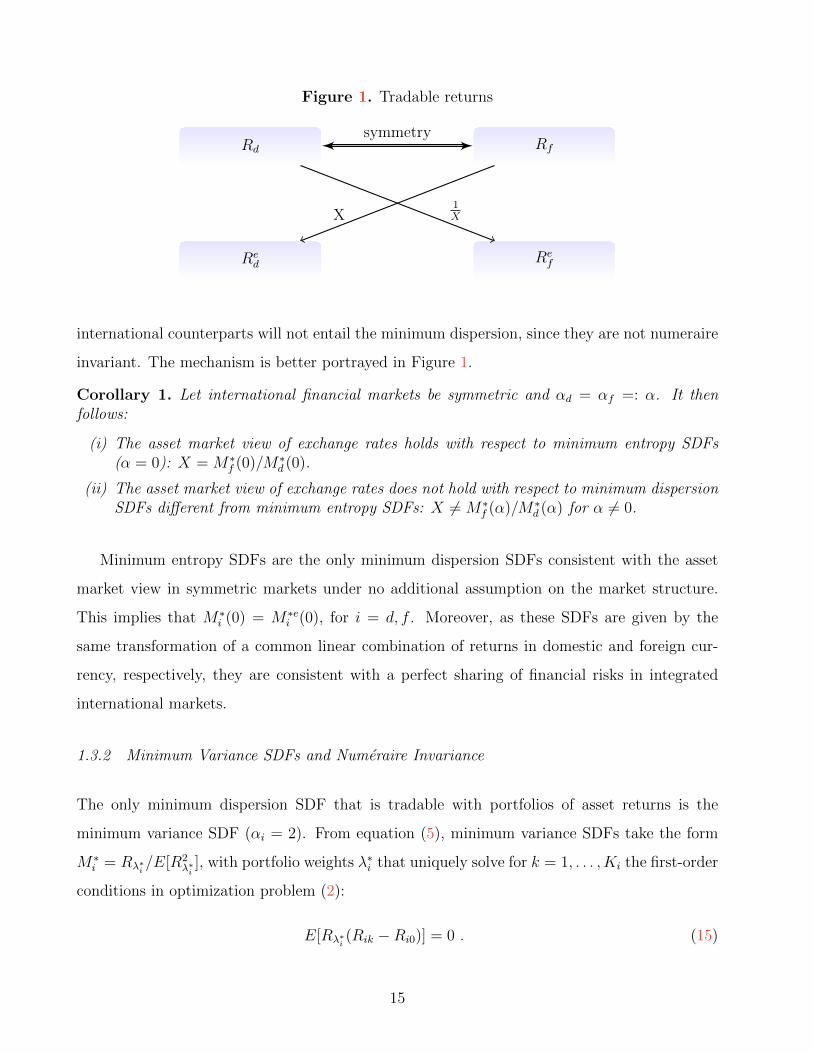
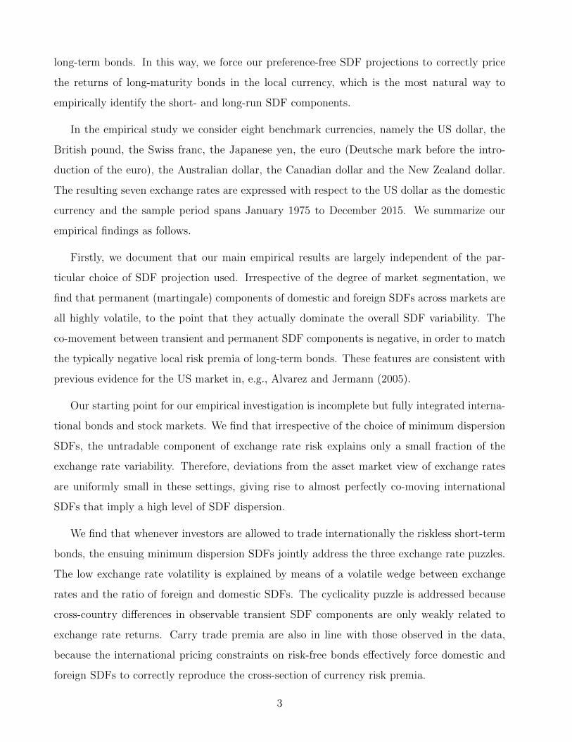
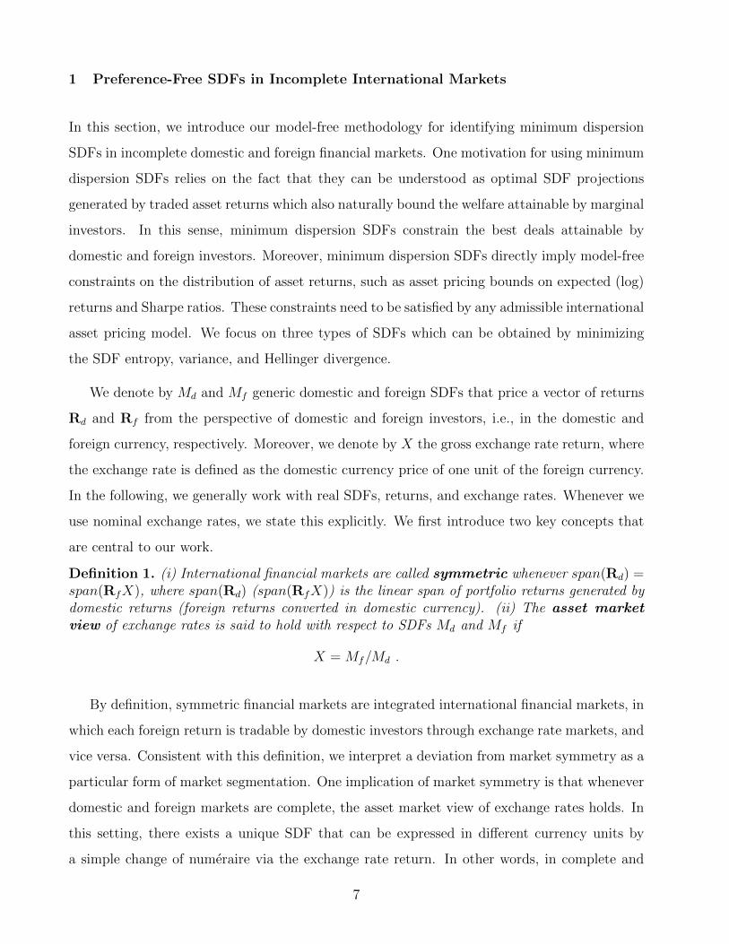
Figure 1. Tradable returns
Rd Rf
Red Re
f
X1X
symmetry
international counterparts will not entail the minimum dispersion, since they are not numeraire
invariant. The mechanism is better portrayed in Figure 1.
Corollary 1. Let international financial markets be symmetric and αd = αf =: α. It thenfollows:
(i) The asset market view of exchange rates holds with respect to minimum entropy SDFs(α = 0): X = M∗
f (0)/M∗d (0).
(ii) The asset market view of exchange rates does not hold with respect to minimum dispersionSDFs different from minimum entropy SDFs: X 6= M∗
f (α)/M∗d (α) for α 6= 0.
Minimum entropy SDFs are the only minimum dispersion SDFs consistent with the asset
market view in symmetric markets under no additional assumption on the market structure.
This implies that M∗i (0) = M∗e
i (0), for i = d, f . Moreover, as these SDFs are given by the
same transformation of a common linear combination of returns in domestic and foreign cur-
rency, respectively, they are consistent with a perfect sharing of financial risks in integrated
international markets.
1.3.2 Minimum Variance SDFs and Numeraire Invariance
The only minimum dispersion SDF that is tradable with portfolios of asset returns is the
minimum variance SDF (αi = 2). From equation (5), minimum variance SDFs take the form
M∗i = Rλ∗i
/E[R2λ∗i
], with portfolio weights λ∗i that uniquely solve for k = 1, . . . , Ki the first-order
conditions in optimization problem (2):
E[Rλ∗i(Rik −Ri0)] = 0 . (15)
15
It is an immediate consequence of these first-order conditions that minimum variance SDFs are
in general not numeraire invariant. Indeed, if M∗f (2) = Rλ∗f
/E[R2λ∗f
] is the foreign minimum
variance SDF, then M∗ed (2) := M∗
f (2)(1/X) cannot be written in general as a linear combination
of returns in vector Red. Therefore, it is not in general a minimum variance SDF for Re
d.
Symmetric arguments show that M∗ef (2) := M∗
d (2)X is not in general the minimum variance
SDF for Ref .
1.4 Minimum Dispersion SDFs and Untradable Exchange Rate Risks
One implication of the previous findings is that minimum variance SDFs are not in general
consistent with the asset market view of exchange rates. This implies that in general, M∗d (2) 6=
M∗ed (2) and M∗
f (2) 6= M∗ef (2). The origins of this violation are further understood by exploiting
the numeraire invariance of minimum entropy SDFs in Proposition 2.
Corollary 2. (i) The real exchange rate can always be decomposed as follows:
X =M∗
f (2)
M ed∗(2)·
1 + [M∗f (0)−M∗
f (2)]/M∗f (2)
1 + [M∗de(0)−M∗
de(2)]/M∗
de(2)
, (16)
=M∗
fe(2)
Md∗(2)
·1 + [M∗
fe(0)−M∗
fe(2)]/M∗
fe(2)
1 + [M∗d (0)−M∗
d (2)]/M∗d (2)
. (17)
(ii) In symmetric markets, the following exchange rate decomposition holds:
X =M∗
f (2)
M∗d (2)
·1 + [M∗
f (0)−M∗f (2)]/M∗
f (2)
1 + [M∗d (0)−M∗
d (2)]/M∗d (2)
, (18)
=Rλ∗d
(2)
Rλ∗f(2)·
1 + [Rλ∗d(0)−Rλ∗d
(2)]/Rλ∗d(2)
1 + [Rλ∗f(0)−Rλ∗f
(2)]/Rλ∗f(2)
, (19)
where Rλ∗i(αi) denotes the optimal portfolio return under dispersion parameter αi in optimiza-
tion problem (2).
Conveniently, we can compute the various decompositions in Corollary 2 from asset returns
alone. Identity (18) clarifies that a deviation from the market view with respect to minimum
variance SDFs is determined by the ratio of the relative projection errors of foreign and do-
mestic minimum entropy SDFs on the space of foreign and domestic returns. Thus, a violation
of the asset market view for minimum variance SDFs is the result of particular unspanned
exchange rate risks, which are reproduced by the component of minimum entropy SDFs that
cannot be replicated using basic asset returns. Similarly, the market view holds with respect to
16
the minimum variance SDFs whenever minimum entropy SDFs are tradable in domestic and
foreign markets, simply because in this case minimum variance and minimum entropy SDFs
are identical.
Recalling that Rλ∗i(2) and Rλ∗i
(0) are the returns of maximum Sharpe ratio and maximum
growth portfolios in market i = d, f , Corollary 2 directly characterizes exchange rates also in
terms of the tradable risk return trade-offs in international financial markets. The exchange rate
is larger when the domestic maximum Sharpe ratio return is higher than the foreign maximum
Sharpe ratio return. This effect is produced by the first quotient on the RHS of equation (19)
and can be interpreted as a tradable exchange rate effect due to the mean-variance trade-off
between domestic and foreign markets. The exchange rate is also higher when the excess return
of the domestic maximal growth return relative to the maximum Sharpe ratio return is larger
than the corresponding foreign excess return. This effect is summarized by the second quotient
on the RHS of equation (19) and directly quantifies the risk-return trade-offs between domestic
and foreign markets due to the higher moments of returns.
1.5 SDFs Similarity and the Asset Market View
An important literature in international finance attempts to quantify the amount of risk-sharing
in two countries, when the asset market view holds, based on various proxies of SDF co-
dependence. For example, Brandt, Cochrane, and Santa-Clara (2006) introduce a risk-sharing
index that is decreasing in the exchange rate variance. In a related vein, Chabi-Yo and Colac-
ito (2017) propose an index of risk-sharing based on co-entropies, which incorporates higher-
moment dependence and is decreasing in the exchange rate entropy.
In contrast to this literature, we propose a new class of SDF similarity indices, which are
independent of assumptions about the validity of the market view and can be computed from
option prices alone.
1.5.1 A SDF Similarity Index Assuming Validity of the Asset Market View
We first introduce a novel SDF similarity index for incomplete markets, which can be computed
from at-the-money currency option prices whenever the asset market view can be assumed to
17
hold. We then relax this assumption and extend our baseline index to market settings where
the market view does not hold.
Definition 2. Our index of SDF similarity is defined as follows:
S(Md,Mf ) :=E[min(Md,Mf )]
min(E[Md], E[Mf ]). (20)
By construction, S(Md,Mf ) = S(Mf ,Md), i.e. (20) is a symmetric similarity index. More-
over, 0 ≤ S(Md,Mf ) ≤ 1 and S(Md,Mf ) = 1 if and only if Md = Mf with probability one.7
Therefore, S(Md,Mf ) = 1 if and only if the exchange rate return is constant and equal to one,
while the two SDFs are more dissimilar when S(Md,Mf ) ↓ 0.
Proposition 3. If the asset market view of exchange rates holds, then
E[Md]− E[Md max(0, 1−X)]
min(E[Md], E[Mf ])= S(Md,Mf ) =
E[Mf ]− E[Mf max(0, 1− (1/X))]
min(E[Md], E[Mf ]), (21)
where max(0, 1 − X) (max(0, 1 − (1/X))) is the payoff of an at-the-money put option on the
spot exchange rate change X (1/X).
Proof: See Appendix.
It follows from Proposition 3 that whenever the asset market view holds, index (20) can
be directly computed from the price of a single domestic or foreign at-the-money put option
on the spot exchange rate return. This finding can be used empirically for various purposes.
First, it gives rise to a simple way of computing conditional similarity indices from option prices
alone. These indices can provide insight into the SDFs similarity patterns, over time and across
currencies. Second, as index S(Md,Mf ) is bounded between zero and one, empirical values of
identity (21) outside of this range may indicate a violation of the asset market view or of other
basic arbitrage-free constraints. A deviation from the asset market view may also be indicated
by a difference between the first and the second identities in equation (21). Third, conditional
on the validity of the market view, the model-free SDF similarity indices computed from options
can be taken as benchmarks for the SDF similarities of models that assume validity of the asset
market view. Whenever SDFs are specified to price real exchange rates and returns, a change
7In the trivial case where both Md and Mf are constants, the similarity index is equal to one.
18
of numeraire from real to nominal SDFs makes the model-implied similarity comparable to the
similarity computed from nominal exchange rate option prices.8
1.5.2 Relation to other SDF Similarity Indices
The normalizing constant min(E[Md], E[Mf ]) in the denominator of index (20) ensures both an
upper bound of one and the model-free index representation in Proposition 3, which is based
on the price of an at-the-money put on the spot exchange rate. Another natural approach can
directly normalize the SDFs in definition (20), which gives the similarity index:
S(Md/E[Md],Mf/E[Mf ]) := E[min(Md/E[Md],Mf/E[Mf ])] . (22)
This index preserves all key properties of index (20), but it is not computable from the prices of
options on spot exchange rates. It can be computed from the price of a single at-the-money put
on the forward exchange rate, whenever option quotes on forward exchange rates are available.9
A relevant computation issue arises for the power similarity indices introduced in Orlowski,
Sali, and Trojani (2016):
Sα(Md,Mf ) :=E[Mα
dM1−αf ]
E[Md]αE[Mf ]1−α, (23)
where α ∈ (0, 1) parameterizes the index family. This family includes for α = 1/2 the Hellinger
similarity index proposed in Bakshi, Gao, and Panayotov (2017).10 A key property of these
indices is that under the asset market view they can be in principle computed from option infor-
mation alone, whenever a continuum of out-of-the money exchange rate options with arbitrary
8Recall from Proposition 3 that this change of numeraire does not alter the optimal return structure under-lying minimum entropy SDFs.
9The following relations between the two indices hold: 0 ≤ S(Md/E[Md],Mf/E[Md]) ≤ S(Md,Mf ) ≤ 1.Moreover, under validity of the asset market view, the same arguments as in the proof of Proposition 3 yield:
E[min(Md/E[Md],Mf/E[Mf ])] = 1− 1
E[Md]E[Md max(0, 1−XE[Md]/E[Mf ])] .
10Note that:
S1/2(Md,Mf ) = E[(Md/E[Md])1/2(Mf/E[Mf ])1/2] = 1−
E[((Md/E[Md])
1/2 − (Mf/E[Mf ])1/2)2]
2.
The expectation on the RHS corresponds to Bakshi, Gao, and Panayotov (2017)’s Hellinger distance.
19
strike price K > 0 is traded, i.e., under a complete exchange rate option market.11 Unfortu-
nately, the intrinsic incompleteness of exchange rate option markets makes such a computation
of similarity index (23) very challenging. However, due to the following inequality:
S(Md,Mf )min(E[Md], E[Mf ])
E[Md]αE[Mf ]1−α≤ Sα(Md,Mf ) , (24)
we can always compute with Proposition 3 a lower bound for similarity index (23), using the
price of a single at-the-money put on the spot exchange rate.12
1.5.3 Minimal SDF Similarity Indices under a Deviation from the Asset Market View
Whenever there is a deviation from the asset market view, the SDF numeraire invariance is
not preserved and an asymmetry in the pricing properties of domestic and foreign exchange
rate options emerges. In such settings, the index S(Md,Md) cannot be computed from option
prices. In the presence of deviations from the market view, we can derive the following index
of SDF similarity:
S(Md,Mf ) := min(S(Md,Mef ), S(Mf ,M
ed)) , (25)
where M ef := MdX and M e
d := Mf (1/X). By construction, S(Md,Mf ) is a symmetric similarity
index such that 0 ≤ S(Md,Mf ) ≤ 1 and S(Md,Mf ) = S(Md,Mf ) in all cases where the
market view holds. Therefore, S(Md,Mf ) measures indeed the similarity of Md and Mf when
the market view holds. More generally, the index equals one if and only if Md = MdX and
Mf = Mf (1/X) with probability one. Therefore, S(Md,Mf ) = 1 if and only if the exchange rate
return is constant, while when Md and MdX or Mf and Mf (1/X) are more and more dissimilar,
the index shrinks. Thus, S(Md,Mf ) measures the minimal similarity among domestic and
foreign SFDs with respect to their numeraire invariant foreign and domestic SDF counterparts,
respectively.
As in Proposition 3, we can compute the similarity index (25) from two prices of a domestic
11Using standard replication formulas for nonlinear payoffs, this result follows from the identity:
Sα(Md,Mf ) =1
E[Md]αE[Mf ]1−αE[MdX
1−α] .
12The bound follows from the inequality xαy1−α ≥ min(x, y) for α ∈ (0, 1).
20
and a foreign at-the-money put option on the spot exchange rate return.
Proposition 4. Whenever the risk-free domestic and foreign returns Rf0X and Rd0(1/X) are
traded, it follows:
S(Md,Mf ) =min (E[Md]− E[Md max(0, 1−X)], E[Mf ]− E[Mf max(0, 1− (1/X))])
min(E[Md], E[Mf ]), (26)
where max(0, 1 − X) (max(0, 1 − (1/X))) is the payoff of an at-the-money put option on the
spot exchange rate change X (1/X).
Proof: See Appendix.
Proposition 4 provides a benchmark similarity index for domestic and foreign SDFs, which
is independent of the validity of the market view and can be computed from at-the-money
exchange rate option prices. This finding can be used empirically for various purposes. For
instance, whenever the prices of domestic and foreign exchange rate at-the-money options are
both observable, a comparison of indices (20) and (25) provides direct evidence on the existence
of asset market view deviations, in terms of, e.g., their dynamic properties or their cross-
sectional patterns across currencies. One can then compare these deviations to those implied
by theoretical models, under the assumption that the asset market view holds or is violated.
In cases where option quotes are available only in the domestic or the foreign currency,
Propositions 3 and 4 show that in general, i.e., also in presence of deviations from the market
view, the index computed from one of the equalities (21) is always an upper bound for the
similarity index S(Md,Mf ). As a consequence, we obtain a direct model-free diagnostics for
the model-implied similarity S(Md,Mf ) of any specification of domestic and foreign SDFs.
In our empirical analysis, we can gauge the similarity S(Md,Mf ) of minimum dispersion
SDFs under various assumptions about the degree of financial market integration, in order to
characterize market structures that can be consistent not only with the well-known exchange
rate puzzles, but also with the degree of option-implied similarity S(Md,Mf ).
1.5.4 Similarity in Benchmark Models
The index S(Md,Mf ) measures similarity, rather than SDF comovement or risk sharing. In the
following, we illustrate this using some well-known benchmark models.
21
Lognormal SDFs and Exchange Rates. Whenever (Md, X) and (Mf , 1/X) are jointly
lognormal, similarity can be directly computed from the Black and Scholes (1973)–Garman
and Kohlhagen (1983) model-implied prices of the corresponding put options:
E[Md max(0, 1−X)] = E[Md]N (−d2)− E[Mf ]N (−d1) =: BSd(σx) , (27)
E[Mf max(0, 1− (1/X))] = E[Mf ]N (d1)− E[Md]N (d2) =: BSf (σx) , (28)
where
d1 :=− log(E[Md]/E[Mf ]) + σ2
x
2
σx; d2 :=
− log(E[Md]/E[Mf ])− σ2x
2
σx, (29)
with σx the volatility of log exchange rate returns. Hence, S(Md,Mf ) is maximal (minimal)
for σx ↓ 0 (σx ↑ ∞). Given the low exchange rate volatility and the identity of physical and
implied volatilities under joint log normality, lognormal arbitrage-free settings are unlikely to
generate both a low exchange rate volatility and a low option-implied SDF similarity. Such
settings include, e.g., jointly lognormal specifications of domestic and foreign SDFs under the
asset market view.
Rare Disasters. One way to break the link between the realized and implied volatilities is to
introduce time-varying rare disasters. We borrow from Farhi and Gabaix (2016) who model an
economy with traded and nontraded goods in complete international financial markets. In this
model, a disaster may happen in the world consumption of the tradeable good with probability
pt. The exogenous SDF in units of the world numeraire, is given as follows: if no disaster
happens in t + 1, M∗t+1 = exp(−R), for a parameter R > 0 which is related to the subjective
discount rate and the expected growth rate of the tradeable good. If a disaster happens, then
M∗t+1 = exp(−R)B−γt+1, where Bt+1 models the size of world disasters and γ is the coefficient of
relative risk aversion. A key parameter in Farhi and Gabaix (2016) is a country’s resilience to
disasters, defined by:
Hit := Hi∗ + Hit := ptEDt [B−γt+1Fit+1 − 1], (30)
where Fit+1 is the future country’s recovery rate and EDt [·] denotes the expectation conditional
on a disaster state.13 Thus, a relatively safe country has a high resilience Hit, while a relatively
risky country has a low resilience. The stochastic discount factor for the nontraded good in
13By definition, Hi∗ and Hit are the constant and the time-varying components of a country’s i resilience.
22
country i depends on the time-varying resilience component Hit. It is given by:
Mit+1 = M∗t+1 ·
ωit+1
ωit· rei + φHi
+ Hit+1
rei + φHi+ Hit
, (31)
where rei is the sum of the country’s “steady state” interest rate for Hit = 0 and a constant
investment depreciation rate λ, φHiis the resilience speed of mean reversion and ωit the country’s
i export productivity. The price of a put option on the exchange rate follows from the asset
market view and the joint lognormality of red + φHd+ Hdt+1, ref + φHf
+ Hft+1 conditional on
a no disaster state.14 Therefore, the similarity index (25) is available in closed-form.
Proposition 5. In the Farhi and Gabaix (2016) model, the similarity index (25) is given by:
St(Md,Mf ) = S(Md,Mf ) =Et[Md,t+1]− Et[Md,t+1 max(0, 1−Xt+1)]
min(Et[Md,t+1], Et[Mf,t+1]), (32)
where the price of the domestic at-the-money put on the exchange rate is given by:
Et[Md,t+1 max(0, 1−Xt+1)] = (1− pt)BSd(σx)
+ptEt
[Gd,tFd,t+1 max
(0, 1− Ff,t+1Gf,t
Fd,t+1Gd,t
)], (33)
with
Gi,t = exp(gωi)rei + φHi
+ 1+Hi∗1+Hit
exp(−φHi)Hit
rei + φHi+ Hit
, (34)
and gωithe constant growth rate of country i’s productivity in no-disaster states.
Proof: See Appendix.
The first term on the RHS of equation (33) is the Black and Scholes (1973)–Garman and
Kohlhagen (1983) price of a put option, weighted by the probability of no disaster. The second
term is the put price conditional on a common disaster in domestic and foreign productivity,
weighted by the probability of a world disaster. This term reflects the price for ensuring a
large depreciation of foreign versus domestic non-traded goods, due to a larger decrease in
foreign productivity when disasters occur. This component can create a disconnect between
14See also Proposition 6 in Farhi and Gabaix (2016).
23
the minimal similarity index in Proposition 4 and the exchange rate volatility σx, which may be
useful to induce low option-implied SDF similarities together with low exchange rate volatilities.
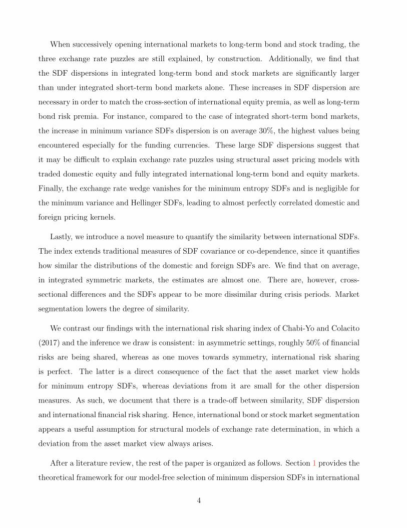
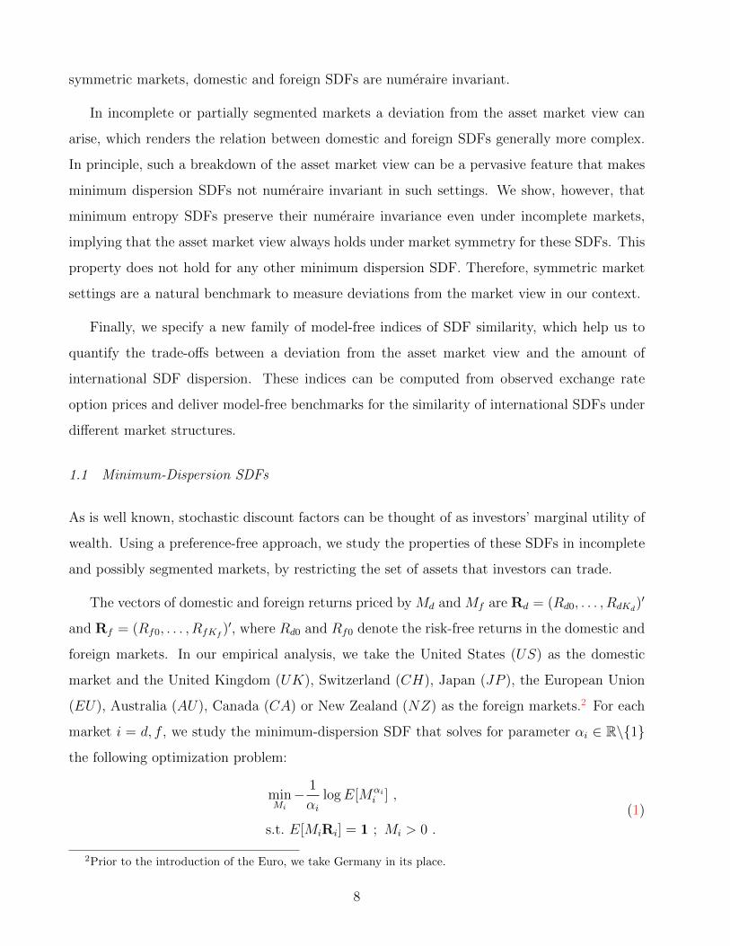
Figure 2. SDF Similarity in the Farhi and Gabaix (2016) model
0.860.08
0.88
0.04
sim
ilarit
y
0.1
0.9
x
0.92
p
0.030.12
0.14 0.02
0.080.08
0.1
0.040.1
put v
alue
0.12
x p
0.030.12
0.14
0.14 0.02
The left panel plots the similarity index given in Proposition 5 as a function of exchange rate volatility(σx) and the disaster probability (p). The right panel plots the price of the at-the-money put optionalso as a function of the exchange rate volatility and the disaster probability. Calibrated values are asin Farhi and Gabaix (2016).
We can use the calibration parameters in Farhi and Gabaix (2016) to illustrate the range
of similarity indices attainable in this model. We set gωd= gωf
= 0, σx ∈ [0.09, 0.13], pt ∈
[0.02, 0.04] and consider for simplicity the case where resilience in both countries is at its time-
invariant level, i.e., Hit = Hi∗ (i = d, f), so thatGd,t = Gf,t = 1. Conditional on a disaster event,
log recovery rates across countries are IID normally distributed, lnFit+1 ∼ IIN (−σ2Fi
2, σ2
Fi), with
calibrated standard deviation σFi= 0.16. Therefore,
Et[Fd,t+1 max (0, 1− Ff,t+1/Fd,t+1)] = N (σFi/√
2)−N (−σFi/√
2) , (35)
and the similarity index in Proposition 5 follows in closed-form. To gauge the effect of world
disasters on the similarity index, we plot in Figure 2 (left panel) the model-implied similarity
index in Proposition 5 as a function of the disaster probability (p) and the volatility of exchange
rates (σx). We notice that, on average, the similarity is around 0.88. As expected, when we
increase the volatility of exchange rates (σx) or increase the probability of rare disasters (p),
the similarity falls. This is explained by the fact that the price of the put option in the right
24
panel of Figure 2 concomitantly increases when the probability of world disasters (the volatility
of exchange rates) increases.
2 Empirical Analysis
Using our model-free minimum-dispersion SDF approach, we can now characterize and quantify
key properties of international SDFs, under different assumptions about the degree of segmen-
tation between domestic and foreign arbitrage-free financial markets. Full market integration
arises when investors have access symmetrically to all assets, both in domestic and foreign
markets: the risk-free return, the aggregate equity return and the long-term bond return. We
regard this setting as a natural starting benchmark, as equity, bond and exchange rate risk
premia are all matched by minimum dispersion SDFs under symmetric trading. In parallel,
deviations from the asset market view are either absent or small in this setting.
We seek to answer a number of key questions. First, how much dispersion is necessary
for SDFs to be able to match unconditional risk premia? Second, in order to successfully
address all three exchange rate puzzles, how are transient vs. permanent SDF components and
exchange rate wedges connected? Third, how much similarity of minimum dispersion SDFs
does a given market structure imply? Fourth, is the degree of SDF similarity compatible with
the option-implied similarity in the data? Importantly, studying these questions helps us to
identify market structures that can be consistent not only with the well-known exchange rate
puzzles, but also with the degree of option-implied SDF similarity.
Under full market integration, we estimate highly volatile and highly correlated minimum
dispersion SDFs, which successfully resolve the three exchange rate puzzles under absent or
small deviations from the asset market view. To study economies compatible with nontrivial
deviations from the market view, we consider less integrated market settings with less volatile
and less correlated SDFs, which are however still addressing the three exchange rate puzzles.
In this way, we are able to characterize the key trade-offs existing between international SDFs
dispersions and the deviations from the asset market view in incomplete markets. Finally, we
compute SDF similarity resulting from these settings and assess whether they line up with SDF
similarity recovered from option prices.
25
2.1 Data
We use monthly data between January 1975 and December 2015 from Datastream. We compute
equity returns from the corresponding MSCI country indices’ prices and risk-free rates from
one-month LIBOR rates. We follow Alvarez and Jermann (2005) and proxy transient SDF
components by the inverse of the bond return with the longest maturity available, i.e., the ten-
year (government) bonds in our case; see also Lustig, Stathopoulos, and Verdelhan (2016).15
We study eight benchmark currencies: the US dollar (USD), the British pound (GBP ), the
Swiss franc (CHF ), the Japanese yen (JPY ), the euro (EUR) (Deutsche mark (DM) before
the introduction of the euro), the Australian dollar (AUD), the Canadian dollar (CAD) and the
New Zealand dollar (NZD).16 The resulting seven exchange rates are expressed with respect
to the USD as the domestic currency.
We also use over-the-counter G10 currency options data from J. P. Morgan all quoted versus
the US dollar. Due to data limitations, our options sample starts in January 1996 and ends in
December 2013. The options used in this study are plain-vanilla European calls and puts, with
five different moneyness per currency pair. In this study, we only focus on one-month maturity
at-the-money put options.
We provide in Table 1 summary statistics for the different time-series. Panel A reports bond
market summary statistics. We find that the CHF and the JPY feature low interest rates, in line
with the intuition that they act as funding currencies in the carry trade, whereas the remaining
ones can be regarded as investment currencies. Cross-sectional differences across countries arise
with respect to unconditional long-term bond risk premia. To illustrate, (nominal) long-term
risk premia in all countries are negative, but while in Japan and Switzerland they are −0.3%
and −1.02%, respectively, in the remaining countries they range between −2.07% (EU) and
−6.06% (Australia). The fact that nominal returns on long-term bonds in local currencies are
negative has been documented also in Lustig, Stathopoulos, and Verdelhan (2016). There are
cross-sectional differences also with respect to unconditional equity premia, especially in the
15In order to study whether the ten-year bond return is a valid proxy for the (unobservable) infinite maturitybond return, a modeling assumption is needed, e.g., a family of affine term structure models on countries’yields. Lustig, Stathopoulos, and Verdelhan (2016) do not obtain significant differences between the yields of ahypothetical infinite maturity bond and a ten-year bond in such a setting.
16Throughout the paper, the sample period ranges between January 1990 to December 2015 for New Zealand,due to data availability on the long-term bonds.
26
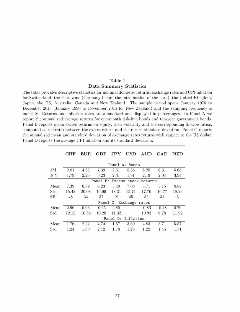
Table 1
Data Summary Statistics
The table provides descriptive statistics for nominal domestic returns, exchange rates and CPI inflationfor Switzerland, the Euro-zone (Germany before the introduction of the euro), the United Kingdom,Japan, the US, Australia, Canada and New Zealand. The sample period spans January 1975 toDecember 2015 (January 1990 to December 2015 for New Zealand) and the sampling frequency ismonthly. Returns and inflation rates are annualized and displayed in percentages. In Panel A wereport the annualized average returns for one-month risk-free bonds and ten-year government bonds.Panel B reports mean excess returns on equity, their volatility and the corresponding Sharpe ratios,computed as the ratio between the excess return and the return standard deviation. Panel C reportsthe annualized mean and standard deviation of exchange rates returns with respect to the US dollar.Panel D reports the average CPI inflation and its standard deviation.
CHF EUR GBP JPY USD AUD CAD NZD
Panel A: Bonds
1M 2.81 4.33 7.39 2.61 5.36 8.25 6.31 6.6810Y 1.79 2.26 3.23 2.31 1.91 2.19 2.04 3.94
Panel B: Excess stock returns
Mean 7.39 6.89 6.23 3.49 7.08 5.71 5.15 0.84Std 15.42 20.08 16.99 18.31 15.71 17.76 16.77 18.23SR 48 34 37 19 45 32 31 5
Panel C: Exchange rates
Mean 2.96 0.03 -0.65 2.85 -0.86 -0.48 0.76Std 12.12 10.56 10.20 11.32 10.93 6.78 11.92
Panel D: Inflation
Mean 1.76 2.22 4.74 1.57 3.69 4.83 3.71 5.57Std 1.24 1.60 2.12 1.78 1.28 1.22 1.45 1.71
27
case of Japan relative to all other countries, which exhibits a substantially lower average equity
premium of 3.49% per year. New Zealand features the lowest cross-sectional average equity
premia, but this is also an artifact of the restricted sample period. Switzerland displays the
lowest market volatility with 15.42%, while the Euro-zone has the largest one (20.08%). These
numbers imply a Sharpe ratio of 48% for Switzerland which is close to the one in the US and
a much lower Sharpe ratio for Japan, 19%.17 The unconditional average returns on exchange
rates against the US dollar also display cross-sectional variation. The highest (positive) average
return is obtained for the Swiss Franc (+2.96%), while the lowest (negative) average return
follows for the Australian dollar (−0.86%). The cross-section of unconditional exchange rate
volatilities does not exhibit significant variation, even though funding currencies, i.e., the Swiss
franc and the Japanese yen, feature a higher volatility (12.12% and 11.32%, respectively),
whereas the lowest is encountered for the Canadian dollar (6.78%). The last Panel reports
inflation statistics for the countries in our sample. The highest average inflation rates are
observed in New Zealand (5.57%) and in the UK (4.74%), while the lowest ones are those
for Japan (1.57%) and Switzerland (1.76%).18 In our empirical study, we deflate all domestic
returns and exchange rates by the corresponding domestic Consumer Price Index, in order to
obtain real returns and exchange rates.
The rich cross-sectional properties of international asset returns posit a challenge on do-
mestic and foreign SDFs, which need to be consistent with observed exchange rate regularities.
Using our model-free methodology, we quantify in the following sections the key trade-offs im-
plied by different degrees of financial market segmentation in explaining these salient features.
2.2 Unrestricted International Trading
We start our analysis with the least segmented market setting, in which investors can trade
without restrictions domestic and foreign short- and long-term bonds and stocks. The tradable
vector of returns in market i = d, f reads Ri = (Ri0, Ri1, Ri∞, Rei0, R
ei∞, R
ei1)′, where Re
d0,t+1 :=
Rf0,t+1Xt+1 (Ref0,t+1 := Rd0,t+1(1/Xt+1)) is the domestic (foreign) currency return of the foreign
17Using the whole sample period in the case of New Zealand would yield a Sharpe ratio close to the Japaneseone.
18Note that the sample includes observations associated with The Great Inflation of the 1970s and early 1980s,also known as stagflation, when markets in general exhibited large inflation rates.
28
(domestic) risk free asset, Red∞,t+1 = Rf∞,t+1Xt+1 (Re
f∞,t+1 = Rd∞,t+1(1/Xt+1)) is the domestic
(foreign) currency return of the foreign (domestic) long-term bond, and Red1,t+1 := Rf1,t+1Xt+1
(Ref1,t+1 := Rd1,t+1(1/Xt+1)) is the domestic (foreign) currency return of the foreign (domestic)
aggregate equity return. The estimated optimal portfolio return in market i = d, f is given by:
Rλ∗i ,t+1 = Ri0,t+1 + λ∗i1(Ri1,t+1 −Ri0,t+1) + λ∗i2(Ri∞,t+1 −Ri0,t+1)
+λ∗i3(Rei0,t+1 −Ri0,t+1) + λ∗i4(R
ei∞,t+1 −Ri0,t+1) + λ∗i5(R
ei1,t+1 −Ri0,t+1) . (36)
Based on these returns, the time series of estimated minimum dispersion SDFs is obtained in
closed-form from equation (5):
M∗i,t+1 =
R−1/(1−αi)
λ∗i ,t+1
Ei
[R−αi/(1−αi)
λ∗i ,t+1
] , (37)
where estimated portfolio weights in equation (36) are the unique solution of the exactly iden-
tified set of empirical moment conditions:
Ei
[R−1/(1−αi)
λ∗i(Rik −Ri0)
]= 0 , (38)
with k = 1, ..., Ki and Kd = Kf = 5 in this case. We estimate parameter vector λ∗i in
(38) using the exactly identified (generalized) method of moments. Note that as this setting
implies symmetrically traded international returns, the market view of exchange rates holds by
construction for the minimum entropy SDFs.19
2.2.1 Minimum dispersion SDFs
Since the domestic and foreign risk-free rate, bond return, and equity return are all priced
by domestic and foreign minimum dispersion SDFs, the risk premia of these returns are all
matched by construction. In particular, the currency risk premia are also exactly matched
and the forward premium anomaly is implicitly incorporated by the pricing properties of min-
19There are two additional market structures in which we can construct symmetrically traded internationalreturns, namely when investors can trade the domestic and foreign risk-free bonds only, or when they can investin both risk-free and long-term bonds domestically and abroad. As these frameworks are rather restrictive,especially the former as it does not allow for the SDF factorization into transient and permanent components,and since usually one would like to trade the equity, at least domestically, we report these results in the onlineappendix.
29
imum dispersion SDFs. We report the summary statistics of minimum dispersion SDFs under
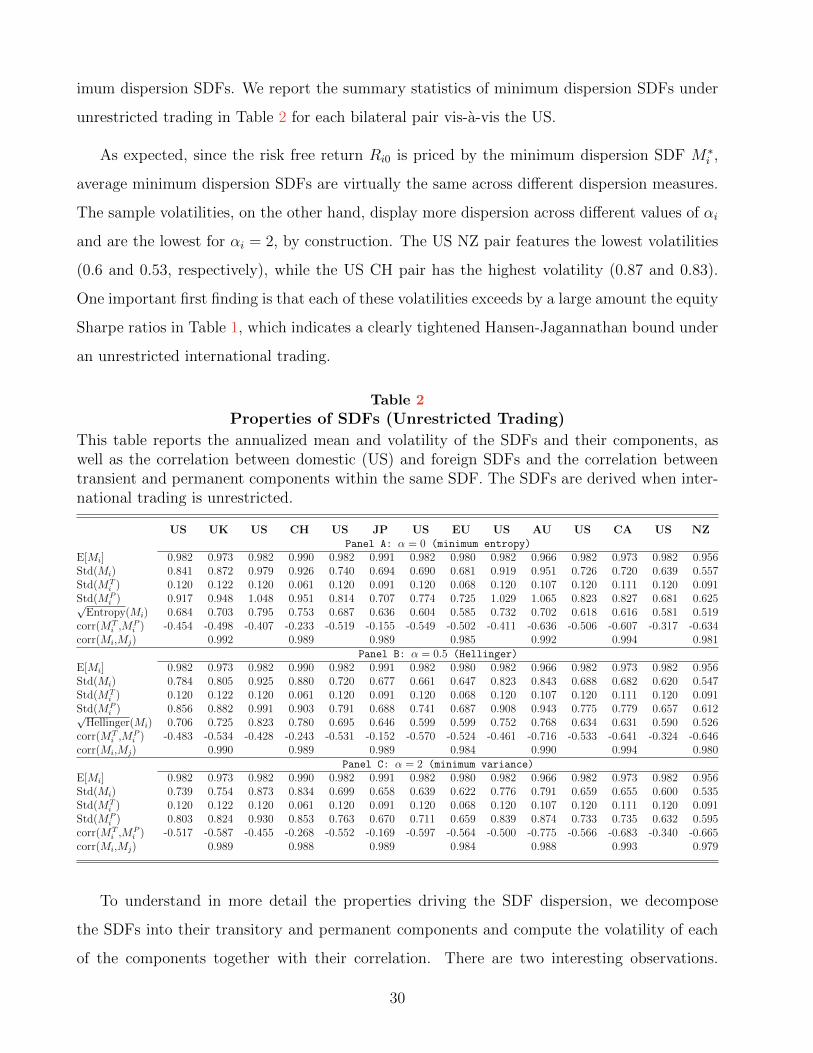
unrestricted trading in Table 2 for each bilateral pair vis-a-vis the US.
As expected, since the risk free return Ri0 is priced by the minimum dispersion SDF M∗i ,
average minimum dispersion SDFs are virtually the same across different dispersion measures.
The sample volatilities, on the other hand, display more dispersion across different values of αi
and are the lowest for αi = 2, by construction. The US NZ pair features the lowest volatilities
(0.6 and 0.53, respectively), while the US CH pair has the highest volatility (0.87 and 0.83).
One important first finding is that each of these volatilities exceeds by a large amount the equity
Sharpe ratios in Table 1, which indicates a clearly tightened Hansen-Jagannathan bound under
an unrestricted international trading.
Table 2
Properties of SDFs (Unrestricted Trading)
This table reports the annualized mean and volatility of the SDFs and their components, aswell as the correlation between domestic (US) and foreign SDFs and the correlation betweentransient and permanent components within the same SDF. The SDFs are derived when inter-national trading is unrestricted.
US UK US CH US JP US EU US AU US CA US NZPanel A: α = 0 (minimum entropy)
E[Mi] 0.982 0.973 0.982 0.990 0.982 0.991 0.982 0.980 0.982 0.966 0.982 0.973 0.982 0.956Std(Mi) 0.841 0.872 0.979 0.926 0.740 0.694 0.690 0.681 0.919 0.951 0.726 0.720 0.639 0.557Std(MT
i ) 0.120 0.122 0.120 0.061 0.120 0.091 0.120 0.068 0.120 0.107 0.120 0.111 0.120 0.091Std(MP
i ) 0.917 0.948 1.048 0.951 0.814 0.707 0.774 0.725 1.029 1.065 0.823 0.827 0.681 0.625√Entropy(Mi) 0.684 0.703 0.795 0.753 0.687 0.636 0.604 0.585 0.732 0.702 0.618 0.616 0.581 0.519
corr(MTi ,MP
i ) -0.454 -0.498 -0.407 -0.233 -0.519 -0.155 -0.549 -0.502 -0.411 -0.636 -0.506 -0.607 -0.317 -0.634corr(Mi,Mj) 0.992 0.989 0.989 0.985 0.992 0.994 0.981
Panel B: α = 0.5 (Hellinger)
E[Mi] 0.982 0.973 0.982 0.990 0.982 0.991 0.982 0.980 0.982 0.966 0.982 0.973 0.982 0.956Std(Mi) 0.784 0.805 0.925 0.880 0.720 0.677 0.661 0.647 0.823 0.843 0.688 0.682 0.620 0.547Std(MT
i ) 0.120 0.122 0.120 0.061 0.120 0.091 0.120 0.068 0.120 0.107 0.120 0.111 0.120 0.091Std(MP
i ) 0.856 0.882 0.991 0.903 0.791 0.688 0.741 0.687 0.908 0.943 0.775 0.779 0.657 0.612√Hellinger(Mi) 0.706 0.725 0.823 0.780 0.695 0.646 0.599 0.599 0.752 0.768 0.634 0.631 0.590 0.526
corr(MTi ,MP
i ) -0.483 -0.534 -0.428 -0.243 -0.531 -0.152 -0.570 -0.524 -0.461 -0.716 -0.533 -0.641 -0.324 -0.646corr(Mi,Mj) 0.990 0.989 0.989 0.984 0.990 0.994 0.980
Panel C: α = 2 (minimum variance)
E[Mi] 0.982 0.973 0.982 0.990 0.982 0.991 0.982 0.980 0.982 0.966 0.982 0.973 0.982 0.956Std(Mi) 0.739 0.754 0.873 0.834 0.699 0.658 0.639 0.622 0.776 0.791 0.659 0.655 0.600 0.535Std(MT
i ) 0.120 0.122 0.120 0.061 0.120 0.091 0.120 0.068 0.120 0.107 0.120 0.111 0.120 0.091Std(MP
i ) 0.803 0.824 0.930 0.853 0.763 0.670 0.711 0.659 0.839 0.874 0.733 0.735 0.632 0.595corr(MT
i ,MPi ) -0.517 -0.587 -0.455 -0.268 -0.552 -0.169 -0.597 -0.564 -0.500 -0.775 -0.566 -0.683 -0.340 -0.665
corr(Mi,Mj) 0.989 0.988 0.989 0.984 0.988 0.993 0.979
To understand in more detail the properties driving the SDF dispersion, we decompose
the SDFs into their transitory and permanent components and compute the volatility of each
of the components together with their correlation. There are two interesting observations.
30
First, almost all of the SDF volatility is generated by the permanent component, regardless of
the country or dispersion measure considered. This is in line with US evidence in Alvarez and
Jermann (2005) who find that to be consistent with the low returns on long-term bonds relative
to equity, the permanent component of SDFs have to be very large. Second, the correlation
between US and foreign SDFs are virtually perfect, which is a first broad indication of a high
SDF similarity. For example, the lowest correlation between SDFs is for the US and NZ pair
which is 97.9%.
2.2.2 Exchange Rate Volatilities and Wedges
The large SDF co-movement under fully integrated markets is directly related to the low ex-
change rate volatility puzzle in Brandt, Cochrane, and Santa-Clara (2006), who show that when
the asset market view holds international SDFs need to be almost perfectly correlated to match
the low exchange rate volatility.
In our incomplete market setting, the large SDF correlation is related to the properties of
the permanent SDF components. This seemingly perfect co-movement can be understood by
rearranging terms in equation (11), to get the following identity:
Xt+1Rf∞,t+1
Rd∞,t+1
=MP
f,t+1
MPd,t+1
eηt+1 . (39)
The low variability of the LHS of identity (39) in the data (low exchange rate volatility puzzle)
can be explained either by a low variability of both the ratio of permanent SDF components and
the wedge, by a strong negative co-movement between the ratio of permanent SDF components
and the wedge, or by a combination of these effects. A direct implication of these properties is
that under the market view (i.e., ηt+1 = 0) permanent components need to be almost perfectly
positively related. In contrast, in a setting where the market view is not satisfied, a trade-off
between the co-movement of the permanent SDF components and the long-run cyclicality of
exchange rate wedges emerges.
It follows that the high SDF dispersions in Table 2 can be empirically consistent with
identity (39) only in presence of a sufficiently large wedge dispersion or when permanent SDF
components are strongly positively correlated. To study this trade-off in detail, we compute
31
wedge summary statistics consistent with identity (39):
Xt+1 exp(−ηt+1) =R
1/(1−αd)
λ∗d,t+1R−1/(1−αf )
λ∗f ,t+1
Ed
[R−αd/(1−αd)
λ∗d,t+1
]−1Ef
[R−αf/(1−αf )
λ∗f ,t+1
] . (40)
where the optimal returns are given in equation (36). Summary statistics of the wedge in the
setting with unrestricted trading are reported in Table 3, where we focus on minimum variance
and minimum Hellinger SDFs alone, because the wedge resulting from minimum entropy SDFs
vanishes by construction (see Corollary 1). Consistent with the above intuition, we obtain a
Table 3
Wedge Summary Statistics (Unrestricted Trading)
This table reports the annualized mean, standard deviation, skewness and kurtosis of thewedge η, for α ∈ {0.5, 2}. The domestic currency is the US dollar. The wedge is ηt+1 =
log(Xt+1Md,t+1
Mf,t+1
). The minimum dispersion SDFs account for the fact that domestic investors
can trade any foreign asset.
α = 0.5 α = 2E[η] Std(η) Sk(η) K(η) E[η] Std(η) Sk(η) K(η)
UK 0.000 0.022 -0.395 6.336 -0.007 0.059 -0.259 11.62CH -0.001 0.026 -1.277 8.426 -0.019 0.120 -6.146 68.40JP 0.000 0.023 -1.286 7.608 -0.009 0.083 -4.483 36.18EU 0.000 0.021 -0.065 5.814 0.000 0.064 -1.130 11.47AU 0.000 0.019 0.424 8.003 0.005 0.075 2.110 24.82CA 0.000 0.013 -0.488 6.080 -0.001 0.034 -0.538 5.772NZ -0.001 0.023 -2.695 17.23 -0.031 0.216 -15.61 268.3
very small wedge dispersion in all cases. The smallest wedges arise for the minimum Hellinger
divergence SDFs, which are the most related to minimum entropy SDFs. We also notice that
the wedge implied by minimum variance SDFs can only contribute a negligible fraction to the
overall exchange rate volatility given (39).20
As we ruled out that wedges have any strong bearing on the volatility of exchange rates,
we focus next on the co-movement between martingale components. Table 4 reports the av-
erage correlations across different exchange rate pairs, showing that there is almost perfect
20Lustig and Verdelhan (2016) show that in order to match the low exchange rate volatility puzzle usingequation (10), the wedge needs to covary positively (negatively) with the domestic (foreign) SDF, i.e., it needsto be pro-cyclical. Given the very low wedge dispersion, the cyclicality properties are not particularly insightfulin the fully integrated market setting and we do not report them here to save space.
32
co-movement across all currency pairs. Therefore, we anticipate that in fully integrated mar-
kets, minimum dispersion SDFs are very similar and highly disperse, mainly due to their very
similar and highly disperse permanent components.
Table 4
Correlation of Permanent SDF Components Across Exchange Rate ParitiesThis table reports the correlation between permanent components of domestic and foreign SDFs. Thedomestic SDF is the US one, whereas the foreign SDFs are those for the UK, CH, JP, EU, AU,CA and NZ. Standard errors are computed using a circular block bootstrap of size 10 with 10, 000simulations and reported in square brackets. Labels ∗∗ and ∗∗∗ denote significance at the 5% and 1%level, respectively.
UK CH JP EU AU CA NZ
corr(MPd ,MP
f )
α = 0 0.972∗∗∗ 0.984∗∗∗ 0.981∗∗∗ 0.978∗∗∗ 0.987∗∗∗ 0.976∗∗∗ 0.968∗∗∗
[0.019] [0.007] [0.004] [0.007] [0.006] [0.005] [0.006]α = 0.5 0.969∗∗∗ 0.984∗∗∗ 0.980∗∗∗ 0.976∗∗∗ 0.984∗∗∗ 0.975∗∗∗ 0.968∗∗∗
[0.013] [0.004] [0.004] [0.006] [0.005] [0.005] [0.005]α = 2 0.968∗∗∗ 0.982∗∗∗ 0.977∗∗∗ 0.974∗∗∗ 0.980∗∗∗ 0.973∗∗∗ 0.965∗∗∗
[0.009] [0.003] [0.004] [0.006] [0.005] [0.004] [0.005]
2.2.3 Backus-Smith (1993) Puzzle
As the setting with fully integrated markets can incorporate both the forward premium anomaly
and the low exchange rate volatility, we focus in this section on the exchange rate cyclicality
by means of Backus and Smith (1993)-type regressions:
mf,t+1 −md,t+1 = δ + βxt+1 + ut+1,
mUf,t+1 −mU
d,t+1 = δU + βUxt+1 + uUt+1,
for U = T, P , where we regress both the log difference between foreign and domestic SDFs and
their transient and permanent components on the log exchange rate return xt+1.
When the asset market view holds, the population point estimate from these regressions
based on the overall SDFs is exactly one. This case emerges for the minimum entropy SDFs
under fully integrated markets. More generally, when risk-free returns are traded internation-
ally, Lustig and Verdelhan (2016) show that the same finding holds also under a deviation from
the market view. Therefore, we expect similar findings also for mimimum variance and mini-
mum Hellinger divergence SDFs. Finally, since the SDF variability in Table 2 is dominated by
33
the permanent component, we expect similar implications for regressions using the persistent
SDF components.
Table 5
Backus-Smith (1993)-Type Regressions (Unrestricted Trading)
This table reports the point estimates of a linear regression of the log difference between foreign and domesticSDFs on the log real exchange rate return: mf,t+1 −md,t+1 = δ+ βxt+1 + ut+1, where small-cap letters denotequantities in logs. We additionally report point estimates of a linear regression of the log difference of eachcomponent of the SDF on the log change in the real exchange rate: mU
f,t+1 −mUd,t+1 = δU + βUxt+1 + uUt+1,
where U = P, T for permanent and transitory components, respectively. Standard errors are reported in squarebrackets. Label ∗∗∗ highlights significance at the 1% level.
Panel A: US/UK Panel B: US/CHα = 0 α = 0.5 α = 2 α = 0 α = 0.5 α = 2
β 1.000∗∗∗ 1.060∗∗∗ 1.022∗∗∗ 1.000∗∗∗ 1.079∗∗∗ 1.233∗∗∗
[0.000] [0.009] [0.0261] [0.000] [0.009] [0.043]βP 1.085∗∗∗ 1.145∗∗∗ 1.065∗∗∗ 0.951∗∗∗ 1.030∗∗∗ 1.183∗∗∗
[0.068] [0.067] [0.0742] [0.044] [0.045] [0.064]βT -0.084 -0.084 -0.084 0.049 0.049 0.049
[0.068] [0.068] [0.068] [0.044] [0.044] [0.044]Panel C: US/JP Panel D: US/EU
α = 0 α = 0.5 α = 2 α = 0 α = 0.5 α = 2β 1.000∗∗∗ 1.056∗∗∗ 1.107∗∗∗ 1.000∗∗∗ 1.050∗∗∗ 1.055∗∗∗
[0.000] [0.009] [0.033] [0.000] [0.008] [0.027]βP 1.083∗∗∗ 1.139∗∗∗ 1.189∗∗∗ 0.956∗∗∗ 1.006∗∗∗ 1.011∗∗∗
[0.053] [0.053] [0.065] [0.046] [0.046] [0.056]βT -0.083 -0.083 -0.083 0.044 0.044 0.044
[0.053] [0.053] [0.053] [0.046] [0.046] [0.046]Panel E: US/AU Panel F: US/CA
α = 0 α = 0.5 α = 2 α = 0 α = 0.5 α = 2β 1.000∗∗∗ 1.042∗∗∗ 1.117∗∗∗ 1.000∗∗∗ 1.044∗∗∗ 1.031∗∗∗
[0.000] [0.007] [0.029] [0.000] [0.008] [0.022]βP 1.005∗∗∗ 1.047∗∗∗ 1.122∗∗∗ 1.027∗∗∗ 1.072∗∗∗ 1.059∗∗∗
[0.049] [0.049] [0.059] [0.089] [0.090] [0.093]βT -0.005 -0.005 -0.005 -0.028 -0.028 -0.028
[0.049] [0.049] [0.049] [0.089] [0.089] [0.089]Panel G: US/NZ
α = 0 α = 0.5 α = 2β 1.000∗∗∗ 1.055∗∗∗ 1.409∗∗∗
[0.000] [0.009] [0.095]βP 1.006∗∗∗ 1.061∗∗∗ 1.415∗∗∗
[0.038] [0.038] [0.098]βT -0.006 -0.006 -0.006
[0.037] [0.037] [0.037]
34
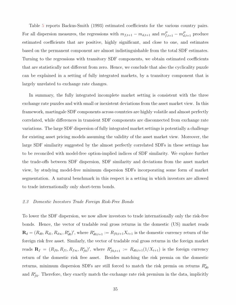
Table 5 reports Backus-Smith (1993) estimated coefficients for the various country pairs.
For all dispersion measures, the regressions with mf,t+1 −md,t+1 and mPf,t+1 −mP
d,t+1 produce
estimated coefficients that are positive, highly significant, and close to one, and estimates
based on the permanent component are almost indistinguishable from the total SDF estimates.
Turning to the regressions with transitory SDF components, we obtain estimated coefficients
that are statistically not different from zero. Hence, we conclude that also the cyclicality puzzle
can be explained in a setting of fully integrated markets, by a transitory component that is
largely unrelated to exchange rate changes.
In summary, the fully integrated incomplete market setting is consistent with the three
exchange rate puzzles and with small or inexistent deviations from the asset market view. In this
framework, martingale SDF components across countries are highly volatile and almost perfectly
correlated, while differences in transient SDF components are disconnected from exchange rate
variations. The large SDF dispersion of fully integrated market settings is potentially a challenge
for existing asset pricing models assuming the validity of the asset market view. Moreover, the
large SDF similarity suggested by the almost perfectly correlated SDFs in these settings has
to be reconciled with model-free option-implied indices of SDF similarity. We explore further
the trade-offs between SDF dispersion, SDF similarity and deviations from the asset market
view, by studying model-free minimum dispersion SDFs incorporating some form of market
segmentation. A natural benchmark in this respect is a setting in which investors are allowed
to trade internationally only short-term bonds.
2.3 Domestic Investors Trade Foreign Risk-Free Bonds
To lower the SDF dispersion, we now allow investors to trade internationally only the risk-free
bonds. Hence, the vector of tradable real gross returns in the domestic (US) market reads
Rd = (Rd0, Rd1, Rd∞, Red0)′, where Re
d0,t+1 := Rf0,t+1Xt+1 is the domestic currency return of the
foreign risk free asset. Similarly, the vector of tradable real gross returns in the foreign market
reads Rf = (Rf0, Rf1, Rf∞, Ref0)′, where Re
f0,t+1 := Rd0,t+1(1/Xt+1) is the foreign currency
return of the domestic risk free asset. Besides matching the risk premia on the domestic
returns, minimum dispersion SDFs are still forced to match the risk premia on returns Red0
and Ref0. Therefore, they exactly match the exchange rate risk premium in the data, implicitly
35
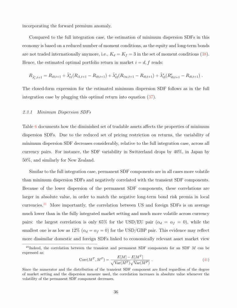
incorporating the forward premium anomaly.
Compared to the full integration case, the estimation of minimum dispersion SDFs in this
economy is based on a reduced number of moment conditions, as the equity and long-term bonds
are not traded internationally anymore, i.e., Kd = Kf = 3 in the set of moment conditions (38).
Hence, the estimated optimal portfolio return in market i = d, f reads:
Rλ∗i ,t+1 = Ri0,t+1 + λ∗i1(Ri1,t+1 −Ri0,t+1) + λ∗i2(Ri∞,t+1 −Ri0,t+1) + λ∗i3(Rei0,t+1 −Ri0,t+1) .
The closed-form expression for the estimated minimum dispersion SDF follows as in the full
integration case by plugging this optimal return into equation (37).
2.3.1 Minimum Dispersion SDFs
Table 6 documents how the diminished set of tradable assets affects the properties of minimum
dispersion SDFs. Due to the reduced set of pricing restriction on returns, the variability of
minimum dispersion SDF decreases considerably, relative to the full integration case, across all
currency pairs. For instance, the SDF variability in Switzerland drops by 40%, in Japan by
50%, and similarly for New Zealand.
Similar to the full integration case, permanent SDF components are in all cases more volatile
than minimum dispersion SDFs and negatively correlated with the transient SDF components.
Because of the lower dispersion of the permanent SDF components, these correlations are
larger in absolute value, in order to match the negative long-term bond risk premia in local
currencies.21 More importantly, the correlation between US and foreign SDFs is on average
much lower than in the fully integrated market setting and much more volatile across currency
pairs: the largest correlation is only 65% for the USD/EU pair (αd = αf = 0), while the
smallest one is as low as 12% (αd = αf = 0) for the USD/GBP pair. This evidence may reflect
more dissimilar domestic and foreign SDFs linked to economically relevant asset market view
21Indeed, the correlation between the transient and permanent SDF components for an SDF M can beexpressed as:
Corr(MT ,MP ) =E[M ]− E[MT ]√
Var(MT )√
Var(MP ). (41)
Since the numerator and the distribution of the transient SDF component are fixed regardless of the degreeof market setting and the dispersion measure used, the correlation increases in absolute value whenever thevolatility of the permanent SDF component decreases.
36
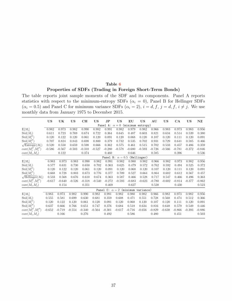
Table 6
Properties of SDFs (Trading in Foreign Short-Term Bonds)
The table reports joint sample moments of the SDF and its components. Panel A reportsstatistics with respect to the minimum-entropy SDFs (αi = 0), Panel B for Hellinger SDFs(αi = 0.5) and Panel C for minimum variance SDFs (αi = 2), i = d, f , j = d, f , i 6= j. We usemonthly data from January 1975 to December 2015.
US UK US CH US JP US EU US AU US CA US NZPanel A: α = 0 (minimum entropy)
E[Mi] 0.982 0.973 0.982 0.990 0.982 0.991 0.982 0.979 0.982 0.966 0.983 0.973 0.983 0.956Std(Mi) 0.611 0.723 0.769 0.674 0.722 0.364 0.645 0.487 0.603 0.821 0.634 0.514 0.539 0.380Std(MT
i ) 0.120 0.122 0.120 0.061 0.120 0.091 0.120 0.068 0.120 0.107 0.120 0.111 0.120 0.091Std(MP
i ) 0.707 0.824 0.843 0.698 0.800 0.379 0.732 0.535 0.702 0.931 0.729 0.641 0.585 0.466√Entropy(Mi) 0.520 0.550 0.659 0.598 0.666 0.362 0.575 0.461 0.515 0.702 0.533 0.457 0.486 0.359
corr(MTi ,MP
i ) -0.586 -0.567 -0.503 -0.310 -0.527 -0.280 -0.578 -0.680 -0.593 -0.726 -0.566 -0.781 -0.372 -0.846corr(Mi,Mj) 0.122 0.374 0.460 0.646 0.585 0.396 0.536
Panel B: α = 0.5 (Hellinger)
E[Mi] 0.983 0.973 0.983 0.990 0.982 0.991 0.982 0.980 0.982 0.966 0.982 0.973 0.982 0.956Std(Mi) 0.577 0.631 0.730 0.650 0.702 0.363 0.625 0.479 0.572 0.762 0.592 0.494 0.525 0.372Std(MT
i ) 0.120 0.122 0.120 0.061 0.120 0.091 0.120 0.068 0.120 0.107 0.120 0.111 0.120 0.091Std(MP
i ) 0.668 0.728 0.803 0.673 0.776 0.377 0.709 0.527 0.664 0.864 0.682 0.612 0.567 0.457√Hellinger(Mi) 0.533 0.568 0.676 0.610 0.674 0.363 0.587 0.466 0.528 0.717 0.547 0.466 0.496 0.363
corr(MTi ,MP
i ) -0.617 -0.640 -0.526 -0.318 -0.540 -0.272 -0.593 -0.683 -0.623 -0.780 -0.602 -0.814 -0.377 -0.862corr(Mi,Mj) 0.154 0.351 0.469 0.627 0.538 0.430 0.523
Panel C: α = 2 (minimum variance)
E[Mi] 0.983 0.973 0.982 0.990 0.982 0.991 0.982 0.980 0.982 0.966 0.982 0.973 0.982 0.956Std(Mi) 0.555 0.581 0.699 0.630 0.681 0.359 0.608 0.471 0.551 0.728 0.568 0.474 0.512 0.366Std(MT
i ) 0.120 0.122 0.120 0.061 0.120 0.091 0.120 0.068 0.120 0.107 0.120 0.111 0.120 0.091Std(MP
i ) 0.637 0.666 0.766 0.651 0.747 0.376 0.684 0.518 0.634 0.816 0.648 0.579 0.549 0.446corr(MT
i ,MPi ) -0.652 -0.719 -0.554 -0.340 -0.564 -0.301 -0.617 -0.716 -0.656 -0.829 -0.638 -0.866 -0.393 -0.886
corr(Mi,Mj) 0.166 0.276 0.492 0.586 0.480 0.451 0.503
37
deviations across currencies.
2.3.2 Exchange Rate Volatility and Wedges
Intuitively, the presence of more pronunced asset market view deviations in the setting with
internationally traded risk-free bonds alone suggests a larger exchange rate wedge variability.
Table 7
Wedge Summary Statistics (Trading in Foreign Short-Term Bonds)
The table reports sample mean, standard deviation, skewness and kurtosis of the wedge in equation(10) (ηt+1 = log((Md,t+1Xt+1)/Mf,t+1)), for dispersion measures α = 0, 0.5, 2. The optimal derivedSDFs account for the fact that domestic investors can trade the short-term foreign risk-free bond.
α = 0 α = 0.5 α = 2E[η] Std(η) Sk(η) K(η) E[η] Std(η) Sk(η) K(η) E[η] Std(η) Sk(η) K(η)
UK 0.003 0.636 -0.646 13.55 0.005 0.665 -0.207 6.847 0.042 0.814 1.074 9.239CH -0.006 0.682 -0.367 6.270 -0.007 0.713 -0.174 4.647 -0.021 0.826 -0.019 3.724JP -0.123 0.545 1.446 8.938 -0.124 0.554 1.053 6.713 -0.149 0.612 -0.259 5.417EU -0.048 0.439 0.265 4.026 -0.048 0.455 0.058 3.629 -0.059 0.517 -0.554 5.011AU 0.104 0.581 -0.181 5.573 0.106 0.614 0.050 4.898 0.129 0.716 1.051 6.714CA -0.036 0.490 0.148 9.963 -0.036 0.507 0.093 5.655 -0.040 0.561 0.305 5.082NZ -0.020 0.413 0.362 4.556 -0.021 0.419 0.265 4.045 -0.029 0.442 0.178 3.834
Table 7 reports summary wedge statistics that support this intuition. Overall, we obtain
wedges that are similarly volatile as minimum dispersion SDFs, with higher moments that
reflect the non-normality of exchange rate returns in a way that depends on the choice of
minimum dispersion SDFs in incomplete markets.22
Because of these deviations from the asset market view, the wedge displays now a non-trivial
cyclicality with respect to the minimum dispersion SDFs. The wedge cyclicality properties are
summarized in Table 8, which reports the average correlations between wedges and minimum
dispersion SDFs. We obtain a pro-cyclicality that is explained by a pronounced positive (neg-
ative) wedge correlation with the permanent components of domestic (foreign) SDFs. The
co-movement with the transient component is instead typically weaker and of opposite sign.
22Especially for UK, CH and AU markets, we obtain wedges with fatter tails and opposite signs for skewnessunder parameter choices αi = 2 and αi = 0, 0.5, respectively. This last feature is a consequence of the factthat the minimum variance SDF does not capture the higher moment features linked to extreme exchange ratemovements as strongly as the other two minimum dispersion SDFs.
38

Table 8
Correlation Between Wedge and SDFs (Trading in Foreign Short-Term Bonds)
This table reports the correlation between the wedge η, the (log) domestic and foreign minimum
entropy SDFs (α = 0), as well as the log permanent and transient components of minimum entropy
SDFs. Log SDFs are denoted by mi := logMi and log SDF components by mUi := logMU
i (i = d, f
and U = T, P ). Standard errors (SE) are computed using a circular block bootstrap of size 10 with
10000 simulations and reported in square brackets. ∗∗∗ denotes significance at the 1% level.
corr(η,mi) SE corr(η,mPi ) SE corr(η,mT
i ) SE
US 0.658∗∗∗ [0.039] 0.651∗∗∗ [0.039] -0.356∗∗∗ [0.049]UK -0.617∗∗∗ [0.052] -0.602∗∗∗ [0.057] 0.338∗∗∗ [0.053]
US 0.541∗∗∗ [0.026] 0.569∗∗∗ [0.029] -0.431∗∗∗ [0.038]CH -0.594∗∗∗ [0.051] -0.585∗∗∗ [0.053] 0.077 [0.054]
US 0.728∗∗∗ [0.039] 0.759∗∗∗ [0.042] -0.532∗∗∗ [0.058]JP -0.201∗∗∗ [0.054] -0.200∗∗∗ [0.056] -0.029 [0.061]
US 0.552∗∗∗ [0.047] 0.546∗∗∗ [0.050] -0.273∗∗∗ [0.058]EU -0.296∗∗∗ [0.084] -0.324∗∗∗ [0.909] 0.402∗∗∗ [0.052]
US 0.257∗∗∗ [0.062] 0.204∗∗∗ [0.065] 0.087 [0.057]AU -0.685∗∗∗ [0.049] -0.714∗∗∗ [0.044] 0.756∗∗∗ [0.030]
US 0.606∗∗∗ [0.077] 0.605∗∗∗ [0.076] -0.342∗∗∗ [0.055]CA -0.426∗∗∗ [0.120] -0.470∗∗∗ [0.111] 0.565∗∗∗ [0.069]
US 0.523∗∗∗ [0.031] 0.441∗∗∗ [0.040] 0.278∗∗∗ [0.039]NZ -0.465∗∗∗ [0.075] -0.508∗∗∗ [0.071] 0.606∗∗∗ [0.057]
In summary, the economy with internationally traded risk-free bonds alone can incorporate
both the forward premium anomaly and the low exchange rate volatility by means of a volatile
exchange rate wedge.
2.3.3 Backus-Smith (1993) Puzzle
Consistently with the evidence in the last section, SDFs incorporating martingale components
can support the low co-movement of cross-sectional differences in consumption growth and
exchange rate returns, i.e., the exchange rate cyclicality properties. Table 9 quantifies these
relations by reporting the point estimates of Backus-Smith (1993)-type regressions of log differ-
ences in minimum dispersion SDFs and martingale SDF components on real log exchange rate
39
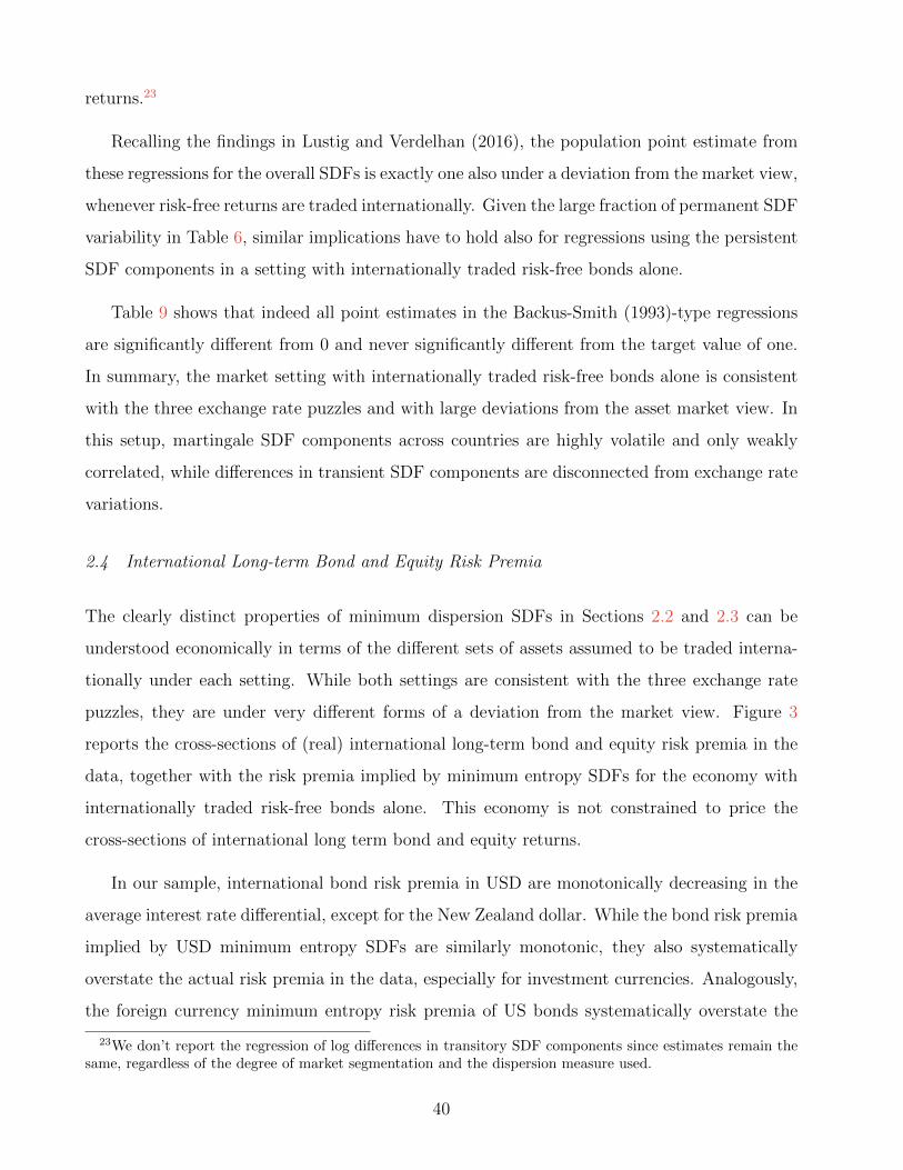
returns.23
Recalling the findings in Lustig and Verdelhan (2016), the population point estimate from
these regressions for the overall SDFs is exactly one also under a deviation from the market view,
whenever risk-free returns are traded internationally. Given the large fraction of permanent SDF
variability in Table 6, similar implications have to hold also for regressions using the persistent
SDF components in a setting with internationally traded risk-free bonds alone.
Table 9 shows that indeed all point estimates in the Backus-Smith (1993)-type regressions
are significantly different from 0 and never significantly different from the target value of one.
In summary, the market setting with internationally traded risk-free bonds alone is consistent
with the three exchange rate puzzles and with large deviations from the asset market view. In
this setup, martingale SDF components across countries are highly volatile and only weakly
correlated, while differences in transient SDF components are disconnected from exchange rate
variations.
2.4 International Long-term Bond and Equity Risk Premia
The clearly distinct properties of minimum dispersion SDFs in Sections 2.2 and 2.3 can be
understood economically in terms of the different sets of assets assumed to be traded interna-
tionally under each setting. While both settings are consistent with the three exchange rate
puzzles, they are under very different forms of a deviation from the market view. Figure 3
reports the cross-sections of (real) international long-term bond and equity risk premia in the
data, together with the risk premia implied by minimum entropy SDFs for the economy with
internationally traded risk-free bonds alone. This economy is not constrained to price the
cross-sections of international long term bond and equity returns.
In our sample, international bond risk premia in USD are monotonically decreasing in the
average interest rate differential, except for the New Zealand dollar. While the bond risk premia
implied by USD minimum entropy SDFs are similarly monotonic, they also systematically
overstate the actual risk premia in the data, especially for investment currencies. Analogously,
the foreign currency minimum entropy risk premia of US bonds systematically overstate the
23We don’t report the regression of log differences in transitory SDF components since estimates remain thesame, regardless of the degree of market segmentation and the dispersion measure used.
40
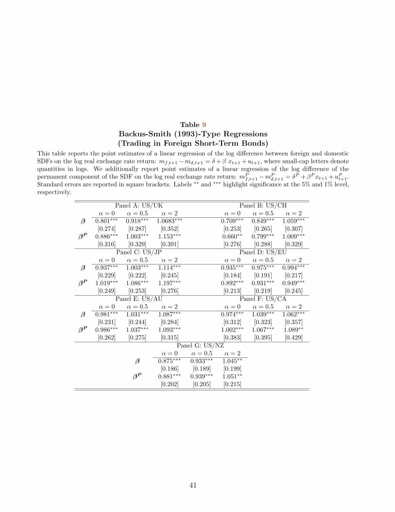
Table 9
Backus-Smith (1993)-Type Regressions(Trading in Foreign Short-Term Bonds)
This table reports the point estimates of a linear regression of the log difference between foreign and domesticSDFs on the log real exchange rate return: mf,t+1−md,t+1 = δ+β xt+1 +ut+1, where small-cap letters denotequantities in logs. We additionally report point estimates of a linear regression of the log difference of thepermanent component of the SDF on the log real exchange rate return: mP
f,t+1−mPd,t+1 = δP +βPxt+1 +uPt+1.
Standard errors are reported in square brackets. Labels ∗∗ and ∗∗∗ highlight significance at the 5% and 1% level,respectively.
Panel A: US/UK Panel B: US/CHα = 0 α = 0.5 α = 2 α = 0 α = 0.5 α = 2
β 0.801∗∗∗ 0.918∗∗∗ 1.0683∗∗∗ 0.709∗∗∗ 0.849∗∗∗ 1.059∗∗∗
[0.274] [0.287] [0.352] [0.253] [0.265] [0.307]βP 0.886∗∗∗ 1.003∗∗∗ 1.153∗∗∗ 0.660∗∗ 0.799∗∗∗ 1.009∗∗∗
[0.316] [0.329] [0.391] [0.276] [0.288] [0.329]Panel C: US/JP Panel D: US/EU
α = 0 α = 0.5 α = 2 α = 0 α = 0.5 α = 2β 0.937∗∗∗ 1.003∗∗∗ 1.114∗∗∗ 0.935∗∗∗ 0.975∗∗∗ 0.994∗∗∗
[0.229] [0.222] [0.245] [0.184] [0.191] [0.217]βP 1.019∗∗∗ 1.086∗∗∗ 1.197∗∗∗ 0.892∗∗∗ 0.931∗∗∗ 0.949∗∗∗
[0.249] [0.253] [0.276] [0.213] [0.219] [0.245]Panel E: US/AU Panel F: US/CA
α = 0 α = 0.5 α = 2 α = 0 α = 0.5 α = 2β 0.981∗∗∗ 1.031∗∗∗ 1.087∗∗∗ 0.974∗∗∗ 1.039∗∗∗ 1.062∗∗∗
[0.231] [0.244] [0.284] [0.312] [0.323] [0.357]βP 0.986∗∗∗ 1.037∗∗∗ 1.093∗∗∗ 1.002∗∗∗ 1.067∗∗∗ 1.089∗∗
[0.262] [0.275] [0.315] [0.383] [0.395] [0.429]Panel G: US/NZ
α = 0 α = 0.5 α = 2β 0.875∗∗∗ 0.933∗∗∗ 1.045∗∗
[0.186] [0.189] [0.199]βP 0.881∗∗∗ 0.939∗∗∗ 1.051∗∗
[0.202] [0.205] [0.215]
41
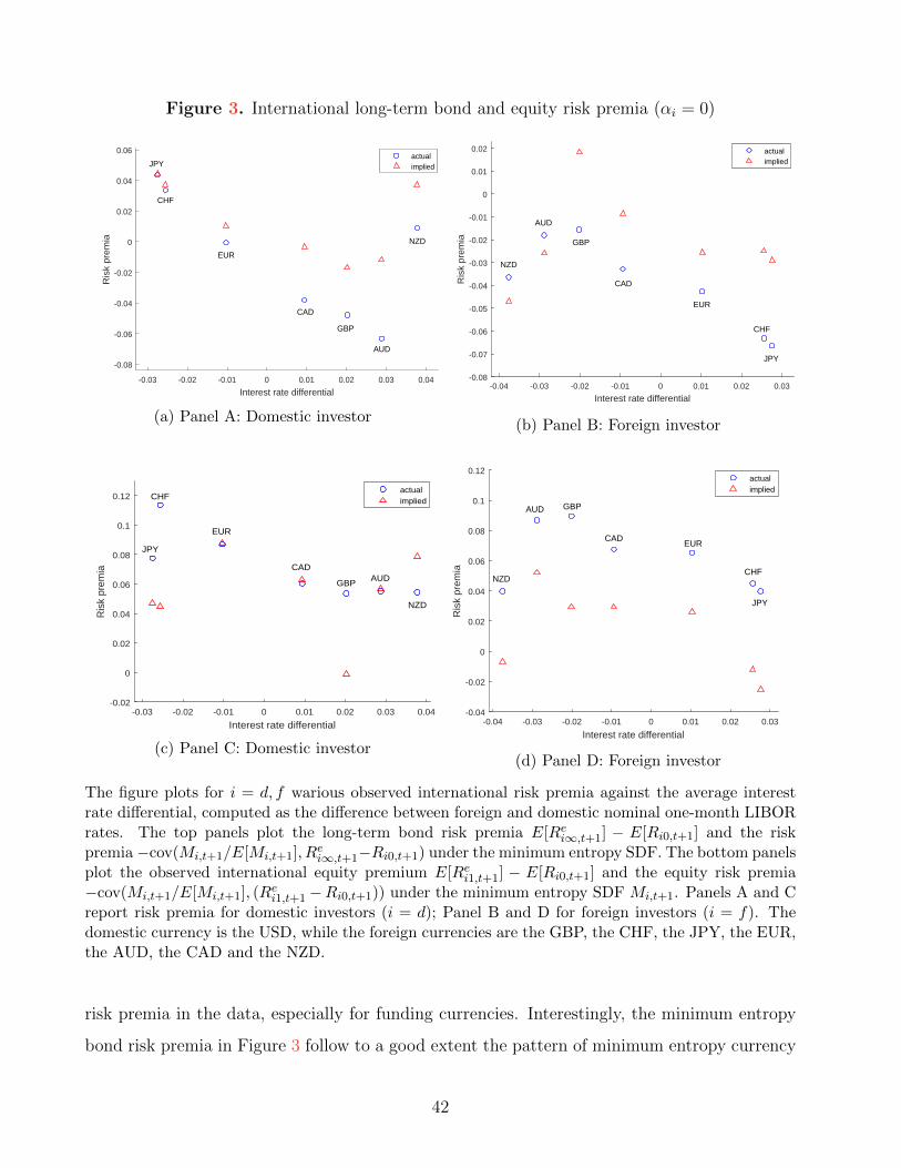
Figure 3. International long-term bond and equity risk premia (αi = 0)
-0.03 -0.02 -0.01 0 0.01 0.02 0.03 0.04
Interest rate differential
-0.08
-0.06
-0.04
-0.02
0
0.02
0.04
0.06
Ris
k pr
emia
actualimplied
CHF
EUR
JPY
CAD
GBP
AUD
NZD
(a) Panel A: Domestic investor
-0.04 -0.03 -0.02 -0.01 0 0.01 0.02 0.03
Interest rate differential
-0.08
-0.07
-0.06
-0.05
-0.04
-0.03
-0.02
-0.01
0
0.01
0.02
Ris
k pr
emia
actualimplied
NZD
AUD
GBP
CAD
EUR
CHF
JPY
(b) Panel B: Foreign investor
-0.03 -0.02 -0.01 0 0.01 0.02 0.03 0.04
Interest rate differential
-0.02
0
0.02
0.04
0.06
0.08
0.1
0.12
Ris
k pr
emia
actualimplied
JPY
CHF
EUR
CAD
GBP AUD
NZD
(c) Panel C: Domestic investor
-0.04 -0.03 -0.02 -0.01 0 0.01 0.02 0.03
Interest rate differential
-0.04
-0.02
0
0.02
0.04
0.06
0.08
0.1
0.12
Ris
k pr
emia
actualimplied
CHF
JPY
NZD
AUD GBP
CADEUR
(d) Panel D: Foreign investor
The figure plots for i = d, f warious observed international risk premia against the average interestrate differential, computed as the difference between foreign and domestic nominal one-month LIBORrates. The top panels plot the long-term bond risk premia E[Rei∞,t+1] − E[Ri0,t+1] and the riskpremia−cov(Mi,t+1/E[Mi,t+1], R
ei∞,t+1−Ri0,t+1) under the minimum entropy SDF. The bottom panels
plot the observed international equity premium E[Rei1,t+1] − E[Ri0,t+1] and the equity risk premia−cov(Mi,t+1/E[Mi,t+1], (R
ei1,t+1 −Ri0,t+1)) under the minimum entropy SDF Mi,t+1. Panels A and C
report risk premia for domestic investors (i = d); Panel B and D for foreign investors (i = f). Thedomestic currency is the USD, while the foreign currencies are the GBP, the CHF, the JPY, the EUR,the AUD, the CAD and the NZD.
risk premia in the data, especially for funding currencies. Interestingly, the minimum entropy
bond risk premia in Figure 3 follow to a good extent the pattern of minimum entropy currency
42
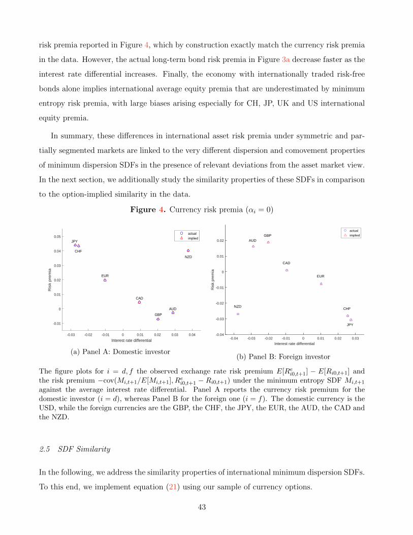
risk premia reported in Figure 4, which by construction exactly match the currency risk premia
in the data. However, the actual long-term bond risk premia in Figure 3a decrease faster as the
interest rate differential increases. Finally, the economy with internationally traded risk-free
bonds alone implies international average equity premia that are underestimated by minimum
entropy risk premia, with large biases arising especially for CH, JP, UK and US international
equity premia.
In summary, these differences in international asset risk premia under symmetric and par-
tially segmented markets are linked to the very different dispersion and comovement properties
of minimum dispersion SDFs in the presence of relevant deviations from the asset market view.
In the next section, we additionally study the similarity properties of these SDFs in comparison
to the option-implied similarity in the data.
Figure 4. Currency risk premia (αi = 0)
-0.03 -0.02 -0.01 0 0.01 0.02 0.03 0.04
Interest rate differential
-0.01
0
0.01
0.02
0.03
0.04
0.05
Ris
k p
rem
ia
actualimplied
JPY
CHF
EUR
CAD
AUD
GBP
NZD
(a) Panel A: Domestic investor
-0.04 -0.03 -0.02 -0.01 0 0.01 0.02 0.03
Interest rate differential
-0.04
-0.03
-0.02
-0.01
0
0.01
0.02
Ris
k pr
emia
actualimplied
CHF
JPY
EUR
CAD
GBPAUD
NZD
(b) Panel B: Foreign investor
The figure plots for i = d, f the observed exchange rate risk premium E[Rei0,t+1] − E[Ri0,t+1] andthe risk premium −cov(Mi,t+1/E[Mi,t+1], R
ei0,t+1 − Ri0,t+1) under the minimum entropy SDF Mi,t+1
against the average interest rate differential. Panel A reports the currency risk premium for thedomestic investor (i = d), whereas Panel B for the foreign one (i = f). The domestic currency is theUSD, while the foreign currencies are the GBP, the CHF, the JPY, the EUR, the AUD, the CAD andthe NZD.
2.5 SDF Similarity
In the following, we address the similarity properties of international minimum dispersion SDFs.
To this end, we implement equation (21) using our sample of currency options.
43
2.5.1 Option-Implied Similarity
Figure 5 plots the time-series of option-implied SDF similarity indices, using in all cases the
USD as the domestic currency, while Table 10 reports similarity summary statistics.24 We find
Figure 5. Option-Implied SDF Similarity
1994 1996 1998 2000 2002 2004 2006 2008 2010 2012
0.96
0.98
1
EU
CH
UK
1994 1996 1998 2000 2002 2004 2006 2008 2010 2012
0.96
0.98
1
CA
AU
NZ
1994 1996 1998 2000 2002 2004 2006 2008 2010 2012
0.96
0.98
1
JP
The figure plots option-implied SDF similarity measures from equation (21). Data starts in January1996 and ends in December 2013. AU = Australia, NZ = New Zealand, JP = Japan, CH = Switzerland,UK = United Kingdom, CA = Canada, EU = Eurozone. The US is always the domestic country.Gray shaded areas highlight recessions as defined by the NBER.
that option-implied similarity indices across currencies feature a large degree of co-movement
and are on average near to their upper bound of one. They exhibit interesting time-varying
and geographical patterns, with a tendency to simultaneously decrease in periods of global
financial market turmoil, such as during the recent global financial crisis. On the other hand,
is it possible that they heterogeneously react to geographically related crises, such as the Asian
crisis in 1997-1998 and the Mexican crisis of 1994-1995. The decrease in similarity during
24To take unconditional expectations as in equation (21), we can either average the values of the S(Md,Mf )directly or we can take averages for each component in the expression. Both yield very similar numbers.
44
periods of financial turmoil is a natural consequence of the progressively more expensive at-
the-money put exchange rate options; see again Proposition 3. These options offer protection
against a depreciation of the foreign currency relative to the USD. Consistent with the evidence
in Figure 5, the average option-implied SDF similarity across countries in Table 10 (Panel A)
is about 0.988 and the cross-sectional standard deviation very low.
2.5.2 Minimum Dispersion Similarity
It is interesting to compare the degree of option-implied SDF similarity to the similarity induced
by our model-free minimum entropy SDFs. To this end, recall that in general, under a deviation
from the asset market view in option data, option-implied similarities are comparable to the
SDF-based index S(Md,Mf ), but not to the SDF-based similarity S(Md,Mf ). In order to
obtain SDF-based similarity indices comparable to the option-implied indices, we convert real
minimum dispersion SDFs to nominal SDFs, by deflating real SDFs by the corresponding
inflation rate.25 We summarize the resulting numbers in Table 10 (Panel B).
We find that across all currencies, SDF-based indices S(Md,Mf ) match very closely the cor-
responding option-implied similarities in the data, independent of the assumed market segmen-
tation settings. This evidence suggests that all minimum dispersion SDFs fit unconditionally
quite accurately the put option prices embedded in index S(Md,Mf ) given in Proposition 4.
In the market setting with unrestricted trading, the SDF similarity S(Md,Mf ) closely follows
index S(Md,Mf ), because of the negligible deviations from the market view under symmetric
markets, which force international bilateral SDFs to be almost identical in order to match the
low exchange rate volatility. In contrast, the SDF similarity under internationally traded risk-
free bonds alone is clearly lower and about 0.941 on average across countries and dispersion
measures. With the exception of the CH SDF, these similarity indices are also almost identical
across dispersion measures.
2.5.3 Similarity Risk Premia
We further enlarge the set of available returns to investors by defining the return on similarity:
RdS,t+1 = 1−max(0,1−Xt+1)Bd0,t−Pd,t
, where Bd0,t and Pd,t are the domestic risk-free bond price and the put
25In the data, we find that SDF similarities computed from real and nominal SDFs are virtually identical.
45
Table 10
SDF Similarity Summary Statistics
Panel A provides descriptive statistics for SDF similarity measures computed from equation (20).Data starts in April 1993 and ends in April 2013. Panel B reports the average for the SDF similarityas implied by unrestricted international trading (I) and when international trading is restricted toshort-term bonds (II). Minimum entropy, Hellinger and variance are obtained for α = 0, α = 0.5 andα = 2, respectively. AU = Australia, NZ = New Zealand, JP = Japan, CH = Switzerland, UK =United Kingdom, CA = Canada, EU = Eurozone. The US is always the domestic country.
UK CH JP EU AU CA NZ
Panel A : Option-Implied SDF Similarity Index
Mean 0.990 0.987 0.987 0.989 0.987 0.991 0.987Std 0.003 0.003 0.004 0.004 0.005 0.004 0.005Skewness -2.624 -1.412 -1.753 -1.501 -2.810 -2.198 -1.388Kurtosis 13.85 7.449 8.982 8.143 17.39 10.21 7.321
Panel B : Nominal Minimum Dispersion SDF Similarity Index
I : Unrestricted International Trading
α = 0S(Md,Mf ) 0.991 0.987 0.989 0.988 0.987 0.991 0.987S(Md,Mf ) 0.991 0.987 0.989 0.988 0.987 0.991 0.987
α = 0.5S(Md,Mf ) 0.990 0.987 0.988 0.988 0.986 0.985 0.987S(Md,Mf ) 0.991 0.987 0.989 0.988 0.986 0.992 0.987
α = 2S(Md,Mf ) 0.990 0.986 0.989 0.988 0.986 0.990 0.987S(Md,Mf ) 0.991 0.987 0.988 0.987 0.986 0.991 0.986
II : International Trading in Short-Term Bonds Only
α = 0S(Md,Mf ) 0.952 0.928 0.945 0.971 0.961 0.973 0.949S(Md,Mf ) 0.991 0.987 0.988 0.988 0.986 0.991 0.987
α = 0.5S(Md,Mf ) 0.951 0.926 0.945 0.970 0.960 0.972 0.947S(Md,Mf ) 0.991 0.987 0.988 0.988 0.986 0.993 0.985
α = 2S(Md,Mf ) 0.950 0.921 0.944 0.970 0.959 0.971 0.947S(Md,Mf ) 0.991 0.987 0.988 0.988 0.986 0.991 0.986
46
price of an option written on the exchange rate X at time t, respectively. Next, we derive the
optimal minimum dispersion SDFs consistently, under the asymmetric setting where investors
can trade internationally the short-term bonds and the similarity return and under symmetry
where investors can trade all available assets internationally, including the similarity return.
The sample moments of the newly derived SDFs are reported in Tables 11 and 12. The
trade-off is now amplified, as trading additionally the similarity implies more volatile SDFs. To
illustrate, foreign SDFs would imply on average a 20% higher Sharpe ratio, with a maximum
(minimum) of 0.77 (0.3) registered for Switzerland (Euro-zone), whereas the domestic US SDF
also entails on average a 20% higher Sharpe ratio (Table 11, Panel A). These numbers are
even higher when investors can trade internationally all available assets. As a consequence
and consistently with the observed low volatility of the exchange rates, the correlation between
domestic and foreign SDFs increases significantly under asymmetry (Table 11) and is virtually
perfect under symmetry (Table 12).
Figure 6 plots the similarity risk premia, which is steadily increasing in the interest rate
differential. The average risk premia yields 3%, the lowest (highest) premia being encountered
for the funding (investment) currencies. This result is mirroring the currency risk premia,
which is a decreasing function of the interest rate differential. In fact, the carry strategy and
the similarity return are highly correlated. Additionally, we derive the premia implied by the
minimum entropy SDFs under asymmetry (Panel (a)) and symmetry (Panel (b)). Both settings
are underestimating the true premia, with the exception of the New Zealand. Naturally, when
we compute the implied premia using the SDFs that price the similarity return, it is going to
exactly match the observed one. We report for completeness Figure 7 in the Appendix.
We compute the similarity indices using these optimal SDFs, both for the symmetric and
asymmetric settings and report the results in Table 13. The evidence is consistent with the
estimates in Table 10, and the similarity appears to be robust across dispersion measures.
We conclude the section by computing the international risk sharing in line with the entropy-
based correlation measure defined in Chabi-Yo and Colacito (2017):
ρMf ,Md= 1− L[Mf/Md]
L[Mf ] + L[Md],
with L[x] ≡ log(E[x]) − E[log(x)] being the entropy of the positive random variable x. We
47
Table 11
Properties of SDFs (Trading in Foreign Short-Term Bonds and Similarity)
The table reports joint sample moments of the SDF and its components. Panel A reportsstatistics with respect to the minimum-entropy SDFs (αi = 0), Panel B for Hellinger SDFs(αi = 0.5) and Panel C for minimum variance SDFs (αi = 2), i = d, f , j = d, f , i 6= j. We usemonthly data from April 1993 to April 2013.
US UK US CH US JP US EU US AU US CA US NZPanel A: α = 0 (minimum entropy)
E[Mi] 0.989 0.977 0.988 0.992 0.989 0.995 0.993 0.989 0.988 0.971 0.988 0.983 0.988 0.963Std(Mi) 0.612 0.499 0.686 0.772 0.598 0.442 0.435 0.298 0.564 0.497 0.632 0.596 0.551 0.611Std(MT
i ) 0.094 0.080 0.094 0.058 0.094 0.062 0.094 0.064 0.094 0.098 0.094 0.073 0.094 0.088Std(MP
i ) 0.642 0.531 0.718 0.767 0.623 0.404 0.450 0.333 0.600 0.572 0.706 0.628 0.584 0.713√Entropy(Mi) 0.570 0.465 0.596 0.694 0.553 0.423 0.407 0.289 0.496 0.466 0.516 0.500 0.493 0.516
corr(MTi ,MP
i ) -0.308 -0.417 -0.299 0.076 -0.315 0.501 -0.227 -0.576 -0.371 -0.701 -0.315 -0.217 -0.291 -0.775corr(Mi,Mj) 0.657 0.526 0.482 0.750 0.743 0.923 0.514
Panel B: α = 0.5 (Hellinger)
E[Mi] 0.990 0.977 0.988 0.992 0.990 0.995 0.993 0.990 0.988 0.971 0.988 0.983 0.988 0.963Std(Mi) 0.601 0.494 0.657 0.751 0.585 0.438 0.428 0.297 0.544 0.490 0.603 0.572 0.535 0.570Std(MT
i ) 0.094 0.080 0.094 0.058 0.094 0.062 0.094 0.064 0.094 0.098 0.094 0.073 0.094 0.088Std(MP
i ) 0.630 0.525 0.687 0.747 0.610 0.400 0.441 0.331 0.579 0.564 0.667 0.599 0.566 0.664√Hellinger(Mi) 0.578 0.461 0.611 0.707 0.560 0.427 0.412 0.292 0.507 0.471 0.534 0.516 0.503 0.528
corr(MTi ,MP
i ) -0.309 -0.417 -0.306 0.079 -0.319 0.511 -0.224 -0.572 -0.378 -0.709 -0.328 -0.220 -0.292 -0.831corr(Mi,Mj) 0.649 0.534 0.498 0.744 0.738 0.922 0.535
Panel C: α = 2 (minimum variance)
E[Mi] 0.989 0.977 0.988 0.992 0.988 0.993 0.993 0.990 0.988 0.971 0.988 0.983 0.988 0.963Std(Mi) 0.590 0.486 0.634 0.729 0.571 0.431 0.421 0.295 0.528 0.483 0.575 0.551 0.522 0.543Std(MT
i ) 0.094 0.080 0.094 0.058 0.094 0.062 0.094 0.064 0.094 0.098 0.094 0.073 0.094 0.088Std(MP
i ) 0.619 0.517 0.661 0.725 0.596 0.398 0.434 0.329 0.563 0.555 0.619 0.572 0.550 0.624corr(MT
i ,MPi ) -0.319 -0.441 -0.321 0.071 -0.335 0.497 -0.235 -0.591 -0.393 -0.722 -0.355 -0.235 -0.305 -0.885
corr(Mi,Mj) 0.637 0.517 0.522 0.746 0.732 0.915 0.542
48
Table 12
Properties of SDFs (Unrestricted Trading and Similarity)
The table reports joint sample moments of the SDF and its components. Panel A reportsstatistics with respect to the minimum-entropy SDFs (αi = 0), Panel B for Hellinger SDFs(αi = 0.5) and Panel C for minimum variance SDFs (αi = 2), i = d, f , j = d, f , i 6= j. We usemonthly data from April 1993 to April 2013.
US UK US CH US JP US EU US AU US CA US NZPanel A: α = 0 (minimum entropy)
E[Mi] 0.989 0.977 0.988 0.992 0.988 0.993 0.993 0.990 0.988 0.971 0.988 0.983 0.988 0.963Std(Mi) 0.667 0.643 0.916 0.858 0.679 0.643 0.469 0.397 0.688 0.600 0.635 0.585 0.861 0.769Std(MT
i ) 0.094 0.080 0.094 0.058 0.094 0.062 0.094 0.064 0.094 0.098 0.094 0.073 0.094 0.088Std(MP
i ) 0.697 0.673 0.942 0.855 0.698 0.618 0.483 0.427 0.718 0.666 0.697 0.614 0.876 0.835√Entropy(Mi) 0.602 0.577 0.782 0.739 0.636 0.600 0.434 0.371 0.609 0.549 0.547 0.506 0.783 0.720
corr(MTi ,MP
i ) -0.283 -0.345 -0.223 0.060 -0.281 0.332 -0.217 -0.466 -0.317 -0.608 -0.325 -0.218 -0.184 -0.663corr(Mi,Mj) 0.990 0.992 0.987 0.978 0.980 0.991 0.985
Panel B: α = 0.5 (Hellinger)
E[Mi] 0.989 0.977 0.988 0.992 0.989 0.993 0.993 0.990 0.988 0.971 0.988 0.983 0.988 0.963Std(Mi) 0.651 0.626 0.874 0.824 0.660 0.626 0.460 0.392 0.665 0.559 0.617 0.571 0.829 0.749Std(MT
i ) 0.094 0.080 0.094 0.058 0.094 0.062 0.094 0.064 0.094 0.098 0.094 0.073 0.094 0.088Std(MP
i ) 0.679 0.656 0.899 0.823 0.680 0.602 0.473 0.421 0.695 0.653 0.673 0.597 0.845 0.813√Hellinger(Mi) 0.613 0.589 0.802 0.757 0.641 0.606 0.441 0.377 0.622 0.558 0.562 0.520 0.793
corr(MTi ,MP
i ) -0.286 -0.349 -0.230 0.063 -0.286 0.344 -0.215 -0.466 -0.322 -0.617 -0.332 -0.218 -0.188 -0.678corr(Mi,Mj) 0.989 0.991 0.986 0.975 0.981 0.991 0.985
Panel C: α = 2 (minimum variance)
E[Mi] 0.989 0.977 0.988 0.992 0.989 0.994 0.993 0.990 0.988 0.971 0.988 0.983 0.988 0.963Std(Mi) 0.634 0.610 0.836 0.791 0.640 0.610 0.452 0.387 0.644 0.576 0.598 0.552 0.788 0.724Std(MT
i ) 0.094 0.080 0.094 0.058 0.094 0.062 0.094 0.064 0.094 0.098 0.094 0.073 0.094 0.088Std(MP
i ) 0.662 0.638 0.858 0.790 0.663 0.590 0.465 0.416 0.673 0.638 0.639 0.576 0.806 0.781corr(MT
i ,MPi ) -0.289 -0.370 -0.242 0.053 -0.301 0.341 -0.224 -0.480 -0.334 -0.632 -0.350 -0.230 -0.202 -0.708
corr(Mi,Mj) 0.989 0.990 0.986 0.976 0.980 0.990 0.983
report the statistics in Table 14. As expected, whenever international financial markets are
symmetric, i.e. the asset market view holds with respect to the minimum entropy SDFs and
deviations from it are small for the remaining dispersion measures, international risk sharing is
close to being perfect. This is true in both settings where investors can trade internationally
the similarity return or not, although in the former case, the risk sharing is slightly higher.
This evidence is a direct consequence of the larger underlying dispersion of the SDFs under
symmetric settings, that in order to reconcile the low volatility of the exchange rates in the
data, need to be highly co-dependent. If one wants to diverge from perfect international risk
sharing, a form of market segmentation is required. In fact, when international long-term bonds
and stocks are segmented, which we label as asymmetry, the estimates of the risk sharing are
greatly reduced (Table 14, Panel I), especially for the funding currencies. Remarkably, trading
internationally the similarity increases the risk sharing, even in asymmetric settings (Table 14,
Panel II).
49
Table 13
Minimum Dispersion SDF Similarity Index
The table reports the average for the SDF similarity as implied by unrestricted international tradingplus similarity returns (I) and when international trading is restricted to short-term bonds plus sim-ilarity returns (II). Data starts in April 1993 and ends in April 2013. Minimum entropy, Hellingerand variance are obtained for α = 0, α = 0.5 and α = 2, respectively. AU = Australia, NZ = NewZealand, JP = Japan, CH = Switzerland, UK = United Kingdom, CA = Canada, EU = Eurozone.The US is always the domestic country.
UK CH JP EU AU CA NZ
I : Unrestricted International Trading & Similarity
α = 0S(Md,Mf ) 0.991 0.987 0.988 0.988 0.987 0.991 0.986S(Md,Mf ) 0.991 0.987 0.988 0.988 0.986 0.991 0.987
α = 0.5S(Md,Mf ) 0.990 0.987 0.988 0.988 0.987 0.990 0.985S(Md,Mf ) 0.991 0.987 0.988 0.988 0.986 0.991 0.987
α = 2S(Md,Mf ) 0.989 0.986 0.989 0.987 0.985 0.990 0.986S(Md,Mf ) 0.991 0.987 0.988 0.988 0.986 0.991 0.987
II : International Trading in Short-Term Bonds & Similarity
α = 0S(Md,Mf ) 0.951 0.931 0.946 0.969 0.962 0.974 0.949S(Md,Mf ) 0.991 0.987 0.988 0.988 0.986 0.991 0.987
α = 0.5S(Md,Mf ) 0.951 0.931 0.946 0.969 0.962 0.974 0.949S(Md,Mf ) 0.991 0.987 0.988 0.988 0.986 0.991 0.987
α = 2S(Md,Mf ) 0.951 0.931 0.946 0.969 0.962 0.974 0.949S(Md,Mf ) 0.991 0.987 0.988 0.988 0.986 0.991 0.987
50
Table 14
Risk Sharing Index
The table reports the values of the risk sharing index of Chabi-Yo and Colacito (2017), defined as
ρMf ,Md= 1 − L[Mf/Md]
L[Mf ]+L[Md], with L[x] ≡ log(E[x]) − E[log(x)] being the entropy of the positive ran-
dom variable x. The first panel reports estimates using the minimum dispersion SDFs derived wheninternational trading is restricted to short-term bonds (asymmetry) and when international trading isunrestricted (symmetry). The second panel reports estimates of the risk sharing index using minimumdispersion SDFs that price additionally the similarity return. Data starts in April 1993 and ends inApril 2013. Minimum entropy, Hellinger and variance are obtained for α = 0, α = 0.5 and α = 2,respectively. AU = Australia, NZ = New Zealand, JP = Japan, CH = Switzerland, UK = UnitedKingdom, CA = Canada, EU = Eurozone. The US is always the domestic country.
UK CH JP EU AU CA NZ
I : Minimum Dispersion SDFs
α = 0 Asymmetry 0.351 0.415 0.239 0.740 0.748 0.816 0.493Symmetry 0.983 0.988 0.980 0.962 0.979 0.982 0.982
α = 0.5 Asymmetry 0.328 0.390 0.228 0.727 0.735 0.806 0.479Symmetry 0.980 0.986 0.978 0.958 0.976 0.977 0.979
α = 2 Asymmetry 0.295 0.327 0.197 0.710 0.717 0.794 0.471Symmetry 0.977 0.982 0.952 0.955 0.964 0.975 0.817
II : Minimum Dispersion SDFs & Similarity
α = 0 Asymmetry 0.655 0.551 0.511 0.720 0.753 0.907 0.561Symmetry 0.989 0.989 0.984 0.965 0.979 0.988 0.984
α = 0.5 Asymmetry 0.635 0.533 0.507 0.707 0.740 0.907 0.548Symmetry 0.988 0.987 0.982 0.962 0.976 0.986 0.981
α = 2 Asymmetry 0.588 0.474 0.482 0.694 0.719 0.900 0.533Symmetry 0.985 0.983 0.966 0.958 0.965 0.980 0.895
51
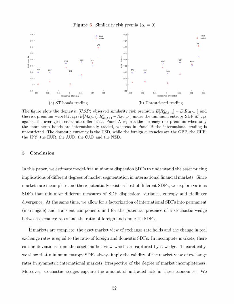
Figure 6. Similarity risk premia (αi = 0)
-0.03 -0.02 -0.01 0 0.01 0.02 0.03
Interest rate differential
-0.01
0
0.01
0.02
0.03
0.04
0.05
0.06
0.07
0.08
Ris
k p
rem
ia
actualimplied
JPY CHF
EUR
CAD
GBP AUD
NZD
(a) ST bonds trading
-0.03 -0.02 -0.01 0 0.01 0.02 0.03
Interest rate differential
-0.01
0
0.01
0.02
0.03
0.04
0.05
0.06
0.07
0.08
Ris
k p
rem
ia
actualimplied
GBP
CAD
EUR
CHFJPY
NZD
AUD
(b) Unrestricted trading
The figure plots the domestic (USD) observed similarity risk premium E[RedS,t+1] − E[Rd0,t+1] andthe risk premium −cov(Md,t+1/E[Md,t+1], R
edS,t+1−Rd0,t+1) under the minimum entropy SDF Md,t+1
against the average interest rate differential. Panel A reports the currency risk premium when onlythe short term bonds are internationally traded, whereas in Panel B the international trading isunrestricted. The domestic currency is the USD, while the foreign currencies are the GBP, the CHF,the JPY, the EUR, the AUD, the CAD and the NZD.
3 Conclusion
In this paper, we estimate model-free minimum dispersion SDFs to understand the asset pricing
implications of different degrees of market segmentation in international financial markets. Since
markets are incomplete and there potentially exists a host of different SDFs, we explore various
SDFs that minimize different measures of SDF dispersion: variance, entropy and Hellinger
divergence. At the same time, we allow for a factorization of international SDFs into permanent
(martingale) and transient components and for the potential presence of a stochastic wedge
between exchange rates and the ratio of foreign and domestic SDFs.
If markets are complete, the asset market view of exchange rate holds and the change in real
exchange rates is equal to the ratio of foreign and domestic SDFs. In incomplete markets, there
can be deviations from the asset market view which are captured by a wedge. Theoretically,
we show that minimum entropy SDFs always imply the validity of the market view of exchange
rates in symmetric international markets, irrespective of the degree of market incompleteness.
Moreover, stochastic wedges capture the amount of untraded risk in these economies. We
52
also propose a novel measure to quantify the similarity of SDF distributions which extends
well-known risk-sharing indices to incomplete and possibly segmented markets.
Using a cross-section of developed countries, we document the following novel findings. In
order to jointly explain the exchange rate puzzles, it is critical for the SDF to be factorized into a
permanent and a transient component. While we find that permanent SDF components induce
in all cases the largest fraction of SDF dispersion, we document that they are necessary to imply
an exchange rate cyclicality that is compatible with the Backus and Smith (1993) puzzle, i.e.,
the small or negative correlation between international consumption growth differentials and
exchange returns. We then show that international minimum dispersion SDFs jointly explain
the three exchange rate puzzles whenever domestic and foreign risk-free bonds can be traded
internationally.
To study the implications of different degrees of market segmentation, we explore two dif-
ferent cases: First, we give investors access to all assets in the economy: short- and long-term
bonds as well as equity indices. In the second case, we only allow them to trade the short-term
bond internationally. While both settings allow to address the exchange rate puzzles, we find
that in the former, SDF dispersion tends to be too excessive. Mild segmentation helps lower
the high dispersion.
Successful asset pricing models should therefore consist of two ingredients: Strong perma-
nent components and some form of segmentation. Segmented international currency markets
where only a subset of investors (see, e.g., Chien, Lustig, and Naknoi, 2015 and Dou and Verdel-
han (2015)) is allowed to trade all assets available and who feature non-separable utility seem
promising. Additionally, our SDF similarity indices provide these models with a tighter set of
constraints.
53
Appendix
A Proofs
Proof of Proposition 1. We study for any αi ∈ R\{1} the following minimum divergence prob-lem:26
minMi
− 1
αilogE[Mαi
i ],
subject to E(MiRi) = 1 and Mi > 0. The Lagrange function is given by
L(Mi, λi, νi) = − logE[Mαii ]
αi+ µi0E[MiRi0 − 1] +
Ki∑k=1
µikE[Mi (Rik −Ri0)] + νiMi,
with µi ∈ RKi+1 the vector of multipliers for the pricing constraints and νi the multiplier forthe positivity constraint. As the optimal SDF needs to be strictly positive, νi vanishes almostsurely and the first order conditions read:
Mαii = Mi
(µi0Ri0 +
Ki∑k=1
µik (Rik −Ri0)
)=: Miµi0Rλi ,
where we applied the renormalization λi := µik/µi0, k = 0, . . . , Ki. Taking expectations yields
E[Mαii ] = µi0. (42)
Using (42) and plugging into the first order conditions, it follows
Mi = (µi0Rλi)1/(αi−1) .
Therefore, the optimal SDF M∗i and optimal return Rλ∗i
are such that
logE[(M∗i )αi ] = logE[R
αi/(αi−1)λ∗i
]1−αi .
In summary, we get the following inequality:
− logE[Mαii ]
αi≥ − logE[M∗αi
i ]
αi=
(αi − 1)
αilogE[R
αi/(αi−1)λ∗i
] , (43)
which shows that the convexity bound implied by the optimal portfolio return Rλ∗iis tight. The
optimal SDF is given byM∗
i = R1/(αi−1)λ∗i
/E[Rαi/(αi−1)λ∗i
],
with
Rλ∗i= Ri0 +
Ki∑k=1
λ∗ik (Rik −Ri0) > 0,
26The case αi = 1 can be treated separately in a similar way, but we do not consider it here as it is notnecessary for the dispersion measures used in the main text.
54
such that for any k = 1, . . . , Ki
E[R1/(αi−1)λ∗i
(Rik −Ri0)] = 0.
Equivalently, the bound of the RHS of inequality (43) is obtained by solving the followingmaximization problem:
maxλi
(αi − 1)
αilogE[R
αi/(αi−1)λi
]
such that
Rλi =
Ki∑k=1
λik (Rik −Ri0) +Ri0 > 0.
Indeed, this optimization problem is globally strictly concave and the first order conditions fork = 1, . . . , Ki are:
0 =∂ logE[R
αi/(αi−1)λi
]
∂λi|λi=λ∗i = E[R
1/(αi−1)λ∗i
(Rik −Ri0)]. (44)
Since (44) is identical to the pricing constraints for λi in the solution of the primal SDF opti-mization problem, the bounds are tight. This concludes the proof.
Proof of Proposition 2. As (Reλ∗f
)−1 solves the moment conditions (13), it is the minimum en-
tropy SDF for return vector Ref . Hence, if (Rλ∗d
)−1 is the minimimum entropy SDF for returnvector Rd, i.e., it solves the moment condition (12), then (Re
λ∗f)−1 is the minimum entropy SDF
for return vector Ref . Symmetric arguments show that M∗e
d = (Reλ∗d
)−1 is the minimum entropySDF for return vector Re
d whenever M∗f is the minimum entropy SDF for return vector Rf .
This concludes the proof.
Proof of Proposition 3. Let the asset market view hold, i.e., X = Mf/Md. It then follows:
E[min(Md,Mf )] = E[Md min(1, X)] = E[Md]− E[Md(1−min(1, X))] .
Moreover,
E[Md(1−min(1, X))] = E[Md(1 + max(−1,−X))] = E[Md max(0, 1−X)] .
The second equality in the statement of the proposition follows by symmetry. This concludesthe proof.
Proof of Proposition 4. By definition, we have:
S(Md,MdX) =E[Md min(1, X)]
min(E[Md], E[MdX]). (45)
55

Whenever the domestic return Red0 := Rf0X is priced, it follows:
1 = Et[Md,t+1Red0,t+1] ⇐⇒
1
Rf0,t+1
= Et[Md,t+1Xt+1] , (46)
as Rf0,t+1 is the foreign risk-free rate. Taking unconditional expectations, we obtain E[MdX] =E[1/Rf0] = E[Mf ]. Therefore,
S(Md,MdX) =E[Md min(1, X)]
min(E[Md], E[Md])=E[Md]− E[Md min(0, 1−X)]
min(E[Md], E[Mf ]),
with the same arguments as in the proof of Proposition 3. By applying an identical approachwith the foreign return Re
0f := R0d(1/X), we obtain:
S(Mf ,Mf (1/X)) =E[Mf ]− E[Mf min(0, 1− (1/X))]
min(E[Md], E[Mf ]).
This concludes the proof.
Proof of Proposition 5. Given the underlying market completeness, the asset market view holdsand the exchange rate return is given by:
Xt+1 =Mf,t+1
Md,t+1
=ωdt+1/ωdtωft+1/ωft
·
ref+φHf+Hft+1
ref+φHf+Hft
red+φHd+Hdt+1
red+φHd+Hdt
. (47)
If follows that conditional on a disaster the exchange rate is:
Xt+1 =Mf,t+1
Md,t+1
= exp(gωf− gωd
)Fft+1
Fdt+1
·
ref+φHf+
1+Hf∗1+Hft
exp(−φHf)Hft
ref+φHf+Hft
red+φHd+
1+Hd∗1+Hdt
exp(−φHd)Hdt
red+φHd+Hdt
, (48)
where gωiis a constant productivity growth of country i in no-disaster times. Similarly, condi-
tional on no disasters, the exchange rate is:
Xt+1 = exp(gωf− gωd
)
ref+φHf+Hft+1
ref+φHf+Hft
red+φHd+Hdt+1
red+φHd+Hdt
, (49)
which is lognormally distributed, as it is the ratio of two jointly lognormal variables. If followsthat conditional on a no disaster event Md and X are jointly lognormal and we can apply theBlack and Scholes (1973)–Garman and Kohlhagen (1983) formula. In summary, we obtain
E[Md,t+1 max(0, 1−Xt+1)] = (1− pt)BSd(σx) + ptEDt [Md,t+1 max(0, 1−Xt+1)] ,
where EDt [·] denotes expectations conditional on a disaster event. The explicit computation of
56

the expectation on the RHS yields
EDt [Md,t+1 max(0, 1−Xt+1)] = Et
[Gd,tFd,t+1 max
(0, 1− Gf,dFf,t+1
Gd,tFd,t+1
)],
where
Gi,t = exp(gωi) ·rei + φHi
+ 1+Hi∗1+Hit
exp(−φHi)Hit
rei + φHi+ Hit
. (50)
This concludes the proof.
57
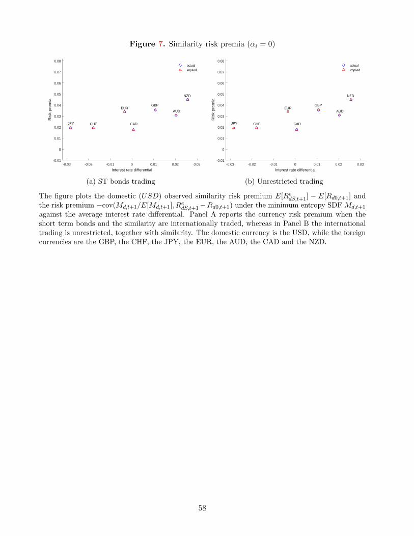
Figure 7. Similarity risk premia (αi = 0)
-0.03 -0.02 -0.01 0 0.01 0.02 0.03
Interest rate differential
-0.01
0
0.01
0.02
0.03
0.04
0.05
0.06
0.07
0.08
Ris
k p
rem
ia
actualimplied
JPY CHF CAD
GBP
AUD
NZD
EUR
(a) ST bonds trading
-0.03 -0.02 -0.01 0 0.01 0.02 0.03
Interest rate differential
-0.01
0
0.01
0.02
0.03
0.04
0.05
0.06
0.07
0.08
Ris
k p
rem
ia
actualimplied
JPY CHF CAD
GBP
AUD
NZD
EUR
(b) Unrestricted trading
The figure plots the domestic (USD) observed similarity risk premium E[RedS,t+1] − E[Rd0,t+1] andthe risk premium −cov(Md,t+1/E[Md,t+1], R
edS,t+1−Rd0,t+1) under the minimum entropy SDF Md,t+1
against the average interest rate differential. Panel A reports the currency risk premium when theshort term bonds and the similarity are internationally traded, whereas in Panel B the internationaltrading is unrestricted, together with similarity. The domestic currency is the USD, while the foreigncurrencies are the GBP, the CHF, the JPY, the EUR, the AUD, the CAD and the NZD.
58
References
Almeida, C., and R. Garcia (2012): “Assessing misspecified asset pricing models withempirical likelihood estimators.,” Journal of Econometrics, 170(2), 519–537.
Alvarez, F., A. Atkeson, and P. J. Kehoe (2009): “Time-Varying Risk, Interest Rates,and Exchange Rates in General Equilibrium,” Review of Economic Studies, 76(3), 851–878.
Alvarez, F., and U. Jermann (2005): “Using asset prices to measure the persistence of themarginal utility of wealth,” Econometrica, 73(6), 1977–2016.
Backus, D. K., S. Foresi, and C. I. Telmer (2001): “Affine term structure models andthe forward premium anomaly,” Journal of Finance, 56(1), 279–304.
Backus, D. K., and G. W. Smith (1993): “Consumption and real exchange rates in dynamiceconomies with non-traded goods,” Journal of International Economics, 35(3-4), 297–316.
Bakshi, G., M. Cerrato, and J. Crosby (2015): “Risk Sharing in International Economiesand Market Incompleteness,” Working Paper, University of Maryland.
Bakshi, G., X. Gao, and G. Panayotov (2017): “A Theory of Dissimilarity BetweenStochastic Discount Factors,” Working Paper, Univresity of Maryland.
Bansal, R., and B. N. Lehmann (1997): “Growth Optimal Portfolio Restrictions on AssetPricing Models,” Macroeconmic Dynamics, 1, 333–354.
Black, F., and M. Scholes (1973): “The Pricing of Options and Corporate Liabilities,”Journal of Political Economy, 81(3), 637–654.
Brandt, M., J. H. Cochrane, and P. Santa-Clara (2006): “International risk sharing isbetter than you think, or exchange rates are too smooth,” Journal of Monetary Economics,53(4), 671–698.
Burnside, A. C., and J. J. Graveline (2012): “On the Asset Market View of ExchangeRates,” Discussion paper, National Bureau of Economic Research.
Chabi-Yo, F., and R. Colacito (2017): “The Term Structures of Co-Entropy in Interna-tional Financial Markets,” Working Paper, University of North Carolina.
Chien, Y., H. Lustig, and K. Naknoi (2015): “Why Are Exchange Rates So Smooth? ASegmented Asset Markets Explanation,” Working Paper, Federal Reserve Bank of St. Louis.
Colacito, R., and M. M. Croce (2013): “International asset pricing with recursive prefer-ences,” Journal of Finance, 68(6), 2651–2686.
Dou, W. W., and A. Verdelhan (2015): “The Volatility of International Capital Flowsand Foreign Assets,” Working Paper, MIT.
Fama, E. F. (1984): “Forward and spot exchange rates,” Journal of Monetary Economics,14(3), 319–338.
Farhi, E., and X. Gabaix (2016): “Rare Disasters and Exchange Rates,” Quarterly Journalof Economics, 131(1), 1–52.
Gabaix, X., and M. Maggiori (2015): “International Liquidity and Exchange Rate Dy-namics,” Quarterly Journal of Economics, 130(3), 1369–1420.
59
Garman, M. B., and S. W. Kohlhagen (1983): “Foreign Currency Option Values,” Journalof International Money and Finance, 2(3), 231–237.
Hansen, L. P., and R. J. Hodrick (1980): “Forward Exchange Rates as Optimal Predictorsof Future Spot Rates: An Econometric Analysis,” Journal of Political Economy, 88(5), 829–853.
Hansen, L. P., and R. Jagannathan (1991): “Restrictions on intertemporal marginal ratesof substitution implied by asset returns,” Journal of Political Economy, 99(2), 225–62.
Kitamura, Y., T. Otsu, and K. Evdokimov (2013): “Robustness, infinitesimal neighbor-hoods, and moment restrictions,” Econometrica, 81(3), 1185–1201.
Kollmann, R. M. (1991): “Essays on International Business Cycles,” Ph.D. Thesis, Univer-sity of Chicago.
Lustig, H., A. Stathopoulos, and A. Verdelhan (2016): “Nominal Exchange RateStationarity and Long-Term Bond Returns,” Working Paper, Stanford University.
Lustig, H., and A. Verdelhan (2016): “Does Incomplete Spanning in International Finan-cial Markets Help to Explain Exchange Rates?,” Working Paper, Stanford University.
Maurer, T., and N.-K. Tran (2016): “Incomplete Asset Market View of the ExchangeRate Determination,” Working Paper, Olin Business School.
Obstfeld, M., and K. Rogoff (2001): “The Six Major Puzzles in International Macroeco-nomics: Is There a Common Cause?,” NBER Macroeconomics Annual 2000, 15, 339–412.
Orlowski, P., A. Sali, and F. Trojani (2016): “Arbitrage Free Dispersion,” WorkingPaper, University of Geneva.
Stathopoulos, A. (2017): “Asset Prices and Risk Sharing in Open Economies,” Review ofFinancial Studies, 30, 363–415.
60