Embed Size (px)
Citation preview

Model Free Subspace H∞ Control for anAutonomous Catamaran
Gabriel H. ElkaimDepartment of Computer EngineeringUniversity of California, Santa Cruz
1156 High St., Santa Cruz, CA, 95064Email: [email protected]
Bruce R. Woodley, Ph.D.Principal Systems Engineer
NeoGuide Systems Inc.104 Cooper Ct.
Los Gatos, CA 95032Email: [email protected]
Robert J. KelbleyGraduate Student Researcher
University of California, Santa Cruz1156 High St., Santa Cruz, CA, 95064
Email: [email protected]
Abstract— An autonomous surface vehicle, based on a Prindle-19 catamaran and substituting a self-trimming vertical wingfor the sail, was developed to demonstrate precision guidanceand control. This vehicle, the Atlantis, was demonstrated totrack straight line segments to better than 0.3 meters (one σ)when already trimmed to sail along a segment, using a LinearQuadratic Gaussian (LQG) controller based on an identifiedplant using the Observer Kalman Identification (OKID) methods.In this work, a novel controller based on model free subspaceH∞ control is shown to achieve similar performance levelswithout building an actual model of the system. These newcontrol methods were tested and implemented on a nonlinearsimulation of the catamaran which included realistic wind andcurrent models. The model free control architecture was appliedto the simulated catamaran and using Monte Carlo simulations,demonstrated very robust tracking traversal while maintaininga cross-track error of less than one meter throughout the path.
I. INTRODUCTION
The Atlantis, an autonomous wind-propelled catamaran, haspreviously demonstrated an accuracy better than 0.3 meters(one σ) for line following applications when already trimmedfor sail [1]. Atlantis’ guidance and control architecture hassince been extended allowing precision way-point guidedmarine navigation [2]. This paper discusses a new extensionto Atlantis’ control architecture, the addition of a novel directcontrol design methodology that provides the control responsenecessary for precision navigation in the presence of unknownwind and water current disturbances.
The connection between system identification experimentdesign and the designer’s control objectives must be taken intoconsideration when using experimental data in the control de-sign process [5]. With this connection in mind, a direct controltechnique, “model free subspace H∞ control” is applied to theAtlantis providing control design that is directly correlatedto experimental system identification data in a model freefashion.
That is, normal system identification techniques requirefirst building a mathematical model of the plant (hence thename: system identification). Using this model, a controlleris designed and tested, and then the process is repeated untilsatisfactory performance is obtained. In a model free technique(often referred to as direct controller design), the controller is
created directly from experimental data, avoiding an explicitmodel formation step.
The model free subspace H∞ control methodology utilizessubspace prediction methods directly coupled with H∞ per-formance specifications. The controller provides the Atlantiswith precision control capabilities while requiring minimalcontroller parameter tuning throughout the design process.This H∞-optimal feedback controller coupled with a way-point navigation guidance system will allow the Atlantis toperform precision, wind-propelled marine navigation whereAutonomous Surface Vehicle (ASV) capabilities are required[10].
Current results are obtained through Monte Carlo simu-lations using a nonlinear model of the Atlantis, includingrealistic wind and water current disturbances. Experimentalresults of Atlantis’ guidance and control system are expectedby the end of the year.
The key components of the Atlantis are discussed in SectionII, including previous results of precise line following control.Next, an overview of model free subspace H∞ control ispresented in Section III, followed by a discussion of thedesign parameters chosen for the Atlantis in Section IV.A comparison of LQG and H∞ controllers generated fromexperimental data is provided in Section V. The segmentedtrajectories (consisting of arcs and lines) used to connect way-points are outlined in Section VI. Monte Carlo simulationresults are presented in Section VII and finally a conclusionis provided in Section VIII.
II. THE ATLANTIS
A. System Overview
The Atlantis, pictured in Fig. 1, is an unmanned, au-tonomous, GPS-guided, wing-sailed sailboat. The Atlantis hasdemonstrated advanced precision control of a wind-propelledmarine vehicle to an accuracy of better than one meter. Theprototype is based on a modified Prindle-19 light catamaran.
The wind-propulsion system is a rigid wing-sail mountedvertically on bearings to allow free rotation in azimuth about astub-mast. Aerodynamic torque about the stub-mast is trimmedusing a flying tail mounted on booms joined to the wing.

Fig. 1. Atlantis with wing-sail, January 2001.
This arrangement allows the wing-sail to automatically at-tain the optimum angle to the wind, and weather vane intogusts without inducing large heeling moments. Modern airfoildesign allows for an increased lift to drag ratio (L/D) overa conventional sail, thus providing increased thrust whilereducing the overturning moment.
The system architecture is based on distributed sensing andactuation, with a high-speed digital serial bus connecting thevarious modules together. Sensors are sampled at 100Hz., anda central guidance navigation and control (GNC) computerperforms the estimation and control tasks at 5Hz. This band-width has been demonstrated to be capable of precise controlof the catamaran.
The sensor system uses differential GPS (DGPS) for po-sition and velocity measurements, augmented by a low-costattitude system based on accelerometer- and magnetometer-triads. Accurate attitude and determination is required to createa synthetic position sensor that is located at the center-of-gravity (CG) of the boat, rather than at the GPS antennalocation.
Previous experimental trials recorded sensor and actuatordata intended to excite all system modes. A system modelwas assembled using Observer Kalman System Identification(OKID) techniques [6]. An LQG controller was designed usingthe OKID model, using an estimator based on the observednoise statistics. Experimental tests were run to sail on a precisetrack through the water, in the presence of currents, wind, andwaves.
B. Previous Line Following Control Results
In order to validate the performance of the controllers andall up system, closed loop control experiments were performedin Redwood City Harbor, California, on January 27, 2001.These tests were intended to verify that the closed loop
controllers were capable of precise line following with theincreased disturbances due to the wing-sail propulsion. Systemidentification for the controller design was obtained previouslyusing a trolling motor as the propulsion system, in place of thewing-sail which was still under construction. No modificationswere made to the LQR controller design, and the tests wererun on a day with approximately 10 knots (or 5 m/s) of wind,with gusts up to the 16 knot (or 8 m/s) range.
Upon analyzing the data, it was demonstrated that theAtlantis was capable of sailing to within 25 degrees of thetrue wind direction. Fig. 2 presents a close-up of the first pathof regulated control, and looks at the cross-track error (Y ),azimuth error (Ψ), and velocities (V ). Note that the dark linein the top of the velocity graph is the wind speed, and can beseen to vary well over 50% of nominal.
Fig. 2. Sailing path errors.
The mean of the cross-track error is less than 3 cm., andthe standard deviation is less than 30 cm., note that this is theSailboat Technical Error (STE, the sailing analog of FlightTechnical Error). Previous characterization of the coast-guarddifferential GPS receiver indicated that the Navigation SensorError (NSE) is approximately 36 cm., thus the Total SystemError (TSE) is less than 1 meter
TSE = STE + NSE. (1)
III. MODEL FREE SUBSPACE H∞ CONTROL
A. Introduction
Subspace system identification methods have recently be-come popular for the identification of linear time invariant(LTI) systems. Initially, experimental data is used to derivea least squares optimal predictor. The predictor can then beused to derive a state space model of the dynamic system.This derivation of the state space model from the predictorcan be thought of as plant model order reduction. Instead ofusing this reduced order model for control design, model freecontrol performs the control design directly from the subspace

predictor, avoiding the formal model formation step in thedesign process.
Model free subspace H∞ control exploits this subspaceprediction method to provide a direct H∞ control designtechnique. A single, integrated algorithm computes the H∞-optimal controller and provides an estimate of the closed loopperformance. For a more thorough discussion of subspaceprediction and the model free subspace H∞ controller see[14], [15].
Fig. 3 provides an overview of the model free subspaceH∞ control design procedure. Open loop experimental datais initially used to calculate a high order predictor. Systemperformance specifications are defined using the weightingfunctions W1 and W2. The predictor and control parametersare then combined to form the controller.
Fig. 3. Model free subspace H∞ control design.
The model free subspace based H∞ control law utilizesa finite horizon cost function and is implemented with a“receding horizon” procedure. In this form, the control law isa member of a general class of controllers known as predictivecontrol. Using a future horizon of length i, at the time k theoptimal control uopt is calculated. The control at time k is thenimplemented and data yk and rk are collected. The “horizon”is then shifted one step into the future and the procedure isrepeated. The Atlantis uses a simple LTI discrete time systemto express the receding horizon controller implementation.Standard model order reduction tools can then be applied tothe LTI discrete time system if appropriate.
The reduction of the system identification step allows foran adaptive controller implementation that can adjust its per-formance specification as new closed loop input-output datais obtained. This adaptive implementation [16] will not beexplored in this paper, although its existence offers substantialmotivation for the application of these model free techniques.
As expected, the receding horizon controller implementationis derived from the H∞ performance specification and thesubspace predictor. The control design procedure can however,be viewed as a “black box” requiring the following steps:
1) Collect experimental data.2) Select i,j, and weighting functions W1,W2.3) Compute γmin and reselect W1,W2 if necessary (ideally
γmin ≤ 1). Finalize the choice of W1, W2 and chooseγ > γmin.
4) Compute and implement the final i(m + l) + nw1 +nw2 order LTI control law and apply controller orderreduction if necessary.
The following subsections outline the key elements of thisnovel control design technique. An in depth analysis of H∞control, including its advantages over H2 techniques, can befound in [7].
B. Subspace Prediction
Consider data of length n from a MIMO plant where uk ∈Rm and yk ∈ Rl, m are the number of inputs, and l arethe number of outputs. A subspace predictor can be generatedfrom this data by choosing a specific prediction horizon, i,that is larger than the expected order of the LTI plant. Thisprediction horizon is then used to break the data set into jprediction problems, where j = n−2i+1 and j � i. These jprediction problems are then used to generate the least squaresoptimal predictor Lw ∈ Ril×i(l+m) and Lu ∈ Ril×im.
Using k as the present time index, we can then use Lw andLu to predict future outputs given past experimental data andfuture inputs
yk
...yk+i−1
= Lw
uk−i
...uk−1
yk−i
...yk−1
+ Lu
uk
...uk+i−1
(2)
The derivation of Lw and Lu is reasonably straight forward.First, we define block Hankel matrices from the data using thesubscript “p” to represent “past” data and “f” to represent thecorresponding “future” data
Up ,
u0 u1 . . . uj−1
u1 u2 . . . uj
...... . . .
...ui−1 ui . . . ui+j−2
∈ Rim×j (3)
Uf ,
ui ui+1 . . . ui+j−1
ui+1 ui+2 . . . ui+j
...... . . .
...u2i−1 u2i . . . u2i+j−2
∈ Rim×j (4)
Yp ,
y0 y1 . . . yj−1
y1 y2 . . . yj
...... . . .
...yi−1 yi . . . yi+j−2
∈ Ril×j (5)
Yf ,
yi yi+1 . . . yi+j−1
yi+1 yi+2 . . . yi+j
...... . . .
...y2i−1 y2i . . . y2i+j−2
∈ Ril×j (6)

All past data can then be combined as
Wp ,
[Up
Yp
](7)
Obtaining the best linear least squares predictor of Yp givenWp and Uf can be formed as the Frobenius norm minimization
minLw,Lu
∥∥∥∥Yf −[Lw Lu
] [Wp
Uf
]∥∥∥∥2
F
(8)
The solution to this optimization problem is now given bythe orthogonal projection of the row space of Yf into therow space spanned by Wp and Uf . This orthogonal projectionsolution to (8) is given as
Yf = Yf
/[Wp
Uf
](9)
, Yf
[Wp
Uf
]T([
Wp
Uf
] [Wp
Uf
]T)† [
Wp
Uf
](10)
where † denotes the Moore-Penrose or pseudoinverse. There-fore [
Lw Lu
]= Yf
[Wp
Uf
]T([
Wp
Uf
] [Wp
Uf
]T)†
(11)
C. Model Free Subspace H∞ Control
The subspace predictor of the previous subsection will nowbe utilized to derive a finite-horizon, model free, subspacebased, H∞-optimal feedback controller. An H∞ mixed sensi-tivity criteria is used to specify the desired minimum controlperformance and desired maximum control usage. Assuming adiscrete time output unity feedback structure the specificationused is ∥∥∥∥[W1S
W2Q
]∥∥∥∥∞≤ γ (12)
where
S = (I + PK)−1 = Ger (13)
Q = K(I + PK)−1 = Gur (14)
for some plant P and controller K, and W1 and W2 areweighting functions chosen to provide the desired systemperformance. Small S up to a desired cutoff frequency cor-responds to each output tracking its reference well in the fre-quencies of interest. Limiting the magnitude of Q, especiallyat high frequencies, limits the control effort used.
The time-domain discrete-time expression for the specifica-tion in (12) is formulated as follows:
z ,
[zw1
zw2
]=[w1 ∗ ew2 ∗ u
]=[w1 ∗ (r − y)
w2 ∗ u
](15)
where w1 and w2 are the respective discrete impulse responsesof the discrete time weighting functions W1 and W2. Using(15), the finite-horizon problem of (12) can be written as
supr
J(γ) ≤ 0, where J(γ) =i−1∑t=0
(zTt zt − γ2rT
t rt) (16)
and the system is assumed to be at rest at t = 0. The lengthof the horizon, i, has been selected to be identical to theprediction horizon in the previous subsection, so (2) can beused to calculate J(γ). Using J(γ) from (16), the centralfinite-horizon H∞ controller satisfies
minu
supr
J(γ) ≤0 (17)
whenever the system is at rest at t = 0.
D. Subspace Based finite-horizon H∞ Control
Given the generalized plant of Fig. 4, the level-γ H∞control design problem is to choose a control u such thatthe finite-horizon H∞ gain from r to z is of magnitude γ.This subsection derives the condition on γ that ensures thatthe problem is feasible, and computes the central solution forthis H∞ control problem.
Fig. 4. Generalized plant for H∞ control design.
If measurements of the plant input u, plant output y, andreference r are available for times {k−i, . . . , k−2, k−1}, thenthe strictly causal, finite-horizon, model free, subspace based,level-γ, central H∞ control for times {k, . . . , k + i− 1} is
uopt = −(LTu Q1Lu + Q2)−1· (LT
u Q1Lw)T(−LT
u (γ−2Q1 + I)HT1 Γ1
)T
(HT2 Γ2)T
T wp
xw1
xw2
k
(18)
Q1 = (Q−11 − γ−2I)−1 (19)
provided that
γ > γmin ,√
λ[(Q−11 + LuQ−1
2 LTu )−1] (20)
where the discrete LTI weighting filters W1 and W2 have theminimal state space representation
(xw1)k+1 = Aw1(xw1)k + Bw1(rk − yk) (21)(zw1)k = Cw1(xw1)k + Dw1(rk − yk) (22)
(xw2)k+1 = Aw2(xw2)k + Bw2(uk) (23)(zw2)k = Cw2(xw2)k + Dw2(rk − yk) (24)
The lower triangular Toeplitz matrices H1 and H2 areformed from the Markov parameters of the discrete weightingfilters W1 and W2
H1 ,
Dw1 . . . 0 . . . 0
Cw1Bw1 . . . 0 . . . 0Cw1Aw1Bw1 . . . Dw1 . . . 0
......
. . ....
Cw1Ai−2w1
Bw1 . . . Cw1Ai−4w1
Bw1 . . . Dw1
(25)
H2 ,
pDw2 . . . 0 . . . 0
Cw2Bw2 . . . 0 . . . 0Cw2Aw2Bw2 . . . Dw2 . . . 0
......
. . ....
Cw2Ai−2w2
Bw2 . . . Cw2Ai−4w2
Bw2 . . . Dw2
(26)
and
Q1 , HT1 H1 , Q2 , HT
2 H2 (27)
The extended observability matrices that contain the weightingfilter impulse responses are defined as
Γ1 ,
Cw1
Cw1Aw1
...Cw1A
i−1w1
, Γ2 ,
Cw2
Cw2Aw2
...Cw2A
i−1w2
(28)
and vector of past plant inputs and outputs is defined as
(wp)k ,
uk−i
...uk−1
yk−i
...yk−i
. (29)
E. MFSH∞ Predictive Control
The final step of the control design procedure, the recedinghorizon implementation, is expressed as the following MIMOLTI discrete time system :
up
yp
xw1
xw1
k+1
=
[Sm
k1
] [0k2
] [0k3
] [0k4
]0
[Sl
0
]0 0
0 0 Aw1 0Bw2k1 Bw2k2 Bw2k3 Aw2 + Bw2k4
up
yp
xw1
xw1
k
+
0 0
0[0Il
]Bw1 Bw1
0 0
[ry
]k
(30)
uk =[k1 k2 k3 k4
] up
yp
xw1
xw2
k
(31)
where uk ∈ Rm, rk ∈ Rl, yk ∈ Rl, m are the number of plantinputs, and l are the number of plant outputs. Im and Il aredefined as m×m and l × l identity matrices respectively,
Sm =
0 Im 0 . . . 00 0 Im . . . 0...
......
. . . 00 0 0 . . . Im
∈ R(i−1)m×im (32)
Sl =
0 Il 0 . . . 00 0 Il . . . 0...
......
. . . 00 0 0 . . . Il
∈ R(i−1)l×il (33)
and[k1 k2
]={−(LT
u Q1Lu + Q2)−1LTu Q1Lw
}1:m,:
(34)
k3 ={
(LTu Q1Lu + Q2)−1LT
u (γ−2Q1 + I)HT1 Γ1
}1:m,:
(35)
k4 ={−(LT
u Q1Lu + Q2)−1HT2 Γ2
}1:m,:
(36)
where {•}1:m,: means extract the first m rows of the matrix •,and k1 ∈ Rm×im, k2 ∈ Rm×il, k3 ∈ Rm×nw1 , k4 ∈ Rm×nw2 .
IV. ATLANTIS CONTROLLER DESIGN PARAMETERS
A. Subspace Prediction Horizon
As discussed in Section III, the subspace predictor isgenerated using experimental input-output data of length n.A prediction horizon, i, is then chosen that breaks the data setinto j prediction problems, where j = n−2i+1. To ensure anaccurate predictor is created for a LTI model, i will be chosento be at least twice as large the expected plant order.
The simulated system identification data used to generatethe subspace predictor is shown in Fig. 5. The boat uses rudder

slew rate (δ) as the input signal and has three output signals:cross-track (Y ), azimuth (Ψ), and effective rudder angle (δ).
Fig. 5. Simulated open loop system identification data created by controllingthe slew rate of the Atlantis with a pseudo-random binary sequence.
Although the Atlantis is a nonlinear system, Section IIshows that LQG techniques are effective for precision controlwhen small azimuth and cross-track deviations are maintained.To generate a more accurate predictor a high order predictionhorizon was used by choosing i = 100. Fig. 6 shows thepredictor generated is adequate at predicting Atlantis’ responseto a known input. This particular data was from a simulatedsystem identification pass similar to that shown in Fig. 5,however, this data was not used in generating the subspacepredictor.
Fig. 6. The subspace predictor reconstruction of a simulated systemidentification pass comparing measured outputs to predicted values.
B. Mixed Sensitivity Cost Function
As shown in Section III, W1 and W2 are weighting functionschosen to provide the desired system performance for themixed sensitivity criteria given in (12). It is important tonote that increasing either the DC gain or bandwidth of W1
will make the controller more aggressive. This will forcethe controller to track higher error signal frequencies makingthe response faster, but less damped. Decreasing W2 willpermit greater control usage, which is typically not desirableat high frequencies. However, if W1 is increased, requestinghigher performance, but W2 is not sufficiently decreased, toprovide more control usage, the problem will become overconstrained. These over lapping constraints will be reflectedby γopt increasing over the nominal value of one. W1 and W2
were then selected with these performance tradeoffs in mind.
Fig. 7. Control Specification for Atlantis. Note all three control inputs usethe identical cost function W−1
1 .
Fig. 7 shows the inverse of each weighting function chosenfor the Atlantis. Identical W1 functions were used to specifythe performance requirements for Y , Ψ, and δ. As shown, thedesign cutoff frequency is around 0.9 rad/sec (0.14 Hz). It isdesirable that all three outputs stay nominally around zero toprovide a more linear response of the system, therefore 6 dB ofrejection at DC was chosen. The control usage function, W2,which effects the slew rate of the rudders was then selectedto provide sufficient control usage to meet the performancespecifications while staying within the limitations of the rudderactuator system.
A value of γ was selected that would provide fairly ag-gressive closed loop response while allowing some margin tomaintain stability. The smallest achievable γ value, γmin, wascalculated to be 1.81 based on the previously described predic-tor and weighting functions. We then chose γ = (1.5)γmin =2.71 which is later shown to meet our controller requirements.
C. Model Order Reduction
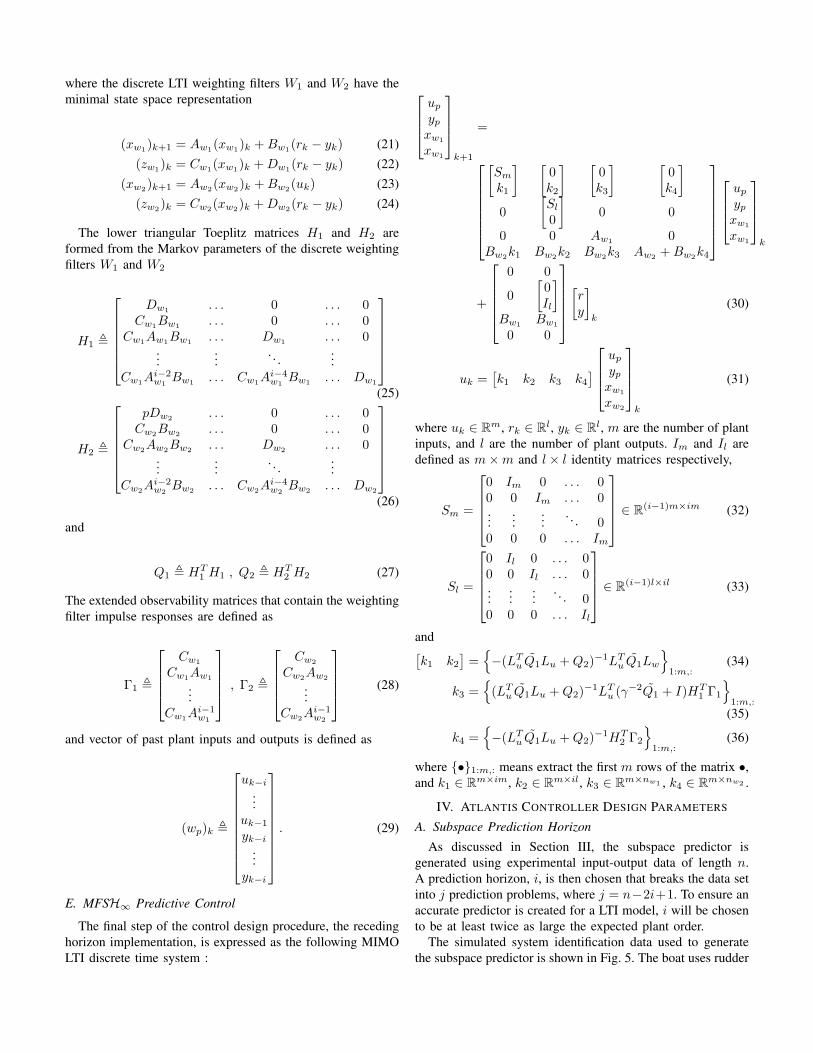
Initially, a high order predictor was used to provide asmuch information as possible for the controller design. Thecontroller generated using the high order subspace predictortherefore also had a substantially high order. Fig. 8 shows theHankel singular values of the controller generated from thesubspace predictor, weighting functions, and γ value.
The first five singular values of the Hankel matrix standout, therefore it is assumed the controller can be reduced
to a fifth order system. A balanced realization was thenused to truncate the controller at the desired order. Thisassumption was verified by simulating controllers of variousorders. Results showed that keeping modes higher than fivedid not noticeably effect system performance.
Fig. 8. Hankel Singular Value plot of initial controller design. Note the dropoff in the singular values after the fifth one, indicating a system of order five.
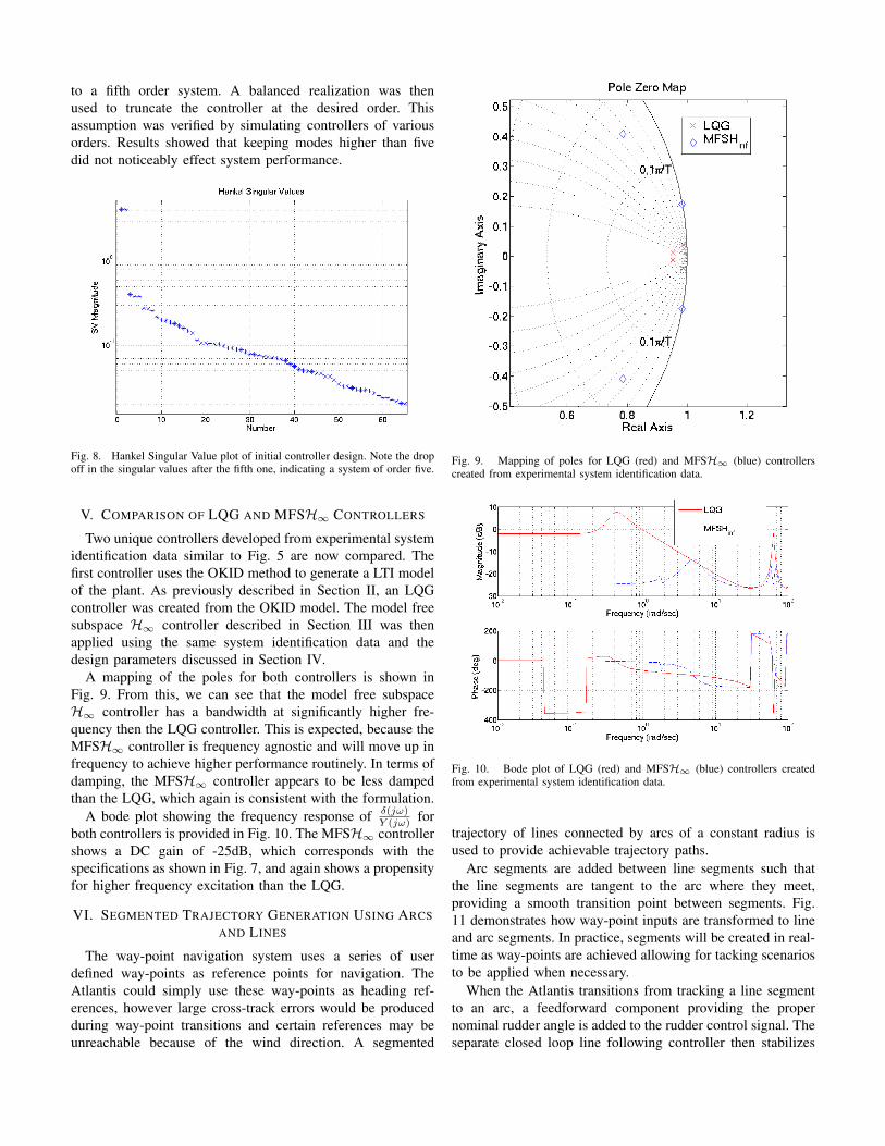
V. COMPARISON OF LQG AND MFSH∞ CONTROLLERS
Two unique controllers developed from experimental systemidentification data similar to Fig. 5 are now compared. Thefirst controller uses the OKID method to generate a LTI modelof the plant. As previously described in Section II, an LQGcontroller was created from the OKID model. The model freesubspace H∞ controller described in Section III was thenapplied using the same system identification data and thedesign parameters discussed in Section IV.
A mapping of the poles for both controllers is shown inFig. 9. From this, we can see that the model free subspaceH∞ controller has a bandwidth at significantly higher fre-quency then the LQG controller. This is expected, because theMFSH∞ controller is frequency agnostic and will move up infrequency to achieve higher performance routinely. In terms ofdamping, the MFSH∞ controller appears to be less dampedthan the LQG, which again is consistent with the formulation.
A bode plot showing the frequency response of δ(jω)Y (jω) for
both controllers is provided in Fig. 10. The MFSH∞ controllershows a DC gain of -25dB, which corresponds with thespecifications as shown in Fig. 7, and again shows a propensityfor higher frequency excitation than the LQG.
VI. SEGMENTED TRAJECTORY GENERATION USING ARCSAND LINES
The way-point navigation system uses a series of userdefined way-points as reference points for navigation. TheAtlantis could simply use these way-points as heading ref-erences, however large cross-track errors would be producedduring way-point transitions and certain references may beunreachable because of the wind direction. A segmented
Fig. 9. Mapping of poles for LQG (red) and MFSH∞ (blue) controllerscreated from experimental system identification data.
Fig. 10. Bode plot of LQG (red) and MFSH∞ (blue) controllers createdfrom experimental system identification data.
trajectory of lines connected by arcs of a constant radius isused to provide achievable trajectory paths.
Arc segments are added between line segments such thatthe line segments are tangent to the arc where they meet,providing a smooth transition point between segments. Fig.11 demonstrates how way-point inputs are transformed to lineand arc segments. In practice, segments will be created in real-time as way-points are achieved allowing for tacking scenariosto be applied when necessary.
When the Atlantis transitions from tracking a line segmentto an arc, a feedforward component providing the propernominal rudder angle is added to the rudder control signal. Theseparate closed loop line following controller then stabilizes

Fig. 11. User defined way-points (top) transformed into arc and line segments(bottom).
the system around this nominal rudder angle for a giventurning radius. The feedforward term is removed once the arcis traversed and the new line segment is being tracked.
VII. SIMULATION RESULTS
A nonlinear model of the Atlantis which includes windand wave disturbances was previously developed in [2]. Thismodel, combined with the way-point navigation system de-scribed in Section VI was then used in Monte Carlo sim-ulations to compare three different controllers designed forprecise trajectory tracking in the presence of environmentaldisturbances. Each controller monitors azimuth (Ψ), cross-track (Y ), and rudder position (δ) to adjust the rudder slewrate (δ). The first controller simulated is the PID controllerdescribed in [2]. Next the LQG controller developed in [1]was simulated. Finally, the model free subspace H∞ controllerdeveloped in Section IV was tested.
The set of way-points shown in Fig. 12 were selected andMonte Carlo simulations were run for 100,000 seconds foreach of the three different controllers, with random windand water disturbance conditions provided for each trial. Theresults obtained are shown in Table I, the model free subspaceH∞ controller obtained the smallest combination of total aver-age cross-track error and cross-track error standard deviation.Fig. 13 shows the resulting cross-track and azimuth error datafrom an average simulated run. Monte Carlo simulation resultsshow the Atlantis having an average cross-track error of 8 cmwith a standard deviation of 65 cm when using the model freesubspace H∞ controller.
Fig. 12. Control architecture applied to wing-sailed vehicle simulated withwater current and wave disturbances.
Fig. 13. Azimuth and cross-track error for wing-sailed surface vehiclesimulation.
TABLE ISIMULATION RESULTS.
PID LQG MFSH∞Lines Total Lines Total Lines Total
Y (cm) 20 27 1 8 2 8Yσ(cm) 49 59 61 75 56 65Y + Yσ(cm) 69 86 62 84 58 73
Analysis of the simulation results shows that all threecontrollers perform comparably for straight line segments.However, the disturbances introduced by the addition of arcsegments produced greater errors for the PID and LQG con-trollers. The MFSH∞ controller performed more than 10%better than the other controllers within the complete segmentedtrajectory guidance system, even though considerably lesstuning of control parameters was necessary for the MFSH∞controller.

VIII. CONCLUSIONS
A control architecture for an autonomous sailboat using away-point navigation system was simulated using a modelfree subspace H∞ controller and shown capable of providingrobust and reliable guidance under realistic wind and waterdisturbance models. This architecture was applied to a sim-plified model of the Atlantis, a wing-sail propelled catamaranpreviously shown capable of line following accuracy betterthan 0.3 meters. Simulations modeling similar experimentalconditions previously encountered show that precision controlis possible for way-point navigation requiring segmented tra-jectory following of arcs and lines and real-time way-pointmanagement to prevent unreachable points of sail.
Simulations show the sailboat can be controlled to betterthan one meter of accuracy, providing similar performanceto previous experimental results using an LQG controller.However, a key difference is the model free subspace H∞controller reduces the complexity of the control design processby eliminating the standard model formation step. This directcontrol design methodology has also been demonstrated toperform exceptionally well when used in an adaptive controllerimplementation. Application of this adaptive control techniquewill be the focus of future precision control research for theAtlantis. Experimental validation is expected within the nextyear.
Other future work will include a way-point generationmethodology that will avoid stationary obstacles and also opti-mally determine trajectories given only a destination point andweather data forecasts to predict future wind and wave activity.This added guidance system combined with advancements inAtlantis sensors and actuators will create a wind-propelledASV capable of robust navigation.
REFERENCES
[1] G.H. Elkaim. System Identification for Precision Control of a WingsailedGPS-Guided Catamarn. PhD thesis, Stanford University, 2001.
[2] G.H. Elkaim and R.J. Kelbley. Control architecture for segmentedtrajectory following of a wind-propelled autonomous catamaran. AIAAGuidance, Navigation, and Control Conference, August 2006.
[3] P. Encarnacao, A. Pascoal, and M. Arcak. Path following for autonomousmarine craft. 5th IFAC Conference on Maneuvering and Control ofMarine Craft, pages 117–22, 2000.
[4] T.I. Fossen. Guidance and Control of Ocean Vehicles. Wiley and Sons,New York, NY, 1994.
[5] M. Gevers. Identification for control: From the early achievements to therevival of experiment design. European Journal of Control, 11:335–352,2005.
[6] J.-N. Juang. Applied System Identification. Prentice Hall, NJ, 1994.[7] K.Zhou. Robust and Optimal Control. Prentice-Hall, Inc., Upper Saddle
River, NJ, 1996.[8] E. Lefeber, KY. Pettersen, and H. Nijmeijer. Tracking control of an
underactuated ship. IEEE Transactions on Control Systems Technology,3:52–61, January 2003.
[9] B.W. McCormick. Aerodynamics, Aeronautics, and Flight Mechanics.John Wiley and Sons, New York, NY, 1979.
[10] A. Pascoal, P. Olivera, and C. Silvestre. Robotic ocean vehicles formarine science applications: The european asimov project. OCEANS2000 MTS/IEEE Conference and Exhibition, 1:409–415, 2000.
[11] R.S.Shevell. Fundamentals of Flight. Prentice-Hall, Inc., EnglewoodCliffs, NJ, 1983.
[12] R. Skjetne and T. Fossen. Nonlinear maneuvering and control of ships.MTS/IEEE OCEANS 2001, 3:1808–15, 2001.
[13] T. VanZwieten. Dynamic Simulation and Control of an AutonomousSurface Vehicle. PhD thesis, Florida Atlantic University, 2003.
[14] B.R. Woodley. Model Free Subspace Based H∞ Control. PhD thesis,Stanford University, 2001.
[15] B.R. Woodley, J.P. How, and R.L. Kosut. Model free subspace basedH∞ control. Proceedings of the American Control Conference, pages2712–2717, 2001.
[16] B.R. Woodley, J.P. How, and R.L. Kosut. Subspace based direct adaptiveH∞ control. Int. J. Adapt. Control Signal Process, 15:535–561, 2001.