Model independent constraints on the cosmological ...redshift, considerably relaxed the constraints on the expansion history. Speci cally, using the so called \gold" dataset consisting

$Page 1: Model independent constraints on the cosmological ...redshift, considerably relaxed the constraints on the expansion history. Speci cally, using the so called \gold" dataset consisting$
Model independent constraints on the cosmological

expansion rate

Edvard Mortsell1 and Chris Clarkson2

1 Department of Physics, Stockholm University, AlbaNova University CenterS–106 91 Stockholm, Sweden2 Cosmology and Gravity Group, Department of Mathematics and AppliedMathematics, University of Cape Town, Rondebosch 7701, Cape Town, South Africa

E-mail: [email protected], [email protected]

Abstract. We investigate what current cosmological data tells us about thecosmological expansion rate in a model independent way. Specifically, we study if theexpansion was decelerating at high redshifts and is accelerating now, without referringto any model for the energy content of the universe, nor to any specific theory ofgravity. This differs from most studies of the expansion rate which, e.g., assumes someunderlying parameterised model for the dark energy component of the universe. Toaccomplish this, we have devised a new method to probe the expansion rate withoutrelying on such assumptions.

Using only supernova data, we conclude that there is little doubt that the universehas been accelerating at late times. However, contrary to some previous claims, we cannot determine if the universe was previously decelerating. For a variety of methods usedfor constraining the expansion history of the universe, acceleration is detected fromsupernovae alone at > 5σ, regardless of the curvature of the universe. Specifically,using a Taylor expansion of the scale factor, acceleration today is detected at > 12σ.If we also include the ratio of the scale of the baryon acoustic oscillations as imprintedin the cosmic microwave background and in the large scale distribution of galaxies,it is evident from the data that the expansion decelerated at high redshifts, but onlywith the assumption of a flat or negatively curved universe.

Keywords: dark energy theory, supernova type Ia

1. Introduction

It is becoming generally acknowledged that the observed redshift-distance relation from

Type Ia supernovae (SNe Ia), together with the scales of baryon acoustic oscillations as

observed in the distribution of galaxies on large scales (BAO) and the temperature

anisotropies in the cosmic microwave background (CMB), implies that the current

energy density in the universe is dominated by dark energy, here defined as a component

with an equation of state, w = p/ρ < −1/3. Current cosmological data are consistent

with the standard – or concordance – cosmological model, where Ωm = 0.3 and ΩΛ = 0.7,

i.e., the dark energy is explained in terms of a cosmological constant or vacuum energy

with w = −1 [e.g., 1, 11, 15, 16, 24, 35]. For the concordance model, the universal

arX

iv:0

811.

0981

v2 [

astr

o-ph

] 2

8 Ja

n 20

09

Model independent constraints on the cosmological expansion rate 2

expansion is accelerating at redshifts lower than z ∼ 0.7 and decelerating at higher

redshifts.

Most analyses which attempt to infer something about the expansion history of the

universe rely on a specific model, e.g., a dark energy ‘fluid’ or a modification of general

relativity, which has one or two parameters of interest [13]. Consequently, much of our

knowledge of the expansion history of the universe has these parameterisations hard-

wired into our conclusions, which may leave a large space of possible expansion histories

unexplored. Alongside these analyses, it is therefore constructive to try to assert model

independent statements where we can. The question we address in this paper is to what

extent we can infer changes in the expansion rate without referring to any theory of

gravity or model for the energy content of the universe. That is; what is the history of

the universal expansion?

Unfortunately, it is difficult to give a definite answer to this question since two

important assumptions are implicit in all discussion of this kind. It is known that

spherically symmetric void – or Hubble bubble – models may explain the anomalous

Hubble diagram whilst always maintaining a decelerating expansion rate, at the price

of violating the Copernican principle [3, 4, 6, 10, 18, 19, 20, 38, 46, 48]. Ideally

we should test the Copernican principle in a model independent way [8, 45], and

so rule these models out. A further assumption in the standard model – insofar as

determining the expansion dynamics is concerned – is that that the universe is smooth

enough at small distances to be described by a perfectly homogeneous and isotropic

model [2, 5, 12, 26, 27, 28, 32, 33, 37, 41]. At best this gives a small error to all our

considerations; at worst, many of our conclusions might be wrong.

Since it was traditionally thought that the expansion rate would be decelerating,

we measure acceleration with the deceleration parameter, q, defined by

q ≡ − aaa2

= − a

aH2, (1)

where a is the scale factor, dots denote derivatives with respect to time and the Hubble

parameter, H, is defined as H ≡ a/a. Because of the sign convention, negative values for

q correspond to acceleration. Traditionally, the goal when observing the expansion of the

universe was to constrain two parameters, the current values of the Hubble parameter

– or the Hubble constant – H0, and the deceleration parameter, q0. The first signs

of an accelerated expansion came 10 years ago with the observations that distant SN

Ia appear dimmer than expected in a universe with constant or decelerated expansion

velocity [30, 34, 39]. However, the acceleration was only evaluated in terms of a model

with Ωm and ΩΛ, in which q0 = Ωm/2− ΩΛ, see Eq. (4).

In 2002, Turner and Riess [44] studied the change in the expansion velocity –

without referring to the energy content or theory of gravity – by using a step model

for the deceleration parameter where q had one constant value at low and intermediate

redshifts and another constant value at high redshifts. They demonstrated, that the SN

Ia data at the time showed a strong preference for acceleration today and deceleration

in the past, if the transition redshift was set (by hand) to z = 0.4− 0.6. However, this


conclusion relied heavily on the observed magnitude of a single supernova, SN1997ff,

the most distant SN Ia observed at z = 1.755. Being very distant, it is especially

susceptible to systematic effects that may reduce its cosmological utility. One such

effect is gravitational lensing that has been shown to brighten SN1997ff by ∼ 0.15

magnitudes [23].

Also, in Shapiro and Turner [43], it was shown that marginalising over the transition

redshift, considerably relaxed the constraints on the expansion history. Specifically,

using the so called “gold” dataset consisting of 157 SNe Ia [36], the authors only found

strong evidence for acceleration at some epoch, not necessarily at z < 0.1, and that q

was higher in the past.

In 2004, Riess et al. [36], the gold dataset was used to constrain a Taylor expansion

of q(z),

q(z) = q0 + zq′(z = 0) , (2)

where the prime denotes a derivative with respect to redshift. The result found was

that q0 . −0.3 and q′ & 0 at 95 % confidence level (CL). The evidence that q′ & 0,

was interpreted as evidence for deceleration at higher redshifts. However, the Taylor

expansion should only be meaningful for z < 1, up to which the parameter space [q0, q′]

still allows for acceleration at 95 % CL. Also, the fit is done using data at z > 1, for

which higher order terms in the Taylor expansion should be important.

In, Elgarøy and Multamaki [17], the same data was found to be consistent with

a constant negative deceleration parameter, and in Rapetti et al. [31], the SN data

was combined with X-ray cluster gas mass fraction measurements to constrain the

deceleration parameter, q, as well as the next order derivative of the scale factor as

decoded in the jerk parameter, j. See also Daly et al. [14] for an alternative approach

to constraining the acceleration history of the universe.

In this paper, we follow the spirit of previous work, in that we strive to make

as few assumptions as possible regarding the theory of gravity or the energy content

of the universe when inferring the state of the expansion velocity of the universe. In

fact, the only assumptions used in this paper, other than those mentioned, is that SNe

Ia are standardisable candles and that the observed inhomogeneities in the large scale

distribution of galaxies and the anisotropies in the temperature of the CMB reflects

the same physical scale. One feature we discuss in particular is the role of curvature

in determining the acceleration, as there are significant degeneracies between curvature

and acceleration, in a similar vein which exists between curvature and the dark energy

equation of state w [9, 21].

In Sec. 2, we discuss acceleration and deceleration within the standard model, as

well as possible observational measures of the deceleration parameter. In Sec. 3, we

present the two sources of data used in this paper, and in Sec. 4, we present a new

method for inferring the expansion history of the universe, together with our results for

q(z). Our results are summarised in Sec. 5. In short, we conclude that the evidence for

late time acceleration of the universal expansion is very strong, regardless of the method


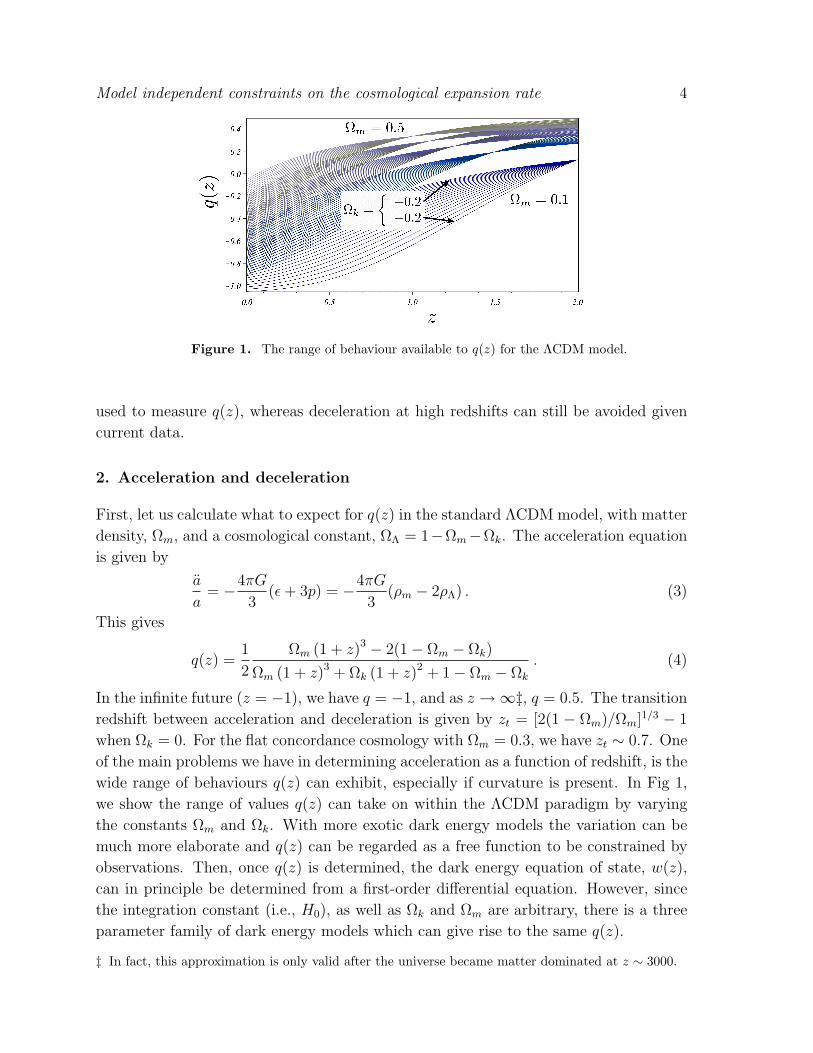
Figure 1. The range of behaviour available to q(z) for the ΛCDM model.

used to measure q(z), whereas deceleration at high redshifts can still be avoided given

current data.

2. Acceleration and deceleration

First, let us calculate what to expect for q(z) in the standard ΛCDM model, with matter

density, Ωm, and a cosmological constant, ΩΛ = 1−Ωm−Ωk. The acceleration equation

is given by

a

a= −4πG

3(ε+ 3p) = −4πG

3(ρm − 2ρΛ) . (3)

This gives

q(z) =1

2

Ωm (1 + z)3 − 2(1− Ωm − Ωk)

Ωm (1 + z)3 + Ωk (1 + z)2 + 1− Ωm − Ωk

. (4)

In the infinite future (z = −1), we have q = −1, and as z →∞‡, q = 0.5. The transition

redshift between acceleration and deceleration is given by zt = [2(1 − Ωm)/Ωm]1/3 − 1

when Ωk = 0. For the flat concordance cosmology with Ωm = 0.3, we have zt ∼ 0.7. One

of the main problems we have in determining acceleration as a function of redshift, is the

wide range of behaviours q(z) can exhibit, especially if curvature is present. In Fig 1,

we show the range of values q(z) can take on within the ΛCDM paradigm by varying

the constants Ωm and Ωk. With more exotic dark energy models the variation can be

much more elaborate and q(z) can be regarded as a free function to be constrained by

observations. Then, once q(z) is determined, the dark energy equation of state, w(z),

can in principle be determined from a first-order differential equation. However, since

the integration constant (i.e., H0), as well as Ωk and Ωm are arbitrary, there is a three

parameter family of dark energy models which can give rise to the same q(z).

‡ In fact, this approximation is only valid after the universe became matter dominated at z ∼ 3000.


Normalising the scale factor to be unity today, a = (1 + z)−1, we may derive

z = −(1 + z)H, and

q(z) = − H

H2− 1 =

H ′

H(1 + z)− 1 = (1 + z)

[ln

H

1 + z

]′. (5)

In principle, Eq. (5) can be used to obtain the value of the deceleration parameter as a

function of redshift. Unfortunately, it is very difficult to measure the Hubble parameter,

H(z), let alone its derivative. As an example, from Fig. 3, it can be understood why it

is difficult to differentiate noisy SN Ia data in order to obtain H(z). Note however that

with future BAO data, it may be possible to measure H(z) directly [42].

Rearranging Eq. (5), we can write

H ′

H=

1 + q(z)

1 + z→∫ z2

z1

d(lnH)

dzdz =

∫ z2

z1

1 + q(z)

1 + zdz . (6)

If the universe is accelerating between redshifts z1 and z2, we have

ln

(H2

H1

)< ln

(1 + z2

1 + z1

)→ (1 + z2)

H2

>(1 + z1)

H1

. (7)

When we have acceleration, H(z) thus grows with redshift faster than (1 + z). This is

easy to understand since if a = H/(1 + z) is increasing with redshift, a is decreasing

with time and a < 0, corresponding to acceleration. For deceleration, H(z) grows slower

than (1 + z). For a matter dominated universe, H = H0

√Ωm(1 + z)3 ∝ (1 + z)1.5, i.e.,

the expansion is decelerating. For an empty universe, H = H0

√Ωk(1 + z)2 ∝ (1 + z),

i.e., the expansion velocity is constant. Note however that an empty universe is not the

only possible solution for a constant expansion velocity – any universe where the total

energy density scales as (1 + z)2 also gives a constant expansion.

The comoving coordinate distance is given by

dc(z) =

∫ z

0

dz

H(z)=

1

H0

∫ z

0

exp

[−∫ v

0

[1 + q(u)]du

(1 + u)

]dv , (8)

and the luminosity distance, which is the relevant quantity for SN Ia observations, is

given by

dL(z) =1 + z

H0

√−Ωk

sin[√−ΩkH0dc(z)

]. (9)

The angular diameter distance, relevant for the scale of BAO and CMB, is given by

dA = dL/(1+z)2. Although having the same constant expansion rate, we would therefore

measure different luminosity and angular diameter distances in the flat and open non-

accelerating cases. Determining acceleration at a given redshift is then the same as

determining if the function [(1+z)D′/H0

√1− |Ωk|D2], where D(z) = dL(z)H0/(1+z),

is an increasing function of redshift.

3. Data

In the last decade, there has been a formidable progress in using cosmological data to

constrain the expansion history and the energy content of the universe. Observations


include, but are not restricted to, SNe Ia, BAO, CMB, weak gravitational lensing and

galaxy cluster number counts. In this paper, we make use of SN Ia data together with a

combination of CMB and BAO observations that only depends on the expansion history

of the universe, not the energy content.

3.1. Type Ia supernova data

The Union08 data set [25] is a compilation of SNe Ia from, e.g., the Supernova Legacy

Survey, ESSENCE survey and HST. After selection cuts, the data set amounts to 307

SNe Ia, spanning a redshift range of 0 . z . 1.55, analysed in a homogenous fashion

using the spectral-template-based fit method SALT.

3.2. Baryon acoustic oscillations and the cosmic microvawe background

The distances measured to the CMB decoupling epoch at z∗ ∼ 1090 and to the BAO

at z = [0.2, 0.35] depend on the physical scale of the acoustic oscillations at decoupling,

and thus on the matter and baryon density. Specifically, the position of the first peak

in the CMB power spectrum, which represents the angular scale of the sound horizon

at decoupling, is given by,

la ≈ πdA(z∗)(1 + z∗)

rs(z∗)(10)

where the comoving sound horizon at recombination,

rs(z∗) =

∫ ∞z∗

cs(z)

H(z)dz , (11)

depends on the speed of sound, cs, in the early universe. The observed scale of the BAO

is given by rs(z∗)/DV , where the so called dilation scale, DV , is combined from angular

diameter and radial distances according to

DV (z) =

[(1 + z)2d2

A

cz

H(z)

]1/3

. (12)

Since we want to infer the expansion history with minimal assumptions regarding

the energy density, we take a conservative approach and use the ratio of the observed

scales in the CMB and the BAO. This ratio does not depend on the physical size of

the sound horizon at decoupling but only on the assumption that the BAO and CMB

reflects the same physical size. Percival et al. [29] derives

dA(z∗)(1 + z∗)

DV (z = 0.2)= 19.04± 0.58

dA(z∗)(1 + z∗)

DV (z = 0.35)= 10.52± 0.32 . (13)

The measurements (from the 2dFGRS and SDSS, respectively, combined with 3 year

WMAP data) are correlated with correlation coefficient ρ = 0.39. Using WMAP 5 year

data instead of 3 year data gives close to identical results, when combined with the BAO

data.


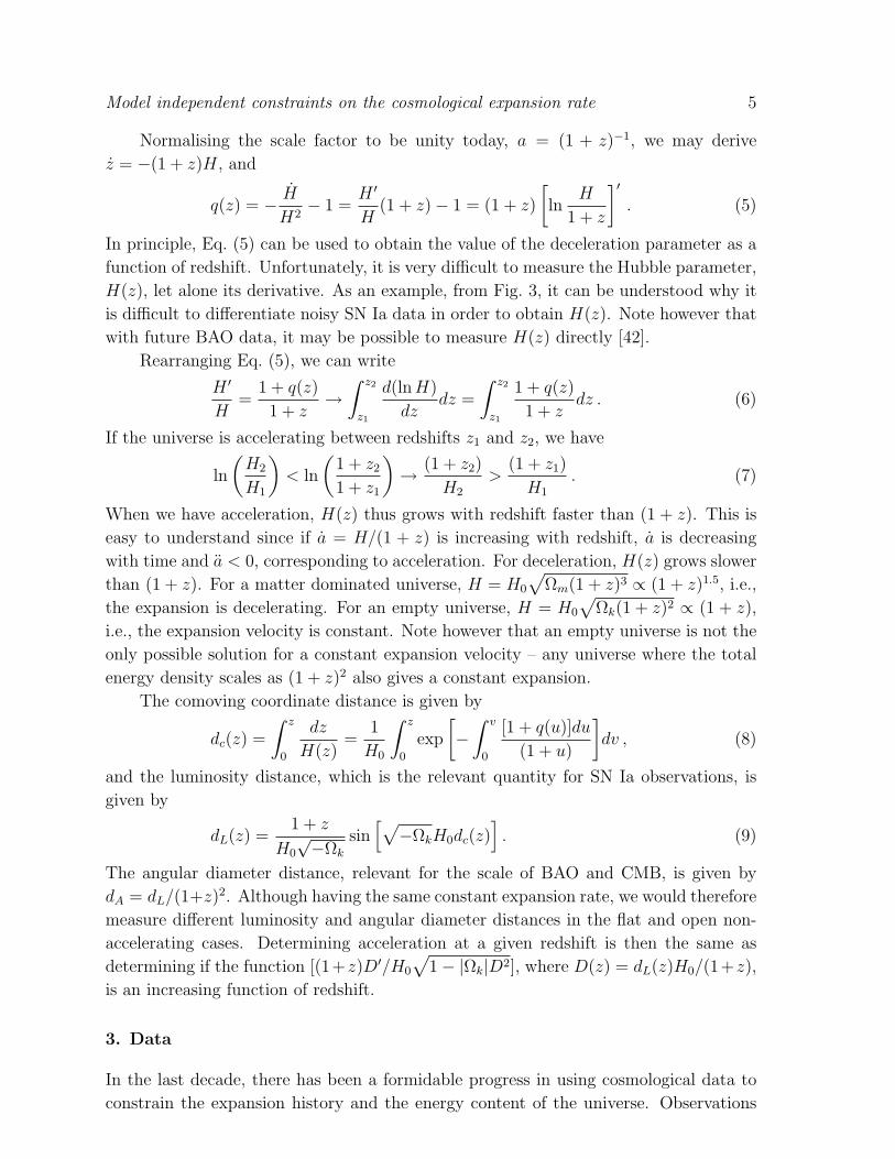
Figure 2. Best fit values of dA(z∗)/DV (z) at z = 0.2 (red) and z = 0.35 (blue),together with their 1σ errors, as measured from the scale imprinted in the CMB andBAO, shown in the parameter space for ΛCDM.

The constraints given by Eq. (13), individually place very weak constraints on

acceleration. Also, these constraints are highly degenerate with the curvature. In

Fig. 2, we show the CMB/BAO constraints in the Ωk − q0 parameter space for the

ΛCDM model, with their 1σ errors. It is clear that they require a large, negative,

deceleration parameter to be consistent with each other at 1σ CL, irrespective of the

curvature. Note also that a flat model is ruled out at this level. At 2σ CL however,

individual constraints on q0 and Ωk becomes very weak, and the combined constraints

are limited by the strong degeneracy exhibited between Ωk and q0. Nevertheless, the

data unambiguosly shows that Ωk > −0.1, i.e., the universe is not strongly overclosed.

4. Methods and results

In this section, we discuss how to determine the change of the expansion rate, or

q(z), without assuming a model for the energy content of the universe or a specific

gravitational theory. We are thus limited to using geometrical data as opposed to

methods that are sensitive to the growth of structure in the universe.

First, we discuss some difficulties that occur when trying to find q(z) by comparing

observed magnitudes of SNe Ia directly. This method has the advantage that it

can, in principle, detect a change in the expansion rate without somewhat ad-hoc

parameterisations of q(z). Some of these difficulties have been realised by Seikel and

Schwarz [41] – in particular the reliance on low redshift SNe Ia.

Alternatively we may parametrise the expansion with piecewise, constant

accelerations, i.e., we assume that q(z) can vary between redshift bins, but is constant

within the bins. This is the approach introduced by Turner and Riess [44]. We

investigate this further below, and find that it suffers from strong degeneracies with

curvature when including CMB data. We also investigate alternative parameterisations

of q(z), displaying the same degeneracies. However, we show that SN Ia data alone,


show that q(z = 0) < 0, irrespective of curvature.

We then present a method for determining acceleration, first employed in Riess

et al. [35], that relies on the fact that a−1 = (1+z)/H(z) is an increasing function when

the expansion is accelerating which seems to the case at low redshifts. However, since

the method relies on differentiating noisy SN Ia data, results at high redshifts have very

large uncertainties. Finally we present a new method which relies on a Taylor expansion

around an arbitrary ‘sliding’ redshift.

4.1. Inferring acceleration from m(z)

In SN Ia cosmology, the validity of a given cosmological model is tested by comparing

observed peak SN Ia magnitudes with the theoretical magnitudes for the given model,

m(z) = M + 5 log10

[dL(z)

1 Mpc

]+ 25 , (14)

where M is the absolute SN Ia magnitude. The normalisation of the magnitude

(containing, e.g., M and H0) is usually marginalised over, and constraints are derived

by examining the redshift evolution of the magnitudes.

Often, one presents SN Ia data in the form of the difference between the observed

peak magnitudes, and the theoretical magnitudes in an empty universe, me, where

the difference is normalised to be zero at low redshifts. Since an empty universe is

neither accelerating nor decelerating, it is sometimes claimed that one can infer the

state of the universal expansion from a quick visual inspection of this difference. One

common claim (at talks and discussions, if not in papers) is that negative values of

this difference, m−me < 0, shows that the universe is decelerating and positive values

that it is accelerating. Another inconsistent, but nevertheless common claim, is that

if the difference increases with redshift, the universal expansion is accelerating. If the

difference is decreasing, the expansion is decelerating. That is, the claim is that we can

infer the state of the expansion velocity by studying the sign of the derivative of the

difference with respect to redshift. Let us investigate these claims.

For the non-accelerating case, H ∝ (1 + z), and

dc,n =1

H0

ln (1 + z) , (15)

and

dL,n =1 + z

H0

√−Ωk

sin[√−Ωk ln (1 + z)

], (16)

where subscript n refers to non-accelerating expansion. For a flat, non-accelerating,

universe

dL,f =1 + z

H0

ln(1 + z) . (17)

For an empty, non-accelerating, universe, Ωk = 1, and

dL,e =1 + z

H0

(1 + z − 1

1 + z

)=z(z + 2)

H0

. (18)


For small curvature (Ωk 1), defining x =√−Ωkdc, we can use a Taylor expansion in

x and write

H0dL

1 + z=

1√−Ωk

sin (x) (19)

=1√−Ωk

(x− x3

6

)+O(x5) (20)

' H0

(dc +

Ωk

6d3

c

). (21)

The difference between the observed SN Ia magnitudes and those expected in a non-

accelerating universe is given by

∆m ≡ m−mn =5

ln 10ln

(dL

dL,n

). (22)

In Seikel and Schwarz [40], the inequality (valid in a flat universe)

dL(z) =(1 + z)

H0

∫ z

0

exp

[−∫ v

0

[1 + q(u)]du

(1 + u)

]dv (23)

<(1 + z)

H0

∫ z

0

dz

(1 + z)=

(1 + z)

H0

ln(1 + z) , (24)

was considered as evidence (∼ 5σ CL) for some period of acceleration up to redshift

z, i.e., q < 0 at some redshift. Allowing for spatial curvature, the evidence becomes

significantly weaker, or 1.8σ. We note [Eq. (18)], that this is equivalent to studying

the sign of ∆m, if the universe is flat. Assuming we can get rid of the dependence on

H0 and M by normalising the difference to be zero at low redshifts, we can study the

dependence of the curvature term by looking at the difference when subtracting empty

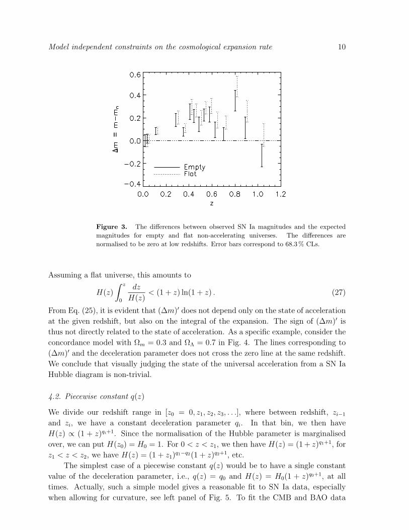
and flat non-accelerating cosmologies (Fig. 3). It is obvious that ∆m in fact is positive

for z ∼ 0.5, regardless of the curvature of the universe. A similar comparsion between

SNe Ia at low and mid/high redshifts was recently used in Seikel and Schwarz [41] to

provide a calibration-independent test of the accelerated expansion of the universe, the

conclusion being that the universe has accelerated at some epoch at ∼ 4σ CL. From

Eq. (23), it is evident that the sign of ∆m only tells us whether the integrated expansion

up to z is accelerating or decelerating on average, not the state of acceleration at a given

redshift.

We therefore turn to the second common claim, namely that if the difference ∆m

increases with redshift, the universe is accelerating at that very redshift. The derivative

of ∆m with respect to redshift is given by

(∆m)′ =5

ln 10

(d′LdL

−d′L,n

dL,n

). (25)

We note that (∆m)′ is independent of H0 and M . For (∆m)′ > 0, we have

d′LdL

>d′L,n

dL,n

. (26)


Figure 3. The differences between observed SN Ia magnitudes and the expectedmagnitudes for empty and flat non-accelerating universes. The differences arenormalised to be zero at low redshifts. Error bars correspond to 68.3 % CLs.

Assuming a flat universe, this amounts to

H(z)

∫ z

0

dz

H(z)< (1 + z) ln(1 + z) . (27)

From Eq. (25), it is evident that (∆m)′ does not depend only on the state of acceleration

at the given redshift, but also on the integral of the expansion. The sign of (∆m)′ is

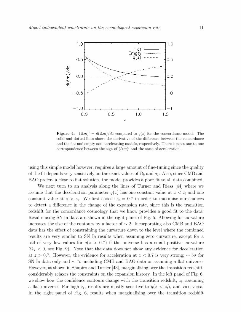
thus not directly related to the state of acceleration. As a specific example, consider the

concordance model with Ωm = 0.3 and ΩΛ = 0.7 in Fig. 4. The lines corresponding to

(∆m)′ and the deceleration parameter does not cross the zero line at the same redshift.

We conclude that visually judging the state of the universal acceleration from a SN Ia

Hubble diagram is non-trivial.

4.2. Piecewise constant q(z)

We divide our redshift range in [z0 = 0, z1, z2, z3, . . .], where between redshift, zi−1

and zi, we have a constant deceleration parameter qi. In that bin, we then have

H(z) ∝ (1 + z)qi+1. Since the normalisation of the Hubble parameter is marginalised

over, we can put H(z0) = H0 = 1. For 0 < z < z1, we then have H(z) = (1 + z)q1+1, for

z1 < z < z2, we have H(z) = (1 + z1)q1−q2(1 + z)q2+1, etc.

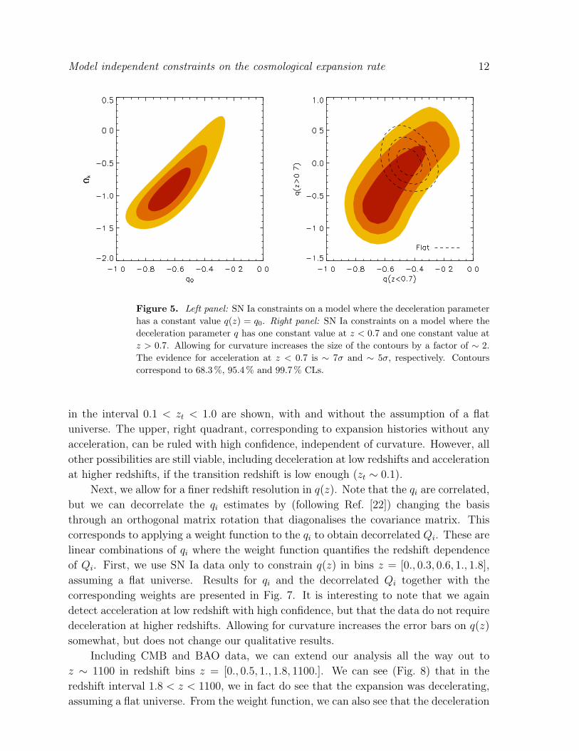
The simplest case of a piecewise constant q(z) would be to have a single constant

value of the deceleration parameter, i.e., q(z) = q0 and H(z) = H0(1 + z)q0+1, at all

times. Actually, such a simple model gives a reasonable fit to SN Ia data, especially

when allowing for curvature, see left panel of Fig. 5. To fit the CMB and BAO data


Figure 4. (∆m)′ = d(∆m)/dz compared to q(z) for the concordance model. Thesolid and dotted lines shows the derivative of the difference between the concordanceand the flat and empty non-accelerating models, respectively. There is not a one-to-onecorrespondence between the sign of (∆m)′ and the state of acceleration.

using this simple model however, requires a large amount of fine-tuning since the quality

of the fit depends very sensitively on the exact values of Ωk and q0. Also, since CMB and

BAO prefers a close to flat solution, the model provides a poor fit to all data combined.

We next turn to an analysis along the lines of Turner and Riess [44] where we

assume that the deceleration parameter q(z) has one constant value at z < zt and one

constant value at z > zt. We first choose zt = 0.7 in order to maximise our chances

to detect a difference in the change of the expansion rate, since this is the transition

redshift for the concordance cosmology that we know provides a good fit to the data.

Results using SN Ia data are shown in the right panel of Fig. 5. Allowing for curvature

increases the size of the contours by a factor of ∼ 2. Incorporating also CMB and BAO

data has the effect of constraining the curvature down to the level where the combined

results are very similar to SN Ia results when assuming zero curvature, except for a

tail of very low values for q(z > 0.7) if the universe has a small positive curvature

(Ωk < 0, see Fig. 9). Note that the data does not show any evidence for deceleration

at z > 0.7. However, the evidence for acceleration at z < 0.7 is very strong; ∼ 5σ for

SN Ia data only and ∼ 7σ including CMB and BAO data or assuming a flat universe.

However, as shown in Shapiro and Turner [43], marginalising over the transition redshift,

considerably relaxes the constraints on the expansion history. In the left panel of Fig. 6,

we show how the confidence contours change with the transition redshift, zt, assuming

a flat universe. For high zt, results are mostly sensitive to q(z < zt), and vice versa.

In the right panel of Fig. 6, results when marginalising over the transition redshift


Figure 5. Left panel: SN Ia constraints on a model where the deceleration parameterhas a constant value q(z) = q0. Right panel: SN Ia constraints on a model where thedeceleration parameter q has one constant value at z < 0.7 and one constant value atz > 0.7. Allowing for curvature increases the size of the contours by a factor of ∼ 2.The evidence for acceleration at z < 0.7 is ∼ 7σ and ∼ 5σ, respectively. Contourscorrespond to 68.3 %, 95.4 % and 99.7 % CLs.

in the interval 0.1 < zt < 1.0 are shown, with and without the assumption of a flat

universe. The upper, right quadrant, corresponding to expansion histories without any

acceleration, can be ruled with high confidence, independent of curvature. However, all

other possibilities are still viable, including deceleration at low redshifts and acceleration

at higher redshifts, if the transition redshift is low enough (zt ∼ 0.1).

Next, we allow for a finer redshift resolution in q(z). Note that the qi are correlated,

but we can decorrelate the qi estimates by (following Ref. [22]) changing the basis

through an orthogonal matrix rotation that diagonalises the covariance matrix. This

corresponds to applying a weight function to the qi to obtain decorrelated Qi. These are

linear combinations of qi where the weight function quantifies the redshift dependence

of Qi. First, we use SN Ia data only to constrain q(z) in bins z = [0., 0.3, 0.6, 1., 1.8],

assuming a flat universe. Results for qi and the decorrelated Qi together with the

corresponding weights are presented in Fig. 7. It is interesting to note that we again

detect acceleration at low redshift with high confidence, but that the data do not require

deceleration at higher redshifts. Allowing for curvature increases the error bars on q(z)

somewhat, but does not change our qualitative results.

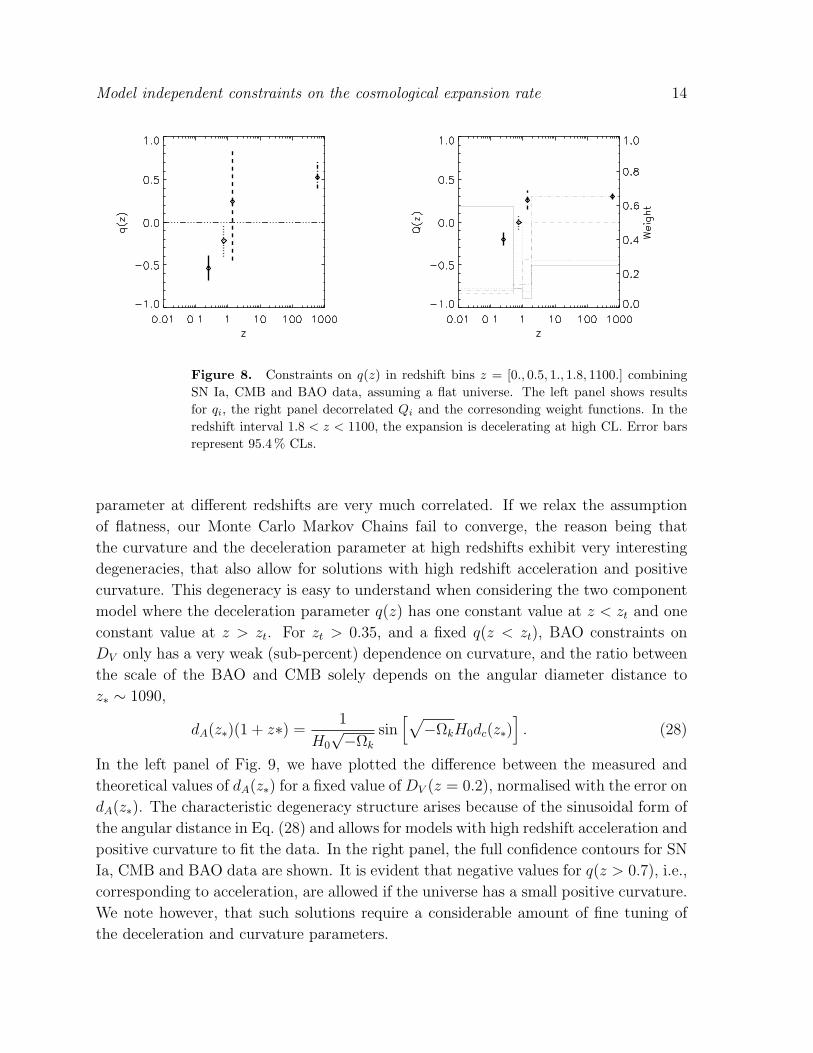
Including CMB and BAO data, we can extend our analysis all the way out to

z ∼ 1100 in redshift bins z = [0., 0.5, 1., 1.8, 1100.]. We can see (Fig. 8) that in the

redshift interval 1.8 < z < 1100, we in fact do see that the expansion was decelerating,

assuming a flat universe. From the weight function, we can also see that the deceleration


Figure 6. SN Ia constraints the deceleration parameter q when varying the transitionredshift zt. In the left panel, confidence contours for three discrete values of zt in a flatuniverse is shown. In the right panel, results when marginalising over the transitionredshift in the interval 0.1 < zt < 1.0 are shown, with and without the assumption ofa flat universe. Contours correspond to 68.3 %, 95.4 % and 99.7 % CLs.

Figure 7. SN Ia constraints on q(z) in bins z = [0., 0.3, 0.6, 1., 1.8], assuming aflat universe. The left panel shows results for qi, and the right panel decorrelated Qi

together with the corresponding weights. Error bars represent 95.4 % CLs.


Figure 8. Constraints on q(z) in redshift bins z = [0., 0.5, 1., 1.8, 1100.] combiningSN Ia, CMB and BAO data, assuming a flat universe. The left panel shows resultsfor qi, the right panel decorrelated Qi and the corresonding weight functions. In theredshift interval 1.8 < z < 1100, the expansion is decelerating at high CL. Error barsrepresent 95.4 % CLs.

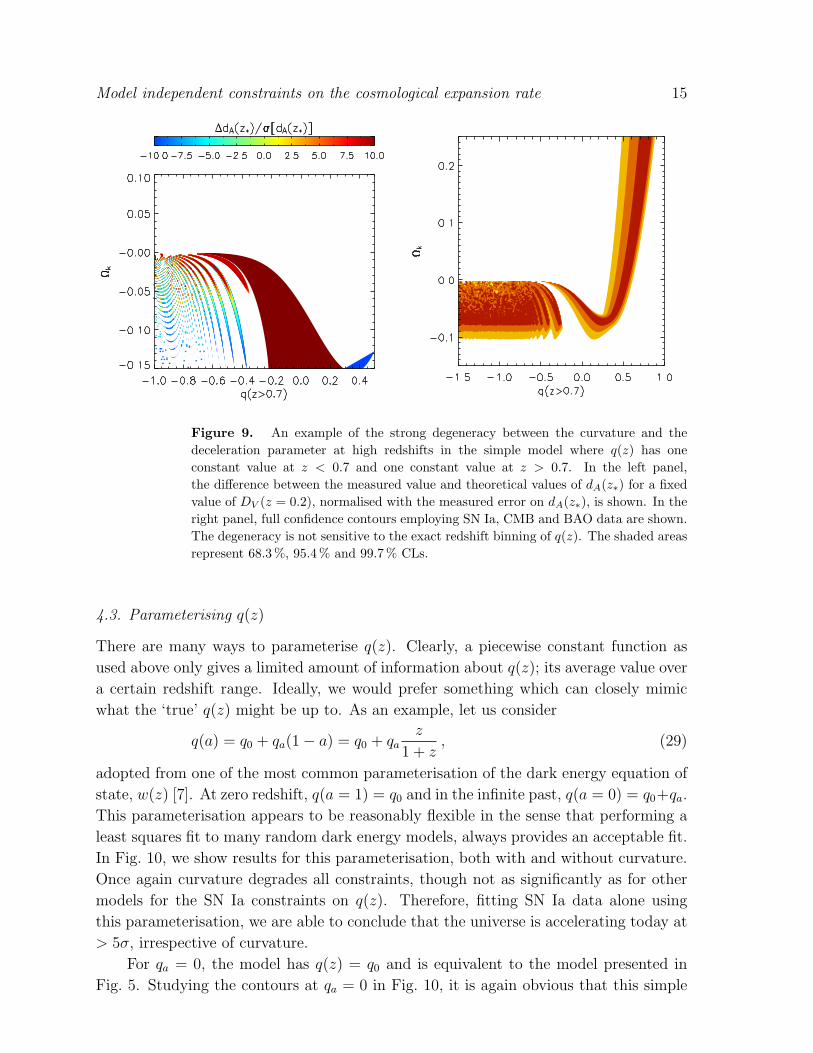
parameter at different redshifts are very much correlated. If we relax the assumption

of flatness, our Monte Carlo Markov Chains fail to converge, the reason being that

the curvature and the deceleration parameter at high redshifts exhibit very interesting

degeneracies, that also allow for solutions with high redshift acceleration and positive

curvature. This degeneracy is easy to understand when considering the two component

model where the deceleration parameter q(z) has one constant value at z < zt and one

constant value at z > zt. For zt > 0.35, and a fixed q(z < zt), BAO constraints on

DV only has a very weak (sub-percent) dependence on curvature, and the ratio between

the scale of the BAO and CMB solely depends on the angular diameter distance to

z∗ ∼ 1090,

dA(z∗)(1 + z∗) =1

H0

√−Ωk

sin[√−ΩkH0dc(z∗)

]. (28)

In the left panel of Fig. 9, we have plotted the difference between the measured and

theoretical values of dA(z∗) for a fixed value of DV (z = 0.2), normalised with the error on

dA(z∗). The characteristic degeneracy structure arises because of the sinusoidal form of

the angular distance in Eq. (28) and allows for models with high redshift acceleration and

positive curvature to fit the data. In the right panel, the full confidence contours for SN

Ia, CMB and BAO data are shown. It is evident that negative values for q(z > 0.7), i.e.,

corresponding to acceleration, are allowed if the universe has a small positive curvature.

We note however, that such solutions require a considerable amount of fine tuning of

the deceleration and curvature parameters.


Figure 9. An example of the strong degeneracy between the curvature and thedeceleration parameter at high redshifts in the simple model where q(z) has oneconstant value at z < 0.7 and one constant value at z > 0.7. In the left panel,the difference between the measured value and theoretical values of dA(z∗) for a fixedvalue of DV (z = 0.2), normalised with the measured error on dA(z∗), is shown. In theright panel, full confidence contours employing SN Ia, CMB and BAO data are shown.The degeneracy is not sensitive to the exact redshift binning of q(z). The shaded areasrepresent 68.3 %, 95.4 % and 99.7 % CLs.

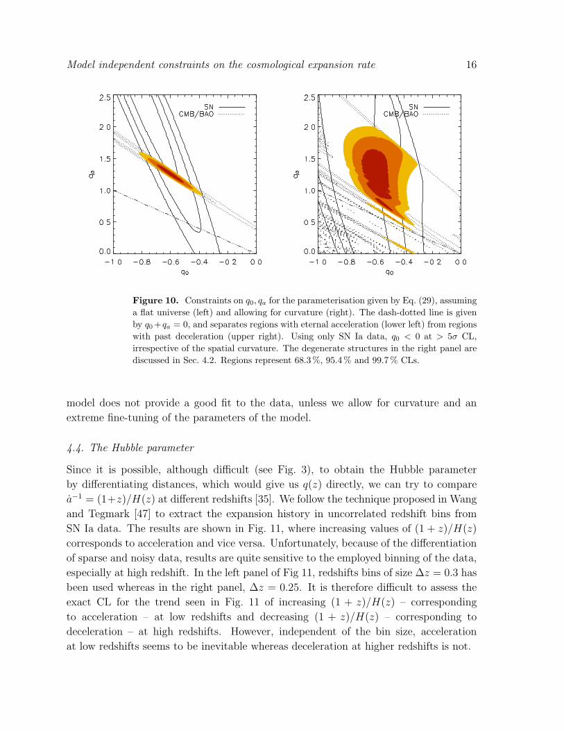
4.3. Parameterising q(z)

There are many ways to parameterise q(z). Clearly, a piecewise constant function as

used above only gives a limited amount of information about q(z); its average value over

a certain redshift range. Ideally, we would prefer something which can closely mimic

what the ‘true’ q(z) might be up to. As an example, let us consider

q(a) = q0 + qa(1− a) = q0 + qaz

1 + z, (29)

adopted from one of the most common parameterisation of the dark energy equation of

state, w(z) [7]. At zero redshift, q(a = 1) = q0 and in the infinite past, q(a = 0) = q0+qa.

This parameterisation appears to be reasonably flexible in the sense that performing a

least squares fit to many random dark energy models, always provides an acceptable fit.

In Fig. 10, we show results for this parameterisation, both with and without curvature.

Once again curvature degrades all constraints, though not as significantly as for other

models for the SN Ia constraints on q(z). Therefore, fitting SN Ia data alone using

this parameterisation, we are able to conclude that the universe is accelerating today at

> 5σ, irrespective of curvature.

For qa = 0, the model has q(z) = q0 and is equivalent to the model presented in

Fig. 5. Studying the contours at qa = 0 in Fig. 10, it is again obvious that this simple


Figure 10. Constraints on q0, qa for the parameterisation given by Eq. (29), assuminga flat universe (left) and allowing for curvature (right). The dash-dotted line is givenby q0 +qa = 0, and separates regions with eternal acceleration (lower left) from regionswith past deceleration (upper right). Using only SN Ia data, q0 < 0 at > 5σ CL,irrespective of the spatial curvature. The degenerate structures in the right panel arediscussed in Sec. 4.2. Regions represent 68.3 %, 95.4 % and 99.7 % CLs.

model does not provide a good fit to the data, unless we allow for curvature and an

extreme fine-tuning of the parameters of the model.

4.4. The Hubble parameter

Since it is possible, although difficult (see Fig. 3), to obtain the Hubble parameter

by differentiating distances, which would give us q(z) directly, we can try to compare

a−1 = (1+z)/H(z) at different redshifts [35]. We follow the technique proposed in Wang

and Tegmark [47] to extract the expansion history in uncorrelated redshift bins from

SN Ia data. The results are shown in Fig. 11, where increasing values of (1 + z)/H(z)

corresponds to acceleration and vice versa. Unfortunately, because of the differentiation

of sparse and noisy data, results are quite sensitive to the employed binning of the data,

especially at high redshift. In the left panel of Fig 11, redshifts bins of size ∆z = 0.3 has

been used whereas in the right panel, ∆z = 0.25. It is therefore difficult to assess the

exact CL for the trend seen in Fig. 11 of increasing (1 + z)/H(z) – corresponding

to acceleration – at low redshifts and decreasing (1 + z)/H(z) – corresponding to

deceleration – at high redshifts. However, independent of the bin size, acceleration

at low redshifts seems to be inevitable whereas deceleration at higher redshifts is not.


Figure 11. SN Ia constraints on a−1 = (1 + z)/H(z). Values increasing withredshift correspond to acceleration and vice versa. The dotted lines correspond to aflat universe with Ωm = 0.2 and Ωm = 0.4 from top to bottom. The normalisationis arbitrary and is set to agree at low redshifts. In the left panel of Fig 11, redshiftsbins of size ∆z = 0.3 has been used whereas in the right panel, ∆z = 0.25. Verticalerror bars correspond to 68.3 % CLs. Acceleration at low redshifts is clearly detectedwhereas deceleration at higher redshifts is not.

4.5. Sliding Taylor expansion

We can Taylor expand the scale factor around the current value according to

a(t) = a0 + a0(t− t0) +1

2a0(t− t0)2 +O(t− t0)3 (30)

= 1 +H0(t− t0)− 1

2q0H

20 (t− t0)2 +O(t− t0)3 . (31)

Since the comoving coordinate distance is given by

dc(t0) =

∫ t0

te

dt

a(t), (32)

we can write

dc(z) ' z

H0

[1− 1 + q0

2z

]. (33)

To first order, the distance is given by the expansion rate of the universe today, or

H0, and to second order by the change in the expansion rate today, or q0. We now

generalise Eq. (33) to allow for a Taylor expansion around any time, or equivalently,

redshift according to

a(t) ' a(t1) + a1(t− t1) +1

2a1(t− t1)2 (34)

= a1

[1 +H1(t− t1)− 1

2q1H

21 (t− t1)2

](35)

The comoving coordinate distance is given by

dc(t0) ' 1

a1

[(t0 − t1)− H1

2(t0 − t1)2 − (te − t1) +

H1

2(te − t1)2

], (36)


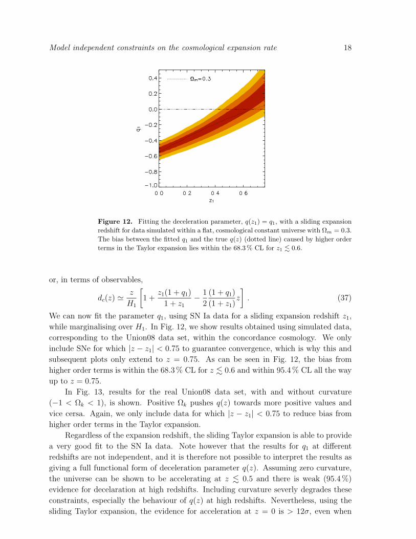
Figure 12. Fitting the deceleration parameter, q(z1) = q1, with a sliding expansionredshift for data simulated within a flat, cosmological constant universe with Ωm = 0.3.The bias between the fitted q1 and the true q(z) (dotted line) caused by higher orderterms in the Taylor expansion lies within the 68.3 % CL for z1 . 0.6.

or, in terms of observables,

dc(z) ' z

H1

[1 +

z1(1 + q1)

1 + z1

− 1

2

(1 + q1)

(1 + z1)z

]. (37)

We can now fit the parameter q1, using SN Ia data for a sliding expansion redshift z1,

while marginalising over H1. In Fig. 12, we show results obtained using simulated data,

corresponding to the Union08 data set, within the concordance cosmology. We only

include SNe for which |z − z1| < 0.75 to guarantee convergence, which is why this and

subsequent plots only extend to z = 0.75. As can be seen in Fig. 12, the bias from

higher order terms is within the 68.3 % CL for z . 0.6 and within 95.4 % CL all the way

up to z = 0.75.

In Fig. 13, results for the real Union08 data set, with and without curvature

(−1 < Ωk < 1), is shown. Positive Ωk pushes q(z) towards more positive values and

vice cersa. Again, we only include data for which |z − z1| < 0.75 to reduce bias from

higher order terms in the Taylor expansion.

Regardless of the expansion redshift, the sliding Taylor expansion is able to provide

a very good fit to the SN Ia data. Note however that the results for q1 at different

redshifts are not independent, and it is therefore not possible to interpret the results as

giving a full functional form of deceleration parameter q(z). Assuming zero curvature,

the universe can be shown to be accelerating at z . 0.5 and there is weak (95.4 %)

evidence for decelaration at high redshifts. Including curvature severly degrades these

constraints, especially the behaviour of q(z) at high redshifts. Nevertheless, using the

sliding Taylor expansion, the evidence for acceleration at z = 0 is > 12σ, even when


Figure 13. Fitting the deceleration parameter, q(z1) = q1, with a sliding expansionredshift. Note that constraints on q1 are significantly looser when allowing for curvature(in this case −1 < Ωk < 1). However, the evidence for acceleration at z = 0 is still> 12σ, including curvature. For a flat universe, q1(z1 = 0) < 0 at ∼ 15σ CL. Thelines correspond to the flat, cosmological constant universes with Ωm = 0.2 and 0.4,respectively. The shaded areas correspond to 68.3 %, 95.4 % and 99.7 % CLs.

allowing for curvature.

The reason for the closeness of the 2 and 3σ contours in the right panel, is that

at each redshift, the confidence contours in the [Ωk, q1]-plane has a banana like shape.

This has the effect that the resulting confidence levels for q1, which are obtained by

projecting the banana shaped contours on the q1-axis, has a non-gaussian shape.

5. Summary

In this paper, we have investigated to what extent we can measure the change in the

universal expansion rate, without making any assumptions about the energy content of

the universe. Consequently we are limited to geometrical data as opposed to methods

that are sensitive to the growth of structure in the universe. The data employed in this

paper includes the redshift-distance relation of Type Ia SNe, as well as the the ratio

of the scale of the baryon acoustic oscillations as imprinted in the cosmic microwave

background and in the large scale distribution of galaxies. We have used several different

methods to constrain the expansion history of the universe, all of which give the same

qualitative result.

From SN Ia data alone, it is evident that the universal expansion is accelerating at

low redshifts. In particular our new sliding expansion redshift method is able to detect

acceleration today at > 12σ, even allowing for curvature. Although there are hints from

SN Ia data that the universal expansion may have decelerated at high redshifts – as

REFERENCES 20

expected in the concordance cosmological model – we can only draw that conclusion with

high confidence if we also include CMB and BAO data, together with the assumption

of a flat or open universe. If the universe has a small positive curvature (Ωk < 0), it

is possible, although it requires a certain level of fine tuning, to accommodate the data

with acceleration also at high redshifts.

Acknowledgments

The authors would like to thank the anonymous referee for useful comments on the

paper. EM acknowledge support for this study by the Swedish Research Council and

SIDA. CC is funded by the NRF (South Africa). This was work initiated at a meeting

funded by the SASWE - Cosmology Bilateral agreement between South Africa and

Sweden.

References

[1] Astier, P., J. Guy, N. Regnault, et al., 2006, Astron. Astrophys., 447, 31

[2] Behrend, J., I. A. Brown, and G. Robbers, 2008, Journal of Cosmology and Astro-

Particle Physics, 1, 13

[3] Bolejko, K., in Golovin, A., G. Ivashchenko, and A. Simon, editors, 13th Young

Scientists’ Conference on Astronomy and Space Physics (2006)

[4] Bolejko, K. and J. S. B. Wyithe, 2008, ArXiv e-prints

[5] Buchert, T., 2008, General Relativity and Gravitation, 40, 467

[6] Caldwell, R. R. and A. Stebbins, 2008, Physical Review Letters, 100, 19, 191302

[7] Chevallier, M. and D. Polarski, 2001, International Journal of Modern Physics D,

10, 213

[8] Clarkson, C., B. Bassett, and T. H.-C. Lu, 2008, Physical Review Letters, 101, 1,

011301

[9] Clarkson, C., M. Cortes, and B. Bassett, 2007, Journal of Cosmology and Astro-

Particle Physics, 8, 11

[10] Clifton, T., P. G. Ferreira, and K. Land, 2008, ArXiv e-prints

[11] Cole, S., W. J. Percival, J. A. Peacock, et al., 2005, MNRAS, 362, 505

[12] Coley, A. A., 2007, ArXiv e-prints

[13] Copeland, E. J., M. Sami, and S. Tsujikawa, 2006, International Journal of Modern

Physics D, 15, 1753

[14] Daly, R. A., S. G. Djorgovski, K. A. Freeman, et al., 2008, Astrophys. J., 677, 1

[15] Davis, T. M., E. Mortsell, J. Sollerman, et al., 2007, Astrophys. J., 666, 716

[16] Eisenstein, D. J., I. Zehavi, D. W. Hogg, et al., 2005, Astrophys. J., 633, 560

[17] Elgarøy, Ø. and T. Multamaki, 2006, Journal of Cosmology and Astro-Particle

Physics, 9, 2

REFERENCES 21

[18] Garcia-Bellido, J. and T. Haugboelle, 2008, ArXiv e-prints

[19] Garcia-Bellido, J. and T. Haugbølle, 2008, Journal of Cosmology and Astro-Particle

Physics, 4, 3

[20] Garcıa-Bellido, J. and T. Haugbølle, 2008, Journal of Cosmology and Astro-Particle

Physics, 9, 16

[21] Hlozek, R., M. Cortes, C. Clarkson, and B. Bassett, 2008, General Relativity and

Gravitation, 40, 285

[22] Huterer, D. and A. Cooray, 2005, Physical Review D, 71, 2, 023506

[23] Jonsson, J., T. Dahlen, A. Goobar, et al., 2006, Astrophys. J., 639, 991

[24] Komatsu, E., J. Dunkley, M. R. Nolta, et al., 2008, ArXiv e-prints, 803

[25] Kowalski, M., D. Rubin, G. Aldering, et al., 2008, ArXiv e-prints, 804

[26] Larena, J., J.-. Alimi, T. Buchert, M. Kunz, and P.-S. Corasaniti, 2008, ArXiv

e-prints

[27] Li, N. and D. J. Schwarz, 2007, Physical Review D, 76, 8, 083011

[28] Li, N., M. Seikel, and D. J. Schwarz, 2008, ArXiv e-prints

[29] Percival, W. J., S. Cole, D. J. Eisenstein, et al., 2007, MNRAS, 381, 1053

[30] Perlmutter, S., G. Aldering, G. Goldhaber, et al., 1999, Astrophys. J., 517, 565

[31] Rapetti, D., S. W. Allen, M. A. Amin, and R. D. Blandford, 2007, MNRAS, 375,

1510

[32] Rasanen, S., 2008, Journal of Cosmology and Astro-Particle Physics, 4, 26

[33] Rasanen, S., 2008, ArXiv e-prints

[34] Riess, A. G., A. V. Filippenko, P. Challis, et al., 1998, Astron. J., 116, 1009

[35] Riess, A. G., L.-G. Strolger, S. Casertano, et al., 2007, Astrophys. J., 659, 98

[36] Riess, A. G., L.-G. Strolger, J. Tonry, et al., 2004, Astrophys. J., 607, 665

[37] Rosenthal, E. and E. E. Flanagan, 2008, ArXiv e-prints

[38] Sarkar, S., 2008, General Relativity and Gravitation, 40, 269

[39] Schmidt, B. P., N. B. Suntzeff, M. M. Phillips, et al., 1998, Astrophys. J., 507, 46

[40] Seikel, M. and D. J. Schwarz, 2008, Journal of Cosmology and Astro-Particle

Physics, 2, 7

[41] Seikel, M. and D. J. Schwarz, 2008, ArXiv e-prints

[42] Seo, H.-J. and D. J. Eisenstein, 2003, Astrophys. J., 598, 720

[43] Shapiro, C. and M. S. Turner, 2006, Astrophys. J., 649, 563

[44] Turner, M. S. and A. G. Riess, 2002, Astrophys. J., 569, 18

[45] Uzan, J.-P., C. Clarkson, and G. F. R. Ellis, 2008, Physical Review Letters, 100,

19, 191303

[46] Vanderveld, R. A., E. E. Flanagan, and I. Wasserman, 2008, Physical Review D,

78, 8, 083511

REFERENCES 22

[47] Wang, Y. and M. Tegmark, 2005, Physical Review D, 71, 10, 103513

[48] Zibin, J. P., 2008, Physical Review D, 78, 4, 043504

Documents

Model independent constraints on the cosmological ...redshift, considerably relaxed the constraints on the expansion history. Speci cally, using the so called \gold" dataset consisting