Model independent features of the two-particle correlation function

APH N.S., Heavy Ion Physics 1 (1995) 1-31 HEAVY ION PHYSICS �9 Akad› Ktad£

Model Independent Features of the Two-Particle Correlation Function

Scott Chapman, Pierre Scotto and Ulrich Heinz

Institut fª Theoretische Physik, Universit~it Regensburg D-93040 Regensburg, Germany

Received 15 September 1994; final revised version 17 February 1995

Abstraer. The Hanbury-Brown Twiss correlation function for two identical particles is studied for systems with cylindrical symmetry. Its shape for small values of the relative momentum is derived in a model independent way. In addition to the usual quadratic "side", "out" and "longitudinal" terms in the exponent of the correlator, a previously neglected "out-longitudinal" cross term is found and discussed. The model- independent expressions for the size parameters of the HBT correlation function are interpreted as lengths of homogeneity of the source, in distinction to its purely geometrical size. They are evaluated analytically and numerically for two specific thermal models featuring collective transverse and longitudinal flow. The analytic expressions derived allow one to establish qualitatively important connections between the space-time features of the source and the shape of the correlation function. New ways of parametrizing the correlation function anda new approach to the measurement of the duration of the emission process are suggested.

1. lntroduction

It is widely accepted that if the nuclear matter created in ultra-relativistic heavy-ion collisions attains a high enough energy density, it will undergo a phase transition into a quark- gluon plasma. For this reason, it is of great interest to determine the energy densities actually attained in these collisions. The total interaction energy of a given reaction can be directly measured by particle calorimeters and spectrometers. Although there is no analo- gous direct measurement for the size of the reaction region, Hanbury-Brown Twiss (HBT) interferometry [I] provides an indirect measurement for both the spatial and temporal extent of the reaction region in terms of the correlations between produced particles.

Consequently, the greatest challenge for theorists studying HBT interferometry to- day is to determine exactly what information the reported expe¡ correlation radii are telling us about the source. Obviously, the most powerful statements to this effect are those which can be made in a model-independent fashion. Although the individual reac-

0231-4428/95/$ 4.00 �9 1995 Akad› Kiad£ Budapest

2 Scott Chapman, Pierre Scotto and Ulrich Heinz

tions measured experimentally may not be completely cylindrically symmetric, it is safe to assume that a large ensemble of similar reactions will produce cylindrically symmetric data. For this reason, we have generalized the work of [2] by using the covariant Wigner function formulation [2-6] of HBT interferometry to derive cylindrically symmetric, but otherwise model independent expressions for the correlation radii, both using standard cartesian momentum differences and boost-invariant rapidity differences. Two important model-independent statements can then be made. First, cylindrical symmetry in no way precludes the existence of an "out-longitudinal" cross term in the correlation function [7], and in fact in general such a term would be expected to appear. Second, the correlation radii do not necessarily measure the geometrical size of the reaction region, but rather the lengths of homogeneity of the source as seen by a particle emitted with the average momentum of the studied pair [8].

To see how these effects manifest themseives in a concrete (though still qualitative) way, we apply our model-independent formalism to two specific thermal models, both of which feature a constant freezeout temperature. The first model is a generalization of [9], featuring nonrelativistic hydrodynamic flow which, however, can be different in the longitudinal and the transversal directions. Since this model is completely gaussian, it is easy to verify explicitly that the spatial lengths of homogeneity depend not only on the geometrical size of the reaction region, but also on the spatial gradients of the hydrodynamic flow. Similarly, the cross term just measures the temporal length of homogeneity, which in this nonrelativistic case is simply the duration of particle emission.

The second model that we consider is a variation of [10], featuring a Bjorken scaling longitudinal flow anda nonrelativistic transverse flow. Although this model is not completely gaussian, analytic results derived from a modified saddle point approximation are able to reproduce numerically generated results to within 20-30% for pions and much better for kaons. The analytic results provide valuable qualitative insights into the generic influence of various physically relevant parameters of the source distribution on the shape of the correlation function. We show that this model features a large cross term whose effects can clearly be seen in a two-dimensional plot of the "out-longitudinal" correlation function. In addition, we show that the theoretical interpretation of the correlation radii simplifies immensely when rapidity differences rather than longitudinal momentum differences are used to parametrize the correlation functions. In light of these results, we make explicit suggestions of useful new ways in which experimentalists can organize their measured correlation data.

2. Model lndependent Correlation Radii

The HBT correlation function for two identical on-shell particles is given by [ 1,11 ]

�9 2 P2(Pl,P2)

C(PI'P2) N2-N PI(PI ) PI(P2 ) ' (1)

where P , ( p ) = E (dN/d3p)is the invariant l-particle distribution for a particle with L p

mass m and 3-momentum p, P2 is the corresponding invariant 2-particle distribution func-

Model Independent Features of the Two-Particle Correlation Function 3

tion, and N (N 2) is the average number of particles (squared) produced in a reaction. By quite general arguments it can be shown that in the plane wave approximation for chaotic sources [2-6]

C(P l ,p2 ) 1 + ~ d4x S x ,~(pl +p 2) eiq "x -- , ( 2 )

P I ( P 1) P I (P2)

where the + (-) sign is for bosons (fermions), q = PI - P2 is the 4-momentum difference of the two particles, and pO = Ei are the on-shell energies. Furthermore, the emission function S(x,p) is a scalar function of the 4-vectors x and p which obeys

~d4x S(x, pi ) = P i (p / ) . (3)

As an example, in the local hydrodynamic formulation involving a sharp 3-dimensional freeze-out hypersurface one has [12]

S(x,p) = 1 p . n (x) (4) (2~) 3 exp [~(x)(p �9 u (x) -/ . t (x))] -TI '

where u~t(x), ~(x), ~t(x) and

ntl(x ) = [xd3o'!a (x ' ) ~ (4)(X-X') (5)

denote the local hydrodynamic flow velocity, inverse temperature, chemical potential, and normal-pointing freeze-out hypersurface element, respectively.

2.1. Cartesian Momentum Coordinates

In order to simplify computation, the correlation function is often approximated by using on-shell momenta in the emission function [2,4,12,13]. For example, one can define [4]

Sd4x S(x, K) eiq "x 2 C(Pl ,P2)-~ C'(q, K) = 1 +-- (6)

Sd4x S(x,K)I 2 '

1 where K = ~ (p i + P2) and K o = E K = [ m2 + I KI2] ~/2 Neither the present definition of K nor the different definition we will use in the next subsection should be confused with the usual off-shell definition of K 0 = 1 (El+E2) which is suggested by Eq. (2).

We begin by using the conventional HBT cartesian coordinate system which is defined as follows: The "longitudinal" or ~ (subscript L) direction is defined to be parallel to the beam; the "out" or .~ (subscript _1_ ) direction is parallel to the component of K which is perpendicular to the beam; and the "side" or ~ (subscript s) direction is the remaining transverse direction. For ]q[/E K << 1, we then have

q . x = 13. q t - q_l_p cos~b - qsp sin~b - qL z , (7)


where p = [x 2 + y2]V2, r = tan-l(y/x) and I~ = K/E K is the velocity of a particle with momentum K.

To present their data, expe¡ use these coordinates in one of two different reference frames, both of which can be obtained by a longitudinal boost from the lab frame: The fixed observer frame is usually taken as the rest frame of the participant center of mass and is the same for all particle pairs [14-16]. The "LCMS" (longitudinally co- moving system) frame, on the other hand, is defined as the frame in which K L = 0 and thus varies for pairs with different longitudinal momentum in the fixed observer frame [16- 18]. Consequently, as pointed out in [9,10,18] a qL-correlation function should then only be measured at a given value of K L, and an averaging over K L should be avoided. How- ever, since different values of the longitudinal component of the mean momentum lead to different reference frames, the interpretation of a possible KL-dependence of the correlation radii turns out to be conceptually nontrivial in the LCMS. Later, however, we will show that for the special case of a system which is undergoing Bjorken longitudinal expansion, the LCMS radii are nothing more than approximations of fixed frame radii which are evaluated in rapidity coordinates (see next subsection). To avoid the complication of shifting reference frames, we perform aU of our calculations in a fixed frame, though we do point out how to find the LCMS results.

Due to the symmetry C(pt, P2) = C(p2, Pt) and the fact that when q --~ 0 the correlation function C(pl,P2) ~ 1 _+ 1 (as can be seen from Eq. (2)), it is reasonable to assume that for sufficiently small momentum differences q, C takes the form

C(Pl , p2 ) = l + e x p [ - ~ q (8) �9 i# j

where the coefficients R 2 and R2.; depend " 1 on the average palr momentum K = ~ (p 1 + 112). I I i .

2 v Note that the R 2 are always poslttve, but the R.. can be either positi e or negative; we simply use the R z. notation to denote the fact that they are coefficients of terms which are

tJ quadratic in qi. Furthermore, in order for the peak of the correlation functson to be located at q = 0, it must be true that for all i and j

ZIRol 2 < R 2 i + R 2 . 1 (9)

- ,, 2 w 1 t x ss ns for the radn R and R 2 Below e obtain model "ndependen e pre lo "" i ii by effectively taking second derivatives of the correlation function with respect to qi and qj around q = 0.

Before proceeding, we would like to point out that one must take care when comparing the above radii to experimentally measured correlation radii since the former measure second derivatives of the correlation function around q = 0, while the latter are parameters of a gaussian fit to the whole correlation function [ 14-17] and are essentially determined by its width. Nevertheless, there are many interesting "gaussian" models for which the two different ways of defining the radii give roughly the same results. To the extent that the part of the correlation function measured by experimentalists is roughly gaussian, cer- tain of these "gaussian" models should be able to provide good descriptions of the data. In this work we are therefore restricting the application of our model independent results to "gaussian" models for which the simple expressions that we generate below provide valu-


able insights as to how various parameters of a given source distribution will qualitatively affect measurable features of the correlation function.

Since S(x,p) transforms asa scalar under Lorentz transformations, it can be taken to have the following functional form

S(x,p) = S(x,p . p , p . u ( x ) , p , v ( x ) , p , w(x ) .... ), (10)

where u, v, w, etc. are space-titne dependent local 4-vectors. Cylindrical symmetry can be enforced by demanding that S has no explicit ~p dependence and that all of the relevant local 4-vectors be cylindrically symmetric. For example,

u(x) = (u 0, upcos~, upsin~, Uz), (11)

where u 0, Up and u z are all independent of dp. Given these definitions,

K. u = EKU O -K_l_u9 cos0 ? -KLU z , (12)

so for cylindrically symmetric systems S(x, K) is even in ~. Using (7), we can now expand the factor exp(iq.x) in Eq. (6) for small q, keeping

only the terms even in ~, because the odd terms vanish upon t~ integration. We find

C(q, K) = 1 + { 1 _q2(y2)_( [q.l. ( x - p_l_t) + qL ( z - ~L t) ] 2) (13)

+(q• ( x - ~ • + qL ( Z - ~ L t) )2 + O[( (q" x) 4)]},

where x = pcos~, y = psinO, and we have introduced the notation

(~) = 1 I d 4 x ~ S ( x , K ) . (14) PI(K)

Eq. (13) generalizes similar results obtained in [2] for a 1-dimensional situation. Exponen- tiating (13), we can see that for any cylindrically symmetric system the correlation function for small momentum differences will take the form

2 2 2 2 2 2 6"(q, K ) = 1 + e x p [ - q s R s - q • 1 7 7 L - 2q• (15)

The R/2 which correspond to the approximation (6) can simply be read off as the coefficients of the corresponding qiqj terms in Eq. (13):

R 2 = (y2)

R 2 = ( ( x - ~ • 2 ) - ( x - ~ & t ) 2,

R 2 = ((z - ~L t) 2) _ (Z - ~Lt) 2, (16)

R2 L = ( ( x - ~J• (Z - ~Lt)) - ( x - ~• - ~Lt).

They are functions of K due to the K-dependence of S(x, K) in definition (14) of the expec- tation value ( . . . ) . One of the most interesting features of (15) is, as pointed out in [7], the occurrence of a q• cross term which has never before been discussed in the literature.

Before exploring the implications of this term, we would like to give an intuitive interpretation of the model-independent expressions (16). To this end we follow the work of


[8] and introduce the concept of a length of homogeneity. We begin by defining the space- time saddle point ~ of the emission function S(x,K) through the four equations

d dx~tlnS(x, K) I~ = 0, (17)

where ~ = { 0,1,2,3 }. Essentially the saddle point is that point in space-time which has the maximum probability of emitting a particle with momentum K. A saddle point approximation for S(x, K) can then be made in the following way

[~ s(x, K)~_s(;c, K)exp - (x2~~~t) 2

. - ~ , B , v ( x ~ , - ; c , ) ( X v - ;Cv , [.t>v

(18)

where we define the length of homogeneity of the source in the ~th direction by

= d 2 . J- l /2 [---2Tln S (x, K)

~~t(K) L dxll l-

and

d_ d__ lnS(x, bol;. BI~v(K) = ax~tax v

(19)

(20)

From (19), it can be seen that the length of homogeneity provides a measure of the region over which the source is relatively constant as seen by a particle with momentum K. Obvi- ously, if a source has large temperature or flow gradients, the length of homogeneity may be determined by these more than by geometrical density gradients.

Notice that if Brtv<< 1/~2 (which can always be arranged by making the right choice of variables), then

( x ~ ) - ( x . ) 2 = ~~, (21)

where we do not use the summation convention. Since all of the radii of Eq. (16) contain terms of the above form, these radii are evidently measuring lengths of homogeneity rather than strictly geometrical sizes. For example, the "side" radius measures 9~2 (in the

direction), which by cylindrical symmetry must be equal to the length of homogeneity in the transverse or radial direction. Later, we will see how these lengths manifest them- selves in definite models.

Corrections to the radii of (16) can be calculated by considering the exact correlation function (2) rather than the approximation (6). (Within their one-dimensional model these corrections were also found in [2].) The corrections to the denominator can be found by noticing that due to cylindrical symmetry, PI(P) is really only a function of the longitudinal and radial components ofp. Hence,


, , q2 O(Iq[ 3/E2) = PI KL+~qL, K_L+~q_L+'ff~-I+

Keeping only up to quadratic corrections in q,

[ 1( q.2 ~ d qL d a(q_l_ d qL d ]2 l P1(Pl) -~ 1 + ~~q_L + ~--~&)~-~& + T ~ ~ L + ~[ T~-~--~& + T~~--~L) _]PI(K) - (23)

PI(P2) can be found simply by letting q---) - q in the above expression. Combining these, re-exponentiating, and again keeping only terms up to second order in qi, we get

"~ -q28R2-q2 8R2-q2L~)R 2- 2q~q 8R2.1, PI(PI)PI(P2 ) [PI (K)] 2exp [ , . _I_ .I_ L ~ L ~ ~ . (24)

where

~R 2 _ 1 d lnPl(K) I/r s 4K.LdK_L

1 d 2 ~R2 - 4dKŸ InPI(K)IKt;

8R 2 - 1 d 2 4dK 2 InPt(K) [g• ;

8R2LL -- 4dKL lnP l ( K ) I r L rA.

(25)

Notice that all of these corrections are direct experimental observables. For example, ~SR 2 is the curvature of a plot of In PI(P) asa function of P_l. for fixed PL"

Finally, we turn to the corrections induced by using the correct off-shell energy 2-1 (pO + pO) in the emission function of Eq. (2) rather than the approximate on-shell value E K of Eq. (6). Again making a Taylor expansion for lql << E x,

,o [ , ] 2(Pl +pO)~_ EK ] +8_.~K(lq12 ( l i . q )2 )

I ~- [m2+lKI2+~( lq l 2 - (IB' q)2)],

(26)

we can see that

Therefore, we can expand around the on-shell momentum K in the following way:


To quadratic order in q, then

exp Ilt]q/2- (13. q)2)d-~lnPl(K)l~d4xS(x , K)e iq'x.

(28)

(29)

Putting everything together, we find the following corrected model-independent expressions for the correlation radii of Eq. (15):

( 1 d 1 d ] InP,(K); R2 = (y2) + 4K.I.dK,I, 2dmZ) ,

R Ÿ = ((x - ~,• 2) _ ( x - J],• 2

+ ~4dK 2 - I],• ~ lnPI(K) ;

R 2 = ((z - I]Lt) 2) - (Z - ~Lt) 2 (30)

+ ~ 4dK 2 2

R 2 L ~- ( ( x - ~• - ~Lt)) - ( x - ~,i,t)(z - ~L t)

+(1 d 2 , ~ ~,• lnP, (K) ~ ~ ~~~,~

Note that LCMS radii can be found from the above expressions simply by setting ~L = 0. The first thing to observe about the above radii is that cylindrical symmetry alone

does not cause R~_ L to vanish, so a q• cross term (as in (15)) should be included in any experimental fit to the data. However, itis interesting to note that for the case K• = 0 (~,• 0), S(x, K) is independent of r so RŸ does vanish (see Appendix). Furthermore for this case R~ = R 2 as it must, since if K• = 0 it is impossible to define a difference between the "out" and "side" directions. This means that the q• cross term (as well as the difference between RŸ and R. 2 ) will be most noticeable for pairs with large K• We would also like to point out that the cross term vanishes for spherically symmetric systems ifone redefines the ~ direction in the direction of K [9], since in this case K• =0 by definition. For any collision experiment, however, it is best not to make this redelŸ since only cylindrical symmetry about the beam can be assumed. It should also be noted that if future heavy ion experiments are able to generate HBT correlation functions from a single event, then cross terms involving qsq• and qsqL should be included in any fits as tests of the cylindrical symmetry of the individual reaction under consideration.


Before going on, we would like to say a few words about the validity of the approximation of Eq. (6) and the size of the correction terms. Since the 8R 2 of (25) can be measured from single particle distributions, a model-independent experimental estimate can be made as to the accuracy of the approximation of (6) by comparing those correction terms with the H B T radii found by fitting correlation data with gaussians as in (15). I f the former are much smaller than the latter, then (6) should be a good approximation. For example, the slopes and curvatures seen in heavy ion collision data generate 8R 2 which typically have scales on the order of

8R 2 < 1 4 ( 150 MeV) 2' (31)

whereas R 2 R 2 and R 2 typically have scales on the order of R 2 - 1 / ( 7 5 M e V ) 2 [14] so the approximations to these radii from Eq. (6) should be good to within roughly 5 %. As we will see later, however, the corrections could become important when determining the magnitude (and sign) of the cross term or the difference between R Ÿ and R2s for systems with very short emission times.

2.2. Boost Invariant Coordinates

Now we would iike to rederive the results of the preceding section using rapidities rather than longitudinal momenta, since the former boost invariant variables are usually more appropriate for relativistic collision experiments. Returning to Eq. (6), let us make an alternative on-shell definition of the 4-vector K:

K = (mtchY, K t, mtshY) , (32)

l 2 2 1 1 where K t = ~ (P l t + P2/) ' m2 = m + ii~,l, I, = ~ (y l + y2), and Yi = ~ln[(Ei +piL ) / (E i -piL)]. Note that we use the subsc¡ t throughout to denote transverse 2-vectors as well a s m t and other general transverse quantities; this should not be confused with the subscript _L which we use only to denote the "out" direction.

Jus tas in the last subsection, we can expand the factor exp ( i q . x) in Eq. (6) for small momentum (and rapidity) differences. This time we find:

(7(y, qs' q• Y' K • 1 + { 1 _ q.2<y2)

- ( [q• ( x - (K_l_/mt)'cch O] - Y) ) + Y m t ' ~ s h 0 ] - Y ) ] 2 ) (33)

+(q• (x - (K• xch (TI - Y) ) + ym/csh (11 - y ) ) 2 } ,

= t In [(t+z)/(t-z)] is the where Y=Yl-Y2, "~=[t2-z2] v, is longitudinal proper time, and ti space-time rapidity. (The reader should take care not to confuse the rapidity difference y with the cartesian coordinate y.) This time after exponentiating, we get a correlation function of the form:

(?(Y' qs' q• Y' K• = 1 _+ exp [ - "ls"2R2s - "1&--_1_"2 ~,2 _ y2cx2 _ 2q •177 , (34)


where again for the approximation of Eq. (6) the correlation "radii" can be read off as the coefficients of the appropriate terms in Eq. (34):

R 2 = <y2), S

R 2 = < [x - (K_l_/mt)'~ch(" q - y)]2>

- ( x - (K_L/mt) "~ch (I] - y))2, (35)

a 2 = ( [m/1:sh (1] - )I) ] 2) _ (mtzsh (1] _ }i))2,

R_Ly = ( [mtx- K_L'CCh (~ q - Y)]'csh(1] - Y))

- (mtx - K_l_'~ch (r I - Y) ) ('l;sh (r I - Y) ).

Similarly to Eq. (24), quadratic corrections which arise from expanding the denominator of (2) for small q can be found to give

Pl(Pi)fd4x S(x, P1 (p2)2 = K ) exp(-q '2~R'2-qŸ176 2q-l-Y £

~iR2 _ 11 d lnPl (K) ] , s 4 K.j_ d K_L Y

8R 2 = 1 d 2 -4dK-----~~ lnPl (K) q ,

~0~2 - 1 d 2 4dy2 In PI (K) [K• '

~R_L y - ~d~{d'~'-&lnPl(K) lY} K•

where

(36)

(37)

Note that these "side" and "out" corrections take the same formas those in Eq. (25), except that here rapidity rather than longitudinal momentum is held fixed while taking the derivative with respect to K_L. Since experimental one particle spectra are usually presented as functions of rapidity and not longitudinal momentum, these corrections can be even more readily measured from the data than those of the previous subsection.

Finally, we turn again to the corrections induced by using the exact off-shell 4-vector ~ (PI +P2) in the emission function of Eq. (2) rather than the approximate on-shell 4- vector K of Eq. (32). Making a Taylor expansion for small y and qt, we find

1 2 ( KŸ 1 2 1 2 2 r,L~ (P, + p2)j2-I ~_ m2 + 7~ql ~ 1 - ;'m"'; ) [ + 7~qs + 7,Y mt . (38)


Furthermore, if we reparametrize the local 4-vectors of (10) in the following way

u (x) = (utch ~, upcosd~, up sinO, utsh~), (39)

where u t, up and ~ are independent of ~, then

1 1 2 ( K2") 1~2--1. 2 _ 2 J 1/2 ~(p,+p2).z,~-Em2,+aq• 1-m-~-TJ+4qs-'-71 y " ' t u,ch(Y-~)-K_LUpCOS�91 p. (40)

Therefore, to quadratic order in y and qt

Id4xSIx '~(Pl+P2)]eiq 'x { ~ I ( KŸ ] d ~ l n P l ( K ) l = exp q2 1 _ _ _ + q 2 + y 2 m 2 .(41) Id4xS(x, K) e iq'x m2 " dmZ J

The most interesting thing to note about this off-shell correction is that it has no effect on the coefficient of the q.LY cross term.

Putting everything together, we find the following corrected model-independent expressions for the correlation radii of Eq. (36):

1 d )lnP,(K) 1 d R 2 ~ (y2) + ,4K-LdK_L 2dmZ)

RI'" ( [x - (K_L/m t) "~ch (11 - Y) ] 2} _ ( x - (K_L/m t) "cch (11 - I0) 2

~.4dK-~~ ~(1 ~2t2/~m2/ lnPl(K) ,

~2 _ ( [tot,es h (q _ Ii) ] 2) _ (mtzsh (11 _ y) )2 (42)

1 2 d (1 d 2 ~m, ~m2) lnPl (K) +,.aaT~ R_Ly ~-- ( [mtx- K_LZCh (11 - Y) ] xsh (11 - Y))

- ( m t x - K_LZCh ('11- Y))(zsh (11 - Y)) + - - - - - l d d 4dYdKLlnPl(K) �9

Again, although R_Ly does not vanish in general, it does vanish for pairs with K_L = 0 (see Appendix).

3. A Model with Nonrelativistic Expansion

To get an idea of the usefulness of the model independent expressions just derived, we study a slight generalization of the thermal emission function presented in [9]:

S(x ,K) = (2~) EK 3 e x p ( K ' u ( x ) ) . (43)


Here T is a constant freeze-out temperature, and we define the space-time distribution of the source by a product of gaussians in the center of mass frame of an expanding fireball

1 [ ( t - / o )2 p2 Z2L2 ] H ( t ) l ( p ) J ( z ) = [ 2 ~ ( & ) 2 ] l q - 2~~i-~~- 2R 2 . (44)

For the thermal smea¡ factor in Eq. (43), we take a nonrelativistic linear expansion 4- velocity

u (x) = [1 - (VRP/RG) 2_ (ULZ/LG) 2] -1/2 ( 1, VRX/RG ' VRY/RG, ULZ/LG )

~ 1 + ~~ ( vRp /RG) 2 + ~1 (VLZ/LG) 2, VRX/RG ' VeY/RG, vLZ/LG ,

where v R y 1 and v L y ! are the transverse and longitudinal flow velocities of the fluid at p = R a and z = L a, respectively.

Note that in the limit & --~ O, S(x,K) becomes the Boltzmann approximation to the hydrodynamic emission function of Eq. (4) with a constant freeze-out time t o and a local chemical potential given by:

t.t(x) p 2 Z 2 - ( 4 6 )

T 2=�91 2L~

In a sense, use of a nonzero St can be thought of as a smearing of the sharp 3-dimensional freeze-out hypersurface t = t o over the fourth (temporal) dimension.

Since the model is completely gaussian, analytic calculation of the one-particle dis-

/72.2/,-2 2 2 2 �9 **VR~.l -

2R2 T 2 + 2 L 2 T 2 ) ,

tribution is straightforward, yielding

EK 2 ( Etc PI(K) = . , ~R ,L , e x p | - --~ +

(2=) ~ [ *'

~~ 4 1 - - + T'~J

where

(47)

(48)

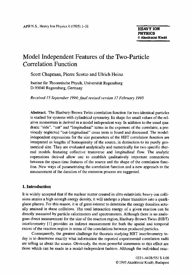
In Fig. 1 we plot P I (K) a s a function o f m t - m for midrapidity (Y= 0) particles from a source with the parameters R G = L G = 3fm, T = 150MeV, and v L = 0. The decrease in the slope of the pion curves when the transverse flow is changed from v R = 0 to v R = 0.5c can be understood in terms of an effective blueshifted temperature [ 19]

= T [ 1 +VR]ll2 Teff L 1---~R I (49)

From Eq. (48) it can also be seen that asymptotically as K L ~ o o


R2aT R2, - ~ - - (50)

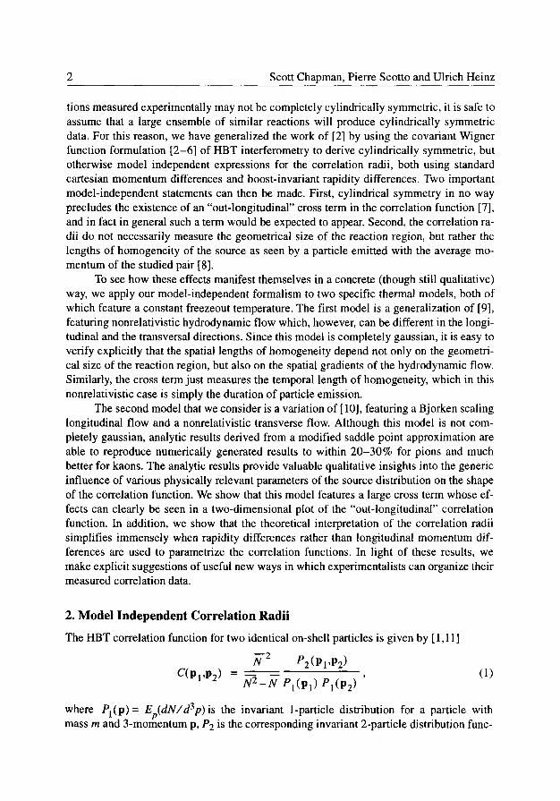
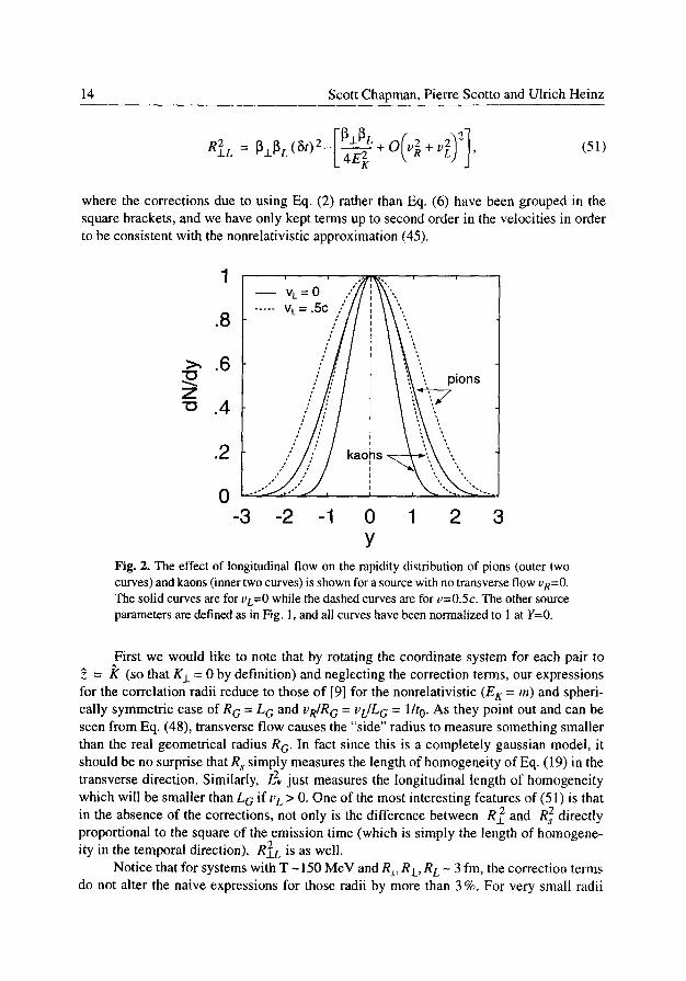
so that for pL= 0 the K_L dependence of the prefactor drops out and the spectrum takes the form of a pure exponential with an inverse slope of Tel f = 2 T. Figure 1 also features a kaon distribution with flow which shows the same behavior. As can be seen from Fig. 2, increasing the amount of longitudinal flow from v L = 0 to V L = 0.5C causes a widening of the rapidity distribution both for pions and kaons.

E~ O4

Z r

10

1

10 .2

10-4

Y=O kaons

i i I

0 500 1000 1500 2000 mt- rn (MeV)

Fig. 1. The one particle spectrum of (47) is plotted asa function ofm t- m for midrapidity (Y=0) pions and kaons. The solid curve is for pions with no transverse flow (uR=0), while the dashed curves are for pions (intercept normalized to 1) and kaons (intercept normalized to 2) with vR=0.5c. The other source parameters used a r e RG=LG=3fm, T= 150 MeV and vL=O.

Using (30) the correlation radii are readily found to be:

R= = R=, + L4-~-�91 j ,

L4e~.

R2=L2+ 132 (8t) 2-[ ~�91 K

2z ] R,v k 4 ~ ~ + o ~~~, ~~) ;

L, v L 4 L ~ ~ + O (V4R' v~) ;

(5~)


R2 L = ~_L~L (at) L4E~ (51)

where the corrections due to using Eq. (2) rather than Eq. (6) have been grouped in the square brackets, and we have only kept terms up to second order in the velocities in order to be consistent with the nonrelativistic approximation (45).

1 - - V L = O ,,,'~/ ,' ~~',,,

.8 f ..... v~_-.~c~/~, ~-,,, .o~ . 6 / , , , , , ",., ",, p i o n s

"0 .4

.2

0 -3 -2 -1 0 1 2 3

Y Fig. 2. The effect of longitudinal flow on the rapidity distribution of pions (outer two curves) and kaons (inner two curves) is shown for a source with no transverse flow VR=O. The solid curves are for VL=O while the dashed curves are for v=0.5c. The other source parameters are defined as in Fig. 1, and all curves have been normalized to 1 at Y=0.

First we would like to note that by rotating the coordinate system for each pair to = tf (so that K_L = 0 by definition) and neglecting the correction terms, our expressions

for the correlation radii reduce to those of [9] for the nonrelativistic (E K = m) and spherically symmetric case of R G = L G and vR/R G = VL/L G = 1/t O. As they point out and can be seen from Eq. (48), transverse flow causes the "side" radius to measure something smaller than the real geometrical radius R G. In fact since this is a completely gaussian model, it should be no surprise that R s simply measures the length of homogeneity of Eq. (19) in the transverse direction. Similarly, /,2. just measures the longitudinal length of homogeneity which will be smaller than L G if v L > 0. One of the most interesting features of (51) is that in the absence of the corrections, not only is the difference between R j_ 2 and R~ directly proportional to the square of the emission time (which is simply the length of homogeneity in the temporal direction), RŸ Lis as well.

Notice that for systems with T - 150 MeV and Rs, R_L, R L - 3 fm, the correction terms do not aiter the naive expressions for those radii by more than 3 %. For very small radii


and very short emission times �91 however, the correction terms may actually have a noticeable cancellation effect both on the magnitude of the cross term and on the difference between R 2 and R 2. This should be kept in mind when extracting limits on ~St from the data [14]. For example, for pions with K• ~ m, this kind of cancellation will occur for

fm. In particular, for St = 0, R~ would actually be smaller than R 2 emission times St < in this model. However, since present heavy ion correlation radii are measured to be around 3 fm [14] and the experiments are not yet able to resolve 3% effects, keeping the correction terms may not be necessary when comparing a specific model to heavy ion correlation data.

One might at first think that the cross term for this model would vanish if the radii were calculated in the LCMS frame, since DL = 0 in that frame. This is not the case, however, because the emission function S(x, K) is not longitudinally boost invariant, even in the case of non-relativistic Galilei transformations. After making the appropriate transformations into the LCMS frame

t" = YL( t - -~LZ) Z' = T L ( Z - ~ L t) YL = ( 1 - ~ 3 2 ) - 1 / 2 ' (52)

t'Z' cross terms are introduced into the gaussians. These in turn give rise not only to a nonzero R~_L cross term but also modifications to the other radii. Neglecting the correction terms,

R 7 = R,2 + [~2y2 [(St) 2 + I~L2L,2] _1_ L

R'~ = yL2 [L, 2 +[~2(8t) 2],

"2 = I].l_~Ly2 [ (80 2 + L2] , R•

(53)

where [~L and YL in the above expressions are evaluated in the fixed center of mass frame. Note that in this frame there is now also a geometrical contribution -L2, to R Ÿ 2 and R ~ - R '2 ; since it is multiplied by a factor 1/c 2 relative to the (802 terms, it vanishes in the non-relativistic limit c --~ oo. However, the (802 contribution to R Ÿ 2 in particular sur- vives in this limit.

4. A Model with Relativistic Longitudinal Expansion

Now we move to a model similar to those in [10] which should provide a more realistic description of particle emission from a relativistic collision. In the center of mass frame of an expanding fireball, wc define the following emission function

t/2exp[" K . u ( x - ' c 0 ) 2 P 2 112 S(x, K) = 2-(-~-)2 2R 2 2(8r l ) ' (54)

where again T is a constant freeze-out temperature, ~ = [t 2 - z2] �89 is the longitudinal proper time, and Y = ~ ln[(E K + KL)/(E K - KL)] is the rapidity of a particle with momentum K.


This time in the limit 6x --~ 0, (54) becomes the Boltzmann approximation to (4) with a constant freezeout proper time x0 and a local chemical potential given by

l.t(x) p 2 112 - ( 5 5 )

T 2R2 G 2 (�91 2

The second exponential in the emission function (54) can be interpreted as the space-time distribution of point-like sources, each of which emits a thermal spectrum, boosted by the flow 4-velocity u(x), as given by the first exponential and the ch(rI-Y) prefactor. For simplicity, the source distribution in space-time is taken to be gaussian.

For this model, we considera flow which is still non-relativistic transversally but which now exhibits Bjorken expansion (fluid rapidity = space-time rapidity) longitudinally,

u(x)~-- ( (1+ ~(vp/RG)2)ch ~], (vX/RG),(vY/RG), ( 1 + ~(vp/RG)2)sh T}), (56)

where v y 1 is the transverse flow velocity of the fluid at p = R G. This flow profile corre- sponds to a longitudinal velocity VL(z,t ) = z/t. With this definition, K. u takes the following longitudinally boost-invariant form

K. u = mt[l + ~(up/RG)2]chO]- Y)-KL(vX/RG). (57)

If we restrict ourselves to particle pairs with m t ~ T and IYI y 1 + (~'q)2mt/T, then we can perform a modified saddle point approximation by expanding ch(r I - Y) in (57) in powers of TI" = vi - Y, keeping in the exponent only terms up to second order and expanding everything else to the desired order. For our calculations, we approximate S(x, I0 by

m.,~~+~~~. [ ~ ( ~~0.~~ ~ .~x 7 S(x,K)~- (2n)3x[2n(Sx)2]l/2exp - 1+ 2 - ~ G J ( l + ~ ' q ) + R G T j

(58)

x 1 - ti '4 exp 24T 2 (Sx) 2 2R 2 2(8)]) 2 J"

Note that we keep only the )1 '2 term when expanding the ch TI' prefactor, but we also keep a te rm (mt/T) )'1 '4 from the expansion of the exponent. The latter term is to be taken as be roughly of the same order as TI '2 for reasons which will become clear later.

For the particle emission time, it must be true physically that ~5xl% < 1. Rather than demanding the much stricter condition 8~/'~0y 1, we simply assume that this ratio is small enough (e.g. 81:/x o ~< ~ ) so that we can replace integrals over only positive values ofx with ones ranging from _oo to +o,. FinaUy, in all of our calculations we throw away all terms of O (v4), in keeping with our nonrelativistic approximation in the transverse direction.

Given these approximations, calculation of the one particle distribution can now be done analytically, yielding


= "Comt R ~ ( ) PI(K) (2~) 3/2 z*(Srl)*~ 1 + 1 R2 mt ~~ (~n)~- ~ (~)4

• mt+ K2(R*v)2 r2 ( (&l)21] - T 2 (RGT) 2 2 (8--~-~ 1 ( 8"-g~ )_1 + 0 [(&l)*5] '

(59)

where

'ii,+ ) (6o)

and our expansion parameter is defined by

1 1 m t - - = ~ + - - . ( 6 1 ) (&l ) 2 (&l ) 2 T

Note that for pairs in which mt/T >> 1/(&l) 2 as were studied in [20], (~irl). 2 becomes simply T/m r This is the reason that we consider (mt/T) (&l ) 4 to be of the same order as

(mi), 2.

>,, "10 E

0,1

Z CO

10 -2

10-4

Y = 0 ~ :jkaons

~ - . . . ...... v R = i5c "--p~illllllllll V R = O / ~ ~

f I I

0 500 1000 1500 2000 mt- m (MeV)

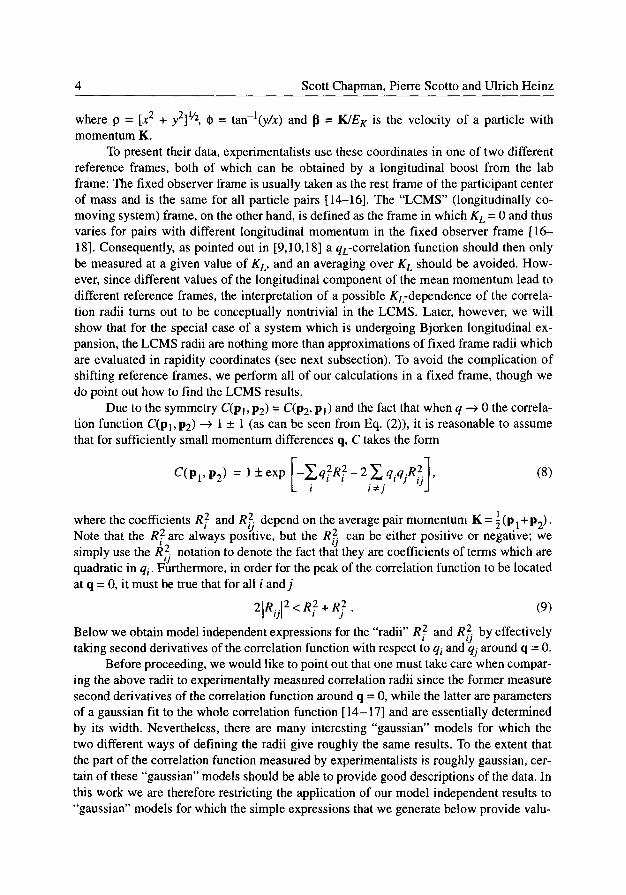
Fig. 3. The one particle spectrum obtained by numerically integrating (54) is plotted as a function of m t- m for midrapidity (Y = 0) pions and kaons. The solid curve is for pions with no transverse flow (v = 0), while the dashed curves are for pions (normalized to 1) and kaons (normalized to 2) with v = 0.5c. The other source parameters used are • o = 4 fm/c, R G = 3 fm, &l = 1.5 and T= 150MeV.


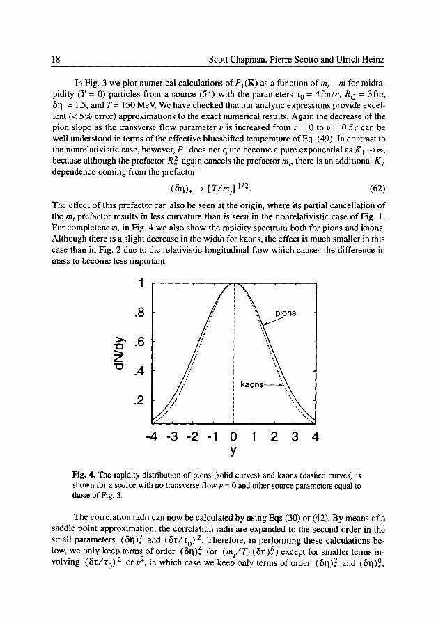
In Fig. 3 we plot numerical calculations of P I (K) a s a function of m t - m for midrapidity (Y = 0) particles from a source (54) with the parameters "c 0 = 4fm/c , R G = 3fm, ~Sr I = 1.5, and T = 150 MeV. We have checked that our analytic expressions provide excel- lent (< 5 % error) approximations to the exact numerical results. Again the decrease of the pion slope as the transverse flow parameter v i s increased from v = 0 to v = 0.5c can be well understood in terms of the effective blueshifted temperature of Eq. (49). In contrast to the nonrelativistic case, however, PI does not quite become a pure exponential as K• because although the prefactor R. 2 again cancels the prefactor tot, there is an additional K• dependence coming from the prefactor

(~1]) . --~ [ T / m t ] 1/2 (62)

The effect of this prefactor can also be seen at the origin, where its partial cancellation of the m t prefactor results in less curvature than is seen in the nonrelativistic case of Fig. 1. For completeness, in Fig. 4 we also show the rapidity spectrum both for pions and kaons. Although there is a slight decrease in the width for kaons, the effect is much smaller in this case than in Fig. 2 due to the relativistic longitudinal flow which causes the difference in mass to become less important.

Z

.8

.6

.4

.2

I p lons 7 ,, '.,

7 I ':

/ i \ ' o," i ~

, , t N

�9 " i I I I I I " .

-4 -3 -2 -1 0 1 2 3 4 Y

Fig. 4. The rapidity distribution of pions (solid curves) and kaons (dashed curves) is shown for a source with no transverse flow v = 0 and other source parameters equal to those of Fig. 3.

The correlation radii can now be calculated by using Eqs (30) or (42). By means of a saddle point approximation, the correlation radii are expanded to the second order in the small parameters (Srl), 2 and (~Z/Zo)2. Therefore, in performing these calculations below, we only keep terms of order (~Srl) 4 (or ( m t / T ) (~~rrl) 6) except for smaller terms involving (8"c/'c0) 2 or v 2, in which case we keep only terms of order (8rl) . 2 and (8~) 0,


respectively. Please note that for the source given in (54), no terms involving (Sx/xo) 4 or higher powers of this ratio occur in the results.

4.1. HBT Radii in Cartesian Coordinates

In cartesian coordinates, the correlation radii take the following form (ordered by powers of the small expansion parameters (8x/'%) 2 and (&q)2):

R 2 = R,2; s

R 2 = R, 2 + K2 K 2 _ _ "'-L R2~.2 ( 5 1 ] ) 2 m2 ( I~I;)2 + m2VL-O

+ m Ÿ 1 Y (Sx)2(Srl),2

• 2 2 + - - x [3 v - Y L mŸ 0 2I]L (--~q) 2 + (81])4;

m 2 m 2 m 2 7gvx0(Sq) , , RL2= ~_2KK,I7£ (8q)2 + ~_.2KK (Sq;)2(STi)2 +/SKt 2 4.

R Ÿ L 2 8 2 ~I_[~JL Y - -la• o ( q ) , - ] (8,t) 2 (Srl) 2 (81] ) 2

(8~) 2

(63)

Here v = 1 + (R, /RG)2- I 2 5 (mt/T)(81])*, and we have neglected the corrections which come from using (2) instead of (6). Although this model is not completely gaussian, within the scope of our approximation R 2 still roughly measures the transverse region of s homogeneity of the fluid, as can be seen by comparing (60) with (19). Although we will show that in practice all terms given in (63) are important, we will for didactical purposes first consider only the leading order in the small expansion parameters. Then the expressions (63) simplify and can be reformulated as follows:

1 1 1 mt v 2 -- -- .4.

R~ Ri =~ T R~'

R~ = ~~o (Sn) + r ~I) (64)

1 - 1 ( 1 mtl I


In agreement with [10] we find that, in each p¡ direction of the expanding fireball, two length scales should be distinguished. In addition to the geometric length scales R G

and L G = "~0813 in the transverse and longitudinal directions respectively, we have two "lengths of homogeneity" generated by the flow gradients. The transversal and longitudinal homogeneity lengths ate given by the following expressions:

T R 2 T 2

R 2 - m i v2 , L 2 = m---ir'CO. (65)

Please note that the occurrence of x o in both longitudinal lengths, L G and L H, has two different origins: whereas the geometrical longitudinal extension of the fireball at freeze-out is clearly always proportional to the mean freeze-out proper time %, its occurrence in the longitudinal homogeneity length is due to the specific choice of the velocity profile, since for a longitudinally boost invariant velocity profile the velocity gradient is just given by the inverse proper time. In fact, the true origin of the homogeneity lengths (65) is seen by writing them in the form

R2 - T 1 m t (3v&/ap) 2'

L2H - m t ( ~ ~ u ~ ) 2 ,

"r = "~0

(66)

where v• = vp, and in the second line u~ = (chrl, 0, 0, shrl) denotes the longitudinal part of the flow velocity profile (56) which satisfies a~tu ~ = ( 1 /~) . Eq. (66) makes the nature of the homogeneity lengths explicit in showing how they are generated by the flow gradients at freeze-out. For T---> 0, the lengths of homogeneity R H, L H vanish because in this limit only a single point in the source (namely the one where the fluid velocity agrees with the velocity of the pion pair) contributes to the correlation function at a given value of K. For T ~ ~, the homogeneity lengths also approach ~, because the thermal momentum distribution becomes flat and thus smears out the velocity gradients, thereby prohibiting the decorrelation of different fireball regions with large relative fluid velocities.

With these notations, the correlation radii can be written as follows:

1 1 1 - + _ _ ;

1 1 1

R 2 = /?2 + p 2 ; o ~ ~) ,67, c h 2 y ( -~1 + ; 1

R~ t.L~


As already pointed out in [10], the correlation radii are seen to be dominated by the shorter of the geometric and homogeneity lengths. This means in particular that if v ~ 0, then R 2

s

will be smaller than the geometrical radius R G. As the transverse mass increases, this reduction of R s and R• relatively to the pure geometric radius becomes more pronounced.

In the longitudinal direction, as a general consequence of the particle pair motion with velocity Y, the system appears Lorentz-contracted. Hence qL-correlation functions at finite values of Y measure longitudinal correlation radii, which are reduced by the corresponding Lorentz-contraction factor ch-lY, as shown by (67). Similar purely kinematic factors affect the out-longitudinal radius R•

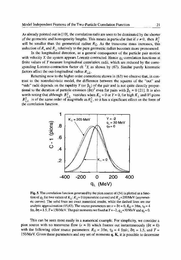
Returning now to the higher order corrections shown in (63) we observe that, in contrast to the nonrelativistic model, the difference between the squares of the "out" and "side" radii depends on the rapidity Y (or 13L) of the pair and is not quite directly proportional to the duration of particle emission (Sx) 2 even for pairs with I~L = 0 [21]. It is also worth noting that although RŸ vanishes when K• = 0 or Y= 0, for high K• and IYI pions R2 L i s of the same order of magnitude as RL2, so it has a significant effect on the form of the correlation function.

K_L = 200 MeV Y = -2 \ q• 30 MeV 0.8 ~~:o

~ . 6

' ,,;':'i': ''"i 0 .4

.2 'K~ = 0

-400 -200 0 200 4 0 0

qL (MeV)

Fig. 5. The correlation function generated by the pion source of (54) is plotted asa function ofqL for two values of K• K_L= 0 (symmetric curves) and K• (asymmet- tic curves). The solid lines are exact numerical results, while the dashed lines are our analytic approximation (15,63). The source parameters are v = 8"~ = 0, R G = 3fm, x 0 = 4 fm, ~ = 1.5, T= 150 MeV. The pair momenta we fixed at Y=-2, q• MeV and qs = O.

This can be seen most easily in a numerical example. For simplicity, we considera pion source with no transverse flow (v = 0) which freezes out instantaneously (~ix = 0) with the following other source parameters: R G = 3fm, "~0 = 4 fm/c, �91 = 1.5, and T = 150MeV. Given these parameters and any set of momenta q, K, it is possible to determine


the correlation function both by using the approximate radii of (63) and by performing an exact nume¡ calculation of the correlation using (2) and (54). In all of our plots of the correlation function, solid curves are used to denote numerical calculations, while dashed curves are used to denote our analytic approximation.

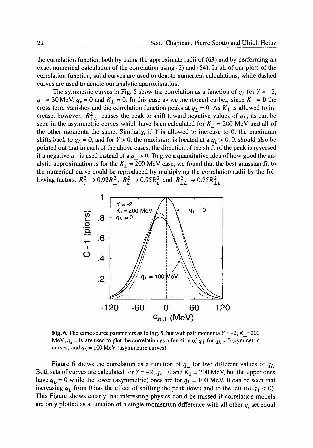
The symmetric curves in Fig. 5 show the correlation a s a function of qL for Y = - 2 , q_L = 30MeV, qs = 0 and K_L = 0. In this case as we mentioned earlier, since K• = 0 the cross term vanishes and the correlation function peaks at qL = 0. As K• is allowed to increase, however, R2 L causes the peak to shift toward negative values of qL, as can be seen in the asymmetric curves which have been calculated for K L = 200 MeV and all of the other momenta the same. Similarly, if Y is aliowed to increase to 0, the maximum shifts back to qL = 0, and for Y > 0, the maximum is located at a qL > 0. Ir should also be pointed out that in each of the above cases, the direction of the shift of the peak is reversed if a negative q• is used instead of a q_L > 0. To give a quantitative idea of how good the analytic approximation is for the K L = 200 MeV case, we found that the best gaussian fit to the numerical curve could be reproduced by multiplying the correlation radii by the fol- Iowing factors: R 2 --) 0 .92RŸ RL2 ---~ 0.95RL2 and RŸ --> 0.75R2 L.

(/'} t- o ~ Q. v

!

o

.8

.6

.4

.2

-120

u _--2 / , \ ~=2oo Mov/.i\' qs =0 """ '

/ i <'i ~ ' L ---= ~Me ~ v , , ; q L = 1 O0 MeV

-60 0 q0ut (MeV)

qL=O

< - - r

60 120

Fig. 6. The same source parameters as in Fig. 5, but with pair momenta Y= -2, K_L=200 MeV, qs = 0, are used to plot the correlation asa function of q_L for qL = 0 (symmetric curves) and qz. = 100 MeV (asymmetric curves).

Figure 6 shows the correlation a s a function of q_L for two different values of qL. Both sets of curves are calculated for Y= - 2 , qs = 0 and K_L = 200 MeV, but the upper ones have qL = 0 while the lower (asymmetric) ones are for qL = I00 MeV. It can be seen that increasing qL from 0 has the effect of shifting the peak down and to the left (to q_L < 0). This Figure shows clearly that interesting physics could be missed ir correlation models are only plotted a s a function of a single momentum difference with all other qi set equal


to zero. Again to get a quantitative idea of the validity of the analytic approximation, we found that the best gaussian fit to the numerical curve for qL = 100 MeV could be obtained using the factors R 2 ---~ 0 .85RŸ ,RŸ --~ 1.08R 2, and R2 L ---~ 0.75R~L.

As can be seen from Figs 5 and 6, the simple analytic expressions of (63) reproduce the exact correlation functions remarkably well considering the crudity of the approximation. By extensively exploring the parameter space of the model, we have found that the quantitative error estimates we have obtained in Figs 5 and 6 are somewhat typical of the maximum discrepancies for reasonable parameters. Namely, the analytic approximations of (63) for R 2, RL2 and R~_ L are able to reproduce the best gaussian fits to the numerical expressions to within < 20%, < 10%, < 33 %, respectively (e.g. for R2 L, (1 - 0.75)/0.75 ~ 33%). Although not shown, the analytic expressions for R 2 are much better, their dis- crepancy from numerical fits is typically ~< 5 %. We would also like to note that we have performed numerical calculations using Eq. (6) and find them to agree to within 3 % with numerical calculations using (2), so we are well justified in neglecting those corrections in Eqs (63).

r,I)

o

I

o

.8

.6

.4

.2

-150

Y = +2 i KJ. = 2 0 0 M e V ', qL = 1 5 0 M e V ~ q

-75 0 75 150

qout (MeV)

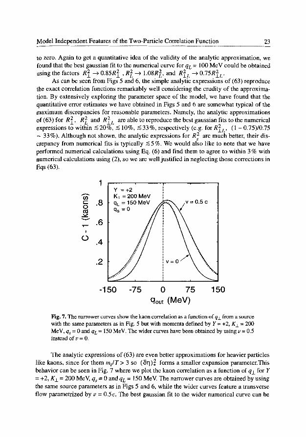
Fig. 7. The narrower curves show the kaon correlation as a function of q• from a source with the same parameters as in Fig. 5 but with momenta defined by Y = +2, K• = 200 MeV, qs = 0 and qL = 150 MeV. The wider curves have been obtained by using v = 0.5 instead of v = 0.

The analytic expressions of (63) are even better approximations for heavier particles like kaons, since for them mt/T > 3 so (Srl) 2 forms a smaller expansion parameter.This behavior can be seen in Fig. 7 where we plot the kaon correlation a s a function of q_L for Y = +2, K• = 200 MeV, qs = 0 and qL = 150 MeV. The narrower curves are obtained by using the same source parameters as in Figs 5 and 6, while the wider curves feature a transverse flow parametrized by v = 0.5c. The best gaussian fit to the wider numerical curve can be


obtained in this case by multiplying the radii of the wider analytical curves by the factors R 2 ---)0.94RŸ R 2 --)1.02RL2, and R 2 L --~ 0 . 9 R 2 L.

Perhaps the best way to study the correlation function is to make a 2-dimensional surface plot of C - 1 as function of both q• and qL" Figure 8 shows such a plot of the numerical calculation of C - 1 for Y = -2, K_L = 200 MeV and qs = 0. The effect of the cross term can be seen in the form of a ridge running from the peak at q• = qL = 0 down to the front left where qL > 0 and q_L < 0. Since cylindrical symmetry precludes the existence of "side-out" or "side-longitudinal" cross terms, the only effect of averaging over qs from 0 to some maximum value such as 30 or 50 MeV [14] would be to reduce the intercept o f the correlation function to some value less than 1. This averaging, however, should have very little impact on the qualitative ridge structure of the "out-long" correlation function. Consequently, this kind of ridge should be clearly identifiable experimentally and in fact may have already been seen in preliminary E802 correlation data [22].

1

C-1

.5

ooOo~ n , 4 0 0 ~ ' ' '

" -120 -60 0 60 120

qout (MeV) Fig. 8. The numerically calculated correlation function generated by the pion source of Fig. 5 is plotted asa function of qL and q• for Y = -2, K• = 200 MeV and qs = 0.

Before analyzing this model in rapidity coordinates, we would like to note that the LCMS radii o f this model can be obtained simply by setting 13 L = 0 and E K = m t in (63). Note that the factor of Y in R 2 L should not be set equal to zero, since it arises from the space-time rapidity distribution of the point-like sources in (54) which obviously breaks the boost invariance of the emission function in the longitudinal direction [23]. Transform- ing to the LCMS frame introduces a Ydependence which eventually translates into a non- vanishing cross term. We would like to emphasize that, to the first order in the small expansion parameters, our results reduce to the expressions for the LCMS correlation radii derived in [10]. However, in the light of a comparison of the results obtained within the framework of our analytical approximation with an exact numerical computation of the


correlation function, it turns out that the second order contributions to the correlation radii must be included. In particular, the out-longitudinal cross terms, whose effect can be clearly seen in Fig. 8, is completely missed at leading order. Nevertheless, for this model, the LCMS frame has the advantage that the expressions for the correlation radii are much simpler than for those in the fixed frame. On the other hand, this same simplicity can be achieved without the complication of reference frame shifting by expressing everything in terms of boost-invariant coordinates, as we will now show.

4.2. HBT Radii in Boost-lnvariant Coordinates

Using the model independent expressions of (42) along with the emission function of (54), we obtain the following correlation radii

R 2 = R 2,

+ • I R 2 = R2 [ + (~.q)2 (~~)2 + ~ ( ~ n ) 4 ~ ,

K• R2y - ( ~ ~ (~TI),2 E ({~TI)2,2 + (~g)23,

(68)

where in contrast to section 4.1, Yis now defined Y = ~ (Yl + Y2) �9 Note also that in contrast to the corresponding radii of (63) R• and ~ in the above approximation are both independent of rapidity. In addition, the cross term R• will be small compared to these radii, especially for higher mass particles like kaons which have (St I) 2 << 1 or for future ultra- relativistic collisions in which (81"1) >> 1.

The astute reader will note that aside from a difference in the definition of Y, the fixed frame correlation radii of the last subsection can be easily derived from those of (68) in the following way: First insert the radii of (68) into the expression (34) for the correlation function, then make the replacement y --+ qL/EK- ~LK• q• 2, rewrite the resulting expression in the form of Eq. (15), and finally read off the radii of Eq. (63). The reason for this can easily be seen by noting that

K• q . x -~ q_l_-~- ~ ch(rl - Y) - Ymtxsh ('q - Y) - q• - qsY

t (69)

~- q• m---7 "c ch(rl - Y) - -E-qL - ~Lq• "~sh (TI - Y) - q• - qsY,

l where in the top line Y = ~ (y t + Y2)' while in the bottom line Y= ~ In [(E K + KL)/(E•- KL) ] . Note that in particular the LCMS radii can be found simply by making the replacement y-~qffm t. Based on this equivalence, one can see that for systems undergoing Bjorken longitudinal expansion, LCMS correlation functions are nothing more than approximations of fixed frame correlation functions in rapidity coordinates. Since the latter formula-


tion is manifestly boost invariant and avoids the complications arising from the introduc- tion of the different LCMS-reference frames, it is much more desirable to use those coor-

1 dinates. For the remainder of this section, we use the definition Y = 5 (Yl + Y2) �9

.6 " I r " " - i

@ ** p

- i ro .4 ..:: j

.2 ~ o" Ik

- . 4 - . 2 0 .2 .4

Y = Yl - Y2

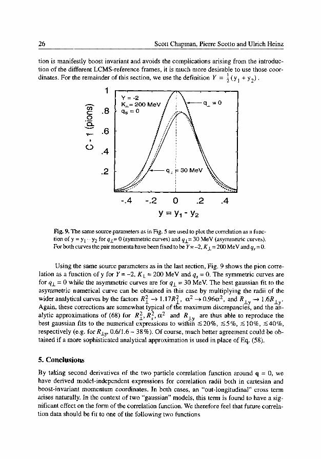
Fig. 9. The same source parameters as in Fig. 5 are used to plot the correlation as a function of y = Yl - Y2 for q_L= 0 (symmetric curves) and q_L = 30 MeV (asymmetric curves). For both curves the pair momenta have been fixed to be Y=-2, K.L = 200 MeV and qs = O.

Using the same source parameters as in the last section, Fig. 9 shows the pion correlation a s a function of y for Y = -2, K• = 200 MeV and qs = 0. The symmetric curves are for q./_ = 0 while the asymmetric curves are for q.L = 30 MeV. The best gaussian fit to the asymmetric numerical curve can be obtained in this case by multiplying the radii of the wider analytical curves by the factors R 2 --~ 1.17RŸ O~ 2 ~ 0.96~ 2, and R_Ly ~ 1.6R_Ly. Again, these corrections are somewhat typical of the maximum discrepancies, and the analytic approximations of (68) for R 2, R2s' ct2 and R_Ly are thus able to reproduce the best gaussian fits to the numerical expressions to within ~< 20%, < 5 %, < 10%, < 4 0 % , respectively (e.g. for R_l_y, 0.6/1.6 - 38%). Of course, much better agreement could be obtained if a more sophisticated analytical approximation is used in place of Eq. (58).

5. Conclusions

By taking second derivatives of the two particle correlation function around q = 0, we have derived model-independent expressions for correlation radii both in cartesian and boost-invariant momentum coordinates. In both cases, an "out-|ongitudinal" cross term aris•s naturally. In the context of two "gaussian" modr this term is found to have a significant effect on the form of the r function. We ther•fore fcel that future correlation data should be fit to one of the following two funr


/ h

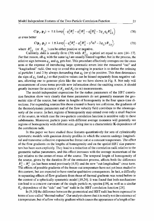
C(p 1 , P2) = 1 + ~,exp[- q 2 R 2 ~2o2 ~2o2 _ 2 q & q L R 2 L ) (70) k. s s - �91 l ' l - 91Li~L

or even better

- ( 2 2 2 2-y2ct2-2q_l_YR_l_y ), C(p r p2 ) = 1 + Lexp - q s R s - q.j_R_l - (71)

where R 2 L (or R, ) can be either positive or negative. &y Currently, data is usually fit to (70) with R 2 L a priori set equal to zero [14-17].

For that reason, all qi with the same Iqi I are usually binned together, but in the process, the relative sign between q_l_ and qL gets lost. This procedure effectively averages out the cross term at the expense of introducing large systematic errors into the measured "out" and "longitudinal" radii. One way to avoid this averaging in practice is to define the ordering of particles 1 and 2 by always demanding that qL (or y) be positive. This then determines the sign of q_l_ (and qs ) so that positive values can be binned separately from negative values, allowing one to generate plots like the one we have shown in Fig. 8. Not only will measurement of cross terms provide new information about the emitting source, it should greatly increase the accuracy of R_l - and R L (or o~) measurements.

The model-independent expressions for the radius parameters of the HBT correlation function show very clearly that these parameters do not generally measure the geometric size of the source, but rather its lengths of homogeneity in the four space-time directions. For expanding sources like those created in heavy ion collisions, the gradients of the thermodynamic parameters and of the flow velocity field contribute to the inhomogeneity of the source. In fact, regions of homogeneity may extend over only a small fraction of the source, in which case the two-particle correlation function is sensitive only to these subdomains. Moreover, particle pairs with different average momenta will generally see regions of homogeneity with different size, giving rise to a characteristic K-dependence of the correlation radii.

In this paper we have studied these features quantitatively for sets of cylindrically symmetric models with gaussian density profiles in which the sources undergo longitudinal and transverse collective expansion but freeze out at a constant temperature. The effect of the flow gradients on the lengths of homogeneity and on the spatial HBT size parameters has been seen explicitly. They lead to a reduction of the correlation radii retative to the geometric radius parameters, and this effect increases with the average momentum of the pair relative to the center-of-mass of the source. The temporal length of homogeneity of the source, given by the duration ~'c of the emission process, affects both the difference R2 - R2s (as has been noted previously [4,9]) and the new "out-longitudinal" cross term. The effects of possible gradients of the freeze-out temperature have not yet been studied in this context, but are expected to have similar qualitative consequences. In fact, a difficulty in separating effects of flow gradients from those of thermal gradients was noted before in the context of a spherically symmetric model [19,24]. It was found that both mechanisms can lead to a concave curvature of the single particle mt-spectra [19], as well a s a similar K_cdependence of the "side" and "out" radii in the HBT correlation function [24].

In [9,10] the difference between the geometrical and HBT radii has been expressed in terms of a so-called "thermal radius". Our analysis shows that it is really not the existence of a temperature, but of a flow velocity gradient which causes the appearance of a length of ho-


mogeneity in the HBT radii. The temperature only plays a role asa smearing factor, and the ratio T / m t s e t s the scale at which the inhomogeneity of the flow field becomes effective. Dif- ferent flow velocities in the transverse and longitudinal directions generally lead to different transverse and longitudinal homogeneity lengths, R H and L H. In [9,10] this was not obvious because the flow gradient was fixed to be 1/'~0 in all directions by the choice of the flow velocity profile.

AII of our calculations in this paper were done in a fixed reference frame, thus avoiding the complications with the LCMS frame discussed in section 2. However, we found that by parametrizing the correlation function in terms of rapidities rather than longitudinal momenta, one finds a longitudinal correlation radius and an out-longitudinai cross term which for sources with boost-invariant longitudinal expansion can be well approximated by the LCMS results. Since this parametrization avoids the LCMS problems of shifting frames, we suggest that the concept of the LCMS be abandoned in favor of using rapidity coordinates. We also showed that the existence of an out-longitudinal cross term is not affected by this choice of coordinates or frames, although its actual size is.

The analytic expressions for the HBT size parameters developed in this paper have been tested numerically and were found to be sufficiently accurate for being useful in ob- taining good qualitative insights on the effects which various features of the source have on the shape of the correlation function. We also studied explicitly the usually neglected corrections due to the off-sheil nature of the average 4-momentum entering in the correlation function and found them to be very small (< 3 %). To the extent that our two models for the source emission function are reasonable approximations to reality, these relations can be used to study the effects of longitudinal and transverse flow and of the time and duration of the freeze-out process on the HBT data. We have checked that the models produce single particle spectra with reasonable shapes which very likely can be used for good fits to the data (in particular once resonance decays are included). A more detailed analysis of the HBT data in the framework of these models thus appears as an attractive project.

Appendix

In this appendix, we prove that in the limit K l - --) 0, R 2 ---) R 2 and the cross term of either Eq. (30) or Eq. (42) vanishes (depending on the coordinate system used). The cru- cial ingredient of the proof is that the emission function is a Lorentz scalar whose K dependence only enters in the form of scalar products with cylind¡ symmetric local 4-vectors. For simplicity in the foliowing, we will assume that there is only one such local 4-vector, but generalization to the emission function of (10) can be done trivially.

We assume an emission function of the form

S(x, K) = 7S(t, p, z, m 2, ~/), (72)

where in a cartesian coordinate system

= K . u(x) = EKUo-K.l_UpCOS r - K L u z (73)

and u 0, up, and u z are independent of r Using rapidity coordinates as in (32) and (39) on the other hand, we can see that


~1 = m t u t c h ( Y - ~) - K_LUpCOS r (74)

where u t, ~ and up are independent of ~. In either case, as Iong as the ~ dependence of S is smooth, it follows that

lira I d 4 x c o s ~ f( t , p, z )S = O, K• O'

lim J'd4xcosr f(t, p, z)~-~ = 0, (75) K• 0

lim I d 4 x c o s r p, z)32~ = 0 K• 0"

for any r functionf. From the first of the above equations we can see that

lim �91 p, z)cosr = 0 (76) K•

in particular (x) = (pcosr = 0, and consequently the non-derivative terms of R 2 L and R_Ly vanish in the limit K.t" ---) 0. Furthermore, since

1 lim (p2cos2~)= lim (p2s in2r ~(p2), (77) K• 0 K.I.---) 0

i.e. (x 2) = (y2) = ~(p2), it can be seen that the non-derivative terms of R 2 equal those of Rs2 in that limit.

As for the momentum derivative terms, from Eq. (75) we have

d Sd4xupCOSr lim ~ P t ( K ) = - = 0 K • O U JX .l - "

(78)

in either set of coordinates. Similarly,

d d d d lim _ PI(K) = lim PI(K) = 0. (79)

K•162 0 d K L dK_ L K• 0 d Y dK_l"

Since

dKL d-~•177 ) [P, (K)I2(-~L)t ,---~~ ) (80)

we have proved that R~L of (30) vanishes for K j_ ~ 0. The proof for R_Ly follows simply by replacing d / d K L with d / d Y in the above equation.

The momentum derivative term for the "out" radius does not vanish in this limit, rather in the cartesian system ir takes the form

d 2 + lim d---~--& PI(K)= lim ~d4x(•176176 �91 u2 .o2a.~2~~ (81)

K• Kj_-"~O ~. K OV pCu~ V0~Iq ).


The derivative term for the "side" radius is a bit trickier since it involves a ratio of two quantities which vanish in the K• --~ 0 limit

�9 I d l imSd4x( u I .__20 up �91 S hm - ~ - ~ P I ( K ) = + K l ~ 0 ^ i a ~ ' i KilO ~E K ~ c o s r �91 (82)

Determination of the appropriate limit of the second term above is found by the rule of l'Hospital by dividing the derivative (with respect to h i ) of the numerator by the deriva- tire of the denominator. When this is done, the results for the "side" and "out" directions become identical. A similar argument can be used to show the same thing in the rapidity coordinate system.

Acknowledgements

We would like to thank T. Cs6rg‰ and T. Alber for clarifying and stimulating discussions. This work was supported in part by BMBF, DFG, and GSI.

References

1. D. Boal, C.K. Gelbke and B. Jennings, Rev. Mod. Phys. 62 (1990) 553. 2. G.E Bertsch, P. Danielewicz and M. Herrmann, Phys. Rev. C49 (1994) 442. 3. E. Shuryak, Phys. Lett. B44 (1973) 387; Soy. J. NucL Phys. 18 (1974) 667. 4. S. Pratt, T. Cs6rg£ and J. Zim• Phys. Rev. C42 (1990) 2646. 5. I.V. Andreev, M. Plª and R.M. Weiner, Int. J. Mod. Phys. A8 (1993) 4577. 6. S. Chapman and U. Heinz, Phys. Lett. B340 (1994) 250. 7. S. Chapman, P. Scotto and U. Heinz, submitted to Phys. Rev. Lett., in press. 8. Y. Sinyukov, in Hot Hadronic Matter: Theory and Experiment, eds, J. Letessier et al.,

Plenum, New York, 1995, in press. 9. T. Cs6rg£ B. L~rstad and J. Zim• Phys. Lett. B338 (1994) 134.

10. T. Cs6rg£ Lund preprint LUNFD6 (NFFL -7081) (1994), Phys. Lett. B, in press; T. Cs6rg£ B. Lcrstad, Lund preprint LUNFD6 (NFFL -7082) (1994).

11. M. Gyulassy, S.K. Kauffmann and L.W. Wilson, Phys. Rey. C20 (1979) 2267. 12. B.R. Schlei et al., Phys. Len. B293 (1992) 275; J. Bolz et al., Phys. Lett. B300 (1993)

404. 13. A.N. Makhlin and Y.M. Sinyukov, Soy. J. Nucl. Phys. 46 (1987) 345. 14. NA35 Colh, T. Alber et al., Phys. Rev. Lett. 74 (1995) 1303. 15. NA35 Colh, G. Roland et al., Nucl. Phys. A566 (1994) 527c; NA35 Coll., D. Ferenc et

al., Frankfurt preprint IKF-HENPG/2-94 (1994); NA44 Coll., M. Sarabura et al., Nucl. Phys. A544 (1992) 125c; E802 Coll, T. Abbott et al., Phys. Rev. Lett. 69 (1992) 1030.

16. NA35 Col[, P. Seyboth et al., Nucl. Phys. A544 (1992) 293c; NA35 Coll., D. Ferenc et al., Nucl. Phys. A544 (1992) 531c.

17. NA44 Coll., H. Beker et al., CERN-PPE/94-119, submitted to Phys. Rev. Lett. 18. T. CsiSrg6 and S. Pratt, Lund Preprint LU TP 91-10, in Proc. of the Workshop on

Relativistic Heavy Ion Physics, preprint KFKI-1991 - 28/A, p. 75.


19. K.S. Lee, E. Schnedermann and U. Heinz, Z. Phys. C48 (1990) 525. 20. A. Makhlin and Y. Sinyukov, Z. Phys. C39 (1988) 69. 21. This was not seen in [10] where only the first order corrections were calculated in the

LCMS frame, I]L=0. 22. M. Gyulassy, Lecture given at the Budapest Workshop on High Energy Heavy Ion

Physics, August 25-28, 1994. 23. From Eq. (30) one sees that in the LCMS frame (denoted by primed variables as in

(52)) the cross term is given by:

~tt (('c2chrl'sh~ ') - (zchrl ')

up to small logarithmic corrections. This clearly vanishes as soon as the source S(x,K) becomes reflection symmet¡ under r 1' -~ -ti ' . Please note that for a longitudinally boost invariant velocity profile, this symmetry is broken only by the space-time rapidity distfibution of point-like sources.

24. U. Mayer, E. Schnedermann and U. Heinz, Phys. Lett. B294 (1992) 69.

Documents

Model independent features of the two-particle correlation function