Model-independent particle accelerator tuning

Alexander Scheinker,* Xiaoying Pang,† and Larry Rybarcyk‡

Los Alamos National Laboratory, Los Alamos, New Mexico 87545, USA(Received 25 July 2013; published 21 October 2013)

We present a new model-independent dynamic feedback technique, rotation rate tuning, for automati-

cally and simultaneously tuning coupled components of uncertain, complex systems. The main advan-

tages of the method are: (1) it has the ability to handle unknown, time-varying systems, (2) it gives known

bounds on parameter update rates, (3) we give an analytic proof of its convergence and its stability, and

(4) it has a simple digital implementation through a control system such as the experimental physics and

industrial control system (EPICS). Because this technique is model independent it may be useful as a real-

time, in-hardware, feedback-based optimization scheme for uncertain and time-varying systems. In

particular, it is robust enough to handle uncertainty due to coupling, thermal cycling, misalignments,

and manufacturing imperfections. As a result, it may be used as a fine-tuning supplement for existing

accelerator tuning/control schemes. We present multiparticle simulation results demonstrating the

scheme’s ability to simultaneously adaptively adjust the set points of 22 quadrupole magnets and two

rf buncher cavities in the Los Alamos Neutron Science Center (LANSCE) Linear Accelerator’s transport

region, while the beam properties and rf phase shift are continuously varying. The tuning is based only on

beam current readings, without knowledge of particle dynamics. We also present an outline of how to

implement this general scheme in software for optimization, and in hardware for feedback-based control/

tuning, for a wide range of systems.

DOI: 10.1103/PhysRevSTAB.16.102803 PACS numbers: 41.85.Lc, 02.30.Yy, 29.20.�c, 02.60.�x

I. INTRODUCTION

A. Motivation

It is rarely possible to build exact, deterministic input tooutput models for complex physical systems such asparticle accelerators. It is especially difficult when thebehavior of the system is influenced by many coupledparameters. Since accelerators have many coupled parame-ters, they are prime candidates for genetic algorithm (GA)and multiobjective genetic algorithm (MOGA) based mul-tidimensional, nonlinear optimization schemes. In fact,MOGAs and GAs have been used to successfully optimizemany aspects of particle accelerators, such as magnet andradio frequency (rf) cavity design [1], photoinjector design[2], damping ring design [3], storage ring dynamics [4],global optimization of a lattice [5], neutrino factory design[6], simultaneous optimization of beam emittance anddynamic aperture [7], and free electron laser linac drivers[8]. A thorough review of GA for accelerator physicsapplications is given in [9].

After an accelerator design has been finalized and theaccelerator has been constructed, one often encounters

time-varying and nonlinear coupling effects between theimperfectly manufactured and misaligned/unknown orien-tation components of the accelerator. In theory, acceleratordesign takes a certain level of uncertainty into account. Inpractice however, most accelerators require postmanufac-ture and postinstallation tuning. This is especially the casefor facilities with limited real-time diagnostics and noisemeasurement. In this case components may have to beretuned after each shutdown or change in operating con-ditions. Effects such as unknown hysteresis curves andtime-varying component thermal cycling also add to sys-tem uncertainty. A particular problem faced by manyaccelerator systems is the arbitrary phase shift of the rfsystems, a time-varying uncertainty, requiring time con-suming tuning such as phase scans. The method presentedhere is demonstrated to automatically adapt for time-varying properties, such as phase shift. A combination ofthe global optimization abilities of GAs, with a local,model-independent feedback technique such as the onepresented here, has the potential to improve acceleratordesign and performance.

B. Results of the paper

In this work, we present a simple, model-independenttechnique, which can aid in parameter tuning because itdoes not, by design, assume any particular system modelfor optimizing/tuning and therefore may be implementedin hardware to automatically fine-tune multiple parametersand help mitigate unmodeled disturbances and componentimperfections.

*ascheink@lanl.gov†xpang@lanl.gov‡lrybarcyk@lanl.gov

Published by the American Physical Society under the terms ofthe Creative Commons Attribution 3.0 License. Further distri-bution of this work must maintain attribution to the author(s) andthe published article’s title, journal citation, and DOI.

PHYSICAL REVIEW SPECIAL TOPICS - ACCELERATORS AND BEAMS 16, 102803 (2013)

1098-4402=13=16(10)=102803(10) 102803-1 Published by the American Physical Society

For implementation, the user first defines a measurablecost function, C, to be minimized, whose analytic formmay be unknown, such as the total particle loss along thelength of a particle accelerator. The components pi of thevector p ¼ ðp1; . . . ; pmÞ are parameters by which the costmay be influenced, such as the power source current set-tings feeding the quadrupole magnets in the acceleratorlattice. The rotation rate (RR) tuning law is

piðnþ 1Þ ¼ piðnÞ þ�ffiffiffiffiffiffiffiffiffi�!i

pcosf!in�þ kC½pðnÞ�g: (1)

Initial settings pð1Þ are chosen as usual, based on a physicsmodel and a MOGA or other numerical optimization tech-nique. The initial cost, C½pð1Þ�, is calculated after the firstrun and new parameter values pð2Þ are set according to (1).The waiting time between implementation n and nþ 1 ischosen depending on component response/settling rates,data acquisition rates, and the rate of time variation ofsystem components due to disturbance. Intuitively, � isthe magnitude of a high frequency (!i) dither being intro-duced into the system’s dynamics, k is the gain of thecontroller/tuning algorithm, and � is a time interval fordigital implementation. The choices for the values of !i,�, k, and � are discussed in detail in Sec. III.

We demonstrate, through a multiparticle simulation ofthe Los Alamos Neutron Science Center (LANSCE) lowenergy beam transport region, RR’s ability to handle un-certainty by tuning up a 22 quadrupole lattice, and thephases of two rf buncher cavities, by minimizing a costwhich is based on beam current loss along the transportregion and the first two tanks of the drift tube linac, for atime-varying beam and time-varying rf phase drifts.

The RR approachmay also be used as a simple numericaloptimizer, in which adding new parameters pmþ1; pmþ2; . . .to (1) does not add significantly to computation time.Multiobjective optimization is implemented by replacinga single cost, C, with a combination C ¼ C1 þ � � � þ Cn,for any number of costs, such as C1 being total beam loss,C2 being total transverse beam size, etc. Also, differentparameters may be updated based on different rates andcosts (as in Sec. IVA), where components having differentsensitivities may require different values of ki and �i. Forexample, we may implement

piðnþ1Þ¼piðnÞþ�ffiffiffiffiffiffiffiffiffiffiffi�i!i

pcosf!i�nþkiCi½pðnÞ�g; (2)

for notational simplicity, we stick to single values ofk, �, and C throughout the analysis performed, which isapplicable in the same manner to the above, more generalscheme (2). Imposing restrictions on the parameters isstraightforward and implemented as described in Sec. III.

As shown in the analysis in Sec. II B, the scheme (1) ischosen so that, with proper choices of!, k, �, and�, (1) isthe finite difference approximation of

_p i ¼ ffiffiffiffiffiffiffiffiffi�!i

pcosf!itþ kC½pðtÞ; t�g; (3)

which on average follows the same trajectory as the system

_�p i ¼ � k�

2

@C½ �pðtÞ; t�@ �pi

; (4)

where the convention used here and throughout the remain-

der of the paper is _p ¼ @p@t .

RR is related to dithering-based optimization/stabilizationschemes, known in control theory as extremum seeking (ES),which have been used for optimizing unknown outputsof known, stable systems, by tuning known controllers.Originally introduced in 1922 [10], an overview of its devel-opment is available in [11]. Recently, ES has been extended toperform stabilization and optimization of unknown, possibleunstable systems [12]. RR is a further improvement andmodification of those results [13].

C. Optimization schemes

There are many existing model dependent numericalmethods for multidimensional/multiparameter optimiza-tion, such as GA, MOGA, Newton-Raphson and gradientdescent based on the analytic form of rC. Many optimi-zation methods are actually built into existing acceleratordesign codes [14].The main strength of RR is its model-independent nature

and ability to deal with multiple parameters simulta-neously, even for time-varying systems, such as thermalcycling, or unexpected component damage. Some verysimple, but computationally intensive and inefficient,model-independent methods are grid and random pointsearches, especially for systems with many parameters.Gradient descent, based on a numerical approximation ofan unknown rC is another model-independent approach,but especially in the case of a multiparameter, noisy cal-culation of C, may face difficulties, whereas RR is bothrobust to noise in C and does not need to try and estimaterC. Only samples CðnÞ are required.Simplex fitting, in the sense that it samples many different

directions inmultidimensional parameter space, has themostin common with RR. A major benefit of RR is that itscomplexity does not growwith parameter number, regardlessof the number of parameters being tuned. The scheme basi-cally depends on three choices, the values of k, !, and �.Regarding noisy data, the RR scheme is, on average, notinfluenced by noise, unless it happens to both match an RRparameter’s perturbation frequency and be large in magni-tude relative to that perturbation.Also, noise is easily handledby standard methods, such as averaging and filtering.

D. Limitations

Although RR is model independent and able to tunemany parameters simultaneously, unlike GA, it is a localtechnique, similar to gradient descent, and may becometrapped in local minimums. Therefore, we plan on explor-ing (in future work) a combination of GA and RR, in whicha GA is first used for global optimization followed by RRfor local, in-hardware tuning, to make up for modelingerrors and time variation.

SCHEINKER, PANG, AND RYBARCYK Phys. Rev. ST Accel. Beams 16, 102803 (2013)

102803-2

E. Organization

In Sec. II we give an explanation for the choice of theupdate scheme (1). In Sec. III we explain how to choose allRR parameters and describe digital implementation forgeneral systems. In Sec. IV, we demonstrate the scheme’sability to handle uncertainty by tuning a 22 quadrupolelattice as well as two rf buncher cavities, in a simulation ofthe LANSCE accelerator transport region and first twotanks of the drift tube linac, for a varying input beam anddrifting phase shifts. Finally, in Sec. V we provide back-ground regarding RR analysis.

II. TUNING METHOD

A. Physical motivation

It is well known that by adding a fast, small oscillationinto a system’s dynamics, unexpected stability propertiesmay be achieved. The classic example is of the invertedpendulum, whose vertical equilibrium point may be stabi-lized by rapidly vertically oscillating the pendulum’s pivotpoint. The dynamics of this process were first analyticallydescribed in the 1950s by Kapitza [15]. The RR schemehas some similarities to this approach, in that we introducehigh frequency oscillations into a system in order to forcecertain points of the state space to become stable equilib-rium points towards which the system’s trajectory con-verges. By abstracting this to a general state space andchoosing such a point to be the minimum of a cost func-tion, we are able to tune a wide range of systems towardsvarious performance goals.

We start with a simple example, we do not introduce anydestabilizing terms in (5) and (6), which are discussed inremark 1. To give a simple 2D overview of this method, weconsider finding the minimum of a measurable functionCðx; yÞ, for which we cannot simply implement a gradientdescent for the trajectory of ½xðtÞ; yðtÞ� because we areunaware of its analytic form. We propose the followingadaptive scheme:

@x

@t¼ ffiffiffiffiffiffiffiffi

�!p

cos½!tþ kCðx; yÞ� (5)

@y

@t¼ ffiffiffiffiffiffiffiffi

�!p

sin½!tþ kCðx; yÞ�: (6)

Note that although Cðx; yÞ enters the argument of theadaptive scheme, we do not rely on any knowledge of theanalytic form of Cðx; yÞ, we simply assume that its value isavailable for measurement at different locations ðx; yÞ.

The velocity vector,

v ¼�@x

@t;@y

@t

�¼ ffiffiffiffiffiffiffiffi

�!p fcos½�ðtÞ�; sin½�ðtÞ�g; (7)

where �ðtÞ ¼ !tþ kC½xðtÞ; yðtÞ�, has constant magnitude,k v k¼ ffiffiffiffiffiffiffiffi

�!p

, and therefore the trajectory ½xðtÞ; yðtÞ�moves at a constant speed. However, the rate at whichthe direction of the trajectories’ heading changes is afunction of !, k, and C½xðtÞ; yðtÞ� expressed as

@�

@t¼ !þ k

�@C

@x

@x

@tþ @C

@y

@y

@t

�: (8)

Therefore, when the trajectory is heading in the correctdirection, towards a decreasing value of C½xðtÞ; yðtÞ�, theterm k @C

@t is negative so the overall turning rate @�@t (8) is

decreased. On the other hand, when the trajectory is head-ing in the wrong direction, towards an increasing value ofC½xðtÞ; yðtÞ�, the term k @C

@t is positive, and the turning rate is

increased. On average, the system ends up approaching theminimizing location of C½xðtÞ; yðtÞ� because it spends moretime moving towards it than away.The ability of this direction-dependent turning rate

scheme is apparent in the simulation of system (5) and(6), in Fig. 1. The system, starting at initial locationxð0Þ ¼ 1, yð0Þ ¼ �1, is simulated for five seconds withupdate parameters ! ¼ 50, k ¼ 5, � ¼ 0:5, and Cðx; yÞ ¼x2 þ y2. We compare the actual system’s (5) and (6)dynamics with those of a system performing gradientdescent:

@ �x

@t� � k�

2

@Cð �x; �yÞ@ �x

¼ �k� �x; (9)

@ �y

@t� � k�

2

@Cð �x; �yÞ@ �y

¼ �k� �y; (10)

whose behavior our system mimics on average, with thedifference

maxt2½0;T�

k½xðtÞ; yðtÞ� � ½ �xðtÞ; �yðtÞ�k (11)

0.0 0.2 0.4 0.6 0.8 1.0

1.0

0.8

0.6

0.4

0.2

0.0

x

y

x,y Black Solid x , y Blue Dashed

0.0 0.1 0.2 0.3 0.4 0.5

20406080

100

t

tk

C x, yt

FIG. 1. The subfigure in the bottom left shows the rotation

rate, @�@t ¼ !þ @Cðx;yÞ

@t , for the part of the trajectory that is bold

red, which takes place during the first 0.5 seconds of simulation.The rotation of the parameters’ velocity vector vðtÞ slows downwhen heading towards the minimum of Cðx; yÞ ¼ x2 þ y2, atwhich time k @C

@t < 0, and speeds up when heading away from the

minimum, when k @C@t > 0. The system ends up spending more

time heading towards and approaches the minimum of Cðx; yÞ.

MODEL-INDEPENDENT PARTICLE ACCELERATOR TUNING Phys. Rev. ST Accel. Beams 16, 102803 (2013)

102803-3

made arbitrarily small for any value of T, by choosingarbitrarily large values of !. The derivation of thisrelationship and of the rate of the gradient descent aregiven in Sec. V.

Towards the end of the simulation, when the system’strajectory is near the origin, Cðx; yÞ � 0, and the dynamicsof (5) and (6) are approximately

@x

@t� ffiffiffiffiffiffiffiffi

�!p

cosð!tÞ ) xðtÞ �ffiffiffiffi�

!

rsinð!tÞ; (12)

@y

@t� ffiffiffiffiffiffiffiffi

�!p

sinð!tÞ ) yðtÞ � �ffiffiffiffi�

!

rcosð!tÞ; (13)

a circle of radiusffiffiffi�!

p, which is made arbitrarily small by

choosing small values of � or large values of!. A detailedoverview of how to choose the values k, �, and ! is givenin Sec. III. Convergence towards a maximum, rather than aminimum, is achieved by replacing k with �k.

B. General RR scheme

For general tuning, we consider the problem of locatingan extremum point of the function Cðp; tÞ: Rn � Rþ ! R,for p ¼ ðp1; . . . ; pnÞ 2 Rn, which we can measure thevalue of, but whose analytic form is unknown. For nota-tional convenience, in what follows we sometimes writeCðpÞ or just C instead of C½pðtÞ; t�.

The explanation presented in the previous section usedsinð�Þ and cosð�Þ functions for the x and y dynamics to givecircular trajectories. The actual requirement for conver-gence is for an independence, in the frequency domain,of the functions used to perturb different parameters, suchas sines or cosines of distinct frequencies. In what follows,replacing cosð�Þ with sinð�Þ throughout, or mixing sinð�Þand cosð�Þ terms makes no difference.

Theorem 1.—Consider the setup shown in Fig. 2 (formaximum seeking we replace k with �k):

_p i ¼ ffiffiffiffiffiffiffiffiffi�!i

pcos½!itþ kCðp; tÞ�; (14)

where !i ¼ !0ri such that ri � rj 8 i � j. The trajec-

tory of system (14) approaches the minimum of Cðp; tÞ,with its trajectory arbitrarily close to that of

_�p ¼ � k�

2rC; �pð0Þ ¼ pð0Þ (15)

with the distance between the two decreasing as a functionof increasing !0. Namely, for any given T 2 ½0;1Þ, anycompact set of allowable parameters p 2 K � Rm, andany desired accuracy �, there exists !?

0 such that for all

!0 >!?0 , the distance between the trajectory pðtÞ of (14)

and �pðtÞ of (15) satisfies the boundmax

p; �p2K;t2½0;T�kpðtÞ � �pðtÞk< �: (16)

Proof 1.—By expanding

cosð!itþkCÞ¼ cosð!itÞcosðkCÞ�sinð!itÞsinðkCÞ; (17)

we rewrite the pi (1 � i � n) dynamics as

_pi ¼ ffiffiffiffiffiffi!i

pcosð!itÞ

ffiffiffiffi�

pcosðkCÞ

� ffiffiffiffiffiffi!i

psinð!itÞ

ffiffiffiffi�

psinðkCÞ; (18)

and apply corollary 1 with respect to !0 and � ¼ 0:5. Thetrajectory of system (14) uniformly converges to the tra-jectory of

_�pi ¼ � k�

2

@Cð �p; tÞ@ �pi

fcos2½kCð �p; tÞ� þ sin2½kCð �p; tÞ�g

¼ � k�

2

@Cð �p; tÞ@ �pi

; (19)

where we have used the fact that mismatched terms of theform cosð!itÞ sinð!jtÞ, 8 i, j, and terms of the form

cosð!itÞ cosð!jtÞ, and sinð!itÞ sinð!jtÞ, 8 i � j weakly,

uniformly converge to zero. Combining all the pi compo-nents we get

_�p ¼ � k�

2rC: (20)

Remark 1.—The stability of this scheme is verified bythe fact that an addition of an unmodeled, possibly desta-bilizing perturbation of the form fðp; tÞ to the dynamics of_p results in the averaged system:

_�p ¼ fð �p; tÞ � k�

2rC; (21)

which may be made to approach the minimum of C, bychoosing k� large enough relative to the values ofkðrCÞTk and kfð �p; tÞk. Detailed stability analysis is avail-able in [12].Remark 2.—Although it is glossed over in the averaging

analysis presented above, if one looks into the details of theproof of theorem 2, in the case of a time-varying max/minlocation p?ðtÞ of Cðp; tÞ, there will be terms of the form

1ffiffiffiffi!

p��������@Cðp; tÞ

@t

��������; (22)

which are made to approach zero by increasing !.Furthermore, in the analysis of the convergence of the errorpeðtÞ ¼ pðtÞ � p?ðtÞ, there will be terms of the form

C(p1,...,p

n,t)

ui

pi(t)

cos(•)i

i t

C

k

1s

FIG. 2. Tuning of the ith component pi of p ¼ ðp1; . . . ; pnÞ 2Rn. The symbol 1s denotes the Laplace transform of an integrator,

so that in the above diagram piðtÞ ¼ pið0Þ þRt0 uið�Þd�.

SCHEINKER, PANG, AND RYBARCYK Phys. Rev. ST Accel. Beams 16, 102803 (2013)

102803-4

1

k�

��������@Cðp; tÞ

@t

��������: (23)

Together, (22) and (23) imply the intuitively obvious factthat for systems whose time variation is fast, in which theminimum towards which we are descending is quicklyvarying, both the value of ! and of the product k� mustbe larger than for the time-invariant case.

Remark 3.—In the case of different parameters havingvastly different response characteristics and sensitivities(such as when tuning both rf and magnet settings in thesame scheme), the choices of k and � may be specifieddifferently for each component pi, as ki and �i, withoutchange to the above analysis.

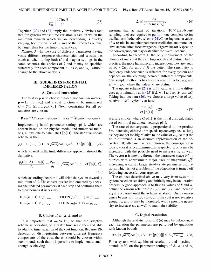
III. GUIDELINES FOR DIGITALIMPLEMENTATION

A. Cost and constraints

The first step is to choose tunable machine parameters,p ¼ ðp1; . . . ; pmÞ and a cost function to be minimized,C ¼ C½p1ðtÞ; . . . ; pmðtÞ; t�. Next, constraints for all pa-rameters are chosen:

p max¼ðp1;max; . . . ;pm;maxÞ; pmin¼ðp1;min; . . . ;pm;minÞ:Implementing initial parameter settings pð1Þ, which arechosen based on the physics model and numerical meth-ods, allows one to calculate C½pð1Þ�. The iterative updatescheme is then

piðnþ1Þ¼piðnÞþ�ffiffiffiffiffiffiffiffiffi�!i

pcosf!in�þkC½pðnÞ�g; (24)

which is based on the finite difference approximation of thederivative:

piðtþ �Þ � piðtÞ�

� @pi

@t¼ ffiffiffiffiffiffiffiffiffi

�!i

pcosf!itþ kC½pðtÞ; t�g;

(25)

which, according theorem 1 will drive the system towards aminimum of C. The constraints are implemented by check-ing the updated parameters at each step and confining themto their bounds if necessary:

IF piðnþ 1Þ> pi;max; THEN piðnþ 1Þ ¼ pi;max;

IF piðnþ 1Þ< pi;min; THEN piðnþ 1Þ ¼ pi;min:

B. Choice of !, �, k, and �

It is important that !i � kC, so that the adaptivescheme is operating on a faster time scale then and ableto adapt to time variation of the cost function. Because RRdepends on distinguishing between different frequencycomponents of the cost, the !i should be chosen withinsuch bounds such that it is possible to implement a smallenough � obeying

� � 2�

20�maxf!ig ; (26)

ensuring that at least 20 iterations (10� the Nyquistsampling rate) are required to perform one complete cosineoscillationintheiterativescheme(24).Choosingsmallervaluesof � results in smoother parameter oscillation and more iter-ativestepsrequiredforconvergence,largervaluesof�speedupthe convergence, but may destabilize the overall scheme.According to theorem 1, the only requirement on the

choices of!i is that they are big enough and distinct, but inpractice, the more harmonically independent they are (suchas !i � 2!j for all i � j) the better. The sensitivity to

frequency independence is different for every system anddepends on the coupling between different components.One simple method is to choose a scaling factor, !0, and!i ¼ !0ri, where the values ri are distinct.The update scheme (24) is only valid as a finite differ-

ence approximation as in (25) if� 1 and!i �ffiffiffiffi�

p; kC.

Taking into account (26), we choose a large value of !0,relative to kC, typically at least

minf!igkC½pð1Þ� > 20; (27)

is a safe choice, where C½pð1Þ� is the initial cost calculatedbased on initial parameter settings pð1Þ.The rate of convergence is proportional to the product

k�, increasing either k or� speeds up convergence, as longas they are not too big relative to the value of!0, so that thefinite difference is an accurate approximation of the de-rivative. If, after !0 has been chosen, the convergence istoo slow, or if a local minimum is suspected, k or �may beincreased, with the possible need to increase !0 as well.The vector p is moving through the parameter space Rm in

ellipses with approximate major axes of magnitudeffiffiffi�!

p,

increasing � causes larger steady state parameter oscilla-tions, which is not a problem if the adaptation is turned offfollowing successful convergence.The choices described above may vary from system to

system based on sensitivity and initially may be an iterativeprocess. A good approach is to first fix values of k and �,define the various relationships (26) and (27), and increase!0 if necessary until the scheme is stable. Once conver-gence begins, if it is too slow, or if the cost is not sensitiveenough, k and � may be increased, with a possible neces-sity to increase !0 as well to maintain stability.

C. Digital resolution

Although the analytic form of CðnÞ may be unknown, ateach iteration the parameters are perturbed by quantitieswith known bounds:

0�j� ffiffiffiffiffiffiffiffiffi�!i

pcosf!in�þkC½pðnÞ�gj��

ffiffiffiffiffiffiffiffiffiffiffiffiffiffi�!max

p: (28)

For a system with nb bits of resolution, and maximumbounds Mi on the parameter settings, if �, �, and !i

MODEL-INDEPENDENT PARTICLE ACCELERATOR TUNING Phys. Rev. ST Accel. Beams 16, 102803 (2013)

102803-5

are chosen such that �ffiffiffiffiffiffiffiffiffi�!i

p � N � Mi

2nb , then, as cosð Þvaries between 0 and 1, it is possible for the parameter

value to take N discrete steps of minimum resolution Mi

2nb .

D. Normalization of parameters

Different parameters pi may require individual values ofki and �i, in which case normalizing the parameters towithin ½�1; 1� bounds may be useful. For example, at eachstep n, one may compute the cost CðnÞ based on parametersettings pðnÞ, then translate into the scaled parameterspsðnÞ:

ps;iðnÞ ¼2½piðnÞ � Cp;i�

Dp;i

; (29)

where Cp;i ¼ pi;maxþpi;min

2 and Dp;i ¼ pi;max � pi;min, bound-

ing each parameter within ½�1; 1�. We then perform theRR update,

ps;iðnþ 1Þ ¼ ps;iðnÞ þ �ffiffiffiffiffiffiffiffiffiffiffi�i!i

pcosf!in�þ kiC½pðnÞ�g;

(30)

force the scaled parameters to satisfy the constraints �1and 1, and transform back into unscaled parameter valuesin order to calculate the cost for the next iteration:

piðnþ 1Þ ¼ ps;iðnþ 1ÞDp;i

2þ Cp;i: (31)

IV. TUNING 22 QUADRUPOLE MAGNETSAND 2 BUNCHER CAVITIES

In this section we present simulation results of using theRR scheme to tune up the 22 quadrupole magnets and twobuncher cavities in the Los Alamos linear accelerator Hþtransport region, a simplified schematic of which is shownin Fig. 3. The simulations were done using a graphicsprocessing unit–accelerated online beam dynamics

simulator [16,17], which is being developed to predictbeam properties along the linac using real-time machineparameters. It can serve as a virtual beam experimentenvironment and contribute to the cost being minimizedby the RR optimizer, by providing pseudo-real-time esti-mates of beam sizes and current information in parts of themachine where diagnostics are not available. Currentlybeing demonstrated on the LANSCE low energy beamtransport (LEBT) and drift tube linac (DTL), simulatinga bunch of 32K macroparticles through the LEBT or DTLtakes fractions of a second, which is 40 times faster thanthe simple CPU version of the code.

A. Magnet tuning for beam transport

In a first, simple demonstration of the technique, weperform a simulation of only the LEBT, with all initialmagnet current set points set to 0A, and allowed to tune upbased purely on the RR scheme as described above, inwhich the four costs (j ¼ 1; 2; 3; 4) being minimized,

Cj ¼ ðIj � 0:013Þ2; (32)

were the square of the difference between initial beamcurrent 0:013A and total current making it through variousparts of the transport region, at which diagnostics areavailable. With reference to Fig. 3, the current is sampledat four locations, I1, following Q6, I2 following Q10, I3followingQ18, and I4 at the end of the transport region. Themagnets (i ¼ 1; . . . ; 22) were then updated according to

Qiðnþ 1Þ ¼ QiðnÞ þ ffiffiffiffiffiffiffiffiffi�!i

p�cos½!i�nþ kSiðnÞ�; (33)

where Si ¼ C4 þ C3 þ C2 þ C1 for Q1–Q6, Si ¼C4 þ C3 þ C2 for Q7–Q10, Si ¼ C4 þ C3 for Q11–Q18,and Si ¼ C4 for Q19–Q22, so that magnets only saw costswhich they were able to influence. For the tuning parame-ters, we chose k ¼ 250000, so that the amplified costs kSjin (33) took values between 0 and 300. The!i were chosen

Q1

Q2

Q3

Q4

Q5

Q6

Q7

Q8

Q9

Q10 Q

11Q

12Q

13Q

14 Q15

Q16

Q17

Q18

Qi-Quadrupole Magnet

Injector

Drift Tube Linac

Bend Magnet

Other Components (diagnostics/scrapers/jaws...)

Beam

Q19

Q20

Q21

Q22

Buncher

Pre BuncherMain Buncher

FIG. 3. Simplified schematic of the LANSCE Hþ injector and transport region.

SCHEINKER, PANG, AND RYBARCYK Phys. Rev. ST Accel. Beams 16, 102803 (2013)

102803-6

as !0ri, with !0 ¼ 1000 and ri uniformly distributedbetween 2.5 and 3.7, � ¼ 2�

20!22, and � ¼ 15. With these

values, !min

kCmax> 20.

Figure 4 shows the evolution of the surviving beamcurrent at the end of the transport region during the RRtuning scheme. Figure 5 shows the evolution of the magnetcurrent inputs. Figure 6 shows the rms beam size throughvarious parts of the transport region at the end of RRtuning, and Fig. 7 compares the RR found magnet settingsto that of the tune up in 2011.

This example demonstrates some of the strengths andlimitations of the scheme, and the importance of costfunction choice. Although the cost has been minimizedand almost all current is making it to the end of thetransport region, the beam is beginning to diverge and inthis form would not be matched to the DTL following thetransport region. In practice it is of course better to startwith physics-model based initial parameters; this simula-tion was conducted starting with all magnet settings at zero

in order to fairly demonstrate the model-independent abili-ties of the RR scheme. The next simulations start with the2011 tune up for the magnet settings and use currentmonitors following two tanks of the DTL, in which casesurviving beam corresponds with well-matched beam.

B. Magnet and rf buncher cavity tuning

To demonstrate the use of this scheme for fine-tuning ofmachine settings, we used machine settings found duringthe 2011 tune up procedure, but with a slightly differentbeam and incorrectly phased buncher cavities. The mag-nets were initialized to the values recorded from one of the2011 machine turn on tuning periods. We set the phasesettings for the buncher and prebuncher to zero, whichtypically must be retuned at each turn on, by a phasescan, to take care of arbitrary phase shift.We used only the surviving current at the end of the

second tank of the drift tube linac to create our cost; ourtuning procedure for the parameters was

Qiðnþ1Þ¼QiðnÞþ ffiffiffiffiffiffiffiffiffiffiffi�i!i

p�cos½!in�þkCðnÞ�; (34)

where �i ¼ �m for the magnets and �i ¼ �b for thebuncher phases. In both cases

CðnÞ ¼ ðIend � 15 mAÞ2:

For the tuning parameters, we chose k ¼ 605000, �m ¼25, �b ¼ 550. The !i were chosen as !0ri, with !0 ¼2000 and ri uniformly distributed between 2.5 and 4.3,� ¼ 2�

20!24. With these values, !min

kCmax> 35.

With an initial beam current of 15 mA, the typicalsurviving current after machine tune up is roughly 80%or 12 mA. After 2000 simultaneous iterations on these 24parameters (22 quads, 2 buncher phases), the survivingcurrent at the end of tank 2 was 12.25 mA. The results ofthe optimization procedure are shown in Figs. 8–12. FromFigs. 9 and 10 we see that only minor adjustments are madeto magnet settings compared to the rf phases. Figure 11shows that the transverse beam size has further focusedthroughout the transport region and the transverse match tothe DTL has slightly improved. Figure 12 compares sur-viving beam current at the end of tank 2 of the DTL beforeand after tuning.

Step Number

13

10

7.8

5.2

0

Cur

rent

(m

A)

0 500 1000 1500 2000 2500

FIG. 4. The surviving current at the end of the beam transportover 2500 iteration steps is shown for an initial beam current of13 mA.

Step Number0 500 1000 1500 2000 2500

30

20

10

0

-30

-20

-10

EPI

CS

Pow

er S

ourc

e Se

tting

(m

V)

FIG. 5. Evolution of the magnet current settings to the magnetsover 2500 iteration steps.

RR Result - Solid x/y-Red/Blue 2011 Tune-Dashed

Transport Region Element Number0 20 40 60 80 100

rms

Bea

m S

ize

(mm

)

0

12

10

8

6

4

2

FIG. 6. Root-mean-square beam size at the end of the iterativetuning scheme.

1 2 3 4 5 6 7 8 9 10 11 12 13 14 15 16 17 18 19 20 21 22

0

Quad Number i

Mag

netG

radi

ent

Tm

Tune Qi Blue Dashed RR Qi Red Solid

FIG. 7. Magnet settings at the end of the iterative tuningscheme compared to 2011 tune up settings.

MODEL-INDEPENDENT PARTICLE ACCELERATOR TUNING Phys. Rev. ST Accel. Beams 16, 102803 (2013)

102803-7

C. Adaptation to time-varying phase delayand beam characteristics

In order to demonstrate the adaptive tuning abilities ofthe scheme, we started with matched beam settings andvaried both the characteristics of the input beam and addeda time-varying phase drift to each buncher cavity.Figure 13 shows the initial and final beam properties at

the entrance to the transport region, during which RRadaptive tuning maintains beam focus and matching.Figure 14 shows the phase shift of the bunchers with andwithout tuning. These changes took place starting at step1000 and finished at step 19000, with beam propertiesstaying constant before and after the interval. Also, duringthis beam changing process, the phase of the first buncherwas made to drift by 30 deg and that of the second by35 deg, as seen in Fig. 14.

Initial Machine Settings

After Optimization80% of Initial Current

0

2

4

6

8

10

12

14

16

Surv

ivin

g C

urre

nt (

mA

)

Element Number Along Accelerator

1 50 100 150 200 250 300

FIG. 12. Surviving beam current along the machine with 2011tune-based magnet settings and arbitrary phase (red) and follow-ing RR tune (blue).

Optimization Step Number000200010050 1500

Arb

itrar

y Ph

ase

of B

unch

ers

(deg

)

Pre Buncher

Main Buncher

-50

0

50

100

150

200

FIG. 10. Evolution of buncher cavity phase settings over 2000iteration steps.

Optimization Step Number000200010050 1500

Cost Function

0

2

4

6

8

10

12

14

Final Surviving Current (m

A)

Surviving Current

80% of Initial Current

0

10

20

30

40

50

60

70C

ost F

unct

ion

Val

ue (

Arb

itrar

y U

nits

)

FIG. 8. The surviving current at the end of the beam transportover 2000 iteration steps is shown for an initial beam current of15 mA.

1 2 3 4 5 6 7 8 9 10 11 12 13 14 15 16 17 18 19 20 21 22Quad Number i

Tune Qi Blue Dashed RR Qi Red Solid

0

Mag

netG

radi

ent

Tm

FIG. 9. New magnet settings after optimization.

Transport DTL Tank 1 DTL Tank 2

Element Number Along Accelerator

rms

Bea

m S

ize

(mm

)

X-initial

Y-initial

X-final Y-final

1 50 100 150 200 250 3000

1

2

3

4

5

6

7

8

9

FIG. 11. Comparison of rms beam size along the acceleratorfor the 2011 tune-based magnet settings and arbitrary phase(dashed) with rms beam size following RR tune (solid).

x, xp Phase Space, Original-Red, New-Blue

-6 -4 602- 42x (mm)

x p (m

rad)

y (mm)

y p (m

rad)

-6 -4 -2 0 642

y, yp Phase Space, Original-Red, New-Blue

-10

0

10

5

-5

-20

-15

-10

10

15

-5

0

5

FIG. 13. The input beam was gradually changed over 18000time steps.

Optimization Step Number4000 00002000610002100081A

rbitr

ary

Phas

e O

f B

unch

ers

(deg

)

175

185

195200

205

125

165

155

145135

Beam and Phase Delay Varying During This Time Interval

Main Buncher Without RR

Pre Buncher Without RR

Main Buncher With RR

Pre Buncher With RR

FIG. 14. Evolution of the buncher phase settings, during, andafter variation of beam and phase delay parameters.

SCHEINKER, PANG, AND RYBARCYK Phys. Rev. ST Accel. Beams 16, 102803 (2013)

102803-8

The drift of beam characteristics and buncher phaseshifts took place over 18000 time steps, which for a con-servative magnet/phase update rate of 1 Hz translates intodrastically changing accelerator and beam properties overthe course of just 5 hours. All tuning parameters weremaintained exactly the same as in the previous example.

Figure 15 shows the evolution of the magnet gradientsthroughout the process and Fig. 16 compares the initial and

final beam profiles. In Fig. 17 we see that adaptive RRtuning is able to maintain �12 mA of surviving beamduring the time-varying beam and phase, whereas almostall of the beam is lost without tuning.

V. ANALYTIC BACKGROUND

We briefly recall the functional analysis result ofKurzweil and Jarnik [18], which allows one to relate thetrajectories of a highly oscillatory system to those of asimplified Lie bracket averaged system.Theorem 2 [18].—For T 2 ½0;1Þ, and a compact set

K � Rn, consider a sequence (k 2 N) of sets of n coupleddifferential equations (x ¼ ðx1; . . . ; xnÞ):

_x ¼ fðx; tÞ þXni¼1

giðx; tÞ’i;kðtÞ; xð0Þ ¼ x0; (35)

where _x denotes @x@t and the functions fðx; tÞ, giðx; tÞ, and

’i;kðtÞ are continuous and Lipschitz, and their first and

second derivatives are continuous and bounded. If thefunctions ’i;kðtÞ are continuous and their integrals satisfy

�i;kðtÞ ¼Z t

0’i;kð�Þd� ! 0 uniformly as k ! 1; (36)

and there exists measurable functions �i;jðtÞ such that

limk!1

Z t

0’j;kð�Þ�i;kð�Þd� ¼

Z t

0�i;jð�Þd�; uniformly;

(37)

then, for all t 2 ½0; T� and x 2 K, the sequence of solu-tions of (35),

xkðtÞ ¼ x0 þZ t

0

�fðxk; �Þ þ

Xni¼1

giðxk; �Þ’i;kð�Þ�d� (38)

converges uniformly with respect to k, over ðx; tÞ 2K � ½0; T� to the solution xðtÞ satisfying

_x¼fðx;tÞ� Xni;j¼1

�i;jðtÞ½Dgiðx;tÞ�gjðx;tÞ; xð0Þ¼x0: (39)

Corollary 1.—For T 2 ½0;1Þ, and any compact setK � Rn such that the functions fðx; tÞ, hiðx; tÞ, giðx;tÞ sat-isfy the assumptions of theorem 2, for any � > 0, there existsM such that for all k >M, the trajectory xðtÞ of the system

_x¼fðx;tÞþXni¼1

hiðx;tÞk̂�i cosðk̂2�i tÞ�Xni¼1

giðx;tÞk̂�i sinðk̂2�i tÞ;

(40)

and the trajectory �xðtÞ of the system_�x¼ fð �x;tÞ�1

2

Xni�j

�@gj

@ �xhi�@hi

@ �xgj

�; �xð0Þ¼xð0Þ; (41)

satisfy the convergent trajectories property:

Optimization Step Number4000 00002000610002100081

Mag

net G

radi

ents

(T

/m)

0

2

46

8

-10

-2

-4

-6-8

Beam and Phase Delay Varying During This Time Interval

FIG. 15. Evolution of the magnet gradients before, during, andafter variation of beam and phase delay parameters.

80% of Initial Current

With Adaptive Tuning

0

4

8

12

14

2

6

10

Surv

ivin

g C

urre

nt (

mA

)

Optimization Step Number4000 00002000610002100081

Cost

1

3

5

7

8

2

4

6

Cost

Without Adaptive Tuning

Beam and Phase Delay Varying During This Time Interval

FIG. 17. Surviving beam current at the end of the second DTLtank with and without adaptive RR tuning. The cost evolutionduring the tuning process is also shown.

X-initial

Y-initial

X-final

Y-final

Element Number Along Accelerator1 50 100 150 200 250 300

RM

S B

eam

Siz

e (m

m)

Transport DTL Tank 1 DTL Tank 2

0

2

4

6

8

10

12

FIG. 16. Comparison of rms beam size along the acceleratorfor the 2011 tune-based magnet settings (dashed) and after thebeam initial conditions have changed and RR tuning has refo-cused and matched the beam (solid).

MODEL-INDEPENDENT PARTICLE ACCELERATOR TUNING Phys. Rev. ST Accel. Beams 16, 102803 (2013)

102803-9

maxt2½0;T�

kxðtÞ � �xðtÞk< �; (42)

where k 2 N, ri 2 R such that ri � rj, and k̂i ¼ rik.

Proof 2.—Theorem 2 is satisfied for

’i;k ¼ k̂�i cosðk̂2�i tÞ; �i;kðtÞ ¼ 1

k̂�isinðk̂2�i tÞ;

’̂i;k ¼ �k̂�i sinðk̂2�i tÞ; �̂i;kðtÞ ¼ 1

k̂�icosðk̂2�i tÞ;

and

�i;j ¼

8>>><>>>:

12 : mixed terms ’i;k�̂j;k; ’̂i;k�j;k s:t: i ¼ j

0: mixed terms ’i;k�̂j;k; ’̂i;k�j;k s:t: i � j

0: all nonmixed terms ’i;k�j;k; ’̂i;k�̂j;k:

VI. CONCLUSIONS AND FUTURE WORK

Because of the global optimization ability of MOGAsand the simple, fast, abilities of RR, we think that a combi-nation of RR andMOGA techniques can be a very powerfulnumerical optimization method, in which once the neigh-borhood of a global optimal solution has been determinedby MOGA, RR may be implemented for fine-tuning, andfinally in hardware to compensate for unmodeled systemcharacteristics. In the future, following upgrades to theLANSCE digital control system and network, we plan totest this algorithm on various accelerator components.

ACKNOWLEDGMENTS

This research was supported by Los Alamos NationalLaboratory.

[1] R. Hajima, N. Taked, H. Ohashi, and M. Akiyama, Nucl.Instrum. Methods Phys. Res., Sect. A 318, 822 (1992).

[2] I. Bazarov and C. Sinclair, Phys. Rev. STAccel. Beams 8,034202 (2005).

[3] L. Emery, in Proceedings of the 21st Particle AcceleratorConference, Knoxville, 2005 (IEEE, Piscataway, NJ, 2005).

[4] M. Borland, V. Sajaev, L. Emery, and A. Xiao, inProceedings of the 23rd Particle Accelerator Conference,Vancouver, Canada, 2009 (IEEE, Piscataway, NJ, 2009).

[5] L. Yang, D. Robin, F. Sannibale, C. Steier, and W. Wan,Nucl. Instrum.Methods Phys. Res., Sect. A 609, 50 (2009).

[6] A. Poklonskiy and D. Neuffer, Int. J. Mod. Phys. A 24, 5(2009).

[7] W. Gao, L. Wang, and W. Li, Phys. Rev. STAccel. Beams14, 094001 (2011).

[8] R. Bartolini, M. Apollonio, and I. P. S. Martin, Phys. Rev.ST Accel. Beams 15, 030701 (2012).

[9] A. Hofler, B. Terzic, M. Kramer, A. Zvezdin, V. Morozov,Y. Roblin, F. Lin, and C. Jarvis, Phys. Rev. ST Accel.Beams 16, 010101 (2013).

[10] M. Leblanc, The Electrification of the Railway throughAlternating Currents of High Frequency, Revue Generalede l’Electricite (1922).

[11] W.H. Moase, C. Manzie, D. Nesic, and I.M.Y. Mareels,in Proceedings of the 29th Chinese Control Conference,Beijing, China, 2010.

[12] A. Scheinker, Ph.D. thesis, University of California,SanDiego, 2012 [http://www.alexscheinker.com/Alexander_Scheinker_Thesis_w_Magnets.pdf].

[13] A. Scheinker, ‘‘Model Independent Beam Tuning,’’ inProceedings of the 4th International Particle AcceleratorConference, Beijing, China, 2012.

[14] M. Borland, Report No. APS LS-287 (2000).[15] P. L. Kapitza, Sov. Phys. JETP 21, 588592 (1951).[16] X. Pang, L. Rybarcyk, and S. A. Baily, inProceedings of the

3rd International Particle Accelerator Conference, NewOrleans, Louisiana, 2012 (IEEE, Piscataway, NJ, 2012).

[17] X. Pang and L. Rybarcyk (unpublished).[18] J. Kurzweil and J. Jarnik, J. App. Math. Phys. (1982) 38,

241 (1987).

SCHEINKER, PANG, AND RYBARCYK Phys. Rev. ST Accel. Beams 16, 102803 (2013)

102803-10