Model Selection in Cox regression

Suppose we have a possibly censored survival outcome that

we want to model as a function of a (possibly large) set of

covariates. How do we decide which covariates to use?

An illustration example:

Survival of Atlantic Halibut - Smith et al.

Survival Tow Diff Length Handling TotalObs Time Censoring Duration in of Fish Time log(catch)# (min) Indicator (min.) Depth (cm) (min.) ln(weight)

100 353.0 1 30 15 39 5 5.685109 111.0 1 100 5 44 29 8.690113 64.0 0 100 10 53 4 5.323116 500.0 1 100 10 44 4 5.323

...

1

Process of Model Selection

There are various approaches to model selection. In practice,

model selection proceeds through a combination of

• knowledge of the science

• trial and error, common sense

• automated(?) variable selection procedures

– forward selection

– backward selection

– stepwise selection

• measures of explained variation

• information criteria, eg. AIC, BIC, etc.

• dimension reduction from high-d

Many advocate the approach of first doing a univariate anal-

ysis to “screen” out potentially significant variables for con-

sideration in the multivariate model.

2

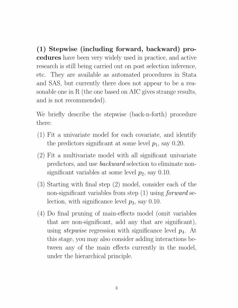
(1) Stepwise (including forward, backward) pro-

cedures have been very widely used in practice, and active

research is still being carried out on post selection inference,

etc. They are available as automated procedures in Stata

and SAS, but currently there does not appear to be a rea-

sonable one in R (the one based on AIC gives strange results,

and is not recommended).

We briefly describe the stepwise (back-n-forth) procedure

there:

(1) Fit a univariate model for each covariate, and identify

the predictors significant at some level p1, say 0.20.

(2) Fit a multivariate model with all significant univariate

predictors, and use backward selection to eliminate non-

significant variables at some level p2, say 0.10.

(3) Starting with final step (2) model, consider each of the

non-significant variables from step (1) using forward se-

lection, with significance level p3, say 0.10.

(4) Do final pruning of main-effects model (omit variables

that are non-significant, add any that are significant),

using stepwise regression with significance level p4. At

this stage, you may also consider adding interactions be-

tween any of the main effects currently in the model,

under the hierarchical principle.

3

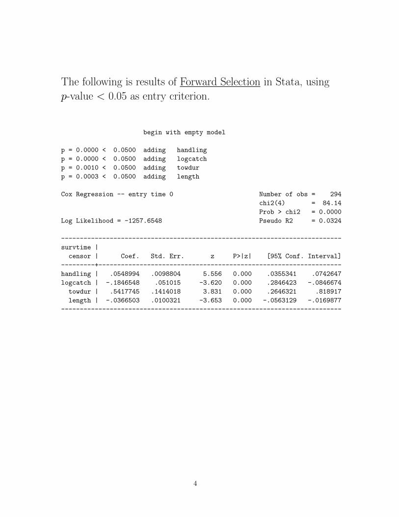
The following is results of Forward Selection in Stata, using

p-value < 0.05 as entry criterion.

begin with empty model

p = 0.0000 < 0.0500 adding handling

p = 0.0000 < 0.0500 adding logcatch

p = 0.0010 < 0.0500 adding towdur

p = 0.0003 < 0.0500 adding length

Cox Regression -- entry time 0 Number of obs = 294

chi2(4) = 84.14

Prob > chi2 = 0.0000

Log Likelihood = -1257.6548 Pseudo R2 = 0.0324

---------------------------------------------------------------------------

survtime |

censor | Coef. Std. Err. z P>|z| [95% Conf. Interval]

---------+-----------------------------------------------------------------

handling | .0548994 .0098804 5.556 0.000 .0355341 .0742647

logcatch | -.1846548 .051015 -3.620 0.000 .2846423 -.0846674

towdur | .5417745 .1414018 3.831 0.000 .2646321 .818917

length | -.0366503 .0100321 -3.653 0.000 -.0563129 -.0169877

---------------------------------------------------------------------------

4

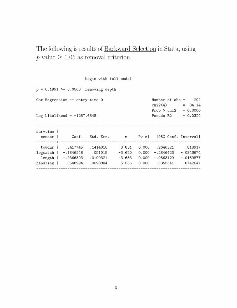
The following is results of Backward Selection in Stata, using

p-value ≥ 0.05 as removal criterion.

begin with full model

p = 0.1991 >= 0.0500 removing depth

Cox Regression -- entry time 0 Number of obs = 294

chi2(4) = 84.14

Prob > chi2 = 0.0000

Log Likelihood = -1257.6548 Pseudo R2 = 0.0324

--------------------------------------------------------------------------

survtime |

censor | Coef. Std. Err. z P>|z| [95% Conf. Interval]

---------+----------------------------------------------------------------

towdur | .5417745 .1414018 3.831 0.000 .2646321 .818917

logcatch | -.1846548 .051015 -3.620 0.000 -.2846423 -.0846674

length | -.0366503 .0100321 -3.653 0.000 -.0563129 -.0169877

handling | .0548994 .0098804 5.556 0.000 .0355341 .0742647

--------------------------------------------------------------------------

5

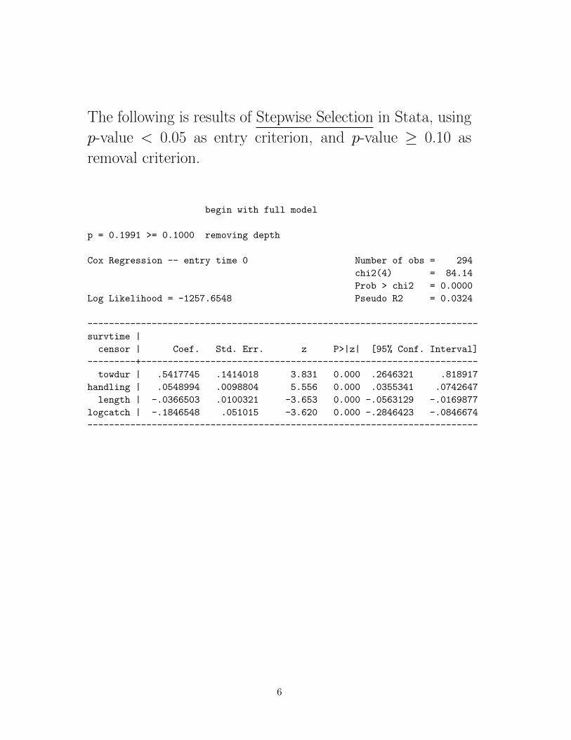
The following is results of Stepwise Selection in Stata, using

p-value < 0.05 as entry criterion, and p-value ≥ 0.10 as

removal criterion.

begin with full model

p = 0.1991 >= 0.1000 removing depth

Cox Regression -- entry time 0 Number of obs = 294

chi2(4) = 84.14

Prob > chi2 = 0.0000

Log Likelihood = -1257.6548 Pseudo R2 = 0.0324

-------------------------------------------------------------------------

survtime |

censor | Coef. Std. Err. z P>|z| [95% Conf. Interval]

---------+---------------------------------------------------------------

towdur | .5417745 .1414018 3.831 0.000 .2646321 .818917

handling | .0548994 .0098804 5.556 0.000 .0355341 .0742647

length | -.0366503 .0100321 -3.653 0.000 -.0563129 -.0169877

logcatch | -.1846548 .051015 -3.620 0.000 -.2846423 -.0846674

-------------------------------------------------------------------------

6

Notes:

• When the halibut data was analyzed with the forward,

backward and stepwise options, the same final model was

reached. However, this will not always be the case.

• Sometimes we want to force certain variables in the model

even if they may not be significant (lockterm option in

Stata and the include option in SAS).

• Depending on the software, different tests (Wald, score,

or likelihood ratio) may be used to decide what variables

to add and what variables to remove.

7

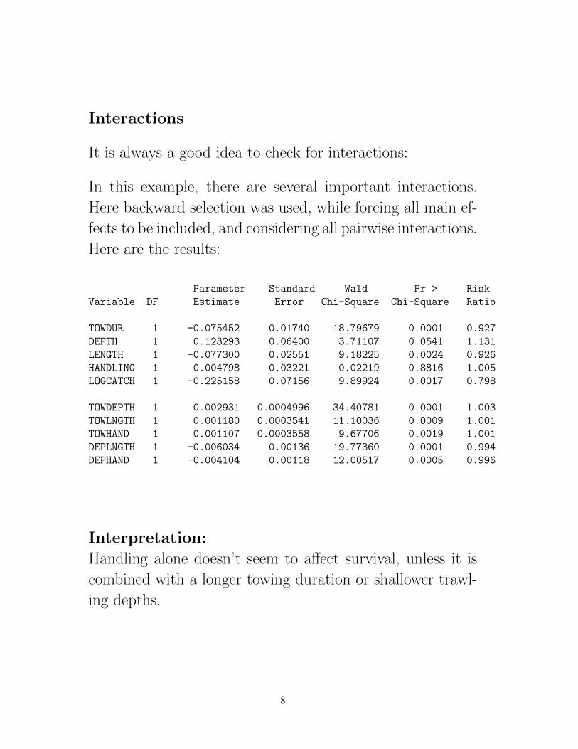
Interactions

It is always a good idea to check for interactions:

In this example, there are several important interactions.

Here backward selection was used, while forcing all main ef-

fects to be included, and considering all pairwise interactions.

Here are the results:

Parameter Standard Wald Pr > Risk

Variable DF Estimate Error Chi-Square Chi-Square Ratio

TOWDUR 1 -0.075452 0.01740 18.79679 0.0001 0.927

DEPTH 1 0.123293 0.06400 3.71107 0.0541 1.131

LENGTH 1 -0.077300 0.02551 9.18225 0.0024 0.926

HANDLING 1 0.004798 0.03221 0.02219 0.8816 1.005

LOGCATCH 1 -0.225158 0.07156 9.89924 0.0017 0.798

TOWDEPTH 1 0.002931 0.0004996 34.40781 0.0001 1.003

TOWLNGTH 1 0.001180 0.0003541 11.10036 0.0009 1.001

TOWHAND 1 0.001107 0.0003558 9.67706 0.0019 1.001

DEPLNGTH 1 -0.006034 0.00136 19.77360 0.0001 0.994

DEPHAND 1 -0.004104 0.00118 12.00517 0.0005 0.996

Interpretation:

Handling alone doesn’t seem to affect survival, unless it is

combined with a longer towing duration or shallower trawl-

ing depths.

8

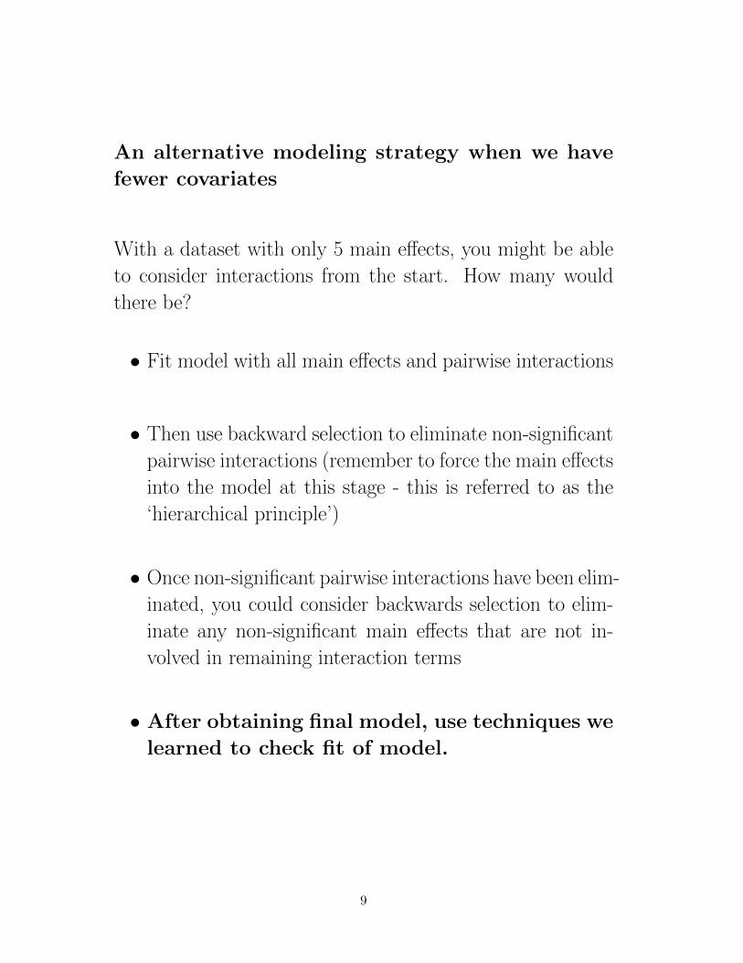
An alternative modeling strategy when we have

fewer covariates

With a dataset with only 5 main effects, you might be able

to consider interactions from the start. How many would

there be?

• Fit model with all main effects and pairwise interactions

• Then use backward selection to eliminate non-significant

pairwise interactions (remember to force the main effects

into the model at this stage - this is referred to as the

‘hierarchical principle’)

• Once non-significant pairwise interactions have been elim-

inated, you could consider backwards selection to elim-

inate any non-significant main effects that are not in-

volved in remaining interaction terms

• After obtaining final model, use techniques we

learned to check fit of model.

9

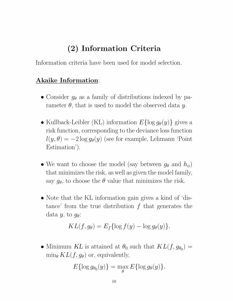
(2) Information Criteria

Information criteria have been used for model selection.

Akaike Information:

• Consider gθ as a family of distributions indexed by pa-

rameter θ, that is used to model the observed data y.

• Kullback-Leibler (KL) information Elog gθ(y) gives a

risk function, corresponding to the deviance loss function

l(y, θ) = −2 log gθ(y) (see for example, Lehmann ‘Point

Estimation’).

• We want to choose the model (say between gθ and hφ)

that minimizes the risk, as well as given the model family,

say gθ, to choose the θ value that minimizes the risk.

• Note that the KL information gain gives a kind of ‘dis-

tance’ from the true distribution f that generates the

data y, to gθ:

KL(f, gθ) = Eflog f (y)− log gθ(y).

• Minimum KL is attained at θ0 such that KL(f, gθ0) =

minθKL(f, gθ) or, equivalently,

Elog gθ0(y) = maxθElog gθ(y).

10

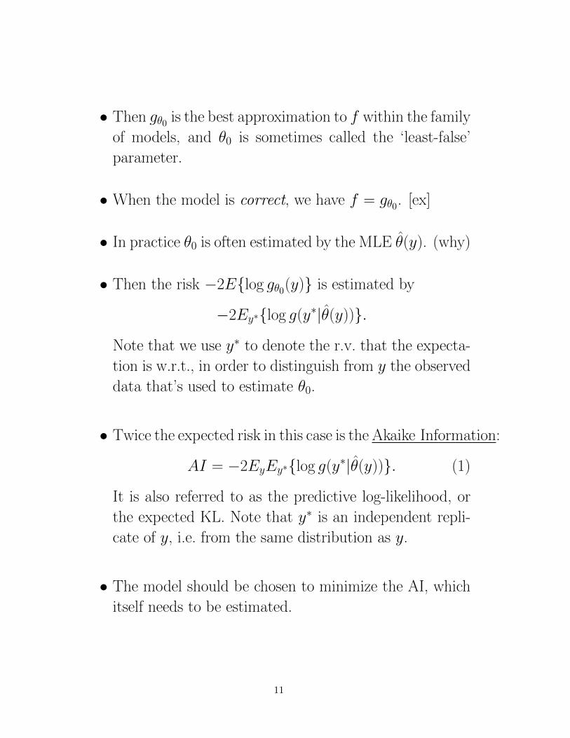
• Then gθ0 is the best approximation to f within the family

of models, and θ0 is sometimes called the ‘least-false’

parameter.

• When the model is correct, we have f = gθ0. [ex]

• In practice θ0 is often estimated by the MLE θ(y). (why)

• Then the risk −2Elog gθ0(y) is estimated by

−2Ey∗log g(y∗|θ(y)).

Note that we use y∗ to denote the r.v. that the expecta-

tion is w.r.t., in order to distinguish from y the observed

data that’s used to estimate θ0.

• Twice the expected risk in this case is the Akaike Information:

AI = −2EyEy∗log g(y∗|θ(y)). (1)

It is also referred to as the predictive log-likelihood, or

the expected KL. Note that y∗ is an independent repli-

cate of y, i.e. from the same distribution as y.

• The model should be chosen to minimize the AI, which

itself needs to be estimated.

11

• Q: how would you estimate AI?

• It is well-known that the ‘apparent’ estimate−2 log g(y|θ(y))

under-estimates AI. (why)

• Instead Akaike (1973) showed using asymptotic 2nd or-

der Taylor expansion that

AIC = −2 log g(y|θ(y)) + 2p (2)

is an approximately unbiased estimator of AI, where p

is the dimension of θ in the classical parametric case.

• Therefore the model is chosen to minimize the AIC.

12

AIC for the Cox Model

Since under the Cox model, λ0(t) is unspecified, model se-

lection focuses on the β part.

• It is perhaps intuitive that the partial likelihood should

be used in forming AIC.

• This turns out to be the case (Xu et al., 2009), because

the partial likelihood possesses the properties of a classi-

cal likelihood, especially in terms of the 2nd order Taylor

expansion that was used in the proof of classic AIC (re-

call partial likelihood as a profile likelihood).

• So

AIC = −2 pl(y|β(y)) + 2p,

where pl() is the log partial likelihood, and p is the di-

mension of β.

13

Interpretation

• In terms of the underlying KL information, since the par-

tial likelihood does not exactly correspond to a density

function, it has to be viewed via the profile likelihood.

• In this case, denote θ = (β, λ0), where β is the parameter

of interest, and λ0 is the nuisance parameter.

• Since λ0 is left unspecified, the relevant ‘distance’ is that

between the true distribution f and the subfamily of

models gβ,λ0 : λ0 ∈ Λ, which is: minλ0∈ΛKL(f, gβ,λ0).

• This is equivalent to

maxλ0

Elog gβ,λ0(y),

which in the empirical version corresponds to the profile

likelihood

pl(y|β) = maxλ0

log g(y|β, λ0).

• You can read more in Xu, Vaida and Harrington (2009)

about profile Akaike information.

14

BIC for the Cox Model

For classical parametric models, the Bayesian information

criterion is

BIC = −2 log g(y|θ(y)) + p · log(n), (3)

where n is the sample size.

For censored survival data, the number of events d, instead

of the number of subjects n, is the ‘effective’ sample size.

Note that d is the number of terms in the partial likelihood,

as well as the number of terms in the Fisher information.

Volinsky and Raftery (2000) proposed BIC for the Cox model:

BIC = −2 pl(y|β(y)) + p · log(d),

where d is the number of events.

15

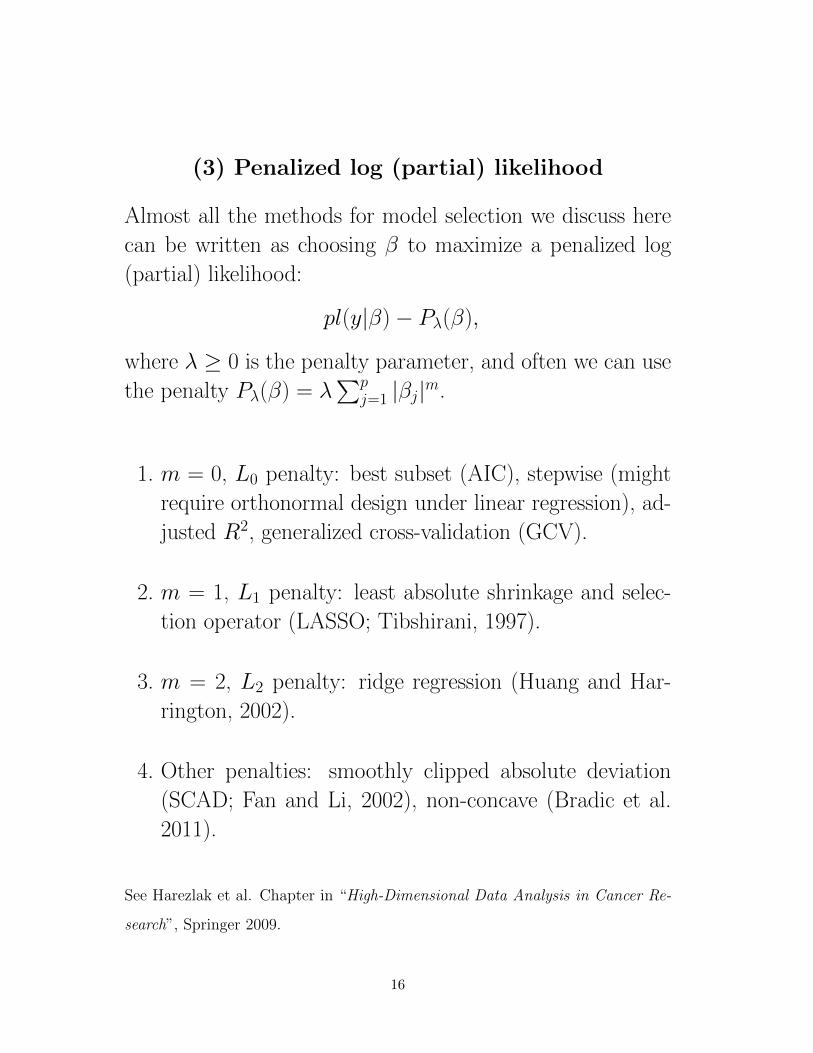
(3) Penalized log (partial) likelihood

Almost all the methods for model selection we discuss here

can be written as choosing β to maximize a penalized log

(partial) likelihood:

pl(y|β)− Pλ(β),

where λ ≥ 0 is the penalty parameter, and often we can use

the penalty Pλ(β) = λ∑p

j=1 |βj|m.

1. m = 0, L0 penalty: best subset (AIC), stepwise (might

require orthonormal design under linear regression), ad-

justed R2, generalized cross-validation (GCV).

2. m = 1, L1 penalty: least absolute shrinkage and selec-

tion operator (LASSO; Tibshirani, 1997).

3. m = 2, L2 penalty: ridge regression (Huang and Har-

rington, 2002).

4. Other penalties: smoothly clipped absolute deviation

(SCAD; Fan and Li, 2002), non-concave (Bradic et al.

2011).

See Harezlak et al. Chapter in “High-Dimensional Data Analysis in Cancer Re-

search”, Springer 2009.

16

(4) R2-type Measures

In a prognostic study in gastric cancer, we wanted to inves-

tigate the prognostic effects of acute phase reactant proteins

and stage on survival. The types of questions we were inter-

ested in:

1. How much of the variability in survival is explained?

2. How strong are the effects of certain prognostic variables

once others have been accounted for?

3. How much predictability is lost, if at all, when replacing

a continuously measured covariate by a binary coding?

4. In other areas (eg AIDS) with Z(t). How much of effect

is “captured” by surrogate?

As pointed out by Korn and Simon (1991), among others,

the R2 measure concerns explained variation, or predictive

capability, but not the goodness-of-fit of a model (which is

a common misunderstanding).

17

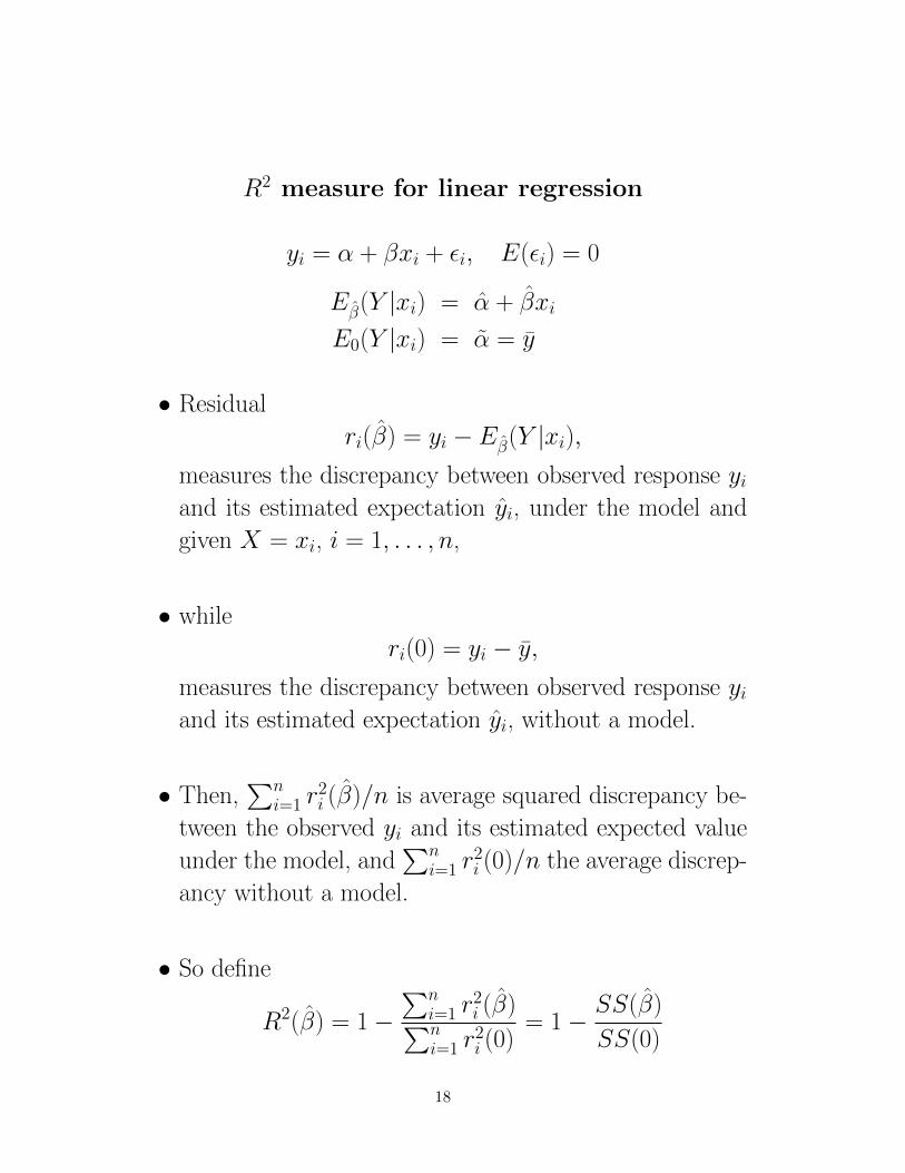
R2 measure for linear regression

yi = α + βxi + εi, E(εi) = 0

Eβ(Y |xi) = α + βxi

E0(Y |xi) = α = y

• Residual

ri(β) = yi − Eβ(Y |xi),measures the discrepancy between observed response yiand its estimated expectation yi, under the model and

given X = xi, i = 1, . . . , n,

• while

ri(0) = yi − y,measures the discrepancy between observed response yiand its estimated expectation yi, without a model.

• Then,∑n

i=1 r2i (β)/n is average squared discrepancy be-

tween the observed yi and its estimated expected value

under the model, and∑n

i=1 r2i (0)/n the average discrep-

ancy without a model.

• So define

R2(β) = 1−∑n

i=1 r2i (β)∑n

i=1 r2i (0)

= 1− SS(β)

SS(0)

18

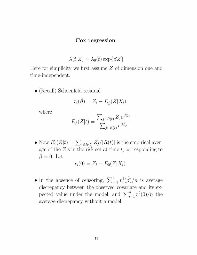
Cox regression

λ(t|Z) = λ0(t) expβZHere for simplicity we first assume Z of dimension one and

time-independent.

• (Recall) Schoenfeld residual

ri(β) = Zi − Eβ(Z|Xi),

where

Eβ(Z|t) =

∑j∈R(t)Zje

βZj∑j∈R(t) e

βZj

• Now E0(Z|t) =∑

j∈R(t)Zj/|R(t)| is the empirical aver-

age of the Z’s in the risk set at time t, corresponding to

β = 0. Let

ri(0) = Zi − E0(Z|Xi).

• In the absence of censoring,∑n

i=1 r2i (β)/n is average

discrepancy between the observed covariate and its ex-

pected value under the model, and∑n

i=1 r2i (0)/n the

average discrepancy without a model.

19

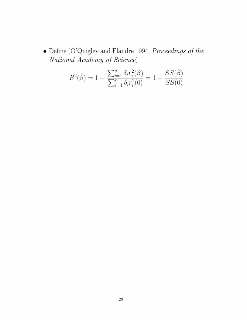
• Define (O’Quigley and Flandre 1994, Proceedings of the

National Academy of Science)

R2(β) = 1−∑n

i=1 δir2i (β)∑n

i=1 δir2i (0)

= 1− SS(β)

SS(0)

20

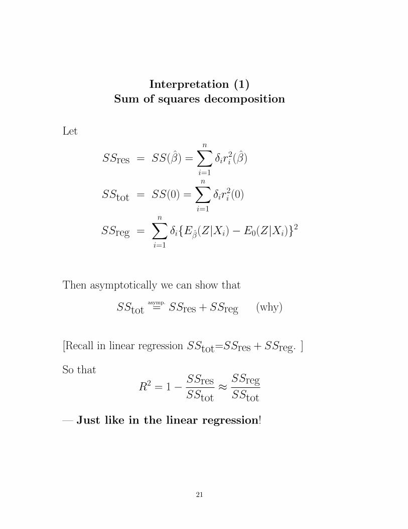
Interpretation (1)

Sum of squares decomposition

Let

SSres = SS(β) =

n∑i=1

δir2i (β)

SStot = SS(0) =

n∑i=1

δir2i (0)

SSreg =

n∑i=1

δiEβ(Z|Xi)− E0(Z|Xi)2

Then asymptotically we can show that

SStotasymp.= SSres + SSreg (why)

[Recall in linear regression SStot=SSres + SSreg. ]

So that

R2 = 1− SSresSStot

≈SSreg

SStot

— Just like in the linear regression!

21

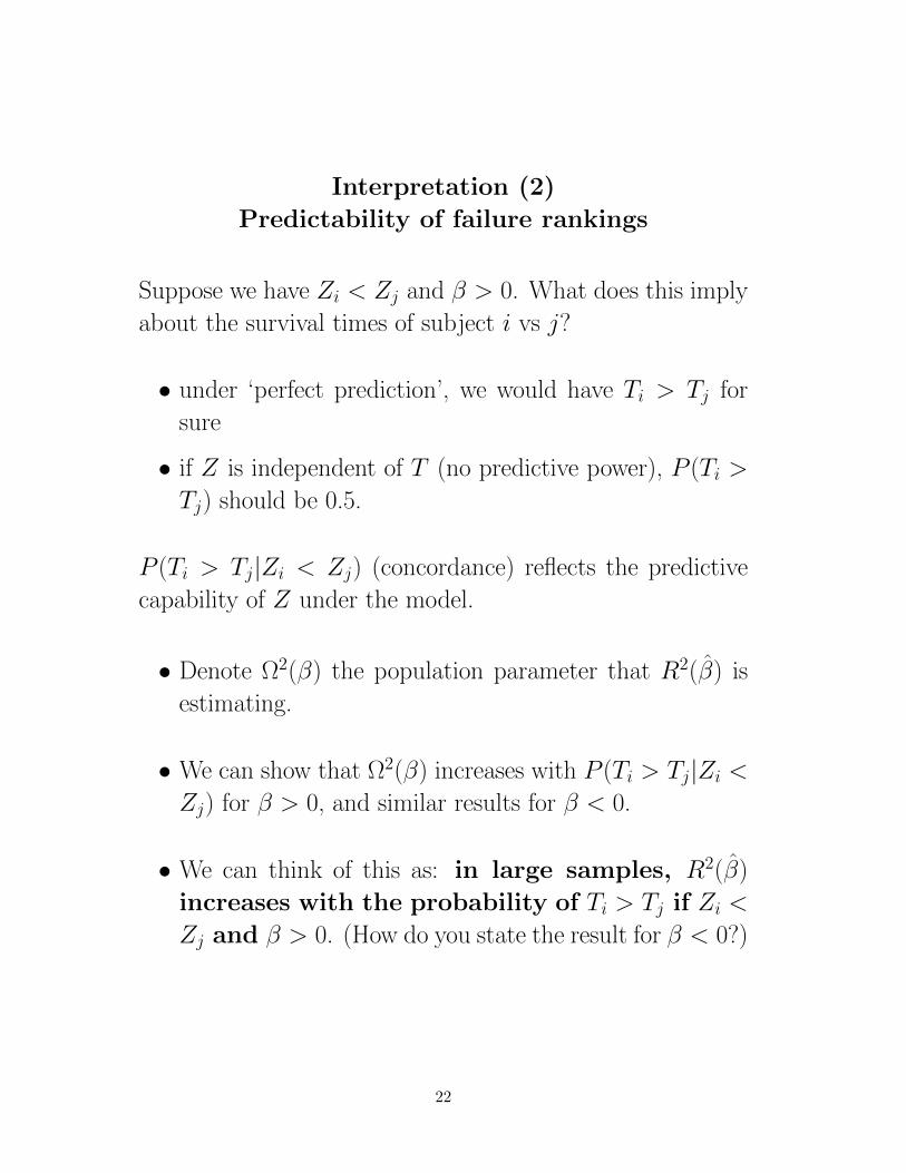
Interpretation (2)

Predictability of failure rankings

Suppose we have Zi < Zj and β > 0. What does this imply

about the survival times of subject i vs j?

• under ‘perfect prediction’, we would have Ti > Tj for

sure

• if Z is independent of T (no predictive power), P (Ti >

Tj) should be 0.5.

P (Ti > Tj|Zi < Zj) (concordance) reflects the predictive

capability of Z under the model.

• Denote Ω2(β) the population parameter that R2(β) is

estimating.

• We can show that Ω2(β) increases with P (Ti > Tj|Zi <Zj) for β > 0, and similar results for β < 0.

• We can think of this as: in large samples, R2(β)

increases with the probability of Ti > Tj if Zi <

Zj and β > 0. (How do you state the result for β < 0?)

22

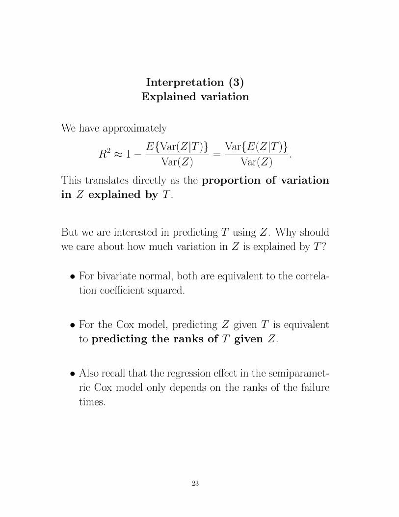
Interpretation (3)

Explained variation

We have approximately

R2 ≈ 1− EVar(Z|T )Var(Z)

=VarE(Z|T )

Var(Z).

This translates directly as the proportion of variation

in Z explained by T .

But we are interested in predicting T using Z. Why should

we care about how much variation in Z is explained by T ?

• For bivariate normal, both are equivalent to the correla-

tion coefficient squared.

• For the Cox model, predicting Z given T is equivalent

to predicting the ranks of T given Z.

• Also recall that the regression effect in the semiparamet-

ric Cox model only depends on the ranks of the failure

times.

23

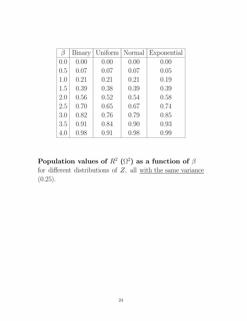
β Binary Uniform Normal Exponential

0.0 0.00 0.00 0.00 0.00

0.5 0.07 0.07 0.07 0.05

1.0 0.21 0.21 0.21 0.19

1.5 0.39 0.38 0.39 0.39

2.0 0.56 0.52 0.54 0.58

2.5 0.70 0.65 0.67 0.74

3.0 0.82 0.76 0.79 0.85

3.5 0.91 0.84 0.90 0.93

4.0 0.98 0.91 0.98 0.99

Population values of R2 (Ω2) as a function of β

for different distributions of Z, all with the same variance

(0.25).

24

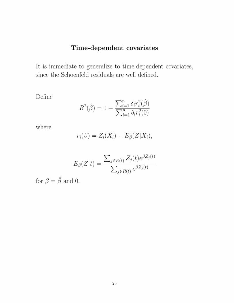
Time-dependent covariates

It is immediate to generalize to time-dependent covariates,

since the Schoenfeld residuals are well defined.

Define

R2(β) = 1−∑n

i=1 δir2i (β)∑n

i=1 δir2i (0)

where

ri(β) = Zi(Xi)− Eβ(Z|Xi),

Eβ(Z|t) =

∑j∈R(t)Zj(t)e

βZj(t)∑j∈R(t) e

βZj(t)

for β = β and 0.

25

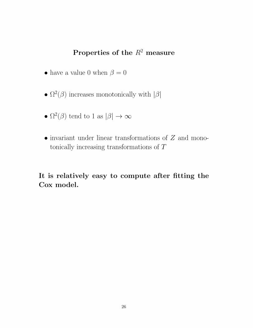
Properties of the R2 measure

• have a value 0 when β = 0

• Ω2(β) increases monotonically with |β|

• Ω2(β) tend to 1 as |β| → ∞

• invariant under linear transformations of Z and mono-

tonically increasing transformations of T

It is relatively easy to compute after fitting the

Cox model.

26

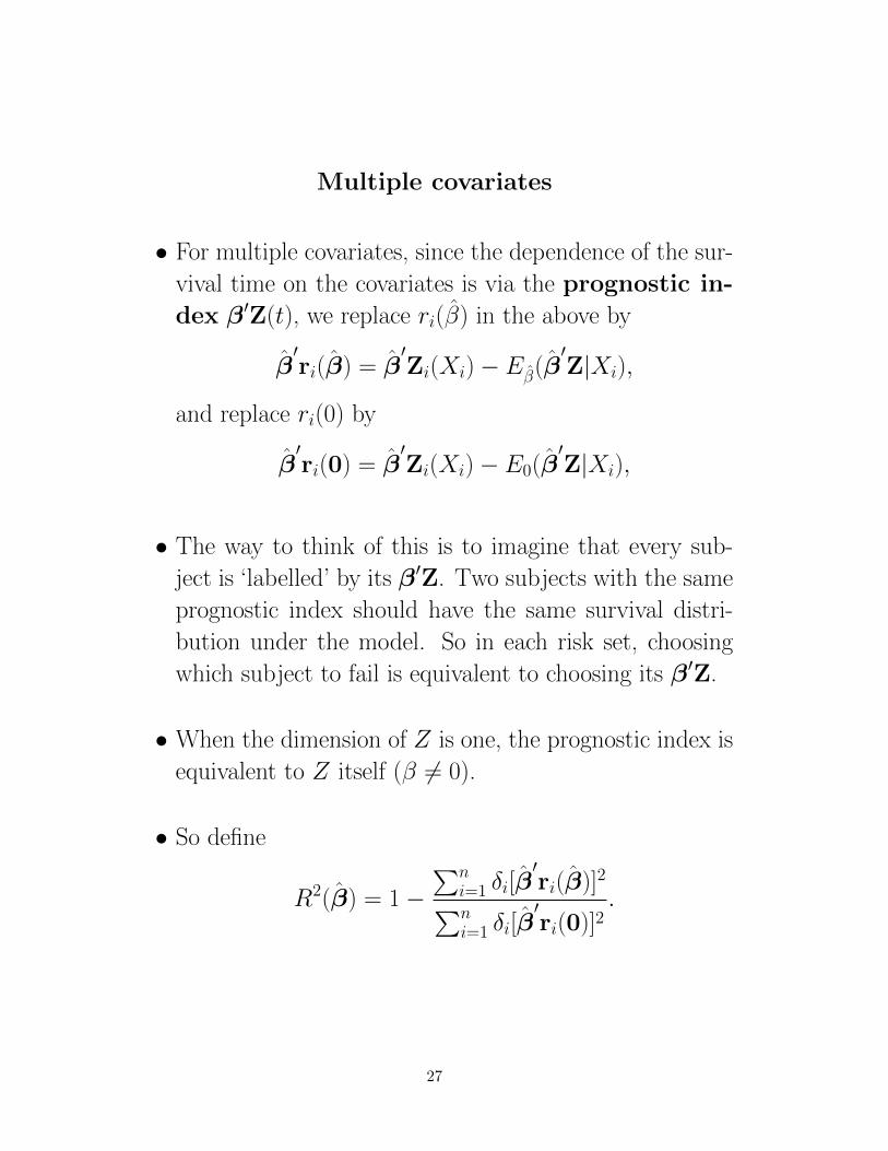
Multiple covariates

• For multiple covariates, since the dependence of the sur-

vival time on the covariates is via the prognostic in-

dex β′Z(t), we replace ri(β) in the above by

β′ri(β) = β

′Zi(Xi)− Eβ(β

′Z|Xi),

and replace ri(0) by

β′ri(0) = β

′Zi(Xi)− E0(β

′Z|Xi),

• The way to think of this is to imagine that every sub-

ject is ‘labelled’ by its β′Z. Two subjects with the same

prognostic index should have the same survival distri-

bution under the model. So in each risk set, choosing

which subject to fail is equivalent to choosing its β′Z.

• When the dimension of Z is one, the prognostic index is

equivalent to Z itself (β 6= 0).

• So define

R2(β) = 1−∑n

i=1 δi[β′ri(β)]2∑n

i=1 δi[β′ri(0)]2

.

27

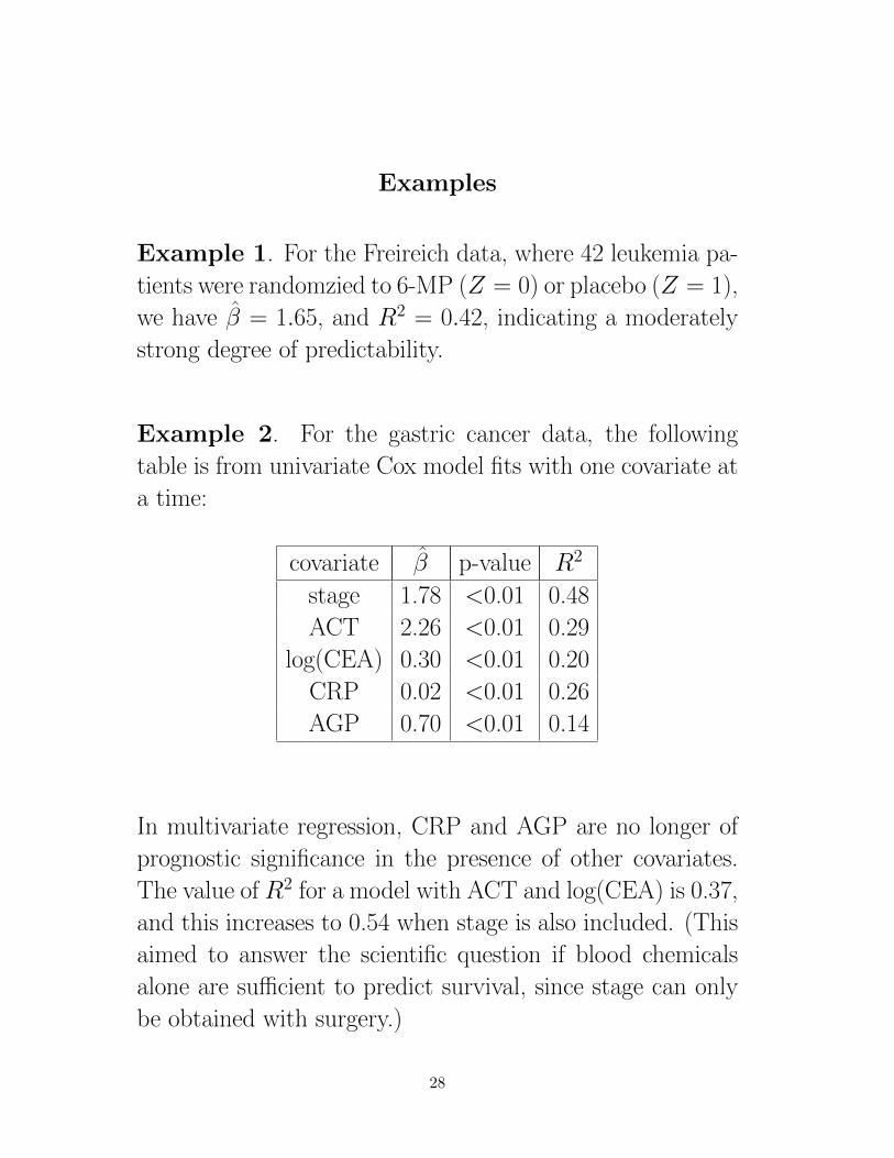
Examples

Example 1. For the Freireich data, where 42 leukemia pa-

tients were randomzied to 6-MP (Z = 0) or placebo (Z = 1),

we have β = 1.65, and R2 = 0.42, indicating a moderately

strong degree of predictability.

Example 2. For the gastric cancer data, the following

table is from univariate Cox model fits with one covariate at

a time:

covariate β p-value R2

stage 1.78 <0.01 0.48

ACT 2.26 <0.01 0.29

log(CEA) 0.30 <0.01 0.20

CRP 0.02 <0.01 0.26

AGP 0.70 <0.01 0.14

In multivariate regression, CRP and AGP are no longer of

prognostic significance in the presence of other covariates.

The value of R2 for a model with ACT and log(CEA) is 0.37,

and this increases to 0.54 when stage is also included. (This

aimed to answer the scientific question if blood chemicals

alone are sufficient to predict survival, since stage can only

be obtained with surgery.)

28

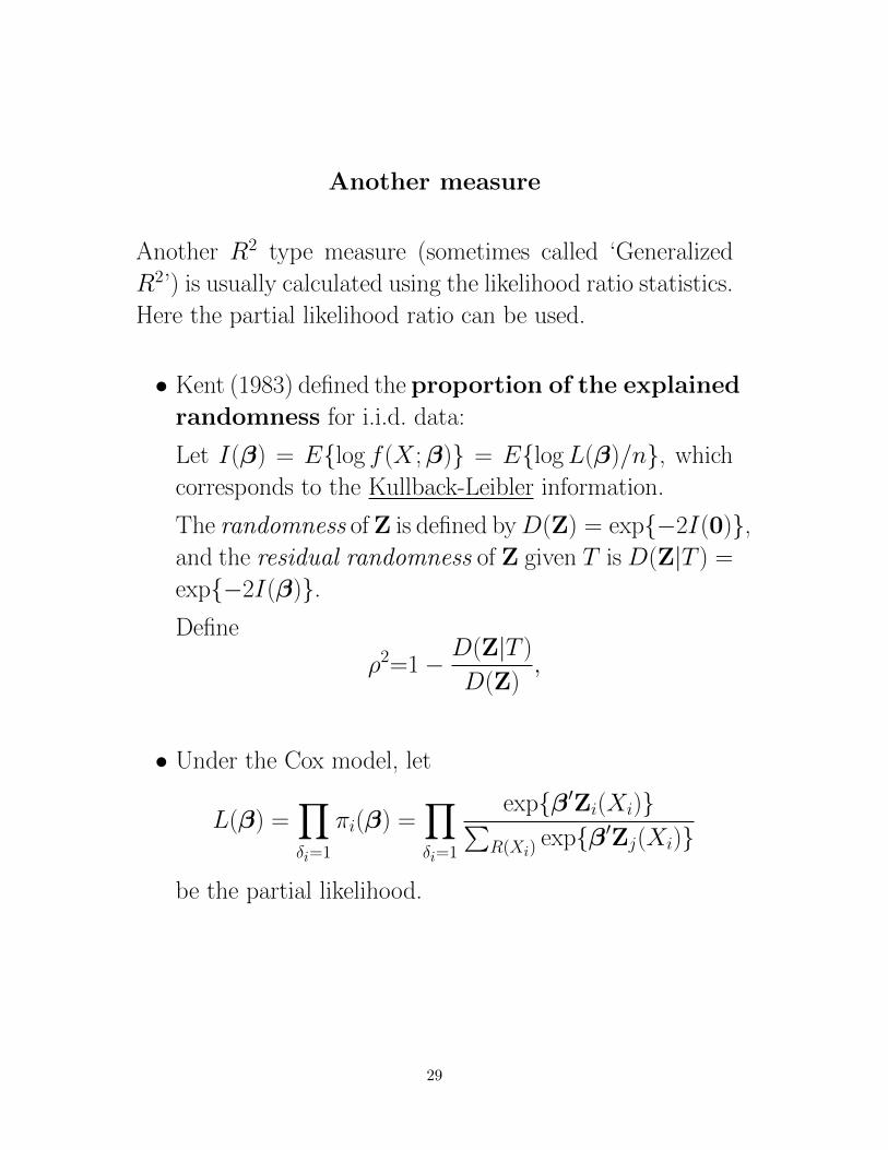
Another measure

Another R2 type measure (sometimes called ‘Generalized

R2’) is usually calculated using the likelihood ratio statistics.

Here the partial likelihood ratio can be used.

• Kent (1983) defined the proportion of the explained

randomness for i.i.d. data:

Let I(β) = Elog f (X ;β) = ElogL(β)/n, which

corresponds to the Kullback-Leibler information.

The randomness of Z is defined byD(Z) = exp−2I(0),and the residual randomness of Z given T is D(Z|T ) =

exp−2I(β).Define

ρ2=1− D(Z|T )

D(Z),

• Under the Cox model, let

L(β) =∏δi=1

πi(β) =∏δi=1

expβ′Zi(Xi)∑R(Xi)

expβ′Zj(Xi)

be the partial likelihood.

29

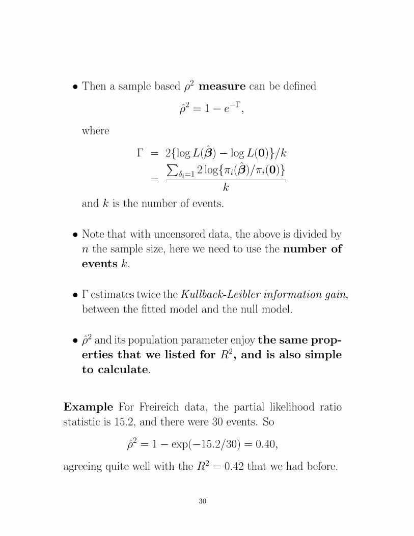
• Then a sample based ρ2 measure can be defined

ρ2 = 1− e−Γ,

where

Γ = 2logL(β)− logL(0)/k

=

∑δi=1 2 logπi(β)/πi(0)

k

and k is the number of events.

• Note that with uncensored data, the above is divided by

n the sample size, here we need to use the number of

events k.

• Γ estimates twice the Kullback-Leibler information gain,

between the fitted model and the null model.

• ρ2 and its population parameter enjoy the same prop-

erties that we listed for R2, and is also simple

to calculate.

Example For Freireich data, the partial likelihood ratio

statistic is 15.2, and there were 30 events. So

ρ2 = 1− exp(−15.2/30) = 0.40,

agreeing quite well with the R2 = 0.42 that we had before.

30

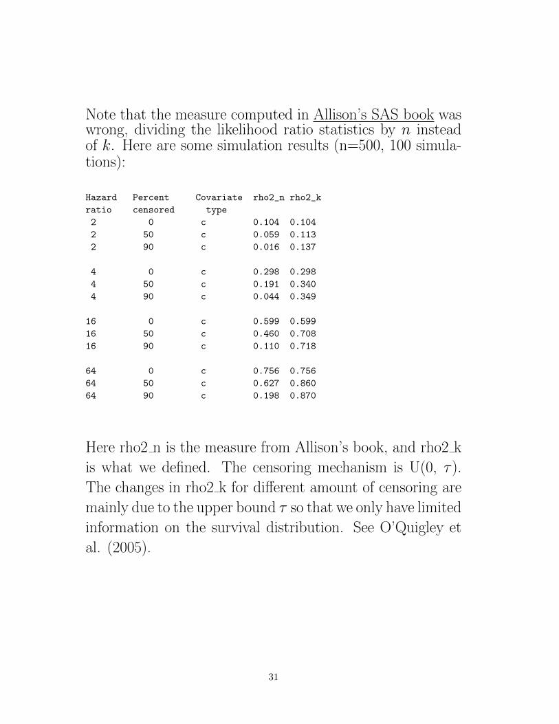
Note that the measure computed in Allison’s SAS book waswrong, dividing the likelihood ratio statistics by n insteadof k. Here are some simulation results (n=500, 100 simula-tions):

Hazard Percent Covariate rho2_n rho2_k

ratio censored type

2 0 c 0.104 0.104

2 50 c 0.059 0.113

2 90 c 0.016 0.137

4 0 c 0.298 0.298

4 50 c 0.191 0.340

4 90 c 0.044 0.349

16 0 c 0.599 0.599

16 50 c 0.460 0.708

16 90 c 0.110 0.718

64 0 c 0.756 0.756

64 50 c 0.627 0.860

64 90 c 0.198 0.870

Here rho2 n is the measure from Allison’s book, and rho2 k

is what we defined. The censoring mechanism is U(0, τ ).

The changes in rho2 k for different amount of censoring are

mainly due to the upper bound τ so that we only have limited

information on the survival distribution. See O’Quigley et

al. (2005).

31

Remarks

• In Handbook of Statistics in Clinical Oncology (ed.

Crowley), Chapter on ‘Explained variation in propor-

tional hazards regression’, it is argued that in the defi-

nition of R2, the squared Schoenfeld residuals should be

weighted to offset the censoring effect, and the weights

should be the increments of the marginal KM curve.

This will make the measure closer to the population

parameter Ω2. But for most practical purposes, both

versions give similar results.

• Following the same reasoning as above, the 2 logπi(β)/πi(0)’sin the definition of ρ2, instead of summing up and di-

viding by k, strictly speaking should also be weighted

proportionally to the increments of the marginal KM

curve. Again, in practice the two versions are similar, so

you may not have to compute the more complicated one

(O’Quigley et al., 2005).

• We saw some examples of R2 and ρ2 values. For cer-

tain data such as time-dependent CD4 counts, which of-

ten serves as a surrogate endpoint for survival in AIDS

studies, the explained variation/randomness in survival

by CD4 counts can be as high as over 80%.

32