Embed Size (px)
Citation preview

Model Theory Lecture Notes
Alex Kruckman
Updated: December 14, 2018
Contents
1 Syntax and semantics 21.1 Vocabularies . . . . . . . . . . . . . . . . . . . . . . . . . . . . . 31.2 S-indexed sets . . . . . . . . . . . . . . . . . . . . . . . . . . . . 51.3 Structures . . . . . . . . . . . . . . . . . . . . . . . . . . . . . . . 51.4 Terms and evaluation . . . . . . . . . . . . . . . . . . . . . . . . 71.5 Formulas and satisfaction . . . . . . . . . . . . . . . . . . . . . . 91.6 Theories and models . . . . . . . . . . . . . . . . . . . . . . . . . 11
2 Boolean algebras 122.1 Orders, lattices, Boolean algebras . . . . . . . . . . . . . . . . . . 122.2 Filters and ultrafilters . . . . . . . . . . . . . . . . . . . . . . . . 152.3 Stone duality . . . . . . . . . . . . . . . . . . . . . . . . . . . . . 17
3 Proofs and completeness for first-order logic 203.1 A proof system . . . . . . . . . . . . . . . . . . . . . . . . . . . . 203.2 Soundness and completeness . . . . . . . . . . . . . . . . . . . . . 243.3 First applications of compactness . . . . . . . . . . . . . . . . . . 31
4 Elementary embeddings 334.1 Homomorphisms and embeddings (again) . . . . . . . . . . . . . 334.2 Elementary equivalence and elementary embeddings . . . . . . . 344.3 Counting . . . . . . . . . . . . . . . . . . . . . . . . . . . . . . . 364.4 Boring and interesting theories . . . . . . . . . . . . . . . . . . . 384.5 The Lowenheim–Skolem theorems . . . . . . . . . . . . . . . . . 394.6 κ-categoricity and completeness . . . . . . . . . . . . . . . . . . . 41
5 Definability 465.1 Formulas and types . . . . . . . . . . . . . . . . . . . . . . . . . . 465.2 Syntactic classes of formulas and equivalence . . . . . . . . . . . 495.3 Up and down: ∃-formulas and ∀-formulas . . . . . . . . . . . . . 525.4 Directed colimits: ∀∃ formulas . . . . . . . . . . . . . . . . . . . 53
1
6 Quantifier elimination 586.1 Fraısse limits . . . . . . . . . . . . . . . . . . . . . . . . . . . . . 586.2 Quantifier elimination . . . . . . . . . . . . . . . . . . . . . . . . 686.3 Model completeness and model companions . . . . . . . . . . . . 74
7 Countable models 807.1 Saturated models . . . . . . . . . . . . . . . . . . . . . . . . . . . 817.2 Atomic models and omitting types . . . . . . . . . . . . . . . . . 837.3 ℵ0-categorical theories . . . . . . . . . . . . . . . . . . . . . . . . 907.4 The number of countable models . . . . . . . . . . . . . . . . . . 91
1 Syntax and semantics
Mathematical logic, broadly speaking, is the field of mathematics which is con-Tuesday 8/21cerned with the language we use to describe and reason about mathematicalobjects. That is, it highlights the distinction between syntax (the language)and semantics (the object itself). This may sound philosophical, but mathe-maticians constantly describe objects of interest by syntactic presentations, andthen reason about the object by manipulating the syntax, e.g. the descriptionof an algebraic variety as the locus of some system of polynomials, the coordi-natization of a manifold by explicit charts, the specification of a constructionor function by an algorithm, the presentation of a group by generators andrelations, or the description of a function as an infinite series.
There are many kinds of syntax in mathematics (as evidenced by the exam-ples just given), and there are many logical systems (or logics, for short). Oneof the most important is first-order logic1, which is the system we will study inthis course.
Like any logic, first-order logic has a proof theory and a model theory. Prooftheory is focused on syntax: systems for formal reasoning in the logic, andtheir properties. On the other hand, model theory is focused on semantics. Ourobjects of study are elementary classes (classes of mathematical structures whichcan be axiomatized by theories in first-order logic), and relationships betweenproperties of a first-order theory, its elementary class of models, and definabilitywithin these models.
Here, “mathematical structure” has a precise meaning: a structure is a set(or a family of sets), equipped with distinguished elements, operations, andrelations. From the names for these distinguished elements, operations, andrelations, we build up formulas of first-order logic (syntax), which correspondto new definable sets (and elements, operations, relations) in the structure (se-mantics). For example, the distinguished operations in an algebraically closed
1Why is first-order logic important? For practical reasons: it is fairly expressive, while alsoexhibiting a number of nice properties, like compactness and a good proof system, which wewill discuss in this class. And for foundational reasons: ZFC set theory, expressed in first-orderlogic, is the standard foundation for mathematics (but we will not discuss any foundationalissues in this class).
2

field include addition and multiplication; the class of algebraically closed fieldsis the class of models of a first-order theory ACF, and definable sets relative tothis theory are (Boolean combinations of) affine algebraic sets.
So model theory is very abstract, in that we study first-order theories andelementary classes in general, rather than any particular theory or class. But wewill often ground ourselves and obtain applications by specializing the generaltheory to particular examples.
In the first part of this course, we will define the language of first-order logicone piece at a time, looking first at a piece of syntax, and then the correspondingbit of semantics, as shown in the table below. Some of will probably seempedantic, since we will work at a high level of abstraction, but at the sametime the syntax is usually well-chosen to make the intended semantics seemclear. But we will conclude this part with a very non-trivial theorem: Godel’sCompleteness Theorem,2 which shows that the syntactic notion of provabilityin first-order logic is equivalent to the semantic notation of logical entailment.This is the only bit of proof theory we will do in this course; as an immediateconsequence, we get the purely model-theoretic Compactness Theorem, whichwill be one of our main tools going forward.
Syntax Semantics
Vocabularies StructuresTerms EvaluationFormulas SatisfactionTheories ModelsProvability (`) Entailment (|=)
1.1 Vocabularies
A first-order vocabulary V consists of:
1. A nonempty set S of sorts.
2. A set F of function symbols.3 Each function symbol f ∈ F has a type(s1, . . . , sn)→ s, where {s1, . . . , sn, s} ⊆ S. In the case n = 0, we call thefunction symbol a constant symbol of type s.
3. A set R of relation symbols. Each relation symbol R ∈ R has a type(s1, . . . , sn), where {s1, . . . , sn} ⊆ S. In the case n = 0, we call the relationsymbol a proposition symbol.
2Not to be confused with Godel’s Incompleteness Theorem!3We are purposefully vague about what counts as a symbol (or a sort, for that matter);
the name symbol is meant to suggest something that you could write down with a pencil onpaper, but we have no intention of formalizing this notion! In practice, real-world symbols onpaper can be encoded as mathematical objects (e.g. sets) in any way you like, and a symbolcan be any mathematical object. In particular, a vocabulary may be uncountably infinite.
3

In the case that S is a singleton {s}, we say that V is single-sorted.4 Inthis case, we typically do not name the single sort. The type of a functionsymbol f ∈ F is always (s, . . . , s)→ s, and the length of the tuple (s, . . . , s) iscalled the arity of f . Similarly, the type of a relation symbol R ∈ R is always(s, . . . , s), and the length of the tuple (s, . . . , s) is called the arity of R. Thewords unary, binary, and ternary mean arity 1, 2, and 3, respectively, andwe also write n-ary to mean arity n for n 6= 1, 2, 3. In the single-sorted setting,constant symbols are 0-ary function symbols, and proposition symbols are 0-aryrelation symbols.
When V is finite, it is often convenient to list it as
(s1, . . . , sl; f1, . . . , fm;R1, . . . , Rn).
It is to be understood from the notation that S = {s1, . . . , sl}, F = {f1, . . . , fm},and R = {R1, . . . , Rn}. The types of the function and relation symbols aresuppressed. In the single-sorted case, the single sort is usually omitted.
Example 1.1. We begin with an example which demonstrates the use of mul-tiple sorts. The vocabulary of vector spaces is:
(k, v; 0k, 1k,+k,×k,−k, 0v,+v,−v, ·).
• 0k and 1k are constant symbols of type k.
• +k and ×k are function symbols of type (k, k)→ k.
• −k is a function symbol of type k → k.
• 0v is a constant symbol of type v.
• +v is a function symbol of type (v, v)→ v.
• −v is a function symbol of type v → v.
• · is a function symbol of type (k, v)→ v.
This vocabulary can be extended in many ways, e.g. to the vocabulary of innerproduct spaces, obtained by adding a function symbol 〈−,−〉 of type (v, v)→ k.
Example 1.2. There are often multiple vocabularies which are appropriatefor a given kind of structure. Which one to use depends on the context. Forexample, if we are only interested in vector spaces over a fixed field K, it maybe more convenient to use the vocabulary of K-vector spaces. This vocabularyis single-sorted:
(0,+,−, (a)a∈K).
• 0 is a constant symbol.
4Classically, model theory was only concerned with single-sorted vocabularies, but thereare advantages to developing the foundations in a multi-sorted setting.
4

• + is a binary function symbol.
• − is a unary function symbol.
• a is a unary function symbol, for every element a ∈ K.
Example 1.3. The vocabulary of graphs is single-sorted, with a single binaryrelation symbol E. The vocabulary of orders is single-sorted with a single binaryrelation symbol ≤. Of course, these vocabularies only differ in the name we’vechosen for the unique binary relation symbol; we try to choose symbols whichare suggestive of the semantics we have in mind.
Example 1.4. We can also mix function symbols and relation symbols in thesame vocabulary. The vocabulary of ordered groups is single-sorted:
(e, ·,−1 ,≤).
Here e is a constant symbol, · is a binary function symbol, −1 is a unary functionsymbol, and ≤ is a binary relation symbol.
1.2 S-indexed sets
Given a nonempty set S, an S-indexed set is a family of sets (As)s∈S .If A = (As)s∈S and B = (Bs)s∈S are S-indexed sets, an S-indexed map
f : A → B is a family of maps (fs : As → Bs)s∈S . We say that f is injec-tive if each component fs is injective, and surjective if each component fs issurjective. We denote the set of S-indexed maps A→ B by BA.
For each tuple (s1, . . . , sn) from S, we define A(s1,...,sn) =∏ni=1Asi . In the
case n = 0, we have the empty product, which is a singleton set A() = {∗}. AnS-indexed map f : A→ B induces a map f(s1,...,sn) : A(s1,...,sn) → B(s1,...,sn) by
f(s1,...,sn)(a1, . . . , an) = (fs1(a1), . . . , fsn(an)).
Let A = (As)s∈S be an S-indexed set. The cardinality of A, denoted |A|,is just the cardinality of the disjoint union
⊔s∈S As.
All of the standard operations on sets can be extended to S-indexed sets,componentwise. For example, A ∪ B = (As ∪ Bs)s∈S , A ∩ B = (As ∩ Bs)s∈S ,A \B = (As \Bs)s∈S , and A×B = (As ×Bs)s∈S . We write A ⊆ B if As ⊆ Bsfor all s ∈ S.
1.3 Structures
Let V = (S;F ;R) be a vocabulary. A V-structure A consists of:
1. An S-indexed set (As)s∈S , called the domain of A, which we also denoteby A.5
5Contrary to the traditional approach, we allow empty sorts and empty structures: In anV-structure A, we may have As = ∅ for some sort s, or even for every sort s.
5
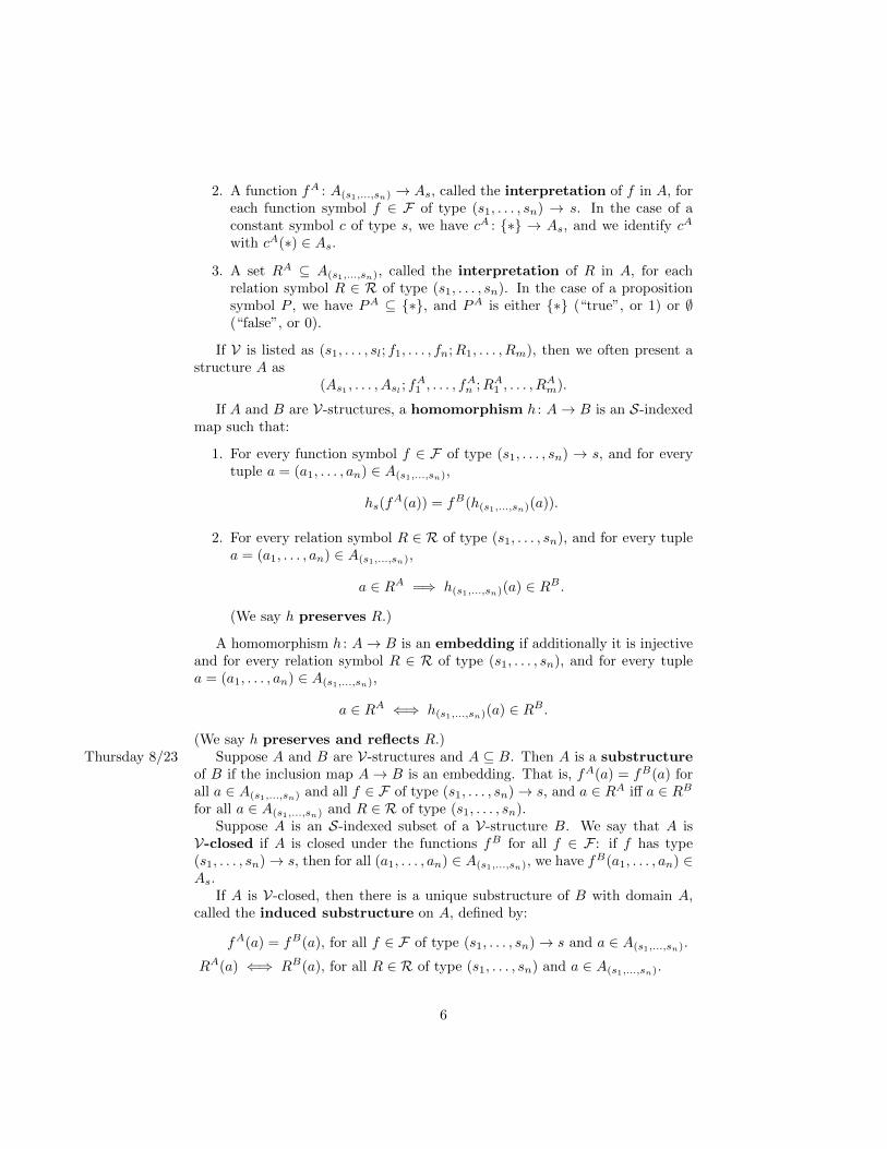
2. A function fA : A(s1,...,sn) → As, called the interpretation of f in A, foreach function symbol f ∈ F of type (s1, . . . , sn) → s. In the case of aconstant symbol c of type s, we have cA : {∗} → As, and we identify cA
with cA(∗) ∈ As.
3. A set RA ⊆ A(s1,...,sn), called the interpretation of R in A, for eachrelation symbol R ∈ R of type (s1, . . . , sn). In the case of a propositionsymbol P , we have PA ⊆ {∗}, and PA is either {∗} (“true”, or 1) or ∅(“false”, or 0).
If V is listed as (s1, . . . , sl; f1, . . . , fn;R1, . . . , Rm), then we often present astructure A as
(As1 , . . . , Asl ; fA1 , . . . , f
An ;RA1 , . . . , R
Am).
If A and B are V-structures, a homomorphism h : A→ B is an S-indexedmap such that:
1. For every function symbol f ∈ F of type (s1, . . . , sn) → s, and for everytuple a = (a1, . . . , an) ∈ A(s1,...,sn),
hs(fA(a)) = fB(h(s1,...,sn)(a)).
2. For every relation symbol R ∈ R of type (s1, . . . , sn), and for every tuplea = (a1, . . . , an) ∈ A(s1,...,sn),
a ∈ RA =⇒ h(s1,...,sn)(a) ∈ RB .
(We say h preserves R.)
A homomorphism h : A→ B is an embedding if additionally it is injectiveand for every relation symbol R ∈ R of type (s1, . . . , sn), and for every tuplea = (a1, . . . , an) ∈ A(s1,...,sn),
a ∈ RA ⇐⇒ h(s1,...,sn)(a) ∈ RB .
(We say h preserves and reflects R.)Suppose A and B are V-structures and A ⊆ B. Then A is a substructureThursday 8/23
of B if the inclusion map A→ B is an embedding. That is, fA(a) = fB(a) forall a ∈ A(s1,...,sn) and all f ∈ F of type (s1, . . . , sn)→ s, and a ∈ RA iff a ∈ RBfor all a ∈ A(s1,...,sn) and R ∈ R of type (s1, . . . , sn).
Suppose A is an S-indexed subset of a V-structure B. We say that A isV-closed if A is closed under the functions fB for all f ∈ F : if f has type(s1, . . . , sn)→ s, then for all (a1, . . . , an) ∈ A(s1,...,sn), we have fB(a1, . . . , an) ∈As.
If A is V-closed, then there is a unique substructure of B with domain A,called the induced substructure on A, defined by:
fA(a) = fB(a), for all f ∈ F of type (s1, . . . , sn)→ s and a ∈ A(s1,...,sn).
RA(a) ⇐⇒ RB(a), for all R ∈ R of type (s1, . . . , sn) and a ∈ A(s1,...,sn).
6

If A is an arbitrary S-indexed subset of a V-structure B, then the inducedsubstructure on the V-closure of A is the smallest substructure of B containingA. This is called the substructure generated by A and denoted 〈A〉.
An isomorphism is a homomorphism h : A → B such that there exists aninverse homomorphism h−1 : B → A. Equivalently, h is a surjective embedding.We write A ∼= B when A and B are isomorphic.
An automorphism of A is an isomorphism σ : A→ A. The automorphismsof A form a group under composition, denoted Aut(A). If C ⊆ A, we denote byAut(A/C) the subgroup of automorphisms of A fixing C pointwise:
Aut(A/C) = {σ ∈ Aut(A) | σs(c) = c for all c ∈ Cs}.
Later, we will meet other kinds of maps of interest between structures.
1.4 Terms and evaluation
Given the set S of sorts, we introduce an S-indexed set X = (Xs)s∈S of vari-ables. We will assume that the sets Xs are pairwise disjoint and countablyinfinite. The actual identity of the variables will not matter to us, so we willfeel free to use different names for them in different situations; the importantthing is that each variable has a fixed type s, and when we work with finitelymany variables at a time, we never run out of variables of any type.
A variable context is a finite tuple x = (x1, . . . , xk) of variables. If si isthe type of xi, we say the context has type (s1, . . . , sk). Note that there is anempty variable context (). We will abuse notation freely when concatenatingvariable contexts. For example, when x = (x1, . . . , xk) is a variable contextand y is another variable not in x, we write xy or x, y for the variable context(x1, . . . , xk, y).
A V-term of type s ∈ S in context x = (x1, . . . , xk) is one of the following:
• A variable xi of type s.
• A constant symbol c ∈ F of type s.
• A composite term f(t1, . . . , tn), where f ∈ F is a function symbol oftype (s1, . . . , sn) → s and ti is a V-term of type si in context x, for all1 ≤ i ≤ n.
Note that the case of constant symbols is really a special case of the case ofcomposite terms, when n = 0.
This is a definition by recursion (simultaneously across all types s), so weobtain a corresponding method of proof by induction. To prove a claim aboutall V-terms in context x, it suffices to check the base case (the claim holds forall variables in x), and the inductive step (given that the claim holds for theterms t1, . . . , tn, it holds for the composite term f(t1, . . . , tn)). Sometimes it isuseful to handle the constant symbols as a separate base case.
We denote by Ts(x) the set of V-terms of type s in context x, and by T (x) =(Ts(x))s∈S the S-indexed set of all V-terms in context x. We usually write t(x)to denote that the term t is in context x.
7
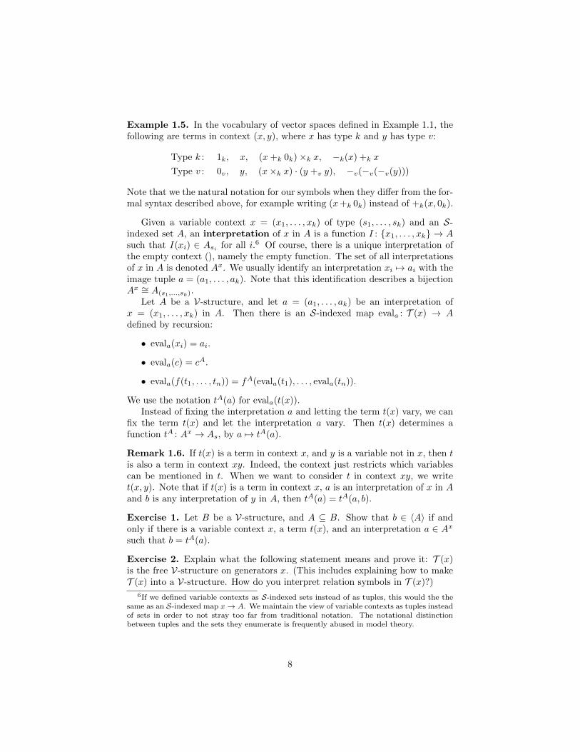
Example 1.5. In the vocabulary of vector spaces defined in Example 1.1, thefollowing are terms in context (x, y), where x has type k and y has type v:
Type k : 1k, x, (x+k 0k)×k x, −k(x) +k x
Type v : 0v, y, (x×k x) · (y +v y), −v(−v(−v(y)))
Note that we the natural notation for our symbols when they differ from the for-mal syntax described above, for example writing (x+k 0k) instead of +k(x, 0k).
Given a variable context x = (x1, . . . , xk) of type (s1, . . . , sk) and an S-indexed set A, an interpretation of x in A is a function I : {x1, . . . , xk} → Asuch that I(xi) ∈ Asi for all i.6 Of course, there is a unique interpretation ofthe empty context (), namely the empty function. The set of all interpretationsof x in A is denoted Ax. We usually identify an interpretation xi 7→ ai with theimage tuple a = (a1, . . . , ak). Note that this identification describes a bijectionAx ∼= A(s1,...,sk).
Let A be a V-structure, and let a = (a1, . . . , ak) be an interpretation ofx = (x1, . . . , xk) in A. Then there is an S-indexed map evala : T (x) → Adefined by recursion:
• evala(xi) = ai.
• evala(c) = cA.
• evala(f(t1, . . . , tn)) = fA(evala(t1), . . . , evala(tn)).
We use the notation tA(a) for evala(t(x)).Instead of fixing the interpretation a and letting the term t(x) vary, we can
fix the term t(x) and let the interpretation a vary. Then t(x) determines afunction tA : Ax → As, by a 7→ tA(a).
Remark 1.6. If t(x) is a term in context x, and y is a variable not in x, then tis also a term in context xy. Indeed, the context just restricts which variablescan be mentioned in t. When we want to consider t in context xy, we writet(x, y). Note that if t(x) is a term in context x, a is an interpretation of x in Aand b is any interpretation of y in A, then tA(a) = tA(a, b).
Exercise 1. Let B be a V-structure, and A ⊆ B. Show that b ∈ 〈A〉 if andonly if there is a variable context x, a term t(x), and an interpretation a ∈ Axsuch that b = tA(a).
Exercise 2. Explain what the following statement means and prove it: T (x)is the free V-structure on generators x. (This includes explaining how to makeT (x) into a V-structure. How do you interpret relation symbols in T (x)?)
6If we defined variable contexts as S-indexed sets instead of as tuples, this would the thesame as an S-indexed map x→ A. We maintain the view of variable contexts as tuples insteadof sets in order to not stray too far from traditional notation. The notational distinctionbetween tuples and the sets they enumerate is frequently abused in model theory.
8

1.5 Formulas and satisfaction
An atomic V-formula in context x is one of the following:
• (t1 = t2), where t1 and t2 are V-terms of type s in context x, for somes ∈ S.
• R(t1, . . . , tn), where R ∈ R is a relation symbol of type (s1, . . . , sn) andti is a V-term of type si in context x, for all 1 ≤ i ≤ n.
A V-formula in context x is one of the following:
• An atomic V-formula in context x.
• > or ⊥.
• (ψ ∧ χ), (ψ ∨ χ), or ¬ψ, where ψ and χ are V-formulas in context x.
• ∃y ψ, where y is a variable not in x and ψ is a V-formula in context xy.
This is a definition by recursion (simultaneously across all contexts x), so weobtain a corresponding method of proof by induction. To prove a claim aboutall V-formulas, it suffices to check the base case (the claim holds for all atomicformulas, >, and ⊥), and the inductive steps (given that the claim holds for theV-formulas ψ and χ, it holds for the formulas (ψ ∧ χ), (ψ ∨ χ), ¬ψ, and ∃y ψ).
We say that a variable y is bound in ϕ if some subformula of ϕ has theform ∃y ψ. Note that according to our definitions, if ϕ is in context x, then novariable in x can be bound in ϕ.
We will also employ the following standard shorthands:
• (t1 6= t2) is shorthand for ¬(t1 = t2).
• (ψ → χ) is shorthand for (¬ψ ∨ χ).
• (ψ ↔ χ) is shorthand for ((ψ → χ) ∧ (χ→ ψ)).
•∧ni=1 ϕi and
∨ni=1 ϕi are shorthand for (. . . ((ϕ1 ∧ ϕ2) ∧ ϕ3) · · · ∧ ϕn) and
(. . . ((ϕ1 ∨ ϕ2) ∨ ϕ3) · · · ∨ ϕn), respectively. In the case n = 0, the emptyconjunction is > and the empty disjunction is ⊥.
• ∀y ψ is shorthand for ¬∃y ¬ψ.7
We denote by Lx the set of all V-formulas in context x, and we usually writeϕ(x) to denote that the formula ϕ is in context x. We denote by L the setof all V-formulas, which is also called the first-order language correspondingto vocabulary V. When there is possibility for confusion, we can make thevocabulary explicit by writing L(V).
7It may seem perverse to define the universal quantifier in terms of the existential quantifier,but doing this has the advantage that we have fewer cases to check in proofs by induction onformulas. Of course, which logical connectives we take as primitive is a matter of convention.We could have similarly taken (ψ ∧ χ) as shorthand for ¬(¬ψ ∨¬χ), or done away with ∧, ∨,and ¬ altogether in favor of the Sheffer stroke ↑.
9

It is notationally common to begin a discussion by fixing a first-order lan-guage L, which is implicitly built from a vocabulary, which remains anonymous.Then we write things like L-structure and L-formula in place of V-structure andV-formula, where V is the vocabulary of L.8
Example 1.7. In the vocabulary of ordered groups defined in Example 1.4, thefollowing are formulas:
Context (x, y, z) : (x · y = e), (x ≤ y · z), ∃w (x · w ≤ z ∧ z ≤ y · w)
Empty context () : ∀xx · x−1 = e, ∃y (y 6= e ∧ ∀xx · y = y · x)
Note that we the natural notation for our symbols when they differ from theformal syntax described above, for example writing x ≤ y instead of ≤(x, y) andx−1 instead of −1(x).
Let A be a V-structure, let ϕ be a V-formula in context x, and let a be aninterpretation of x in A. We define the relation A |= ϕ(a), read A satisfiesϕ(a) or ϕ(a) is true in A, by induction on the structure of ϕ:
• If ϕ is (t1 = t2), then A |= ϕ(a) iff tA1 (a) = tA2 (a).
• If ϕ is R(t1, . . . , tn), then A |= ϕ(a) iff (tA1 (a), . . . , tAn (a)) ∈ RA.
• If ϕ is >, then A |= ϕ(a). If ϕ is ⊥, then A 6|= ϕ(a).
• If ϕ is (ψ ∧ χ), then A |= ϕ(a) iff A |= ψ(a) and A |= χ(a).
• If ϕ is (ψ ∨ χ), then A |= ϕ(a) iff A |= ψ(a) or A |= χ(a).
• If ϕ is ¬ψ, then A |= ϕ(a) iff A 6|= ψ(a).
• If ϕ is ∃y ψ, where y has type s, then A |= ϕ(a) iff there exists some b ∈ Assuch that A |= ψ(a, b).
As a consequence of these definitions, our shorthands also have their ex-pected meanings. For example:
• If ϕ is ψ → χ, then A |= ϕ iff A 6|= ψ or A |= χ, i.e. if A |= ψ, then A |= χ.
• If ϕ is ∀y ψ, where y has type s, then A |= ϕ iff there does not exist b ∈ Assuch that A 6|= ψ(a, b), i.e. for all b ∈ As, A |= ψ(a, b).
Remark 1.8. As in Remark 1.6, if ϕ(x) is a formula in context x, and y isa variable not in x and which is not bound in ϕ, then ϕ is also a formula incontext xy. When we want to consider ϕ in context xy, we write ϕ(x, y). Notethat if ϕ(x) is a formula in context x, a is an interpretation of x in A and b isany interpretation of y in A, then A |= ϕ(a) if and only if A |= ϕ(a, b).
Exercise 3. Prove the assertions in Remarks 1.6 and 1.8 by induction on thestructure of terms and formulas.
8In many sources, the distinction we have made between language and vocabulary isblurred, and only the term language is used.
10

1.6 Theories and models
A V-sentence ϕ is a V-formula in the empty context. When A is a V-structure,Tuesday 8/28there is a unique interpretation of the empty context in A. Then we write A |= ϕor A 6|= ϕ, without including the interpretation in the notation.
A V-theory T is a set of V-sentences. We write A |= T , read A satisfies Tor A is a model of T , if A |= ϕ for all ϕ ∈ T .
Let T be a theory, and let ϕ be a sentence. Then we write T |= ϕ, read Tentails ϕ, if every model of T satisfies ϕ. Of course, if ϕ ∈ T , then T |= ϕ byunraveling the definitions.
A theory T is complete if for every sentence ϕ, either T |= ϕ or T |= ¬ϕ.A theory T is satisfiable if T has a model. Note that T is satisfiable if and
only if T 6|= ⊥. Indeed, if T has a model A, then A 6|= ⊥, so T 6|= ⊥. On theother hand, if T has no models, then T |= ⊥ vacuously.
Example 1.9. Let A be any V-structure. Then the complete theory of A is
Th(A) = {ϕ ∈ L() | A |= ϕ}.
The name is justified, since for any sentence ϕ, either A |= ϕ or A 6|= ϕ. In thefirst case, ϕ ∈ Th(A), while in the second case A |= ¬ϕ, so ¬ϕ ∈ Th(A).
Example 1.10. Let V = (e, ·,−1 ) be the single-sorted vocabulary of groups.The theory Tgrp of groups consists of the following sentences:
∀x∀y∀z ((x · y) · z = x · (y · z))∀x ((x · e = x) ∧ (e · x = x))
∀x ((x · x−1 = e) ∧ (x−1 · x = e))
Of course, a V-structure is a group if and only if A |= Tgrp.The theory Tgrp is not complete. For example, if ϕ is the sentence
∀x∀y (x · y = y · x),
then T 6|= ϕ and T 6|= ¬ϕ, since there are both abelian and non-abelian groups.On the other hand, we have
Tgrp |= (∀x (x · x = e)→ ∀x∀y (x · y = y · x)),
since all groups of exponent 2 are abelian.
Given a theory T , how can we tell when T |= ϕ, or even when T is satisfiable?Well, we need to provide a proof. This can be an external proof, obtained by“ordinary mathematical” reasoning about the models of T (as in the previousexample). How easy this is depends on how well we understand the models of T .But it can also be useful to know that that is a robust notion of proof internal tofirst-order logic, obtained by directly manipulating the syntax, without thinkingabout models at all. Our goal is to define this notion of proof, denoted `, andshow that provability exactly captures entailment: T ` ϕ iff T |= ϕ.
As a warm-up, and to serve as firm footing from which to launch into com-pleteness for first-order logic, we will take a detour through the world of Booleanalgebras and propositional logic.
11

2 Boolean algebras
2.1 Orders, lattices, Boolean algebras
A preorder (X;�) is a set X together with a binary relation � on X such thatThursday 8/30for all x, y, z ∈ X:
• x � x.
• If x � y and y � z, then x � z.
A preorder is a partial order if it additionally satisfies:
• If x � y and y � x, then x = y.
If (X;�) is a preorder, then the relation x ∼ y iff x � y and y � x is anequivalence relation on X. We denote the equivalence class of x by [x]. Thequotient X/∼ comes equipped with a relation ≤, defined by [x] ≤ [y] if and onlyif x � y. Then (X/∼;≤) is a partial order.
A lattice is a partial order (X;≤) equipped with distinguished elements >(“top”) and ⊥ (“bottom”) and binary operations ∧ (“meet”) and ∨ (“join”)such that:
• > is the maximum element, i.e. for all x, x ≤ >.
• ⊥ is the minimum element, i.e. for all x, ⊥ ≤ x.
• x∧ y is the greatest lower bound of x and y, i.e. for all z, z ≤ x∧ y if andonly if z ≤ x and z ≤ y.
• x ∨ y is the least upper bound of x and y, i.e. for all z, x ∨ y ≤ z if andonly if x ≤ z and y ≤ z.
In a lattice, any finite set S = {x1, . . . , xn} has a greatest lower bound:∧S = (. . . ((x1 ∧ x2) ∧ x3) · · · ∧ xn),
and a least upper bound:∨S = (. . . ((x1 ∨ x2) ∨ x3) · · · ∨ xn).
The greatest lower bound of the empty set is >, and the least upper bound ofthe empty set is ⊥.
Example 2.1. Let A be any set. Then (P(A), A, ∅,∩,∪) is a lattice, called thepowerset lattice on A.
Now let A be a V-structure. Let Sub(A) be the set of all substructuresof A. Then Sub(A) forms a lattice, with top element > = A, bottom element⊥ = 〈∅〉, meet B∧C = B∩C, and join B∨C = 〈B∪C〉. When V is single-sortedand contains only relation symbols, then Sub(A) is isomorphic to the powersetlattice on A.
12

Exercise 4. Lattices also have a purely algebraic (or “equational”) definition,which doesn’t mention the order relation ≤. We’ll use the term algebraic latticefor this definition, to distinguish it from the previous definition.
An algebraic lattice is a set X equipped with distinguished elements >and ⊥ and binary operations ∧ and ∨ such that:
1. (X;∧,>) is a commutative idempotent monoid: for all x, y, z ∈ X,
(a) (x ∧ y) ∧ z = x ∧ (y ∧ z).(b) x ∧ > = > ∧ x = x.
(c) x ∧ y = y ∧ x(d) x ∧ x = x.
2. (X;∨,⊥) is a commutative idempotent monoid: for all x, y, z ∈ X,
(a) (x ∨ y) ∨ z = x ∨ (y ∨ z).(b) x ∨ ⊥ = ⊥ ∨ x = x.
(c) x ∨ y = y ∨ x.
(d) x ∨ x = x.
3. ∧ and ∨ satisfy the “absorption laws”: for all x, y ∈ X,
(a) x ∨ (x ∧ y) = x.
(b) x ∧ (x ∨ y) = x.
Show that if (X;≤,>,⊥,∧,∨) is a lattice, then (X;>,⊥,∧,∨) is an algebraiclattice. Conversely, show that if (X;>,⊥,∧,∨) is an algebraic lattice, then forall x, y ∈ X, we have x ∧ y = x iff x ∨ y = y. And if we define x ≤ y iff theseequivalent conditions hold, then (X;≤,>,⊥,∧,∨) is a lattice.
A distributive lattice is a lattice which satisfies the distributive law: forall x, y, z ∈ X,
x ∧ (y ∨ z) = (x ∧ y) ∨ (x ∧ z).
Exercise 5. Let X be a lattice. Show that X satisfies the distributive law ifand only if it satisfies the dual distributive law: for all x, y, z ∈ X,
x ∨ (y ∧ z) = (x ∨ y) ∧ (x ∨ z).
Example 2.2. The powerset lattice on any set is distributive. So is the sub-algebra lattice Sub(A) of any V-structure when the function symbols in V havearity at most 1, since in this case B ∨ C = 〈B ∪ C〉 = B ∪ C when B and Care substructures. But when V contains function symbols of arity at least 2,Sub(A) is typically not distributive.
13

If x is an element of a distributive lattice, then a complement of x is anelement y such that x ∧ y = ⊥ and x ∨ y = >.
A Boolean algebra is a distributive lattice equipped with an additionalunary operation ¬ (“complement”), such that ¬x is a complement of x.
It follows from Exercise 4 that we can also give a purely algebraic definitionof Boolean algebras, by adding the following axioms to the axioms listed there:
4. The distributive law: for all x, y, z ∈ X, x ∧ (y ∨ z) = (x ∧ y) ∨ (x ∧ z)
5. Complements: for all x ∈ X,
(a) x ∧ ¬x = ⊥.
(b) x ∨ ¬x = >.
Example 2.3. (a) Let A be a set. Then (P(A);⊆, A, ∅,∩,∪,−) is a Booleanalgebra. Here −B = A \B.
(b) Let A be an infinite set, and let P∗(A) = {B ⊆ A | B is finite, or cofinite}(B is cofinite if A \B is finite). Then (P∗(A);⊆, A, ∅,∩,∪,−) is a Booleanalgebra.
(c) Let X be a topological space. Then the family O(X) of open sets in X isnot naturally equipped with a Boolean algebra structure, since open setsare typically not closed under complement. But letting Cl(X) be the set ofclopen sets in X, (Cl(X);⊆, X, ∅,∩,∪,−) does form a Boolean algebra.
Later, we’ll see more examples of Boolean algebras which are not algebrasof sets under the standard set operations (∩, ∪, and −). But there is a goodreason for giving examples of this form: Stone duality tells us that every Booleanalgebra is isomorphic to a subalgebra of a powerset algebra. In fact, everyBoolean algebra is isomorphic to the algebra of clopen sets in a topologicalspace!
Exercise 6. Let X be a distributive lattice. Show that if y and z are bothcomplements of x, then y = z. So in a Boolean algebra, ¬x is the uniquecomplement of x.
Exercise 7. Let B be a Boolean algebra. Show that for all x, y ∈ B,
(a) ¬¬x = x.
(b) (De Morgan’s Laws) ¬(x ∧ y) = (¬x ∨ ¬y) and ¬(x ∨ y) = (¬x ∧ ¬y).
(c) ¬> = ⊥ and ¬⊥ = >.
(d) x ≤ y iff ¬y ≤ ¬x.
Exercise 8. Let B be a Boolean algebra. For any x, y ∈ B, we define
x→ y = ¬x ∨ yx↔ y = (x→ y) ∧ (y → x).
Show that x ≤ y iff x→ y = >, and x = y iff x↔ y = >.
14

2.2 Filters and ultrafilters
In this subsection, we fix a Boolean algebra B. A subset F ⊆ B is a filter if:
1. F is closed upwards: If x ∈ F and x ≤ y, then y ∈ F .
2. F is closed under finite meets: > ∈ F , and if x, y ∈ F , then x ∧ y ∈ F .
A filter F is proper if ⊥ /∈ F (equivalently, F ( B).Dually, a subset I ⊆ B is a ideal if:
1. I is closed downwards: If x ∈ I and y ≤ x, then y ∈ I.
2. I is closed under finite joints: ⊥ ∈ I, and if x, y ∈ I, then x ∨ y ∈ I.
It follows from Exercise 7 that if F is a filter, then ¬F = {¬x | x ∈ F} is anideal, and vice versa.
Let A be an arbitrary subset of B. Then we define:
Fil(A) = {x ∈ B |∧A′ ≤ x where A′ is a finite subset of A}.
We call Fil(A) the filter generated by A, a name which is justified by thefollowing lemma.
Lemma 2.4. Fil(A) is the smallest filter containing A.
Proof. If F is a filter containing A, then since F is closed under finite meets,∧A′ ∈ F for any finite A′ ⊆ A. And since F is closed upwards, x ∈ F for any
x ∈ Fil(A). So Fil(A) ⊆ F . It remains to show that Fil(A) is a filter.Closure upwards: If x ∈ Fil(A), and x ≤ y, then
∧A′ ≤ x ≤ y for some
finite A′ ⊆ A, so y ∈ Fil(A).Closure under finite meets: > ∈ Fil(A), since > =
∧∅. And if x, y ∈ F ,
witnessed by∧A1 ≤ x and
∧A2 ≤ y for finite A1, A2 ⊆ A, then∧
(A1 ∪A2) =∧A1 ∧
∧A2 ≤ x ∧ y,
so x ∧ y ∈ Fil(A).
An ultrafilter is a proper filter U such that x ∈ U or ¬x ∈ U for all x ∈ B.
Exercise 9. Let B be a Boolean algebra.
1. If f : B → B′ is a Boolean algebra homomorphism, then f−1({>B′}) ⊆ Bis a filter. We say that F is the kernel of f .
2. Conversely, if F is a filter, then there is Boolean algebra B/F and asurjective homomorphism πF : B → B/F such that F is the kernel of πF .We call B/F the quotient of B by F . Hint: Define an equivalencerelation ∼F on B by
x ∼F y iff (x↔ y) ∈ F.
15
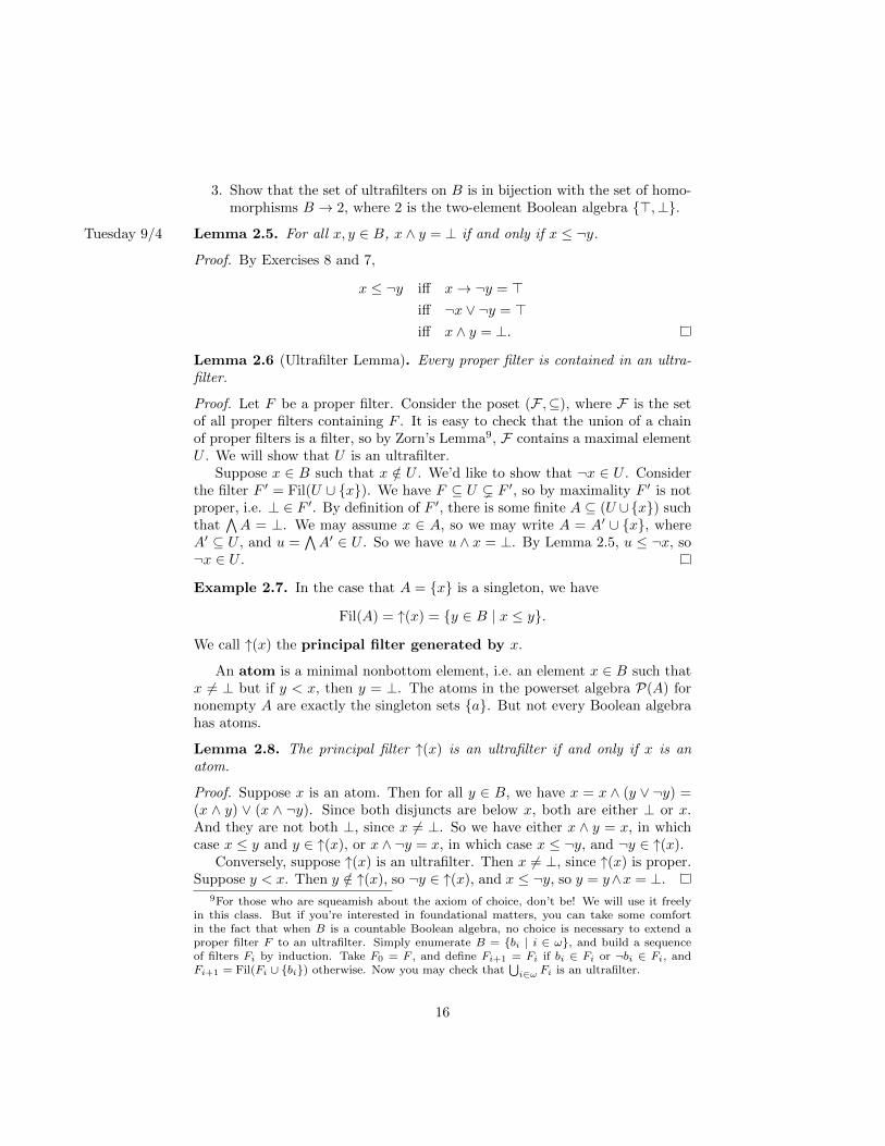
3. Show that the set of ultrafilters on B is in bijection with the set of homo-morphisms B → 2, where 2 is the two-element Boolean algebra {>,⊥}.
Lemma 2.5. For all x, y ∈ B, x ∧ y = ⊥ if and only if x ≤ ¬y.Tuesday 9/4
Proof. By Exercises 8 and 7,
x ≤ ¬y iff x→ ¬y = >iff ¬x ∨ ¬y = >iff x ∧ y = ⊥.
Lemma 2.6 (Ultrafilter Lemma). Every proper filter is contained in an ultra-filter.
Proof. Let F be a proper filter. Consider the poset (F ,⊆), where F is the setof all proper filters containing F . It is easy to check that the union of a chainof proper filters is a filter, so by Zorn’s Lemma9, F contains a maximal elementU . We will show that U is an ultrafilter.
Suppose x ∈ B such that x /∈ U . We’d like to show that ¬x ∈ U . Considerthe filter F ′ = Fil(U ∪ {x}). We have F ⊆ U ( F ′, so by maximality F ′ is notproper, i.e. ⊥ ∈ F ′. By definition of F ′, there is some finite A ⊆ (U ∪{x}) suchthat
∧A = ⊥. We may assume x ∈ A, so we may write A = A′ ∪ {x}, where
A′ ⊆ U , and u =∧A′ ∈ U . So we have u ∧ x = ⊥. By Lemma 2.5, u ≤ ¬x, so
¬x ∈ U .
Example 2.7. In the case that A = {x} is a singleton, we have
Fil(A) = ↑(x) = {y ∈ B | x ≤ y}.
We call ↑(x) the principal filter generated by x.
An atom is a minimal nonbottom element, i.e. an element x ∈ B such thatx 6= ⊥ but if y < x, then y = ⊥. The atoms in the powerset algebra P(A) fornonempty A are exactly the singleton sets {a}. But not every Boolean algebrahas atoms.
Lemma 2.8. The principal filter ↑(x) is an ultrafilter if and only if x is anatom.
Proof. Suppose x is an atom. Then for all y ∈ B, we have x = x ∧ (y ∨ ¬y) =(x ∧ y) ∨ (x ∧ ¬y). Since both disjuncts are below x, both are either ⊥ or x.And they are not both ⊥, since x 6= ⊥. So we have either x ∧ y = x, in whichcase x ≤ y and y ∈ ↑(x), or x ∧ ¬y = x, in which case x ≤ ¬y, and ¬y ∈ ↑(x).
Conversely, suppose ↑(x) is an ultrafilter. Then x 6= ⊥, since ↑(x) is proper.Suppose y < x. Then y /∈ ↑(x), so ¬y ∈ ↑(x), and x ≤ ¬y, so y = y∧x = ⊥.
9For those who are squeamish about the axiom of choice, don’t be! We will use it freelyin this class. But if you’re interested in foundational matters, you can take some comfortin the fact that when B is a countable Boolean algebra, no choice is necessary to extend aproper filter F to an ultrafilter. Simply enumerate B = {bi | i ∈ ω}, and build a sequenceof filters Fi by induction. Take F0 = F , and define Fi+1 = Fi if bi ∈ Fi or ¬bi ∈ Fi, andFi+1 = Fil(Fi ∪ {bi}) otherwise. Now you may check that
⋃i∈ω Fi is an ultrafilter.
16

Example 2.9. When the Boolean algebra B is a powerset algebra P(A), weabuse terminology by calling a filter U ⊆ P(A) a filter on A.
By Lemma 2.8, the principal filter ↑(X) = {Y ⊆ A | X ⊆ Y } for X ∈ P(A)is an ultrafilter if and only if |X| = 1. In this case, we call
↑({a}) = {Y ⊆ A | a ∈ Y }
the principal ultrafilter generated by a.When A is finite, every ultrafilter on A is principal. But when A is infinite,
there are non-principal ultrafilters on A. To see, this, define
C = {X ⊆ A | A \X is finite}.
This is called the cofinite filter or Frechet filter on A. When A is infinite,C is a proper filter, and by Lemma 2.6, C extends to an ultrafilter on A. ButC is not contained in the principal ultrafilter generated by a for any a ∈ A,since −{a} ∈ C. It should be noted that this proof really relies on the axiomof choice: it is impossible to write down any explicit example of a non-principalultrafilter on an infinite set A.
The situation is different for other Boolean algebras, of course. Recall theBoolean algebra P∗(A) from Example 2.3. In this algebra, the cofinite filter C(defined just as above) is already an ultrafilter.
2.3 Stone duality
Let B be a Boolean algebra. We define
S(B) = {U | U ⊆ B is an ultrafilter}.
For every element x ∈ B, let [x] = {U ∈ S(B) | x ∈ U}. So U ∈ [x] iff x ∈ U .This can be a bit confusing!
Lemma 2.10. For all x, y ∈ B,
(1) If x ≤ y, then [x] ⊆ [y].
(2) [>] = S(B) and [⊥] = ∅.
(3) [¬x] = S(B) \ [x].
(4) [x ∧ y] = [x] ∩ [y].
(5) [x ∨ y] = [x] ∪ [y].
Proof. (1) Suppose x ≤ y and U ∈ [x]. Then x ∈ U , so y ∈ U (U is closedupward), and U ∈ [y].
(2) Every ultrafilter on B contains > and no ultrafilter contains ⊥.
(3) ¬x ∈ U if and only if x /∈ U (U contains exactly one of x and ¬x).
17

(4) If U ∈ [x] ∩ [y], then x ∈ U and y ∈ U , so x ∧ y ∈ U (U is closed undermeets), and U ∈ [x∧ y]. Conversely, if U ∈ [x∧ y], then x∧ y ∈ U , so x ∈ Uand y ∈ U (U is closed upward), so U ∈ [x] ∩ [y].
(5) Using Exercise 7 and (3) and (4) above,
[x ∨ y] = [¬(¬x ∧ ¬y)]
= S(B) \ [¬x ∧ ¬y]
= S(B) \ ([¬x] ∩ [¬y])
= (S(B) \ [¬x]) ∪ (S(B) \ [¬y])
= [¬¬x] ∪ [¬¬y]
= [x] ∪ [y].
By conditions (2) and (4) of Lemma 2.10, the family {[x] | x ∈ B} containsS(B) and is closed under intersection, so it forms a basis for a topology τ onS(B). Note that each basic open set [x] is in fact clopen, since its complement[¬x] is also basic open.
A Stone space is a compact Hausdorff space with a basis of clopen sets.10
Lemma 2.11. The space S(B) is a Stone space.
Proof. We have already observed that S(B) has a basis of clopen sets. Forthe Hausdorff property, note that if U 6= V are points in S(B), then withoutloss of generality U 6⊆ V , so there is some x ∈ U with x /∈ V . Since V is anultrafilter, ¬x ∈ V . So [x] and [¬x] are disjoint open neighborhoods of U andV , respectively.
It remains to show compactness. We will prove the complemented form:Suppose (Ci)i∈I is a family of closed sets such that
⋂i∈I Ci = ∅. Then already
there is a finite subfamily (Ci)i∈J , where J is a finite subset of I, such that⋂i∈J Ci = ∅. Further, we may assume that each Ci is a basic clopen set, i.e.
[xi] for some xi ∈ B.Let F = Fil({xi | i ∈ I}). Suppose for contradiction that F is proper.
Then it extends to an ultrafilter U , and since {xi | i ∈ I} ⊆ F ⊆ U , we haveU ∈
⋂i∈I [xi] = ∅, contradiction. Thus F is not proper, and there is some J ⊆ I
such that∧i∈J xi = ⊥. Then [
∧i∈J xi] =
⋂i∈J [xi] = ∅.
We call S(B) the Stone space of B. Recall that when X is any topolog-ical space, the clopen algebra of X, (Cl(X);⊆, X, ∅,∩,∪,−), is the Booleanalgebra of clopen sets in X.
The Stone duality theorem says that every Boolean algebra is the clopenalgebra of some topological space (namely its Stone space), and every Stonespace is the Stone space of some Boolean algebra (namely its clopen algebra).
10Spaces with a basis of clopen sets are often called zero-dimensional ; the dimension inquestion is the small inductive dimension. It is a fact that a compact Hausdorff space iszero-dimensional if and only if it is totally disconnected, i.e. every connected component is asingleton. We will not prove that here.
18

Theorem 2.12 (Stone duality). For every Boolean algebra B, B ∼= Cl(S(B)).Thursday 9/6Conversely, for every Stone space X, X ∼= S(Cl(X)).
Proof. Let B be a Boolean algebra. Then the map [−] : B → Cl(S(B)) is definedby b 7→ [b]. Lemma 2.10 exactly says that [−] is a homomorphism. To see thatit is an embedding, it suffices to show that if [x] ⊆ [y], then x ≤ y. Indeed,injectivity follows, since if [x] = [y], then x ≤ y and y ≤ x, so x = y.
We show the contrapositive. So assume x 6≤ y. By Lemma 2.5, x ∧ ¬y 6= ⊥.So the filter ↑(x∧¬y) is proper and extends to an ultrafilter U . Now x∧¬y ∈ U ,so U ∈ [x] and U ∈ [¬y], so U /∈ [y]. It follows that [x] 6⊆ [y].
It remains to show that [−] is surjective. So let C ⊆ S(B) be a clopen set.Since C is open, we can write it as a union of basic open sets, C =
⋃i∈I [xi].
Since C is a closed subset of a compact space, it is compact, and the cover{[xi] | i ∈ I} has a finite subcover {[xi] | i ∈ J}, where J is a finite subset of I.Then C =
⋃i∈J [xi] = [
∨i∈J xi].
Conversely, let X be a Stone space. We will use several times the fact thatif p 6= q are points of X, then there is a clopen set C separating p and q, i.e.p ∈ C and q ∈ −C. Indeed, by Hausdorffness, p has an open neighborhood Vsuch that q /∈ V . By shrinking V , we may assume it is a basic clopen set.
The map f : X → S(Cl(X)) is given by p 7→ Up = {C ∈ Cl(X) | p ∈ C}.There are several things to check:
(a) Up is an ultrafilter. The clopen sets containing p are closed upward, closedunder intersection, include X, and do not include ∅. So Up is a proper filter.And for any clopen set C, either p ∈ C or p ∈ −C, so Ux is an ultrafilter.
(b) f is injective. If p 6= q, then letting C be a clopen set separating p and q,we have C ∈ Up and C /∈ Uq, so Up 6= Uq.
(c) f is surjective. Let U be an ultrafilter on Cl(X). Let P =⋂C∈U C. We
claim that P is a singleton {p} and f(p) = Up = U .
P is nonempty by compactness. Indeed, if⋂C∈U C = ∅, then there are
finitely many C1, . . . , Cn ∈ U such that⋂ni=1 Ci = ∅. But
⋂ni=1 Ci ∈ U ,
which is a contradiction.
If p, q ∈ P and the clopen set C separates p and q, then since either C or−C is in U , either p or q is not in P , contradiction. It follows that p and qare not separated, so p = q. Now it is clear that U ⊆ Up, since p ∈ C forall c ∈ U . And conversely, if p ∈ C, then −C /∈ U , so C ∈ U , and Up ⊆ U .
(d) f is continuous. A basic clopen set in S(Cl(X)) is of the form [C], where C isa clopen subset of X. We claim that f−1([C]) = C. Indeed, f(p) = Up ∈ [C]iff C ∈ Up iff p ∈ C.
(e) f is a homeomorphism. It suffices to show that the image of a closed setis closed. So let C ⊆ X be closed. Then C is compact (a closed subset ofa compact space is compact). So f(C) is compact (the continuous imageof a compact set is compact). So f(C) is closed (a compact subset of a
19

Hausdorff space is closed). What we have used here is just the general factthat a continuous bijection from a compact space to a Hausdorff space is ahomeomorphism.
As an immediate corollary, we get the following topology-free representationtheorem for Boolean algebras.
Corollary 2.13. Every Boolean algebra B embeds as a subalgebra of a powersetalgebra.
Proof. For any topological space X, the clopen algebra Cl(X) is a subalgebraof the powerset algebra P(X). So the Stone isomorphism B ∼= Cl(S(B)) is anembedding B ↪→ P(S(B)).
Exercise 10. (This exercise is not essential; you should only do it if you arealready comfortable with the language of category theory.)
1. Let Bool be the category of Boolean algebras and homomorphisms, and letStone be the category of Stone spaces and continuous maps. By definingtheir action on morphisms, show how to make S : Boolop → Stone andCl : Stoneop → Bool into contravariant functors between these categories.
2. Show that the pair (S,Cl) forms a contravariant equivalence of categoriesBool ≡ Stoneop. This is the modern formulation of the Stone dualitytheorem.
3. Let FinBool and FinSet be the categories of finite Boolean algebras andfinite sets, respectively. Show that FinBool is equivalent to FinSetop.
3 Proofs and completeness for first-order logic
3.1 A proof system
We now return to first-order logic and define the provability relation `. Ourproof rules are given below.11
11There are many sound and complete proof systems for first-order logic, i.e. many waysto define the relation `. The system presented here is definitely not the most efficient: interms of the number of rules, or from the point of view of proof theory. But I find it to bewell-motivated and well-suited for proving completeness.
20

Propositional rules: In these rules ϕ, χ, and ψ are formulas in context x.
ϕ `x ϕr
ϕ `x χ χ `x ψϕ `x ψ
t
ϕ `x >top
χ ∧ ψ `x χandL
χ ∧ ψ `x ψandR
ϕ `x χ ϕ `x ψϕ `x χ ∧ ψ
and
⊥ `x ϕbot
χ `x χ ∨ ψorL
ψ `x χ ∨ ψorR
χ `x ϕ ψ `x ϕχ ∨ ψ `x ϕ
or
ϕ ∧ (χ ∨ ψ) `x (ϕ ∧ χ) ∨ (ϕ ∧ ψ)d
ϕ ∧ ¬ϕ `x ⊥not1 > `x ϕ ∨ ¬ϕ
not2
Equality rules: In these rules, t, t′, and t′′ are terms of type s in contextx for some s ∈ S. Also, ti is a term of type si in context x for all 1 ≤ i ≤ n,f is a function symbol of type (s1, . . . , sn) → s, and R is a relation symbol oftype (s1, . . . , sn).
> `x t = tr=
t = t′ `x t′ = ts=
t = t′ ∧ t′ = t′′ `x t = t′′t=
∧ni=1 ti = t′i `x f(t1, . . . , tn) = f(t′1, . . . , t
′n)
fun
(∧ni=1 ti = t′i) ∧R(t1, . . . , tn) `x R(t′1, . . . , t
′n)
rel
Quantifier rules: In these rules, y is a single variable of type s not incontext x, t is a term of type s in context x, ϕ is a formula in context xy, andψ is a formula in context x in which y is not bound (so we an also view it as aformula in context xy).
ϕ[y 7→ t] `x ∃y ϕsub(t)
ϕ `xy ψ∃y ϕ `x ψ
e
In the rule (sub(t)), the notation ϕ[y 7→ t] means that the term t is sub-stituted for every instance of the variable y appearing in ϕ. Note that thissubstitution is only valid when y and t have the same type. If ϕ is a formulain context xy and t is a term in context x, then we view ϕ[y 7→ t] as a formulain context x. When we make the context explicit by writing the formula asϕ(x, y), we also write the new formula as ϕ(x, t).
The expression ϕ `x ψ is called a sequent. Notice that every sequent isdecorated by a variable context x, and that both formulas ϕ and ψ are in contextx. We just write ` instead of `() when the the context is empty.
21

In a rule, the sequents appearing above the horizontal line are the premises,and the sequent appearing below the horizontal line is the conclusion. A prooftree is a finite tree, with each node labeled by a sequent. A proof tree is valid iffor every node, there is some rule such that the node is labeled by the conclusion,and the children of the node are labeled by the premises, of an instance of thatrule. We assert ϕ ` ψ if this sequent labels the root of a valid proof tree.
Example 3.1. Let’s say our goal is to prove P ` ¬¬P , when P is a propositionalsymbol. The following is a valid proof tree:
P ` Pr
P ` >top
> ` ¬P ∨ ¬¬Pnot2
P ` ¬P ∨ ¬¬Pt
P ` P ∧ (¬P ∨ ¬¬P )and
P ∧ (¬P ∨ ¬¬P ) ` (P ∧ ¬P ) ∨ (P ∧ ¬¬P )d
P ` (P ∧ ¬P ) ∨ (P ∧ ¬¬P )t
Here is another one:
P ∧ ¬P ` ⊥not1 ⊥ ` P ∧ ¬¬P
bot
P ∧ ¬P ` P ∧ ¬¬Pt
P ∧ ¬¬P ` P ∧ ¬¬Pr
(P ∧ ¬P ) ∨ (P ∧ ¬¬P ) ` P ∧ ¬¬Por
P ∧ ¬¬P ` ¬¬PandR
(P ∧ ¬P ) ∨ (P ∧ ¬¬P ) ` ¬¬Pt
Putting these together yields P ` ¬¬P :
.
.
.
.P ` (P ∧ ¬P ) ∨ (P ∧ ¬¬P )
.
.
.
.(P ∧ ¬P ) ∨ (P ∧ ¬¬P ) ` ¬¬P
P ` ¬¬Pt
Example 3.2. Here is an example of tricky things you can do by shufflingvariables. Let x and y be single variables of the same type, let ϕ(y) be aformula in context y, and let ϕ′(x) be ϕ[y 7→ x], obtained by substituting x fory everywhere. The following proof tree shows that ∃xϕ′ ` ∃y ϕ.
ϕ′ `x ∃y ϕsub(x)
∃xϕ′ ` ∃y ϕe
In the first line, we view ∃y ϕ in the context x (although x is not mentioned inthis sentence). Since ϕ′ is ϕ[y 7→ x], this is a valid instance of (sub(x)). Thenwe can use (e) to introduce the quantifier and remove x from the context, sincex is not mentioned in ∃y ϕ.
We will make use of the fact that ∃xϕ′ ` ∃y ϕ in the proof of completeness.
Remark 3.3. The proof rules probably look familiar to you: they are essentiallyour axioms for Boolean algebras. Let’s make that precise.
Fix a variable context x, and recall that Lx is the set of all formulas incontext x. By (r) and (t), the relation ` is a preorder on Lx. We pass to the
associated partial order Lx, writing ϕ for the equivalence class of a sentence ϕ
22

(so ϕ = ψ if and only if ϕ ` ψ and ψ ` ϕ). We say that two sentences in thesame equivalence class are logically equivalent.
Now by (top) and (bot), this partial order has a top element > and a
bottom element ⊥. By (andL), (andR), and (and), χ ∧ ψ is the greatest lower
bound of χ and ψ, and by (orL), (orR), and (or), χ ∨ ψ is the least upper
bound of χ and ψ. So the partial order is a lattice, with meet and join as above.By (d), the lattice is distributive. There is something to be checked here,
since (d) only gives one inequality of the distributive law, namely
x ∧ (y ∨ z) ≤ (x ∧ y) ∨ (x ∧ z).
But the other inequality holds in any lattice. Indeed, note that x ∧ y ≤ x andx ∧ z ≤ x, so
(x ∧ y) ∨ (x ∧ z) ≤ x.Similarly, x ∧ y ≤ y ≤ y ∨ z, and x ∧ z ≤ z ≤ y ∨ z, so
(x ∧ y) ∨ (x ∧ z) ≤ y ∨ z.
It follows that(x ∧ y) ∨ (x ∧ z) ≤ x ∧ (y ∨ z).
Finally, by (not1) and (not2), every element ϕ has a complement ¬ϕ. So
Lx is a Boolean algebra.From this observation, we can already dispense with the hassle of construct-
ing explicit proof trees in many situations: for example, since the ` relationis the order relation on the Boolean algebra of sentences, syntactic ¬ is thecomplement operation in this Boolean algebra, and x = ¬¬x in any Booleanalgebra, we know that ϕ `x ¬¬ϕ, and also ¬¬ϕ `x ϕ, for any formula ϕ incontext x, without having to write out proof trees.
In the future, we will often dispense with the ϕ notation, identifying a for-mula with its logical equivalence class when there is no danger in doing so.
When T is a theory and ϕ is a sentence, we write T ` ϕ, read T proves ϕ,Tuesday 9/11if there are finitely many sentences ψ1, . . . ψn ∈ T such that
∧ni=1 ψi ` ϕ. We
say that T is inconsistent if T ` ⊥, and otherwise T is consistent.Note for any theory T , the set FT = {ϕ ∈ L() | T ` ϕ} of sentences provable
from T is exactly the filter generated by T in the Boolean algebra of sentences.This filter is proper if and only if T is consistent. And this filter is an ultrafilterif and only if T is complete (for provability), i.e. for every sentence ϕ, T ` ϕor T ` ¬ϕ. In the remainder of this section when we say T is complete, we meancomplete for provability. It will be a consequence of soundness and completenessthat a theory is complete for provability if and only if it is complete (as definedin Section 1.6 in terms of |=).
Lemma 3.4. Suppose T is a consistent theory. Then there is a complete theoryT ∗ such that T ⊆ T ∗.Proof. Since T is consistent, the associated filter FT = {ϕ ∈ L() | T ` ϕ} isproper. By the ultrafilter lemma, FT extends to an ultrafilter on L(), i.e. acomplete theory T ∗, and T ⊆ FT ⊆ T ∗.
23

3.2 Soundness and completeness
We now prove that the syntactic relation ` is equal to the semantic relation |=.
Theorem 3.5 (Soundness). If T ` ϕ, then T |= ϕ.
Proof. We say a sequent ϕ `x ψ is semantically valid if for every structure Aand every interpretation a of the context x, if A |= ϕ(a), then A |= ψ(a).
Claim: Every sequent which labels the root of a valid proof tree is seman-tically valid.
The argument is by induction on the complexity of the proof tree. In thebase case, we must show that for every rule with no premises, every instance ofthat rule is semantically valid. In the inductive step, for every instance of everyrule with premises, we may assume that the premises are semantically valid,and we must show that the conclusion is semantically valid.
There are many cases to check, but they are all straightforward. So we justillustrate a few for example. Consider the rule (and):
ϕ `x χ ϕ `x ψϕ `x χ ∧ ψ
and.
We may assume by induction that the premises are semantically valid. Let Abe a structure and a ∈ Ax such that A |= ϕ(a). By the induction hypothesis,A |= χ(a) and A |= ψ(a), so A |= (χ ∧ ψ)(a).
Consider the rule (rel):
(∧ni=1 ti = t′i) ∧R(t1, . . . , tn) `x R(t′1, . . . , t
′n)
rel
This is a base case. Let A be a structure and a ∈ Ax such that
A |= ((
n∧i=1
ti = t′i) ∧R(t1, . . . , tn))(a).
Then (tA1 (a), . . . , tAn (a)) ∈ RA. But also tAi (a) = (t′i)A(a) for all 1 ≤ i ≤ n, so
also ((t′1)A(a), . . . , (t′n)A(a)) ∈ RA, and A |= R(t′1, . . . , t′n)(a).
The quantifier rules are the most complicated, so we illustrate both of them.
ϕ[y 7→ t] `x ∃y ϕsub(t)
Let A be a structure and a ∈ Ax such that A |= ϕ[y 7→ t](a). That is,writing ϕ as ϕ(x, y), we have A |= ϕ(a, tA(a)). So A |= ∃y ϕ(a, y), witnessed bythe element tA(a).
ϕ `xy ψ∃y ϕ `x ψ
e
We may assume by induction that ϕ `xy ψ is semantically valid. Let A bea structure and a ∈ Ax such that A |= ∃y ϕ(a, y). Then there is some b ∈ As
24

such that A |= ϕ(a, b). By the induction hypothesis, A |= ψ(a, b), but ψ(x) is aformula in context x (it does not mention the variable y), so A |= ψ(a).
Having established the claim, assume T ` ϕ. Then there is a finite subsetΣ ⊆fin T such that
∧ψ∈Σ ψ ` ϕ. By the claim, every model of
∧ψ∈Σ ψ satisfies
ϕ. And since every model of T is a model of∧ψ∈Σ ψ, we have T |= ϕ.
So soundness just amounts to checking that the proof rules don’t say any-thing wrong. We now embark on proving the converse, completeness, which ismuch more involved.
We first prove an a priori weaker claim: Any consistent theory has a model.In other words, if T 6` ⊥, then T 6|= ⊥. How can we take a syntactic assumption,the consistency of T , and produce an actual model of T? We take a cue fromthe theory of free algebraic structures (e.g. free groups or the “term algebra”from Exercise 2) and construct the model from the syntax of T .
Construction 3.6. Let T be any V-theory. For each sort s ∈ S, recall that Tsis the set of V-terms of type s in the empty context. Define a relation ∼T on Tsby t ∼T t′ if and only if T ` (t = t′).
By (r=), (s=), and (t=), ∼T is an equivalence relation on Ts. We denote by[t] the equivalence class of t.
Let M(T )s = Ts/∼T . We will define a V-structure M(T ) with domain(M(T )s)s∈S .
For each function symbol f of type (s1, . . . , sn)→ s, define
fM ([t1], . . . , [tn]) = [f(t1, . . . , tn)].
This is well-defined: if ti ∼T t′i for 1 ≤ i ≤ n, then T |=∧ni=1 ti = t′i, so by
(fun), T |= f(t1, . . . , tn) = f(t′1, . . . , t′n), and f(t1, . . . , tn) ∼T f(t′1, . . . , t
′n).
For each relation symbol R of type (S1, . . . , Sn), define
([t1], . . . , [tn]) ∈ RM ⇐⇒ T ` R(t1, . . . , tn).
This is well-defined: if ti ∼T t′i for 1 ≤ i ≤ n and T ` R(t1, . . . , tn), thenT |= (
∧ni=1 ti = t′i) ∧R(t1, . . . , tn), so by (rel), T |= R(t′1, . . . , t
′n).
Our equality rules ensure that the V-structure M(T ) is well-defined, butwe’d really like it to be a model of T . The problem is that T might containa sentence with a quantifier, like ∃xϕ(x), and there is no guarantee that thereis a term t in the empty context such that M(T ) |= ϕ(t). In fact, if V has noconstant symbols, then there are no V-terms in the empty context at all, andM(T ) is empty! The following definition rectifies this situation.
A theory T has Henkin witnesses if for any formula ϕ(y) in a context witha single variable y of type s, if T ` ∃y ϕ(y), then there is a constant symbol cϕof type s such that T ` ϕ(cϕ).
Lemma 3.7. Suppose T is a complete consistent theory with Henkin witnesses.Then M(T ) |= T .
25
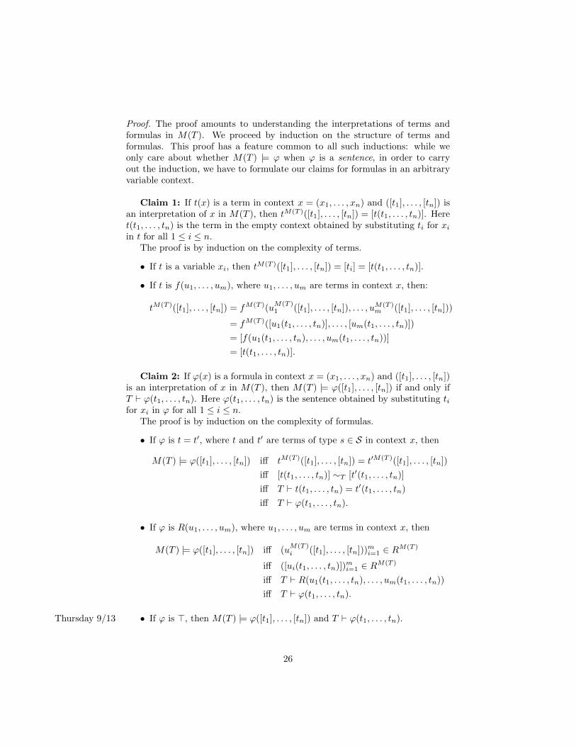
Proof. The proof amounts to understanding the interpretations of terms andformulas in M(T ). We proceed by induction on the structure of terms andformulas. This proof has a feature common to all such inductions: while weonly care about whether M(T ) |= ϕ when ϕ is a sentence, in order to carryout the induction, we have to formulate our claims for formulas in an arbitraryvariable context.
Claim 1: If t(x) is a term in context x = (x1, . . . , xn) and ([t1], . . . , [tn]) isan interpretation of x in M(T ), then tM(T )([t1], . . . , [tn]) = [t(t1, . . . , tn)]. Heret(t1, . . . , tn) is the term in the empty context obtained by substituting ti for xiin t for all 1 ≤ i ≤ n.
The proof is by induction on the complexity of terms.
• If t is a variable xi, then tM(T )([t1], . . . , [tn]) = [ti] = [t(t1, . . . , tn)].
• If t is f(u1, . . . , um), where u1, . . . , um are terms in context x, then:
tM(T )([t1], . . . , [tn]) = fM(T )(uM(T )1 ([t1], . . . , [tn]), . . . , uM(T )
m ([t1], . . . , [tn]))
= fM(T )([u1(t1, . . . , tn)], . . . , [um(t1, . . . , tn)])
= [f(u1(t1, . . . , tn), . . . , um(t1, . . . , tn))]
= [t(t1, . . . , tn)].
Claim 2: If ϕ(x) is a formula in context x = (x1, . . . , xn) and ([t1], . . . , [tn])is an interpretation of x in M(T ), then M(T ) |= ϕ([t1], . . . , [tn]) if and only ifT ` ϕ(t1, . . . , tn). Here ϕ(t1, . . . , tn) is the sentence obtained by substituting tifor xi in ϕ for all 1 ≤ i ≤ n.
The proof is by induction on the complexity of formulas.
• If ϕ is t = t′, where t and t′ are terms of type s ∈ S in context x, then
M(T ) |= ϕ([t1], . . . , [tn]) iff tM(T )([t1], . . . , [tn]) = t′M(T )([t1], . . . , [tn])
iff [t(t1, . . . , tn)] ∼T [t′(t1, . . . , tn)]
iff T ` t(t1, . . . , tn) = t′(t1, . . . , tn)
iff T ` ϕ(t1, . . . , tn).
• If ϕ is R(u1, . . . , um), where u1, . . . , um are terms in context x, then
M(T ) |= ϕ([t1], . . . , [tn]) iff (uM(T )i ([t1], . . . , [tn]))mi=1 ∈ RM(T )
iff ([ui(t1, . . . , tn)])mi=1 ∈ RM(T )
iff T ` R(u1(t1, . . . , tn), . . . , um(t1, . . . , tn))
iff T ` ϕ(t1, . . . , tn).
• If ϕ is >, then M(T ) |= ϕ([t1], . . . , [tn]) and T ` ϕ(t1, . . . , tn).Thursday 9/13
26

• If ϕ is ⊥, then M(T ) 6|= ϕ([t1], . . . , [tn]) and T 6` ϕ(t1, . . . , tn), since T isconsistent.
• If ϕ is χ ∧ ψ, then
M(T ) |= ϕ([t1], . . . , [tn]) iff M(T ) |= χ([t1], . . . , [tn])
and M(T ) |= ψ([t1], . . . , [tn])
iff T ` χ(t1, . . . , tn) and T ` ψ(t1, . . . , tn)
iff T ` ϕ(t1, . . . , tn).
• If ϕ is χ ∨ ψ, then
M(T ) |= ϕ([t1], . . . , [tn]) iff M(T ) |= χ([t1], . . . , [tn])
or M(T ) |= ψ([t1], . . . , [tn])
iff T ` χ(t1, . . . , tn) or T ` ψ(t1, . . . , tn)
iff T ` ϕ(t1, . . . , tn).
Here we used completeness: recall (from Lemma 2.10) that an ultrafiltercontains a join x ∨ y if and only if it contains x or it contains y.
• If ϕ is ¬χ, then
M(T ) |= ϕ([t1], . . . , [tn]) iff M(T ) 6|= χ([t1], . . . , [tn])
iff T 6` χ(t1, . . . , tn)
iff T ` ϕ(t1, . . . , tn),
since T is complete.
• If ϕ is ∃y ψ(x, y), suppose M(T ) |= ϕ([t1], . . . , [tn]). Then there is some[u] ∈ M(T )y such that M(T ) |= ψ([t1], . . . , [tn], [u]). By induction, T `ψ(t1, . . . , tn, u). By (sub(u)), T ` ∃y ψ(t1, . . . , tn, y), so T ` ϕ(t1, . . . , tn).
Conversely, suppose T ` ϕ(t1, . . . , tn). So T ` ∃y ψ(t1, . . . , tn, y). Let θ(y)be ψ(t1, . . . , tn, y). Since T has Henkin witnesses, T ` ψ(t1, . . . , tn, cθ).By induction, M(T ) |= ψ([t1], . . . , [tn], [cθ]), so M(T ) |= ϕ([t1], . . . , [tn]).
Now for every sentence ϕ ∈ T , we have T ` ϕ, so M(T ) |= ϕ by Claim 2.So M(T ) |= T , as was to be shown.
Of course, not every theory has Henkin witnesses. So our next goal is to takean arbitrary V-theory T and extend it to a complete V ′-theory T ′ with Henkinwitnesses, where V ′ is a vocabulary obtained by adding new constant symbolsto V. It is in this step where we need to do some real proof-theoretic work, sowe pause to make some observations about our proof system.
(1) Which instances of the rule (sub(t)) are available to us depends on thevocabulary. For example, if y is a variable of type s, the sentence ∃y> is
27

true in a structure if and only if the sort s is nonempty. If V has a term tof type s in the empty context (for example, a constant symbol of type s),then we have > ` ∃x> by (sub(t)), since >[x 7→ t] = >.
The sequent > ` ∃x> is semantically valid, since sort s is nonempty inevery V-structure (it contains at least the interpretation of the term t). Onthe other hand, if V has no terms of sort s in the empty context, then thereare V-structures in which the sort s is empty, and > 6` ∃x>.
Note that the term t does not actually appear in the proof tree for > ` ∃x>,just in the rule! This is why we make t explicit when writing (sub(t)). Whenwe say that a symbol or a variable occurs in a proof tree, we mean that itappears in any of the sentences in the sequents in the tree, or in a term tused in an instance of (sub(t)). When there could be any confusion aboutwhich vocabulary a proof takes place in, we will be careful to specify it.
(2) If ϕ `x ψ in vocabulary V, and V ⊆ V ′, then also ϕ `x ψ in vocabularyV ′. In the other direction, a proof in vocabulary V is a finite tree, and eachinstance of a rule uses only finitely many symbols in V, so if ϕ `x ψ, thenthere is a finite vocabulary V ′ ⊆ V (finitely many sorts, function symbols,and relation symbols) such that ϕ `x ψ in vocabulary V ′.
(3) Given a valid proof tree, a variable y which occurs in the tree, and a variabley′ of the same type which does not occur in the tree, we can replace y byy′ everywhere in the tree, and the resulting tree is still valid. This can bechecked by examining each rule and noting that replacing y by y′ results inan instance of the same rule.
(4) By Exercise 7, if ϕ `x ψ, then ¬ψ `x ¬ϕ. We will use this contrapositivetrick in applications of the rule (e). Specifically, suppose ϕ is a formulain context xy and ψ is a formula in context x in which y is not bound. Ifψ `xy ¬ϕ, then ψ `x ¬∃y ϕ.
Proof: If ψ `xy ¬ϕ, then ϕ `xy ¬ψ. By (e), ∃y ϕ `x ¬ψ, so ψ `x ¬∃y ϕ.
Lemma 3.8 (Lifting constants). Suppose V ′ = V ∪ {c}, where c is a constantsymbol of type s. Let ϕ and ψ be V ′-formulas in context x such that ϕ `x ψ.Let z be a variable of type s which is not in the context x and does not appearbound in ϕ or ψ. Then ϕ[c 7→ z] `xz ψ[c 7→ z] via a proof in the vocabulary V.
Proof. By point (3) above, we may assume that z does not occur in the prooftree for ϕ `x ψ. Then we can check, rule by rule, that if we replace the constantsymbol c by the variable z (which does not occur in the rule) and add z tothe contexts of all terms and formulas in the premises and conclusions, we getanother instance of the same rule in vocabulary V.
The least trivial case is the rule (sub(t)). So suppose we have an instanceof this rule:
ϕ[y 7→ t] `x ∃y ϕsub(t)
28

where ϕ is a V ′-formula in context xy, and t is a V ′-term in context x. Lett′ = t[c 7→ z], and let ϕ′ = ϕ[c 7→ z]. We view t′ as a V-term in context xz andϕ′ as a V-formula in context xzy. Then
ϕ′[y 7→ t′] `xz ∃y ϕ′sub(t′)
is an instance of (sub(t′)) in vocabulary V, and ∃y ϕ′ = (∃y ϕ)[c 7→ z] andϕ′[y 7→ t′] = (ϕ[y 7→ t])[c 7→ z], so the conclusion is the sequent obtained byreplacing c by z everywhere in the previous instance.
The lemma on lifting constants is the one place in the proof of completenesswhere we use the fact that all rules are stated for formulas in arbitrary variablecontexts, not just for sentences.
Lemma 3.9. Suppose T is a consistent V-theory. Then there is a vocabularyV ′ extending V by new constant symbols and a complete consistent V ′-theory T ′
with Henkin witnesses such that T ⊆ T ′.
Proof. The idea is simple: We just add the necessary constant symbols to thevocabulary and the necessary sentences to the theory. After showing that wedon’t lose consistency, we take a completion. But now that we have addednew constant symbols to the theory, there are new formulas that need Henkinwitnesses themselves. So we have to repeat the process infinitely many times.
Let V0 = V. Let T = T0. By Lemma 3.4, there is a complete consistentV0-theory T ′0 with T = T0 ⊆ T ′0.
Suppose we have constructed a vocabulary Vi and a complete consistent Vi-theory T ′i . For each Vi-formula ϕ(y) in a context with a single variable y of sorts, such that T ′i ` ∃y ϕ(y), let cϕ be a new constant symbol of sort s. Let Vi+1
be the vocabulary obtained by adding all such constant symbols to Vi. And letTi+1 = T ′i ∪ {ϕ(cϕ) | cϕ ∈ Vi+1 \ Vi}.
Claim 1: If we view T ′i as a Vi+1-theory, it is consistent.It suffices to show that for any finite set C = {cϕ1 , . . . , cϕm} of constant
symbols in Vi+1 \ Vi, T ′i is consistent in vocabulary Vi(C) = Vi ∪ C. Indeed, ifT ′i ` ⊥ in vocabulary Vi+1, by observation (2) above the proof only uses finitelymany of the new constant symbols. We proceed by induction on m = |C|.
In the base case, when m = 0, we know that T ′i is a consistent Vi-theory.So suppose m ≥ 1 and C = {cϕ1 , . . . , cϕm} is a set of m new constant symbols.Let C− = {cϕ1 , . . . , cϕm−1}. By induction, T ′i is a consistent Vi(C−)-theory. IfT ′i ` ⊥ in vocabulary Vi(C), then there is sentence ψ, which is a conjunction offinitely many sentences in T ′i , such that ψ ` ⊥ in Vi(C). Let cϕm
have type s.By the lemma on lifting constants, we have ψ[cϕm
7→ z] `z ⊥ in Vi(C−), wherez is a variable of type s which is not bound in ψ. Since cϕm
does not appear inψ, ψ[cϕm 7→ z] is just ψ(z), the sentence ψ viewed in context z.
Let ϕ′m = ϕm[y 7→ z]. By (bot), ψ `z ¬ϕ′m, and by observation (4) above(using (e)), ψ ` ¬∃z ϕ′m, and T ′i ` ¬∃z ϕ′m in V(C−).
29

But also T ′i ` ∃y ϕm in Vi, and hence in Vi(C−) by observation (2), soT ′i ` ∃z ϕ′m in Vi(C−) by Example 3.2. We have shown that T ′i is an inconsistentVi(C−)-theory, contradicting the inductive hypothesis.
Claim 2: Ti+1 is consistent.All proofs in the proof of this claim take place in Vi+1. It suffices to show
that for any finite set S = {ϕ1(cϕ1), . . . , ϕm(cϕm)} of sentences in Ti+1 \T ′i , thetheory T ′i ∪ S is consistent. Indeed, if Ti+1 ` ⊥, this is witnessed by ψ ` ⊥,where ψ is a finite conjunction of sentences from Ti+1. We proceed by inductionon m = |S|.
In the base case, when m = 0, we know that T ′i is a consistent Vi+1-theoryby Claim 1. So suppose m ≥ 1, and S = {ϕ1(cϕ1), . . . , ϕm(cϕm)}. Let S− ={ϕ1(cϕ1), . . . , ϕm−1(cϕm−1)}. By induction, T ′i ∪ S− is consistent. If T ′i ∪ S `⊥, then there is a finite conjunction ψ of sentences from T ′i ∪ S− such thatψ ∧ ϕm(cϕm
) ` ⊥.By Lemma 2.5, ψ ` ¬ϕm(cϕm
). By the lemma on lifting constants, we haveψ[cϕm 7→ z] `z ¬ϕm(cϕm)[cϕm 7→ z], where z is a variable which does not appearbound in ψ or ϕm. Since cϕm does not occur in ψ, ψ[cϕm 7→ z] is just ψ(z), thesentence ψ viewed in context z. Since also cϕm
does not occur in the originalVi-formula ϕm(y), we have ϕm(cϕm
)[cϕm7→ z] = ϕm[y 7→ z]. Call this formula
ϕ′m.Then we have ψ `z ¬ϕ′m. By observation (4) above (using (e)), ψ ` ¬∃z ϕ′m,
and T ′i ∪ S− ` ¬∃z ϕ′m.But just as in Claim 1, we also have T ′i ` ∃y ϕm in Vi, and hence T ′i ∪ S− `
∃z ϕ′m in Vi+1 by Example 3.2 and observation (2). We have shown that T ′i ∪S−is inconsistent, contradicting the inductive hypothesis.
We finish the inductive step by defining T ′i+1 to be a consistent completionTuesday 9/18of Ti+1, by Lemma 3.4. Finally, let V ′ =
⋃i∈ω Vi and T ′ =
⋃i∈ω T
′i .
T ′ is complete: for any V ′-sentence ϕ, since ϕ is finite, ϕ is a Vi-sentence forsome i ∈ ω, so T ′i ` ϕ or T ′i ` ¬ϕ in Vi, since Ti is a complete Vi-theory. SinceT ′i ⊆ T ′, T ′ ` ϕ or T ′ ` ¬ϕ in V ′ by observation (2).
T ′ is consistent: If T ′ ` ⊥, then ψ ` ⊥, where ψ is a finite conjunction ofsentences in T ′. Since ψ is finite, ψ is a finite conjunction of sentences in T ′i forsome i ∈ ω, and the proof is a proof in Vj for some i ≤ j ∈ ω, by observation(2). Then ψ is also a finite conjunction of sentences in T ′j , and T ′j ` ⊥ in Vj ,contradicting consistency of T ′j .
T ′ has Henkin witnesses: If T ′ ` ∃y ϕ(y), then as above we already haveT ′j ` ∃y ϕ(y) in Vj for some j ∈ ω. Then there is a constant cϕ in Vk+1 suchthat T ′k+1 ` ϕ(cϕ) in Vk+1, so T ′ ` ϕ(cϕ) in V ′.
Theorem 3.10 (Completeness). If T |= ϕ, then T ` ϕ.
Proof. Lemmas 3.7 and 3.9 together show that every consistent theory has amodel. Indeed, if a V-theory T is consistent, then there is a vocabulary V ′extending V by new constant symbols and a complete V ′-theory T ′ with Henkin
30

witnesses such that T ⊆ T ′. Then M(T ′) |= T ′. Since T ⊆ T ′, M(T ′) |= T . Andletting M be the reduct of M(T ′) to V (this just means we forget about theextra constant symbols in V ′, which aren’t mentioned in T ), we have M |= T .
Now we prove the theorem. If T |= ϕ, then every model of T satisfies ϕ, i.e.T ∪ {¬ϕ} has no models. Since every consistent theory has a model, it followsthat T ∪ {¬ϕ} is inconsistent, so there is a finite conjunction ψ of sentences inT such that ψ ∧ ¬ϕ ` ⊥. By Lemma 2.5, ψ ` ϕ, so T ` ϕ.
Corollary 3.11 (Compactness). Let T be a theory such that every finite subsetof T is satisfiable. Then T is satisfiable.
Proof. Suppose for contradiction that T is not satisfiable, i.e. T |= ⊥. Bycompleteness, T ` ⊥, so there is a finite subset Σ ⊆ T such that
∧ψ∈Σ ψ ` ⊥.
By soundness,∧ψ∈Σ ψ |= ⊥, so Σ |= ⊥, contradiction.
The reason for the name is that the compactness theorem is a translation(using the completeness theorem) of the topological compactness of the Stonespace S() of L(), the Boolean algebra of sentences. Precisely, given a theory T ,each sentence ϕ ∈ T corresponds to a clopen set [ϕ] ⊆ S(). The hypothesis thatevery finite subset of T is satisfiable tells us that for any finite Σ ⊆fin T , theclopen set
⋂ϕ∈Σ[ϕ] is nonempty. Indeed, this intersection contains the ultra-
filter on L() corresponding to the complete theory of any model of Σ. Topo-logical compactness of S() says that as a consequence, the closed set
⋂ϕ∈T [ϕ]
is nonempty. A point in the intersection corresponds to a complete consistenttheory existending T , which has a model by completeness.
3.3 First applications of compactness
Example 3.12. The vocabulary of arithmetic is V = {≤, 0, 1,+,×}. Considerthe V-structure N = (N;≤, 0, 1,+,×). The complete theory Th(N) is calledtrue arithmetic, and its model N is the standard model of arithmetic. Let’suse compactness to show that Th(N) has nonstandard models.
Let V ′ = V ∪ {c}, where c is a new constant symbol. For each n ∈ N, let tnbe the term 1 + 1 + · · ·+ 1︸ ︷︷ ︸
n times
. Define T ′ = Th(N) ∪ {c 6= tn | n ∈ N}.
By compactness, so show that T ′ is satisfiable, it suffices to show that anyfinite subset is satisfiable. For any finite subset Σ ⊆fin T
′, pick some n ∈ N suchthat (c 6= tn) /∈ Σ. Then (N;n) |= Σ, where the notation (N;n) means that wetake (N;≤, 0, 1,+,×) and additionally interpret the constant symbol c as theelement n.
It follows that T ′ is satisfiable, i.e. it has a model (N ;≤, 0, 1,+,×, c). Thismodel contains standard elements of the form tNn for all n ∈ N, but it alsocontains the element cN , which is not equal to any standard element. It followsthat N is not isomorphic to N, despite the fact that it satisfies all of the sameV-sentences.
Exercise 11. Let N be a nonstandard model of Th(N) (that is, N |= Th(N),but N 6∼= N).
31

(1) Show that the map n 7→ tNn is an embedding N → N . We will identify Nwith its image under this embedding.
(2) Show that any nonstandard element a ∈ N \N is greater than all standardelements, i.e. N |= n ≤ a for all n ∈ N.
(3) Imprecise question: what does the ordering of the nonstandard elementsunder ≤ look like? Is there a greatest nonstandard element? A least one?Are there infinitely many? Is their ordering dense? etc. etc.
(4) Show that N contains nonstandard “prime numbers”. Hint: Show that forany V-formula ϕ(x) in a single free variable x, if there are arbitrarily largeelements of N satisfying ϕ(x), then there are nonstandard elements in Nsatisfying ϕ(x).
The compactness theorem is also a useful tool for showing that certain classesThursday 9/20of structures cannot be axiomatized by first-order theories.
Example 3.13. The vocabulary of graphs is single-sorted and consists of asingle binary relation symbol E. We will show that there is no theory T suchthat G |= T if and only if G is a connected graph.
Suppose for contradiction that such a theory T exists. Let V ′ be the vocab-ulary obtained by adding two new constant symbols c and d to the vocabularyof graphs, and let T ′ = T ∪ {ϕn | n ∈ ω}, where ϕ0 is the sentence (c 6= d), ϕ1
is the sentence ¬(cEd), and ϕn is the sentence expressing that there is no pathof length n from c to d:
¬∃x1 . . . ∃xn−1
(cEx1 ∧ xn−1Ed ∧
n−2∧i=1
xiExi+1
).
We will show that T ′ is consistent. For every natural number n, let Gn bea connected graph containing elements an and bn such that the length of theshortest path from an to bn is n (for example, we can take Gn to consist of apath from an to bn of length n).
Now any finite subset of T ′ is contained in T ∪ {ϕk | k < n} for some largeenough n, and (Gn; an, bn) |= T ∪ {ϕk | k < n}. So by compactness, T ′ isconsistent.
Let (G; a, b) be a model of T ′. Since G |= T , G is a connected graph, butsince (G; a, b) |= ϕn for all n, there is no path of any length from a to b. Thisis a contradiction.
We will later reframe this trick of adding constant symbols as the methodof realizing types. You can use a similar idea to solve the following exercise.
Exercise 12. Work in the vocabulary of rings, (0, 1,+,−, ·). Show that thereis a theory T such that K |= T if and only if K is a field of characteristic 0. Incontrast, show that there is no theory T such that K |= T if and only if K isisomorphic to an algebraic extension field of Q.
32

4 Elementary embeddings
4.1 Homomorphisms and embeddings (again)
In this section, we fix a language L, obtained from the vocabulary V. We orig-inally defined homomorphisms and embeddings just after defining structures.Let’s return to them and think about their relationship with terms and for-mulas. The first observation is that homomorphisms respect the evaluation ofcomplex terms.
Proposition 4.1. Let h : A→ B be a homomorphism. Then for any term t incontext x and any interpretation a ∈ Ax, we have h(tA(a)) = tB(h(a)).12
Proof. An easy induction on the complexity of terms.
For any formula ϕ(x), we say that an S-indexed map h : A→ B preservesϕ(x) if for any a ∈ Ax, if A |= ϕ(a), then B |= ϕ(h(a)). And we say that hreflects ϕ(x) if for any a ∈ Ax, if B |= ϕ(h(a)), then A |= ϕ(a). Note that hpreserves ϕ(x) if and only if it reflects ¬ϕ(x).
Proposition 4.2. Let h : A→ B be an S-indexed map.
(1) h is a homomorphism if and only if it preserves all atomic formulas.
(2) h is an embedding if and only if it preserves and reflects all atomic formulas(equivalently, it preserves all atomic and negated atomic formulas).
Proof. Suppose h preserves all atomic formulas. Then for every function symbolf , let ϕ(x, y) be the atomic formula f(x) = y. If fA(a) = b, then A |= ϕ(a, b),so B |= ϕ(h(a), h(b)), and fB(h(a)) = h(b) = h(fA(a)).
Similarly, for every relation symbol R, let ϕ(x) be the atomic formula R(x).If a ∈ RA, then A |= ϕ(a), so B |= ϕ(h(a)), and h(a) ∈ RB .
We have shown that h is a homomorphism. If, moreover, h reflects allatomic formulas, then the argument above shows that a ∈ RA if and only ifh(a) ∈ RA for every relation symbol R. And for all a, a′ ∈ A, if h(a) = h(a)′,then B |= ϕ(a, a′), where ϕ(x, y) is the atomic formula x = y, so A |= ϕ(a, a′),and a = a′. It follows that h is injective, so h is an embedding.
Now let ϕ(x) be an atomic formula, and a ∈ Ax.Case 1: ϕ is t = u. Suppose h is a homomorphism. If A |= ϕ(a), then
tA(a) = uA(a), so h(tA(a)) = h(uA(a)), and tB(h(a)) = uB(h(a)) by Proposi-tion 4.1, so B |= ϕ(h(a)). If h is an embedding, then the implications above isan equivalence, using the fact that h is injective.
Case 2: ϕ is R(t1, . . . , tn). Suppose h is a homomorphism. If A |= ϕ(a),then (tAi (a))ni=1 ∈ RA, so (h(tAi (a)))ni=1 ∈ RB , and (tBi (h(a)))ni=1 ∈ RB byProposition 4.1, so B |= ϕ(h(a)). If h is an embedding, then the implicationsabove is an equivalence.
12Here the context x = (x1, . . . , xn) is a tuple of variables, and each xi has a type si. Thenthe interpretation a = (a1, . . . , an) is a tuple from A, such that each ai ∈ Asi . Formally, weshould write h(s1,...,sn)(a) for the image of a under the induced map A(s1,...,sn) → B(s1,...,sn).But from now on we will default to the simpler notation h(a).
33

It is often useful to note that the class of structures which admit a homo-morphism or an embedding from a structure A are the models of a particulartheory.
Given a V-structure A and a subset B ⊆ A, let V(B) be the vocabularyobtained from V by adding a new constant symbol of type s for every elementb ∈ Bs. When there is no chance for confusion, we will also denote the constantsymbol by b. We view A as a V(B) structure in the obvious way. In particular,V(A) is obtained by naming every element of A by a constant symbol.
The positive diagram of a V-structure A, denoted Diag+(A), is the set ofall atomic V(A)-sentences true in A. That is, for every atomic V-formula ϕ(x)and every a ∈ Ax such that A |= ϕ(a), the V(A)-sentence ϕ(a) is in Diag+(A).
Similarly, the diagram of A, denoted Diag(A), is the set of all atomic andnegated atomic V(A)-sentences true in A.
The following proposition now follows immediately from Proposition 4.2.
Proposition 4.3. Let A be a V-structure, and let B be a V(A)-structure.
1. B |= Diag+(A) if and only if the map a 7→ aB is a homomorphism A→ B.
2. B |= Diag(A) if and only if the map a 7→ aB is an embedding A→ B.
4.2 Elementary equivalence and elementary embeddings
Structures M and N are elementarily equivalent, written M ≡ N , if for allsentences ϕ ∈ L(),
M |= ϕ iff N |= ϕ.
Equivalently, Th(M) = Th(N).An embedding h : M → N is an elementary embedding if it preserves
(and reflects) all formulas. That is, for all formulas ϕ(x) ∈ Lx and all interpre-tations a ∈Mx,
M |= ϕ(a) iff N |= ϕ(h(a)).
Of course, if h preserves all formulas, then in particular it preserves thenegation of every formula, so it also reflects every formula.
In particular, elementary embeddings preserve and reflect all sentences, soif h : M → N is an elementary embedding, then M ≡ N .
If M ⊆ N and the inclusion is an elementary embedding, we write M ≺ N ,and say that M is an elementary substructure of N , or N is an elementaryextension of M .
The V(M)-theory ThV(M)(M) is called the elementary diagram of M ,and denoted EDiag(M): it contains all of the information about all first-orderformulas satisfied by all tuples from M . Similarly to Proposition 4.3, we have:
Proposition 4.4. Let M be a V-structure, and let N be a V(M)-structure.Then N |= EDiag(M) if and only if the map a 7→ aN is an elementary embeddingM → N .
34

The following is a criterion for identifying elementary substructures. Theadvantage of this criterion is that condition (2) only refers to truth in the largerstructure N .
Theorem 4.5 (Tarski–Vaught Test). Suppose M is a substructure of N . Thefollowing are equivalent:
(1) M � N .
(2) For every formula ϕ(x, y) (where x is a tuple of variables and y is a singlevariable) and every tuple a ∈ Mx, if N |= ∃y ϕ(a, y), then there is someelement b ∈M such that N |= ϕ(a, b).
Proof. (1)⇒(2): Suppose N |= ∃y ϕ(a, y). Since a ∈ Mx and M � N , M |=∃y ϕ(a, y). So there is some b ∈ M such that M |= ϕ(a, b), and since M � N ,also N |= ϕ(a, b).
(2)⇒(1): We prove by induction on formulas ϕ(x) that for all a ∈ Mx,M |= ϕ(a) if and only if N |= ϕ(a).
The base case, when ϕ(x) is atomic, is handled by the fact that M is asubstructure of N . Then the inclusion M → N is an embedding, which preservesand reflects atomic formulas.
The inductive steps for Boolean combinations are straightforward. So weconsider the case when ϕ(x) is ∃y ψ(x, y).
Assume M |= ϕ(a). Then there is some b ∈ M such that M |= ψ(a, b). Byinduction N |= ψ(a, b), so N |= ϕ(a).
Conversely, assume N |= ϕ(a), i.e. N |= ∃y ψ(a, y). By (2), there is someb ∈M such that N |= ψ(a, b). By induction, M |= ψ(a, b), so M |= ϕ(a).
The following easy lemma will also be useful sometimes.Tuesday 9/25
Lemma 4.6. Suppose f : M1 → M2 and g : M2 → M3 are embeddings. If gand g ◦ f are both elementary embeddings, then so is f .
Proof. For any ϕ(x) ∈ Lx and any a ∈Mx1 , M1 |= ϕ(a) iff M3 |= ϕ(g(f(a))) iff
M2 |= ϕ(f(a)).
We have now characterized three types of maps, based on the formulasthey preserve: homomorphisms preserve atomic formulas, embeddings preserveatomic and negated atomic formulas, and elementary embeddings preserve allformulas. By this template, you can define many other types of maps betweenstructures, by requiring that they preserve other sets of formulas. The strongestkinds of maps we will consider are the isomorphisms.
Proposition 4.7. Every isomorphism is an elementary embedding.
Proof. Let h : M → N be an isomorphism. We prove by induction on formulasϕ(x) that for all a ∈Mx, M |= ϕ(a) if and only if N |= ϕ(h(a)). Just as in theproof of Theorem 4.5, the base case of atomic formulas is handled by the fact thatisomorphisms are embeddings, and the inductive steps for Boolean combinations
35

are straightforward. So we consider the case when ϕ(x) is ∃y ψ(x, y). If M |=ϕ(x), then there is some b such that M |= ψ(a, b), and by induction N |=ψ(h(a), h(b)), so N |= ϕ(h(a)). Conversely, if N |= ϕ(h(a)), there is some b suchthat N |= ψ(h(a), b), so by induction M |= ψ(a, h−1(b)), and M |= ϕ(a).
It follows that isomorphic structures are elementarily equivalent. We havealready seen that the converse is not true in general (Example 3.12), but it istrue for some structures, as discussed in the next section. The following exampleshows that not every embedding between elementarily equivalent structures isan elementary embedding.
Example 4.8. Consider the structure (N;≤). The map h : N → N given byn 7→ n+1 is an embedding of N in itself, but it is not an elementary embedding.For example, letting ϕ(x) be the formula ∀y (x ≤ y), we have N |= ϕ(0), butN 6|= ϕ(h(0)).
4.3 Counting
We now want to answer the following question: Given a theory T , what are thepossible cardinalities of models of T? To address this question, we will needto recall just a little bit of set theory. A good reference for the facts below isIntroduction to Set Theory by Hrabacek and Jech.
• The ordinals are a linearly ordered number system extending the naturalnumbers, characterized by the following properties:
– 0 is an ordinal.
– For every ordinal α, there is a next largest ordinal α + 1 (this is asuccessor ordinal).
– For every set of ordinals S, there is a least upper bound supS (thisis called a limit ordinal).
– Every ordinal is either 0, a successor, or a nonzero limit.
• The ordinals begin
0, 1, 2, . . . , ω, ω+ 1, ω+ 2, . . . , ω + ω(= ω · 2), . . . , ω · 3, . . . , ω · ω(= ω2), . . .
• Formally, an ordinal α is identified with the set of ordinals less than α.So 0 = ∅, 1 = {0}, 2 = {0, 1}, ω = {0, 1, 2, . . . }, etc. And if α and β areordinals, α ∈ β if and only if α < β.
• The linear order on the ordinals is a well-order: every nonempty setof ordinals has a least element. This allows us to do constructions andproofs by transfinite induction. In addition to the usual base case andsuccessor step for induction on ω, it is also necessary to prove a limit step:Given a limit ordinal γ, if some property holds for all α < γ, then it holdsfor γ.
36

• The ordinals (like all sets) are divided into equivalence classes for the“same cardinality” equivalence relation: |α| = |β| if there is a bijectionbetween α and β. A cardinal is an ordinal which is the least element ofits equivalence class.
• The axiom of choice implies that every set is in bijection with an ordinal13.It follows that every set X is in bijection with a unique cardinal. Thiscardinal is called the cardinality of X, denoted |X|14.
• The finite cardinals are 0, 1, 2, . . . , i.e. the natural numbers. ℵ0 = ω is thesmallest infinite cardinal. ℵ1 is the smallest uncountable cardinal. Thenwe have ℵ2,ℵ3, . . . ,ℵω,ℵω+1, . . . . The infinite cardinals can be indexedby the ordinals: every cardinal is of the form ℵα where α is an ordinal.
• Many facts about infinite cardinals are independent from ZFC set theory.The most famous independent statement is the Continuum Hypothesis:2ℵ0 = ℵ1, where 2ℵ0 is the cardinality of P(ω), or of R. Cantor provedthat ℵ0 < 2ℵ0 .
• However, we will use the following theorems about cardinalities:
– Given setsX and Y , with |X| = κ and |Y | = λ, κ+λ is the cardinalityof |X t Y |, and κ · λ is the cardinality of X × Y . If κ and λ are bothinfinite, then κ+ λ = κ · λ = max(κ, λ).
– if (Xi)i∈I is an indexed family of sets, then the cardinality of⋃i∈I Xi
is bounded above by the maximum of |I| and |Xi| for all i ∈ I. Indeed,if κ = maxi∈I |Xi|, then∣∣∣∣∣⋃
i∈IXi
∣∣∣∣∣ ≤∣∣∣∣∣⊔i∈I
κ
∣∣∣∣∣ = |I × κ| = max(|I|, κ).
– If X is infinite, then the cardinality of the set X<ω of finite sequencesfrom X is equal to the cardinality of X. Indeed,
|X| ≤ |X<ω| =
∣∣∣∣∣ ⋃n∈ω
Xn
∣∣∣∣∣ ≤ max(ℵ0,maxn∈ω|Xn|) = max(ℵ0, |X|) = |X|.
Recall that L is the set of all first-order formulas (in a fixed vocabulary V),in any variable context. By |V|, we mean |S ∪ F ∪R|.
Lemma 4.9. |L| = max(|V|,ℵ0)
13In fact, it is equivalent. This form of the axiom of choice is called the well-orderingprinciple.
14If we were not willing to assume the axiom of choice (but we are!), it would still be possibleto define the cardinality of X as the equivalence class of X under the “same cardinality”equivalence relation. But the class of cardinalities is quite badly behaved without choice; forexample, it is not linearly ordered
37

Proof. First, note that |L| ≥ |V|, since we can associate a distinct formula toeach sort, function symbol, and relation symbol in V. For a sort s ∈ S, takex = x, where x is a variable of type s. For a function symbol f ∈ F , takef(x1, . . . , xn) = y. For a relation symbol R ∈ R, take R(x1, . . . , xn).
Also, |L| ≥ ℵ0, since there are trivially infinitely many formulas. For exam-ple, >, ¬>, ¬¬>, ¬¬¬>, etc. is an infinite sequence of formulas.
So |L| ≥ max(|V|,ℵ0). Conversely, note that a formula is a finite sequenceof symbols, which could be function symbols from F , relation symbols fromR, variables from our supply X = (Xs)s∈S , or syntactic symbols from the setSyn = {=,>,⊥,∧,∨,¬,∃, (, )}. Let Symb(L) = F ∪ R ∪X ∪ Syn. Recall thateach set Xs is countably infinite, so |X| =
∣∣⋃s∈S Xs
∣∣ = max(|S|,ℵ0). It followsthat |Symb(L)| = max(|F|, |R|, |S|,ℵ0) = max(|V|,ℵ0), since if V is infinite,then |V| = max(|F|, |R|, |S|), while if V is finite, both sides are ℵ0.
Now since every formula is a finite sequence from Symb(L):
|L| ≤ |Symb(L)|<ω = |Symb(L)| = max(V,ℵ0).
4.4 Boring and interesting theories
A V-structure A is boring if As is finite for all s ∈ S. Otherwise, it is interest-ing.15 A theory T is boring if all of its models are boring. On the other hand,T is interesting if it has an interesting model. In particular, all interestingtheories are consistent.
Recall that we defined the cardinality of an S-indexed set A to be the car-dinality of the disjoint union of its components: |A| = |
⊔s∈S As|. As usual,
we say that A is finite when |A| = n for some n ∈ N. When the vocabulary Vhas only finitely many sorts, a structure is boring if and only if it is finite. Butwhen V has infinitely many sorts, there are infinite boring structures.
Proposition 4.10. Assume V is a finite vocabulary. If A is a boring V-structure, then there is a sentence ϕA such that B |= ϕA if and only if B ∼= A.
Proof. Since V has only finitely many sorts and A is boring, A is actually fi-nite. Let a1, . . . , an be an enumeration of A, and let xi be a variable of type scorresponding to each element ai ∈ As.
First, we write down a formula expressing that the variables xi enumeratethe structure. Let χ(x1, . . . , xn) be the formula ∧
1≤i<j≤n
xi 6= xj
∧∀y ∨
1≤i≤n
y = xi
.
Now we write down the interpretations of all function and relation symbols inV. For each function symbol f , let ψf (x1, . . . , xn) be the conjunction of all for-mulas of the form f(xi1 , . . . , xik) = xj such that A |= f(ai1 , . . . , aik) = aj . Andfor each relation symbol R, let ψR(x1, . . . , xn) be the conjunction of all formulas
15This terminology is not standard in model theory.
38

of the form R(xi1 , . . . , xik) or ¬R(xi1 , . . . , xik) such that A |= R(ai1 , . . . , aik) orA |= ¬R(ai1 , . . . , aik), respectively. These are finite conjunctions, since A isfinite.
Then define ϕA to be
∃x1 . . . ∃xn
χ(x1, . . . , xn) ∧
∧f∈F
ψf (x1, . . . , xn)
∧( ∧R∈R
ψR(x1, . . . , xn)
) .
The conjunctions in ϕA are finite since V is finite.Now if B |= ϕA, then letting b1, . . . , bn be witnesses for the existential quan-
tifiers, it is clear that the map ai 7→ bi is an isomorphism A→ B.
Exercise 13. Remove the finiteness hypothesis from Proposition 4.10, as fol-Thursday 9/27lows: Let V be any vocabulary. If A is a boring V-structure, then for anyV-structure B, B ≡ A implies B ∼= A. (Suggestions: First try to prove thiswhen V has only finitely many sorts, but an arbitrary set of function and rela-tion symbols. Then extend to the case with infinitely many sorts.)
The upshot is that first-order logic is powerful enough to pin down boringstructures completely up to isomorphism. Ironically, this means that we will bealmost totally uninterested in boring structures and boring theories. Much ofthe interest in model theory comes from working with structures in which noteverything is definable, and moving between distinct models of a theory.
4.5 The Lowenheim–Skolem theorems
We are finally ready to show that there are non-trivial elementary embeddings(i.e. elementary embeddings which are not isomorphisms), and to address thequestion of possible cardinalities of models of T (at least for interesting T ).
Theorem 4.11 (Downwards Lowenheim–Skolem). Suppose M is a structureand A ⊆ M . Then there is an elementary substructure N � M such thatA ⊆ N and |N | ≤ max(|A|, |L|).
Proof. We define a sequence of subsets of M , (Ai)i∈ω, by induction. Let A0 = A.Given Ai, for every formula ϕ(x, y) (where x is a tuple of variables and y
is a single variable) and every a ∈ Axi , if M |= ∃y ϕ(a, y), pick some elementbϕ(a,y) ∈M such that M |= ϕ(a, b). Define
Ai+1 = Ai ∪ {bϕ(a,y) | ϕ(x, y) ∈ Lxy, a ∈ Axi }.
Finally, let N =⋃i∈ω Ai.
We want to view N as a substructure of M . To do this, we need to checkthat N is closed under the interpretations of all the function symbols in V. Sosuppose f is a function symbol of type (s1, . . . , sn)→ s, and let a ∈ N(s1,...,sn).Since a is a finite tuple, there is already some i ∈ ω such that a ∈ (Ai)(s1,...,sn).Then M |= ∃y (f(a) = y), so there is some b ∈ Ai+1 such that M |= (f(a) = b).So fM (a) = b ∈ N .
39
Next, we show that N � M using the Tarski–Vaught test, Theorem 4.5.So suppose ϕ(x, y) is a formula and a ∈ Nx, such that M |= ∃y ϕ(a, y). Thenthere is already some i ∈ ω such that a ∈ Axi , and by construction there is someb ∈ Ai+1 ⊆ N such that M |= ϕ(a, b), as was to be shown.
It remains to show the bound on the cardinality of N . Let κ = max(|A|, |L|).We show by induction that |Ai| ≤ κ for all i ∈ ω. In the base case, A0 = A, andthe inequality is clear. So we consider Ai+1. For any formula ϕ(x, y), where xis a tuple of length n, the set Bϕ(x,y) = {bϕ(a,y) | a ∈ Axi } has cardinality atmost |Ai|n. This is equal to |Ai| when Ai is infinite, and it is finite when Ai isfinite. So in either case, |Bϕ(x,y)| ≤ max(|Ai|,ℵ0) ≤ κ by induction, and sinceκ is infinite.
Now by induction again, and since |L| ≤ κ:
|Ai+1| =
∣∣∣∣∣∣Ai ∪⋃
ϕ(x,y)∈L
Bϕ(x,y)
∣∣∣∣∣∣≤ |Ai|+ max(|L|, κ)
≤ κ.
Finally, we have |N | = |⋃i∈ω Ai| ≤ max(ℵ0, κ) = κ.
Theorem 4.11 was the source of Skolem’s “paradox”. In modern language:ZFC set theory proves that there are uncountably infinite sets (like P(ω)). Butif ZFC is consistent, then it has a countably infinite model. How can a countablyinfinite model of set theory contain uncountably infinite sets? The resolution ofthe paradox is that if M is a countable model of ZFC, then working outside themodel, we can put M in bijection with the real natural numbers. But in M ,there is no element of M which is a bijection between the element of M calledP(ω) and the element of M called ω.
Theorem 4.12 (Upwards Lowenheim–Skolem). Suppose M is an interestingstructure and κ is a cardinal with κ ≥ max(|M |, |L|). Then there is an elemen-tary extension M � N with |N | = κ.
Proof. Recall that V(M) is the vocabulary obtained by adding new constantsymbol to V naming every element of M . To find an elementary extension ofM , we will find a model of the V(M)-theory EDiag(M).
Since M is interesting, there is some sort s ∈ S such that Ms is infinite. LetV ′ = V(M) ∪ {cα | α < κ} be the vocabulary obtained by adding κ many newconstant symbols of type s to V(M).
Let T ′ = EDiag(M)∪ {cα 6= cβ | α < β < κ}. We will show by compactnessthat T ′ is consistent. A finite subset of T ′ is contained in the theory EDiag(M)∪{cαi 6= cαj | i 6= j} for some finitely many α1 < · · · < αn < κ. Since Ms isinfinite, we can pick n distinct elements a1, . . . , an ∈Ms. Then interpreting theconstant cαi
as ai, M itself is a model of this finite subset of T ′.Now let N ′ be a model of T ′. Then by Proposition 4.4, the map a 7→ aN is
an elementary embedding M → N ′. Identifying M with its image under this
40

map, we may assume M � N ′. And |N ′| ≥ κ, since the elements (cN′
α )α<κ areall distinct.
To get an elementary extension of cardinality exactly κ, let A = M ∪ {cN ′α |α < κ}, so |A| = κ. By Theorem 4.11, there is an elementary substructureN � N ′ such that M ⊆ A ⊆ N and |N | ≤ max(|A|, |L|) = κ. Also A ⊆ N , so|N | = κ. And M � N by Lemma 4.6.
Corollary 4.13. Let T be an interesting theory, and suppose κ ≥ |L|. Then Thas a model of cardinality κ.
Proof. Let M be an interesting model of T . If |M | = κ, we are done.If |L| ≤ κ < |M |, let A be an arbitrary subset of M of cardinality κ. By
Theorem 4.11, there exists N �M such that |N | ≤ max(|A|, |L|) = κ, and sinceA ⊆ N , also κ ≤ |N |. So N is model of T of cardinality κ.
If κ > |M |, then since κ ≥ |L|, we have max(|M |,L) ≤ κ. By Theorem 4.12,there exists N of cardinality κ with M � N , so N |= T .
Note that the Lowenheim–Skoelm theorems do not guarantee existence ofmodels of cardinality κ when κ < |L|. Model theory has very little to say ingeneral about models which are smaller than the cardinality of the language.
4.6 κ-categoricity and completeness
We have shown that every interesting theory has a proper class of models upto isomorphism, at least one of every cardinality κ ≥ |L|. In particular (usingExercise 13), the theories which have just a single model up to isomorphism areexactly the complete boring theories.
This suggests an interesting question: If you fix an infinite cardinal κ, arethere theories which have exactly one model of cardinality κ up to isomorphism?The answer is yes: such theories are called κ-categorical.
Proposition 4.14 (Vaught’s Test). Suppose T is a consistent theory with noboring models, and that T is κ-categorical for some κ ≥ |L|. Then T is complete.
Proof. Suppose for contradiction that T is not complete. Then there is somesentence ϕ such that T1 = T ∪{ϕ} and T2 = T ∪{¬ϕ} are both consistent. SinceT has no boring models, both T1 and T2 are interesting. By Corollary 4.13,there are models M1 |= T1 and M2 |= T2 such that |M1| = |M2| = κ. Butthen by κ-categoricity, M1
∼= M2. This contradicts the fact that M1 |= ϕ andM2 |= ¬ϕ.
Vaught’s test gives us our first really explicit examples of complete theories.
Example 4.15. Let V∅ be the vocabulary with a single sort and no functionor relation symbols. A V∅-structure is just a set. For every n, let ϕn be thesentence
∃x1 . . . ∃xn∧
1≤i<j≤n
xi 6= xj .
41

Then A |= ϕn if and only if |A| ≥ n. Let T∞ = {ϕn | n ∈ ω}. The models of T∞are exactly the infinite sets. T∞ is κ-categorical for every infinite cardinal κ,since an isomorphism of V∅-structures is just a bijection, and there is a bijectionbetween any two sets of cardinality κ. Since also T∞ has no boring (finite)models, T∞ is complete by Vaught’s test.
Example 4.16. Consider the vocabulary of strict orders, (<). Let DLO be thetheory of (non-empty) dense linear orders without endpoints. This is axioma-tized by the following sentences:
• ∀x¬(x < x).
• ∀x∀y ∀z ((x < y ∧ y < z)→ x < z).
• ∀x∀y (x < y ∨ y < x ∨ x = y).
• ∃x>.
• ∀x∀y (x < y → ∃z (x < z ∧ z < y)).
• ∀x∃y x < y.
• ∀x∃y y < x.
Note that (Q, <) |= DLO. It is a theorem of Cantor (which we will prove below)that DLO is ℵ0-categorical. Also, no model of DLO is finite, since any nonemptyfinite linear order has a maximum element. So DLO is complete by Vaught’stest.
We will now prove Cantor’s classical theorem on dense linear orders withoutendpoints. This theorem, from 1895, predates everything else in these notes(Godel’s completeness theorem is from 1929, and model theory did not reallybecome an independent branch of logic until the 1950s). We will give a modernproof using the “back-and-forth” method, which is an important technique inmodel theory.
Theorem 4.17. Any two countable dense linear orders without endpoints areTuesday 10/2isomorphic.
Proof. Let M and N be countable models of DLO. Since they are countablyinfinite, we can enumerate them as M = (mi)i∈ω and N = (ni)i∈ω, respectively.
By induction, we will construct for all i ∈ ω: a finite substructure Ai ⊆M ,a finite substructure Bi ⊆ N , and an isomorphism fi : Ai → Bi. In the courseof the construction, we will ensure that when i ≤ j, Ai ⊆ Aj , Bi ⊆ Bj , andfj |Ai = fi. We will also ensure that for all i ∈ ω, mi ∈ Ai+1 and ni ∈ Bi+1.
This suffices, since then⋃i∈ω Ai = M ,
⋃i∈ω Bi = N , and the coherent
sequence of isomorphisms (fi)i∈ω induce an isomorphism f : M → N .In the base case, take A0 = B0 = ∅ and f0 the empty function.Given fi : Ai → Bi, we first go “forth”. If mi ∈ Ai, let A∗i = Ai, B
∗i = Bi,
and f∗i = fi. Otherwise, let a− be the greatest element of Ai less than mi
42

(or −∞ if there is none), and let a+ be the least element of Ai greater thanmi (or +∞ if there is none). Since fi is an isomorphism Ai → Bi, lettingfi(−∞) = −∞ and fi(+∞) = +∞, we can find some element n in the interval(fi(a−), fi(a+)) in N . This uses density, no greatest element, no least element,or non-emptyness, depending on whether a− = −∞ and whether a+ = +∞.Define A∗i = Ai ∪ {mi}, B∗i = Bi ∪ {n}, and f∗i to be the map extending fi bymi 7→ n. Then f∗i is an isomorphism.
Given f∗i : A∗i → B∗i , we now go “back”. If ni ∈ B∗i , let Ai+1 = A∗i , Bi+1 =B∗i , and fi+1 = f∗i . Otherwise, just as above we find an element m ∈ Msuch that the map fi+1 extending f∗i by m 7→ ni gives an isomorphism fromAi+1 = A∗i ∪ {m} to Bi+1 = B∗i ∪ {ni}. This completes the construction.
The following exercise generalizes the back-and-forth method to give a usefulcriterion for isomorphism between countable structures and elementary equiva-lence between arbitrary structures.
Exercise 14. A partial isomorphism M 99K N is an isomorphism from asubstructure of M to a substructure of N . If σ and τ are partial isomorphismsM 99K N , we say τ extends σ if dom(σ) ⊆ dom(τ) and σ(a) = τ(a) for alla ∈ dom(σ) (i.e. set theoretically, σ ⊆ τ). A back-and-forth system betweenM and N is a non-empty family P of partial isomorphisms M 99K N such that:
• For all σ ∈ P and all a ∈ M , there exists τ ∈ P such that τ extends σand a ∈ dom(τ).
• For all σ ∈ P and all b ∈ N , there exists τ ∈ P such that τ extends σ andb ∈ ran(τ).
We say M and N are partially isomorphic, written M ∼=p N , if there is aback-and-forth system between M and N .
(a) Show that if M ∼= N , then M ∼=p N .
(b) Show that if M and N are countable and M ∼=p N , then M ∼= N .
(c) Show that if M ∼=p N , then M ≡ N .
(d) Suppose M is a substructure of N , and that there is a back-and-forth systemP between M and N such that for every finite A ⊆fin M , the identity map〈A〉 → 〈A〉, viewed as a partial isomorphism M 99K N , is in P . Show thatM � N .
Exercise 15. Work in the vocabulary of strict orders (<). Show that Q � R(where both sets are equipped with their usual orders). Hint: Use Exer-cise 14(d), and consider the set P of all partial isomorphisms σ : Q 99K R suchthat dom(σ) is finite.
Example 4.18. Consider the vocabulary of rings (0, 1,+,−, ·). Let ACF bethe theory of algebraically closed fields. This is axiomatized by the followingsentences:
43

• The field axioms.
• The following sentence ϕd for every degree d ≥ 1:
∀a0 . . . ∀ad−1∃y (yd + ad−1 · yd−1 + · · ·+ a1 · y + a0 = 0)
Of course, in the sentence ϕd, we are using some shorthands, like writing yn
for y · . . . · y︸ ︷︷ ︸n times
and omitting the parentheses that show the order of the additions
(associativity of addition is not built into the syntax, but rather follows fromthe other field axioms).
The theory ACF is not complete, but we can describe all of its completions.For any prime number p, we define ACFp = ACF ∪ {p = 0}, and we defineACF0 = ACF∪{p 6= 0 | p prime}. Here p is shorthand for the term 1 + . . .+ 1︸ ︷︷ ︸
p times
.
We will show below that the theories ACF0 and ACFp for any prime p are allκ-categorical for every uncountable cardinal κ. Since these theories also haveno boring models (every algebraically closed field is infinite), it follows fromVaught’s test that they are complete.
Note that ACF0 is not ℵ0-categorical, since the fields Q(t1, . . . , tn) are allcountably infinite but non-isomorphic for distinct n. Replacing Q with Fp showsthat ACFp is not ℵ0-categorical.
To prove the following proposition, we’ll use some field theory (a reference isLang’s Algebra, Chapter VIII). The relevant fact is that an algebraically closedfield is determined up to isomorphism by its charactersitic and its transcendencedegree over the prime field.
Proposition 4.19. Let p be a prime number or 0, and let κ be an uncountablecardinal. Then ACFp is κ-categorical.
Proof. Let M |= ACFp. Then M contains an isomorphic copy F of the primefield (F ∼= Q if p = 0, F ∼= Fp otherwise). We can factor the field extensionF ⊆M as F ⊆ K ⊆M , where K = F (B) is a purely transcendental extensionof F , generated by a transcendence basis B, and M is the algebraic closure ofK. Now some counting shows that |M | = |K| = max(|B|,ℵ0).
It follows that if also N |= ACFp with prime field F ′ and transcendencebasis B′, and |M | = |N | = κ, then we have |B| = |B′| = κ, since κ is un-countable. So we can start with an isomorphism F → F ′, extend this to anisomorphism F (B)→ F (B′) by picking a bijection B → B′, and extend this toan isomorphism M → N between the algebraic closures.
Corollary 4.20 (Transfer principle for algebraically closed fields). Let ϕ be asentence in the vocabulary of rings. The following are equivalent:
(1) Some algebraically closed field of characteristic 0 satisfies ϕ.
(2) Every algebraically closed field of characteristic 0 satisfies ϕ.
44

(3) For all but finitely many primes p, some algebraically closed field of char-acteristic p satisfies ϕ.
(4) For all but finitely many primes p, every algebraically closed field of char-acteristic p satisfies ϕ.
Proof. (1)⇒(2): If M |= ACF0 and M |= ϕ, then ACF0 6|= ¬ϕ, so ACF0 |= ϕby completeness.
(2)⇒(4): We have ACF0 |= ϕ, so by compactness there are finitely manyprimes p1, . . . , pn such that ACF ∪ {pi 6= 0 | 1 ≤ i ≤ n} |= ϕ. For any primeq not among these finitely many exceptions, any algebraically closed field ofcharacteristic q satisfies ACF ∪ {pi 6= 0 | 1 ≤ i ≤ n}, hence satisfies ϕ.
(4)⇒(3): Trivial.(3)⇒(1): Assume for contradiction that (1) fails. Then every algebraically
closed field of characteristic 0 satisfies ¬ϕ. By (2)⇒(4) for ¬ϕ, we have that forall but finitely many primes p, every algebraically closed field of characteristic psatisfies ¬ϕ. This contradicts (3) (since there are infinitely many primes!).
Exercise 16. Fix a field K, and consider the vocabulary of K-vector spacesThursday 10/4described in Example 1.2. Let T be the theory of K-vector spaces.
(a) If V is a K-vector space with a basis B, find |V | in terms of |K| and |B|.
(b) For which cardinals κ is T κ-categorical?
(c) T is not a complete theory. Describe its completions.
In all parts above, you should consider carefully what happens when K is finite.
Do not get the wrong impression from the examples above: κ-categoricity isa very unusual property for a theory (even a complete theory) to have! Laterin this class, we will study ℵ0-categorical theories in general. It turns out thatℵ0-categorical theories have very special properties, which are quite differentfrom the properties of κ-categorical theories for uncountable κ.
I will end this section by mentioning Morley’s Categoricity Theorem:
Theorem 4.21 (Morley 1965 for countable L, Shelah 1974 for general L). Sup-pose κ > |L| and T is a complete κ-categorical theory. Then T is λ-categoricalfor all λ > |L|.
The statement of Morley’s theorem is interesting, in that it confirms a pat-tern we see in the examples above, but the real value in this theorem is themethods of proof, which inspired much of modern model theory. The proof (ina reformulation by Baldwin and Lachlan) shows that whenever T is κ-categoricaland κ > |L|, there is some way of associating to every model of T a kind ofabstract “geometry” (more precisely, a matroid). This geometry comes with anotion of basis and dimension, and the isomorphism type of a model is com-pletely determined by its dimension. This abstract dimension generalizes car-dinality in the case of infinite sets, linear dimension in the case of K-vectorspaces, and transcendence degree in the case of algebraically closed fields offixed characteristic.
45

5 Definability
5.1 Formulas and types
Up to now, we have been primarily concerned with sentences and theories,which express properties of structures. We will now turn our eyes inward, fixinga theory T of interest, and think about formulas and types, which expressproperties of (tuples of) elements from models of T .
So for the following discussion, we fix a vocabulary V, the associated first-order language L, and a (not necessarily complete) theory T .
The first observation is that if M |= T , there are certain special subsets ofM (and more generally of Mx), namely those which are defined by formulas.Given a formula ϕ(x), we define
ϕ(M) = {a ∈Mx |M |= ϕ(a)}.
This is called a definable set in M . More generally, given a formula ϕ(x; y)(here the context xy has been partitioned into a tuple of variables x and atuple of variables y), and any b ∈My, we define
ϕ(M ; b) = {a ∈Mx |M |= ϕ(a; b)}.
This is called a definable set (with parameters) in M .Further, given formulas ϕ(x; y) and ψ(y), we can look at the definable
family of definable sets {ϕ(M ; b) | b ∈ ψ(M)}.The second observation is that a single formula ϕ(x) gives a definable set
in every model of T . And if h : M → N is an elementary embedding, then hinduces a function ϕ(M) → ϕ(N). And similarly, given ϕ(x; y), h induces afunction ϕ(M ; b)→ ϕ(N ;h(b)). So it makes sense to consider definable sets notjust as subsets of a fixed model, but varying over the whole category of modelsof T . We will fix our definitions in this more general setting.
We say that formulas ϕ(x) and ψ(x) in context x are T -equivalent if
T |= ∀x (ϕ(x)↔ ψ(x)).
That is, for any model M |= T , ϕ(M) = ψ(M).Here x = (x1, . . . , xn) may be a tuple of variables, in which case ∀x is
shorthand for ∀x1 . . . ∀xn. If x is the empty context (i.e. ϕ and ψ are sentences),then ∀x is the empty sequence of quantifiers. We use similar shorthand for ∃xwhen x is a tuple of variables.
We write Lx(T ) for the set of formulas in context x, modulo T -equivalence.
Exercise 17. Show that Lx(T ) has a natural Boolean algebra structure. In
fact, it is isomorphic to the quotient of the Boolean algebra Lx of formulasmodulo logical equivalence defined in Remark 3.3, by the filter consisting of all(equivalence classes of) formulas ϕ(x) such that T |= ∀xϕ(x) (see Exercise 9).For any M |= T , the map ϕ(x) 7→ ϕ(M) is a homomorphism Lx(T )→ P(Mx).If T is complete, this homomorphism is injective.
46

Having done the exercise, it will be clear to you that the logical operations∧, ∨, and ¬ correspond to intersection, union, and complement of definablesets in context x, respectively. The existential quantifier, on the other hand,corresponds to coordinate projection. That is, for any model M , context x,and new variable y, there is a coordinate projection map πx : Mxy → Mx,defined by (a1, . . . , an, b) 7→ (a1, . . . , an). Then for any formula ϕ(x, y), we have(∃y ϕ)(M) = πx(ϕ(M)).
A partial type in context x is a set of formulas in context x. We say thata partial type Σ(x) is realized by a ∈Mx, written M |= Σ(a) if M |= ϕ(a) forall ϕ(x) ∈ Σ(x). We say that Σ(x) is satisfiable if it is realized in some modelM |= T . A (complete) type p(x) is a satisfiable partial type such that forevery formula ϕ(x) in context x, either ϕ(x) ∈ p(x), or ¬ϕ(x) ∈ p(x).
For any M |= T and any a ∈ Mx, we define tp(a) = {ϕ(x) | M |= ϕ(a)}.Then tp(a), the complete type of a is a complete type in context x.
Just like theories correspond to filters on the Boolean algebra L() of sen-tences, and complete theories correspond to ultrafilters on this Boolean algebra,partial types in context x correspond to filters on Lx(T ) and complete typescorrespond to ultrafilters. The Stone space of ultrafilters on Lx(T ), called thetype space in context x, is denoted Sx(T ).
Proposition 5.1 (Compactness for partial types). Let Σ(x) be a partial typesuch that every finite subset Σ′(x) ⊆fin Σ(x) is satisfiable (we say Σ(x) isfinitely satisfiable). Then Σ(x) is satisfiable.
Proof. If x = (x1, . . . , xn), where xi has type si, let V ′ = V ∪{c1, . . . , cn}, whereci is a new constant symbol with type si. Let T ′ be the V ′-theory T∪Σ(c) (whereΣ(c) is obtained by replacing the variable xi by ci in all formulas in Σ(x)). Byhypothesis, every finite subset of T ′ is satisfiable: For any Σ′(x) ⊆fin Σ(x),if N |= T and N |= Σ′(a), then letting N ′ be the expansion of N in whichcN′
i = ai, we have N ′ |= T ∪ Σ′(c). By compactness, there exists M ′ |= T ′.
Letting ai = cM′
i , we have M ′ |= Σ(a).
A T -definable set is just a T -equivalence class of formulas. Given T -definable setsX and Y , defined by ϕX(x) and ϕY (y) respectively, a T -definablefunction f : X → Y is a T -equivalence class of formulas ϕf (x, y)16 such that
T |= ∀x∀y (ϕf (x, y)→ (ϕX(x) ∧ ϕY (y)))
T |= ∀x (ϕX(x)→ ∃!y ϕf (x, y))
where ∃!y ϕ(x, y) (read “there exists a unique y”) is shorthand for
∃y (ϕ(x, y) ∧ ∀z(ϕ(x, z)→ z = y)).
In other words, a definable function is a definable set which is the graph of afunction when evaluated in any model of T .
16Formally, if there is any overlap between the variables x and y, we should replace y by afresh tuple y′ with the same types. But let’s agree to gloss over this an similar issues.
47

Example 5.2. For any term t(x) of type s in context x, the evaluation functiontM is defined by the formula t(x) = y. The domain of this function is definedby > (in context x), and the codomain is defined by > (in context y).
But not every definable function is given by a term. For example, let Tbe the theory of fields. Let X be the set of nonzero elements (defined by theformula x 6= 0). Then the multiplicative inverse function X → X is definableby the formula x · y = 1.
Note that we can compose definable functions: If f : X → Y and g : Y → Zare definable functions, then g◦f : X → Z is definable by ∃y (ϕf (x, y)∧ϕg(y, z)).And for any definable set X in context x1, . . . , xn, we have the identity functionX → X, defined by ϕX(x) ∧
∧ni=1(xi = yi).
Now we have some nice categorical structure associated to any theory T :
• The category Def(T ), whose objects are T -definable sets and whose mor-phisms are T -definable functions.
• The category Mod(T ), whose objects are models of T and whose mor-phisms are elementary embeddings.
• A functor Eval : Def(T )×Mod(T )→ Set, whose action on objects is givenby (ϕ(x),M) 7→ ϕ(M).
Exercise 18. Define the action of Eval on morphisms, and check that it is afunctor.
We also want to consider definable sets, definable functions, and types withTuesday 10/9parameters. Given a set A ⊆M , recall that V(A) is the vocabulary obtainedfrom V by adding a new constant symbol for every element of A. And wecan view a formula like ϕ(x; b), where b is a tuple from A, as an ordinaryV(A)-formula. Thus blurring the distinction between constant symbols andparameters, we can simply repeat the definitions above, replacing T by T (A) =ThV(A)(M). Note that T (A) is always complete.
• An A-definable set is just a T (A)-definable set.
• An A-definable function is just a T (A)-definable function.
• We write Lx(A) for the Boolean algebra of A-definable sets in context x.
• We write Sx(A) for the Stone space of Lx(A), the type space over A incontext x.
• For any a ∈ Mx, define tp(a/A) = {ϕ(x) ∈ Lx(A) | M |= ϕ(a)}, thecomplete type of a over A.
Proposition 5.3 (Realizing types). Suppose A ⊆ M and p(x) ∈ Sx(A). Thenp(x) is realized in some elementary extension of M .
48

Proof. By definition, p(x) is satisfiable in a model N of T (A) = ThV(A)(M), i.e.there is a tuple b in Nx such that N |= T (A) ∪ p(b). It suffices to replace T (A)by EDiag(M) = ThV(M)(M).
So in the vocabulary V(M), consider the partial type EDiag(M)∪ p(x). Weseek to show that this partial type is finitely satisfiable. Since EDiag(M) andp(x) are both closed under conjunction, it suffices to consider a single formula inEDiag(M) and a single formula in p(x). We write these as ψ(a,m) and ϕ(a, x),respectively, assuming that a is a tuple enumerating all elements of A that arementioned in either formula, and m is a tuple enumerating those elements ofM \A mentioned in ψ.
Now since M |= ψ(a,m), ∃y ψ(a, y) ∈ T (A). So N |= ∃y ψ(a, y). Letting n ∈Ny be witnesses for the existential quantifiers, and letting N ′ be the expansionof N to a V(M)-structure by interpreting mN ′
i = ni and the rest of the constantsarbitrarily (whenever a constant c has type s, ∃x> ∈ T (A) when x has types, so Ns is nonempty), we have that N ′ |= ψ(a,m) ∧ ϕ(a, b). By compactness,EDiag(M) ∪ p(x) is satisfiable, as was to be shown.
Example 5.4. We can now see how classical algebraic geometry is closely re-lated to the model theory of algebraically closed fields. An affine variety V isdefined by a set of of polynomials {p1(x1, . . . , xn), . . . , pk(x1, . . . , xn)}. If thecoefficients of the pi come from a field k, we say the variety is defined over k.Then for any algebraically closed field extension F of k, the set of F -points ofV is
V (F ) = {(a1, . . . , an) ∈ Fn | pi(a1, . . . , an) = 0 for all 1 ≤ i ≤ k}.
Of course, this is just a definable set with parameters from k, defined by∧ki=1 pi(x1, . . . , xn) = 0. The fact that we can consider the F -points of V for
various fields F corresponds to the ability to evaluate definable sets in variousmodels (as long as they extend the field of definition k).
Similarly, a morphism of affine varieties V →W is given by a polynomial ineach coordinate, modulo agreement on all points of V . Every such morphism isexactly a definable function between the corresponding definable sets.
We will see later, as a consequence of quantifier elimination for ACFp, thatall embeddings of algebraically closed fields are elementary embeddings, all de-finable sets are Boolean combinations of zero-sets of polynomials (these arecalled constructible sets in the Zariski topology), and all definable functionsbetween definable sets are rational maps (also allowing pth roots in the case ofcharacteristic p).
5.2 Syntactic classes of formulas and equivalence
We now identify some syntactic classes of formulas that we will be particularlyinterested in. For all n ∈ ω, we define the classes of ∃n-formulas (also calledΣn) and ∀n-formulas (also called Πn).
49

• A quantifier-free formula is a formula which contains no quantifiers.We define both the class of ∃0-formulas and the class of ∀0-formulas toconsist of the quantifier-free formulas.
• The ∃n+1-formulas are the smallest class containing the ∀n-formulas andclosed under the formula-building operations ∧, ∨, and ∃ (no ¬ or ∀).
• The ∀n+1-formulas are the smallest class containing the ∃n-formulas andclosed under the formula-building operations ∧, ∨, and ∀ (no ¬ or ∃).
So the number n counts the quantifier complexity in the sense of the numberof alternations of types of quantifiers in building up the formula. We will be par-ticularly interested in the ∃n-formulas and ∀n-formulas when n ≤ 2: We oftencall ∃1-formulas simply ∃-formulas or existential formulas, ∀1-formulas sim-ply ∀-formulas or universal formulas, and ∀2-formulas simply ∀∃-formulas.
Note that we have ∃n ⊆ ∀n+1 and ∀n ⊆ ∃n+1 for all n ∈ ω, each class ∃nand ∀n contains > and ⊥ and is closed under ∧ and ∨, and (by induction), thenegation of an ∃n-formula is logically equivalent to a ∀n-formula and vice versa.
Exercise 19. Show that every quantifier-free formula ϕ(x) is logically equiva-lent to a formula in disjunctive normal form:
n∨i=1
mi∧j=1
χij(x)
,
where each χij(x) is atomic or negated atomic. This is really an exercise aboutBoolean algebra, using de Morgan’s laws and distributivity.
Our goal in this section is to understand when a formula or partial type isT -equivalent one in a nice syntactic form like those above.
Lemma 5.5. Let n ≥ 1. Let p(x) and q(x) be complete types, and suppose thatevery ∃n-formula in p(x) is in q(x). Then if M |= p(a), there exists a structureN and an embedding h : M → N which preserves ∃n-formulas and such thatN |= q(h(a)).
Proof. Consider the V(M)-theory Diag∃n(M) ∪ q(a), where Diag∃n(M) is theset of all ∃n V(M)-sentences true in M . It suffices to show that this theory isconsistent.
By compactness, and since Diag∃n(M) is closed under conjunction, it suf-fices to show that for any formula ψ(a,m) ∈ Diag∃n(M), the V(M)-theory{ψ(a,m)} ∪ q(a) is consistent. Here the constants m are those which appear inψ but not in the tuple a.
Since M |= ∃y ψ(a, y) and p(x) is complete, ∃y ψ(x, y) ∈ p(x). And thisformula is ∃n, so it is in q(x). Then for any realization of q(x), M ′ |= q(a′), thereis some m′ ∈ M ′ such that M ′ |= ψ(a′,m′). So M ′ witnesses that {ψ(a,m)} ∪q(a) is consistent, interpreting the constants a as a′, m as m′, and the remainingconstants naming elements of M arbitrarily (here we use the fact that when a
50

sort Ms is nonempty, the ∃1-formula ∃z> ∈ p(x) where z has type s, so it isalso in q(x), and it follows that M ′s is nonempty).
Let’s extend some terminology from formulas to partial types (and hencealso to theories, which are partial types in the empty context). Partial typesΣ(x) and Σ′(x) are T -equivalent if for every model M |= T and every a ∈Mx,M |= Σ(a) if and only if M |= Σ′(a).
Given a partial type Σ(x), we define [Σ(x)] =⋂ψ(x)∈Σ(x)[ψ(x)] = {p(x) ∈
Sx(T ) | Σ(x) ⊆ p(x)}. This is a closed set in Sx(T ). We also have that Σ(x)and Σ′(x) are T -equivalent if and only if [Σ(x)] = [Σ′(x)]. Indeed, there is atuple satisfying Σ(x) but not Σ′(x) if and only if there is a complete type in[Σ(x)] but not in [Σ′(x)].
Let p(x) and q(x) be complete types. A formula ϕ(x) separates p from q ifϕ(x) ∈ p(x) and ϕ(x) /∈ q(x). Note that this notion is not symmetric in p andq, but ϕ(x) separates p from q if and only if ¬ϕ(x) separates q from p.
Lemma 5.6 (Separation lemma for partial types). Suppose ∆ is a class of for-mulas in context x which contains ⊥ and is closed under ∨, up to T -equivalence.Let Σ(x) be a partial type, such that for any complete types p and q such thatΣ(x) ⊆ p and Σ(x) 6⊆ q, there is a ∆-formula which separates p from q. ThenΣ(x) is T -equivalent to a set of ∆-formulas.
Proof. Fix a type q /∈ [Σ(x)]. For any p ∈ [Σ(x)], there is some ψp(x) ∈ ∆ suchthat p ∈ [ψp(x)] and q /∈ [ψp(x)]. It follows that [Σ(x)] ⊆
⋃p∈[Σ(x)][ψp(x)]. By
compactness ([Σ(x)] is closed, hence compact), this cover has a finite subcover[Σ(x)] ⊆
⋃ni=1[ψpi(x)] = [
∨ni=1 ψpi(x)], and
∨ni=1 ψpi(x) is T -equivalent to some
formula χq(x) ∈ ∆. In the case that the disjunction is empty, χq(x) is ⊥.Now we have [Σ(x)] ⊆ [χq(x)] and q ∈ [¬χq(x)] for all q /∈ [Σ(x)]. So letting
Σ′(x) = {χq(x) | q /∈ [Σ(x)]}, we have [Σ(x)] =⋂q/∈[Σ(x)][χq(x)] = [Σ′(x)].
The proof above used topological compactness in the type space Sx(T ). It isalso possible to rewrite the proof purely in terms of formulas. For example, theassertion that [Σ(x)] ⊆
⋃p∈[ϕ(x)][ψp(x)] is equivalent to saying that the partial
type T ∪ Σ(x) ∪ {¬ψp(x) | ϕ(x) ∈ p(x)} is inconsistent. By compactness, thereare finitely many p1, . . . , pn such that T ∪ Σ(x) ∪ {¬ψpi(x) | 1 ≤ i ≤ n} isinconsistent, which is equivalent to our conclusion that Σ(x) ⊆
⋃ni=1[ψpi(x)].
But topological intuition can be very helpful in discovering proofs like these, i.e.in seeing exactly how to apply compactness.
Lemma 5.7. Suppose a formula ϕ(x) is T -equivalent to a partial type Σ(x).Thursday10/11 Then there exist finitely many formulas ψ1(x), . . . , ψn(x) ∈ Σ(x) such that ϕ(x)
is T -equivalent to∧ni=1 ψi(x).
Proof. Since [ϕ(x)] = [Σ(x)] =⋂ψ(x)∈Σ(x)[ψ(x)], [¬ϕ(x)] =
⋃ψ(x)∈Σ(x)[¬ψ(x)].
By compactness, picking a finite subcover, [¬ϕ(x)] =⋃ni=1[¬ψi(x)], so [ϕ(x)] =⋂n
i=1[ψi(x)] = [∧ni=1 ψi(x)].
51

Corollary 5.8 (Separation lemma for formulas). Suppose ∆ is a class of for-mulas in context x which contains > and ⊥ and is closed under ∧ and ∨, up toT -equivalence. Let ϕ(x) be a formula, such that for any complete types p and qsuch that ϕ(x) ∈ p and ϕ(x) /∈ q, there is a ∆-formula which separates p fromq. Then ϕ(x) is T -equivalent to a ∆-formula.
Proof. Applying Lemma 5.6 to the partial type {ϕ(x)}, we find that ϕ(x) isT -equivalent to a set Σ(x) of ∆-formulas. By Lemma 5.7, ϕ(x) is T -equivalentto∧ni=1 ψi(x), where each ψi(x) ∈ Σ(x). Since ∆ contains > and is closed under
∧ up to T -equivalence, ϕ(x) is T -equivalent to a ∆-formula.
5.3 Up and down: ∃-formulas and ∀-formulas
Proposition 5.9. Embeddings preserve ∃-formulas.
Proof. Let h : M → N be an embedding. We argue that h preserves ϕ(x) byinduction on the complexity of the construction of ϕ(x) as an ∃-formula.
In the base case, h preserves quantifier-free formulas, and the induction stepsfor ∧ and ∨ are easy. So it suffices to consider the case when ϕ(x) is ∃y ψ(x, y),and by induction h preserves ψ(x, y). If M |= ϕ(a), then there is some b ∈My
such that M |= ψ(a, b). Then N |= ψ(h(a), h(b)), so N |= ϕ(h(a)).
A partial type Σ(x) is a partial ∃n-type when every formula in it is a ∃n-formula. We use the same terminology for partial ∀n-types, ∃n-theories, and∀n-theories.
Theorem 5.10. A partial type Σ(x) is preserved by embeddings between modelsof T if and only if it is T -equivalent to a partial ∃-type.
Proof. One direction is immediate from Proposition 5.9. For the converse,we appeal to Lemma 5.6. Let p(x) and q(x) be complete types such thatΣ(x) ⊆ p(x) and Σ(x) 6⊆ q(x). Suppose for contradiction that there is no ∃-formula separating p(x) from q(x). Then every ∃-formula in p(x) is in q(x). ByLemma 5.5, picking a realization M |= p(a), there is an embedding h : M → Nsuch that N |= q(h(a)).
But then M |= Σ(a), and Σ(x) is preserved by embeddings, so N |= Σ(h(a)).Since also N |= q(h(a)) and q(x) is complete, Σ(x) ⊆ q(x). This is a contradic-tion.
Theorem 5.11. A partial type Σ(x) is reflected by embeddings between modelsof T if and only if it is T -equivalent to a partial ∀-type.
Proof. Proposition 5.9 implies that embeddings reflect ∀-formulas, since theseare exactly the negations of ∃-formulas. So again, one direction of the theoremis immediate.
For the converse, we again appeal to Lemma 5.6. Let p(x) and q(x) be com-plete types such that Σ(x) ⊆ p(x) and Σ(x) 6⊆ q(x). Suppose for contradictionthat there is no ∀-formula separating p(x) from q(x). Then every ∀-formula in
52

p(x) is in q(x). Turning this around, every ∃-formula in q(x) is in p(x), since pand q are complete. By Lemma 5.5, picking a realization M |= q(a), there is anembedding h : M → N such that N |= p(h(a)).
But then N |= Σ(h(a)), and Σ(x) is reflected by embeddings, so M |=Σ(a). Since also N |= q(a) and q(x) is complete, Σ(x) ⊆ q(x). This is acontradiction.
It follows immediately from Lemma 5.7 that a formula is preserved (re-spectively, reflected) by embeddings between models of T if and only if it isT -equivalent to an ∃-formula (respectively, a ∀-formula).
Here are some more variants of the results above.
Exercise 20. Let T be any theory.
(a) The class of models of T is closed under substructure if and only if T isequivalent to a ∀ theory.
(b) Let T∀ be the set of universal consequences of T . Then the class of modelsof T∀ is exactly the class of substructures of models of T .
As an example of Exercise 20(a), the theory of groups in the vocabulary(·, e,−1 ) is axiomatizable by universal sentences, and indeed the class of groupsis closed under substructure. It is also possible to axiomatize groups in thevocabulary (·), but this time universal sentences do not suffice, e.g. we need anaxiom like ∃x∀y (x · y = y ∧ y ·x = y). And indeed, in this vocabulary there aresubstructure of groups which are not subgroups, e.g. (N,+) is a substructure of(Z,+).
As an example of Exercise 20(b), Letting T = ACF, T∀ is equivalent to thetheory of integral domains.
Exercise 21. A formula is positive quantifier-free if it is built up fromatomic formulas by >, ⊥, ∧, and ∨ (no quantifiers or negation). A ∃+-formula,also called a positive existential formula, is built up from positive quantifier-free formulas by ∧, ∨, and ∃. Show that a formula ϕ(x) is preserved by homo-morphisms between models of T if and only if it is T -equivalent to a ∃+-formula.Which formulas are reflected by homomorphisms between models of T?
5.4 Directed colimits: ∀∃ formulas
A poset (I,≤) is directed if it is nonempty, and for all i, j ∈ I there existsk ∈ I such that i ≤ k and j ≤ k. A directed system, indexed by the directedposet (I,≤), is a family of V-structures (Mi)i∈I and a family of homomorphismsfij : Mi → Mj for all i ≤ j in I, such that fii is the identity map on Mi for alli ∈ I, and if i ≤ j and j ≤ k, then fjk ◦ fij = fik. That is, it is (the imageof) a functor from the poset (I,≤) (viewed as a category) to the category ofV-structures and homomorphisms.
A chain is a directed system indexed by the poset (ω,≤):
M0 →M1 →M2 → . . .
53

Given a directed system (Mi)i∈I (we usually omit the fij from the notation),we define the directed colimit M = lim−→Mi.
The domain is the quotient of the disjoint union⊔i∈IMi by the following
equivalence relation: If a ∈ Mi and b ∈ Mj , then a ∼ b if and only if thereis some i ≤ k and j ≤ k such that fik(a) = fjk(b). Directedness of (I,≤) isused in checking transitivity of this relation. For each i ∈ I, there is a mapσi : Mi →M , sending a to its equivalence class.
For each function symbol f ∈ F and each possible input tuple b = (b1, . . . , bn)from M , by directedness there is some i ∈ I such that b is in the image of σi,so bj = σi(aj) for all 1 ≤ j ≤ n. Define fM (b1, . . . , bn) = σi(f
Mi(a1, . . . , an)).Similarly, for each relation symbol R ∈ R and each possible tuple b =
(b1, . . . , bn) from M , set (b1, . . . , bn) ∈ RM if and only if there exists i ∈ I and(a1, . . . , an) ∈ RMi such that bj = σi(aj) for all 1 ≤ j ≤ n.
Exercise 22. Check that:
(a) lim−→Mi is well-defined as a V-structure.
(b) Each map σi is a homomorphism.
(c) If each map fij is an embedding, then each map σi is an embedding.
(d) lim−→Mi satisfies the universal property of the colimit: Given a structure Nand a homomorphism hi : Mi → N for all i ∈ I, such that hj ◦ fij = hiwhenever i ≤ j, there is a unique homomorphism h : lim−→Mi → N such thath ◦ σi = hi for all i ∈ I. And if all the maps fij and hi are embeddings,then h is an embedding. That is, our definition of lim−→Mi gives the colimitin the category of V-structures and homomorphisms, and in the category ofV-structures and embeddings.
A directed colimit along a chain is called a chain colimit. If each mapTuesday 10/16fij is an (elementary) embedding, we say that lim−→Mi is a directed colimitalong (elementary) embeddings. The directed colimit of a directed system(Mi)i∈I along embeddings can essentially be thought of as
⋃i∈IMi, if we think
of each embedding fij as an inclusion.
Example 5.12. Every V-structure M is the directed colimit of its finitely gen-erated substrutures. Here the directed system has objects {〈A〉 | A ⊆fin M}and embeddings all the inclusions 〈A〉 ⊆ 〈B〉.
Proposition 5.13. If M = lim−→Mi is a directed colimit along elementary em-beddings, then each map σi is an elementary embedding.
Proof. Let ϕ(x) be a formula. We show by induction on the complexity of ϕ(x)that for all i ∈ I and all a ∈Mx
i , Mi |= ϕ(a) if and only if M |= ϕ(σi(a)).By Exercise 22, each map σi : Mi →M is an embedding, so it preserves and
reflects atomic formulas. This handles the base case. The inductive steps forBoolean combinations are easy.
54

So we consider the case when ϕ(x) is ∃y ψ(x, y). Suppose Mi |= ∃ϕ(a). Let-ting b witness the quantifier, Mi |= ψ(a, b), so M |= ψ(σi(a), σi(b)) by induction,and M |= ϕ(σi(a)).
Conversely, suppose M |= ϕ(σi(a)). Letting b witness the quantifier, thereis some j ∈ I and some b′ ∈ Mj such that b = σj(b
′). By directedness, wemay assume that j ≥ i. Then M |= ψ(σj(fij(a)), σj(b
′)), and by inductionMj |= ψ(fij(a), b′), so Mj |= ϕ(fij(a)). But fij is an elementary embedding, soMi |= ϕ(a).
We say that a formula ϕ(x) is preserved in the directed colimit M =lim−→Mi if for all i ∈ I, and all a ∈ Mx
i , if Mj |= ϕ(fij(a)) for all j ≥ i, thenM |= ϕ(σi(a)).
Proposition 5.14. Directed colimits along embeddings preserve ∀∃-formulas.
Proof. Let ϕ(x) be a ∀∃-formula, and let M = lim−→Mi be a directed colimit alongembeddings. We show by induction on the construction of ϕ(x) as a ∀∃-formulathat it is preserved in the directed colimit.
In the base case, when ϕ(x) is an ∃-formula, if Mi |= ϕ(a), then M |=ϕ(σi(a)) by Proposition 5.9, since σi is an embedding.
The inductive steps for ∧ and ∨ are easy. So we consider the case whenϕ(x) is ∀y ψ(x, y). We assume that Mj |= ϕ(fij(a)) for all j ≥ i. To show thatM |= ϕ(σi(a)), let b ∈ My. Then there is some j ∈ I and some b′ ∈ Mj suchthat b = σj(b
′). By directedness, we may assume that j ≥ i. Now for all k ≥ j,Mk |= ∀y ψ(fik(a), y), so Mk |= ψ(fjk(fij(a)), fjk(b′)). By induction, M |=ψ(σj(fij(a)), σj(b
′)), so M |= ψ(σi(a), b). Since b was arbitrary, M |= ϕ(σi(a)),as desired.
Theorem 5.15. Let Σ(x) be a partial type. The following are equivalent:
(1) Σ(x) is preserved by directed colimits of models of T along embeddings.
(2) Σ(x) is preserved by chain colimits of models of T along of embeddings.
(3) Σ(x) is T -equivalent to a partial ∀∃-type.
Proof. (3)⇒(1) is immediate from Proposition 5.14.(1)⇒(2) is trivial, since chain colimits are special kinds of directed colimits.(3)⇒(1): We use Lemma 5.6. Let p(x) and q(x) be complete types such
that Σ(x) ⊆ p(x) and Σ(x) 6⊆ q(x). Suppose for contradiction that there is no∀2-formula separating p(x) from q(x). Then every ∀2-formula in p(x) is in q(x).Turning this around, every ∃2-formula in q(x) is in p(x).
Pick an arbitrary realization of q(x): Let M0 |= T and a ∈ Mx0 such that
M0 |= q(a). By Lemma 5.5, there exists a structure N0 and an embeddingh0 : M0 → N0 which preserves ∃2-formulas and such that N0 |= p(h0(a)). Inparticular, h preserves ∀1-formulas and reflects ∃1-formulas.
Now view N0 as a V(M0)-structure by interpreting each constant symbolm as h0(M). Then ThV(M0)(N0) and EDiag(M0) are complete theories (com-plete types in the empty context), and every ∃1-sentence in ThV(M0)(N0) is in
55

EDiag(M0), since h reflects ∃1-formulas. By Lemma 5.5 again, there is a modelM1 |= EDiag(M0) and an embedding h′0 : N0 →M1.
Since M1 |= EDiag(M0), the interpretation of the constants defines an el-ementary embedding M0 → M1 (we assume for simplicity that M1 is an el-ementary extension of M0). Since h′0 is an V(M0)-embedding, the diagramcommutes:
N0
h′0
!!M0
h0
==
�// M1
Since M0 � M1, M1 |= q(a), and we can repeat the construction. Byinduction, we obtain the following commutative diagram:
N0
h′0
!!
h1◦h′0 // N1
h′1
!!
h2◦h′1 // · · · NωOO
��M0
h0
==
�// M1
h1
==
�// M2
h2
==
// · · · Mω
Let Mω = lim−→i∈ωMi and Nω = lim−→i∈ω Ni. The map h : Mω → Nω induced by
the hi and the map h′ : Nω →Mω induced by the h′i are inverses, so Mω∼= Nω.
Since Mω is a directed colimit along elementary embeddings, M0 �Mω. Inparticular, Mω |= T (so also Nω |= T ), and Mω |= q(a).
Since N0 |= Σ(h0(a)) and Σ(x) is preserved by chain colimits of models of Talong embeddings, Nω |= Σ(h(a)). But h is an isomorphism, so also Mω |= Σ(a),and since q(x) is complete, Σ(x) ⊆ q(x). This is a contradiction.
Just as in Exercise 20, the class of models of a theory T is closed underdirected colimits if and only if T is equivalent to a ∀∃-theory. And it followsimmediately from Lemma 5.7 that a formula is preserved by directed colimits ofmodels of T along embeddings if and only if it is T -equivalent to a ∀∃-formula.
We conclude this section with a nice application (which only uses the “easyThursday10/18 direction” Proposition 5.14, not the full strength of Theorem 5.15).
Theorem 5.16 (Ax–Grothendieck). Any injective polynomial map Cn → Cnis surjective.
In fact, we will prove a stronger theorem and derive the Ax–Grothendiecktheorem as a corollary.
Theorem 5.17. Let ϕ be a ∀∃-sentence in the language of rings which is truein every finite field. Then ϕ is true in every algebraically closed field.
Proof. Fix a prime number p, and let K = Fp, the algebraic closure of theprime field Fp. Then K is the directed colimit of its finitely generated substruc-tures, which are all finite fields, using the fact that a finitely generated algebraicextension of Fp is finite.
56

More explicitly, K = lim−→(Fpn)n>0, where the index set {n ∈ ω | n > 0} isnot ordered by the usual order ≤, but rather by the divisibility order |.
Now we assumed that ϕ is true in every finite field, and since it is ∀∃, it ispreserved in directed colimits, so K |= ϕ, and by completeness, ACFp |= ϕ.
We have shown that ϕ holds in all algebraically closed fields of finite charac-teristic. It follows that it holds in all algebraically closed fields of characteristic0 by the transfer theorem, Corollary 4.20.
Proof of Theorem 5.16. To say that f : Cn → Cn is a polynomial map is tosay that f is given by n polynomials (pi)
ni=1, with each pi ∈ C[x1, . . . , xn], and
f(a1, . . . , an) = (p1(a1, . . . , an), . . . , pn(a1, . . . , an)).Now for each degree d, we can express the statement of the theorem, re-
stricted to polynomials of degree at most d, by the following sentence ϕd:
∀f(∀x∀x′((f(x) = f(x′))→ (x = x′))→ ∀y ∃x (f(x) = y))
There are a few things to explain here.
(1) The quantifier ∀f means to quantify over all systems of n polynomials in nvariables of degree at most d, which means to quantify over the coefficientsof these polynomials. So really we have n(d+ 1) quantifiers, over variables(aji )1≤i≤n,0≤j≤d, which specify polynomials pi = a0
i + a1ix + · · · + adi x
d for1 ≤ i ≤ n.
(2) Similarly, the quantifiers over x, x′ and y are over n-tuples, e.g. x =(xi)1≤i≤n.
(3) The formulas f(x) = f(x′), x = x′, and f(x) = y are really conjunctions ofn atomic formulas, e.g. f(x) = f(x′) is
∧ni=1(pi(x) = pi(x
′)).
(4) ϕd is logically equivalent to a ∀∃-sentence. We have to be slightly carefulabout the presence of →, because ϕ→ ψ is shorthand for ¬ϕ ∨ ψ, and ¬ isnot allowed in the construction of ∀∃-formulas. But we can rewrite ϕd asthe logically equivalent ∀∃-sentence:
∀f (∃x∃x′ ¬((f(x) = f(x′))→ (x = x′)) ∨ ∀y ∃x (f(x) = y)).
Now for all d and any finite field F , we have F |= ϕd, since an injective mapfrom a finite set to itself is always surjective. By Theorem 5.17, C |= ϕd for alld, as desired.
Exercise 23. (a) The converse of the Ax–Grothendieck theorem fails: x 7→ x2
is a surjective but not injective polynomial map C → C. Where exactlydoes the proof go wrong?
(b) Prove the following strengthening of Ax–Grothendieck: Let V ⊆ Cn bean algebraic set (an algebraic set is the set of zeros of a finite family ofpolynomials, i.e. V = {a ∈ Cn | qi(a) = 0 for all 1 ≤ i ≤ k}, whereqi ∈ C[x1, . . . , xn] for all 1 ≤ i ≤ k). Then any injective polynomial mapV → V is surjective.
57

6 Quantifier elimination
6.1 Fraısse limits
For simplicity, we will restrict our attention to single-sorted finite relationalTuesday 10/23vocabularies V (relational means there are no function symbols or constantsymbols). Most of Fraısse theory works without these restrictions, and in evenmore general contexts. But I think it’s best at the beginning to avoid thetechnicalities that arise.
These restrictions have two main consequences for us. First, any subset of aV-structure is the domain of an induced substructure (there’s no need to closeunder the interpretations of function symbols). Second, for n ∈ ω, there areonly finitely many V-structures of size n up to isomorphism, and there are onlycountably many finite V-structures up to isomorphism.
Given a structure M , we denote by age(M) the class of all finite structureswhich embed in M (equivalently, which are isomorphic to substructures of M).This terminology and extensions of it were introduced by Fraısse. For example,Fraısse says that M is younger than N if age(M) ⊆ age(N).
Which classes K of finite structures occur as the age of some structure?Fraısse identified the following necessary and sufficient conditions:
• (Isomorphism Closed) If A ∈ K and B ∼= A, then B ∈ K.
• (Hereditary Property - HP) If A ∈ K and B is a substructure of A, thenB ∈ K.
• (Joint Embedding Property - JEP) For all A,B ∈ K, there exists C ∈ Kand embeddings f : A→ C and g : B → C.
C
A
f??
B
g__
Proposition 6.1. For a class K of finite structures, the following are equivalent:
(1) K = age(M) for some structure M .
(2) K = age(M) for some countable structure M .
(3) K is isomorphism closed and has HP and JEP.
Proof. (2)⇒(1) is trivial.(1)⇒(3): Let M be any structure. The fact that age(M) is isomorphism
closed and has HP is immediate from the definition: If f : A → M is an em-bedding, and B is isomorphic to A or a substructure of A, then composingwith f gives an embedding B → M . For the JEP, suppose F : A → M andG : A → M are embeddings. Let C be the substructure of M with domain
58

F (A)∪G(B). Then C ∈ age(M) and F and G restrict to embeddings f : A→ Cand g : B → C.
(3)⇒(2): Let K be a class of finite structures which is isomorphism closedand has HP and JEP. Let (Ai)i∈ω be an enumeration of representatives forthe isomorphism classes in K (there are countably many, since we are in afinite relational vocabulary). We define a chain (Bi)i∈ω of structures in K byinduction. Let B0 = A0. Given Bi, use JEP to find a structure Bi+1 withembeddings fi : Bi → Bi+1 and gi : Ai+1 → Bi+1.
A0 = B0f0 // B1
f1 // B2f2 // B3
f3 // . . .
A1
g0
::
A2
g1
>>
A3
g2
>>
. . .
Let M = lim−→Bi. Then K ⊆ age(M), since every structure A in K is iso-morphic to Ai for some i ∈ ω, and Ai embeds in Bi, which embeds in M .Conversely, suppose C ∈ age(M), witnessed by h : C → M . Since C is finite,h(C) is contained in σi(Bi) for some i ∈ ω (where σi : Bi →M is the canonicalembedding), so C is isomorphic to a substructure of Bi, and hence is in K byHP and isomorphism closure.
Of course, there may be many countable structures with the same age. Forexample, any two countable linear orders have the same age, since there is aunique (up to isomorphism) finite linear order of size n for each n ∈ ω.
Given a class of finite structures K, we say that a structure M is a Fraısselimit of K if M if countable, age(M) = K, and M is K-homogeneous: Iff : A→M and g : A→ B are embeddings, with A,B ∈ K, then there exists anembedding h : B →M such that f = h ◦ g.
Af //
g��
M
B
h
>>
Before tackling the question of the existence of the Fraısse limit M of K, wewill prove that it has the following pleasant properties:
1. It is unique up to isomorphism.
2. If N is any countable structure with age(N) ⊆ K, then N embeds in M .
3. It is strongly K-homogeneous: Every isomorphism between finite sub-structures of M in K extends to an automorphism of M .
Let’s pause to note that when age(M) = K, strong K-homogeneity impliesK-homogeneity. If f : A → M and g : A → B are embeddings with A,B ∈ K,then there is another embedding h′ : B → M , since B ∈ age(M). Now there is
59

an isomorphism σ : h′(g(A))→ f(A) such that (σ◦h′◦g)(a) = f(a) for all a ∈ A,and by strong K-homogeneity, this isomorphism extends to an automorphismσ : M → M . Then h = σ ◦ h′ is an embedding B → M such that h ◦ g = f .Indeed, for all a ∈ A, (h ◦ g)(a) = (σ ◦ h′ ◦ g)(a) = (σ ◦ h′ ◦ g)(a) = f(a).
To warm up, we prove point 2 by going “forth”.
Proposition 6.2. Suppose M is a Fraısse limit of K. If N is any countablestructure with age(N) ⊆ K, then N embeds in M .
Proof. Enumerate N as (ni)i∈ω, and let Ni be the induced substructure of Nwith domain {nj | j ≤ i}. Since age(N) ⊆ age(M) = K, there is an embeddingf0 : N0 → M , and given an embedding fi : Ni → M , we can extend it to anembedding fi+1 : Ni+1 → M by K-homogeneity. The union of the embeddings(fi)i∈ω is an embedding N →M .
Now we prove points 1 and 3 by going “back-and-forth”.
Lemma 6.3. Suppose M and M ′ are Fraısse limits of K, A ⊆M and A′ ⊆M ′are finite substructures, and f : A→ A′ is an isomorphism. Then f extends toan isomorphism f : M →M ′.
Mf // M ′
A
OO
f // A′
OO
Proof. Enumerate M as (mi)i∈ω and M ′ as (m′i)i∈ω. Let M0 = A, M ′0 = A′,and f0 = f . We will build a sequence of isomorphisms fi : Mi →M ′i such that fiextends fj when j ≤ i, Mi contains {mj | j < i}, and M ′i contains {m′j | j < i}.
Given fi : Mi →M ′i , let Ni+1 be the induced substructure of M with domainMi∪{mi}. Viewing fi as an embedding Mi →M ′, use K-homogeneity to extendit to an embedding Ni+1 →M ′. Let N ′i+1 be the image of this embedding, andlet gi+1 be the isomorphism Ni+1 → N ′i+1.
Now let M ′i+1 be the induced substructure of M ′ with domain N ′i+1 ∪{m′i}.Viewing g−1
i+1 as an embedding Ni+1 to M , use K-homogeneity to extend it toan embedding M ′i+1 → M . Let Mi+1 be the image of this embedding, and letfi+1 : Mi+1 →M ′i+1 be the induced isomorphism.
Then the union of the isomorphisms (fi)i∈ω is an isomorphism M → M ′
extending f = f0, as desired.
Corollary 6.4. If M is a Fraısse limit of K, then M is strongly K-homogeneous.Thursday10/25
Proof. This is just Lemma 6.3, taking M = M ′ and f : A → A′ to be theisomorphism between finite substructures.
Corollary 6.5. K has at most one Fraısse limit up to isomorphism.
60
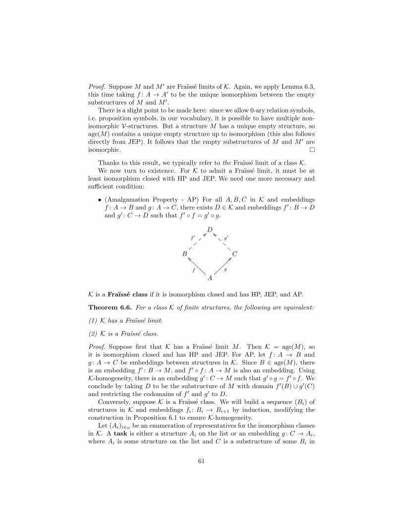
Proof. Suppose M and M ′ are Fraısse limits of K. Again, we apply Lemma 6.3,this time taking f : A → A′ to be the unique isomorphism between the emptysubstructures of M and M ′.
There is a slight point to be made here: since we allow 0-ary relation symbols,i.e. proposition symbols, in our vocabulary, it is possible to have multiple non-isomorphic V-structures. But a structure M has a unique empty structure, soage(M) contains a unique empty structure up to isomorphism (this also followsdirectly from JEP). It follows that the empty substructures of M and M ′ areisomorphic.
Thanks to this result, we typically refer to the Fraısse limit of a class K.We now turn to existence. For K to admit a Fraısse limit, it must be at
least isomorphism closed with HP and JEP. We need one more necessary andsufficient condition:
• (Amalgamation Property - AP) For all A,B,C in K and embeddingsf : A→ B and g : A→ C, there exists D ∈ K and embeddings f ′ : B → Dand g′ : C → D such that f ′ ◦ f = g′ ◦ g.
D
B
f ′>>
C
g′``
A
f
``
g
>>
K is a Fraısse class if it is isomorphism closed and has HP, JEP, and AP.
Theorem 6.6. For a class K of finite structures, the following are equivalent:
(1) K has a Fraısse limit.
(2) K is a Fraısse class.
Proof. Suppose first that K has a Fraısse limit M . Then K = age(M), soit is isomorphism closed and has HP and JEP. For AP, let f : A → B andg : A → C be embeddings between structures in K. Since B ∈ age(M), thereis an embedding f ′ : B → M , and f ′ ◦ f : A→ M is also an embedding. UsingK-homogeneity, there is an embedding g′ : C →M such that g′ ◦ g = f ′ ◦ f . Weconclude by taking D to be the substructure of M with domain f ′(B) ∪ g′(C)and restricting the codomains of f ′ and g′ to D.
Conversely, suppose K is a Fraısse class. We will build a sequence (Bi) ofstructures in K and embeddings fi : Bi → Bi+1 by induction, modifying theconstruction in Proposition 6.1 to ensure K-homogeneity.
Let (Ai)i∈ω be an enumeration of representatives for the isomorphism classesin K. A task is either a structure Ai on the list or an embedding g : C → Ai,where Ai is some structure on the list and C is a substructure of some Bi in
61

our inductive construction. We will list the tasks by pairs in ω × ω. To start,define task (i, 0) to be the structure Ai. We will define tasks (i, j) for j > 0during stage i of the construction. Fix a bijection17 t : ω → ω × ω such thatt(0) = (0, 0) and t(n) = (m,m′) with m < n for all n > 0 (this ensures that taskt(n) has already been defined before stage n). We will accomplish task t(n) atstage n of the construction.
At stage 0, let B0 = A0. This completes task t(0) = (0, 0), by ensuring thatA0 embeds in B0. See the general case below for how to define the tasks (0, j)for j > 0.
At stage n, we are given Bn−1 and a task t(n). If this task is a structureAi, use JEP to embed Bn−1 and Ai into a structure Bn in K. On the otherhand, if the task is an embedding g : C → Ai, where C is a substructure of someBk with k < n, let f : C → Bn−1 be the embedding obtained by restrictingthe embedding Bk → Bn−1 to C. Then use AP to embed Bn−1 and C into astructure Bn in K in a way that makes the square over C commute.
Bk // . . . // Bn
C
OO
// Ai
OO
We finish stage n by defining the tasks (n, j) for j > 0. Enumerate theembeddings gj : C → Ai, where C is a substructure of Bn and Ai is on our listof isomorphism representatives. There are countably many such embeddings,since Bn has finitely many finite substructures C, there are countably many ofthe Ai, and for fixed C and Ai, there are finitely many embeddings C → Ai.Define task (n, j) to be the embedding gj−1.
After defining the entire sequence (Bn)n∈ω, we have also completed everytask. Let M = lim−→Bn. Then M is countable, since it is a directed colimit offinite structuers, and age(M) = K exactly as in Proposition 6.1. It remains tocheck K-homogeneity.
So suppose f : C → M and g : C → A are embeddings, with A,C ∈ K.Then the image of C in M is contained in the image of some Bn, so f = σn ◦f ′,for some f ′ : C → Bn, where σn : Bn → M is the canonical embedding. Aftercomposing with isomorphisms, we can safely assume that C is a substructureof Bn and A is Ai for some i. So g : C → A was added as a task (n, j) = t(m)for some j, and there is an embedding A → Bm making the square commute.Composing with the canonical embedding σm : Bm →M finishes the proof.
Example 6.7. Here are some examples of Fraısse classes and their Fraısse limit.
• The class of finite graphs. The Fraısse limit is called the random graph(or the Rado graph), which we will discuss further below.
17The usual “diagonals” bijection, which enumerates ω × ω as (0, 0), (0, 1), (1, 0), (0, 2),(1, 1), (2, 0),. . . works.
62

• The class of finite triangle-free graphs. The Fraısse limit is called theHenson graph.
• The class of finite linear orders. The Fraısse limit is the countable denselinear order without endpoints (Q, <).
• The class of finite equivalence relations. The Fraısse limit is the equiva-lence relation with countably infinitely many countably infinite classes.
Example 6.8. The simplest isomorphism-closed class of finite structures withHP and JEP but not AP is the class of acyclic graphs, also known as forests18.Let A consist of two vertices x and y, not connected by an edge. Let B be Atogether with a new vertex connecting x and y by a path of length 2. And letC be A together with two new vertices conncting x and y by a path of length3. Then B and C cannot be amalgamated over A.
When the vocabulary is finite, for any finite structure A, enumerated (ai)ni=1,
there is a quantifier-free formula θA(x1, . . . , xn) such that B |= θA(b1, . . . , bn) ifand only if the map ai 7→ bi is an embedding A→ B. This formula is essentiallyjust the conjunction of all atomic formulas true in A (see Proposition 4.10).
Now if K is a Fraısse class, we can axiomatize the theory of Fraısse limits ofK as follows:
• ∀ axioms for K: For every finite structure A not in K, let χA be
∀x1 . . . ∀xn¬θA(x1, . . . , xn).
• ∀∃ extension axioms: For every finite structure B in K enumerated (bi)ni=1
and every substructure A ⊆ B which is an initial segment in the enumer-ation, (bi)
mi=1 for 0 ≤ m ≤ n, let ϕA,B be
∀x1 . . . ∀xm(θA(x1, . . . , xm)→ ∃xm+1 . . . ∃xn θB(x1, . . . , xn)).
We call TK, the set of all axioms of the above forms, the generic theoryof K. If M |= TK and M is countable, then M is a Fraısse limit of K.
• Since M |= χA for all A /∈ K, no structure not in K embeds in M , soage(M) ⊆ K. The converse follows from K-homogeneity, since for anystructure B in K, the empty substructure of B is isomorphic to the emptysubstructure of M (K contains a unique empty structure, by HP and JEP),so B embeds in M over the empty structure.
• For K-homogeneity, suppose f : A → M and g : A → B are embeddingswith A and B in K. We may assume A is a substructure of B. EnumerateB as (bi)
ni=1, ensuring that A is the initial segment (bi)
mi=1. Then M |=
θA(f(b1), . . . , f(bm)), and M |= ϕA,B , so there exists cm+1, . . . , cn suchthat M |= θB(f(b1), . . . , f(bm), cm+1, . . . , cn). Extend f to a map B →Mby bi 7→ ci for all m < i ≤ n.
18A tree is a connected acyclic graph, and a forest is a disjoint union of trees
63

When K contains arbitrarily large finite structures, it follows that TK isℵ0-categorical, and hence complete by Vaught’s test.
It is often possible to give a simpler axiomatization of TK than the oneTuesday 10/30described above. One simplification which is always possible is to assume in theextension axiom ϕA,B that |B| = |A|+ 1. We call such an axiom a one-pointextension axiom. Indeed, if M satisfies all one-point extension axioms, thenit is easy to show that it is K-homogeneous by induction on |B|− |A|, extendingan embedding of A into M to B one point at a time.
Here are some further examples of simplifications of TK.
Example 6.9. Let Klo be the class of finite linear orders. The universal partof TKlo
can be axiomatized by the theory of linear orders:
∀x∀y∀z ((x < y ∧ y < z)→ x < z)
∀x∀y (x < y ∨ y < x ∨ x = y)
∀x¬(x < x)
Indeed, if M satisfies the three sentences above, then already age(M) ⊆ Klo.The ∀∃ part of TKlo
can be reduced to the following axioms:
∀x∃y x < y
∀x∃y y < x
∀x∀y(x < y → ∃z (x < z ∧ z < y))
Indeed, if M satisfies all six of the sentences above, then it satisfies all of theone-point extension axioms. For any finite subset A ⊆ M and any embeddingA → B where |B| = |A| + 1, the new element in b is either greater than everypoint in A, less than every point in A, or between two points of A, and one ofthe three ∀∃-sentences above handles each of those cases.
Of course, this verifies that the Fraısse limit of Klo is the countable denselinear order without endpoints.
Example 6.10. Let G be the class of finite graphs. The universal part of TGcan be axiomatized by the theory of graphs:
∀x¬(xEx)
∀x∀y (xEy → yEx)
Indeed, if M satisfies the two sentences above, then already age(M) ⊆ G.The ∀∃ part of TG can be reduced to the following schema, one sentence
ϕm,n for every pair m,n ∈ ω:
∀x1 . . . ∀xm∀y1 . . . ∀yn
∧i,j
xi 6= yj
→ ∃z ∧1≤i≤m
zExi ∧∧
1≤j≤n
¬zEyj
This is simpler than the general one-point extension axiom ϕA,B since we don’thave to describe the graph structure on A = {x1, . . . , xm, y1, . . . , yn}, we justneed to know which elements of A the new element z connects to.
64

In the case of linear orders, we have a concrete representative of the Fraısselimit, namely (Q, <). The Fraısse limit of the class of finite graphs a bit morecomplicated. However, there are several pleasant presentations of this structure.Here are two of them:
• Consider the relation E on ω, defined by mEn if and only if n < m andthe binary expansion of m has a 1 in the nth position (the 2n place), orm < n and the binary expansion of n has a 1 in the mth position (the 2m
place). Then (ω,E) is a Fraısse limit of G.
Indeed, E is a symmetric and irreflexive binary relation on ω, and givenany distinct numbers x1, . . . , xm, y1, . . . , yn ∈ ω, we can find a naturalnumber which is greater than all of these numbers and whose binary ex-pansion ensures it is related to x1, . . . , xm and not related to y1, . . . , yn.
• Build a graph with domain ω at random as follows: For every pair {m,n}with m 6= n, flip a coin and put an edge between n and m if it comes upheads. That is, mEn and nEm holds with probability 1/2, independentlyfor all pairs {m,n}. This is called the Erdos–Renyi coin-flipping process.Then, with probability 1, (ω,E) is a Fraısse limit of G. This is why theFraısse limit of G is called the random graph.
We can check this with a simple probabilistic argument. Consider afixed one-point extension axiom ϕm,n. Suppose we have distinct elementsx1, . . . , xm, y1, . . . , yn from ω. For any z not among these elements, theprobability that z is a witness for the extension axiom (i.e. z is connectedto the xi and not connected to the yj) is exactly 2−(m+n). And crucially,the probabilities that z and z′ are witnesses are independent. Since thereare infinitely many z not among the xi and yj , we have infinitely many in-dependent chances to find a witness, each with positive probability. By theBorel-Cantelli Lemma, we find infinitely many witnesses in ω with proba-bility 1. Now there are countably many sequences of xi and yj , there arecountably many extension axioms, and the intersection of countably manyprobability 1 events has probability 1. So (ω,E) |= TG with probability 1.
A variant of the probabilistic argument above gives a remarkable fact: thefirst-order zero-one law for the class of finite graphs.
Let K be an isomorphism-closed class of finite structures which contains atleast one structure of size n for each n ∈ ω. Write K[n] for the set of structuresin K with domain [n] = {1, . . . , n}. We write
Pn(ϕ) =|{A ∈ K[n] | A |= ϕ}|
|K[n]|
for the probability that a structure A in K[n], selected uniformly at random,satisfies ϕ. The asymptotic probability of ϕ is limn→∞ Pn(ϕ), if this limitexists.
The almost-sure theory of K is the set of all sentences with asymptoticprobability 1. This is the set of first-order properties of structures in K thathold of almost all large finite structures in K.
65

Lemma 6.11. The almost-sure theory Tas of K is consistent and closed underentailment.
Proof. We first show that Tas is closed under entailment. Suppose Tas |= θ.
Then there are finitely many sentences ψ1, . . . , ψk ∈ Tas such that∧ki=1 ψi |= θ.
Since each ψi has asymptotic probability 1, for any ε > 0, there is some N suchthat for all n > N and all 1 ≤ i ≤ k,
Pn(ψi) ≥ 1− ε/k.
Since Pn(¬ψi) ≤ ε/k, we have Pn(¬∧ki=1 ψi) ≤ ε. And since
∧ki=1 ψi |= θ, it
follows that
Pn(θ) ≥ Pn
(k∧i=1
ψi
)≥ 1− ε.
So limn→∞ Pn(θ) = 1, and θ ∈ Tas.It follows that Tas is consistent. If not, then Tas |= ⊥, so ⊥ ∈ Tas, and
limn→∞ Pn(⊥) = 1, but Pn(⊥) = 0 for all n, which is a contradiction.
We say that K has a first-order zero-one law if for every sentence ϕ,
limn→∞
Pn(ϕ) = 0 or 1.
Equivalently, K has a first-order zero-one law if and only if its almost-sure theoryis complete.
Theorem 6.12. Let G be the class of all finite graphs. Then G has a first-orderThursday 11/1zero-one law, and its almost-sure theory is equivalent to TG, the theory of therandom graph.
Proof. The proof has two components: a logical argument and a probabilisticargument. We deal with the logical argument first.
Claim: It suffices to show that every one-point extension axiom ϕm,n hasasymptotic probability 1.
Let Tas be the almost-sure theory of G. Since the axioms of the theory ofgraphs hold of all structures in G, these sentences have asymptotic probability 1.Assuming also that every one-point extension axiom has asymptotic probability1, we have TG ⊆ Tas. By Lemma 6.11, every consequence of TG is in Tas.
But since TG is complete and Tas is consistent, Tas must be equal to the setof consequences of TG . So Tas is complete, and G has a first-order zero-one law.
Having established the claim, we fix a one-point extension axiom ϕm,n, andlet m + n = k. Observe that the uniform probability measure PN on G[N ]
agrees with the Erdos–Renyi coin-flipping process: for any {i, j} ⊆ [N ] withi 6= j, exactly half of the graphs in G[N ] have iEj, and these probabilities areindependent between pairs.
Now fix some distinct x1, . . . , xm, y1, . . . , yn ∈ [N ]. The probability thatsome z is a witness to the extension axiom ϕm,n for these xi and yj is 2−(m+n).
66

Define δ = 2−(m+n) > 0. There are N − k possible witnesses z, and each is awitness with probability δ, independently. So the probability that there is nowitness to the extension axiom over the xi and yj is (1− δ)N−k. It follows that
PN (¬ϕm,n) ≤ Nk(1− δ)N−k,
since Nk is an upper bound for the number of choices of the xi and yj .Now when we compute limN→∞ PN (¬ϕm,n), k is fixed and N grows, so the
polynomial Nk is dominated by the exponential decay (1−δ)N−k (since 1−δ <1), and limN→∞ PN (¬ϕm,n) = 0. Hence, ϕm,n has asymptotic probability 1.
Example 6.13. To see the necessity of considering properties expressible byfirst-order sentences, note that the following limit does not exist:
limn→∞
|{A ∈ K[n] | |A| is even}||K[n]|
.
Indeed, the property “|A| is even” is not expressible by a first-order sentencerelative to the theory of graphs.
We have also seen that the property “A is connected” is not expressible bya first-order sentence relative to the theory of graphs. However, the randomgraph is connected with diameter 2, since it satisfies ∀x∀y∃z (xEz ∧ zEy). Itfollows that this sentence is in the almost-sure theory of G: almost all largefinite graphs have diameter 2, so almost all large finite graphs are connected.
Exercise 24. Let K be the class of all finite V-structures, for any single-sortedfinite relational vocabulary V.
(a) Show that K is a Fraısse class, and axiomatize its generic theory TK.
(b) Show that K has a first-order zero-one law, and its almost-sure theory is TK(the argument will be very similar to the argument for the random graph).
When there are function symbols in the language, we typically do not havea first-order zero-one law, as the following exercise demonstrates.
Exercise 25. Let V be the vocabulary with a single unary function symbol f .Let K be the class of all finite V structures. Let ϕ be the sentence ∀x (f(x) 6= x).Show that
limn→∞
Pn(ϕ) =1
e.
Example 6.14. Let G4 be the class of all finite triangle-free graphs. Erdos,Kleitman, and Rothschild showed that almost all triangle-free graphs are bipar-tite, i.e.
limn→∞
|{A ∈ (G4)[n] | A is bipartite}||(G4)[n]|
= 1.
Kolaitis, Promel, and Rothschild refined this result, showing that G4 has afirst-order zero-one law, and its almost-sure theory is equal to the generic theory
67

of bipartite graphs. To be more precise, the class of all finite bipartite graphsin the vocabulary of graphs is not a Fraısse class (it fails amalgamation, sincepaths of lengths 2 and 3 cannot be amalgamated over their endpoints). Butif we view bipartite graphs in the vocabulary Vbi = (E,L,R), where L and Rare unary relations naming the bipartition, then the class Gbi of finite bipartitegraphs is a Fraısse class, with a generic theory TGbi . And the theorem is that thealmost-sure theory of G4 is equal to the subtheory of TGbi consisting of thosesentences which do not mention L and R.
In particular, the almost-sure theory of G4 is not equal to the generic theoryTG4 , since the Fraısse limit of G4 contains odd-length cycles (for example, thepentagon), which cannot be embedded in any bipartite graph. This raises aninteresting question (which is a major open problem at the border of model the-ory and combinatorics): We say that a theory has the finite model propertyif every sentence in the theory has a finite model. The theory of the randomgraph, TG , has the finite model property (in fact, almost all finite graphs aremodels, by the zero-one law). Does TG4 have the finite model property?
It is even an open question whether there exists a finite triangle-free graphsatisfying the one-point extension axioms over subsets of size at most 4.
6.2 Quantifier elimination
A theory T has quantifier elimination if every formula is T -equivalent to aquantifier-free formula.
This notion is extremely important in “applied” model theory: If we want tounderstand a given first-order theory, the first step is to understand the defin-able sets, i.e. the formulas up to T -equivalence. And in the best-case scenario,when T has quantifier elimination, we find that every definable set is a Booleancombination of sets defined by atomic formulas, which are hopefully easy tounderstand.
For M |= T and a ∈Mx, define
qftp(a) = {ϕ(x) | ϕ is quantifier-free and M |= ϕ(a)}.
Note that qftp(a) ⊆ tp(a). Intuitively, qftp(a) describes the isomorphism-type of the substructure 〈a〉 of M generated by a.
Proposition 6.15. Let a ∈ Mx and a′ ∈ (M ′)x, where M and M ′ are modelsof T . Then qftp(a) = qftp(a′) if and only if 〈a〉 ∼= 〈a′〉 by an isomorphismmapping a to a′.
Proof. Let A = 〈a〉 and A′ = 〈a′〉. Suppose f : A→ A′ is an isomorphism withf(a) = a′. Let ϕ(x) be a quantifier-free formula. Then ϕ(x) is both universaland existential, so it is preserved and reflected by embeddings (in particular,the inclusions A→M and A′ →M ′ and the isomorphism f : A→ A′). Then:
M |= ϕ(a) ⇐⇒ A |= ϕ(a)
⇐⇒ A′ |= ϕ(f(a))
⇐⇒ M ′ |= ϕ(a′).
68

So qftp(a) = qftp(a′).Conversely, suppose qftp(a) = qftp(a′). Recall (Exercise 1), that b ∈ A = 〈a〉
if and only if there is some term t(x) such that b = tM (a), and similarly forA′ = 〈a′〉 (of course, the term t need not be unique).
Define a map f : A→ A′ by f(tM (a)) = tM′(a′). This is well-defined, since
if tM (a) = (t′)M (a), then the formula t(x) = t′(x) is in qftp(a) = qftp(a′), sotM′(a′) = (t′)M
′(a′).
1. f is injective: If tM (a) 6= (t′)M (a), then t(x) 6= t′(x) is in qftp(a′), sotM′(a′) 6= (t′)M
′(a′).
2. f is surjective: For any b ∈ A′, b = tM′(a′) for some term t(x), and
b = f(tM (a)).
3. f maps a to a′. Any element ai from the tuple a is equal to tM (a) wheret(x) is the variable xi. Then f(ai) = tM
′(a′) = a′i.
4. f respects functions symbols. For any function symbol g and termst1(x), . . . , tn(x) of the appropriate types, let t(x) be the composite termg(t1, . . . , tn). Then we have
f(gM (tM1 (a), . . . , tMn (a))) = f(tM (a))
= tM′(a′)
= gM′(tM
′
1 (a′), . . . , tM′
n (a′))
= gM′(f(tM1 (a)), . . . , f(tMn (a))).
5. f preserves and reflects relation symbols. For any relation symbol R andterms t1(x), . . . , tn(x) of the appropriate types, let ϕ(x) be the quantifier-free formula R(t1, . . . , tn). Then we have
(tM1 (a), . . . , tMn (a)) ∈ RM ⇐⇒ ϕ(x) ∈ qftp(a)
⇐⇒ ϕ(x) ∈ qftp(a′)
⇐⇒ (tM′
1 (a′), . . . , tM′
n (a′)) ∈ RM′
⇐⇒ (f(tM1 (a)), . . . , f(tMn (a))) ∈ RM .
Our first test for quantifier elimination is simple: if complete types are de-termined by quantifier-free types, then T has quantifier-elimination.
Proposition 6.16. Suppose that for all contexts x and all complete types p andq in Sx(T ), if p and q contain the same quantifier-free formulas, then p = q.Then T has quantifier elimination.
Proof. Let ϕ(x) be any formula, and consider complete types p and q suchthat ϕ(x) ∈ p and ϕ(x) /∈ q. Then p 6= q, so p and q do not contain thesame quantifier-free formulas. Since the quantifier-free formulas are closed undernegation, we may assume there is some quantifier-free formula ψ(x) such thatψ(x) ∈ p and ψ(x) /∈ q. By Corollary 5.8, ϕ(x) is T -equivalent to a quantifier-free formula.
69

As an application of this test, we can show easily that theories of Fraısselimits eliminate quantifiers.
Corollary 6.17. Let V be a single-sorted finite relational vocabulary, and letK be a Fraısse class of V-structures. The generic theory TK has quantifierelimination.
Proof. We apply Proposition 6.16. Suppose p and q are complete types inSx(TK) which contain the same quantifier-free formulas. Let M |= TK be acountable model and a, a′ ∈ Mx such that M |= p(a) and M |= q(a′). (How?Find a realization a of p in M1 |= TK, and then find a realization a′ of q in anelementary extension M1 �M2 by Proposition 5.3, and finally take a countableelementary substructure M �M2 containing a and a′ by Lowenheim–Skolem.)
Now M is a Fraısse limit of K. And since p and q contain the same quantifier-free formulas, 〈a〉 and 〈a′〉 are isomorphic by an isomorphism mapping a toa′. By strong K-homogeneity, this isomorphism extends to an automorphismσ : M → M such that σ(a) = a′. But then tp(a) = tp(a′), so p = q. ByProposition 6.16, TK has quantifier elimination.
We will now develop a slightly more refined test for quantifier-elimination.Tuesday 11/6First, we reduce the problem on the syntactic side, then we prove a semanticequivalence.
A formula ϕ(x) is primitive existential if it has the form ∃y ψ(x, y), wherey is a single variable and ψ(x, y) is a conjunction of atomic and negated atomicformulas.
Lemma 6.18. Suppose that every primitive existential formula is T -equivalentto a quantifier-free formula. Then T has quantifier elimination.
Proof. We prove by induction that every formula is T -equivalent to a quantifier-free formula. This is clear for atomic formulas, and the induction steps forBoolean combinations are trivial. So it suffices to consider the case of a formula∃y ψ(x, y). By the inductive hypothesis, ψ(x, y) is T -equivalent to a quantifier-free formula ϕ(x, y), which is logically equivalent to a formula in disjunctivenormal form (Exercise 19),
n∨i=1
ϕi(x, y),
where each ϕi is a conjunction of atomic and negated atomic formulas. So∃y ψ(x, y) is T -equivalent to
∃yn∨i=1
ϕi(x, y),
which is logically equivalent to
n∨i=1
∃y ϕi(x, y).
70

Now each formula ∃y ϕi(x, y) is primitive existential, so by assumption it isT -equivalent to a quantifier-free formula χi(x, y), and our original formula isT -equivalent to
∨ni=1 χi(x, y).
Let M and M ′ be V-structures, and suppose A ⊆M . A map f : A→M ′ ispartial elementary if for all formulas ϕ(x) and all a ∈ Ax, M |= ϕ(a) if andonly if M ′ |= ϕ(f(a)).
Theorem 6.19. The following are equivalent:
(1) T has quantifier elimination.
(2) For any models M |= T and M ′ |= T , if A is a substructure of M andf : A→M ′ is an embedding, then f is partial elementary.
(3) For any models M |= T and M ′ |= T , if A is a finitely generated substructureof M , f : A → M ′ is an embedding, and ϕ(x) is a primitive existentialformula, then for all a ∈ Ax, if M |= ϕ(a), then M ′ |= ϕ(f(a)).
Proof. (1)⇒(2): Suppose T has quantifier elimination and f : A → M ′ is anembedding, where A is a substructure of M |= T , and M ′ |= T . Let ϕ(x) bea formula and a ∈ Ax. Then ϕ(x) is T -equivalent to a quantifier-free formulaψ(x). Since ψ(x) is both universal and existential, it is preserved and reflectedby embeddings. So
M |= ϕ(a) ⇐⇒ M |= ψ(a)
⇐⇒ A |= ψ(a)
⇐⇒ M ′ |= ψ(f(a))
⇐⇒ M ′ |= ϕ(f(a)).
(2)⇒(3): Trivial from the definition of partial elementary map.(3)⇒(1): By Lemma 6.18, it suffices to show that every primitive existential
formula is equivalent to a quantifier-free formula. We apply the separationlemma for formulas, Corollary 5.8. So let ϕ(x) be a primitive existential formula,and let p(x) and q(x) be complete types such that ϕ(x) ∈ p(x) and ϕ(x) /∈ q(x).Suppose for contradiction that no quantifier-free formula separates p from q, i.e.(since quantifier-free formulas are closed under negation) that p and q containthe same quantifier-free formulas.
Let a ∈ Mx and a′ ∈ (M ′)x with M,M ′ |= T , M |= p(a), and M ′ |= q(a′).LetA = 〈a〉 andA′ = 〈a′〉. In particular, A is a finitely generated substructure ofM . Since p and q contain the same quantifier-free formulas, qftp(a) = qftp(a′),so A ∼= A′ by an isomorphism mapping a to a′. We may view this isomorphismas an embedding f : A → M ′. But then ϕ(x) ∈ p(x) implies M |= ϕ(a), so byassumption M ′ |= ϕ(a′), and ϕ(x) ∈ q(x), contradiction.
As an application, we prove that the theory of algebraically closed fields hasquantifier elimination.
Theorem 6.20. ACF has quantifier elimination.
71

Proof. We use the test in Theorem 6.19. So suppose K and K ′ are algebraicallyclosed fields, A ⊆ K is a finitely generated substructure, and f : A → K ′ is anembedding. Let ∃y ϕ(x, y) be a primitive existential formula, and let a ∈ Axsuch that K |= ∃y ϕ(a, y).
Let B = f(A), so f can be viewed as an isomorphism A ∼= B. Now A and Bare subrings of K and K ′, respectively. Let A1 and B1 be the subfields of K andK ′ generated by A and B, respectively. So A1
∼= Frac(A) and B1∼= Frac(B),
and f extends to an isomorphism f1 : A1∼= B1.
Let A2 and B2 be the relative algebraic closures of A1 and B1 inside Kand K ′, respectively. Since K and K ′ are algebraically closed, A2 and B2
are isomorphic to the algebraic closures of A1 and B1, and f1 extends to anisomorphism F2 : A2
∼= B2.Now let b ∈ K such that K |= ϕ(a, b). Let A3 = A2(b), the subfield of K
generated by A2 and b, and let K ′′ be a proper elementary extension of K ′ (thisexists because K ′ is infinite, i.e. not boring). We claim that we can find anembedding g : A2(b)→ K ′′.
Case 1: b ∈ A2. Then A2(b) = A2, and we can take g = f2 (composed withthe inclusions B2 ⊆ K ′ � K ′′).
Case 2: b /∈ A2. Then since A2 is relatively algebraically closed in K, thefield A2(b) is a transcendental extension of A2, isomorphic to A2(x). Since K ′′
is a proper extension of B2, and B2 is algebraically closed, any b′ ∈ K ′′ \ B2 istranscendental over B2. So B2(b′) is isomorphic to B2(x), and f2 extends to anisomorphism f3 : A2(b) ∼= B2(b′), which we view as an embedding A2(b)→ K ′′.
Note that we only needed the elementary extension K ′′ to handle the casewhen K ′ doesn’t already contain an element transcendental over B2, i.e. whenK ′ = B2.
K K ′′
A2(b)
f3
<<
K ′
�
A2f2 // B2
A1f1 // B1
Af // B
To finish, observe that since K |= ϕ(a, b), and ϕ(x, y) is quantifier-free, wehave A2(b) |= ϕ(a, b), so K ′′ |= ϕ(f3(a), f3(b)), so K ′′ |= ∃y ϕ(f(a), y), and sinceK ′ � K ′′, also K ′ |= ∃y ϕ(f(a), y), as desired.
Let’s think about what this theorem means in context. The vocabulary of
72

rings has no relation symbols, so every atomic formula has the form t(x) = t′(x),where t and t′ are terms in context x. Modulo the theory of rings, this formulais equivalent to t(x)−t′(x) = 0, and each term can be rewritten as a polynomial,so every atomic formula is equivalent to one of the form p(x) = 0, where p is apolynomial. The definable set {x ∈ Kn | p(x) = 0} is a closed set in the Zariskitopology on Kn. On the other hand, the negated atomic formula p(x) 6= 0defines a Zariski open set.
Now a quantifier-free formula ϕ(x) defines a Boolean combination of Zariskiclosed sets. Such a set is called a constructible set19.
As we have noted before, the operation of adding an existential quantifier to aformula corresponds to the coordinate projection of definable sets. For example,the projection of the set {(x, y) ∈ K2 | xy = 1} onto the first coordinate is theset {x ∈ K | x 6= 0}. This corresponds to the fact that the formula ∃y (xy = 1)is ACF-equivalent to the quantifier-free formula x 6= 0.
Keeping this in mind, we find that quantifier elimination for ACF is equiv-alent to (a form of) Chevalley’s theorem on constructible sets. Of course, thereare fancier scheme-theoretic versions of this theorem in algebraic geometry.
Corollary 6.21 (Chevalley’s theorem). A coordinate projection of a Zariskiconstructible set is Zariski constructible.
Quantifier elimination can also be a tool for proving completeness.
Proposition 6.22. (1) If T is complete, then all models of T have isomorphicminimal substructures. That is, for any M,M ′ |= T , 〈∅〉M ∼= 〈∅〉M ′ .
(2) The converse is true if T has quantifier elimination.
(3) If V has no 0-ary function symbols (constant symbols) or 0-ary relation sym-bols (proposition symbols), then quantifier elimination implies completeness.
Proof. For (1), suppose T is complete. Then the quantifier-free type of theempty tuple in M |= T is the set of all quantifier-free sentences true in M . SinceT is complete, every quantifier-free sentence true in M is entailed by T . So ifM,M ′ |= T , qftpM (∅) = qftpM ′(∅). Then 〈∅〉M ∼= 〈∅〉M ′ by Proposition 6.15.
For (2), suppose that T has quantifier elimination and all models of T haveisomorphic minimal substructures. Suppose for contradiction that T is notcomplete. Then there is a sentence ϕ and models M |= T ∪ {ϕ} and M ′ |=T ∪ {¬ϕ}. But the isomorphism 〈∅〉M → 〈∅〉M ′ is a partial elementary map byTheorem 6.19, so M |= ϕ if and only if M ′ |= ϕ, contradiction.
For (3), note that if V has no constant symbols, then 〈∅〉M is empty for allV-structures M . And if V has no proposition symbols, then there is a uniqueempty V-structure up to isomorphism. It follows that for any M,M ′ |= T ,〈∅〉M ∼= 〈∅〉M ′ .
19Sometimes a constructible set is defined to be a finite union of locally closed sets, i.e. setswhich are open in their closure. This is equivalent: a locally closed set is the intersection ofan open set and a closed set, and any Boolean combination of closed sets can be written as afinite union of locally closed sets, thanks to the disjunctive normal form
73

Another way of proving (3) is to note that if T has quantifier-elimination,then every sentence is T -equivalent to a quantifier-free sentence. But if there areno constant symbols or proposition symbols, the only quantifier-free sentencesare > and ⊥.
This gives us a new proof that for fixed p, either prime or 0, the theory ACFpis complete. Indeed, since ACF ⊆ ACFp, ACFp has quantifier elimination. Andfor any M,M ′ |= ACFp, 〈∅〉M ∼= 〈∅〉M ′ ∼= Fp.
If a theory T has a reasonable (meaning computable) axiomatization, thenas soon as we know T is complete, we have an algorithm for deciding whichsentences are entailed by T . For any sentence ϕ, start searching for a proofT ` ϕ, and simultaneously start searching for a proof T ` ¬ϕ. Since T iscomplete, one of these searches eventually terminates.
But the algorithm described above is hopelessly inefficient. In many situa-tions, a more efficient algorithm can be found via effective quantifier elimination,i.e. an algorithm for finding a quantifier-free formula which is T -equivalent toa given formula. Applying this algorithm to an arbitrary sentence ϕ producesa quantifier-free sentence ψ which is T -equivalent to it. But a quantifier-freesentence ψ is just a Boolean combination of atomic statements about 〈∅〉, thetruth value of which can be easily checked.
The proof we gave above that ACF has quantifier elimination was entirelyineffective. But an effective quantifier elimination algorithm exists for ACF; inthis case, a quantifier-free sentences comes down to an explicit list of the char-acteristics p in which the sentence is true. And effective quantifier eliminationalgorithms also exist for other interesting theories, like Th(R; 0, 1,+,−, ·,≤),the theory of real closed ordered fields (this is know as Tarski’s Theorem).
Exercise 26. Let s : ω → ω be the successor function n 7→ n + 1. Show thatTh(ω; s) does not have quantifier elimination, but Th(ω; s, 0) does (where 0 isa constant symbol naming the element 0).
Exercise 27. Let K be a field, and let T be the theory of infinite vectorspaces over K in the single-sorted vocabulary of Example 1.2. Show that T hasquantifier elimination.
Exercise 28. Let T be the theory of infinite-dimensional vector spaces overalgebraically closed fields of characteristic 0 in the two-sorted vocabulary ofExample 1.1. That is, T consists of the vector space axioms, the axioms ofACF0 in the field sort k, and axioms asserting that the vector space v is notn-dimensional for any n (if it is not clear to you how to axiomatize this theory,then you can consider it part of the exercise). Show that T does not havequantifier elimination.
6.3 Model completeness and model companions
One advantage of showing that T has quantifier elimination is that the notions ofThursday 11/8elementary embedding and elementary substructure become much simpler. If T
74

has quantifier elimination, then every embedding between models of T is an ele-mentary embedding (every formula is T -equivalent to a quantifier-free formula,and quantifier-free formulas are preserved and reflected by embeddings).
Some theories have this nice property, without having quantifier eliminationin full. A theory T is model complete if every embedding between models ofT is an elementary embedding.
Part (a) of the following exercise explains the name “model complete”. Part(b) shows that quantifier elimination could also be called “substructure com-pleteness”.
Exercise 29. (a) Show that T is model complete if and only if for any modelM |= T , T ∪Diag(M) is a complete V(M)-theory.
(b) Show that T has quantifier elimination if and only if for any model M |= T ,and any substructure A ⊆M , T ∪Diag(A) is a complete V(A)-theory.
Proposition 6.23. Every model complete theory T has a ∀∃ axiomatization,i.e. T is equivalent to a ∀∃-theory.
Proof. By Theorem 5.15, it suffices to show that T is preserved by directedcolimits. So suppose (Mi)i∈I is a directed system of V-structures, such thatMi |= T for all i ∈ I, and let M = lim−→Mi. Since T is model complete, this isa directed colimit along elementary embeddings, so by Proposition 5.13, eachmap σi : Mi →M is an elementary embedding. In particular, M |= T .
Example 6.24. In 1996, Wilkie showed that Th(R; 0, 1,+,−, ·, ex), where ex
is viewed as a unary function symbol, is model complete. It follows that thistheory has a ∀∃ axiomatization, but we don’t know what it is. In fact, givingan explicit axiomatization of this theory would almost certainly require provingthe real Schanuel’s conjecture: If x1, . . . , xn are real numbers such thatQ(x1, . . . , xn, e
x1 , . . . , exn) has transcendence degree less than n over Q, thenx1, . . . , xn are linearly dependent over Q.
Suppose M ⊆ N are V-structures. We say that M is existentially closedin N if for any ∃-formula ϕ(x) and any a ∈Mx, if N |= ϕ(a), then M |= ϕ(a).We say that a model M |= T is existentially closed (in models of T ) ifwhenever M ⊆ N and N |= T , M is existentially closed in N .
Theorem 6.25. The following are equivalent:
(1) T is model complete.
(2) Every model of T is existentially closed.
(3) Every formula is T -equivalent to a ∀-formula.
(4) Every formula is T -equivalent to an ∃-formula.
75

Proof. (1)⇒(2): If M,N |= T and M ⊆ N , then since T is model complete,M � N , so M is existentially closed in N .
(2)⇒(3): First note that (2) implies that all ∃-formulas are reflected byembeddings between models of T . Indeed, if f : M → N is an embedding,with M,N |= T , then M ∼= f(M) ⊆ N , and f(M) is existentially closed in N .So if N |= ϕ(f(a)), where ϕ(x) is an ∃-formula, then f(M) |= ϕ(f(a)), andM |= ϕ(a).
So by Theorem 5.11, every ∃-formula is T -equivalent to a ∀-formula.We now prove that every formula is T -equivalent to a ∀-formula. By defini-
tion, the class of ∀-formulas contains the atomic formulas and > and ⊥ and isclosed under ∧, ∨, and ∀. So it suffices to show that up to T -equivalence, theclass of ∀-formulas is closed under ¬ and ∃.
For ¬, if ϕ(x) is a ∀-formula, then ¬ϕ(x) is an ∃-formula, which is T -equivalent to a ∀-formula by the observation above. For ∃, if ϕ(x, y) is a ∀-formula, then ∃y ϕ(x, y) is logically equivalent to ¬∀y ¬ϕ(x, y), and we haveshown that the ∀-formulas are closed under ¬ and ∀, up to T -equivalence.
(3)⇔(4): Suppose every formula is T -equivalent to a ∀-formula. Then forany formula ϕ(x), the formula ¬ϕ(x) is T -equivalent to a ∀-formula ψ(x), soϕ(x) is T -equivalent to ¬ϕ(x), which is logically equivalent to an ∃-formula.The converse is similar.
(4)⇒(1): Suppose f : M → N is an embedding, where M,N |= T . Let ϕ(x)be a formula, and let a ∈Mx. By (4) and its equivalent (3), ϕ(x) is T -equivalentto both a universal formula ψ∀(x) (which is reflected by f) and an existentialformula ψ∃(x) (which is preserved by f). So
M |= ϕ(a) =⇒ M |= ψ∃(a)
=⇒ N |= ψ∃(f(a))
=⇒ N |= ϕ(f(a)).
And conversely,
N |= ϕ(f(a)) =⇒ N |= ψ∀(f(a))
=⇒ M |= ψ∀(a)
=⇒ M |= ϕ(a).
This theorem captures the way in which model complete theories come veryclose to having quantifier elimination: every formula is equivalent to both a∀-formula and an ∃-formula, but not necessarily a quantifier-free formula.
Example 6.26. Consider the theory of the real field, T = Th(R; 0, 1,+,−, ·).The relation x ≤ y is T -definable by the formulas
∃z (z · z = y − x) or (x = y) ∨ ∀z (z · z 6= x− y),
but neither of these formulas is T -equivalent to a quantifier-free formula. Indeed,if they were equivalent to ϕ(x, y), then the formula ϕ(x, 0) would define {x ∈R | x ≤ 0}. But ϕ(x, 0) is a Boolean combination of polynomial equations in
76

one variable x. Such a formula can never define an infinite and coinfinite set,since a polynomial in one variable has at most finitely many zeros.
In fact, the theory of the real field is model complete, which we may provelater in these notes, if time permits.
The condition that M is existentially closed can be viewed as an abstractionof the condition that a field is algebraically closed. Indeed, the algebraicallyclosed fields are exactly the existentially closed models of the theory of fields.
As an application, let’s derive Hilbert’s Nullstellensatz as a direct conse-quence of the model completeness of ACF.
Theorem 6.27 (weak Nullstellensatz). Let k be a field, let K be its algebraicclosure, and let I be a proper ideal in the polynomial ring k[x1, . . . , xn]. Thenthere is a tuple (a1, . . . , an) ∈ Kn such that p(a1, . . . , an) = 0 for all p ∈ I.
Proof. Let m be a maximal ideal in k[x1, . . . , xn] extending I. Then the quotientring F = k[x1, . . . , xn]/m is a field, and letting bi = xi + m in F , we havep(b1, . . . , bn) = 0 for all p ∈ I. Let L be the algebraic closure of F . We havea natural embedding k → L, and L is algebraically closed, so we may assumethat k ⊆ K ⊆ L, and by model completeness K is existentially closed in L.
Now I = (p1, . . . , pm) is finitely generated, since k[x1, . . . , xn] is Noetherian(Hilbert’s basis theorem). And L |= ∃x1 . . . ∃xn
∧mi=1 pi(x1, . . . , xn) = 0. This
is an ∃-formula with parameters from k (the coefficients of the pi), so alsoK |= ∃x1 . . . ∃xn
∧mi=1 pi(x1, . . . , xn) = 0, as was to be shown.
We say theories T and T ′ are companions if every model of T embeds in amodel of T ′ and vice versa. We say that T ∗ is a model companion of T if Tand T ∗ are companions and T ∗ is model complete.
Proposition 6.28. If a theory T has a model companion, then it is unique (upto equivalence).
Proof. Suppose T ∗ and T ′ are both model companions of T . Then T ∗ and T ′
are companions (it is easy to see that the companion relation is transitive, infact an equivalence relation on theories).
Let M0 be a model of T ∗. Then M0 embeds in a model N0 |= T ′. And N0
embeds in a model M1 |= T ∗. Continuing in this way, we build a chain:
M0
!!
� // M1
!!
� // . . . M
∼=
N0
==
�// N1
>>
// . . . N
Now letting M = lim−→Mi and N = lim−→Ni, we have M ∼= N . Since T ∗ is modelcomplete, M is a directed colimit along a chain of elementary embeddings, soσ0 : M0 →M is an elementary embedding. Similarly, since T ′ is model complete,N is a directed colimit of models of T ′ along a chain of elementary embeddings,so N |= T ′. So M0 �M ∼= N |= T ′.
77

We have shown that every model of T ∗ is a model of T ′. The symmetricargument shows that T ∗ and T ′ are equivalent.
Example 6.29. The theory of fields and the theory of integral domains areTuesday 11/27companions. Their common model companion is ACF.
Exercise 30. Let K be the class of finite substructures of models of a theoryT , and suppose K is a Fraısse class. Then the generic theory TK is the modelcompanion of T . In particular, the model companion of Th(Z;<) is Th(Q;<).
Exercise 31. For any theory T , let S(T ) be the class of all substructures ofmodels of T , and let T∀ = {ϕ | ϕ is a ∀-sentence, and T |= ϕ} be the set of alluniversal consequences of T . For any theories T and T ′, show that the followingare equivalent:
(1) T and T ′ are companions.
(2) S(T ) = S(T ′).
(3) T∀ = T ′∀.
In the special case that T is a ∀∃-theory, we can characterize the modelcompanion of T in terms of the existentially closed models of T . The mainpoint is the following proposition, which is an abstraction of the fact that everyfield embeds in an algebraically closed field.
Proposition 6.30. Let T be a ∀∃-theory. Then every model of T embeds in anexistentially closed model of T .
Proof. Let M0 be a model of T . For some cardinal κ, let (ϕα)α<κ be an enu-meration of all ∃-formulas with parameters from M0.
We build a directed system (Mα0 )α≤κ of models of T indexed by the directed
set (κ + 1, <), by transfinite induction. Let M00 = M0. For the successor step,
given Mα0 , if there is any N |= T such that Mα
0 ⊆ N and N |= ϕα, then picksome such N and let Mα+1
0 = N . Otherwise, let Mα+10 = Mα
0 .
When β is a nonzero limit ordinal, we have (Mα0 )α<β , such that Mα
0 ⊆Mα′
0
when α ≤ α′, and Mα0 |= T for all α. Let Mβ
0 = lim−→Mα0 . Note that Mβ
0 |= T ,since T is ∀∃ and hence preserved by directed colimits. Finally, let M1 = Mκ
0 .Now we have M0 ⊆ M1, and for any existential formula ϕ with parameters
from M0, if there exists N |= T such that M1 ⊆ N and N |= ϕ, then alreadyM1 |= ϕ. Indeed, ϕ = ϕα for some α, and Mα
0 ⊆ Mα+10 ⊆ M1 ⊆ N , so
Mα+10 |= ϕα, and hence M1 |= ϕα, since ϕα is existential, and hence is preserved
by embeddings.But M1 may not yet be existentially closed, since we’ve only handled exis-
tential formulas with parameters from M0. So we repeat this process, buildinga chain (Mi)i∈ω, such that for any existential formula ϕ with parameters fromMi, if there exists N |= T such that Mi+1 ⊆ N and N |= ϕ, then alreadyMi+1 |= ϕ. Let Mω = lim−→Mi (again, Mω |= T since T is ∀∃).
78

We claim that Mω is existentially closed. Suppose N |= T and Mω ⊆ N , andlet ϕ(a) be an existential formula with a ∈Mx
ω such that N |= ϕ(a). Then thereis some n such that a ∈ Mx
n . We have Mn ⊆ Mω ⊆ N , and by constructionMn+1 |= ϕ(a). So also Mω |= ϕ(a), since ϕ(x) is existential.
Proposition 6.31. Suppose T is a ∀∃ theory, N |= T , and M ⊆ N . If M isexistentially closed in N , then M |= T .
Proof. We show by induction on the construction of ϕ(x) as a ∀∃-formula thatfor all a ∈ Mx, if N |= ϕ(a), then M |= ϕ(a). The conclusion follows, whenapplied to the ∀∃ sentences in T .
The base case, when ϕ(x) is an ∃-formula, is just the fact that M is existen-tially closed in N . And the inductive steps for ∧ and ∨ are easy. So supposethe inductive hypothesis holds for ϕ(x, y), and consider the formula ∀y ϕ(x, y).If a ∈ Mx and N |= ∀y ϕ(a, y), then in particular for all b ∈ My, we haveN |= ϕ(a, b), so by induction M |= ϕ(a, b), and M |= ∀y ϕ(a, y).
Theorem 6.32. Let T be a ∀∃-theory. Then T has a model companion T ∗ ifand only if the class of existentially closed models of T is an elementary class.In this case, T ∗ is the theory of existentially closed models of T .
Proof. Suppose first that the class of existentially closed models of T is ele-mentary, with theory T ∗. We claim that T ∗ is a model companion of T . ByProposition 6.30, every model of T embeds in a model of T ∗, and converselyevery model of T ∗ is itself a model of T . So T ∗ and T are companions. It re-mains to show that T ∗ is model complete. But every model of T ∗ is existentiallyclosed in models of T , so in particular existentially closed in models of T ∗, sowe are done by Theorem 6.25.
Conversely, suppose T has a model companion T ∗. By Proposition 6.23, wemay assume that T ∗ is also a ∀∃-theory. We claim that M |= T ∗ if and only ifM is an existentially closed model of T .
If M is an existentially closed model of T , then because T and T ∗ arecompanions, there are embeddings M ⊆ N ⊆M ′, where N |= T ∗ and M ′ |= T .Then M is existentially closed in N : if ϕ(x) is existential, and N |= ϕ(a), witha ∈ Mx, then M ′ |= ϕ(a), so M |= ϕ(a), since M is existentially closed in M ′.By Proposition 6.31, M |= T ∗, since T ∗ is ∀∃.
In the other direction, if M |= T ∗, we want to show that M is an existentiallyclosed model of T . So suppose M ⊆ N , where N |= T . Since T and T ∗ arecompanions, such anN exists, and for any suchN , there exists a modelM ′ |= T ∗
with M ⊆ N ⊆M ′. Since T ∗ is model complete, M is existentially closed in M ′,so by the argument above, M is existentially closed in N . By Proposition 6.31,M is a model of T , since T is ∀∃, and since N was an arbitrary model of T , Mis existentially closed.
Exercise 32. Let T be the theory of torsion-free abelian groups. Show that Thas a model companion, and explicitly axiomatize it.
The following exercises show that not every theory has a model companion.
79

Exercise 33. Let V = (f,R), where f is a unary function symbol and R is abinary relation symbol. Consider the ∀-theory T axiomatized by the followingsingle sentence:
∀x∀y (R(x, y)→ R(x, f(y))).
(a) Show that for any existentially closed model M |= T and any a, b ∈M withb /∈ 〈a〉, we have M |= ∃z (R(z, a) ∧ ¬R(z, b)).
(b) Show that for any model M |= T and any a ∈ M such that 〈a〉 is infinite,there exists an elementary extension M � M ′, and some b ∈ M ′ such thatb /∈ 〈a〉 and M ′ |= ∀z (R(z, a)→ R(z, b)).
(c) Show that the class of existentially closed models of T is not elementary, soT does not have a model companion.
Exercise 34. Show that the theory of groups does not have a model companion.Hint 1: We say that elements a and b in a group G are conjugate if there
exists c ∈ G such that b = c−1ac. You may use as a black box the fact that forany group G and any two elements a, b ∈ G of the same order, there exists agroup H such that G ⊆ H and a and b are conjugate in H.
Hint 2: Show that if a group G contains elements of arbitrarily large finiteorder, then there is an elementary extension G � G′ and elements a, b ∈ G′,each of infinite order, such that a and b are not conjugate in G.
7 Countable models
Throughout this chapter, we assume that V is a countable vocabulary, so thatThursday11/29 L is countably infinite. Further, we assume that T is a complete, consistent,
interesting theory. We will study the category of countable models of T andelementary embeddings.
We have already seen one kind of behavior that this category can have: in theℵ0-categorical case, it has a single object up to isomorphism. Our main examplesof ℵ0-categorical theories are Fraısse limits. More generally, T may have auniversal countable model, into which every other countable model embedselementarily. Or T may have a prime model, which embeds elementarily intoevery other model.20 The arguments will take inspiration from Fraısse theory.
We will characterize the existence of universal and prime models, as wellas ℵ0-categoricity, in terms of properties of the type spaces Sx(T ), and wewill characterize the universal and prime models themselves (as saturated andatomic models, respectively) in terms of the types they realize. We will showthat the existence of a universal model implies the existence of a prime model.And as a curious application of all this theory, we will prove Vaught’s “nevertwo” theorem.
20But these are not terminal and initial objects, in general: the elementary embeddings willrarely be unique.
80

7.1 Saturated models
A countable model M |= T is saturated if for all finite A ⊆fin M and everysingle variable x, every type p(x) ∈ Sx(A) is realized in M .
The condition that A is finite is essential: the partial type {x 6= a | a ∈M}is consistent, hence extends to a complete type in Sx(M), which is not realizedin M .
Example 7.1. The algebraically closed field F = Q(x0, x1, x2, . . . ) is a satu-rated model of ACF0. Indeed, suppose A ⊆ F is finite. Let K be the subfield ofF generated by A, and let K be its algebraic closure inside F . Let p(x) ∈ Sx(A).
By quantifier elimination in ACF0, every formula is equivalent to a Booleancombination of polynomial equations f(x) = 0, where f ∈ K[x]. If p(x) containsany positive polynomial equation f(x) = 0, then it is an algebraic type over A,which is realized in F (by an element of K). Otherwise, p(x) must contain theformulas f(x) 6= 0 for all non-zero polynomials f(x) ∈ K[x]. This completelydetermines p(x) has the unique transcendental type over A. It remains toshow that this transcendental type is realized in F .
Note that K is finitely generated over Q as a field, so K has finite transcen-dence degree over F , and K is a proper subfield of F . Since K is algebraicallyclosed, any element of F \K realizes the transcendental type over A.
Note the similarity between the definition of saturation and the definition ofK-homogeneity in the context of Fraısse theory. The proofs in the next theoremshould also look familiar.
Theorem 7.2. Suppose M |= T is a countable saturated model. Then:
1. M is universal: If N |= T is countable, then there is an elementary em-bedding N →M .
2. If M ′ |= T is another countable saturated model, a ∈Mx, a′ ∈ (M ′)x suchthat tpM (a/∅) = tpM ′(a
′/∅), then there is an isomorphism f : M ∼= M ′
such that f(a) = a′.
3. M is unique up to isomorphism.
Proof. We first make the following observation. If A ⊆M is a set, f : A→M ′ isa partial elementary map, and p ∈ Sx(A), then there is a type f∗p ∈ Sx(f(A)),defined by {ϕ(x, f(a)) | ϕ(x, a) ∈ p}.
The only thing to check is that f∗p is consistent. If not, then by compact-ness, and since p and hence f∗p is closed under conjunction, there is a formulaϕ(x, f(a)) ∈ f∗p which is inconsistent. So M ′ |= ¬∃xϕ(x, f(a)). But since f ispartial elementary, also M |= ¬∃xϕ(x, a). This means that ϕ(x, a) is inconsis-tent, contradicting consistency of p.
For (1), we go forth, just as in the proof of Proposition 6.2. EnumerateN as (ni)i∈ω. Let f0 be the empty function. We define a partial elementarymap fi with domain Ai = {n0, . . . , ni−1} for each i ∈ ω by induction. Givenfi, consider p(x) = tp(ni/Ai). Since f(Ai) is finite and M is saturated, there
81

is a realization mi of (fi)∗p ∈ Sx(f(Ai)). Let fi+1 extend fi by fi+1(ni) =mi. Then fi+1 is partial elementary, since for any formula ϕ(x0, . . . , xi), N |=ϕ(n0, . . . , ni) iff ϕ(n0, . . . , ni−1, x) ∈ p iff ϕ(f(n0), . . . , f(ni−1), x) ∈ f∗p iff M |=ϕ(f(n0), . . . , f(ni−1), f(ni)).
Finally, the union f =⋃i∈ω fi is an elementary embedding N →M .
For (2), we only have to modify the proof of (1) to go back and forth, justas in the proof of Lemma 6.3.
(3) follows immediately from (2), since if M ′ |= T is another countablesaturated model, then M ≡ M ′, so the empty tuples in M and M ′ realize thesame types, and M ∼= M ′.
So saturated models are nice. Now we want to know when they exist. Wesay that T is small if |Sx(T )| ≤ ℵ0 for all contexts x.
Theorem 7.3. The following are equivalent:
(1) T is small.
(2) T has a saturated countable model.
(3) T has a universal countable model.
Proof. We have already proven (2)⇒ (3).For (3) ⇒ (1), suppose T has a universal countable model M . Let x be a
context. For any type p ∈ Sx(T ), p is realized by a in some countable modelN |= T , and there is an elementary embedding f : N →M . Then M |= p(f(a)).So M realizes every type in Sx(T ), but there are only countably many tuples inMx, so there are only countably many types in Sx(T ).
For (1) ⇒ (2), it remains to construct a saturated model. We begin withthe observation that if M |= T is any model and A ⊆fin M is a finite subset,then |Sx(A)| ≤ ℵ0. Indeed, letting y = (y1, . . . , yn) be a tuple of variablesenumerating A = {a1, . . . , an}, there is a map Sx(A) → Sxy(T ) by replacingthe parameters from A by their corresponding variables in all formulas. Here isanother way to describe this map: let p(x) ∈ Sx(A), and let a be a realization ofp(x) in some elementary extension M ′ of M . Then p(x) 7→ tpM ′(aa1 . . . an/∅).This map is injective, so |Sx(A)| ≤ |Sxy(T )| ≤ ℵ0, since T is small.
Now let M0 be any countable model of T . There are countably many finitesubsets A ⊆fin M0, and for each such A, the type space Sx(A) is countable. Sowe can enumerate all of the types over finite subsets of M0. Iteratively applyingProposition 5.3 and Loweheim–Skolem, we can find a countable elementaryextension M0 � M1 such that every type over a finite subset of M0 is realizedin M1.
Repeating, we build an elementary chain M0 � M2 � M2 � . . . . LettingMω = lim−→Mi, we have M0 � Mω, so Mω |= T , and as a countable union ofcountable models, Mω is countable. And Mω is saturated, since if A ⊆fin Mω
and p ∈ Sx(A), we have A ⊆Mk for some k, and p is realized in Mk+1.
82

Note that it is not true in general that every universal countable model of Tis saturated. The fact is just that the existence of a universal countable modelis equivalent to the existence of a saturated countable model.
Moving outside the realm of countable models for a moment: In general, foran infinite cardinal κ, we say that a model M |= T is κ-saturated if for everyA ⊆M such that |A| < κ and every single variable x, every type p(x) ∈ Sx(A)is realized in M . And we say that M is saturated if it is |M |-saturated.
Exercise 35. Show that if M |= T is κ-saturated, then |M | ≥ κ.
Example 7.4. The complex field C is saturated. For any A ⊆ C with |A| < |C|,let K be the algebraic closure of the subfield generated by A. Then |K| =max(|A|,ℵ0), so |K| < |C|. Now as we argued above, there is one complete typein Sx(A) for every element of K, and these are all realized in C by elements ofK. And there is one additional type in Sx(A), namely the transcendental typeover A. This is realized by any element of C \K. Note that the same argumentapplies to any uncountable algebraically closed field.
Example 7.5. The real field R is not saturated (and not even ℵ0-saturated).Indeed, for any n > 0, there is a formula without parameters expressing x ≤ 1
n .In the field language, this can be written as ∃y (y2 = 1− n · x), where n is theterm obtained by adding 1 to itself n times. We can also express 0 < x by(x 6= 0) ∧ ∃y (y2 = x). Now consider the partial type
{0 < x} ∪ {x ≤ 1
n| n > 0}.
This is consistent by compactness, so it extends to a complete type in Sx(∅),which is not realized in R.
Exercise 36. (Some set theory involved) Show that for any theory T and anyTuesday 12/4infinite cardinal κ, T has a κ-saturated model. Hint: You may assume κ is aregular cardinal by replacing κ by κ+ if necessary. Then build an elementarychain of length κ.
Exercise 37. (Some more set theory involved) Show that for any theory T andany uncountable regular cardinal κ such that κλ = κ for all cardinals 0 < λ < κ,T has a saturated model of cardinality κ.
In particular, if κ is a strongly inaccessible cardinal, T has a saturatedmodel of cardinality κ. And if the continuum hypothesis holds, then T has asaturated model of cardinality 2ℵ0 . But both of these set-theoretic assumptions(the existence of a strongly inaccessible cardinal, the continuum hypothesis) gobeyond ZFC. It is consistent with ZFC that certain theories (the “unstable”ones, for example Th(R; 0, 1,+,−, ·)) have no saturated models at all.
7.2 Atomic models and omitting types
We have seen that to produce universal countable models, we need to realize asmany types as possible. On the other end of the spectrum, to produce primecountable models, we need to realize as few types as possible.
83

Let p(x) ∈ Sx(A) be a complete type. We say that p is isolated (overA) if there is a formula ϕ(x) ∈ Lx(A) such that ϕ(x) ∈ p(x), and for everyformula ψ(x) ∈ p(x), T |= ∀x (ϕ(x) → ψ(x)). In other words, ϕ(x) completelydetermines the other formulas in p(x), so p(x) is the only complete type in Sx(A)containing ϕ(x). That is, the point p ∈ Sx(A) is topologically isolated by thebasic clopen set [ϕ].
Note that if A ⊆ M |= T and p(x) ∈ Sx(A) is isolated over A by theformula ϕ(x, a), then since p(x) is consistent, M |= ∃xϕ(x, a). Any witness tothe existential quantifier realizes p(x). The moral is: we can’t avoid realizingisolated types.
A model M |= T is atomic if it only realizes isolated types over ∅: for allcontexts x and all a ∈Mx, tp(a) ∈ Sx(T ) is isolated.
Lemma 7.6. Let a ∈Mx and b ∈My be tuples from M . Then tp(ab) ∈ Sxy(T )is isolated if and only if tp(a) ∈ Sx(T ) and tp(b/a) ∈ Sx(a) are both isolated.
Proof. Suppose tp(ab) is isolated by ϕ(x, y). Then tp(a) is isolated by ∃y ϕ(x, y),and tp(b/a) is isolated by ϕ(a, y).
Conversely, suppose tp(a) is isolated by ψ(x) and tp(b/a) is isolated byχ(a, y). Then tp(ab) is isolated by ψ(x) ∧ χ(x, y).
Exercise 38. Verify the assertions made in the proof of Lemma 7.6.
Proposition 7.7. A model M |= T is atomic if and only if for every finiteA ⊆fin M and every element b ∈M , tp(b/A) is isolated.
Proof. Suppose M |= T is atomic. For any A ⊆fin M , and any b ∈M , let a be afinite tuple enumerating A. Then tp(ab) is isolated, so by Lemma 7.6, tp(b/A)is isolated.
Conversely, assume tp(b/A) is isolated for every finite A ⊆fin M and everyb ∈ M . We show that for any tuple a ∈ Mx, tp(a) ∈ Sx(T ) is isolated, byinduction on the length of the tuple a.
In the base case, the tuple is empty. Since T is complete, S()(T ) (which isthe space of completions of T ) is a singleton, which is isolated.
Now suppose we are given a tuple a = (a1, . . . , an). Let a′ = (a1, . . . , an−1).By induction, tp(a′) is isolated, and by assumption tp(an/a
′) is isolated, so byLemma 7.6, tp(a) is isolated.
Example 7.8. The algebraically closed field F = Q is an atomic model ofACF0. We have seen that for any A ⊆fin F , there is a unique transcendentaltype over A, and every other type is algebraic, i.e. contains a positive polynomialequation f(x) = 0 for some f ∈ K[x], where K is the subfield of F generatedby A.
Every such algebraic type is isolated. Indeed, if p(x) is any complete type,then Ip = {f(x) | f(x) = 0 is in p(x)} ⊆ K[x] is a prime ideal in the polyno-mial ring. Since K[x] is a PID, Ip has a generator g, which is an irreduciblepolynomial, and the formula g(x) = 0 isolates the type p(x). To see this, notethat if a, a′ are any two realizations of the formula g(x) = 0 in any elementary
84

extension of F , then a and a′ are both roots of the irreducible polynomial g(x),so they are conjugate by an automorphism (this is the fact that Galois groupsact transitively on the roots of g(x)), so tp(a) = tp(a′) = p(x).
Every element of F is algebraic over Q, and hence over K for any finitelygenerated subfield K, and it follows from Proposition 7.7 that F is atomic. Onthe other hand, for any such K, the transcendental type over K is not isolatedand is not realized in F .
It turns out that atomic models are prime and satisfy the same uniquenessand homogeneity properties that saturated models do.
Theorem 7.9. Suppose M |= T is a countable atomic model. Then:
1. M is prime: If N |= T , then there is an elementary embedding M → N .
2. M is unique up to isomorphism.
3. If a, a′ ∈ Mx such that tp(a) = tp(a′), then there is an automorphismf : M →M such that f(a) = a′.
Proof. For (1), we go forth. Enumerate M as (mi)i∈ω. Let f0 be the empty func-tion. We define a partial elementary map fi with domain Ai = {m0, . . . ,mi−1}for each i ∈ ω by induction. Given fi, consider p(x) = tp(mi/Ai). SinceA is finite and N is atomic, p(x) is isolated by some formula ϕ(x, a). Then(fi)∗p ∈ Sx(f(Ai)) is also isolated by ϕ(x, fi(a)), since fi is partial elementary.Indeed, for any formula ψ(x, b) ∈ p(x), we have M |= ∀x (ϕ(x, a)→ ψ(x, b)), soN |= ∀x (ϕ(x, fi(a))→ ψ(x, fi(b))).
Thus there is a realization ni of (fi)∗p inN . Let fi+1 extend fi by fi+1(mi) =ni. Then fi+1 is partial elementary, just as in the proof of Theorem 7.2. Finally,the union f =
⋃i∈ω fi is an elementary embedding M → N .
For (2) and (3), we only have to modify the proof of (1) to go back andforth, just as in the proof of Theorem 7.2.
We are now faced with the challenge of constructing atomic models. This is adifficult point: the compactness theorem gives us a very flexible tool for realizingtypes in models of T . But how can we ensure that a given (non-isolated) typeis omitted in a model of T? To solve this problem we need to return to a more“hands-on” approach to constructing models of T : the Henkin construction.
Theorem 7.10 (Omitting types). Suppose p ∈ Sx(T ) is a non-isolated type.Then there is a countable model M |= T such that p is not realized in M .
Before proving the theorem, let’s note a consequence.
Corollary 7.11. A model M |= T is prime if and only if M is countable andatomic.
Proof. We have already shown that a countable atomic model of T is prime.Conversely, suppose M is a prime model of T . By Lowenheim–Skolem, T
has a countable model N . Since M embeds into N , M is also countable.
85

Now let a ∈ Mx, and suppose for contradiction that p(x) = tp(a) is non-isolated. By omitting types, there is a model N |= T such that p(x) is notrealized in N . But since M is prime, there is an elementary embedding f : M →N , and f(a) realizes p(x) in N , which is a contradiction.
Proof of Theorem 7.10. We will build a model of T by constructing a completeThursday 12/6consistent theory with Henkin witnesses, T ′, extending T . Further, we will dothis in a way that ensures that the canonical model of T ′ does not realize thenon-isolated type p.
Since T is complete, for every sort s, T decides whether s is empty. Thatis, either T |= ∃x> (we say s is non-empty for T ) or T |= ¬∃x> (we say sis empty for T ), where x is a variable of type s. If s is non-empty for T , letCs be a countably infinite set of new constant symbols of type s. Otherwise, letCs = ∅. Let C = (Cs)s∈S , and let V ′ = V ∪ C.
Rather than completing T to a V ′-theory T ′ by appealing to the ultrafilterlemma, we will build T ′ “by hand”; this crucially uses the fact that the languageL′ is countable. In the construction of T ′, we have three goals:
Goal 1: Ensure that T ′ is complete (and consistent).
Goal 2: Ensure that T ′ has Henkin witnesses.
Goal 3: Ensure that the canonical model of T ′ does not realize p. We will dothis by ensuring that for every tuple of constants c ∈ Cx, there is someformula ϕ(x) ∈ p such that ¬ϕ(c) ∈ T ′.
In order to achieve these goals, we make three lists.
List 1: Let (ψi)i∈ω be an enumeration of all V ′-sentences. At stage i, we willadd ψi or ¬ψi to T ′.
List 2: Let (ϕi(y))i∈ω be an enumeration of all V ′-formulas in a single freevariable y. Further, ensure that each such formula ϕ(y) occurs infinitelymany times in the enumeration. At stage i, we will ensure that there isa Henkin witness for ϕi(y).
List 3: Let (ci)i∈ω be an enumeration of Cx. At stage i, we will ensure thatthere is some formula ϕ(x) ∈ p such that ¬ϕ(ci) ∈ T ′.
We now build a sequence of consistent V ′-theories Ti by induction, suchthat Ti contains T together with only finitely many V ′-sentences. Let T0 =T , and note that T0 is a consistent V ′-theory, since any model of T can beexpanded to a V ′-structure by interpreting the new constants arbitrarily. Forthe inductive step, given the theory Ti, we build a theory Ti+1 by completingthe tasks described above.
First, let T ′i = Ti ∪ {ψi} if this theory is consistent. Otherwise, let T ′i =Ti ∪ {¬ψi}, and note that this theory is consistent.
Second, if T ′i |= ∃y ϕi(y), where y has sort s, note that since T ⊆ T ′i andT is complete, s is non-empty for T . Since T ′i contains only finitely many V ′-sentences beyond T , it only mentions finitely many of the constant symbols in
86

Cs. Let cϕi ∈ Cs be a constant symbol not mentioned in T ′i , and let T ′′i =T ′i ∪ {ϕi(cϕi
)}.We must check that T ′′i is consistent. So let M |= T ′i . Since T ′i |= ∃y ϕ(y),
there is some a ∈M such that M |= ϕ(a). We can change the interpretation ofthe constant symbol c to a without changing the fact that M |= T ′i , since c isnot mentioned in T ′i . So the new structure M ′ is a model of T ′′i .
Third, we can list the finitely many new constant symbols mentioned inT ′′i as (ci, d), where ci is the tuple appearing in our enumeration of Cx, andd consists of the remaining constant symbols not in ci. Then we can writeT ′′i = T ∪ {χj(ci, d) | 1 ≤ j ≤ n}, where each χj is a V-formula.
If the V-formula χ(x) : ∃y∧nj=1 χj(x, y) is not in p(x), let Ti+1 = T ′′i ∪
{χ(ci)}, and note that this is consistent, since any model of T ′′i satisfies the newsentence.
Otherwise, χ(x) ∈ p. But since p is non-isolated, χ(x) fails to isolate p. Sothere is some other complete type q ∈ [χ] ⊆ Sx(T ) with q 6= p. Let ϕ(x) be aformula such that ϕ(x) ∈ p and ¬ϕ(x) ∈ q, and let Ti+1 = T ′′i ∪ {ϕ(ci)}.
We must check in this case that Ti+1 is consistent. So let M |= T be anymodel realizing q. Interpret the variables in ci as the tuple in Mx realizingq. In particular, M |= ϕ(ci) and M |= χ(ci). Now interpret the constantsymbols in d as the witnesses for the existential quantifiers in χ(x). So we haveM |=
∧n=1 χj(ci, d). Interpreting the rest of the constant symbols arbitrarily,
M |= Ti+1.We have completed our construction. We let T ′ =
⋃i∈ω Ti, and we check
that we have achieved our goals.
Goal 1: T ′ is complete, since for every V ′-sentence ψ, ψ appears as ψi on List1, and either ψi or ¬ψi was added to T ′ in stage i. T ′ is consistent (bycompactness), since it is a union of consistent theories.
Goal 2: T ′ has Henkin witnesses. Suppose ϕ(y) is a V ′-formula in a single freevariable y, such that T ′ |= ∃y ϕ(y). Then by compactness there is afinite subset of T ′ which entails ∃y ϕ(y), so there is some i such thatTi |= ∃y ϕ(y). Now since ϕ(y) appears infinitely many times on List 2,there is some i∗ ≥ i such that Ti∗ |= ∃y ϕ(y) and ϕ(y) = ϕi∗(y). Byconstruction, Ti+1 |= ϕ(cϕi∗ ), to T ′ |= ϕ(cϕi∗ ).
Goal 3: Let M(T ′) be the canonical model of T ′. We will show that M doesnot realize p. The key observation is that every element of M is namedby a new constant symbol from C. Indeed, let a ∈ M(T ′)s. Then a isan equivalence class of terms of type s in the empty context. Let t bea representative of this class. Then letting y be a variable of type s,T ′ |= ∃y y = t. So since T ′ has Henkin witnesses, there is a constantsymbol c ∈ Cs such that T ′ |= c = t, and hence cM(T ′) = tM(T ′) = a,since every term evaluates in the canonical model to its equivalenceclass.
Now we observe that for any tuple a ∈ M(T ′)x, we can pick sometuple of constants c such that cM(T ′) = a, and c appears as ci on List
87

3. Then there is some formula ϕ(x) ∈ p such that Ti+1 |= ¬ϕ(c), soM(T ′) |= ¬ϕ(a), and hence p is not realized in M(T ′).
We have shown how to omit a single non-isolated type. But to build anatomic model, we want to omit every non-isolated type. To do this, we need toimprove the omitting types theorem.
Recall that a set Y in a topological space X is nowhere dense if for everyopen U ⊆ X, Y is not dense in U . Equivalently, the closure of Y has emptyinterior. A set Y is meager if it is a countable union of nowhere dense sets.
In particular, a singleton set {p} in a Hausdorff (or even T1) space is nowheredense if and only if p is non-isolated. Indeed, if p is isolated, i.e. U = {p} isopen, then p is dense in U . Conversely, if p is somewhere dense (not nowheredense), then {p} = {p} has non-empty interior, i.e. {p} is open, so p is isolated.It follows that if P ⊆ X is a countable set of non-isolated points, then P ismeager.
Theorem 7.12 (Improved omitting types theorem). For each context x, letPx ⊆ Sx(T ) be a meager set. Then there is a countable model M |= T such thatfor all contexts x, no type in Px is realized in M .
Proof. We follow the proof of the omitting types theorem. The main thing thatchanges is Goal 3: we now need to ensure that the canonical model of T ′ doesnot realize any type in any set Px. We will do this by ensuring that for everycontext x and every tuple of constants c ∈ Cx, there is some formula ϕ(x) suchthat Px ∩ [ϕ] = ∅ and ϕ(c) ∈ T ′.
We also need to adjust our List 3. First, for each meager set Px, we decom-pose Px =
⋃n∈ω Qn,x, whereQn,x is nowhere dense. And instead of enumerating
Cx, we enumerate triples (x, c,Qn,x), where x is a context, c ∈ Cx, and Qn,xappears in the decomposition of Px.
At a particular stage, we need to deal with a triple (x, c,Qn,x). We definethe formula χ(x) in the same way, but this time we note that since Qn,x isnowhere dense, in particular it is not dense in [χ]. So there is a basic open set[ϕ] ⊆ [χ] such that [ϕ] is disjoint from Qn,x. And we add ϕ(c) to T ′.
Finally, in the verification that M(T ′) omits all of the types in the sets Px,we note that if x is a context, c ∈ Cx, and p is a type in Px, then p ∈ Qn,xfor some n. Then there was some stage when we handled the triple (x, c,Qn,x),so tp(c) contains a formula ϕ(x) which is not contained in any of the types inQn,x. So c does not realize p in M(T ′).
Corollary 7.13. Suppose T has a countable saturated model. Then T has acountable atomic model.
Proof. By Theorem 7.3, T is small. For every context x, let Px = {p(x) ∈Sx(T ) | p(x) is non-isolated}. Then since |Sx(T )| ≤ ℵ0, we have |Px| ≤ ℵ0, andPx is a meager set. By the improved omitting types theorem, there is a modelM |= T omitting every non-isolated type. So M is atomic.
88

Corollary 7.13 gives a sufficient condition for the existence of a countableatomic model, in terms of the cardinality of the types spaces Sx(T ). The char-acterization of the existence of a countable atomic model has a more topologicalflavor. We say that isolated types are dense if the set of isolated types isdense in the type space Sx(T ) for every context x. That is, for every consistentformula ϕ(x), there is an isolated type p(x) such that ϕ(x) ∈ p(x).
Theorem 7.14. The following are equivalent, for a theory T :
(1) Isolated types are dense.
(2) T has a countable atomic model.
(3) T has a prime model.
Proof. We have already proven (2)⇔(3).For (1)⇒(2), let Px = {p(x) ∈ Sx(T ) | p(x) is non-isolated}. Note that
Px is closed, since its complement is the set of all isolated types, which is aunion of open sets. And Px has empty interior, since if U ⊆ Px is a non-emptyopen set, then U contains an isolated type, which is a contradiction. So Px isnowhere dense, hence meager. By the improved omitting types theorem, T hasa countable atomic model.
For (2)⇒(1), suppose M |= T is prime. Let ϕ(x) be a consistent formula.Then T |= ∃xϕ(x), so there is some a ∈ Mx such that M |= ϕ(a). Since M isatomic, p(x) = tp(a) is an isolated type in Sx(T ) containing ϕ(x).
Example 7.15. Let V = ((Rn)n∈ω), where each Rn is a unary relation sym-bol. Consider the V-structure C with domain 2ω, the set of all infinite binarysequences (equivalently the Cantor space), such that RCn is the set of all se-quences such that the nth term is 1. Let T = Th(C).
It is possible to show that T has quantifier elimination, so a complete typep(x) in one variable x is determined by the set {n | Rn(x) ∈ p(x)}. It followsthat Sx(T ) is homeomorphic to the Cantor space 2ω. This space has no isolatedtypes. So T has no countable saturated model and no countable atomic model.
A countable model realizes only countably many types in Sx(T ), and we canuse the improved omitting types theorem to build a countable model omittingthe types in any meager subset of the Cantor space Sx(T ).
Example 7.16. Let T = Th(Q;<, (q)q∈Q), the theory of the rational orderwith a constant naming each element. By quantifier elimination, a type p(x) inone variable x is determined by the formulas of the form x = q, x < q, and q < xin p(x), for q ∈ Q. In particular, for every q ∈ Q, there is a type pq(x) isolatedby the formula x = q. And for every downwards-closed set L ⊆ Q, there is anon-isolated type pL(x) which contains {q < x | q ∈ L} ∪ {x < q | q /∈ L}.
Since there is one cut in Q for every real number, T is not small, so itdoes not have a countable saturated model. But the isolated types are dense(a similar analysis applies to every variable context x), and T has an atomicmodel, namely Q.
89

7.3 ℵ0-categorical theoriesThursday12/13 As an additional appliation of the omitting types theorem, we will characterize
ℵ0-categorical theories. This is often called the Ryll-Nardzewski theorem, andadditionally attributed to Engeler and Svenonius, all independently.
Theorem 7.17. The following are equivalent, for a theory T :
(1) T is ℵ0-categorical.
(2) For all contexts x, every type in Sx(T ) is isolated.
(3) For all contexts x, Sx(T ) is finite.
(4) For all contexts x, Lx(T ) is finite (i.e. there are only finitely many formulasin context x up to T -equivalence).
Proof. (1)⇒ (2): LetM |= T be the unique countable model up to isomorphism.ThenM is prime, hence atomic. Let p ∈ Sx(T ). Then p is realized in a countablemodel, which is isomorphic to M , so p is realized in M , and p is isolated.
(2) ⇒ (1): Since every type relative to T is isolated, every model of T isatomic. But we proved that any two countable atomic models of a completetheory are isomorphic. So T is ℵ0-categorical.
(2) ⇒ (3): Since every type in Sx(T ) is isolated, {{p} | p ∈ Sx(T )} is anopen cover of Sx(T ). By compactness, this open cover must be finite, so Sx(T )is finite.
(3)⇒ (2): A finite T1 space is discrete. More concretely: Let p ∈ Sx(T ). Forevery q ∈ Sx(T ) with q 6= p, pick some formula ϕq(x) ∈ p such that ¬ϕq(x) ∈ q.Then
∧q∈Sx(T ) ϕq(x) isolates p.
(3)⇔ (4): Sx(T ) is the set of ultrafilters on the Boolean algebra Lx(T ), andby Stone duality, Lx(T ) is isomorphic to the clopen algebra of Sx(T ). So Sx(T )is finite if and only if Lx(T ) is.
We have now completed our classification of complete interesting theories incountable languages, according to the existence of prime and universal models,in terms of the topology and cardinality of the type spaces Sx(T ):
• Sx(T ) is finite for all x ⇔ every type in Sx(T ) is isolated: T is ℵ0-categorical, and the unique countable model is both prime and universal.Example: The theory of the random graph, see Example 6.10.
• Sx(T ) is countable for all x, and Sx(T ) is infinite for some x: T has botha prime and a universal model, and these are different. Example: ACF0,see Examples 7.1 and 7.8.
• Isolated types are dense, and Sx(T ) is uncountable for some x: T hasa prime model but no universal model. Example: Th(Q;<, (q)q∈Q), seeExample 7.16.
90

• Isolated types are not dense: T has neither a prime model nor a universalmodel. Example: Th(2ω; (Rn)n∈ω), see Example 7.15.
Exercise 39. Suppose T is a single-sorted ℵ0-categorical theory. Show that Tis uniformly locally finite: For every n ∈ ω there exists an m ∈ ω such that forany M |= T and any A ⊆M with |A| = n, |〈A〉| ≤ m.
Hint: Suppose for contradiction that for some n, there is no bound on thesize of substructures generated by sets of size n. Find an infinite set of formulasin (n+ 1) variables which are pairwise T -inequivalent.
Exercise 40. Let Tfields be the theory of fields, and let T be a complete inter-esting theory with Tfields ⊆ T . Show that T is not ℵ0-categorical.
7.4 The number of countable models
Given a theory T and a cardinal κ, we write I(T, κ) for the number of modelsof T of cardinality κ, up to isomorphism.
Exercise 41. (Assume V is countable.) For any theory T , I(T, κ) ≤ 2κ.
What are the possible values of I(T,ℵ0)? Here is a summary of what weknow so far:
• Any ℵ0-categorical theory T has I(T,ℵ0) = 1.
• If T = ACFp for p prime or 0, then I(T,ℵ0) = ℵ0.
• If T is a theory with Sx(T ) = 2ℵ0 for some context x, such as the theoriesin Examples 7.16 and 7.15, then I(T,ℵ0) = 2ℵ0 . This is because everytype is realized in some countable model, but any countable model canonly realize countably many types.
Here is an example showing that I(T,ℵ0) can be finite but not 1.
Example 7.18. Let T = Th(Q;<, (cn)n∈ω), where the constant symbol cn isinterpreted as the natural number n. Then T can be axiomatized by the theoryof dense linear orders without endpoints, together with axioms cn < cm whenn < m. It is an exercise to show that these axiomatize a complete theory.
Now T has exactly 3 countable models up to isomorphism:
1. Atomic: The sequence (cn) has no upper bound. Any such model isisomorphic to (Q;<, (cn)n∈ω), where limn→∞ cn =∞.
2. Saturated: The sequence (cn) has an upper bound, but no least up-per bound. Any such model is isomorphic to (Q;<, (cn)n∈ω), wherelimn→∞ cn = π.
3. Neither atomic nor saturated: The sequence (cn) has a least upper bound.Any such model is isomorphic to (Q;<, (cn)n∈ω), where limn→∞ cn = 1.
Exercise 42. Let n ≥ 3. Find an example of a theory T such that I(T,ℵ0) = n.
91
Curiously, the case n = 2 is impossible. It’s worthwhile keeping Example 7.18in mind while working through the proof.
Theorem 7.19 (Vaught). There is no complete theory T with exactly two count-able models up to isomorphism.
Proof. Let T be a complete theory. We may assume T is small, since otherwiseit must have uncontably many countable models up to isomorphism. So T hasa countable saturated model M1 and a countable atomic model M0.
We may also assume T is not ℵ0-categorical. So there is some context x andsome non-isolated type p(x) ∈ Sx(T ). This type is realized in M1 but not inM0, so M0 6∼= M1. Our goal is now to find a third model of T .
Let a ∈Mx1 be a realization of p, and consider the expanded language V(a)
by new constants naming the elements of a. Let M1(a) be the expansion of M1
to a V(a)-structure, and let T (a) = ThV(a)(M1(a)).Now M1(a) is still a countable saturated model of T (a), because any V(a)-
type over a finite tuple b from M1(a) is essentially the same as a V-type overthe finite tuple ab, and hence realied in M1. So T (a) is small, and hence it hasa countable atomic model M1/2(a).
T (a) is not ℵ0-categorical by the Ryll-Nardzewski theorem, since any infi-nite family of V-formulas which are pairwise not T -equivalent remain not T (a)-equivalent when viewed as V(a)-formulas. So there is some context y and somenon-isolated type q(y) ∈ Sy(T (a)), which is omitted in M1/2(a).
Let M1/2 be the reduct of M1/2(a) to V (forget about the new constantsymbols). Then M1/2 realizes p(x), so it is not isomorphic to M0. And M1/2
omits q(y), viewed as a type over the finitely many parameters a, so M1/2 6∼= M1.This is a contradiction.
Returning to theories with infinitely many countable models, we have seenexamples where I(T,ℵ0) = ℵ0 and I(T,ℵ0) = 2ℵ0 . Those interested in settheory will wonder about the possibility of cardinals between ℵ0 and 2ℵ0 .
Conjecture 7.20 (Vaught). There is no theory T such that
ℵ0 < I(T,ℵ0) < 2ℵ0 .
Vaught’s conjecture is one of the oldest open problems in model theory.Note that if we assume the continuum hypothesis, it is trivial, since there areno cardinals between ℵ0 and 2ℵ0 = ℵ1. The question is whether it is possible toprove Vaught’s conjecture from the axioms of ZFC.
Using tools from descriptive set theory, Morley came close to settling theconjecture.
Theorem 7.21 (Morley). There is no complete theory T such that
ℵ1 < I(T,ℵ0) < 2ℵ0 .
In light of the theorems of Vaught and Morley, the possibilities for I(T,ℵ0)when T is complete are: 1, 3, 4, 5, . . . ,ℵ0,ℵ1, 2
ℵ0 . And Vaught’s conjecture con-cerns the open case of ℵ1.
92