Nationaal Lucht- en Ruimtevaartlaboratorium

National Aerospace Laboratory NLR

NLR-TP-2014-511

Model updating of small aircraft dynamic finite

element model using standard finite element

software

B.B. Prananta, A. Kanakis, W.J. Vankan and M.H. van Houten

Nationaal Lucht- en RuimtevaartlaboratoriumNational Aerospace Laboratory NLR

Anthony Fokkerweg 2P.O. Box 905021006 BM AmsterdamThe NetherlandsTelephone +31 (0)88 511 31 13Fax +31 (0)88 511 32 10www.nlr.nl

UNCLASSIFIED

Executive summary

UNCLASSIFIED

Nationaal Lucht- en Ruimtevaartlaboratorium

National Aerospace Laboratory NLR

This report is based on a presentation held at the 4th European Aeronautics Science Network (EASN) Workshop on Flight Physics and Aircraft Design, Aachen, Germany, October 27-29, 2014.

Report no. NLR-TP-2014-511 Author(s) B.B. Prananta A. Kanakis W.J. Vankan M.H. van Houten Report classification UNCLASSIFIED Date January 2015 Knowledge area(s) Aëro-elasticiteit en vliegtuigbelastingen Collaborative Engineering and Design Descriptor(s) small aircraft dynamic FE model aeroelasticity

Model updating of small aircraft dynamic finite element model using standard finite element software

Problem area Dynamic finite element modelling of an aircraft is an important process during design and operation of an aircraft. Besides its main purpose for predicting aeroelastic stability properties, it is also an essential part of the aircraft loads generation process. Due to the tendency of recent aircraft having an ever more flexible structure, dynamic finite element modelling plays an increasing role also in other fields such as control surface and flight control system design, investigation on handling quality, aerodynamic performance, etc. When a prototype of the aircraft becomes available, ground vibration tests (GVT) are carried out to validate and improve the dynamic finite element model. The

improvement process, called model updating, is however not straight-forward and in most cases requires significant user experience. This paper presents a model updating method which reduces the burden of the user by utilizing a computational model updating technique. An optimisation procedure is established to minimise the differences between the analytical model and the experimental data. Such a procedure assists the user in gaining insight into the problem and increases the range to be explored regarding the updating possibility. Description of work An automatic updating method employing an optimization procedure is developed and applied.

UNCLASSIFIED

UNCLASSIFIED

Model updating of small aircraft dynamic finite element model using standard finite element software

Nationaal Lucht- en Ruimtevaartlaboratorium, National Aerospace Laboratory NLR Anthony Fokkerweg 2, 1059 CM Amsterdam, P.O. Box 90502, 1006 BM Amsterdam, The Netherlands Telephone +31 88 511 31 13, Fax +31 88 511 32 10, Web site: www.nlr.nl

An objective function has been defined to minimize the differences in the natural frequency and the differences in the mode shape between the analytical model and the GVT data. Provision has been made to include the quantification of confidence in both the GVT data and in the initial model. Parameter grouping is carried out to reduce the number of design parameters during the optimization process. The procedure is implemented using MSC NASTRAN® due to a wide availability of the software in small aircraft industries. Results and conclusions The method is successfully applied to improve the correlation of the dynamic finite element model of the I-23 aircraft with the GVT data. The Initial model and GVT data are provided by the Polish Institute of Aviation. The exercises carried out in the present work lead to the following conclusions: (1) Improvement of the natural frequency error can be obtained for almost all modes. The variance is also reduced implying a better overall accuracy. Note that the errors of the modes which are not improved were already very low. (2) The implementation of the updating procedure in NASTRAN is relatively straightforward, and requires no specialised model updating software.

(3) Optimisation is performed using all available parameters as design variables, i.e. about 800 parameters, as well as using reduced number of parameters through parameter grouping. The careful parameter grouping reduces the number of design variables to about 40, leading to significant reduction of computing cost for the optimization. Comparable improvement of the frequency is obtained. (4) To reduce the number of design parameters, a straightforward component-wise grouping is a good option next to a parameter grouping which respects the sign change of the sensitivity of the objective function to the parameters. Applicability The present updating method can be applied to improve the correlation between an analytical model and experimental data by automatic modification of the modelling parameters. The application is not limited to the dynamic properties, but also to static properties, i.e. response to load case, etc. Besides its obvious application between analytical model and experimental data, the updating technique can in general be applied between one analytical model and another analytical model.

Nationaal Lucht- en Ruimtevaartlaboratorium National Aerospace Laboratory NLR

NLR-TP-2014-511

Model updating of small aircraft dynamic finite element model using standard finite element software

B.B. Prananta, A. Kanakis, W.J. Vankan and M.H. van Houten

This report is based on a presentation held at the 4th European Aeronautics Science Network (EASN) Workshop on Flight Physics and Aircraft Design, Aachen, Germany, October 27-29, 2014.

The contents of this report may be cited on condition that full credit is given to NLR and the authors. This publication has been refereed by the Advisory Committee AEROSPACE VEHICLES. Customer European Commission Contract number AIP5-CT-2006-030888 and ACP1-GA-2011-284859 Owner NLR Division NLR Aerospace Vehicles Distribution Unlimited Classification of title Unclassified Date January 2015 Approved by:

Author Bimo Prananta

Reviewer Michel van Rooij

Managing department Tonny ten Dam

Date: 28/11/204 Date:28/11/204 Date:

NLR-TP-2014-511

3

Summary

The present paper describes the model updating of a small aircraft dynamic finite element model to improve its agreement with ground vibration test data. An automatic updating method employing an optimization procedure is carried out. Instead of using dedicated software, the procedure is implemented using MSC/NASTRAN due to a wide availability of the software in small aircraft industries. Objective function has been defined to minimize the differences in the natural frequency and the differences in the mode shape between the analytical model and the GVT data. Provision has been made to include the quantification of confidence in both the GVT data and in the initial model. Parameter grouping is carried out to reduce the number of design parameters during the optimization process. The exercises carried out in the present work lead to the conclusions that the optimization module of standard FE software can be used to reduce the differences between the GVT and the FEM model in terms of frequency and mode shape satisfactorily.

NLR-TP-2014-511

4

Contents

Introduction 7 1

Ground Vibration Test Data 10 2

Initial Dynamic Finite Element Model 11 3

3.1 Correlation with the GVT data 12 3.2 Error localisation 15

Model updating procedure 18 4

4.1 Updating through optimisation 18 4.2 Implementation in NASTRAN 19

Sensitivity study, parameter selection 22 5

Results 25 6

6.1 Updating using all parameters 25 6.2 Updating using parameter grouping 26

Conclusions 32 7

Acknowledgement 33

References 33

NLR-TP-2014-511

5

Abbreviations

bdf bulk data fraction, MSC/NASTRAN input data COMAC coordinate modal assurance criteria CBEAM, CONROD, MSC/NASTRAN nomenclature for various two-dimensional elements CELAS2 MSC/NASTRAN nomenclature for one-dimensional element FE, FEM finite element, finite element method GVT ground vibration test IoA Polish Institute of Aviation MAC modal assurance criteria MIMO multi-input multi-output MPC MSC/NASTRAN multi point constraint MSF modal scale factor, a factor for comparing two mode-shapes with

different scaling see Figure 8 NASTRAN finite element software of MSC Software Corporation PLOTEL MSC/NASTRAN plot element RBE3 MSC/NASTRAN rigid body element type 3

NLR-TP-2014-511

6

This page is intentionally left blank.

NLR-TP-2014-511

7

Introduction 1

Dynamic finite element modelling of an aircraft is an important process during design and operation of an aircraft. Besides its main purpose for predicting aeroelastic stability properties, it is also an essential part of the aircraft loads generation process. Due to the tendency of recent aircraft having an ever more flexible structure, dynamic finite element modelling plays an increasing role also in other fields such as control surface and flight control system design, investigation on handling quality, aerodynamic performance, etc. When a prototype of the aircraft becomes available, ground vibration tests (GVT) are carried out to validate and improve the dynamic finite element model. The improvement process, called model updating, is however not straight-forward and in most cases requires significant user experience. Overview of model updating methods is presented in various excellent review papers such as Refs. [2][3][13]. Various successful model updating methods have been developed to work on the matrices representing the dynamics of the system, i.e. mass and stiffness matrices. Such matrices can be extracted from a finite element model. The results of these updating methods are modified matrices representing an improved dynamic model. With respect to industrial practices which rely greatly on finite element modelling, this type of methods has inherent drawbacks. First, the original physical properties in the finite element model, for example the translational and rotational stiffness of an element, the thickness of a membrane element, etc., cannot be reconstructed from the resulting matrices. Secondly, the analysis tools that benefit from the updated dynamic model have to be able to work with these matrices. In an industrial environment where loads and flutter analyses are mostly carried out using finite element approach, these drawbacks are considered to be significant. For the present work, updating methods which work directly on the finite element model are therefore preferred. The results for this approach are updated physical properties of the elements which can be implemented in an updated finite element model and can be conveniently interpreted by the engineers. In recent years these types of method gain much attention due to the affordability of computing power, maturity of the methods and suitability for directly improving current industrial process, Ref. [3]. This paper presents a model updating method which reduces the burden of the user by utilizing a computational model updating technique based on finite element method. An optimisation procedure is established to minimise the differences between the analytical model and the

NLR-TP-2014-511

8

experimental data. Such a procedure assists the user in gaining insight into the problem and increases the range to be explored regarding the updating possibility. There are many sources of error in an analytical model. These errors can be classified into several categories. The first category concerns modelling errors between the physics of the aircraft and the analytical model. Errors belonging to this category are mostly originated from an over-simplification of the physics, for example:

• Linearization error of a strongly non-linear problem. • A solid structure with three-dimensional properties is modelled using plate elements, a

structure with important variation of deformation in two-direction is modelled using beam elements, etc.

• The use of too few lumped masses to model distributed mass, etc. • The use of a too-simple beam model for a beam structure with important transverse

shear deformation/warping effects. • Wrong assumptions on the boundary conditions and joints, e.g. clamping for a flexible

joint or boundary. A second category of error in an analytical model is introduced by the analysis method, i.e. the finite element method or the more specific approximation such as static/Guyan condensation, etc. Aspects such as the element type, i.e. linear or quadratic, and grid density, belong to this category. The last category is related to the determination of the parameters for the finite element model. Typical examples in this category are:

• The value of Young modulus, shear modulus, mass density, etc. • The property of the beams, i.e. sectional area, area moment of inertia; property of spring

elements, etc. From the examples mentioned regarding the first category of errors, it should be clear that such errors cannot be corrected in a straightforward manner. Moreover, the developer of the model would most probably also take some judicious decisions between contradictory considerations such as accuracy and cost of analyses/development. In other words, the model can be developed with a certain range of usage or certain intended accuracy. It is therefore assumed that the input finite element model of the small-aircraft for the present work has undergone such scrutiny and should be considered as is. Model updating will not be carried out with respect to errors of the first category. Similarly, model updating will not be carried out with respect to the second category. It can be argued that the model and the method of analysis are consistent with current practice.

NLR-TP-2014-511

9

The present work focuses on the last category of error, i.e. model parameters. An automatic updating method based on optimisation technique is employed. It should be noted that although the model updating is achieved through variation of the model parameters, this updating implicitly compensates for errors of the first two categories as well. For the analysis and optimisation, it is decided to use MSC/NASTRAN instead of using a specialised model updating software due to the consideration that MSC/NASTRAN should be widely available also to small aircraft industries. In this paper some background will be presented, followed by the description of the ground vibration test (GVT) data and the initial finite element model. The correlation of the initial model with the GVT data is discussed here. Next the model updating strategy and its implementation are described followed by the results for various strategies. Finally conclusions and recommendations are offered. The input for the present work is the dynamic finite element model of the small-aircraft aircraft provided by Instytut Lotnictwa (Institute of Aviation, IoA), Ref. [7][8]. The main assumption underlying a model updating activity is that the model contains some kind of error or inaccuracy or uncertainties. For a dynamic finite element model, differences with respect to the results of a ground vibration test are evaluated from the natural frequencies, the mode shape and the modal mass. It is assumed that these differences are caused by the errors in the analytical model.

NLR-TP-2014-511

10

Ground Vibration Test Data 2

The reference for improving the model is the result of the ground vibration test (GVT) of the small-aircraft as reported in Ref.[4]. The test has been carried out on the second aircraft prototype. A multi-input multi-output MIMO approach is used with 148 unidirectional accelerometers and four electro-dynamic exciters. Structural damping and resonance frequencies below 45 Hz are measured. For the control system resonance frequencies up to 90 Hz are recorded. The locations and accelerometer numbers are shown in Figure 1 and Figure 2. The green nodes in the figures show the accelerometers measuring the normal displacement, i.e. in z-direction. The red and blue nodes in the figures depict accelerometers for the lateral and longitudinal motions. During the measurement, the test aircraft was suspended on rubber cords. The natural frequencies of the cords are relatively low, i.e. between 0.32 Hz. and 0.95 Hz. The resonance conditions are obtained through frequency sweep tests. Various resonance parameters, such as the un-damped natural frequency ω0, the dimensionless damping ratio α, etc. are determined by assuming a single degree of freedom response around a resonance frequency. For a more detailed description of the method Ref. [4] should be consulted.

Figure 1 Example of ground vibration test data of the small-aircraft; showing the first symmetric wing bending mode

Figure 2 Example of ground vibration test data of the small-aircraft; showing the anti-symmetric wing bending mode

NLR-TP-2014-511

11

Initial Dynamic Finite Element Model 3

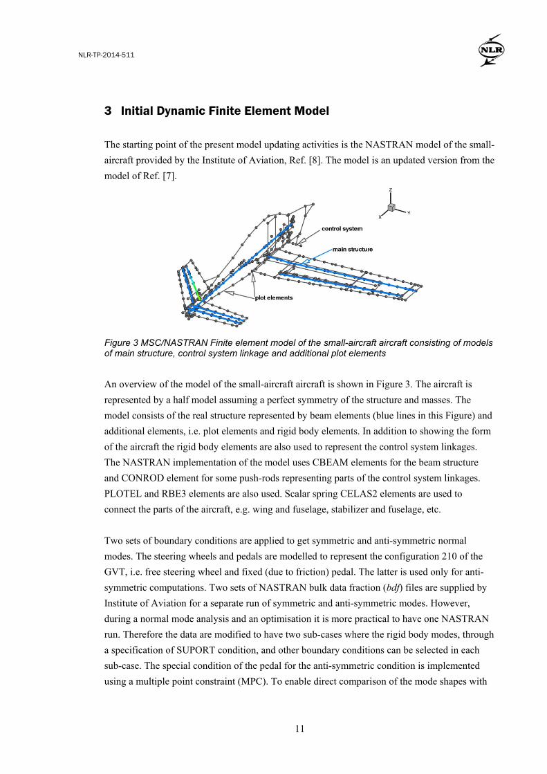
The starting point of the present model updating activities is the NASTRAN model of the small-aircraft provided by the Institute of Aviation, Ref. [8]. The model is an updated version from the model of Ref. [7].

Figure 3 MSC/NASTRAN Finite element model of the small-aircraft aircraft consisting of models of main structure, control system linkage and additional plot elements

An overview of the model of the small-aircraft aircraft is shown in Figure 3. The aircraft is represented by a half model assuming a perfect symmetry of the structure and masses. The model consists of the real structure represented by beam elements (blue lines in this Figure) and additional elements, i.e. plot elements and rigid body elements. In addition to showing the form of the aircraft the rigid body elements are also used to represent the control system linkages. The NASTRAN implementation of the model uses CBEAM elements for the beam structure and CONROD element for some push-rods representing parts of the control system linkages. PLOTEL and RBE3 elements are also used. Scalar spring CELAS2 elements are used to connect the parts of the aircraft, e.g. wing and fuselage, stabilizer and fuselage, etc. Two sets of boundary conditions are applied to get symmetric and anti-symmetric normal modes. The steering wheels and pedals are modelled to represent the configuration 210 of the GVT, i.e. free steering wheel and fixed (due to friction) pedal. The latter is used only for anti-symmetric computations. Two sets of NASTRAN bulk data fraction (bdf) files are supplied by Institute of Aviation for a separate run of symmetric and anti-symmetric modes. However, during a normal mode analysis and an optimisation it is more practical to have one NASTRAN run. Therefore the data are modified to have two sub-cases where the rigid body modes, through a specification of SUPORT condition, and other boundary conditions can be selected in each sub-case. The special condition of the pedal for the anti-symmetric condition is implemented using a multiple point constraint (MPC). To enable direct comparison of the mode shapes with

NLR-TP-2014-511

12

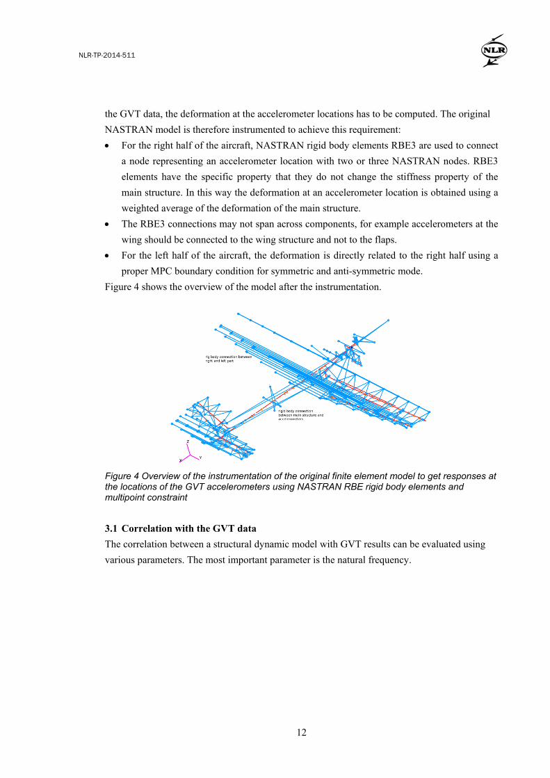
the GVT data, the deformation at the accelerometer locations has to be computed. The original NASTRAN model is therefore instrumented to achieve this requirement: • For the right half of the aircraft, NASTRAN rigid body elements RBE3 are used to connect

a node representing an accelerometer location with two or three NASTRAN nodes. RBE3 elements have the specific property that they do not change the stiffness property of the main structure. In this way the deformation at an accelerometer location is obtained using a weighted average of the deformation of the main structure.

• The RBE3 connections may not span across components, for example accelerometers at the wing should be connected to the wing structure and not to the flaps.

• For the left half of the aircraft, the deformation is directly related to the right half using a proper MPC boundary condition for symmetric and anti-symmetric mode.

Figure 4 shows the overview of the model after the instrumentation.

Figure 4 Overview of the instrumentation of the original finite element model to get responses at the locations of the GVT accelerometers using NASTRAN RBE rigid body elements and multipoint constraint

3.1 Correlation with the GVT data The correlation between a structural dynamic model with GVT results can be evaluated using various parameters. The most important parameter is the natural frequency.

NLR-TP-2014-511

13

Figure 5 Summary of the comparison of the natural frequencies between the GVT results and the initial FE model

Figure 5 presents the summary of the correlation between the natural frequencies computed using the initial NASTRAN model and the GVT data for the symmetric modes. The discrepancy in the natural frequencies is actually quite small, i.e. between 0% up to 9% for mode number 9, the aileron rotation mode. Slightly larger discrepancy in the natural frequency compared to the symmetric modes is observed, i.e. between 0% up to about 12% for mode 7. In general, however, the discrepancy is relatively small. It may be concluded that the initial model is actually quite good. Further model updating should be considered as a fine tuning of the initial model with respect to for example natural frequencies. Other correlation parameters are related to the mode shape. The most common parameter to compare the mode shape is the modal assurance criterion (MAC):

𝑀𝑀𝑀 =[𝜙𝐺𝜙𝐴 ]2

[𝜙𝐺𝑇𝜙𝐺][𝜙𝐴𝑇𝜙𝐴] (1)

where φ represents a mode shape (i.e. vector of displacement amplitudes responses at the locations of the GVT accelerometers), subscript G denotes GVT result and subscript A denotes result of analytical model. It can be seen that a MAC value does not depend on the magnitude of the individual modes since it is normalised by the magnitude of both modes.

NLR-TP-2014-511

14

Figure 6 Example of correlation between the results of initial NASTRAN model with the GVT data for a symmetric mode

Figure 7 Example of correlation between the results of initial NASTRAN model with the GVT data for an anti-symmetric mode

The value of MAC ranges from 0 for perfectly uncorrelated (orthogonal) and 1 for perfectly correlated mode shapes φG and φA. Figure 6 shows an example of mode shape correlation between the results computed using the initial NASTRAN model and the GVT data. All mode shapes are normalised such that the maximum deformation is 1 m. A high value of MAC is

NLR-TP-2014-511

15

obtained implying a very good correlation between the experiment and analytical model. This high value of MAC is also reflected in the lower part of the figure depicting good correspondence of the mode shapes. The high value of MAC does not have to be accompanied with a good correlation in the natural frequency. This is shown in Figure 7 depicting a correlation for an anti-symmetric mode. While the correlation of the mode shape is excellent, MAC=0.99, the discrepancy in the natural frequency is relatively large. In such cases the question may arise whether the correct modes are correlated, in particular if the natural frequency difference is very high. 3.2 Error localisation The lower part of the plots shown in Figure 6 and Figure 7 indicates the quality of the correlation in the aircraft structure for a certain mode. One can see directly locations where the correlation is good (e.g. the wings) or bad (e.g. the vertical tail). Such information can also be obtained for all modes by carrying out MAC computation along the modes for a node, the so-called coordinate MAC or COMAC. COMAC is defined as:

𝑀𝐶𝑀𝑀𝑀𝑖 = 1 −�∑ �𝜙𝐺,𝑛,𝑖 𝜙𝐴,𝑛,𝑖�𝑁

𝑛 �2

∑ �𝜙𝐺,𝑛,𝑖2 � ∑ �𝜙𝐴,𝑛,𝑖

2 �𝑁𝑛

𝑁𝑛

(2)

The subscript i indicates a node number or a location. The 1-minus definition has been traditionally defined to have a large value when the error is large and small value when the error is low. Since the summation runs over the modes the scaling of the mode-shape has to be the same. A sign difference between GVT and analytical model (180 degree phase difference) would influence the COMAC value. This is not the case for the MAC. The most common way to scale the mode-shape is by using the modal scale factor (MSF).

Figure 8 Example of scatter plot to determine the modal scale factor between a mode shape obtained from NASTRAN and the GVT data

NLR-TP-2014-511

16

Figure 8 shows an example of a scatter plot between the GVT data and the mode shapes obtained from the initial NASTRAN model for all degrees of freedom representing the unidirectional GVT accelerometers. The MSF is practically the factor that has to be applied to obtain a best-fit between these data.

Figure 9 COMAC values for the symmetric modes of the small-aircraft aircraft correlating the initial NASTRAN model and the GVT data

The computed COMAC data for the symmetric modes is plotted in Figure 9. The size of the dots at the accelerometer locations represents the COMAC value over all symmetric modes. It can be seen that the errors are reasonably well distributed. In some case, e.g. Ref.[10], the error location becomes obvious when the COMAC value at one location is much larger than the rest, pointing directly to the location where the model needs to be updated. It should be noted however, that in general a large value of COMAC at a location does not have to signify the exact location of the error, Ref.[10]. For example the COMAC data for the anti-symmetric modes shown in Figure 10 indicates a relatively large error at the flaps. Careful inspection reveals that the error is most likely not in the parameters of the flap beam elements but in the spring stiffness at the hinge.

Figure 10 COMAC value for the anti-symmetric modes of the small-aircraft aircraft correlating the initial NASTRAN model and the GVT data

A better error localisation method which focuses directly on the stiffness or mass error is the error matrix method (EMM), Ref. [10]. The essence of the method is the quantification of the

NLR-TP-2014-511

17

differences in the stiffness matrices reconstructed using the modes shapes and natural frequencies. This approach is not applied in the present work since it is more applicable for a very large finite element model.

NLR-TP-2014-511

18

Model updating procedure 4

The present model updating follows the computational model updating procedures. Starting from an initial model, the objective is to find the model parameters which improve the characteristics of the model to resemble the experimental data as closely as possible. It should be noted however, that the exercise is directed towards removing modelling inaccuracy. Results in the form of a mathematical model with less relation to the physics of the aircraft has to be avoided. The selected approach is to take advantage of the optimisation capability of NASTRAN. The design optimisation module of NASTRAN is usually applied to minimise a certain design objective, for example weight, for prescribed parameters such as element properties or even the geometry. The present approach uses the design optimisation module of NASTRAN to minimise the differences between the analytical model and the experiment. 4.1 Updating through optimisation To setup an optimisation process, an error function has to be defined which represent the differences between the analytical model and the experimental data. First, consider the vector or error in the natural frequency f as:

{𝜖} = �𝑓𝐴 − 𝑓𝐺𝑓𝐺

� (3)

The subscripts A and G represent the analytical model and the GVT data, respectively. The error {ε} is a function of the selected design parameters, i.e. parameters which may be modified during the optimisation process. An optimisation process can be setup to minimise this error by defining the objective function to be the sum of squared error as

𝐶 = {𝜖}𝑇{𝜖} (4)

The expressions given above are based on the implicit assumption that the errors are uncorrelated with each other and with the independent design parameters and moreover have equal variance. As generally known, experimental data may contain inaccuracies. In most cases, the inaccuracy varies between modes. Therefore it is more appropriate to express the minimisation problem with a weighted-squared sum type of objective function, where the following scalar objective function is minimised:

𝐶𝑇 = {𝜖}𝑇[𝑊𝑇]{𝜖} (5)

NLR-TP-2014-511

19

The weigh factor represented by matrix [WT] can be specified differently for each mode to reflect the confidence in the test data. It should be clear that a minimisation procedure using the aforementioned objective function OT does not take into account any consequences on the magnitude of the parameter change from the initial value. In some cases, the starting value of the design parameters, i.e. the initial analytical model, could already be good. As long as the value of the error is reduced, any modified parameter is always considered to be superior to the initial value, no matter what magnitude or sign of the change. This situation could lead to a mathematical model which may not be representative to the physics of the aircraft. In such case, usage of the model beyond the optimisation range would likely to give unsatisfactory results. Therefore, the commonly used approach of limiting the parameter change is used, see Ref. [15][16]. First define the change in the parameter value as:

{Δ𝑝} = �𝑝 − 𝑝0𝑝

� (6)

An additional weighted least square term to minimise the change of the parameter is added to objective function OT to arrive at:

𝐶 = {𝜖}𝑇[𝑊𝑇]{𝜖} + {Δ𝑝}𝑇[𝑊𝑃]{Δ𝑝} (7)

The weighting factor [WP] represents the confidence in the initial model. It should be set to a large value when confidence is high, and a low value in the case of high uncertainty. The new term can also be seen as a regularisation term to the objective function which is very useful when the gradient of the original objective function ∂OT/∂p is close to singular. Finally, the differences in the mode shapes between the analytical model and the GVT data can also be minimised by including the weighted MAC function as:

𝐶𝐷 = {𝜖}𝑇[𝑊𝑇]{𝜖} + {𝑊𝐷}𝑇 {1 −𝑀𝑀𝑀𝑅𝑅𝐷} + {Δ𝑝}𝑇[𝑊𝑃]{Δ𝑝}

(8)

It should be noted, that MACRED represents the MAC value in the objective function computed from a set of limited key nodes and not from the complete set of nodes. 4.2 Implementation in NASTRAN The implementation of the aforementioned optimisation procedure in NASTRAN is relatively straightforward. First, the design variables are selected and the side constraints are defined. The

NLR-TP-2014-511

20

following lines in the bdf file of NASTRAN define the Young modulus as a design variable which is allowed to change from 99% up to 101% during the optimisation. $ design variables generated from: struct_mat DESVAR 100001 MESTR001 1.00 0.99 1.01 $ PROPERTIES connected to DESVAR 100001 DVMREL1 110001 MAT1 1 E 100001 1.70+10

... The next example shows that a design variable can be connected to multiple element properties, in this case the bending stiffness at both ends of a beam. The side constrains show that the properties may change from 80% up to 120%. $ design variables generated from: ail_pbeam DESVAR 100004 I1AIL004 1.00 0.80 1.20 $ PROPERTIES connected to DESVAR 100004 DVPREL1 110004 PBEAM 3051 I1(B) 100004 1.576-3 DVPREL1 110005 PBEAM 3061 I1(A) 100004 1.576-3

... In the preceding examples the design variable is proportional to the element or material properties. In general it can be linear, quadratic, etc. To evaluate the objective function during the optimisation process, the characteristics of the modified model need to be examined. This is done through the so-called design responses. The following example show that three responses, designated with ID A006, A106, and A206, are extracted from mode number 6. The first response is the natural frequency and the last two responses are the mode shape at node 41 and 53, degree of freedom number 3 (z-translation). $ anti-symmetric response needed to form objective function DRESP1 120001 A006 FREQ 6 DRESP1 120002 A106 DISP 3 6 41 DRESP1 120003 A206 DISP 3 6 53

... Both design parameters and the design responses are used to define the objective function to be minimised, i.e. Equation (7). The following example shows the three components of the objective function: the error in the frequency, the 1-MAC function and the regularisation term. $ equation defining objective function DEQATN 120115 F(V001,V002,...,A418)=WT*(W006*((G006-A006)/G006)**2+ W014*((G014-A007)/G014)**2+W024*((G024-A008)/G024)**2+ ... +WD*(W006*(1.-(A106*G106+A206*G206+A306*G306+A406*G406)**2 /SSQ(A106,A206,A306,A406)/SSQ(G106,G206,G306,G406))+ ... +WP*(X001*(V001-1.0)**2+X002*(V002-1.0)**2+...

...

NLR-TP-2014-511

21

Finally, some other data including the frequency and mode shape from the GVT and other user inputs can be supplied through the use of NASTRAN table input, as shown in the following example. $ table of data from GVT and weighting factors DTABLE WT 900.00 WP 0.10 WD 100.00G006 7.740 G106 -0.098 G206 -0.081 G306 -0.036 G406 0.821 W006 1.000 G014 11.330 G114 0.032 G214 0.063 G314 0.035 G414 0.056 W014 1.000 G024 12.690

...

For a design optimisation run, the SOL 200 module of NASTRAN is used. The optimisation process in NASTRAN uses an approximate model to accelerate the process, see Figure 11. The default optimizer, used in the present work, is gradient-based and described in Refs. [17][18].

Figure 11 Schematic diagram of optimisation process implemented in NASTRAN, Ref. [14]

NASTRAN eigenvalue extraction during a SOL 200 run has a very useful feature called the mode tracking. The computed modes during subsequent updates of the parameters are ordered according to the initial numbering. This is done by using a cross-orthogonality check between the current and previous modes during design iterations. In this way the initial model can be used as a fixed reference.

NLR-TP-2014-511

22

Sensitivity study, parameter selection 5

It is generally known that a smart parameter selection contributes significantly to the success in a model updating. As a general rule, the following requirements are put forward in Ref. [13]:

(1) Selected parameters should include a region with modelling error, (2) The objective function should be sensitive to the selected parameters, and (3) The number of parameters should be relatively small.

For the first point, as shown in section 3.2, error localisation through COMAC data show a more distributed error than a specific location. Thus element properties in all parts should be considered as candidate for parameters. To satisfy the second point, a sensitivity study is carried out and is presented in the following paragraphs. Regarding the third point, the most common way to reduce the number of parameters is by clustering. Various clustering methods are studied in Ref. [10]. For a model updating activity which involves a large number of degrees of freedom, the application of an advanced clustering method is essential to make the problem tractable. The present work, however, deals with a model having a relatively small number of degrees of freedom. A relatively simple and straightforward strategy is therefore followed based on the sensitivity data.

Figure 12 Overview of sensitivity of the objective function to the parameters in the aircraft components

Since a gradient-based optimiser is used in NASTRAN, sensitivity data is automatically available. Sensitivity data can be requested during a SOL 200 run by running the execution only up to the gradient computation. Figure 12 presents the sensitivity data of the objective function with respect to all the parameters. The parameters are grouped per aircraft component. In each

NLR-TP-2014-511

23

aircraft component, three properties are shown in sequence: two bending-stiffnesses, lateral and normal, and one torsional stiffness. For example, it can be seen from Figure 12 that the objective function is not sensitive to the lateral bending stiffness of the fuselage. It is however sensitive to the vertical and torsional stiffness properties of the fuselage. Moreover, the sensitivity of the objective function to the vertical stiffness changes sign along the fuselage.

Figure 13 Overview of region with relatively small sensitivity of the objective function to the beam stiffness properties and therefore excluded from the optimisation process

The first filter to the selection of the parameters is removal of element properties to which the objective function is not sensitive. Figure 13 shows an example of the elements with stiffness property to which the objective function has a small sensitivity. The cut-off value has been selected to be conservatively low, i.e. 0.01% of the maximum value. The second approach to reduce the number of parameters is by grouping the element properties together when the neighbouring elements have the same sign. Figure 14 depicts the sign of the sensitivity of the objective function to the vertical stiffness properties of the beam elements.

Figure 14 Sign of the sensitivity of the objective function to the vertical stiffness of the beam elements

NLR-TP-2014-511

24

Confirming the observation made on Figure 12, sign changes indeed occur two times along the fuselage. Elements having the same sign should be put into one group. Inspecting other stiffness properties, for example the torsional stiffness of the beams, reveal only slightly different properties, see Figure 15 the torsional stiffness properties of the beam elements.

Figure 15 Sign of the sensitivity of the objective function to the torsional stiffness of the beam elements

NLR-TP-2014-511

25

Results 6

Results are presented for the model updating of the the small-aircraft aircraft in the GVT configuration. The rigid body modes with zero frequencies are excluded from the updating process. It is common to assume that the mass data has been carefully developed and usually contains less error than the stiffness data, Ref. [11][10] [13]. Therefore in the present work only the stiffness parameters will be included. Further, the following issues should be mentioned: • The GVT data are obtained for a full aircraft, i.e. both left and right parts, while the model

assumes a perfect symmetry of the aircraft. This means that the model can only represent perfect symmetric and anti-symmetric modes. The use of GVT mode shapes to compute the reduced MAC in the objective function is carried out in such a way that these effects are compensated.

• Structural damping is measured during the GVT. The analytical model, however, does not contain this parameter. It is assumed that the effect of the damping is low and can be neglected.

• In the GVT result reported in Ref.[4] the confidence regarding the accuracy of the measurement is not quantified. Therefore, the same weight factor for all modes is used.

• The design parameters consist of the Young modulus, the bending and torsional stiffness properties of the beam and the stiffness of the scalar springs.

In the following sections, results of model updating using all parameters will be presented followed by results using selected parameters. 6.1 Updating using all parameters The results using all parameters as independent design variables are now described. The total number of variables is about 800. For the first exercise, only the error in the frequency is included in the objective function, i.e. Equation (7). Figure 16 shows the overview of the natural frequencies before and after updating and the GVT data. It can be seen that correlation with the GVT data of almost all frequencies is improved. The reduction of the error can be clearly seen in Figure 17 for the anti-symmetric modes and Figure 18 for the symmetric modes. Moreover, the error in the frequency of modes which are not improved was already relatively small and after the updating remains relatively small. The values of the MAC are also presented in the right part of Figure 17 and Figure 18. Inspecting Figure 17 and Figure 18 carefully, it can be seen that for some modes, the value of MAC decreases. This means that the correlation in the mode shape deteriorates even when the correlation of the frequency improves. Therefore the second exercise is carried out, now including the reduced MAC in the objective function, i.e. Equation (8).

NLR-TP-2014-511

26

Figure 16 Overview of natural frequencies before and after updating for symmetric and anti-symmetric modes. Optimisation using all element properties as parameters

The reduced-MAC in the objective function is computed using the mode shape data at four locations which are judiciously selected at the leading edge of the right wing-tip (accelerometer number 41), at the right aileron (accelerometer number 53), at the right flap (accelerometer number 62) and at the leading edge of the right wing measuring lateral bending of the wing (accelerometer number 50). The result of the optimisation is given in Figure 19. Comparing this with Figure 16 one can see that the improvement in the frequency correlation is not as good as in the case of minimising only the frequency error. However, the values of the MAC, presented in Figure 20, have indeed improved. To further investigate these contradictory effects several other optimisation processes are carried out with varying weighting factors for the frequency error [WT] and mode shape error [WD]. The results in terms of the error in the natural frequencies and the error in the mode shapes are shown in Figure 21. A monotonic trend is observed for both symmetric and anti-symmetric modes. A multi-objective optimisation study is a more appropriate approach for this type of problem but it is left for future activities. 6.2 Updating using parameter grouping To reduce the number of design variables, parameter grouping is carried out. First of all, the parameters to which the objective function has a small sensitivity are excluded. Subsequently, optimisation with design parameters grouped according to the aircraft component is carried out. Finally, the parameter groups are modified to respect the sign change of the sensitivity as described in the previous chapter. For the first parameter grouping, i.e. according to the aircraft components, the number of design variables reduces dramatically from 800 to just 48. The results of the updating are presented in

NLR-TP-2014-511

27

Figure 22. It can be seen that evenly good results are obtained as in the case of updating using all parameters, while the computing time is reduced to only about 10% of the updating process using all available parameters as design variables. Finally, results obtained using component-wise parameter grouping which respects the sign change of the sensitivity is shown in Figure 23. A small improvement can be observed for the 10th anti-symmetric mode only. The number of design variables for this parameter grouping is 44. It can therefore be mentioned that a straightforward component-wise parameter grouping is a good option to reduce the number of parameters.

Figure 17 Overview of errors in natural frequencies before and after updating for anti-symmetric modes. Optimisation using all element properties as parameters

Figure 18 Overview of errors in natural frequencies before and after updating for symmetric modes. Optimisation using all element properties as parameters

NLR-TP-2014-511

28

Figure 19 Overview of natural frequencies before and after updating for symmetric and anti-symmetric modes. Optimisation using all element properties as parameters; including the reduced MAC in the objective function

Figure 20 Overview of errors in natural frequencies before and after updating for symmetric modes and the MAC values. Optimisation using all element properties as parameters; including the reduced MAC in the objective function

NLR-TP-2014-511

29

Figure 21 Behaviour of error in natural frequencies and error in MAC for three different weighting factors

Figure 22 Overview of natural frequencies before and after updating for symmetric and anti-symmetric modes. Optimisation using component-wise grouping of the element properties as parameters

NLR-TP-2014-511

30

Figure 23 Overview of natural frequencies before and after updating for symmetric and anti-symmetric modes. Optimisation using component-wise grouping of the element properties as parameters while respecting the sign change in the sensitivity

Figure 24 Overview of the differences in vertical stiffness property of the beams between the updated model and the initial model. Small differences imply that the initial model is already accurate. Optimisation using all element properties as parameters

NLR-TP-2014-511

31

Figure 25 Overview of the differences in lateral stiffness property of the beams between the updated model and the initial model. Slightly larger differences are observed compared to the vertical stiffness property. Optimisation using all element properties as parameters

NLR-TP-2014-511

32

Conclusions 7

Successful model updating of the small-aircraft structural dynamic model based on the GVT data has been presented. An automatic updating method using an optimisation procedure is employed. For the analysis and optimisation, MSC/NASTRAN has been used instead of a specialised model updating software. The advantage is that the approach presented here requires only the MSC/NASTRAN software, which is assumed to be widely available to small aircraft industries. The definition of the objective function to minimise the difference in natural frequency and the difference in the mode shape has been studied. A method to select parameters has also been described and implemented. Based on the results and the experience gained during the course of the work the following conclusions may be drawn: (1) Improvement of the natural frequency error can be obtained for almost all modes. The

average relative error in the natural frequencies decrease from 3.8% to 1.4% for the anti-symmetric modes and from 1.9% to 1.5% for the symmetric modes. The variance has also been reduced implying a better overall accuracy. Note that the error of the modes which are not improved was already very low.

(2) The implementation of the updating procedure in NASTRAN is relatively straightforward, and requires no specialised model updating software.

(3) Optimisation using all available parameters, i.e. about 800 parameters, as design variables and using careful parameter grouping, which reduces the design variables to about 40, resulted in similar improvement. The computing cost for the optimisation using parameter grouping is about 90% lower. The significant reduction of computing time is useful when various optimisation strategies are going to be studied, e.g. different weighting factors, etc.

(4) To reduce the number of design parameters, a straightforward component-wise grouping is a good option next to a parameter grouping which respects the sign change of the sensitivity of the objective function to the parameters.

(5) Improvement of the natural frequency seems to reduce the MAC correlation of the modes leading to a suggestion that a multi-objective optimisation should be carried out.

Finally, the following recommendations are offered for future research: (1) Although provision has been made in the optimisation procedure to include both confidence

in the test data and confidence in the initial model, only a default value (the same for all modes) has been used. A study on the quantification of this aspect should be carried out.

(2) Optimisation in the sample nodes used for computing reduced MAC in the objective function should be carried out.

(3) Multi-objective optimisation should be carried out regarding minimising the error in the natural frequency and the error in the mode-shapes.

NLR-TP-2014-511

33

Acknowledgement

This research was partly funded by the EU through the ESPOSA project (GA/Nr.: ACP1-GA-2011-284859) and the FP6-CESAR project (GA/Nr.: AIP5-CT-2006-030888). References

[1] Böswald, M., Cecrdle, J., Report on Base Model Definition for Aeroelastic Analysis and Experiment, CESAR Report

[2] Mottershead, J.E. and Friswell, M.I. Model updating in structural dynamics: a survey. Journal of Sound and Vibration. vol. 167, pp. 347-375, 1993.

[3] E. Dascotte, Model Updating for Structural Dynamics: Past, Present and Future Outlook. Presented at International Conference on Engineering Dynamics (ICED), April 16-18, 2007, Carvoeiro, Algarve, Portugal.

[4] Szymaniak, M. and Lorenc, Z. Ground Vibration Test of the small-aircraft Airplane. Technical Report 62/BW-W3/98. Laboratory of Strength and Dynamics, Institute of Aviation, 1998.

[5] European Aviation Safety Agency, CS-23 - Certification Specifications for Normal, Utility, Aerobatic and Commuter Category Aeroplanes, ED Decision 2003/14/RM

[6] Federal Aviation Administration, Means of Compliance with Title 14 CFR, Part 23, § 23.629, Flutter, AC No: 23.629-1B

[7] Chajec, W., Aeroelastic Reference Model of the small-aircraft. Flutter Calculation based on GVT results, Institut Lotnictwa Warszawa

[8] Chajec, W., Aeroelastic Reference Model of the small-aircraft. Control Surface System Modeling Adding into the Beam-like Model in MSC NASTRAN, Institut Lotnictwa Warszawa

[9] CESAR TASK 2.5 partners, Halftime report on improved methods for reliable and fast prediction of aeroelastic stability and on optimized analytical and experimental approaches and methods, CESAR Report.

[10] Hatch, C., Skingle, G.W., Greaves, C.H., Lieven, N.A.J., Coote, J.E., Friswell, M.I., Mottershead, J.E., Shaverdi, H., Mares, C., McLaughlin, A., Link, M., Piet-Lahanier, N., Van Houten, M.H., Göge and D., Rottmayr, H. (2006) Methods for Refinement of Structural Finite Element Models: Summary of the GARTEUR AG14 Collaborative Programme. In: 32nd European Rotorcraft Forum, 2006, Maastricht, The Netherlands (Europe).

[11] Göge, D. Automatic updating of large aircraft models using experimental data from ground vibration testing. Aerospace Science and Technology. vol. 7, pp 33-45, 2003.

[12] Kim, G.-H. and Park, Y. An automated parameter selection procedure for finite element model updating and its applications. Journal of Sound and Vibration. vol. 309, pp 778-793, 2008.

[13] Friswell, M.I. and Mottershead, J.E. Finite Element Model Updating in Structural Dynamics. Kluwer Academic Publisher, London, 1995.

[14] Johnson, E. Design Sensitivity and Optimization User’s Guide of MSC.Nastran 2005 r3. MacNeal Schwendler Software Corporation. 2005.

[15] Collins, J.D., Hart, G.C., Hasselman, T.K. and Kennedy, B. Statistical Identification of Structures. AIAA Journal. vol. 12 pp. 185-190. 1974.

NLR-TP-2014-511

34

[16] Blakely, K. Matching frequency response test data with MSC/NASTRAN. NASTRAN World User Conference. 1994.

[17] Vanderplaats, G. N., “ADS -- A FORTRAN Program for Automated Design Synthesis -- Version 1.10,” NASA Contractor Report 177985, NASA Langley Research Center, Hampton, Virginia, 1985.

[18] DOT, Design Optimization Tools, User Manual, Version 5, Vanderplaats Research and Development, Inc., Colorado Springs, CO, 1999.