RESEARCH ARTICLE10.1002/2015JC011226

Modeled sensitivity of the Northwestern Pacific upper-oceanresponse to tropical cyclones in a fully coupled climate modelwith varying ocean grid resolutionHui Li1, Ryan L. Sriver1, and Marlos Goes2,3

1Department of Atmospheric Sciences, University of Illinois at Urbana-Champaign, Urbana, Illinois, USA, 2CooperativeInstitute for Marine and Atmospheric Studies, University of Miami, Miami, Florida, USA, 3NOAA/AOML, PhysicalOceanography Division, Miami, Florida, USA

Abstract Tropical cyclones (TCs) actively contribute to Earth’s climate, but TC-climate interactions arelargely unexplored in fully coupled models. Here we analyze the upper-ocean response to TCs using a high-resolution Earth system model, in which a 0.58 atmosphere is coupled to an ocean with two different hori-zontal resolutions: 18 and 0.18. Both versions of the model produce realistic TC climatologies for the North-western Pacific region, as well as the transient surface ocean response. We examined the potentialsensitivity of the coupled modeled responses to ocean grid resolution by analyzing TC-induced sea surfacecooling, latent heat exchange, and basin-scale ocean heat convergence. We find that sea surface coolingand basin-scale aggregated ocean heat convergence are relatively insensitive to the horizontal ocean gridresolutions considered here, but we find key differences in the poststorm restratification processes relatedto mesoscale ocean eddies. We estimate the annual basin-scale TC-induced latent heat fluxes are1.70 6 0.16 3 1021 J and 1.43 6 0.16 3 1021 J for the high-resolution and low-resolution model configura-tions, respectively, which account for roughly 45% of the total TC-induced ocean heat loss from the upperocean. Results suggest that coupled modeling approaches capable of capturing ocean-atmosphere feed-backs are important for developing a complete understanding of the relationship between TCs and climate.

1. Introduction

Increasing evidence suggests TCs play an active role in influencing the dynamics of the coupled ocean-atmosphere system [Emanuel, 2001; Hart, 2011; Sriver et al., 2008, 2010; Sriver and Huber, 2007]. Severalrecent studies have shown that enhanced upper-ocean mixing, associated with extreme TC winds, couldlead to positive ocean heat convergence (OHC) [Bueti et al., 2014; Emanuel, 2001; Jansen et al., 2010; Meiet al., 2013; Mei and Pasquero, 2012; Park et al., 2011; Sriver, 2013; Sriver et al., 2010; Sriver and Huber, 2007],which may potentially alter large-scale circulations and transports of the ocean-atmosphere system [Booset al., 2004; Emanuel, 2001; Hu and Meehl, 2009; Jansen and Ferrari, 2009; Pasquero and Emanuel, 2008; Sriverand Huber, 2010]. These TC processes and feedbacks are generally not captured in current numerical modelsused for climate projections, but their representation may be necessary to reduce uncertainty in projectionsof climate change impacts.

Numerical models are useful tools to explore the relationship between TCs and climate. Many uncoupledatmosphere and ocean modeling experiments have pointed to important climate connections associatedwith TCs. High-resolution atmosphere models have demonstrated skill in simulating realistic TC-like circula-tions and basin-scale climatologies, and they have been used to examine the sensitivity of TC activity to pre-scribed changes in climate [Bacmeister et al., 2013; Camargo et al., 2005; Wehner et al., 2010], and increasingatmosphere model grid resolution can significantly improve the representation of simulated TCs [Bacmeisteret al., 2013; Li et al., 2013; Manganello et al., 2012; Murakami and Sugi, 2010; Strachan et al., 2012; Walshet al., 2013; Wehner et al., 2014]. In addition to atmosphere-only experiments, ocean-only models have beenused extensively to analyze the oceanic response to TC forcing, including TC influences on ocean heat con-vergence [Jansen and Ferrari, 2009; Vincent et al., 2013], mixing budgets [Huang et al., 2009; Mei and Pas-quero, 2012], and large-scale ocean heat transport and circulations [Bueti et al., 2014; Jansen and Ferrari,2009; Jullien et al., 2012; Sriver et al., 2010; Sriver and Huber, 2010; Vincent et al., 2013; Wang et al., 2014].

Key Points:� The upper-ocean responses to TCs

are analyzed in a high resolution fullycoupled climate model� High resolution coupled model is

capable of simulating realistic TC-induced upper ocean responses� Tropical cyclones can influence upper

ocean mixing and heat budgets inthe coupled model

Supporting Information:� Supporting Information S1

Correspondence to:H. Li,huili7@illinois.edu

Citation:Li, H., R. L. Sriver, and M. Goes (2016),Modeled sensitivity of theNorthwestern Pacific upper-oceanresponse to tropical cyclones in a fullycoupled climate model with varyingocean grid resolution, J. Geophys. Res.Oceans, 121, 586–601, doi:10.1002/2015JC011226.

Received 12 AUG 2015

Accepted 15 DEC 2015

Accepted article online 18 DEC 2015

Published online 21 JAN 2016

VC 2015. American Geophysical Union.

All Rights Reserved.

LI ET AL. OCEAN RESPONSE TO TCs IN COUPLED MODEL 586

Journal of Geophysical Research: Oceans

PUBLICATIONS

Ocean-atmosphere coupling is important for quantifying surface fluxes of heat and momentum withinstorm-affected regions [Bender and Ginis, 2000; Jullien et al., 2014], as well as potential remote impacts asso-ciated with altered dynamics [Bender and Ginis, 2000; Jullien et al., 2014; Pasquero and Emanuel, 2008; Scocci-marro et al., 2011]. Several recent modeling studies have shown that coupled climate models are capable ofsimulating present-day TC statistics, including geographical distribution, frequency, and interannual variabil-ity [Bell et al., 2013; Gualdi et al., 2008; Kim et al., 2014; Rathmann et al., 2014]. These models typically exhibitbiases across different basins due to their generally coarse model resolution, relatively short simulationtimes, and/or uncertainties related to integrated model responses and interactions. Coupled climate modelshave also been used to explore potential TC connections to large-scale climate features. For example, Huand Meehl [2009] use a relatively coarse resolution (�2.88 atmosphere �18 ocean) version of the CommunityClimate System Model (CCSM), to explore the effect of TCs on meridional volume and heat transports, find-ing that the positive influence of TC-induced diapycnal ocean mixing on meridional transports is partiallymodulated by increased freshwater forcing associated with heavy TC precipitation. Also using a relativelylow-resolution version of CCSM3, Manucharyan et al. [2011] analyzed how imposed intermittent verticalocean mixing associated with TC events may affect large-scale ocean temperature structure and circulationpatterns. They found that the additional TC-like mixing leads to both enhanced poleward ocean heat trans-port and tropical equatorial heat convergence. Scoccimarro et al. [2011] investigated the North Hemispherepoleward ocean heat transport induced by model-generated TCs on both transient and long-term timescales with a 0.758 atmosphere and 28 ocean. They concluded that TCs could largely enhance the oceanheat transport on weekly time scales, but the effect is negligible when considering annually averaged oceanheat transport.

These past studies have provided fundamental insights into the potential relationship between TCs and cli-mate, but they are generally limited by relatively coarse ocean grid resolution and a lack of appropriateocean-atmosphere coupling for analyzing TC effects in the coupled system. While several studies [e.g.,Wehner et al., 2014] have investigated the effects of increased atmosphere resolution on TC climatologies,the sensitivity of the upper-ocean response to ocean grid resolution has not been adequately addressedwithin coupled model frameworks. Here we analyze the upper-ocean response to TCs using a high-resolution configuration of the Community Climate System Model version 3.5 (CCSM 3.5) [Kirtman et al.,2012], which features an atmosphere model with 0.58 horizontal resolution coupled to an ocean model withtwo different horizontal resolutions (18 and 0.18). This model is capable of simulating realistic TC circulationsand cold wakes (Figure 1), as well as TC-induced subsurface thermocline warming [McClean et al., 2011]. Weuse the results of the model experiments to analyze TC climatologies, the transient upper-ocean response

Figure 1. (a) Simulated TC circulation using CCSM3.5 with a 0.58 atmosphere model. (b) The corresponding surface temperature anomalyfrom the 0.18 eddy-resolving ocean component. The temperature anomaly is estimated as the poststorm minus prestorm temperaturefields.

Journal of Geophysical Research: Oceans 10.1002/2015JC011226

LI ET AL. OCEAN RESPONSE TO TCs IN COUPLED MODEL 587

to TC passage, and basin-scale aggregated TC effects on ocean heat convergence and surface heat fluxes.We focus our analysis on the Northwestern Pacific Ocean, which represents a region exhibiting a realistic TCclimatology and seasonal variability within both model configurations. A key goal of this paper is to exam-ine the potential sensitivity of the coupled modeled response to increasing ocean grid resolution towardscales capable of resolving mesoscale ocean eddies.

This paper is organized as follows. Section 2 describes the model, observational data, TC tracking scheme,and methods for the OHC calculations. Section 3 is the main results section, which is divided into threeparts. We first analyze and compare the modeled TC climatologies of the two model configurations. Wethen investigate the sensitivity of surface responses, including surface cooling and latent heat fluxes, toocean grid resolution. In particular, the sensitivities are further examined by analyzing potential effects ofparameterized versus resolved mesoscale ocean eddies. Lastly, we show first-order estimates of the basin-scale annual mean TC-induced latent heat budget and ocean heat convergence within the coupled model.The caveats of this study are discussed in section 4. The main conclusions and implications of this work aresummarized in section 5.

2. Data and Methods

2.1. Model DescriptionWe analyze model output from a set of century-scale present-day control simulations using high-resolutionconfigurations of CCSM 3.5 [Gent et al., 2010; Kirtman et al., 2012; McClean et al., 2011]. CCSM3.5 is a prere-lease version of CCSM4 and includes the Community Atmospheric Model (CAM) version 3.5 [Gent et al.,2010] coupled to the Parallel Ocean Program (POP) version 2 [Danabasoglu et al., 2012; Gent et al., 2010].The modeling experiment consists of two simulations in which the 0.58 atmosphere component model iscoupled to two different versions of the ocean model. The low-resolution control simulation features oceanand sea-ice components with a nominal 18 horizontal resolution, with constant grid spacing in the zonaldirection (1.28) and varying grid spacing in the meridional direction (0.278 at the equator to 0.548 in the mid-latitudes). The high-resolution control simulation features ocean and sea-ice components with a uniform0.18 horizontal spacing at the equator, and reducing to �0.028 at high latitudes. Both ocean model versionshave 42 vertical levels with thickness varying from 10 m at the surface to 250 m at 6000 m depth. Momen-tum and heat fluxes at the air-sea interface are computed by the coupler and are shared among modelcomponents. Surface wind stress is calculated using relative wind, which refers to the difference betweenlowest model level wind and ocean current velocities. Ocean vertical mixing is parameterized using K-profile parameterization (KPP) scheme. Kirtman et al. [2012] find that small-scale features resolved in thehigh-resolution ocean model (e.g., mesoscale eddies) can alter large-scale climate conditions, such as globalmean temperature, general circulation patterns, Arctic sea ice losses, rainfall, ocean stratification, climatevariability, and air-sea interactions.

The simulations include over 100 years of monthly output from the ocean and atmosphere models, ofwhich roughly 20 years of output also include a subset of daily surface variables. We focus our analysis pri-marily on the 20 years of daily surface output for analyzing the transient TC effects. Available daily variablesfrom the model simulations include surface wind stress, surface temperature, surface latent and sensibleheat fluxes, and precipitation rate. The daily model output does not contain any subsurface ocean variables.Our analysis is limited by the lack of daily subsurface ocean information; however, the available atmospheresurface outputs enable us to perform comprehensive sensitivity analyses of the transient TC-inducedresponses near the ocean-atmosphere interface. In addition, we analyze basin-scale TC-induced ocean heatbudgets using previously published methods that combine daily surface temperature information withmonthly vertical temperature profiles [Sriver et al., 2008] (see section 2.4), which are available for these simu-lations. These methods have been shown to provide robust first-order estimates of transient ocean heatuptake compared to altimetry-based estimates [Mei et al., 2013]. Note that such methods may overestimatethe ocean heat uptake considering the importance of the variations in the prestorm stratification [Vincentet al., 2012b], vertical advection [Jullien et al., 2012], and thermocline seasonal variations [Jansen et al.,2010]. These limiting assumptions provide important constraints on the first-order estimates of surfacefluxes and ocean heat convergence.

Journal of Geophysical Research: Oceans 10.1002/2015JC011226

LI ET AL. OCEAN RESPONSE TO TCs IN COUPLED MODEL 588

2.2. Tropical Cyclone Detection and Tracking AlgorithmWe developed an algorithm to identify TC-like circulations in the model. The algorithm is adapted from pre-vious studies analyzing TCs in atmosphere-only simulations [Camargo and Zebiak, 2002; Zhao et al., 2009],based on the availability of daily variables outlined in section 2.1. We identify a TC-like circulation within themodel using the following criteria: (1) cyclogenesis occurs within 308 of the equator; (2) the maximum sur-face wind stress curl exceeds 2 3 1026 N m23, and maximum 10 m wind speed exceeds 15 m s21 corre-sponding to a relaxed threshold for the minimum wind speed for a tropical storm; (3) the horizontal scale islarger than 200 km; (4) the storm center must not be stationary for more than 24 h; and (5) the event mustlast for at least 3 days. Criteria (3) and (4) are important constraints to filter standing ocean eddies, since weare using relative wind (differences between 10 m wind and ocean current) derived from surface windstress as the basis for constructing TC surface wind fields. Several of our criteria are consistent with previousTC detection methods [Camargo and Zebiak, 2002; Zhao et al., 2009], however, some differences are neces-sary given the limited number of variables available from the model output. For example, maximum surfacewind stress curl is used to identify and locate a potential TC storm center, rather than the 850 hPa vorticityand minimum sea level pressure. In addition, the cyclone core structure is not considered here. We haveperformed multiple sensitivity tests to optimize the detection and tracking algorithms and we calibrate thethreshold values for each variable. Results are visually inspected to ensure the characteristics of the identi-fied circulations are consistent with TC events (Figure 1). Additional details about the procedure can befound in supporting information.

2.3. Observational DataWe use the Optimally Interpolated Sea Surface Temperature (OI SST) data product to analyze observed TC-induced near-surface ocean temperature responses. The OI SST is a hybrid product of the Tropical RainfallMeasuring Mission’s (TRMM) Microwave Imager (TMI) and the Advanced Microwave Scanning Radiometer(AMSRE) data, which provides complete daily SST at 0.258 horizontal resolution from 2002 to present [Gente-mann et al., 2010]. We analyze all TCs globally between 2003 and 2012 as defined by the best track data set,which combines track information from NOAA’s Storm Prediction Center and the U.S. Navy’s Joint TyphoonWarning Center. The best track product categorizes TC tracks within five different regions: North Atlantic,East Pacific, West Pacific, Indian Ocean, and Southern Hemisphere. We analyze subsurface ocean propertiesusing potential temperature profiles and mixed-layer depths from the European Center for Medium-RangeWeather Forecast Ocean Reanalysis System 4 (ECMRWF ORAS4), providing monthly ocean state informationbetween 1957 and present. Climatological mixed-layer depth and SST in ORAS4 are compared with thatfrom the World Ocean Atlas 2013 (WOA13) [Locarnini et al., 2013] to ensure validity of this data set (support-ing information Figures S5–S8). Annually and seasonally averaged observational wind data are fromNational Center for Climate Prediction/National Center for Atmospheric Research (NCEP/NCAR) reanalysis.Monthly averaged eddy kinetic energy (EKE) is derived from 17 years (1993–2010) of monthly averaged seasurface height anomalies (SSA) [Le Traon et al., 1998], produced by Ssalto/Duacs and distributed by Aviso.The data are a gridded 1/48 3 1/48 global product merged from several altimeter satellite missions. The sealevel anomalies are referenced to a 20 year period (1993–2012).

2.4. Calculation of TC-Induced Ocean Heat Convergence (OHC)The TC-induced, vertically integrated OHC is estimated following previous methods [Emanuel, 2001; Sriveret al., 2008; Sriver and Huber, 2007]:

OHC5

ð ð ðFDTdhdWdL; (1)

where F is the fraction of heat transported downward through the base of the oceanic mixed layer throughmixing and entrainment, DT is the magnitude of surface temperature anomaly, dh is the depth of verticalmixing, and dW and dL are the cross-track and along-track length of the storm wake. Seawater density qand heat capacity C are held constant at 1020 kg/m3 and 3900 J/(kg 8C), respectively. In order to estimate F,we analyze surface latent heat exchange during TC days, as it is the second largest contributor to sea sur-face cooling [Huang et al., 2009] (see section 3.3). We employ a footprint method that samples surface prop-erties within a 68 3 68 domain (dW and dL), which is centered on the best track location and moves withthe storm. The footprint domain size is consistent with area sizes used in other studies [Cheng et al., 2014;Lloyd and Vecchi, 2011; Mei and Pasquero, 2012; Sriver and Huber, 2007]. At each storm location, temperature

Journal of Geophysical Research: Oceans 10.1002/2015JC011226

LI ET AL. OCEAN RESPONSE TO TCs IN COUPLED MODEL 589

anomalies are calculated using SST from 2 days after storm passage relative to the average SST between 12and 5 days prior to the storm. Sensitivity analyses were performed to choose characteristic sizes of the foot-print domain and time interval, and we chose values that maximized the TC effect. The results presentedhere are generally insensitive to the choice of spatial and temporal sampling scales, particularly for the com-parison between model simulations with varying ocean grid resolution.

We use three different strategies for estimating TC-induced mixing depths that we apply to both modelsimulations and observations. First, we assume a uniform and constant mixing depth of 50 m, consistentwith past case study analysis [D’Asaro et al., 2007] and methods used in previous observation-based studies[Sriver and Huber, 2007]. For the second method, we assume that vertical mixing for all storms penetrates tolevels corresponding to the monthly climatological mixed-layer depth at each grid point. In the thirdmethod, we combine the TC-induced SST anomalies with monthly climatological vertical ocean tempera-ture profiles to estimate mixing depth as the level from which water must be upwelled to achieve theobserved surface temperature anomaly [Sriver et al., 2008]. In this method, mixing depth is calculated asdh5DT � @z=@T , where DT is the TC-induced SST anomaly and @z=@T is the inverse of the vertical tempera-ture gradient obtained from the monthly climatological ocean temperature at each location. All three meth-ods likely underestimate the actual TC-induced vertical mixing length scale, but we chose these criteria inorder to examine the robustness of the model’s response and resolution dependence under uncertainassumptions. Ocean heat convergence on each grid point is then calculated individually before being inte-grated across the footprint domain, to account for any nonuniform cooling anomalies within the domain.

3. Model Results and Discussion

3.1. Modeled Tropical Cyclone Number and ClimatologyTC tracks accumulated over 20 years in both versions of the model are shown in Figures 2a and 2b. We findthat both the low-resolution and high-resolution simulations generally capture the spatial distribution of theglobal storm tracks. However, both model configurations exhibit several key limitations. The total number ofstorms globally is roughly 50% of the observed current-day climatology (Table 1). The annual TC counts inthe north Atlantic and east Pacific basins are too low compared to observed climatologies (Figure 3). For the

Figure 2. Model-simulated storm tracks accumulated over 20 years in the (a) low-resolution and (b) high-resolution configurations. Mod-eled annually accumulated, storm-induced average sea surface cooling for the (c) low-resolution and (d) high-resolution configurations.

Journal of Geophysical Research: Oceans 10.1002/2015JC011226

LI ET AL. OCEAN RESPONSE TO TCs IN COUPLED MODEL 590

north Atlantic region, the bias may beattributed to relatively low annual SST(supporting information Figure S1) andrelatively high vertical wind shear (sup-porting information Figure S2) within theMain Development Region for both sim-ulations, which are both important envi-

ronmental factors for TC development. The model also simulates storms in the South Atlantic basin, whichare rarely observed in nature. The cause may be due to anomalously low vertical wind shear and warm SSTin this region compared to observations (supporting information Figures S1 and S2).

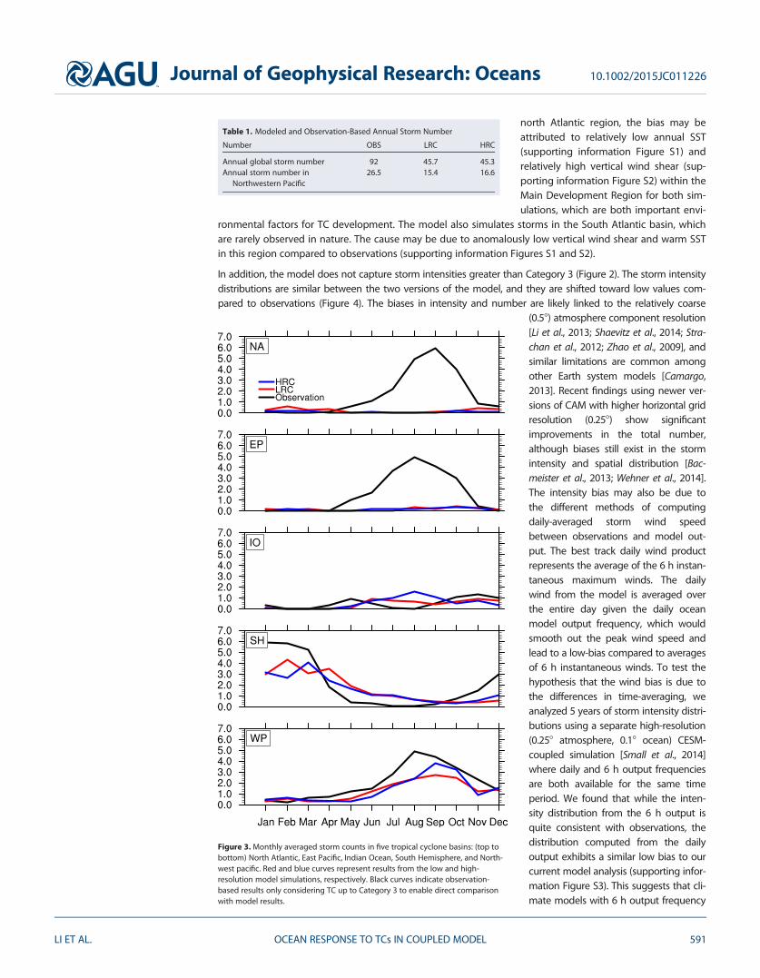
In addition, the model does not capture storm intensities greater than Category 3 (Figure 2). The storm intensitydistributions are similar between the two versions of the model, and they are shifted toward low values com-pared to observations (Figure 4). The biases in intensity and number are likely linked to the relatively coarse

(0.58) atmosphere component resolution[Li et al., 2013; Shaevitz et al., 2014; Stra-chan et al., 2012; Zhao et al., 2009], andsimilar limitations are common amongother Earth system models [Camargo,2013]. Recent findings using newer ver-sions of CAM with higher horizontal gridresolution (0.258) show significantimprovements in the total number,although biases still exist in the stormintensity and spatial distribution [Bac-meister et al., 2013; Wehner et al., 2014].The intensity bias may also be due tothe different methods of computingdaily-averaged storm wind speedbetween observations and model out-put. The best track daily wind productrepresents the average of the 6 h instan-taneous maximum winds. The dailywind from the model is averaged overthe entire day given the daily oceanmodel output frequency, which wouldsmooth out the peak wind speed andlead to a low-bias compared to averagesof 6 h instantaneous winds. To test thehypothesis that the wind bias is due tothe differences in time-averaging, weanalyzed 5 years of storm intensity distri-butions using a separate high-resolution(0.258 atmosphere, 0.18 ocean) CESM-coupled simulation [Small et al., 2014]where daily and 6 h output frequenciesare both available for the same timeperiod. We found that while the inten-sity distribution from the 6 h output isquite consistent with observations, thedistribution computed from the dailyoutput exhibits a similar low bias to ourcurrent model analysis (supporting infor-mation Figure S3). This suggests that cli-mate models with 6 h output frequency

Figure 3. Monthly averaged storm counts in five tropical cyclone basins: (top tobottom) North Atlantic, East Pacific, Indian Ocean, South Hemisphere, and North-west pacific. Red and blue curves represent results from the low and high-resolution model simulations, respectively. Black curves indicate observation-based results only considering TC up to Category 3 to enable direct comparisonwith model results.

Table 1. Modeled and Observation-Based Annual Storm Number

Number OBS LRC HRC

Annual global storm number 92 45.7 45.3Annual storm number in

Northwestern Pacific26.5 15.4 16.6

Journal of Geophysical Research: Oceans 10.1002/2015JC011226

LI ET AL. OCEAN RESPONSE TO TCs IN COUPLED MODEL 591

exhibit more accurate TC intensity distributionswhen comparing model output with best trackdata. Despite these biases, we find the CCSM3.5model captures the observed seasonal variability inseveral key basins (see Figure 3), including theNorthwestern Pacific region, which is where wefocus our analysis.

The consistency in storm intensity distributionsuggests that both versions of the model repre-sent similar climatological environmental condi-tions important for TC intensity. The effect ofprestorm SST is of particular interest here, since itmay be sensitive to the representation of meso-scale eddies. In order to diagnose the sensitivityof prestorm SST to model resolution, we analyzedthe frequency distribution of SST anomalies 3days prior to storm passage for all storm days(supporting information Figure S4). The anoma-lies are referenced to daily climatological values.The results show no significant difference in thedistributions, suggesting that eddies do not havea major impact on prestorm SST conditions in themodel.

3.2. Modeled TC-Induced Sea SurfaceResponses3.2.1. Spatial and Temporal Characteristics ofSea Surface CoolingThe annual averages of the accumulated TC-induced temperature anomalies for each versionof the model are shown in Figures 2c and 2d.Both model versions exhibit spatial patterns ofcooling that are consistent with previousobservation-based analyses [Sriver et al., 2008;Sriver and Huber, 2007]. The magnitude of the

accumulated TC-induced surface cooling in the model is generally lower compared to observations, whichis due primarily to the model’s underrepresentation of the TC number and intensity. In addition, the mod-eled surface temperature response is generally insensitive to horizontal ocean grid resolution, and thebiases are minimal in the Northwestern Pacific region.

In order to diagnose the transient response of upper-ocean temperature to TC passage, we analyze timeseries composites of the area-averaged SST anomalies for the low-resolution and high-resolution simula-tions (Figure 5). The anomalies are referenced to the prestorm conditions (Figure 5, right), which are definedas the average SST over 12–5 days before the storm arrival, as well as to the 20 year daily climatology(Figure 5, left). Comparing against climatologies can be useful to remove seasonal effects on time scales lon-ger than a few weeks. We test the sensitivity of the SST response to the averaging domain size using multi-ple footprints (28 3 28, 68 3 68, 108 3 108). In both model simulations, SST begins to decrease 2–3 daysprior to the storm arrival, and it reaches a minimum 2 days following passage of the storm center. The mag-nitude of the maximum cooling is generally consistent between the two configurations. However, the high-resolution configuration shows cooling approximately 0.18C stronger than the low-resolution configurationwithin the 28 3 28 averaging footprint size, which may be due to differences in horizontal advection or sur-face heat fluxes (discussed in section 3.2.2). This difference is smoothed out when averaged over a largerarea. In both versions of the model, the time scales of SST restoration to climatologically normal conditionsare much longer than suggested by the observations [Dare and McBride, 2011; Lloyd and Vecchi, 2011;Mei and Pasquero, 2012]. In the high-resolution configuration, SST returns to climatology about 120 days

Figure 4. Frequency distributions of (a) the maximum wind speedof each tropical cyclone event and (b) the wind speed of each stormday in the Northwestern Pacific basin for observations (OBS), low-resolution configuration (LRC), and high-resolution configuration(HRC). Here we only consider storm days with wind speed exceed-ing 15 m s21.

Journal of Geophysical Research: Oceans 10.1002/2015JC011226

LI ET AL. OCEAN RESPONSE TO TCs IN COUPLED MODEL 592

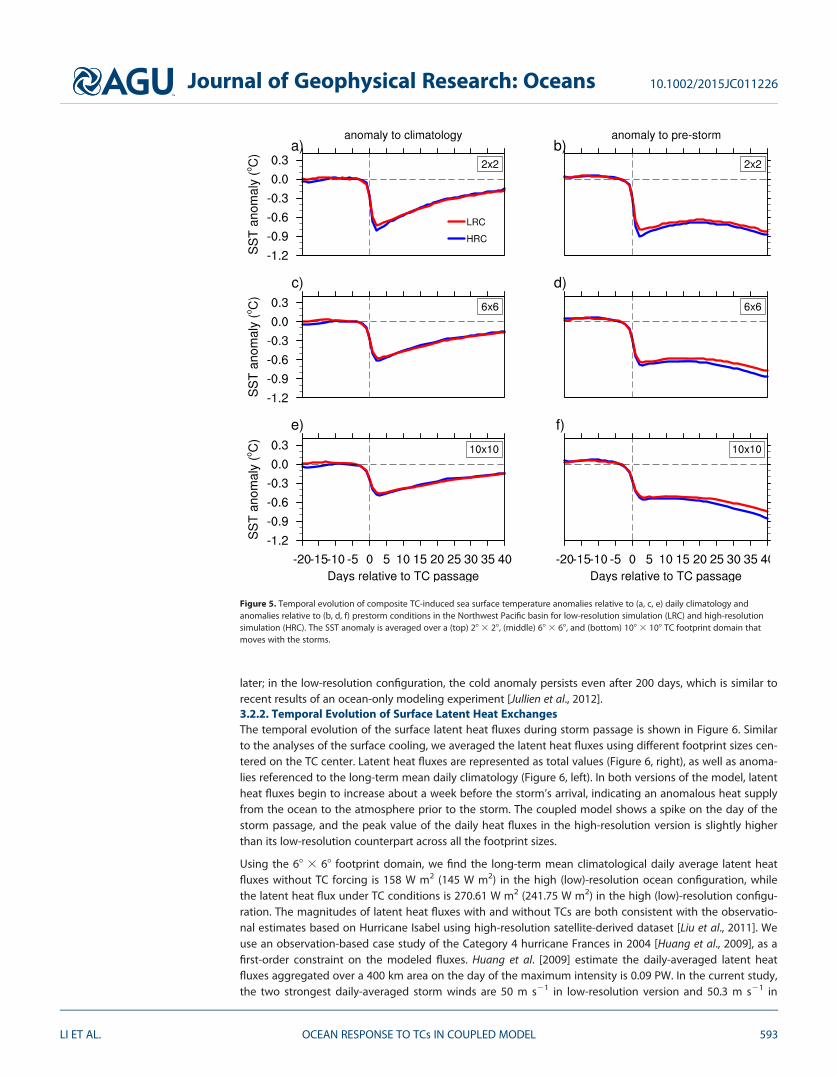
later; in the low-resolution configuration, the cold anomaly persists even after 200 days, which is similar torecent results of an ocean-only modeling experiment [Jullien et al., 2012].3.2.2. Temporal Evolution of Surface Latent Heat ExchangesThe temporal evolution of the surface latent heat fluxes during storm passage is shown in Figure 6. Similarto the analyses of the surface cooling, we averaged the latent heat fluxes using different footprint sizes cen-tered on the TC center. Latent heat fluxes are represented as total values (Figure 6, right), as well as anoma-lies referenced to the long-term mean daily climatology (Figure 6, left). In both versions of the model, latentheat fluxes begin to increase about a week before the storm’s arrival, indicating an anomalous heat supplyfrom the ocean to the atmosphere prior to the storm. The coupled model shows a spike on the day of thestorm passage, and the peak value of the daily heat fluxes in the high-resolution version is slightly higherthan its low-resolution counterpart across all the footprint sizes.

Using the 68 3 68 footprint domain, we find the long-term mean climatological daily average latent heatfluxes without TC forcing is 158 W m2 (145 W m2) in the high (low)-resolution ocean configuration, whilethe latent heat flux under TC conditions is 270.61 W m2 (241.75 W m2) in the high (low)-resolution configu-ration. The magnitudes of latent heat fluxes with and without TCs are both consistent with the observatio-nal estimates based on Hurricane Isabel using high-resolution satellite-derived dataset [Liu et al., 2011]. Weuse an observation-based case study of the Category 4 hurricane Frances in 2004 [Huang et al., 2009], as afirst-order constraint on the modeled fluxes. Huang et al. [2009] estimate the daily-averaged latent heatfluxes aggregated over a 400 km area on the day of the maximum intensity is 0.09 PW. In the current study,the two strongest daily-averaged storm winds are 50 m s21 in low-resolution version and 50.3 m s21 in

Figure 5. Temporal evolution of composite TC-induced sea surface temperature anomalies relative to (a, c, e) daily climatology andanomalies relative to (b, d, f) prestorm conditions in the Northwest Pacific basin for low-resolution simulation (LRC) and high-resolutionsimulation (HRC). The SST anomaly is averaged over a (top) 28 3 28, (middle) 68 3 68, and (bottom) 108 3 108 TC footprint domain thatmoves with the storms.

Journal of Geophysical Research: Oceans 10.1002/2015JC011226

LI ET AL. OCEAN RESPONSE TO TCs IN COUPLED MODEL 593

high-resolution version. Since the daily-averaged wind would underestimate the storm intensity (for reasonsdiscussed in section 3.1), it is possible that instantaneous winds may reach Category 4 (sustained wind>58 m s21). The corresponding latent heat flux peak values integrated over a 400 km area are 0.12 and 0.14PW, which are on the same order with the estimate of Huang et al. [2009].

The model also captures the reduction of latent heat fluxes caused by the cold wake after TC passage. Thefluxes decrease by �30 W m2 when averaged over the 28 area and �20 W m2 when averaged over the 68

area, representing �13–20% decrease compared to the prestorm values. The reduction in latent heat fluxesis consistent with observation-based studies [D’Asaro et al., 2007; Liu et al., 2011], indicating that thecoupled model approaches with a dynamic ocean may be capable of realistically capturing the negativefeedbacks on TC intensification missing from atmosphere-only simulations.3.2.3. Potential Modeled Effects of Mesoscale Ocean Eddies on TC Wake RecoveryHorizontal ocean grid resolution may be important for simulating the storm-scale transient dynamicresponses. In particular, the upper-ocean restratification following TC wakes may be influenced by meso-scale eddy transport and mixing [Haney et al., 2012]. Mesoscale eddies’ horizontal scales are of the order ofthe baroclinic Rossby radius of deformation, typically of O(10 km) [e.g., Killworth, 1997; Chelton et al., 1998].These effects are largely parameterized in the 18 version of the model and explicitly resolved in the 0.18

model.

To explore the effect of mesoscale eddies on the TC-induced upper-ocean response, we analyzed TC activitywithin regions of high and low annual mean eddy kinetic energy (EKE) for both models and satellite-basedobservations [Le Traon et al., 1998]. We estimate EKE using monthly sea surface height anomalies (SSHA) inboth the observational data and model output. The global annual mean EKE for the model simulations andobservations are shown in Figure 7. Both versions of the model generally capture the spatial distribution ofEKE, but the 0.18 model exhibits substantial improvement in the magnitude of EKE compared to the 18

ocean model [see also Maltrud and McClean, 2005; Smith et al., 2000].

Figure 6. Temporal evolution of composite TC-induced surface latent heat fluxes anomalies relative to (a, c, e) daily climatology and their(b, d, f) total values in the Northwest Pacific basin for low-resolution simulation (LRC) and high-resolution simulation (HRC). The latent heatflux anomaly is averaged over a (top) 28 3 28, (middle) 68 3 68, and (bottom) 108 3 108 footprint domain that moves with the storms.

Journal of Geophysical Research: Oceans 10.1002/2015JC011226

LI ET AL. OCEAN RESPONSE TO TCs IN COUPLED MODEL 594

We first examine the potential relationship between wake recovery and background EKE by analyzing aver-age wake responses within a high EKE region (308N–408N, 1308–1758), corresponding to large eddy activitywithin the Kuroshio current and extension. We analyzed the time series composites of the area-averaged(28 3 28) SST anomalies and their e-folding recovery time scales, which is defined as the number of daysnecessary for the SST anomaly to return to e21 of the maximum cooling (Figure 8). The two model versionsexhibit similar characteristics, including the fluctuating pattern of SST time series, the magnitudes of maxi-mum cooling, and the e-folding time scales of 13 days.

We performed further analyses regarding the relationship between EKE, SST cooling and e-folding time byincluding all the storm days globally, in an attempt to gain additional insight into the sensitivity of theresponses to ocean grid resolution. Figure 9 shows the relationship between EKE and e-folding time (upper),and between EKE and maximum SST cooling (lower). EKE is normalized in the right figures, in which the circlesare bin averages and the error bars are their respective standard errors. Results indicate that although the EKEmagnitudes are very different between the model simulations and observations, the TC-induced responsesexhibit similar patterns when using normalized EKE. In particular, the e-folding time in the high EKE regionsare generally consistent between observations and the 0.18 ocean simulation, suggesting the potential impor-tance of eddies in wake recovery and possible improvement of the 0.18 ocean model over the 18 model. How-ever, the relevance and robustness of this result is difficult to interpret given the disparity in the magnitude ofEKE between model simulations and lack of subsurface ocean information from the model output.

Figure 7. Logarithm of the annually averaged eddy kinetic energy (EKE) of (a) satellite-based observations, (b) low-resolution model simu-lation, and (c) high-resolution model simulation.

Journal of Geophysical Research: Oceans 10.1002/2015JC011226

LI ET AL. OCEAN RESPONSE TO TCs IN COUPLED MODEL 595

3.3. First-Order Estimates of TC-Induced Upper-Ocean EnergyBudgetDespite the lack of subsurfaceocean fields, the availability of dailysurface properties and monthlysubsurface ocean temperature ena-bles us to estimate the modeledbasin-scale TC-induced OHC usingdifferent strategies accounting formixing depth (discussed in section2.4). The results are summarized inFigure 10. The average TC mixingdepths and their correspondingOHC estimates are sensitive to thechoice of vertical mixing length-scale calculation; however, themodeled OHC estimates are gener-ally consistent between the twosimulations for each mixing depthcalculation. Differences betweenthe two simulations may be partly

attributed to variations in the background ocean state (supporting information Figure S4), since the upper-ocean temperature structure in the high-resolution model exhibits stronger stratification effects than thelow-resolution model. We find that varying mixing depths based on the climatological vertical ocean tem-perature gradients leads to the largest estimation of TC-induced OHC. This is because the location of themost significant surface cooling corresponds to areas with the deepest mixing, as indicated by the largespread over the mean mixing depth for this method (Figure 10a). In contrast, defining the mixing lengthbased on the depth of the climatological mixed layer yields the smallest TC-induced OHC. This methodlikely underestimates the effect of TCs on the vertical redistribution of ocean heat, even for relatively lowintensity storms considered here, because TC-induced mixing typically penetrates to depths significantlybelow the base of the seasonal mixed layer.

In addition to vertical mixing, TC-induced latent heat fluxes can also contribute to ocean surface cooling.Coupled modeling frameworks have the advantage of capturing surface fluxes within TC regions. We haveshown in section 3.2.2 that both versions of the model are capable of simulating surface latent heatresponses to TCs that are generally consistent with observations. Here we estimate the basin-scale annuallyaccumulated TC-induced latent heat budget within the coupled model and its contribution to the totalupper-ocean heat loss during TC passage.

For each storm day, we integrate the daily average latent heat fluxes from day 0 to day 2 relative to TC pas-sage over a 68 domain. The period of 0–2 days is chosen in order to account for all the latent heat exchangeresponsible for the total upper-ocean heat loss, which we estimate with the maximum SST cooling thatoccurs on day 2 (see Figure 5). The annually accumulated basin-scale latent heat fluxes are 1.70 6 0.16 3

1021 J in the high-resolution model and 1.43 6 0.13 3 1021 J in the low-resolution model, representing 47and 45% of the total TC-induced OHC estimates in the high and low-resolution model configurations,respectively (see also Table 2). This contribution of latent heat exchange is similar to the estimate of Vincentet al. [2012a], who found �43% of ocean heat anomalies are due to latent heat fluxes. Results suggest thatsurface latent heat fluxes account for a substantial amount of heat loss from the upper-ocean during TCevents, which may have important implications for global heat and energy budgets in coupled models.

We apply the basin-scale latent heat flux as a constraint on the oceanic heat convergence induced by TCsin the model simulations (corresponding to F 5 0.53 (0.55) in the high (low)-resolution version in equation(1)). Using the varying mixing depth strategy, we estimate the modeled TC-induced, surface flux-correctedannual Northwestern Pacific basin-scale OHC to be 0.17 3 1022 J in the low-resolution simulation and 0.193 1022 J in the high-resolution simulation, corresponding to a mean annual rate of 0.05 6 0.005 PW (1

Figure 8. Temporal evolution of composite TC-induced sea surface temperatureanomaly relative to daily climatology in the high EKE region (308N–408N, 1308–1758)for high-resolution configuration (HRC) and low-resolution configuration (LRC). Thenumber of storm days and the average e-folding time scales are denoted in theparentheses.

Journal of Geophysical Research: Oceans 10.1002/2015JC011226

LI ET AL. OCEAN RESPONSE TO TCs IN COUPLED MODEL 596

PW 5 1015 W) and 0.06 6 0.005 PW, respectively. In order to make a comparison between the model andobservations, we compare the model results with 60% of the total basin-scale OHC in the observations,since the TC number in the model is about 60% of the observational record in the Northwestern Pacificbasin (see Table 1). Due to the lack of observational estimates of latent heat fluxes within TCs, we applyF 5 0.55 from the model for the observational OHC calculation. The annual surface flux-corrected basin-scale OHC for all the storm intensities in the observations is 0.35 3 1022 J, and 60% of which is 0.21 3 1022

J. This value is comparable with the modeled results. These first-order estimates suggest that the coupledmodel is capable of capturing realistic surface heat fluxes and the upper-ocean heat convergence responsesto tropical cyclones. These preliminary results point to the potential importance of using high-resolutioncoupled modeling approaches to advance our understanding about tropical cyclones and climate.

4. Caveats

This study includes several important simplifying assumptions and caveats, in addition to the methodologi-cal constraints discussed in section 2. Although the 0.58 resolution atmosphere model is shown to be capa-ble of capturing realistic TC circulations and spatial distributions in the Northwestern Pacific, the stormintensities are likely to be underestimated. Thus, potential differences in the storm-induced responses forextremes storms cannot be examined using this model.

Shear instability induced by near-inertial waves contributes to TC-induced SST cooling through turbulententrainment at the base of the mixed layer [Cuypers et al., 2013; Ginis, 2002]. This effect is dependent on themagnitude of near-inertial energy input by the winds to the ocean, as well as the dissipation of the near-inertial energy beneath the oceanic boundary layer. The modeled near-inertial energy input by the winds ishighly dependent on the resolution of the atmospheric component and on the coupling frequency [Jianget al., 2005; Jochum et al., 2013]. The atmospheric model considered here (0.58) is not capable of simulating

Figure 9. Relationship (top) between EKE and e-folding time and (bottom) between EKE and maximum sea surface cooling in observations(green), low-resolution simulation (blue), and high-resolution simulation (red). The circles are bin averages and the error bars are theirrespective standard errors. EKE is normalized on the right figures.

Journal of Geophysical Research: Oceans 10.1002/2015JC011226

LI ET AL. OCEAN RESPONSE TO TCs IN COUPLED MODEL 597

extreme TC events or the fine-scaleatmospheric frontal features thatcan be important for generatingnear-inertial energy input to theocean. Under this situation, the KPPvertical mixing parameterizationscheme used in the model wouldnot provide sufficient near-inertialwave-induced shears [Large et al.,1994; Jochum et al., 2013]. A param-eterization for the dissipation ofnear-inertial energy in the upperocean is not applied in the present(CCSM3.5) or in more recent ver-sions of this model [Jochum et al.,2013]. Improved representation ofthis effect could impact mixed-layerdepth, SST, and precipitation pat-terns [Jochum et al., 2013]. Whetherthe results presented here wouldchange under improved represen-tation of near-inertial waves in themodel is an open question, whichwill be the topic of a future paper.

The effect of mesoscale eddies onocean surface cooling due toentrainment would also likelydepend on the vertical resolution.Both simulations feature the samerelatively coarse vertical resolution(42 levels). Increasing vertical reso-lution (particularly near the surface)may induce a stronger eddy effecton surface cooling that is not cap-tured here.

5. Conclusions

Upper-ocean responses to TCs in a fully coupled Earth system model with varying horizontal ocean gridresolution are investigated in this paper. We analyzed the resolution-dependent responses by examiningsimulated TC climatologies, sea surface cooling responses, and latent heat budgets. We estimate TC-induced OHC in the Northwestern Pacific for both model configurations from near-surface atmosphere and

ocean fields using multiple strat-egies accounting for uncertaintiesin vertical mixing length scales.

Results indicate that the ocean sur-face responses and basin-scaleaggregated TC influences onupper-ocean heat budgets withinthe coupled model configurationsconsidered here are relativelyinsensitive to the choice of oceangrid resolution, when considering

Figure 10. (a) Composite area-mean mixing depth of each storm day in the North-west Pacific basin for low-resolution simulation (LRC) and high-resolution simulation(HRC), computed with three strategies: (left to right) constant mixing depth of 50 m,monthly mean climatological mixed-layer depth, and varying mixing depth derivedfrom ocean potential temperature profiles. The averaging area is a 68 3 68 grid box.The error bars indicate the range of mixing depth within the averaging area for theanalysis period (20 years). (b) Annually accumulated, storm-induced average oceanheat uptake in the Northwest Pacific basin, computed with the three correspondingmixing depth strategies. A discrete method is used to account for the nonuniformmixing within the 68 3 68 averaging domain. Error bars represent the plus or minus 1standard deviation.

Table 2. Surface Latent Heat Flux, Total OHC, Mixing-Induced OHC, and the Stand-ard Deviation of OHC in the Two Model Simulations

Data LRC HRC

Latent heat exchange (J) 1.43e 1 21 1.70e 1 21Total OHC (J) 3.08e 1 21 3.57e 1 21Percentage of latent heat

flux in total OHC45% 47%

Mixing-induced OHC (J) 1.65e 1 21 1.87e 1 21Mixing-induced OHC (PW) 0.05 0.06Standard deviation of the

distribution of annual OHC0.02143 0.03351

Journal of Geophysical Research: Oceans 10.1002/2015JC011226

LI ET AL. OCEAN RESPONSE TO TCs IN COUPLED MODEL 598

18 versus 0.18 resolution. This suggests that the surface eddy flux parameterization in the low-resolutionmodel may be sufficient for capturing the basin-scale horizontal temperature distribution and heat trans-port induced by mesoscale eddies [Danabasoglu et al., 2008]. However, it is important to consider limitationsin the ocean model’s representation of near-inertial wave response when interpreting these results, as wellas relatively coarse (0.58) atmosphere model resolution which is unable to simulate frontal systems impor-tant for near-inertial energy input to the ocean. TC-induced ocean sensitivities to horizontal grid resolutionmay emerge with improved representation of near-inertial waves, which could influence transient intrasea-sonal dynamic responses to TC forcing as well as poststorm wake recovery, ocean heat uptake, upper-oceancurrents, and meridional transports.

Given the magnitude of the modeled and observed TC-induced fluxes of heat and momentum at theatmosphere-ocean interface, and the resulting positive ocean heat convergence, these results point to theimportance of coupled model approaches to developing a more complete understanding about the rela-tionship between TCs and climate. Coupled modeling initiatives utilizing ultra-high-resolution modelingframeworks may provide fundamental insight to potential TC-induced feedbacks that influence large-scaleocean and atmosphere heat budgets and circulation patterns.

ReferencesBacmeister, J. T., M. F. Wehner, R. B. Neale, A. Gettelman, C. Hannay, P. H. Lauritzen, J. M. Caron, and J. E. Truesdale (2013), Exploratory high-

resolution climate simulations using the community atmosphere model (CAM), J. Clim., 27(9), 3073–3099, doi:10.1175/JCLI-D-13-00387.1.Bell, R., J. Strachan, P. L. Vidale, K. Hodges, and M. Roberts (2013), Response of tropical cyclones to idealized climate change experiments in

a global high-resolution coupled general circulation model, J. Clim., 26(20), 7966–7980, doi:10.1175/JCLI-D-12-00749.1.Bender, M. A., and I. Ginis (2000), Real-case simulations of hurricane-ocean interaction using a high-resolution coupled model: Effects on

hurricane intensity, Mon. Weather Rev., 128(4), 917–946.Boos, W. R., J. R. Scott, and K. A. Emanuel (2004), Transient diapycnal mixing and the meridional overturning circulation, J. Phys. Oceanogr.,

34(1), 334–341, doi:10.1175/1520-0485(2004)034< 0334:TDMATM>2.0.CO;2.Bueti, M. R., I. Ginis, L. M. Rothstein, and S. M. Griffies (2014), Tropical cyclone-induced thermocline warming and its regional and global

impacts, J. Clim., 27, 6978–6999, doi:10.1175/JCLI-D-14-00152.1.Camargo, S. J. (2013), Global and regional aspects of tropical cyclone activity in the CMIP5 models, J. Clim., 26(24), 9880–9902, doi:10.1175/

JCLI-D-12-00549.1.Camargo, S. J., and S. E. Zebiak (2002), Improving the detection and tracking of tropical cyclones in atmospheric general circulation mod-

els, Weather Forecasting, 17(6), 1152–1162.Camargo, S. J., A. G. Barnston, and S. E. Zebiak (2005), A statistical assessment of tropical cyclone activity in atmospheric general circulation

models, Tellus, Ser. A, 57(4), 589–604, doi:10.3402/tellusa.v57i4.14705.Chelton, D. B., R. A. deSzoeke, M. G. Schlax, K. E. I. Naggar, N. Siwertz (1998), Geographical variability of the first baroclinic Rossby radius of

deformation, J. Phys. Oceanogr., 28, 433–460.Cheng, L., J. Zhu, and R. L. Sriver (2014), Global representation of tropical cyclone-induced ocean thermal changes using Argo data—Part

1: Methods and results, Ocean Sci. Discuss., 11(6), 2831–2878, doi:10.5194/osd-11-2831-2014.Cuypers, Y., X. Le Vaillant, P. Bouruet-Aubertot, J. Vialard, and M. J. McPhaden (2013), Tropical storm-induced near-inertial internal waves

during the Cirene experiment: Energy fluxes and impact on vertical mixing, J. Geophys. Res. Oceans, 118, 358–380, doi:10.1029/2012JC007881.

Danabasoglu, G., R. Ferrari, and J. C. McWilliams (2008), Sensitivity of an Ocean General Circulation Model to a Parameterization of Near-Surface Eddy Fluxes, J. Clim., 21(6), 1192–1208, doi:10.1175/2007JCLI1508.1.

Danabasoglu, G., S. C. Bates, B. P. Briegleb, S. R. Jayne, M. Jochum, W. G. Large, S. Peacock, and S. G. Yeager (2012), The CCSM4 ocean com-ponent, J. Clim., 25(5), 1361–1389, doi:10.1175/JCLI-D-11-00091.1.

Dare, R. A., and J. L. McBride (2011), Sea surface temperature response to tropical cyclones, Mon. Weather Rev., 139(12), 3798–3808, doi:10.1175/MWR-D-10-05019.1.

D’Asaro, E. A., T. B. Sanford, P. P. Niiler, and E. J. Terrill (2007), Cold wake of Hurricane Frances, Geophys. Res. Lett., 34, L15609, doi:10.1029/2007GL030160.

Emanuel, K. (2001), Contribution of tropical cyclones to meridional heat transport by the oceans, J. Geophys. Res., 106(D14), 14,771–14,781,doi:10.1029/2000JD900641.

Gent, P. R., S. G. Yeager, R. B. Neale, S. Levis, and D. A. Bailey (2010), Improvements in a half degree atmosphere/land version of the CCSM,Clim. Dyn., 34(6), 819–833, doi:10.1007/s00382-009-0614-8.

Gentemann, C. L., T. Meissner, and F. J. Wentz (2010), Accuracy of satellite sea surface temperatures at 7 and 11 GHz, IEEE Trans. Geosci.Remote Sens., 48(3), 1009–1018, doi:10.1109/TGRS.2009.2030322.

Ginis, I. (2002), Tropical cyclone-ocean interactions, Adv. Fluid Mech., 33, 83–114.Gualdi, S., E. Scoccimarro, and A. Navarra (2008), Changes in tropical cyclone activity due to global warming: Results from a high-resolution

coupled general circulation model, J. Clim., 21(20), 5204–5228, doi:10.1175/2008JCLI1921.1.Haney, S., S. Bachman, B. Cooper, S. Kupper, K. McCaffrey, L. Van Roekel, S. Stevenson, B. Fox-Kemper, and R. Ferrari (2012), Hurricane wake

restratification rates of one-, two-and three-dimensional processes, J. Mar. Res., 70(6), 824–850.Hart, R. E. (2011), An inverse relationship between aggregate northern hemisphere tropical cyclone activity and subsequent winter climate,

Geophys. Res. Lett., 38, L01705, doi:10.1029/2010GL045612.Hu, A., and G. A. Meehl (2009), Effect of the Atlantic hurricanes on the oceanic meridional overturning circulation and heat transport, Geo-

phys. Res. Lett., 36, L03702, doi:10.1029/2008GL036680.Huang, P., T. B. Sanford, and J. Imberger (2009), Heat and turbulent kinetic energy budgets for surface layer cooling induced by the pas-

sage of Hurricane Frances (2004), J. Geophys. Res., 114, C12023, doi:10.1029/2009JC005603.

AcknowledgmentsWe thank Ben Kirtman for providingthe model output for the analyses inthis study. Marlos Goes was partlysupported by NOAA/AOML and theNOAA Climate Program Office. We alsothank Kerry Emanuel for providingglobal TC best track data: http://eaps4.mit.edu/faculty/Emanuel/products. TheOI SST product is from the RemoteSensing System website (http://www.remss.com/) and is sponsored byNational Oceanographic PartnershipProgram (NOPP), the NASA EarthScience Physical OceanographyProgram, and the NASA MEaSUREsDISCOVER Project. The ORAS4 oceanreanalysis data are provided by theAsia-Pacific Data-Research Center ofthe International Pacific ResearchCenter, which can be found on theirwebsite at http://apdrc.soest.hawaii.edu/data/data.php. The WOA13product is provided by NOAA NationalOceanographic Data Center. The windshear climatology is from NCEPReanalysis, which is provided by theNOAA/OAR/ESRL PSD, Boulder,Colorado, USA, from their website athttp://www.esrl.noaa.gov/psd/. Thealtimeter products were produced bySsalto/Duacs and distributed by Avisowith support from Cnes.

Journal of Geophysical Research: Oceans 10.1002/2015JC011226

LI ET AL. OCEAN RESPONSE TO TCs IN COUPLED MODEL 599

Jansen, M., and R. Ferrari (2009), Impact of the latitudinal distribution of tropical cyclones on ocean heat transport, Geophys. Res. Lett., 36,L06604, doi:10.1029/2008GL036796.

Jansen, M. F., R. Ferrari, and T. A. Mooring (2010), Seasonal versus permanent thermocline warming by tropical cyclones, Geophys. Res. Lett.,37, L03602, doi:10.1029/2009GL041808.

Jiang, J., Y. Liu, and W. Perrie (2005), Estimating the energy flux from the wind to ocean inertial motions: The sensitivity to surface windfields, Geophys. Res. Lett., 32, L15610–2844, doi:10.1029/2005GL023289.

Jochum, M., B. P. Briegleb, G. Danabasoglu, W. G. Large, N. J. Norton, S. R. Jayne, M. H. Alford, and F. O. Bryan (2013), The Impact of OceanicNear-Inertial Waves on Climate, J. Clim., 26(9), 2883–2844, doi:10.1175/JCLI-D-12-00181.1.

Jullien, S., C. E. Menkes, P. Marchesiello, N. C. Jourdain, M. Lengaigne, A. Koch-Larrouy, J. Lefevre, E. M. Vincent, and V. Faure (2012),Impact of tropical cyclones on the heat budget of the South Pacific Ocean, J. Phys. Oceanogr., 42(11), 1882–1906, doi:10.1175/JPO-D-11-0133.1.

Jullien, S., P. Marchesiello, C. E. Menkes, J. Lefevre, N. C. Jourdain, G. Samson, and M. Lengaigne (2014), Ocean feedback to tropical cyclo-nes: Climatology and processes, Clim. Dyn., 43, 2831–2854, doi:10.1007/s00382-014-2096-6.

Killworth, P. D. (1997), On the parameterization of eddy transfer, part I: Theory, J. Mar. Res., 55, 1171–1197, doi:10.1357/0022240973224102.Kim, H.-S., G. A. Vecchi, T. R. Knutson, W. G. Anderson, T. L. Delworth, A. Rosati, F. Zeng, and M. Zhao (2014), Tropical cyclone simulation and

response to CO2 doubling in the GFDL CM2.5 high-resolution coupled climate model, J. Clim., 27, 8034–8054, doi:10.1175/JCLI-D-13-00475.1.Kirtman, B. P., et al. (2012), Impact of ocean model resolution on CCSM climate simulations, Clim. Dyn., 39(6), 1303–1328, doi:10.1007/

s00382-012-1500-3.Large, W. G., J. C. McWilliams, and S. C. Doney (1994), Oceanic vertical mixing: A review and a model with a nonlocal boundary layer

parameterization, Rev. Geophys., 32, 363–403.Locarnini, R. A., et al. (2013), World Ocean Atlas 2013, Volume 1: Temperature, S. Levitus, Ed., A. Mishonov Technical Ed., NOAA Atlas NESDIS

73, 40 pp.Le Traon, P. Y., F. Nadal, and N. Ducet (1998), An improved mapping method of multisatellite altimeter data, J. Atmos. Oceanic Technol.,

15(2), 522–534.Li, F., W. D. Collins, M. F. Wehner, and L. R. Leung (2013), Hurricanes in an aquaplanet world: Implications of the impacts of external forcing

and model horizontal resolution, J. Adv. Model. Earth Syst., 5, 134–145, doi:10.1002/jame.20020.Liu, J., J. A. Curry, C. A. Clayson, and M. A. Bourassa (2011), High-resolution satellite surface latent heat fluxes in North Atlantic Hurricanes,

Mon. Weather Rev., 139(9), 2735–2747, doi:10.1175/2011MWR3548.1.Lloyd, I. D., and G. A. Vecchi (2011), Observational evidence for oceanic controls on hurricane intensity, J. Clim., 24(4), 1138–1153, doi:

10.1175/2010JCLI3763.1.Maltrud, M. E., and J. L. McClean (2005), An eddy resolving global 1/108 ocean simulation, Ocean Modell., 8(1–2), 31–54, doi:10.1016/

j.ocemod.2003.12.001.Manganello, J. V., et al. (2012), Tropical cyclone climatology in a 10-km global atmospheric GCM: Toward weather-resolving climate model-

ing, J. Clim., 25(11), 3867–3893, doi:10.1175/JCLI-D-11-00346.1.Manucharyan, G. E., C. M. Brierley, and A. V. Fedorov (2011), Climate impacts of intermittent upper ocean mixing induced by tropical cyclo-

nes, J. Geophys. Res. Oceans, 116(C11), C11038–30, doi:10.1029/2011JC007295.McClean, J. L., et al. (2011), A prototype two-decade fully-coupled fine-resolution CCSM simulation, Ocean Modell., 39(1–2), 10–30, doi:

10.1016/j.ocemod.2011.02.011.Mei, W., and C. Pasquero (2012), Spatial and temporal characterization of sea surface temperature response to tropical cyclones, J. Clim.,

26(11), 3745–3765, doi:10.1175/JCLI-D-12-00125.1.Mei, W., F. Primeau, J. C. McWilliams, and C. Pasquero (2013), Sea surface height evidence for long-term warming effects of tropical cyclo-

nes on the ocean, Proc. Natl. Acad. Sci. U. S. A., 110, 15,207–15,210, doi:10.1073/pnas.1306753110.Murakami, H., and M. Sugi (2010), Effect of model resolution on tropical cyclone climate projections, SOLA, 6, 73–76, doi:10.2151/sola.2010-019.Park, J. J., Y.-O. Kwon, and J. F. Price (2011), Argo array observation of ocean heat content changes induced by tropical cyclones in the

north Pacific, J. Geophys. Res., 116, C12025, doi:10.1029/2011JC007165.Pasquero, C., and K. Emanuel (2008), Tropical cyclones and transient upper-ocean warming, J. Clim., 21(1), 149–162, doi:10.1175/

2007JCLI1550.1.Rathmann, N. M., S. Yang, and E. Kaas (2014), Tropical cyclones in enhanced resolution CMIP5 experiments, Clim. Dyn., 42(3–4), 665–681,

doi:10.1007/s00382-013-1818-5.Scoccimarro, E., S. Gualdi, A. Bellucci, A. Sanna, P. Giuseppe Fogli, E. Manzini, M. Vichi, P. Oddo, and A. Navarra (2011), Effects of tropical

cyclones on ocean heat transport in a high-resolution coupled general circulation model, J. Clim., 24(16), 4368–4384, doi:10.1175/2011JCLI4104.1.

Shaevitz, D. A., et al. (2014), Characteristics of tropical cyclones in high-resolution models in the present climate, J. Adv. Model. Earth Syst.,6, 1154–1172, doi:10.1002/2014MS000372.

Small, R. J., et al. (2014), A new synoptic scale resolving global climate simulation using the Community Earth System Model, J. Adv. Model.Earth Syst., 6, 1065–1094, doi:10.1002/2014MS000363.

Smith, R. D., M. E. Maltrud, F. O. Bryan, and M. W. Hecht (2000), Numerical simulation of the North Atlantic Ocean at 1/108, J. Phys. Ocean-ogr., 30(7), 1532–1561, doi:10.1175/1520-0485(2000)030<1532:NSOTNA>2.0.CO;2.

Sriver, R. L. (2013), Observational evidence supports the role of tropical cyclones in regulating climate, Proc. Natl. Acad. Sci. U. S. A., 110(38),15,173–15,174, doi:10.1073/pnas.1314721110.

Sriver, R. L., and M. Huber (2007), Observational evidence for an ocean heat pump induced by tropical cyclones, Nature, 447(7144), 577–580, doi:10.1038/nature05785.

Sriver, R. L., and M. Huber (2010), Modeled sensitivity of upper thermocline properties to tropical cyclone winds and possible feedbacks onthe Hadley circulation, Geophys. Res. Lett., 37, L08704, doi:10.1029/2010GL042836.

Sriver, R. L., M. Huber, and J. Nusbaumer (2008), Investigating tropical cyclone-climate feedbacks using the TRMM Microwave Imager andthe Quick Scatterometer, Geochem. Geophys. Geosyst., 9, Q09V11, doi:10.1029/2007GC001842.

Sriver, R. L., M. Goes, M. E. Mann, and K. Keller (2010), Climate response to tropical cyclone-induced ocean mixing in an Earth system modelof intermediate complexity, J. Geophys. Res., 115, C10042, doi:10.1029/2010JC006106.

Strachan, J., P. L. Vidale, K. Hodges, M. Roberts, and M.-E. Demory (2012), Investigating global tropical cyclone activity with a Hierarchy ofAGCMs: The role of model resolution, J. Clim., 26(1), 133–152, doi:10.1175/JCLI-D-12-00012.1.

Vincent, E. M., M. Lengaigne, J. Vialard, G. Madec, N. C. Jourdain, and S. Masson (2012a), Assessing the oceanic control on the amplitude ofsea surface cooling induced by tropical cyclones, J. Geophys. Res., 117(C5), doi:10.1029/2011JC007705.

Journal of Geophysical Research: Oceans 10.1002/2015JC011226

LI ET AL. OCEAN RESPONSE TO TCs IN COUPLED MODEL 600

Vincent, E. M., M. Lengaigne, G. Madec, J. Vialard, G. Samson, N. C. Jourdain, C. E. Menkes, and S. Jullien (2012b), Processes setting the char-acteristics of sea surface cooling induced by tropical cyclones, J. Geophys. Res., 117(C2), doi:10.1029/2011JC007396.

Vincent, E. M., G. Madec, M. Lengaigne, J. Vialard, and A. Koch-Larrouy (2013), Influence of tropical cyclones on sea surface temperatureseasonal cycle and ocean heat transport, Clim. Dyn., 41(7–8), 2019–2038, doi:10.1007/s00382-012-1556-0.

Walsh, K., S. Lavender, E. Scoccimarro, and H. Murakami (2013), Resolution dependence of tropical cyclone formation in CMIP3 and finerresolution models, Clim. Dyn., 40(3–4), 585–599, doi:10.1007/s00382-012-1298-z.

Wang, X., C. Wang, G. Han, W. Li, and X. Wu (2014), Effects of tropical cyclones on large-scale circulation and ocean heat transport in theSouth China Sea, Clim. Dyn., 43, 3351–3366, doi:10.1007/s00382-014-2109-5.

Wehner, M. F., G. Bala, P. Duffy, A. A. Mirin, and R. Romano (2010), Towards direct simulation of future tropical cyclone statistics in a high-resolution global atmospheric model, Adv. Meteorol., 2010, 915303, doi:10.1155/2010/915303.

Wehner, M. F., et al. (2014), The effect of horizontal resolution on simulation quality in the community atmospheric model, CAM5.1, J. Adv.Model. Earth Syst., 6, 980–997, doi:10.1002/2013MS000276.

Zhao, M., I. M. Held, S.-J. Lin, and G. A. Vecchi (2009), Simulations of global hurricane climatology, interannual variability, and response toglobal warming using a 50-km resolution GCM, J. Clim., 22(24), 6653–6678, doi:10.1175/2009JCLI3049.1.

Journal of Geophysical Research: Oceans 10.1002/2015JC011226

LI ET AL. OCEAN RESPONSE TO TCs IN COUPLED MODEL 601