Information and Computation 234 (2014) 26–43

Contents lists available at ScienceDirect

Information and Computation

www.elsevier.com/locate/yinco

Modeling, analyzing and slicing periodic distributedcomputations ✩

Vijay K. Garg ∗, Anurag Agarwal 1, Vinit Ogale 2

The University of Texas at Austin, Austin, TX 78712-1084, USA

a r t i c l e i n f o a b s t r a c t

Article history:Available online 14 December 2013

Keywords:Predicate detectionLiveness violationd-DiagramRecurrent computation

The earlier work on predicate detection has assumed that the given computation is finite.Detecting violation of a liveness predicate requires that the predicate be evaluated onan infinite computation. In this work, we develop the theory and associated algorithmsfor predicate detection in infinite runs. In practice, an infinite run can be determined infinite time if it consists of a recurrent behavior with some finite prefix. Therefore, ourstudy is restricted to such runs. We introduce the concept of d-diagram, which is a finiterepresentation of infinite directed graphs. Given a d-diagram that represents an infinitedistributed computation, we solve the problem of determining if a global predicate everbecame true in the computation. The crucial aspect of this problem is the stopping rulethat tells us when to conclude that the predicate can never become true in future. Wealso provide an algorithm to provide vector timestamps to events in the computationfor determining the dependency relationship between any two events in the infinite run.Finally, we give an algorithm to compute a slice of a d-diagram which concisely capturesall the consistent global states of the computation satisfying the given predicate.

© 2013 Elsevier Inc. All rights reserved.

1. Introduction

Correctness properties of distributed programs can be classified either as safety properties or liveness properties. Infor-mally, a safety property states that the program never enters a bad (or an unsafe) state, and a liveness property states thatthe program eventually enters into a good state. For example, in the classical dining philosopher problem a safety propertyis that “two neighboring philosophers never eat concurrently” and a liveness property is that “every hungry philosophereventually eats.” Assume that a programmer is interested in monitoring for violation of a correctness property in her dis-tributed program. It is clear how a runtime monitoring system would check for violation of a safety property. If it detectsthat there exists a consistent global state [1] in which two neighboring philosophers are eating then the safety property isviolated. The literature in the area of global predicate detection deals with the complexity and algorithms for such tasks[2,3]. However, the problem of detecting violation of the liveness property is harder. At first it appears that detecting viola-tion of a liveness property may even be impossible. After all, a liveness property requires something to be true eventuallyand therefore no finite observation can detect the violation. We show in this paper a technique that can be used to infer

✩ Part of the work was performed at the University of Texas at Austin supported in part by the NSF Grants CNS-0718990, CNS-1115808, Texas EducationBoard Grant 781, SRC Grant 2006-TJ-1426, and Cullen Trust for Higher Education Endowed Professorship.

* Corresponding author.E-mail address: garg@ece.utexas.edu (V.K. Garg).

1 Currently at Google.2 Currently at Microsoft.

0890-5401/$ – see front matter © 2013 Elsevier Inc. All rights reserved.http://dx.doi.org/10.1016/j.ic.2013.11.002

V.K. Garg et al. / Information and Computation 234 (2014) 26–43 27

Fig. 1. A finite distributed computation C of dining philosophers.

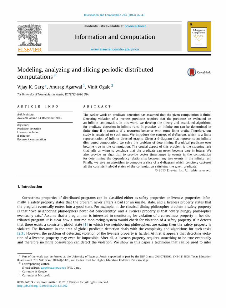
Fig. 2. (a) A d-diagram and (b) its corresponding infinite poset.

violation of a liveness property in spite of finite observations. Such a technique would be a basic requirement for detectinga temporal logic formula [4] on a computation for runtime verification.

There are three important components in our technique. First, we use the notion of a recurrent global state. Informally,a global state is recurrent in a computation γ if it occurs more than once in it. Existence of a recurrent global state impliesthat there exists an infinite computation δ in which the set of events between two occurrences of can be repeated adinfinitum. Note that γ may not even be a prefix of δ. The actual behavior of the program may not follow the execution of δ

due to nondeterminism. However, we know that δ is a legal behavior of the program and therefore violation of the livenessproperty in δ shows a bug in the program. We note here that in this paper we are only interested in algorithms that donot use randomization to ensure liveness properties. For a randomized algorithm, existence of δ may be okay because thealgorithm may guarantee liveness only with probability one.

For example, in Fig. 1, a global state repeats where the same philosopher P1 is hungry and has not eaten in betweenthese occurrences. P1 does get to eat after the second occurrence of the recurrent global state; and, therefore a check that“every hungry philosopher gets to eat” does not reveal the bug. It is simple to construct an infinite computation δ from theobserved finite computation γ in which P1 never eats. We simply repeat the execution between the first and the secondinstance of the recurrent global state. This example shows that the approach of capturing a periodic part of a computationcan result in detection of bugs that may have gone undetected if the periodic behavior is not considered.

The second component of our technique is to develop a finite representation of the infinite behavior γ . Mathematically,we need a finite representation of the infinite but periodic poset γ . In this paper, we propose the notion of d-diagram tocapture infinite periodic posets. Just as finite directed acyclic graphs (dag’s) have been used to represent and analyze finitecomputations, d-diagrams may be used for representing periodic infinite distributed computations for monitoring or loggingpurposes. The logging may be useful for replay or offline analysis of the computation. Fig. 2 shows a d-diagram and thecorresponding infinite computation. The formal semantics of a d-diagram is given in Section 4. Intuitively, the infinite posetcorresponds to the infinite unrolling of the recurrent part of the d-diagram.

The third component of our technique is to develop efficient algorithms for analyzing the infinite poset given as ad-diagram. Three kinds of computation analysis have been used in past for finite computations. The first analysis is basedon vector clocks which allows one to answer if two events are dependent or concurrent, for example, works by Fidge [5]and Mattern [6]. We extend the algorithm for timestamping events of a finite poset to that for the infinite poset. Of course,since the set of events is infinite, we do not give explicit timestamp for all events, but only an implicit method that allowsefficient calculation of dependency information between any two events when desired. The second analysis we use is todetect a global predicate B on the infinite poset given as a d-diagram. In other words, we are interested in determining ifthere exists a consistent global state which satisfies B . Since the computation is infinite, we cannot employ the traditionalalgorithms [2,3] for predicate detection. Because the behavior is periodic it is natural that a finite prefix of the infinite posetmay be sufficient to analyze. The crucial problem is to determine the number of times the recurrent part of the d-diagrammust be unrolled so that we can guarantee that B is true in the finite prefix iff it is true in the infinite computation. Weshow in this paper that it is sufficient to unroll the d-diagram N times where N is the number of processes in the system.The third analysis is based on the notion of slicing a computation introduced in [7,8]. Informally, a computation slice (orsimply a slice) is a concise representation of all those consistent cuts of the computation that satisfy the predicate. Slicing

28 V.K. Garg et al. / Information and Computation 234 (2014) 26–43

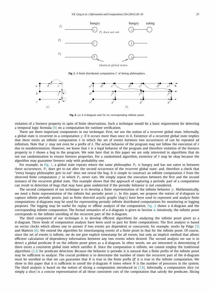
Fig. 3. A (faulty) distributed mutual exclusion algorithm with FIFO channels.

is crucial in detecting nested temporal logic predicates of a distributed computation in the partial order model. Sen andGarg use slicing in [23] to detect a subset of CTL called Regular CTL. Ogale and Garg use it to detect another temporal logiccalled BTL. All the earlier work on computing slices was based on finite computation and we extend that work for infinitecomputations in this paper. For example, the interpretation of “a hungry philosopher never gets to eat” was modified byearlier work to “a hungry philosopher does not eat by the end of the computation.” This interpretation, although usefulin some cases, is not accurate and may give false positives when employed by the programmer to detect bugs. This paperis the first one to explicitly analyze the periodic behavior to ensure that the interpretation of formulas is on the infinitecomputation.

In summary, this paper makes the following contributions:

• We introduce the notion of recurrent global states in a distributed computation and propose a method to detect them.• We introduce and study a finite representation of infinite directed computations called d-diagrams.• We provide a method of timestamping nodes of a d-diagram so that the happened-before relation can be efficiently

determined between any two events in the given infinite computation.• We define the notion of core of a d-diagram that allows us to use any predicate detection algorithm for finite compu-

tations on infinite computations as well.• We present an algorithm to compute slice of the periodic computation represented using a d-diagram.

2. A motivating example: a mutual exclusion algorithm

In this section we give a motivating example for the theory proposed in the paper. Consider the distributed algorithm(shown in Fig. 3) proposed by a programmer to coordinate access to the critical section by processes P1 . . . P N in a dis-tributed system. In this algorithm, a process can enter the critical section only if it has the token. If a process is hungryand it does not have the token, it sends a request to all processes. Every process Pk maintains an array reqF lag whichkeeps track of all processes that have outstanding requests for the token. When a process with the token is done with itscritical section, it sends the token to any process that has an outstanding request. It also sends a release message to all otherprocesses so that they can reset the corresponding reqF lag .

V.K. Garg et al. / Information and Computation 234 (2014) 26–43 29

Fig. 4. A finite distributed computation α for the mutex algorithm.

Fig. 5. A p-diagram derived from α that shows violation of a liveness property.

Now suppose that the programmer is interested in testing this algorithm. When she runs the algorithm, suppose thatthe following execution α takes place. All three philosophers get hungry. P1 eats first and then sends token to P2 who eatsnext. P1 gets hungry again and gets the token from P2. Once P1 has finished eating, it sends the token to P3 who eats last.

The distributed computation, α can be described in more detail by the following sequences of events at each process.

P1: reqCS, recvReq from P3, eats, recvReq from P2, relCS sending token to P2, reqCS, recvToken from P2, eats, relCS sendingtoken to P3P2: recvReq from P3, reqCS, recvToken from P1, recvReq from P1, relCS sending token to P1, recvRel from P1P3: reqCS, recvReq from P2, recvRel from P1, recvReq from P1, recvRel from P2, recvToken from P1, eat

The distributed computation α shown in Fig. 4 satisfies the standard safety and liveness properties: two processes do noteat at the same time and every hungry process eventually eats. However, with the techniques proposed in the paper wewould be able to construct an infinite computation α′ that is a valid execution and violates the liveness property.

Consider the following prefix β of computation α:

P1: reqCS, recvReq from P3, eatsP2: recvReq from P3P3: reqCS

The global state after β is:State of P1: haveToken = true; reqFlag = (false, false, true); state = thinkingState of P2: haveToken = false; reqFlag = (false, false, true); state = thinkingState of P3: haveToken = false; reqFlag = (false, false, true); state = thinking

Note that the same global state occurs in α after P1 has eaten twice in the following prefix: (β followed by γ )

P1: reqCS, recvReq from P3, eats, recvReq from P2, relCS sending token to P2, reqCS, recvToken from P2, eatsP2: recvReq from P3, reqCS, recvToken from P1, recvReq from P1, relCS sending token to P1P3: reqCS, recvReq from P2, recvRel from P1, recvReq from P1, recvRel from P2

Since the global state is identical after executing β and β followed by γ , there exists a valid execution α′ in which β isfollowed by γ an infinite number of times. The execution α′ violates the liveness property because P3 stays hungry forever.The infinite execution derived from α is shown as a p-diagram in Fig. 5.

Remark. The algorithm can be fixed by making two changes. First, we should maintain a queue of requests at all processesrather than a set of requests as implemented in Fig. 3 by the boolean array reqF lag . Second, a process with the token thathas eaten last must release the token if the queue of requesting processes is nonempty.

30 V.K. Garg et al. / Information and Computation 234 (2014) 26–43

3. Model of a distributed computation

We first describe our model of a distributed computation. We assume a message passing asynchronous system with-out any shared memory or a global clock. A distributed program consists of N sequential processes denoted by P ={P1, P2, . . . , P N} communicating via asynchronous messages. A local computation of a process is a sequence of events. Anevent is either an internal event, a send event or a receive event. When an event is executed, it changes the state of theprocess (and possibly the state of incoming or outgoing channels). The predecessor and successor events of e on the processon which e occurs are denoted by pred(e) and succ(e).

Generally a distributed computation is modeled as a partial order of a set of events, called the happened-before rela-tion [9]. In this paper, we instead use directed graphs to model distributed computations as done in [8]. When the graph isacyclic, it represents a distributed computation. When the distributed computation is infinite, the directed graph that mod-els the computation is also infinite. An infinite distributed computation is periodic if it consists of a subcomputation thatis repeated forever. Directed graphs allow us to represent both the computation and its slice with respect to a predicate ina uniform fashion. However, as opposed to the earlier work, our computations can be infinite and as a result, the directedgraphs used to model the computation can be infinite.

Given a directed graph G = 〈E,→〉, we define a consistent cut as a set of vertices such that if the subset contains avertex then it contains all its incoming neighbors. For example, the set C = {a1,b1, c1,d1, e1, f 1, g1} is a consistent cut forthe graph shown in Fig. 8(b). The set {a1,b1, c1,d1, e1, g1} is not consistent because it includes g1, but does not include itsincoming neighbor f 1. The set of finite consistent cuts for graph G is denoted by C(G).

In this work we focus only on finite consistent cuts (or finite order ideals [10]) as they are the ones of interest fordistributed computing.

A frontier of a consistent cut is the set of those events of the cut whose successors, if they exist, are not contained inthe cut. Formally,

frontier(C) = {x ∈ C

∣∣ succ(x) exists ⇒ succ(x) /∈ C}

For the cut C in Fig. 8(b), frontier(C) = {e1, f 1, g1}. A consistent cut is uniquely characterized by its frontier and in thispaper we always identify a consistent cut by its frontier.

Two events are said to be consistent iff they are contained in the frontier of some consistent cut, otherwise they areinconsistent. It can be verified that events e and f are consistent iff there is no path in the computation from succ(e) to fand from succ( f ) to e.

4. Infinite directed graphs

From distributed computing perspective, our intention is to provide a model for an infinite computation of a distributedsystem which eventually becomes periodic. Although a distributed computation in the happened-before model [9] is alwaysrepresented using a poset, it is useful to have a model of infinite directed graphs for the purpose of slicing [7,8]. Thedirected graph does not capture the order between events in the computation but it is used to capture the set of possibleconsistent cuts or global states of the system. To this end, we introduce the notion of d-diagram (directed graph diagram).

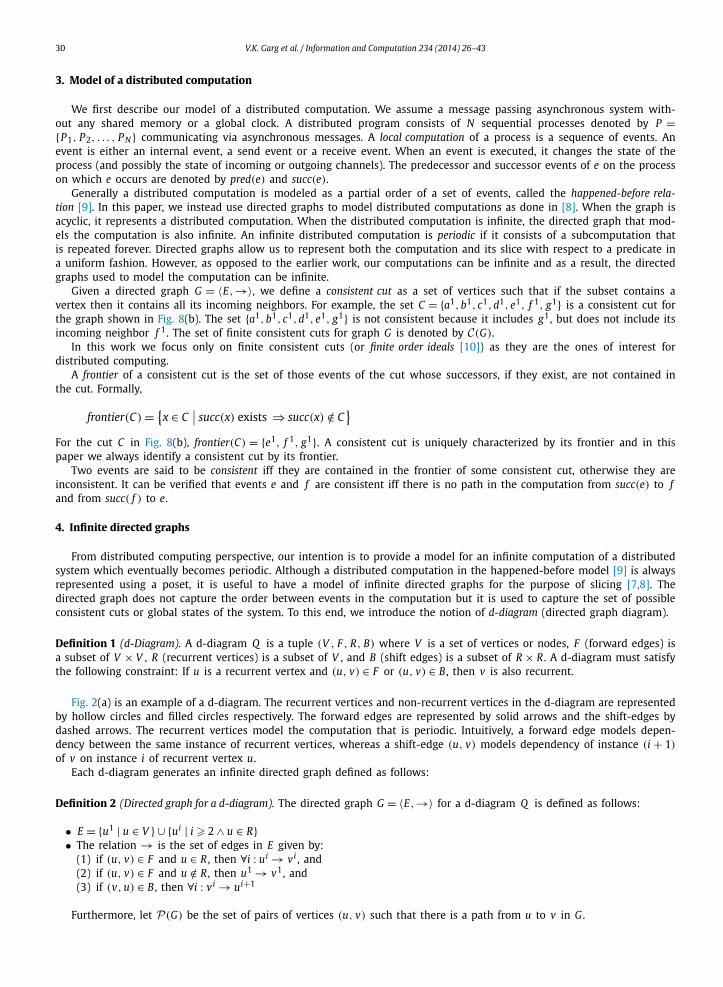
Definition 1 (d-Diagram). A d-diagram Q is a tuple (V , F , R, B) where V is a set of vertices or nodes, F (forward edges) isa subset of V × V , R (recurrent vertices) is a subset of V , and B (shift edges) is a subset of R × R . A d-diagram must satisfythe following constraint: If u is a recurrent vertex and (u, v) ∈ F or (u, v) ∈ B , then v is also recurrent.

Fig. 2(a) is an example of a d-diagram. The recurrent vertices and non-recurrent vertices in the d-diagram are representedby hollow circles and filled circles respectively. The forward edges are represented by solid arrows and the shift-edges bydashed arrows. The recurrent vertices model the computation that is periodic. Intuitively, a forward edge models depen-dency between the same instance of recurrent vertices, whereas a shift-edge (u, v) models dependency of instance (i + 1)

of v on instance i of recurrent vertex u.Each d-diagram generates an infinite directed graph defined as follows:

Definition 2 (Directed graph for a d-diagram). The directed graph G = 〈E,→〉 for a d-diagram Q is defined as follows:

• E = {u1 | u ∈ V } ∪ {ui | i � 2 ∧ u ∈ R}• The relation → is the set of edges in E given by:

(1) if (u, v) ∈ F and u ∈ R , then ∀i : ui → vi , and(2) if (u, v) ∈ F and u /∈ R , then u1 → v1, and(3) if (v, u) ∈ B , then ∀i : vi → ui+1

Furthermore, let P(G) be the set of pairs of vertices (u, v) such that there is a path from u to v in G .

V.K. Garg et al. / Information and Computation 234 (2014) 26–43 31

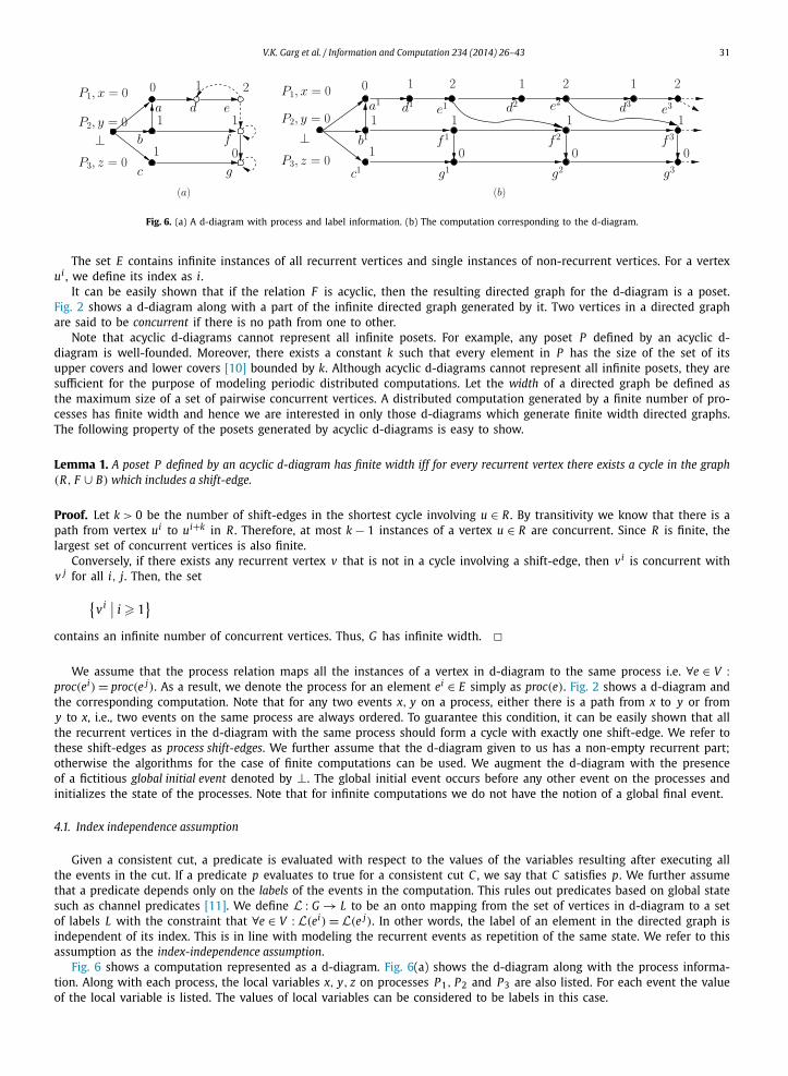
Fig. 6. (a) A d-diagram with process and label information. (b) The computation corresponding to the d-diagram.

The set E contains infinite instances of all recurrent vertices and single instances of non-recurrent vertices. For a vertexui , we define its index as i.

It can be easily shown that if the relation F is acyclic, then the resulting directed graph for the d-diagram is a poset.Fig. 2 shows a d-diagram along with a part of the infinite directed graph generated by it. Two vertices in a directed graphare said to be concurrent if there is no path from one to other.

Note that acyclic d-diagrams cannot represent all infinite posets. For example, any poset P defined by an acyclic d-diagram is well-founded. Moreover, there exists a constant k such that every element in P has the size of the set of itsupper covers and lower covers [10] bounded by k. Although acyclic d-diagrams cannot represent all infinite posets, they aresufficient for the purpose of modeling periodic distributed computations. Let the width of a directed graph be defined asthe maximum size of a set of pairwise concurrent vertices. A distributed computation generated by a finite number of pro-cesses has finite width and hence we are interested in only those d-diagrams which generate finite width directed graphs.The following property of the posets generated by acyclic d-diagrams is easy to show.

Lemma 1. A poset P defined by an acyclic d-diagram has finite width iff for every recurrent vertex there exists a cycle in the graph(R, F ∪ B) which includes a shift-edge.

Proof. Let k > 0 be the number of shift-edges in the shortest cycle involving u ∈ R . By transitivity we know that there is apath from vertex ui to ui+k in R . Therefore, at most k − 1 instances of a vertex u ∈ R are concurrent. Since R is finite, thelargest set of concurrent vertices is also finite.

Conversely, if there exists any recurrent vertex v that is not in a cycle involving a shift-edge, then vi is concurrent withv j for all i, j. Then, the set

{vi

∣∣ i � 1}

contains an infinite number of concurrent vertices. Thus, G has infinite width. �We assume that the process relation maps all the instances of a vertex in d-diagram to the same process i.e. ∀e ∈ V :

proc(ei) = proc(e j). As a result, we denote the process for an element ei ∈ E simply as proc(e). Fig. 2 shows a d-diagram andthe corresponding computation. Note that for any two events x, y on a process, either there is a path from x to y or fromy to x, i.e., two events on the same process are always ordered. To guarantee this condition, it can be easily shown that allthe recurrent vertices in the d-diagram with the same process should form a cycle with exactly one shift-edge. We refer tothese shift-edges as process shift-edges. We further assume that the d-diagram given to us has a non-empty recurrent part;otherwise the algorithms for the case of finite computations can be used. We augment the d-diagram with the presenceof a fictitious global initial event denoted by ⊥. The global initial event occurs before any other event on the processes andinitializes the state of the processes. Note that for infinite computations we do not have the notion of a global final event.

4.1. Index independence assumption

Given a consistent cut, a predicate is evaluated with respect to the values of the variables resulting after executing allthe events in the cut. If a predicate p evaluates to true for a consistent cut C , we say that C satisfies p. We further assumethat a predicate depends only on the labels of the events in the computation. This rules out predicates based on global statesuch as channel predicates [11]. We define L : G → L to be an onto mapping from the set of vertices in d-diagram to a setof labels L with the constraint that ∀e ∈ V : L(ei) = L(e j). In other words, the label of an element in the directed graph isindependent of its index. This is in line with modeling the recurrent events as repetition of the same state. We refer to thisassumption as the index-independence assumption.

Fig. 6 shows a computation represented as a d-diagram. Fig. 6(a) shows the d-diagram along with the process informa-tion. Along with each process, the local variables x, y, z on processes P1, P2 and P3 are also listed. For each event the valueof the local variable is listed. The values of local variables can be considered to be labels in this case.

32 V.K. Garg et al. / Information and Computation 234 (2014) 26–43

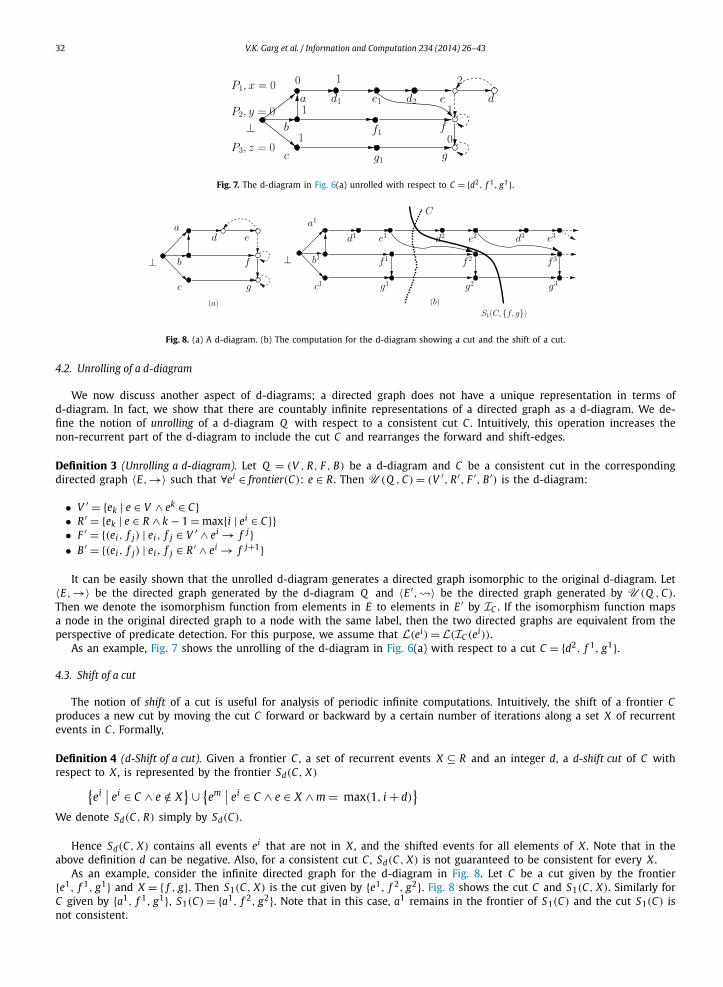
Fig. 7. The d-diagram in Fig. 6(a) unrolled with respect to C = {d2, f 1, g1}.

Fig. 8. (a) A d-diagram. (b) The computation for the d-diagram showing a cut and the shift of a cut.

4.2. Unrolling of a d-diagram

We now discuss another aspect of d-diagrams; a directed graph does not have a unique representation in terms ofd-diagram. In fact, we show that there are countably infinite representations of a directed graph as a d-diagram. We de-fine the notion of unrolling of a d-diagram Q with respect to a consistent cut C . Intuitively, this operation increases thenon-recurrent part of the d-diagram to include the cut C and rearranges the forward and shift-edges.

Definition 3 (Unrolling a d-diagram). Let Q = (V , R, F , B) be a d-diagram and C be a consistent cut in the correspondingdirected graph 〈E,→〉 such that ∀ei ∈ frontier(C): e ∈ R . Then U (Q , C) = (V ′, R ′, F ′, B ′) is the d-diagram:

• V ′ = {ek | e ∈ V ∧ ek ∈ C}• R ′ = {ek | e ∈ R ∧ k − 1 = max{i | ei ∈ C}}• F ′ = {(ei, f j) | ei, f j ∈ V ′ ∧ ei → f j}• B ′ = {(ei, f j) | ei, f j ∈ R ′ ∧ ei → f j+1}

It can be easily shown that the unrolled d-diagram generates a directed graph isomorphic to the original d-diagram. Let〈E,→〉 be the directed graph generated by the d-diagram Q and 〈E ′,�〉 be the directed graph generated by U (Q , C).Then we denote the isomorphism function from elements in E to elements in E ′ by IC . If the isomorphism function mapsa node in the original directed graph to a node with the same label, then the two directed graphs are equivalent from theperspective of predicate detection. For this purpose, we assume that L(ei) =L(IC (ei)).

As an example, Fig. 7 shows the unrolling of the d-diagram in Fig. 6(a) with respect to a cut C = {d2, f 1, g1}.

4.3. Shift of a cut

The notion of shift of a cut is useful for analysis of periodic infinite computations. Intuitively, the shift of a frontier Cproduces a new cut by moving the cut C forward or backward by a certain number of iterations along a set X of recurrentevents in C . Formally,

Definition 4 (d-Shift of a cut). Given a frontier C , a set of recurrent events X ⊆ R and an integer d, a d-shift cut of C withrespect to X , is represented by the frontier Sd(C, X)

{ei

∣∣ ei ∈ C ∧ e /∈ X} ∪ {

em∣∣ ei ∈ C ∧ e ∈ X ∧ m = max(1, i + d)

}

We denote Sd(C, R) simply by Sd(C).

Hence Sd(C, X) contains all events ei that are not in X , and the shifted events for all elements of X . Note that in theabove definition d can be negative. Also, for a consistent cut C , Sd(C, X) is not guaranteed to be consistent for every X .

As an example, consider the infinite directed graph for the d-diagram in Fig. 8. Let C be a cut given by the frontier{e1, f 1, g1} and X = { f , g}. Then S1(C, X) is the cut given by {e1, f 2, g2}. Fig. 8 shows the cut C and S1(C, X). Similarly forC given by {a1, f 1, g1}, S1(C) = {a1, f 2, g2}. Note that in this case, a1 remains in the frontier of S1(C) and the cut S1(C) isnot consistent.

V.K. Garg et al. / Information and Computation 234 (2014) 26–43 33

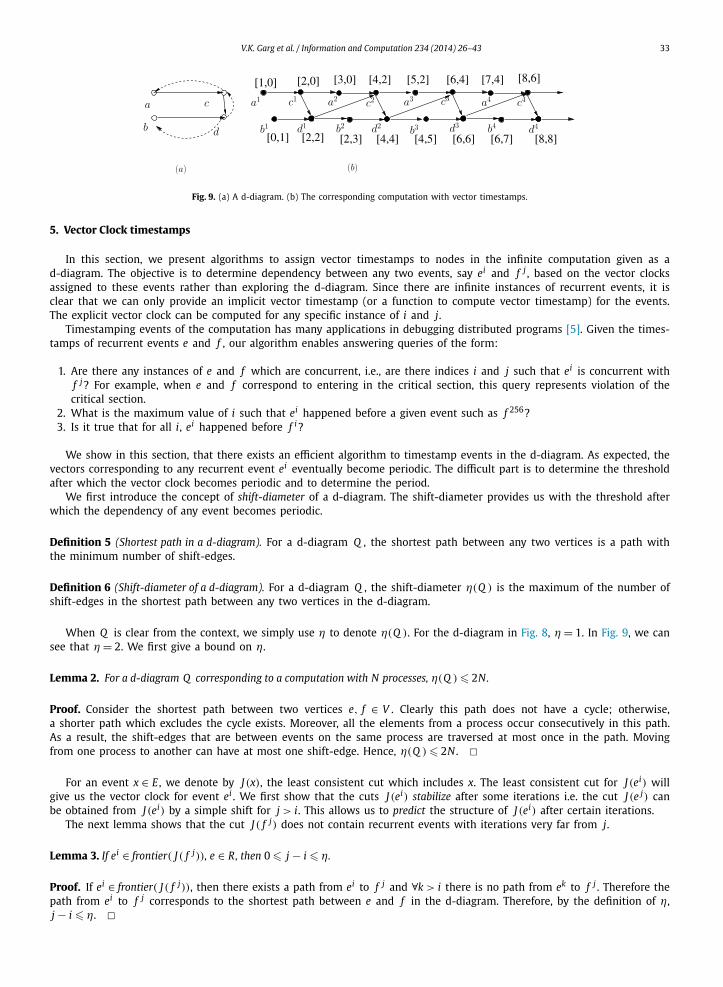
Fig. 9. (a) A d-diagram. (b) The corresponding computation with vector timestamps.

5. Vector Clock timestamps

In this section, we present algorithms to assign vector timestamps to nodes in the infinite computation given as ad-diagram. The objective is to determine dependency between any two events, say ei and f j , based on the vector clocksassigned to these events rather than exploring the d-diagram. Since there are infinite instances of recurrent events, it isclear that we can only provide an implicit vector timestamp (or a function to compute vector timestamp) for the events.The explicit vector clock can be computed for any specific instance of i and j.

Timestamping events of the computation has many applications in debugging distributed programs [5]. Given the times-tamps of recurrent events e and f , our algorithm enables answering queries of the form:

1. Are there any instances of e and f which are concurrent, i.e., are there indices i and j such that ei is concurrent withf j? For example, when e and f correspond to entering in the critical section, this query represents violation of thecritical section.

2. What is the maximum value of i such that ei happened before a given event such as f 256?3. Is it true that for all i, ei happened before f i ?

We show in this section, that there exists an efficient algorithm to timestamp events in the d-diagram. As expected, thevectors corresponding to any recurrent event ei eventually become periodic. The difficult part is to determine the thresholdafter which the vector clock becomes periodic and to determine the period.

We first introduce the concept of shift-diameter of a d-diagram. The shift-diameter provides us with the threshold afterwhich the dependency of any event becomes periodic.

Definition 5 (Shortest path in a d-diagram). For a d-diagram Q , the shortest path between any two vertices is a path withthe minimum number of shift-edges.

Definition 6 (Shift-diameter of a d-diagram). For a d-diagram Q , the shift-diameter η(Q ) is the maximum of the number ofshift-edges in the shortest path between any two vertices in the d-diagram.

When Q is clear from the context, we simply use η to denote η(Q ). For the d-diagram in Fig. 8, η = 1. In Fig. 9, we cansee that η = 2. We first give a bound on η.

Lemma 2. For a d-diagram Q corresponding to a computation with N processes, η(Q ) � 2N.

Proof. Consider the shortest path between two vertices e, f ∈ V . Clearly this path does not have a cycle; otherwise,a shorter path which excludes the cycle exists. Moreover, all the elements from a process occur consecutively in this path.As a result, the shift-edges that are between events on the same process are traversed at most once in the path. Movingfrom one process to another can have at most one shift-edge. Hence, η(Q )� 2N . �

For an event x ∈ E , we denote by J (x), the least consistent cut which includes x. The least consistent cut for J (ei) willgive us the vector clock for event ei . We first show that the cuts J (ei) stabilize after some iterations i.e. the cut J (e j) canbe obtained from J (ei) by a simple shift for j > i. This allows us to predict the structure of J (ei) after certain iterations.

The next lemma shows that the cut J ( f j) does not contain recurrent events with iterations very far from j.

Lemma 3. If ei ∈ frontier( J ( f j)), e ∈ R, then 0 � j − i � η.

Proof. If ei ∈ frontier( J ( f j)), then there exists a path from ei to f j and ∀k > i there is no path from ek to f j . Therefore thepath from ei to f j corresponds to the shortest path between e and f in the d-diagram. Therefore, by the definition of η,j − i � η. �

34 V.K. Garg et al. / Information and Computation 234 (2014) 26–43

The following theorem proves the result regarding the stabilization of the cut J (ei). Intuitively, after a first few iterationsthe relationship between elements of the computation depends only on the difference between their iterations.

Theorem 4. For a recurrent vertex e ∈ R, J (eβ+1) = S1( J (eβ)) for all β � η + 1.

Proof. We first show that S1( J (eβ)) ⊆ J (eβ+1). Consider f j ∈ S1( J (eβ)). If f ∈ V \ R (i.e., f is not a recurrent vertex),then f j ∈ J (eβ), because the shift operator affects only the recurrent vertices. This implies that there is a path from f j

to eβ , which in turn implies the path from f j to eβ+1. Hence, f j ∈ J (eβ+1). If f is recurrent, then f j ∈ S1( J (eβ)) impliesf j−1 ∈ J (eβ). This implies that there is a path from f j−1 to eβ , which in turn implies the path from f j to eβ+1, from theproperty of d-diagrams. Therefore, S1( J (eβ)) ⊆ J (eβ+1).

Now we show that J (eβ+1) ⊆ S1( J (eβ)). Consider f j ∈ J (eβ+1). If j > 1, then given a path from f j to eβ+1, there is apath from f j−1 to eβ . Hence f j ∈ S1( J (eβ)). Now, consider the case when j equals 1. f 1 ∈ J (eβ+1) implies that there is apath from f 1 to eβ+1. We claim that for β > η, there is also a path from f 1 to eβ . Otherwise, the shortest path from f toe has more than η shift-edges, a contradiction. �

When d-diagram generates a poset, Theorem 4 can be used to assign timestamps to vertices in the d-diagram in a waysimilar to vector clocks. The difference here is that a timestamp for a recurrent vertex is a concise way of representing thetimestamps of infinite instances of that vertex.

Each recurrent event, e, has a special p-timestamp (P V (e)) associated with it, which lets us compute the time stamp forany arbitrary iteration of that event. Therefore, this result gives us an algorithm for assigning p-timestamp to a recurrentevent. The p-timestamp for a recurrent event e, P V (e) would be a list of the form

(V

(e1), . . . , V

(eβ

); I(e))

where I(e) = V (eβ+1) − V (eβ) and V (e j) is the timestamp assigned by the normal vector clock algorithm to event e j . Nowfor any event e j, j > β , V (e j) = V (eβ) + ( j − β) ∗ I(e).

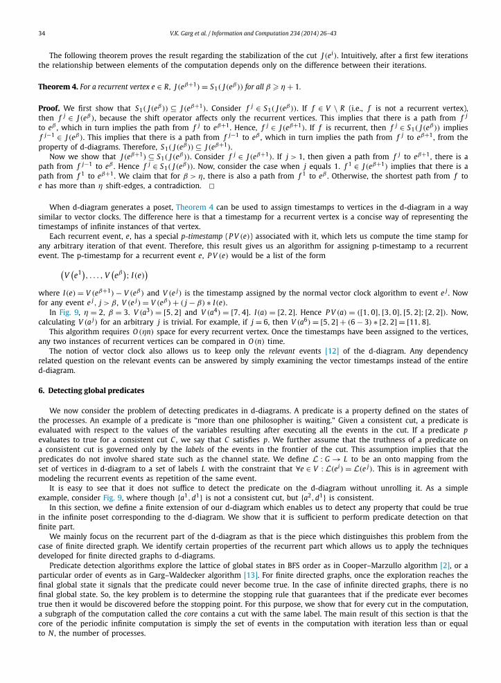
In Fig. 9, η = 2, β = 3. V (a3) = [5,2] and V (a4) = [7,4]. I(a) = [2,2]. Hence P V (a) = ([1,0], [3,0], [5,2]; [2,2]). Now,calculating V (a j) for an arbitrary j is trivial. For example, if j = 6, then V (a6) = [5,2] + (6 − 3) ∗ [2,2] = [11,8].

This algorithm requires O (ηn) space for every recurrent vertex. Once the timestamps have been assigned to the vertices,any two instances of recurrent vertices can be compared in O (n) time.

The notion of vector clock also allows us to keep only the relevant events [12] of the d-diagram. Any dependencyrelated question on the relevant events can be answered by simply examining the vector timestamps instead of the entired-diagram.

6. Detecting global predicates

We now consider the problem of detecting predicates in d-diagrams. A predicate is a property defined on the states ofthe processes. An example of a predicate is “more than one philosopher is waiting.” Given a consistent cut, a predicate isevaluated with respect to the values of the variables resulting after executing all the events in the cut. If a predicate pevaluates to true for a consistent cut C , we say that C satisfies p. We further assume that the truthness of a predicate ona consistent cut is governed only by the labels of the events in the frontier of the cut. This assumption implies that thepredicates do not involve shared state such as the channel state. We define L : G → L to be an onto mapping from theset of vertices in d-diagram to a set of labels L with the constraint that ∀e ∈ V : L(ei) = L(e j). This is in agreement withmodeling the recurrent events as repetition of the same event.

It is easy to see that it does not suffice to detect the predicate on the d-diagram without unrolling it. As a simpleexample, consider Fig. 9, where though {a1,d1} is not a consistent cut, but {a2,d1} is consistent.

In this section, we define a finite extension of our d-diagram which enables us to detect any property that could be truein the infinite poset corresponding to the d-diagram. We show that it is sufficient to perform predicate detection on thatfinite part.

We mainly focus on the recurrent part of the d-diagram as that is the piece which distinguishes this problem from thecase of finite directed graph. We identify certain properties of the recurrent part which allows us to apply the techniquesdeveloped for finite directed graphs to d-diagrams.

Predicate detection algorithms explore the lattice of global states in BFS order as in Cooper–Marzullo algorithm [2], or aparticular order of events as in Garg–Waldecker algorithm [13]. For finite directed graphs, once the exploration reaches thefinal global state it signals that the predicate could never become true. In the case of infinite directed graphs, there is nofinal global state. So, the key problem is to determine the stopping rule that guarantees that if the predicate ever becomestrue then it would be discovered before the stopping point. For this purpose, we show that for every cut in the computation,a subgraph of the computation called the core contains a cut with the same label. The main result of this section is that thecore of the periodic infinite computation is simply the set of events in the computation with iteration less than or equalto N , the number of processes.

V.K. Garg et al. / Information and Computation 234 (2014) 26–43 35

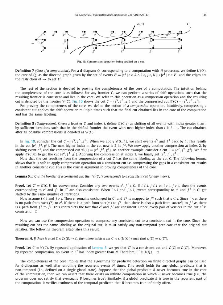
Fig. 10. Compression operation being applied on a cut.

Definition 7 (Core of a computation). For a d-diagram Q corresponding to a computation with N processes, we define U (Q ),the core of Q , as the directed graph given by the set of events E ′ = {e j | e ∈ R ∧ 2 � j � N} ∪ {e1 | e ∈ V } and the edges arethe restriction of → to set E ′ .

The rest of the section is devoted to proving the completeness of the core of a computation. The intuition behindthe completeness of the core is as follows: For any frontier C , we can perform a series of shift operations such that theresulting frontier is consistent and lies in the core. We refer to this operation as a compression operation and the resultingcut is denoted by the frontier C (C). Fig. 10 shows the cut C = {e5, f 3, g1} and the compressed cut C (C) = {e3, f 2, g1}.

For proving the completeness of the core, we define the notion of a compression operation. Intuitively, compressing aconsistent cut applies the shift operation multiple times such that the final cut obtained lies in the core of the computationand has the same labeling.

Definition 8 (Compression). Given a frontier C and index i, define C (C, i) as shifting of all events with index greater than iby sufficient iterations such that in the shifted frontier the event with next higher index than i is i + 1. The cut obtainedafter all possible compressions is denoted as C (C).

In Fig. 10, consider the cut C = {e5, f 3, g1}. When we apply C (C,1), we shift events e5 and f 3 back by 1. This resultsin the cut {e4, f 2, g1}. The next higher index in the cut now is 2 in f 2. We now apply another compression at index 2, byshifting event e4, and the compressed cut C (C) = {e3, f 2, g1}. As another example, consider a cut C = {e7, f 4, g4}. We firstapply C (C,0) to get the cut {e4, f 1, g1}. Applying the compression at index 1, we finally get {e2, f 1, g1}.

Note that the cut resulting from the compression of a cut C has the same labeling as the cut C . The following lemmashows that it is safe to apply compression operation on a consistent cut i.e. compressing the gaps in a consistent cut resultsin another consistent cut. This is the crucial argument in proving completeness of the core.

Lemma 5. If C is the frontier of a consistent cut, then C (C, l) corresponds to a consistent cut for any index l.

Proof. Let C ′ = C (C, l) for convenience. Consider any two events ei, f j ∈ C . If i � l, j � l or i > l, j > l, then the eventscorresponding to ei and f j in C ′ are also consistent. When i > l and j > l, events corresponding to ei and f j in C ′ getshifted by the same number of iterations.

Now assume i � l and j > l. Then ei remains unchanged in C ′ and f j is mapped to f a such that a � j. Since i < a, thereis no path from succ( f a) to ei . If there is a path from succ(ei) to f a , then there is also a path from succ(ei) to f j as thereis a path from f a to f j . This contradicts the fact that ei and f j are consistent. Hence, every pair of vertices in the cut C ′ isconsistent. �

Now we can use the compression operation to compress any consistent cut to a consistent cut in the core. Since theresulting cut has the same labeling as the original cut, it must satisfy any non-temporal predicate that the original cutsatisfies. The following theorem establishes this result.

Theorem 6. If there is a cut C ∈ C(〈E,→〉), then there exists a cut C ′ ∈ C(U (Q )) such that L(C) =L(C ′).

Proof. Let C ′ = C (C). By repeated application of Lemma 5, we get that C ′ is a consistent cut and L(C) = L(C ′). Moreover,by repeated compression, no event in C ′ has index greater than N . Therefore, C ′ ∈ U (Q ). �

The completeness of the core implies that the algorithms for predicate detection on finite directed graphs can be usedfor d-diagrams as well after unrolling the recurrent events N times. This result holds for any global predicate that isnon-temporal (i.e., defined on a single global state). Suppose that the global predicate B never becomes true in the coreof the computation, then we can assert that there exists an infinite computation in which B never becomes true (i.e., theprogram does not satisfy that eventually B becomes true). Similarly, if a global predicate B is true in the recurrent part ofthe computation, it verifies truthness of the temporal predicate that B becomes true infinitely often.

36 V.K. Garg et al. / Information and Computation 234 (2014) 26–43

7. Recurrent global state detection algorithm

We now briefly discuss a method to obtain a d-diagram from a finite distributed computation. The local state of a processis the value of all the variables of the process including the program counter. The channel state between two processes is thesequence of messages that have been sent on the channel but not received. A global state of a computation is defined to bethe cross product of local states of all processes and all the channel states at any cut. Any consistent cut of the computationdetermines a unique consistent global state. A global state is recurrent in a computation, if there exist consistent cuts Y andZ such that the global states for Y and Z are identical and Y is a proper subset of Z . Informally, a global state is recurrentif there are at least two distinct instances of that global state in the computation.

We now give an algorithm to detect recurrent global states of a computation. We assume that the system logs themessage order and nondeterministic events so that the distributed computation can be exactly replayed. We also assumethat the system supports a vector clock mechanism.

The first step of our recurrent global state detection (RGSD) algorithm consists of computing the global state of a dis-tributed system. Assuming FIFO, we could use the classical Chandy and Lamport’s algorithm [1] for this purpose. Otherwise,we can use any of the algorithms, such as [14–16]. Let the computed global snapshot be G . Let Z be the vector clock forthe global state G .

The second step consists of replaying the distributed computation while monitoring the computation to determine theleast consistent cut that matches G . We are guaranteed to hit such a global state because there exists at least one suchglobal state (at vector time Z ) in the computation. Suppose that the vector clock of the detected global state is Y . We nowhave two vector clocks Y and Z corresponding to the global state G . If Y equals Z , we continue with our computation.Otherwise, we have succeeded in finding a recurrent global state G .

Note that replaying a distributed computation requires that all nondeterministic events (including the message order) berecorded during the initial execution [17]. Monitoring the computation to determine the least consistent cut that matchesG can be done using algorithms for conjunctive predicate detection [3,11].

When the second step fails to find a recurrent global state, the first step of the algorithm is invoked again after certaintime interval. We make the following observation about the recurrent global state detection algorithm.

Theorem 7. If the distributed computation is periodic then the algorithm will detect a recurrent global state. Conversely, if the algorithmreturns a recurrent global state G, then there exists an infinite computation in which G appears infinitely often.

Proof. The RGSD algorithm is invoked periodically and therefore it will be invoked at least once in repetitive part of thecomputation. This invocation will compute a global state G . Since the computation is now in repetitive mode, the globalstate G must have occurred earlier and the RGSD algorithm will declare G as a recurrent global state.

We prove the converse by constructing the infinite computation explicitly. Let Y and Z be the vector clocks correspond-ing to the recurrent global state G . Our infinite computation will first execute all events till Y . After that it will executethe computation that corresponds to events executed between Y and Z . Since Y and Z have identical global state, thecomputation after Y is also a legal computation after Z . By repeatedly executing this computation, we get an infinite legalcomputation in which G appears infinitely often. �

The proof of Theorem 7 also shows how we can construct a p-diagram given the recurrent global state G . Let Y and Zbe the vector clocks corresponding to the global state G . All the events between Y and Z are modeled as recurrent vertices.For every process, we add shift-edges from the last event in Z to the first event after Y on that process. In addition, forevery message that is in channel at the global state in Z , we add a shift edge from the send event on the sending processto the receive event. An example of this construction is Fig. 5. The global state after β and β followed by γ are recurrent.The computation in Fig: 9(a) shows an example in which the shift edge in p-diagram is from one process to the other.

It is important to note that our algorithm does not guarantee that if there exists any recurrent global state, it will bedetected by the algorithm. It only guarantees that if the computation is periodic, then it will be detected.

We note here that RGSD algorithm is also useful in debugging applications in which the distributed program is supposedto be terminating and presence of a recurrent global state itself indicates a bug.

8. Computing slice of a computation

In this section we present an algorithm to compute slice of a periodic computation. We first provide a brief introductionto slicing, then we generalize the notion of d-diagrams by introducing k-shift-edges because the slice is more convenientlyexpressed using generalized d-diagram. Then, we give an algorithm to compute the slice.

8.1. Background on slicing

In the earlier work [7,8], the notion of slicing was used for finite directed graphs and was based on Birkhoff’s representa-tion theorem for finite distributive lattices [18]. Informally, a computation slice (or simply a slice) is a concise representationof all those consistent cuts of the computation that satisfy the predicate.

V.K. Garg et al. / Information and Computation 234 (2014) 26–43 37

In this work, we extend the notion of slicing for infinite directed graphs by focusing only on finite order ideals [18].As mentioned earlier as well, we deal only with finite consistent cuts and refer to them simply as consistent cuts. Similarto Birkhoff’s representation theorem [18], the following theorem is known for the case of finite order ideals of an infiniteposet:

Theorem 8. (See [19], Proposition 3.4.3.) Let P be a poset such that every principal order ideal is finite. Then the poset J f (P ) of finiteorder ideals of P , ordered by inclusion, is a finitary distributive lattice. Conversely, if L is a finitary distributive lattice and P is itssubposet of join-irreducibles, then every principal order ideal of P is finite and L = J f (P ).

We can use the above theorem instead of Birkhoff’s theorem and generalize the notion of slice for consistent cuts to thefollowing definition.

Definition 9 (Slice). The slice of a directed graph G with respect to a predicate p is the directed graph whose consistentcuts form the smallest sublattice that contains all the consistent cuts satisfying the predicate p.

This definition is equivalent to the definition of slice in the earlier work for finite directed graphs. It can be easily shownthat the slice for a predicate always exists and is unique. Since the slice of an infinite directed graph can again be aninfinite directed graph, we use d-diagram to represent the slice of a computation as well. We later show that if the originalcomputation was representable using d-diagram, then the slice of the computation is also representable by d-diagram.

We denote the slice of the computation 〈E,→〉 with respect to a predicate p by slice(〈E,→〉, p). Note that〈E,→〉 = slice(〈E,→〉, true). Every slice derived from the computation 〈E,→〉 has the trivial consistent cut ∅ among itsset of consistent cuts. A slice is empty if it has no non-trivial consistent cuts [8]. In the rest of the paper, unless otherwisestated, a consistent cut refers to a non-trivial consistent cut.

In general, a slice contains consistent cuts that do not satisfy the predicate (besides trivial consistent cut ∅). In case aslice does not contain any such cut, it is called lean. The slice for the class of predicates called regular predicates is alwayslean. Given a computation, the set of consistent cuts satisfying a regular predicate forms a sublattice of the set of consistentcuts of the computation [7]. Equivalently,

Definition 10 (Regular predicate). (See [7].) A predicate is regular if given two consistent cuts that satisfy the predicate,the consistent cuts obtained by their set union and set intersection also satisfy the predicate. Formally, given a regularpredicate p,

(C satisfies p) ∧ (D satisfies p) ⇒ (C ∩ D satisfies p) ∧ (C ∪ D satisfies p)

Some examples of regular predicates are conjunction of local predicates such as “Pi and P j are in critical section”, andrelational predicates such as x1 − x2 � 5, where xi is a monotonically non-decreasing integer variable on process Pi . Fromthe definition of a regular predicate we deduce that a regular predicate has a least satisfying cut as the lattice of orderideals has a bottom element. Furthermore, the class of regular predicates is closed under conjunction [7].

For a regular predicate p and an element x ∈ G , we define J p(x) as the least consistent cut which satisfies p andincludes x. If there is no cut that satisfies p and includes x, J p(x) is defined to be NULL; otherwise J p(x) is well-defined asthe regular predicates are closed under intersection.

8.2. Generalized d-diagram

For computing slice of a d-diagram it is covenient to first generalize the d-diagrams by having k-shift-edges whichincrease the iteration of a vertex by k for any arbitrary k instead of a simple shift-edge. We call such a d-diagram as thegeneralized d-diagram.

Definition 11 (Generalized d-diagram). A generalized d-diagram is a set (V , R, F , B1, B2, . . . , Bm) where m is the maximumk such that a k-shift-edges is present in the d-diagram and Bk ⊆ (V × R) is the relation of k-shift-edges with the property: If(e, f ) ∈ Bk , then ei → f i+k .

Note that in the above definition, we allow the shift edges to be present between non-recurrent and recurrent verticesas well. Clearly d-diagrams are a special case of the generalized d-diagrams where m = 1 and B1 ⊆ R × R . The followingtheorem further shows that the generalized d-diagram are not any more expressive than the d-diagrams.

Theorem 9. Let (V , R, F , B1, B2, . . . , Bm) be a generalized d-diagram and 〈E,→〉 be the infinite graph generated by it. Then thereexists a d-diagram (V ′, R ′, F ′, B ′) such that the graph 〈E ′,�〉 generated by the d-diagram is isomorphic to the graph 〈E,→〉.

Proof. We construct the d-diagram corresponding to the generalized d-diagram as follows.

38 V.K. Garg et al. / Information and Computation 234 (2014) 26–43

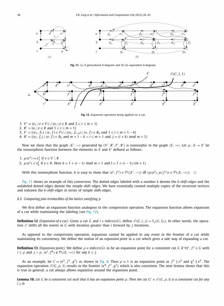
Fig. 11. (a) A generalized d-diagram and (b) its equivalent d-diagram.

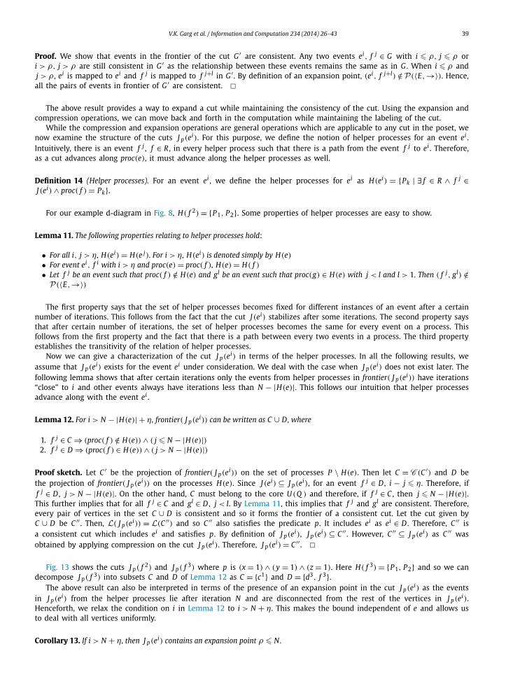
Fig. 12. Expansion operation being applied on a cut.

1. V ′ = {e1 | e ∈ V } ∪ {ei | e ∈ R and 2 � i � m + 1}2. R ′ = {ei | e ∈ R and 1 � i � m + 1}3. F ′ = {(e1, f1) | (e, f ) ∈ F } ∪ {(ei, f i+k) | (e, f ) ∈ Bk and 1 � i � m + 1 − k}4. B ′ = {(ei, f j) | (e, f ) ∈ Bk and m + 1 − k < i � m + 1 and j = (i + k) mod m + 1}

Now we show that the graph 〈E ′,�〉 generated by (V ′, R ′, F ′, B ′) is isomorphic to the graph 〈E,→〉. Let μ : E → E ′ bethe isomorphism function between the elements in E and E ′ defined as follows:

1. μ(e1) = e11 if e ∈ V \ R

2. μ(ei) = elk if e ∈ R . Here k = 1 + (i − 1) mod m + 1 and l = 1 + (i − 1)/(m + 1)

With this isomorphism function, it is easy to show that (ei, f j) ∈P(〈E ′,�〉) iff (μ(ei),μ( f j)) ∈P(〈E,→〉). �Fig. 11 shows an example of this conversion. The dotted edges labeled with a number k denote the k-shift-edges and the

unlabeled dotted edges denote the simple shift edges. We have essentially created multiple copies of the recurrent verticesand redrawn the k-shift-edges in terms of simple shift-edges.

8.3. Computing join-irreducibles of the lattice satisfying p

We first define an expansion function analogous to the compression operation. The expansion function allows expansionof a cut while maintaining the labeling (see Fig. 12).

Definition 12 (Expansion of a cut). Given a cut G and i ∈ indices(G), define E (G, i, j) = S j(G, Gi). In other words, the opera-tion E shifts all the events in G with iteration greater than i forward by j iterations.

As opposed to the compression operation, expansion cannot be applied to any event in the frontier of a cut whilemaintaining its consistency. We define the notion of an expansion point in a cut which gives a safe way of expanding a cut.

Definition 13 (Expansion point). We define ρ ∈ indices(G) to be an expansion point for a consistent cut G if ∀ei, f j ∈ G withi � ρ and j > ρ , (ei, f k) /∈P(〈E,→〉) for any k � j.

As an example, let C = {e3, f 1, g1} as shown in Fig. 8. Then ρ = 1 is an expansion point as f 1 ‖ e3 and g1 ‖ e3. Theexpansion operation E (G,ρ,1) results in the frontier {e4, f 1, g1} which is also consistent. The next lemma shows that thisis true in general; a cut always allows expansion around the expansion point.

Lemma 10. Let G be a consistent cut such that it has an expansion point ρ . Then the cut G ′ = E (G,ρ, l) is a consistent cut for anyl � 0.

V.K. Garg et al. / Information and Computation 234 (2014) 26–43 39

Proof. We show that events in the frontier of the cut G ′ are consistent. Any two events ei, f j ∈ G with i � ρ, j � ρ ori > ρ, j > ρ are still consistent in G ′ as the relationship between these events remains the same as in G . When i � ρ andj > ρ , ei is mapped to ei and f j is mapped to f j+l in G ′ . By definition of an expansion point, (ei, f j+l) /∈P(〈E,→〉). Hence,all the pairs of events in frontier of G ′ are consistent. �

The above result provides a way to expand a cut while maintaining the consistency of the cut. Using the expansion andcompression operations, we can move back and forth in the computation while maintaining the labeling of the cut.

While the compression and expansion operations are general operations which are applicable to any cut in the poset, wenow examine the structure of the cuts J p(ei). For this purpose, we define the notion of helper processes for an event ei .Intuitively, there is an event f j , f ∈ R , in every helper process such that there is a path from the event f j to ei . Therefore,as a cut advances along proc(e), it must advance along the helper processes as well.

Definition 14 (Helper processes). For an event ei , we define the helper processes for ei as H(ei) = {Pk | ∃ f ∈ R ∧ f j ∈J (ei) ∧ proc( f ) = Pk}.

For our example d-diagram in Fig. 8, H( f 2) = {P1, P2}. Some properties of helper processes are easy to show.

Lemma 11. The following properties relating to helper processes hold:

• For all i, j > η, H(ei) = H(e j). For i > η, H(ei) is denoted simply by H(e)• For event ei, f i with i > η and proc(e) = proc( f ), H(e) = H( f )• Let f j be an event such that proc( f ) /∈ H(e) and gl be an event such that proc(g) ∈ H(e) with j < l and l > 1. Then ( f j, gl) /∈P(〈E,→〉)

The first property says that the set of helper processes becomes fixed for different instances of an event after a certainnumber of iterations. This follows from the fact that the cut J (ei) stabilizes after some iterations. The second property saysthat after certain number of iterations, the set of helper processes becomes the same for every event on a process. Thisfollows from the first property and the fact that there is a path between every two events in a process. The third propertyestablishes the transitivity of the relation of helper processes.

Now we can give a characterization of the cut J p(ei) in terms of the helper processes. In all the following results, weassume that J p(ei) exists for the event ei under consideration. We deal with the case when J p(ei) does not exist later. Thefollowing lemma shows that after certain iterations only the events from helper processes in frontier( J p(ei)) have iterations“close” to i and other events always have iterations less than N − |H(e)|. This follows our intuition that helper processesadvance along with the event ei .

Lemma 12. For i > N − |H(e)| + η, frontier( J p(ei)) can be written as C ∪ D, where

1. f j ∈ C ⇒ (proc( f ) /∈ H(e)) ∧ ( j � N − |H(e)|)2. f j ∈ D ⇒ (proc( f ) ∈ H(e)) ∧ ( j > N − |H(e)|)

Proof sketch. Let C ′ be the projection of frontier( J p(ei)) on the set of processes P \ H(e). Then let C = C (C ′) and D bethe projection of frontier( J p(ei)) on the processes H(e). Since J (ei) ⊆ J p(ei), for an event f j ∈ D , i − j � η. Therefore, iff j ∈ D , j > N − |H(e)|. On the other hand, C must belong to the core U (Q ) and therefore, if f j ∈ C , then j � N − |H(e)|.This further implies that for all f j ∈ C and gl ∈ D , j < l. By Lemma 11, this implies that f j and gl are consistent. Therefore,every pair of vertices in the set C ∪ D is consistent and so it forms the frontier of a consistent cut. Let the cut given byC ∪ D be C ′′ . Then, L( J p(ei)) = L(C ′′) and so C ′′ also satisfies the predicate p. It includes ei as ei ∈ D . Therefore, C ′′ isa consistent cut which includes ei and satisfies p. By definition of J p(ei), J p(ei) ⊆ C ′′ . However, C ′′ ⊆ J p(ei) as C ′′ wasobtained by applying compression on the cut J p(ei). Therefore, J p(ei) = C ′′ . �

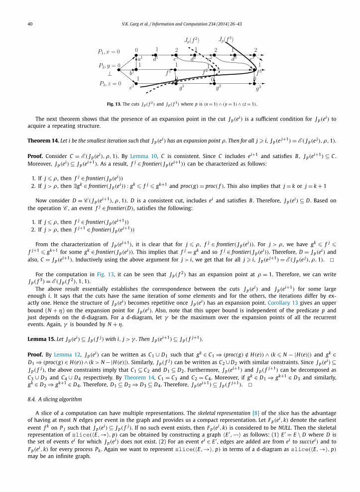
Fig. 13 shows the cuts J p( f 2) and J p( f 3) where p is (x = 1) ∧ (y = 1) ∧ (z = 1). Here H( f 3) = {P1, P2} and so we candecompose J p( f 3) into subsets C and D of Lemma 12 as C = {c1} and D = {d3, f 3}.

The above result can also be interpreted in terms of the presence of an expansion point in the cut J p(ei) as the eventsin J p(ei) from the helper processes lie after iteration N and are disconnected from the rest of the vertices in J p(ei).Henceforth, we relax the condition on i in Lemma 12 to i > N + η. This makes the bound independent of e and allows usto deal with all vertices uniformly.

Corollary 13. If i > N + η, then J p(ei) contains an expansion point ρ � N.

40 V.K. Garg et al. / Information and Computation 234 (2014) 26–43

Fig. 13. The cuts J p( f 2) and J p( f 3) where p is (x = 1) ∧ (y = 1) ∧ (z = 1).

The next theorem shows that the presence of an expansion point in the cut J p(ei) is a sufficient condition for J p(ei) toacquire a repeating structure.

Theorem 14. Let i be the smallest iteration such that J p(ei) has an expansion point ρ . Then for all j � i, J p(e j+1) = E ( J p(e j),ρ,1).

Proof. Consider C = E ( J p(ei),ρ,1). By Lemma 10, C is consistent. Since C includes ei+1 and satisfies B , J p(ei+1) ⊆ C .Moreover, J p(ei) ⊆ J p(ei+1). As a result, f j ∈ frontier( J p(ei+1)) can be characterized as follows:

1. If j � ρ , then f j ∈ frontier( J p(ei))

2. If j > ρ , then ∃gk ∈ frontier( J p(ei)) : gk � f j � gk+1 and proc(g) = proc( f ). This also implies that j = k or j = k + 1

Now consider D = C ( J p(ei+1),ρ,1). D is a consistent cut, includes ei and satisfies B . Therefore, J p(ei) ⊆ D . Based onthe operation C , an event f j ∈ frontier(D), satisfies the following:

1. If j � ρ , then f j ∈ frontier( J p(ei+1))

2. If j > ρ , then f j+1 ∈ frontier( J p(ei+1))

From the characterization of J p(ei+1), it is clear that for j � ρ , f j ∈ frontier( J p(ei)). For j > ρ , we have gk � f j �f j+1 � gk+1 for some gk ∈ frontier( J p(ei)). This implies that f j = gk and so f j ∈ frontier( J p(ei)). Therefore, D = J p(ei) andalso, C = J p(ei+1). Inductively using the above argument for j > i, we get that for all j � i, J p(e j+1) = E ( J p(e j),ρ,1). �

For the computation in Fig. 13, it can be seen that J p( f 2) has an expansion point at ρ = 1. Therefore, we can writeJ p( f 3) = E ( J p( f 2),1,1).

The above result essentially establishes the correspondence between the cuts J p(ei) and J p(ei+1) for some largeenough i. It says that the cuts have the same iteration of some elements and for the others, the iterations differ by ex-actly one. Hence the structure of J p(ei) becomes repetitive once J p(ei) has an expansion point. Corollary 13 gives an upperbound (N + η) on the expansion point for J p(ei). Also, note that this upper bound is independent of the predicate p andjust depends on the d-diagram. For a d-diagram, let γ be the maximum over the expansion points of all the recurrentevents. Again, γ is bounded by N + η.

Lemma 15. Let J p(ei) ⊆ J p( f j) with i, j > γ . Then J p(ei+1) ⊆ J p( f j+1).

Proof. By Lemma 12, J p(ei) can be written as C1 ∪ D1 such that gk ∈ C1 ⇒ (proc(g) /∈ H(e)) ∧ (k � N − |H(e)|) and gk ∈D1 ⇒ (proc(g) ∈ H(e))∧ (k > N −|H(e)|). Similarly, J p( f j) can be written as C2 ∪ D2 with similar constraints. Since J p(ei) ⊆J p( f j), the above constraints imply that C1 ⊆ C2 and D1 ⊆ D2. Furthermore, J p(ei+1) and J p( f j+1) can be decomposed asC3 ∪ D3 and C4 ∪ D4 respectively. By Theorem 14, C1 = C3 and C2 = C4. Moreover, if gk ∈ D1 ⇒ gk+1 ∈ D3 and similarly,gk ∈ D2 ⇒ gk+1 ∈ D4. Therefore, D1 ⊆ D2 ⇒ D3 ⊆ D4. Therefore, J p(ei+1) ⊆ J p( f j+1). �8.4. A slicing algorithm

A slice of a computation can have multiple representations. The skeletal representation [8] of the slice has the advantageof having at most N edges per event in the graph and provides us a compact representation. Let F p(ei,k) denote the earliestevent f k on P j such that J p(ei) ⊆ J p( f j). If no such event exists, then F p(ei,k) is considered to be NULL. Then the skeletalrepresentation of slice(〈E,→〉, p) can be obtained by constructing a graph 〈E ′,�〉 as follows: (1) E ′ = E \ D where D isthe set of events ei for which J p(ei) does not exist. (2) For an event ei ∈ E ′ , edges are added are from ei to succ(ei) and toF p(ei,k) for every process Pk . Again we want to represent slice(〈E,→〉, p) in terms of a d-diagram as slice(〈E,→〉, p)

may be an infinite graph.

V.K. Garg et al. / Information and Computation 234 (2014) 26–43 41

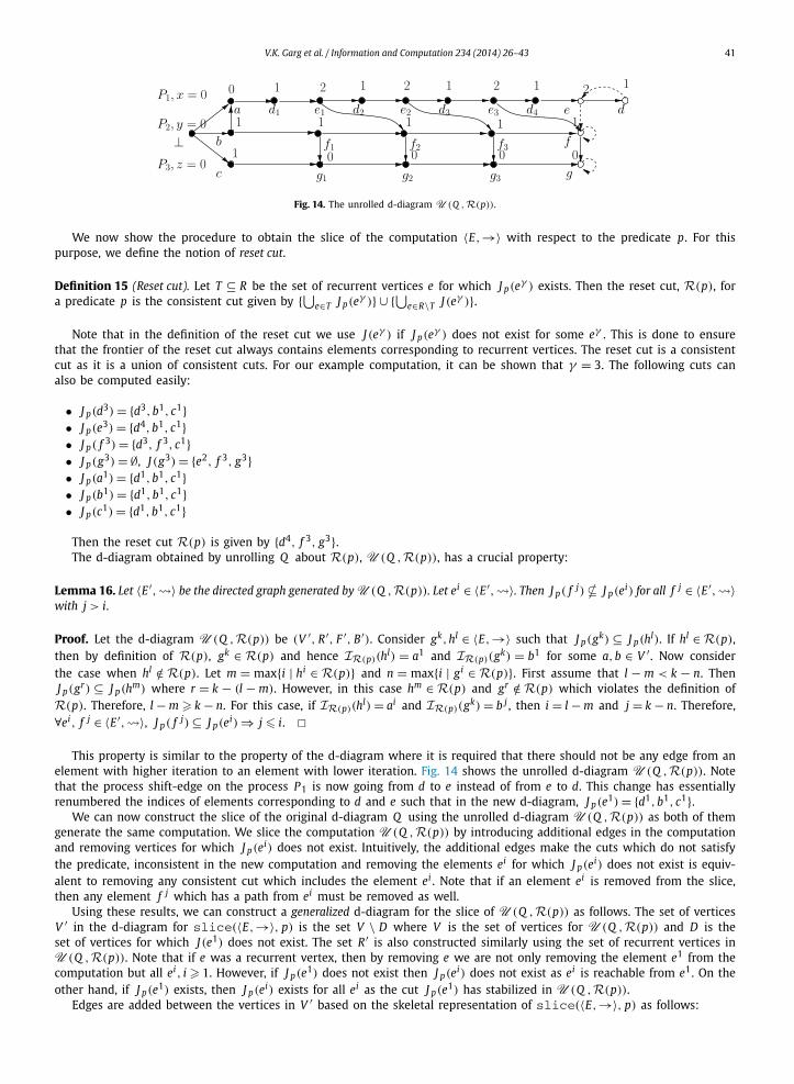
Fig. 14. The unrolled d-diagram U (Q ,R(p)).

We now show the procedure to obtain the slice of the computation 〈E,→〉 with respect to the predicate p. For thispurpose, we define the notion of reset cut.

Definition 15 (Reset cut). Let T ⊆ R be the set of recurrent vertices e for which J p(eγ ) exists. Then the reset cut, R(p), fora predicate p is the consistent cut given by {⋃e∈T J p(eγ )} ∪ {⋃e∈R\T J (eγ )}.

Note that in the definition of the reset cut we use J (eγ ) if J p(eγ ) does not exist for some eγ . This is done to ensurethat the frontier of the reset cut always contains elements corresponding to recurrent vertices. The reset cut is a consistentcut as it is a union of consistent cuts. For our example computation, it can be shown that γ = 3. The following cuts canalso be computed easily:

• J p(d3) = {d3,b1, c1}• J p(e3) = {d4,b1, c1}• J p( f 3) = {d3, f 3, c1}• J p(g3) = ∅, J (g3) = {e2, f 3, g3}• J p(a1) = {d1,b1, c1}• J p(b1) = {d1,b1, c1}• J p(c1) = {d1,b1, c1}

Then the reset cut R(p) is given by {d4, f 3, g3}.The d-diagram obtained by unrolling Q about R(p), U (Q ,R(p)), has a crucial property:

Lemma 16. Let 〈E ′,�〉 be the directed graph generated by U (Q ,R(p)). Let ei ∈ 〈E ′,�〉. Then J p( f j) � J p(ei) for all f j ∈ 〈E ′,�〉with j > i.

Proof. Let the d-diagram U (Q ,R(p)) be (V ′, R ′, F ′, B ′). Consider gk,hl ∈ 〈E,→〉 such that J p(gk) ⊆ J p(hl). If hl ∈ R(p),then by definition of R(p), gk ∈ R(p) and hence IR(p)(hl) = a1 and IR(p)(gk) = b1 for some a,b ∈ V ′ . Now considerthe case when hl /∈ R(p). Let m = max{i | hi ∈ R(p)} and n = max{i | gi ∈ R(p)}. First assume that l − m < k − n. ThenJ p(gr) ⊆ J p(hm) where r = k − (l − m). However, in this case hm ∈ R(p) and gr /∈ R(p) which violates the definition ofR(p). Therefore, l − m � k − n. For this case, if IR(p)(hl) = ai and IR(p)(gk) = b j , then i = l − m and j = k − n. Therefore,∀ei, f j ∈ 〈E ′,�〉, J p( f j) ⊆ J p(ei) ⇒ j � i. �

This property is similar to the property of the d-diagram where it is required that there should not be any edge from anelement with higher iteration to an element with lower iteration. Fig. 14 shows the unrolled d-diagram U (Q ,R(p)). Notethat the process shift-edge on the process P1 is now going from d to e instead of from e to d. This change has essentiallyrenumbered the indices of elements corresponding to d and e such that in the new d-diagram, J p(e1) = {d1,b1, c1}.

We can now construct the slice of the original d-diagram Q using the unrolled d-diagram U (Q ,R(p)) as both of themgenerate the same computation. We slice the computation U (Q ,R(p)) by introducing additional edges in the computationand removing vertices for which J p(ei) does not exist. Intuitively, the additional edges make the cuts which do not satisfythe predicate, inconsistent in the new computation and removing the elements ei for which J p(ei) does not exist is equiv-alent to removing any consistent cut which includes the element ei . Note that if an element ei is removed from the slice,then any element f j which has a path from ei must be removed as well.

Using these results, we can construct a generalized d-diagram for the slice of U (Q ,R(p)) as follows. The set of verticesV ′ in the d-diagram for slice(〈E,→〉, p) is the set V \ D where V is the set of vertices for U (Q ,R(p)) and D is theset of vertices for which J (e1) does not exist. The set R ′ is also constructed similarly using the set of recurrent vertices inU (Q ,R(p)). Note that if e was a recurrent vertex, then by removing e we are not only removing the element e1 from thecomputation but all ei, i � 1. However, if J p(e1) does not exist then J p(ei) does not exist as ei is reachable from e1. On theother hand, if J p(e1) exists, then J p(ei) exists for all ei as the cut J p(e1) has stabilized in U (Q ,R(p)).

Edges are added between the vertices in V ′ based on the skeletal representation of slice(〈E,→〉, p) as follows:

42 V.K. Garg et al. / Information and Computation 234 (2014) 26–43

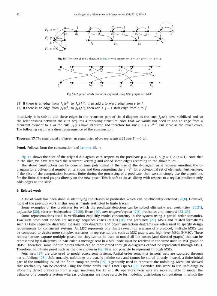
Fig. 15. The slice of the d-diagram in Fig. 6 with respect to (x = 1) ∧ (y = 1) ∧ (z = 1).

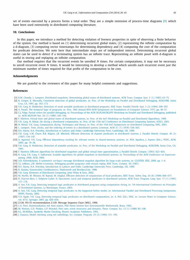
Fig. 16. A poset which cannot be captured using MSC graphs or HMSC.

(1) If there is an edge from J p(e1) to J p( f 1), then add a forward edge from e to f(2) If there is an edge from J p(e1) to J p( f j), then add a j − 1 shift edge from e to f

Intuitively, it is safe to add these edges in the recurrent part of the d-diagram as the cuts J p(ei) have stabilized and sothe relationships between the cuts acquires a repeating structure. Note that we would not need to add an edge from arecurrent element to ⊥ as the cuts J p(ei) have stabilized and therefore for any ei, i � 2, ei−1 can serve as the lower cover.The following result is a direct consequence of the construction.

Theorem 17. The generalized d-diagram as constructed above represents slice(〈E,→〉, p).

Proof. Follows from the construction and Lemma 15. �Fig. 15 shows the slice of the original d-diagram with respect to the predicate p = (x = 1) ∧ (y = 1) ∧ (z = 1). Note that

in the slice, we have removed the recurrent vertex g and added some edges according to the above rules.The above construction can be done in time polynomial in the size of the d-diagram as it requires unrolling the d-

diagram for a polynomial number of iterations and then computing the J p(ei) for a polynomial set of elements. Furthermore,if the slice of the computation becomes finite during the processing of a predicate, then we can simply use the algorithmsfor the finite directed graphs directly on the new poset. This is safe to do as slicing with respect to a regular predicate onlyadds edges to the slice.

9. Related work

A lot of work has been done in identifying the classes of predicates which can be efficiently detected [20,8]. However,most of the previous work in this area is mainly restricted to finite traces.

Some examples of the predicates for which the predicate detection can be solved efficiently are: conjunctive [20,21],disjunctive [20], observer-independent [22,20], linear [20], non-temporal regular [7,8] predicates and temporal [23–25].

Some representations used in verification explicitly model concurrency in the system using a partial order semantics.Two such prominent models are message sequence charts (MSCs) [26] and petri nets [27]. MSCs and related formalismssuch as time sequence diagrams, message flow diagrams, and object interaction diagrams are often used to specify designrequirements for concurrent systems. An MSC represents one (finite) execution scenario of a protocol; multiple MSCs canbe composed to depict more complex scenarios in representations such as MSC graphs and high-level MSCs (HMSC). Theserepresentations capture multiple posets but they cannot be used to model all the posets (and directed graphs) that can berepresented by d-diagrams. In particular, a message sent in a MSC node must be received in the same node in MSC graph orHMSC. Therefore, some infinite posets which can be represented through d-diagrams cannot be represented through MSCs.Therefore, an infinite poset such as the one shown in Fig. 16 is not possible to represent through MSCs.

Petri nets [27] are also used to model concurrent systems. Partial order semantics in petri nets are captured throughnet unfoldings [28]. Unfortunately, unfoldings are usually infinite sets and cannot be stored directly. Instead, a finite initialpart of the unfolding, called the finite complete prefix [29] is generally used to represent the unfolding. McMillan showedthat reachability can be checked using the finite prefix itself. Later Esparza [30] extended this work to use unfoldings toefficiently detect predicates from a logic involving the EF and AG operators. Petri nets are more suitable to model thebehavior of a complete system whereas d-diagrams are more suitable for modeling distributing computations in which the

V.K. Garg et al. / Information and Computation 234 (2014) 26–43 43

set of events executed by a process forms a total order. They are a simple extension of process-time diagrams [9] whichhave been used extensively in distributed computing literature.

10. Conclusions

In this paper, we introduce a method for detecting violation of liveness properties in spite of observing a finite behaviorof the system. Our method is based on (1) determining recurrent global states, (2) representing the infinite computation bya d-diagram, (3) computing vector timestamps for determining dependency and (4) computing the core of the computationfor predicate detection. We note here that intermediate steps are of independent interest. Determining recurrent globalstates can be used to detect if a terminating system has an infinite trace. Representing an infinite poset with d-diagram isuseful in storing and replaying an infinite computation.

Our method requires that the recurrent events be unrolled N times. For certain computations, it may not be necessaryto unroll recurrent event N times. It would be interesting to develop a method which unrolls each recurrent event just theminimum number of times required for that prefix of the computation to be core.

Acknowledgments

We are grateful to the reviewers of this paper for many helpful comments and suggestions.

References

[1] K.M. Chandy, L. Lamport, Distributed snapshots: Determining global states of distributed systems, ACM Trans. Comput. Syst. 3 (1) (1985) 63–75.[2] R. Cooper, K. Marzullo, Consistent detection of global predicates, in: Proc. of the Workshop on Parallel and Distributed Debugging, ACM/ONR, Santa

Cruz, CA, 1991, pp. 163–173.[3] V.K. Garg, B. Waldecker, Detection of weak unstable predicates in distributed programs, IEEE Trans. Parallel Distrib. Syst. 5 (3) (1994) 299–307.[4] A. Pnueli, The temporal logic of programs, in: Proc. 18th Annual IEEE-ACM Symposium on Foundations of Computer Science, 1977, pp. 46–57.[5] C.J. Fidge, Partial orders for parallel debugging, in: Proceedings of the ACM SIGPLAN/SIGOPS Workshop on Parallel and Distributed Debugging, published

in: ACM SIGPLAN Not. 24 (1) (1989) 183–194.[6] F. Mattern, Virtual time and global states of distributed systems, in: Proc. of the Int’l Workshop on Parallel and Distributed Algorithms, 1989.[7] V.K. Garg, N. Mittal, On slicing a distributed computation, in: Proc. of the 15th Int’l Conference on Distributed Computing Systems, ICDCS, 2001.[8] N. Mittal, V.K. Garg, Computation slicing: Techniques and theory, in: Proc. of the 15th Int’l Symposium on Distributed Computing, DISC, 2001.[9] L. Lamport, Time, clocks, and the ordering of events in a distributed system, Commun. ACM 21 (7) (1978) 558–565.

[10] B.A. Davey, H.A. Priestley, Introduction to Lattices and Order, Cambridge University Press, Cambridge, UK, 1990.[11] V.K. Garg, C.M. Chase, R.B. Kilgore, J.R. Mitchell, Efficient detection of channel predicates in distributed systems, J. Parallel Distrib. Comput. 45 (2)

(1997) 134–147.[12] A. Agarwal, V.K. Garg, Efficient dependency tracking for relevant events in shared-memory systems, in: M.K. Aguilera, J. Aspnes (Eds.), PODC, ACM,

2005, pp. 19–28.[13] V.K. Garg, B. Waldecker, Detection of unstable predicates, in: Proc. of the Workshop on Parallel and Distributed Debugging, ACM/ONR, Santa Cruz, CA,

1991.[14] F. Mattern, Efficient algorithms for distributed snapshots and global virtual time approximation, J. Parallel Distrib. Comput. (1993) 423–434.[15] R. Garg, V.K. Garg, Y. Sabharwal, Scalable algorithms for global snapshots in distributed systems, in: Proceedings of the ACM Conference on Supercom-

puting, 2006, ACM, 2006.[16] A.D. Kshemkalyani, A symmetric o(n log n) message distributed snapshot algorithm for large-scale systems, in: CLUSTER, IEEE, 2009, pp. 1–4.[17] T.J. LeBlanc, J.M. Mellor-Crummey, Debugging parallel programs with instant replay, IEEE Trans. Comput. 36 (1987).[18] B.A. Davey, H.A. Priestley, Introduction to Lattices and Order, Cambridge University Press, Cambridge, UK, 1990.[19] R. Stanley, Enumerative Combinatorics, Wadsworth and Brookes/Cole, 1986.[20] V.K. Garg, Elements of Distributed Computing, John Wiley & Sons, 2002.[21] M. Hurfin, M. Mizuno, M. Raynal, M. Singhal, Efficient detection of conjunctions of local predicates, IEEE Trans. Softw. Eng. 24 (8) (1998) 664–677.[22] B. Charron-Bost, C. Delporte-Gallet, H. Fauconnier, Local and temporal predicates in distributed systems, ACM Trans. Program. Lang. Syst. 17 (1) (1995)

157–179.[23] A. Sen, V.K. Garg, Detecting temporal logic predicates in distributed programs using computation slicing, in: 7th International Conference on Principles

of Distributed Systems, La Martinique, France, 2003.[24] A. Sen, V.K. Garg, Detecting temporal logic predicates in the happened before model, in: International Parallel and Distributed Processing Symposium,

IPDPS, Florida, 2002.[25] V.A. Ogale, V.K. Garg, Detecting temporal logic predicates on distributed computations, in: A. Pelc (Ed.), DISC, in: Lecture Notes in Computer Science,

vol. 4731, Springer, 2007, pp. 420–434.[26] Z.120. ITU-TS recommendation Z.120: Message Sequence Chart (MSC), 1996.[27] C.A. Petri, Kommunikation mit Auto-maten, PhD thesis Institut fuer Instrumentelle Mathematik, Bonn, 1962.[28] M. Nielsen, G.D. Plotkin, G.P. Winskel, Petri nets, event structures and domains, Theor. Comput. Sci. 13 (1) (1980) 85–108.[29] K.L. McMillan, Symbolic Model Checking, Kluwer Academic Publishers, 1993.[30] J. Esparza, Model checking using net unfoldings, Sci. Comput. Program. 23 (2) (1994) 151–195.