Modeling and Analysis of a Feedstock Logistics Problem

Jason D. Judd

Dissertation submitted to the faculty of the Virginia Polytechnic Institute and State University in

partial fulfillment of the requirements for the degree of

Doctor of Philosophy

in

Industrial and Systems Engineering

Subhash C. Sarin, Chair

John S. Cundiff, Co-Chair

Douglas R. Bish

C. Patrick Koelling

March 30, 2012

Blacksburg, Virginia

Keywords: multiple asymmetric traveling salesman problem (mATSP), location-allocation, p-

median problem, location-routing problem, Benders’ decomposition, nested Benders’

decomposition, aggregation, bio-crude oil, logistics, transportation, preprocessing, mix integer

programming, supply chain analysis, harvest, storage, transportation, biomass, switchgrass,

supply chain logistics, round bale, square bale, biomass contracts

Copyright 2012, Jason D. Judd

Modeling and Analysis of a Feedstock Logistics Problem

Jason D. Judd

(ABSTRACT)

Recently, there has been a surge in the research and application of “Green energy” in the United

States. This has been driven by the following three objectives: (1) to reduce the nation’s reliance

on foreign oil, (2) to mitigate emission of greenhouse gas, and (3) to create an economic stimulus

within the United States. Switchgrass is the biomass of choice for the Southeastern United

States. In this dissertation, we address a feedstock logistics problem associated with the delivery

of switchgrass for conversion into biofuel. In order to satisfy the continual demand of biomass

at a bioenergy plant, production fields within a 48-km radius of its location are assumed to be

attracted into production. The bioenergy plant is expected to receive as many as 50-400 loads of

biomass per day. As a result, an industrialized transportation system must be introduced as early

as possible in order to remove bottlenecks and reduce the total system cost. Additionally, we

assume locating multiple bioenergy plants within a given region for the production of biofuel.

We develop mixed integer programming formulations for the feedstock logistics problem that we

address and for some related problems, and we solve them either through the use of

decomposition-based methods or directly through the use of CPLEX 12.1.0.

The feedstock logistics problem that we address spans the entire system-from the growing of

switchgrass to the transporting of bio-crude oil, a high energy density intermediate product, to a

refinery for conversion into a final product. To facilitate understanding, we present the reader

with a case study that includes a preliminary cost analysis of areal-life-based instance in order to

provide the reader appropriate insights of the logistics system before applying optimization

techniques for its solution. First, we consider the benefits of active versus passive ownership of

the production fields. This is followed by a discussion on the selection of baler type, and then, a

discussion of contracts between various business entities. The advantages of storing biomass at a

satellite storage location (SSL) and interactions between the operations performed at the

production field with those performed at the storage locations are then established. We also

provide a detailed description of the operations performed at a SSL. Three potential equipment

iii

options are presented for transporting biomass from the SSLs to a utilization point, defined in

this study as a Bio-crude Plant (BcP). The details of the entire logistics chain are presented in

order to highlight the need for making decisions in view of the entire chain rather than basing

them on its segments.

We model the feedstock logistics problem as a combination of a 2-level facility location-

allocation problem and a multiple traveling salesmen problem (mATSP). The 2-level facility

location-allocation problem pertains to the allocation of production fields to SSLs and SSLs to

one of the multiple bioenergy plants. The mATSP arises because of the need for scheduling

unloading operations at the SSLs. To this end, we provide a detailed study of 13 formulations of

the mATSP and their reformulations as ATSPs. First, we assume that the SSLs are always full,

regardless of when they are scheduled to be unloaded. We, then, relax this assumption by

providing precedence constraints on the availability of the SSLs. This precedence is defined in

two different ways and, is then, effectively modeled utilizing all the formulations for the mATSP

and ATSP.

Given the location of a BcP for the conversion of biomass to bio-crude oil, we develop a

feedstock logistics system that relies on the use of SSLs for temporary storage and loading of

round bales. Three equipment systems are considered for handling biomass at the SSLs, and

they are either placed permanently or are mobile, and thereby, travel from one SSL to another.

We use a mathematical programming-based approach to determine SSLs and equipment routes

in order to minimize the total cost incurred. The mathematical program is applied to a real-life

production region in South-central Virginia (Gretna, VA), and it clearly reveals the benefits of

using SSLs as a part of the logistics system. Finally, we provide a sensitivity analysis on the

input parameters that we used. This analysis highlights the key cost factors in the model, and it

emphasizes areas where biggest gains can be achieved for further cost reduction.

For a more general scenario, where multiple BcPs have to be located, we use a nested Benders’

decomposition-based method. First, we prove the validity of using this method. We, then,

employ this method for the solution of a potential real-life instance. Moreover, we successfully

iv

solve problems that are more than an order of magnitude larger than those solved directly by

CPLEX 12.1.0.

Finally, we develop a Benders’ decomposition-based method for the solution of a problem that

gives rise to a binary sub-problem. The difficulty arises because of the sub-problem being an

integer program for which the dual solution is not readily available. Our approach consists of

first solving the integer sub-problem, and then, generating the convex hull at the optimal integer

point. We illustrate this approach for an instance for which such a convex hull is readily

available, but otherwise, it is too expensive to generate for the entire problem. This special

instance is the solution of the mATSP (using Benders’ decomposition) for which each of the sub-

problems is an ATSP. The convex hull for the ATSP is given by the Dantzig, Fulkerson, and

Johnson constraints. These constraints at a given integer solution point are only polynomial in

number. With the inclusion of these constraints, a linear programming solution and its

corresponding dual solution can now be obtained at the optimal integer points. We have proven

the validity of using this method. However, the success of our algorithm is limited because of a

large number of integer problems that must be solved at every iteration. While the algorithm is

theoretically promising, the advantages of the decomposition do not seem to outweigh the

additional cost resulting from solving a larger number of decomposed problems.

This research has been supported by the United States Department of Agriculture under

USDA/CSREES Grant #2008-38420-18742

v

Dedication

To my honey, for making life sweet.

vi

Acknowledgements

Naturally, I would like to begin by thanking my Mom and Dad. They have supported me from

the very beginning in all my endeavors. I am constantly amazed at their parenting skills and

understand why many of my friends looked to them as a second set of parents. Thank you for

giving me the freedom I demanded and the direction I needed so badly.

Additionally, I must thank Mrs. Benson and Mrs. Harris from Parowan High School. I’m sure

that they probably would have scoffed, laughed and sent you away thinking that was a nice joke

if you had told them that their student, a punk teenager with an authority problem, would

someday have spent 8 years in the Marine Corps and upon completing 2 college degrees end up

getting a Masters and Ph. D at a top tier University. However, from them I gained a perception

that I could do much more with my life then I had at first anticipated. I thank them for not just

putting up with me, but trying to steer me onto the right course. From them I gained a desire to

prove to myself and others that I really was worth something. Thank you for putting up with the

mayhem that I may have caused from time to time.

And then there is the late Rigel Freden. I met Rigel (named after a star in the Orion

constellation) when we were both seniors in high school. From Rigel I learned that people really

do read for pleasure and learn because it’s fun. He also taught me that you can be different and

enjoy it. Additionally, he’s probably the smartest person I’ve ever met (I never came across a

word that he didn’t know the definition to, although I spent a lot of time looking words up in a

dictionary to test him.) The day he died was sad, and mourned by many. Since meeting Rigel,

his Dad, Eric, has become much of a second father to me. Eric has a Ph. D in Mathematics and

actively does abstract research that boggles just about anybody’s mind, mine included. Eric has

been a great professional role model for me and has given me a good deal of great advice. Thank

you to you and your family for their friendliness over the years, I look forward to our many

adventures in the future.

And, I must thank Dr. Sarin. I have never met a man that is more thorough or diligent in his

work. I am consistently amazed at his skill to be a silent slave driver. I can think of many nights

vii

that I stayed up far too late because I’d been “hoodwinked” into getting some research done

within a short time frame. Additionally, I thank him for putting up with my terrible English

writing skills and for molding me into a professional. From him I’ve learned how to think

analytically, write technically, and to not cut corners. I would also like to thank Dr. Cundiff for

providing the funding opportunity to perform this research and the many countless hours he

spent teaching me about feedstock logistics. His perspective has been a huge guide in this work.

Without him, this research would have had much less meaning. With him, we’ve been able to

perform research in a domain that is in its infancy. Thank you for all the time and effort you put

into my research even after you have “retired.” (I don’t believe his work load reduced one bit

since retiring.) A warm felt thank you goes out to the other two members of my committee, Dr.

Koelling and Dr. Bish, for their support of me in the research.

Another thank you goes out to my future employer for validating that this entire process was

worth the effort. Additionally, I thank all of my friends I’ve made along the way. I could make

a list, but you know who you are and I would regretfully miss someone if I attempted a list.

Thank you to all of my friends on campus and my friends at church. You’ve made life much

easier and more pleasant as I’ve journeyed through my life in Blacksburg.

And most importantly, I have to thank my wife for her support during this process and for not

openly doubting me when I said that it would be worth the effort. She’s the mother of our

children and the love of my life.

viii

Table of Contents

Chapter 1 Motivation and Background ...................................................................................................... 1

1.1. Motivation .................................................................................................................................... 1

1.2. Background .................................................................................................................................. 2

1.3. Overarching problems ................................................................................................................ 7

1.4. Specific problems addressed ...................................................................................................... 9

1.4.1 Detailed description of feedstock logistics ........................................................................ 9

1.4.2 A feedstock logistics system to serve a bio-crude plant ................................................. 10

1.4.3 A feedstock logistics system to serve a refinery ............................................................. 11

1.4.4 Multiple asymmetric traveling salesmen problem with and without precedence

constraints: performance comparison of various formulations ................................... 12

1.4.5 Benders’ decomposition for problems with an integer sub-problem ................................ 13

Chapter 2 Detailed Description of a Feedstock Logistics System ............................................................ 15

2.1. Introduction ................................................................................................................................ 15

2.2. Contract agreements .................................................................................................................. 16

2.2.1 Stock-out risk at the plant ................................................................................................... 16

2.2.2 Bale delivery compensation ................................................................................................ 17

2.3. Management of harvesting equipment ...................................................................................... 18

2.3.1 Active owner ....................................................................................................................... 19

2.3.2 Passive owner ..................................................................................................................... 19

2.3.3 Crop damage risks ............................................................................................................... 20

2.4. Agricultural versus industrial operations .................................................................................... 21

2.4.1 Field management and harvest windows ........................................................................... 22

2.4.2 Transportation of biomass from a production field to a SSL .............................................. 23

2.5. Baling and storage of Switchgrass .............................................................................................. 24

2.5.1 Bale types for the Piedmont region .................................................................................... 24

2.5.2 Protecting the bale during storage ..................................................................................... 26

2.5.3 Production field owner accountability ................................................................................ 27

2.5.4 Bale quality standards ......................................................................................................... 28

2.5.5 Advantages of storage ........................................................................................................ 29

2.6. SSL equipment options, assumptions, and justification ............................................................. 30

ix

2.6.1 Overview of SSL equipment options ................................................................................... 32

2.6.2 Rear-loading rack option ..................................................................................................... 33

2.6.3 Side-loading rack option ..................................................................................................... 36

2.6.4 Densification option ............................................................................................................ 37

2.6.5 SSL to plant hauling contract .............................................................................................. 38

2.7. Basic transportation equipment needs ...................................................................................... 39

2.7.1 Number of SSL loading operations ...................................................................................... 39

2.7.2 Total number of trucks required ......................................................................................... 40

2.7.3 Total number of racks required .......................................................................................... 41

2.7.4 Total number of trailers required ....................................................................................... 43

2.8. Operations at the bio-crude plant and transportation to the refinery ...................................... 43

2.8.1 Size reduction operations ................................................................................................... 44

2.8.2 Operations at the receiving facility ..................................................................................... 44

2.8.3 Conversion techniques ........................................................................................................ 45

2.8.4 Operations for transportation from the bio-crude plant to the refinery ........................... 47

2.9. Application to a real-life scenario ............................................................................................... 51

2.9.1 GIS database management ................................................................................................. 52

2.9.2 Parameter setting ............................................................................................................... 53

2.9.3 Operation plans for SSLs ..................................................................................................... 55

2.9.4 Parameter setting-for transportation from the bio-crude plant to the refinery ................ 57

2.9.5 A simplified analysis ............................................................................................................ 57

2.10. Summary and concluding remarks.............................................................................................. 58

Chapter 3 Design, Modeling, and Analysis of a Feedstock Logistics System to Serve a Bio-crude Plant. 61

3.1. Description of the biomass logistics system ........................................................................... 61

3.1.1 Transportation of biomass from production fields to satellite storage locations .............. 62

3.1.2 Operations at a satellite storage location ........................................................................... 62

3.1.3 Operations at the receiving facility ..................................................................................... 64

3.2. Problem statement and mathematical formulations of the feedstock logistics problem .... 65

3.3. Results and discussion .............................................................................................................. 72

3.3.1 Additional parameter setting .............................................................................................. 73

3.3.2 Comparison of model formulations .................................................................................... 73

3.3.3 Comparison of equipment systems .................................................................................... 74

x

3.3.4 Comparison of the solutions obtained with a heuristic solution ........................................ 77

3.3.5 Sensitivity analysis .............................................................................................................. 79

3.4. Concluding remarks .................................................................................................................. 80

Chapter 4 Design, Model, and Analysis of a Feedstock Logistics System to Serve a Refinery ................. 81

4.1. Introduction ................................................................................................................................. 81

4.2. Biomass logistics system ............................................................................................................ 82

4.3. Problem definition, literature review, and model formulation .................................................... 85

4.4. Solution methodology via nested Benders’ decomposition ....................................................... 91

4.5. Application to a potential real-life scenario .............................................................................. 100

4.6. Concluding remarks .................................................................................................................. 103

Chapter 5 Multiple Asymmetric Traveling Salesmen Problem with and without Precedence Constraints:

Performance Comparison of Various Formulations .............................................................. 105

5.1. Introduction ............................................................................................................................. 105

5.2. Problem overview ..................................................................................................................... 106

5.3. Formulations for the multiple asymmetric traveling salesmen problem ................................. 107

5.3.1 Formulations with SECs based on the ranking of cities .................................................... 107

5.3.2 Formulations with SECs based on multi-commodity flows............................................... 112

5.3.3 Transformation of mATSP to an equivalent ATSP ............................................................. 118

5.4. Computational comparison of various mATSP formulations .................................................... 125

5.5. mATSP formulations with special precedence constraints ....................................................... 130

5.5.1 Formulations for PCmATSP ............................................................................................... 130

5.5.2 Transformation of PCmATSP to an equivalent PCATSP .................................................... 133

5.5.3 Computational comparison of various PCmATSP and PCATSP formulations ................... 134

5.6. mATSP formulations with general precedence constraints...................................................... 139

5.6.1 Formulations for G-PCmATSP ........................................................................................... 140

5.6.2 Transformation of G-PCmATSP to an equivalent G-PCATSP ............................................. 144

5.6.3 Computational comparison of various G-PCmATSP and G-PCATSP formulations ............ 146

5.7. Summary and concluding remarks............................................................................................ 150

Chapter 6 Benders’ Decomposition for Problems with an Integer Sub-problem .................................. 152

6.1. Introduction ............................................................................................................................. 152

6.2. Literature review on decomposition techniques .................................................................. 153

6.2.1 Column generation .......................................................................................................... 153

xi

6.2.2 Lagrangian relaxation ........................................................................................................ 155

6.2.3 Benders’ decomposition ................................................................................................... 156

6.2.4 Combined decomposition techniques .............................................................................. 160

6.2.5 Acceleration techniques ................................................................................................... 160

6.3. Benders’ decomposition for integer sub-problems .............................................................. 160

6.4. Benders’ decomposition for integer sub-problems-a special case ........................................... 164

6.5. Model presentation, empirical investigation, and results ........................................................ 166

6.5.1 MTZ non-decomposed model ........................................................................................... 167

6.5.2 FL2 non-decomposed model............................................................................................. 169

6.5.3 Proposed algorithm for MTZ and FL2 ............................................................................... 170

6.5.4 Empirical investigation and results ................................................................................... 172

6.6. Concluding remarks ................................................................................................................ 177

Chapter 7 Concluding Remarks and Directions for Future Research ..................................................... 178

References . ........................................................................................................................................... 181

xii

List of Figures

Figure 1.1: An aerial depiction of production fields ....................................................................... 3 Figure 1.2: An aerial depiction of production fields and the potential satellite storage locations .. 5

Figure 1.3: Graphical interpretation of two equipment options ...................................................... 5 Figure 1.4: A simplified feedstock logistics system overview ....................................................... 6 Figure 2.1: Grapple loader used for rack loading at a SSL. .......................................................... 34 Figure 2.2: Rack loader used for rack loading for the Rear-loading rack option. ........................ 35 Figure 2.3: Concept for side-loading of bales into the rack on the trailer .................................... 37

Figure 2.4: Aerial view of the three SSL equipment options ....................................................... 39 Figure 2.5: Aerial view of the two refinery models ...................................................................... 48 Figure 3.1: Graphical depiction for the 48-km database using permanent equipment option ...... 76

Figure 3.2: Graphical depiction for the 32-km Resop solutions ................................................... 78 Figure 4.1: Sample area of production fields and potential satellite storage locations (SSLs) .... 83 Figure 4.2: Potential Bio-crude plant region in Virginia and North Carolina ............................ 101

Figure 5.1: An ATSP solution for the mATSP problem with ......................................... 119 Figure 5.2: Comparison of the required CPU times (log-scale) without precedence ................. 129

Figure 5.3: Comparison of LP relaxations (% optimality gaps) without precedence ................. 129 Figure 5.4: Comparison of the required CPU times with precedence ........................................ 138

Figure 5.5: Comparison of LP relaxations (% optimality gaps) with precedence ...................... 138 Figure 5.6: Comparison of the required CPU times with general precedence ............................ 149 Figure 5.7: Comparison of LP relaxations (% optimality gaps) with general precedence ......... 149

Figure 6.1: Proposed algorithm to obtain dual solution for integer sub-problem ....................... 162 Figure 6.2: Graphical representation of the LP relaxation and convex hull ............................... 163

Figure 6.3: A graphical example of two sets that result in tight DFJ constraints ....................... 165 Figure 6.4: Upper and lower bounds for the ftv35 m = 2 data set .............................................. 176

xiii

List of Tables

Table 2.1: Equipment options at a SSL ........................................................................................ 34

Table 2.2: Equipment specifications for the grinding operations ................................................. 45 Table 2.3: Cost analysis for the rail car loading facilities at a bio-crude plant ............................. 49 Table 2.4: Equipment specifications for operations at the SSL .................................................... 55 Table 2.5: Overview of results for transportation from the SSL to the bio-crude plant ............... 57 Table 2.6: Trucking variable and fixed transportation cost parameters........................................ 58

Table 2.7: Rail variable and fixed transportation cost parameters ................................................ 58 Table 2.8: Total cost from the production field to the bio-crude plant ......................................... 58 Table 3.1: Comparison of model formulations ............................................................................. 74 Table 3.2: Comparison of equipment systems .............................................................................. 75

Table 3.3: Comparison of heuristic and optimal solutions ........................................................... 77 Table 3.4: Sensitivity analysis of cost parameters ........................................................................ 80

Table 4.1: Equipment specifications for operations performed at a satellite storage location ..... 84 Table 4.2: Cost analysis for loading at a bio-crude plant ............................................................. 85

Table 4.3: Size of datasets used for analysis............................................................................... 103 Table 4.4: Potential real-life scenario solution results ................................................................ 104 Table 5.1: Comparison of the mATSP models ........................................................................... 126

Table 5.2: Comparison of the ATSP models .............................................................................. 127 Table 5.3: Comparison of the PCmATSP models ...................................................................... 136

Table 5.4: Comparison of the PCATSP models ......................................................................... 137 Table 5.5: Comparison of the G-PCmATSP models .................................................................. 147 Table 5.6: Comparison of the G-PCATSP models ..................................................................... 148

Table 6.1: Empirical investigation using the TSP data ............................................................... 174

Table 6.2: Empirical investigation using random data ............................................................... 175 Table 6.3: No. of iterations, bounds, and optimality gap for the ftv35 m = 2 24 hour run ......... 177

Chapter 1 Motivation and Background Table 1: Hidden table

1.1. Motivation Over the course of the last 20 years, cellulosic biofuels have become an environmentally

attractive and technologically feasible liquid fuel alternative to fossil fuels. To make this

alternative economically viable, it is essential to judiciously design the underlying logistics

system.

Fuels from renewable resources are being developed as a means to reduce the impact of

greenhouse gases (emissions from the use of fossil fuels) on the environment, and, perhaps more

importantly, to reduce the U.S. dependence on imported oil. Many studies have demonstrated

the availability of biomass for conversion into energy [34, 62, 111]. However, to garner this

source of energy, as much as 35-60% of the total cost of cellulosic ethanol at the retail pump

results from the feedstock transportation cost [40]. Therefore, it is essential to reduce this cost as

much as possible in order to make biofuel a viable alternative to petroleum.

The United States government for the last over ten years has provided major funding for the

production of liquid fuels from renewable resources. The main drivers for this development are:

(1) reduction in dependence on imported oil, (2) concern about global climate change resulting

from the release of fossilized carbon into the atmosphere, and (3) a desire to stimulate rural

economies.

First generation renewal fuels are typically defined as fuels that are produced by fermentation of

sugar to produce an alcohol. Ethanol, currently used as a fuel additive (extender) for gasoline, is

an important commercial example. (Ethanol can be described as a “drop-in fuel”, meaning that it

is a fuel-form that can be used with the current fleet of United States automobiles without any

engine modifications.) Second generation drop-in fuels are produced by breaking down the fiber

in biomass to ultimately yield a fuel that can be blended with petroleum fuel. Biomass used for

second generation fuels do not compete directly with the food market. Any lignocellulosic

2

material, woody or herbaceous, can be used as a feedstock for second generation fuels.

Technology to convert lignocellulose materials is not currently available at a commercial scale,

although successful lab scale studies are abundant and a few pilot plants are currently in

operation or under construction. Our focus in this dissertation is bio-crude, a second generation

(liquid) product produced by converting biomass with some version of a fast pyrolysis process. It

is an intermediate energy form that is subsequently refined into a liquid fuel that replaces

petroleum fuel. Third generation fuels are produced from algae growth and have a very different

logistics design from the first and second generation fuels.

In this dissertation, we study the factors effecting the production of second generation fuels with

a focus on switchgrass production in the Southeastern United States (Piedmont region). Our

analysis is generic in nature and can be applied to other feedstocks produced in other regions of

the country. Also, all results are directly applicable to the logistics required to deliver biomass

for direct combustion to produce heat and power.

For this study of the feedstock logistics problem, we focus on the transport of biomass in bale

form from a production field to delivery at a bio-energy plant. After conversion of the raw

biomass into bio-crude oil, we consider the transportation of the oil from a bio-crude plant (BcP)

to a refinery. In the subsequent sections, we provide a general overview to the problem. In

Chapter 2 the details of the feedstock logistics problem are set forth.

1.2. Background

The Piedmont, a physiographic region that covers over one-third of the land area of Virginia, has

potential for attracting a large number of landowners into feedstock production for bio-crude oil.

Much of the Piedmont is characterized by marginal soil which cannot be profitably farmed for

grain production. Additionally, many Piedmont production field owners have produced tobacco

for the cigarette industry. The tobacco market has declined, and these owners need an alternative

crop in order to be economically stable. These production field owners could benefit from the

introduction of a bioenergy industry. Specifically, the concept for this dissertation presumes that

native warm-season grasses will be grown as a feedstock for a series of bio-crude plants.

Switchgrass is chosen as the model species, and hereafter, the term “switchgrass” is used as a

3

generic term for any warm-season grass species that might emerge as a viable feedstock in the

future.

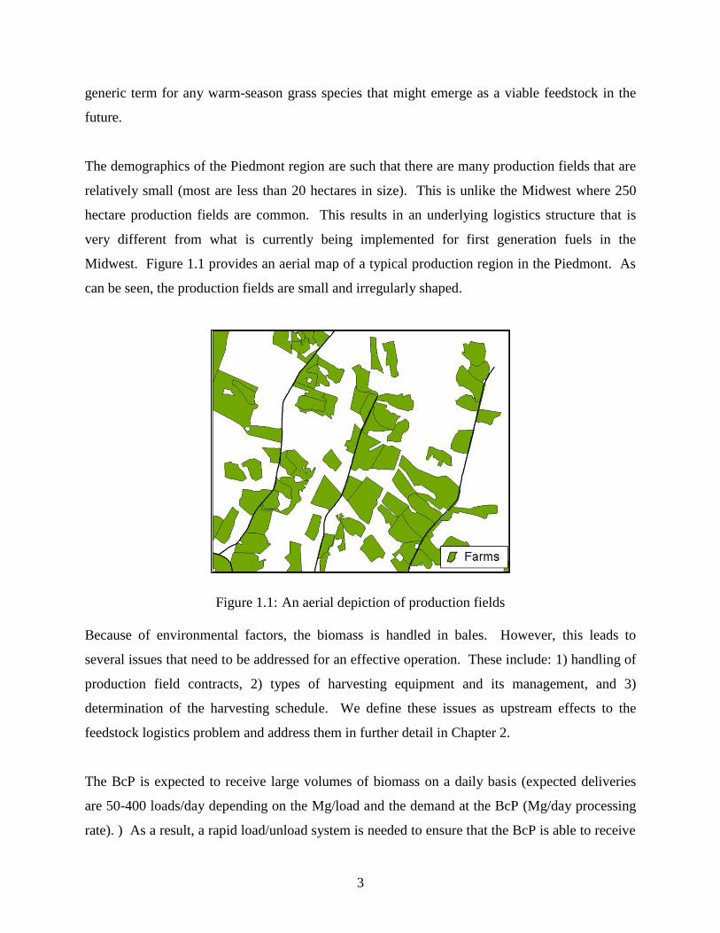
The demographics of the Piedmont region are such that there are many production fields that are

relatively small (most are less than 20 hectares in size). This is unlike the Midwest where 250

hectare production fields are common. This results in an underlying logistics structure that is

very different from what is currently being implemented for first generation fuels in the

Midwest. Figure 1.1 provides an aerial map of a typical production region in the Piedmont. As

can be seen, the production fields are small and irregularly shaped.

Figure 1.1: An aerial depiction of production fields

Because of environmental factors, the biomass is handled in bales. However, this leads to

several issues that need to be addressed for an effective operation. These include: 1) handling of

production field contracts, 2) types of harvesting equipment and its management, and 3)

determination of the harvesting schedule. We define these issues as upstream effects to the

feedstock logistics problem and address them in further detail in Chapter 2.

The BcP is expected to receive large volumes of biomass on a daily basis (expected deliveries

are 50-400 loads/day depending on the Mg/load and the demand at the BcP (Mg/day processing

rate). ) As a result, a rapid load/unload system is needed to ensure that the BcP is able to receive

4

a requisite amount of biomass. Additionally, the equipment that is designed to handle in-field

operations is typically inefficient for transporting biomass on the highway. This is

predominantly a factor of slow transportation speeds, high equipment costs, and loads that do not

approach the maximum gross weight limits in the United States. This demands the use of an

industrialized hauling system for the transportation of biomass as early as possible in the

logistics chain to increase efficiency (Mg/day hauled) and reduce cost ($/Mg).

Satellite storage locations (SSLs) are utilized to implement an industrial operation early in the

logistics chain. These SSLs operate much like a co-op system, where the production fields

within a given sector share a single storage location. The SSLs also provide enough biomass in

one location to justify the use of specialized loading equipment (industrial operations) and

improve system efficiency. A potential SSL is selected from the list of production fields that

meet some basic requirements, which are discussed in further detail in Chapters 2 and 3.)

Clearly, it is not practical to have every production field be selected as a SSL.

Figure 1.2 provides an aerial map of a section of land near Gretna, VA. This figure provides

some intuition as to what the current dataset looks like in terms of the distribution of production

fields and the percentage of production fields that are selected as SSLs.

Once the SSLs have been selected, specialized loading equipment and an industrialized

transportation system are used to transport biomass from the SSLs to the BcP. Once an

equipment option has been selected, it may be stationed permanently at a single SSL for year-

round operation, or it can be designed so that it can be moved from one SSL to the next (see

Figure 1.3). The mobile equipment allows for the size of the SSLs to be greatly reduced while

still fully utilizing the capacity of the equipment. The optimal routing of multiple sets of

equipment results in a multiple traveling salesmen problem (mATSP).

5

Figure 1.2: An aerial depiction of production fields and the potential satellite storage locations

Figure 1.3: Graphical interpretation of two equipment options

6

Once at a BcP, the biomass is reduced in size and then converted into a relatively high energy

intermediate product, the bio-crude oil. The size of the material that is needed as an input to the

BcP is dependent on the type of the conversion process used at the plant. For example, different

processes have specifications of 2 mm, 2 cm, or 10 cm particle lengths. The particle size

specification has some effect on the logistics decisions and this specification is included as a

downstream effect.

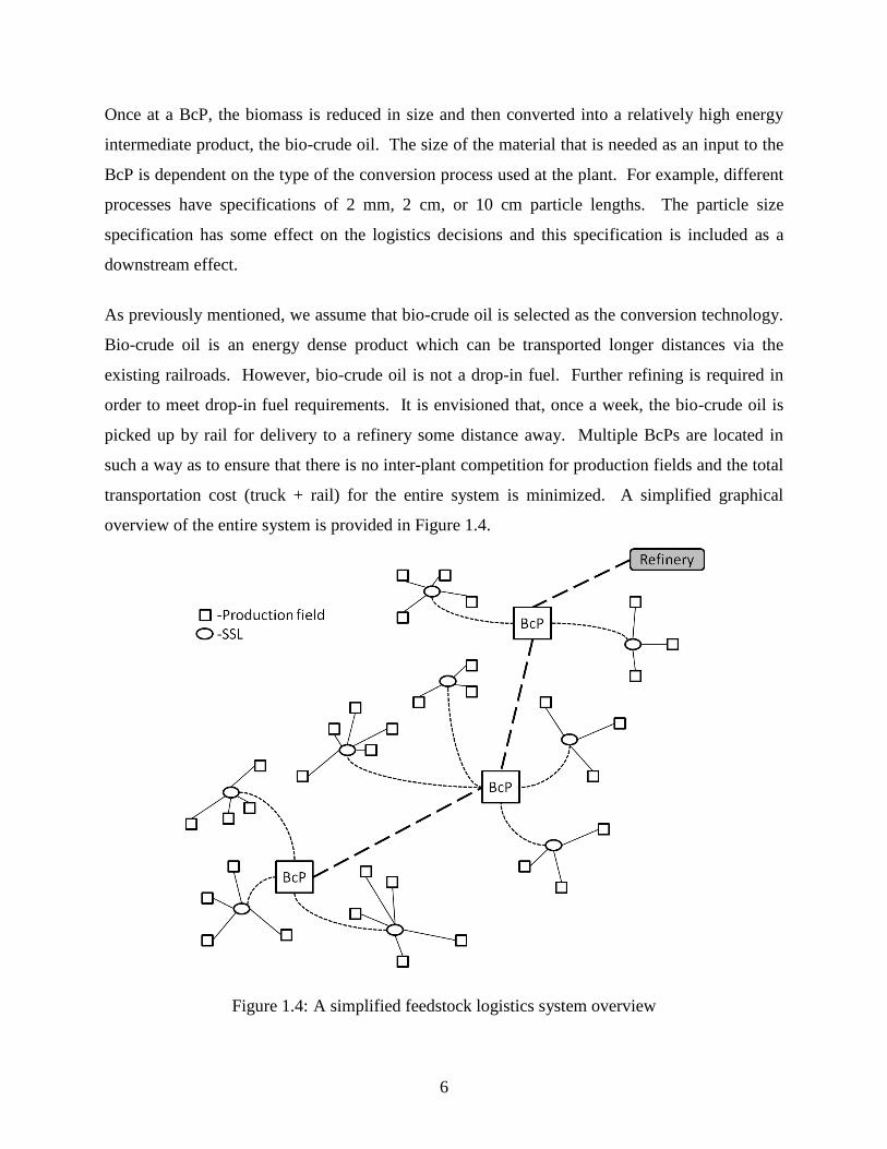
As previously mentioned, we assume that bio-crude oil is selected as the conversion technology.

Bio-crude oil is an energy dense product which can be transported longer distances via the

existing railroads. However, bio-crude oil is not a drop-in fuel. Further refining is required in

order to meet drop-in fuel requirements. It is envisioned that, once a week, the bio-crude oil is

picked up by rail for delivery to a refinery some distance away. Multiple BcPs are located in

such a way as to ensure that there is no inter-plant competition for production fields and the total

transportation cost (truck + rail) for the entire system is minimized. A simplified graphical

overview of the entire system is provided in Figure 1.4.

Figure 1.4: A simplified feedstock logistics system overview

7

1.3. Overarching problems

The feedstock logistics problem that we have introduced above is complex and has many

different aspects that must be addressed in order to optimize the entire system. Herein, we

provide a brief overview of the problem statement, research objectives, and the significant

contributions of the dissertation research.

Statement of overall problem:

The biomass logistics problem (BLP) that we address in this research can be stated as follows:

Given f potential production fields and a set of n potential SSLs, determine the optimal number

of production fields and SSLs, the SSLs placement (production fields on which to build the

satellite storage facilities), and the allocation of production fields to SSLs. Additionally,

determine the optimal locations of the BcPs from a set of predetermined locations so as to

minimize the total cost incurred for: transporting (1) biomass from each production field to a

SSL, (2) biomass to the BcP, and (3) bio-crude oil from the BcP to the refinery, and determine

the minimal-cost routing of the loading equipment among the SSLs.

As described briefly above, each SSL must be visited by the loading equipment. This equipment

routing problem is similar to the multiple asymmetric traveling salesmen problem (mATSP),

which can be stated as follows: Given a set of n potential SSLs (cities) and m equipment sets

(traveling salesmen), determine at most m tours such that, starting from a reference (base) SSL

facility, each equipment set visits a subset of the SSLs and returns to the base SSL facility, and

each selected SSL is visited by exactly one equipment set, for the objective of minimizing the total

distance traveled by all the equipment sets. The ATSP problem has been addressed extensively

over the years in the literature by Laporte [85] and also by Oncan et al. [108]. Work on the

multiple traveling salesmen has been described by Bektas [7], Laporte and Norbert [86], and

Sarin et al. [121].

We address the overall problem introduced above as follows: (1) First, we present, in Chapter 2,

a detailed description of the elements of the feedstock logistics system, which sets the stage for

our analysis in other chapters. (2) Then, in Chapter 3, we address the feedstock logistics problem

to serve a BcP. A mathematical programming-based approach is developed to obtain a minimum

8

cost solution that specifies locations of SSLs, assignment of production fields to SSLs, and

routing of equipment to unload SSLs. We also illustrate the effectiveness of this approach by

applying it to a potential real-life production region near Gretna, in South-central Virginia. (3)

We extend this model in Chapter 4, to develop a feedstock logistics system to serve a refinery,

which now involves location of multiple BcPs and the allocation of SSLs to BcPs along with the

decisions considered in (1). We also apply our approach to a real-life size-based production

region. (4) As routing of multiple sets of unloading equipment among the SSLs is an important

feature of our problem, we address this problem (called multiple ATSP) separately. We address

this problem from two perspectives. First, in Chapter 5, we provide various model formulations

of this problem and present a detailed analysis of their computational effectiveness. Second,

because of the importance of this problem in practice, we investigate, in Chapter 6, a new

solution method for this problem. Our motivation for this investigation is the solution of the

integer sub-problem that arises in the Benders decomposition approach for this case. We present

a novel method to this end, provide its theoretical justification, and also analyze results of a

computational investigation on its performance.

Research objectives

Our overall objective is to mathematically model, design, and analyze a feedstock logistics

system in order to minimize total system cost. To that end, our specific objectives are to:

1. Understand system details: costs, types of equipment, and upstream/downstream issues.

2. Determine location/size/number of SSLs for supplying biomass to a given BcP.

3. Determine locations of BcPs given the location of a refinery.

4. Model equipment travel as a mATSP with and without precedence.

5. Decomposition methods for solving the overall feedstock logistic problem, and

specifically, for solving the mATSP.

Contributions of dissertation research

Our analysis provides the following results/contributions:

1. Better cost estimates for the entire feedstock logistics system.

2. A logistics system that introduces an industrialized system as early in the logistic chain as

is economically feasible.

9

3. Develop mathematical models that effectively capture the desired features of the

feedstock logistics problem.

4. Develop new decomposition-based algorithms that are robust in solving a variety of

problems.

5. New and modified models for the mATSP, a computational investigation of their

performance, and a novel method for solving the mATSP.

1.4. Specific problems addressed

1.4.1 Detailed description of feedstock logistics

The biomass logistics problem (BLP) concerns operations for transporting baled biomass from

the production fields to the SSLs, and then, to the BcPs, and for transporting bio-crude oil from

the BcP to the refinery for conversion into a drop-in fuel. This application is discussed in detail

in Chapter 2, and it serves as a test bed to apply the solution methodologies developed in

subsequent chapters. We address the upstream and downstream effects that play a key role in the

development of a proper logistics system.

The evolution of the logistics chain chosen for analysis is presented via a discussion of the

significant issues that drive the system. We consider the resulting effects of contract agreements,

active versus passive land ownership, baling options, storage, and ownership accountability.

This is followed by a detailed description of three equipment options considered for load-haul

operations to deliver feedstock from the SSLs to the BcP. These topics are addressed to better

understand the factors affecting the logistics system.

The downstream effects are dictated by the conversion process that takes place at the conversion

facility. Multiple types of conversions may be considered within the same logistics system.

However, we assume that the biomass is converted into bio-crude oil, which, while not a drop-in

fuel, is energy rich enough to justify the long haul distances for further refinement into a drop-in

fuel at a refinery. Once conversion takes place at the refinery, the drop-in fuel is transported and

handled within the existing petroleum fuel logistics infrastructure.

10

The principal contributions from the analysis in Chapter 2 are threefold. Foremost, a detailed

description of the feedstock logistics problem is presented. This description leaves the reader

with a stronger understanding of the underlying problems and difficulties associated with the

logistics operations. Second, the effects from decisions outside the feedstock logistics system

are established. These upstream and downstream decisions can have a significant impact on the

solution to the problem. Third, a detailed cost analysis of the system is provided. The costing of

the system is non-trivial, and, from the associated cost, a rudimentary set of results is presented.

The cost parameters established in Chapter 2 are utilized in subsequent chapters as the input

parameters to the respective models.

1.4.2 A feedstock logistics system to serve a bio-crude plant

In Chapter 3, a logistics system that relies on SSLs for temporary storage and loading of round

bales is proposed. We assume that the location of a bio-energy plant for the conversion of

biomass to bio-energy is given. The logistics associated with transporting the biomass from

production fields to the bio-energy plant constitutes a nontrivial task. Hence, in Chapter 3, a

mathematical programming-based approach is utilized to determine SSL placements that

minimize the total cost of: (1) transporting the biomass, (2) utilizing the equipment, and (3)

developing the SSLs. The mathematical program is applied to a real-life production region in

South-central Virginia (Gretna, VA), and it clearly reveals the benefits of using SSLs as a part of

the logistics system.

The three equipment systems for handling biomass at the SSLs that were presented in Chapter 2

are compared using their individual results from the mathematical program. The equipment is

envisioned to be either permanently placed at the SSLs or is mobile, and thereby, travels from

one SSL to another. Two of these equipment systems use racks, similar to a 6.1 m (20 ft.) ISO-

container, for transporting biomass to the bio-energy plant, and are called the Rear-loading Rack

System and Side-loading Rack System. The third system densifies the biomass before

transporting it to the bio-energy plant and is called the Densification System. The results

obtained are also compared with a heuristic solution from the study published by Resop et al.

[118]. Finally, upon completion of the analysis of these systems, the best system is further

studied by applying a sensitivity analysis on the input parameters that were used. This analysis

11

highlights the key cost factors in the model and emphasizes where the biggest gains are

potentially possible for further cost reductions.

The principal contributions of the analysis of a feedstock logistics problem, as it has been

defined, are threefold. First, we present mathematical formulations for the feedstock logistics

problem. This formulation captures the interdependence of the selection of SSLs based on

production field locations, the BcP location, and other SSLs locations. Additionally, these

models provide a framework for comparison with the heuristic solutions presented in the

literature as well as in establishing best practices for application. Second, the results from the

comparison of equipment options and permanent versus mobile equipment provide valuable

information for the implementation of a real-life system. This research emphasizes the

significant additional cost attributed to both the densification system and permanent equipment at

each SSL. Third, the results of the sensitivity analysis help identify areas where potential gains

may be achievable.

1.4.3 A feedstock logistics system to serve a refinery

In Chapter 4, we extend the biomass logistics system of Chapter 3 to include the placement of

multiple BcPs that supply bio-crude oil to a single refinery. The key elements of a biomass

logistics system include the hauling of biomass from the production fields to SSLs (for

densification and industrialized loading), transportation of biomass from the SSLs to BcPs (for

conversion into bio-crude oil), and finally, transportation of the bio-crude oil from the BcPs to a

single refinery (for conversion into a drop-in fuel).

We have developed necessary mathematical models to capture the various design issues involved

for this problem. These include: (1) locating the SSLs and BcPs, (2) allocating production fields

to SSLs and SSLs to BcPs, and (3) scheduling the sequential unloading of SSLs using multiple

sets of equipment. For the implementation of these models, the real cost estimates presented in

Chapter 2 are utilized. However, no real-life dataset is available that is large enough for this

study, and hence, randomly generated datasets are utilized. These randomly generated datasets

are developed to emulate the Piedmont region for the establishment of five BcPs within a 300 x

12

120-km region spanning from Bedford, VA to Robbins, NC and the dataset for the Gretna, VA

area that is introduced in Chapter 3.

A nested Benders’ decomposition-based methodology is then implemented that enables solution

of these real-life-sized problems. Its importance in making effective decisions for the biomass

logistics system is demonstrated. As a result of decomposition, we are able to solve problems

that are more than 25 times as large in number of variables and more than 5 times as large in

number of production fields and SSLs than those solvable via the direct use of CPLEX 12.1.0.

The principal contributions of this study are twofold. First, the mathematical models have been

further expanded to address the selection of BcPs within a very general framework. Second, a

formal proof of nested Benders’ decomposition is provided, and the success of this method is

clearly demonstrated. To the best of our knowledge, this is the first application of nested

Benders’ decomposition to a deterministic problem.

1.4.4 Multiple asymmetric traveling salesmen problem with and without

precedence constraints: performance comparison of various formulations

Biomass is transported from the production fields to a SSL that is within their close proximity.

The SSL provides a central location for the local production field owners to store their biomass

while accruing a minimal cost for transport to the SSL. Once the SSLs have been filled, they are

unloaded using specialized loading equipment. These equipment sets are mobile, thereby

allowing them to move from one SSL to another, which justifies the development of many small

SSLs. Additionally, there are multiple equipment sets that unload the SSLs independently of one

another. The scheduling of the equipment sets among the SSLs results in a mATSP.

The assumption that all the SSLs are full is then relaxed by assuming that certain SSLs must be

unloaded before other SSLs on the same tour. This results in an mATSP with special precedence

(PCmATSP). For this case, it is assumed that the BcP has dictated to the production field

owners a harvest schedule for them to adhere to. The cost associated with having to shut down

the BcP is anticipated to be fairly high, and hence, is alleviated via the SSL precedence. This

special precedence is applied by requiring one SSL to precede another if they are on the same

13

tour. This special precedence is then generalized and designated as G-PCmATSP. The

generalized precedence requires some SSLs to be unloaded prior to other SSLs regardless of

which tours they are assigned to.

In Chapter 5, the mATSP is studied using 13 different formulations that are either new, directly

from the literature, or are modified generalizations of the ATSP. The objective is to study the

effectiveness of these formulations for the mATSP in terms of the CPU time required to generate

an optimal solution by direct application of CPLEX, the tightness of the LP relaxation of the

formulations, among other measures. Furthermore, each of the mATSP formulations is

transformed into an equivalent ATSP formulation. These transformed formulations, are then,

compared with their mATSP formulations counterparts. Finally, a study is performed for the

special and general precedence context discussed above (mATSP, PCmATSP, G-PCmATSP) in

a similar manner.

The principal contributions of the mATSP research in this dissertation are threefold. First, new

models are suggested for the mATSP. Second, a comparative and exhaustive empirical

performance analysis is provided for the mATSP formulations, which reveals each formulation’s

respective strengths and weaknesses and enables a modeler to select an appropriate formulation

to use. Third, the establishment of the precedence relationships for the special and general case

allows for further flexibility when developing a formulation. These precedence relationships are

common in many applications, including the biomass logistics problem (BLP) that is addressed

in this dissertation. The precedence-constrained mATSP formulations that we present are new

and have not been presented in the literature.

1.4.5 Benders’ decomposition for problems with an integer sub-problem

The formulation of a potential real-life problem for the BLP may consist of millions of variables

depending on the type of model used and the extent of data reduction techniques applied. The

decisions involved pertain to where to place the BcPs and how to allocate SSLs and production

fields. An additional decision pertains to the routing of a set of multiple equipment among the

SSLs. In Chapter 4, a formulation for selecting BcPs is presented and a methodology is

developed for its solution. It is applied to the data obtained for Piedmont region. It is likely that

14

several BcPs could potentially be located within this region. The order of anticipated number of

production fields needed per BcP is in thousands and the number of SSLs per BcP is in hundreds

for this data. The resulting formulation is rather large, consisting of millions of binary variables,

and is too large to be solvable on a single computer. We exploit the inherent structure of the

problem and a Benders’ decomposition-based methodology for its solution. This structure

enables solution of the sub-problem as m independent ATSPs, which are much easier to solve

than the initial mATSP.

We provide brief review of several decomposition techniques and justification for the use of

Benders’ decomposition. Following this review, Chapter 6 proposes the use of a novel cutting

plane concept to further tighten the LP relaxation of the sub-problem to obtain nearly integer

optimal solutions. We discuss its implementation for the solution of the mATSP for which the

convex hull of the sub-problem is well-known, but too expensive to generate for the entire

problem. For this case, the problem is solved to optimality to obtain an integer solution of the

sub-problem, and the linear program solution and its corresponding dual solutions are obtained

by adding a polynomial number of constraints that form the convex hull at that point. A set of

problem instances is used to experimentally investigate the effectiveness of these Benders’

decomposition-based techniques and the results of a comparative analysis are presented.

15

Chapter 2 Detailed Description of a Feedstock Logistics System

2. Hidden figure

Table 2: Hidden table

2.1. Introduction

In the Piedmont (South-central Virginia), switchgrass has been selected as the biomass of choice

for its drought tolerance and relatively high yields on marginal soils. In this chapter, a study of

the interactions between production field operations and logistic operations is set forth. The

purpose of this chapter is to clearly present a discussion of some of the interacting issues that

occur between production field operations and logistics operations. Production field operations

are defined as the production, harvesting, local transport, and storage of switchgrass within a

local region. The logistics system covers all operations starting from the storage of switchgrass

until its delivery in size-reduced form for processing at a BcP.

We address a feedstock logistics problem that spans the entire system-from the growing of

switchgrass to the transporting of bio-crude oil, a high energy density intermediate, to a refinery

for conversion into a final product. To facilitate understanding, we provide the reader with a

case study that includes a preliminary cost analysis. The purpose of this cost analysis is to

provide the reader appropriate insights of the logistics system before the application of

optimization techniques in later chapters. First, we consider the benefits of active versus passive

ownership of the production fields. This is followed by a discussion on the selection of baler

type, and then, a discussion of contracts between the various business entities. The advantages

of storage at a satellite storage location (SSL), and interactions between operations at the

production field with these storage locations are then established. Following these remarks,

detailed descriptions of operations at a SSL are presented. Three potential equipment options are

considered for transporting biomass from the SSLs to a utilization point, defined in this study as

a BcP. At the BcP, the raw biomass is converted into an intermediate liquid (bio-crude oil), and

then transported to a refinery. The concept chosen for this study assumes that there will be

multiple BcPs located within the Piedmont region that collectively produce bio-crude oil for

transport to a single refinery for conversion into a “drop-in fuel”. A drop-in fuel is defined as a

16

liquid fuel which can be used interchangeably with a petroleum fuel. The details of the entire

logistics chain are presented, and we establish the need for decisions to be based on the entire

logistics chain instead of making decisions to optimize a given segment of the chain.

Although many of the issues and problems discussed in this chapter are general in nature, some

are problem-specific to the Piedmont. Switchgrass is used as the model biomass species. The

mode of transportation is limited to truck and rail transportation, since these two transportation

methods are the most common means to deliver biomass over distances less than 160 km [139].

We perform a detailed cost analysis of the operations pertaining to a general biomass logistics

problem and illustrate it using a specific case study. A key issue is the balancing of the total cost

incurred for transporting raw biomass, a bulky low-value product, from the production fields to

the BcPs, and the total cost incurred for transporting bio-crude oil, a higher-value more energy

dense product, from the plants to the refinery. We consider the use of an existing rail network

for the delivery of bio-crude oil to the refinery.

2.2. Contract agreements

As stated in the previous section, the design of the logistics system depends on the business

relationship between the various parties. These business relationships are generally set forth in

contracts. Basically, the contracts define who will do what operations on what time schedule.

Each business entity would want to minimize the risk that they undertake.

2.2.1 Stock-out risk at the plant

The capital cost associated with the building of a full scale conversion facility is significant.

Searcy and Flynn [124] perform a detailed cost analysis of several types of conversion facilities.

In order to fully utilize the economies of scale, these conversion facilities may be quite large,

Sokhansanj et al. [139] suggest 2000-5000 Mg of feedstock per day. However, for the

implementation of our feedstock logistics model utilizing BcPs, the economy of scale benefits

are expected to come into effect at a much smaller size. The BcPs emulate the Advanced

Regional Biomass Processing Depots (ARBPD) suggested by Eranki et al. [37]. These ARBPDs

are a central location that requires a relatively high capital investment and provide potential to

17

mix several conversion technologies at a single location. These technologies may include leaf

protein concentrate, leaf/stem separation, pyrolysis into bio-crude oil, and anaerobic digestion.

For simplicity, we envision that the only conversion taking place is the conversion of biomass

into bio-crude oil. Utilizing multiple smaller BcPs helps to limit the transportation cost and

reduce the stock-out risk at the refinery.

For the establishment of a BcP, there must exist sufficient evidence for the owners/lenders to

believe that the BcP will indeed be successful. Lenders will determine the interest rate to charge

in order to properly compensate for their assumed risk. To this end, the establishment of

contracts with potential switchgrass production field owners are essential to mitigate the total

risk incurred.

The use of a contract for the purchase of feedstock is of utmost importance to ensure that the

BcP’s, and the production field owner’s, risk are both minimized. The BcP is at risk for not

having enough switchgrass to provide continuous operation. Continuous operation is desired due

to high startup and shutdown costs at the plant. For this reason, it is in the BcPs best interest to

sign long-term contracts (10-15 years, equivalent to the average life of a stand of switchgrass

before reseeding) to ensure that the production field owners provide the switchgrass as promised.

Contracts this long are a new paradigm for agriculture in the Southeast, which has typically

operated on a “spot market” model.

The production field owner has an interest in a contract to ensure that a fair market value price is

offered. The BcP may be viewed as a monopoly because there are no other significant markets

for switchgrass. For this reason, the production field owner will want to lock in a purchasing

rate for the switchgrass and have a provision for the future price to increase (or decrease) based

on a market index. This will ensure that the bio-plant monopoly cannot manipulate the

production field owner with unexpected changes in the agreed upon price of switchgrass.

2.2.2 Bale delivery compensation

The production field owners encounter significant cost to transport switchgrass from the

production fields to a SSL. All the switchgrass from a defined local area is taken to a given SSL

18

for storage, and then, shipped via specialized equipment to the BcP. In the concept used for this

study, these SSLs are pre-designated by the BcP and must be used by all of the production field

owners in the area that want to sell their switchgrass to the BcP. If an owner’s production field is

one mile from a SSL and another owner’s production field is seven miles from that SSL, then the

second owner must be compensated, in their contract, for this additional travel to deliver the

switchgrass.

The selection of SSLs is based on the total cost to: (1) transport switchgrass from the production

fields to the SSLs, and (2) transport switchgrass from the SSLs to the BcP. This suggests that the

location of the BcP will determine the distribution of SSLs around it in order to minimize the

cost payment to the production field owners plus the cost paid to the hauling contractor to

transport the bales to the BcP. However, if no compensation is provided by the owner of the BcP

for the delivery of bales to the SSLs, then it would be best to require the bales to be delivered

directly to the plant. This plan eliminates the need for a hauling contractor to deliver bales from

the SSLs to the BcP. The disadvantage of this option is that, since the production field owners do

not own equipment for cost effective highway hauling, they will require a higher payment

($/Mg) to deliver than would be charged by a hauling contactor who uses specialized equipment

and operates with a year-round contract.

Several of the issues addressed above cannot be effectively quantified or optimized. Clearly, the

contracts for production field owners will have a direct effect on the logistics of operations.

Much of the production field owner contract will depend on the location of the contracted

production fields, which, in turn, will have a direct affect upon the placement of the SSLs.

2.3. Management of harvesting equipment

In some studies, harvesting is defined to be the collection of operations up to the point where a

bale is released from the baler in the field. In the concept used for this study, harvesting includes

the hauling required to place bales in ambient storage at a SSL. The ownership and management

of harvesting equipment plays an active role in the level of participation of the production field

owner. Throughout the country, there are several models in agriculture that could be emulated

for the harvest of biomass. The two models to be considered here are: (1) the production field

19

owner operates all of the equipment for harvesting and storage (active owner), and (2) a custom

harvest company is organized to own and operate the equipment for harvesting and storage

(passive owner).

2.3.1 Active owner

One of the major drawbacks of having each production field owner operate his/her own

equipment is that the majority of the harvesting equipment is very expensive and must be

operated over a very large acreage to ensure good cost efficiencies ($/Mg). Additionally, as

suggested by Resop et al. [118] in their study of the Piedmont, it is expected that most of the

production fields attracted into the production of switchgrass will be relatively small, with an

average of 30 acres per field. This makes it difficult to justify the high costs that result from

operating specialized equipment that is used for a relatively few operating hours per year.

An advantage of the active owner system is that the production field owner will be compensated

for his or her active involvement in the harvesting, baling, and transportation to SSLs. This

means that the production field owner will be paid more per Mg since the BcP owner does not

have to cover these costs in a separate contract. The additional cost benefit may make the active

owner system more attractive to the local communities near the BcP because it would help to

bolster the agricultural sector of their economies. Currently, the agricultural sector is depressed

because of the decreased demand for tobacco. The active owner plan may not be the cheapest

because of the underutilization of equipment, but may be more attractive to the community.

2.3.2 Passive owner

Another viable option is one in which the production field owner only grows the crop. For this

model the production field owner does not own or operate any of the equipment that is needed

for the harvesting or transporting of switchgrass to SSLs. This system emulates the wheat

harvest in the Midwestern United States. Custom harvesters begin harvesting in Oklahoma and

proceed north as the wheat ripens during the fall. They finish their season in Minnesota

sometimes putting over 1800 hours per year on a combine, which compares to about 200 hours

per year for some combines owned by a farmer who only harvests his/her own crop.

20

In the grain industry, the purchase and operation of a large combine to extract grain from the

field is a very expensive undertaking. Such combines often list for over $250,000 [123]. Due to

this high cost, and other complexities in the harvesting process, it is not uncommon for

production field owners to contract with a harvesting company to harvest the grain when it is

ready. By doing so, the production field owner no longer has to pay high costs for equipment

that would be idle much of the year. Rather, the harvesting company utilizes the higher

efficiencies of specialized equipment, and then, ensures that the equipment is running for a much

larger portion of the time by harvesting multiple fields. This model lowers the overall system

cost ($/Mg) because of a higher utilization rate of the specialized equipment.

The passive owner model is attractive because of its ability to lower the overall system cost.

Additionally, this option allows the production field owners to utilize their time on other

operations.

2.3.3 Crop damage risks

Whenever a large piece of machinery is operated in a production field there are some associated

risks. A majority of these risks pertain to the damage to crop caused by the machine. If a field is

harvested when the ground is too wet, the switchgrass may be damaged to an extent that re-

growth is affected. This is not much of a problem in the wheat industry due to the dry climate

(less than 25 inches of rainfall annually) and the fact that grain is an annual as compared to a

crop like switchgrass which is a perennial [70]. However, in the wet climate and the rolling hills

of the Piedmont area, this may become a problem. After a heavy rainfall some fields may not be

accessible for a week or more depending on the local weather conditions and the soil type in the

field. If harvest is attempted in these wet conditions, equipment can become bogged down or

stuck, requiring additional equipment to get it out. This process can potentially do significant

damage to the switchgrass stand.

When harvesting is done in the presence of high moisture content, additional difficulties arise

from the requirement for 3-7 days of dry weather for the switchgrass to dry before baling can

begin. The quality of the bale is significantly reduced by degradation during storage if a

harvested field is baled too soon after a rain event, and the moisture content is still high. Rain

21

delays are critical in the operations of a custom harvest company because they have their own

schedule plus they have to consider the demands of the production field owners.

Scheduling complications affect the decision of whether to utilize a model that uses active or

passive owners. This, in turn, directly affects the locations of the SSLs in the logistics model.

The locations of the SSLs are partially determined by the costs associated with the transportation

of switchgrass from the production field to the SSLs. Hence, if the active owner model is used,

it is expected that there may be more SSLs than if the passive owner model is used. This is due

to the differences in cost associated with transporting the switchgrass from the production field

to a SSL. Although a quantitative analysis of the different production field models would clearly

lead to a passive owner model, the qualitative aspects must be considered in the process. Some

have speculated that the industry will start with the active owner model and then transition to the

passive model due to the increased harvesting efficiencies.

2.4. Agricultural versus industrial operations

The concept developed for this study envisions specialized equipment for the transportation of

biomass. Some aspects of this system are generic to biomass systems in general, while other

aspects of the system are more area specific. In the Piedmont, the average size of a production

field is only 15 ha, and yet the requirements of biomass for a BcP are such that potentially

several thousand production fields of this size would be needed to ensure that the conversion

plant is continuously supplied. Searcy [124, 125] has shown that a relaxation of the optimal

objective function (unit cost of liquid fuel production) by 3% allows for a reduction in the size of

the conversion plant by as much as 50%. This will allow for much smaller conversion facilities

to be built, but even with these smaller BcPs, the plant must still be large enough to utilize an

optimum capacity logistics system.

Recapping earlier discussion, the end goal is to move switchgrass, the biomass of choice for the

Piedmont, from the production field to the conversion plant. However, due to the need to

maximize highway hauling efficiency, the production field owner will not transport their

switchgrass directly to the plant. As previously mentioned, local storage areas are designated

throughout the region surrounding the BcP as locations for production field owners to

22

temporarily store their switchgrass. These local storage areas, known as satellite storage

locations (SSLs), can be managed much like a co-op system if several production field owners

want to cooperate to establish a SSL. Or, a production field owner with enough production area

may get a SSL contract as an individual. The BcP will contract directly with the SSL entity

rather than each individual production field owner.

When the unloading of a given SSL is scheduled, specialized loading equipment is used to load

bales into racks on tractor-trailer trucks. The rack design used for this study holds 16 5-ft

diameter round bales. The racks are used to transport biomass from the SSLs to the BcP for

either immediate use or for storage in a short-term at-plant facility. The logistics chain is broken

into three major components for detailed discussion: operations at the production field,

operations at the SSLs, and operations at the BcP. There are significant interactions between the

three segments of the chain and these interactions are now discussed in some detail.

2.4.1 Field management and harvest windows

Operations at the production field include growing the crop, harvesting as round bales and

hauling to the closest, predefined SSL. The growing of switchgrass is a process that requires

minimum management once the stand is established. The life expectancy of a field of

switchgrass is currently estimated at 10-15 years with some projections estimated for even longer

periods of time [48]. Required fertilization may be either purchased and applied, and may

include the application of residues that are returned from the BcP. Some conversion techniques

create a residue that could be returned back to the production field owner for application.

A field is cut with a mower-conditioner, and then, baled with a tractor pulling a baler. The

harvesting process may be done within a fairly-wide time window. If harvested earlier (August,

September, October), the switchgrass must be allowed to dry in the field after cutting. For a later

harvest, (November-March), the moisture content drops rapidly after the first killing frost,

typically about the middle of November in the Virginia Piedmont. A stand can be harvested any

time after the killing frost until early spring (mid-March). When some stands are harvested

during late summer and early fall, the total harvest season over the entire production region can

23

be six months or more. During the entire harvest season, the biggest factor in harvesting is the

weather.

For this study, it is assumed that a 5-ft diameter round bale is net wrapped to protect it from rain

water penetration while in the field and in unprotected storage. The net-wrapped bale, when

placed in single-layer ambient storage in a SSL, requires no additional protection, thereby

minimizing the cost of storage. Specialized equipment, a self-loading bale wagon, is used to

pick up the bales in the field and deliver them to the SSLs. This equipment may be owned by the

production field owner, the SSL co-op, or a custom harvest company.

2.4.2 Transportation of biomass from a production field to a SSL

Each production field is assumed to be independently operated by a feedstock producer. No

limit is placed on the minimum size of a production field because several owners can cooperate

to obtain a SSL contract. This is motivated by the desire to encourage participation of producers

of all sizes in the production of biomass, and thereby, providing increased benefit to the local

economy.

The cost associated with growing, maintaining, and harvesting the biomass is included in a

contract price paid to the SSL contact holder. A storage cost to establish and maintain a SSL is

also included in each SSL contract. These costs are not considered in this study. However, we

do incorporate the cost of transporting the biomass from the production fields to the SSLs,

although this function was included in the discussion of the “harvesting” category presented

earlier. It is performed by the feedstock producer with their own equipment. The cost for

transporting bales from the fields to the SSLs is needed for one of the optimization studies

described later, so we must consider it in this study.

One of several critical issues in the delivery of feedstock is the high cost of transporting round

bales using the producer’s in-field hauling equipment, operated both in field conditions and on

paved roads. Such equipment has a limited road speed, thereby making it less efficient than a

tractor-trailer truck. Hence, a SSL is utilized to provide for the “least possible travel distance”

between the production field and the selling point (the SSL). From a system cost perspective, the

24

SSLs must be located in order to strike a balance between the cost of developing the SSLs and

the cost of transporting biomass from the production fields to the SSLs. In this study, we assume

that the biomass is always available in the SSLs when the BcP wants to schedule a load-out,

thereby requiring the feedstock producers to transport the biomass and maintain a SSL inventory

according to the BcP’s schedule. As previously mentioned, all the operations “upstream” from

the SSL are external to this study with the exception of the hauling of biomass from production

fields to SSLs.

2.5. Baling and storage of Switchgrass

Switchgrass baling is a process used for densifying the biomass. This is done with either a self-

propelled baler (less common) or with a baler that is pulled behind a tractor. In this section, a

discussion of some of the available options for the baling and subsequent storage of switchgrass

will be considered. This has been an area of active research, and the results are heavily climate

dependent. For this section, the discussion is divided into two subsections, baling and bale

protection from moisture penetration. Researchers are currently attempting to establish the best

system for each region.

2.5.1 Bale types for the Piedmont region

There are two bale options that have been developed for commercial hay harvest and thus are

available for biomass harvest. These are the large round bale and the large rectangular bale. In

some regions, the round bale may be the bale of choice over the rectangular bale, while in other

regions, the results may be the opposite. Much of this is due to the effects of different climates

on the bales themselves. In this section, the advantages and disadvantages of each are described.

A few alternative densification methods are also briefly addressed.

The round bale has many properties that make it very useful in the Piedmont region, an area with

high average annual rainfall. The first property that makes the round bale successful is the way

the bale is made. It is well known that the round bale is very good at shedding moisture off the

rounded top when the bales are placed in single layer ambient storage. This is due to the way the

bale is wrapped, layer after layer, and the outer layer thatches to shed water. The rectangular

bale, due to the way it is baled, may properly be described as a sponge when it comes in contact

25

with water. Rectangular balers essentially smash layer upon layer as the biomass is forced into a

bale chamber with a plunger. This results in causing many of the stems to point outwards,

thereby providing a pathway for moisture penetration. Many researchers have found that the

round bale outperforms the square bale when placed in ambient storage. If rectangular bales are

stored outside, the stack must be covered and the bottom bale must set on a surface that breaks

ground contact. Otherwise, moisture will “wick” from the ground up into the bale.

The cost of a baler is also a significant factor in comparing the round bale versus the rectangular

bale. A round baler with a 5-ton-per-hour harvest capacity is expected to cost approximately

$23,000. A rectangular baler with a 12-ton-per-hour harvest capacity is expected to cost around

$87,000. Even with the gains from the larger harvest capacity, the rectangular baler is still less

efficient at three and a half times the cost but only about two and a half times the capacity. The

unpublished report by Cundiff [21] provides similar conclusions.

For the transportation of bales, the rectangular bale has an advantage over the round bale. The

rectangular bale is currently being used for most of the commercial hay harvest in the

Midwestern and Western United States. This is largely due to the low amounts of rainfall that

prevent moisture from being an issue, and the ability to quickly stack and secure the bales for

shipping. The round bale, on the other hand, can be very difficult to handle and is typically not

transported over large distances. (The round bale is widely used by cattle farmers in the

Southeast. They typically feed the bale on the farm, or in the community, where it is produced,

thus hauling is not a big issue.) The need for efficient highway transport of round bales led a

Virginia Tech team of researchers to develop a rack that accumulates 16 5-ft diameter bales in a

multi-bale handling unit. The rack system will be discussed in further detail in Section 2.6.

Other harvesting-transport options may be found in the work of Sokhansanj et al. [139]. These

options include loafing, dry chopping, and wet chopping. A loafer makes a large package (2.4 x

6 x 3.6 m) that is pressed together, but not secured with string or net. It has not been in use since

the 1970s, but may be a low-cost system alternative. Dry or wet chopping can be done in the

field using a forage harvester. If it is done at an intermediate location, say a SSL, it is considered

a preprocessing unit operation. When done in the field, the chopped material is typically blown

26

into a forage wagon traveling alongside the forage harvester. If the chopped material is not

dumped directly into highway hauling trucks at the edge of the field, it could be piled at the

SSLs. However, then, the pile of material would have to be protected from any rainfall.

Therefore, the material must be loaded from the piles onto the trucks for hauling over the

highways.

2.5.2 Protecting the bale during storage

If moisture gets into the bales, the resultant microbial activity causes dry matter loss. In this

section, a discussion is given for each of the different options that can be used to protect the bale

from rain (falling on top of the bale) and moisture penetration (from ground contact).

There are three main ways to protect the bale from rainfall on top of the bale; (1) a hay shed, (2)

tarping, and (3) self-protection achieved with round bales in single layer ambient storage. It is

no surprise that sheds are very effective at protecting the bales, but they do that at a very high

cost. Due to the initial moisture captured during baling, dry matter losses in shed storage still

average 3%, which is considered the least amount of loss possible [138]. Tarping the round

bales is the next cheapest option. While significantly cheaper than sheds, tarping does require

additional maintenance costs because wind tends to blow them off. The last option that is

considered is no coverage at all. If a 5-ft diameter round bale has been net wrapped, then the

expected amount of dry matter loss during a 9-11 month storage period will average about 7.7%.

While this is the cheapest option, it does result in higher losses. If the bales are not expected to

be stored for too long, this is good option to consider. Bales that are expected to be stored more

than 11 months should be stored in a shed.

It is worth noting that the integrity of the bale becomes a concern if the bale decomposes. Bales

that have been stored in sheds have no significant issues with the bales falling apart, while bales

that are uncovered may begin to have problems. Ensuring that a bale will hold its shape while

being moved three times, or more, is a significant issue in the design of the logistics system.

Generally, low dry matter losses will imply the bale will still be well formed while high dry

matter losses will imply that the bale is more likely to lose shape.

27

There are three common practices, in research and application, for storage of bales: in pallets, on

gravel, or bare ground. Often no additional protection from below is provided in the Western

United States, predominantly due to the dry climate. The Piedmont’s wet climate necessitates

some ground contact protection. Pallets provide the best protection, but the management of these

pallets is a significant issue with an industrial-scale operation. Gravel lots are used to allow

moisture to drain away from the bale and this ensures that the bottom 10% of the bale does not

stay saturated with moisture. The last option is bare ground. This option is not practical, not

only because of the degradation due to ground contact, but also because equipment will not be

able to drive on the soft ground. Note that, SSLs will be loaded out year-round, and this

operation cannot be scheduled only when the surface is dry.

2.5.3 Production field owner accountability

There are many issues involved with accountability for bale quality at the SSLs. When a SSL

receives material from multiple production field owners, the switchgrass must be weighed and

accounted for to ensure that each production field owner is properly paid for the bales delivered.

There must be a clear cut way to account for these bales. In addition, after the bales have been

received at the SSLs, bale quality issues may still arise later in the system. A system must be

established to ensure that the proper standards are kept and that the production field owner is

held accountable when bales of poor quality are delivered to the BcP.

The simplest way to track the bales is to never inter-mix individual production field owner’s

stacks while loading at a SSL. The additional cost of this method will come from sending haul

trucks to the plant with loads that are not full. However, this would allow for the plant to track

the source of a bale. Hence, the only tracking necessary is the SSL and the production field of

the current load.

A second option would be to track individual bales. This would require an ID to be on every

bale in a fashion similar to the way radio-frequency identification (RFID) tracking systems have

been implemented in commercial shipping practices [149]. Many industries now require RFID’s

on every product due to the advantages of an inexpensive inventory tracking system that gives all

the information and data needed. This system could carry information about every bale instead

28

of every load which could prove to be valuable information for later research that would

continue to reduce costs.

Implementing an RFID system would affect the logistics management by providing real time

information within the system. This information would provide the logistics manager a

description of the current inventory state at all of the SSLs.

2.5.4 Bale quality standards

Before a bale is to be processed, whether at a SSL or at the BcP, it must be checked to ensure

that it meets minimal acceptance requirements. A typical requirement would be the bale

moisture content. If the bale has a high moisture content that exceeds some pre-specified

amount, then the bale must be rejected, or downgraded to a low quality bale. The bale quality

must be defined before entering the size-reduction operation at the BcP. If a bale is rejected for

not meeting the moisture content standard, then it must be moved off the line and sent to a dryer,

or rejected and disposed of. If a series of bales from the same production field have been

rejected, then the production field owner may be deemed responsible for the bales and charged

for the additional drying or disposal cost. Additionally, if a production field owner consistently

brings in bales with excessive moisture content, then further penalties may be implemented.

Questions to consider are: what is to be done to dispose of rejected bales and should a production

field owner be denied payment for the rejected bales?

Once the harvesting season has begun, the switchgrass enters a dormant state and begins to

transfer nutrients into the roots. With is in mind, an additional issue is the nutrient replacement

cost. If the production field owner harvests earlier in the season, before translocation begins,

then more nutrients are removed with the harvest. This means that more fertilizer must be added

to replace these nutrients, and this is an additional cost to the production field owner. However,

the BcP is also motivated to have the switchgrass harvested as late as possible in the season

because this reduces the mineral nutrients in the fiber, and thus reduces the potential ash content.

The advantage of a lower ash content has been shown for multiple processes at a conversion

plant [146, 148].

29

Obviously, all switchgrass cannot be harvested after senescence (plant shut down) because the

conversion plant must be supplied year-round. There are unavoidable tradeoffs that lead to a

double set of motives that will naturally provide confounding results from what is desired. Since

the production field owner is paid in $/Mg, the owner is motivated more by quantity, while the

BcP owner must consider both quantity and quality.

A payment system based on both quality and quantity could effectively address the issues

important to both parties. One way to establish the market is to pay a predetermined amount for

the bale weight and an adjusted amount depending on when it was harvested. (This marketing

plan is used in the sugar cane industry in Texas and South America.)

The process of developing implementable policies is an essential part of the entire logistics

system. If hidden incentives result in poor bales being delivered to the BcP, then additional costs

have been incurred that were not necessary. Once polices have been developed, it is expected

that these polices will be enforced with the contract between the owners of the production fields

and the BcP.

2.5.5 Advantages of storage

The concept used for this study presumes that switchgrass will be stored in baled form. The

complete biomass logistics system has three storage features.

First, round bales can be left in the field for a short time before in-field hauling because the

rounded top naturally sheds water. This in-field storage provides the advantage of uncoupling the

harvest and in-field hauling operations, and thus provides an opportunity for improving the cost

efficiency of both operations.

The second storage feature, the SSL, provides the needed transfer point between in-field hauling

and highway hauling. The SSL provides a local storage location that is offsite from the BcP

thereby reducing the risk that a fire will destroy a significant part of the inventory. We anticipate

that the SSLs will be managed in such a way that they will serve as temporary storage that can be

30

delivered year-round within a 1-3 day timeframe. This allows for a reduced inventory at the

BcP.

The third storage feature, at-plant storage, provides a feedstock buffer at the plant. At the BcP,

near just-in-time (JIT) delivery of feedstock and minimum at-plant inventory gives the lowest

cost for the receiving facility operations. If JIT is not possible, it is necessary to require the

smallest at-plant inventory for cost-effective operations at the plant. There is obviously a trade-

off in the logistics system design between the higher cost of managing JIT delivery and the cost

of at-plant storage. Three days of at-plant storage in a system with six deliver days per week

would provide for at least two days of at-plant storage at all times. This inventory will be

utilized when delivery from the SSLs is not possible due to inclement weather.

2.6. SSL equipment options, assumptions, and justification

The results of a study to analyze three equipment options for a round bale logistics system are

provided in Judd et al. [73]. Additional details of this study are given here. This section is written

to guide the reader through a specific example, and, hopefully, build understanding of the

concept selected for this study.

As also described earlier, a SSL is a pre-designated location on a production field owner’s

property that is used as a storage location for the material provided by the production field

owners within a defined section. A SSL incurs upfront costs as well as annual costs that affect

the logistics chain. The upfront costs are associated with construction of the site. It must be

graded to a minimum slope specification, must be near a main road, and must have a compacted

gravel base. The gravel will reduce bale degradation from water damage on the bottom of the

bale and will provide a suitable surface for equipment operations. Each SSL will receive

material from either a single large production field or multiple, smaller fields as proposed by

Cundiff et al. [22]. The SSLs are only built in areas that have sufficient feedstock production

density to ensure that it is worthwhile to invest in the development of a SSL.

The first factor is to choose a good location for a SSL. This directly affects the costs associated

with transporting the biomass from the production field to the SSLs and from the SSLs to the

31

plant. The second factor, once a location has been selected, is to decide which production fields

should be assigned to that SSL. This depends on a balance between the cost to create a SSL and

the cost to transport the biomass for the production field owner (local hauling) and the BcP

(highway hauling). An additional factor is how often a SSL is unloaded. If a SSL is emptied

only once a year, then double the storage area would be needed as compared to a twice-per-year

unload schedule. Note that, multiple fillings of a SSL is possible because the switchgrass is

harvested over a 6+ month period.

Specialized equipment will be utilized to empty each SSL. This equipment could be permanent

equipment for each SSL, or the equipment may be mobile and move from one SSL to another so

that fewer sets of equipment are needed. The equipment necessary at a SSL depends on

transportation method to the BcP and the type of storage at the plant. Mobile equipment allows

for a reduction in the cost to develop a SSL as a result of the equipment cost being shared

between multiple SSLs. Questions that need to be answered are: how many sets of equipment

should be used, what SSLs should each equipment set unload, and in what order should the SSLs

be unloaded? This last question directly affects the number of trucks needed for the hauling

from the SSLs to the plant. Preliminary work has shown that the cost of equipment at a SSL is a

major factor in selecting the placement of the SSLs [73, 75].

An analysis was done by Resop et al. [118] for a 48-km radius around Gretna, VA to identify

potential production fields based on current land utilization determined using aerial photography.

This study selected fields such that the total production area was 6% of the total land area within

the 48-km radius. The biomass produced is sufficient for 1944 Mg/d processing at the BcP

assuming 47 operating weeks per year. The SSLs were established at 199 locations, and the

existing road network was used to determine the travel distance from each SSL to the proposed

plant location in Gretna. A weighted Mg-km parameter for transportation from the SSLs to the

BcP was computed to be 44.8 km, which implies that, averaged across all 199 SSLs, each Mg

traveled 44.8 km to get to the plant.

32

2.6.1 Overview of SSL equipment options

Three equipment options are considered for the operations performed at a SSL. Each of these

options is similar with regard to the implementation of rapid load/unload times for the

transportation of biomass from a SSL to the BcP. However, the key differences are in the cost of

ownership and operation of the equipment required.

Two options utilize the rack concept first described by Cundiff et al. [22]. Ravula et al. [116,

117] analyzed a round bale logistics system utilizing this rack system. The racks have

dimensions that emulate a 20-ft (6.1-m) ISO container providing two levels of 8 bales, total of 16

bales, to be handled as a single unit. A tractor-trailer truck, using a drop-deck trailer to meet the

height regulations within the United States, can haul two racks (32 bales, 14.4 Mg) at a time.

(This same truck can haul 20+ Mg of large rectangular bales.) Advantages are: (1) rapid load

and unload times, (2) use of the racks as storage units for bulk handling at the plant, (3) the rack-

handling equipment is commercially available, and (4) potential lower equipment costs.

However, the main disadvantage is the higher transportation cost due to not loading the truck to

maximum gross weight.

At a SSL, the round bales are handled in one of two ways. The first rack option loads bales into

the rack from the rear and is referred to as the “Rear-loading rack option.” For this option, the

cycle of operations at a SSL is as follows: (1) empty racks are unloaded from the drop-deck

trailers onto a uniquely designed bale-loading machine using an industrial-size forklift, (2) bales

are then put into the bale-loading machine via a telehandler, and (3) once the rack has been

filled, it is staged and subsequently loaded onto a tractor-trailer truck when one arrives. This

option does not perform any additional densification, and consequently, results in a higher $-per-

Mg transportation cost due to haul volume limitations.

The second rack option, referred to as the “Side-loading rack option,” requires the bales of

biomass to be loaded into a rack from the side, thereby requiring an open side rack design. A

telehandler loads the bales two at-a-time while the rack remains on the trailer, thus avoiding the

requirement for both the industrial-size forklift to handle loaded racks and the bale-loading

machine at a SSL. Tractor-trailer trucks drop a trailer with two empty racks at a SSL and pick up

33

a trailer with two loaded racks. This system requires a single telehandler at a SSL and additional

drop-deck trailers sitting in a queue at a SSL waiting to be loaded. This option is attractive due

to the use of less equipment and personnel at a SSL.

A third option densifies the biomass from the bale into a briquette. Densification increases the

energy density of a load, and this unit operation has been shown to be a useful operation early in

the logistics supply chain. In two independent studies in Japan by Yoshioka et al. [152] and in

Finland by Ranta [114] and Ranta and Rinne [115], it is reported that the tradeoff between the

additional cost for densification and the reduction in transportation cost, is significant for the

hauling of logging residues.

Morey et al. [103] studied a specific densification system for round bales of corn stover. This

equipment option is hereafter referred to as the “Densification option.” In their system, a tub-

grinder was used to grind round bales stored at a SSL. The ground material was then delivered

via a conveyor to a roll mill where it was pressed into briquettes. These briquettes were loaded

into a grain trailer (open top, hopper bottom) for transportation and unloading. To minimize

truck waiting time and to ensure constant utilization of the SSL equipment, an empty trailer was

exchanged with a loaded trailer when the truck arrived at a SSL. Briquetting increased the bulk

density of the biomass to at least 240 kg/m3, thereby allowing for a full load capacity (22.7 Mg).

For additional work in the area of densification, see [4, 24].

The equipment needed for each equipment option, and its respective use, is outlined in Table 2.1.

Due to the fact that the final product must be ground at the plant, a grinding operation at a SSL is

a “value-added” process. For this reason, we include a cost of grinding the biomass at the plant

for both rack options and present this additional equipment in Table 2.1. In the subsequent

sections, these three equipment options are discussed in further detail.

2.6.2 Rear-loading rack option

A SSL will require two loaders, identified as the “grapple” loader and the “rack” loader. All the

round bales are in single layer ambient storage. The Grapple loader picks up four bales (Figure

34

2.1) and deposits them on the platform on the rear of the Rack loader (Figure 2.2). The Rack

loader then presses the four bales, as a unit, into the rack. This process is repeated until the top

and the bottom tiers of the rack are all filled. The goal is to load a rack in 20 minutes, meaning

that an empty rack is placed on the Rack loader, filled, and the full rack removed and stored on

the ground in 20 minutes.

Table 2.1: Equipment options at a SSL

SSL Equipment options Use

Densification [103]

Skid steer Loads bales into the grinder

Tub-grinder (mobile) Grinds the bales for size reduction

Roll press (briquetting) Densify the material into “almond shaped” briquettes

Rear-loading racks

Telehandler/grapple Loads four bales at a time into the specialized rack loader

Industrial forklift Moving full/empty racks onto/off the tractor trailer

Rack loader Pushes four bales into the rack from the rear of the rack

Rack Holds 16 bales for transport to the BcP

Side-loading racks

Telehandler Loads two bales at a time into the side of the rack

Drop-deck trailers For racks awaiting loading at a SSL, two racks/trailer

Rack Holds 16 bales for transport to the BcP

At-plant size reduction

Tub-grinder (permanent)

Grinds the bales for size reduction

Electric motor To operate the tub-grinder

Dust control tech. Required for at-plant operations

Figure 2.1: Grapple loader used for rack loading at a SSL.

The Grapple loader is a telehandler with a unique grapple design to accumulate four bales from

the single-layer storage configuration at a SSL. Lift capacity will need to be approximately 2.2

Mg (four 0.45 Mg bales plus 0.4 Mg for the grapple). The extending boom feature facilitates the

35

maneuvering needed to collect the four bales, as they are never in perfect alignment in storage,

and place them on the platform of the Rack loader. Some fine positioning will be necessary for

this placement as well.

Figure 2.2: Rack loader used for rack loading for the Rear-loading rack option.

(Concept is shown while the design details are repressed)

Several manufacturers make a telehandler with the features needed, thus the equipment cost

(ownership + operating) for the base machine is well defined. The grapple loader is utilized full

time, requiring one operator.

The Rack loader is visualized as a machine that is mounted on a 13.7 m (45 ft.) drop-deck trailer

(See Figure 2.2). This is readily moved from one SSL to another with a truck tractor. It will have

its own industrial engine (estimated to be a 35 kW diesel) to operate all the hydraulic circuits

required. The operator will sit in a cab much like the cab used for a whole-tree processor, or

knuckle-boom loader, in a commercial logging operation. In fact, the Rack loader can be thought

of as analogous to these wood harvest machines. Its function is to get the raw biomass into the

proper form for shipment, just as the whole-tree processor delimbs, cuts the logs to length, and

loads a log truck.

An industrial-sized forklift is required for the handling of full and empty racks at a SSL,

hereafter referred to as the “SSL forklift”. Preliminary analysis showed that the requirement for a

36

large forklift at a SSL is a disadvantage of the rear-loading rack option because it increases the

cost ($/Mg) of SSL operations significantly.

The issue relative to the SSL forklift is the limited operating time and thus the relatively small

number of Mg handled each operating hour. Considering a “best case” scenario, maximum

productivity of SSL operations is 30 racks/d, or 15 truckloads/d. If the truck load time is 10 min,

the forklift operating time is

h. 2.5 min/h 60

min/truck 10 x trucks15

This forklift will also place empty racks on the Rack loader and remove full racks. If this

operating time averages 5 min/rack, then the accumulated time is

5 min/rack x 30 racks/d = 150 min = 2.5 h.

Total operating time, assuming theoretical productivity, is then 2.5 + 2.5 = 5 h, or 50 % of the

10-h workday. Note that, if the actual loading operation averages 70% of the theoretical total

operating time, then the actual operation time is 0.7 x 5 h/d = 3.5 h/d, or 35% of the 10-h

workday. The remainder of the forklift operator’s time is dedicated to the rack loader discussed

above.

The rear-loading rack option requires a total of 2 operators at a SSL. We assume the use of an

additional 2 operators to grind the biomass at a BcP. As mentioned previously, the grinding

operation is included in the analysis to enable a fair comparison with the densification option,

and is discussed in further detail later. Hence, a total of 4 operators are needed for the rear-

loading rack option.

2.6.3 Side-loading rack option

This option envisions that bales will be loaded into the rack from the side. The rack will be

loaded while it is still attached to the drop-deck trailer. In other words, the empty racks are not

off-loaded at a SSL, thus avoiding the requirement for a SSL forklift with sufficient capacity to

lift a full rack.

It is envisioned that the telehandler will have the needed attachment to spear two bales and load

them simultaneously as shown in Figure 2.3. The rack design is changed to a “T” structure that

37

leaves the sides open for the side loading. Cost of this design is estimated to be 15% greater than

the cost of the design for the Rear-loading rack option. The telehandler will cycle back and forth

until all 32 bales are loaded into the two racks on the trailer, 16 bales from the right side and 16

bales from the left side.

The Side-loading rack option assumes the grapple loader will pick up two bales per cycle. Also,

the alignment of bales for insertion into the rack is more critical for this option. We use the

assumption that the average productivity that can be achieved under production conditions is 20

min per rack for the Side-loading rack option. Hence, the time required to load the two racks on a

trailer is 40 min, the same as in the Rear-loading option. The telehandler is utilized at full

capacity and requires a single operator. Again, an additional 2 operators are needed at the plant

for the grinding operations, making a total of 3 operators for the Side-loading rack option.

Figure 2.3: Concept for side-loading of bales into the rack on the trailer

2.6.4 Densification option

For the Densification option, the bales are loaded into a tub-grinder using a skid-steer loader,

ground, and then densified into an almond-shaped briquette using a roll press. The briquettes are

then conveyed into a bottom-dump trailer for transportation to a BcP. At the plant, the briquettes

are received into the plant for immediate use or placed in at-plant storage.

38

In the Morey et al. [103] study, a skid-steer loader was used to take the bales, one per cycle, from

the SSL storage to the grinder. We use the operating rates suggested by Morey et al., which are

similar to the operating rates for the telehandler in the rack options. The skid steer loader will be

fully utilized during operating hours.

The grinding operation at a SSL is fully utilized during operating hours, and it requires one

operator. The total operators required for the Densification option is two.

In Figure 2.4, an aerial overview of the three systems is provided. This view is given to

emphasize the utility of the telehandlers and skid steer loader in the options. For the side-loading

rack option, as each trailer is dropped, it can be placed near to the point where the current bales

are being retrieved. However, in the Rear-loading rack and Densification options, the rack

loader and grinder are parked at a semi-permanent location and the skid steer loader/telehandler

must make longer trips to and from the loader/grinder as the work day progresses. For this

reason, we believe the Side-loading rack option’s telehandler to be able to achieve the stated

loading rates discussed, or potentially achieve even faster rates than the 20 min per rack.

2.6.5 SSL to plant hauling contract

The system is designed for a hauling contractor to invest in the industrial equipment needed for

year-round operation. Because of year-round operations, hauling contractors can: (1) afford to

invest in higher capacity industrial-grade equipment designed for up to 5000 hour per year

operation, and (2) provide an efficient labor force to perform the necessary SSL operations.

These two factors combine to maximize the volume handled per unit of equipment investment,

which minimizes hauling cost ($/Mg).

The SSL operations for loading trucks are a challenging task in the design of a cost effective

biomass logistics system. It is difficult to reduce the cost of these operations because the labor

productivity (Mg handled per worker per hour) tends to be low. To improve labor productivity,

we eliminated the use of single-bale handling.

39

Figure 2.4: Aerial view of the three SSL equipment options

2.7. Basic transportation equipment needs

In this section, we determine basic equipment needs for a specific SSL loading operation, truck

tractors, racks, and trailers. For the implementation of this system, it is expected that the hauling

operations are managed by a single entity. In the concept developed for this study, the “single

entity” is a feedstock manager at the BcP. The operations to be managed are the unloading of

the SSLs, the scheduling of hauling trucks, and the inventory of racks and trailers. For this

example analysis, it is assumed that all of the trucks, racks, and trailers are managed and shared

collectively. This helps to reduce the total cost of the system, although management of the entire

system is a complex endeavor.

2.7.1 Number of SSL loading operations

Ideally, a trailer can be loaded at a SSL every 40 min for both rack options and in 60 min for the

densification option. Theoretically, in a workday with 10 productive hours, either rack option

will load 30 racks, or 15 truckloads. It is reasonable to assume that a mature operation can

average 70% of the theoretical productivity over 47 weeks of annual operation. Better

efficiencies are not expected due to unavoidable delays in operations. The number of loads/d

used for this analysis is 15 x 0.7 = 10.5 loads/d.

40

We chose to use the maximum size BcP that can be supplied by the 48-km radius production

area around Gretna. Using an optimistic average yield of 15 Mg/ha over the total area of

production fields (6% of total land area), this plant will average 1944 Mg/d, 7 d/wk. over 47

weeks of annual operation. A 1944 Mg/d plant is a large plant. It will consume 81 Mg/h of

feedstock, which equals 5.6 truckloads-per-hour, assuming the trucks average 14.4 Mg/load. The

plant must receive 135 trucks each 24-h-period for continuous operation.

In the calculations, the numbers obtained using the expected rates are presented in parenthesis.

The number of SSL loading operations required for both the rack and densification options is as

follows:

.operations loading SSL (13) 9 operation adingloads/d/lo (10.5) 15 x Mg/load 14.4

Mg/d 1944

In subsequent chapters, the equipment used for these SSL loading operations is referred to as

“equipment sets”.

2.7.2 Total number of trucks required

The number of trucks required in the system to transport the biomass from the SSLs to the BcP is

calculated in this section for all three options. Again, these example calculations are given to

help the reader understand the scale of the operations. We assume the average truck speed over

rural roads to be 72 km/h (45 mi/h). The trucks average 4 mi/gal, and they haul biomass 10 h/d

for 47 weeks of the year.

Truck cycle time is calculated as follows. With an the average haul distance of 44.8 km (27.8

mi), the one-way travel time is 0.62 h, or 37 min. Travel time both ways is 74 min. If load time

averages 10 min and unload time (at the plant) averages 10 min, the total cycle time is 94 min, or

1.57 h.

We have the theoretical number of loads in a 10-h day:

loads/d. 6.3 h/load 1.57

h 10

41

Assuming the achievable productivity to be 70 % of the theoretical value, we calculate an

achieved average of 4.4 loads/day. The numbers of trucks needed by each SSL load operation

for the rack and densification options are:

Rack option:

operation. L trucks/SS(2.36) 2.38 kloads/truc (4.4) 6.3x operation SSL (13) 9 x Mg/load 14.4

Mg/d 1944

Densification option:

operation. L trucks/SS(1.5) 1.51 kloads/truc (4.4) 6.3x operation SSL (13) 9 x Mg/load 22.7

Mg/d 1944

Then, the total numbers of trucks required are:

Rack option: 9 (13) SSL operation x 2.38 (2.36) trucks/SSL operation = 22 (31) trucks

Densification option: 9 (13) SSL operation x 1.5 (2.16) trucks/SSL operation = 14 (20) trucks

It is assumed that these trucks are shared throughout the entire system. Additionally, the SSL

unloading schedule may be chosen to ensure that when a SSL at the outer edge of the production

area radius is being unloaded, a SSL near the BcP is also being unloaded. By following this

scheduling procedure, the near SSL can transport the biomass with fewer trucks while the SSL

on the outer edge would utilize more trucks because of the longer haul times. This management

of the SSL unload scheduling is beyond the scope of this analysis.

It is appropriate to assume that each truck in the system will always have two racks, either empty

or loaded, Thus, the total racks on trucks throughout the entire system is 44 (62). This total does

not include the racks on extra trailers required for the Side-load rack option.

2.7.3 Total number of racks required

The procedure for calculating the number of racks and trailers for the rack-related options and

belly-dumping trailers for the densification option is the same with one exception. The Rear-

loading rack option does not need additional trailers at a SSL since the racks are loaded and

placed on the ground to await truck arrival, while the other two systems require additional

trailers.

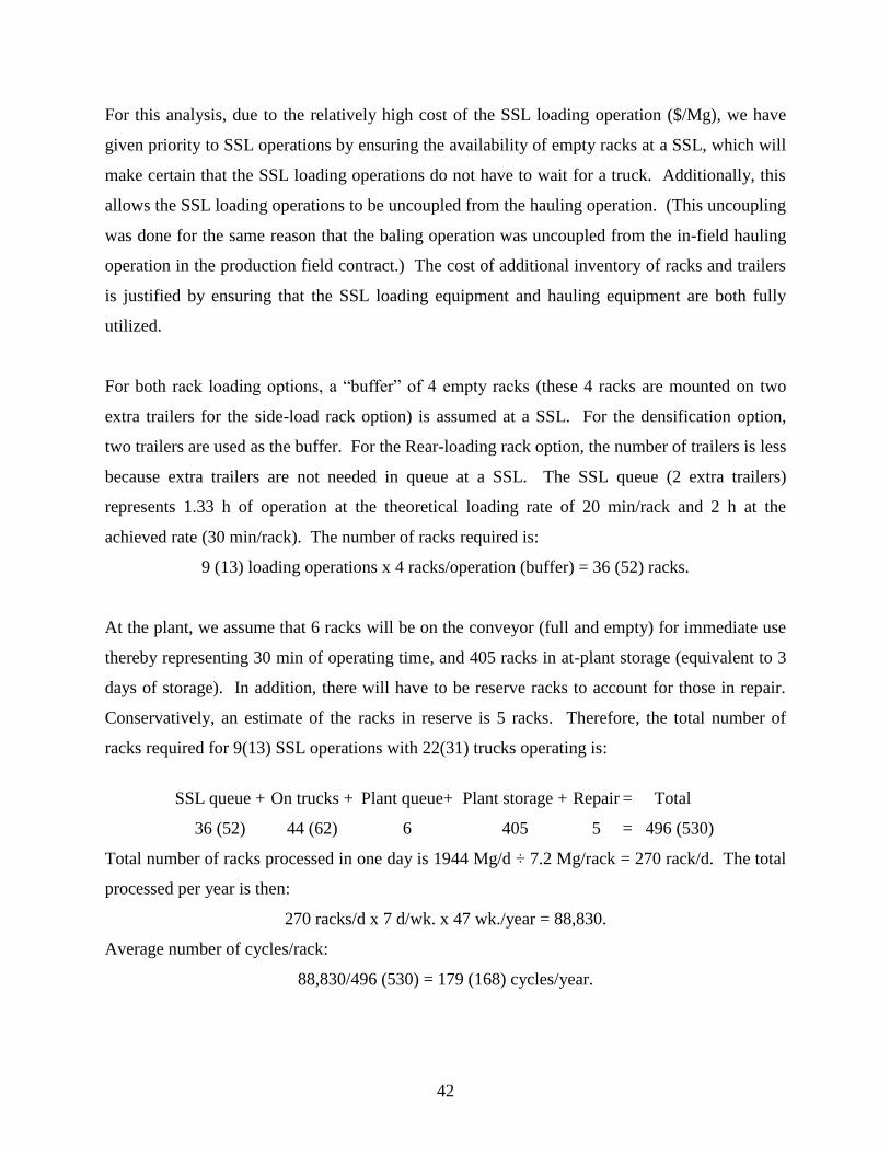
42

For this analysis, due to the relatively high cost of the SSL loading operation ($/Mg), we have

given priority to SSL operations by ensuring the availability of empty racks at a SSL, which will

make certain that the SSL loading operations do not have to wait for a truck. Additionally, this

allows the SSL loading operations to be uncoupled from the hauling operation. (This uncoupling

was done for the same reason that the baling operation was uncoupled from the in-field hauling

operation in the production field contract.) The cost of additional inventory of racks and trailers

is justified by ensuring that the SSL loading equipment and hauling equipment are both fully

utilized.

For both rack loading options, a “buffer” of 4 empty racks (these 4 racks are mounted on two

extra trailers for the side-load rack option) is assumed at a SSL. For the densification option,

two trailers are used as the buffer. For the Rear-loading rack option, the number of trailers is less

because extra trailers are not needed in queue at a SSL. The SSL queue (2 extra trailers)

represents 1.33 h of operation at the theoretical loading rate of 20 min/rack and 2 h at the

achieved rate (30 min/rack). The number of racks required is:

9 (13) loading operations x 4 racks/operation (buffer) = 36 (52) racks.

At the plant, we assume that 6 racks will be on the conveyor (full and empty) for immediate use

thereby representing 30 min of operating time, and 405 racks in at-plant storage (equivalent to 3

days of storage). In addition, there will have to be reserve racks to account for those in repair.

Conservatively, an estimate of the racks in reserve is 5 racks. Therefore, the total number of

racks required for 9(13) SSL operations with 22(31) trucks operating is:

SSL queue + On trucks + Plant queue+ Plant storage + Repair = Total

36 (52) 44 (62) 6 405 5 = 496 (530)

Total number of racks processed in one day is 1944 Mg/d ÷ 7.2 Mg/rack = 270 rack/d. The total

processed per year is then:

270 racks/d x 7 d/wk. x 47 wk./year = 88,830.

Average number of cycles/rack:

88,830/496 (530) = 179 (168) cycles/year.

43

If only the number of racks actively being used in the system (from the SSL queues, on the haul

trucks, and plant queue) are counted {86 (120)}, then each rack is filled and emptied 22 (16)

times each week. This would be the case if the racks were not used for at-plant storage, a

significant issue for future study.

Loaded racks at the SSLs at the end of the workday on Friday will, in commercial practice, be

towed in and emptied during weekend operations at the plant. These racks function as part of the

at-plant storage for weekend operations, thus the 405 racks listed for “Plant storage” is greater

than needed. These scheduling details must wait for a future study.

2.7.4 Total number of trailers required

The total number of trailers required for the hauling is estimated as follows. The total assumes an

extra 2 trailers for repair and maintenance for each of the three options. For the Rear-loading

rack system, no trailers are needed in the queue at a SSL. Note that an additional trailer is

required for each 2 racks in the SSL queue for the Side-loading rack option. The number of

bottom-dump trailers required for the Densification option is equivalent to the number of trailers

required for the Side-loading option. This results in 18 (26) additional trailers for the 36 (52)

racks in queue at a SSL.

SSL queue + With trucks + Repair = Total

Rear-loading option 0 22 (31) 2 = 24 (33)

Side-loading option 18 (26) 22 (31) 2 = 42 (59)

Densification option 18 (26) 14 (28) 2 = 34 (56)

2.8. Operations at the bio-crude plant and transportation to the

refinery

Any use of the biomass requires size reduction. This means that the round bales are chopped,

ground, or both. This section gives a brief overview of the operations involved in a grinding

operation at the BcP and some of the common conversion techniques that are currently being

studied.

44

2.8.1 Size reduction operations

As previously mentioned, we include a size-reduction operation at the plant for the two rack

options in order to achieve a fair comparison. We use the term “grinding” hereafter for the size-

reduction unit operation. Once a rack arrives at the receiving facility of the plant, the rack is

either queued for immediate use at the plant or placed in at-plant storage. The queue consists of

a conveyor to move the racks. The racks are then pulled from the queue and the individual bales

are removed by the use of a hydraulic ram to push bales from the rack so they fall individually

onto a conveyor for delivery to the grinding operation.

At a SSL, operations are only conducted for 10 h/d, 6 d/wk. However, at the plant, the biomass

is continuously ground during the 47 operating weeks. This allows the daily capacity of the

grinding equipment to be much higher due to the 24 h operations. The number of grinding

operations needed for the rack options is

.operations grinding 3.8 erMg/d/grind 510

Mg/d 1944

Hence, we assume that there are 4 sets of grinding operations operating continuously. In

practical terms, there will be four processing lines, each fed round bales for size reduction. Each

set of grinding operations requires 2 continuous employees, or 8 employees working three 8-h

shifts.

There are three components incorporated into the at-plant grinding operations costs: (1) the

grinder integrated into a system with suitable controls, (2) the prime mover (electric motor and

controls), and (3) dust control technology. The cost parameters for these three components are

presented in Table 2.2. No cost for the required utilities (electric power substation) or other

building cost parameters (structural features) is included in this example analysis.

2.8.2 Operations at the receiving facility

A BcP requires large volumes of biomass to ensure continuous operations. Therefore, the BcP

needs an industrial system for the rapid loading/unloading of trucks to maintain a constant flow

of material into the BcP and at-plant storage. Note that it would be difficult, or impossible, to

allow individual feedstock producers to deliver their respective biomass directly to the BcP.

45

Table 2.2: Equipment specifications for the grinding operations

Equipment

specifications for

grinding operations

Purchase

price ($)

Design life

(h)

R/M factor

($/h)

Energy

use

(kWh)a

Equip.

Cap. (Mg/h)

Equip. own.

cost ($/yr.)

Total Equip.

op. cost ($/h)

At-plant size reduction

Tub-grinder

377,500 15,000 1.43 - 22.7 202,249b

1.43

Electric motor 123,400 15 y 3%c

400.0

22.7 16,638d

26.91

Dust control tech. 200,000 5 y 6%c

20.0

22.7 53,691d 5.54

Total

268,723 33.88 a

b

c

d

We assume $0.08/kW h and a duty factor of 0.8

The equipment ownership cost is calculated using ASABE Standard ASAE EP496.3 FEB2006 Agricultural Machinery

Management and assuming: salvage value = 10%, interest rate = 8%, tax rate = 1%, and insurance = 0.8%.

The maintenance cost is a percentage of the purchase price, applied at an hourly cost assuming 7896 operating h/year

Calculated using a Capital Recovery Factor (CRF) plus tax rate = 1% and insurance = 0.8%

In the densification option of Morey et al., the grain trailers bottom-dump the flowable briquettes

at the plant and this material is immediately conveyed into a storage bin. The briquettes must be

placed in covered storage to ensure that there is no water penetration from precipitation.

Additionally, the storage will have to be actively managed (ventilated) to ensure it doesn’t

spontaneously combust. For this study, the same unloading time used for the racks, 10 min/load,

is used for the unloading of trailer loads of briquettes at the receiving facility.

In this study, we assume that all other operations at the plant (after size reduction) have an

identical cost. Regardless of the logistics option selected, management decisions must be made

to balance the cost of at-plant inventory and the risk of a plant shutdown due to insufficient

inventory.

2.8.3 Conversion techniques

Much of this review of conversion technologies follows an overview provided by McKendry

[97]. There are two major divisions within the conversion subject area, thermo-chemical

conversion and bio-chemical conversion.

Bio-chemical conversion techniques are divided into fermentation, anaerobic digestion, and

mechanical extraction. Mechanical extraction is used to extract oil from seeds like soybean and

cotton and does not apply for switchgrass.

46

Fermentation is used commercially to make ethanol from sugar crops, but switchgrass

conversion is more complex due to the longer-chain polysaccharide molecules that must be

broken down as a preliminary step (with an added cost). The biomass must be ground and dry.

The process is 40-90% efficient [78].

Anaerobic digestion is the conversion of organic material directly into a gas. This is done by

bacteria in an anaerobic environment. This is commercially available and requires a wet,

chopped material. The process is 10-40% efficient.

From these conversion technologies, we can see that the material must be at least chopped for all

cases, allowing for a size-reduced and flowable material to be produced at the entrance to the

conversion plant or earlier. Some allow for the material to be wet, in which case a liquid piping

system, not considered in this study, might be used.

Within thermo-chemical conversion techniques there are five major techniques: combustion,

gasification, pyrolysis, hydro-thermal upgrading, and liquefaction. The last two are only in their

research infancy.

With combustion, the biomass is simply burned to produce electricity or process steam, or both.

This is typically done at high temperatures ranging from 800-1000 . This biomass must be

somewhat dry and is often blown into the burner. For proper combustion it must be chopped to

less than 3 cm in size. The process is 20-40% efficient.

Gasification, much like direct combustion, requires high heat at a temperature between 800-

900 . The gas may be burned directly or be used as fuel for gas engines, gas turbines, and for

the production of methanol. This material must be prepared in the same way as is for

combustion, that is, it must be dry and at least chopped. This process is 40-50% efficient.

For pyrolysis conversion techniques, the biomass is converted into a liquid form by heating in

the absence of air to 500 . The liquid may be designated bio-crude or bio-oil depending on the

47

technique used. Again, the material must be dry and at least chopped. This process is up to 80%

efficient, but there are significant problems with stability of the bio-crude.

Hydro-thermal upgrading (HTU) and liquefaction are techniques that are still at pilot stage only.

HTU uses pressure to partly oxygenate hydrocarbons. Liquefaction has not proved successful

yet due to complex, expensive systems, but is done at a low temperature. In both cases, the

material is wet and needs to be at least chopped, and therefore, may be pumped into the plant as

a slurry.

2.8.4 Operations for transportation from the bio-crude plant to the refinery

There are two models that can be used to capture the relationship between the bio-crude plant

and the refinery. The first model, defined as the “large refinery model” recognizes the economy-

of-scale benefit achieved by increasing refinery size. The second model, defined as the “small

refinery model” envisions a structure that attempts to take advantage of the distributed nature of

a biomass resource and the smaller distribution area served by smaller refineries. Figure 2.5

depicts an aerial view of the two refinery models.

It has been well established by the petroleum industry that processing cost per unit of crude oil is

reduced with a high-capacity refinery. The refined products are then distributed to users over a

relatively large geographic area requiring a relatively high average distribution cost per unit of

refined product.

The small refinery model envisions small refineries located close to, or maybe adjacent to, bio-

crude plants. It may be that a refinery will just process the bio-crude from one plant, or,

depending on the size of the bio-crude plants, it will process oil from two or more bio-crude

plants. It is understood that the processing cost will be higher for a smaller refinery, and it will

increase as the refinery gets smaller. However, its benefit is that it would incur a lower cost to

distribute its products (over a smaller market area) because of its proximity to its customers.

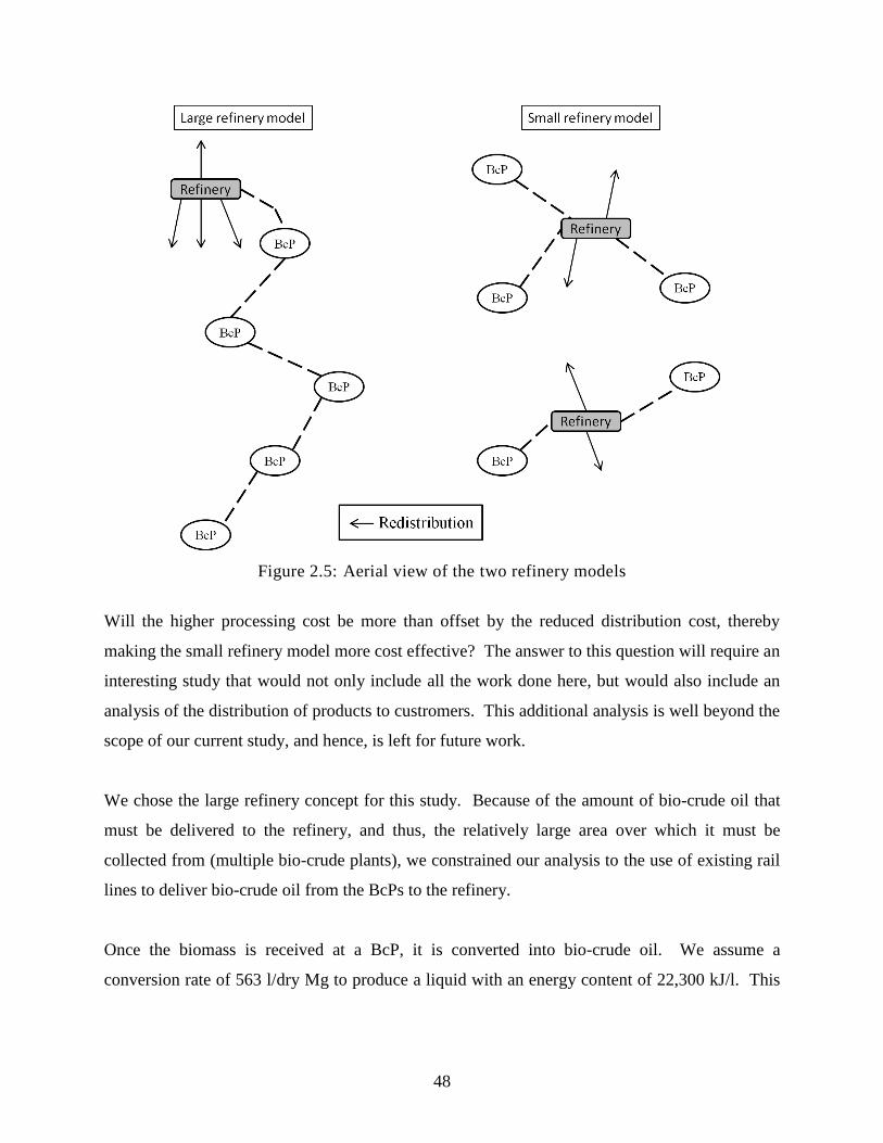
48

Figure 2.5: Aerial view of the two refinery models

Will the higher processing cost be more than offset by the reduced distribution cost, thereby

making the small refinery model more cost effective? The answer to this question will require an

interesting study that would not only include all the work done here, but would also include an

analysis of the distribution of products to custromers. This additional analysis is well beyond the

scope of our current study, and hence, is left for future work.

We chose the large refinery concept for this study. Because of the amount of bio-crude oil that

must be delivered to the refinery, and thus, the relatively large area over which it must be

collected from (multiple bio-crude plants), we constrained our analysis to the use of existing rail

lines to deliver bio-crude oil from the BcPs to the refinery.

Once the biomass is received at a BcP, it is converted into bio-crude oil. We assume a

conversion rate of 563 l/dry Mg to produce a liquid with an energy content of 22,300 kJ/l. This

49

bio-crude is a higher-value, more energy dense product than the raw biomass, which makes it

more practical to transport over large distances to a refinery.

It is envisioned that multiple BcPs would be located within the Piedmont to supply the large

amount of bio-crude needed for economy-of-scale operation at a refinery. A database was

created by replicating the real-life database for the 32-km radius around Gretna. These databases

were distributed along a rail line extending north and south from Gretna. The justification for

doing this is that the topography, soil types, and farming patterns are similar along this rail

corridor. This “corridor” database was then used for the optimization study presented in Chapter

4. The key constraints for this study are briefly described below.

The closest existing refinery to the production corridor used for our study is the Marathon

Petroleum Corporation refinery located at Catlettsburg, KY. (No statement of interest was

obtained from Marathon for our study.) We hypothesize that this refinery will expand operations

by adding a processing line to refine bio-crude in addition to its on-going production of

petroleum products.

The bio-crude is stored in temporary storage tanks in preparation for delivery to the refinery. A

detailed cost analysis of the rail car loading facilities at the bio-crude plant is provided in Table

2.3.

Table 2.3: Cost analysis for the rail car loading facilities at a bio-crude plant

Equipment systems Purchase

price ($)

Design life (y) R/M factor

($)

Energy use Own.

Costa ($/yr.)

Total op. costb ($)

Storage tanks 450,000 20 7,250/yr. 75/kW-hc 46,110 229,346/yr.

Yard Engine 430,000 20 12.00/h 15.14 l/hd 35,432 48.00/he

Individual Railcar Rental 9,600/y 9,773f a:

b:

c:

d: e:

f:

The equipment ownership cost is calculated using ASABE Standard ASAE EP496.3 FEB2006, assuming: salvage value = 10%, interest

rate = 8%, tax rate = 1%, and insurance = 0.8% Total Operating Cost = Repair and maintenance + Energy use + Labor (at $20/h)

Energy use in kW-h, we assume $0.08/kW-h and a duty factor of 0.8

We assume the cost of diesel fuel is $1.06/L ($4/gal.) The Yard engine’s equipment utilization is conservatively assumed to be 1 car/h

Including taxes (1%) and insurance (0.8%)

In general, the transportation of bio-crude oil from the BcPs can be achieved either via the road

network with tractor-trailer trucks or the rail network with tank cars. The first option, primarily

50

useful for short haul distances, allows the utilization of the road network and tractor-trailer trucks

for hauling the bio-crude from a BcP located off a rail line to a facility where it can be pumped

into rail cars for a longer transport distance. As alluded to earlier, we do not consider this option

for our study. We assume all BcPs are to be located along a rail line.) Truck hauling is well

known to have a relatively low setup/loading cost while having a higher cost per Mg-km to

transport when compared to rail transportation [82, 84].

Once at the refinery, the bio-crude is further processed through a deoxygenating process and is

thus upgraded to be equivalent to petroleum. Sixty-six percent of the bio-crude is refined into a

petroleum equivalent product, while the remaining mass in the bio-crude is a residue with other

applications [12, 14, 113]. Also, we assume that the conversion rate at a BcP is 563 l/Mg (135

gal/dry ton). If the 1944 Mg/d (1.35 Mg/min) of biomass being processed at the plant has

average moisture content of 15% wet basis, this amounts to 1652 dry Mg/h and the bio-crude

production is 930,000 l/d, which equals 5852 barrel bio-crude oil (bbo)/d. The products

produced by refining are then blended, stored, and shipped for final use. The focus of our study

is the chain of activities up to the point that bio-crude enters the refinery.

For the specific example presented here, we do not consider the cost to establish facilities at

either the BcP or the refinery. At a BcP, the bio-crude is expected to be stored in temporary

storage tanks for cyclic deliveries to the refinery. Additionally, we will assume that the refinery

is an average distance of 482 km (300 mi) from the BcPs. This is the actual distance from

Gretna, VA to the refinery in Catlettsburg, KY.

If the road network and the tractor-trailer trucks are used for direct delivery to the refinery,

operations can be semi-continuous for transporting the bio-crude. The following is a brief

analysis of an ideal hauling operation. Assuming an interstate transportation speed of 105 km/h

(65 mi/h) the haul time to travel 482 km would be 4.59 h not including loading/unloading times.

We assume the cycle time for a single truck to be 13 h including loading/unloading and rest time.

Assuming 19,650 l of haul volume, we need

trucks.30.2 l/load 19,650

h 13 x l/Mg 563 x h/d) (24

Mg/d 9441

51

Hence, if continuous operations were possible, 31 trucks would have to run without interruption

to haul the bio-crude from a single BcP to the refinery.

If instead of employing the road network and the trucks, the rail network is utilized, then the cost

of transporting the bio-crude can potentially be reduced significantly. Utilizing the rail-network

requires a larger storage system since the cycle time between runs is significantly greater. Cost

will be incurred for the purchase (or lease) of rail cars for permanent use. The railroad will own

the rail network and contract to transport the cars. If the average rail speed is 32 km/h (20 mi/h),

then the one-way haul time is 15 h.

In commercial operation, we expect the railroad will gather a unit train (entire train is all tank

cars filled with bio-crude) and make one weekly delivery to the refinery. With coal, grain, and

other unit train operations, a unit trial is typically 100+ cars.

We assume one day to fill and one day to unload the needed cars. This results in a cycle time of

3 days. We assume that a BcP is emptied weekly and that each rail car has a haul volume of

90,850 l (24,000 gal.). Then the number of cars needed per week to haul from our example BcP

to the refinery is

cars. rail 84.3 car l/rail 90,850

l/Mg 563 x d 7 x Mg/d 1944

This would require the necessary storage at a BcP to be able to hold a week’s worth of inventory

of bio-crude, resulting in a storage capacity of approximately 7660 m3 (7,660,000 l). Several

tanks, in effect, a “bio-crude tank farm”, will be required.

2.9. Application to a real-life scenario

The above description of BcP plant operations was applied to a real-life potential production

region in South-central Virginia. The database developed for this scenario was described by

Resop et al. [118]. Three datasets were generated where the largest two datasets are the same as

the dataset generated by Resop et al. The three datasets correspond to potential production fields

within 13-, 32-, and 48-km radii from a potential BcP in Gretna, VA, where the total production

land was estimated to be 6% of the total area within the given radius. The purpose of the

52

smaller, 13-km dataset is for comparing the three model formulations in Chapter 3 since one

formulation, without decomposition, is too large to get a solution.

2.9.1 GIS database management

The 32- and 48-km databases initially contained at total of 13,344 and 29,782 production fields,

respectively. Through data reduction techniques described in this section, the production fields

were merged to reduce the level of detail in the model. These were then randomly selected until

a land utilization rate of 6% was obtained. The 13-, 32-, and 48-km radii datasets have a total of

3099, 19,304, and 43,434 ha with 299, 1584, and 3655 production fields and 47, 261, and 589

potential SSLs, respectively. The total yield from these production fields is large enough to

provide 6, 37, and 83 Mg/h of biomass for a BcP operating continuously for 47 week/year, which

compares to the 81 Mg/h plant size used in the example calculations given earlier in this chapter.

In the database provided by Resop et al. [118], data was collected to locate the land that could

potentially be attracted into the production of switchgrass. In order to reduce the amount of

memory required to store relevant information, the following aggregation approach was utilized:

1. If the center points of a set of production fields were within 200 m of each other, then the

production fields were merged into one larger production field with a new center-point

calculated using the weighted average of each production field.

2. If a merged production field resulting from step 1 had more than 10 production fields, then a

150-m distance was used instead to reduce the area of a cumulative production field.

3. If a merged production field resulting from step 2 had more than 10 production fields, then a

130-m distance was used instead to reduce the area of a cumulative production field.

4. If the resulting total area of an aggregated production field was less than 15 ha, then this

production field was merged with the nearest production field with more than 15 ha.

Steps 1-3 reduce the data by aggregating the production fields that are near to one another into a

larger production fields. Step 4 reduces the size of the data by merging production fields that

would not have a significant contribution to the model due to a relatively small amount of

biomass harvested from them. This helps in capturing reality since owners of small parcels of

53

land are expected to contract with larger producers to have their biomass harvested and hauled to

a SSL rather than harvesting and hauling the biomass themselves.

To prepare the aggregated data for analysis, the production fields from the Resop study were

imported into ArcGIS version 9.3.1, and then, overlaid with a road network, slope,

urban/residential, and streams/lakes data. From the slope layer, locations with a slope less than

10% grade were selected while buffers were created for the urban/residential and streams/lakes

layers. Four requirements are provided for a production field to be considered as a SSL: (1) it

must be on a state-maintained, primary/secondary road, (2) it should not be within 100 m of

primary water bodies, (3) it should not be within 500 m of urban locations, and (4) its average

slope must be less than 10%. Priority is given to scrubland or grassland with at least 40 ha of

potential production fields available within a 3.2-km radius. All the production fields that met

the criteria were selected as potential SSLs. These potential SSLs represent the z-variables in the

formulations proposed in Chapter 3. The distances and respective costs associated with the c-

and d-variables (defined in Chapter 3) were calculated using the actual road network distances in

ArcGIS. Once the data was collected, it was then exported to a database file to interface with

CPLEX 12.1.0.

An additional dataset was created that consisted of only the potential SSLs that Resop et al.

selected to generate the solution to their problem. In the Resop study, SSLs were manually

selected in order to maintain a uniform distribution of SSLs over the entire region. This resulted

in 99 and 199 SSLs for the 32- and 48-km datasets, respectively, each storing biomass from

production fields within a radius of 3.2 km (2 mi). This additional database was used to compare

the cost of using Resop’s manually-selected SSLs (designated as Resop-Fixed) with the cost of

99 and 199 optimally selected SSLs (designated as Optimal-Fixed).

2.9.2 Parameter setting

It is assumed that the annual yield rate of switchgrass is deterministic with a yield of 15 Mg/ha

[44, 139]. Cundiff et al. [23] estimate the cost to transport switchgrass as a 1.5-m diameter

round bale from production field i to SSL j to be where the unit of is

defined in terms of $/km/Mg. The costs incurred for hauling biomass from SSL j to the BcP by

54

the two Rack Systems and the Densification System, with their respective capacities of 14.4 and

22.7 Mg/haul, are estimated to be and respectively,

assuming 10 min load and unload times, $800/day truck operating cost, 10 h/day hauling, and an

average haul speed of 72 km/h (45 mi/h). These costs are similar to those presented in Searcy et

al. [125] after accounting for the faster load/unload times; see also [74, 82, 84]. These costs are

accounted for as a part of the parameter defined in Chapter 3.

The equipment ownership cost represents the cost of equipment, taxes, and insurance. The

equipment operating cost represents the cost of repair (R), maintenance (M), labor, and diesel

fuel use. The equipment ownership and operating costs for each system are presented in Table

2.4 where the equipment’s capacity is scaled to 70% of theoretical capacity to account for

operational delays. (The equipment ownership cost is calculated using ASABE Standard ASAE

EP496.3 FEB2006 Agricultural Machinery Management and assuming: salvage value = 10%,

interest rate = 8%, tax rate = 1%, and insurance = 0.8%.) The cost for operating the equipment

per Mg (including labor cost) is factored into the parameter (defined in Chapter 3) for all of

the models. Grinding operations at the BcP for the rack systems are assumed to run continuously

when the plant is operating, resulting in a much higher annual use capacity (7896 h/year).

For the grinding operations, it is emphasized that the dust control subsystem cost may be under-

estimated. To ensure a fair comparison with the Densification System, the cost of owning and

operating the necessary at-plant size reduction equipment (including labor cost) is calculated

directly and added to the objective function value for the two rack systems.

For this study, we simplify the above rack analysis and assume that the number of racks needed

per equipment set is 8. This allows for 4 racks to be in queue at a SSL (for loading) while 2

trucks are transporting the other 4 racks. More trucks and racks would be required if the average

travel distance is greater than 36 km.

The queue of racks and/or trailers at a SSL ensures that the equipment at the SSL is fully utilized

and does not have to wait for a truck to arrive to continue loading. As previously mentioned, the

total number of required trucks and trailers may be further reduced by optimally scheduling the

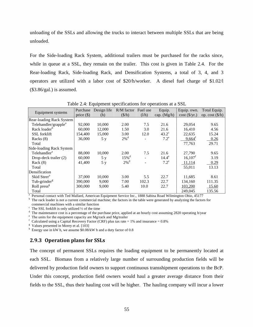
55

unloading of the SSLs and allowing the trucks to interact between multiple SSLs that are being

unloaded.

For the Side-loading Rack System, additional trailers must be purchased for the racks since,

while in queue at a SSL, they remain on the trailer. This cost is given in Table 2.4. For the

Rear-loading Rack, Side-loading Rack, and Densification Systems, a total of 3, 4, and 3

operators are utilized with a labor cost of $20/h/worker. A diesel fuel charge of $1.02/l

($3.86/gal.) is assumed.

Table 2.4: Equipment specifications for operations at a SSL

Equipment systems Purchase

price ($)

Design life

(h)

R/M factor

($/h)

Fuel use

(l/h)

Equip.

cap. (Mg/h)

Equip. own.

cost ($/yr.)

Total Equip.

op. cost ($/h)

Rear-loading Rack System

Telehandler/grapplea 92,000 10,000 2.00 7.5 21.6 29,054 9.65

Rack loaderb 60,000 12,000 1.50 3.0 21.6 16,410 4.56

SSL forklift 154,400 15,000 3.00 12.0 43.2c 22,635 15.24

Racks (8)

36,000 5 y 2%d - 7.2

e 9,664

f 0.26

Total 77,763 29.71

Side-loading Rack System

Telehandlera 88,000 10,000 2.00 7.5 21.6 27,790 9.65

Drop-deck trailer (2) 60,000 5 y 15%d - 14.4

e 16,107

f 3.19

Rack (8) 41,400 5 y 2%d - 7.2

e 11,114 0.29

Total

55,011 13.13

Densification

Skid Steera 37,000 10,000 3.00 5.5 22.7 11,685 8.61

Tub-grinderg 390,000 9,000 7.00 102.3 22.7 134,160 111.35

Roll pressg 300,000 9,000 5.40 10.0 22.7 103,200 15.60

Total 249,045 135.56 a

b

c

d

e

f

g

h

Personal contact with Ted Mallard, American Equipment Service Inc., 1888 Sabina Road Wilmington Ohio, 45177

The rack loader is not a current commercial machine; the factors in the table were generated by analyzing the factors for

commercial machines with a similar function

The SSL forklift is only utilized ½ of the time

The maintenance cost is a percentage of the purchase price, applied at an hourly cost assuming 2820 operating h/year

The units for the equipment capacity are Mg/rack and Mg/trailer

Calculated using a Capital Recovery Factor (CRF) plus tax rate = 1% and insurance = 0.8%

Values presented in Morey et al. [103]

Energy use in kW h, we assume $0.08/kW h and a duty factor of 0.8

2.9.3 Operation plans for SSLs

The concept of permanent SSLs requires the loading equipment to be permanently located at

each SSL. Biomass from a relatively large number of surrounding production fields will be

delivered by production field owners to support continuous transshipment operations to the BcP.

Under this concept, production field owners would haul a greater average distance from their

fields to the SSL, thus their hauling cost will be higher. The hauling company will incur a lower

56

cost because they do not have to move loading equipment from one SSL to the next. The

concept is represented by the “BLP” designation in Chapter 3.

Instead of keeping the loading equipment permanently at each SSL, another method to operate

SSLs is to move this equipment from one SSL to the next. This would allow the number of SSLs

to be greater in number and more widely distributed. The average haul distance from a

production field to a SSL will be reduced, and thus, the average haul cost to a production field

owner will be reduced as well. The hauling contractor, however, must now bear the cost of

moving their equipment from one SSL to the next. This concept is represented by the “BLP-M”

designation in Chapter 3. For modeling purposes, the BLP-M model is then decomposed and

solved in two stages. In the first stage, the SSLs are located and the production fields are

allocated to SSLs. In the second stage of the model, the cost of moving the equipment from one

SSL to the next is minimized.

The minimum SSL size is 3 days of loading operations , and the maximum SSL

size is 30 days of loading operations . The value for E, the maximum annual

handling capacity of an equipment set unloading SSLs, is 2985 ha, which is 70% of the

theoretical value of 4265 ha. The total amount of biomass to be processed at the plant in terms

of hectares, is 80% of the total available biomass in order to allow the model to select the best

production field locations.

Table 2.5 presents results based on the information from Table 2.4 combined with the analysis

described in Chapter 3. The “Avg. equip. cost” is the total equipment cost divided by the total

annual biomass handled by the equipment. The “Avg. operating cost/Mg” is given by

{total equip. operating cost ($/h) + No. Workers x ($20/h)} / equip. capacity (Mg/h).

These costs include the cost of the grinding operations at the plant but exclude the cost of the

racks in inventory at the plant to ensure a fair comparison of cost.

57

Table 2.5: Overview of results for transportation from the SSLs to the bio-crude plant

No. of

SSL

operations

No. of

workers

No. of

Racks

No. of

Trailers

No. of

plant

Grinders

No. of

Trucks

Mg/haul Avg.

equip.

cost/Mg

Avg.

operating

cost/Mg

Rear-loading 9 (13) 4 496 (530) 24 (33) 4 22 (31) 14.4 5.99 (7.89) 18.20 (20.11)

Side-loading 9 (13) 3 496 (530) 42 (59) 4 22 (31) 14.4 2.48 (2.82) 7.43 (7.78)

Densification 9 (13) 2 0 34 (56) 0 14 (28) 22.7 3.50 (5.06) 11.24 (12.80)

Note: The “()” represent the expected results

The Rear-loading, Side-loading and Densification options have an average operating cost per Mg

of $18.20, $7.43, and $11.24, respectively, for delivery of biomass from within a 48-km radius

around Gretna, VA (when assuming uniform distribution). Our analysis showed that the Side-

loading rack option is preferred for transporting the biomass over distances less than 81.5 km.

For distances greater than 81.5 km, the Densification option is preferred due to a reduction in

cost that results from achieving a maximum mass per truckload.

2.9.4 Parameter setting-for transportation from the bio-crude plant to the

refinery

The cost for transporting bio-oil via truck and rail are both well-defined in the literature. Table

2.6 presents a review of cost parameters for the road transportation of bio-mass in various forms.

The differentiation in costs is a result of differences in equipment usage. The cost presented by

Henrich et al. [67] is for the transportation of biosyncrude, a product essentially the same as the

bio-crude oil in our study. Table 2.7 presents the cost for utilizing a rail-network in the United

States. We define “Fixed shipper cost” as the setup cost for loading the biomass at the rail

station and “Transportation cost” as the cost to move the biomass from one location to another.

2.9.5 A simplified analysis

If we assume the average travel distance from the production field to a SSL to be 3 km, then this

results in a cost of $5.11/Mg. We add this cost to the average operating cost presented above for

the three equipment options, and then, consider the cost to transport the biomass to the BcP using

the cost parameters presented above. The results are presented in Table 2.8, where the unit for

the fixed cost is $/Mg and for the transportation cost is $/Mg/km.

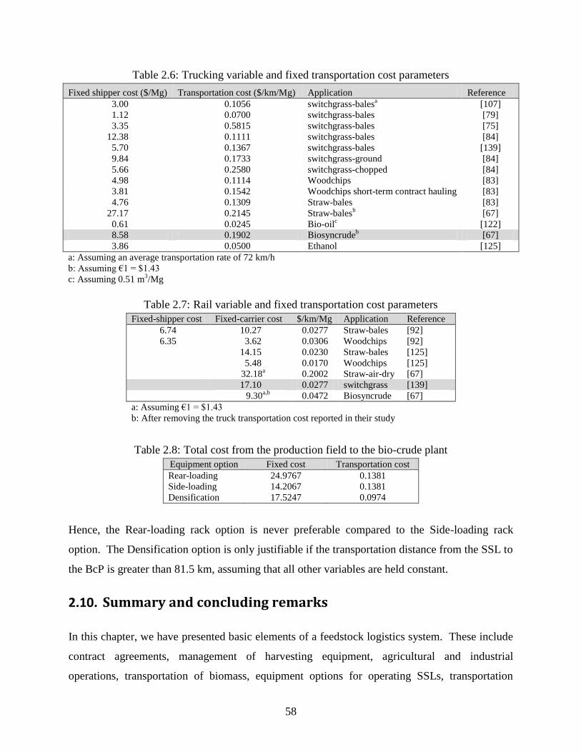
58

Table 2.6: Trucking variable and fixed transportation cost parameters

Fixed shipper cost ($/Mg) Transportation cost ($/km/Mg) Application Reference

3.00 0.1056 switchgrass-balesa [107]

1.12 0.0700 switchgrass-bales [79]

3.35 0.5815 switchgrass-bales [75]

12.38 0.1111 switchgrass-bales [84]

5.70 0.1367 switchgrass-bales [139]

9.84 0.1733 switchgrass-ground [84]

5.66 0.2580 switchgrass-chopped [84]

4.98 0.1114 Woodchips [83]

3.81 0.1542 Woodchips short-term contract hauling [83]

4.76 0.1309 Straw-bales [83]

27.17 0.2145 Straw-balesb

[67]

0.61 0.0245 Bio-oilc [122]

8.58 0.1902 Biosyncrudeb

[67]

3.86 0.0500 Ethanol [125]

a: Assuming an average transportation rate of 72 km/h

b: Assuming €1 = $1.43

c: Assuming 0.51 m3/Mg

Table 2.7: Rail variable and fixed transportation cost parameters

Fixed-shipper cost Fixed-carrier cost $/km/Mg Application Reference

6.74 10.27 0.0277 Straw-bales [92]

6.35 3.62 0.0306 Woodchips [92]

14.15 0.0230 Straw-bales [125]

5.48 0.0170 Woodchips [125]

32.18

a 0.2002 Straw-air-dry

[67]

17.10 0.0277 switchgrass [139]

9.30

a,b 0.0472 Biosyncrude [67]

a: Assuming €1 = $1.43

b: After removing the truck transportation cost reported in their study

Table 2.8: Total cost from the production field to the bio-crude plant

Equipment option Fixed cost Transportation cost

Rear-loading 24.9767 0.1381

Side-loading 14.2067 0.1381

Densification 17.5247 0.0974

Hence, the Rear-loading rack option is never preferable compared to the Side-loading rack

option. The Densification option is only justifiable if the transportation distance from the SSL to

the BcP is greater than 81.5 km, assuming that all other variables are held constant.

2.10. Summary and concluding remarks

In this chapter, we have presented basic elements of a feedstock logistics system. These include

contract agreements, management of harvesting equipment, agricultural and industrial

operations, transportation of biomass, equipment options for operating SSLs, transportation

59

equipment needs, and operations at a bio-crude plant. We have also highlighted the impact that

the decisions at the production field level have on the cost and implementation of the logistics

system. To this end, it is essential that the decisions concerning the production field operations

must be made in view of their impact on the entire system.

The key decisions made for use in our analysis of a biomass logistics system are as follows:

The region chosen for study is the Piedmont of the Southeastern United States, a

physiographic region with much under-utilized cropland. This land can be used for

production of bio-energy with minimal competition with food production.

Switchgrass, a native warm-season grass, was chosen as the model herbaceous species. It

can be harvested over a 9-month season in the Piedmont.

The round bale is chosen because its rounded top allows it to protect itself from rain

penetration. This allows the uncoupling of the baling and in-field hauling operations. It

also allows for single-layer ambient storage in a SSL, which avoids the higher cost of

covered storage.

The business plan envisions that a production field owner will deliver biomass to a SSL

and will be paid at that point. A hauling contractor, hired by the BcP owner, loads and

hauls biomass to the BcP in order to meet the required weekly demand schedule. No

analysis of the delivery of biomass to the SSLs and of operations at the receiving facility

of the BcP was undertaken.

A multi-bale handling unit, a 16-bale rack, is used to deliver raw biomass. The

performance of this option is compared with that of processing raw biomass into

briquettes and the use of mobile equipment at the SSLs. The higher bulk density for the

load of briquettes allows the truck to be loaded to road-legal weight.

A BcP receives raw biomass from production fields within a predefined radius. Real-life

databases for a 32-km and 48-km radius around Gretna, VA will be used.

The BcP converts the raw biomass into a liquid intermediate, called bio-crude oil. Bio-

crude oil has a much higher energy density than that of the raw biomass, and it has the

advantages of being handled as a liquid.

60

The analysis presumes a large refinery to obtain an economy-of-scale benefit in the

refining of bio-crude into products for existing commercial markets. Multiple BcPs load

tank cars for rail shipment to a refinery. It is envisioned that the railroad will gather a unit

train (100 cars) each week and deliver to the refinery.

61

Chapter 3 Design, Modeling, and Analysis of a Feedstock Logistics System to Serve a Bio-crude Plant

3. Hidden figure

Table 3: Hidden table

3.1. Description of the biomass logistics system

The feedstock logistics system designed for transporting biomass from production fields to the

BcP has application in almost all types of feedstock used in the bio-crude industry. The key

items that need to be determined are the locations of satellite storage facilities (SSLs), the order

in which to unload the SSLs, the number of equipment sets to use, the location of the BcP, and

inventory levels at both the SSLs and the BcP. In this chapter, it is assumed that a location of

the BcP is known a priori, and also, enough space is available at the plant to accommodate the

biomass supplied by the SSLs.

The transportation problems associated with the feedstock logistics system are similar in nature

regardless of the conversion technique used at the BcP. This is because the raw biomass has a

relatively low haul-density (Mg/m3), which requires multiple hauls across a large coverage area

in order to satisfy the demand at an industrial-size BcP, where haul volume is a limiting factor

instead of load capacity. In this chapter, the problem is addressed for designing a feedstock

logistics system that minimizes the cost of transporting biomass from the production fields to the

BcP. It is assumed that the biomass is accumulated at satellite storage locations (SSLs) by

feedstock producers who are within 13-, 32-, and 48-km radii of a pre-located BcP. Each SSL is

an uncovered gravel lot that is relatively close to the main highways or paved (secondary) roads,

and it is the storage point for either a single large production field or multiple smaller fields as

proposed by Cundiff et al. [22]. The SSLs in our case play the same role as the use of

“warehouses” by Zhu et al. [154] and “local storage” by Morey et al. [103]. In this chapter, the

focus is on the delivery of 1.5-m diameter, 0.45 Mg dry round bales that are commonly used in

the Southeastern United States because of their ability to shed water in single-layer ambient

storage, thus avoiding the relatively high cost of covered storage.

62

3.1.1 Transportation of biomass from production fields to satellite storage

locations

A production field is assumed to be independently operated by a feedstock producer. No limit is

placed on the minimum size of a production field. This is motivated by the desire to encourage

participation of producers of all sizes in the production of biomass, and thereby achieving

maximum benefit to the local economy. The cost associated with growing, maintaining, and

harvesting the biomass is included in a contract price paid to the producer, and therefore, these

costs are not considered in this study. However, the cost of transporting the biomass from the

production fields to the SSLs is incorporated, although this function is performed by feedstock

producers with their own equipment. It is assumed that a “production field-gate” contract is in

place to pay the feedstock producer to grow, harvest, transport and store round bales at the SSLs.

A storage cost to establish and maintain a SSL is included in each production field-gate contract.

One of several critical issues in the delivery of feedstock is the high cost of transporting round

bales using the producer’s in-field hauling equipment, operated both in field conditions and on

paved roads. Such equipment has a limited road speed, thereby making it less efficient than a

tractor-trailer truck. Hence, the concept of satellite storage locations (SSLs) is used to provide

for the “least possible travel distance” between a production field and the selling point (a SSL).

From a system cost perspective, the SSLs must be located in order to strike a balance between

the cost of developing the SSLs, transporting biomass from the production fields to the SSLs,

and loading of biomass at a SSL for transporting it to the BcP. In this study, it is assumed that

the biomass is always available at the SSLs, thereby requiring the feedstock producers to

transport the biomass and to maintain necessary inventory at each SSL in accordance with the

needs of the BcP.

3.1.2 Operations at a satellite storage location

Three equipment systems are considered for the operations performed at a SSL. Each of these

systems is similar with regard to the implementation of rapid load/unload times for the

transportation of biomass from a SSL to the BcP. However, the key differences are in the cost of

owning and operating the equipment required.

63

Two systems utilize the rack concept first described by Cundiff et al. [22]. Ravula et al. [116,

117] propose a round bale logistics system utilizing this rack system. A rack system does not

perform any additional densification, and consequently, results in a higher truck transportation

cost because of volume limitations. The racks have dimensions that emulate a 6.1-m (20-ft) ISO

container providing two levels of 8 bales to be handled as a single 16-bale unit. A tractor-trailer

truck, using a drop-deck trailer to meet the height regulations within the United States, can haul

two racks (32 bales, 14.4 Mg) per load.

At a SSL utilizing the rack system, the round bales of biomass are handled in one of two ways.

The first rack system loads bales into the rack from the rear and is referred to as the “Rear-

loading Rack System.” For this system, the cycle of operations at a SSL is as follows: (1) empty

racks are unloaded from the drop-deck trailers onto a specialized bale-loading machine using an

industrial-size forklift, (2) bales are then put into the bale-loading machine via a telehandler

(lifting four bales at-a-time), and (3) once the rack has been filled, it is staged and subsequently

loaded onto a tractor-trailer truck upon its arrival.

The second rack system, referred to as the “Side-loading Rack System,” loads bales of biomass

into a rack from the side, thereby requiring an open side rack design. A telehandler loads the

bales two at-a-time while the rack remains on the trailer, thus avoiding (1) the requirement for

the industrial-size forklift to handle loaded racks and (2) use of the specialized bale-loading

machine. Tractor-trailer trucks drop a trailer with two empty racks at a SSL and pick up a trailer

with two loaded racks. This system requires a single telehandler at a SSL and additional drop-

deck trailers sitting in queue at a SSL to be loaded.

A third system densifies bales of biomass into a briquette at the SSLs. Densification increases

the energy density of a load, and it has been shown to be a useful operation early in the logistics

supply chain. Two independent studies, in Japan [152] and in Finland [114, 115], have reported

that the tradeoff between the cost of densification and reduction in transportation cost for logging

residues are significant, thereby making densification a viable option for transport of raw

biomass.

64

Morey et al. [103] presented a densification system for round bales of corn stover. In this

chapter, the Morey et al. system is designated as the “Densification System.” In this system, a

skid steer loader loads bales into a tub-grinder. The ground material is then delivered to a roll

mill via a conveyor where it is pressed into briquettes. These briquettes are loaded into a grain

trailer (open top, hopper bottom) for transporting and unloading. To minimize truck waiting

time and to ensure constant utilization of equipment, an empty trailer is exchanged with a loaded

trailer when the truck arrives at a SSL. The Densification System increases the bulk density of

the biomass to at least 240 kg/m3, thereby allowing for a full load capacity (27.7 Mg). For

additional work in densification subject area, see [4, 24].

Due to the fact that the final product must be ground ahead of to any conversion process at the

plant, the grinding operation is a value-added process. For this reason, the cost of grinding the

biomass at the plant is included for both rack options so that all three options can be compared at

the same end point. The at-plant grinding operation has three subsystems. The first subsystem

consists of a tub-grinder, knuckle-boom loader, and a belt conveyor. The second subsystem

consists of a 400-kW electric motor with controls. The third subsystem is a dust control system.

For all three SSL equipment systems, the SSL equipment may be either placed permanently at

the SSL or it may be designed to be mobile and moved from one SSL to another as each SSL is

unloaded. Due to the high cost of locating stationary equipment at a SSL, a larger coverage area

is required to fully utilize the equipment, thereby requiring the producers to haul the round bales

from a farther distance to the SSL. On the other hand, the mobile equipment system allows the

SSLs to be relatively small, which reduces the producer’s costs for hauling the biomass.

3.1.3 Operations at the receiving facility

The BcP requires large volumes of biomass to ensure a continuous operation, and therefore, it

needs an industrial system for the rapid loading/unloading of trucks to maintain a constant flow

of material into the BcP directly or into at-plant storage. This makes it difficult, or impossible, to

allow individual feedstock producers to deliver their respective biomass directly to the BcP. For

the 13-, 32-, and 48-km datasets utilizing approximately 6% of the total land, the plant would

65

require 0.93, 5.70, and 12.84 loads/h, respectively, assuming that the delivery operations take

place 10 h/day, 6 day/week, and 47 week/year (2820 h/year).

For both rack systems, the racks are removed at the BcP, and the empty racks are then placed on

the tractor-trailers to be returned to a SSL. The racks at the plant are either queued for

immediate use or placed in at-plant storage for later use. In the Densification System, the grain

trailers bottom-dump the briquettes at the plant. The briquettes must be placed in a covered

warehouse to ensure that there is no water penetration from precipitation. For this study, the

unloading of racks at the receiving facility is assumed to require a total of ten minutes. Once the

biomass is at the BcP, it must be chopped and/or ground before use.

3.2. Problem statement and mathematical formulations of the

feedstock logistics problem

The problem addressed in this chapter can be concisely defined as follows: Given f production

fields and n potential locations for SSLs, determine the optimal number of SSLs and their

respective locations (on a subset of production fields), and the allocation of production fields to

SSLs so as to minimize the total cost incurred: (1) from transporting biomass from each

production field to a SSL, (2) for the purchasing and use of equipment to empty the SSLs, (3) for

the subsequent transportation of the biomass (densified or undensified depending upon the

option used) from SSLs to the BcP, (4) during routing of loading equipment among the SSLs, and

(5) for use of labor. This problem is designated as the Biomass Logistics Problem (BLP-F) if the

loading equipment is placed permanently at each SSL and BLP-Mobile (BLP-M) if the loading

equipment is allowed to move from one SSL to another. A mixed-integer, linear programming

(MILP) formulation is used to model both of these problem instances. The routing of equipment

among the SSLs results in a multiple asymmetric traveling salesmen problem (mATSP), which is

an additional feature of BLP-M.

The selection of a production field on which to build a SSL and the allocation of biomass from

other production fields to that SSL is similar to a location-allocation problem. A review of work

for this problem can be found in Melo et al. [98] and Owen and Daskin [109].

66

The work reported in the biomass logistics area can be divided into two categories: stochastic or

deterministic, and integer or continuous. In the stochastic area, Kumar and Sokhansanj [84] have

presented an integrated biomass supply analysis and logistics model (IBSAL), which captures

the stochastic biomass logistics issues such as variability in processing as a result of weather,

time, equipment breakdowns, etc. Additional work in this area can be found in De Mol et al.

[28], Nilsson [106], and Ravula et al. [117]. In the deterministic area, most of the reported work

utilizes a geographic information system (GIS) interactively with an optimal seeking heuristic

solver. Most of the deterministic models presented are mixed-integer programs [50, 75, 93, 141,

142]. Continuous models assume that all the land within a region is utilized for biomass

production [103, 104]. This approach uses average haul distances and cost, and therefore, the

solution obtained is difficult to implement due to lack of detail, as opposed to the solution

obtained using an integer model formulation, where each production field is considered as a

specific entity with specific costs, thereby resulting in precise decisions for implementation.

The models presented herein are discrete and deterministic formulations that also utilize GIS for

data management. However, they are different from those presented in the literature due to the

consideration of the SSLs for local storage of biomass and the use of mobile loading equipment

to move from one SSL to another.

In a recent paper published by Zhu et al. [154], a detailed model is presented that is similar in

many aspects to the work presented herein. Their work effectively models the operations

required in the logistics system for a BcP. However, the formulation is effective only for

aggregated data, which overlooks the details required for real-life implementation. The BLP

formulation presented in this chapter seeks a balance between model detail and data detail in

order to provide meaningful information to end users for practical implementation.

The BLP-F model formulation determines the locations for the SSLs and allocates production

fields to each of the SSLs selected. Consider the following notation:

67

Permanent equipment parameters:

l

ijd

cost to transport biomass from production field i to SSL j with equipment system l,

including the cost to grind and/or densify the biomass for equipment systems 1 and 2,

and transportation to the BcP, 3 ,2 ,1 ,,...,1 ,,...,1 lnjfi

P

js

rental, developmental, and equipment purchasing cost for utilizing permanent

equipment at SSL j (paid to the production operator on which SSL j is placed),

nj ,...,1

iha

size of production field i (ha),

fi ,...,1

E

maximum processing capacity of each equipment set (ha)

BeP

maximum processing capacity of each equipment set (ha)

Decision variables:

ijy

1, if production field i transports biomass to the BcP through SSL j

0, otherwise, njfi ,...,1,,...,1

jz

1, if potential SSL j is selected as a SSL

0, otherwise, nj ,...,1

The following formulation is developed for the BLP-F problem, where the loading equipment (l)

is permanently placed at each SSL.

BLP-F: Minimize

f

i

n

j

ij

l

ij yd1 1

n

j

j

P

j zs1

(3.1)

subject to:

,yn

j

ij 11

fi ,...,1 (3.2)

,jij zy njfi ,...,1,,...,1 (3.3)

, 1

j

f

i

iji zEyha

n,...,j 1 (3.4)

BePyhaf

i

n

j

iji 1 1

(3.5)

},1,0{jz ;,...,1 nj },1,0{ijy

.,...,1,,...,1 njfi (3.6)

68

The objective function consists of the total cost of transporting biomass from the production

fields to the BcP plus the cost incurred at the SSLs. Constraints (3.2) capture the fact that every

production field is allocated to at most one SSL. Constraints (3.3) assert a SSL to be utilized

only if it is opened. Constraints (3.4) ensure that each equipment set does not exceed its annual

capacity, while Constraint (3.5) ensures that enough biomass is collected to satisfy the minimum

processing capacity of the BcP. Note that Constraint (3.5) will always be tight because the

objective function represents cost and not revenue. If revenue from the sale of bio-crude (via

power, biofuel, etc.) were captured, then Constraint (3.5) could potentially be exceeded.

However, due to high variability in the currently-used conversion process and sales of biofuels,

these revenues are not included in this study. Constraints (3.6) constitute logical requirements on

the decision variables.

Next, the parameters, variables, and a formulation are presented for the case when the loading

equipment is allowed to travel from one SSL to another. This formulation is designated as BLP-

M.

Mobile equipment parameters:

M

jkc

cost to move mobile equipment from SSL j to SSL k, kjnkj ,,...,1,

M

kc0 purchasing cost of an equipment set. Note that “0” is assigned as a dummy (base)

SSL from where the tour of an equipment set begins, if it is utilized. For its first leg,

an equipment set can visit any SSL. Therefore, it is defined .,...,1 nk Thus, the

cost incurred for the first leg of an equipment’s tour represents its purchase cost

M

js

rental/development fee for utilizing SSL j, including a fixed cost for the

setup/takedown of equipment nj ,...,1

minS

minimum allowable size of a SSL (3 days of loading)

maxS

maximum allowable size of a SSL (30 days of loading)

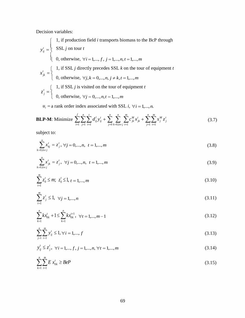
69

Decision variables:

t

ijy

1, if production field i transports biomass to the BcP through

SSL j on tour t

0, otherwise, mtnjfi ,...,1 ,,...,1 ,,...,1

t

jkx

1, if SSL j directly precedes SSL k on the tour of equipment t

0, otherwise, mtkjnkj ,...,1,,,...,0,

t

jz

1, if SSL j is visited on the tour of equipment t

0, otherwise, mtnj ,...,1,,...,0

iu a rank order index associated with SSL i, .,...,1 ni

BLP-M: Minimize

f

i

n

j

t

t

t

ij

l

ij yd1 1 1

n

j

n

jkk

m

t

t

jk

M

jk xc0 ,0 1

n

j

m

t

t

j

M

j zs1 1

(3.7)

subject to:

,,0

t

j

n

jkk

t

kj zx

,,...,0 nj mt ,...,1 (3.8)

,,0

t

j

n

jkk

t

jk zx

,,...,0 nj mt ,...,1 (3.9)

;1

0

m

t

t mz ,10 tz mt ,...,1 (3.10)

,11

m

t

t

jz nj ,...,1 (3.11)

,11

1

0

1

0

n

k

t

k

n

k

t

k kxkx 1,...,1 mt (3.12)

,yn

j

m

t

t

ij 11 1

fi ,...,1 (3.13)

,t

j

t

ij zy ,,...,1,,...,1 njfi mt ,...,1 (3.14)

BePxEn

k

m

t

t

k 1 1

0 (3.15)

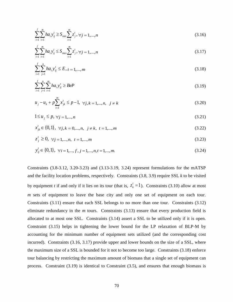
70

,zSyham

t

t

jmin

f

i

m

t

t

iji

11 1

n,...,j 1 (3.16)

,zSyham

t

t

jmax

f

i

m

t

t

iji

11 1

n,...,j 1 (3.17)

,Eyhaf

i

n

j

t

iji 1 1

mt ,...,1 (3.18)

BePyhaf

i

n

j

m

t

t

iji 1 1 1

(3.19)

,11

pxpuum

t

t

jkkj ,,...,1, nkj kj (3.20)

,1 pu j nj ,...,1 (3.21)

},1 ,0{t

jkx ,,...,0, nkj ,kj mt ,...,1 (3.22)

,0t

jz ,,...,1 nj mt ,...,1 (3.23)

},1 ,0{t

ijy

.,...,1,,...,1,,...,1 mtnjfi (3.24)

Constraints (3.8-3.12, 3.20-3.23) and (3.13-3.19, 3.24) represent formulations for the mATSP

and the facility location problems, respectively. Constraints (3.8, 3.9) require SSL k to be visited

by equipment t if and only if it lies on its tour (that is, 1t

kz ). Constraints (3.10) allow at most

m sets of equipment to leave the base city and only one set of equipment on each tour.

Constraints (3.11) ensure that each SSL belongs to no more than one tour. Constraints (3.12)

eliminate redundancy in the m tours. Constraints (3.13) ensure that every production field is

allocated to at most one SSL. Constraints (3.14) assert a SSL to be utilized only if it is open.

Constraint (3.15) helps in tightening the lower bound for the LP relaxation of BLP-M by

accounting for the minimum number of equipment sets utilized (and the corresponding cost

incurred). Constraints (3.16, 3.17) provide upper and lower bounds on the size of a SSL, where

the maximum size of a SSL is bounded for it not to become too large. Constraints (3.18) enforce

tour balancing by restricting the maximum amount of biomass that a single set of equipment can

process. Constraint (3.19) is identical to Constraint (3.5), and ensures that enough biomass is

71

utilized to satisfy the minimum processing capacity of the BcP. Constraints (3.20, 3.21) are the

extended version of the Miller, Tucker, and Zemlin (MTZ) subtour elimination constraints for

the multiple traveling salesmen problem presented by Kara and Bektas [77]. Constraints (3.22-

3.24) impose logical restrictions on the decision variables.

In the BLP-M formulation, the total cost to move equipment sets among the SSLs is relatively

smaller than the other costs in the model. Additionally, the modeling of the equipment

movement requires a large number of constraints, which heavily burdens the model. In an effort

to improve the solvability of the model, the problem is decomposed and solved in two stages.

The decomposed version of BLP-M is designated as BLP-MD. Stage 1 is solved using the BLP-

F model with a modification of the cost parameter ,M

js which now includes an estimated average

cost for moving the equipment from one SSL to another SSL. This results in a new objective

function (3.25).

f

i

n

j

ij

l

ij yd1 1

n

j

j

MD

j zs1

(3.25)

In addition, the following constraints are added:

,zSyha jmin

f

i

iji 1

n,...,j 1 (3.26)

,zSyha jmax

f

i

iji 1

n,...,j 1 (3.27)

Constraints (3.26) require the size of a SSL to be no smaller than 3 days of processing and

Constraints (3.27) establish an upper bound of 30 days of processing at a SSL. The latter also

replace Constraints (3.4). This results in the following first stage problem, designated as BLP-

MD1.

BLP-MD1: Minimize {3.25: 3.2-3.3, 3.5-3.6, 3.26, 3.27}.

The solution of BLP-MD1 specifies the values of y and z variables, i.e., the assignment of

production fields to SSLs, and the locations of SSLs. In Stage 2, the mATSP is solved to

72

determine the number of equipment sets to use and their routes over the SSLs. Objective

function (3.7) is modified by replacing with

and deleting the first term, to obtain:

Minimize

n

j

n

jkk

m

t

t

jkjk xc0 ,0 1

n

j

m

t

t

j

MD

j zs1 1

(3.28)

In addition, the following constraints are added:

,11

m

t

t

jz ,,...,1 nj (3.29)

,'1

Ezhan

j

t

jj

mt ,...,1 (3.30)

Clearly, Constraints (3.29) replace (3.11) thus requiring every selected SSL to be visited by a

tour. Constraints (3.30), similar to (3.18), track the biomass on a given tour to ensure that the

equipment can process the biomass within the allotted timeframe, noting that jha' is the amount

of biomass allocated to SSL j as determined by BLP-MD1. This leads to the following

formulation of mATSP for the second stage problem, designated as BLP-MD2.

BLP-MD2: Minimize {3.28: 3.8-3.10, 3.12, 3.15, 3.20-3.23, 3.29, 3.30}.

Next, an application of the above decomposed model formulation to a real-life scenario is

presented. The model formulations were solved directly using CPLEX 12.1.0 with OPL 6.3 on

an Intel Xeon E5335 2.00 GHz (8 thread) computer with 3.25 GB of RAM running Windows XP

SP3.

3.3. Results and discussion

In this section, results and relevant discussion are presented to compare: (1) the BLP-F, BLP-M,

and BLP-MD model formulations for the 13-km dataset with respect to the following criteria:

objective function value, number of SSLs opened, weighted average distance used for hauling

biomass, CPU time, and peak memory required, (2) different equipment systems along with their

permanent verse mobile options for the 32- and 48-km datasets in order to establish the best

strategy from the viewpoint of lowest objective function value and ease in implementing the

73

solution; and (3) the solutions obtained above with a heuristic solution that distributes SSLs

uniformly throughout the region. Also, a sensitivity analysis of parameter values is provided in

order to identify the operations that have the largest impact in reducing total cost.

3.3.1 Additional parameter setting

The equipment ownership cost is incorporated directly in the BLP-F model via the parameter ,

which represents the cost of opening SSL j, that is, the rental, development, and equipment costs.

For this study, a SSL land rental fee of $0.36/Mg [103] is used, assuming an identical cost for

each location; however, this cost could be location-dependent if land rental rates were to vary.

For the BLP-M model, the parameter represents the rental, development, and the

setup/takedown ($600 per move) cost for moving the mobile equipment to the next SSL being

unloaded. For BLP-MD1, the parameter includes an additional approximated cost

associated with moving the equipment to the next SSL; a distance of 8.5 km is used as an

approximation, resulting in a cost of $20. In BLP-MD2, this cost is calculated exactly and is

included in the final objective function value. The parameter, , captures the total cost incurred

for transporting the mobile equipment from SSL j to SSL k. The unit cost for travel between the

SSLs is assumed to be $2.29/km. The cost for owning the equipment is captured in parameter

for both BLP-M and BLP-MD2 models.

3.3.2 Comparison of model formulations

All three model formulations were solved using the 13-km dataset with the Side-loading Rack

System. This smaller dataset was utilized to enable the BLP-M formulation, the most

burdensome model, to solve to optimality. Table 3.1 provides the results for the three models

where the second column contains the total cost required to implement the logistics system, and

the sixth and seventh columns contain the weighted haul distance (km) per Mg.

Recall that the BLP-F model formulation assumes equipment sets to be placed permanently at

each and every SSL. This system has a higher cost for selecting SSLs due to the cost of

dedicated equipment, thereby selecting only one SSL, compared with 28 SSLs that are selected

for the mobile case, BLP-M, while still using only one set of equipment. The objective function

74

value for BLP-F is greater because of the longer haul distances from the production fields to the

SSL. The BLP-F model took 1.55 CPUs and required 18.29 MG to store the model.

Table 3.1: Comparison of model formulations Model/

Equipment system

Objective

function value

No. of Prod.

Fields

No. of

SSLS

No. of

Equip. Sets

Avg. dist.

to SSL (km)

Avg. dist.

to plant (km)

Comparison of model formulations: 13-km

BLP-F 1,067,903 118 1 1 11.01 2.63

BLP-M 916,032 119 28 1 1.68 10.71

BLP-MD 916,631 120 26 1 1.70 10.71

In both the BLP-M and BLP-MD formulations, the equipment was allowed to move from one

SSL to another. However, BLP-MD has been decomposed by first solving for the SSL locations,

and then, solving for the equipment tours over the SSLs. This solution methodology does not

guarantee attainment of optimal solutions. However, the results for the two mobile formulations

with respect to the number of production fields, SSLs, and equipment sets are nearly identical,

resulting in less than 1% difference in their objective function values. This reveals that the

proposed decomposition method is effective in finding near-optimal solutions. Furthermore, the

BLP-MD model required 0.92 CPUs and 18.76 MG of memory compared to 275.20 CPUs and

66.65 MG of memory for the BLP-M model. The additional time and memory is due to the fact

that the BLP-M model is formulated using all 31 potential SSLs. As a result of decomposition,

the BLP-MD2 formulation of BLP-MD requires only 26 selected SSLs, thereby reducing the size

and difficulty of solving the model.

3.3.3 Comparison of equipment systems

Comparisons among the use of different equipment systems as well as consideration of

permanent vs. mobile options are provided in order to establish the best strategy with respect to

the lowest objective function value. A comparison of the three different equipment systems to

perform operations at the SSLs and their respective costs are listed in detail in Table 3.2, where

the solution with the minimum total cost for each configuration is bolded for emphasis.

For the BLP-F models, the Side-loading Rack System resulted in the least cost solution. This is

mainly because of the reduced equipment cost when establishing a SSL for this system. This

reduction in setup cost justified the use of more SSLs than those for the Rear-loading Rack and

Densification Systems, thereby allowing shorter haul distances (2-3.5 km less) from the

75

production fields to the SSLs. The minimum feasible number of equipment sets possible is 6 and

12 for the 32- and 48-km datasets. Hence, since the Densification System achieved this bound, it

was most constrained by the cost of the SSLs. However, as additional equipment sets were

utilized for the rack systems, the cost of transporting biomass from the production fields to the

SSLs decreased. A graphical depiction of the 48-km solution is presented in Figure 3.1.

Table 3.2: Comparison of equipment systems Model/

Equipment system

Objective

function value

No. of Prod.

Fields

No. of

SSLS

No. of

Equip. Sets

Avg. dist.

to SSL (km)

Avg. dist.

to plant (km)

Comparison of equipment systems: 32-km

BLP-F

Side-loading Rack 5,848,497 714 10 10 8.01 21.33

Rear-loading Rack 6,614,986 721 7 7 9.96 19.18

Densification 7,479,742 709 6 6 10.34 20.84

BLP-MD

Side-loading Rack 4,938,672 680 141 6 1.84 24.07

Rear-loading Rack 5,647,218 668 142 6 1.84 24.77

Densification 6,452,506 644 144 6 1.76 24.71

Comparison of equipment systems: 48-km

BLP

Side-loading Rack 13,932,280 1644 24 24 7.61 34.21

Rear-loading Rack 15,687,437 1650 18 18 9.01 33.46

Densification 17,361,000 1704 12 12 11.03 33.87

BLP-MD

Side-loading Rack 11,815,138 1603 334 12 1.74 36.70

Rear-loading Rack 13,377,000 1589 335 12 1.74 36.73

Densification 14,792,773 1562 343 12 1.66 37.22

When utilizing mobile equipment on the larger-sized datasets, the BLP-MD2 model was found to

be much harder to solve. In order to solve the problem more efficiently, an advanced start

solution was provided by first solving the problem as a single TSP, and then, breaking this

solution into the minimum number of required tours. This solution helped in fathoming sub-

optimal solutions in the branch-and-bound process, and enabled CPLEX to solve the BLP-MD2

model to optimality for all instances.

By allowing the equipment to be moved from one SSL to another, the cost associated with the

development of a SSL was significantly reduced. A key point is to emphasize that the BLP-MD

models resulted in an increase in the number of SSLs required, thereby significantly reducing the

haul distance from the production fields to the SSLs. For all the models, the number of

equipment sets was no more than the minimum required for the respective dataset. As a result,

on average, each mobile equipment set visited 23.5 and 28 SSLs during the unloading operations

76

for the 32- and 48-km datasets, respectively. The average amount of load-haul duration at each

SSL varied from 10.4 to 12 days. It should be pointed out that the additional SSLs selected

allowed for shorter hauls from the production fields to the SSLs, thereby reducing this travel

distance by 6-9 km. The travel distance from the production field to the SSL is very significant.

A reduction in this distance reduced the total objective function value by an average of 14.8%.

In the 48-km dataset solution for the Side-loading Rack System, the minimum, average, and

maximum total production hectares assigned to a SSL are 30, 104, and 300, respectively.

Figure 3.1: Graphical depiction for the 48-km database using permanent equipment option

Although the Densification System affords a reduced cost in transportation, yet this benefit does

not outweigh the additional cost resulting from higher equipment operating costs at the SSLs,

specifically when compared with the Side-loading Rack System. The Side-loading Rack System

reduced the total cost by an average of 21.3%. Based on the cost data used, Densification should

only be utilized when the transportation distance is greater than 81 km, assuming that the

equipment is fully utilized at this distance on an identical set of SSLs. Additionally, the Rear-

loading Rack System gives no advantages over the Side-loading Rack System because of a

higher ownership and operating cost for the SSL equipment while providing no cost savings.

The calculated average total cost for delivery at the BcP using the 32- and 48-km datasets with

the Side-loading Rack System is 23.20 and 24.53 $/Mg. (This result was calculated by dividing

77

the objective function ($/year) by the annual capacity at the BcP (Mg/year).) This cost covers all

unit operations from retrieving the bales in the field to grinding operations at the BcP (not

including the cost to develop the receiving facility).

3.3.4 Comparison of the solutions obtained with a heuristic solution

A comparison of the solutions for the BLP-F and BLP-MD model formulations with a heuristic

solution presented in Resop et al. [118] is given for the 32- and 48-km datasets in Table 3.3. In

Resop et al. [118], a uniform distribution of SSLs throughout the study area was used by placing

the SSLs within 6.4 km (4 mi) of one another. All costs are calculated using the cost parameters

presented herein to ensure comparability of the solutions. For the “Optimal-fixed” formulation,

BLP-MD was solved with the addition of Constraint (3.31), which fixes the number of SSLs to

be the same as that used by Resop et al. (i.e. 99, 199 for the 32- and 48-km datasets,

respectively). This would highlight the difference in transportation cost resulting from the use of

optimal SSLs:

Rzn

j

j 1

(3.31)

The best solutions for the 32- and 48-km datasets from the comparison of equipment systems are

presented in bold in the table for comparison.

Table 3.3: Comparison of heuristic and optimal solutions Model/

Equipment system

Objective

function value

No. of Prod.

Fields

No. of

SSLS

No. of

Equip. Sets

Avg. dist.

to SSL (km)

Avg. dist.

to plant (km)

Comparison of heuristic and optimal solutions: 32-km

BLP-F

Resop solution 10,482,405 696 99 99 3.03 24.55

Optimal-fixed 10,010,873 673 99 99 2.21 23.74

BLP-MD

Resop solution 5,121,176 687 99 6 3.03 25.22

Optimal-fixed 4,955,667 673 99 6 2.21 23.74

Optimal 4,938,672 680 141 6 1.84 24.07

Comparison of heuristic and optimal solutions: 48-km

BLP-F

Resop solution 22,266,359 1635 196 196 3.33 37.18

Optimal-fixed 21,903,232 1606 196 196 2.35 36.38

BLP-MD

Resop solution 12,264,706 1635 196 12 3.33 37.18

Optimal-fixed 11,900,918 1606 196 12 2.35 36.38

Optimal 11,815,138 1603 334 12 1.74 36.70

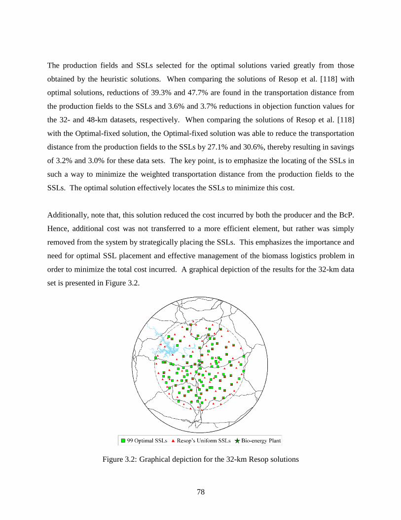
78

The production fields and SSLs selected for the optimal solutions varied greatly from those

obtained by the heuristic solutions. When comparing the solutions of Resop et al. [118] with

optimal solutions, reductions of 39.3% and 47.7% are found in the transportation distance from

the production fields to the SSLs and 3.6% and 3.7% reductions in objection function values for

the 32- and 48-km datasets, respectively. When comparing the solutions of Resop et al. [118]

with the Optimal-fixed solution, the Optimal-fixed solution was able to reduce the transportation

distance from the production fields to the SSLs by 27.1% and 30.6%, thereby resulting in savings

of 3.2% and 3.0% for these data sets. The key point, is to emphasize the locating of the SSLs in

such a way to minimize the weighted transportation distance from the production fields to the

SSLs. The optimal solution effectively locates the SSLs to minimize this cost.

Additionally, note that, this solution reduced the cost incurred by both the producer and the BcP.

Hence, additional cost was not transferred to a more efficient element, but rather was simply

removed from the system by strategically placing the SSLs. This emphasizes the importance and

need for optimal SSL placement and effective management of the biomass logistics problem in

order to minimize the total cost incurred. A graphical depiction of the results for the 32-km data

set is presented in Figure 3.2.

Figure 3.2: Graphical depiction for the 32-km Resop solutions

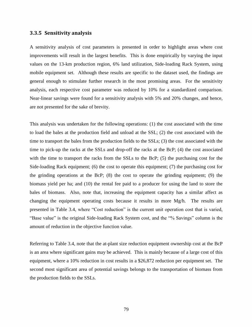
79

3.3.5 Sensitivity analysis

A sensitivity analysis of cost parameters is presented in order to highlight areas where cost

improvements will result in the largest benefits. This is done empirically by varying the input

values on the 13-km production region, 6% land utilization, Side-loading Rack System, using

mobile equipment set. Although these results are specific to the dataset used, the findings are

general enough to stimulate further research in the most promising areas. For the sensitivity

analysis, each respective cost parameter was reduced by 10% for a standardized comparison.

Near-linear savings were found for a sensitivity analysis with 5% and 20% changes, and hence,

are not presented for the sake of brevity.

This analysis was undertaken for the following operations: (1) the cost associated with the time

to load the bales at the production field and unload at the SSL; (2) the cost associated with the

time to transport the bales from the production fields to the SSLs; (3) the cost associated with the

time to pick-up the racks at the SSLs and drop-off the racks at the BcP; (4) the cost associated

with the time to transport the racks from the SSLs to the BcP; (5) the purchasing cost for the

Side-loading Rack equipment; (6) the cost to operate this equipment; (7) the purchasing cost for

the grinding operations at the BcP; (8) the cost to operate the grinding equipment; (9) the

biomass yield per ha; and (10) the rental fee paid to a producer for using the land to store the

bales of biomass. Also, note that, increasing the equipment capacity has a similar affect as

changing the equipment operating costs because it results in more Mg/h. The results are

presented in Table 3.4, where “Cost reduction” is the current unit operation cost that is varied,

“Base value” is the original Side-loading Rack System cost, and the “% Savings” column is the

amount of reduction in the objective function value.

Referring to Table 3.4, note that the at-plant size reduction equipment ownership cost at the BcP

is an area where significant gains may be achieved. This is mainly because of a large cost of this

equipment, where a 10% reduction in cost results in a $26,872 reduction per equipment set. The

second most significant area of potential savings belongs to the transportation of biomass from

the production fields to the SSLs.

80

Table 3.4: Sensitivity analysis of cost parameters

Cost Reduction Units Base value % Savings

1. Loading (unloading) at production field (SSL) $/Mg 3.35 0.42

2. Transport from the prod. field to SSL $/Mg/km 0.58 1.41

3. Loading (unloading) at SSL (BcP) $/Mg 1.66 0.69

4. Transport from the SSL to the BcP $/Mg/km 0.14 0.62

5. Side-loading Rack equipment ownership cost $/Equip. 55,011 0.59

6. Side-loading Rack equipment operating cost $/Mg 13.13 0.36

7. Grinding equipment ownership cost $/Equip. 268,723 2.93

8. Grinding equipment operating cost $/Mg/h 33.88 0.64

9. Yield Mg/ha 15.00 1.30

10. Storage cost $/Mg 0.36 0.15

This is because of the high cost per Mg per km, which emphasizes the importance of providing

SSLs closer to the producers in order for them to deliver their feedstock, and also, the value of

establishing better methods for transporting biomass from the production fields to the SSLs.

Finally, by increasing the yield (Mg/ha) of biomass, the total hectares required to meet a minimal

demand at the BcP are reduced, thereby decreasing the total travel distance. Note that, by

increasing the yield, the average travel distance from the production fields to the plant is reduced

by 0.4 km.

3.4. Concluding remarks

In this chapter, a feedstock logistics problem has been addressed that relies on the use of SSLs

and three possible equipment systems that are either placed permanently or are moved from one

SSL to another. It has been shown that: (1) small SSLs with mobile equipment result in savings

of 14.8%, (2) the Side-loading Rack System results in savings of 21.3% over the Densification

System, (3) when compared with a SSL location scenario presented in the literature, an optimal

SSL location scenario results in cost savings of 3%, and (4) the Densification System is not

justifiable for distances less than 81 km.

81

Chapter 4 Design, Model, and Analysis of a Feedstock Logistics System to Serve a Refinery

4. Hidden figure

Table 4: Hidden table

4.1. Introduction

In this chapter, we address a biomass logistics system that spans its operations from the

production fields to a refinery. Biomass is hauled from a set of predetermined production fields

to satellite storage locations (SSLs), which serve as common places for storage and subsequent

loading for highway hauling. From there, the biomass is thereby transported to one of several

small potential bio-crude plants (BcPs) where it is converted into bio-crude oil. This bio-crude

oil, a comparatively high-value product, is then, transported from the BcPs to a refinery for final

conversion and use as an energy product. The equipment required at a SSL is mobile, and can be

used to unload multiple SSLs. Plants that convert a cellulosic feedstock into a liquid fuel require

a large, complex logistics system where the number of truckloads of biomass varies between 50-

400 loads/day depending on the plant size and the conversion technology. As a result, an

industrial transportation system is introduced as early on in the system as possible.

The problem that we consider determines the optimal locations of the SSLs and the BcPs such

that the demand at the refinery is satisfied and the total cost accrued as a result of: (1)

transporting biomass from the production fields to the SSLs and from the SSLs to the BcPs, (2)

transporting bio-crude oil from the BcPs to the refinery, (3) moving the equipment among the

SSLs, and (4) for establishing the SSLs, is minimized. The locations of the production fields,

and the refinery, and the number of BcPs to be established are known a priori. This problem can

be viewed as a capacitated facility location problem with additional requirements, which stem

from the transportation of the mobile equipment among the SSLs, and consequently, give rise to

a multiple asymmetric traveling salesmen problem (mATSP). We formulate a mathematical

model for the underlying problem and propose a nested Benders’ decomposition-based

methodology for its solution.

The remainder of this paper is organized as follows. In Section 4.2, we present the biomass

logistics system in detail. This is followed by a formal definition of the biomass logistics

82

problem (BLP), and a literature review and formulation of a mathematical model for this

problem. We, then, present a nested Benders’ decomposition-based methodology for the

solution of the BLP. Computational results on the performances of the model formulations of

BLP by CPLEX 12.1.0 and nested Benders’ decomposition-based methodology are presented in

Section 4.5 by utilizing five randomly-generated datasets that emulate a real-life scenario in the

Southeastern United States. Finally, concluding remarks and suggestions for future research are

presented in Section 4.6.

4.2. Biomass logistics system

The cost incurred for transporting biomass from the production fields until its conversion to an

energy product at a refinery is known to constitute a large portion of the total cost of biofuel

production. As much as 35-60% of the total price of ethanol biofuel at the gas pump is

associated with the transportation cost [40, 79, 147]. It is, therefore, essential that this

transportation cost is curtailed as much as possible to enable biofuel to be an attractive

alternative source of energy. Much of the high transportation cost results from the fact that raw

biomass has a relatively low haul-density (Mg/m3). Additionally, the equipment designed for

hauling biomass in the field is inefficient on the roadways as compared with the use of tractor-

trailer trucks.

It is for this purpose that we propose the use of satellite storage locations (SSLs), distributed

throughout the production region (see Figure 4.1 for an illustration) [22, 24, 141]. The locations

of the SSLs are determined so as to minimize the total cost incurred for handling (loading,

transport cost and unloading into storage) of biomass from the production fields to the SSLs plus

the development of the SSLs.

A specialized loading equipment set is designed to be mobile. This permits the equipment to

move from one SSL to another SSL as each is emptied, thereby increasing the productivity of the

equipment and making it possible to justify a reduction in the coverage area for each SSL, since

the loading equipment can still be fully utilized to unload multiple SSLs [74]. Within each

BcP’s geographic coverage area, it is necessary to use multiple sets of equipment in order to

provide enough biomass at the plant. The unloading of SSLs with multiple sets of equipment

83

gives rise to a multiple asymmetric traveling salesmen problem (mATSP), which must be solved

for each BcP. Additionally, the workload of each set of equipment must not exceed its total

capacity. The details for implementing the logistics system from the production field to the BcP

and the respective costs that we utilize in an analysis are presented in Chapter 2. A synopsis of

these costs is presented in Table 4.1 noting that these costs do not include the labor, which is

assumed to be $20/h.

Figure 4.1: Sample area of production fields and potential satellite storage locations (SSLs)

The optimal locations for the BcPs must be determined from a set of potential sites. Enough

biomass must be allocated to each BcP to ensure continuous production throughout the year.

These BcPs are built to the smallest economically feasible size. The purpose of this small size is

to reduce the total distance traveled by the biomass. The locating of the SSLs and BcPs results

in a two-level facility location problem [89].

At a BcP, the biomass is processed into pyrolitic oil (hereby referred to as bio-crude oil) at a rate

of 510 l/Mg at 22,300 KJ/l [97] by heating the biomass to approximately for a few

seconds in the absence of oxygen. Once converted into bio-crude oil, the energy density is

greatly increased, thereby justifying a long transportation distance to a refinery for final

processing and blending.

84

Table 4.1: Equipment specifications for operations performed at a satellite storage location

Equipment systems Purchase

price ($)

Design life

(h)

R/Ma factor

($/h)

Fuel use

(L/h)

Equip.

cap. (Mg/h)

Equip. own.

cost ($/yr.)

Total Equip.

op. cost ($/h)

Side-loading Rack System

Telehandlerb 88,000 10,000 2.00 7.5 21.6 27,790 9.65

Drop-deck trailer (2) 60,000 5 y 15%c - 14.4

d 16,107

e 3.19

Rack (8) 41,400 5 y 2%c - 7.2

d 11,114 0.29

Total

55,011 13.13

At-plant size reduction

Tub-grinder

377,500 15,000 1.43 - 22.7 202,249 1.43

Electric motor 123,400 15 y 3%c

400.0f

22.7 16,638e

26.91

Dust control tech. 200,000 5 y 6%c

20.0f

22.7 53,691e 5.54

Total

268,723 33.88 a:

b:

c:

d:

e:

f:

Repair and maintenance

Personal contact with Ted Mallard, American Equipment Service Inc., 1888 Sabina Road Wilmington Ohio, 45177

The maintenance cost is a percentage of the purchase price, applied at an hourly cost assuming 2820 operating h/yr.

The units for the equipment capacity are Mg/rack and Mg/trailer

Calculated using a Capital Recovery Factor (CRF) plus tax rate = 1% and insurance = 0.8%

Energy use in kW-h, we assume $0.08/kW-h and a duty factor of 0.8

Once the biomass has been converted into bio-crude oil at a BcP, it is temporarily stored in large

storage tanks in preparation for the next delivery. A detailed analysis of the equipment and

structural cost for receiving at a BcP is provided in Table 4.2 in addition to the cost to transport

bio-crude oil to the refinery.

For transporting bio-crude oil, we consider a rail network with railcars. This system is attractive

when there is a long transportation distance between the BcPs and the refinery. For this option,

we assume that the BcPs are located on a rail-network, thereby constraining the locations of the

BcPs along the rail network.

The cost to transport full (and then empty) cars to and from the refinery is estimated using a

fixed cost of $1232.9 per car and a variable cost of $5.2944 per km per car. (Estimated from

communication with Tom Landrum at N&S Railroad.) Once at the refinery, the bio-crude is

further refined through a deoxygenating process for direct use and is, thus, upgraded to be

blended with petroleum fuel. Sixty-seven percent of the bio-crude is refined during this process,

and the remaining residues have other applications [12, 14, 113]. The components are then

blended, stored, and shipped for final use.

85

Table 4.2: Cost analysis for loading at a bio-crude plant

Equipment systems Purchase

price ($)

Design life (h) R/M factora

($)

Energy use Own.

Costb ($/yr.)

Total op. costc ($)

Storage tanks 450,000 20 yrs. 7,250/yr. 75/kW-hd 46,110 229,346/yr.

Yard Engine 430,000 20 yrs. 12.00/h 15.14 L/he 35,432 48.00/hf

Individual Railcar Rental 9,600/yr. 9,773g a: b:

c: d:

e:

f: g:

Repair and maintenance factor The equipment ownership cost is calculated using ASABE Standard ASAE EP496.3 FEB2006, assuming: salvage value = 10%, interest

rate = 8%, tax rate = 1%, and insurance = 0.8%

Total Operating Cost = Repair and maintenance + Energy use + Labor (at $20/h) Energy use in kW-h, we assume $0.08/kW-h and a duty factor of 0.8

We assume the cost of diesel fuel is $1.06/L ($4/gal.)

The Yard engine’s equipment utilization is conservatively assumed to be 1 car/h Including taxes (1%) and insurance (0.8%)

For our analysis, we have considered the costs incurred starting from the bales sitting in the field

until the bio-crude oil is received at the refinery. However, because of a high variability in the

cost of building a BcP, we have not included the cost incurred for the conversion of biomass into

bio-crude oil, which comprises the costs incurred starting from the time after the biomass has

been ground at the BcP until it has been processed and pumped into temporary storage at the

BcP. We have included the cost to develop the storage tank and rail siding at the BcP since these

costs are well-defined by industry.

4.3. Problem definition, literature review, and model formulation

The biomass logistics problem (BLP) that we address in this chapter has been introduced

previously, and can be concisely stated as follows: Given f potential production fields and a set

of n potential locations for SSLs, determine the optimal number of production fields and SSLs,

the placement of SSLs (production fields on which to build the satellite storage facilities), and

the allocation of production fields to SSLs. Additionally, determine the optimal locations of the

BcPs from a set of predetermined candidate locations so as to minimize the total cost incurred

for transporting: (1) biomass from each production field to a SSL, (2) biomass from SSLs to the

BcP, and (3) bio-crude oil from the BcPs to the refinery, and moreover, determine the minimal-

cost of routing of the mobile equipment among the SSLs.

As described in Section 4.2, each SSL must be visited by a set of loading equipment. The

equipment routing problem is similar to the multiple asymmetric traveling salesmen problem

(mATSP), which can be stated as follows: Given a set of n potential SSLs (cities) and m

equipment sets (traveling salesmen), determine m tours, one for each set of equipment, such that,

86

starting from a reference base (SSL facility), each equipment set visits a subset of the SSLs and

returns to the base SSL facility, each SSL is visited by exactly one equipment set, and the total

distance traveled by all the equipment sets is minimized.

The transportation of biomass from the production fields to the SSLs on the way to the BcPs and

eventually to the refinery can be classified as a 2-level facility location problem. The two levels

pertain to the locations of SSLs and the BcPs. The single-level and k-level facility location

problems have been addressed in the literature [89]. For the single-level facility location

problem, Erlenkotter [38] has proposed an effective dual-based method that has been applied to

solve relatively large-sized problems. A review of work for this problem can be found in [94,

98, 109]. For work on the more general k-level facility location problem, see [112, 119, 151].

Research reported in the biomass logistics area can be divided into two types of variables

depending upon the environment encountered: stochastic or deterministic, and integer or

continuous. In the areas of stochastic and deterministic environment, Kumar and Sokhansanj

[84] have presented an integrated biomass supply analysis and logistics model, which captures

the stochastic bio-crude logistics issues. Additional work in this area can be found in [28, 51,

106, 117]. In the deterministic environment, most of the reported work utilizes a geographic

information system (GIS) interactively with an optimization solver. This allows the GIS package

to work as a data management tool, which may call the optimization software directly. Most of

the deterministic models presented are mixed-integer programs [50, 93, 141, 142]. The proposed

BLP model is a deterministic model that also utilizes GIS for data management. However, our

BLP model is different because of the inclusion of SSLs for local storage and use of mobile

equipment to unload a series of SSLs.

When the given environment is modeled using continuous variables, the entire land within a

region is utilized for biomass production [52, 103, 104]. It leads to simple calculations, and it

avoids the details required to help a decision maker implement a specific strategy. In the BLP

model, each production field is considered as a specific entity with specific costs, which

introduces integer variables, a more detailed representation, and a direct solution to the problem.

87

In a recent work published by Zhu et al. [154], a model is presented that is similar in many ways

to the work presented herein, but they assume a single predetermined BcP. Their formulation

effectively models much of the operations that need to take place in the logistics system for a

given BcP. Moreover, the formulation presented by Zhu et al. [154] is too complex, requiring

the data used as inputs to be overly aggregated in order to keep the model’s size reasonable. In

the work of Shastri et al. [126], a general model is used that relies on data aggregation at the

county level. In the formulations of large-sized problems, it is prudent to provide a balance

between the amount of detail captured in the model and the amount of detail provided by the

data. This is because the main bottleneck is the available RAM of the computer. Our BLP

model is developed with this view in mind.

Consider the following notation:

Parameters:

f Number of production fields

n Number of potential locations for a SSL

b Number of locations for potential BcPs

m Maximum number of mobile equipment sets

ijld Unit cost to transport the biomass from production field i to the refinery through SSL j

and BcP l, blnjfi ,...,1,,...,1,,...,1

jkc Unit cost to move the mobile from SSL j to SSL k, kjnkj ,,...,0, where j, k = 0

represent a dummy SSL, and kc0 and 0jc represent dummy costs

js Rental/development fee for utilizing SSL j (paid to the production field owner),

nj ,...,1

iha Size of production field i (in hectares), fi ,...,1

mins

Minimum allowable size of a SSL (3 days worth of unloading in hectares)

maxs

Maximum allowable size of a SSL (30 days worth of unloading in hectares)

Q Number of BcPs required

E Maximum processing capacity for each mobile equipment set (in hectares)

BcP Minimum processing capacity for each BcP (in hectares)

R Minimum processing capacity for the refinery (in hectares)

88

We assume that the cost of a moving equipment is much greater than the cost incurred during its

movement among the SSLs, which generally holds true in practice.

Decision Variables:

,0

,1t

ijly

if production field i transports biomass to SSL j on the way to BcP l on

mobile equipment tour t

otherwise, blnjfi ,...,1,,...,1,,...,1

,0

,1t

jklx

if SSL j directly precedes SSL k, on mobile equipment tour t, for BcP l

otherwise, blmtkjnkj ,...,1,,...,1,,,...,0,

,0

,1t

jlz

if SSL j is allocated to BcP l and visited on mobile equipment tour t

otherwise, ,,...,0 nj mt ,...,1

,0

,1lq

if BcP l is utilized

otherwise, bl ,...,1

iu a rank order index associated with city i, .,...,1 ni

Intuitively, t

ijly represents the transportation of biomass from a production field i to SSL j, on

tour t, which is then transported to BcP l. The variables ,,t

jl

t

jk zx and iu are used to capture the

tour of each equipment and to generate subtour elimination constraints.

We have the following formulation:

BLP-MTZ: Minimize

b

l

n

j

n

jkk

m

t

t

jkljk xc1 0 ,0 1

+

f

i

n

j

b

l

m

t

t

ijlijl yd1 1 1 1

b

l

n

j

m

t

t

jlj zs1 1 1

(4.1)

subject to:

,,0

t

kl

n

kjj

t

jkl zx

,,...,0 nk ,,...,1 mt bl ,...,1

(4.2)

,,0

t

kl

n

kjj

t

kjl zx

,,...,0 nk ,,...,1 mt bl ,...,1

(4.3)

,11

0

b

l

t

lz ;,...,1 mt

(4.4)

89

m

t

t

lz1

0 ⌈ ⁄ ⌉ bl ,...,1

(4.5)

,min( 1

nzn

j

t

jl

⌈ ⁄ ⌉

,,...,1 mt bl ,...,1

(4.6)

, 0

1

t

l

n

j

t

jl zz

,,...,1 mt bl ,...,1

(4.7)

,11 1

b

l

m

t

t

klz nk ,...,1

(4.8)

,11 1 1

n

j

b

l

m

t

t

ijly fi ,...,1

(4.9)

,t

jl

t

ijl zy ,,...,1,,...,1 njfi ,,...,1 mt bl ,...,1

(4.10)

,1

l

m

t

t

jl qz

,,...,1 nj bl ,...,1

(4.11)

Qqb

l

l 1

(4.12)

,1 1

min

1 1 1

b

l

m

t

t

jl

f

i

b

l

m

t

t

ijli zsyha nj ,...,1

(4.13)

,1 1

max

1 1 1

b

l

m

t

t

jl

f

i

b

l

m

t

t

ijli zsyha n,...,j 1

(4.14)

,1 1 1

Eyhaf

i

n

j

b

l

t

ijli

mt ,...,1

(4.15)

, 1 1 1

l

f

i

n

j

m

t

t

ijli qBcPyha

bl ,...,1

(4.16)

Ryhaf

i

n

j

b

l

m

t

t

ijli 1 1 1 1

(4.17)

b

l

m

t

t

l

1 1

0z ⌈ ⌉ (4.18)

,1

1

0

1

0

b

l

t

l

b

l

t

l lzlz 1,...,1 mt (4.19)

,11

nxnuub

l

t

jkl

t

k

t

j ,,...,1, nkj ,kj mt ,...,1

(4.20)

90

,01 1

b

l

n

k

t

kl

t

j zu ,,...,1 nj mt ,...,1

(4.21)

},1 ,0{t

jklx ,,...,0, nkj ,kj ,,...,1 mt bl ,...,1 (4.22)

},1,0{t

jlz ,,...,0 nj ,,...,1 mt bl ,...,1 (4.23)

,0t

ijly

,,...,1,,...,1 njfi ,,...,1 mt bl ,...,1 (4.24)

},1,0{lq .,...,1 bl (4.25)

Constraints (4.2-4.8, 4.18-4.23) and (4.9-4.17, 4.24, 4.25) represent formulations for the mATSP

and the facility location problem, respectively. Constraints (4.2) and (4.3) require SSL k

allocated to BcP l to be visited by equipment t if and only if it lies on its tour (when 1t

klz ).

Constraints (4.4) ensure that at most one BcP can belong to a tour, while Constraints (4.5, 4.6,

4.7) tighten the LP relaxation of the t

lz0 -variables. Constraints (4.8) ensure that each SSL is

assigned to at most one BcP and equipment set, while Constraints (4.9) assert that each

production field is allocated to at most one SSL, equipment set, and BcP. Constraints (4.10) and

(4.11) ensure that a SSL and a BcP are only utilized if they are open. Constraint (4.12) ensures

that Q BcPs are opened to satisfy the demand at the refinery. The number of BcPs is fixed

because of the high variability in the estimated cost to build a production-scale BcP. Note that

the locations of Q BcPs are selected from b potential locations. The cost of building a BcP is

assumed to be identical at all locations. Constraints (4.13-4.17) are feasibility constraints for the

given problem. Constraints (4.13) and (4.14) provide a lower and an upper bound, respectively,

on the size of each SSL. Constraints (4.15) ensure that each equipment set’s capacity is not

exceeded. Constraints (4.16) and (4.17) assert that the minimum processing capacity at the BcPs

and refinery, respectively, are satisfied. Constraint (4.18) tightens the lower bound for the LP

relaxation by accounting for the lower bound on the number of equipment sets. Constraints

(4.19) constitute symmetry breaking constraints for the m tours. Constraints (4.20) and (4.21)

are subtour elimination constraints as suggested by Miller, Tucker, and Zemlin (MTZ),

subsequently, extended by Kara and Bektas [77] for the multiple traveling salesmen problem,

and extended by Sarin et al. [121]. These constraints, although lacking in the tightness of the

linear relaxation prove to be quite effective due to the simplicity of their formulation. Constraint

sets (4.22-4.25) impose logical restrictions on the decision variables.

91

We additionally assume that each production field can only transport to a potential SSL that is

relatively close to it. Because of the high cost of transporting biomass from the production fields

in relation to the cost of developing a SSL, the number of variables in the formulation can be

significantly reduced by fixing variables to zero if the distance from production field i to SSL j is

relatively large.

4.4. Solution methodology via nested Benders’ decomposition

In Benders’ decomposition, a series of master and sub-problems are solved iteratively [10]. This

enables solution of large-sized problems as the master problem and sub-problems are smaller in

size as compared with the size of the original problem. The master problem is a relaxation of the

original formulation obtained by removing some constraints, and is solved to obtain an initial

solution. A sub-problem that typically represents the dual, or pricing, of the relaxed constraints is

solved to generate a new Benders’ cut if the current master problem solution is violated [102].

This constraint is added to the master problem, and is then re-solved. This process is continued

until the master problem and sub-problem converge to an optimal solution.

We further exploit this approach by solving the sub-problem itself via Benders’ decomposition.

This results in nested Benders’ decomposition, which was first introduced for stochastic

problems by Birge [11], and which has been successfully applied to many multistage stochastic

problems (see [3, 53, 95]). To the best of our knowledge, this approach, however, has not been

applied to deterministic problems.

Consider the following result:

Proposition 1: The use of Benders’ decomposition in the sub-problem of a problem that has

already been decomposed using Benders’ decomposition is a legitimate decomposition scheme

that leads to a globally optimal solution to the non-decomposed problem.

Proof. The essence of Benders’ decomposition is to obtain a Benders’ cut by solving the sub-

problem to optimality and add it to the master problem in order to cut off the current master

92

problem solution or validate optimality. Hence, it is necessary that the sub-problem does indeed

converge to the optimal solution and generates a valid cut (via the dual solution value) for the

master problem. The sub-problem solved using classical Benders’ decomposition technique

does, in fact, converge to the optimal solution under normal conditions, whence, the dual values

(which are readily available) generate a valid cut for the master problem.

It is for these reasons that a decomposed model is proposed by removing from the master

problem the allocation of production fields to SSLs, equipment sets, and BcPs (y-variables) and

the mATSP formulation (x-variables). We designate the nested Benders’ decomposition based

on the formulation BLP as BLP-B. The SSLs and BcPs are selected in the master problem

(BLP-MP), while the allocation of production fields to SSLs, equipment sets, and BcPs (y-

variables), and the mATSP (x-variables) are relegated to the sub-problem. We designate this

nested Benders’ decomposition as BLP-B. Since the sub-problem is also solved using Benders’

decomposition, the decomposition scheme results in three parts, namely, BLP-MP (master

problem), BLP-SP1 (sub-problem for BLP-MP), and BLP-SP2 (sub-problem for BLP-SP1). In

the first sub-problem (BLP-SP1), the production fields (y-variables) are allocated to SSLs (z-

variables), and additionally, the SSLs are allocated to equipment sets. This information is passed

to the second sub-problem (BLP-SP2) that is decomposable into independent problems

corresponding to each of the set of mobile equipment allocated to each BcP, and it determines an

ATSP tour for each mobile equipment. The advantage of this formulation over solving the sub-

problem without decomposition is that the non-decomposed sub-problem would require the

solution to a very large mATSP, which would restrict solution to only small-sized problems.

However, smaller ATSPs, obtained via decomposition, are easier to solve, which allows for the

solution of large-sized problems. The master problem is formulated as follows:

BLP-MP: Minimize

b

l

n

j

jlj zs1 1

objz

(4.26)

subject to:

,11

b

l

klz nk ,...,1

(4.27)

,ljl qz ,,...,1 nj bl ,...,1

(4.28)

93

Qqb

l

l 1

(4.29)

, l

1

max qBcPzsn

j

jl

bl ,...,1

(4.30)

Rzsb

l

n

j

jl 1 1

max

(4.31)

},1,0{jlz ,,...,1 nj bl ,...,1

(4.32)

},1,0{lq bl ,...,1

(4.33)

.0objz

(4.34)

Constraints (4.27, 4.28, 4.30-4.32) are aggregations of Constraints (4.8, 4.11, 4.16, 4.17, 4.23)

where .1

jl

m

t

t

jl zz

These constraints ensure the proper modeling of the z- and q-variables.

Constraints (4.30) and (4.31) provide an initial bound on the minimum total number of SSLs

required for each open BcP and for the entire system, respectively. These constraints help to

ensure that BLP-MP is more likely to provide a feasible solution to BLP-SP1.

Benders’ cuts are added to the BLP-MP as they are generated. We present these cuts after the

formulation of the sub-problems. As noted earlier, the sub-problem is solved via another

Benders’ decomposition. The first sub-problem that allocates production fields to SSLs and

SSLs to tours is as follows:

BLP-SP1: Minimize

f

i

n

j

b

l

m

t

t

ijlijl yd1 1 1 1

tspz (4.35)

subject to:

,1

jl

m

t

t

jl zz

,,...,1 nj bl ,...,1 )(

(4.36)

,11

0

b

l

t

lz mt ,...,1 )(

(4.37)

m

t

t

lz1

0 ⌈ ⁄ ⌉ bl ,...,1 )(

(4.38)

94

,min( 1

nzn

j

t

jl

⌈ ⁄ ⌉

,,...,1 mt bl ,...,1

(4.39)

, 0

1

t

l

n

j

t

jl zz

,,...,1 mt bl ,...,1

(4.40)

,11 1 1

n

j

b

l

m

t

t

ijly fi ,...,1 )(

(4.41)

,t

jl

t

ijl zy ,,...,1 fi ,,...,1 nj ,,...,1 mt bl ,...,1

(4.42)

,1

min

1 1 1

b

l

jl

b

l

m

t

f

i

t

ijli zsyha nj ,...,1 )(

(4.43)

,1

max

1 1 1

b

l

jl

b

l

m

t

f

i

t

ijli zsyha nj ,...,1 )(

(4.44)

,1 1 1

Eyhaf

i

n

j

l

l

t

ijli

mt ,...,1 )(

(4.45)

, 1 1 1

l

f

i

n

j

m

t

t

ijli qBcPyha

bl ,...,1

)(

(4.46)

Ryhaf

i

n

j

b

l

m

t

t

ijli 1 1 1 1

)(

(4.47)

REb

l

m

t

t

l 1 1

0z )( (4.48)

,1

1

0

1

0

b

l

t

l

b

l

t

l lzlz 1,...,1 mt

(4.49)

,0t

ijly ,,...,1,,...,1 njfi ,,...,1 mt bl ,...,1

(4.50)

0tspz

(4.51)

},1,0{t

jlz ,,...,1 nj ,,...,1 mt bl ,...,1

(4.52)

Constraints (4.36) are the linking constraints between the master problem and the sub-problems.

Constraints (4.37-4.40) are those in the original non-decomposed problem, BLP-MTZ. Given a

solution to BLP-SP1, BLP-SP2 is decomposable into sub-problems, one for each of the

equipment tours associated with a BcP (l). For each tour t associated with a BcP the formulation

of BLP-SP2 is as follows:

95

BLP-SP2l t: Minimize

n

j

n

jkk

t

jkljk xc0 ,0

(4.53)

subject to:

,,0

t

kl

n

kjj

t

jkl zx

nk ,...,0 )(

(4.54)

,,0

t

kl

n

kjj

t

kjl zx

nk ,...,0 )(

(4.55)

,1 nnxuu t

jkl

t

k

t

j ,,...,1, nkj ,kj mt ,...,1 )( (4.56)

,1 1

b

l

n

k

t

kl

t

j zu ,,...,1 nj mt ,...,1 )(

(4.57)

,0t

ju ,,...,1 nj mt ,...,1

(4.58)

,0t

jklx ,,...,0, nkj kj

(4.59)

The constraints for BLP-SP2 t

l emulate Constraints (4.20-4.23) of BLP-MTZ where the -

variables are now fixed as inputs. However, in order to ensure that Constraints (4.54) and (4.55)

remain feasible to BLP-SP2 t

l, the

-variables must be binary, while BLP-SP1 is solved as an

LP, and there is no guarantee that they will indeed assume binary values as a result.

In order to generate a valid solution for BLP-SP2 for our solution procedure, we convert the LP

solution generated for the sub-problem (BLP-SP1) into an integer solution as follows. The

partitioning of the -variables is a result of constraints (4.45), which limit the allocation of

biomass to a tour. Hence, generally, there will be only 2m variables that are not binary. The

underlying problem can be viewed as a bin packing problem with bins of limited capacity. In

our case, mobile equipment constitutes a bin and the SSLs the items to be placed in that bin, and

Constraints (4.45) are the capacity constraints for the bins. This bin packing problem is naturally

decomposable among the l BcPs since, for a given solution of BLP-MP (which allocates SSLs to

BcPs), the SSLs can only be reallocated to mobile equipment sets within the same BcP. As a

result of this re-allocation, note that, feasibility of the LP bound constraints (4.37), (4.38), and

(4.49) is maintained since the -variables remain unchanged. Feasibility constraints (4.43-4.44,

4.46-4.48) remain unchanged since they do not distinguish between tours. Moreover, next, we

96

show that the solution of the bin packing problem, as described above, results in a feasible

solution to BLP-SP1.

Corollary 1. The number of sets of equipment used in the LP solution of BLP-SP1 constitute a

lower bound on the number of sets of equipment used in the integer problem.

Proof. A variable z is said to dominate a set of variables in a model that are affected by z if the

potential savings (cost) from the affected variables are overridden by the cost (savings) of the z-

variables. For this model, the -variables (selecting the number of tours) dominate the x-

variables (the paths of the tours) because any savings achieved by reconfiguring the x-variables

as a result of an additional equipment set, would never outweigh the additional cost of the

equipment set, by assumption. Hence, the model will always use the least number of equipment

sets possible in the LP solution.

Proposition 2. For a given BcP, re-allocating SSLs to different mobile equipment sets always

results in a feasible solution to BLP-SP1 if constraint (4.45) is not violated.

Proof. Note that only Constraints (4.39), (4.40), and (4.42) are affected as a result of the re-

allocation of SSLs to different equipment sets for a given BcP.

Constraints (4.45) ensures that the capacity, E, of each equipment is not violated. In view of the

maintenance of the minimal size of the SSL, by Constraints (4.43), remains

unchanged in (4.39). Hence, the maximum number of SSLs allowed on a tour will never be

more than n or when all the SSLs are as small as possible, ⌈ ⌉. Therefore, Constraints

(4.39) will not be violated.

Constraint (4.40) ensures that if the -variable is one, then at least one SSL is allocated to the

tour. As long as one SSL remains in a tour, constraint (4.40) will remain feasible. If it were

possible to remove all the SSLs from a tour, then this tour could be removed. However, if a tour

is removed from the integer solution, then it would result in a better objective function value.

This implies that it could be removed from the LP solution as well in order to obtain a better

97

solution. But this contradicts the fact that the current LP solution is optimal by Corollary 1.

Therefore, all the tours must contain at least one SSL in them. Thus, constraint (4.40) will not be

violated.

Constraint (4.42) is simply adjusted to account for the new equipment assignment. This affects

Constraint (4.45) to ensure that the proper amount of biomass is allocated to the tour. The

feasibility of Constraint (4.45) is maintained in the bin packing problem.

This provides a method to obtain an integer solution by re-allocating the SSLs among the mobile

equipment sets belonging to a BcP. If a feasible solution exists, then we can use it for BLP-SPl t.

Otherwise, it implies that the current solution obtained for BLP-SP1 is infeasible and it does

not utilize sufficient mobile equipment sets for at least one BcP. We include the following

constraint that specifies an additional mobile equipment for each infeasible BcP solution:

,1 1

0

l

m

t

t

l NESz

(4.60)

where NESl is the number of mobile equipment sets for BcP l utilized in the sub-problem

solution. When needed, this constraint is added to BLP-SP1, and BLP-SP1 is re-solved.

However, our experience with empirical data has revealed that the LP solution from BLP-SP1 is

typically not constrained enough to require the solution of the l bin packing problems formally.

For simplicity, we exploit a greedy heuristic because of its success in generating good solutions,

while also resulting in a solution that is very similar to the LP solution. To that end, we allocate

-variables to the tour with the highest LP solution value. If this solution is not feasible, then

the l bin packing problems must be solved to optimality.

This solution is used as an input to BLP-SP2l t, whereupon after its solution, a cut is sent to BLP-

SP1. BLP-SP1 is subsequently re-solved and the process is continued until an optimal solution

has been found for the complete sub-problem. A cut is then generated for BLP-MP, and the

master problem is thereby re-solved. The cuts that are added iteratively after the solution to each

sub-problem are as follows:

98

b

l

n

j

jljjjl

m

t

tt

f

i

iobj zssREz1 1

maxmin

11

)() ()(

b

l

n

k

n

kjj

jklll nqE

BcPBcP

1 1 :1

,)1()( (4.61)

,)1()(1 1 1 11 ;11 1 0

b

l

m

t

n

j

n

k

t

kl

t

jl

n

k

n

kjj

jk

b

l

m

t

n

j

t

jl

t

jl

t

jltsp znzz

(4.62)

In the event that the current master problem solution results in infeasibility for BLP-SP1, we use

the following cut that ensures that the current master problem solution is not used again:

,1101 ,,,

Zlj

jl

Zlj

jl

Zlj

jl zzz

(4.63)

where 1Z and 0Z represent indices of the z-variables that were equal to one and zero,

respectively, in the prior master problem solution. We prove this next.

Proposition 3. Constraint (4.63) eliminates only the current solution and is a valid cut for the

master problem.

Proof. We prove this proposition via induction on the number of z-variables, where the indices

of z are reduced to a single index for simplicity. If , then there is only one feasible solution

to the master problem, and hence, this constraint would never be implemented. If , then

there are 3 trivial cases to be considered. If there are no variables currently being utilized, then

only preventing the current solution. If there is one variable currently being utilized

(we arbitrarily assume ), then Clearly, this constraint does not permit the

current solution and . And lastly, when both variables are currently being utilized,

we have which does not permit the current solution, , .

Now, assuming that the result holds true for n, that is, ,01)(001

Zi

i

Zj

j

Zi

i zzznS we

need to show that it holds true for . Consider the following.

99

Case 1: in the master problem. We have

.0)(1

011

01)1(

1

1:

1

001

001

nSz

zzzz

zzznS

n

Zi

i

Zj

j

niZi

in

Zi

i

Zj

j

Zi

i

(4.64)

We want to show that after constraint (4.64) is added to the master problem, and it is re-solved,

when )(nS is the same as before. Suppose that in this new solution of the master

problem, and )(nS is the same as before. By (4.64), .0)()1( nSnS By induction,

)(nS is infeasible if the new solution for the n z-variables is the same as before, in a feasible

solution to the master problem when )(nS is the same as before.

On the other hand, if after adding Constraint (4.64) to the master problem, we want to

show that the new solution of the master problem is feasible. By (4.64), ,01)()1( nSnS

or ,1)( nS which implies that all feasible solutions for )(nS still remain feasible since by

induction .0)( nS

Case 2: We assume that in the master problem. For this case, we note that,

.0)(

01

01)1(

1

1:1:

1

001

001

nSz

zzzz

zzznS

n

niZi

i

njZj

j

Zi

in

Zi

i

Zj

j

Zi

i

(4.65)

We want to show that after (4.65) is added to the master problem, and it is re-solved,

when )(nS is the same as before. Suppose that in this new solution of the master problem,

and )(nS is the same as before. By (4.65), .0)()1( nSnS By induction, )(nS is

infeasible if the new solution for the n z-variables is the same as before, which contradicts the

fact that in a feasible solution to the master problem when )(nS is the same as before.

100

On the other hand, if after adding Constraint (4.65) to the master problem, we want to

show that the new solution of the master problem is feasible. By (4.65), ,01)()1( nSnS

or ,1)( nS which implies that all feasible solutions for )(nS still remain feasible since by

induction .0)( nS

4.5. Application to a potential real-life scenario

In this section, we present results of our computational investigation conducted to compare

performances of direct solution of BLP by CPLEX with the nested Benders’ decomposition-

based method, BLP-B. We utilize randomly generated data that has been developed to emulate a

real-life scenario in the Piedmont region of the Southeastern United States. The computations

were performed using CPLEX 12.1.0 with OPL 6.3 on an Intel Duo Core E5335 2.00 GHz

computer with 3 GB of RAM running Windows Vista.

We generated five datasets, for each of which, random points were generated using a uniform

distribution to represent the production fields. The locations of these production fields were

required to be within 48 km of at least one of the potential BcP locations considered, and they

were not located near any significantly-sized cities (see Figure 4.2). The size for each

production field was generated using one of two empirical probability distribution functions

(pdf) developed based on the original real-life data presented in Resop et al. [118] and an

aggregated version of this data. The details of the data aggregation can be found in [73].

For potential locations of the SSLs, a subset typically containing 50% of the production fields

was used. The road distances were calculated using Euclidean distance multiplied by a winding

factor of 1.3. The potential locations for the BcPs were selected along a corridor in western

Virginia and North Carolina along the rail network. (See Figure 4.2 for a map of the rail

network.) From these distances, the costs for all of the parameters in the model were calculated.

The cost values for equipment, transportation, and rental/development are those presented in

[73]. (See [73-75] for additional details.) The refinery (in Catlettsburg, KY) was located at a

point 383 km via the rail line from Bedford, a potential BcP location.

101

The purpose of the second, aggregated, dataset is to allow for a scaling of the size of the data

inputs for the model. This scaling is provided to emphasize the use of Benders’ decomposition

with small versus large datasets. To reduce the total number of production fields and SSLs

required in the data, the empirical pdf for the production field size was multiplied by a scalar

resulting in more hectares per production field. Another scalar was used to increase the

equipment capacity, thereby reducing the total number of equipment sets required. The reality of

this increase in equipment capacity is that three equipment sets are used to load racks on each

tour.

Figure 4.2: Potential Bio-crude plant region in Virginia and North Carolina

Each of the datasets was further broken into three regions, north, middle, and south that were

solved independent of one another. This breakdown occurs quite naturally as a result of the

geography of the region. The details of the datasets are presented in Table 4.3, where the

production field scalar is a multiplier that increases the size of the production fields by that

amount. The SSL percentage represents the percentage of production fields that were selected as

North

Middle

South

102

SSLs. The total number of potential production fields, SSLs, equipment sets, and BcPs are

presented, where the model selects the optimal number of fields, SSLs, and equipment tours

using the cost structure presented earlier in the biomass logistics system. The number of BcPs

(Q) was predetermined to be 2, 1, and 2 for the North, Middle and South datasets. However, it

could easily be determined optimally if reliable cost data were available. In addition to this

information, we present the number of y-, x-, and z-variables that were generated. Note that the

number of y- and z-variables was significantly reduced by setting the variables that were far apart

to zero, and thereby, were not expected to be utilized in an optimal solution. This resulted in an

average variable reduction of 87 and 38 percent. The BcPs (5 in total) have a demand

requirement of 545 Mg/day (12,000 ha, 15 Mg/ha, 330 operating days/year) and the refinery has

a total demand of 2863 Mg/day (equivalent to 10,141 barrels of bio-oil/day).

The results obtained for direct solution of BLP by using CPLEX and by using Benders’

decomposition-based method (BLP-B), are shown in Table 4.4. The column labeled “LP lower

bound” is the LP lower bound for BLP and the final iteration lower bound for BLP-B. The

column labeled “No. of nodes/iterations” presents the total number of branch-and-bound nodes

generated by CPLEX (for BLP) and the total number of iterations required by BLP-B. The

number of nodes unexplored is presented in parenthesis when BLP was not solved to optimality.

The column labeled “CPU time” presents the time (in seconds) required to find the current

solution where a time limit of 3600 seconds was used for all the runs. Additionally, information

is provided on optimal number of production fields, SSLs, and equipment sets used in the best

known solution. Note that for the 5.25.3 datasets each production field is five times larger than

real-life, 50% of the production fields could be used as SSLs, and each equipment tour contains

three equipment sets. We remind the reader that the number of BcPs (q) was predetermined in

the model formulations at 2, 1, and 2 BcPs for the North, Middle and South datasets. Although,

the number of BcPs could easily be determined optimally if reliable cost data were available.

Note that the proposed BLP-B method is quite effective in finding near optimal solutions mostly

within few seconds of CPU time. Also, the optimality gap is generally around 1% (except for

one case for which it is 9.3%). However, this gap can be further reduced by additional

computational effort leading to longer run times. Also, note that CPLEX is only able to solve

103

relatively small-sized problem instances that do not contain enough detail to effectively emulate

a real-life scenario. On the other hand, BLP-B was able to solve every instance tested to within a

small optimality gap. As the problem size was increased, the CPU times required by CPLEX

quickly exceeded the allowable time limit of 3600 seconds, and it was unable to solve larger-

sized instances. (CPLEX was not able to solve seven out of the fifteen problem instances within

3600 seconds of CPU time.) For the largest dataset (0.50.1), that emulated real-life as closely as

possible, only the BLP-B method was able to solve these instances, thereby validating the

effectiveness of the proposed Bender’s decomposition-based method. The minimum, average,

and maximum total average cost from the defined datasets were 1.33-, 1.39-, and 1.49- $/l,

respectively (not including the cost of conversion or refining).

Table 4.3: Size of datasets used for analysis Production

field

scalar

SSL

Percentage

(%)

No. of

Equipment

sets/tour

Location No. of

Production

Fields

No.

of

SSLs

No. of

Equipment

tours

No. of

BcPs

No. of

Y

variables

No. of

X

variables

No. of

Z

variables

Aggregated

Dataset

5 25 3 North 144 36 5 3 7530 7855 300

Middle 105 26 3 2 2295 2379 114

South 157 39 5 4 15,075 13,035 470

3 50 3 North 260 130 5 3 44,605 84,705 975

Middle 167 83 3 2 16,362 27,129 393

South 252 126 5 4 76,890 129,965 1450

3 50 1 North 253 126 13 3 134,914 236,717 2652

Middle 180 90 10 2 54,080 93,810 1270

South 246 123 13 4 195,000 328,861 3692

1 50 1 North 768 384 13 3 1,098,643 2,034,669 7540

Middle 523 261 10 2 451,110 803,730 3730

South 776 388 13 4 2,010,541 3,387,969 11,986

Original

Dataset

0 50 1 North 1562 781 13 3 4,685,395 8,468,941 15,691

Middle 1069 534 9 2 1,847,367 3,100,473 7011

South 1498 749 13 3 553,906 910,125 1699

4.6. Concluding remarks

In this chapter, we have presented key elements of a biomass logistics system that spans its

operation from the production fields to a refinery. We have developed a mathematical model of

the biomass logistic problem, and have used a nested Benders’ decomposition-based method for

its solution. The performance of solving the model formulation directly by CPLEX was

compared with that for the proposed Benders’ decomposition-based method by using five

datasets that were developed based on the real-life data obtained from the Gretna region in

South-central Virginia. Our proposed method requires significantly less CPU times as compared

with those required by directly solving the problem using CPLEX. Moreover, the proposed

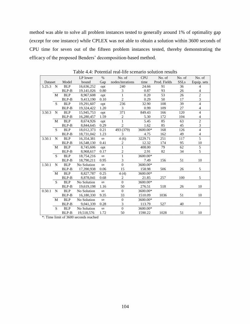
104

method was able to solve all problem instances tested to generally around 1% of optimality gap

(except for one instance) while CPLEX was not able to obtain a solution within 3600 seconds of

CPU time for seven out of the fifteen problem instances tested, thereby demonstrating the

efficacy of the proposed Benders’ decomposition-based method.

Table 4.4: Potential real-life scenario solution results

Dataset Model

LP lower

bound

%

Gap

No. of

nodes/iterations

CPU

time

No. of

Prod. Fields

No. of

SSLs

No. of

Equip. sets

5.25.3 N BLP 16,636,252 opt 240 24.66 91 36 4

BLP-B 19,141,026 0.80 3 0.87 93 26 4

M BLP 8,967,608 opt 1 0.20 53 26 2

BLP-B 9,413,190 0.10 2 0.29 50 17 3

S BLP 19,291,607 opt 236 32.90 108 39 4

BLP-B 19,324,422 1.20 3 0.99 109 27 4

3.50.3 N BLP 15,945,753 opt 371 849.43 166 120 4

BLP-B 16,280,457 1.59 2 5.30 172 104 4

M BLP 8,674,926 opt 1 5.45 85 63 2

BLP-B 8,844,645 0.29 2 1.62 85 45 3

S BLP 18,012,373 0.21 493 (379) 3600.00* 168 126 4

BLP-B 18,731,042 1.23 3 4.75 162 49 4

3.50.1 N BLP 16,354,381 4 (6) 3229.71 251 117 5

BLP-B 16,548,130 0.41 2 12.32 174 95 10

M BLP 8,745,606 opt 1 408.00 79 62 5

BLP-B 8,968,617 0.17 2 2.91 82 34 5

S BLP 18,754,216 1 3600.00*

BLP-B 18,790,211 0.95 3 7.49 156 51 10

1.50.1 N BLP No Solution 0 3600.00*

BLP-B 17,390,938 0.06 15 158.98 506 26 5

M BLP 8,827,787 0.25 4 (4) 3600.00*

BLP-B 8,878,041 0.68 2 21.85 257 100 5

S BLP No Solution 0 3600.00*

BLP-B 19,619,198 1.16 50 276.51 518 26 10

0.50.1 N BLP No Solution 0 3600.00*

BLP-B 16,180,330 9.35 33 1510.09 1036 51 10

M BLP No Solution 0 3600.00*

BLP-B 9,041,339 0.28 3 113.79 527 40 7

S BLP No Solution 0 3600.00*

BLP-B 19,518,576 1.72 50 1590.22 1028 51 10

*: Time limit of 3600 seconds reached

105

Chapter 5 Multiple Asymmetric Traveling Salesmen Problem with and without Precedence Constraints: Performance Comparison of Various Formulations

5. Hidden figure

Table 5: Hidden table

5.1. Introduction

The multiple asymmetric traveling salesmen problem arises because of the movement of

equipment sets among the SSLs in order to load trucks for highway hauling. In this chapter, we

investigate the performances of 26 formulations for the multiple asymmetric traveling salesman

problem (mATSP) from the viewpoint of their tightness and solvability using commercial

software. These formulations are either new or are generalizations of those proposed in the

literature for the ATSP, including a transformation of the mATSP to an equivalent ATSP

formulation. In particular, our results based on the latter strategy reveal that the superiority of

the original mATSP formulation over an equivalent transformed ATSP model depends upon the

type of formulation used for conducting such a transformation. We also extend our study to the

case where precedence relationships exist among the cities. We address two situations in this

context. In the first case, a sequential processing order is enforced between a pair of cities only

if they both lie on the tour of a particular salesman (designated as PCmATSP). The second case

involves a more general precedence in which a sequential processing order between certain pairs

of cities is enforced regardless of whether the designated pairs are visited by the same or by

different salesmen (designated as G-PCmATSP). Our computational experiments demonstrate

that the flow-based models afford the tightest LP relaxations. Additionally, the formulations that

model the different variants of the mATSP directly, rather than by transforming the problem to

an equivalent ATSP problem, are generally faster and more robust.

106

5.2. Problem overview

In this chapter, we study the multiple asymmetric traveling salesman problem (mATSP) in which

a given set of cities is to be visited by m salesmen such that each city is visited by exactly one

salesman and where the sum of the distances traversed by the m salesmen is minimized. Our

objective is to compare the performances of various formulations for this problem. Some of

these formulations are new, while others are those that are either directly adopted from the

literature or are modified generalizations of the ATSP. Additionally, we consider a formulation

based on the transformation of the mATSP to an equivalent ATSP. The effectiveness of these

formulations is assessed based on the CPU times required to obtain integer optimal solutions

directly by CPLEX 12.1.0, and also, based on their relative tightness, which is measured by the

closeness of their linear programming (LP) relaxation values to the optimal solution value.

We then extend our study to the case where precedence or sequential order relationships exist

among designated pairs of cities. We address two situations in this context. In the first case, a

sequential order between a pair of cities is enforced only if both cities lie on the tour of a single

salesman. We denote this problem as PCmATSP. This type of precedence is encountered in the

scheduling of steel rolling mills as reported by Appelqvist and Lehtonen [2]. The second case

involves a more general precedence in which a sequential processing order between designated

pairs of cities is enforced regardless of whether or not each city in a pair is visited by the same

salesman. We denote this problem as G-PCmATSP. Such a situation arises in the scheduling of

project networks [36, 110] on parallel resources with activities requiring sequence-dependent

setup times and where certain pairs of activities must be ordered with respect to processing times

regardless of the resource assignment.

Two recent literature reviews have been presented by Oncan et al. [108] and Bektas [7] for

ATSP and mATSP, respectively. The review by Oncan et al. covers 24 ATSP formulations, and

it presents an empirical investigation of their relative strengths. The review by Bektas provides

an overview of the formulations and solution procedures for the mATSP. It essentially discusses

four major formulations, and also presents an equivalent transformation of mATSP to ATSP. In

107

this chapter, we study a more comprehensive set of 26 formulations for the mATSP and

empirically investigate their relative performances.

The remainder of this chapter is organized as follows. In Section 5.3, we discuss the different

new and existing mATSP formulations considered herein, including the representation of the

mATSP as an equivalent ATSP model. A computational comparison of these formulations is

then presented in Section 5.4 using test cases from the TSP library as well as randomly generated

instances. Sections 5.5 and 5.6 address formulations and computational results for the

PCmATSP and G-PCmATSP, respectively, including their respective transformations to

equivalent PCATSP and G-PCATSP representations. Finally, Section 5.7 provides a summary

and concluding remarks.

5.3. Formulations for the multiple asymmetric traveling salesmen

problem

The multiple asymmetric traveling salesmen problem (mATSP) can be defined as follows: Given

a set of n cities and m traveling salesmen, determine a tour for each salesman such that, starting

from the same base city, each salesman visits at least one city and returns to the base city, where

each city is visited by exactly one salesman, and where the objective is to minimize the total

distance traveled by all the m salesmen.

The formulations for the mATSP differ by the way the subtour elimination constraints (SECs)

are modeled, where the models can be accordingly classified as follows: (i) those that are based

on the ranking of the cities, and (ii) those that are based on multi-commodity flow constructs.

(single-commodity flow-based formulations can also be included in the first class.) We discuss

model formulations based on these classes of SECs in Subsections 5.3.1 and 5.3.2, respectively.

In Subsection 5.3.3, we present formulations that rely on transformations of the mATSP to an

equivalent ATSP.

5.3.1 Formulations with SECs based on the ranking of cities

Most of the formulations in this class [18, 54, 77, 140] have extended the Miller-Tucker-Zemlin

(MTZ) [101] formulation for the single asymmetric traveling salesman problem to the m-

108

salesman case (designated as mATSP-MTZ). To present such an extension, define the decision

variables:

,0

,1ijx

if city i directly precedes city j on any tour

otherwise, ,,,...,1, jinji

iu a rank order index associated with city i, .,...,1 ni

Without loss of generality, we assume city 1 to be the base city and accordingly set and

we let where denotes the maximum number of cities from

{ } that can be visited by any salesman. Throughout the chapter, we assume that .

This yields the following basic formulation:

mATSP-MTZ: Minimize

n

i

n

ijj

ijij xc1 ,1

(5.1a)

subject to

mxn

j

j 2

1

(5.1b)

mxn

i

i 2

1

(5.1c)

n

jii

ijx,1

,1 nj ,...,2

(5.1d)

n

jij

ijx,1

,1 ni ,...,2

(5.1e)

),1(1 ijji xquu ,,...,2, nji ji

(5.1f)

,1 qui ni ,...,2

(5.1g)

},1 ,0{ijx

,,...,1, nji .ji

(5.1h)

Constraints (5.1b, c) ensure that exactly m salesmen depart from and return to the base city, and

Constraints (5.1d, e) are the classic assignment restrictions that require each city in the set

{ } to be preceded by and to precede exactly one other city. Constraints (5.1f, g) enforce

the well-known Miller-Tucker-Zemlin (MTZ) subtour elimination constraints (SECs), and (5.1h)

represents the logical restrictions on the decision variables.

109

Desrochers and Laporte [31] tightened the MTZ-based SECs for the ATSP by lifting the

corresponding constraints (5.1f, g). Kara and Bektas [77] extended these lifted MTZ SECs for

the mATSP and also imposed a minimum number ( ) of cities to be included in the tour of a

salesman. Here, we set so that each salesman needs to visit at least one city other than the

base city. The associated lifted subtour elimination constraints for the mATSP can then be stated

as follows:

,1)2( 11 qxxqu iii ni ,...,2

(5.2a)

,211 iii xxu ni ,...,2

(5.2b)

,1)2( qxqqxuu jiijji ,,...,2, nji .ji

(5.2c)

Constraints (5.2a, b) lift the bounding inequalities (5.1g), and Constraints (5.2c) lifts (5.1f).

Accordingly, the formulation mATSP-KB is given as follows:

mATSP-KB: Minimize {(5.1a): (5.1b-e, h) and (5.2a-c)}.

Gavish and Graves [55] proposed a single commodity flow model that utilizes a natural

extension of the MTZ subtour elimination constraints. This formulation (designated mATSP-

GG) requires an additional index for the -variables, where the new variable, denoted , has an

intuitive interpretation of a flow on arc (i, j) that induces a ranking similar to that in the MTZ

formulation, while additionally maintaining a path among the cities. The associated flow

constraints are given as follows:

,1,2,1

n

ijj

ji

n

ijj

ij ww ni ,...,2

(5.3a)

,0 ijij qxw ,,...,1, nji ;ji ,,...,2,01 njw j

(5.3b)

this yields the following model:

mATSP-GG: Minimize {(5.1a): (5.1b-e, h) and (5.3a, b)}.

Fox, Gavish, and Graves [49] presented a time-indexed formulation for the ATSP, where a unit

time is imposed for traveling from one city to another and is used to identify the position of a

city on a tour. In this chapter, we generalize their formulation to model the mATSP. Consider

the following variable:

110

,0

,1ijkr

if city i directly precedes city j at the kth

step of any tour

otherwise, ,,,...,1, jinji 0,..., ,k q

where the 0th

step corresponds to that from the base city for each tour. Observe that the

following relationships hold with respect to the (x, w)-variables that define mATSP-GG:

q

k

ijkij rx0

and , 0

q

k

ijkij rkw ,,...,1, nji .ji (5.4)

Accordingly, based on mATSP-GG, we derive the following formulation, where (5.5b-f)

respectively correspond to (5.1b-e) and (5.3a); (5.3b) is implied by the relationship (5.4), and

where we have restricted certain r-variable values in (5.5g) according to logical considerations:

mATSP-FGG1: Minimize

n

i

n

ijj

q

k

ijkij rc1 ,1 0

(5.5a)

subject to

mrn

j

j 2

01

(5.5b)

mrn

i

q

k

ki 2 1

1

(5.5c)

,1,1

1

0

n

iji

q

k

ijkr nj ,...,2

(5.5d)

,1,1 1

n

ijj

q

k

ijkr ni ,...,2

(5.5e)

,1,2

1

0,1 1

n

ijj

q

k

jik

n

ijj

q

k

ijk krkr ni ,...,2

(5.5f)

},1 ,0{ijkr ,,...,1, nji ,ji ;,...,0 qk with ,,...,2,01 njr jk ;,...,1 qk

;,...,2,010 njrj ,,...,2,,0 njirijk ,ji .or 0 qk (5.5g)

We can alternatively construct a disaggregated version of mATSP-FGG1 by defining the t

ijkr -

and t

jz -variables for each salesman as follows:

111

,0

,1t

ijkr if city i directly precedes city j at the k

th step of the tour by salesman t

otherwise, ,,,...,1, jinji ,,...,0 qk mt ,...,1

,0

,1t

jz if city j is visited on the tour by salesman t

otherwise, ,,...,1 nj .,...,1 mt

This yields the following formulation, where the variables of mATSP-FGG1 are related to those

for the present model via ,1

m

t

t

ijkijk rr :,,...,1, jinji

mATSP-FGG2: Minimize

n

i

n

ijj

q

k

m

t

t

ijkij rc1 ,1 0 1

(5.6a)

subject to

,11

m

t

t

iz ni ,...,2

(5.6b)

,12

01

n

j

t

jr mt ,...,1

(5.6c)

,12 1

1

n

i

q

k

t

kir mt ,...,1

(5.6d)

,,1

1

0

t

j

n

iji

q

k

t

ijk zr

,,...,2 nj mt ,...,1

(5.6e)

,,1 1

t

i

n

ijj

q

k

t

ijk zr

,,...,2 ni mt ,...,1

(5.6f)

,,2

1

0,1 1

t

i

n

ijj

q

k

t

jik

n

ijj

q

k

t

ijk zkrkr

,,...,2 ni mt ,...,1

(5.6g)

,12

1

01

2

01

n

j

t

j

n

j

t

j jrjr 1,...,1 mt

(5.6h)

,0t

iz ,,...,2 ni mt ,...,1 ;

},1 ,0{t

ijkr ,,,...,1, jinji ,,...,0 qk ,,...,1 mt with:

,,...,2,01 njr t

jk ,,...,1 qk ;,...,1 mt (5.6j)

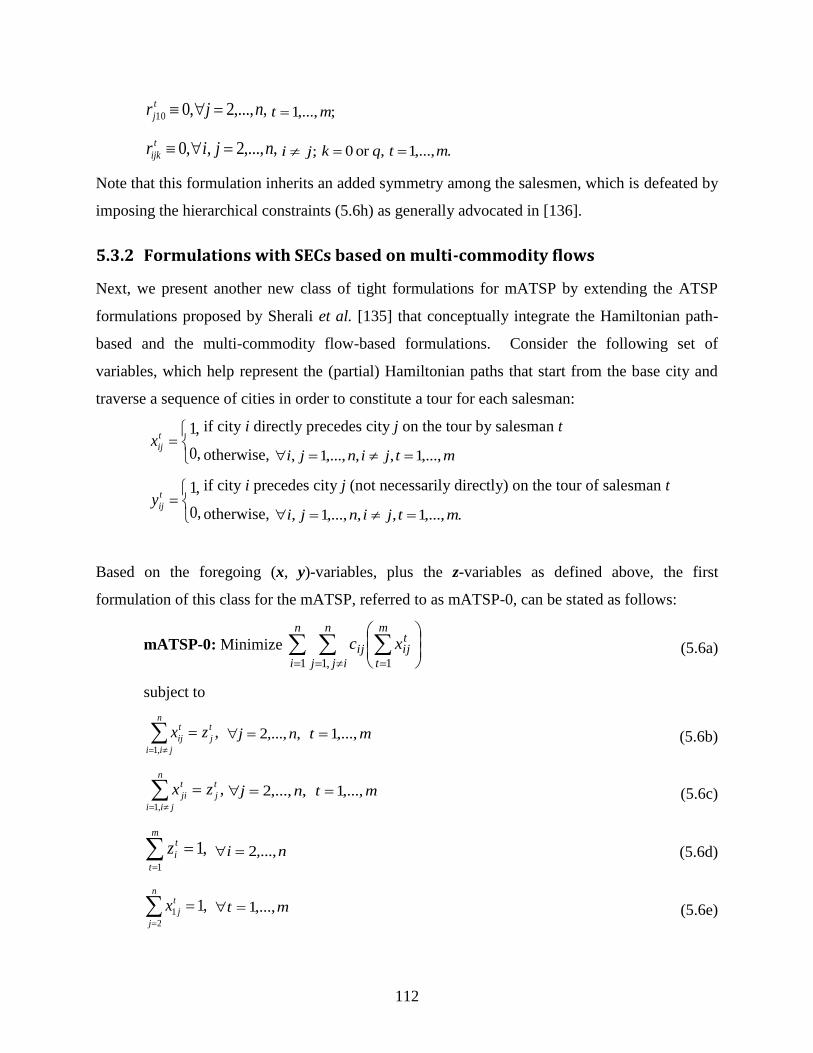
112

,,...,2,010 njr t

j ;,...,1 mt

,,...,2,,0 njir t

ijk ;ji ,or 0 qk .,...,1 mt

Note that this formulation inherits an added symmetry among the salesmen, which is defeated by

imposing the hierarchical constraints (5.6h) as generally advocated in [136].

5.3.2 Formulations with SECs based on multi-commodity flows

Next, we present another new class of tight formulations for mATSP by extending the ATSP

formulations proposed by Sherali et al. [135] that conceptually integrate the Hamiltonian path-

based and the multi-commodity flow-based formulations. Consider the following set of

variables, which help represent the (partial) Hamiltonian paths that start from the base city and

traverse a sequence of cities in order to constitute a tour for each salesman:

,0

,1t

ijx if city i directly precedes city j on the tour by salesman t

otherwise, mtjinji ,...,1,,,...,1,

,0

,1t

ijy if city i precedes city j (not necessarily directly) on the tour of salesman t

otherwise, .,...,1,,,...,1, mtjinji

Based on the foregoing (x, y)-variables, plus the z-variables as defined above, the first

formulation of this class for the mATSP, referred to as mATSP-0, can be stated as follows:

mATSP-0: Minimize

n

i

n

ijj

m

t

tijij xc

1 ,1 1 (5.6a)

subject to

,,1

t

j

n

jii

t

ij zx

,,...,2 nj mt ,...,1

(5.6b)

,,1

t

j

n

jii

t

ji zx

,,...,2 nj mt ,...,1

(5.6c)

,11

m

t

t

iz ni ,...,2

(5.6d)

,12

1

n

j

t

jx mt ,...,1

(5.6e)

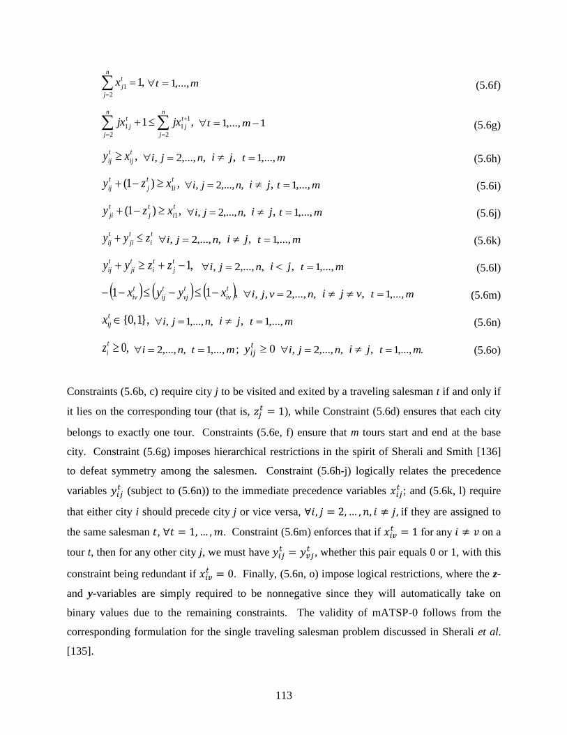
113

,12

1

n

j

t

jx mt ,...,1

(5.6f)

,12

1

1

2

1

n

j

t

j

n

j

t

j jxjx 1,...,1 mt

(5.6g)

,t

ij

t

ij xy ,,...,2, nji ,ji mt ,...,1

(5.6h)

,)1( 1

t

i

t

j

t

ij xzy ,,...,2, nji ,ji mt ,...,1

(5.6i)

,)1( 1

t

i

t

j

t

ji xzy ,,...,2, nji ,ji mt ,...,1

(5.6j)

t

i

t

ji

t

ij zyy ,,...,2, nji ,ji mt ,...,1

(5.6k)

,1 t

j

t

i

t

ji

t

ij zzyy ,,...,2, nji ,ji mt ,...,1

(5.6l)

,11 t

iv

t

vj

t

ij

t

iv xyyx ,,...,2,, nvji ,vji mt ,...,1

(5.6m)

},1 ,0{t

ijx

,,...,1, nji ,ji mt ,...,1

(5.6n)

,0t

iz ,,...,2 ni mt ,...,1 ; 0tijy ,,...,2, nji ,ji .,...,1 mt

(5.6o)

Constraints (5.6b, c) require city j to be visited and exited by a traveling salesman t if and only if

it lies on the corresponding tour (that is, ), while Constraint (5.6d) ensures that each city

belongs to exactly one tour. Constraints (5.6e, f) ensure that m tours start and end at the base

city. Constraint (5.6g) imposes hierarchical restrictions in the spirit of Sherali and Smith [136]

to defeat symmetry among the salesmen. Constraint (5.6h-j) logically relates the precedence

variables (subject to (5.6n)) to the immediate precedence variables

; and (5.6k, l) require

that either city i should precede city j or vice versa, if they are assigned to

the same salesman , . Constraint (5.6m) enforces that if for any on a

tour t, then for any other city j, we must have

, whether this pair equals 0 or 1, with this

constraint being redundant if . Finally, (5.6n, o) impose logical restrictions, where the z-

and y-variables are simply required to be nonnegative since they will automatically take on

binary values due to the remaining constraints. The validity of mATSP-0 follows from the

corresponding formulation for the single traveling salesman problem discussed in Sherali et al.

[135].

114

Furthermore, similar to the approach in Sherali et al. [135], we can tighten the formulation

mATSP-0 by applying the first-order Reformulation-Linearization Technique (RLT) process of

Sherali and Adams [129, 130]. Consider the following special RLT product constraints using

(5.6b, c) and the implied constraint 10 tvjy , njv ,...,2, , jv , mt ,...,1 (from (5.6k,

m)):

,10 t

iv

t

vj xy

,,...,1 ni ,,...,2, njv vji , mt ,...,1

(5.7a)

,,1

t

ij

t

i

n

ivv

t

iv yzx

,,...,2, nji ,ji mt ,...,1

(5.7b)

,,1

t

vj

t

v

n

vii

t

iv yzx

,,...,2, njv ,jv .,...,1 mt

(5.7c)

To linearize the product terms thus created, we define the new set of variables:

,)( t

vj

t

iv

tv

ij yxf ,,...,1 ni ,,...,2, njv ,vji .,...,1 mt

(5.8)

It is easy to show that the constraints of mATSP-0 imply the following identities:

,)( tv

ij

t

ij

t

iv fyx ,,...,2 ni ,,...,2, njv ,vji mt ,...,1

(5.9a)

,t

iv

t

iv

t

iv xyx ,,...,2, nvi ,vi mt ,...,1

(5.9b)

,0 t

vi

t

iv yx ,,...,2, nvi ,vi mt ,...,1

(5.9c)

,01 t

iv

t

i yx ,,...,2, nvi ,vi mt ,...,1

(5.9d)

,t

iv

t

iv

t

i yyz

,,...,2, nvi ,vi .,...,1 mt

(5.9e)

The identities (5.9a-e), along with (5.8), can be used in the RLT product constraints (5.7a-c) to

obtain the following respective linearized constraints (5.10a-c), where the validity of (5.10d) is

readily verified by examining the cases of t

jz equal to 0 and 1, along with the identity (5.8):

,)(0 t

iv

tv

ij xf ,,...,1 ni ,,...,2, njv ,vji mt ,...,1

(5.10a)

,)(,,2

t

ij

t

ij

n

jivv

tv

ij yxf

,,...,2, nji ,ji mt ,...,1

(5.10b)

115

,)(,,1

t

vj

n

jvii

tv

ij yf

,,...,2, njv ,jv mt ,...,1

(5.10c)

,)( 1

,2

1

t

j

t

j

n

jvv

tv

j zxf

,,...,2 nj .,...,1 mt

(5.10d)

We now augment mATSP-0 with (5.10a-d) to obtain the following tightened RLT-lifted

formulation of mATSP-0, where (5.6h) is omitted below because it is implied by (5.10a, b):

mATSP-1: Minimize {(5.6a): (5.6b-g, i-o), and (5.10a-d)}.

We shall also consider the following reduced versions of mATSP-1 obtained by deleting the

superfluous (although potentially tightening) valid inequalities (5.6i, j, m) and (5.6i, j, l, m),

respectively, where the validity of these formulations can be established using a similar proof as

presented in Sherali et al. [135] for the ATSP:

mATSP-2: Minimize {(5.6a): (5.6b-g, k, l, n, o), and (5.10a-d)}.

mATSP-2R: Minimize {(5.6a): (5.6b-g, k, n, o), and (5.10a-d)}.

Finally, we replace Constraint (5.7k) in mATSP-2R by the relaxed variable bounding restrictions

(5.11a, b) given below, in order to allow for a direct comparison with the equivalent ATSP-based

formulations presented in the next subsection.

,t

i

t

ij zy ,,...,2, nji ,ji mt ,...,1

(5.11a)

,t

j

t

ij zy ,,...,2, nji ,ji mt ,...,1

(5.11b)

mATSP-2R-: Minimize {(5.6a): (5.6b-g, n, o), (5.10a-d), and (11a, b)}.

On the other hand, we can further lift mATSP-2 by adding back the valid inequalities (5.6i, j)

along with the following additional restrictions [120] on the y-variables:

,2 t

ki

t

jk

t

ji

t

ij yyxy ,,...,1,, nkji ,kji .,...,1 mt

(5.12)

This yields the formulation mATSP-6 stated below.

mATSP-6: Minimize {(5.6a): (5.6b-g, i-l, n, o), (5.10a-d), and (5.12)}.

116

Laporte and Norbert [86] extended the ATSP formulation of Dantzig-Fulkerson-Johnson (DFJ)

[25] to the m-salesman case, and adopted an LP-based relaxation approach that imposes subtour

elimination and integrality restrictions when needed. Wong [150] established the equivalence of

a polynomial length maximum flow-based formulation for ATSP to the exponentially-sized

formulation based on the DFJ subtour elimination constraints. This equivalence holds for the m-

salesman versions of these respective formulations as well. Below, we provide a new model

(mATSP-FL1) for mATSP that is a generalization of the model proposed for ATSP in [150].

Due to the presence of m salesmen, we also include certain symmetry breaking constraints.

Consider the following set of decision variables, in addition to the (x, z)-variables defined above:

,0

,1

)( tv

ijp

if flow occurs on arc (i, j) for the vth

commodity sent from the base city 1 to

city v via the tour of salesman t

otherwise, .,...,1,,...,2,,,...,1, mtnvjinji

The flow-based formulation for the mATSP, referred to as mATSP-FL1, can be stated as

follows:

mATSP-FL1: Minimize

n

i

n

ijj

m

t

t

ijij xc1 ,1 1

(5.13a)

subject to

,,1

t

j

n

jii

t

ij zx

,,...,2 nj mt ,...,1

(5.13b)

,,1

t

j

n

jii

t

ji zx

,,...,2 nj mt ,...,1

(5.13c)

,11

m

t

t

iz ni ,...,2

(5.13d)

,12

1

n

j

t

jx mt ,...,1

(5.13e)

,12

1

n

j

t

jx mt ,...,1

(5.13f)

,12

1

1

2

1

n

j

t

j

n

j

t

j jxjx 1,...,1 mt

(5.13g)

117

,)( t

ij

tv

ij xp ,,...,1, nji ,ji ,,...,2 nv mt ,...,1

(5.13h)

,)(2

1

t

v

n

j

tv

j zp

,,...,2 nv mt ,...,1

(5.13i)

,0)()(,1,2

n

ijj

tv

ji

n

ijj

tv

ij pp ,,...,2, nvi ,vi mt ,...,1

(5.13j)

,)(,1

t

v

n

vjj

tv

jv zp

,,...,2 nv mt ,...,1

(5.13k)

},1 ,0{t

ijx ,,...,1, nji ,ji mt ,...,1

(5.13l)

,0t

iz ,,...,2 ni mt ,...,1

(5.13m)

,0)( tv

ijp

,,...,1, nji ,ji ,n,...,v 2 ,,...,1 mt

with ,0)( 1 tv

jp ,,...,2 nj ,,...,2 nv ,jv ;,...,1 mt and

,0)( tv

vjp ,,...,1 nj ,,...,2 nv ,jv .,...,1 mt

(5.13n)

Constraints (5.13b-g) are identical to Constraints (5.6b-g) in mATSP-0. Constraints (5.13h-k)

are used to model multi-commodity flows, each related to . In particular, for each

salesman, Constraint (5.13h) allows flow to occur from city i to city j only if , and

Constraints (5.13i-k) constitute flow balance restrictions. Constraints (5.13l-n) impose logical

restrictions on the decision variables, where again, the integrality of the (z, p)-variables follows

from the remaining model constraints.

The above interpretation of the p-variables supports the following additional valid restrictions:

,)( 11

t

v

tv

v xp ,,...,2 nv mt ,...,1

(5.14a)

,)( t

jv

tv

jv xp ,,...,2, nvj ,vj mt ,...,1 .

(5.14b)

By substituting (5.14a, b) in mATSP-FL1, we can show that (5.13k) can be omitted since using

(5.13m, 5.14a, b), this reduces to (5.13b) written for . Furthermore, (5.13i, j) can be

rewritten in the following strengthened form given by (5.15a, b), respectively:

,)( 11

,2

t

v

t

v

tv

j

n

vjj

zxp

,,...,2 nv mt ,...,1

(5.15a)

118

,0)()(,,1,,2

tv

ji

n

vijj

t

iv

tv

ij

n

vijj

pxp ,,...,2, nvi ,vi .,...,1 mt

(5.15b)

Consequently, we propose the following tightened reformulated version of mATSP-FL1:

mATSP-FL2: Minimize {(5.13a): (5.13b-h, l-n), and (5.15a, b)}.

5.3.3 Transformation of mATSP to an equivalent ATSP

Another approach to solve the mATSP is to transform it into an equivalent ATSP. Svestka and

Huckfeldt [140] and Bellmore and Hong [8] have proposed an augmented distance matrix by

including additional rows and columns, where each new row and column is

respectively a duplicate of the base city row and column of the original matrix, and where

infinite distances are assigned to all new elements. The alternative transformations of the

mATSP to an equivalent ATSP are similar with differences being with respect to: (i) the set of

newly created arcs that are utilized in the symmetric TSP problem [72], and (ii) the cost structure

used, i.e., whether or not a cost is assigned for utilizing the salesman [8, 61]. Figure 5.1 depicts

an equivalent ATSP solution for the mATSP problem with , where the tours of the three

salesmen are { } { } and { }. Note that the base city 1 is duplicated m

times as to differentiate among the m tours by identifying the beginning and end

of each tour.

A major difficulty encountered while solving the equivalent ATSP representation is that an

optimal solution for the original mATSP corresponds to m! optimal solutions of the ATSP due to

the inherent symmetry among salesmen [72], which is more so than in the mATSP-FL1 model

above because any given set of tours for the m salesmen can be further permuted arbitrarily and

concatenated into a single tour solution for the ATSP-based representation. To mitigate this

symmetry, which can impair the solution of the transformed model, we add hierarchical

constraints (see [136]) when more than two salesmen are involved, as given by (5.16d, f) below.

119

Figure 5.1: An ATSP solution for the mATSP problem with

We consider several ATSP formulations to effectively model this transformation. These include

the classic ATSP-MTZ formulation [101], four ATSP formulations as proposed by Sherali et al.

[135], namely ATSP-2, ATSP-2R, ATSP-2R-, and ATSP-6, which are considered due to their

superior performance in generating tight LP relaxations as reported in their chapter and further

analyzed by Oncan et al. [108], and also, the flow-based models presented in [135]. These

models are presented below, where 2' nmq :

ATSP-MTZ: Minimize

n

i

n

ijj

ijij xc1 11 ,1

(5.16a)

subject to

n

jii

ijx,11

,1 nj m ,...,2,1,...,11

(5.16b)

n

jij

ijx,11

,1 ni m ,...,2,1,...,11

(5.16c)

,12

1

2

1 1

n

j

j

n

j

j ttjxjx

1,...,1 mt

(5.16d)

),1('1 ijji xquu ,n,...,,,...,j,i m 2112 ji

(5.16e)

,uutt

211 1

;1,...,1 mt and 0

11 u

(5.16 f)

11

2

12

13

3

4 5

7

6

120

,'1 qui ni m ,...,2,1,...,12

(5.16g)

},1 ,0{ijx

,,...,2,1,...,1, 1 nji m ;ji with ,0'11

ttx ,,...,1', mtt '.tt

(5.16h)

In a similar manner as before (see [31, 77]), Constraints (5.16e, g) can be lifted as follows:

,1')2'(11 11 qxxqu iii ,,...,2,1,...,12 ni m

(5.17a)

,2)2'(11 11 iii xqxu ,,...,2,1,...,12 ni m

(5.17b)

,1')2'(' qxqxquu jiijji ,,...,2,1,...,1, 2 nji m .ji

(5.17c)

Consequently, the formulation ATSP-KB is given as follows:

ATSP-KB: Minimize {(5.16a): (5.16b-d, f, h) and (5.17a-c)}.

We can modify the formulation by Gavish and Graves [55] for use in the transformed problem as

well by adapting (5.3a, b) and (5.16f) as follows:

,1,1,1 21

n

ijj

ji

n

ijj

ij ww ni m ,...,2,1,...,12

(5.18a)

,'0 ijij xqw ,,...,2,1,...,1, 1 nji m ;ji ,011 jw nj m ,...,2,1,...,12 (5.18b)

,211 1

1

1,1 1,1

11

n

jj

n

jj

jj

t t

ttww .1,...,1 mt (5.18c)

This yields the following revised valid formulation:

ATSP-GG: Minimize {(5.16a): (5.16b-d, h) and (5.18a-c)}.

Similarly, the formulation of Fox et al. [49] can be transformed into an equivalent ATSP

formulation as follows, where we now also add a constraint (5.19d) for each step in the tour;

Constraints (5.19f) and (5.19g) respectively imitate the symmetry defining Constraints (5.16d)

and (5.16f), and where (5.19h) logically restricts certain stated r-variables to zero:

ATSP-FGG1: Minimize

n

i

n

ijj

q

k

ijkij rc1 11 ,1

'

0

(5.19a)

subject to

,1,1

'

01

n

ijj

q

k

ijkr ni m ,...,2,1,...,11

(5.19b)

121

,1,1

'

01

n

iji

q

k

ijkr nj m ,...,2,1,...,11

(5.19c)

,11 11 ,1

n

i

n

ijj

ijkr ',...,0 qk

(5.19d)

,1,1

'

0,1

'

1 11

n

ijj

q

k

jik

n

ijj

q

k

ijk krkr ni m ,...,2,1,...,12

(5.19e)

,12

1'

1

1

2

1'

0

1 1

n

j

q

k

jk

n

j

q

k

jk ttjrjr 1,...,1 mt

(5.19f)

,22

1'

0

1

2

1'

1

1 1

n

j

q

k

jk

n

j

q

k

jk ttkrkr 1,...,1 mt

(5.19g)

},1 ,0{ijkr ,,...,2,1,...,1, 1 nji m ,ji ;',...,0 qk with

,,...,2,1,...,1,0 211njr mjk ;',...,1 qk

,,...,2,1,...,1,0 211njr mkj ;1',...,0 qk

,,...,2,1,...,1,,0 2 njir mijk ;ji

;'or 0 qk ,1,...,1,,0 2 mijk jir ;ji '.,...,0 qk (5.19h)

As modeled in [49], a relaxation of ATSP-FGG1 can be considered by removing Constraint

(5.19d) from the formulation, thus yielding the following formulation:

ATSP-FGG2: Minimize {(5.19a): (5.19b, c, e-h)}.

Oncan et al. [108] have shown that the ATSP models derived by Sherali et al. [135] are among

the tightest known polynomial length formulations. Next, we adapt these formulations to

transform mATSP to an equivalent ATSP. Consider the following variables:

1,

0,ijy

if city i precedes city j (not necessarily directly)

otherwise, ,,...,2,1,...,1, 2 nji m ji

,0

,1j

ivf if flow occurs on arc (i, j) for the v

th commodity sent from the base city 1 to city v

otherwise, ,,...,2,1,...,11 ni m ,,...,2,1,...,1, 2 nvj m ,vi .ji

Note that these variables are identical to those defined earlier for mATSP-0, except that they are

not associated with a particular tour t. This yields the following formulation:

122

ATSP-0: Minimize

n

i

n

ijj

ijij xc1 11 ,1

(5.20a)

subject to

n

jii

ijx,11

,1 nj m ,...,2,1,...,11

(5.20b)

n

jij

ijx,11

,1 ni m ,...,2,1,...,11

(5.20c)

,12

1

2

1 1

n

j

j

n

j

j ttjxjx

1,...,1 mt

(5.20d)

,111 lk

y mlk 2

(5.20e)

,ijij xy ,,...,2,1,...,1, 2 nji m ji

(5.20f)

,11 iij xy ,,...,2 ni ,,...,2,1,...,12 nj m ji

(5.20g)

,11iji xy ,,...,2 ni ,,...,2,1,...,12 nj m ji

(5.20h)

,1 jiij yy ,,...,2,1,...,1, 2 nji m ji

(5.20i)

,11 ivvjijiv xyyx ,,...,2,1,...,1,, 2 nvji m vji

(5.20j)

},1 ,0{ijx

,,...,2,1,...,1, 1 nji m ;ji with ,0

'11 tt

x ,,...,1', mtt 'tt

(5.20k)

0ijy ,,...,2,1,...,1, 2 nji m .ji

(5.20l)

ATSP-0 can be tightened in a similar fashion to mATSP-1 through the RLT process as in Sherali

et al. [135] to yield the following constraints:

,0 iv

v

ij xf ,,...,2,1,...,11 ni m ,,...,2,1,...,1, 2 nvj m ,vi ji

(5.21a)

,,,12

ijij

n

jivv

v

ij yxf

,,...,2,1,...,1, 2 nji m ji

(5.21b)

,1

2

1

},{,1

vjv

n

jvii

v

ij yxf

,,...,2,1,...,1, 2 nvj m .jv

(5.21c)

This leads to the following tightened RLT-lifted reformulation, where we have omitted (5.20f),

noting that this in now implied by (5.21b):

123

ATSP-1: Minimize {(5.20a): (5.20b-e, g-l), and (5.21a-c)}.

In a manner consistent with the mATSP formulations, we next consider the following reduced

version of ATSP-1 by deleting the superfluous (though tightening) valid inequalities (5.20g, h, j):

ATSP-2: Minimize {(5.20a): (5.20b-e, i, k, l), and (5.21a-c)}.

By relaxing Constraints (5.20i) to

,1 jiij yy ,,...,2,1,...,1, 2 nji m ,ji

(5.22)

we obtain another valid formulation ATSP-2R stated below, which is a relaxation of ATSP-2:

ATSP-2R: Minimize {(5.20a): (5.20b-e, k, l), (5.21a-c), and (5.22)}.

Furthermore, as established in [135], we can derive the following alternative valid formulation

that is a further relaxation of ATSP-2, denoted by ATSP-2R-, in which the Constraints (5.20i) are

entirely deleted from the model:

ATSP-2R-: Minimize {(5.20a): (5.20b-e, k, l), and (5.21a-c)}.

Again, we further modify ATSP-1 be replacing (5.20j) with the following restriction on the y-

variables (see [120]):

,2 kijkjiij yyxy ,,...,2,1,...,1,, 2 nkji m .kji

(5.23)

This yields the formulation ATSP-6 stated below:

ATSP-6: Minimize {(5.20a): (5.20b-e, g-i, k, l), (5.21a-c), and (5.23)}.

We can also use the flow-based formulations for ATSP presented in [135] as discussed in

Subsection 5.5.2 above, predicated on the following decision variables:

,0

,1v

ijp

if flow occurs on arc (i, j) for the vth

commodity sent from the base city to city v

otherwise, ,,...,2,1,...,11 ni m ,,...,2,1,...,1, 2 nvj m ,vi ji

The first such flow-based formulation is given as follows:

ATSP-FL1: Minimize

n

i

n

ijj

ijij xc1 11 ,1

(5.24a)

124

subject to

n

jii

ijx,11

,1 nj m ,...,2,1,...,11

(5.24b)

n

jij

ijx,11

,1 ni m ,...,2,1,...,11

(5.24c)

,12

1

2

1 1

n

j

j

n

j

j ttjxjx

1,...,1 mt

(5.24d)

,ij

v

ij xp ,,...,2,1,...,11 ni m ,,...,2,1,...,1, 2 nvj m ,vi ji

(5.24e)

,12

11

n

j

v

jp nv m ,...,2,1,...,12

(5.24f)

,0},{,1,1 12

n

vijj

v

ji

n

ijj

v

ij pp ,,...,2,1,...,1, 2 nvi m vi

(5.24g)

,1,11

n

vjj

v

jvp nv m ,...,2,1,...,12

(5.24h)

,12

1

11

n

j

jt

tp 1,...,1 mt

(5.24i)

},1 ,0{ijx

,,...,2,1,...,1, 1 nji m ;ji with ,0'11

ttx ,,...,1', mtt 'tt

(5.24j)

,0v

ijp ,,...,2,1,...,11 ni m ,,...,2,1,...,1, 2 nvj m ,vi ;ji with

,0'11 v

ttp ,,...,1', mtt ,'tt .,...,2,1,...,12 nv m (5.24k)

ATSP-FL1 can be tightened by replacing Constraints (5.24f-h) with the following, based on

equating ,iv

v

iv xp ,,...,2,1,...,11 ni m ,,...,2,1,...,12 nv m iv (see [135]):

,1)(11 11

,2

v

v

j

n

vjj

xp nv m ,...,2,1,...,12

(5.25a)

,0},{,1},{,1 12

n

vijj

v

jiiv

n

vijj

v

ij pxp ,,...,2,1,...,1, 2 nvi m ,vi

(5.25b)

this yields the lifted model stated below:

ATSP-FL2: Minimize {(5.24a): (5.24b-e, j, k), and (5.25a, b)}.

125

5.4. Computational comparison of various mATSP formulations

For experimental purposes, we considered three standard test problems from the TSPLIB [1],

namely br17, ftv33, and ftv35, as well as a set of randomly generated problems involving 10, 12,

20, and 30 cities. The random problems were generated using Euclidean distances between

cities. For each test case, the number of salesmen (m) was varied from 2 to 4. The computations

were performed using CPLEX 12.1.0 with OPL 6.3 on an Intel Xeon E5335 2.00 GHz computer

having 3 GB of RAM and running Windows XP SP2.

The results for the TSP Library dataset are displayed in Tables 5.1 and 5.2 for the mATSP and

their equivalent ATSP formulations, respectively. Similar results were obtained for the

randomly generated data, which are not included here for the sake of brevity, but are available

online as supplementary data at http://www.sciencedirect.com. Tables 5.1 and 5.2 report the

lower bound value obtained by solving the LP relaxation, the percentage gap between the

LP-based lower bound and the optimal integer solution value (calculated as (1 /

), the respective CPU times required to derive the LP relaxation solution (CPU-LP) and

the integer optimal solution (CPU-MIP), the number of nodes generated by the branch-and-

bound algorithm, and the value of the incumbent solution whenever the algorithm terminated

prematurely. Additionally, the average, minimum, and maximum statistics over all the datasets

are reported at the bottom of the tables. For problems not solved to optimality within a pre-

specified time limit of 3600 seconds, we report the incumbent solution value at termination, if

available. The best performance value for each measure as obtained for any test problem is

highlighted in the tables by shading it. Additionally, for each test problem, the best overall

performance of each measure over all the models in both Tables 5.1 and 5.2 is highlighted in

bold-face.

Note that ATSP-6 yielded the tightest LP relaxation bounds from among all the mATSP and

equivalent ATSP models tested. For direct solution by CPLEX, the models mATSP-KB and

mATSP-MTZ generally required the smallest CPU times to obtain integer optimal solutions.

Observe that these models also enumerated the largest number of nodes because of their

relatively weak LP relaxation bounds.

126

Table 5.1: Comparison of the mATSP models Test

Problem Measure

mATSP

-MTZ

mATSP

-KB

mATSP

-GG

mATSP

-FGG1

mATSP

-FGG2

mATSP

-0

mATSP

-1

mATSP

-2

mATSP

-2R

mATSP

-2R-

mATSP

-6

mATSP

-FL1

mATSP

-FL2

br17 ZLP 8.13 22.00 12.93 14.75 14.75 25.40 39.00 39.00 39.00 39.00 39.00 39.00 39.00 m=2 %Gap 79.15 43.59 66.84 62.18 62.18 40.00 0.00 0.00 0.00 0.00 0.00 0.00 0.00 Sol’n CPU-LP 0.03 0.05 0.05 0.12 0.08 0.09 21.30 3.66 1.49 1.34 9.26 1.10 1.65 39 CPU-MIP 0.40 0.39 0.33 5.55 283.86 3600.00 208.07 17.54 10.18 2.37 12.87 3.54 5.76 # of Nodes 926 879 0 3779 21038 13405 0 0 0 0 0 0 0

Incumbent 39

br17 ZLP 14.29 28.00 19.43 21.18 21.18 29.30 42.00 42.00 42.00 42.00 42.00 42.00 42.00 m=3 %Gap 65.99 33.33 53.74 49.57 49.57 30.24 0.00 0.00 0.00 0.00 0.00 0.00 0.00 Sol’n CPU-LP 0.03 0.07 0.05 0.06 0.11 0.12 20.28 10.11 10.73 5.72 14.60 2.69 2.62 42 CPU-MIP 0.22 0.09 0.09 2.06 3600.00 3600.00 582.77 20.73 5.79 10.73 403.18 6.65 7.29 # of Nodes 403 107 0 476 303834 2460 0 0 0 0 0 0 0

Incumbent 42 42

br17 zLP 20.46 34.00 26.00 27.70 27.70 35.20 47.00 47.00 47.00 47.00 47.00 47.00 47.00 m=4 %Gap 56.47 27.66 44.68 41.07 41.07 25.11 0.00 0.00 0.00 0.00 0.00 0.00 0.00 Sol’n CPU-LP 0.03 0.05 0.05 0.09 0.12 0.19 30.35 8.57 6.31 4.67 15.62 4.47 3.09 47 CPU-MIP 0.14 0.10 0.28 4.03 2127.79 3600.00 956.31 13.58 25.42 22.79 962.90 13.75 4.42 # of Nodes 296 68 43 1299 88643 1004 0 0 0 0 0 0 0

Incumbent 47

ftv33 ZLP 1211.10 1234.50 1215.90 1216.58 1216.58 1232.00 1286.00 1302.00 1302.00 1302.00 1302.00 1302.00 1302.00 m=2 %Gap 6.98 5.18 6.61 6.56 6.56 5.38 1.23 0.00 0.00 0.00 0.00 0.00 0.00 Sol’n CPU-LP 0.04 0.05 0.07 0.15 0.37 0.64 3600.00 59.54 24.60 22.33 2921.48 63.57 60.30 1302 CPU-MIP 0.42 0.51 1.00 3600.00 3600.00 3600.00 3600.00 120.77 43.30 40.15 3600.00 37.55 37.94 # of Nodes 37 98 0 40549 8173 417 0 0 0 0 0 0 0 Incumbent * * 132 *

*

ftv33 ZLP 1238.00 1260.50 1242.40 1243.01 1243.01 1258.00 1262.00 1328.00 1328.00 1328.00 1305.00 1328.00 1328.00 m=3 %Gap 6.78 5.08 6.45 6.40 6.40 5.27 4.97 0.00 0.00 0.00 1.73 0.00 0.00 Sol’n CPU-LP 0.04 0.05 0.07 0.12 0.62 2.22 3600.00 679.62 656.57 932.58 3600.00 293.94 237.96 1328 CPU-MIP 0.44 0.58 0.86 3600.00 3600.00 3600.00 3600.00 163.69 219.97 138.11 3600.00 178.53 180.76 # of Nodes 81 246 123 87876 9756 303 0 0 0 0 0 0 0 Incumbent 1535 * 1386 *

*

ftv33 ZLP 1266.10 1302.90 1270.60 1271.32 1271.32 1300.00 1300.00 1367.00 1367.00 1367.00 1285.33 1367.00 1367.00 m=4 %Gap 7.38 4.69 7.05 7.00 7.00 4.90 4.90 0.00 0.00 0.00 5.97 0.00 0.00 Sol’n CPU-LP 0.03 0.06 0.12 0.16 1.11 2.66 3600.00 1381.21 2049.19 2769.68 3600.00 877.55 532.85 1367 CPU-MIP 0.53 0.67 1.27 3600.00 3600.00 3600.00 3600.00 1408.59 722.99 960.75 3600.00 459.73 253.47 # of Nodes 176 137 34 59589 3029 169 0 0 0 0 0 0 0 Incumbent * * 1497 *

*

ftv35 ZLP 1395.40 1425.70 1401.40 1402.30 1402.30 1425.00 1465.00 1466.50 1466.50 1466.50 1466.00 1466.50 1466.50 m=2 %Gap 6.28 4.24 5.88 5.82 5.82 4.30 1.61 1.51 1.51 1.50 1.54 1.50 1.50 Sol’n CPU-LP 0.04 0.05 0.10 0.23 0.35 1.09 3600.00 234.69 93.80 122.24 3600.00 48.95 50.46 1489 CPU-MIP 1.42 1.91 2.30 3600.00 3600.00 3600.00 3600.00 3600.00 2438.66 1998.61 3600.00 144.96 102.37 # of Nodes 707 703 59 29715 10965 864 0 0 107 115 0 91 74 Incumbent * 1848 1489 * 1518

*

ftv35 ZLP 1422.00 1467.40 1428.20 1428.93 1428.93 1467.00 1467.00 1495.50 1495.50 1495.50 1467.33 1495.50 1495.50 m=3 %Gap 5.89 2.89 5.48 5.43 5.43 2.91 2.91 1.03 1.03 1.03 2.89 1.03 1.03 Sol’n CPU-LP 0.03 0.05 0.09 0.27 0.84 2.59 3600.00 1525.37 2575.52 1355.06 3600.00 379.15 351.98 1511 CPU-MIP 0.90 0.77 2.05 3600.00 3600.00 3600.00 3600.00 3600.00 2476.40 3600.00 3600.00 654.07 3600.00 # of Nodes 620 523 23 43726 2546 82 0 0 72 6 0 119 76 Incumbent 1918 * 1564 * *

1514 *

1511

ftv35 ZLP 1464.10 1511.20 1469.00 1469.64 1469.64 1511.00 1511.00 1539.50 1539.00 1539.00 1473.00 1539.50 1539.50 m=4 %Gap 5.60 2.57 5.29 5.25 5.25 2.58 2.58 0.74 0.77 0.77 5.03 0.74 0.74 Sol’n CPU-LP 0.04 0.05 0.10 0.12 2.99 3.76 3600.00 3600.00 3600.00 3600.00 3600.00 1409.50 1041.50 1551 CPU-MIP 0.76 0.79 1.09 3600.00 3600.00 3600.00 3600.00 3600.00 3600.00 3600.00 3600.00 1991.00 1625.20

# of Nodes 314 590 203 59129 639 63 0 0 0 0 0 59 84

Incumbent 1624 * 1612 * * * * * Average ZLP 383.39 395.29 385.64 386.11 386.11 395.04 401.62 411.59 411.56 411.73 402.15 411.59 411.59

%Gap 30.30 13.02 24.71 22.99 22.99 1.17 1952.69 837.49 687.50 0.23 11.65 0.28 0.28

CPU-LP 0.03 0.05 0.07 0.10 0.42 0.94 1620.94 520.12 527.62 517.54 1531.21 173.42 128.70

CPU-MIP 0.67 0.62 0.72 1479.57 1823.77 1566.65 1717.38 792.89 652.16 684.18 1665.44 250.36 341.89 # of Nodes 458 451 31 19713 24440 956 0 0 10 6 0 14 12 Min ZLP 0.49 0.78 0.58 0.63 0.63 0.78 0.03 0.86 0.86 0.86 0.02 0.86 0.86

%Gap 5.60 0.00 5.29 5.25 5.25 2.58 0.00 0.00 0.00 0.00 0.00 0.00 0.00

CPU-LP 0.03 0.05 0.04 0.04 0.04 0.05 0.13 0.06 0.05 0.06 0.12 0.05 0.04

CPU-MIP 0.07 0.04 0.09 2.06 0.37 0.07 0.13 0.05 0.05 0.04 0.13 0.03 0.04 # of Nodes 0 0 0 45 76 0 0 0 0 0 0 0 0 Max ZLP 1464.10 1511.20 1469.00 1469.64 1469.64 1511.00 1511.00 1539.50 1539.00 1539.00 1473.00 1539.50 1539.50

%Gap 79.15 43.59 66.84 62.18 62.18 67.60 5.09 1.51 1.51 1.50 97.47 1.50 1.50

CPU-LP 0.04 0.08 0.12 0.27 2.99 3.76 3600.00 3600.00 3600.00 3600.00 3600.00 1409.50 1041.50

CPU-MIP 3.06 2.19 2.30 3610.71 3600.00 3600.00 3600.00 3600.00 3600.00 3600.00 3600.00 1991.00 3600.00 # of Nodes 3823 4428 203 87876 303834 13405 0 0 107 115 0 119 84

* No feasible solution found within 3,600 seconds of CPU time

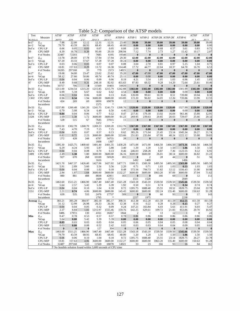
127

Table 5.2: Comparison of the ATSP models Test

Problem Measure

ATSP

-MTZ

ATSP

-KB

ATSP

-GG

ATSP

-FGG1

ATSP

-FGG2 ATSP-0 ATSP-1 ATSP-2 ATSP-2R ATSP-2R- ATSP-6

ATSP

-FL1

ATSP

-FL2 br17 ZLP 7.88 22.00 12.12 12.31 12.31 23.40 39.00 39.00 39.00 39.00 39.00 39.00 39.00 m=2 %Gap 79.79 43.59 68.93 68.45 68.45 40.00 0.00 0.00 0.00 0.00 0.00 0.00 0.00

Sol’n CPU-LP 0.06 0.05 0.03 0.07 0.05 0.08 2.09 1.89 0.68 0.57 3.61 0.83 0.71

39 CPU-MIP 8.39 16.78 0.39 95.00 29.10 298.94 7.12 7.74 2.73 1.27 15.42 10.17 2.07

# of Nodes 32487 72203 7 7685 6195 10540 0 0 0 0 0 0 0

br17 ZLP 13.78 28.00 17.78 17.94 17.94 29.30 42.00 42.00 42.00 42.00 42.00 42.00 42.00 m=3 %Gap 67.20 33.33 57.67 57.28 57.28 30.24 0.00 0.00 0.00 0.00 0.00 0.00 0.00

Sol’n CPU-LP 0.03 0.06 0.03 0.07 0.07 0.08 3.04 2.70 0.81 0.97 5.15 1.04 0.75

42 CPU-MIP 10.81 157.63 0.29 13.72 16.38 514.48 17.72 44.77 22.04 18.37 64.70 16.76 6.53

# of Nodes 16285 297168 33 779 2573 14921 0 0 0 0 0 0 0

br17 ZLP 19.68 34.00 23.47 23.62 23.62 35.20 47.00 47.00 47.00 47.00 47.00 47.00 47.00

m=4 %Gap 58.12 27.66 50.06 49.74 49.74 25.11 0.00 0.00 0.00 0.00 0.00 0.00 0.00 Sol’n CPU-LP 0.04 0.04 0.06 0.09 0.06 0.19 4.21 3.54 1.05 1.03 6.96 1.45 1.03

47 CPU-MIP 8.49 0.68 0.31 248.18 82.92 455.63 87.83 69.32 9.28 14.20 72.64 25.61 10.46

# of Nodes 10757 706 0 11569 10403 10920 0 0 0 0 0 0 0

ftv33 ZLP 1211.00 1234.54 1215.20 1215.85 1215.79 1242.88 1302.00 1302.00 1302.00 1302.00 1301.99 1302.00 1302.00

m=2 %Gap 6.99 5.18 6.67 6.62 6.62 4.54 0.00 0.00 0.00 0.00 0.00 0.00 0.00

Sol’n CPU-LP 0.06 0.04 0.06 0.69 0.13 0.45 120.09 99.61 10.39 8.51 720.80 10.04 8.30 1302 CPU-MIP 0.96 0.34 1.94 3600.00 3600.00 103.85 115.20 96.82 14.05 12.26 720.86 13.99 12.55

# of Nodes 434 269 69 6850 69078 12 0 0 0 0 0 0 0

Incumbent 1575 *

ftv33 ZLP 1237.80 1260.48 1241.20 1241.75 1241.73 1268.76 1328.00 1328.00 1328.00 1328.00 1327.99 1328.00 1328.00

m=3 %Gap 6.79 5.08 6.54 6.49 6.50 4.46 0.00 0.00 0.00 0.00 0.00 0.00 0.00

Sol’n CPU-LP 0.04 0.04 0.06 0.77 0.12 0.47 217.41 179.18 13.92 16.04 961.46 15.89 12.91 1328 CPU-MIP 1.69 1.38 1.72 3600.00 3600.00 91.23 269.95 239.63 20.85 20.03 729.07 25.66 20.32

# of Nodes 528 515 67 7645 37015 11 0 0 0 0 0 0 0

Incumbent 1472 *

ftv33 ZLP 1265.50 1302.78 1268.70 1269.23 1269.20 1312.76 1367.00 1367.00 1367.00 1367.00 1367.00 1367.00 1367.00

m=4 %Gap 7.43 4.70 7.19 7.15 7.15 3.97 0.00 0.00 0.00 0.00 0.00 0.00 0.00

Sol’n CPU-LP 0.04 0.05 0.07 0.57 0.13 0.62 385.26 171.04 21.45 23.14 1045.34 26.27 21.74 1367 CPU-MIP 0.82 0.72 2.23 3600.00 3600.00 523.66 251.83 235.84 67.99 48.24 1222.12 55.88 59.83

# of Nodes 272 428 248 4797 34755 28 0 0 0 0 0 0 0

Incumbent 1608 1367

ftv35 ZLP 1395.30 1425.75 1400.60 1401.44 1401.35 1438.29 1471.08 1471.00 1466.50 1466.50 1473.16 1466.50 1466.50

m=2 %Gap 6.29 4.24 5.93 5.87 5.88 3.40 1.20 1.20 1.50 1.50 1.06 1.50 1.50

Sol’n CPU-LP 0.04 0.04 0.08 0.70 0.13 0.46 246.03 258.28 8.87 7.36 1123.55 8.12 6.91 1489 CPU-MIP 2.49 1.38 1.80 3600.00 3600.00 36.16 3600.00 3600.00 26.01 38.14 3600.00 36.82 31.22

# of Nodes 927 670 268 10100 50528 181 0 2 28 44 0 51 56

Incumbent 1616 * 1492 1489

1496

ftv35 ZLP 1421.70 1467.37 1426.40 1427.06 1427.02 1477.71 1500.33 1500.30 1495.50 1495.50 1503.00 1495.50 1495.50

m=3 %Gap 5.91 2.89 5.60 5.56 5.56 2.20 0.71 0.71 1.03 1.03 0.53 1.03 1.03

Sol’n CPU-LP 0.04 0.04 0.08 1.02 0.18 0.48 572.56 794.73 11.82 12.12 1556.43 11.00 10.98 1511 CPU-MIP 2.94 1.87 1.64 3600.00 3600.00 1132.27 3600.00 3600.00 1863.20 97.09 3600.00 37.04 71.62

# of Nodes 980 881 488 8838 42811 183 0 0 166 69 0 12 112

Incumbent 1609 1772 1511 1528

2049

ftv35 ZLP 1463.60 1511.21 1466.90 1467.40 1467.40 1521.28 1543.18 1543.10 1539.50 1539.50 1545.66 1539.50 1539.50

m=4 %Gap 5.64 2.57 5.42 5.39 5.39 1.92 0.50 0.51 0.74 0.74 0.34 0.74 0.74

Sol’n CPU-LP 0.04 0.04 0.10 1.04 0.18 0.72 1205.75 1688.40 25.55 18.52 1828.75 23.04 22.78 1551 CPU-MIP 2.21 0.74 4.06 3600.00 3600.00 145.45 3600.00 3600.00 192.24 135.40 3600.00 150.63 91.28

# of Nodes 639 535 533 2476 17737 509 0 0 60 93 0 17 143

Incumbent 1795 * 2257 1975 2238

Averag

e

ZLP 383.21 395.29 384.97 385.18 385.17 398.31 412.38 412.20 411.59 411.59 412.55 411.59 411.59 %Gap 31.12 12.99 26.98 26.33 26.36 12.38 0.16 0.22 0.28 0.28 0.15 0.27 0.27

CPU-LP 0.04 0.04 0.05 0.32 0.09 0.24 147.21 163.84 6.03 5.63 411.91 6.03 5.47

CPU-MIP 2.37 8.84 1.03 1215.97 1555.46 159.76 642.25 629.61 109.72 21.83 853.86 20.70 16.92

# of Nodes 3486 17972 130 4161 18267 1844 2 1 13 12 1 8 22

Min ZLP 0.47 0.78 0.53 0.57 0.57 0.78 0.86 0.86 0.86 0.86 0.86 0.86 0.86

%Gap 5.64 0.00 5.42 5.39 5.39 0.00 0.00 0.00 0.00 0.00 0.00 0.00 0.00

CPU-LP 0.03 0.03 0.03 0.05 0.04 0.05 0.06 0.05 0.04 0.05 0.08 0.04 0.04

CPU-MIP 0.03 0.00 0.08 0.52 2.42 0.02 0.03 0.03 0.04 0.04 0.09 0.05 0.02

# of Nodes 0 0 0 127 304 0 0 0 0 0 0 0 0

Max ZLP 1463.60 1511.21 1466.90 1467.40 1467.40 1521.28 1543.18 1543.10 1539.50 1539.50 1545.66 1539.50 1539.50

%Gap 79.79 43.59 68.93 68.45 68.45 40.00 1.20 1.20 1.50 1.50 1.06 1.50 1.50

CPU-LP 0.06 0.06 0.10 1.04 0.18 0.72 1205.75 1688.40 25.55 23.14 1828.75 26.27 22.78

CPU-MIP 10.81 157.63 4.06 3600.00 3600.00 1132.27 3600.00 3600.00 1863.20 135.40 3600.00 150.63 91.28

# of Nodes 32487 297168 533 11569 69078 14921 33 23 166 93 16 84 161

* No feasible solution found within 3,600 seconds of CPU time

128

An ordinal ranking of the models in non-decreasing order of average CPU times based on the

results reported in Tables 5.1 and 5.2 and the randomly generated problems is as follows:

{mATSP-KB, mATSP-MTZ, mATSP-GG, ATSP-GG, ATSP-MTZ, ATSP-KB, ATSP-FL2,

ATSP-FL1, ATSP-2R-, ATSP-2R, ASTSP-0, mATSP-FL1, mATSP-FL2, ATSP-2, ATSP-1,

mATSP-2R, mATSP-2R-, ATSP-2, mATSP-6, ATSP-FGG1, mATSP-FGG1, ATSP-FGG2,

mATSP-6, mATSP-1, mATSP-FGG2, and mATSP-0}. The mATSP-MTZ, mATSP-KB, and

mATSP-GG models, and then their respective ATSP models, were by far the best for a direct

solution using CPLEX. The next best models were the flow-based models, which are

noteworthy in that they also provided tight LP relaxations. Because of the looseness of the MTZ,

KB, and GG formulations, these models resulted in a large number of nodes being evaluated

during the branch-and-bound process. The relatively tighter mATSP-FL1, mATSP-FL2,

mATSP2, mATSP-2R, and mATSP-2R- formulations enumerated fewer branch-and-bound

nodes, but involve more than twice the number of variables and constraints as other models. An

evaluation of the maximum CPU times consumed reveals the robustness of the mATSP-KB,

mATSP-GG, mATSP-MTZ, ATSP-GG, and ATSP-MTZ formulations, all of which required less

than 10.8 seconds for each dataset.

The effectiveness of an mATSP formulation over its equivalent ATSP formulation depends upon

the type of formulation itself. Figure 5.2 presents a comparison of the different formulations

based on the average CPU times. (All the figures presented here sort the models according to the

average CPU times for the mATSP formulations.) For Figure 5.2, the ordinate axis is presented

in log2 scale. The mATSP models were faster for the KB, MTZ, and GG formulations, while the

ATSP models were faster for the remaining formulations. Figure 5.3 presents a comparison of

the LP relaxations, where the ordinate axis displays the average percentage optimality gap

between the LP objective function value and the optimal solution value. When comparing the

mATSP and ATSP formulations, the LP relaxation values were comparable for the tight

(m)ATSP-2, (m)ATSP-2R, (m)ATSP-2R-, (m)ATSP-FL1, and (m)ATSP-FL2 formulations.

Also, the ATSP formulations were significantly tighter for the ATSP-1, ATSP-6, and ATSP-0

formulations. On the other hand, the mATSP models had tighter LP relaxations for the

formulations based on the ranking of cites (MTZ, KB, and GG) and the time indexed

formulations (FGG1 and FGG2).

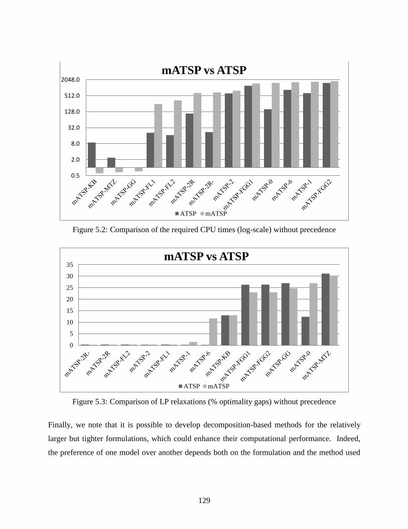
129

Figure 5.2: Comparison of the required CPU times (log-scale) without precedence

Figure 5.3: Comparison of LP relaxations (% optimality gaps) without precedence

Finally, we note that it is possible to develop decomposition-based methods for the relatively

larger but tighter formulations, which could enhance their computational performance. Indeed,

the preference of one model over another depends both on the formulation and the method used

0.5

2.0

8.0

32.0

128.0

512.0

2048.0mATSP vs ATSP

ATSP mATSP

0

5

10

15

20

25

30

35mATSP vs ATSP

ATSP mATSP

130

for its solution, and might differ with an increase in problem size (given more powerful hardware

and an increase in the computational time limit).

5.5. mATSP formulations with special precedence constraints

In this section, we address a precedence constrained multiple traveling salesmen problem in

which a precedence relationship between any specified pair of cities is required to hold only if

both the cities are assigned to the same salesman; otherwise, this relationship is relaxed. We

denote this problem as PCmATSP. In Section 5.6, we shall consider the case of general

precedence relationships, regardless of salesmen (G-PCmATSP). We present various

formulations for the PCmATSP in Subsection 5.5.1 and their computational comparison in

Subsection 5.5.2.

5.5.1 Formulations for PCmATSP

Let be the set of cities that are required to precede city If then we

denote this as We can include the specified special precedence relationships within the

mATSP-MTZ and mATSP-KB models as follows. Note that the -variables determine the

order in which the cities are visited within any tour. This results in the following subtour

elimination and precedence constraints, where we use the (x, z)-variables of Model mATSP-0

along with Constraints (5.6b-g) instead of (5.1b-e) to track the tour of each salesman:

1

1,m

t

i j ij

t

u u q x q

,,...,2, nji ji

(5.26a)

1 ,iu q ni ,...,2

(5.26b)

1 (2 ),t t

i j i ju u q z z ,jPCi ,,...,2 nj mt ,...,1

(5.26c)

0t

jix , ,jPCi ,,...,2 nj .,...,1 mt

(5.26d)

Note that Constraints (5.26a, b) are similar to the subtour elimination Constraints (5.1f, g) in

mATSP-MTZ. Moreover, the precedence constraint (5.26c) ensures that the rank-order of

visiting city is less than that of city j if and only if they are both on the same tour and

otherwise, the constraint is redundant. Constraint (5.26d) ensures that city j does not

131

immediately precede city i on any tour t whenever is required. Thus, we have the

following MTZ precedence-constraint-based formulation for the PCmATSP:

PCmATSP-MTZ: Minimize {(5.6a): (5.6b-g, n, o) and (5.26a-d)}.

Furthermore, the lifted-MTZ constraints (5.2a-c) used in mATSP-KB can be modified as

follows:

1 1

1 1

( 2) 1,m m

t t

i i i

t t

u q x x q

ni ,...,2

(5.27a)

,21

1

1

1

m

t

t

i

m

t

t

ii xxu ni ,...,2

(5.27b)

1 1

( 2) 1,m m

t t

i j ij ji

t t

u u q x q x q

,,...,2, nji .ji

(5.27c)

This yields the following corresponding formulation for the PCmATSP:

PCmATSP-KB: Minimize {(5.6a): (5.6b-g, n, o), (5.26c-d), and (5.27a-c)}.

The formulation of the precedence relationships for the model by Gavish and Graves [55] is

similar to that for the MTZ model, and is given as follows:

,1,2,1

n

ijj

ji

n

ijj

ij ww ni ,...,2

(5.28a)

1

0 ,m

t

ij ij

t

w q x

,,...,2 ni ,,...,1 nj ji

(5.28b)

),2(1,1,1

t

j

t

i

n

jkj

jk

n

ikk

ik zzqww

,jPCi ,,...,2 nj mt ,...,1

(5.28c)

0t

jix , ,jPCi ,,...,2 nj .,...,1 mt

(5.28d)

This leads to the following formulation for the PCmATSP:

PCmATSP-GG: Minimize {(5.6a): (5.6b-g, n, o), and (5.28a-d)}.

The FGG1-based formulation is not able to distinguish between tours and is hence unable to

accommodate the special precedence relationships, but the FGG2-based formulations can do so

because it includes the salesman index t along with the linking z-variables. However, such a

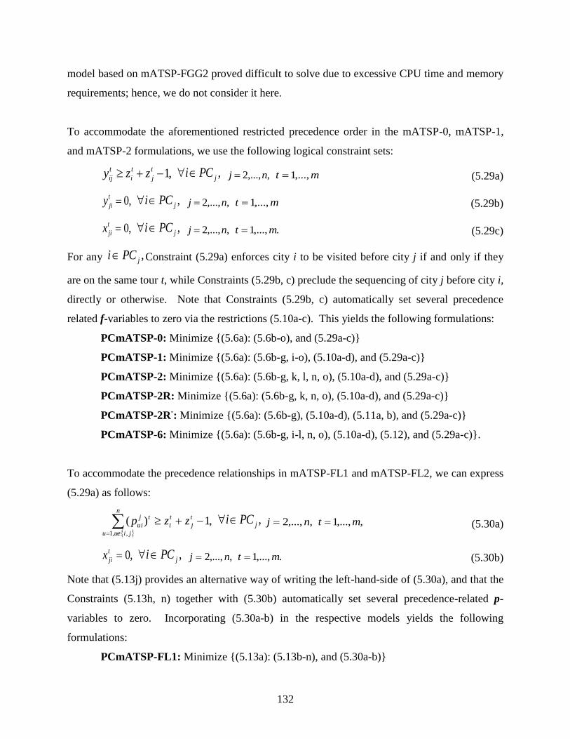
132

model based on mATSP-FGG2 proved difficult to solve due to excessive CPU time and memory

requirements; hence, we do not consider it here.

To accommodate the aforementioned restricted precedence order in the mATSP-0, mATSP-1,

and mATSP-2 formulations, we use the following logical constraint sets:

,1 t

j

t

i

t

ij zzy ,jPCi ,,...,2 nj mt ,...,1 (5.29a)

,0t

jiy ,jPCi ,,...,2 nj mt ,...,1 (5.29b)

,0t

jix ,jPCi ,,...,2 nj .,...,1 mt (5.29c)

For any ,jPCi Constraint (5.29a) enforces city i to be visited before city j if and only if they

are on the same tour t, while Constraints (5.29b, c) preclude the sequencing of city j before city i,

directly or otherwise. Note that Constraints (5.29b, c) automatically set several precedence

related f-variables to zero via the restrictions (5.10a-c). This yields the following formulations:

PCmATSP-0: Minimize {(5.6a): (5.6b-o), and (5.29a-c)}

PCmATSP-1: Minimize {(5.6a): (5.6b-g, i-o), (5.10a-d), and (5.29a-c)}

PCmATSP-2: Minimize {(5.6a): (5.6b-g, k, l, n, o), (5.10a-d), and (5.29a-c)}

PCmATSP-2R: Minimize {(5.6a): (5.6b-g, k, n, o), (5.10a-d), and (5.29a-c)}

PCmATSP-2R-: Minimize {(5.6a): (5.6b-g), (5.10a-d), (5.11a, b), and (5.29a-c)}

PCmATSP-6: Minimize {(5.6a): (5.6b-g, i-l, n, o), (5.10a-d), (5.12), and (5.29a-c)}.

To accommodate the precedence relationships in mATSP-FL1 and mATSP-FL2, we can express

(5.29a) as follows:

,1)(,,1

t

j

t

i

n

jiuu

tj

ui zzp ,jPCi ,,...,2 nj ,,...,1 mt

(5.30a)

,0t

jix ,jPCi ,,...,2 nj .,...,1 mt

(5.30b)

Note that (5.13j) provides an alternative way of writing the left-hand-side of (5.30a), and that the

Constraints (5.13h, n) together with (5.30b) automatically set several precedence-related p-

variables to zero. Incorporating (5.30a-b) in the respective models yields the following

formulations:

PCmATSP-FL1: Minimize {(5.13a): (5.13b-n), and (5.30a-b)}

133

PCmATSP-FL2: Minimize {(5.13a): (5.13b-h, l-n), (5.15a, b), and (5.30a, b)}.

5.5.2 Transformation of PCmATSP to an equivalent PCATSP

In order to develop an equivalent ATSP formulation for the special precedence constrained case,

we need to modify the standard PCATSP to accommodate the set of precedence relationships

defined above. For the MTZ, KB, GG, FGG1, and FGG2 models, it is not possible to

incorporate this precedence order without significantly altering the formulations to distinguish

between tours. Hence, we only consider these precedence relationships within the following

models for the transformed PCATSP: PCATSP-2, PCATSP-2R, PCATSP-2R-, PCATSP-6,

PCATSP-FL1, and PCATSP-FL2.

Recall the definition of the -variable (without the superscript) as used earlier for mATSP-0 in

order to represent the processing sequence between i and j (not necessarily direct). Accordingly,

as before, the transformed model creates m duplicates of the base city, where we

set since is taken as the original base city. We now add

the following constraints to enforce the precedence relationships in the equivalent ATSP

formulations:

{

}

(5.31a)

(5.31b)

For each precedence-restricted pair, Constraint (5.31a) enforces city i to precede city j if and

only if they are on the same tour t, and Constraint (5.31b) prohibits city j to directly precede city

i on any tour t. We thus obtain the following formulations:

PCATSP-0: Minimize {(5.20a): (5.20b-l), and (5.31a, b)}

PCATSP-1: Minimize {(5.20a): (5.20b-e, g-l), (5.21a-c), and (5.31a, b)}

PCATSP-2: Minimize {(5.20a): (5.20b-e, i, k, l), (5.21a-c), and (5.31a, b)}

PCATSP-2R: Minimize {(5.20a): (5.20b-e, k, l), (5.21a-c), (5.22), and (5.31a, b)}

PCATSP-2R-: Minimize {(5.20a): (5.20b-e, k, l), (5.21a-c), and (5.31a, b)}

134

PCATSP-6: Minimize {(5.20a): (5.20b-e, g-i, k, l), (5.21a-c), (5.23), and (5.31a, b)}.

Next, we accommodate the above precedence constraints in the multi-commodity flow-based

formulations PCATSP-FL1 and PCATSP-FL2. We use the flow variables to impose the

following additional constraints:

,

,1

)1(,,2,3

,1

2

1

2

1

,2

1

,2

1

2

1

2

1

,2

1

,2

1

,2

11

22

n

k

j

k

n

k

i

k

n

jkk

jk

n

ikk

ik

n

k

j

k

n

k

i

k

n

jkk

jk

n

ikk

ik

n

ikk

j

ik

mm

tt

tt

pp

mtpppp

pp

p

njPCi j ,,2,

(5.32a)

,'1 1

1

1

1t

t

t

t jj pp ,,...,2 nj ,2,...,1 mt mtt ,...,2'

(5.32b)

.,,2, njPCi j

(5.32c)

Constraint (5.32a) emulates (5.31a), where

ik

ij

j

ik yp . These constraints are used directly for

PCATSP-FL1 given below:

PCATSP-FL1: Minimize {(5.24a): (5.24b-k), and (5.32a-c)}

For the PCATSP-FL2 model, Constraints (5.32a-d) are used while replacing k

ikp with

Rewriting this latter modification as (5.32a-d)+,

we obtain the following formulation:

PCATSP-FL2: Minimize {(5.24a): (5.24b-e, j, k), (5.25a, b), and (5.32a-c)+}.

5.5.3 Computational comparison of various PCmATSP and PCATSP

formulations

For our experimentation, we used two sets of data. The first set consists of three problems from

the TSP Sequential Ordering Problem library [1]: br17.10, esc12, and esc25. The second set of

data consists of three sets of randomly generated problems having 10, 12, 20, and 30 cities,

respectively. The set of randomly generated problems had a varying precedence of low,

medium, and high densities, where we define the precedence density to be the summation of the

135

cardinality of divided by the maximum number of possible precedence

relationships (including implied ones), as follows:

.)2)(1(22

nnPCn

j

j

(5.33)

The precedence densities for the three random test cases were approximately 30%, 50%, and

70%, respectively. Again, these data sets were supplemented with the parameter m to indicate

the number of salesmen available, which was varied from 2-4. The results shown in Tables 5.3

and 5.4, respectively, pertain to the datasets from TSPLIB [1] for the PCmATSP and PCATSP

formulations, where the displayed statistics and highlighting (shading and bold-face) have the

same interpretation as in Tables 5.1 and 5.2. Again, the results for the randomly generated

problems are not included here for the sake of brevity, but are available online as supplementary

data at http://www.sciencedirect.com.

An ordinal ranking of the models in non-decreasing order of average CPU times is as follows:

{PCmATSP-GG, PCmATSP-2R-, PCmATSP-KB, PCmATSP-2R, PCmATSP-2, PCmATSP-

MTZ, PCmATSP-FL2, PCmATSP-FL1, PCATSP-0, PCmATSP-0, PCmATSP-6, PCATSP-2R-,

PCATSP-FL1, PCATSP-2R, PCATSP-FL2, PCmATSP-1, PCATSP-2, PCATSP-1, and

PCATSP-6}. Similar to Figure 5.2, these results are presented in Figure 5.4 to compare the

mATSP and ATSP formulations based on the required CPU times. The flow-based models were

found to be competitive for the br17.10 dataset, although the mATSP-MTZ and mATSP-KB

models required the least CPU times and peak memory, and were the fastest on average. As

mentioned in the previous section, the advantage of these models lies in the simplicity of their

formulations; however, they produce weak LP relaxations and consequently enumerate a

relatively greater number of branch-and-bound nodes. For example, the number of nodes

generated for br17.10 using the PCmATSP-MTZ formulation were 290,726 , 123,457

, and 23,617 , while those generated by PCATSP-FL2 were 1,702, 1,104, and

15, respectively, for these instances.

136

Table 5.3: Comparison of the PCmATSP models

Test

Problem Measure

PCmATSP

-MTZ

PCmATSP

-KB

PCmATSP

-GG

PCmATSP

-0

PCmATSP

-1

PCmATSP

-2

PCmATSP

-2R

PCmATSP

-2R-

PCmATSP

-6

PCmATSP

-FL1

PCmATSP

-FL2

esc12 ZLP 6.52 18.60 8.04 17.16 27.00 27.00 27.00 28.47 28.47 28.40 28.40 m=2 %Gap 82.84 51.05 78.85 54.84 28.95 28.95 28.95 25.09 25.09 25.26 25.26

Sol’n CPU-LP 0.08 0.21 0.07 0.14 19.28 3.88 1.57 2.12 7.69 2.49 2.18

38 CPU-MIP 430.36 70.47 485.14 1711.50 1742.50 507.91 429.24 375.96 1306.46 1072.82 935.41

# of Nodes 290726 54678 96103 4935 176 452 484 693 177 2347 1702

esc12 ZLP 9.64 20.70 11.25 17.17 25.00 25.00 25.00 25.15 25.15 26.50 26.50

m=3 %Gap 70.78 37.27 65.90 47.97 24.24 24.24 24.24 23.79 23.79 19.70 19.70 Sol’n CPU-LP 0.10 0.09 0.07 0.17 26.93 5.69 7.10 3.07 11.35 4.70 3.16

33 CPU-MIP 271.21 173.57 838.10 3600.00 3153.10 525.31 490.72 512.69 3600.00 1131.48 979.60

# of Nodes 123457 50105 147385 1581 186 202 234 373 308 1409 1101

Incumbent

33.00

33.00

esc12 ZLP 12.78 23.70 14.50 19.18 25.00 25.00 25.00 25.16 25.16 26.60 26.60

m=4 %Gap 58.76 23.55 53.23 38.13 19.35 19.35 19.35 18.84 18.84 14.19 14.19 Sol’n CPU-LP 0.10 0.07 0.07 0.31 25.77 7.05 7.92 7.49 14.79 6.14 4.13

31 CPU-MIP 76.97 123.47 97.06 3600.00 3600.00 327.19 198.06 195.93 2596.32 123.90 25.50

# of Nodes 23617 25337 16550 984 76 102 96 79 81 25 15

Incumbent

31.00 31.00

br17.10 ZLP 1069.09 1209.00 1084.50 1209.89 1257.00 1257.00 1257.00 1257.00 1257.00 1210.71 1210.71

m=2 %Gap 15.82 4.80 14.61 4.73 1.02 1.02 1.02 1.02 1.02 4.67 4.67 Sol’n CPU-LP 0.08 0.06 0.06 0.09 0.63 0.43 0.30 0.30 0.87 0.31 0.22

1270 CPU-MIP 0.14 0.14 1.15 2.49 3.16 1.53 0.74 0.78 2.82 1.26 1.25

# of Nodes 183 266 827 67 3 2 0 0 0 14 18

br17.10 ZLP 901.80 1015.50 900.09 1015.50 1020.00 1020.00 1020.00 1020.00 1020.00 1015.50 1015.50

m=3 %Gap 11.67 0.54 11.84 0.54 0.10 0.10 0.10 0.10 0.10 0.54 0.54

Sol’n CPU-LP 0.08 0.08 0.06 0.13 1.15 0.45 0.31 0.64 0.99 0.40 0.28 1021 CPU-MIP 0.11 0.08 0.37 0.77 4.55 2.90 1.29 1.51 20.71 1.61 0.84

# of Nodes 15 0 238 0 0 0 0 5 9 0 0

br17.10 ZLP 748.89 822.00 747.00 822.00 822.00 822.00 822.00 822.00 822.00 822.00 822.00

m=4 %Gap 8.89 0.00 9.12 0.00 0.00 0.00 0.00 0.00 0.00 0.00 0.00

Sol’n CPU-LP 0.11 0.06 0.10 0.15 1.26 0.41 0.44 0.27 0.93 0.49 0.51

822 CPU-MIP 0.05 0.05 0.27 0.42 2.06 0.86 0.65 0.97 2.37 0.76 0.37 # of Nodes 0 0 115 0 0 0 0 0 0 0 0

esc25 ZLP 1069.19 1068.54 1075.20 1053.00 1159.08 1159.08 1159.08 1159.08 1159.08 1141.00 1141.00

m=2 %Gap 8.07 8.12 7.55 9.46 0.34 0.34 0.34 0.34 0.34 1.89 1.89

Sol’n CPU-LP 0.08 0.06 0.10 0.58 962.36 15.56 12.64 12.12 209.97 8.92 7.58

1163 CPU-MIP 1.45 0.32 10.14 8.35 2607.97 40.09 23.63 24.23 809.86 30.09 48.00

# of Nodes 546 49 3298 54 0 0 0 0 0 5 7 esc25 ZLP 908.96 908.79 910.42 905.00 969.50 969.50 969.50 969.50 969.50 943.00 943.00

m=3 %Gap 7.25 7.27 7.10 7.65 1.07 1.07 1.07 1.07 1.07 3.78 3.78

Sol’n CPU-LP 0.18 0.07 0.10 1.79 1314.25 20.42 42.38 15.66 739.61 12.65 10.01

980 CPU-MIP 0.76 0.46 2.62 31.76 3600.00 30.47 37.71 43.94 2264.51 59.51 33.71

# of Nodes 171 151 409 188 0 0 0 0 3 7 0

Incumbent

121.00

esc25 ZLP 765.68 765.35 766.91 758.00 821.50 821.50 821.50 821.50 821.50 795.00 795.00

m=4 %Gap 7.97 8.01 7.82 8.89 1.26 1.26 1.26 1.26 1.26 4.45 4.45

Sol’n CPU-LP 0.11 0.09 0.12 1.49 2737.22 59.69 49.78 38.00 1996.80 17.08 17.09

832 CPU-MIP 0.86 0.72 3.64 572.94 3600.00 64.13 37.65 57.69 3600.00 63.83 107.87

# of Nodes 174 239 560 447 0 0 0 0 0 23 19

Incumbent

* 4238.00

Averag

e

ZLP 167.47 178.55 168.26 177.47 212.71 187.08 192.89 187.14 212.77 183.35 183.35 %Gap 33.95 20.18 32.55 33.02 6.12 7.00 6.80 6.65 5.78 15.80 15.80

CPU-LP 0.12 0.09 0.09 0.40 797.97 192.24 213.46 173.05 682.23 16.21 11.34

CPU-MIP 738.09 549.54 483.78 1164.42 1428.02 714.63 645.44 517.41 1289.98 903.45 814.92

# of Nodes 147083 248785 62325 500 24 42 47 55 38 293 255

Min ZLP 0.60 0.85 0.64 0.85 1.03 1.03 1.03 1.03 1.03 0.87 0.87 %Gap 4.68 0.00 4.86 0.00 0.00 0.00 0.00 0.00 0.00 0.00 0.00

CPU-LP 0.01 0.05 0.05 0.05 0.08 0.06 0.05 0.05 0.08 0.09 0.07

CPU-MIP 0.02 0.04 0.11 0.14 0.08 0.05 0.04 0.05 0.09 0.08 0.06

# of Nodes 0 0 0 0 0 0 0 0 0 0 0

Max ZLP 1069.19 1209.00 1084.50 1209.89 1257.00 1257.00 1257.00 1257.00 1257.00 1210.71 1210.71

%Gap 82.84 56.74 78.85 64.54 28.95 37.82 37.82 37.82 25.09 56.74 56.74 CPU-LP 0.31 0.44 0.26 1.79 3600.00 3093.72 3600.00 2675.28 3600.00 187.99 116.18

CPU-MIP 3600.00 3600.00 3600.00 3600.00 3600.00 3600.00 3600.00 3600.00 3600.00 3600.00 3600.00

# of Nodes 1006309 2645491 610879 4935 193 452 484 693 309 2347 2019

* No feasible solution found within 3,600 seconds of CPU time

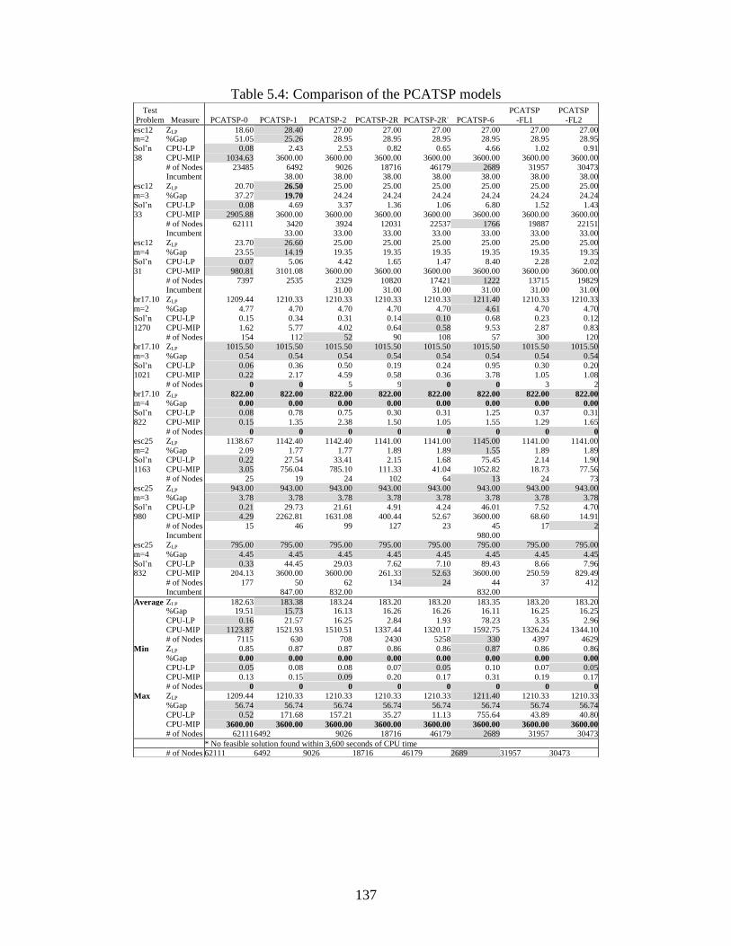
137

Table 5.4: Comparison of the PCATSP models

Test

Problem Measure PCATSP-0 PCATSP-1 PCATSP-2 PCATSP-2R PCATSP-2R- PCATSP-6

PCATSP

-FL1

PCATSP

-FL2

esc12 ZLP 18.60 28.40 27.00 27.00 27.00 27.00 27.00 27.00 m=2 %Gap 51.05 25.26 28.95 28.95 28.95 28.95 28.95 28.95

Sol’n CPU-LP 0.08 2.43 2.53 0.82 0.65 4.66 1.02 0.91

38 CPU-MIP 1034.63 3600.00 3600.00 3600.00 3600.00 3600.00 3600.00 3600.00

# of Nodes 23485 6492 9026 18716 46179 2689 31957 30473 Incumbent 38.00 38.00 38.00 38.00 38.00 38.00 38.00

esc12 ZLP 20.70 26.50 25.00 25.00 25.00 25.00 25.00 25.00

m=3 %Gap 37.27 19.70 24.24 24.24 24.24 24.24 24.24 24.24

Sol’n CPU-LP 0.08 4.69 3.37 1.36 1.06 6.80 1.52 1.43

33 CPU-MIP 2905.88 3600.00 3600.00 3600.00 3600.00 3600.00 3600.00 3600.00

# of Nodes 62111 3420 3924 12031 22537 1766 19887 22151 Incumbent 33.00 33.00 33.00 33.00 33.00 33.00 33.00

esc12 ZLP 23.70 26.60 25.00 25.00 25.00 25.00 25.00 25.00

m=4 %Gap 23.55 14.19 19.35 19.35 19.35 19.35 19.35 19.35

Sol’n CPU-LP 0.07 5.06 4.42 1.65 1.47 8.40 2.28 2.02

31 CPU-MIP 980.81 3101.08 3600.00 3600.00 3600.00 3600.00 3600.00 3600.00

# of Nodes 7397 2535 2329 10820 17421 1222 13715 19829 Incumbent 31.00 31.00 31.00 31.00 31.00 31.00

br17.10 ZLP 1209.44 1210.33 1210.33 1210.33 1210.33 1211.40 1210.33 1210.33

m=2 %Gap 4.77 4.70 4.70 4.70 4.70 4.61 4.70 4.70

Sol’n CPU-LP 0.15 0.34 0.31 0.14 0.10 0.68 0.23 0.12

1270 CPU-MIP 1.62 5.77 4.02 0.64 0.58 9.53 2.87 0.83

# of Nodes 154 112 52 90 108 57 300 120 br17.10 ZLP 1015.50 1015.50 1015.50 1015.50 1015.50 1015.50 1015.50 1015.50

m=3 %Gap 0.54 0.54 0.54 0.54 0.54 0.54 0.54 0.54

Sol’n CPU-LP 0.06 0.36 0.50 0.19 0.24 0.95 0.30 0.20

1021 CPU-MIP 0.22 2.17 4.59 0.58 0.36 3.78 1.05 1.08

# of Nodes 0 0 5 9 0 0 3 2

br17.10 ZLP 822.00 822.00 822.00 822.00 822.00 822.00 822.00 822.00 m=4 %Gap 0.00 0.00 0.00 0.00 0.00 0.00 0.00 0.00

Sol’n CPU-LP 0.08 0.78 0.75 0.30 0.31 1.25 0.37 0.31

822 CPU-MIP 0.15 1.35 2.38 1.50 1.05 1.55 1.29 1.65

# of Nodes 0 0 0 0 0 0 0 0

esc25 ZLP 1138.67 1142.40 1142.40 1141.00 1141.00 1145.00 1141.00 1141.00

m=2 %Gap 2.09 1.77 1.77 1.89 1.89 1.55 1.89 1.89 Sol’n CPU-LP 0.22 27.54 33.41 2.15 1.68 75.45 2.14 1.90

1163 CPU-MIP 3.05 756.04 785.10 111.33 41.04 1052.82 18.73 77.56

# of Nodes 25 19 24 102 64 13 24 73

esc25 ZLP 943.00 943.00 943.00 943.00 943.00 943.00 943.00 943.00

m=3 %Gap 3.78 3.78 3.78 3.78 3.78 3.78 3.78 3.78

Sol’n CPU-LP 0.21 29.73 21.61 4.91 4.24 46.01 7.52 4.70 980 CPU-MIP 4.29 2262.81 1631.08 400.44 52.67 3600.00 68.60 14.91

# of Nodes 15 46 99 127 23 45 17 2

Incumbent

980.00

esc25 ZLP 795.00 795.00 795.00 795.00 795.00 795.00 795.00 795.00

m=4 %Gap 4.45 4.45 4.45 4.45 4.45 4.45 4.45 4.45

Sol’n CPU-LP 0.33 44.45 29.03 7.62 7.10 89.43 8.66 7.96 832 CPU-MIP 204.13 3600.00 3600.00 261.33 52.63 3600.00 250.59 829.49

# of Nodes 177 50 62 134 24 44 37 412

Incumbent 847.00 832.00

832.00

Average ZLP 182.63 183.38 183.24 183.20 183.20 183.35 183.20 183.20 %Gap 19.51 15.73 16.13 16.26 16.26 16.11 16.25 16.25

CPU-LP 0.16 21.57 16.25 2.84 1.93 78.23 3.35 2.96 CPU-MIP 1123.87 1521.93 1510.51 1337.44 1320.17 1592.75 1326.24 1344.10

# of Nodes 7115 630 708 2430 5258 330 4397 4629

Min ZLP 0.85 0.87 0.87 0.86 0.86 0.87 0.86 0.86

%Gap 0.00 0.00 0.00 0.00 0.00 0.00 0.00 0.00

CPU-LP 0.05 0.08 0.08 0.07 0.05 0.10 0.07 0.05

CPU-MIP 0.13 0.15 0.09 0.20 0.17 0.31 0.19 0.17 # of Nodes 0 0 0 0 0 0 0 0

Max ZLP 1209.44 1210.33 1210.33 1210.33 1210.33 1211.40 1210.33 1210.33

%Gap 56.74 56.74 56.74 56.74 56.74 56.74 56.74 56.74

CPU-LP 0.52 171.68 157.21 35.27 11.13 755.64 43.89 40.80

CPU-MIP 3600.00 3600.00 3600.00 3600.00 3600.00 3600.00 3600.00 3600.00

# of Nodes 62111 6492 9026 18716 46179 2689 31957 30473

* No feasible solution found within 3,600 seconds of CPU time

# of Nodes 62111 6492 9026 18716 46179 2689 31957 30473

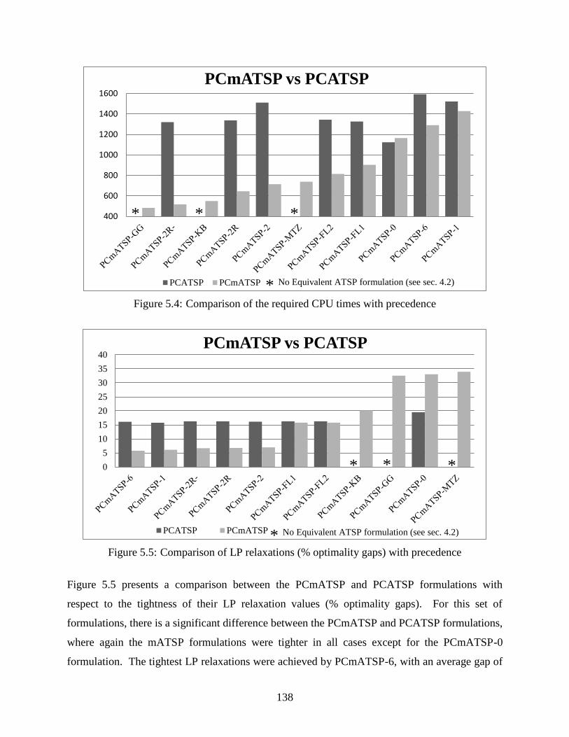
138

Figure 5.4: Comparison of the required CPU times with precedence

Figure 5.5: Comparison of LP relaxations (% optimality gaps) with precedence

Figure 5.5 presents a comparison between the PCmATSP and PCATSP formulations with

respect to the tightness of their LP relaxation values (% optimality gaps). For this set of

formulations, there is a significant difference between the PCmATSP and PCATSP formulations,

where again the mATSP formulations were tighter in all cases except for the PCmATSP-0

formulation. The tightest LP relaxations were achieved by PCmATSP-6, with an average gap of

400

600

800

1000

1200

1400

1600

PCmATSP vs PCATSP

PCATSP PCmATSP

0

5

10

15

20

25

30

35

40PCmATSP vs PCATSP

PCATSP PCmATSP

* * *

* No Equivalent ATSP formulation (see sec. 4.2)

* No Equivalent ATSP formulation (see sec. 4.2)

* * *

139

5.78% from the integer optimal solution at the root node. The PCmATSP-KB, PCmATSP-GG,

PCmATSP-0, and PCmATSP-MTZ formulations displayed the weakest relaxations, yielding an

average percentage optimality gap value of 20.18, 32.55, 33.02, and 33.95%, respectively.

Again, the PCmATSP-FL1, PCmATSP-FL2, PCmATSP-1, and PCmATSP-2 models were

encumbered by a relatively large number of variables and constraints. Also, generally speaking,

the models having higher precedence densities required less CPU times when compared with the

same formulations having a lower precedence density.

A comparison of the performances of the PCmATSP models with the equivalent PCATSP

formulations reveals that the required CPU times were smaller for all the PCmATSP

formulations compared with the PCATSP formulations, with the exception of PCmATSP-0. The

LP relaxations of the PCmATSP formulations were found to be tighter than those for the

transformed formulations, with the exception that PCATSP-0 yielded tighter relaxations than

PCmATSP-0. Hence, due to tighter LP relaxations and smaller CPU times, the PCmATSP

models turned out to be generally more robust and effective, and are therefore preferable over the

equivalent PCATSP formulations. This result further reinforces the finding in [56, 86, 140] for

similarly transformed reformulations.

5.6. mATSP formulations with general precedence constraints

In this section, we consider the general precedence constrained mATSP, where the specified

precedence order among pairs of cities is enforced even when the cities in a pair belong to tours

of different salesmen. In this context, the -value is interpreted as the transition time from i to j

(including the processing time for node i, as necessary), so that the precedence relationship is

based on the times of visit for the different nodes and is accommodated by tracking the travel

time of each salesman and then ensuring that the precedence holds even when the restricted cities

in any pair are visited by different salesmen. Accordingly, in lieu of the u-variables that

previously represented the rank-order of visiting the cities, we utilize a variable to denote the

time of visiting city j (or the start-time for j), where . Note that this problem has a job

shop-type setting where jobs cannot be processed until the processors are available.

140

5.6.1 Formulations for G-PCmATSP

To model this general type of precedence relationship, we modify the foregoing model’s

constraints to further accommodate the new -variables, where with

jL and jU representing the earliest and the latest possible times for visiting city j. For

convenience, we also define noting that Note that the - and -values

might either be prespecified according to certain user-based considerations, or might be simply

computed given an upper bound on the length of a tour and a precedence tree. For example, we

can compute the - and -values as follows, where we let denote the set of cities that

succeed city (i.e., for which j is a predecessor), :

{

{ }

{ }}

{

{ } }

where equals some known upper bound on the total processing time over all salesmen (which

could be updated during the branch-and-bound process), minus minus the

smallest -values, and minus the smallest -values, . It is readily seen

that for general -values, we must have or else the total processing time would exceed

the specified upper bound. For our implementation, we let this upper bound equal the sum of the

highest cost parameters, and for simplicity, we do not update it during the branch-

and-bound process.

The objective function is modified accordingly to consider the total cost of travel between cities,

as well as the cost accrued due to slack time, where these two components are treated as primary

and secondary measures, respectively. This is achieved by the use of a multiplier as follows:

Minimize ,21 ,1 1

n

j

j

n

i

n

ijj

m

t

t

ijij xc

where (5.34a)

.

)(1

1

2

n

j

jj LU

(5.34b)

141

The objective function (5.34a) minimizes the total cost of travel (total sum of transition times)

with a preemptive priority, and among alternative optimal solutions, it minimizes the sum of visit

times (to make the -values as tightly packed as possible). Using the result of Sherali and

Soyster [127], this is achieved by selecting as in (5.34b), where the denominator exceeds the

difference between the maximum and minimum possible values of the secondary objective

functions, noting that the first priority objective function is integer-valued (assuming integral c-

parameters).

The relevant constraints that serve to enforce the general precedence relationship within the G-

mATSP models can thus be stated as follows:

,11

m

t

t

ijijijijji xULcc ,,...,1 ni ,,...,2 nj ji

(5.35a)

,ji ,jPCi nj ,...,2

(5.35b)

;01 ,0t

jix ,jPCi ,,...,2 nj ;,...,1 mt and

,0t

ijx if ,jiji UcL

,,...,1 ni ,,...,2 nj ,ji .,...,1 mt (5.35c)

Constraint (5.35a) ensures the proper accounting of time from city i to city j, given that this

transition occurs for some salesman. Constraint (5.35b) asserts the required precedence order.

Note that for any , if are processed by different salesmen, it is possible to have

, as for example if the settings required to commence job on any machine are contingent

on what settings (tolerances, manufacturing protocols, etc.) are established for job at the start of

its processing, whence a near-concurrent start for jobs is possible. Alternatively, we

could model (5.35b) by including some positive slack on the left-hand-side of this

restriction. Finally, Constraint (5.35c) enforces logical requirements for the - and -variables.

Furthermore, we can impose the lifted valid inequalities (5.35d) established by Proposition 1

below:

142

Proposition 1. The following inequality is valid for G-PCmATSP:

{ }

m

t

t

jx1

1

(

m

t

t

jx1

1 ) { { }

{ } { }

{ }} (5.35d)

Proof. Consider any { } If t

jx1 for any then (5.35d) asserts that

{ } which holds true. Otherwise, suppose that 01 t

jx , In this

case, on any tour containing city j, there must exist at least one intervening city between the base

city 1 and city j, whence we must have { }

{ } { }

{ } where we do not

necessarily assume the triangular inequality to hold true for the c-parameters. Noting that we

also have (5.35d) therefore holds true.

By replacing Constraints (5.26a-c) with (5.35a-d), we obtain the following MTZ-based

formulation for the G-PCmATSP:

G-PCmATSP-MTZ: Minimize {(5.34a): (5.6b-g, n, o), and (5.35a-d)}.

The PCmATSP-GG model can be extended to the present case by adding Constraints (5.35a-d)

as follows:

G-PCmATSP-GG: Minimize {(5.34a): (5.6b-g, n, o), (5.28a-d), and (5.35a-d)}.

For the FGG1-based model, we include Constraints (5.36b-e) stated below similar to (5.35a-d),

with the exception that the r-variables are summed over the ranking index much like the

summation over the tour index in the MTZ formulation:

G-PCmATSP-FGG1: Minimize

n

j

j

n

i

n

ijj

q

k

ijkijrc21 ,1 0

(5.36a)

subject to (5.5b-g), plus

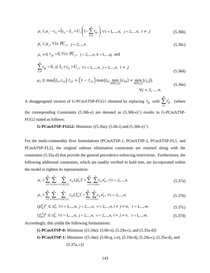
143

,10

q

k

ijkijijijji rULcc ,,...,1 ni ,,...,2 nj ji

(5.36b)

,ji ,jPCi nj ,...,2

(5.36c)

;01 ,0jikr ,jPCi ,,...,2 nj ;,...,1 qk and

,00

q

k

ijkr if ,jiji UcL

,,...,1 ni ,,...,2 nj ji

(5.36d)

{ } 01 jr ( 01 jr ) { { }

{ } { }

{ }}

(5.36e)

A disaggregated version of G-PCmATSP-FGG1 obtained by replacing ijkr with 1

mt

ijk

t

r

(where

the corresponding Constraints (5.36b-e) are denoted as (5.36b-e)+) results in G-PCmATSP-

FGG2 stated as follows:

G-PCmATSP-FGG2: Minimize {(5.36a): (5.6b-i) and (5.36b-e)+}.

For the multi-commodity flow formulations (PCmATSP-1, PCmATSP-2, PCmATSP-FL1, and

PCmATSP-FL2), the original subtour elimination constraints are retained along with the

constraints (5.35a-d) that provide the general precedence enforcing restrictions. Furthermore, the

following additional constraints, which are readily verified to hold true, are incorporated within

the model to tighten its representation:

,)(1 ,1 ,,2 1 ,1

m

t

n

ikk

n

kill

m

t

n

ikk

t

kiki

ti

klkli xcpc ni ,...,2

(5.37a)

,)(1 ,1 ,,2 1 ,1

m

t

n

ikk

n

kill

m

t

n

ikk

t

kiki

tl

kikli xcfc .,...,2 ni

(5.37b)

,,...,1 ni ,,...,2 nj ,,...,2 nv ,uji mt ,...,1

(5.37c)

,,...,1 ni ,,...,2 nj ,,...,2 nv ,vji .,...,1 mt

(5.37d)

Accordingly, this yields the following formulations:

G-PCmATSP-0: Minimize {(5.34a): (5.6b-o), (5.29a-c), and (5.35a-d)}

G-PCmATSP-1: Minimize {(5.34a): (5.6b-g, i-o), (5.10a-d), (5.29a-c), (5.35a-d), and

(5.37a, c)}

144

G-PCmATSP-2: Minimize {(5.34a): (5.6b-g, k, l, n, o), (5.10a-d), (5.29a-c), (5.35a-d),

and (5.37a, c)}

G-PCmATSP-2R: Minimize {(5.34a): (5.6b-g, k, n, o), (5.10a-d), (5.29a-c), (5.35a-d),

and (5.37a, c)}

G-PCmATSP-2R-: Minimize {(5.34a): (5.6b-g, n, o), (5.10a-d), (5.11a, b), (5.29a-c),

(5.35a-d), and (5.37a, c)}

G-PCmATSP-6: Minimize {(5.34a): (5.6b-g, i-l, n, o), (5.10a-d), (5.12), (5.29a-c),

(5.35a-d), and (5.37a, c)}

G-PCmATSP-FL1: Minimize {(5.34a): (5.13b-n), (5.30a-b), (5.35a-d), and (5.37b, d)}

G-PCmATSP-FL2: Minimize {(5.34a): (5.13b-h, l-n), (5.15a, b), (5.30a, b), (5.35a-d),

and (5.37b, d)}.

5.6.2 Transformation of G-PCmATSP to an equivalent G-PCATSP

An objective function similar to that in (5.34a) is used for the transformed G-PCATSP model

formulation, as specified below, where the value of is given by (5.34b):

Minimize .21 ,11 1

n

j

j

n

i

n

ijj

ijij xc

(5.38)

The formulations for the transformed G-PCATSP can be obtained by using the MTZ subtour

elimination constraints similar to (5.35a-d). Note that this formulation is different from the

standard MTZ model representation in that the -variables are reset whenever the tour returns to

a duplicate of the base city. The following constraints account for the tracking of time along the

tours for the general precedence case:

,1 ijijijijji xULcc

,,...,2,1,...,11 ni m ,,...,2 nj ji

(5.39a)

,ji ,jPCi nj ,...,2

(5.39b)

,01 t

;,...,1 mt ,0jix ,jPCi ;,...,2 nj and

,0ijx if ,jiji UcL

,,...2,1,...,11 ni m ,,...,2 nj ji (5.39c)

145

{ }

m

t

jtx

1

1

(

m

t

jtx

1

1 ) { { }

{ } { }

{ }} (5.39d)

This yields the modified MTZ-based formulation as follows:

G-PCATSP-MTZ: Minimize {(5.38): (5.16b-d, h), and (5.39a-d)}.

Likewise, for each of the models below, the original subtour elimination constraints are retained

and are further augmented by the constraints (5.39a-d) that provide the general precedence

enforcing relationships:

G-PCATSP-GG: Minimize {(5.38): (5.16b-d, h), (5.18a-c), and (5.39a-d)}.

G-PCATSP-0: Minimize {(5.38): (5.20b-l), (5.31a, b), and (5.39a-d)}.

G-PCATSP-1: Minimize {(5.38): (5.20b-e, g-l), (5.21a-c), (5.31a, b), and (5.39a-d)}.

G-PCATSP-2: Minimize {(5.38): (5.20b-e, i, k, l), (5.21a-c), (5.31a, b), and (5.39a-d)}.

G-PCATSP-2R: Minimize {(5.38): (5.20b-e, k, l), (5.21a-c), (5.22), (5.31a, b), and

(5.39a-d)}.

G-PCATSP-2R-: Minimize {(5.38): (5.20b-e, k, l), (5.21a-c), (5.31a, b), and (5.39a-d)}.

G-PCATSP-6: Minimize {(5.38): (5.20b-e, g-i, k, l), (5.21a-c), (5.23), (5.31a, b), and

(5.39a-d)}.

G-PCATSP-FL1: Minimize {(5.38): (5.24b-k), (5.32a-c), and (5.39a-d)}.

G-PCATSP-FL2: Minimize {(5.38): (5.24b-e, j, k), (5.25a, b), (5.32a-c) +

,

and (5.39a-d)}.

Additionally, the FGG1-based model and its FGG2-type relaxation are obtained by using the

constraints (5.19b-g) along with (5.36b-d) rewritten by replacing q with q' (denoted (5.36b-d)'),

and the following modification of Constraint (5.36e):

{ }

m

t

q

k

jktr

1

'

0

1

(

m

t

q

k

jktr

1

'

0

1 ) { { }

{ } { }

{ }} (5.40)

146

This yields the following formulations for the FGG-1-based model and its FGG2-type relaxation:

G-PCATSP-FGG1: Minimize {(5.36a): (5.19b-h), (5.36b-d)', and (5.40)}.

G-PCATSP-FGG2: Minimize {(5.36a): (5.19b, c, e-h), (5.36b-d)', and (5.40)}.

5.6.3 Computational comparison of various G-PCmATSP and G-PCATSP

formulations

Computational experiments were conducted for the generalized precedence models using the

same datasets that were utilized for the special precedence problems. The number of traveling

salesmen and the specified precedence order were varied in the same fashion as that for the

PCmATSP formulations.

The results of our computational experimentation with the generalized precedence models are

presented in Tables 5.5 and 5.6, where the legend and statistics displayed, including the shaded

and bold-faced highlighting, are the same as for Tables 5.1 and 5.2. Based on these results, an

ordinal ranking of the models in non-decreasing order of average CPU times is as follows: {G-

PCATSP-MTZ, G-PCATSP-GG, G-PCmATSP-GG, G-PCmATSP-MTZ, G-PCATSP-0, G-

PCmATSP-0, G-PCmATSP-2R, G-PCmATSP-2R-, G-PCATSP-FL1, G-PCATSP-2R

-, G-

PCATSP-FL2, G-PCATSP-2R, G-PCmATSP-2, G-PCmATSP-FGG1, G-PCmATSP-6, G-

PCATSP-FGG1, G-PCATSP-2, G-PCmATSP-FL2, G-PCmATSP-FL1, G-PCATSP-1, G-

PCATSP-6, G-PCmATSP-1, G-PCmATSP-FGG2, and G-PCATSP-FGG2}. Figure 5.6

emulates Figures 5.2 and 5.4 for a comparison of the CPU times for the corresponding mATSP

and ATSP formulations. As can be seen from Figure 5.6, the G-PCATSP formulations were

solved faster than the G-PCmATSP formulations for the GG, MTZ, ATSP-0, FL2, and FL1

models. However, as evident from Figure 5.7, the G-PCmATSP formulations produced tighter

LP relaxations than the G-PCATSP formulations for all the models except for the mATSP-0

formulation. It is worth noting that G-PCATSP-MTZ and G-PCATSP-GG were the only

formulations that were able to solve all the problem instances. The level of precedence in the

data affected the results in a similar fashion as for the special precedence case. Generally,

problems having a high precedence density were relatively easier to solve, while those having

medium precedence densities proved to be the most difficult to solve.

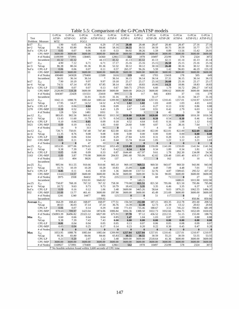
147

Table 5.5: Comparison of the G-PCmATSP models

Test

Problem Measure

G-PCm

ATSP-

MTZ

G-PCm

ATSP-GG

G-PCm

ATSP-

FGG1

G-PCm

ATSP-FGG2

G-PCm

ATSP-0

G-PCm

ATSP-1

G-PCm

ATSP-2

G-PCm

ATSP-2R

G-PCm

ATSP-2R-

G-PCm

ATSP-6

G-PCm

ATSP-FL1

G-PCm

ATSP-FL2

br17 ZLP 1.90 6.65 6.29 6.29 17.16 28.48 28.48 28.47 28.40 28.47 27.16 27.16 m=2 %Gap 95.36 83.80 84.66 84.66 58.16 30.55 30.55 30.59 30.75 30.59 33.77 33.77

Sol’n CPU-LP 0.05 0.07 0.06 0.10 0.33 84.92 38.26 1.59 0.89 13.56 15.42 26.01 38 CPU-MIP 3600.00 3600.00 3600.00 3600.00 3600.00 3600.00 3600.00 3600.00 3600.00 3600.00 3600.00 3600.00

# of Nodes 1109399 573991 138405 54360 12861 512 1978 10497 25199 578 2324 3072

Incumbent 41.12 41.12 * 44.13 41.12 41.13 41.12 41.13 42.11 41.14 41.13 41.14

br17 ZLP 4.90 7.12 6.71 6.71 17.17 25.16 25.16 25.15 26.50 25.15 25.16 25.16

m=3 %Gap 86.38 80.24 81.36 81.36 52.32 30.12 30.12 30.16 26.40 30.16 30.12 30.12

Sol’n CPU-LP 0.06 0.06 0.07 0.11 0.57 265.37 96.26 5.59 1.42 96.83 46.19 155.19 33 CPU-MIP 3600.00 3600.00 3600.00 3600.00 3600.00 3600.00 3600.00 3600.00 3600.00 3600.00 3600.00 3600.00

# of Nodes 690480 343028 170400 13588 1616 119 602 1703 13418 178 505 649

Incumbent 36.01 36.14 36.14 * 36.14 36.15 36.14 36.14 37.31 36.15 36.14 36.15

br17 ZLP 7.90 10.19 9.97 9.97 19.18 25.17 25.17 25.16 26.60 25.16 25.17 25.17

m=4 %Gap 74.51 67.14 67.85 67.85 38.14 18.83 18.83 18.86 14.21 18.86 18.83 18.83

Sol’n CPU-LP 0.06 0.07 0.07 0.13 0.67 560.75 279.01 6.60 1.79 16.72 286.27 147.63 31 CPU-MIP 2528.89 518.38 3600.00 3600.00 3600.00 3600.00 2024.23 3600.00 3390.62 3600.00 3600.00 3600.00

# of Nodes 504387 22428 131551 23418 999 5 117 845 4303 37 116 279

Incumbent

31.01 31.01 31.16 81.19 31.17 31.16 34.17 31.16

esc12 ZLP 1042.13 1088.78 1085.64 1085.64 1209.90 1257.04 1257.04 1257.01 1210.45 1257.01 1210.97 1210.97

m=2 %Gap 17.95 14.27 14.52 14.52 4.74 1.02 1.02 1.03 4.69 1.03 4.65 4.65

Sol’n CPU-LP 0.05 0.06 0.04 0.06 0.09 2.67 1.45 0.27 0.13 0.92 0.86 0.88 1270 CPU-MIP 0.28 0.52 3.92 6.43 1.29 6.67 3.68 0.91 0.42 2.79 6.03 3.13

# of Nodes 128 524 1481 1031 31 5 3 0 45 3 58 14

esc12 ZLP 883.85 902.56 900.62 900.62 1015.50 1020.00 1020.00 1020.00 1015.50 1020.00 1016.30 1016.30

m=3 %Gap 13.43 11.60 11.79 11.79 0.54 0.10 0.10 0.10 0.54 0.10 0.46 0.46

Sol’n CPU-LP 0.10 0.06 0.05 0.09 0.18 4.52 4.64 0.45 0.16 1.08 1.12 0.42

1021 CPU-MIP 0.09 0.19 0.82 1.85 0.60 24.60 9.80 4.87 1.26 38.16 7.64 1.77 # of Nodes 14 9 313 90 0 5 7 4 10 3 6 0

esc12 ZLP 728.71 750.01 747.40 747.40 822.00 822.00 822.00 822.00 822.01 822.00 822.69 822.69

m=4 %Gap 11.35 8.76 9.08 9.08 0.00 0.00 0.00 0.00 0.00 0.00 0.00 0.00

Sol’n CPU-LP 0.01 0.06 0.04 0.08 0.29 27.84 6.93 0.31 0.28 1.33 4.20 3.47

822 CPU-MIP 0.05 0.11 0.34 1.41 0.44 15.74 10.44 1.05 1.22 3.12 3.21 1.83

# of Nodes 0 0 47 10 0 0 0 0 0 0 0 0 esc25 ZLP 1053.95 1077.06 1076.62 1076.62 1053.49 1159.09 1159.09 1159.09 1141.00 1159.09 1141.94 1141.94

m=2 %Gap 9.38 7.39 7.43 7.43 9.42 0.34 0.34 0.34 1.89 0.34 1.81 1.81

Sol’n CPU-LP 0.05 0.08 0.09 0.33 0.87 1644.40 417.97 9.61 1.78 262.30 134.08 54.36

1163 CPU-MIP 0.89 3.87 770.98 3600.00 204.93 2981.68 705.06 42.82 128.48 1101.40 419.17 474.30

# of Nodes 313 404 8626 1924 137 3 3 0 162 3 10 11

Incumbent

*

esc25 ZLP 905.94 911.55 910.66 910.66 905.10 969.10 969.51 969.50 943.07 969.50 943.90 943.90

m=3 %Gap 10.75 10.19 10.28 10.28 10.83 25.09 4.48 4.48 7.09 4.48 7.01 7.01

Sol’n CPU-LP 0.05 0.11 0.45 0.59 1.36 3600.00 1317.51 32.76 4.87 1589.65 295.52 437.26

980 CPU-MIP 13.63 13.57 3600.00 3600.00 36.58 3600.00 3600.00 51.56 90.83 3600.00 3600.00 3600.00

# of Nodes 3975 1938 84432 9716 235 0 0 69 71 0 27 31

Incumbent

1352.01 1645.02

* 149.21 1688.01 1015.90 1032.90 esc25 ZLP 758.87 768.18 767.32 767.32 758.30 770.00 821.51 821.50 795.06 821.50 795.86 795.86

m=4 %Gap 10.72 9.63 9.73 9.73 10.79 18.43 3.35 3.35 6.46 3.35 6.37 6.37

Sol’n CPU-LP 0.09 0.16 0.12 1.06 3.48 3600.00 3465.26 58.64 9.03 1876.23 1062.55 1496.30

832 CPU-MIP 10.88 13.77 461.41 3600.00 197.90 3600.00 3600.00 45.49 215.69 3600.00 3600.00 3600.00

# of Nodes 1241 1240 14477 806 125 0 0 51 117 0 2 12

Incumbent

1359.02

* * * 850.86 850.86

Average ZLP 164.29 168.43 168.07 168.07 177.51 156.50 212.80 187.15 183.35 212.78 201.60 208.52 %Gap 40.63 36.03 37.14 37.14 36.76 14.39 12.38 12.73 21.39 13.12 20.63 20.83

CPU-LP 0.06 0.07 0.14 0.29 0.68 771.03 735.46 188.67 3.51 745.22 709.85 681.09

CPU-MIP 878.63 709.97 1423.04 1874.06 1006.84 1694.36 1388.50 1022.73 1032.66 1494.75 1652.69 1650.05

# of Nodes 156903.39 36496.82 25323.12 6827.00 675.91 37.70 97.12 436.52 2212.55 51.15 155.00 188.76

Min ZLP 0.60 0.66 0.64 0.64 0.85 1.47 1.04 1.03 0.87 1.03 0.88 0.88

%Gap 9.38 7.39 7.43 7.43 0.00 0.00 0.00 0.00 0.00 0.00 0.00 0.00

CPU-LP 0.01 0.04 0.04 0.05 0.05 0.13 0.07 0.06 0.05 0.08 0.09 0.07

CPU-MIP 0.05 0.04 0.25 0.17 0.14 0.23 0.20 0.22 0.30 0.45 0.47 0.28

# of Nodes 0 0 0 0 0 0 0 0 0 0 0 0

Max ZLP 1053.95 1088.78 1085.64 1085.64 1209.90 1257.04 1257.04 1257.01 1210.45 1257.01 1210.97 1210.97

%Gap 95.36 83.80 84.66 84.66 65.83 30.55 30.55 30.59 55.23 30.59 53.55 53.55

CPU-LP 0.21 0.20 2.07 1.12 3.48 3600.00 3600.00 2518.64 41.36 3600.00 3600.00 3600.00

CPU-MIP 3600.00 3600.00 3600.00 3600.00 3600.00 3600.00 3600.00 3600.00 3600.00 3600.00 3600.00 3600.00

# of Nodes 1169927 573991 170400 54360 12861 512 1978 10497 25199 578 2324 3072

* No feasible solution found within 3,600 seconds of CPU time

148

Table 5.6: Comparison of the G-PCATSP models Test

Problem Measure

G-

PCATSP

-MTZ

G-PCATSP

-GG

G-PCATSP

-FGG1

G-PCATSP

-FGG2

G-PCATSP

-0

G-PCATSP

-1

G-PCATSP

-2

G-PCATSP

-2R

G-PCATSP

-2R-

G-PCATSP

-6

G-PCATSP

-FL1

G-PCATSP

-FL2

br17 ZLP 4.80 5.89 5.93 5.93 18.60 28.40 27.00 27.00 27.00 27.00 27.00 27.00 m=2 %Gap 88.29 85.64 85.54 85.54 54.65 30.75 34.16 34.16 34.16 34.16 34.16 34.16 Sol’n CPU-LP 0.05 0.07 0.09 0.02 0.09 2.62 2.45 0.92 1.28 4.34 0.94 1.23 42 CPU-MIP 921.69 1568.55 3600.00 3600.00 3600.00 3600.00 3600.00 3600.00 3600.00 3600.00 3600.00 3600.00 # of Nodes 652735 676480 90562 145891 106248 3079 4149 10125 18559 1244 20067 23480 Incumbent

47.02 41.02 42.11 42.22 41.02 41.02 41.01 41.02 41.01 41.01

br17 ZLP 7.80 8.74 8.77 8.77 20.70 26.50 25.00 25.00 25.00 25.00 25.00 25.00 m=3 %Gap 78.33 75.74 75.64 75.64 42.51 26.40 30.57 30.57 30.57 30.57 30.57 30.57 Sol’n CPU-LP 0.05 0.06 0.13 0.07 0.11 4.68 4.11 1.33 1.53 7.42 1.83 1.65 36 CPU-MIP 283.17 1313.10 3600.00 3600.00 3600.00 3600.00 3600.00 3600.00 3600.00 3600.00 3600.00 3600.00 # of Nodes 254743 455986 60458 134372 76958 1746 2277 5257 11626 642 9751 11178 Incumbent

36.01 36.01 37.31 37.31 36.01 36.01 36.01 36.01 36.01 36.01

br17 ZLP 10.80 11.60 11.63 11.63 23.70 26.60 25.00 25.00 25.00 25.00 25.00 25.00 m=4 %Gap 65.16 62.59 62.49 62.49 23.56 14.21 19.37 19.37 19.37 19.37 19.37 19.37 Sol’n CPU-LP 0.05 0.06 0.36 0.08 0.23 6.12 7.18 2.17 2.13 12.32 3.01 2.33 32 CPU-MIP 2.84 17.92 3600.00 3600.00 1337.05 3600.00 3600.00 3600.00 3600.00 3600.00 3600.00 3600.00 # of Nodes 8853 6990 49906 81525 6160 507 1243 2923 5239 317 4729 5487 Incumbent

31.01 31.01 32.51 31.01 31.01 31.01 31.01 31.01 31.01

esc12 ZLP 1042.08 1077.86 1078.92 1078.92 1209.60 1210.45 1210.45 1210.45 1210.45 1210.45 1210.45 1210.45 m=2 %Gap 17.95 15.13 15.05 15.05 4.76 4.69 4.69 4.69 4.69 4.69 4.69 4.69 Sol’n CPU-LP 0.05 0.05 0.06 0.06 0.16 0.55 0.28 0.13 0.13 0.63 0.14 0.14 1270 CPU-MIP 0.10 0.19 9.21 7.41 2.26 7.40 3.39 0.65 0.46 7.03 0.68 1.39 # of Nodes 57 74 975 1936 177 65 58 100 55 74 95 321 esc12 ZLP 884.62 895.54 895.89 895.89 1015.50 1015.50 1015.50 1015.50 1015.50 1015.50 1015.50 1015.50 m=3 %Gap 13.36 12.29 12.25 12.25 0.54 0.54 0.54 0.54 0.54 0.54 0.54 0.54 Sol’n CPU-LP 0.06 0.05 0.07 0.06 0.06 0.53 0.68 0.19 0.14 1.03 0.23 0.18 1021 CPU-MIP 0.10 0.06 3.70 4.55 0.18 2.52 2.16 1.01 0.95 3.83 1.65 0.68 # of Nodes 17 0 410 618 0 0 0 6 7 0 0 3 esc12 ZLP 729.53 739.88 740.08 740.08 822.01 822.01 822.01 822.01 822.01 822.01 822.01 822.01 m=4 %Gap 11.25 9.99 9.97 9.97 0.00 0.00 0.00 0.00 0.00 0.00 0.00 0.00 Sol’n CPU-LP 0.04 0.11 0.08 0.07 0.07 0.76 0.70 0.25 0.28 1.26 0.42 0.34 822 CPU-MIP 0.01 0.05 0.63 12.74 0.31 1.20 2.96 1.15 1.25 2.73 1.45 1.33 # of Nodes 0 0 0 3072 0 0 0 0 0 0 0 0 esc25 ZLP 1053.49 1073.56 1074.77 1074.77 1138.67 1142.40 1142.40 1141.00 1141.00 1145.00 1141.00 1141.00 m=2 %Gap 9.42 7.69 7.59 7.59 2.09 1.77 1.77 1.89 1.89 1.55 1.89 1.89 Sol’n CPU-LP 0.05 0.07 0.29 0.16 0.24 27.62 25.81 2.05 1.78 75.72 2.15 2.04 1163 CPU-MIP 0.45 1.49 126.89 3600.00 3.07 2475.50 780.59 206.07 128.86 1531.62 18.74 19.03 # of Nodes 243 245 517 38961 12 63 24 137 162 25 29 11 Incumbent

*

esc25 ZLP 905.10 909.65 909.82 909.82 943.07 943.07 943.07 943.07 943.07 943.07 943.07 943.07 m=3 %Gap 10.83 10.38 10.36 10.36 7.09 7.09 7.09 7.09 7.09 7.09 7.09 7.09 Sol’n CPU-LP 0.07 0.07 0.32 0.17 0.56 61.06 45.54 5.25 4.88 86.93 6.00 4.77 1295 CPU-MIP 0.56 2.31 1220.41 3600.00 286.14 3600.00 3600.00 937.79 155.82 3600.00 263.92 307.40 # of Nodes 218 477 11039 30166 443 46 78 274 94 32 137 111 Incumbent

* 2252.01 1276.02

1015.01

esc25 ZLP 758.30 765.07 765.33 765.33 795.06 795.06 795.06 795.06 795.06 795.06 795.06 795.06 m=4 %Gap 10.79 9.99 9.96 9.96 6.46 6.46 6.46 6.46 6.46 6.46 6.46 6.46 Sol’n CPU-LP 0.05 0.09 0.37 0.24 1.21 70.20 56.22 7.57 9.18 94.74 9.90 7.77 944 CPU-MIP 0.15 2.06 737.96 3600.00 263.62 3600.00 3600.00 1646.48 578.04 3600.00 489.28 1150.75 # of Nodes 32 291 7531 23125 149 30 39 424 151 21 95 507 Incumbent

* 1123.01 1657.03

1533.01

Average ZLP 164.52 167.33 167.44 167.44 182.64 183.39 183.26 183.21 183.21 183.34 183.21 183.21 %Gap 40.77 38.18 37.90 37.91 24.75 21.28 21.70 21.80 21.80 21.65 21.80 21.77 CPU-LP 0.05 0.07 0.20 0.13 0.23 37.12 36.45 3.70 3.56 126.93 4.32 4.25 CPU-MIP 53.36 112.61 1516.30 1938.50 921.64 1656.78 1591.55 1167.35 1065.59 1679.38 1051.56 1082.53 # of Nodes 36532.12 39895.24 12710.94 21814.91 6836.73 303.18 360.73 813.52 1986.67 168.39 1705.18 2028.70 Min ZLP 0.59 0.63 0.64 0.64 0.85 0.87 0.87 0.87 0.87 0.87 0.87 0.87 %Gap 9.42 7.69 7.59 7.59 0.00 0.00 0.00 0.00 0.00 0.00 0.00 0.00 CPU-LP 0.04 0.04 0.04 0.02 0.05 0.08 0.08 0.05 0.06 0.11 0.06 0.05 CPU-MIP 0.01 0.04 0.50 0.15 0.15 0.78 0.72 0.35 0.31 1.10 0.36 0.25 # of Nodes 0 0 0 0 0 0 0 0 0 0 0 0 Max ZLP 1053.49 1077.86 1078.92 1078.92 1209.60 1210.45 1210.45 1210.45 1210.45 1210.45 1210.45 1210.45 %Gap 88.29 85.64 85.54 85.54 56.06 55.22 55.23 55.23 55.23 55.22 55.23 55.23 CPU-LP 0.09 0.11 0.61 0.44 1.21 334.85 276.93 40.56 41.99 836.10 51.58 56.60 CPU-MIP 921.69 1568.55 3600.00 3600.00 3600.00 3600.00 3600.00 3600.00 3600.00 3600.00 3600.00 3600.00 # of Nodes 652735 676480 90562 145891 106248 3079 4149 10125 18559 1449 20067 23480 * No feasible solution found within 3,600 seconds of CPU time

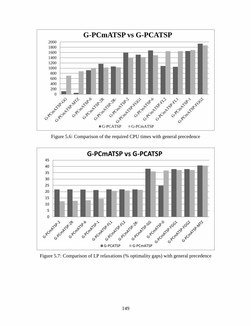
149

Figure 5.6: Comparison of the required CPU times with general precedence

Figure 5.7: Comparison of LP relaxations (% optimality gaps) with general precedence

0

200

400

600

800

1000

1200

1400

1600

1800

2000

G-PCmATSP vs G-PCATSP

G-PCATSP G-PCmATSP

0

5

10

15

20

25

30

35

40

45

G-PCmATSP vs G-PCATSP

G-PCATSP G-PCmATSP

150

5.7. Summary and concluding remarks

In this chapter, we have studied the performances of 26 different models for the mATSP

including transforming the mATSP to an equivalent ATSP formulation as proposed in [8, 140],

from the viewpoint of their relative tightness and effectiveness when directly solved using

CPLEX 12.1.0. These models are either new, exist in the current literature, or are modified

generalizations of existing ATSP models. The ATSP-MTZ, ATSP-KB, and ATSP-GG

formulations required the least CPU times for the set of problem instances utilized from the TSP

Library, and were more effective than their mATSP counterparts. For the remaining models, the

mATSP formulations outperformed the equivalent corresponding ATSP formulations. The

tightest LP relaxations for the non-precedence case were afforded by the following models:

{ATSP-6, ATSP-1, ATSP-2, mATSP-2R-, mATSP-2R, ATSP-FL1, ATSP-FL2, ATSP-2R

-,

mATSP-FL2, ATSP-2R, mATSP-2, mATSP-FL1, mATSP-1}. On the other hand, the mATSP-

MTZ and mATSP-KB formulations generally yielded weak LP relaxations, which could be a

critical issue for larger problem instances.

Furthermore, we considered mATSP problems in concert with two types of precedence

relationships. In the first case, the given precedence order between a pair of cities was enforced

only if both the cities were visited by the same salesman, designated PCmATSP. In the second

case, the specified precedence between any pair of cities was required to hold even if these cities

belonged to the tours of different salesmen, where the corresponding precedence was enforced

with respect to visit times as determined by the objective coefficient values, designated as G-

PCmATSP. The precedence-constrained versions of the mATSP-GG and mATSP-KB models

(denoted PCmATSP-GG and PCmATSP-KB) again required the least CPU times to solve our set

of test instances, in spite of enumerating a relatively larger number of branch-and-bound nodes.

The tightest LP relaxations were achieved by the flow-based models PCmATSP-6, PCmATSP-1,

PCmATSP-2R-, PCmATSP-2R, and PCmATSP-2. Additionally, the formulations that modeled

the PCmATSP directly, as opposed to transforming the problem into an equivalent ATSP

problem, were tighter and solved faster except for mATSP-0, thus making the PCmATSP

formulations preferable. For the generalized precedence case, the transformed ATSP-MTZ and

ATSP-GG formulations required the least CPU times by far followed by their mATSP

151

counterparts. Generally, the equivalently transformed ATSP formulations required less CPU

time, although this was not always the case. This variance in performance of different models in

the case of special precedence can be attributed to the ability of the mATSP formulations to

better differentiate among the tours of the m salesmen with reduced symmetry effects, thereby

leading to their superior performance. Interestingly, the direct modeling of the mATSP problem,

as opposed to equivalently transforming the problem to an ATSP, resulted in tighter

formulations. Overall, the mATSP formulations were tighter than the ATSP formulation for all

cases of precedence (namely, no precedence, special precedence, and general precedence). The

mATSP formulations consistently consumed smaller CPU times than their equivalent ATSP

counterparts for the case of special precedence. However, neither the mATSP models nor their

equivalent ATSP representations consistently outperformed the other for the no-precedence and

general precedence cases.

There appears to be a strong correlation between the size of the formulation and the required

CPU time. The simpler compact model formulations turned out to be preferable when solved

directly using CPLEX, although they possessed weaker LP relaxations. We believe that much of

this correlation is because of the relative ease of implementing branch-and-bound in a parallel

computing setting, where hundreds of thousands of nodes are visited during the process on eight

threads simultaneously, compared with the tight formulations that are often able to solve the

problem at the root node itself, but require a very long time to do so. The use of suitable

decomposition approaches coupled with advances in LP technology, might reverse this trend.

This is open to further investigation.

152

Chapter 6 Benders’ Decomposition for Problems with an Integer Sub-problem

6. Hidden figure

Table 6: Hidden table

6.1. Introduction

A Benders’ decomposition-based method is difficult to implement when the sub-problem is an

integer program. The difficulty arises because of the inability to obtain dual solution at an

integer solution point. In this chapter, we address this problem of generating a dual solution for

such a sub-problem. We present a general algorithm for this problem that determines it’s

optimal integer solution, and then, generate cuts at this solution point until the convex hull at that

point has been generated. With the knowledge of the polyhedron at that point, the LP solution

would give the necessary dual solution for generating a Benders cut for use in the Benders’

decomposition approach. In particular, we focus on such a decomposition scheme for the

multiple asymmetric traveling salesman problem (mATSP). In our decomposition scheme for

the mATSP, cities are allocated to tours in the master problem, and subsequently, the tour for

each salesman is determined in the sub-problem by solving m ATSPs. We, then, present an

application of this approach to a special case for which the convex hull at the integer point is

known. This special case belongs to the ATSP for which the DFJ cuts constitute the convex hull

of the problem [25]. The number of DFJ constraints grows exponentially with increase in the

number of cities in the problem, and hence, DFJ constraints are not typically used to solve a

problem. However, we only need a polynomial number of these constraints at a given integer

solution point. Therefore, we first find the optimal integer solution, and then, generate the DFJ

constraints that are tight at the optimal integer solution of the sub-problem.

In what follows, we first provide a literature review of several decomposition techniques. Then,

we prove validity of the proposed approach and apply it for the solution of the mATSP. To that

end, we present the model formulation for the mATSP. We also present results for our

numerical investigation on the use of the proposed approach. A significant cost is incurred to

implement this algorithm because of the number of integer problems that must be solved. We

also present techniques to speed up the computations with limited success.

153

6.2. Literature review on decomposition techniques

In this section, we provide an overview of three different decomposition techniques that have

been commonly used in the literature. These are: (1) column generation, (2) Lagrangian

relaxation, and finally, (3) Benders’ decomposition, which also includes logic-based Benders’

decomposition and Benders’ decomposition when encountering a mixed-integer-linear program

(MILP) in the sub-problem a relatively new method that shows a great potential.

6.2.1 Column generation

This decomposition method was first proposed by Dantzig and Wolfe [26], and it is often

referred to as the Dantzig-Wolfe decomposition method. When it is implemented for the

solution of a mixed linear programming problem, it is known as the branch-and-price method.

The general idea of column generation is to reformulate the problem by substituting the original

variables with a convex combination of the extreme points and a linear combination of the

extreme rays (when unbounded) of the polyhedron. This decomposition method divides the

problem into two or more problems. The first is known as the master problem while the

remaining problems are referred to as sub-problems. The goal of these problems is to break

apart the problem in such a way that the master problem can be used to determine the current

optimal dual multipliers that provide a lower bound (for minimization problems) while a sub-

problem is utilized as a pricing problem [32]. The process of solving the master problem

followed by a sub-problem is repeated until a stopping criterion is met, which typically pertains

to the optimality gap lying within an acceptable value, .

Column generation techniques have proven to be successful when the structure of a given

problem is known to have a block-diagonal or angular structure with complicating constraints.

The complicating constraints, sometimes referred to as coupling constraints, tie the problem

together requiring the solution of one large model. However, once these constraints are

removed, the remaining problem can be broken up into several smaller sub-problems that are

relatively easy to solve. (See [105] for an overview on decomposition techniques, and [29, 87]

for more details on column generation techniques.) Many problems naturally lend themselves to

the column generation method, which has been applied to problems in multi-commodity

154

network flows [6], lot sizing [13], scheduling [143], vehicle routing [76], cutting stock [9], and

airline and shipping industries [17, 80], to name a few.

The mATSP is very similar to a vehicle routing problem (VRP) in which each vehicle (salesman)

visits a subset of cities in the presence of constraints pertaining to total travel time, available time

windows, and/or vehicle capacity. A review of this problem containing model formulations of

its variations and methods used for its solution (column generation, Lagrangian relaxation, and

heuristics) can be found in [19]. For problems that model the transportation of vehicles, like

mATSP and VRP’s, column generation techniques are successful by first reformulating the

problem so that the master problem is a set partitioning formulation. This problem reformulation

allows each variable in the problem to represent a potential path or route to be taken by a single

salesman/vehicle. The main difficulty encountered when solving the master problem is that the

dual solution is needed for pricing each column. For this reason, the master problem must be

relaxed to be a linear problem. Once a solution to the master problem is obtained, the sub-

problem is solved to generate a column by optimizing the reduced cost.

In order to obtain a solution that is indeed feasible for the original integer problem, a branching

scheme on the original variables is employed. There are several methods to implement such a

scheme (see [19, 76]), and they are commonly referred to as “branch-and-price”. After

branching, the column generation method is re-implemented on each separable problem and the

process is continued until an optimal integer solution is found.

The sub-problem generates new routes for the master problem for inclusion as new variables,

and it can be formulated as an Elementary Shortest Path Problem (ESPP) or if given time

windows (TW) or capacity constraints (CC), it is formulated as an ESPPTWCC. The

ESPPTWCC is known to be NP-hard in the strong sense [35], and it is typically relaxed by

allowing cycles. This problem is identical for every salesman for the case of mATSP, and hence,

only needs to be solved once. However, it is separable for each salesman if dictated by an

application that the salesman are not identical. Specialized algorithms can be exploited for these

problems to speed up the solution time, namely, by using dynamic programming [30], to obtain

pseudo-polynomial computational time. This relaxation results in a slightly weakened lower-

155

bound with the advantage of much faster iterations in the sub-problem. Implementing 2-cycle

(or more) elimination results in tighter bounds [81]. Further work in dynamic programming in

this regard can be found in Chabrier [16] and Feillet [43].

For the mATSP, column generation is not suitable for many formulations since the problem is

reformulated as a set partitioning problem. With this in mind, we would like to exploit the

advantages of some newer formulations of mATSP due to the availability of tighter linear

relaxation formulations. It is our hope that these tighter formulations will lend themselves to

more successful decompositions.

6.2.2 Lagrangian relaxation

Lagrangian relaxation was initiated through the pricing ideas of Gilmore and Gomory’s column

generation by pricing in the simplex method [59, 60], and of course, Lagrange multipliers [39].

The idea of Lagrangian relaxation, in the context of this chapter, was first introduced by Held

and Karp [65, 66] for the traveling-salesman problem as described in [46], where the Lagrangian

vector plays the same role as Lagrange multipliers in constrained continuous optimization

problems [105]. The purpose of Lagrangian relaxation is to provide a good (tight) lower bound

on the objective function value. Typically, this is used in conjunction with a branch-and-bound

algorithm for the solution to combinatorial and/or integer problems.

Lagrangian relaxation is applied when the problem structure is the same as that for column

generation. Namely, the problem has a block diagonal structure and a set of complicating

constraints that, once removed, result in a much easier problem to solve. For Lagrangian

relaxation, these complicating constraints are removed from the constraint set, added to the

objective function, and are multiplied by a dual function [88]. Consequently the dual function

value is computed by solving a sub-problem and returning the dual values. The master problem,

with the relaxed constraints in the objective function, is then re-solved and the process is iterated

until a stopping criterion is met.

Lagrangian relaxation can be shown to be the same as column generation where the Lagrangian

relaxation is obtained by dualizing the complicating constraints from column generation [71]. It

156

is for this reason that often many problems that are effectively solved with column generation are

also effectively solved with Lagrangian relaxation. However, one drawback of Lagrangian

relaxation is that, in many types of problems like VRP and mATSP [19], it proves more difficult

to perform branching during a branch-and-bound algorithm. In [46], a list is provided of

problems for which Lagrangian relaxation has been applied. Some of these problems are: the

(asymmetric) traveling salesman problem, scheduling problems, general IP’s, location allocation

problems, generalized assignment problems, and set covering-partitioning problems (to include

the TSP reformulated as such).

Lagrangian relaxation has also been applied to the mATSP [56]. Its effectiveness results from

relaxing a part of the network flow constraints, which enables decomposition of the problem into

m problems, one for each tour. This problem potentially narrows the integrality gap between the

optimal solution of the linearized version of the problem as explained in [19] for the VRPTW

(see also [33]). Much recent work has been published in this area of VRPTWCC utilizing

Lagrangian relaxation in conjunction with column generation, and it is an area of active research.

6.2.3 Benders’ decomposition

In Benders’ decomposition [10], a series of master and sub-problems are solved iteratively,

similar to column generation. In fact, Benders’ decomposition can be viewed as the dual of

column generation, where the master problem of one is the sub-problem of the other. Note that,

in column generation, the initial problem is a restricted problem, since most or all the variables

are fixed to zero, and then, are allowed to be positive iteratively. While in Benders’

decomposition, the constraints are relaxed and iteratively added into the problem. Hence,

Benders’ decomposition is also known as a relaxation strategy. Benders’ decomposition works

most effectively on problems with a dual angular structure, similar to column generation, except

that instead of complicating constraints, in Benders’ decomposition, there is a set of

complicating variables. Geoffrion [57] has extended Benders’ decomposition for use on a

nonlinear convex problem.

In the master problem, the complicating variables are fixed to certain values, and then,

subsequently, the sub-problem is made relatively easier to solve. The sub-problem typically

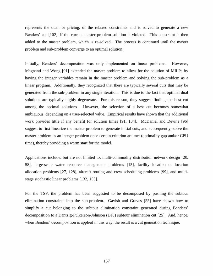
157

represents the dual, or pricing, of the relaxed constraints and is solved to generate a new

Benders’ cut [102], if the current master problem solution is violated. This constraint is then

added to the master problem, which is re-solved. The process is continued until the master

problem and sub-problem converge to an optimal solution.

Initially, Benders’ decomposition was only implemented on linear problems. However,

Magnanti and Wong [91] extended the master problem to allow for the solution of MILPs by

having the integer variables remain in the master problem and solving the sub-problem as a

linear program. Additionally, they recognized that there are typically several cuts that may be

generated from the sub-problem in any single iteration. This is due to the fact that optimal dual

solutions are typically highly degenerate. For this reason, they suggest finding the best cut

among the optimal solutions. However, the selection of a best cut becomes somewhat

ambiguous, depending on a user-selected value. Empirical results have shown that the additional

work provides little if any benefit for solution times [91, 134]. McDaniel and Devine [96]

suggest to first linearize the master problem to generate initial cuts, and subsequently, solve the

master problem as an integer problem once certain criterion are met (optimality gap and/or CPU

time), thereby providing a warm start for the model.

Applications include, but are not limited to, multi-commodity distribution network design [20,

58], large-scale water resource management problems [15], facility location or location

allocation problems [27, 128], aircraft routing and crew scheduling problems [99], and multi-

stage stochastic linear problems [132, 153].

For the TSP, the problem has been suggested to be decomposed by pushing the subtour

elimination constraints into the sub-problem. Gavish and Graves [55] have shown how to

simplify a cut belonging to the subtour elimination constraint generated during Benders’

decomposition to a Dantzig-Fulkerson-Johnson (DFJ) subtour elimination cut [25]. And, hence,

when Benders’ decomposition is applied in this way, the result is a cut generation technique.

158

Until recently, all known implementations of Benders’ decomposition have involved a linear

sub-problem. Next, we present three ideas that have been presented to solve the integer sub-

problem in Benders’ decomposition.

Hooker and Ottosson- Logic-based Benders’ decomposition [69].

In this paper, Benders’ decomposition is viewed as “learning from ones mistakes.” They

consider an inference dual which is a proof of optimality through use of logic where a proof

scheme is used to justify the inference dual. Many concepts and definitions exist for the dual in

a Benders’ decomposition context (see [69] for more detail). This work is typically applied

using constraint programming in the sub-problem [41, 68, 100]. However, for the context of the

mATSP, this technique does not seem promising.

Hamdouni, Desaulnier, and Soumis- Parking buses in a depot using block patterns [64].

Hamdouni et al. apply Benders’ decomposition with integer sub-problems through a branch-and-

bound type technique. First, they recognize that by relaxing the sub-problem to allow linear

solutions for the integer variables, the resulting solution provides a lower bound on the overall

problem. If the sub-problem, when relaxed, provides an integer solution, then the problem also

provides an upper-bound. With this knowledge, branching is applied in the master problem to

fathom most of the resulting branches during branch-and-bound method. Each branch is

exploited until the solution in the master problem is either fathomed as a result of poor bounds or

is completely fixed. For the latter, the sub-problem can be solved as an integer program since no

duals are required and the solution will be optimal for that given node.

They mention the possibility of branching in the sub-problem but state that this may “require

extensive computational effort because such decisions have a local impact on the model and

generally yield a very large search tree.” They further suggest that the cuts generated in the

ancestor nodes may not be tight.

159

Sherali and Fraticelli- A modification of Benders' decomposition algorithm for discrete sub-

problems [132].

The idea of using a cutting plane algorithm in the context of Benders’ decomposition with

integer sub-problems was first addressed by Fisher and Jaikumar [47] in a working paper

subsequently referenced by Federgruen and Zipkin [42]. However, the method was never

actually implemented in either paper.

Benders’ decomposition is used by Sherali and Fraticelli [132] to address a 2-stage stochastic

problem with integer recourse. The key issue is in providing dual multipliers to the master

problem from the sub-problem. In order to do this, the sub-problem is first relaxed to be linear

and then re-solved using lift-and-project techniques until the relaxed sub-problem generates

integer solutions. Cleary, the difficulty in this procedure is in the number of cuts needed to

generate integer solutions. Typically in a cutting plane algorithm, at some point, branching is

introduced due to the difficulty to make forward progress in the optimization process. Sherali

and Fraticelli suggest the implementation of RLT techniques (see [129-131]) to tighten the

model to limit the amount of cuts needed. For lifting the RLT constraints, they suggest

implementing the partial convexification cuts of Sherali et al. [133] and the lifting technique of

Balas et al. [5]. These constraints are generated in a way to ensure that they can be reused in the

next iteration of the sub-problem (by generating cuts for the non-decomposed problem and then

introducing them into the decomposed problem). Additionally, it is assumed that the master

problem is a pure integer problem. This assumption ensures that through branching in the master

problem the algorithm will terminate within a finite amount of time.

However, due to the difficulty of generating tight LP relaxations followed by a cutting plane

algorithm to find integer solutions with a linear model, this is expected to be too cumbersome to

effectively implement. Currently, the only known work to actually implement this technique is a

sequel paper by Sherali and Zhu [137]. In their work, a branch-and-bound technique is

implemented in the master problem, while a branch-and-cut technique is implemented in the sub-

problem to provide a tight enough linear relaxation of the convex hull to ensure integer solutions.

160

This process is carried out for a set of small problems where generating the necessary cuts in the

sub-problem was not an issue.

The algorithm that we suggest is similar in principle to Sherali and Fraticelli’s with the key

difference being that for our algorithm, we first find the integer solution for the sub-problem and

then generate the necessary cuts to define the convex hull at this point.

6.2.4 Combined decomposition techniques

Combinations of decomposition have proved successful in some applications. Cross

decomposition was first implemented by Van Roy [144, 145] as a mix of both Lagrangian

relaxation and Benders’ decomposition. Huisman et al. [71] combine column generation and

Lagrangian relaxation, as first suggested by Lobel [90] and Fischetti and Toth [45].

6.2.5 Acceleration techniques

For each of these decomposition techniques (column generation, Lagrangian relaxation, and

Benders’ decomposition), additional techniques may be applied to reduce the time to achieve an

optimal solution. It has been observed that the dual multipliers used typically have degeneracy

that can be removed by implementing a stabilization technique.

The generation of an initial solution as a warm start also proves helpful since much of the

instability occurs as a result of the initial duals used. And finally, for column generation and

Benders’ decomposition, it is a common practice to return multiple columns/cuts from the sub-

problem for the master problem. By providing multiple columns/cuts, the number of times that

the sub-problem must be solved can potentially be reduced.

6.3. Benders’ decomposition for integer sub-problems

For the general case integer sub-problem algorithm, when the convex hull is not known, after

solving the master problem in the usual way, we find the integer solution to the sub-problem and

then generate the convex hull of this solution. The algorithm then calculates the duals of the

integer solution to provide a valid Benders’ constraint. In this section, we present the details of

the general algorithm and prove its validity.

161

Currently, a common practice, for an integer sub-problem, is to solve the LP relaxation of the

integer problem. Once an optimal solution to the LP relaxation is found, the integer problem is

solved once as suggested by McDaniel and Devine [96]. Additionally, as discussed above,

Sherali and Fraticelli [132] suggest the use of a cutting plane algorithm to generate the convex

hull for the non-decomposed problem, and then, use these cuts in the sub-problem to tighten the

LP relaxation of the convex hull.

When the convex hull of an integer problem is used, the solution to the linear problem will

always result in an integer solution to the problem. The difficulty in implementing Benders’

decomposition directly on problems with integer sub-problems is the need of obtaining a dual

solution. By the solution method of Sherali and Fraticelli, the linear problem may be solved to

obtain the necessary dual variable values. However, typically, most cutting plane algorithms

need branching at some point in the algorithm because the gain from only using cuts often

deteriorates.

In light of the above, we propose the following scheme to obtain the dual solution for an integer

sub-problem. First, determine an optimal integer solution for the problem. Then, generate cuts

that pass through the corner point until the convex hull has been found (or sufficiently

approximated). Augment the sub-problem with these cuts and solve it as a linear program by

block pivoting to the optimal integer solution in one step. From this solution, we obtain the

necessary dual solution and generate a Benders’ cut to return to the master problem using

classical Benders’ decomposition techniques. Subsequently, verify the bounds and re-solve the

master problem are need be. This process is continued until an optimal solution is found and

verified. Figure 6.1 presents an overview of the algorithm.

In Propositions 1 and 2, below, we prove the validity of this algorithm by first showing that the

convex hull constraints about the optimal integer solution cut off the optimal LP solution. We,

then, show that the Benders’ cuts generated are valid cuts for the integer sub-problem.

162

Figure 6.1: Proposed algorithm to obtain dual solution for integer sub-problem

Proposition 1: When the optimal LP solution is not equivalent to the optimal integer solution,

the tight convex-hull-cuts at the optimal integer solution cut off the optimal LP solution.

Additionally, the new optimal LP solution occurs at the integer solution point.

Proof. We assume that there exists an optimal integer solution and an optimal LP solution that

are not the same. First, consider the feasible region between the optimal integer solution, the

optimal LP solution and the LP solution space that has a better objective function value than the

integer solution. (See Figure 6.2 for a graphical aid to this proof.) If the optimal LP solution is

to be cut off, then there must exist an integer solution within this described feasible region. If an

integer solution does not exist in this feasible region then, clearly, a convex hull constraint would

cut off the optimal LP solution. Now, assume that an integer solution does exist in this region,

thereby ensuring that the optimal LP solution is not cut off. However, this new integer solution

would have a better objective function value than the current optimal integer solution. This

163

violates our initial assumption of the location of the integer optimal solution. Hence, the convex

hull constraints about the optimal integer solution must cut off the optimal LP solution.

Additionally, we prove directly that the new optimal LP solution will be at the optimal integer

solution. After having generated the convex hull about the integer solution, a block pivot is

performed on the LP formulation to the optimal integer solution. Once at this point, pivoting

along any of the binding constraints will result in reaching another integer point (because the

convex hull has been generated about the optimal integer solution). And since the original point

is the optimal integer solution, all other adjacent integer points must have an equivalent or worse

objective function value. Hence, the optimal integer solution is also the optimal LP solution.

Figure 6.2: Graphical representation of the LP relaxation and convex hull

Proposition 2: The general case integer sub-problem Benders’ algorithm presented in this

section is a valid algorithm that converges to the globally optimal solution.

164

Proof. Proposition 1 proved that the optimal LP solution, prior to generating the convex hull

constraints, is cut off thereby resulting in the new optimal LP solution and the optimal integer

solution being the same. Hence, after generating the necessary constraints, a standard LP is

solved. From the LP we obtain the dual variable values and generate a Benders’ cut in the

normal way. This cut is then returned to the master problem. The Benders’ cut generated is a

classic Benders’ cut at an LP optimal solution (that happens to be integer as a result of utilizing

the convex hull). Therefore, this algorithm converges to the global optimal solution of the non-

decomposed problem by [10].

6.4. Benders’ decomposition for integer sub-problems-a special

case

A special case of the algorithm in Figure 6.1 occurs when the convex hull of the sub-problem is

known, but otherwise, is too expensive to directly implement. For such a problem, after finding

the optimal integer sub-problem solution, the convex hull constraints that are tight at the integer

solution are added to the problem and the problem is solved as an LP. Such a convex hull exists

for the ATSP, given by DFJ sub-tour elimination constraints [25], and can be used for the

solution to the mATSP. For the mATSP, we allocate the cities to tours in the master problem.

Consequently, the sub-problem pertains to solving m ATSPs. The so obtained m tours are

independent of one another, and hence, the solution to each tour can be obtained separately.

Once the integer solution has been found for an ATSP, we add the DFJ cuts that would be tight

at this point and solve the problem as a LP. The algorithm is continued by validating the

optimality gap between the master and sub-problems and then adding, as necessary, Benders’ cut

to the master problem using the duals corresponding to the optimal sub-problem integer

solutions.

Next, we describe generation of tight DFJ cuts at an optimal integer point of a sub-problem.

Given an integer solution to the ATSP, we need to generate all of the DFJ constraints that are

tight at that solution. The DFJ cuts for each tour are as follows:

,1,

SxSi ijSj

t

ijmtnSnVVS ,...,1 ,12},,...,1{, )(

(6.1)

165

where V is the set of all the cities in a sub-problem, S is every possible subset of the cities, and n

is the number of cities in the sub-problem. It has been shown that these constraints represent the

convex hull of the ATSP [63], these constraints grow exponentially with n. However, for a

given integer optimal solution, the only cuts that need to be generated are the ones that are tight

at that point. These constraints are generated by utilizing every subset VS such that all the

cities in S are visited sequentially on the tour that corresponds to the given integer solution. For

example, in the tour in Figure 6.3, the set { } will result in a tight DFJ constraint while

the set { } will result in a constraint that is not binding at the optimal integer solution

(we show this in Proposition 3). Given an ATSP with n cities, this will result in

constraints (shown in Proposition 4).

Figure 6.3: A graphical example of two sets that result in tight DFJ constraints

Proposition 3: Given an integer solution to the ATSP, the DFJ cuts generated using the

algorithm suggested are tight and represent the convex hull at this point.

Proof. We show that the DFJ constraints generated are tight when all the cities in S are visited

sequentially on the tour. Since all the cities in S are visited sequentially on the tour, the x-

variables representing this portion of the tour will be equal to one in the DFJ cut. Additionally,

there are 1S x-variables that are equal to one (this is easily verified via a counting argument),

and hence, the left hand side and right hand side of expression (6.1) are equal.

Next, we prove that there are no other constraints that are tight for the DFJ cuts. Assume that

there is a set S that has at least one city that is not directly visited by any other city in S. For

166

every two cities in the set that are sequential, there will be one x-variable that is equal to one.

However, since at least one city in S cannot be directly sequenced, no more than 2S x-

variables will be equal to one, and hence the DFJ cut will not be tight. Since all the tight

(binding) constraints have been generated for a given integer solution, by the generated DFJ

constraints represent the convex hull at the optimal integer solution [63].

Proposition 4: There are DFJ constraints generated that are tight for any integer

solution for the ATSP.

Proof. By Proposition 3, the only tight DFJ constraints are generated by the algorithm. There

are potential sizes for the cardinality of S for | | . Each size of the

set S has a total of n different constraints that can be generated by the algorithm, one for each

starting location of the sequential path on the tour. Hence, DFJ constraints are

generated.

The advantage to solving the integer sub-problem by utilizing the proposed algorithm is that the

mATSP need not be solved directly. The mATSP tends to be expensive to formulate, is

generally slow to solve, and it requires a significant amount of RAM. By utilizing Benders’

decomposition, rather than solving the problem directly, several smaller problems are solved.

This potentially allows for the solution of larger problems. However, the potential disadvantage

of the proposed algorithm is that the smaller problems must be solved several times. After

decomposition, first one allocation master problem is solved for allocating n cities to the m tours.

Consequently, m ATSPs are solved and the bounds are verified. Hence, in each iteration, m+1

integer formulations are solved. In the subsequent section, we provide an empirical analysis of

two different model formulations for mATSP that are solved directly via CPLEX 12.1.0 and by

utilizing the proposed algorithm.

6.5. Model presentation, empirical investigation, and results

In this section, first we present two model formulations for the mATSP. We also present the

master problem and sub-problem formulations of Benders’ decomposition for the

implementation of the proposed algorithm. We utilize CPLEX 12.1.0 to find solutions of the

167

master and sub-problems. This is followed by the presentation of results of an empirical

investigation conducted to study the performance of direct solution of the model formulation of

the mATSP using CPLEX 12.1.0 and solution using the proposed algorithm when applied to a

mix of problems from the TSP library [1] and a set of randomly generated data. The random

problems were generated using Euclidean distances between cities. For each test case, the

number of salesmen (m) was varied. The computations were performed using CPLEX 12.1.0

with OPL 6.3 on an Intel Xeon E5335 2.00 GHz computer with 3 GB of RAM and running

Windows VISTA.

6.5.1 MTZ non-decomposed model

The first of these formulations is a lifted version of the Miller-Tucker-Zemlin (MTZ) [101]

formulation. It is a relatively simple formulation that is quick to solve. The drawback of this

formulation is the looseness of the LP relaxation. A previous study has found the average

optimality gap of the LP relaxation to be 30.30% with an average solution time of 0.67 seconds

[121] (see Chapter 5). The second formulation is a generalization of the multi-commodity flow

model proposed for the ATSP in [150]. The strength of this formulation is in the tightness of its

LP relaxation. As represented in [121], the average optimality gap of the LP relaxation of this

formulation is 0.28%. However, this tight LP formulation comes at the cost of a model that is

harder to solve, where the average LP relaxation solution time was found to be 173.42 seconds.

Most of the formulations based on the ranking of cities [18, 54, 77, 140] have extended the MTZ

formulation for the single asymmetric traveling salesman problem to the m-salesman case

(designated as mATSP-MTZ). To present such an extension, we define the decision variables:

,0

,1t

ijx if city i directly precedes city j on the tour by salesman t

otherwise, ,...,mj,t,...,n,ii,j 11

t

iu a rank order index associated with city i, ,,...,2 ni mt ,...,1

Without loss of generality, we assume city 1 to be the base city and accordingly set and

we let where denotes the maximum number

of cities from { } that can be visited by any salesman. This yields the following basic

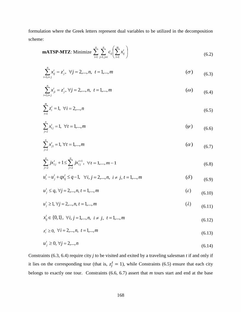
168

formulation where the Greek letters represent dual variables to be utilized in the decomposition

scheme:

mATSP-MTZ: Minimize

n

i

n

ijj

m

t

t

ijij xc1 ,1 1

(6.2)

,,1

t

j

n

jii

t

ij zx

,,...,2 nj mt ,...,1 )(

(6.3)

,,1

t

j

n

jii

t

ji zx

,,...,2 nj mt ,...,1 )(

(6.4)

,11

m

t

t

iz ni ,...,2

(6.5)

,12

1

n

j

t

jx mt ,...,1 )(

(6.6)

,12

1

n

j

t

jx mt ,...,1 )(

(6.7)

,12

1

1

2

1

n

j

t

j

n

j

t

j jxjx 1,...,1 mt

(6.8)

,1 qqxuu t

ij

t

j

t

i ,,...,2, nji ,ji mt ,...,1 )(

(6.9)

,qu t

j ,,...,2 nj mt ,...,1 )(

(6.10)

,1t

ju ,,...,2 nj mt ,...,1 )(

(6.11)

},1 ,0{t

ijx

,,...,1, nji ,ji mt ,...,1

(6.12)

,0t

iz ,,...,2 ni mt ,...,1

(6.13)

,0t

ju nj ,...,2

(6.14)

Constraints (6.3, 6.4) require city j to be visited and exited by a traveling salesman t if and only if

it lies on the corresponding tour (that is, ), while Constraints (6.5) ensure that each city

belongs to exactly one tour. Constraints (6.6, 6.7) assert that m tours start and end at the base

169

city. Constraints (6.8) impose hierarchical restrictions in the spirit of Sherali and Smith [136] to

defeat symmetry among the salesmen. Constraints (6.9-6.11) enforce the well-known Miller-

Tucker-Zemlin (MTZ) subtour elimination constraints (SECs), and Constraints (6.12-6.14)

represents the logical restrictions on the decision variables.

6.5.2 FL2 non-decomposed model

Our second model is based on a multi-commodity flow model. Laporte and Norbert [86] have

extended the ATSP formulation of Dantzig-Fulkerson-Johnson (DFJ) [25] to the m-salesman

case, and have adopted a LP-based relaxation approach that imposes subtour elimination and

integrality restrictions when needed. Wong [150] established the equivalence of a polynomial

length maximum flow-based formulation for ATSP to the exponentially-sized formulation based

on the DFJ subtour elimination constraints. This equivalence holds for the m-salesman versions

of these respective formulations as well. Below, we provide a model (mATSP-FL2) for mATSP

that is a generalization of the model proposed for ATSP in [150] that was initially proposed by

Sarin et al. [121] (See also Chapter 5). Due to the presence of m salesmen, we also include

certain symmetry breaking constraints. Consider the following set of decision variables, in

addition to the (x, z)-variables defined above:

tv

ijp )(

1, if flow occurs on arc (i, j) for the vth

commodity sent from the base city 1 to

city v via the tour of salesman t

0, otherwise, .,...,1,,...,2,,,...,1, mtnvjinji

The flow-based formulation for the mATSP, referred to as mATSP-FL2, can be stated as

follows:

mATSP-FL2: Minimize

n

i

n

ijj

m

t

t

ijij xc1 ,1 1

(6.15)

subject to

,,1

t

j

n

jii

t

ij zx

,,...,2 nj mt ,...,1 )(

(6.16)

,,1

t

j

n

jii

t

ji zx

,,...,2 nj mt ,...,1 )(

(6.17)

170

,11

m

t

t

iz ni ,...,2

(6.18)

,12

1

n

j

t

jx mt ,...,1 )(

(6.19)

,12

1

n

j

t

jx mt ,...,1 )(

(6.20)

,12

1

1

2

1

n

j

t

j

n

j

t

j jxjx 1,...,1 mt

(6.21)

,)( t

ij

tv

ij xp ,,...,1, nji ,ji ,,...,2 nv mt ,...,1

(6.22)

,)( 11

,2

t

v

t

v

tv

j

n

vjj

zxp

,,...,2 nv mt ,...,1 )(

(6.23)

,0)()(,,1,,2

tv

ji

n

vijj

t

iv

tv

ij

n

vijj

pxp ,,...,2, nvi ,vi .,...,1 mt

(6.24)

},1 ,0{t

ijx ,,...,1, nji ,ji mt ,...,1

(6.25)

,0t

iz ,,...,2 ni mt ,...,1

(6.26)

,0)( tv

ijp

,,...,1, nji ,ji ,n,...,v 2 ,,...,1 mt with

,0)( 1 tv

jp ,,...,2 nj ,,...,2 nv ,jv ;,...,1 mt and

,0)( tv

vjp ,,...,1 nj ,,...,2 nv ,jv .,...,1 mt

(6.27)

Constraints (6.16-6.21) are identical to Constraints (6.3-6.8) in mATSP-MTZ. Constraints (6.22-

5.34) are used to model multi-commodity flows, each related to . In particular, for

each salesman, Constraint (6.22) allows flow to occur from city i to city j only if , and

Constraints (6.23, 6.24) constitute flow-balance restrictions. Constraints (6.25-6.27) impose

logical restrictions on the decision variables, where again, the integrality of the (z, p)-variables

follows from the remaining model constraints.

6.5.3 Proposed algorithm for MTZ and FL2

Next, we present model formulations for the proposed Benders’ decomposition method involving

integer sub-problem. In the master problem, the cities are allocated to tours, while in the sub-

171

problem m ATSPs are solved. The formulation for the master problem is the same for both the

mATSP-MTZ and mATSP-FL2 models. We introduce a new variable, ,objz to represent the

objective function of the master problem. Benders’ cuts are iteratively added to the problem,

increasing the value of ,objz until an optimal solution is found and verified.

mATSP-MP: Minimize objz

(6.28)

Subject to:

,11

m

t

t

iz ni ,...,2

(6.29)

,12

n

i

t

iz mt ,...,1

(6.30)

,22

1

n

j

t

i

n

j

t

i jzjz mt ,...,2

(6.31)

},1,0{t

iz ni ,...,2

(6.32)

0objz

(6.33)

Constraints (6.29) are the same as Constraints (6.5) that ensure that every city is allocated to a

tour. Constraints (6.30) enforce each tour to have at least one city to visit. Constraints (6.31)

provide symmetry breaking constraints among the several tours, while Constraints (6.32, 6.33)

provide logical restrictions on the variables.

Once the master problem has been solved to optimality for the integer problem, the solution is

provided as an input for the sub-problem. The sub-problem formulations for mATSP-MTZ and

mATSP-FL2 are identical to their original formulations after dropping Constraints (6.5, 6.8) and

(6.18, 6.21), respectively, from the formulations and treating the z-variables as constants in the

formulations. Additionally, we point out that the m tours can be solved independently.

After the solution of each ATSP, the DFJ Constraints (6.1) that are tight at the integer solution

are added to the formulation, and the LP relaxation is solved as described above via a block pivot

to the optimal integer solution. The duals at the optimal solution are generated and the following

Benders’ cut is added to their respective master problems:

172

m

t DFJk

t

k

t

k

MTZ

objt

Sz1

)1(

m

t

n

j

t

j

t

j

t

j

n

j

t

j

t

j

n

i

n

jij

t

ij

tt zqq1 222 ,2

)1(

(6.34)

m

t DFJk

t

k

t

k

FL

objt

Sz1

2 )1( ,1 2

m

t

n

j

t

j

t

j

t

j

t

j

tt z

(6.35)

where DFJt is the set of constraints that were generated from the DFJ algorithm on tour t and

t

kS

is the number of cities utilized for each DFJ constraint k generated on tour t. After every

iteration, the optimality gap between the master problem objective function and the best sub-

problem objective function is compared. This process is continued until the optimality gap is

less than some predefined tolerance.

In order to speed up the algorithm, the warm start technique of McDaniel and Devine [96] is

implemented. For this implementation, the master and sub-problems are both solved in their

linear relaxed form (we call this warm start Phase 1 or W1). Once the linear formulation

converges, we then solve the master problem as an integer problem while still solving the sub-

problem using the linear relaxation (we call this warm start Phase 2 or W2). Once this

formulation converges, the proposed method is implemented (called Phase 3 or just simply 3).

Solving the problem in this way helps in obtaining a good starting solution. We implemented

this method along with directly solving the problem using the proposed algorithm (that is, simply

Phase 3).

6.5.4 Empirical investigation and results

The results for the problems from the TSP library and for the randomly generated data are

displayed in Tables 6.1 and 6.2, respectively, where “m” is the number of salesmen, “Model” is

the model formulation, “Int. CPU” is the time to solve the non-decomposed integer problem to

optimality, and LP lower bound is the non-decomposed LP lower bound. Both the direct

solution methodology and the proposed algorithm were run either until an optimal solution is

proved or a time limit of 3600 seconds (1 hour) is reached. The LP phase is the same as

173

presented above where W1 and W2 is presented in the column labeled LP phase whenever the

model stopped before reaching an optimal solution, as a result of reaching the 3600 second time

limit while in warm start Phase 1 and 2, respectively. (Recall that W1 = LP master and sub-

problem, W2 = Integer master and LP sub-problem, 3 = Integer master and sub-problem.) For

every dataset and model, the algorithm was first ran with the warm start and then again without

the warm start. (This is clearly seen by looking at the number of LP iterations column.) We

emphasize for the reader that the upper bound presented is the current phase (W1, W2, 3) upper

bound. Hence, if at 3600 seconds of CPU time, the algorithm was in W2, then the upper bound

represents the upper bound on the LP solution, not the integer solution. Both W1 and W2 were

run until within 5% of their respective optimal solutions, and then, the next phase was started,

where the lower bound remained the same and the upper bound was reset to positive infinity.

The remaining columns are used to track the number of iterations and time spent in the master

problem (MP), sub-problem (SP), and for solving the LP and integer problems.

Unfortunately, for every case tested, the direct solution method is much faster than solving the

problems via decomposition. We believe that this is caused from the sheer number of problems

that are solved in the algorithm, where m+1 problems are solved in each iteration. Although

each of these problems is smaller than the non-decomposed problem, this benefit does not seem

to outweigh the cost of re-solving each smaller model several times. The cause of having to run

so many iterations stems from the fact that initially the master problem has no information about

the structure of the sub-problems. With each iteration of the algorithm, the master problem

gathers more information about the problem structure until an optimal solution is achieved.

The MTZ linear problem was generally faster to use, resulting in a large amount of information

for the master problem without using a significant amount of CPU time. However, the MTZ

linear problem is very loose, resulting in poor bounds on the integer problem. Conversely, the

FL2 linear problem is expensive, but has very tight bounds. In every instance where Phase 3 was

reached after the warm start, the first integer solution found was also the optimal solution. This

fact makes the tight FL2 models attractive to use. In Phase W2 and Phase 3 of the algorithm,

generally, the tour allocation of the sub-problem was the most difficult part of the algorithm. For

174

both models, the warm start improved the effectiveness of the algorithm, decreasing the required

CPU times when an optimal solution was found, and tightening the bounds.

Table 6.1: Empirical investigation using the mATSP data

Dataset m Int.

Sol'n Model Int. CPU

LP lower bound

LP phase

No. of LP iterations

No. of Int. iterations

Lower and upper bound

Opt % Gap

Total CPU

MP CPU

SP CPU

Total LP CPU

Total Int. CPU

br17 2 39.00 MTZ 0.40 8.13 3 263 1017 34-42 19.05 3600.00 2024.78 687.1 3.60 3592.13

3 0 1099 33-42 21.43 3600.00 2236.21 591.89 0 3600.00

FL2 5.76 39.00 3 97 1 39-39 0.00 71.11 4.82 59.59 68.30 2.86

3 0 504 23-45 48.89 3600.00 877.36 1300.06 0 3600.00

3 42.00 MTZ 0.22 14.29 3 478 336 16-45 64.44 3600.00 2874.88 378.37 108.50 3502.27

3 0 602 2-186.00 98.28 3600.00 3322.72 338.56 0 3600.00

FL2 7.29 42.00 3 462 1 42-42 0.00 1307.09 165.20 935.01 1295.05 12.28

3 0 340 0-52 100.00 3600.00 367.42 1712.53 0 3600.00

4 47.00 MTZ 0.14 20.46 W2 1031 38 19.85-22 9.78 3600.00 2409.40 1012.72 1349.25 2298.33

3 0 647 0-61 100.00 3600.00 2211.46 701.35 0 3600.00

FL2 4.42 47.00 W1 501 0 0-71.98 100.00 3600.00 578.80 3079.31 3600.00 0

3 0 254 0-61 100.00 3600.00 306.65 1767.90 0 3600.00

ftv33 2 1302 MTZ 0.42 1211.10 3 302 164 1209-1302 7.14 3600.00 3203.04 217.75 98.31 3482.71

3 0 214 555-1433 61.27 3600.00 3361.63 86.20 0 3600.00

FL2 37.94 1302.00 W1 139 0 1125.4-1461.16 22.98 3600.00 758.95 2621.21 3600.00 0

3 0 72 516.5-1433 63.96 3600.00 480.21 1295.25 0 3600.00

3 1328 MTZ 0.44 1238.00 W2 1023 0 1229-1258.06 2.31 3600.00 2435.12 1164.33 3600.00 0

3 0 305 0-1693 100.00 3600.00 3102.60 228.51 0 3600.00

FL2 180.76 1328.00 W1 95 0 538.03-1858.87 71.06 3600.00 638.59 3075.04 3600.00 0

3 0 48 0-1693 100.00 3600.00 429.92 1435.94 0 3600.00

4 1367 MTZ 0.53 1266.10 W1 1076 0 1168.02-1328.65 12.09 3600.00 608.59 2334.50 3600.00 0

3 0 602 0-1952 100.00 3600.00 426.09 1405.01 0 3600.00

FL2 253.47 1367.00 W1 71 0 0-2066.55 100.00 3600.00 519.05 3083.25 3600.00 0

3 0 36 0-1952 100.00 3600.00 288.14 1835.53 0 3600.00

ftv35 2 1489 MTZ 1.42 1395.40 3 334 179 1396-1483 5.87 3600.00 3046.71 348.60 130.11 3474.25

3 0 156 569.6-1601 64.42 3600.00 3466.08 61.41 0 3600.00

FL2 102.37 1466.50 W1 118 0 1219.21-1586.6 23.16 3600.00 807.33 2743.79 3600.00 0

3 0 60 564-1601.5 64.78 3600.00 731.51 1498.01 0 3600.00

3 1511 MTZ 0.90 1422.00 W2 1155 0 1419-1436.23 1.20 3600.00 2162.21 1483.23 2769.15 830.85

3 0 288 0-1776 100.00 3600.00 3103.82 224.97 0 3600.00

FL2 3600.00 1495.50 W1 79 0 513.65-2062.67 75.09 3600.00 772.43 2827.83 3600.00 0

3 0 41 0-1776 100.00 3600.00 476.85 1603.54 0 3600.00

4 1551 MTZ 0.76 1464.10 W1 1040 0 1342.57-1556.35 13.74 3600.00 607.49 2329.46 3600.00 0

3 0 584 0-2202.31 100.00 3600.00 402.25 1413.84 0 3600.00

FL2 1625.20 1539.50 W1 60 0 0-2481.06 100.00 3600.00 472.31 3127.69 3600.00 0

3 0 30 0-2205 100.00 3600.00 404.13 1393.96 0 3600.00

5 1595 MTZ 1.63 1511.96 W1 863 0 1246.55-1664.37 25.10 3600.00 535.43 2472.41 3600.00 0

3 0 481 0-2248 100.00 3600.00 314.52 1475.93 0 3600.00

FL2 3521.01 1584.50 W1 48 0 0-2158.2 100.00 3600.00 363.44 3236.56 3600.00 0

3 0 24 0-2248 100.00 3600.00 211.15 1261.74 0 3600.00

175

Table 6.2: Empirical investigation using random data

Dataset m Int.

Sol'n Model

Int. CPU

LP lower bound

LP phase

No. of LP iterations

No. of Int. iterations

Lower and upper bound

Opt % Gap

Total CPU

MP CPU

SP CPU

Total LP CPU

Total Int. CPU

Rand10 2 1.68 MTZ 0.08 1.13 3 46 34 1.68-1.68 0.00 4.63 0.90 1.83 0.80 3.85

3 0 59 1.68-1.68 0.00 4.79 0.83 1.87 0 4.79

FL2 0.04 1.68 3 37 1 1.68-1.68 0.00 2.65 0.33 1.95 2.40 0.25

3 0 47 1.68-1.68 0.00 8.47 0.99 3.33 0 8.49

3 2.18 MTZ 0.07 1.65 3 104 42 2.18-2.18 0.00 22.06 6.43 9.08 5.12 16.94

3 0 127 2.18-2.18 0.00 42.67 17.20 11.16 0 42.68

FL2 0.06 2.18 3 124 1 2.18-2.18 0.00 28.55 3.91 20.41 27.33 1.25

3 0 160 2.18-2.18 0.00 166.46 44.26 54.20 0 166.52

4 3.03 MTZ 0.18 2.52 3 123 68 3.03-3.03 0.00 89.53 42.68 25.90 13.09 76.47

3 0 302 3.03-3.03 0.00 519.97 301.27 99.06 0 520.01

FL2 0.09 3.03 3 230 1 3.03-3.03 0.00 140.58 17.87 103.07 137.18 3.46

3 0 366 3.03-3.03 0.00 1489.07 500.45 450.99 0 1489.19

Rand20 2 0.91 MTZ 0.42 0.65 3 164 658 0.74-0.91 18.68 3600.00 2761.96 413.08 14.25 3581.78

3 0 465 0.14-1.23 88.62 3600.00 3267.07 157.86 0 3600.00

FL2 4.08 0.91 3 228 1 0.91-0.91 0.00 367.35 40.57 276.13 361.26 6.21

3 0 329 0-1.41 100.00 3600.00 542.06 1367.68 0 3600.00

3 0.92 MTZ 0.44 0.65 3 825 247 0.64-0.98 34.33 3600.00 2373.11 718.39 600.21 3018.88

3 0 1046 0-1.71 100.00 3600.00 509.89 1330.92 0 3600.00

FL2 14.23 0.92 W1 437 0 0-2.07 100.00 3600.00 618.17 2791.73 3600.00 0

3 0 219 0-1.72 100.00 3600.00 412.50 1611.75 0 3600.00

4 0.93 MTZ 0.34 0.66 W2 1399 4 0.65-0.74 12.61 3600.00 1003.17 2094.87 3150.86 527.2

3 0 835 0-2.06 100.00 3600.00 392.30 1416.56 0.00 3600.00

FL2 13.03 0.93 W1 334 0 0-2.68 100.00 3600.00 502.22 2838.32 3600.00 0

3 0 162 0-2.56 100.00 3600.00 319.99 1496.01 0.00 3600.00

Rand30 2 0.86 MTZ 0.26 0.60 3 394 164 0.59-1.09 45.92 3600.00 2334.46 1080.98 125.12 3465.49

3 0 750 0-1.27 100.00 3600.00 1778.30 1032.30 0 3600.00

FL2 28.85 0.86 W1 199 0 0.36-1.29 71.81 3600.00 601.81 2621.15 3600.00 0

3 0 102 0-1.31 100.00 3600.00 849.88 1664.93 0 3600.00

3 0.94 MTZ 3.06 0.67 W2 1370 1 0.65-0.71 9.39 3600.00 804.70 1820.33 3399.52 200.00

3 0 815 0-1.83 100.00 3600.00 432.31 1299.98 0 3600.00

FL2 118.25 0.94 W1 136 0 0-2.29 100.00 3600.00 527.91 2727.40 3600.00 0

3 0 69 0-1.95 100.00 3600.00 351.79 1518.90 0 3600.00

4 1.04 MTZ 1.79 0.78 W1 1107 0 0.54-0.84 35.89 3600.00 482.5 2083.96 3600.00 0

3 0 642 0-2.45 100.00 3600.00 331.25 1399.87 0 3600.00

FL2 1183.30 1.03 W1 99 0 0-3.04 100.00 3600.00 520.28 2741.79 3600.00 0

3 0 51 0-2.92 100.00 3600.00 356.34 2080.50 0 3600.00

To study the tail behavior of the algorithms, we ran the FTV 35 m = 2 data set for 24 hours. The

upper and lower bounds for each run are shown in Figure 6.4. These runs were made using a

much faster Intel Core i7 CPU 870 2.93 quad core computer with 8 GB of RAM and running

Windows 7. First, we note that the MTZ linear problem upper bound is non-monotonic as a

result of the algorithm transitioning between phases. (The upper bound is reset at the beginning

of each new phase.) All the other runs of the algorithm remained in the same phase that they

started in (W1 or 3). With the exception of the MTZ linear problem run, the optimality gap is

converging slowly, as can be seen in Figure 6.4. However, for the MTZ linear problem run, the

176

gap appears to be converging to the optimal solution. The MTZ linear problem run resulted in

the tightest gap, and appears to be the most likely run to first converge to the optimal solution.

Table 6.3 displays the total number of linear problems and integer iterations performed, the

lower and upper bounds, and the optimality gap after 24 hours for these runs.

Additionally, we ran the formulations on a 45 city set of random data but have not presented the

results in the table because none of the models had improved their bounds after the 3600 second

time limit except for the MTZ model with the warm start implementation. For this model, the

optimality gap achieved was 5.02% in warm start Phase 2.

Figure 6.4: Upper and lower bounds for the ftv35 m = 2 data set

W2 starts and ends here, started Phase 3

177

Table 6.3: No. of iterations, bounds, and optimality gap for the ftv35 m = 2, 24 hour run

Model No. of LP

iterations

No. of Int.

iterations

Lower

bound

Upper

bound

Optimality

gap

MTZ 334 5 1393.00 1486.00 6.26

0 34 302.00 1601.00 81.14

FL2 313 0 1418.62 1540.62 7.92

0 37 494.00 1610.00 69.00

Finally, the code developed for the implementation of the algorithms was rudimentary, did not

exploit the use of parallel processors as done by CPLEX. Hence, some minor gains could be

further achieved by removing some of the delays while transforming the data and establishing

the next iteration’s input data.

The proposed algorithm will further be slower in case the convex hull is not known a priori, and

therefore, will have to be generated. To help speed this process, the cuts utilized by CPLEX

when solving the integer sub-problem could be exploited. Additionally, the algorithm could be

implemented to exploit the structure of the MTZ and FL2 models, where the MTZ model is used

to find the integer solutions (since it is faster), and then, the FL2 model is used to generate the

duals to provide a tighter feasible region with tighter dual solutions.

6.6. Concluding remarks In this chapter, we have presented a method of using Benders’ decomposition when the sub-

problem is an integer program. We have applied it to solve the mATSP for which the sub-

problem is an ATSP. Since the DFJ subtour elimination constraints constitute the convex hull

for ATSP, we were able to effectively obtain dual solution of the integer sub-problem in order to

generate a Benders’ cut for inclusion in the master problem. This method, while theoretically

valid and stimulating, resulted in computation times that were far from superior when compared

with those obtained by solving a model formulation of mATSP directly using CPLEX.

Additionally, as the problem size increases, the effectiveness of the proposed methods

deteriorates further because of a greater effort required in solving a more complex master

problem.

178

Chapter 7 Concluding Remarks and Directions for Future Research

7. Hidden figure

Table 7: Hidden table

In this dissertation, we have addressed the modeling and analysis of a biomass logistics system.

We have presented the various problems involved in the design of such a system in Chapter 1.

The key decisions involved are: locations of satellite storage locations (SSLs), allocation of

production fields to SSLs, allocation of SSLs to bio-crude plants (BcP), locations of BcPs, and

the routing of equipment sets among the SSLs for their unloading to transport biomass to BcPs.

The routing of equipment sets among the SSLs also constitutes a multiple traveling salesman

(mATSP) type of problem. In Chapter 2, we have provided a detailed description of a feedstock

logistics system in order to highlight its key features, and also, presented an accurate set of

parameters for use in the model formulations of the feedstock logistics problems. To this end,

we described the need for contract agreements to address the long-term risks of the production

field owner and the owner of a bio-crude plant BcP. The manner in which the harvesting

equipment is used can impact its utilization and operating cost. We presented two systems for

the ownership of the equipment: active and passive ownership. For active ownership, the

harvesting equipment is owned by the field owner. This system results in a significantly higher

equipment cost because of the lack of equipment utilization. For the passive system, the field

owner uses a custom harvest company to own and operate the equipment for the harvesting and

storage of biomass. This leads to issues pertaining to field management and harvest windows,

which may be constrained by requirements specified by the BcP owner as well as by the weather.

We, then, established three equipment options for the unloading of biomass at a SSL. The three

systems, namely, rear-loading rack, side-loading rack, and densification options, were described

in detail along with their respective costs. This was followed by an example scenario for a single

and fixed BcP. This preliminary analysis was conducted to provide an intuition for the results

obtained from the cost figures that were established.

In Chapter 3, we have analyzed a feedstock logistics problem when the location of the BcP is

known a priori. We developed a mathematical model for this problem and used it to study the

effect of using various options at the SSLs. In particular, we studied the performances of the

179

three equipment options that were presented in Chapter 2. The data that we used for this

investigation pertained to a real-life scenario in Gretna Va. Our results show that the side-

loading rack system encountered the least total cost. This optimal solution obtained by using our

model was compared with that obtained using the heuristic method proposed in the literature,

and it shows the extent of benefit achieved through the use of a mathematical formulation

method in order to reduce the overall system cost. Finally, we performed a sensitivity analysis on

the input parameters that revealed the most significant problem features for reducing the total

cost, which constitute transportation of biomass from the product fields to the SSLs, the grinding

operation, and the biomass yield.

In Chapter 4, we extended the problem addressed in Chapter 3 to determine the locations of

several BcPs in order to serve a refinery. We also proposed a nested Benders’ decomposition-

based methodology for the solution of the problem. To the best of our knowledge, this nested

Benders’ decomposition-based methodology has been developed for the first time for the

deterministic problems. We proved the validity of this nested Benders’ decomposition-based

methodology. We also tested the effectiveness of this methodology by applying it to a real-life-

based data set for locating 5 BcPs in Virginia and North Carolina. Our results demonstrate the

efficacy of using this methodology on larger-sized instances over the direct solution of its model

formulation by CPLEX 12.1.0.

In Chapter 5, we have presented an analysis of 13 formulations for the mATSP and, additionally,

a mapping of these 13 formulations to their equivalent ATSP formulations. These formulations

are either new or those presented in the literature. The strength and weaknesses of these 26

formulations were compared using a computational investigation. Additional special and general

precedence relationships among cities and tours were then established, modeled, and analyzed.

These results have revealed that the formulations based on the rankings of cities requires the

smallest CPU times, but also, they have the loosest LP relaxations. Conversely, the multi-

commodity flow models have extremely tight LP relaxations, but were slow at finding and

proving optimality.

180

In the final chapter, we have proposed a method for applying Benders decomposition when the

sub-problem is an integer program. For these problems, the only known, general technique to

find proper Benders’ cuts is to use a cutting plane algorithm in the sub-problem until the integer

solutions are generated. However, cutting plane algorithms by themselves tend to be slow. For

our methodology, we first obtain an integer optimal solution of the sub-problem, and then,

generate the needed constraints that define the convex hull about the optimal integer solution.

We demonstrate this methodology for the solution of the mATSP because the sub-problem

obtained as a result of decomposition is an ATSP for which the convex hull is known and can be

used to obtain the dual solution at an integer optimal solution. This method guarantees

convergence to the global optimal solution. However, our computational investigation

demonstrated that this method is slow compared with direct solution of model formulation

obtained using CPLEX 12.1.0. This is mainly because of the large number of integer models

that must be solved at each iteration.

In this dissertation, we have addressed a feedstock logistics system that covers decisions

involved from the production field to a refinery. Our research has contributed to a better

understanding of the overarching problems and solution of a feedstock logistics problem. For

future research, we suggest a study of the inventory risk problem associated with the

management of the baled biomass. Coupled with this problem, is the issue of scheduling the

harvesting operations. The need for continual flow of biomass into a BcP plant, weather

limitations (because of harvesting window), and inventory management make the scheduling of

the harvesting operations a non-trivial task. Finally, we suggest expansion of our model to

include two additional features: (1) location of several small refineries over a region, and (2)

distribution in a cost-effective manner of refined oil from the refineries for consumption by

consumers.

181

References . [1] (15 May). TSPLIB- Library of traveling salesman problems. Available:

<http://www.iwr.uni-heidelberg.de/groups/comopt/index.html>

[2] P. Appelqvist and J. M. Lehtonen, "Combining optimisation and simulation for steel

production scheduling," Journal of Manufacturing Technology Management, vol. 16, pp.

197-210, 2005.

[3] T. W. Archibald, C. Buchanan, K. McKinnon, and L. Thomas, "Nested Benders

decomposition and dynamic programming for reservoir optimisation," Journal of the

Operational Research Society, pp. 468-479, 1999.

[4] N. Ayoub, R. Martins, K. Wang, H. Seki, and Y. Naka, "Two levels decision system for

efficient planning and implementation of bioenergy production," Energy Conversion and

Management, vol. 48, pp. 709-723, 2007.

[5] E. Balas, S. Ceria, and G. Cornuéjols, "A lift-and-project cutting plane algorithm for

mixed 0–1 programs," Mathematical Programming, vol. 58, pp. 295-324, 1993.

[6] C. Barnhart, C. A. Hane, E. L. Johnson, and G. Sigismondi, "A column generation and

partitioning approach for multi-commodity flow problems," Telecommunication Systems,

vol. 3, pp. 239-258, 1994.

[7] T. Bektas, "The multiple traveling salesman problem: an overview of formulations and

solution procedures," Omega, vol. 34, pp. 209-219, 2006.

[8] M. Bellmore and S. Hong, "Transformation of multisalesman problem to the standard

traveling salesman problem," Journal of the Association for Computing Machinery, vol.

21, pp. 500-504, 1974.

[9] H. Ben Amor and J. Valério de Carvalho, "Cutting stock problems," Column generation,

pp. 131-161, 2005.

[10] J. F. Benders, "Partitioning procedures for solving mixed-variables programming

problems," Numerische Mathematik, vol. 4, pp. 238-252, 1962.

[11] J. R. Birge, "Decomposition and partitioning methods for multistage stochastic linear

programs," Operations Research, pp. 989-1007, 1985.

[12] A. A. Boateng, D. E. Daugaard, N. M. Goldberg, and K. B. Hicks, "Bench-scale

fluidized-bed pyrolysis of switchgrass for bio-oil production," Industrial & Engineering

Chemistry Research, vol. 46, pp. 1891-1897, 2007.

[13] N. Brahimi, S. Dauzere-Peres, N. M. Najid, and A. Nordli, "Single item lot sizing

problems," European Journal of Operational Research, vol. 168, pp. 1-16, 2006.

[14] A. Bridgwater, "Renewable fuels and chemicals by thermal processing of biomass,"

Chemical Engineering Journal, vol. 91, pp. 87-102, 2003.

[15] X. Cai, D. C. McKinney, L. S. Lasdon, and D. W. Watkins Jr, "Solving large nonconvex

water resources management models using generalized benders decomposition,"

Operations Research, vol. 49, pp. 235-245, 2001.

[16] A. Chabrier, "Vehicle routing problem with elementary shortest path based column

generation," Computers & Operations Research, vol. 33, pp. 2972-2990, 2006.

[17] M. Christiansen and B. Nygreen, "Robust inventory ship routing by column generation,"

Column generation, pp. 197-224, 2005.

[18] N. Christofides, A. Mingozzi, and P. Toth, "Exact algorithms for the vehicle routing

problem, based on spanning tree and shortest path relaxations," Mathematical

Programming, vol. 20, pp. 255-282, 1981.

182

[19] J. F. Cordeau, G. Desaulniers, J. Desrosiers, M. M. Solomon, and F. Soumis, "The VRP

with time windows," The vehicle routing problem, pp. 157–193, 2002.

[20] J. F. Cordeau, F. Pasin, and M. M. Solomon, "An integrated model for logistics network

design," Annals of Operations Research, vol. 144, pp. 59-82, 2006.

[21] J. S. Cundiff, "Baler Comparison," in In House Report, ed, 2010.

[22] J. S. Cundiff, R. Grisso, and P. P. Ravula, "Management system for biomass delivery at a

conversion plant," presented at the ASAE, St. Joseph, Mi, 2004.

[23] J. S. Cundiff, R. D. Grisso, and J. Judd, "Operations at satellite storage locations (SSL) to

deliver round bales to a biorefinery plant," presented at the ASABE, St. Joseph, Mi,

2009.

[24] J. S. Cundiff, R. D. Grisso, and H. Shapouri, "Economic analysis of two receiving facility

designs for a bioenergy plant," presented at the ASABE, St. Joseph, Mi, 2007.

[25] G. Dantzig, R. Fulkerson, and S. Johnson, "Solution of a large-scale traveling-salesman

problem," Operations Research, vol. 2, pp. 393-410, 1954.

[26] G. B. Dantzig and P. Wolfe, "The decomposition principle for linear programs,"

Operations Research, vol. 8, pp. 101-111, 1960.

[27] R. de Camargo, G. Miranda Jr, and H. Luna, "Benders decomposition for the

uncapacitated multiple allocation hub location problem," Computers & Operations

Research, vol. 35, pp. 1047-1064, 2008.

[28] R. M. De Mol, M. Jogems, P. Van Beek, and J. Gigler, "Simulation and optimization of

the logistics of biomass fuel collection," Netherlands Journal of Agricultural Science,

vol. 45, p. 217, 1997.

[29] G. Desaulniers, J. Desrosiers, and M. M. Solomon, Column generation vol. 5: Springer

Verlag, 2005.

[30] M. Desrochers, J. Desrosiers, and M. Solomon, "A new optimization algorithm for the

vehicle routing problem with time windows," Operations Research, vol. 40, pp. 342-354,

1992.

[31] M. Desrochers and G. Laporte, "Improvements and extensions to the Miller-Tucker-

Zemlin subtour elimination constraints," Operations Research Letters, vol. 10, pp. 27-36,

1991.

[32] J. Desrosiers and M. E. Lübbecke, "A primer in column generation," in Column

generation, G. Desaulniers, et al., Eds., ed: Springer US, 2005, pp. 1-32.

[33] J. Desrosiers, M. Sauvé, and F. Soumis, "Lagrangian relaxation methods for solving the

minimum fleet size multiple traveling salesman problem with time windows,"

Management Science, vol. 34, pp. 1005-1022, 1988.

[34] M. Downing and R. L. Graham, "The potential supply and cost of biomass from energy

crops in the Tennessee valley authority region," Biomass and Bioenergy, vol. 11, pp. 283-

303, 1996.

[35] M. Dror, "Note on the complexity of the shortest path models for column generation in

VRPTW," Operations Research, vol. 42, pp. 977-978, 1994.

[36] S. E. Elmaghraby, Activity Networks: Project Planning and Control by Network Models:

Wiley New York, 1977.

[37] P. L. Eranki, B. D. Bals, and B. E. Dale, "Advanced Regional Biomass Processing

Depots: a key to the logistical challenges of the cellulosic biofuel industry," Biofuels,

Bioproducts and Biorefining, vol. doe: 10.1002/bbb.318.

183

[38] D. Erlenkotter, "A dual-based procedure for uncapacitated facility location," Operations

Research, vol. 26, pp. 992-1009, 1978.

[39] H. Everett III, "Generalized Lagrange multiplier method for solving problems of

optimum allocation of resources," Operations Research, vol. 11, pp. 399-417, 1963.

[40] S. L. Fales, J. R. Hess, W. Wilhelm, D. Erbach, W. D. Provine, K. P. Vogel, T. A.

Peterson, and E. C. A. Runge, "Convergence of agriculture and energy: II. Producing

cellulosic biomass for biofuels," Engineering and Technology for Sustainable World, vol.

15, pp. 10-11, 2008.

[41] M. Fazel-Zarandi and J. Beck, "Solving a location-allocation problem with logic-based

benders’ decomposition," Principles and Practice of Constraint Programming, pp. 344-

351, 2009.

[42] A. Federgruen and P. Zipkin, "A combined vehicle routing and inventory allocation

problem," Operations Research, vol. 32, pp. 1019-1037, 1984.

[43] D. Feillet, P. Dejax, M. Gendreau, and C. Gueguen, "An exact algorithm for the

elementary shortest path problem with resource constraints: Application to some vehicle

routing problems," Networks, vol. 44, pp. 216-229, 2004.

[44] J. H. Fike, D. J. Parrish, D. D. Wolf, J. A. Balasko, and J. T. Green, "Long-term yield

potential of switchgrass-for-biofuel systems," Biomass and Bioenergy, vol. 30, pp. 198-

206, 2006.

[45] M. Fischetti and P. Toth, "A polyhedral approach to the asymmetric traveling salesman

problem," Management Science, vol. 43, pp. 1520-1536, 1997.

[46] M. L. Fisher, "The Lagrangian relaxation method for solving integer programming

problems," Management Science, vol. 27, pp. 1-18, 1981.

[47] M. L. Fisher and R. Jaikumar, A decomposition algorithm for large-scale vehicle routing:

Dep. of Decision Sciences, Wharton School, Univ. of Pennsylvania, 1978.

[48] G. Fox, P. Girouard, and Y. Syaukat, "An economic analysis of the financial viability of

switchgrass as a raw material for pulp production in eastern Ontario," Biomass and

Bioenergy, vol. 16, pp. 1-12, 1999.

[49] K. R. Fox, B. Gavish, and S. C. Graves, "An n-constraint formulation of the (time-

dependent) traveling salesman problem," Operations Research, vol. 28, pp. 1018-1021,

1980.

[50] D. Freppaz, R. Minciardi, M. Robba, M. Rovatti, R. Sacile, and A. Taramasso,

"Optimizing forest biomass exploitation for energy supply at a regional level," Biomass

and Bioenergy, vol. 26, pp. 15-25, 2004.

[51] C. T. Gallis, "Activity oriented stochastic computer simulation of forest biomass logistics

in Greece," Biomass and Bioenergy, vol. 10, pp. 377-382, 1996.

[52] J. Gan and C. T. Smith, "Optimal plant size and feedstock supply radius: A modeling

approach to minimize bioenergy production costs," Biomass and Bioenergy, vol. In Press,

Corrected Proof, 2010.

[53] H. I. Gassmann, "MSLiP: A computer code for the multistage stochastic linear

programming problem," Mathematical Programming, vol. 47, pp. 407-423, 1990.

[54] B. Gavish, "A note on the formulation of the m-salesman traveling salesman problem,"

Management Science, vol. 22, pp. 704-705, 1976.

[55] B. Gavish and S. C. Graves, "The traveling salesman problem and related problems,"

Working paper GR-078-78, Operations Research Center, Massachusetts Institute of

Technology, Cambridge, MA., 1978.

184

[56] B. Gavish and K. Srikanth, "An optimal solution method for large-scale multiple

traveling salesmen problems," Operations Research, vol. 34, pp. 698-717, 1986.

[57] A. M. Geoffrion, "Generalized benders decomposition," Journal of optimization theory

and applications, vol. 10, pp. 237-260, 1972.

[58] A. M. Geoffrion and G. W. Graves, "Multicommodity distribution system design by

Benders decomposition," Management Science, vol. 20, pp. 822-844, 1974.

[59] P. Gilmore and R. Gomory, "A linear programming approach to the cutting stock

problem-Part II," Operations Research, vol. 11, pp. 863-888, 1963.

[60] P. C. Gilmore and R. E. Gomory, "A linear programming approach to the cutting-stock

problem," Operations Research, vol. 9, pp. 849-859, 1961.

[61] S. Gorenstein, "Printing press scheduling for multi-edition periodicals," Management

Science, vol. 16, pp. B373-B383, 1970.

[62] R. Graham, W. Liu, M. Downing, C. Noon, M. Daly, and A. Moore, "The effect of

location and facility demand on the marginal cost of delivered wood chips from energy

crops: A case study of the state of Tennessee," Biomass and Bioenergy, vol. 13, pp. 117-

123, 1997.

[63] M. Grötschel and M. W. Padberg, "Partial linear characterizations of the asymmetric

travelling salesman polytope," Mathematical Programming, vol. 8, pp. 378-381, 1975.

[64] M. Hamdouni, G. Desaulniers, and F. Soumis, "Parking buses in a depot using block

patterns: A Benders decomposition approach for minimizing type mismatches,"

Computers & Operations Research, vol. 34, pp. 3362-3379, 2007.

[65] M. Held and R. M. Karp, "The traveling-salesman problem and minimum spanning

trees," Operations Research, vol. 18, pp. 1138-1162, 1970.

[66] M. Held and R. M. Karp, "The traveling-salesman problem and minimum spanning trees:

Part II," Mathematical Programming, vol. 1, pp. 6-25, 1971.

[67] E. Henrich, N. Dahmen, and E. Dinjus, "Cost estimate for biosynfuel production via

biosyncrude gasification," Biofuels, Bioproducts and Biorefining, vol. 3, pp. 28-41, 2009.

[68] J. N. Hooker, "Logic, optimization, and constraint programming," INFORMS Journal on

Computing, vol. 14, pp. 295-321, 2002.

[69] J. N. Hooker and G. Ottosson, "Logic-based Benders decomposition," Mathematical

Programming, vol. 96, pp. 33-60, 2003.

[70] F. A. Huff, J. R. Angel, M. C. Center, I. S. W. Survey, and C. A. Center, Rainfall

frequency atlas of the Midwest. Champaign, IL: Illinois State Water Survey, 1992.

[71] D. Huisman, R. Jans, M. Peeters, and A. P. M. Wagelmans, "Combining column

generation and Lagrangian relaxation," Column generation, pp. 247-270, 2005.

[72] R. Jonker and T. Volgenant, "An improved transformation of the symmetric multiple

traveling salesman problem," Operations Research, vol. 36, pp. 163-167, 1988.

[73] J. D. Judd, S. C. Sarin, and J. S. Cundiff, "Design, modeling, and analysis of a Feedstock

Logistics System," Bioresource Technology, vol. 103, pp. 209-218, 2011.

[74] J. D. Judd, S. C. Sarin, and J. S. Cundiff, "Logistics for the delivery of bio-crude from

multiple bio-crude conversion facilities to a refinery," presented at the ASABE, St.

Joseph, Mi, 2011.

[75] J. D. Judd, S. C. Sarin, J. S. Cundiff, and R. D. Grisso, "An optimal storage and

transportation system for a cellulosic ethanol bio-energy plant," presented at the ASABE,

St. Joseph, Mi, 2010.

185

[76] B. Kallehauge, J. Larsen, O. B. G. Madsen, and M. M. Solomon, "Vehicle routing

problem with time windows," Column generation, pp. 67-98, 2005.

[77] I. Kara and T. Bektas, "Integer linear programming formulations of multiple salesman

problems and its variations," European Journal of Operational Research, vol. 174, pp.

1449-1458, 2006.

[78] D. R. Keshwani and J. J. Cheng, "Switchgrass for bioethanol and other value-added

applications: a review," Bioresource technology, vol. 100, pp. 1515-1523, 2009.

[79] M. Khanna, B. Dhungana, and J. Clifton-Brown, "Costs of producing miscanthus and

switchgrass for bioenergy in Illinois," Biomass and Bioenergy, vol. 32, pp. 482-493,

2008.

[80] D. Klabjan, "Large-scale models in the airline industry," Column generation, pp. 163-

195, 2005.

[81] A. W. J. Kolen, A. H. G. R. Kan, and H. Trienekens, "Vehicle routing with time

windows," Operations Research, vol. 35, pp. 266-273, 1987.

[82] A. Kumar, J. Cameron, and P. Flynn, "Pipeline transport of biomass," Applied

Biochemistry and Biotechnology, vol. 113, pp. 27-39, 2004.

[83] A. Kumar, J. B. Cameron, and P. C. Flynn, "Pipeline transport and simultaneous

saccharification of corn stover," Bioresource technology, vol. 96, pp. 819-829, 2005.

[84] A. Kumar and S. Sokhansanj, "Switchgrass (Panicum vigratum, L.) delivery to a

biorefinery using integrated biomass supply analysis and logistics (IBSAL) model,"

Bioresource technology, vol. 98, pp. 1033-1044, 2007.

[85] G. Laporte, "The traveling salesman problem: An overview of exact and approximate

algorithms," European Journal of Operational Research, vol. 59, pp. 231-247, 1992.

[86] G. Laporte and Y. Nobert, "A cutting planes algorithm for the m-salesmen problem,"

Journal of the Operational Research Society, vol. 31, pp. 1017-1023, 1980.

[87] L. S. Lasdon, "Optimization theory for large systems," Macmillan and Co., London,

1970.

[88] C. Lemaréchal, "Lagrangian relaxation," Computational Combinatorial Optimization,

vol. 2241, pp. 112-156, 2001.

[89] R. Li and H. C. Huang, "A general k-level uncapacitated facility location problem,"

Communications in Computer and Information Science, vol. 15, pp. 76-83, 2008.

[90] A. Löbel, "Optimal vehicle scheduling in public transit and lagrangean pricing,"

Management Science, vol. 44, pp. 1637-1649, 1998.

[91] T. L. Magnanti and R. T. Wong, "Accelerating Benders decomposition: Algorithmic

enhancement and model selection criteria," Operations Research, vol. 29, pp. 464-484,

1981.

[92] H. Mahmudi and P. C. Flynn, "Rail vs truck transport of biomass," Applied biochemistry

and biotechnology, vol. 129, pp. 88-103, 2006.

[93] L. D. Mapemba, F. M. Epplin, C. M. Taliaferro, and R. L. Huhnke, "Biorefinery

feedstock production on conservation reserve program land," Applied Economic

Perspectives and Policy, vol. 29, pp. 227-246, 2007.

[94] A. Marsh and T. Michael, "Equity measurement in facility location analysis: A review

and framework," European Journal of Operational Research, vol. 74, pp. 1-17, 1994.

[95] S. McCusker and B. F. Hobbs, "A Nested Benders Decomposition Approach to Locating

Distributed Generation in a Multiarea Power System," Networks and Spatial Economics,

vol. 3, pp. 197-223, 2003.

186

[96] D. McDaniel and M. Devine, "A modified Benders' partitioning algorithm for mixed

integer programming," Management Science, vol. 24, pp. 312-319, 1977.

[97] P. McKendry, "Energy production from biomass (part 2): conversion technologies,"

Bioresource technology, vol. 83, pp. 47-54, 2002.

[98] M. T. Melo, S. Nickel, and F. Saldanha-Da-Gama, "Facility location and supply chain

management-A review," European Journal of Operational Research, vol. 196, pp. 401-

412, 2009.

[99] A. Mercier, J. F. Cordeau, and F. Soumis, "A computational study of Benders

decomposition for the integrated aircraft routing and crew scheduling problem,"

Computers & Operations Research, vol. 32, pp. 1451-1476, 2005.

[100] M. Milano and M. Wallace, "Integrating Operations Research in Constraint

Programming," Annals of Operations Research, vol. 175, pp. 37-76, 2010.

[101] C. Miller, A. Tucker, and R. Zemlin, "Integer programming formulation of traveling

salesman problems," Journal of the Association for Computing Machinery, vol. 7, p. 329,

1960.

[102] P. B. Mirchandani and R. L. Francis, Discrete location theory vol. 504. New York, NY:

Wiley, 1990.

[103] R. Morey, N. Kaliyan, D. Tiffany, and D. Schmidt, "A corn stover supply logistics

system," Applied Engineering in Agriculture, vol. 26, pp. 455-461, 2010.

[104] J. Nagel, "Determination of an economic energy supply structure based on biomass using

a mixed-integer linear optimization model," Ecological Engineering, vol. 16, pp. 91-102,

2000.

[105] G. L. Nemhauser and L. A. Wolsey, Integer and combinatorial optimization vol. 18. New

York, NYS: John Wiley and Sons, 1988.

[106] D. Nilsson, "Dynamic simulation of straw harvesting systems: influence of climatic,

geographical and biological factors on performance and costs," Journal of agricultural

engineering research, vol. 76, pp. 27-36, 2000.

[107] C. Noon, M. Daly, R. Graham, and F. Zahn, "Transportation and site location analysis for

regional integrated biomass assessment (RIBA)," Oak Ridge National Lab., TN

(US)1996.

[108] T. Öncan, I. K. Altinel, and G. Laporte, "A comparative analysis of several asymmetric

traveling salesman problem formulations," Computers & Operations Research, vol. 36,

pp. 637-654, 2009.

[109] S. H. Owen and M. S. Daskin, "Strategic facility location: A review," European Journal

of Operational Research, vol. 111, pp. 423-447, 1998.

[110] J. H. Patterson, "A comparison of exact approaches for solving the multiple constrained

resource, project scheduling problem," Management Science, vol. 30, pp. 854-867, 1984.

[111] R. D. Perlack, L. L. Wright, A. F. Turhollow, R. L. Graham, B. J. Stokes, and D. C.

Erbach, "Biomass as feedstock for a bioenergy and bioproducts industry: the technical

feasibility of a billion-ton annual supply," Oak Ridge National Laboratory, Oak Ridge,

Tn TM-2006/66, 2005.

[112] H. Pirkul and V. Jayaraman, "A multi-commodity, multi-plant, capacitated facility

location problem: formulation and efficient heuristic solution," Computers and

Operations Research, vol. 25, pp. 869-878, 1998.

[113] T. Pootakham and A. Kumar, "A comparison of pipeline versus truck transport of bio-

oil," Bioresource technology, vol. 101, pp. 414-421, 2010.

187

[114] T. Ranta, "Logging residues from regeneration fellings for biofuel production-a GIS-

based availability analysis in Finland," Biomass and Bioenergy, vol. 28, pp. 171-182,

2005.

[115] T. Ranta and S. Rinne, "The profitability of transporting uncomminuted raw materials in

Finland," Biomass and Bioenergy, vol. 30, pp. 231-237, 2006.

[116] P. P. Ravula, R. D. Grisso, and J. S. Cundiff, "Comparison between two policy strategies

for scheduling trucks in a biomass logistic system," Bioresource technology, vol. 99, pp.

5710-5721, 2008.

[117] P. P. Ravula, R. D. Grisso, and J. S. Cundiff, "Cotton logistics as a model for a biomass

transportation system," Biomass and Bioenergy, vol. 32, pp. 314-325, 2008.

[118] J. Resop, J. Cundiff, and C. Heatwole, "Spatial analysis to identify potential satellite

storage locations for herbaceous biomass," Applied Engineering in Agriculture, vol. 27,

pp. 25-32, 2011.

[119] G. Sahin and H. Süral, "A review of hierarchical facility location models," Computers &

Operations Research, vol. 34, pp. 2310-2331, 2007.

[120] S. C. Sarin, H. D. Sherali, and A. Bhootra, "New tighter polynomial length formulations

for the asymmetric traveling salesman problem with and without precedence constraints,"

Operations Research Letters, vol. 33, pp. 62-70, 2005.

[121] S. C. Sarin, H. D. Sherali, J. D. Judd, and P. F. Tsai, "Multiple Asymmetric Traveling

Salesmen Problem with and without Precedence Constraints: Performance Comparison of

Alternative Formulations," Computers and Operations Research, vol. (submitted for

publication), 2012.

[122] S. Sarkar and A. Kumar, "Large-scale biohydrogen production from bio-oil," Bioresource

technology, vol. 101, pp. 7350-7361, 2010.

[123] G. Schnitkey, D. Lattz, and J. Siemens. (2000) Machinery cost estimates: combine

operations. Farm Business Management.

[124] E. Searcy and P. Flynn, "The impact of biomass availability and processing cost on

optimum size and processing technology selection," Applied biochemistry and

biotechnology, vol. 154, pp. 92-107, 2009.

[125] E. Searcy, P. Flynn, E. Ghafoori, and A. Kumar, "The relative cost of biomass energy

transport," Applied biochemistry and biotechnology, vol. 137, pp. 639-652, 2007.

[126] Y. Shastri, A. Hansen, L. Rodríguez, and K. Ting, "Development and application of

BioFeed model for optimization of herbaceous biomass feedstock production," Biomass

and Bioenergy, vol. 35, pp. 2961-2974, 2011.

[127] H. Sherali and A. Soyster, "Preemptive and nonpreemptive multi-objective programming:

Relationship and counterexamples," Journal of Optimization Theory and Applications,

vol. 39, pp. 173-186, 1983.

[128] H. D. Sherali and W. P. Adams, "A decomposition algorithm for a discrete location-

allocation problem," Operations Research, vol. 32, pp. 878-900, 1984.

[129] H. D. Sherali and W. P. Adams, "A hierarchy of relaxations between the continuous and

convex hull representations for zero-one programming problems," SIAM Journal on

Discrete Mathematics, vol. 3, pp. 411-430, 1990.

[130] H. D. Sherali and W. P. Adams, "A hierarchy of relaxations and convex hull

characterizations for mixed-integer zero-one programming problems," Discrete Applied

Mathematics, vol. 52, pp. 83-106, 1994.

188

[131] H. D. Sherali and W. P. Adams, A reformulation-linearization technique for solving

discrete and continuous nonconvex problems vol. 31: Kluwer Academic Publishers,

1999.

[132] H. D. Sherali and B. M. P. Fraticelli, "A modification of Benders' decomposition

algorithm for discrete subproblems: An approach for stochastic programs with integer

recourse," Journal of Global Optimization, vol. 22, pp. 319-342, 2002.

[133] H. D. Sherali, Y. Lee, and Y. Kim, "Partial convexification cuts for 0-1 mixed-integer

programs," European Journal of Operational Research, vol. 165, pp. 625-648, 2005.

[134] H. D. Sherali and B. J. Lunday, "On generating maximal nondominated Benders cuts,"

Annals of Operations Research, pp. 1-16, 2012.

[135] H. D. Sherali, S. C. Sarin, and P. F. Tsai, "A class of lifted path and flow-based

formulations for the asymmetric traveling salesman problem with and without precedence

constraints," Discrete Optimization, vol. 3, pp. 20-32, 2006.

[136] H. D. Sherali and J. C. Smith, "Improving discrete model representations via symmetry

considerations," Management Science, vol. 47, pp. 1396-1407, 2001.

[137] H. D. Sherali and X. Zhu, "On solving discrete two-stage stochastic programs having

mixed-integer first-and second-stage variables," Mathematical Programming, vol. 108,

pp. 597-616, 2006.

[138] K. J. Shinners, G. C. Boettcher, R. E. Muck, P. J. Weimer, and M. D. Casler, "Drying,

harvesting and storage characteristics of perennial grasses as biomass feedstocks,"

presented at the ASABE annual meeting, Portland, Or, 2006.

[139] S. Sokhansanj, S. Mani, A. Turhollow, A. Kumar, D. Bransby, L. Lynd, and M. Laser,

"Large-scale production, harvest and logistics of switchgrass (Panicum virgatum L.)-

current technology and envisioning a mature technology," Biofuels, Bioproducts and

Biorefining, vol. 3, pp. 124-141, 2009.

[140] J. A. Svestka and V. E. Huckfeldt, "Computational experience with an m-salesman

traveling salesman algorithm," Management Science, vol. 19, pp. 790-799, 1973.

[141] I. Tatsiopoulos and A. Tolis, "Economic aspects of the cotton-stalk biomass logistics and

comparison of supply chain methods," Biomass and Bioenergy, vol. 24, pp. 199-214,

2003.

[142] G. Tembo, F. M. Epplin, and R. L. Huhnke, "Integrative investment appraisal of a

lignocellulosic biomass-to-ethanol industry," Journal of Agricultural and Resource

Economics, vol. 28, pp. 611-633, 2003.

[143] J. Van Den Akker, C. Hurkens, and M. Savelsbergh, "Time-indexed formulations for

machine scheduling problems: Column generation," INFORMS Journal on Computing,

vol. 12, pp. 111-124, 2000.

[144] T. J. Van Roy, "Cross decomposition for mixed integer programming," Mathematical

Programming, vol. 25, pp. 46-63, 1983.

[145] T. J. Van Roy, "A cross decomposition algorithm for capacitated facility location,"

Operations Research, vol. 34, pp. 145-163, 1986.

[146] P. Venturi, A. Monti, I. Piani, and G. Venturi, "Evaluation of harvesting and post

harvesting techniques for energy destination of switchgrass," in 2nd World Conference

on Biomass for Energy, Rome, Italy, 2004, pp. 10–14.

[147] M. E. Walsh, "US bioenergy crop economic analyses: status and needs," Biomass and

Bioenergy, vol. 14, pp. 341-350, 1998.

189

[148] C. Wang, J. A. Larson, B. C. English, and K. Jensen, "Cost analysis of alternative

harvest, storage and transportation methods for delivering switchgrass to a biorefinery

from the farmers’ perspective," in Southern Agricultural Economics Association Annual

Meeting, Atlanta, Ga, 2009.

[149] R. Weinstein, "RFID: a technical overview and its application to the enterprise," IT

professional, vol. 7, pp. 27-33, 2005.

[150] R. T. Wong, "Integer programming formulations of the traveling salesman problem," in

Proceedings of the IEEE International Conference on Circuits and Computers, New

York, NY, 1980, pp. Part I, 149–152.

[151] D. Xu and D. Du, "The k-level facility location game," Operations Research Letters, vol.

34, pp. 421-426, 2006.

[152] T. Yoshioka, K. Aruga, T. Nitami, H. Sakai, and H. Kobayashi, "A case study on the

costs and the fuel consumption of harvesting, transporting, and chipping chains for

logging residues in Japan," Biomass and Bioenergy, vol. 30, pp. 342-348, 2006.

[153] G. Zhao, "A log-barrier method with Benders decomposition for solving two-stage

stochastic linear programs," Mathematical Programming, vol. 90, pp. 507-536, 2001.

[154] X. Zhu, X. Li, Q. Yao, and Y. Chen, "Challenges and models in supporting logistics

system design for dedicated-biomass-based bioenergy industry," Bioresource technology,

vol. 102, pp. 1344-1351, 2011.