Embed Size (px)
Citation preview
Modeling and Analysis of
An Electromagnetic Launch System
A Project Report
Submitted in partial fulfilment of the
requirements for the Degree of
Master of Engineering
in
Faculty of Engineering
by
Anzar B
Aerospace Engineering
INDIAN INSTITUTE OF SCIENCE
BANGALORE – 560 012, INDIA
June 2008

To my Parents, wife and kids..
Acknowledgements
It is a pleasure to thank one and all who made this thesis possible.
It is difficult to overstate my gratitude to my guide, Dr. D Roy Mahapatra. With his
enthusiasm, inspiration, and great efforts to explain things clearly and simply, he helped
to make the work easier for me.
I would like to thank Prof. KPJ Reddy who has taken initiative to do research in the
field of electromagnetic launch systems. I would not have got introduced to this subject
without his help.
I am indebted to Mr. Dilip VR and Mr. Bharath Gowda who are working in the real-
ization of a miniature table top electromagnetic launch system. Mr.Dilip was particularly
helpful in understanding the electromagnetic theory and clearing my doubts related to it.
I wish to thank my friends in IISc especially from the structures lab for helping me get
through the difficult times, and for all the emotional support, entertainment, and caring
they provided.
I am grateful to the Chairman of the Aerospace engineering department and the other
teaching and non teaching staff for their help extended in different ways.
I wish to thank my family - my parents, my wife and kids for bearing my absence form
home and for providing constant support and encouragement through out the period of
my course work in IISc.
i
Abstract
As there is a renewed interest in the hypervelocity impact and electromagnetic launch
(EML), Indian Institute of Science is developing an Electromagnetic Launch System (ELS)
to accelerate low mass projectile to a high velocity, for peaceful space applications. Theo-
retical estimates are needed for a better understanding of the system and for optimization
of different system parameters. As a first step towards this, numerical simulation is done
using a COMSOLTM 3D model of the geometry to assess the design adequacy and to
predict the body forces developed in the armature of the ELS. The quasi-static simulation
in which the armature is assumed as stationary, gives the distribution of current density
over the assembly and the forces developed on the rails and armature. The force on
the armature is checked for the design adequacy as per the muzzle velocity and projectile
mass specifications. In addition, an analytical study on the system dynamics is performed
assuming Euler Bernoulli beam theory for the rails using Lagrangian formulation, incor-
porating the frictional force due to the moving armature. Characteristics of flexural and
axial wave propagation is also studied and spectral finite element formulation is done to
derive the dynamic stiffness matrix as a function of frequency to analyze the stability of
the system for different frequencies.
ii
Contents
Acknowledgements i
Abstract ii
1 Introduction 11.1 Theory of Electromagnetic Launch System(ELS) . . . . . . . . . . . . . . . 11.2 Types of Electromagnetic Launch Systems . . . . . . . . . . . . . . . . . . 4
1.2.1 Distributed Power Source . . . . . . . . . . . . . . . . . . . . . . . 41.2.2 ELS with Plasma Armature . . . . . . . . . . . . . . . . . . . . . . 51.2.3 Coil Guns . . . . . . . . . . . . . . . . . . . . . . . . . . . . . . . . 5
1.3 Applications of ELS . . . . . . . . . . . . . . . . . . . . . . . . . . . . . . . 51.3.1 Military Applications . . . . . . . . . . . . . . . . . . . . . . . . . . 61.3.2 Non-military Applications . . . . . . . . . . . . . . . . . . . . . . . 6
1.4 Associated Engineering Challenges . . . . . . . . . . . . . . . . . . . . . . 71.4.1 Power Supply and Switching . . . . . . . . . . . . . . . . . . . . . . 71.4.2 Rail Repulsion and Mechanical Wear . . . . . . . . . . . . . . . . . 81.4.3 Solid Armature Transition . . . . . . . . . . . . . . . . . . . . . . . 9
1.5 Objectives . . . . . . . . . . . . . . . . . . . . . . . . . . . . . . . . . . . . 101.6 Overview . . . . . . . . . . . . . . . . . . . . . . . . . . . . . . . . . . . . . 11
2 Review of Literature 122.1 Electromagnetic Launch . . . . . . . . . . . . . . . . . . . . . . . . . . . . 122.2 Recoil Effect . . . . . . . . . . . . . . . . . . . . . . . . . . . . . . . . . . . 132.3 Material Development . . . . . . . . . . . . . . . . . . . . . . . . . . . . . 132.4 Modeling and Analysis Efforts . . . . . . . . . . . . . . . . . . . . . . . . . 142.5 Experimental Studies . . . . . . . . . . . . . . . . . . . . . . . . . . . . . . 15
3 Modeling, Analysis and Design 173.1 ELS Design Aspects . . . . . . . . . . . . . . . . . . . . . . . . . . . . . . 173.2 ELS Assembly . . . . . . . . . . . . . . . . . . . . . . . . . . . . . . . . . . 193.3 Governing Equations . . . . . . . . . . . . . . . . . . . . . . . . . . . . . . 20
3.3.1 Muzzle Velocity of Projectile . . . . . . . . . . . . . . . . . . . . . . 233.4 Finite Element Simulation . . . . . . . . . . . . . . . . . . . . . . . . . . . 24
3.4.1 Static Analysis . . . . . . . . . . . . . . . . . . . . . . . . . . . . . 26
iii
CONTENTS iv
3.4.2 Time-dependant Analysis . . . . . . . . . . . . . . . . . . . . . . . 273.5 Results and Discussions . . . . . . . . . . . . . . . . . . . . . . . . . . . . 29
3.5.1 Static Analysis . . . . . . . . . . . . . . . . . . . . . . . . . . . . . 293.5.2 Time-dependent Analysis . . . . . . . . . . . . . . . . . . . . . . . . 35
4 Analysis of System Stability 414.1 Formulation . . . . . . . . . . . . . . . . . . . . . . . . . . . . . . . . . . . 41
4.1.1 Flexural Wave Characteristics . . . . . . . . . . . . . . . . . . . . . 444.1.2 Axial Wave Characteristics . . . . . . . . . . . . . . . . . . . . . . . 504.1.3 Dynamic Stiffness Matrix . . . . . . . . . . . . . . . . . . . . . . . 51
5 Experimental Setup 585.1 ELS Components . . . . . . . . . . . . . . . . . . . . . . . . . . . . . . . . 58
5.1.1 Power Supply . . . . . . . . . . . . . . . . . . . . . . . . . . . . . . 595.1.2 Barrel and Rails . . . . . . . . . . . . . . . . . . . . . . . . . . . . . 595.1.3 Armature . . . . . . . . . . . . . . . . . . . . . . . . . . . . . . . . 60
5.2 Test Runs . . . . . . . . . . . . . . . . . . . . . . . . . . . . . . . . . . . . 605.3 ELS with Composite Housing . . . . . . . . . . . . . . . . . . . . . . . . . 61
6 Conclusions and Future Scopes 636.1 Scope for Future Work . . . . . . . . . . . . . . . . . . . . . . . . . . . . . 64
Bibliography 64
List of Figures
1.1 Schematic representation of a simple ELS . . . . . . . . . . . . . . . . . . . 21.2 Electromagnetic forces on an ELS . . . . . . . . . . . . . . . . . . . . . . . 3
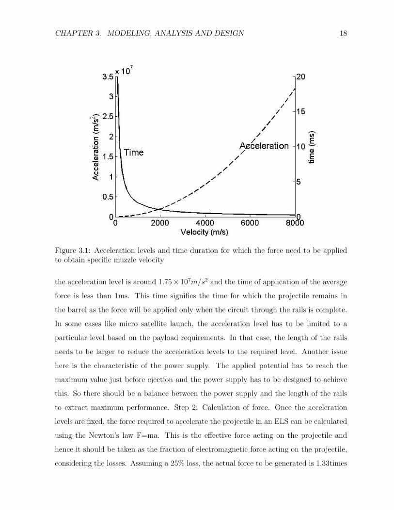
3.1 Acceleration levels and time duration for which the force need to be appliedto obtain specific muzzle velocity . . . . . . . . . . . . . . . . . . . . . . . 18
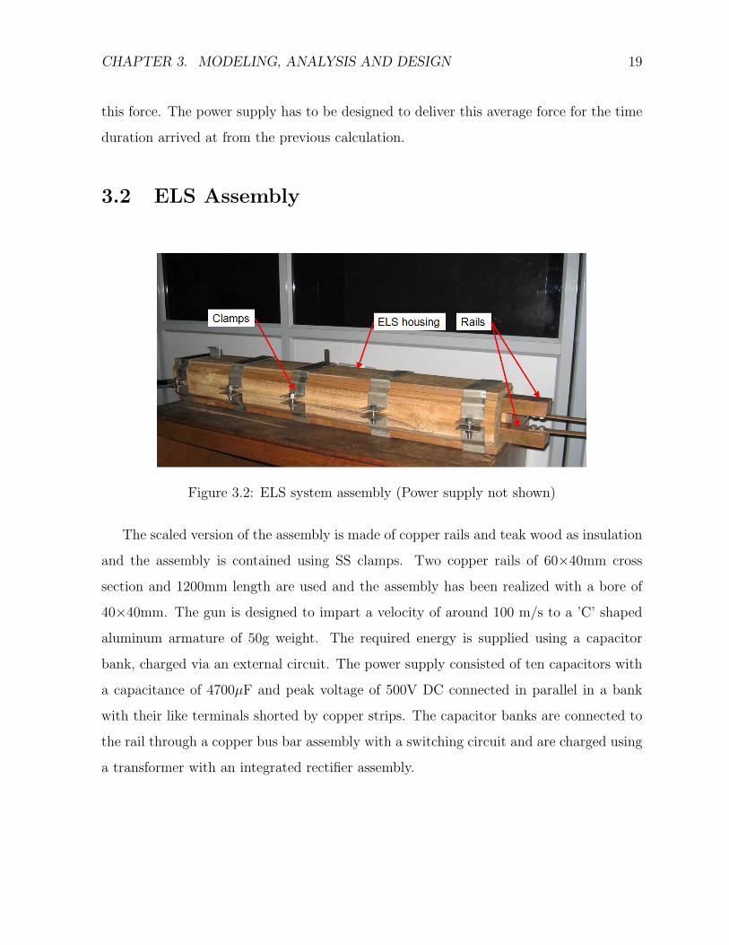
3.2 ELS system assembly (Power supply not shown) . . . . . . . . . . . . . . . 193.3 ELS 3D Model . . . . . . . . . . . . . . . . . . . . . . . . . . . . . . . . . 263.4 Reference cross section through the armature. . . . . . . . . . . . . . . . . 293.5 Reference longitudinal section through the rail. . . . . . . . . . . . . . . . 303.6 Current density through the input rail along the reference section in fig.3.5. 313.7 Current density through the output rail along the reference cross section
in fig.3.5. . . . . . . . . . . . . . . . . . . . . . . . . . . . . . . . . . . . . . 313.8 Variation of J through the armature along X direction. . . . . . . . . . . . 323.9 Surface plots of current density through the armature. (a).Section 5mm to-
wards the negative X direction from the reference cross section. (b).Section5mm towards the positive X direction from the reference cross section. . . 33
3.10 Current density through the rails and armature - Streamline plot in YZplane. . . . . . . . . . . . . . . . . . . . . . . . . . . . . . . . . . . . . . . 34
3.11 Current density through the rails and armature - Slice plot. . . . . . . . . . 343.12 Applied potential across the rails - Linearly varied input. . . . . . . . . . . 353.13 Applied potential across the rails - Exponentially varied input. . . . . . . . 363.14 Variation of Jz through the input rail along Z direction for different time
steps . . . . . . . . . . . . . . . . . . . . . . . . . . . . . . . . . . . . . . . 373.15 Variation of Jz through the output rail along Z direction for different time
steps . . . . . . . . . . . . . . . . . . . . . . . . . . . . . . . . . . . . . . . 373.16 Variation of Jx through the armature along X direction for different time
steps . . . . . . . . . . . . . . . . . . . . . . . . . . . . . . . . . . . . . . . 383.17 Force on armature for the exponentially varying potential . . . . . . . . . . 383.18 Force on rails for the exponentially varying potential . . . . . . . . . . . . 39
4.1 Simplified analytical model of ELS rail geometry . . . . . . . . . . . . . . 424.2 2D Analytical model of rail . . . . . . . . . . . . . . . . . . . . . . . . . . 434.3 Variation of wavenumber with frequency for a normal Euler Bernoulli beam 46
v
LIST OF FIGURES vi
4.4 Variation of wavenumber with frequency for an Euler Bernoulli beam onelastic foundation, neglecting rotational inertia . . . . . . . . . . . . . . . . 46
4.5 Variation of wavenumber with frequency for an Euler Bernoulli beam onelastic foundation, considering rotational inertia . . . . . . . . . . . . . . . 47
4.6 Variation of wavenumber k1 with frequency for different values of Va . . . . 484.7 Variation of wavenumber k2 with frequency for different values of Va . . . . 484.8 Variation of wavenumber k3 with frequency for different values of Va . . . . 494.9 Variation of wavenumber k4 with frequency for different values of Va . . . . 494.10 Variation of wavenumber k1 with frequency for different values of µ . . . . 504.11 Variation of wavenumber k2 with frequency for different values of µ . . . . 514.12 FE model of rail . . . . . . . . . . . . . . . . . . . . . . . . . . . . . . . . 524.13 Determinant of reduced stiffness matrix against frequency for various values
of support structure stiffness . . . . . . . . . . . . . . . . . . . . . . . . . . 554.14 Change in first mode frequency with stiffness of structural containment . . 564.15 Determinant of reduced stiffness matrix against frequency for various values
of armature velocity. . . . . . . . . . . . . . . . . . . . . . . . . . . . . . . 574.16 Variation in first mode frequency with armature velocity . . . . . . . . . . 57
5.1 Schematic of the power supply scheme for table top ELS . . . . . . . . . . 595.2 Schematic of the ELS barrel realized . . . . . . . . . . . . . . . . . . . . . 605.3 Composite housing for ELS: Assembly drawing . . . . . . . . . . . . . . . . 62
Chapter 1
Introduction
Efforts to use electromagnetism to launch objects at high velocities were started long back
in 1844. Since then many advances occurred in this field, especially with the renewed inter-
est in recent years. A railgun is the simplest device to launch projectiles of comparatively
low mass with a very high velocity, using the principle of electromagnetism. The layout of
an Electromagnetic Launch System (ELS) consists of two parallel conductive rails which
are shorted using an armature, which is free to move between the rails. When current
passes through the ELS assembly, magnetic filed will be setup and the armature and rails
experience electromagnetic force. The rails are contained using mechanical clamps and
the force on armature will eject it out of the assembly at a high velocity, depending on
the magnitude of current [1].
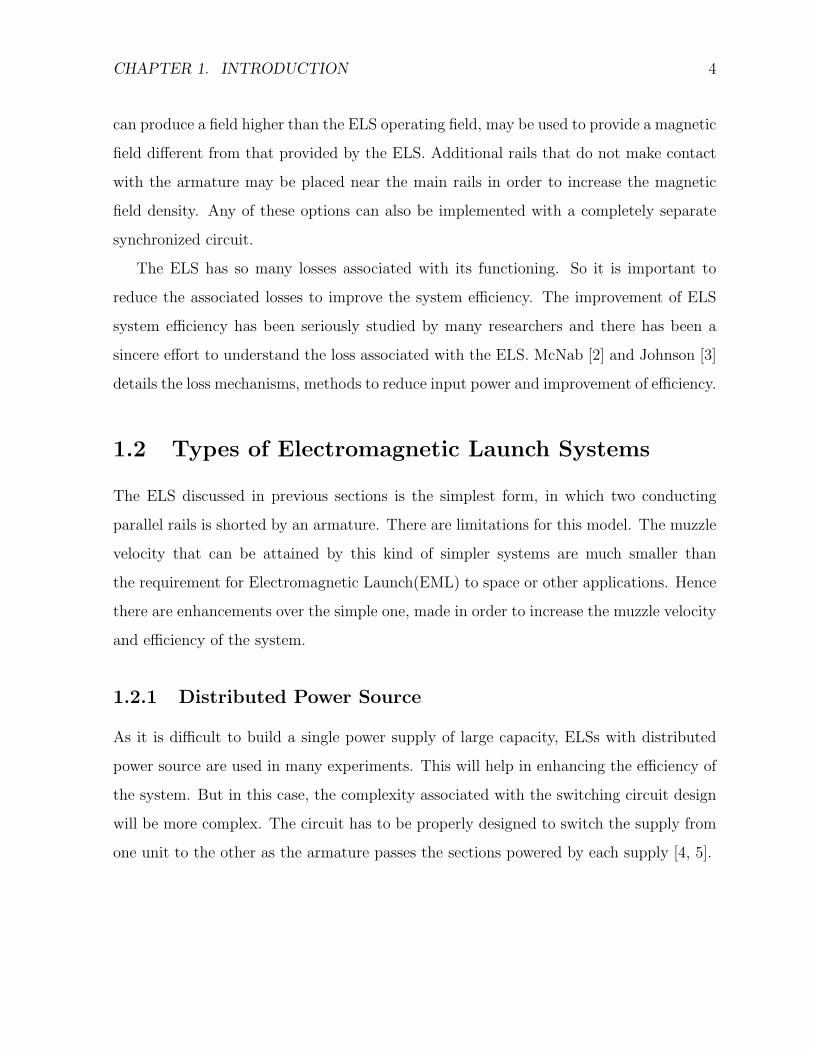
1.1 Theory of Electromagnetic Launch System(ELS)
An ELS consists of a pair of conducting rails separated by a distance and with the rails
connected to the positive and negative sides of a power source supplying a high current.
A conducting armature shorts the gap between the rails, completing the electrical circuit.
The high current through the rails sets up a magnetic filed and its interaction with the
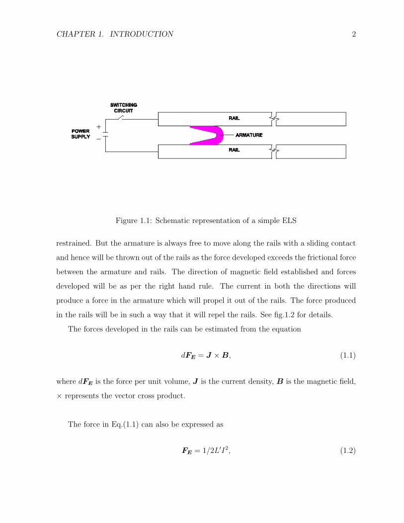
electric field produce forces on the conductors, i.e. the rails and the armature (fig.1.1).
The rails will be contained using mechanical clamps and hence movement will be
1
CHAPTER 1. INTRODUCTION 2
Figure 1.1: Schematic representation of a simple ELS
restrained. But the armature is always free to move along the rails with a sliding contact
and hence will be thrown out of the rails as the force developed exceeds the frictional force
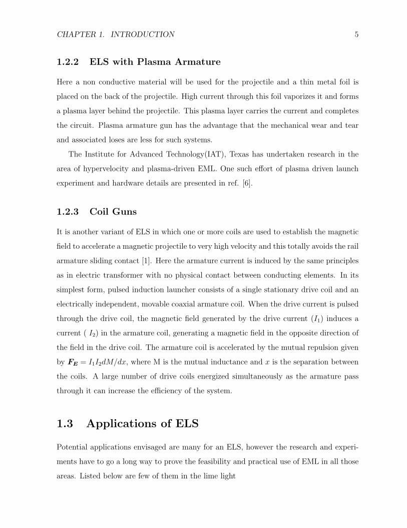
between the armature and rails. The direction of magnetic field established and forces
developed will be as per the right hand rule. The current in both the directions will
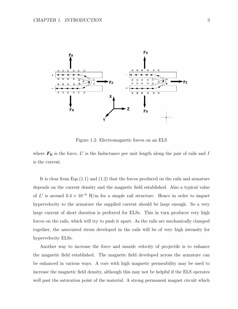
produce a force in the armature which will propel it out of the rails. The force produced
in the rails will be in such a way that it will repel the rails. See fig.1.2 for details.
The forces developed in the rails can be estimated from the equation
dFE = J ×B, (1.1)
where dFE is the force per unit volume, J is the current density, B is the magnetic field,
× represents the vector cross product.
The force in Eq.(1.1) can also be expressed as
FE = 1/2L′I2, (1.2)
CHAPTER 1. INTRODUCTION 3
Figure 1.2: Electromagnetic forces on an ELS
where FE is the force, L′ is the Inductance per unit length along the pair of rails and I
is the current.
It is clear from Eqs.(1.1) and (1.2) that the forces produced on the rails and armature
depends on the current density and the magnetic field established. Also a typical value
of L′ is around 0.4 × 10⁻⁶ H/m for a simple rail structure. Hence in order to impart
hypervelocity to the armature the supplied current should be large enough. So a very
large current of short duration is preferred for ELSs. This in turn produces very high
forces on the rails, which will try to push it apart. As the rails are mechanically clamped
together, the associated stress developed in the rails will be of very high intensity for
hypervelocity ELSs.
Another way to increase the force and muzzle velocity of projectile is to enhance
the magnetic field established. The magnetic field developed across the armature can
be enhanced in various ways. A core with high magnetic permeability may be used to
increase the magnetic field density, although this may not be helpful if the ELS operates
well past the saturation point of the material. A strong permanent magnet circuit which
CHAPTER 1. INTRODUCTION 4
can produce a field higher than the ELS operating field, may be used to provide a magnetic
field different from that provided by the ELS. Additional rails that do not make contact
with the armature may be placed near the main rails in order to increase the magnetic
field density. Any of these options can also be implemented with a completely separate
synchronized circuit.
The ELS has so many losses associated with its functioning. So it is important to
reduce the associated losses to improve the system efficiency. The improvement of ELS
system efficiency has been seriously studied by many researchers and there has been a
sincere effort to understand the loss associated with the ELS. McNab [2] and Johnson [3]
details the loss mechanisms, methods to reduce input power and improvement of efficiency.
1.2 Types of Electromagnetic Launch Systems
The ELS discussed in previous sections is the simplest form, in which two conducting
parallel rails is shorted by an armature. There are limitations for this model. The muzzle
velocity that can be attained by this kind of simpler systems are much smaller than
the requirement for Electromagnetic Launch(EML) to space or other applications. Hence
there are enhancements over the simple one, made in order to increase the muzzle velocity
and efficiency of the system.
1.2.1 Distributed Power Source
As it is difficult to build a single power supply of large capacity, ELSs with distributed
power source are used in many experiments. This will help in enhancing the efficiency of
the system. But in this case, the complexity associated with the switching circuit design
will be more complex. The circuit has to be properly designed to switch the supply from
one unit to the other as the armature passes the sections powered by each supply [4, 5].
CHAPTER 1. INTRODUCTION 5
1.2.2 ELS with Plasma Armature
Here a non conductive material will be used for the projectile and a thin metal foil is
placed on the back of the projectile. High current through this foil vaporizes it and forms
a plasma layer behind the projectile. This plasma layer carries the current and completes
the circuit. Plasma armature gun has the advantage that the mechanical wear and tear
and associated loses are less for such systems.
The Institute for Advanced Technology(IAT), Texas has undertaken research in the
area of hypervelocity and plasma-driven EML. One such effort of plasma driven launch
experiment and hardware details are presented in ref. [6].
1.2.3 Coil Guns
It is another variant of ELS in which one or more coils are used to establish the magnetic
field to accelerate a magnetic projectile to very high velocity and this totally avoids the rail
armature sliding contact [1]. Here the armature current is induced by the same principles
as in electric transformer with no physical contact between conducting elements. In its
simplest form, pulsed induction launcher consists of a single stationary drive coil and an
electrically independent, movable coaxial armature coil. When the drive current is pulsed
through the drive coil, the magnetic field generated by the drive current (I1) induces a
current ( I2) in the armature coil, generating a magnetic field in the opposite direction of
the field in the drive coil. The armature coil is accelerated by the mutual repulsion given
by FE = I1I2dM/dx, where M is the mutual inductance and x is the separation between
the coils. A large number of drive coils energized simultaneously as the armature pass
through it can increase the efficiency of the system.
1.3 Applications of ELS
Potential applications envisaged are many for an ELS, however the research and experi-
ments have to go a long way to prove the feasibility and practical use of EML in all those
areas. Listed below are few of them in the lime light
CHAPTER 1. INTRODUCTION 6
1.3.1 Military Applications
ELS is of particular interest in defense applications. These systems can replace large
artilleries and will have the advantages of being light, easy to transport and easy to handle.
Another positive factor is that because of the hypervelocity, the missiles launched using
ELS will not be that easy to intercept and the directional stability will also be better. It
is being projected as an important part of Strategic Defense Initiative (SDI) [7]. SDI is a
US government program responsible for development of a space based system to defend
attacks by ballistic missiles. ELS can be used to intercept such missiles and it can even
be used to assure protection from rogue asteroids heading towards Earth.
1.3.2 Non-military Applications
The system can be used to launch objects and micro satellites to space in a more effective
manner, once the associated technologies are fully developed. The concept of launching
material to space has been the subject of keynote presentations and several symposium
publications since the inception of the EML Symposia. The primary attraction of elec-
tromagnetic launch to space is the projected savings in the cost per kilogram of launching
material to low earth orbit. Projected savings by factors of from 300 to 1000 times ap-
pears possible, but it is clearly one of the most difficult applications of the technology.
Ian R Mcnab et. al has discussed several such issues in refs. [6], [8], [9]. The initial U.S.
interest in electromagnetic launch was stimulated by the early designs by Henry Kolm
and Gerard O’Neill of the mass driver to launch material from the surface of the moon
to a space station in earth orbit [10]. The researchers in the area sincerely believe that,
in future, low cost access and commercialization of space will be enabled by this launch
technology.
EML can also be used to initiate fusion reactions. Fusion occurs when two small
atomic nuclei combine together to form a larger nucleus, a process that releases large
amounts of energy. Atomic nuclei must be traveling at enormous velocities for this to
happen. It is proposes to use railguns to fire pellets of fusible material at each other. The
impact of the high-velocity pellets would create immense temperatures and pressures,
CHAPTER 1. INTRODUCTION 7
enabling fusion to occur. Onozuka M.et. al [11] have developed a railgun pellet injection
system for fusion experimental devices. Using a low electric energy railgun system, hy-
drogen pellet acceleration tests have been conducted to investigate the application of the
electromagnetic railgun system for high speed pellet injection into fusion plasmas.
1.4 Associated Engineering Challenges
The ELS is promising for use in different applications as discussed in previous section.
But there are many associated technologies, which need to be understood to a greater
depth. This calls for more detailed research and extensive experimental studies in this
field. Few major challenges identified are listed below.
1.4.1 Power Supply and Switching
The power supply to fire ELS must provide a very large current of short duration. It
must also operate at a high enough voltage to drive the required current and to squelch
any back emf from the armature. DC supplies such as lead-acid supplies can deliver
several thousand amperes for short duration, but are not practical for a large weapon
since a large number are needed to provide the requisite voltage and current. Capacitors
and compulsators can store very large amounts of energy and are capable of delivering
hundreds of kilo-amperes. Capacitors store energy via an electric field; compulsators
store energy mechanically in a flywheel. Compulsator stands for Compensated Pulsed
Alternator; a compulsator uses a very low inductance generator to allow for rapid current
rise and a high energy density flywheel to store energy. A compulsator can store enough
energy to fire a ELS several consecutive times where a capacitor bank usually uses all of
its energy on each shot and needs to be recharged after each shot. Compulsators generally
can store more energy per unit volume than capacitors.
The development of switching circuit for very high current with a very low switching
time of the order of micro-seconds is another problem in the ELS realization.
CHAPTER 1. INTRODUCTION 8
1.4.2 Rail Repulsion and Mechanical Wear
For any ELS the currents required will place large amounts of mechanical stress on the
current carrying parts. The current carrying bars of the rail and the connectors must be
stiff and fastened into place. If the ELS uses a plasma armature, the armature/projectile
has to be tightly fit into the barrel and the barrel will have to be sealed to keep the plasma
from escaping. For a solid armature the surface area in contact with the rails need to be
maximized and good contact should be maintained. This is necessary to reduce arcing
and spot welding and to allow for high current flow. But at the same time friction
at the rail - armature interface also causes major problems in the ELS function. The
deformation caused due to the electromagnetic forces developed can add to the problem
by increasing the friction between surfaces in contact [12]. The technology of sliding
electrical contacts for the conventional electric motors is well established. But here the
speed is limited to a maximum of 100m/sec, whereas the ELS armatures move at very
high speeds of the order of 1000 to 3000 m/sec or even more. It is difficult to design such
sliding contacts, which can maintain good electrical and mechanical contacts at these
speeds also [1]. Considerable research has gone into understanding the sliding contact
characteristics at high velocities and also there has been proposals for different designs
[13]-[15]. The armature rail interface should be designed to minimize gouging, and if any
gouging is to occur, it is more desirable to have the damage on the armature instead of
the rails, so that the rails can be reused for more launches. To achieve this, the rails
should be as hard as feasible and the armature as soft as possible. Many materials and
construction techniques have been tried to make long lasting rails. This is still an area of
significant research. When the ELS is fired the armature/projectile should be injected at
a high velocity to overcome that static friction of the barrel and to prevent spot welding.
A fast injection also will spread out the heat generated across a greater area again helping
to prolong rail life. Unless the magnetic field is supplied externally the armature should
have a sufficient length of current carrying rail behind, before it contacts the rails, in
order to allow a strong magnetic field to be created. Even then, it may be desirable to
augment the magnetic field where the armature first makes contact since the current will
CHAPTER 1. INTRODUCTION 9
not immediately begin to accelerate the armature.
Various experiments have been conducted to study the mechanical friction, the viscous
arc drag and the ablation effects. At the beginning of 1987 the French-German research
institute of Saint-Louis (ISL) started its activities on electromagnetic acceleration. ISL
has conducted research works on different kinds of fuse armatures for electromagnetic rail
launchers [16]. In articles [17, 18], the influence of an armature material on acceleration
dynamics has been investigated by means of computational methods. ELS housing also
has got considerable importance in improving the efficiency and performance. Lehmann
et. al [19] explains a comparative study on performance with different housing made of
fiber wound composites.
1.4.3 Solid Armature Transition
Even though the early ELS research started with the use of metallic armatures, this
technique was successful only for velocities up to about 1 km/s, as intermittent contact
only could be maintained at hypervelocities. This caused the interface voltage between
the armature and rails to rise from the few volts, typical of a metallic contact, to voltages
of tens to hundreds of volts as arcing contacts caused plasmas to become the path for the
current flow. This phenomenon is called transition [20]. Within the arc, temperatures up
to 30,000 K have been postulated and serious erosion of rail surfaces has been observed.
Pressures generated in the confined plasma region between the armature and the rails
has been identified as a source of observed deformation of projectile components [21].
Maintaining non arcing contact to hypervelocities with metal armatures is important
for improving efficiency, rail life and launch package integrity. Significant reduction in
armature energy loss, which is identified as a major means of energy loss in ELS, can be
achieved through the use of metal/transitioning armatures [22].
Several mechanisms that lead to armature transition have been identified and reported
in the past and a review of possible armature transition mechanisms is given by J P Barber
et. al [23]. This review indicates the complexity and multiplicity of mechanisms that can
trigger the onset of transition. For ELS, Joule heating is another major concern. Since
CHAPTER 1. INTRODUCTION 10
roughly 50% of the breech electrical energy remains in the railgun after shot exit, rail
heating is a significant concern [21].
1.5 Objectives
Though EML has so many advantages compared to conventional chemical rocket launch,
the associated complexity is also more. There are numerous theoretical as well as ex-
perimental studies being conducted at different places across the world, to increase the
launch velocity and to improve the efficiency of the system. In India, an initiative has
been taken up at IISc towards the development of electromagnetic launch technology and
a set of preliminary tests are being conducted. It is aimed to realize a table top ELS
which can accelerate a projectile of around 50 g mass to 10m/s or more. Preliminary
design has been completed and a few trials have already been carried out. This work
is aimed at developing a three dimensional model of the system to understand various
system parameters.
Lot of research work has gone into the modeling and simulation of ELS and special
finite element codes are also developed for better representation of the coupled phenomena
in ELS. The current density distribution through ELS rails and armature are extensively
studied and many literature are available [24] - [28]. Elastic waves through the rails and
change in contact pressure are studied in [29]. Experimental validation is also referred
in many literatures. EMAS, MEGA and EMAP3D are the codes widely used [30],[31]
and are copy righted codes available only to a core group. As none of these codes are
available as such for public use, one has to develop own code or use some of the available
multiphysics packages to do the modeling and simulation of ELS. More over most of the
literatures rely on 2D approximation of the problem to predict the forces on armature
and velocity induced [32]. So the present work was planned with the following objectives,
• Develop a 3D model of ELS using one of the commercially available software package
COMSOLTM.
• Study the design adequacy of the proposed ELS.
CHAPTER 1. INTRODUCTION 11
• Validation of the model using experimental results.
• Formulation of a 2D analytical model of system dynamics using Lagrangian formu-
lation, incorporating the frictional force due to the moving armature.
• To study the characteristics of axial and flexural wave propagation through the rails.
• Spectral finite element formulation and analysis of system stability at various fre-
quencies.
1.6 Overview
The report is organized as the following chapters. Chapter 2 reviews the current literature
and puts in the current status of theoretical and experimental research work being con-
ducted in this area. Modeling Analysis and design aspects are included as third chapter.
Fourth chapter explains the 2D formulation for the system and stability analysis. The
details of the experimental setup and trial runs are explained in chapter 5. A summary
of the work is added towards the end with a section on the scope for future work.
Chapter 2
Review of Literature
2.1 Electromagnetic Launch
The scientific community once believed that ELS will not be successful in achieving hy-
pervelocity. The prejudice was proved wrong by the experiments of Marshal et. al [33]
in 1970s. In their trials, around 6km/s muzzle velocity was achieved for small projectiles.
This triggered further research in the area of EML and hypervelocity and led to significant
developments in the area. Many technical challenges previously regarded as bottle necks
were solved by a series of theoretical studies, analysis, computations and experiments.
ELS basically is a dynamic electro-mechanical system whose electromagnetic, structural
and thermal properties are highly interdependent. To account for the behavior of tran-
sient electric and magnetic fields, fully time dependant three dimensional computational
simulations are required. Several such efforts have come up from different universities
and research institutes across the world, which have been successfully used for simulation
of different systems. EMAP3D is one such code for simulation of thermo-mechanically
coupled electromagnetic diffusion process.[34].
12
CHAPTER 2. REVIEW OF LITERATURE 13
2.2 Recoil Effect
There is a debate between the old Ampere-Neumann electrodynamics and the modern
relativistic electromagnetism [35]-[40] on the effect of recoil forces in ELS. As per the
modern theory, vacuum can sustain large reaction forces and recoil forces will not be
acting on the rails as such. The theory explains that the force experienced on the armature
is literally exerted by local magnetic field pressure. The electromagnetic energy travels
between the rails from the power source to the armature and the cause of the Lorentz force
on the armature is the transference of the field energy momentum to the electrons in the
metal. So the recoil force must cause a deceleration to the incoming field energy. Hence
the recoil forces will not be felt on the rails [38, 39]. On the other hand Ampere-Neumann
theory says that the recoil force will be acting in the longitudinal direction on rails and it
can cause lateral deflection and buckling. This was proved through different experiments
also. The Center for Electromagnetics Research of the North Eastern University, Boston
has conducted experiments exclusively to prove the longitudinal recoil effect [40].
2.3 Material Development
Most of the components of an electromagnetic launch system can be improved with the
use of advanced materials. A study by Urukov et. al [17] details the influence of material
properties on the armature acceleration. Prasad et. al developed improved electrical
conductors based on copper-silver alloys [41]. Because of their high strength-to-weight
ratios, composites are a critical enabling material for high-energy storage and high-power
pulsed alternators. Validation of the properties of composites is more complicated than
for conventional metals. Test methods have been identified for the composite laminate
materials, which are used in high-performance pulsed alternators [42]. Solid armatures
are typically made of copper, or more commonly, aluminum, since they must have high
electrical conductivity, be lightweight, but also be capable of high mechanical load-bearing
capacity. Zielinski has evaluated the thermo-physical properties of an aluminum alloy,
G1GAS 30, which is promising because of its increased mechanical properties [43]. A
CHAPTER 2. REVIEW OF LITERATURE 14
comparative study of railgun housings done by Lehmann et. al [19] details the advantages
of different materials for ELS housing like ceramics and composites. Katulka et. al has
done a detailed analysis on the feasibility of using high temperature materials for ELS to
improve the efficiency of the system [44]. S. Rosenwasser et. al has done commendable
work on the insulator material selection for the ELS housing, which can improve the
overall efficiency of the system [45].
2.4 Modeling and Analysis Efforts
Although substantial resources have been devoted to research in the area of ELS, prac-
tical implementation of such systems still faces some nontrivial technology challenges.
One such challenge is the modeling of ELS with extreme and complex electromechanical
environmental conditions, such as electromagnetic loading and ohmic heat source, which
are three-dimensional, transient, nonuniform, and coupled to each other. A comparison
of different formulations used for modeling ELS system is given by Rodger et. al [46].
Currently, only a limited number of computer codes are available , which are capable of
simulating the ELS environment completely. Furthermore, each nation has access to only
certain codes and each code has its own particular architecture and strengths. France and
Germany ISL uses EMAS, the United Kingdom’s DRA choose MEGA, and the United
States’ ARDEC uses EMAP3D. Recently there was an effort to coordinate the related re-
search activities with some common standards and geometries. This has probably helped
a lot towards the development and improvement of research tools for use in modeling
and analysis of ELS [30, 34]. Another concern is the huge computing power required
to solve such problems. The demand for more detailed understanding of the transient
electromechanical processes has increased the requirement for fine mesh sizes in compu-
tational codes. The number of unknowns can easily reach a million. The solution of such
problems may be beyond the capacity of even large single processor machines, requiring
the use of a parallel approach such as massive parallel processing (MPP) [20].
CHAPTER 2. REVIEW OF LITERATURE 15
2.5 Experimental Studies
Although there does not seem to be much in the way of documentation, it appears that
the first electric gun was created in 1844. Nothing more is known of the device, or even
how it worked. Clearly it did not fulfill the potential hoped for and did not replace
conventional guns.[47]. In 1944, using batteries as his power source, Joachim Hansler
created the first working railgun, which was able to propel a 10 g mass to speeds of
about 1km/s. After this there was not much development and ELS remained more of a
science fantasy than a reality until 1964 when the age of ELS truly began. That year,
MB Associates used a 28kJ capacitor to accelerate nylon cubes with a plasma arc as the
armature[48]. In this process, a fuse placed behind the projectile (nylon cube) was used to
initially complete the circuit. As the current ran through the fuse it vaporized the metal
and established the initial plasma arc. The plasma arc is moved forward by Lorentz’s
Force, and pushes the nylon cube forward along with it. Later, in 1972 researchers
at the Australian National University were able to accelerate 3 g projectiles to speed
of around 6km/s using plasma arcs and a 900kJ homopolar generator. Now developed
countries like USA, UK etc. are conducting lot of research activities in this field and
as part of it several experimental set ups are also established. Since then, there were
many efforts by individuals and organizations in developing ELS. Along with that, a
number of experiments were conducted in ELS and most of them were directed towards
understanding the complex phenomena associated with EML, like armature transition,
hypervelocity gouging, material wear, recoil effect on ELS etc.
Stefani and Parker [49] developed a hypothesis that in solid armature railguns, the
onset of gouging is determined by the hardness of the harder material and by density and
speed of sound of both the materials. Understanding of the mechanisms and control of
wear is vital for successful development of solid armatures. The team has performed a set
of experiments in which they measured the wear even at hypervelocities [50]. Addition-
ally they denitrified a set of governing parameters that affect material loss and wear from
armature. Another important phenomena studied in detail is the armature transition.
Barber et. al [14] studied different mechanisms that can trigger transition and significant
CHAPTER 2. REVIEW OF LITERATURE 16
rise in the transition onset velocity was achieved as a result of understanding the asso-
ciated mechanisms. The improved understanding in electromagnetic launch is partially
a consequence of significantly improved 3-D computational capability and partially due
to clever and careful experiments with improved diagnostics. Stefani et al. measured
melt-wave erosion on C-armatures launched in the medium caliber launcher (MCL) at
IAT and recovered the armatures after flight [51]. Using a crowbar switch at the breech
to rapidly shunt current out of the armature, they were able to interrupt the erosion and
collect the armatures for analysis. In this way, they investigated the effects of current
density and rail materials on the melt-wave erosion process. The debate on the action
of recoil forces in ELS is still alive, though the experiments conducted by the Center for
Electromagnetics Research of the North Eastern University, Boston has proved the action
of recoil forces on the longitudinal rails. [40].
Chapter 3
Modeling, Analysis and Design
A miniature ELS is being developed at Indian Institute of Science (IISc), as an initial
step towards the beginning of experimentation. The fig.3.2 below shows the photograph
of the system realized for experimentation.
3.1 ELS Design Aspects
The major design specification is the velocity of the projectile and the launch mass. The
acceleration level has to be arrived at to impart the required velocity to the projectile and
from this, the required force can be estimated. The following section explains the factors
to consider for the design and the preliminary design calculations.
Step 1: Length of rails and launch time Assuming that the projectile is initially at
rest, the acceleration that need to be imparted to it to reach the required muzzle velocity
at the time of exit from the barrel can be estimated using basic mechanics and is given by
a = V 2/2S, where V is the velocity of projectile and S is the length of the barrel. So the
limiting factors here are the length of the rail and the acceleration level. The acceleration
level depends on the time for which the force is applied to obtain the velocity; lesser the
time higher the acceleration levels.
Fig.3.1 shows the variation of acceleration levels and time of application of the force
to obtain desired muzzle velocity, using a barrel of 1m length. For 6 km/s muzzle velocity,
17
CHAPTER 3. MODELING, ANALYSIS AND DESIGN 18
Figure 3.1: Acceleration levels and time duration for which the force need to be appliedto obtain specific muzzle velocity
the acceleration level is around 1.75× 10⁷m/s2 and the time of application of the average
force is less than 1ms. This time signifies the time for which the projectile remains in
the barrel as the force will be applied only when the circuit through the rails is complete.
In some cases like micro satellite launch, the acceleration level has to be limited to a
particular level based on the payload requirements. In that case, the length of the rails
needs to be larger to reduce the acceleration levels to the required level. Another issue
here is the characteristic of the power supply. The applied potential has to reach the
maximum value just before ejection and the power supply has to be designed to achieve
this. So there should be a balance between the power supply and the length of the rails
to extract maximum performance. Step 2: Calculation of force. Once the acceleration
levels are fixed, the force required to accelerate the projectile in an ELS can be calculated
using the Newton’s law F=ma. This is the effective force acting on the projectile and
hence it should be taken as the fraction of electromagnetic force acting on the projectile,
considering the losses. Assuming a 25% loss, the actual force to be generated is 1.33times
CHAPTER 3. MODELING, ANALYSIS AND DESIGN 19
this force. The power supply has to be designed to deliver this average force for the time
duration arrived at from the previous calculation.
3.2 ELS Assembly
Figure 3.2: ELS system assembly (Power supply not shown)
The scaled version of the assembly is made of copper rails and teak wood as insulation
and the assembly is contained using SS clamps. Two copper rails of 60×40mm cross
section and 1200mm length are used and the assembly has been realized with a bore of
40×40mm. The gun is designed to impart a velocity of around 100 m/s to a ’C’ shaped
aluminum armature of 50g weight. The required energy is supplied using a capacitor
bank, charged via an external circuit. The power supply consisted of ten capacitors with
a capacitance of 4700µF and peak voltage of 500V DC connected in parallel in a bank
with their like terminals shorted by copper strips. The capacitor banks are connected to
the rail through a copper bus bar assembly with a switching circuit and are charged using
a transformer with an integrated rectifier assembly.
CHAPTER 3. MODELING, ANALYSIS AND DESIGN 20
3.3 Governing Equations
The ELS works on the interaction between electric and magnetic fields and is governed
by the two basic laws in electromagnetism, i.e the Biot- Savart’s Law and the Lorentz
Force. Biot-Savart’s law gives the magnetic field produced by flow of current through a
conductor and the equation is as follows:
dB =µ0
4π
Idl× r
r3; (3.1)
where dB is the differential contribution to the magnetic field resulting from this dif-
ferential element of wire, µ0 is the permeability of free space, I is the current, dl is a
vector, whose magnitude is the length of the differential element of the wire, and whose
direction is the direction of conventional current, r is the displacement unit vector in the
direction pointing from the wire element towards the point at which the field is being
computed, and r is the distance from the wire element to the point at which the field is
being computed.
The force on the current carrying conductor placed in a magnetic field is given by the
Lorentz force expression. Lorentz force expression is given by
FE = q(E + V ×B); (3.2)
where FE is the force, q is the charge, E is the electric field, V is the velocity of the
charged particle, B is the magnetic field and × represents vector cross product.
The ELS can be modeled as a system obeying the Maxwell’s relations,which describe
the interaction between electric and magnetic fields. The equations converted to potential
form are solved for the domain to get the scalar (φ) and vector potentials (A). Time-
dependant analysis of the system gives the values of A and φ, which can be used to
calculate the current density distribution and to predict the body forces developed. This
in turn can be used to check the muzzle velocity of the projectile. The model can be
used to study the variation in exit velocity and the system efficiency with respect to the
parameters like length of the rail, geometry of armature, rail cross section etc.
CHAPTER 3. MODELING, ANALYSIS AND DESIGN 21
Maxwell’s equations [52] are given by
∇×E = −∂B
∂t, (3.3)
∇×H = J + σE + ε∂E
∂t, (3.4)
∇.εE = ρ, (3.5)
∇.B = 0, (3.6)
where, E is the intensity of electric filed, H is the intensity of magnetic field, J is the
impressed current density, ε is the permittivity, µ is the permeability, B is the magnetic
flux density, σ is the conductivity of the medium.
The wave equations can be derived from these first order vector differential equations,
which will give the spatial and temporal dependence of fields and the wave nature of the
time varying electromagnetic fields. Substituting Eq.(3.4) to curl of Eq.(3.3) and putting
B = µH , we get
∇2E − µσ∂E
∂t− µε
∂2E
∂t2=
1
ε∇ρ + µ
∂J
∂t(3.7)
Taking curl of Eq.(3.4), we get
∇2H − µσ∂H
∂t− µε
∂2H
∂t2= −∇× J (3.8)
Eqs.(3.7) and (3.8) forms the non homogenous generalized wave equations in a simple
medium and for source free region with σ 6=0, ρ=0 and J =0, the above equation reduces
to homogenous generalized wave equations
∇2E − µσ∂E
∂t− µε
∂2E
∂t2= 0 (3.9)
CHAPTER 3. MODELING, ANALYSIS AND DESIGN 22
∇2H − µσ∂H
∂t− µε
∂2H
∂t2= 0 (3.10)
To simplify the mathematical analysis, auxiliary potential functions can be introduced.
We have ∇.B = 0. As divergent of B is zero, it can be expressed the curl of a vector
function say A. That is B = ∇ ×A, where A is called the magnetic vector potential.
Substituting to Eq.(3.3) and rearranging the terms, we get
∇× (E +∂A
∂t) = 0 (3.11)
which means that (E + ∂A/∂t) is an irrotational function, which can be expressed as the
gradient of a scalar potential. Let (E + ∂A/∂t) = −∇φ, where φ is the scalar potential
and we get the
E = −(∇φ +∂A
∂t) (3.12)
Substituting H = B/µ in Eq.(3.4), we get
∇×B = µε∂E
∂t+ µσE; (As J = 0) (3.13)
Substituting the expression for E from Eq.(3.12) and putting B = ∇×A, we get
∇2A− µε∂2A
∂t2− µσ
∂A
∂t= ∇(∇.A) + µε∇∂φ
∂t+ µσ∇φ (3.14)
Also we have ∇.E = 0 when charge density ρ =0 and we get
∇2φ +∂
∂t∇.A = 0 (3.15)
To define the vector function A we need to define the divergence also. Taking the choice
∇.A = 0, which is known as Coulomb gauge, the equation reduces to
∇2A− µε∂2A
∂t2− µσ
∂A
∂t= µε∇∂φ
∂t+ µσ∇φ (3.16)
CHAPTER 3. MODELING, ANALYSIS AND DESIGN 23
∇2φ = 0 (3.17)
Equations. (3.16) and (3.17) represents the potential form of Maxwell’s equation for
source free region with J = 0.
3.3.1 Muzzle Velocity of Projectile
The speed of a projectile is determined by several factors; the applied force, the amount of
time that force is applied, and friction. Effect of friction can only be determined through
testing. It is reasonable to assume a friction force equal to 25% of driving force. The
projectile, experiencing a net force as per Eq.(1.1), will accelerate in the direction of that
force. From Newton’s law, we have
a = FE/m; (3.18)
where a is the acceleration, FE is the force on projectile, m is the mass of projectile.
As the projectile moves, the magnetic flux through the circuit is increasing and thus
induces a back emf (electro motive force) manifested as a decrease in voltage across the
rails. The theoretical terminal velocity of the projectile is thus the point where the
induced emf has the same magnitude as the power source voltage, completely canceling
it out. Eq.(3.19) shows the equation for the magnetic flux.
φm = BA, (3.19)
where, φm is the magnetic flux, B is the magnetic flux density, A is the area.
Induced voltage V (i) is related to φm and the velocity of the projectile as per Eq.(3.20).
V (i) =dφm
dt= B
dA
dt= BW
dx
dt, (3.20)
where,V (i) is the induced voltage, dφm/dt is the time rate of change in magnetic flux,
dx/dt is the velocity of the projectile, W is the width of the rail.
CHAPTER 3. MODELING, ANALYSIS AND DESIGN 24
Since the projectile will continue to accelerate until the induced voltage is equal to
the applied, Eq.(3.21) shows the terminal velocity vmax of the projectile.
vmax = V/(BW ); (3.21)
where, vmax is the terminal velocity of projectile, V is the power source voltage.
These calculations give an idea of the theoretical maximum velocity of an ELS pro-
jectile, but the actual muzzle velocity is dictated by the length of the rails. The length of
the rails governs how long the projectile experiences the applied force and thus how long
it gets to accelerate. Assuming a constant force and thus a constant acceleration, the
time at which the projectile leaves the rails and muzzle velocity (assuming the projectile
is initially at rest) can be found using Eq.(3.22) and (3.23).
tf =√
2Sm/FE; (3.22)
vmuzzle =√
2SFE/m; (3.23)
where, vmuzzle is the muzzle velocity, S is the length of rails, FEis the force applied, m is
the mass of projectile.
These calculations ignore friction and air drag, and other associated losses due to
arcing, gouging, excessive heating and plasma formation etc. Another important factor
to be considered is the matching between rail length and the discharge characteristics of
the power supply. If the rail length is short so that the projectile leaves the rails before
the supplied energy is fully delivered, the system efficiency will be too less. On the other
hand if the rail length is too long such that the projectile remains in the barrel even after
the applied potential is dropped, there will be deceleration of the projectile.
3.4 Finite Element Simulation
None of the codes being used in countries like USA, France or Germany are available
to the public to do the simulation. It has been noted that the COMSOLTM multi
CHAPTER 3. MODELING, ANALYSIS AND DESIGN 25
physics package can be successfully used in simulating the system. The latest version of
this software has a model explaining the simulation of 3D railgun, which uses Induction
current and Multimedia DC modules together to simulate the moving field for an ELS.
The model assumes a constant potential applied across the rails and armature is modeled
as a moving conductivity path. But in actual practice the applied potential will be a time
varying one. Hence, here the PDE module of COMSOLTM is utilized in modeling the
system, which is an interactive program for solving coupled PDEs in one or more physical
domains simultaneously. In this study, the potential form of the Maxwell’s equations (Eq.
3.16 and 3.17) are solved. The armature is modeled as a static one as the primary aim is
to assess the forces developed in the armature and the mechanical stress produced as a
result of rail repulsion. The system of equations in the PDE General form of the module
are
ea∂2U
∂t2+ da
∂U
∂t+∇.Γ = F in Ω (3.24)
−n.(Γ) = G + (∂R/∂U )T µ on ∂Ω (3.25)
0 = R on ∂Ω (3.26)
where Ω is the computational domain: the union of all sub domains, ∂Ω is the domain
boundary and n is the outward unit normal vector on ∂Ω
Eq.(3.24) forms the system PDE, satisfied in domain Ω and Eqs.(3.25) and (3.26) are
the Neumann and Dirichlet boundary conditions respectively, which must be satisfied on
domain boundary ∂Ω. Γ, F , G and R are coefficients. They can be functions of the spatial
co-ordinates, the solution U or the space derivatives of U . T represents the transpose and
µ is the Lagrange multiplier. The analysis is done in static as well as time dependent mode.
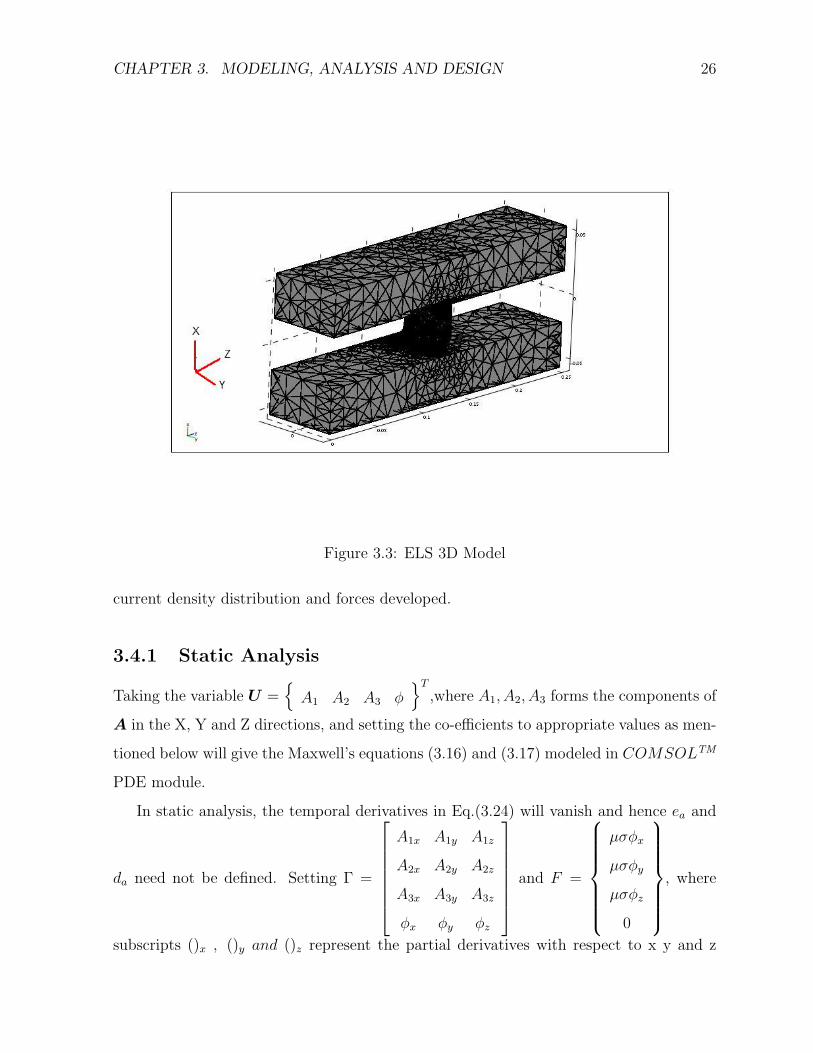
The 3D geometry is modeled in COMSOLTM with an air column around. The model
after meshing is shown in fig. 3.3. The air column around is suppressed for visualizing
the geometry in the figure.
The first attempt was to obtain the results of a static analysis in which a constant
applied potential is set between the rails and the FE solution is processed to get the
CHAPTER 3. MODELING, ANALYSIS AND DESIGN 26
Figure 3.3: ELS 3D Model
current density distribution and forces developed.
3.4.1 Static Analysis
Taking the variable U =
A1 A2 A3 φT
,where A1, A2, A3 forms the components of
A in the X, Y and Z directions, and setting the co-efficients to appropriate values as men-
tioned below will give the Maxwell’s equations (3.16) and (3.17) modeled in COMSOLTM
PDE module.
In static analysis, the temporal derivatives in Eq.(3.24) will vanish and hence ea and
da need not be defined. Setting Γ =
A1x A1y A1z
A2x A2y A2z
A3x A3y A3z
φx φy φz
and F =
µσφx
µσφy
µσφz
0
, where
subscripts ()x , ()y and ()z represent the partial derivatives with respect to x y and z
CHAPTER 3. MODELING, ANALYSIS AND DESIGN 27
respectively, will represent the set of equations 3.16 and 3.17 for the static case, in the
format of Eq.(3.24).
Boundary Conditions
Appropriate boundary conditions are; surface of air column and the rail surface which is
perpendicular to current density, is magnetic insulation. i.e. n×A = 0; and no potential
(φ = 0) condition for all the surfaces except the surface at which the potential is applied.
For that surface, φ is replaced by the constant potential to be applied.
In COMSOLTM, setting Dirichlet condition with coefficients, G =
0
4×1and
R =
A3 − A2, A1 − A3, A2 − A1, −φ + VT
, will simulate the condition. For the
input surface, V is the appropriate voltage and is zero for all other surfaces. All the
internal boundaries will have a continuity condition for the magnetic field and electric
insulation.i.e.H2−H1 = 0 and n.J = 0. In potential form this translates to n×(∇×A) =
0 and n.∇φ = 0. In the model, this can be simulated by setting Neumann boundary
condition with
G =
(−A1x − A2x − A3x), (−A1y − A2y − A3y), (−A1z − A2z − A3z), 0T
Since the length of the rail will not considerably affect the distribution of electric
and magnetic fields, a model with a length of 0.25 m for the rail is used for preliminary
studies. The position of the armature is kept at the middle of the barrel. The model
in COMSOLTM is meshed with mesh refinement for rail-armature interface. The mesh
consisted of a total of 2630 lagrange quadratic elements. The analysis is performed for a
constant voltage of 300 V applied across the rails.
3.4.2 Time-dependant Analysis
The co-efficients Γ, F , G and R cannot take time derivatives of U and hence the equations
cannot be modeled fully without going for state-space approach for variable U . To simu-
late all the boundary conditions, U is taken as
A1 A2 A3 A1dot A2dot A3dot φ φdot
T
,
where A1, A2, A3 forms the components of A in the X, Y and Z directions and A1dot A2dot A3dot
and φdot, respectively are the derivatives ofA1, A2, A3 and φ w.r.t time. By converting the
basic Maxwell’s equations to the co-efficient form, the co-efficients in Eqs.(3.24 - 3.26)
CHAPTER 3. MODELING, ANALYSIS AND DESIGN 28
takes the following form.
ea =
−µε 0 0 0 0 0 0 0
0 −µε 0 0 0 0 0 0
0 0 −µε 0 0 0 0 0
0 0 0 0 0 0 0 0
0 0 0 0 0 0 0 0
0 0 0 0 0 0 0 0
0 0 0 0 0 0 0 0
0 0 0 0 0 0 0 0
, da =
−µσ 0 0 0 0 0 0 0
0 −µσ 0 0 0 0 0 0
0 0 −µσ 0 0 0 0 0
1 0 0 0 0 0 0 0
0 1 0 0 0 0 0 0
0 0 1 0 0 0 0 0
0 0 0 0 0 0 0 0
0 0 0 0 0 0 1 0
,
Γ =
A1x A2x A3x 0 0 0 φx 0
A1y A2y A3y 0 0 0 φy 0
A1z A2z A3z 0 0 0 φz 0
T
,
F =
µεφdotx + µσφx µεφdoty + µσφy µεφdotz + µσφz A1dot A2dot A3dot 0 φdot
T
Boundary conditions
Conditions same as the static analysis case is applied here also, considering the time
derivatives in Maxwell relation. Magnetic insulation for the surface of air column and
the rail surface which is perpendicular to current density, and the zero and applied po-
tentials for the input and output surfaces transforms to the following coefficients in time
dependent PDE general form of COMSOLTM.
G =
0
8×1, R =
R1 R2 R3 R4 R5 R6 R7 R8
T
,
where R1 = A3 − A2, R2 = A1 − A3, R3 = A2 − A1, R4 = A3dot − A2dot,
R5 = A1dot − A3dot, R6 = A2dot − A1dot, R7 = −φ + V (t), R8 = −φdot + V (t),
For the far field surfaces and for the output surface, R7 and R8 are zeros. For the
input surface, V (t) is the appropriate voltage waveform and V (t) is the derivative of V (t)
w.r.t. time. Here also, all the internal boundaries will have a continuity condition for
the magnetic field and electric insulation, i.e. H2 −H1 = 0 and n.J = 0. In potential
CHAPTER 3. MODELING, ANALYSIS AND DESIGN 29
form this translates to n.(∇ ×A) = 0 and n.(∇φ + ∂A/∂t) = 0 and setting Neumann
boundary condition with
G =
G1 G2 G3 G4 G5 G6 G7 G8
T
,
where G1 = −A1x − A2x − A3x, G2 = −A1y − A2y − A3y, G3 = −A1z − A2z − A3z,
G4 = G5 = G6 = 0, G7 = A1t + A2t + A3t, G8 = 0, simulates the conditions.
3.5 Results and Discussions
3.5.1 Static Analysis
The static analysis is performed for a constant potential of 300V applied across the rails.
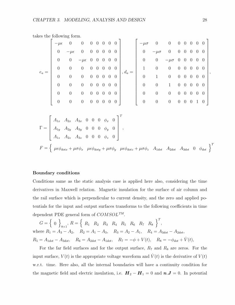
The results are discussed with reference to the fig.3.4 and 3.5. The surface marked with
1 is the surface to which positive potential is applied, which is referred as input rail and
negative potential is applied to the surface marked with 2 and is referred as output rail.
Figure 3.4: Reference cross section through the armature.
CHAPTER 3. MODELING, ANALYSIS AND DESIGN 30
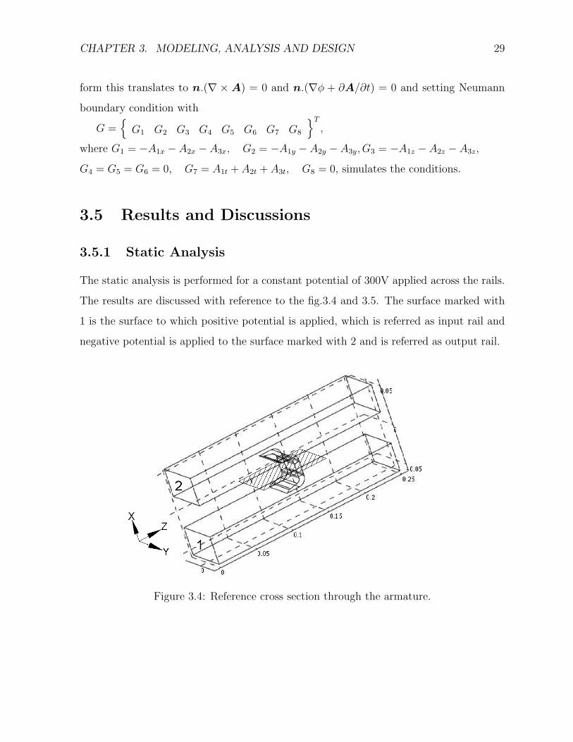
Figure 3.5: Reference longitudinal section through the rail.
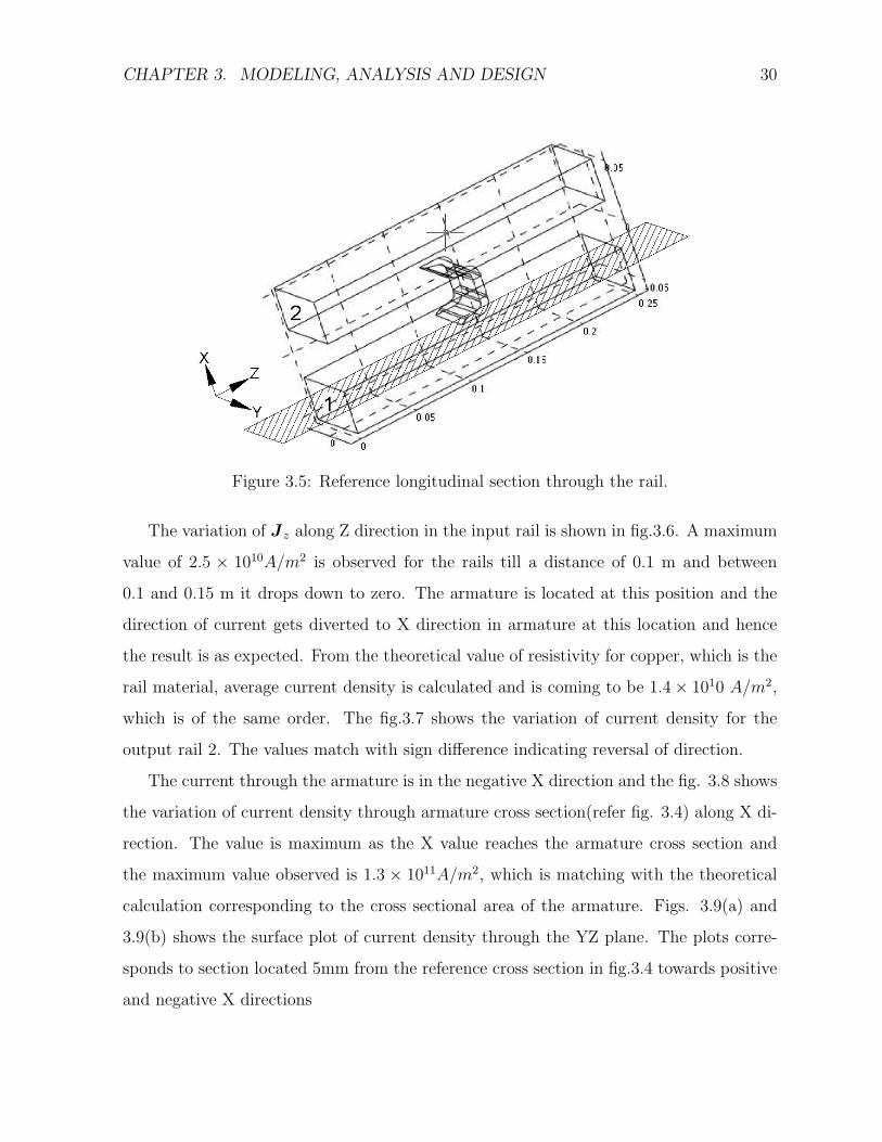
The variation of J z along Z direction in the input rail is shown in fig.3.6. A maximum
value of 2.5 × 10¹⁰A/m2 is observed for the rails till a distance of 0.1 m and between
0.1 and 0.15 m it drops down to zero. The armature is located at this position and the
direction of current gets diverted to X direction in armature at this location and hence
the result is as expected. From the theoretical value of resistivity for copper, which is the
rail material, average current density is calculated and is coming to be 1.4× 10¹⁰ A/m2,
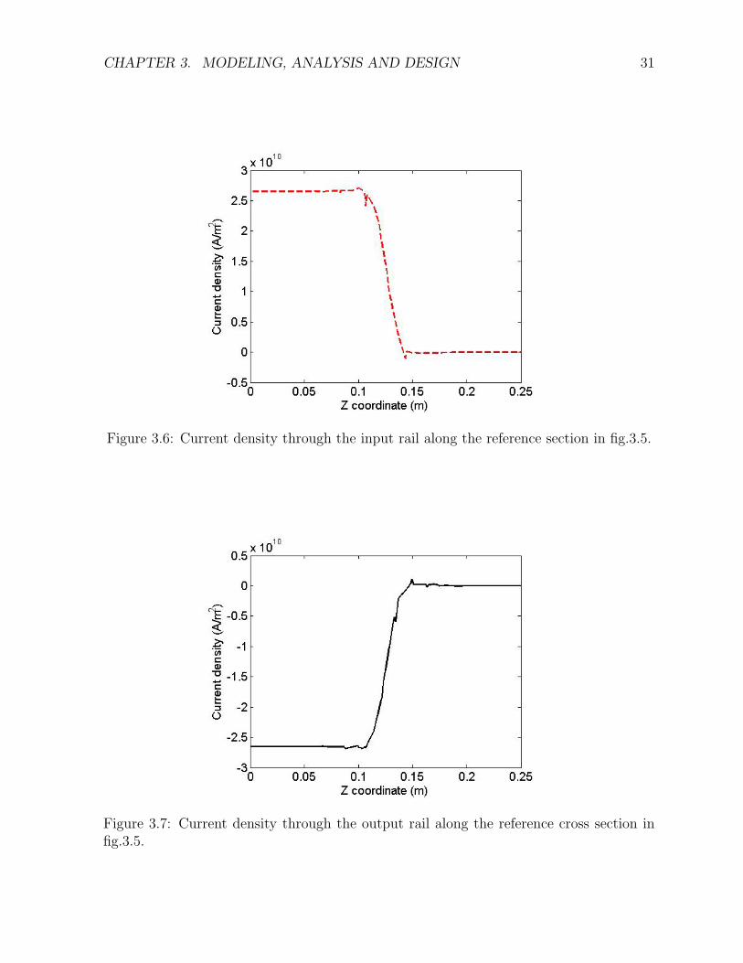
which is of the same order. The fig.3.7 shows the variation of current density for the
output rail 2. The values match with sign difference indicating reversal of direction.
The current through the armature is in the negative X direction and the fig. 3.8 shows
the variation of current density through armature cross section(refer fig. 3.4) along X di-
rection. The value is maximum as the X value reaches the armature cross section and
the maximum value observed is 1.3 × 10¹¹A/m2, which is matching with the theoretical
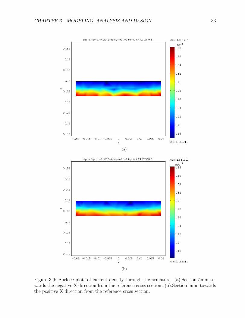
calculation corresponding to the cross sectional area of the armature. Figs. 3.9(a) and
3.9(b) shows the surface plot of current density through the YZ plane. The plots corre-
sponds to section located 5mm from the reference cross section in fig.3.4 towards positive
and negative X directions
CHAPTER 3. MODELING, ANALYSIS AND DESIGN 31
Figure 3.6: Current density through the input rail along the reference section in fig.3.5.
Figure 3.7: Current density through the output rail along the reference cross section infig.3.5.
CHAPTER 3. MODELING, ANALYSIS AND DESIGN 32
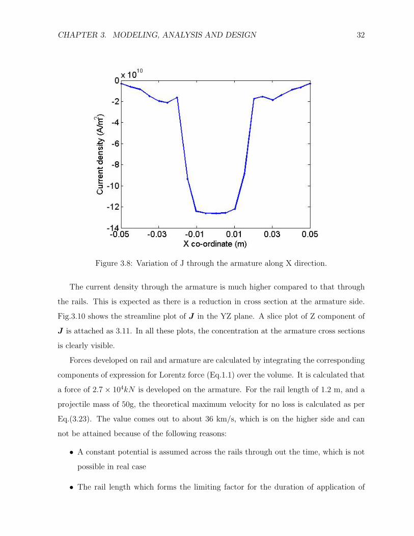
Figure 3.8: Variation of J through the armature along X direction.
The current density through the armature is much higher compared to that through
the rails. This is expected as there is a reduction in cross section at the armature side.
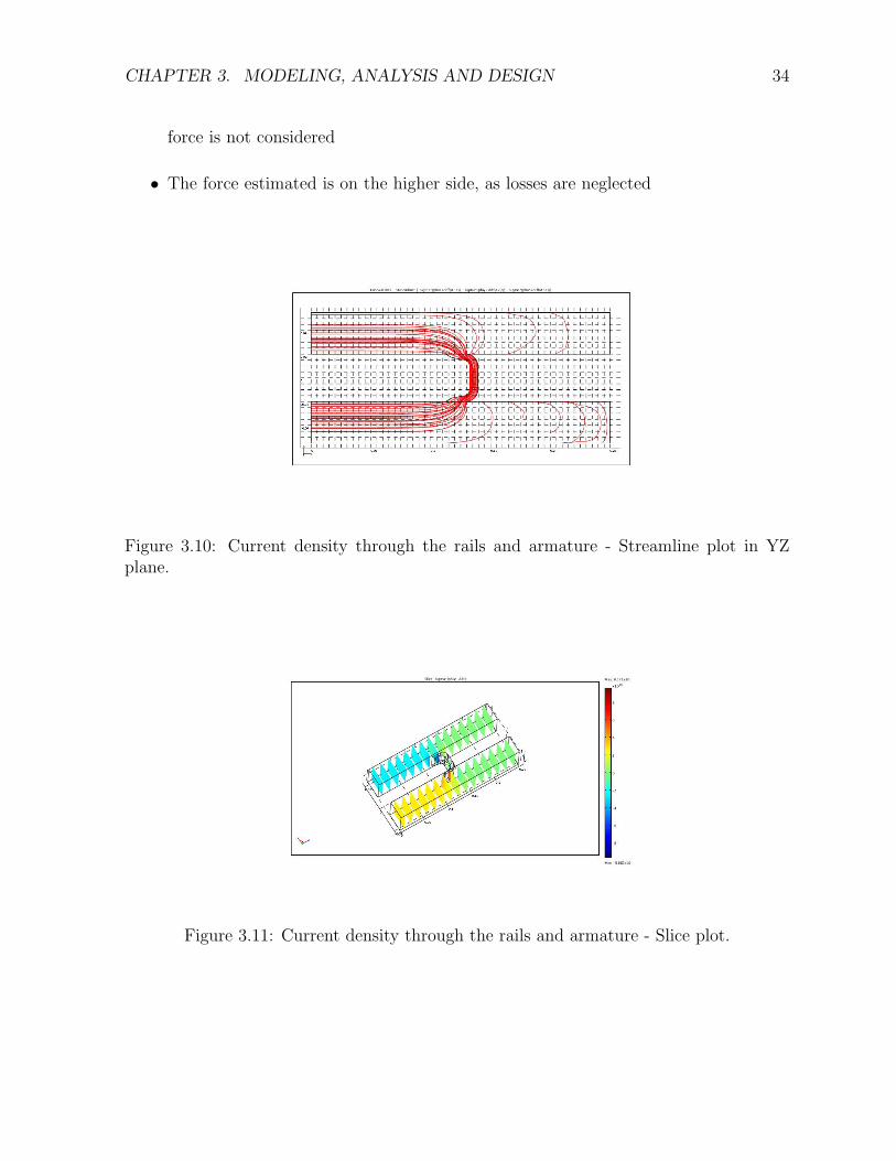
Fig.3.10 shows the streamline plot of J in the YZ plane. A slice plot of Z component of
J is attached as 3.11. In all these plots, the concentration at the armature cross sections
is clearly visible.
Forces developed on rail and armature are calculated by integrating the corresponding
components of expression for Lorentz force (Eq.1.1) over the volume. It is calculated that
a force of 2.7× 10⁴kN is developed on the armature. For the rail length of 1.2 m, and a
projectile mass of 50g, the theoretical maximum velocity for no loss is calculated as per
Eq.(3.23). The value comes out to about 36 km/s, which is on the higher side and can
not be attained because of the following reasons:
• A constant potential is assumed across the rails through out the time, which is not
possible in real case
• The rail length which forms the limiting factor for the duration of application of
CHAPTER 3. MODELING, ANALYSIS AND DESIGN 33
(a)
(b)
Figure 3.9: Surface plots of current density through the armature. (a).Section 5mm to-wards the negative X direction from the reference cross section. (b).Section 5mm towardsthe positive X direction from the reference cross section.
CHAPTER 3. MODELING, ANALYSIS AND DESIGN 34
force is not considered
• The force estimated is on the higher side, as losses are neglected
Figure 3.10: Current density through the rails and armature - Streamline plot in YZplane.
Figure 3.11: Current density through the rails and armature - Slice plot.
CHAPTER 3. MODELING, ANALYSIS AND DESIGN 35
3.5.2 Time-dependent Analysis
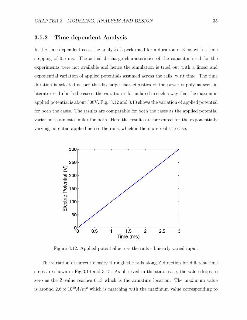
In the time dependent case, the analysis is performed for a duration of 3 ms with a time
stepping of 0.5 ms. The actual discharge characteristics of the capacitor used for the
experiments were not available and hence the simulation is tried out with a linear and
exponential variation of applied potentials assumed across the rails, w.r.t time. The time
duration is selected as per the discharge characteristics of the power supply as seen in
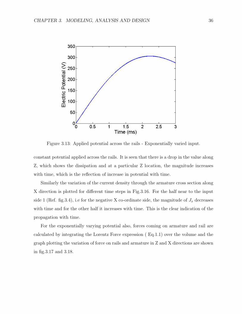
literatures. In both the cases, the variation is formulated in such a way that the maximum
applied potential is about 300V. Fig. 3.12 and 3.13 shows the variation of applied potential
for both the cases. The results are comparable for both the cases as the applied potential
variation is almost similar for both. Here the results are presented for the exponentially
varying potential applied across the rails, which is the more realistic case.
Figure 3.12: Applied potential across the rails - Linearly varied input.
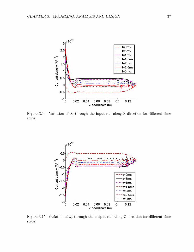
The variation of current density through the rails along Z direction for different time
steps are shown in Fig.3.14 and 3.15. As observed in the static case, the value drops to
zero as the Z value reaches 0.13 which is the armature location. The maximum value
is around 2.6 × 10¹⁰A/m2 which is matching with the maximum value corresponding to
CHAPTER 3. MODELING, ANALYSIS AND DESIGN 36
Figure 3.13: Applied potential across the rails - Exponentially varied input.
constant potential applied across the rails. It is seen that there is a drop in the value along
Z, which shows the dissipation and at a particular Z location, the magnitude increases
with time, which is the reflection of increase in potential with time.
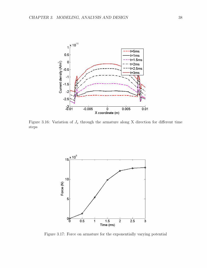
Similarly the variation of the current density through the armature cross section along
X direction is plotted for different time steps in Fig.3.16. For the half near to the input
side 1 (Ref. fig.3.4), i.e for the negative X co-ordinate side, the magnitude of Jx decreases
with time and for the other half it increases with time. This is the clear indication of the
propagation with time.
For the exponentially varying potential also, forces coming on armature and rail are
calculated by integrating the Lorentz Force expression ( Eq.1.1) over the volume and the
graph plotting the variation of force on rails and armature in Z and X directions are shown
in fig.3.17 and 3.18.
CHAPTER 3. MODELING, ANALYSIS AND DESIGN 37
Figure 3.14: Variation of Jz through the input rail along Z direction for different timesteps
Figure 3.15: Variation of Jz through the output rail along Z direction for different timesteps
CHAPTER 3. MODELING, ANALYSIS AND DESIGN 38
Figure 3.16: Variation of Jx through the armature along X direction for different timesteps
Figure 3.17: Force on armature for the exponentially varying potential
CHAPTER 3. MODELING, ANALYSIS AND DESIGN 39
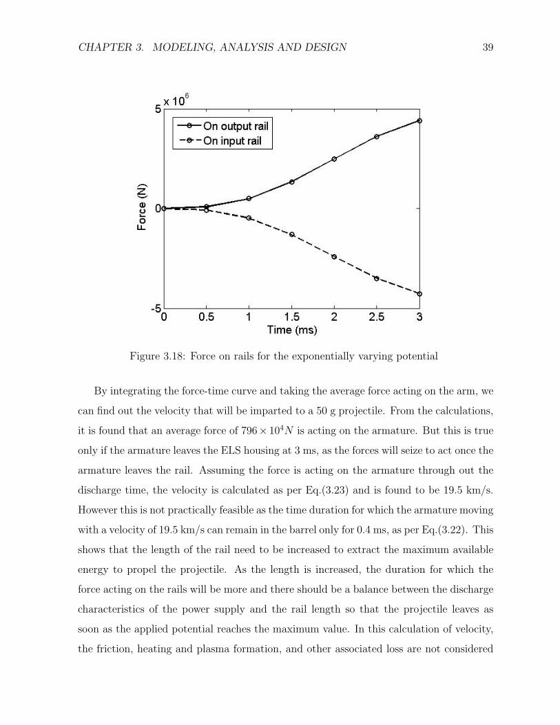
Figure 3.18: Force on rails for the exponentially varying potential
By integrating the force-time curve and taking the average force acting on the arm, we
can find out the velocity that will be imparted to a 50 g projectile. From the calculations,
it is found that an average force of 796× 104N is acting on the armature. But this is true
only if the armature leaves the ELS housing at 3 ms, as the forces will seize to act once the
armature leaves the rail. Assuming the force is acting on the armature through out the
discharge time, the velocity is calculated as per Eq.(3.23) and is found to be 19.5 km/s.
However this is not practically feasible as the time duration for which the armature moving
with a velocity of 19.5 km/s can remain in the barrel only for 0.4 ms, as per Eq.(3.22). This
shows that the length of the rail need to be increased to extract the maximum available
energy to propel the projectile. As the length is increased, the duration for which the
force acting on the rails will be more and there should be a balance between the discharge
characteristics of the power supply and the rail length so that the projectile leaves as
soon as the applied potential reaches the maximum value. In this calculation of velocity,
the friction, heating and plasma formation, and other associated loss are not considered

CHAPTER 3. MODELING, ANALYSIS AND DESIGN 40
and it is assumed that the entire force will be available to accelerate the projectile. The
quantification of associated losses can be assessed only through experiments and with that
data and the simulation results, a better approximation of the velocity can be arrived at.
Chapter 4
Analysis of System Stability
There are several problems associated with the dynamic instability of rails, coupled with
the plasma formation due to friction and arcing. As discussed in sec.1.4.3, armature
transition is one of the major problems observed in electromagnetic launchers, which can
cause severe damage to the armature and the rails of the launcher. Several studies has
been conducted on the possible explanations and studies by Johnson A J and Moon F C
[29, 54], which explains the contribution of elastic waves through the guide rail in armature
transition. Hence a similar study is envisaged here to explore the effect of frictional force
between the armature and rails in the elastic wave propagation and its effect on system
stability. The 2D analytical model is formulated by assuming the rails as a beam on
elastic foundation, and a lagrangian approach is used for incorporating the friction due
to relative movement of armature and rails.
4.1 Formulation
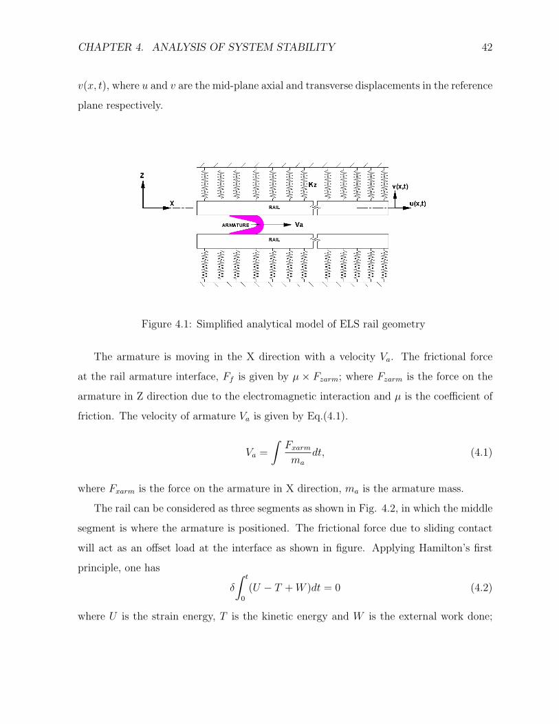
Here the conducting guide rails are modeled as an Euler Bernoulli beam and the rest of
the support structure and mechanical clamps as a classic elastic foundation as shown in
Fig. 4.1. Kz represents the stiffness per unit length of the elastic foundation, and the
assumed kinematics is that of Euler Bernoulli beam theory in which axial and transverse
displacement fields are assumed as u(x, y, z, t) = u0(x, t)− z∂v(x, t)/∂x and v(x, y, z, t) =
41
CHAPTER 4. ANALYSIS OF SYSTEM STABILITY 42
v(x, t), where u and v are the mid-plane axial and transverse displacements in the reference
plane respectively.
Figure 4.1: Simplified analytical model of ELS rail geometry
The armature is moving in the X direction with a velocity Va. The frictional force
at the rail armature interface, Ff is given by µ × Fzarm; where Fzarm is the force on the
armature in Z direction due to the electromagnetic interaction and µ is the coefficient of
friction. The velocity of armature Va is given by Eq.(4.1).
Va =
∫Fxarm
ma
dt, (4.1)
where Fxarm is the force on the armature in X direction, ma is the armature mass.
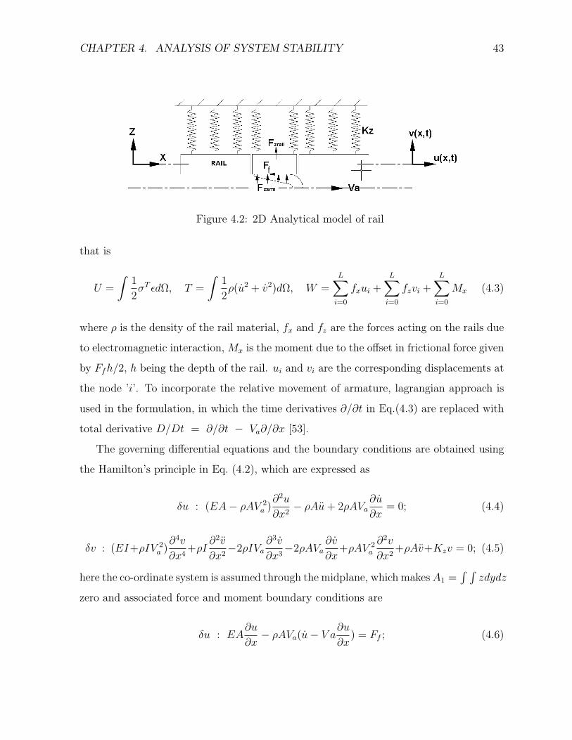
The rail can be considered as three segments as shown in Fig. 4.2, in which the middle
segment is where the armature is positioned. The frictional force due to sliding contact
will act as an offset load at the interface as shown in figure. Applying Hamilton’s first
principle, one has
δ
∫0
t
(U − T + W )dt = 0 (4.2)
where U is the strain energy, T is the kinetic energy and W is the external work done;
CHAPTER 4. ANALYSIS OF SYSTEM STABILITY 43
Figure 4.2: 2D Analytical model of rail
that is
U =
∫1
2σT εdΩ, T =
∫1
2ρ(u2 + v2)dΩ, W =
L∑i=0
fxui +L∑
i=0
fzvi +L∑
i=0
Mx (4.3)
where ρ is the density of the rail material, fx and fz are the forces acting on the rails due
to electromagnetic interaction, Mx is the moment due to the offset in frictional force given
by Ffh/2, h being the depth of the rail. ui and vi are the corresponding displacements at
the node ’i’. To incorporate the relative movement of armature, lagrangian approach is
used in the formulation, in which the time derivatives ∂/∂t in Eq.(4.3) are replaced with
total derivative D/Dt = ∂/∂t − Va∂/∂x [53].
The governing differential equations and the boundary conditions are obtained using
the Hamilton’s principle in Eq. (4.2), which are expressed as
δu : (EA− ρAV 2a )
∂2u
∂x2− ρAu + 2ρAVa
∂u
∂x= 0; (4.4)
δv : (EI+ρIV 2a )
∂4v
∂x4+ρI
∂2v
∂x2−2ρIVa
∂3v
∂x3−2ρAVa
∂v
∂x+ρAV 2
a
∂2v
∂x2+ρAv+Kzv = 0; (4.5)
here the co-ordinate system is assumed through the midplane, which makes A1 =∫ ∫
zdydz
zero and associated force and moment boundary conditions are
δu : EA∂u
∂x− ρAVa(u− V a
∂u
∂x) = Ff ; (4.6)
CHAPTER 4. ANALYSIS OF SYSTEM STABILITY 44
δv : (EI + ρIV 2a )
∂3v
∂x3− 2ρIVa
∂2v
∂x2+ ρAV 2
a
∂v
∂x− ρAVav + ρI
∂v
∂x= Fz; (4.7)
δ(∂v/∂x) : (EI − ρIV 2a )
∂2v
∂x2+ ρIVa
∂v
∂x= Ffh/2; (4.8)
where, [A I] =∫ ∫
[1 z2]dy dz, E is the modulus of elasticity, ρ is the mass density of the
rail material, Kz is the stiffness/unit length of the structural containment of rails, Fz is
the Lorenz Force on rail in Z direction and Ff is the frictional force at the rail-armature
interface.
Now that the governing equations for the assumed model are available, one can study
the characteristics of the elastic wave propagation through the structure. This will help
in identifying the effect of frictional force on wave propagation through the rails and also
the possible instabilities that can be caused due to the friction. The Eqs.(4.4) and (4.5)
are totally decoupled and hence are considered separately to study the behavior of axial
and flexural wave propagation through the rails.
4.1.1 Flexural Wave Characteristics
Spectral formulation for the system can be arrived at by assuming a solution of the form
v(x, t) =∑
vn(x, ω)eiωnt and taking vn = Bne−iknx for Eq.(4.5), where kn represents the
wavenumber corresponding to nth mode. Thus we get the characteristic equation for the
flexural wave as a 4th order polynomial in kn given by Eq.(4.9).
a1k4n + a2k
3n + a3k
2n + a4kn + a5 = 0; (4.9)
where,
a1 = EI+ρIV 2a , a2 = 2ρIVaωn, a3 = ρIω2
n−ρAV 2a , a4 = −2ρAVaωn, a5 = Kz−ρAω2
n
From Eq.(4.9), it is clear that there will be four distinct modes of waves for all non zero
values of ωn. As ωn → 0, the Eq.(4.9) will become a quadratic in k2n, which will give two
CHAPTER 4. ANALYSIS OF SYSTEM STABILITY 45
conjugate pair of roots given by Eq.(4.10).
k2n =
ρAV 2a
2(EI + ρIV 2a )±
√ρ2A2V 4
a − 4Kz(EI + ρIV 2a )
2(EI + ρIV 2a )
(4.10)
From Eq.(4.10), it is clear that for Va = 0, the roots are purely imaginary and there is no
wave propagation. For non-zero Va the roots are complex and it shows the presence of all
the four modes. As ωn → ∞, kn is given by Eq.(4.11), which is the typical behavior of
flexural waves in beams.
kn = ±
√ρA
ρI(4.11)
The frequency at which there is no wave propagation is estimated by substituting kn = 0
in Eq.(4.9)and is given by
ωcut−off =
√Kz
ρA(4.12)
The Eq.(4.9) can be solved for wavenumber kn for a given material and geometry of the
rails, over a range of frequency. The cut-off frequency for the given geometry is 10.07kHz.
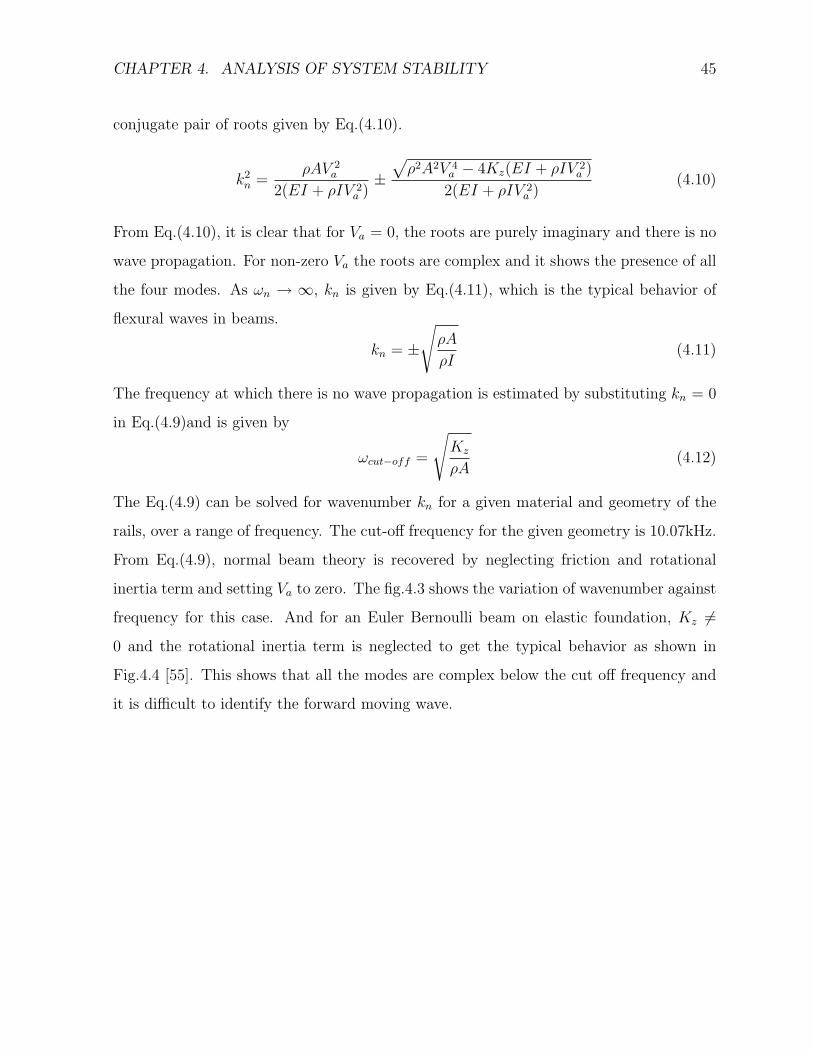
From Eq.(4.9), normal beam theory is recovered by neglecting friction and rotational
inertia term and setting Va to zero. The fig.4.3 shows the variation of wavenumber against
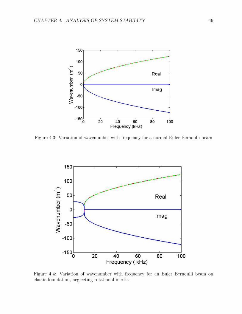
frequency for this case. And for an Euler Bernoulli beam on elastic foundation, Kz 6=
0 and the rotational inertia term is neglected to get the typical behavior as shown in
Fig.4.4 [55]. This shows that all the modes are complex below the cut off frequency and
it is difficult to identify the forward moving wave.
CHAPTER 4. ANALYSIS OF SYSTEM STABILITY 46
Figure 4.3: Variation of wavenumber with frequency for a normal Euler Bernoulli beam
Figure 4.4: Variation of wavenumber with frequency for an Euler Bernoulli beam onelastic foundation, neglecting rotational inertia
CHAPTER 4. ANALYSIS OF SYSTEM STABILITY 47
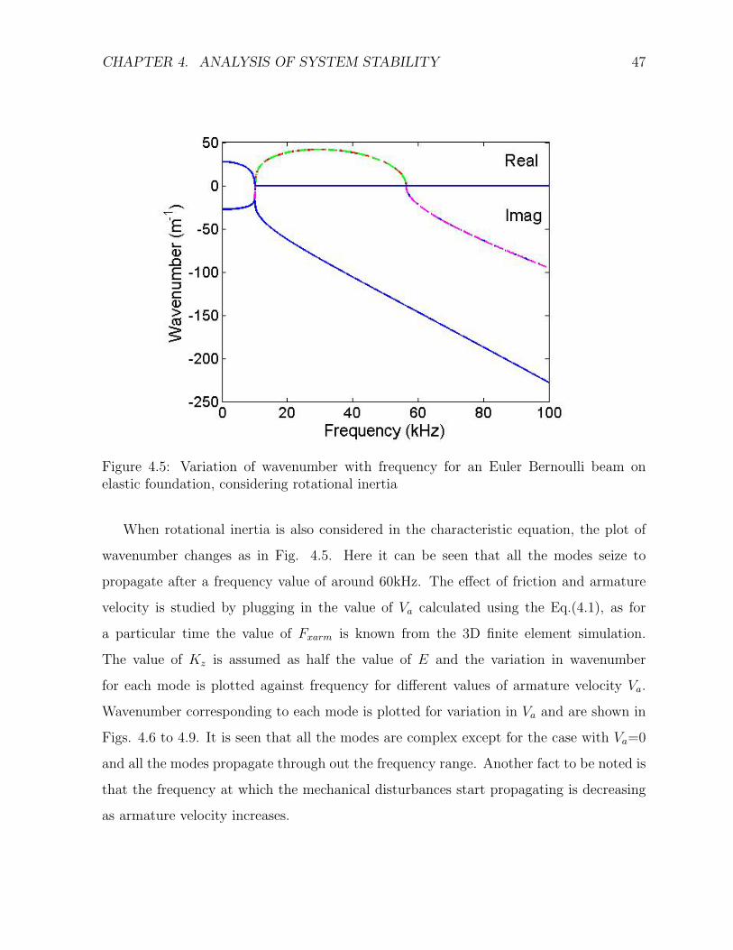
Figure 4.5: Variation of wavenumber with frequency for an Euler Bernoulli beam onelastic foundation, considering rotational inertia
When rotational inertia is also considered in the characteristic equation, the plot of
wavenumber changes as in Fig. 4.5. Here it can be seen that all the modes seize to
propagate after a frequency value of around 60kHz. The effect of friction and armature
velocity is studied by plugging in the value of Va calculated using the Eq.(4.1), as for
a particular time the value of Fxarm is known from the 3D finite element simulation.
The value of Kz is assumed as half the value of E and the variation in wavenumber
for each mode is plotted against frequency for different values of armature velocity Va.
Wavenumber corresponding to each mode is plotted for variation in Va and are shown in
Figs. 4.6 to 4.9. It is seen that all the modes are complex except for the case with Va=0
and all the modes propagate through out the frequency range. Another fact to be noted is
that the frequency at which the mechanical disturbances start propagating is decreasing
as armature velocity increases.
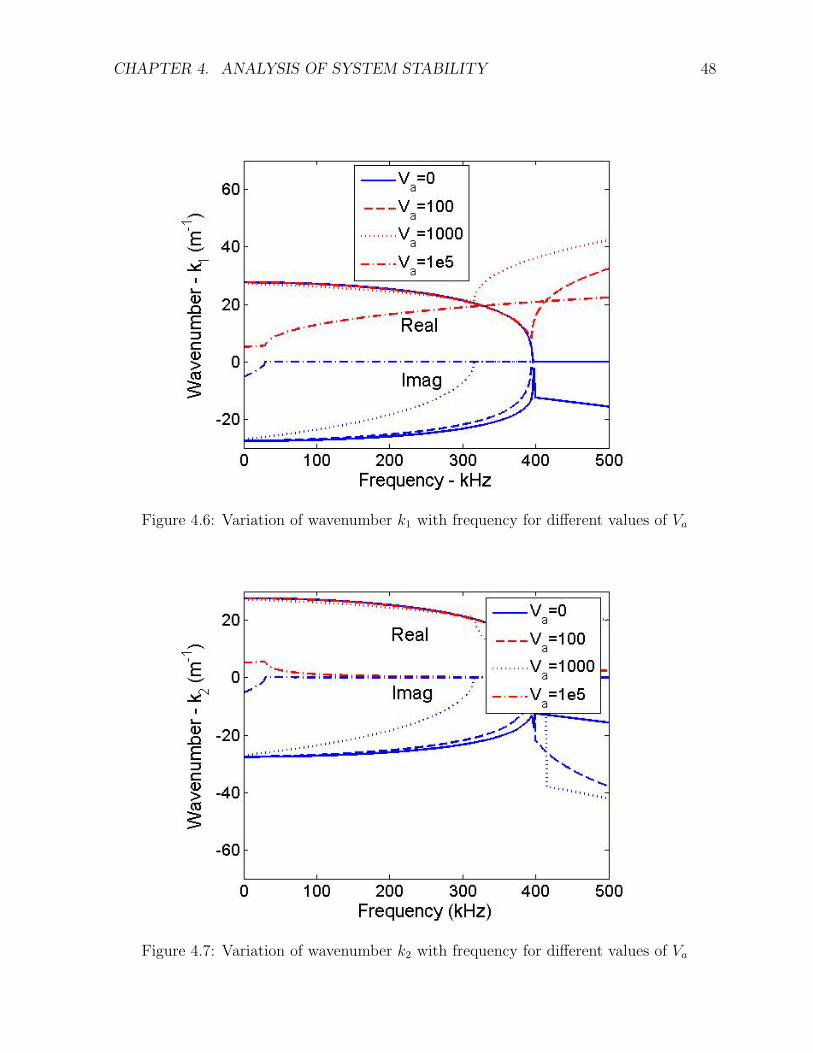
CHAPTER 4. ANALYSIS OF SYSTEM STABILITY 48
Figure 4.6: Variation of wavenumber k1 with frequency for different values of Va
Figure 4.7: Variation of wavenumber k2 with frequency for different values of Va
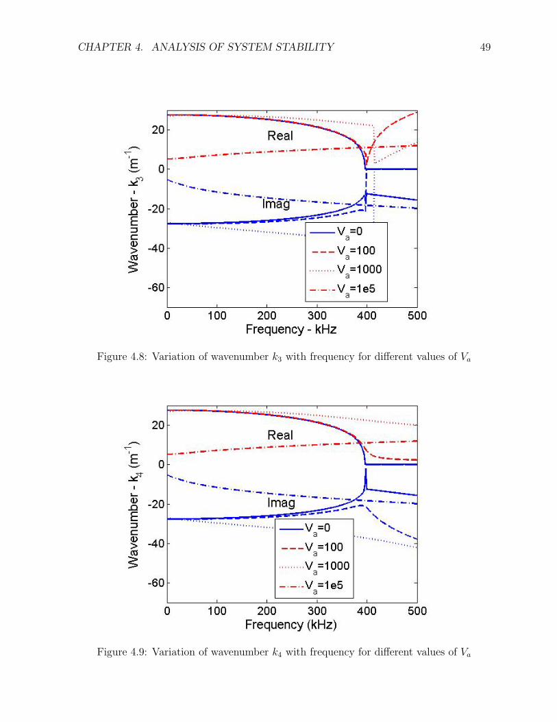
CHAPTER 4. ANALYSIS OF SYSTEM STABILITY 49
Figure 4.8: Variation of wavenumber k3 with frequency for different values of Va
Figure 4.9: Variation of wavenumber k4 with frequency for different values of Va
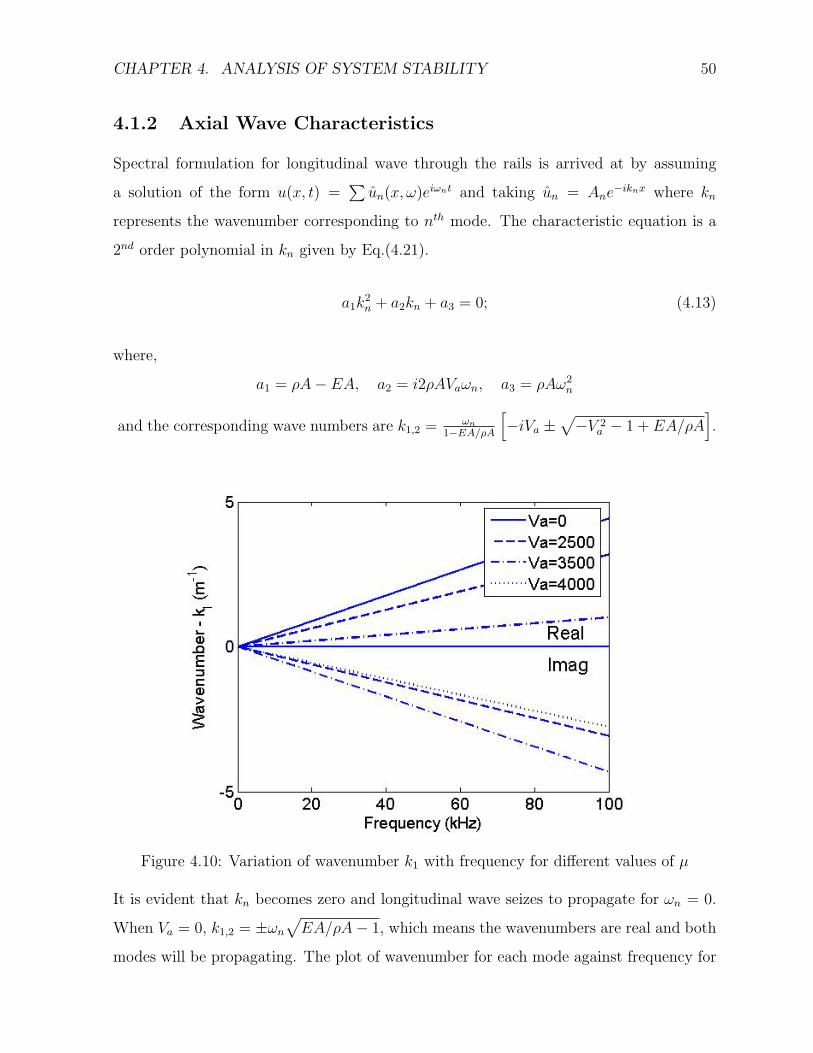
CHAPTER 4. ANALYSIS OF SYSTEM STABILITY 50
4.1.2 Axial Wave Characteristics
Spectral formulation for longitudinal wave through the rails is arrived at by assuming
a solution of the form u(x, t) =∑
un(x, ω)eiωnt and taking un = Ane−iknx where kn
represents the wavenumber corresponding to nth mode. The characteristic equation is a
2nd order polynomial in kn given by Eq.(4.21).
a1k2n + a2kn + a3 = 0; (4.13)
where,
a1 = ρA− EA, a2 = i2ρAVaωn, a3 = ρAω2n
and the corresponding wave numbers are k1,2 = ωn
1−EA/ρA
[−iVa ±
√−V 2
a − 1 + EA/ρA].
Figure 4.10: Variation of wavenumber k1 with frequency for different values of µ
It is evident that kn becomes zero and longitudinal wave seizes to propagate for ωn = 0.
When Va = 0, k1,2 = ±ωn
√EA/ρA− 1, which means the wavenumbers are real and both
modes will be propagating. The plot of wavenumber for each mode against frequency for
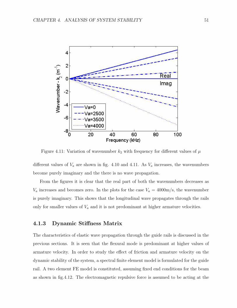
CHAPTER 4. ANALYSIS OF SYSTEM STABILITY 51
Figure 4.11: Variation of wavenumber k2 with frequency for different values of µ
different values of Va are shown in fig. 4.10 and 4.11. As Va increases, the wavenumbers
become purely imaginary and the there is no wave propagation.
From the figures it is clear that the real part of both the wavenumbers decreases as
Va increases and becomes zero. In the plots for the case Va = 4000m/s, the wavenumber
is purely imaginary. This shows that the longitudinal wave propagates through the rails
only for smaller values of Va and it is not predominant at higher armature velocities.
4.1.3 Dynamic Stiffness Matrix
The characteristics of elastic wave propagation through the guide rails is discussed in the
previous sections. It is seen that the flexural mode is predominant at higher values of
armature velocity. In order to study the effect of friction and armature velocity on the
dynamic stability of the system, a spectral finite element model is formulated for the guide
rail. A two element FE model is constituted, assuming fixed end conditions for the beam
as shown in fig.4.12. The electromagnetic repulsive force is assumed to be acting at the
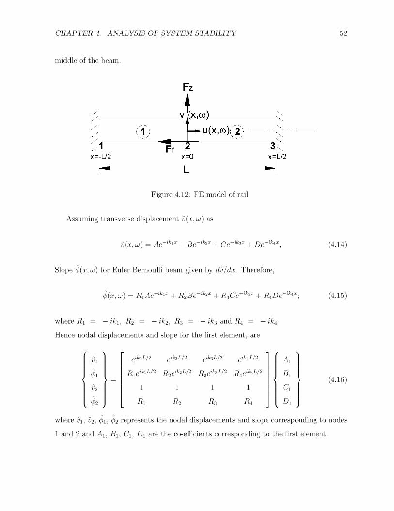
CHAPTER 4. ANALYSIS OF SYSTEM STABILITY 52
middle of the beam.
Figure 4.12: FE model of rail
Assuming transverse displacement v(x, ω) as
v(x, ω) = Ae−ik1x + Be−ik2x + Ce−ik3x + De−ik4x, (4.14)
Slope φ(x, ω) for Euler Bernoulli beam given by dv/dx. Therefore,
φ(x, ω) = R1Ae−ik1x + R2Be−ik2x + R3Ce−ik3x + R4De−ik4x; (4.15)
where R1 = − ik1, R2 = − ik2, R3 = − ik3 and R4 = − ik4
Hence nodal displacements and slope for the first element, are
v1
φ1
v2
φ2
=
eik1L/2 eik2L/2 eik3L/2 eik4L/2
R1eik1L/2 R2e
ik2L/2 R3eik3L/2 R4e
ik4L/2
1 1 1 1
R1 R2 R3 R4
A1
B1
C1
D1
(4.16)
where v1, v2, φ1, φ2 represents the nodal displacements and slope corresponding to nodes
1 and 2 and A1, B1, C1, D1 are the co-efficients corresponding to the first element.
CHAPTER 4. ANALYSIS OF SYSTEM STABILITY 53
This can be re arranged as
A1
B1
C1
D1
=
eik1L/2 eik2L/2 eik3L/2 eik4L/2
R1eik1L/2 R2e
ik2L/2 R3eik3L/2 R4e
ik4L/2
1 1 1 1
R1 R2 R3 R4
−1
v1
φ1
v2
φ2
(4.17)
Similarly for the second element
v2
φ2
v3
φ3
=
1 1 1 1
R1 R2 R3 R4
e−ik1L/2 e−ik2L/2 e−ik3L/2 e−ik4L/2
R1e−ik1L/2 R2e
−ik2L/2 R3e−ik3L/2 R4e
−ik4L/2
A2
B2
C2
D2
, (4.18)
where v2, v3, φ2, φ3 represents the nodal displacements and slope corresponding to node
2 and 3 and A2, B2, C2, D2 are the co-efficients corresponding to the second element.
Eq.(4.18) on rearranging gives
A2
B2
C2
D2
=
1 1 1 1
R1 R2 R3 R4
e−ik1L/2 e−ik2L/2 e−ik3L/2 e−ik4L/2
R1e−ik1L/2 R2e
−ik2L/2 R3e−ik3L/2 R4e
−ik4L/2
−1
v2
φ2
v3
φ3
, (4.19)
Substituting v(x, t) =∑
vn(x, ω)eiωnt in Eqs.(4.7) and (4.8) gives the expression for
shear force V (x, ω) and bending moment M(x, ω) as follows
V (x, ωn) = (EI + ρIV 2a )
d3v
dx3− i2ρIVaωn
d2v
dx2+ (ρAV 2
a − ρIω2n)
dv
dx− iρAVav, (4.20)
M(x, ωn) = (EI − ρIV 2a )
d2v
dx2+ iρIVaωn
dv
dx, (4.21)
For element 1, the V , M at the node points are obtained as
CHAPTER 4. ANALYSIS OF SYSTEM STABILITY 54
V1
M1
V2
M2
=
c11e
ik1L/2 c12eik2L/2 c13e
ik3L/2 c14eik4L/2
c21eik1L/2 c22e
ik2L/2 c23eik3L/2 c24e
ik4L/2
−c11 −c12 −c13 −c14
−c21 −c22 −c23 −c24
A1
B1
C1
D1
, (4.22)
where
c11 = −i [(EI + ρIV 2a )k3
1 + 2ρIVaωnk21 − (ρAV 2
a − ρIω2n)k1 − ρAVa]
c12 = −i [(EI + ρIV 2a )k3
2 + 2ρIVaωnk22 − (ρAV 2
a − ρIω2n)k2 − ρAVa]
c13 = −i [(EI + ρIV 2a )k3
3 + 2ρIVaωnk23 − (ρAV 2
a − ρIω2n)k3 − ρAVa]
c14 = −i [(EI + ρIV 2a )k3
4 + 2ρIVaωnk24 − (ρAV 2
a − ρIω2n)k4 − ρAVa]
c21 = (EI − ρIV 2a )k2
1 − ρIVaωnk1
c22 = (EI − ρIV 2a )k2
2 − ρIVaωnk2
c23 = (EI − ρIV 2a )k2
3 − ρIVaωnk3
c24 = (EI − ρIV 2a )k2
4 − ρIVaωnk4
Similarly for second element, we can write
V2
M2
V3
M3
=
c11 c12 c13 c14
c21 c22 c23 c24
−c11e−ik1L/2 −c12e
−ik2L/2 −c13e−ik3L/2 −c14e
−ik4L/2
−c21e−ik1L/2 −c22e
−ik2L/2 −c23e−ik3L/2 −c24e
−ik4L/2
A2
B2
C2
D2
,
(4.23)
where the constants take the same value as in Eq.(4.22)
Substituting the expressions for co-efficients A1, B1, C1, D1 from Eq.(4.17) to
Eq.(4.22) and A2, B2, C2, D2 from Eq.(4.19) to Eq.(4.23), Vn and Mn can be ex-
pressed in terms of the nodal displacements and slopes, which gives the individual stiffness
matrix for the elements. And by assembling the individual stiffness matrix for each ele-
ment,we get the global stiffness matrix of the form
V1 M1 V2 M2 V3 M3
T
=[
K]
6×6
v1 φ1 v2 φ2 v3 φ3
T
(4.24)
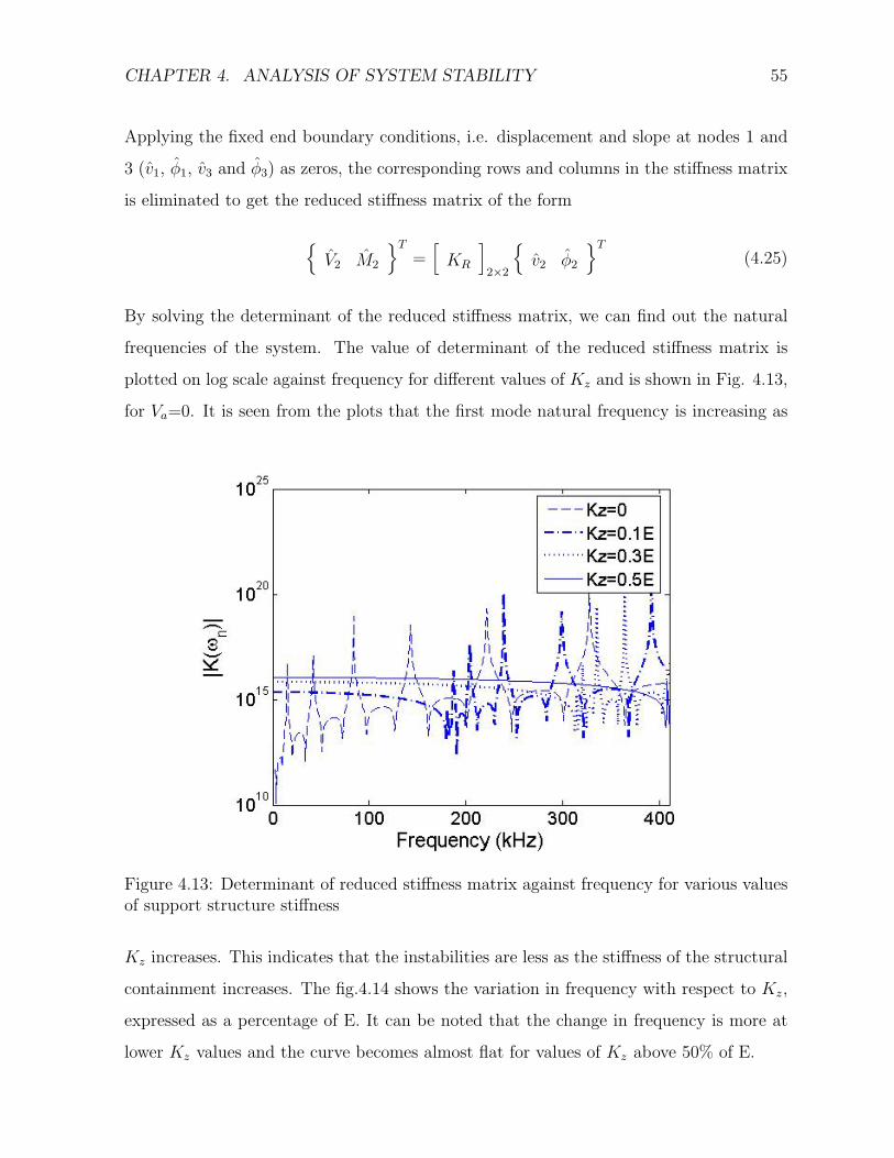
CHAPTER 4. ANALYSIS OF SYSTEM STABILITY 55
Applying the fixed end boundary conditions, i.e. displacement and slope at nodes 1 and
3 (v1, φ1, v3 and φ3) as zeros, the corresponding rows and columns in the stiffness matrix
is eliminated to get the reduced stiffness matrix of the form
V2 M2
T
=[
KR
]2×2
v2 φ2
T
(4.25)
By solving the determinant of the reduced stiffness matrix, we can find out the natural
frequencies of the system. The value of determinant of the reduced stiffness matrix is
plotted on log scale against frequency for different values of Kz and is shown in Fig. 4.13,
for Va=0. It is seen from the plots that the first mode natural frequency is increasing as
Figure 4.13: Determinant of reduced stiffness matrix against frequency for various valuesof support structure stiffness
Kz increases. This indicates that the instabilities are less as the stiffness of the structural
containment increases. The fig.4.14 shows the variation in frequency with respect to Kz,
expressed as a percentage of E. It can be noted that the change in frequency is more at
lower Kz values and the curve becomes almost flat for values of Kz above 50% of E.
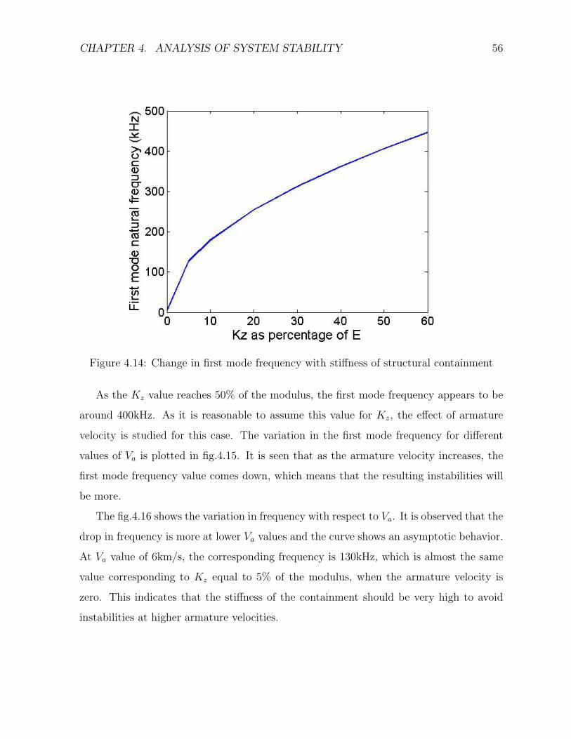
CHAPTER 4. ANALYSIS OF SYSTEM STABILITY 56
Figure 4.14: Change in first mode frequency with stiffness of structural containment
As the Kz value reaches 50% of the modulus, the first mode frequency appears to be
around 400kHz. As it is reasonable to assume this value for Kz, the effect of armature
velocity is studied for this case. The variation in the first mode frequency for different
values of Va is plotted in fig.4.15. It is seen that as the armature velocity increases, the
first mode frequency value comes down, which means that the resulting instabilities will
be more.
The fig.4.16 shows the variation in frequency with respect to Va. It is observed that the
drop in frequency is more at lower Va values and the curve shows an asymptotic behavior.
At Va value of 6km/s, the corresponding frequency is 130kHz, which is almost the same
value corresponding to Kz equal to 5% of the modulus, when the armature velocity is
zero. This indicates that the stiffness of the containment should be very high to avoid
instabilities at higher armature velocities.
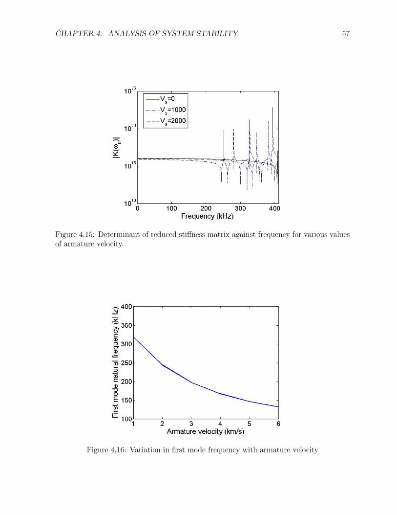
CHAPTER 4. ANALYSIS OF SYSTEM STABILITY 57
Figure 4.15: Determinant of reduced stiffness matrix against frequency for various valuesof armature velocity.
Figure 4.16: Variation in first mode frequency with armature velocity
Chapter 5
Experimental Setup
The development activities for a table top ELS for launching small projectiles of 50g size
is in progress at the high enthalpy laboratory of Department of Aerospace Engineering
at IISc. The basic idea is to study various issues associated with the launch and to
understand the complex physical phenomena associated with EML, like recoil, armature
transition, effect of various system parameters on the performance and efficiency of the
system etc. The following are the preliminary design specifications for the system under
development.
• Length of rails < 2 m
• Projectile mass ' 50 g
• Muzzle Velocity > 10 m/s
• Muzzle Energy > 2.5 J
• Average Acceleration > 25 m/s2
• Launch Time < 0.4 ms
5.1 ELS Components
Preliminary design is completed with the following components for the system.
58
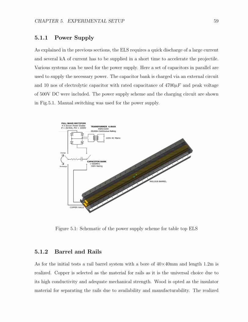
CHAPTER 5. EXPERIMENTAL SETUP 59
5.1.1 Power Supply
As explained in the previous sections, the ELS requires a quick discharge of a large current
and several kA of current has to be supplied in a short time to accelerate the projectile.
Various systems can be used for the power supply. Here a set of capacitors in parallel are
used to supply the necessary power. The capacitor bank is charged via an external circuit
and 10 nos of electrolytic capacitor with rated capacitance of 4700µF and peak voltage
of 500V DC were included. The power supply scheme and the charging circuit are shown
in Fig.5.1. Manual switching was used for the power supply.
Figure 5.1: Schematic of the power supply scheme for table top ELS
5.1.2 Barrel and Rails
As for the initial tests a rail barrel system with a bore of 40×40mm and length 1.2m is
realized. Copper is selected as the material for rails as it is the universal choice due to
its high conductivity and adequate mechanical strength. Wood is opted as the insulator
material for separating the rails due to availability and manufacturability. The realized
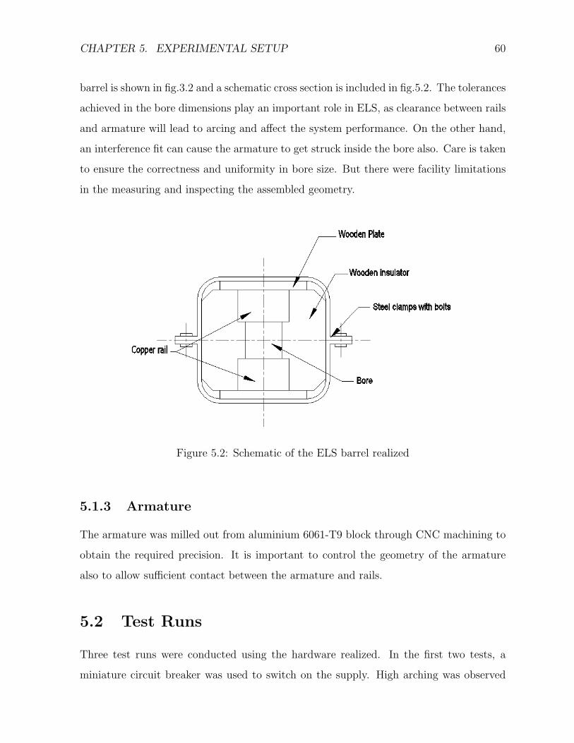
CHAPTER 5. EXPERIMENTAL SETUP 60
barrel is shown in fig.3.2 and a schematic cross section is included in fig.5.2. The tolerances
achieved in the bore dimensions play an important role in ELS, as clearance between rails
and armature will lead to arcing and affect the system performance. On the other hand,
an interference fit can cause the armature to get struck inside the bore also. Care is taken
to ensure the correctness and uniformity in bore size. But there were facility limitations
in the measuring and inspecting the assembled geometry.
Figure 5.2: Schematic of the ELS barrel realized
5.1.3 Armature
The armature was milled out from aluminium 6061-T9 block through CNC machining to
obtain the required precision. It is important to control the geometry of the armature
also to allow sufficient contact between the armature and rails.
5.2 Test Runs
Three test runs were conducted using the hardware realized. In the first two tests, a
miniature circuit breaker was used to switch on the supply. High arching was observed
CHAPTER 5. EXPERIMENTAL SETUP 61
and the armature was not ejected out. Later it is observed that the armature got spot
welded to the rails at the initial position.
In the third run, the switch was replaced with a 3 pole knife switch, which is again
a manually operated switch with high current rating. Very high arcing was observed at
the switch and the switch got damaged. This time also armature did not move from
initial position and spot welds were observed at the armature location during post test
inspection. The following are the possible causes of failure inferred from the tests
• A good share of the energy is wasted in arcing due to slow manual switching. The
solution is to use a faster switching circuit with the required current rating. A faster
switching circuitry is under development.
• The static friction between the rail and the armature might have blocked the ar-
mature from movement initially, which can lead to spot welding. The solution is to
use an injector to push in the armature in synchronization with the power supply
switching.
• The bore dimension were assembly dependant as per the design and needed precisely
machined components to keep the armature in contact with the rails. With the
realized hardware the tolerances achieved was not good and this also might have
resulted in fine gap between the armature and rails, which in turn can initiate arcing
and spot welding. An improvement over the system assembly is planned and the
realization is in progress.
5.3 ELS with Composite Housing
The total assembly is shown in Fig.5.3 and following are the major components of the
assembly.
Enclosure: The enclosure is in two piece, made of molded 10mm thick FRP and ribs
are provided to improve the structural integrity. Dovel-pins are included to guide during
assembly process.
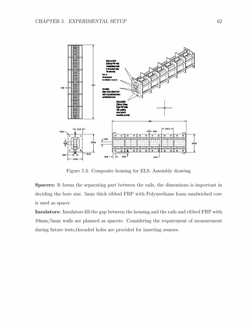
CHAPTER 5. EXPERIMENTAL SETUP 62
Figure 5.3: Composite housing for ELS: Assembly drawing
Spacers: It forms the separating part between the rails, the dimensions is important in
deciding the bore size. 5mm thick ribbed FRP with Polyurethane foam sandwiched core
is used as spacer
Insulators: Insulators fill the gap between the housing and the rails and ribbed FRP with
10mm/5mm walls are planned as spacers. Considering the requirement of measurement
during future tests,threaded holes are provided for inserting sensors.
Chapter 6
Conclusions and Future Scopes
An attempt has been made to simulate the ELS by modeling in the PDE module of the
COMSOLTM multi physics software. The simulation of electromagnetic interaction is
modeled using the potential form of Maxwell’s equations and the field distributions are
simulated. The forces coming on the armature and rails are also evaluated, which in turn
are used to predict the attainable velocity for the projectile. It is seen that the static
analysis is not sufficient to predict the forces and velocity. In the time dependant study,
the armature is assumed to be fixed at a particular location, which forms a quasi-steady
approximation of the problem. The forces and velocity are calculated for a linearly vary-
ing potential and for an exponential variation. The results shows a conservative estimate
of velocity up to 19km/s with an applied potential of 300V in 3ms for the exponentially
varying potential. Thus the possibility of using COMSOLTM for the simulation of electro-
magnetic phenomena is established and the same can be used for the design improvement,
once the other modules are added to the model for structural and thermal analysis.
An analytical study on the system dynamics is performed assuming Euler Bernoulli
theory with Lagrangian formulation to incorporate the frictional force due to the moving
armature. Characteristics of flexural and axial wave propagation is also studied and found
that the flexural wave propagation is predominant and all the four modes are present when
armature velocity in non-zero. Spectral finite element formulation is done to derive the
dynamic stiffness matrix as a function of frequency and the stability of the system is
63
CHAPTER 6. CONCLUSIONS AND FUTURE SCOPES 64
assessed for different frequency regimes. The study showed that the instabilities are more
for lower values of stiffness of structural containment and for higher armature velocities.
6.1 Scope for Future Work
This work was a preliminary estimate and the experimental validation of the results were
also aimed at, which could not be completed for want of time. Few initial runs test
runs tried out were not successful. So the next step shall be to validate the force and
acceleration levels from test results. In the simulation, applied potential characteristics
is assumed as an exponential discharge and the simulation can be repeated for appro-
priate power supply characteristics later, once the design is finalized. ELS basically is a
dynamic electro-mechanical system whose electromagnetic, structural and thermal prop-
erties are highly interdependent. To account for the coupled behavior, the model can be
extended with other modules for incorporating structural and thermal responses. The
system is modeled as a quasi-static one, with the armature position fixed with respect to
the rails and this is sufficient for a preliminary estimate. But for more detailed studies,
the possibility of incorporating armature movement in the model need to be explored.
In the laboratory experiments it was tried to propel a stationary armature, which can
probably be the reason to get it welded to the rail surface. Hence another module to
inject the armature in synchronization with the power switching may be added to over
come the problem associated with static friction. Extensive tests can be planned to assess
the system performance, effect of recoil etc. once the trial runs become successful.
Bibliography
[1] H.D.Fair, ”Electromagnetic Launch”, International J. of Impact Engineering., Vol.
29, pp. 246-262.
[2] Ian R. McNab, ”Minimization of the Input Power for a Long Railgun”, IEEE Trans.
on Magnetics Vol.39, No.1, Jan 1999
[3] D. E. Johnson et. al, ”The Efect of Rail Resistance on Railgun Efficiency”, IEEE
Trans. on Magnetics Vol.25, No.1, Jan 1989
[4] J. Mankowski et. al, ”A Bench Top Railgun With Distributed Energy Sources”, IEEE
Trans. on Magnetics, Vol.43, No.1, Jan 2007
[5] A. Sitzman et. al, ”Design, Construction, and Testing of an Induction Pulsed-Power
Supply for a small Railgun”, IEEE Trans. on Magnetics, Vol.43, No.1, Jan 2007
[6] F. Stefani,I. R. McNab et. al, ”A Plasma Railgun Experiment Addressing Launch-
to-Space Issues”, IEEE Transactions on Magnetics, Vol. 43, No. 1, Jan 2007
[7] DIANE Publishing, ”SDI: technology, survivability, and software”, ISBN:1428922679
[8] Ian R. McNab, ”JBIS -Electromagnetic Launch to Space” Vol.60, pp.54-62, 2007
[9] Ian R. McNab,”Launch to Space with an Electromagnetic Railgun” IEEE Trans. on
Magnetics, Vol.39, No.1, Jan 2003
[10] H. Kolm et. al, ”Electromagnetic propulsion alternatives”, AIAA-1979-1400
65
BIBLIOGRAPHY 66
[11] Onozuka M., Oda Y et. al, ”Railgun pellet injection system for fusion experimental
devices” Fusion Engg. and Design, Volume 30, Number 4, November 1995 , pp. 373-
383
[12] L. Tumonia,R. Kacianauskas, A.Kaceniauskas ”Evaluation of friction due to de-
formed behaviour of rail in the electromagnetic railgun: nemrical investigation” ISSN
1392-1207. MECHANIKA. 2007 Nr.1(63).
[13] D. R. Keefer, ”Boundary-Layer Efect on Railgun Muzzle Voltage”, IEEE Trans. on
Plasma Science, Vol.17, No.3, June 1989
[14] J. P. Barber, ”High Velocity Contact Properties”, IEEE Trans. on Magnetics,Vol.25,
No.1, Jan 1989
[15] H. A. Calvin,”The Development of Mega Ampere Contact Structures for an Electro-
magnetic Launcher”, IEEE Trans. on Components,hybrids, and Manufacturing Tech.
Vol.16, No.2, March 1993
[16] Lehmann, P., Peter, H., Wey J., ”Experimental study of solid armatures for EML
applications.” ,IEEE Trans.on Magn., 1993, No29(1), p.848-852.
[17] Urukov. B.A., Lebedev, A.D., Milyaev, C.C., ”Influence of materials properties on
the dynamics of metal armature acceleration in a railgun.”,-Proc. of the 4 European
Symposium on Electromagnetic Launch Technology, 1993, p.153-158
[18] Khandryga, D.V., Plekhanov, A.V, Tereschenko, A.N., ”Numerical simulation and
experimental results of the metal armature acceleration”, IEEE Trans. on Magn.,
1995, No31(1), p.193-197.
[19] P Lehmann, Minh Duc Vo, and Walter Wenning, ”Comparative Study of Rail-
gun Housings Made of Modern Fiber Wound Materials, Ceramic, or Insulated Steel
Plates”, IEEE Trans. Magn., Vol. 41, NO. 1, Jan 2005 pp 200-205
[20] H.D.Fair, ”Electric Launch Science and Technology in the United States” IEEE
Trans. Magn., Vol. 39, pp. 11-17, Jan. 2003.
BIBLIOGRAPHY 67
[21] Tzeng J, Zielinski A, Schmidt E, ”Design Considerations for Electromagnetic Rail-
guns” Journal of Pressure Vessel Technology 128 May 2006 pp 263-266
[22] Bauer. D.P,”Achieving high efficiency with conventional railgun launchers”, IEEE
Trans Magn., VOl.31 No. 1 Jan 1995
[23] Barber J. P, Bauer D.P et. al, ”A Survey of Armature Transition Mechanisms”, IEEE
Transactions on Magnaetics, Vol. 397, No. 1, January 2003, pp 47-51.
[24] G C Long, ”Railgun Current Density Distrbutions”, IEEE Transactions on Magnaet-
ics, Vol. 22, No. 6, November 1986.
[25] L. Rip, S. Satapathy, and K. T. Hsieh, Effect of geometry change on the current
density distribution in C-shaped armatures, IEEE Trans. Magn., vol. 39, pp. 72-75,
Jan. 2003.
[26] Asghar Keshtkar, ”Effect of Rail Dimension on Current Distribution and Inductive
Gradient”, IEEE Trans. on Magnetics Vol.41, No.1, Jan 2005.
[27] Ira Kohlberg et. al, ”A solution for the Three Dimensional Railgun Current Distri-
bution and Electromagnetic Fields of a Rail Launcher”, IEEE Trans. on Magnetics
Vol.31, No.1, Jan 1995
[28] J.T. Tzeng, ”Structural Mechanics for Electromagnetic Railguns”, IEEE Transac-
tions on Magnaetics, Vol. 41, No. 1, January 2005, pp 246-250.
[29] A. J. Johnson, F.C. Moon, ”Elastic Waves and Solid Armature Contact Pressure
in Electromagnetic Launchers”, IEEE Transactions on Magnaetics, Vol. 42, No. 3,
March 2006, pp 422-429.
[30] EMAS is the copyrighted product of McNed-Schwendler Corporation, USA.MEGA is
the copyrighted product of the University of Bath, UK. EMAP3D is the copyrighted
product of The University of Texas at Austin, USA.
[31] D. Rodger, T. Karaguler, and P. J. Leonard, ”A formulation for 3D moving conductor
eddy current problems”, IEEE Trans. Magn., vol. 25, pp. 4147-4149, Sept. 1989.
BIBLIOGRAPHY 68
[32] M. Ghassemi et. al, ”Analysis of Force Distribution Acting upon the Rails and the
Armature and Prediction of Velocity with Time in an Electromagnetic Launcher with
New Method”, IEEE Trans. on Magnetics, Vol.43, No.1, Jan 2007
[33] Marshall R A, Rashleigh S C, ”Electromagnetic acceleration of macroparticles to
high velocities”, J. Appl. Phy. Vol. 49(4) 1978, pp 2540-2542
[34] K. T. Hsieh, B. K. Kim, ”International Railgun Modeling Efort”, IEEE Trans. on
Magnetics Vol.33, No.1, Jan 1997
[35] W.F. Weldon et. al, ”Recoil in Electromagnetic Railguns”, IEEE Trans. on Magnet-
ics, Vol.Mag-22, No.6, Nov 1986
[36] David R. Saddin, ”Conservation of Momentum and Recoil in the Railgun”, IEEE
Trans. on Magnetics,Vol.33, No.1, Jan 97
[37] V G Endean, ”Forces on moving conductors and relativity”, J. Phys. D: Appl. Phys.
Vol. 22 (1989) pp 555-556.
[38] Peter Graneau, Neal Graneau, ”Electrodynamic force law controversy”,Phys. Rev. E
63, 058601 (2001)
[39] Peter Graneau, ”Amperian recoil and the efficiency of railguns”, J. Appl. Phys.
Vol.62, No. 7, October 1987
[40] Peter Graneau, ”Railgun recoil and relativity”,J. Phy. D: Appl. Phys. 20, 1987, pp
391-393
[41] Z. Castro-Dettmer, M. Simmons, and C. Persad, ”Obtainable microstructures in
electrical conductors made of a copper-silver alloy”, IEEE Trans. Magn., vol. 39, pp.
323326, Jan. 2003.
[42] B. M. Rech, R. C. Thompson, T. T. Pak, and G. A. Wedeking, ”Test methods
for composite structures for pulsed power rotating machines”, IEEE Trans. Magn.,
submitted for publication.
BIBLIOGRAPHY 69
[43] A. E. Zielinski, ”Thermophysical evaluation of a novel aluminum alloy with applica-
tion to an integrate launch package”, IEEE Trans. Magn. vol. 39, pp. 332336, Jan.
2003
[44] Gary L. Katulka et. al, ”Analysis of High-Temperature Materials for Application of
Electric Weapon Technology”, IEEE Trans. on Magnetics Vol.35, No.1, Jan 1999
[45] S. Rosenwasser and R. D. Stevenson, ”Selection and evaluation of insulator materials
for high performance railgun bores”, IEEE Trans. Magn., vol. 22, no. 6, pp. 17221729,
1986.
[46] D. Rodger, H. C. Lai, ”A Comparison of Formulations for 3D Finite Element Model-
ing of Electromagnetic Launchers”, IEEE Transactions on Magnaetics, Vol. 37, No.
1, January 2001.
[47] McNab IR, ”Early Electric Gun Research”, IEEE TRANSACTIONS ON MAGNET-
ICS, VOL 35, NO 1, JANUARY 1999.
[48] Barber J P Bauer D P, ”Hyper Velocity Railguns for Aeroballistic Testing” AlAA
92-3948, 17th Aerospace Ground Testing Conference Julv 6-8.1992
[49] F. Stefani and J. V. Parker, ”Experiments to measure gouging threshold velocity for
various metals against copper”, IEEE Trans. Magn., vol. 35, pp. 312316, Jan. 1999.
[50] F. Stefani and J. V. Parker, ”Experiments to measure wear in aluminum armatures”,
IEEE Trans. Magn., vol. 35, pp. 100-106, Jan. 1999.
[51] F. Stefani and R. Merrill, ”Experiments to measure melt-wave erosion in railgun
armatures”, IEEE Trans. Magn., vol. 39, pp. 188192, Jan. 2003.
[52] K. Zhang,D Li, ”Electromagnetic theory for microwaves and opto electronics”,
Springer 1998.
[53] Hsieh KT. ”A Lagrangian formulation for mechanically, thermally coupled electro-
magnetic diffusive processes with moving conductors”, IEEE Trans. Mag. Vol 31, No
1, 1995 pp604-609
BIBLIOGRAPHY 70
[54] A. J. Johnson, F.C. Moon, ”Elastic Waves in Electromagnetic Launchers”, IEEE
Transactions on Magnaetics, Vol. 43, No. 1, Jan 2007, pp 141-144.
[55] Doyle J F. ”Wave Propagation in Structures: Spectral Analysis Using Fast Discrete
Fourier Transforms”, - 2nd Ed.1997, Springer, ISBN 0-387-94940-2