MODELING AND ANALYSIS OF CUSTOMER REQUIREMENTS FROM A DRIVER’S SEAT

A THESIS SUBMITTED TO THE GRADUATE SCHOOL OF NATURAL AND APPLIED SCIENCES

OF MIDDLE EAST TECHNICAL UNIVERSITY

BY

VUSLAT ÇABUK

IN PARTIAL FULFILLMENT OF THE REQUIREMENTS

FOR THE DEGREE OF MASTER OF SCIENCE

IN INDUSTRIAL ENGINEERING

JANUARY 2008

ii

Approval of the thesis:

MODELING AND ANALYSIS OF CUSTOMER REQUIREMENTS FROM A DRIVER’S SEAT

submitted by VUSLAT ÇABUK in partial fulfillment of the requirements for the degree of Master of Science in Industrial Engineering Department, Middle East Technical University by, Prof. Dr. Canan ÖZGEN Dean, Graduate School of Natural and Applied Sciences _____________

Prof. Dr. Nur Evin ÖZDEMĐREL Head of Department, Industrial Engineering Department _____________

Prof. Dr. Gülser KÖKSAL Supervisor, Industrial Engineering Department, METU _____________

Examining Committee Members:

Prof. Dr. Nur Evin ÖZDEMĐREL Industrial Engineering Department, METU _____________________________

Prof. Dr. Gülser KÖKSAL Industrial Engineering Department, METU _____________________________

Assoc. Prof. Dr. Đnci BATMAZ Statistics Department, METU _____________________________

Assoc. Prof. Dr. Murat Caner TESTĐK Industrial Engineering Department, HU _____________________________

Dr. Ezgi DEMĐRTAŞ Industrial Engineering Department, EOU _____________________________

Date: 31.01.2008

iii

I hereby declare that all information in this document has been obtained and presented in accordance with academic rules and ethical conduct. I also declare that, as required by these rules and conduct, I have fully cited and referenced all materials and results that are not original to this work.

Name, Last Name: VUSLAT ÇABUK

Signature:

iv

ABSTRACT

MODELING AND ANALYSIS OF CUSTOMER REQUIREMENTS FROM A DRIVER’S SEAT

ÇABUK, Vuslat

M.S., Department of Industrial Engineering

Supervisor: Prof. Dr. Gülser Köksal

January 2008, 153 pages

In vehicles one of the most important components which affect comfort of the driver and

the purchasing decision is the driver’s seat. In order to improve design of a driver seat

in a leader company of automotive sector, a comprehensive analysis of customer

expectations from the driver seat is performed with a cross functional team formed by

representatives of design, marketing, production, quality and services departments. In

this study, collection of customer voice data and development of an exceptional

“customer satisfaction estimation model” using these data are presented. Data are

modeled by the help of Logistic Regression. This model is able to estimate how much a

v

given customer is likely to be satisfied with the driver seat at a certain confidence level.

It is also explained how this model can be used to identify design improvement

opportunities that help increase the probability that a customer likes the driver seat. The

modeling and analysis approach used for the particular case is applicable in general to

many other cases of product improvement or development.

Keywords: Voice of Customer, Logistic Regression, QFD, Driver seat

vi

ÖZ

BĐR SÜRÜCÜ KOLTUĞU ĐÇĐN MÜŞTERĐ ĐHTĐYAÇLARININ ANALĐZĐ VE MODELLENMESĐ

ÇABUK, Vuslat

Yüksek Lisans, Endüstri Mühendisliği Bölümü

Tez Yöneticisi: Prof. Dr. Gülser Köksal

Ocak 2008, 153 sayfa

Binek otomobillerde ve ticari araçlarda sürücünün konforunu ve alım kararını etkileyen

en önemli tasarım bileşenlerinden birisi sürücü koltuğudur. Otomotiv sektöründe faaliyet

gösteren bir firmada koltuğun tasarımını iyileştirmek için; tasarım, pazarlama, üretim,

kalite ve servis bölümlerinde çalışan kişilerden oluşturulan çapraz fonksiyonel bir ekiple

birlikte sürücü koltuğu için müşteri istek ve beklentilerinin kapsamlı bir analizi

gerçekleştirilmiştir. Bu çalışmada, müşterinin sesi verisinin toplanması ve bu verinin

alışılmışın dışında bir “müşteri beğenisi tahmin modeli”nin geliştirilmesinde kullanımı

sunulmaktadır. Veri Lojistik Regresyon yardımı ile modellenmektedir. Bu model verilen

vii

bir müşteri profili için koltuktan beğeniyi belirli bir güvenilirlikte tahmin

edebilmektedir. Çalışmada, aynı modelin, müşteri beğenisinin nasıl artırılabileceğinin,

dolayısıyla tasarımın nasıl iyileştirilmesi gerektiğinin belirlenmesinde kullanımı da

gösterilmektedir. Bu durum için kullanılan modelleme ve analiz yaklaşımı genel olarak

başka bir çok ürün geliştirme vakasında kullanılabilir.

Anahtar Kelimeler: Sürücü Koltuğu, Müşterinin Sesi, Lojistik Regresyon, Kalite

Fonksiyon Göçerimi (QFD)

viii

To my beloved parents Feyzullah & Ülzifet ÇABUK

ix

ACKNOWLEDGEMENTS

First of all I would like to give special thanks to my thesis supervisor, Prof. Dr. Gülser

Köksal for her professional support, trust, interest and patience during this study. She is

not only a supervisor for my thesis, but also a beloved guide for my life.

I would also like to give special thanks to Assoc. Prof. Dr. Đnci Batmaz for her pleasant

interest in every kind of my problems.

I would like to specify my thankfulness to my dear friend Elçin Kartal since she offers

me a lovely friendship, reliable support, and endless interest.

I would like to give thanks to TUBĐTAK for their internship and Huriye Karlı for her

trust. I owe also thanks for QFD team in TOFAŞ A.Ş., Dr. Ezgi Demirtaş, and Hasan

Karakaya for their aid.

I would like to express my gratitude to Kenan Bilirgen for his endless love. He always

supported me, makes me to feel in confidence, and helps me to overcome every kind of

difficulties. Thanks for his patience.

However most of all I have a great appreciation to my parents Ülzifet and Feyzullah

Çabuk for every think in my life. They always believed and supported me. Thanks for

their existence. I should also express my special thanks for my sister Dilara Çabuk. We

always encouraged us and shared everything in our lives.

x

TABLE OF CONTENTS

ABSTRACT.......................................................................................................................iv

ÖZ ......................................................................................................................................vi

ACKNOWLEDGEMENTS ...............................................................................................ix

TABLE OF CONTENTS....................................................................................................x

LIST OF TABLES .......................................................................................................... xiii

LIST OF FIGURES .........................................................................................................xiv

CHAPTERS 1 INTRODUCTION ..........................................................................................................1

2 LITERATURE SURVEY AND BACKGROUND ........................................................4

2.1 Quality Function Deployment and Voice of Customer Analysis ........................... 6

2.2 Logistic Regression............................................................................................... 15

2.3 Principle Component Analysis.............................................................................. 27

2.4 Factor Analysis ..................................................................................................... 28

2.5 Reliability and Validity of Surveys....................................................................... 31

3 MODELING AND ANALYSIS OF CUSTOMER REQUIREMENTS ......................37

3.1 The Approach........................................................................................................ 37

3.2 Data Collection...................................................................................................... 38

3.2.1 Customer Segments........................................................................................... 38

3.2.2 Sample Size and Stratified Sampling................................................................ 39

3.2.3 The Questionnaire ............................................................................................. 41

xi

3.2.4 Gemba Studies .................................................................................................. 42

3.3 Data Analysis ........................................................................................................ 43

3.3.1 Data Preprocessing............................................................................................ 43

3.3.2 Reliability and Validity of Data ........................................................................ 47

3.3.3 Simple Statistics ................................................................................................ 49

3.3.4 Factor Analysis ................................................................................................. 50

3.3.5 Models for Questions about Comfort................................................................ 61

3.3.6 Logistic Regression Analysis for Overall Satisfaction Grade........................... 62

3.4 Optimization and Prediction ................................................................................. 77

4 DISCUSSION ...............................................................................................................83

5 CONCLUSIONS AND FURTHER STUDIES ............................................................88

6 REFERENCES..............................................................................................................90

APPENDICES A CUSTOMER SEGMENTS TABLE (5W, 1H) (AN EXAMPLE) ..............................97

B THE QUESTIONNAIRE .............................................................................................98

C CUSTOMER PROFILES AND NUMBERS DETERMINED FOR GEMBA

STUDIES ........................................................................................................................109

D CUSTOMER (VOC) TABLE (AN EXAMPLE).......................................................110

E ITEM-TOTAL STATISTICS.....................................................................................111

F SOME SIMPLE GRAPHICAL ANALYSIS RESULTS ...........................................112

G CORRELATION MATRIX.......................................................................................114

H FACTOR ANALYSIS OUTPUT ..............................................................................117

I PRINCIPLE COMPONENT ANALYSIS OUTPUT..................................................120

xii

J SCATTER PLOTS OF THE PRINCIPLE COMPONENTS......................................121

K THE DECISION TREE MODEL ..............................................................................127

L LOGISTIC REGRESSION MODELS.......................................................................128

M EXPLANATION OF VARIABLES IN THE MODELS ..........................................132

N RESIDUAL PLOTS.................................................................................................1377

O VARIANCE ESTIMATION FOR THE DESIRED PROBABILITY.......................141

P CONFIDENCE INTERVAL ESTIMATION FOR �( )P Y j= ....................................145

Q OPTIMIZATION MODELS......................................................................................147

R INDIVIDUAL VALUE GRAPHS OF EACH MEASUREMENT ...........................151

xiii

LIST OF TABLES

TABLES

Table 1 Form of the Link Functions ................................................................................18 Table 2 Scale for the question 63 (overall satisfaction with the vehicle) ........................46 Table 3 Previous and new levels for overall satisfaction grade .......................................47 Table 4 Reliability statistics .............................................................................................48 Table 5 Statistics of the models with question 27 and without question 27 ....................66 Table 6 Selected anthropometrical variables and their loadings......................................67 Table 7 Statistics of the models .......................................................................................71 Table 8 Anthropometrical measures of a customer profile..............................................75 Table 9 Characteristics of the optimal profiles for Model 1 ............................................79 Table 10 Characteristics of the optimum profiles for Model 2........................................80

xiv

LIST OF FIGURES

FIGURES

Figure 1 Six Steps of QFD Process (Hsiao, 2002).............................................................9 Figure 2 Kano Model .......................................................................................................13 Figure 3 S Shape of the estimated values in Logistic Regression ...................................17 Figure 4 Box plot of variables belonging to weight.........................................................44 Figure 5 Box plots of variables belonging to anthropometrical measures (Questions 77-

89) ............................................................................................................................44 Figure 6 Pie Chart for the answers of question 63 ...........................................................46 Figure 7 Histogram of the differences between estimated probabilities of level 1 by the

two models ...............................................................................................................73

1

CHAPTER 1

INTRODUCTION

In vehicles one of the most important components which affect purchasing decision is

the driver seat. The driver seat is the interface between the vehicle and the driver. It

should provide accommodation, comfort and safety. The position of the driver seat

should not obstruct vision and reach of vehicle controls. It should be able to

accommodate driver having any size and shape, ensure comfort after a long drive and

provide a safe zone in a crash. Fore-aft (horizontal), vertical and back angle adjustments

are necessary to accommodate different body sizes and to supply constant vision.

Moreover stiffness, contour, climate, memory are some vehicle features that can

improve driver comfort. In addition a vehicle seat should absorb vibration (Peacock and

Karwowski, 1993; Shin et al., 2006; Makhsous et al., 2005).

Seat, which is in the correct driving body position, supplies dynamic sitting. In that

position back of the body and pelvis transmit body weigh to the seat. Thus arms and legs

can move freely, and head can be positioned for optimal vision and comfort. In addition

in the appropriate body position elbow, wrist, knee and ankle joints should be able to

move freely when it is needed. For safety of driver head restraint should be positioned

correctly (Peacock and Karwowski, 1993; Andreoni et al., 2002). In addition natural

2

spinal posture should be preserved in order to allow driver to change driving position

without disturbing his/her spine (Kolick, 2000).

There are three main parts of the driver seat. These are seat cushion, seat back and head

restraint. These main parts can be divided to some sub parts. For example cushion can be

divided as lateral wings, front, back and centre. Seat back can be divided as two lateral

wings, lower part, mid part and upper part (Verver et al., 2005). In addition arm restraint

can be added as fourth main part.

As it is seen, comfort on driver seat is related to body size. In order to improve

ergonomic design of the driver seat, anthropometrical measures of driver should be

taken into account. Especially body parts which are reclining to seat and used to reach

vehicle control should be measured. These are anthropometrical measures about weight,

length, heights while sitting and lengths while controlling vehicle. (Akın et al., 1998;

Çilingir, 1998)

Driver perception about a driver’s seat provides crucial information for the seat design.

In order to improve seat design, customer voice should be listened to. Quality Function

Deployment (QFD) is a very powerful tool to understand customer expectations and

ensure customer satisfaction. In the current study, a comprehensive analysis of voice of

the customer (VOC) about a driver’s seat is performed and a customer satisfaction

estimation model is constructed. Voice of the customer analysis approaches used as a

part of various QFD studies are presented in chapter 2. Our approach is similar to many

3

of those in data collection, but unique in analysis of the data to produce useful

information for the designers.

The modeling and analysis approach is explained in chapter3. The first step is data

collection (section 3.2). At this step a detailed questionnaire is prepared. Since

observations are made while customers are sitting on the seat, this questionnaire is a

kind of an observation plan. Number of customers to be visited is also determined. In

addition, target customer segments and their size in the sample are identified. After

collecting the data, they are analyzed (section 3.3). In this context, data preprocessing,

reliability and validity of data, and their factor analysis are discussed.

The relationship between customer satisfaction with the seat and many factors affecting

it is modeled by logistic regression. Use of such models to identify design improvement

opportunities is discussed. Another original study proposed and demonstrated in this

thesis is optimization of these models to find what kind of customers like (or dislike) the

driver seat the most (section 3.4). Such information can better help the designers

understand what are to be improved in the design.

4

CHAPTER 2

LITERATURE SURVEY AND BACKGROUND

One of the most important concerns of businesses is ‘to keep their competitive positions

in the marketplace’. Customer satisfaction is the key of competitiveness. Providing

quality product to customers can help achieve customer satisfaction. Whether the

product or service meets or exceeds expectations of customers should be the main aspect

of quality. In order to achieve it, the definition of “quality” should be cleared. As an

expression, it is used to express excellent product or service that exceeds the

expectations. There are different definitions of “quality”. According to ANSI/ASQC

standard A3-1987, “quality” is the totality of product or service features satisfying

implied and stated requirements. These requirements contain safety, availability,

maintainability, reliability, usability, price and environment (Besterfield et al. 1995).

Philip B. Crosby, who is one of the quality gurus, defined quality as conformance to

requirements, not as ‘goodness’ or ‘excellence’. The main idea of Crosby is built on zero

defects which mean ‘doing it the first time’ and ‘conformance to requirements’ (Flood,

1993). Juran, an early doyen of quality management, defined quality as ‘fitness for

purpose or use’. Deming expressed that quality should be aimed at the needs of

consumers, present and future. Feigenbaum explained ‘quality’ as the total composite of

product and service features of marketing, engineering, manufacturing and maintenance

5

through which the product and service in use will meet the expectations of customers

(Oakland and Marosszeky, 2006).

To summarize, quality which can be associated with many different environments

involves meeting and exceeding customer expectations. However, in traditional view,

businesses tend to see that productivity and quality are always in conflict. Total quality

management is a philosophy where lasting productivity gains are the results of quality

improvement. It emphasizes continuous improvement of product, processes and people

in order to prevent problems before they occur. It focuses on long-term profits and

continual improvement. In this view it is a function towards defects and it can be

measured and achieved. This philosophy needs comprehensive strategic plans that

contain vision, mission, and broad objectives. Customer focus, obsession with quality,

scientific approach, long term commitment, teamwork, continual process improvement,

education and training and freedom through control are the key elements of total quality

management approach (Goetsch and Davis, 2003).

According to these definitions quality is a term which is perceived by consumers and

measurable. Therefore products have characteristics describing their performance

relative to customer expectations. Especially in new product development processes

products should be measured in terms of quality characteristics. Total quality

management suggests that quality must be built into development process. By total

quality management approach problems can be prevented before they occur. If

6

development process is disciplined enough, it becomes predictable and faults become

preventable. In order to create a quality design in terms of aesthetics, efficiency,

manufacturing qualities and lower cost, some applications like concurrent engineering

(CE), quality function deployment (QFD), failure mode and effect analysis (FMEA),

design for assembly, design for manufacturability, statistical process controls (SPC),

analytical hierarchy process (AHP) should be integrated with new product development

in the total quality management umbrella (Hsiao, 2002).

2.1 Quality Function Deployment and Voice of Customer Analysis

QFD is the main tool for successful total quality management and product development

(Zairi and Youseff, 1995). It is a company wide solution to improve product design. It is

used to reduce cost and time of the design and to improve product quality by the help of

customer demands and communication between different functional areas (Pullman et

al., 2002). This centralizes QFD on customer satisfaction. It aims to improve customer

satisfaction with the quality of products or services (Mazur, 1996). By using QFD, cycle

time and engineering changes are reduced, startup cost is minimized, lead time is

shortened, customer satisfaction and market share are increased, warranty claims is

reduced, quality assurance planning becomes more stable and product returns are

decreased.

7

A design process includes product definition, design and redesign phases. In general

redesign phase is the result of insufficient knowledge about customer expectations. QFD

suggests spending enough time for definition and design steps. Eventually it diminishes

time spent for redesign. (King, 1989)

Starting evolution of QFD occurred in Japan between 1967 and 1972. Quality of design

and providing manufacturing with quality control charts before initial production are the

main drivers of the birth of QFD (Hill, 1994). Until 1972 Akao accomplished several

industrial trials. After that QFD was successfully used in many fields in Japan. By using

QFD, Toyota was able to reduce the costs of bringing a new car model to market by over

60% and to decrease the time required by one-third (Ullman, 1992). Then QFD moved

to US in 1980’s. Firstly, it was used in industries focused on automobiles, electronics,

and software. The fast development of QFD has resulted in its applications to many

manufacturing industries, and also in service sector such as government, banking and

accounting, health care, education and research. Some of the companies that used QFD

are 3M Company, Ford Motor, General Motors, Goodyear, IBM, Motorola, Procter and

Gamble, and Xerox. The main functional fields of QFD are product development, design

and planning, quality management, and customer needs analysis, decision-making,

engineering, management, teamwork, timing, and costing (Chan and Wu, 2002).

QFD is a process where firstly customer demands are collected and listed. Then

customer needs are converted into one or more finished product characteristics by the

8

help of house of quality (HOQ). After that, target values of the product characteristics

are tried to be determined by maximizing customer satisfaction and key product

characteristics are identified to be used in product design. At the end, design feature

targets, which meet the product characteristic targets and maximize customer

satisfaction, are identified. This procedure satisfies customer needs by saving time

(Pullman et al., 2002; Köksal and Smith, 1995).

QFD works with several activities examined by matrices. Besides matrix diagram,

affinity diagram, interrelationship digraph, tree diagram are the tools that can be used in

QFD projects (Goetsch and Davis, 2003; Cohen, 1995).

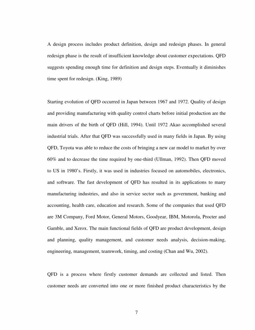
The basic idea in QFD is to translate voice of the customer (VOC) into technical

requirements. The procedures can be divided into six steps. These 6 steps are shown in

Figure, 1.

9

Figure 1 Six Steps of QFD Process (Hsiao, 2002)

Although QFD has been used for several decades it is still in a development. Recent

developments in QFD are focused on voice of customer analysis, determination of the

optimal technical targets, simplification and computerization of QFD process and the

use of artificial intelligence (Xie et al., 2003). US auto industry has modernized

traditional Japanese QFD since it is too large to control and time consuming to finish the

whole. It is also centralized on customer satisfaction but identification of minimum QFD

effort with desired results. This approach makes QFD more applicable for today’s lean

approach. Modern QFD based on Blitz QFD which decreases effort for QFD by

replacing the large matrix with a smaller one including only critical customer needs.

Moreover modern QFD is more statistically based and integrated with innovation

methods like TRIZ (QFD Institute, 2007).

Customer requirements Steps 1&2

Weighting functions Step 3

Requirement relations

Step 5b

Competition benchmarks Step 4

Engineering targets and benchmarks Step 6

Engineering requirements Step 5a

10

VOC is the input of QFD studies. Therefore, if it is misunderstood, whole QFD study

can be inaccurate. Customer voice should be identified, well understood and be carefully

stated, because VOC list should be complete and independent (Köksal and Smith, 1995).

In addition, how the product meets the customer demands, functions of the product that

customers may be aware or not, major sub-parts of the product should also be clearly

defined and deeply understood in order to continue QFD studies (King, 1989). There can

be more than one customer for a product supply chain. However end users are the most

important customers who put money into system. Therefore, if end users are satisfied

with the product, then everyone in the chain is content (Ronney et al., 2000). Customer

information can be divided into two parts: feedback and input. Feedback is the

information gathered after the fact and input is the information gathered before the fact.

Although feedback is valuable, input should also be collected, since it gives a chance to

change in product before producing, marketing and distributing it. These two kinds of

information can be categorized like solicited and unsolicited data. Both of the data can

be quantitative and qualitative (Goetsch and Davis, 2003). Collecting customer

information is used to discover customer dissatisfaction, their relative priorities of

quality, their needs and the opportunities for improvement. The main customer

information collection tools are comment cards, customer and market surveys, one-to-

one interviews, contextual inquires, focus groups, toll-free telephone lines and customer

visits. In addition, trade trials, working with preferred customers, analyzing products

from other manufacturers, registered customer complaints or lawsuits, independent

11

consultants, conventions, vendors, suppliers and employees are the sources where VOC

can be gathered (Besterfield et al., 1995; Cohen 1995). Another voice of customer

source which is suggested for QFD studies is going to GEMBA. As a literal definition,

GEMBA is the place where truth is known. This means to go to consumers and

observing their use of product to discover their expectations and opportunities to

improve (Rings et al., 1998). Unlike the traditional customer research that observe

consumers in an artificial place where they are asked questions about product without

seeing or using it, Gemba researches do not rely on customer memories and therefore

they are occurred in a natural place where customers use the product. Therefore this data

gathering method is using face to face observation method while taking advantage of

contextual inquiry, video tapping, audio tapping, direct observation and direct

interviewing with customers. It is better to have open ended question in questionnaire

applied in Gemba. Thus attaining to original customer statements is easy (Mazur, 1996).

During Gemba visits, surveyors collect the visual records about product usage, capture

customer problems and opportunity statements and discover competitive points of

product. In order to use information gathered in GEMBA original customer statements

should be recorded and then they should be restated in terms of opportunities for the

product improvement. In order to achieve generalized information, target customer

segments which can represent entire end users, and customer visit planning should be

constituted. In this guide, customer segments, time and place of the observations, type of

12

the information that is of interest and ways to gather information should be clarified

(Mazur, 1996; Ronney, 2000).

It is recommended that 10 or 12 Gemba visits are enough to gather information about

nearly 70% of customer requirements. Additional visits gives less new information

(Pouliot, 1992). In order to analyze customer statements, voice of the customer tables

can be used. Brainstorming, affinity diagram, hierarchy diagram, analytical hierarchy

process, customer segment table, check list, flow chart, customer process table, data

flow diagram, customer context table are examples of the other tools that can be used in

Gemba (Mazur, 1996).

However clarifying customer needs is not very simple. In general customers have

difficulties in expressing their expectations. Even they can easily say that they like or do

not like something, it can be difficult for them to explain why. Consumers may know

that there is a problem, but may not be able to explain how to solve it (Rings et al.,

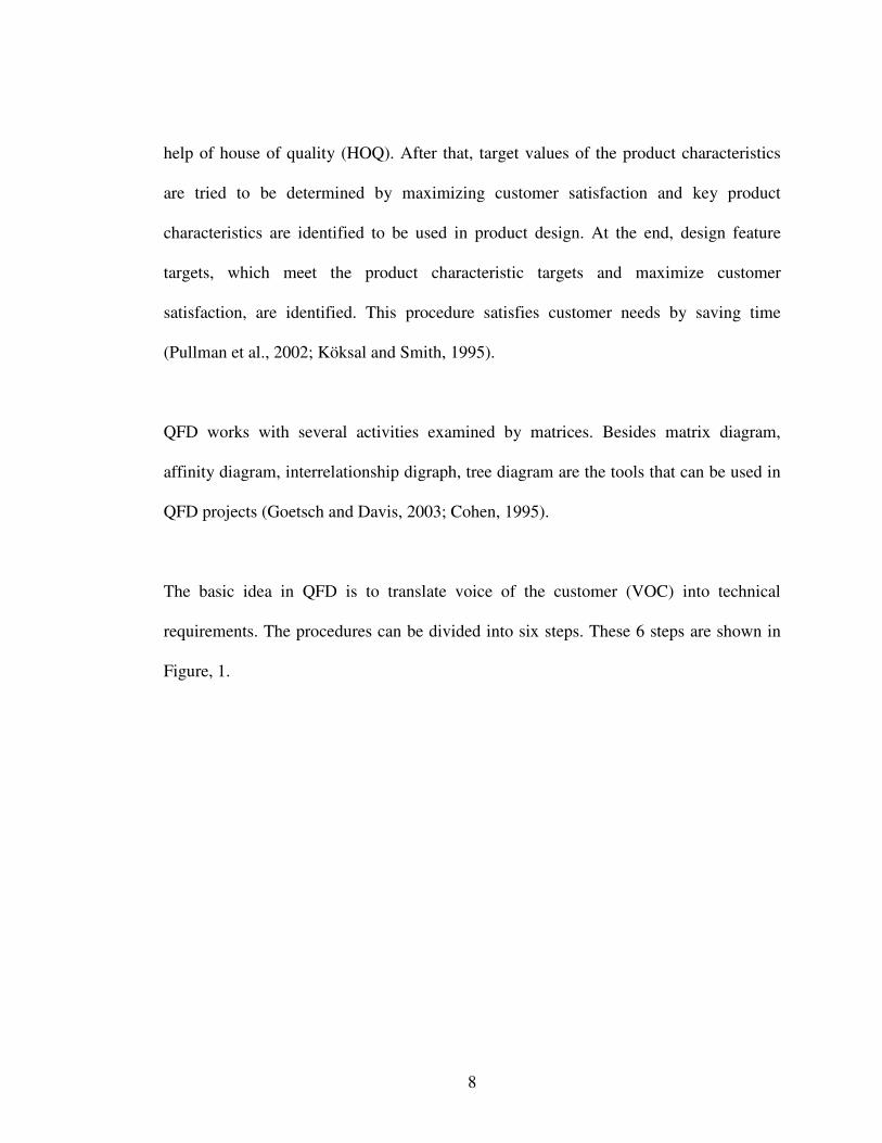
1998). Professor Kano categorizes quality attributes in three groups according to

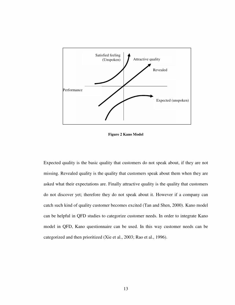
customer satisfaction: Attractive, revealed and expected (Tan and Shen, 2000). This

model approach can be used to collect efficient customer information. Kano’s chart

which explains relations between customer satisfaction and product performance is

shown in Figure 2.

13

Figure 2 Kano Model

Expected quality is the basic quality that customers do not speak about, if they are not

missing. Revealed quality is the quality that customers speak about them when they are

asked what their expectations are. Finally attractive quality is the quality that customers

do not discover yet; therefore they do not speak about it. However if a company can

catch such kind of quality customer becomes excited (Tan and Shen, 2000). Kano model

can be helpful in QFD studies to categorize customer needs. In order to integrate Kano

model in QFD, Kano questionnaire can be used. In this way customer needs can be

categorized and then prioritized (Xie et al., 2003; Rao et al., 1996).

Satisfied feeling (Unspoken) Attractive quality

Revealed

Expected (unspoken)

Performance

14

Prioritization of voice of the customer is another problem in HOQ process. Analytic

hierarchy process (AHP) and analytic network process (ANP) are multicriteria decision

making techniques that can be used to prioritize voice of the customer. Since

information gathered from people is based on their own backgrounds, it is possible to

have uncertainty in the data. Fuzzy group decision making techniques are suggested to

be applied in order to cope with this problem (Büyüközkan et al., 2004; Büyüközkan et

al., 2007). In addition, utility model or score model can be used instead of subjective

judgments. Some of the recent studies about how to prioritize VOC focus on changes on

customer expectation by the time. According to these studies, it is not enough to be

aware of the current VOC since it can change in the future. Therefore there is a

possibility that the results obtained from QFD analysis based on the current VOC cannot

meet customer requirements in the future. In order to solve this problem, in addition to

the current expectations of ordinary customers, future expectations of the lead users can

be collected. Then these two types of information can be integrated. In general, to collect

future expectations is not practical, since customers may not be aware of the

technological changes that can occur in the future. Forecasting techniques can be

alternative to forecast future prioritization of customer voices where researcher has

sufficient historical data. However, since the expectations of customers change rapidly,

although historical data is collected some new requirements can be added to the

customer voices. In this situation these new customer voices do not have historical

information. Moreover, in the companies which have just started to apply QFD, it is

almost impossible to find historical data. When there is not sufficient historical data

15

fuzzy trend analysis can be applied (Xie et al., 2003). All of the methods mentioned

above are based on asking to customers to prioritize their requirements. Instead of

customer prioritization methods, statistical methods can be used to analyze qualitative

voice of customer like their preferences or agreements with a statement. These kinds of

studies deal with also variability in VOC. Logistic regression can be applied to model

customer satisfaction and their preferences. In addition, by the help of demographic data,

satisfaction of different customer segments can be estimated based on statistical

significance (Lawson and Montgomery, 2006). In this study logistic regression is used to

model customer satisfaction probability and to obtain profiles of customers who like (or

dislike) the driver’s seat the most.

2.2 Logistic Regression

Even though linear regression is routinely used in manufacturing process improvements,

it is not useful in many business processes since most of them have binary, nominal or

ordinal outputs. Customer satisfaction is an example for qualitative output which

businesses may want to optimize. Lawson and Montgomery (2006) suggest Logistic

Regression Model to analyze customer satisfaction data. Logistic regression model is a

method to examine relationship between a qualitative response variable and one or more

explanatory variables. Response variable in logistic regression can be binary, nominal or

ordinal. Artificial Neural Network (ANN), Multivariate Adaptive Regression Splines

16

(MARS), and Decision Tree Models (DT) can be also used to analyze this kind of data.

ANNs are the collection of artificial neurons which are the collection of a large number

of single units (Fu, 1994). The strength of each connection is presented with weights

which are adjusted by learning phase. Neurons use a mathematical or computational

model to produce an output. There are three parts of ANN: input layer, hidden layers,

and output layer. MARS is an adaptive procedure to handle with high dimensional

regression problems (Friedman, 1991). It builds a flexible models by fitting piecewise

linear regression models. DT uses tree shaped structure to make classification. By using

tree shape, data is split into subgroups and the leaf nodes represent classes. In this study

Logistic Regression is selected to analyze data since, it provides probabilistic statements

by the help of a mathematical model while classifying the response. In addition there is a

possibility to build a significant confidence interval for the estimated probability.

Moreover optimization can be applied to the obtained model to see improvement

opportunities for the product design.

In binary logistic regression, response variable has two levels 0 or 1. Yes/ No questions

are the example for them. The difference between linear regression and logistic

regression is that linear regression estimates expected value of Y given the values of X,

(E(Y|X)), however logistic regression estimates probability of an event occurs given the

values X, (P(Y=1|X)).

17

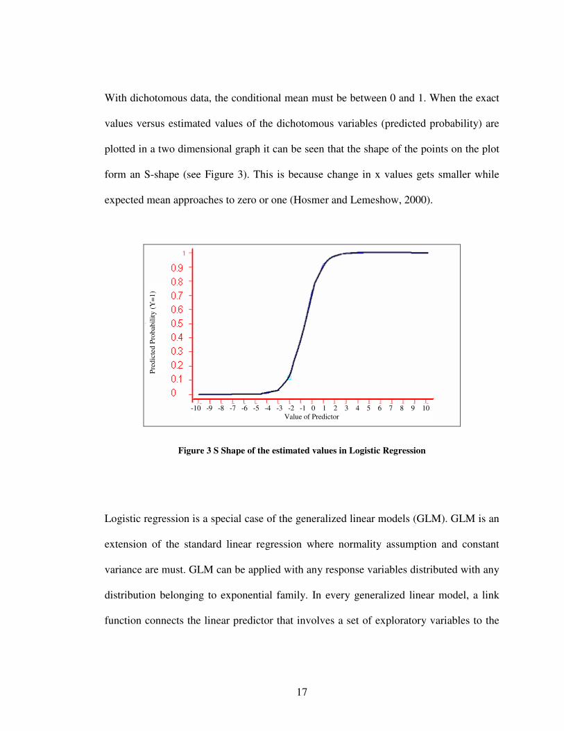
With dichotomous data, the conditional mean must be between 0 and 1. When the exact

values versus estimated values of the dichotomous variables (predicted probability) are

plotted in a two dimensional graph it can be seen that the shape of the points on the plot

form an S-shape (see Figure 3). This is because change in x values gets smaller while

expected mean approaches to zero or one (Hosmer and Lemeshow, 2000).

Figure 3 S Shape of the estimated values in Logistic Regression

Logistic regression is a special case of the generalized linear models (GLM). GLM is an

extension of the standard linear regression where normality assumption and constant

variance are must. GLM can be applied with any response variables distributed with any

distribution belonging to exponential family. In every generalized linear model, a link

function connects the linear predictor that involves a set of exploratory variables to the

-10 -9 -8 -7 -6 -5 -4 -3 -2 -1 0 1 2 3 4 5 6 7 8 9 10 Value of Predictor

Pre

dict

ed P

roba

bili

ty (

Y=

1)

18

response variable which is distributed from an exponential family (Lawson and

Montgomery, 2006). In logistic regression there are three link functions called logit,

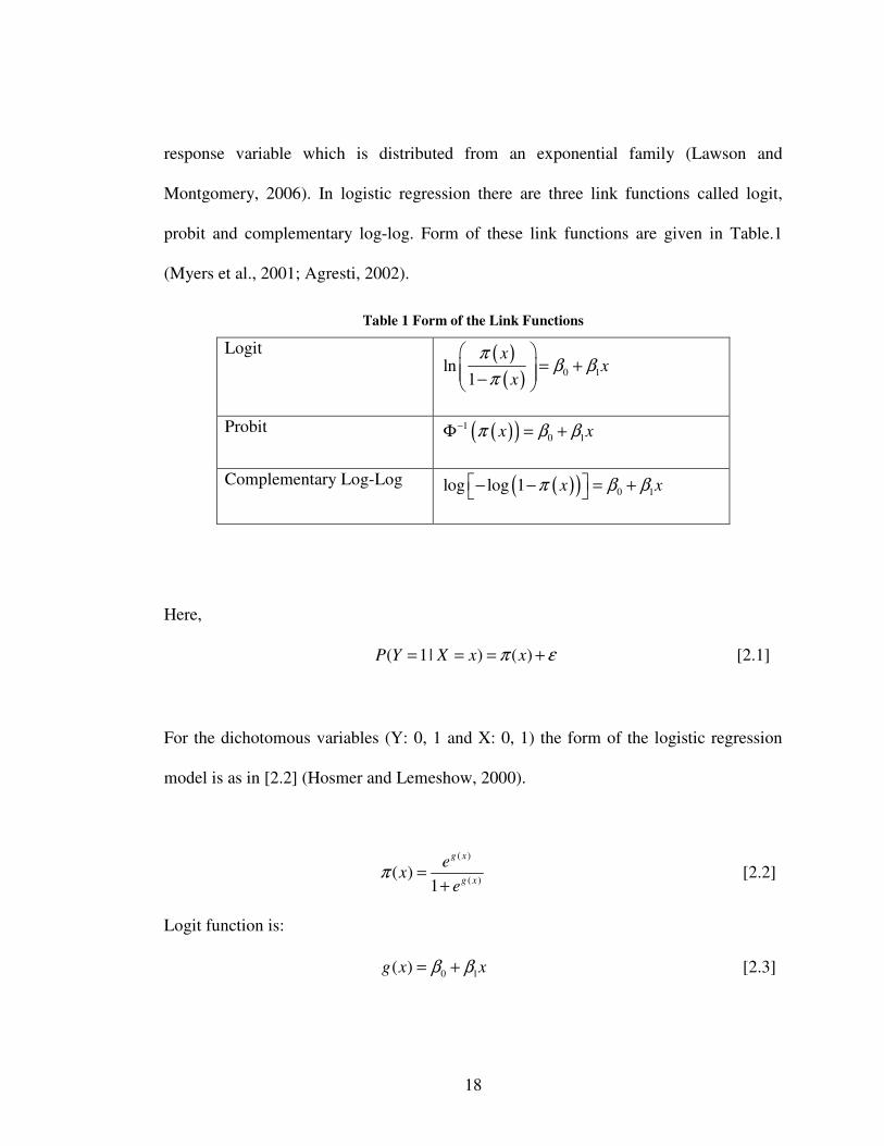
probit and complementary log-log. Form of these link functions are given in Table.1

(Myers et al., 2001; Agresti, 2002).

Table 1 Form of the Link Functions

Logit ( )( ) 0 1ln

1

xx

x

πβ β

π

= + −

Probit ( )( )10 1x xπ β β−Φ = +

Complementary Log-Log ( )( ) 0 1log log 1 x xπ β β − − = +

Here,

( 1| ) ( )P Y X x xπ ε= = = + [2.1]

For the dichotomous variables (Y: 0, 1 and X: 0, 1) the form of the logistic regression

model is as in [2.2] (Hosmer and Lemeshow, 2000).

( )

( )( )

1

g x

g x

ex

eπ =

+ [2.2]

Logit function is:

0 1( )g x xβ β= + [2.3]

19

( )ˆ( ) ( 1| )ˆ1 ( ) ( 0 | )

g x x P Y xe

x P Y x

π

π

== =

− = [2.4]

( 1)ˆ( 1| 1)ˆ( 0 | 1)

g x P Y xe

P Y x

= = ==

= = [2.5]

( 0)ˆ( 1| 0)ˆ( 0 | 0)

g x P Y xe

P Y x

= = ==

= = [2.6]

0 11

0

( 1)

( 0)

ˆ ˆ( 1| 1) ( 1| 0)ˆ ˆ( 0 | 1) ( 0 | 0)

g x

g x

P Y x P Y xe e ee eP Y x P Y x

β β ββ

+=

=

= = = == = =

= = = = [2.7]

In the formula [2.7] 1eβ is the Odds Ratio, Y=1 is the event and x=0 is the reference

value for the predictor.

Significance of the coefficients

If model with a variable is more accurately representing observed values than the model

without the variable, this variable should be in the model. Test of significance of a

variable is the comparison of the saturated model (that contains as many parameters as

there are in the data) and fitted model with and without variable. This method uses

likelihood ratio test approach.

The comparison of observed and predicted values (Hosmer and Lemeshow, 2000):

20

� ( )( )

� ( )1

likelihood of fitted model2 ln

likelihood of saturated model

12 ln 1 ln

1

ni i

i i

i i i

D

x xD y y

y y

π π

=

= −

− = − + −

− ∑

[2.8]

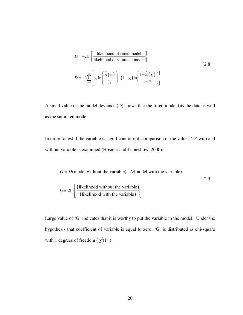
A small value of the model deviance (D) shows that the fitted model fits the data as well

as the saturated model.

In order to test if the variable is significant or not, comparison of the values ‘D’ with and

without variable is examined (Hosmer and Lemeshow, 2000):

( )( )

(model without the variable) - (model with the variable)

likelihood without the variableG=-2ln

likelihood with the variable

G D D=

[2.9]

Large value of ‘G’ indicates that it is worthy to put the variable in the model. Under the

hypothesis that coefficient of variable is equal to zero, ‘G’ is distributed as chi-square

with 1 degrees of freedom ( χ2(1) ) .

21

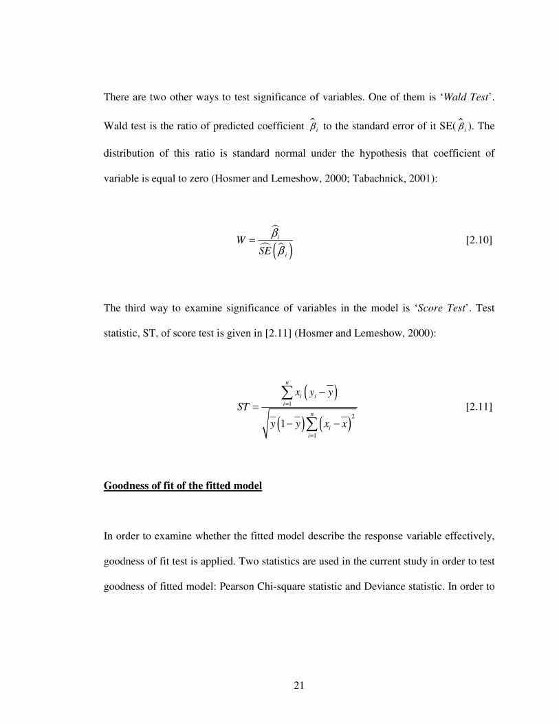
There are two other ways to test significance of variables. One of them is ‘Wald Test’.

Wald test is the ratio of predicted coefficient ɵ iβ to the standard error of it SE( ɵ iβ ). The

distribution of this ratio is standard normal under the hypothesis that coefficient of

variable is equal to zero (Hosmer and Lemeshow, 2000; Tabachnick, 2001):

�

� �( )i

i

WSE

β

β= [2.10]

The third way to examine significance of variables in the model is ‘Score Test’. Test

statistic, ST, of score test is given in [2.11] (Hosmer and Lemeshow, 2000):

( )

( ) ( )1

2

1

1

n

i i

i

n

i

i

x y y

ST

y y x x

=

=

−

=

− −

∑

∑ [2.11]

Goodness of fit of the fitted model

In order to examine whether the fitted model describe the response variable effectively,

goodness of fit test is applied. Two statistics are used in the current study in order to test

goodness of fitted model: Pearson Chi-square statistic and Deviance statistic. In order to

22

examine goodness of fit, residuals (differences between observed and fitted values) of

the model are used (Hosmer and Lemeshow, 2000).

Pearson residual

�( )�( )

� �( ),

1

ii

ii

i i

yr y

ππ

π π

−=

−

[2.12]

Under the hypothesis that the model is correct

�( ) ( )2

1

, ~ 1I

ii

i

r y I pπ χ=

− −∑ [2.13]

In [2.13] ‘I’ is number of parameters in saturated model and ‘p+1’ is the number of

parameters in the fitted model.

Deviance residual

�

�( )

�

12

1( , ) 2 ln 1 ln

1i i

ii i i

i i

y yd y y yπ

π π

− = ± + −

− [2.14]

Under the hypothesis that the model is correct

� ( )2 2

1

( , ) ~ 1I

ii

i

d y I pπ χ=

− −∑ [2.15]

23

In [2.15] ‘I’ is number of parameters in saturated model and ‘p+1’ is the number of

parameters in the fitted model.

In ordinary linear regression R2 values are used to find out proportion of variance

explained by the model. This value is the ratio of the regression sum of squares,

SSregression, to the total sum of squares, SStotal (Tabachnick, 2001).

2 regressiontotal residualOLR

total total

SSSS SSR

SS SS

−= = [2.16]

In logistic regression an analogy of this measure can be obtained by using deviance

between predicted model and model with only intercept (no other variables) (Hosmer

and Lemeshow, 2000).

2 0L

0

PL L

RL

−= [2.17]

In [2.17] ‘L0’ is the log likelihood of model with only intercept; ‘Lp’ is the log likelihood

of model with p covariates.

There are three modified versions of this basic idea, Mc Fadden R2, Cox & Snell

Pseudo-R2,, Nagelkerke Pseudo-R2 (Tabachnick, 2001).

24

Mc Fadden’s R square: This R2 is a transformation of likelihood ratio statistics within a

range of (0, 1).

2

0

1 p

McFadden

LR

L= − [2.18]

In general McFadden’s R2 tends to be much lower than R2 for multiple regressions.

Cox & Snell Pseudo-R2: This R2 is a version of r-square based log likelihood.

( )2Cox & Snell 0

21 exp pR L L

n

= − − −

[2.19]

The problem in this R2 is that it cannot reach 1.

Nagelkerke Pseudo-R2: This R2 is the modification of Cox&Snell Pseudo R2 in order to

make it to be able to reach 1.

22 Cox & Snell Nagelkerke 2

MAX

RR

R= [2.20]

where

( )2 1MAX 01 exp 2R n L

− = − [2.21]

In general R2 values in logistic regression are low when compared to the ordinary linear

regression R2 values. In addition, even goodness of fit statistics show that the model fit

25

well, R2 values of the model can be small. Therefore, in logistic regression, R2 values are

not recommended to use while deciding how a model fits the data. However they can be

used while comparing two or more alternative models (Hosmer and Lemeshow, 2000).

Strategies to select variables

A strategy should be used to select variables in the model when there are many variables

in data. Stepwise procedure is one of the widely used procedures in logistic regression

while selecting variables. In each step of stepwise procedure the variable that causes

greatest increase in ‘G’ statistic is selected to enter to the model. An alpha level should

be decided in order to judge the importance of a variable. This is the entrance alpha (PE)

which also determines when the procedure should stop. After entering a variable to the

model there is a possibility that one of the old variables becomes unnecessary in the

model and with backward elimination it is removed from the model. An alpha value for

backward elimination (PR) should be defined in order to decide whether a variable is

unnecessary in the model or not. Then the procedure continues until any of the

remaining variables cannot add significant information to the model.

Numerical Problems in Logistic Regression

Zero cell: When a level of the independent variable does not have at least one levels of

the dependent variable, ‘zero cell problem’ occurs. This causes division by zero while

computing odds ratio (OR). Therefore logistic regression algorithm does not work. This

problem can be detected by a large estimated coefficient and especially large estimated

26

standard errors. In order to eliminate this problem, discrete variables which have ordered

scale can be treated as continuous variables, levels of variables that have zero cells can

be collapsed or if collapsing can not be applied these variables can be removed from the

analysis (Hosmer and Lemeshow, 2000).

Complete and quasi-complete separation: This problem occurs when a collection of the

covariates separates (discriminate perfectly) the outcome groups. For example if whole

females in the data satisfied with the seat and whole males dissatisfied then complete

separation would be occur. This type of the problem depends on the sample size. The

risk of having complete separation is increasing while the difference between the

frequencies of the levels of dependent variable is increasing (Hosmer and Lemeshow,

2000). This problem can also be detected by a large estimated coefficient and especially

large estimated standard errors. In order not to have this problem in the analysis, the

main effects which can cause complete separation in the model can be removed from the

analysis. Using hierarchical structure for the interactions in the model increases

complete separation problem risk in the model.

Multi Collinearity between variables: While working with a complex data set, in order

not to have multi collinearity problems, it is better to examine correlations between

variables before analyzing them. Correlation matrix is a symmetrical matrix where each

element represents correlation between two variables. Matrix results are indicators of the

27

relationship among variables (Tabachnick, 2001). There are two main data reduction

methods using correlation matrix: Principle component analysis and Factor analysis

2.3 Principle Component Analysis

Principle component analysis (PCA) is a technique used to form new uncorrelated

variables which are linear composites of original variables. By PCA method a new

orthogonal variable set which includes most of the information of the data is

constructed. These new variables are principle component scores where the first variable

accounts for the maximum variance; the second variable has the maximum variance that

is not accounted by the first variable and so on. Assuming that there are p original

variables the algebraic form of principle components is given in [2.22] (Sharma, 1996).

1 11 1 12 2 1

2 21 1 22 2 2

1 1 2 2

.

...

...

.

...

p p

p p

p p p pp p

w x w x w x

w x w x w x

w x w x w x

ε

ε

ε

= + + +

= + + +

= + + +

[2.22]

In [2.22] ‘ 1,.....,p

ε ε ’ are principle components, ‘wij’ is the weight of jth variable for the

ith principle component.

1 2

2 2 2... 1 i=1,...,pi i ip

w w w+ + + = [2.23]

28

1 1 2 2... 0 for all i j

i j i j ip jpw w w w w w+ + + = ≠ [2.24]

Principle components analysis can be performed on either standardized or mean

corrected data. One of the most important issues in principle components analysis is to

decide on the number of components. If standardized data are used, the components

whose eigenvalues are greater than one can retain. This rule is named ‘eigenvalue-

greater-than-one’ (Sharma, 1996).

2.4 Factor Analysis

Factor analysis is an interdependence method to find out the structure of interrelations

between variables. It is used to collect information from number of variables in a smaller

set without loosing remarkable information. Factor analysis gives two different kinds of

information to a researcher. These are data summarization and data reduction. There are

two types of factor analysis: R-factor analysis which summarizes variables and Q-factor

analysis which summarizes observations. Since it provides smaller new data sets, it can

be seen as starting point for the other multivariate techniques.

The starting point of factor analysis is correlation matrix. If there is no substantial

number of correlations greater than 0.30, then it is not appropriate to apply factor

29

analysis. With the factors, at least 60% of the total variance should be accounted. This

can be used while deciding on the required number of factors (Hair et al., 2005).

Loadings in the factor matrix give considerable information. Factor loadings are

correlations between variables and factors. Higher loadings make variables

representative of factor. In this sense loadings are indicators of whether a variable is

significant for a factor or not. Loadings between ± 0.3 and ± 0.4 are minimal levels to

accept, loadings greater then ±0.5 are partially significant and loadings exciding ±0.7

can be seen as indicator of well defined structure. Moreover in order to say that a

variable has a sufficient explanation by the factors, its communality should be at least

0.50 (Hair et al., 2005).

Rotations can be used to obtain simple and theoretically more meaningful factors by

redistributing variances. Orthogonal factor rotation methods are most useful rotation

methods. Some of them are Varimax, Quartimax and Equimax.

Sample size of the data where factor analysis is applied becomes very important. Larger

sample size decreases standard errors in factor loadings. Thus factor loadings become

more precise. In the literature there are several studies on the required sample size in

factor analysis. These studies mostly focus on sample size, N and the ratio of N to the

number of variables being analyzed, p. The studies focused on just sample size

recommend diverse and contradictory sample sizes. Suggested sample sizes change from

30

50 to 250 (Hair et al., 2005; MacCallum and Widaman 1999; Guadagnoli and Velicer,

1988). Some studies are focused on N:p ratio. Pennell (1968) finds that while

communalities of variables are increasing, effect of sample size on factor loadings is

decreasing. There are also diverse recommendations on it. Hair et al. (2005) suggest N:p

ratio as 5.0. Whereas Barret and Kleine (1981) obtain efficient results with N:p ratios 1.2

and 3.0. Arrindell and van der Ende (1985) find that for 76-item questionnaire N=100 is

sufficient and for 20-item questionnaire N=78 is sufficient. These correspond to N:p=1.3

and 3.9, respectively. MacCallum and Widaman (1999) find that as N increases,

sampling error will be reduced and that’s why factor analysis results will be more

accurate. At the same time, quality of factor analysis results is increasing while

communalities are increasing, and this decreases the effect of sample size on the results.

After statistically significant factors are determined, discussing their appropriateness and

interpreting and labeling them are in the researcher’s judgment. There are two ways to

use information gathered by factor analyses in the further multivariate analysis. One of

them is to use the variable having highest loading in the factor as a surrogate

representative of the factor. The second way is to use summated scale instead of

variables.

31

2.5 Reliability and Validity of Surveys

If the questionnaire has scaled additive answers, it is better to discuss its reliability and

validity before analyses. In order to answer the question whether the questionnaire

measures customer satisfaction in a useful way or not, reliability of scales should be

investigated. Scales are reliable if they consist of items sharing common latent variable.

There are four strategies to analyze reliability of a scale: test-retest, alternate forms,

split-half, internal consistency (Murphy and Davidshofer, 1998). Test-retest method is

the oldest method which is based on applying the same test to the same group two times

in a period. After applying the second test, correlation between scores on the first test

and the scores on the second test is calculated to estimate reliability. Since there is a time

between two tests, it is possible that differences between scores can occur because of the

change in the participants’ decisions by the time. Besides this, to apply the same test as a

second time may channel participants to be reactive, since they already experienced the

same test before. Alternate form methods, on the other hand, is a way to solve some

negative effects of the test-retest method by applying two different but parallel tests to

the same participants in a period. However, since the tests are not the same, there is no

need to have a long time between them. This prevents the participant to be reactive and

at the same time the participant does not have enough time to change his/her decision

over the time. On the other hand, both of these methods are time consuming and

expensive, since they are applied two times. Split half method is a way to minimize the

32

negative effect of test-retest and alternate form methods. It is based on applying a test to

participants and then splitting the test in half. Correlation between scores of the first half

to the second half estimates reliability. Split half method can solve problems about

reactivity and change over time. In addition since only one test is applied, it is not time

consuming and expensive like the others. The problem in split half method is about how

to split the test. There can be differences in correlation of the two halves obtained by

different split types. Then it is difficult to decide which split half reliability estimate to

use. Therefore result of this method is also about order of the items in test. Finally,

internal consistency estimates reliability of a test based on merely a correlation among

test items and number of items. This takes into account different items’ variances. The

difference between split half method and internal consistency method is that split half

compares one half of the test to the other whereas internal consistency compares each

item of the test to every other item (Murphy and Davidshofer , 1998; Özdamar, 1997).

Coefficient alpha (Cronbach’s alpha) is an internal consistency way to estimate

reliability of scales. It is a value expressing internal consistency of items while

computing the proportion of scale’s total variance that is attributable to common source.

Cronbach’s alpha calculation is based on variance covariance matrix. Variance

covariance matrix of a data set having tree items for a latent variable is given in [2.25]:

21 12 13

221 2 23

231 32 3

σ σ σ

σ σ σ

σ σ σ

Σ =

[2.25]

33

In [2.25]:

2i

σ = variance of ith item

ijσ = covariance between ith and jth items

Common variability is the total of elements out of the diagonal in the matrix and total

variability is the total of all elements in the matrix.

( )2

1

i

x

x xs

n

Σ −=

− [2.26]

Equation [2.26] is the sample standard deviation of the item x

( )( )1

i i

xy

x x y ys

n

Σ − −=

− [2.27]

Equation [2.27] is the covariance between items x and y

Coefficient alpha is calculated based on the ratio of the common variability to the whole

variability (DeVellis, 2003; Thompson, 2003):

34

2

21

1

k

Total

k

k

σ

ασ

= −

−

∑ [2.28]

In the equation [2.28],

k: number of items

2i

σ : Variance of the answers belonging to ith question

2Total

σ : Total variance

2 2 2Total k ij

σ σ α = + ∗ ∑ ∑ (for i < j) [2.29]

For the data with tree items for a latent variable, Cronbach’s alpha is:

( )12 13 23

2

2 * *

1 Total

k

k

σ σ σα

σ

= −

[2.30]

In order to have reliable data, most of the variability of the items should be common.

That means that covariance between variables should be near to total variance and it is

better to have small item variance which decreases also covariance.

35

The Kuder-Richardson formula 20 (KR-20) is a special version of alpha for

dichotomous variables. These variables are answers where the participant is forced to

accept or refuse the statement. KR-20 estimate is computed as given in [2.31]

(Thompson, 2003):

220 1

1

k k

Total

p qk

KRk σ

− = −

−

∑ [2.31]

where

k: number of items

pk: proportion of people with a score 1 on the kth item

qk: proportion of people with a score 0 on the kth item

2Total

σ : Total variance

Coefficient alpha is a value between 0 and 1. The following rule can be used to decide

whether the scale is reliable or not: (Özdamar, 1997)

• 0.00 ≤α< 0.40 � scale is not reliable

• 0.40 ≤α< 0.60 � reliability is low

36

• 0.60 ≤α< 0.80 � scale is reliable

• 0.80 ≤α< 1.0 � scale is highly reliable

A reliable scale does not guarantee that the latent variable is the variable that is

concerned by the researcher. Validity is the concept which concerns whether the scale

scores represent characteristics of true score. This is the issue to deal with during

construction of the scale. Ability to predict specific events and relationships between

constructs should be considered. While concerning about validity some important points

should be kept in mind. Firstly selected items should represent a content domain. While

using measures of attributes to ensure that the items represent a content domain is very

difficult. Another important point to achieve validity is to access empirical association

between scale and some criteria. Here theoretical proof of association is not necessary

(DeVellis, 2003).

37

CHAPTER 3

MODELING AND ANALYSIS OF CUSTOMER REQUIREMENTS

3.1 The Approach

Companies such as automobile producers would like to reach their customers,

understand their expectations and identify opportunities to improve their products and

parts such as the driver’s seat, accordingly. In general, customers have difficulty in

explaining why they like or dislike a product. The approach we propose and demonstrate

in this thesis to understand, model and analyze customer requirements can be briefly

explained as follows: First, target customer segments are determined, and after that

Gemba visits are performed. During these visits firstly clients are observed freely using

the product. Then a detailed questionnaire is applied. The questionnaire includes

questions about the customer’s personal identification, and comfort, usage and

appearance of the driver seat. Also, anthropometrical measures of the customers are

recorded. In order to model voice of the customer (VOC) in an effective way,

anthropometrical data and answers to the questions are analyzed by the help of Logistic

Regression. Before logistic regression modeling, data are processed for missing values,

outliers, inconsistent values, and a factor analysis is applied to understand correlations

between answers, and principle component analysis is applied to identify linearly

38

independent components of correlated data. The logistic regression model estimates

probability of satisfaction with the driver seat for a given customer profile. We propose

to optimize such models to identify how the product design can be improved to increase

the satisfaction probability.

In this thesis, we use the modeling and analysis approach described above for driver seat

of a light commercial vehicle produced in Turkey.

3.2 Data Collection

3.2.1 Customer Segments

First of all, different customer groups, who use the vehicle for different purposes, are

analyzed. In order to identify customer segments, QFD team members get together and

fill the customer segment table (4W 1H). An example for a customer segment table (4W

1H) is shown in Appendix A. This table consists of five columns which are who, when,

where, why and how. In the column called as ‘who’ the different kinds of persons who

are the potential customers of the vehicle are listed. In the column called as ‘when’ the

possible times when the customers use the product (driver’s seat) are listed. In the

column called as ‘where’ the possible places where the customers use the product are

listed. In the column called as ‘why’ the possible reasons why the customers use the

vehicle are listed. Lastly, in the column named as ‘how’ the possible ways how the

customers use the vehicle are listed. After that, by linking elements of each column

39

different customer segments are constituted and major characteristics of the customers

are determined (see Appendix A).

3.2.2 Sample Size and Stratified Sampling

In this study, population elements are customers and a customer can be satisfied with the

driver seat or not. Therefore a proportion (p) of the population like the seat and the

remaining proportion do not like it. The distribution of ‘p’ for simple random sampling

is Binomial Distribution. The real proportion, p, of customers who like the seat could not

be obtained. For that reason ‘p’ is taken as 0.5 in order maximize element variance while

calculating minimum sample size. Formula [3.1] is used in order to calculate the sample

size for gemba visits (Leslie, 1965; Serper and Aytaç, 2000).

2 22*

2

pz s

nT

α ×= [3.1]

In equation [3.1]

* temporary sample sizen =

( )2 1ps p p= − [3.2]

p Pz

PQN

−= [3.3]

where

40

p: proportion of the sample like the seat

P: proportion of the population like the seat

T p P= − is the tolerance [3.4]

=1- P p P T α − ≤ [3.5]

According to equation [3.5] ‘1-α’ is the probability that the difference between the

proportion of sample, p, and proportion of population, P, is smaller than or equal to

tolerance value, T.

2zα is the standard normal value for 2α .

When ‘p’ is taken as 0.5, variance of p is obtained as 0.25. In order to have at most 0.1

tolerances with 90% probability, the minimum sample size should be at least 68

according to these calculations.

In the questionnaire there are 43 comfort related questions which behave like a scale and

14 anthropometrical measures. Factor analysis is decided to be applied to these comfort

questions and anthropometrical measures separately. The minimum sample size required

for factor analysis is discussed in Section 2.4. Considering there are financial and time

limitations in the study, it is decided to have 80 samples which are greater than the

required minimum sample size (68). In addition with N=80 N:p ratio for comfort

41

questions is 80:43=1.86 and for anthropometrical measures it is 80:14=5.71. These ratios

are also acceptable according to literature (see Section 2.4).

Based on the customer segments determined in Section 3.2.1, major characteristics of

the customers are determined. During customer profile determination, the most recent

survey results obtained by marketing department of the company, experts’ advices, after

sale’s service data and studies about anthropometrical measures in literature (Akın et al.,

1998; Çilingir, 1998) are also considered. These sources clarify customer segments and

help determine the proportion of each profile in population. Sample size of each class is

defined by using the same proportion from the population. The resulting customer

profile table is given in Appendix C.

3.2.3 The Questionnaire

In order to use in Gemba visits, a detailed questionnaire is prepared (see Appendix B).

There are five chapters in the questionnaire. In the first one demographic questions

about the customer are asked. In the second chapter questions about vehicle usage and

the purpose of use are demanded. In the third chapter customers are observed freely

while they are sitting on the driver seat, adjusting and using it. These observations are

recorded by video and notes. After this part, detailed questions about comfort, usage,

access of driver to various components on the seat and appearance of driver seat are

42

asked. In this part, extra features for which the customer accepts to pay more are also

demanded.

In the last chapter anthropometrical measures are recorded. These are the sizes of

various body parts which can affect driver’s comfort on the driver seat. A list of the

anthropometrical measures used in this study is given at the end of the questionnaire in

Appendix B. An anthropolometre is used in making these measures.

3.2.4 Gemba Studies

It is very important that customers are interviewed while they are using the product. One

of the best places where many customers (potential customers) can be met and

interviewed is car dealers with service centers. In general, customers go such places in

order to buy a vehicle or have their vehicles fixed or maintained. Among them ones who

fit the predetermined customer profiles can be selected to apply the questionnaire.

In this study, three car dealers have been visited to study with 80 customers in total.

Each study with a customer has taken about 20 minutes.

Customer profiles planned for studying are mentioned in Section 3.2.2. During these

Gemba visits, concordance of determined customer profiles and observed customers

43

profiles is continuously monitored and differences between them are tried to be

minimized.

After applying the questionnaires, voice of customer tables are filled according to their

requirements, expectations and complaints. An example of a VOC table is given in the

Appendix D. VOC tables list and define customer expectations in detail. These tables

make clear what customers really want from the product and help form entire customer

expectation lists.

3.3 Data Analysis

3.3.1 Data Preprocessing

Before starting analysis of the data collected from Gemba, data preprocessing is applied

to check whether the data needs to be corrected or not.

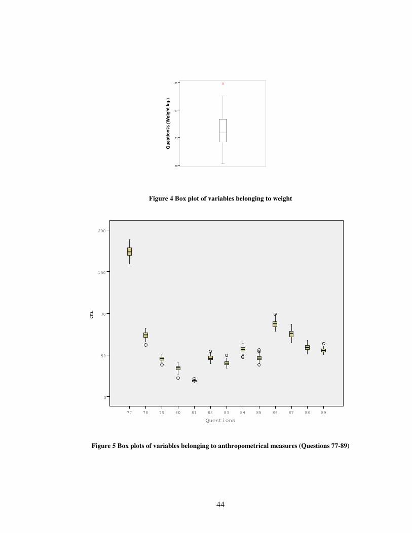
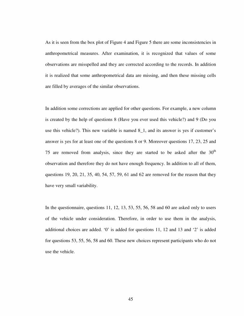
Firstly anomaly detection method is applied to data to check whether there are any

outliers or not. Anomaly modeling node in SPSS Clementine 10.1 does not detect any

outlier. After that inconsistencies and spelling errors among attributes are examined.

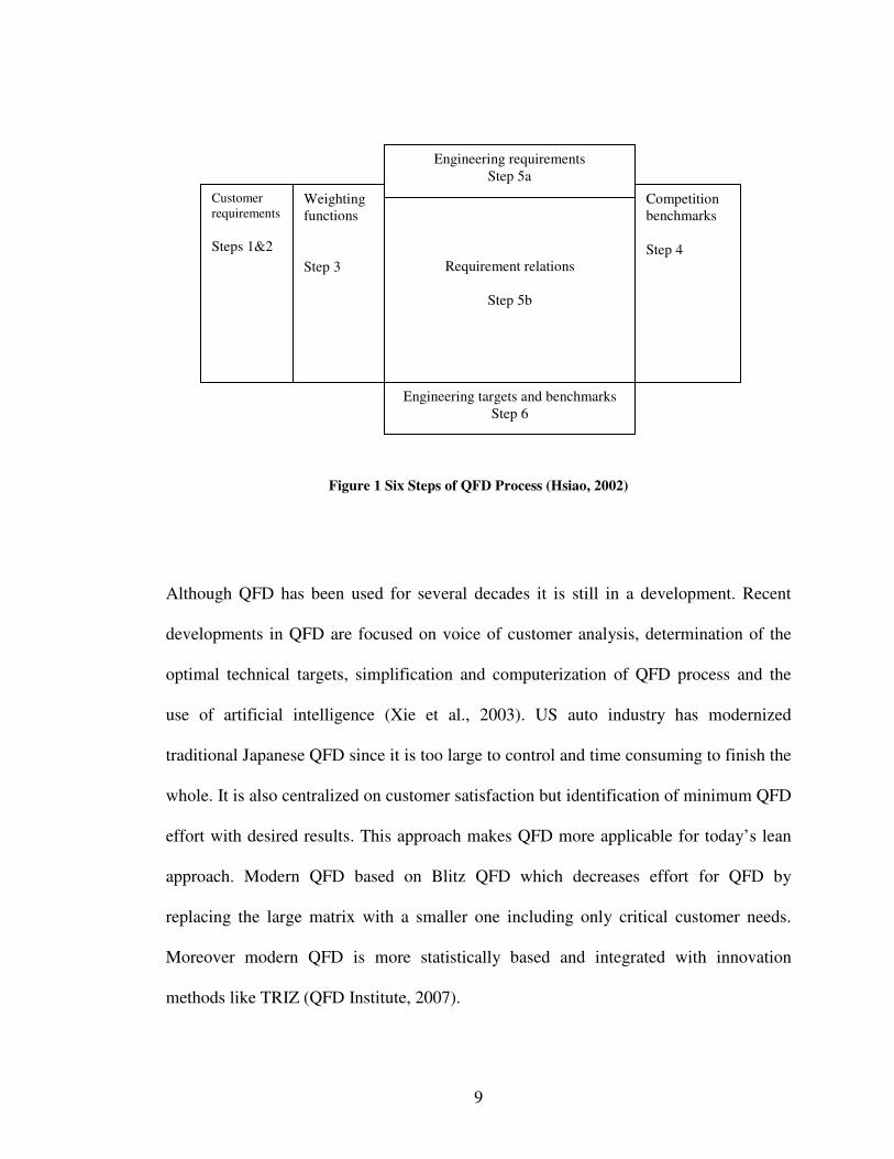
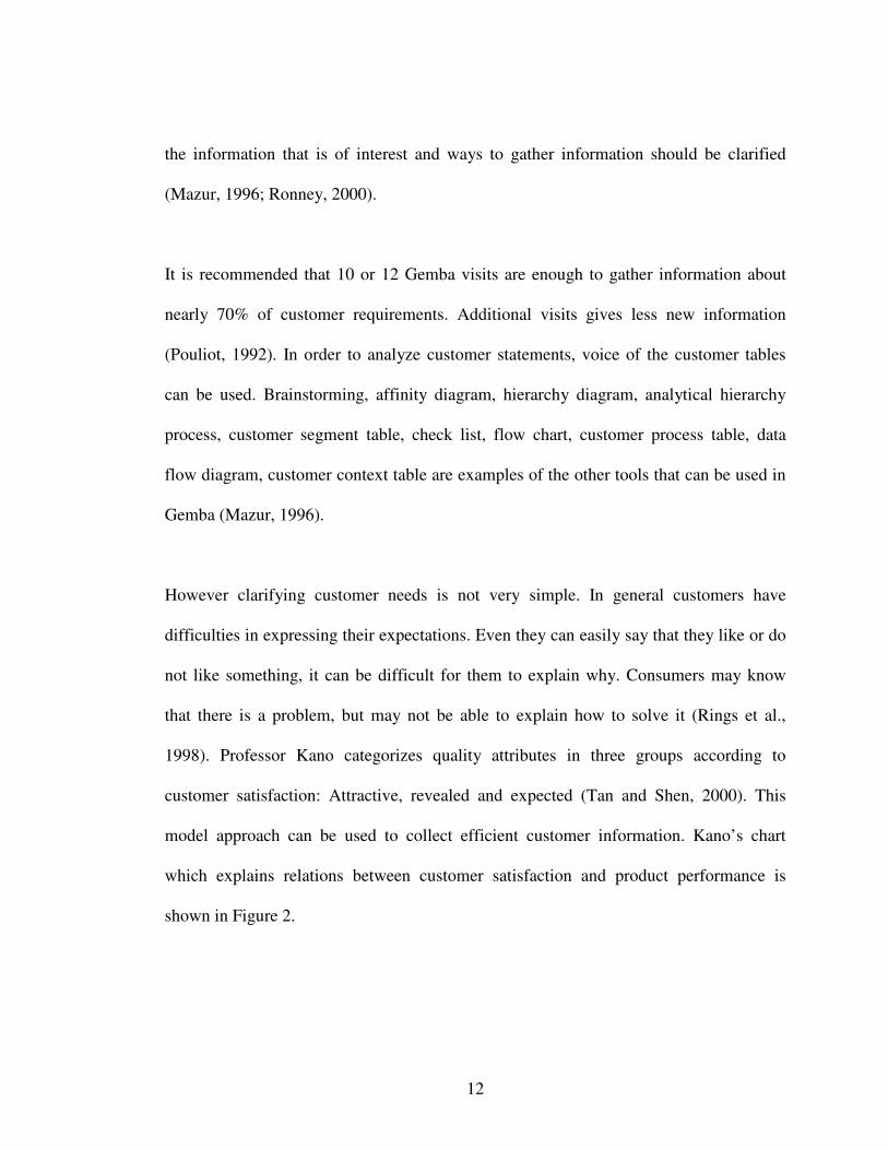
Box plots are plotted in order to examine interval type values (anthropometrical

measures).

44

50

75

100

125

Qu

es

tio

n76

(W

eig

ht

kg

.)

A

Figure 4 Box plot of variables belonging to weight

89888786858483828180797877

200

150

100

50

0

Questions

Figure 5 Box plots of variables belonging to anthropometrical measures (Questions 77-89)

cm.

45

As it is seen from the box plot of Figure 4 and Figure 5 there are some inconsistencies in

anthropometrical measures. After examination, it is recognized that values of some

observations are misspelled and they are corrected according to the records. In addition

it is realized that some anthropometrical data are missing, and then these missing cells

are filled by averages of the similar observations.

In addition some corrections are applied for other questions. For example, a new column

is created by the help of questions 8 (Have you ever used this vehicle?) and 9 (Do you

use this vehicle?). This new variable is named 8_1, and its answer is yes if customer’s

answer is yes for at least one of the questions 8 or 9. Moreover questions 17, 23, 25 and

75 are removed from analysis, since they are started to be asked after the 30th

observation and therefore they do not have enough frequency. In addition to all of them,

questions 19, 20, 21, 35, 40, 54, 57, 59, 61 and 62 are removed for the reason that they

have very small variability.

In the questionnaire, questions 11, 12, 13, 53, 55, 56, 58 and 60 are asked only to users

of the vehicle under consideration. Therefore, in order to use them in the analysis,

additional choices are added. ‘0’ is added for questions 11, 12 and 13 and ‘2’ is added

for questions 53, 55, 56, 58 and 60. These new choices represent participants who do not

use the vehicle.

46

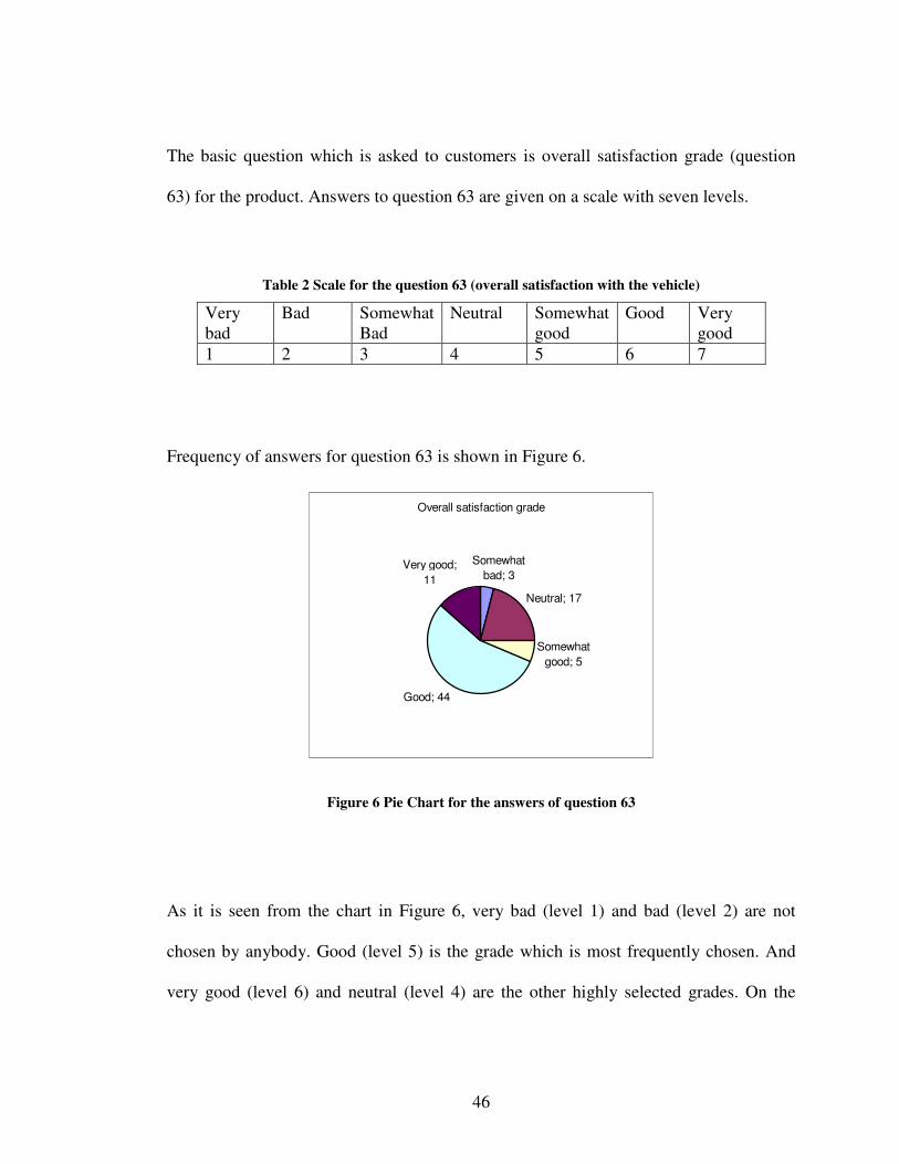
The basic question which is asked to customers is overall satisfaction grade (question

63) for the product. Answers to question 63 are given on a scale with seven levels.

Table 2 Scale for the question 63 (overall satisfaction with the vehicle)

Very bad

Bad Somewhat Bad

Neutral Somewhat good

Good Very good

1 2 3 4 5 6 7

Frequency of answers for question 63 is shown in Figure 6.

Overall satisfaction grade

Somewhat

bad; 3

Neutral; 17

Somewhat

good; 5

Good; 44

Very good;

11

Figure 6 Pie Chart for the answers of question 63

As it is seen from the chart in Figure 6, very bad (level 1) and bad (level 2) are not

chosen by anybody. Good (level 5) is the grade which is most frequently chosen. And

very good (level 6) and neutral (level 4) are the other highly selected grades. On the

47

other hand somewhat bad (level 3) and somewhat good (level 5) are selected just a few

times.

Since zero frequency or low frequencies, in outcome levels, cause problems in a logistic

regression model (see Section 2.2), scale of question 63 is converted. Firstly scale is

converted to three levels. However by using three levels, numerical problems could not

be eliminated from the model. Therefore the scale of this question is transformed to a

binary scale as shown in Table 3.

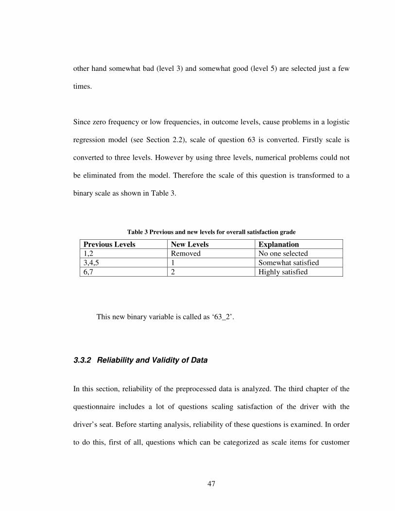
Table 3 Previous and new levels for overall satisfaction grade

Previous Levels New Levels Explanation 1,2 Removed No one selected 3,4,5 1 Somewhat satisfied 6,7 2 Highly satisfied

This new binary variable is called as ‘63_2’.

3.3.2 Reliability and Validity of Data

In this section, reliability of the preprocessed data is analyzed. The third chapter of the

questionnaire includes a lot of questions scaling satisfaction of the driver with the

driver’s seat. Before starting analysis, reliability of these questions is examined. In order

to do this, first of all, questions which can be categorized as scale items for customer

48

satisfaction are separated from the others. These questions are 15, 16, 22, 24, 28, 29, 30,

31-34, 36-39, 42-53, 55, 56, 58, 60, 63_2.

These questions are mixed with non-scale type of questions in the questionnaire and

hence, checking order of these questions is meaningless. Therefore it is decided to use

internal consistency method instead of split-half method. In order to examine internal

consistency reliability Kuder-Richardson formula 20 (KR-20) is calculated, since scores

are binary.

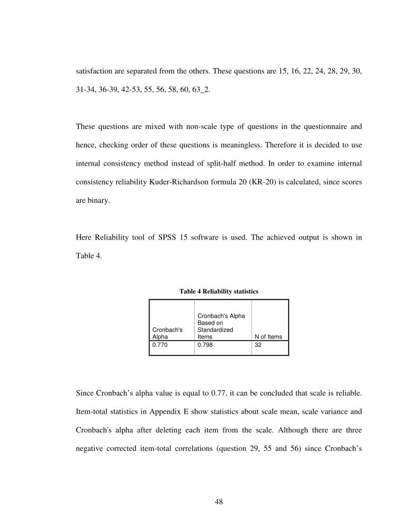
Here Reliability tool of SPSS 15 software is used. The achieved output is shown in

Table 4.

Table 4 Reliability statistics

Cronbach's Alpha

Cronbach's Alpha Based on Standardized Items N of Items

0.770 0.798 32

Since Cronbach’s alpha value is equal to 0.77, it can be concluded that scale is reliable.

Item-total statistics in Appendix E show statistics about scale mean, scale variance and

Cronbach's alpha after deleting each item from the scale. Although there are three

negative corrected item-total correlations (question 29, 55 and 56) since Cronbach’s

49

alpha does not increase sharply after deleting them, it is decided to keep them in the

analysis.

Since reliable scale does not guarantee that the latent variable is reasonable, validity of

scales should also be discussed. Validity is an issue which can be achieved by using

logic and experiences of experts. In this study, during questionnaire preparation phase, it

is discussed whether the used scales are representative for content domain or not. Here

QFD team members from production and marketing have given valuable information by

using their experiences and knowledge. Then empirical associations between scales and

some criteria are debated with them.

3.3.3 Simple Statistics

Before starting to apply an advanced statistical method to model overall satisfaction

grade, basic graphical analysis is performed. Some of these graphs are shown in

Appendix F. By using these graphs some insights are obtained about the data concerning

questions similar to the following:

• Which parts of the seat cause most dissatisfaction?

• Does the satisfaction from the arm rest change according to driver’s height and

weight?

• Does the height of driver affect satisfaction with the head restraint?

50

• Is there any relationship between lumbar support and weight of driver?

These examples can be extended. Although these analyses help the researcher to have an

opinion about how the data behave, they are not sufficient to develop a conclusion. The

first reason is that simple statistical analyses can continue to test other hypotheses, and

there are many hypotheses that can be formulated. It is not profitable to analyze all of

them, since it takes too much time to conclude. Secondly by using advanced data

analysis a mathematical model which can represent whole data can be developed. By

using this model, it is possible to estimate how much a given customer profile is to be

satisfied. Moreover generalizations about entire product users with a particular error can

be built. In addition optimization studies can be applied to mathematical models to find

out levels of factors that produce the most or the least desirable satisfaction grades.

3.3.4 Factor Analysis

Factor analysis is a method to find out the structure of interrelations between variables.

The starting point of factor analysis is correlation matrix (see Section 2.4). Therefore, in

order to eliminate multi collinearity that can occur in the model, first of all the

correlation matrix is built.

51

Since in the questionnaire there are some questions which are asked only to users of the

vehicle, two correlation matrices are constituted. First correlation matrix is built to

examine correlations between questions asked to every participant. Correlations, grater

than 0.5 are shown in Appendix G. Second correlation matrix is built to examine

correlations between questions asked only users of the vehicle and correlations between

these questions and the other ones asked to every participant. While analyzing

correlation matrices the correlations equal to or grater than 0.5 are considered as

significant.

According to the first correlation matrix the following result are observed (see Appendix

G):

• There are

o 0.846 correlation between questions 11 (How many km.s do you make

with this vehicle in a year?), and 8_1 (Have you ever used this vehicle?)

o 0.894 correlation between questions 12 (Why do you use this vehicle?)

and 8_1 (Have you ever used this vehicle?)

o 0.863 correlation between questions 13 (How frequently do you use this

vehicle?) and 8_1 (Have you ever used this vehicle?)

This result is not surprising since question 8_1 is asking if the vehicle is ever used

and the other questions (11, 12, and 13) apply for people who use it. Detailed

information about usage of vehicle can be acquired from questions 11, 12 and 13.

52

Hence, it is concluded not to use question 8_1 in the model when questions 11, 12

or 13 are used.

• There are

o 0.629 correlation between questions 33 (access to back angle adjustment)

and 32 (access to vertical adjustment)

o 0.537 correlation between questions 34 (access to lumbar support

adjustment) and 32 (access to vertical adjustment)

o 0.486 correlation between questions 34 (access to lumbar support

adjustment) and 33 (access to back angle adjustment)

This result is not surprising since accessibility to the adjustments asked in the above

questions involve mechanism located very near to each other at the left side of the seat.

Therefore it is decided to use only one of these questions in the analysis (see Section

3.3.6).

• There are

o 0.939 correlation between questions 45 (Do you like color of flash grey?)

and 49 (Do you like pattern of flash grey?)

o 0.925 correlation between questions 46 (Do you like color of flash red?)

and 50 (Do you like pattern of flash red?)

o 0.927 correlation between questions 47 (Do you like color of video

grey?) and 51 (Do you like pattern of video grey?)

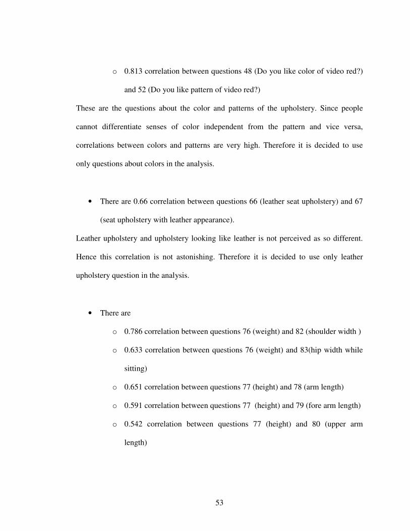
53

o 0.813 correlation between questions 48 (Do you like color of video red?)

and 52 (Do you like pattern of video red?)

These are the questions about the color and patterns of the upholstery. Since people

cannot differentiate senses of color independent from the pattern and vice versa,

correlations between colors and patterns are very high. Therefore it is decided to use

only questions about colors in the analysis.

• There are 0.66 correlation between questions 66 (leather seat upholstery) and 67

(seat upholstery with leather appearance).

Leather upholstery and upholstery looking like leather is not perceived as so different.

Hence this correlation is not astonishing. Therefore it is decided to use only leather

upholstery question in the analysis.

• There are

o 0.786 correlation between questions 76 (weight) and 82 (shoulder width )

o 0.633 correlation between questions 76 (weight) and 83(hip width while

sitting)

o 0.651 correlation between questions 77 (height) and 78 (arm length)

o 0.591 correlation between questions 77 (height) and 79 (fore arm length)

o 0.542 correlation between questions 77 (height) and 80 (upper arm

length)

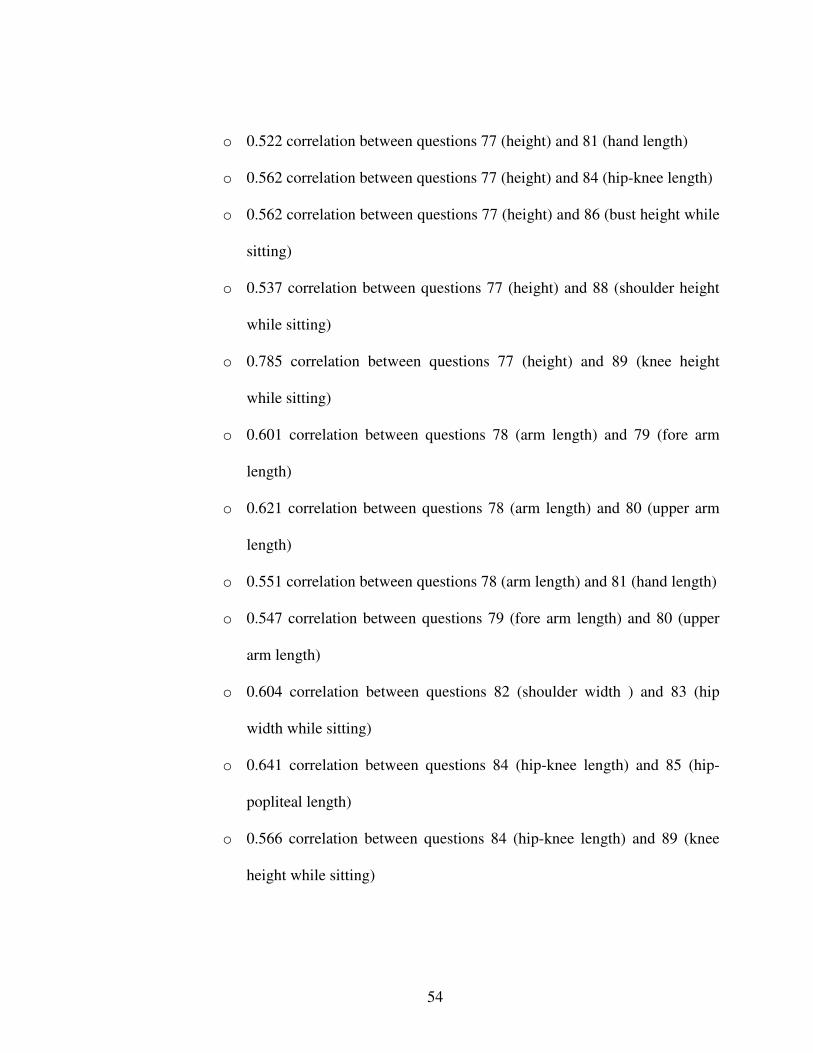
54

o 0.522 correlation between questions 77 (height) and 81 (hand length)

o 0.562 correlation between questions 77 (height) and 84 (hip-knee length)

o 0.562 correlation between questions 77 (height) and 86 (bust height while

sitting)

o 0.537 correlation between questions 77 (height) and 88 (shoulder height

while sitting)

o 0.785 correlation between questions 77 (height) and 89 (knee height

while sitting)

o 0.601 correlation between questions 78 (arm length) and 79 (fore arm

length)

o 0.621 correlation between questions 78 (arm length) and 80 (upper arm

length)

o 0.551 correlation between questions 78 (arm length) and 81 (hand length)

o 0.547 correlation between questions 79 (fore arm length) and 80 (upper

arm length)

o 0.604 correlation between questions 82 (shoulder width ) and 83 (hip

width while sitting)

o 0.641 correlation between questions 84 (hip-knee length) and 85 (hip-

popliteal length)

o 0.566 correlation between questions 84 (hip-knee length) and 89 (knee

height while sitting)

55

o 0.840 correlation between questions 86 (bust height while sitting) and 87

(eye height while sitting)

o 0.778 correlation between questions 86 (bust height while sitting) and 88

(shoulder height while sitting)

o 0.783 correlation between questions 87 (eye height while sitting) and 88

(shoulder height while sitting)

The correlations listed above show that anthropometrical measures form some groups.

Some of these groups are listed as follows:

• questions 76 (weight) , 82 (shoulder width ) and 83 (hip width while sitting)

• questions 77 (height), 78 (arm length) , 79 (fore arm length) , 80 (upper arm

length) and 81 (hand length)

• questions 86 (bust height while sitting) , 87 (eye height while sitting) and 88

(shoulder height while sitting)

• questions 84 (hip-knee length) and 85 (hip-popliteal length)

• question 89 (knee height while sitting) and 77 (height)

The second correlation matrix which is built to examine correlation between questions

asked to users of the vehicles and correlation between these questions and the other ones

asked to every participant does not add any more information other than the results

acquired by the first correlation matrix. Therefore only the first correlation matrix is

considered in the following analysis.

56

In order to understand groups or clusters formed by questions and factors behind of

these groups, factor analysis is applied. While building the model, one representative

from each group is selected to be used. In addition, principle components are built to

form new uncorrelated variables which are linear composites of original variables.

Factor analysis is applied to anthropometrical measures (see Appendix H) and other

discrete questions which can be treated as metric variable (see Appendix H) separately.

After applying factor analysis for anthropometrical measures 4 factors are derived.

� Factor 1 is formed by questions 77 (height), 78 (arm length), 79 (fore arm

length), 80 (upper arm length), 81 (hand length) and 89 (knee height while

sitting).

Common property: Measures about driver’s ability to reach somewhere in the

vehicle.

� Factor 2 is formed by questions 86 (bust height while sitting), 87 (eye height

while sitting) and 88 (shoulder height while sitting).

Common property: Measures about driver’s height while sitting on the seat.

57

� Factor 3 is formed by question 76 (weight), 82 (shoulder width) and 83 (hip

width while sitting).

Common property: Measures about driver’s body width.

� Factor 4 is formed by question 84 (hip-knee length) and 85 (hip-popliteal length).

Common property: Measures about driver’s upper leg length while sitting on the

seat.

These factors derived are used in the course of determining the independent variables to

be used in the model (see Section 3.3.6).

Concerning factor analysis of questions about comfort (Appendix H), we observe that

some of the communalities are very low (less than 0.5) and about 12 factors can be

chosen for 36 questions. In addition most of the factors have 2 or 1 variables. In order to

say that a variable belongs to a factor, its loading in that factor should be significantly

bigger than the others. As it is seen in the Appendix H, some variables do not have a

loading which is significantly bigger than the others. Because of these reasons, factors

generated by the factor analysis for questions about comfort are not used in the

following analysis. Instead of it, information from correlation matrix is taken into

account.

58

Principle Components Analysis

Principle component analysis is used in order to form independent variables from

correlated continuous variables (anthropometrical measures). Before applying it, data is

standardized by using the following coding formula (Mendenhall and Sincich, 1996):

ii

X

x xStdx

s

−= [3.6]

In the equation [3.6]

xi : ith uncoded quantitative variable

Stdxi : ith coded quantitative variable

ix

xn

=∑ [3.7]

where n is the sample size

2( )

1i

x

x xs

n

−=

−

∑ [3.8]

The derived principle components are shown in Appendix I. Since eigenvalues are less

than one after the 4th principle component, four principle components are used in the

analysis. The obtained principle components (PCs) are given in Equations [3.9], [3.10],

[3.11], and [3.12].

59

PC1 = 0.224 Std76 + 0.368 Std77 + 0.301 Std78 + 0.277 Std79 + 0.276 Std80 + 0.252

Std81 + 0.238 Std82 + 0.166 Std83 + 0.280 Std84 + 0.177 Std85 + 0.287 Std86 + 0.227

Std87 + 0.278 Std88 + 0.319 Std8 [3.9]

PC2 = -0.465 Std76 + 0.037 Std77 + 0.094 Std78 + 0.093 Std79 + 0.037 Std80 - 0.042

Std81 - 0.386 Std82 - 0.447 Std83 - 0.025 Std84 - 0.006 Std85 + 0.330 Std86 + 0.428

Std87 + 0.340 Std88 - 0.073 Std89 [3.10]

PC3 = -0.271 Std76+ 0.081 Std77 + 0.304 Std78 + 0.267 Std79 + 0.180 Std80 + 0.077

Std81 - 0.323 Std82 - 0.266 Std83 + 0.282 Std84 + 0.358 Std85 - 0.335 Std86 - 0.367

Std87 - 0.279 Std88 + 0.101 Std89 [3.11]

PC4 = -0.069 Std76 + 0.006 Std77 + 0.292 Std78 + 0.308 Std79 + 0.232 Std80 + 0.437

Std81 + 0.012 Std82 - 0.071 Std83 - 0.421 Std84 - 0.590 Std85 - 0.033 Std86 - 0.056

Std87 - 0.116 Std88 - 0.151 Std89 [3.12]

(Note that Stdx is the standardized value of the answer given to question x.)

Generated principle components are used as variables instead of anthropometrical

measures in the logistic regression modeling. The drawback of principle components is

the difficulty of their interpretation. Still, the principle components are tried to be

60

interpreted by using scatter plots of them versus anthropometrical measures (see

Appendix J). Scatter plots are used to understand the relations between principle

components and anthropometrical measures.

Plots in Appendix J show that principle component 1 (PC1) is positively related with

each anthropometrical measure.

Plots in Appendix J show that principle component 2 (PC2) is negatively related with

questions 76 (weight), 82 (shoulder width), and 83 (hip width while sitting) and it is

positively related with questions 86 (bust height while sitting), 87 (eye height while

sitting), and 88 (shoulder height while sitting). Therefore, it can be concluded that

principle component 2 is decreasing while measures about driver’s body wideness are

increasing, and it is increasing while measures about driver’s height when sitting on the

seat are increasing.

Plots in Appendix J show that principle component 3 (PC3) is negatively related with

questions 76 (weight), 82 (shoulder width), 83 (hip width while sitting), 86 (bust height

while sitting), 87 (eye height while sitting) and 88 (shoulder height while sitting) and it

is positively related with questions 78 (arm length), 79 (fore arm length) and 80 (upper

arm length). This means that principle component 3 is decreasing while measures about

driver’s body wideness and measures about driver’s height when sitting on the seat are

increasing, and it is increasing while measures about arm length of driver are increasing.

61

Plots in Appendix J show that principle component 4 (PC4) is negatively related with

questions 84 (hip-knee length) and 85 (hip-popliteal length) and it is positively related

with questions 78 (arm length), 79 (fore arm length), 80 (upper arm length), and 81

(hand length). Therefore, it can be concluded that principle component 4 is decreasing

while measures about upper leg length when sitting on the seat are increasing, and is

increasing while measures about arm length of driver are increasing.

3.3.5 Models for Questions about Comfort

Before building a logistic regression model for overall satisfaction grade an analysis

about which variables should be used as predictors in the model is made. The main

argument is that there can be cause-effect relations between comfort related questions

and the others. Especially it is debated that anthropometrical measures and some

characteristic of a customer and his/her vehicle usage preferences can explain his/her

comfort and access to parts of the seat and the vehicle.

In spite of the fact that the correlation matrix does not show any strong correlations

between such questions, in order to be sure logistic regression models of these comfort

related questions are built.

62

After analyzing such logistic regression models, it is figured out that none of the comfort

questions could be strongly explained by any anthropometrical measures or any other

questions. Therefore it is concluded to use every kind of questions in the questionnaire

while forming logistic regression model.

3.3.6 Logistic Regression Analysis for Overall Satisfaction Grade

Covariates in the Model Since models examined in Section 3.3.5 are not significant, it is decided to use all

relevant questions and anthropometrical measures in the logistic regression model.

While using them, results obtained by correlation matrices, factor analysis and principle

component analysis are taken into account. According to the result of correlation matrix,

obtained in the Section 3.3.4, some variables about comfort are removed from the

analysis.

Correlation matrix, in Appendix G, show that there are significant correlations between

question 8_1 (Have you ever used this vehicle?) and questions 11 (How many km.s do

you make with this vehicle in a year?), 12 (Why do you use this vehicle?) and 13 (How

frequently do you use this vehicle?). Since questions 11, 12 and 13 are investigated in

the model, question 8_1 is not used.

63

In addition questions 32 (access to vertical adjustment), 33 (access to back angle

adjustment) and 34 (access to lumbar support adjustment) are correlated. While selecting

representative among them, correlations between these question and question 63_2

(overall satisfaction grade modified to two levels) is considered. Correlation between

questions 32 and 63_2 is 0.313, correlation between questions 33 and 63_2 is 0.396 and

correlation between questions 34 and 63_2 is 0.319. Since question 33 has the strongest

correlation with question 63_2, it is selected as representative. In addition, three of these

adjustments are located on the left side of the seat. The order of these adjustments from

the front is like: vertical, seat back and lumbar support. Due to seat back adjustment

being in the middle, it is meaningful to select it as representative.

For each upholstery styles, question about color and question about pattern are highly

correlated (see Section 3.3.4). Between upholstery color and upholstery pattern

questions, color questions are selected as representative for each style of upholstery.

Thence the representatives in the model are questions 45 (color of flash grey), 46 (color

of flash red), 47 (color of video grey) and 48 (color of video red).

Finally, since there is a big correlation between questions 66 (leather seat upholstery)

and 67 (seat upholstery with leather appearance), question 66 is selected as

representative.

64

For anthropometrical measures, results attained by factor analysis and principle

component analysis (see Section 3.3.4) are used.

Logistic Regression Models for Question 63_2 (Overall Satisfaction Grade Modified in Two Levels)

In order not to get any multicollinearity problem in the model (see Section 2.2), results

extracted by correlation matrices are used for questions about vehicle usage and driver’s

comfort (questions 1-75). In addition, results obtained by factor analysis and principle

component analysis are used for anthropometrical data (questions 76-89). Eventually, 55

input variables are used to build the model.

Since two way interactions can be influential, they are also handled in the model. If

hierarchical structure is used, each main effect which is forming interactions should exist

in the model. Since level frequencies of covariates and factors are not balanced in the

data, increasing the number of covariates in the model can result to have complete or

quasi complete separation problem (see section 2.2). When this problem occurs because

of some main effects, interactions should be removed from the model with the

problematic main effects. Therefore hierarchical structure is not used while examining

interactions. Moreover some covariates that cause complete and quasi-complete

separation are removed (Question 1 (Gender), question 5 (Do you live with your

family?), question 56 (Do you feel any pain or discomfort in your neck while you are

driving?), question 58 (Do you feel any pain or discomfort in your popliteal while you

65

are driving?), question 60 (Do you feel any pain or discomfort in your lower leg while

you are driving?)).

In order not to have problems about multicollinearity, two different methods which

make use of factor analysis and principle components, respectively, are applied. Thus

two alternative models are obtained.

Güntürkün (2007) applies decision tree analysis for these data in another study. The

decision tree derived in that study is shown in Appendix K. In the current study, it is also

made use of this thesis while discussing the predictors of the models. According to these

discussions:

• While building model 1, question 27 (Do you expect from the head restraint to

rest your head?) is removed from the model since it is not strongly significant.

However, since the decision tree has question 27, it is decided to compare the

model containing question 27 with the model which is not containing it. Their

statistics are shown in the following table:

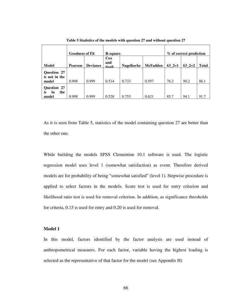
66

Table 5 Statistics of the models with question 27 and without question 27

Goodness of Fit R-square % of correct prediction

Model Pearson Deviance

Cox and Snell Nagelkerke McFadden 63_2=1 63_2=2 Total

Question 27 is not in the model 0.998 0.999 0.514 0.733 0.597 76.2 90.2 86.1

Question 27 is in the model 0.998 0.999 0.528 0.753 0.621 85.7 94.1 91.7

As it is seen from Table 5, statistics of the model containing question 27 are better than

the other one.

While building the models SPSS Clementine 10.1 software is used. The logistic

regression model uses level 1 (somewhat satisfaction) as event. Therefore derived

models are for probability of being “somewhat satisfied” (level 1). Stepwise procedure is

applied to select factors in the models. Score test is used for entry criterion and

likelihood ratio test is used for removal criterion. In addition, as significance thresholds

for criteria, 0.15 is used for entry and 0.20 is used for removal.

Model 1 In this model, factors identified by the factor analysis are used instead of

anthropometrical measures. For each factor, variable having the highest loading is

selected as the representative of that factor for the model (see Appendix H)

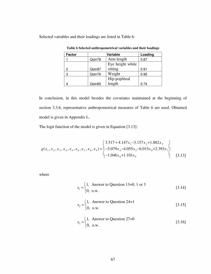
67

Selected variables and their loadings are listed in Table 6:

Table 6 Selected anthropometrical variables and their loadings

Factor Variable Loading

1 Qstn78 Arm length 0.87

2 Qstn87

Eye height while sitting 0.91

3 Qstn76 Weight 0.95

4 Qstn85

Hip-popliteal length 0.74

In conclusion, in this model besides the covariates maintained at the beginning of

section 3.3.6, representative anthropometrical measures of Table 6 are used. Obtained

model is given in Appendix L.

The logit function of the model is given in Equation [3.13]:

[3.13]

where

1

1, Answer to Question 13=0, 1 or 3

0, o.w.x

=

[3.14]

2

1, Answer to Question 24=1

0, o.w.x

=

[3.15]

3

1, Answer to Question 27=0

0, o.w.x

=

[3.16]

1 2 3

1 2 3 4 5 6 7 8 9 4 5 6 7

8 9

3.517 4.147 3.157 1.882

( , , , , , , , , ) 5.079 4.055 6.015 2.393

1.046 1.101

x x x

g x x x x x x x x x x x x x

x x

+ − +

= − − − + − +

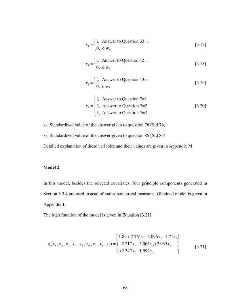
68

4

1, Answer to Question 33=1

0, o.w.x

=

[3.17]

5

1, Answer to Question 42=1

0, o.w.x

=

[3.18]

6

1, Answer to Question 43=1

0, o.w.x

=

[3.19]

7

1, Answer to Question 7=1

2, Answer to Question 7=2

3, Answer to Question 7=3

x

=

[3.20]

x8: Standardized value of the answer given to question 76 (Std 76)

x9: Standardized value of the answer given to question 85 (Std 85)

Detailed explanation of these variables and their values are given in Appendix M.

Model 2

In this model, besides the selected covariates, four principle components generated in

Section 3.3.4 are used instead of anthropometrical measures. Obtained model is given in

Appendix L.

The logit function of the model is given in Equation [3.21]:

[3.21]

1 2 3

1 2 3 4 5 6 7 8 9 4 5 6

7 8

1.89 2.761 3.096 4.71

( , , , , , , , , ) 2.217 5.065 2.935

2.347 1.992

x x x

g x x x x x x x x x x x x

x x

+ − −

= − − + + +

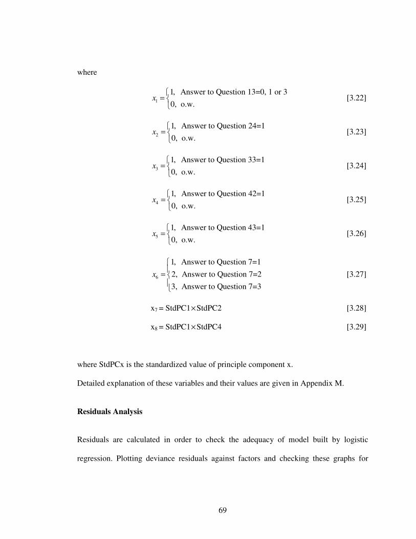
69

where

1

1, Answer to Question 13=0, 1 or 3

0, o.w.x

=

[3.22]

2

1, Answer to Question 24=1

0, o.w.x

=

[3.23]

3

1, Answer to Question 33=1

0, o.w.x

=

[3.24]

4

1, Answer to Question 42=1

0, o.w.x

=

[3.25]

5

1, Answer to Question 43=1

0, o.w.x

=

[3.26]

6

1, Answer to Question 7=1

2, Answer to Question 7=2

3, Answer to Question 7=3

x

=

[3.27]

x7 = StdPC1×StdPC2 [3.28]

x8 = StdPC1×StdPC4 [3.29]

where StdPCx is the standardized value of principle component x.

Detailed explanation of these variables and their values are given in Appendix M.

Residuals Analysis Residuals are calculated in order to check the adequacy of model built by logistic

regression. Plotting deviance residuals against factors and checking these graphs for

70

patterns or outliers helps to check model fit. Analysis of residuals is performed by

examining two types of graphs (see Appendix N). Graph 1 is used to check whether

deviance residuals show a pattern according to the order of data collection or whether

there are any outliers in data. This plot is a plot of deviance residuals versus their index

number (collection order). If this graph does not show any pattern, it can be concluded

that residuals are randomly distributed according to the index. Graph 2 is used to check

whether deviance residuals show a pattern according to levels of factors. If this graph

does not show any pattern, it can be concluded that residual values do not change

according to the levels of factors. However this method is an exploratory type to check

model adequacy. Durbin-Watson Statistics can be used to confirm the adequacy of the

model (Verbeek, 2004) If there is autocorrelation in the residuals from the model, marginal

modeling analysis or transitional models can be used (Wu and Zhang, 2006)

As it is seen in Appendix N; none of the graphs show any pattern or outlier. Hence, we

conclude that the generated models are adequate.

Comparison of the Two Models In order to investigate whether or not one of the models is better than the other,

comparison of these two models is made. During this comparison; statistics, estimated

probabilities, and confidence intervals of estimated probabilities are used.

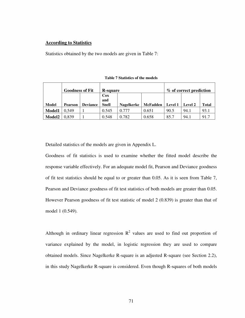
71

According to Statistics Statistics obtained by the two models are given in Table 7:

Table 7 Statistics of the models

Goodness of Fit R-square % of correct prediction

Model Pearson Deviance

Cox and Snell Nagelkerke McFadden Level 1 Level 2 Total

Model1 0,549 1 0.545 0.777 0.651 90.5 94.1 93.1

Model2 0,839 1 0.548 0.782 0.658 85.7 94.1 91.7

Detailed statistics of the models are given in Appendix L.

Goodness of fit statistics is used to examine whether the fitted model describe the

response variable effectively. For an adequate model fit, Pearson and Deviance goodness

of fit test statistics should be equal to or greater than 0.05. As it is seen from Table 7,

Pearson and Deviance goodness of fit test statistics of both models are greater than 0.05.

However Pearson goodness of fit test statistic of model 2 (0.839) is greater than that of

model 1 (0.549).

Although in ordinary linear regression R2 values are used to find out proportion of

variance explained by the model, in logistic regression they are used to compare

obtained models. Since Nagelkerke R-square is an adjusted R-square (see Section 2.2),

in this study Nagelkerke R-square is considered. Even though R-squares of both models

72

are very near to each other, Nagelkerke R-square of model 2 (0.782) is greater than that

of model 1 (0.777).

Percent (%) of correct predictions show the percentage of the data predicted correctly by

the model. Both of the models predict level 2 (highly satisfied) better than level 1

(somewhat satisfied). This result is not surprising since, in the data, level 1 is observed

less than level 2 (25 participants selected level 1, 55 participants selected level 2). For

level 2 both of the models have the same correct prediction rate (94.1 %). However, in

model 1, level 1 is predicted better (90.5% > 85.7%). In total, model 1 predicts better

than model 2 (93.1%>91.7%).

According to Estimated Probability

In this study estimated probabilities by the models are the probabilities that a customer is

somewhat satisfied with the driver’s seat. This is level 1 of the question 63_2 (overall

satisfaction grade modified in two levels). Here estimated probabilities for level 1

(somewhat satisfied) by the two models are compared. Figure 7 shows a histogram of

the differences between estimated probabilities of observing level 1 of the two models.

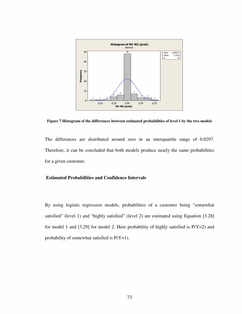
73

0,320,160,00-0,16-0,32

50

40

30

20

10

0

M1-M2 (prob)

Frequency

Mean -0,003217

StDev 0,1074

N 75

133

7

48

64

111

Histogram of M1-M2 (prob)Normal

Figure 7 Histogram of the differences between estimated probabilities of level 1 by the two models

The differences are distributed around zero in an interquartile range of 0.0297.

Therefore, it can be concluded that both models produce nearly the same probabilities

for a given customer.

Estimated Probabilities and Confidence Intervals

By using logistic regression models, probabilities of a customer being “somewhat

satisfied” (level 1) and “highly satisfied” (level 2) are estimated using Equation [3.28]

for model 1 and [3.29] for model 2. Here probability of highly satisfied is P(Y=2) and

probability of somewhat satisfied is P(Y=1).

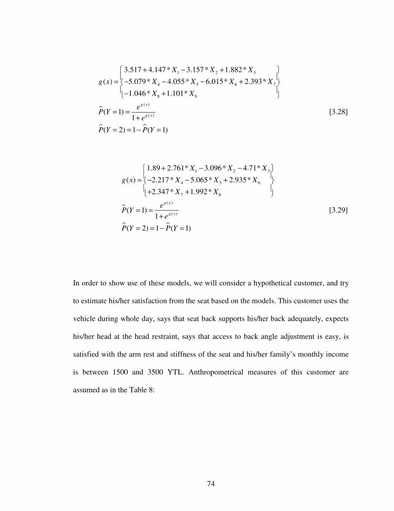
74

�

� �

1 2 3

4 5 6 7

8 9

( )

( )

3.517 4.147* 3.157* 1.882*

( ) 5.079* 4.055* 6.015* 2.393*

1.046* 1.101*

( 1)1

( 2) 1 ( 1)

g x

g x

X X X

g x X X X X

X X

eP Y

e

P Y P Y

+ − +

= − − − + − +

= =+

= = − =

[3.28]

�

� �

1 2 3

4 5 6

7 8

( )

( )

1.89 2.761* 3.096* 4.71*

( ) 2.217* 5.065* 2.935*

2.347* 1.992*

( 1)1

( 2) 1 ( 1)

g x

g x

X X X

g x X X X

X X

eP Y

e

P Y P Y

+ − −

= − − + + +

= =+

= = − =

[3.29]

In order to show use of these models, we will consider a hypothetical customer, and try

to estimate his/her satisfaction from the seat based on the models. This customer uses the

vehicle during whole day, says that seat back supports his/her back adequately, expects

his/her head at the head restraint, says that access to back angle adjustment is easy, is

satisfied with the arm rest and stiffness of the seat and his/her family’s monthly income

is between 1500 and 3500 YTL. Anthropometrical measures of this customer are

assumed as in the Table 8:

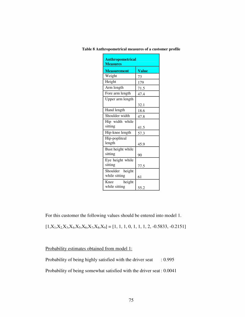
75

Table 8 Anthropometrical measures of a customer profile

Anthropometrical Measures

Measurement Value Weight 73 Height 179 Arm length 71.5 Fore arm length 47.4 Upper arm length

32.1 Hand length 18.6 Shoulder width 47.8 Hip width while sitting 41.5 Hip-knee length 57.3 Hip-popliteal length 45.9 Bust height while sitting 90 Eye height while sitting 77.5 Shoulder height while sitting 61 Knee height while sitting 55.2

For this customer the following values should be entered into model 1.

[1,X1,X2,X3,X4,X5,X6,X7,X8,X9] = [1, 1, 1, 0, 1, 1, 1, 2, -0.5833, -0.2151]

Probability estimates obtained from model 1:

Probability of being highly satisfied with the driver seat : 0.995

Probability of being somewhat satisfied with the driver seat : 0.0041

76

90% Confidence Intervals (CI) for the probabilities:

CI for being highly satisfied : [0.875 , 1.000]

CI for being somewhat satisfied : [0.000, 0.125]

Calculations for these CIs are shown in Appendix O and P.

For this customer the following values should be entered into model 2.

[1,X1,X2,X3,X4,X5,X6,X7,X8] = [1, 1, 1, 1, 1, 1, 2, 0.064,-0.05236]

Probability estimates obtained from model 2:

Probability of being highly satisfied with the driver seat : 0.989

Probability of being somewhat satisfied with the driver seat : 0.011

90% Confidence Intervals (CI) for the probabilities:

CI for being highly satisfied : [0.831 , 0.999]

CI for being somewhat satisfied : [0,001 , 0,169]

Calculations for CI are shown in Appendix O and P.

As it is mentioned in Section 2.2; in logistic regression, relationship between predicted

probabilities (Y) and independent variables (X) is in S shape. Therefore variation in

predicted probabilities is small while probabilities approach near 0 or 1, and the

77

variation increases while probabilities approach near 0.5. As it is seen in Appendix O,

confidence interval calculations use variance of probabilities. Therefore, the width of

confidence intervals, in logistic regression, narrows naturally while probabilities are near

0 or 1, and widens while probabilities move near 0.5.

However confidence intervals of the models in this study extend very fast. The first

reason is that there is a significant difference between frequencies of two levels of

dependent variable (overall satisfaction grade). 25 persons selected “somewhat satisfied”

and 55 persons selected “highly satisfied”. In addition, in the confidence interval

calculation, variance and covariance matrix of predicted coefficients is used. If variance

or covariance of estimated coefficients increases, this will cause an increase in the width

of confidence intervals. Since level frequencies of independent variables are not in a

good balance, variance or covariance of estimated coefficients are not very small. This

can cause the confidence interval width to increase.

3.4 Optimization and Prediction

The prediction models can provide us useful information whether or not a customer will

be satisfied from the seat. Optimization is applied to the logistic regression models to

find what kind of customers like (or dislike) the driver seat the most. Maximization or

78

minimization of overall satisfaction grade can also be helpful in finding design

improvement needs.

Microsoft Excel Solver is used to optimize the models. Excel uses Generalized Reduced

Gradient (GRG2) algorithm to optimize nonlinear problems. There is a possibility that

the algorithm can stop on a local optimum point since, the problem of this study is

nonlinear. Therefore obtained models are optimized and minimized 25 times. After that

it is seen that most of the optimizations stop when the P(Y=2)=1 and P(Y=1)=1. These

are the maximum values that a probability can be. It is observed that these optimizations

give the same values for categorical variables in the model. However they stop on

different values for continuous variables. While deciding on the optimum points of

continuous variables (anthropometrical measures) mean of the results obtained from

optimizations are used.

Optimization of Model 1

Optimization model of ‘Model 1’ is given in Appendix Q. According to this

optimization model, driver characteristics that maximize or minimize overall satisfaction

grade can be obtained as shown in Table 9.

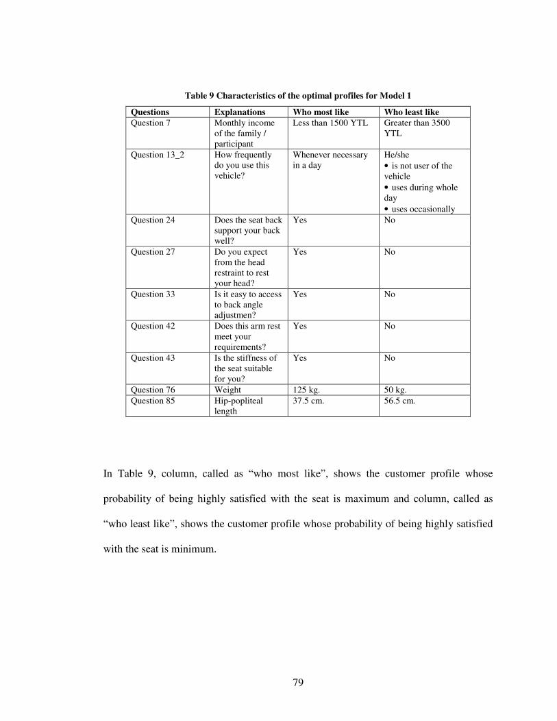
79

Table 9 Characteristics of the optimal profiles for Model 1

Questions Explanations Who most like Who least like Question 7 Monthly income

of the family / participant

Less than 1500 YTL Greater than 3500 YTL

Question 13_2 How frequently do you use this vehicle?

Whenever necessary in a day

He/she • is not user of the vehicle • uses during whole day • uses occasionally

Question 24 Does the seat back support your back well?

Yes No

Question 27 Do you expect from the head restraint to rest your head?

Yes No

Question 33 Is it easy to access to back angle adjustmen?

Yes No

Question 42 Does this arm rest meet your requirements?

Yes No

Question 43 Is the stiffness of the seat suitable for you?

Yes No

Question 76 Weight 125 kg. 50 kg. Question 85 Hip-popliteal

length 37.5 cm. 56.5 cm.

In Table 9, column, called as “who most like”, shows the customer profile whose

probability of being highly satisfied with the seat is maximum and column, called as

“who least like”, shows the customer profile whose probability of being highly satisfied

with the seat is minimum.

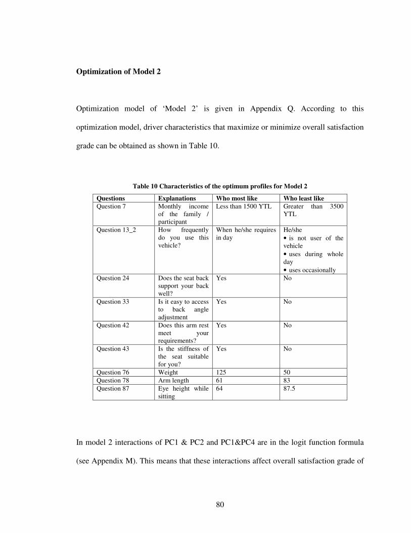
80

Optimization of Model 2

Optimization model of ‘Model 2’ is given in Appendix Q. According to this

optimization model, driver characteristics that maximize or minimize overall satisfaction

grade can be obtained as shown in Table 10.

Table 10 Characteristics of the optimum profiles for Model 2

Questions Explanations Who most like Who least like Question 7 Monthly income

of the family / participant

Less than 1500 YTL Greater than 3500 YTL

Question 13_2 How frequently do you use this vehicle?

When he/she requires in day

He/she • is not user of the vehicle • uses during whole day • uses occasionally

Question 24 Does the seat back support your back well?

Yes No

Question 33 Is it easy to access to back angle adjustment

Yes No

Question 42 Does this arm rest meet your requirements?

Yes No

Question 43 Is the stiffness of the seat suitable for you?

Yes No

Question 76 Weight 125 50 Question 78 Arm length 61 83 Question 87 Eye height while

sitting 64 87.5

In model 2 interactions of PC1 & PC2 and PC1&PC4 are in the logit function formula

(see Appendix M). This means that these interactions affect overall satisfaction grade of

81

customers. As it is mentioned in chapter 3.3.4, principle components are components

representing anthropometrical measures. Among these measures some of them are

expected to be more effective on the satisfaction grade. Some analyses are applied in

order to understand which measures affect satisfaction grade mostly and in which way.

Since there are infinitely many optimum points for model 2, different optimum levels for

anthropometrical measures are obtained by maximizing and minimizing model 2 for 18

times. This is done in order to obtain different optimal levels of anthropometrical

measures for high satisfaction (Y=2) by maximizing and somewhat satisfaction (Y=1)

by minimizing. Then these optimal values are plotted versus to the satisfaction grades 1

(somewhat) and 2 (highly) (see Appendix R). The aim to examine these individual plots

is to detect anthropometrical measures which have significantly different values for

somewhat and high satisfaction grades. As it is seen from graphs in Appendix R, values

of questions 76 (weight), 78 (arm length), and 87 (eye height while sitting) have

differences according to levels of satisfaction grade. Therefore these measures are

defined as the critical anthropometrical measures which affect satisfaction grade.

Results Obtained by Optimization Profiles of customers, satisfied with the seat the most or the least, obtained by

optimization of the models, help understand which features of the seat design should be

improved. For example the results show that probability of a person being satisfied with

the driver seat increases as his/her weight increases. This means that the seat should be

82

modified for satisfaction of light weight people as well. Similarly, people, who like

stiffness of the seat, like the driver seat more. Hence, stiffness should be studied by the

designer.

These types of conclusions have been extensively derived and presented to the company.

Due to confidentiality reasons, we are not allowed to present all of them in this report.

83

CHAPTER 4

DISCUSSION

In this study, a comprehensive analysis of customer requirements and satisfaction with a

certain driver’s seat is performed. The aim is discover opportunities to improve driver

seat design in the light of the analysis results. Data are collected observing and

questioning the customers while using the seat (Gemba studies). Before going to Gemba,

customer segments and profiles are determined. During Gemba visits appropriate

customers from the segments are selected to be observed. Observations are supported by

a questionnaire. This questionnaire includes free observations with open ended questions

as well as closed ended questions about comfort of the driver seat, and anthropometrical

measures.

Data analysis is started with simple statistics. This allows us to see general behavior of

the data and relationships in it. Then logistic regression is selected to be used since it is a

modeling technique for categorical responses. Before applying logistic regression,

relationships among the data are examined. Correlation matrix is used to detect highly

correlated variables in the data. Log Odds is another suggested method to analyze

84

correlations of binary variables. This approach can give more convenient results.

Therefore it can be suggested for the further studies.

Factor analysis and principle component analysis techniques are applied to

anthropometrical measures in order to obtain independent variables from them. While

factor analysis groups the data according to the correlations between them, principle

component analysis built independent variables which are linear functions of the raw

variables.

By using results of these two techniques two different logistic regression models are

developed. The first model is built by using one representative from each factor instead

of all anthropometrical measures. However in the second model, principle components

of the anthropometrical measures are used.

Both of the models have monthly income (question 7) as a demographic variable, and

among the questions about vehicle usage both of them include the frequency of the

vehicle usage (question 13). In addition both models include nearly the same questions

about comfort, appearance and usage of the driver seat. These are back support by the

seat back (questions 24), access to the back angle adjustment (question 33), satisfaction

with the arm rest (question 42) and satisfaction with the seat stiffness (question 43).

Besides them, model 1 includes question 27 which is expectation from head restraint to

rest driver’s head. Additionally model 1, which is built using representatives from factor

85

analysis, includes weight (question 76) and hip-popliteal length (question 85). However

model 2, which is formed by using principle components, includes interaction of PC1 &

PC2 and PC1&PC4. Since model 1 includes directly the anthropometrical measures it is

clearer to explain which measures affect the satisfaction grade and in which way.

However model 2 is more complex to understand which part of the body is influential on

the satisfaction. In order to make it clear, some more analyses are performed. In these

analyses firstly model 2 is maximized and minimized 18 times. Then individual value

plots of each anthropometrical measurement versus satisfaction grades 1 (somewhat

satisfied) and 2 (highly satisfied) are plotted. After that it is developed that weight

(questions 76), arm length (question 78), and eye height while sitting (question 87) are

effective on the satisfaction grade.

When these two models are compared statistically, goodness of fit test results, R-squares

and percent (%) of correction rates are examined, and significant differences are

observed between them. Although model 2 is better according to Pearson goodness of fit

statistic and R-squares, model 1 is better according to % correct prediction rate for level

1. However these results are not enough to recommend one of them instead of the other

one. After that estimated probabilities of the models are compared, and it is seen that

differences between the estimated probabilities are near to zero. In addition, confidence

intervals, belonging to both models, behave the same; both of them are becoming larger

while estimated probabilities approach 0.5.

86

After constructing logistic regression models, they are optimized to achieve driver

characteristics that maximize or minimize overall satisfaction grade. Generally

optimizations of the two models give the same results. Both of the models indicate some

results such as: probability for a person to be satisfied with the driver seat increases as

his/her weight increases, and a driver, who like stiffness of the seat, like the driver seat

more.

The information from voice of the customer (VOC) tables is used to discuss the meaning

of the obtained models and to validate the concordance of the models with the real

customer voice. After examining VOC tables, it is seen that models are compatible with

the real customer voice. The advantage to use a logistic regression model is to select the

most important customer voices with a statistically significant model. In addition, this

model gives a confidence interval for probability estimates. Without using logistic

regression and optimization some improvements still can be done in the light of the

VOC data collected. However, there are some disadvantages of doing this. First of all,

there are lots of VOC data and to decide which one is the most relevant and most

important on the satisfaction grade of the driver seat is not clear. Therefore selection of

the most critical variable affecting customer satisfaction mostly depends on the

surveyor’s experience or customer prioritization. This makes the selection subjective. In

addition logistic regression gives a statistically significant model and confidence interval

for it. This model allows us to obtain profiles of customers who like the driver seat the

most or the least by using optimization. Therefore logistic regression and optimization

87

supply improvement opportunities for a product in the light of customer expectations.

On the other hand, there are some difficulties to apply logistic regression in this study.

The first reason for these difficulties is that, there is a big difference between the number

of highly satisfied customers and somewhat satisfied ones. In addition, there are also

differences between the frequencies of the levels of some questions. All of these cause

numerical problems while modeling. Moreover, these kinds of data increase the

variation of predicted probabilities and width of confidence intervals. In order to

eliminate these problems, some of the covariates are removed from the analysis and

levels of some questions are combined. In order not to have such difficulties, it is better

to study with a bigger and balanced sample.

88

CHAPTER 5

CONCLUSIONS AND FURTHER STUDIES

In the current study, data, obtained by collecting voice of the customer, is modeled by

using Logistic Regression in order to improve driver seat design. Instead of Logistic

Regression, Artificial Neural Network, Multivariate Adaptive Regression Splines, and

Decision Tree Models can be used. For he further studies, using larger data especially,

these alternative methods can be applied.

During collection of voice of the customer, free observations are made. In addition,

questions about consumer’s demographic information, usage purpose of the vehicle and

comfort of the driver seat are asked and anthropometrical measures are made. An

efficient ‘customer satisfaction estimation model’ is developed by the help of such data.

The aim in building this model is to determine criteria affecting customer satisfaction

grade and to estimate the probability of a customer profile to like the driver seat.

Moreover by the help of this model and optimization, it is possible to identify customer

profile who likes most or least the driver seat. In addition the seat can be modified for

satisfaction of the customer profile who likes the seat the least. The company, where this

study is applied, used the results obtained by optimization in order to improve seat

89

design. Due to confidentiality reasons, we are not allowed to present all of them in this

report.

To summarize, in this study, the data obtained with QFD approaches are transformed to

a powerful statistical model. In the literature, it is not often to encounter a case

deploying intangible data like emotions and tangible data like anthropometrical

measures in a design. This study fills the gap by the help of Logistic Regression. It can

be an example and a road map for researchers to collect data and to analyze them.

At the end of this study, it is observed that there is conformity between the derived

models and customer requirements list obtained by voice of the customer tables. By the

help of this model, customer requirements, having significant effects on the customer

satisfaction grade, are determined with a particular confidence interval. Thence the

directions of the improvements, that significantly increase customer satisfaction, are

developed. This characteristic makes this study more trustworthy and objective than the

traditional methods. On the other hand, this type of modeling requires specialization and

quality of the results depends on the quality of data. Acceptance of the results in the

market will be the indicator of the success of this approach. With the accomplished

parallel studies, the benefits and the difficulties of this approach will be more apparent

and the improvements about practical use of it can be possible.

90

REFERENCES

Agresti, A., 2002, “Categorical Data Analysis”, Second Edition, John Wiley & Sons,

Inc., New York

Akın, G.; Gültekin, T.; Saraç, G., 1998, “Ergonomik otomobil sürücü koltuğu

tasarımı ve bu tasarımda antropometrik ölçüler”, Milli Prodüktivite Merkezi

Yayınları No: 622, 6. Ergonomi Kongresi, p. 53-67

Andreoni, G., Santambrogio, G. C., Rabufetti, M., Pedotti, A., 2002, “Method for the

Analysis of Posture and Inference Pressure of Car Drivers”, Applied Ergonomics,

Vol. 33, p. 511-522

Arrindell, W. A., van der Ende, J., 1985, “An Empirical test of the Utility of the

Observations-to-Variables Ratio in Factor and Component Analysis”, Applied

Psychological Measurement, Vol. 9, p.165-178

Barret, P. T., Kline, P., 1981, “The Observation to Variable Ratio in Factor

Analysis”, Personality Study in Group Behavior, Vol.1, p.23-33

Besterfield, D., H., Besterfield-Michna, C., Besterfield, G., H., Besterfield,

Besterfield-Sacre, M., 1995, “Total Quality Management”, Prentice Hall, Inc, New

Jersey

Büyüközkan, G., Ertay, T., Kahraman, C., Ruan, D., 2004, “Determining the

Importance Weights for the Design Requirements in the House of Quality Using the

Fuzzy Analytic Network Approach”, International Journal of Intelligent Systems,

Vol. 19, p. 443-461

91

Büyüközkan, G., Feyzioğlu, O., Ruan, D., 2007, “Fuzzy Group Decision–making to

Multiple Preference Formats in Quality Function Deployment”, Computers in

Industry, Vol. 58, No. 5, p. 392-402

Chan, L. K., Wu, M. L., 2002, “Quality Function Deployment: A literature Review”,

European Journal of Operational Research, Vol. 143, p. 463-497

Cohen, L., 1995, “Quality Function Deployment, How to Make QFD Work for

You”, An Imprint of Addison Wesley Longman, Inc, Massachusetts

Çilingir, F. C., 1998, “Otomobil sürücü mahalli tasarımında antropometrik verilerin

kullanılması”, 1. Ulusal Ergonomi Kongresi, p. 458-466

DeVellis, R. F., 2003, “Scale Development, Theory and Applications”, Second

Edition, SAGE Publications, Inc., California

Erdural, S., 2006, “A Method for Robust Design of Products or Processes with

Categorical Response”, Middle East Technical University, Industrial Engineering,

Ankara

Flood, R. L., 1993, “Beyond TQM”, John Wiley and Sons, Inc, New York

Friedman, J., 1991, “Multivariate Adaptive Regression Splines”, Annals of Statistics,

Vol. 19, p.1-141

Fu, L., 1994, “Neural Networks in Computer Intelligence“, New York: MacGraw

Hill.

Goetsch, D. L., Davis, S. B., 2003, “Quality Management: Introduction to Total

Quality Management for Production, Processing, and Services”, Pearson Prentice

Hall, Inc, New Jersey

92

Guadagnoli, E., Velicer, W. F., 1988, “Relation of Sample Size to the Stability of

Component Patterns”, Psychological Bulletin, Vol.103, No.2, p. 265-275

Güntürkün, F., 2007, “A Comprehensive Review of Data Mining Applications in

Quality Improvement and a Case Study”, Middle East Technical University,

Department of Statistics, Ankara

Hair, J. F. Jr., Black, W. C., Babin, B. J., Anderson, R. E., Tatham, R. L., 2005,

“Multivariate Data Analysis”, Sixth Edition, Pearson Prentice Hall, Inc., New Jersey

Hill, A., 1994, “Quality Function Deployment”, In: Lock, D. (Ed.), Gower

Handbook and Quality Managements, Second ed., Goyer, Brookfield, VT

Hosmer, D. W., Lemeshow, S., 2000, “Applied Logistic Regression”, Second

Edition, John Wiley & Sons, Inc., New York

Hsiao, S. W., 2002, “Concurrent Design Method for Developing a New Product”,

International Journal of Industrial Ergonomics, Vol. 29, p. 41-55

King, B., 1989, “Better Design in Half Time, Implementing QFD in America”

Goal/QPC, Methuen, MA

Kolick M., 2000, “Ergonomic modeling and evaluation of automobile seat comfort”,

University of Windsor (Canada)

Köksal, G., Smith, W. A. Jr., 1995, “A Multi-Stage Application of Quality Function

Deployment in Textile Dyeing and Finishing”, Transactions on Operational

Research, Vol 7, p. 63-79

93

Lawson, C., Montgomery, D. G., 2006, “Logistic Regression Analysis of Customer

Satisfaction Data”, Quality and Reliability Engineering International, Vol. 22, p.

971-984

Leslie, K., 1965, “Survey Sampling”, John Wiley & Sons, Inc., New York

MacCallum, R. C., Widaman, K. F., 1999, “Sample Size in Factor Analysis”,

Psychological Methods, Vol.4, No. 1, p. 84-99

Makhsous, M., Hendrix, R., Crowther, Z., Nam, E., Lin, F., 2005, “Reducing Whole-

body Vibration and Musculoskeletal Injury with a New Car Seat Design”,

Ergonomics, Vol. 48, No. 9, p. 1183-1199

Mazur, G., 1996, “Voice of the Customer Analysis: A Modern System of Front-end

QFD Tools, with case studies”, AQC, QFD Institude, 1997

Mendenhall W., Sincich T., 1996, “A Second Course in Statistics: Regression

Analysis”, Fifth Edition, Prentice Hall, New Jersey

Murphy, K. R., Davidshofer, C. O., 1998, “Psychological Testing: Principles and

Applications”, Fourth Edition, Prentice Hall, Inc., New Jersey

Myers, R. H., Montgomery, D. C., Vining, G., G., 2001, “Generalized Linear

Models with Applications in Engineering and the Science”, John Wiley & Sons, Inc.,

New York

Oakland, J., Marosszeky, M., 2006, “Total Quality in the Construction Supply

Chain”, Butteworth-Heinmann, Inc, Oxford

Özdamar, K.,1997, “Paket Programları ile Đstatistiksel Veri Analizi”, T.C. Anadolu

Üniversitesi Yayınları, Eskişehir

94

Peacock, B., Karwowski, W., 1993, “Automotive Ergonomics” Taylor and Francis,

Inc, London

Pennell, R., 1968, “The Influence of Communality and N on the Sampling

Distributions of Factor Loadings”, Psychometrika, Vol.33, p.423-439

Pouliot, F., 1992, “Capturing the Voice of the Customer”, In Proceedings from the

GOAL/QPC 9th Annual Conference, Advanced QFD Session, Methuen, MA:

GOAL/QPC

Pullman, M. E., Moore, W. L., Wardell, D. G., 2002, “ A Comparison of Quality

Deployment and Conjoint Analysis in New Product Design”, The Journal of Product

Innovation Management, Vol. 19, p. 354-364

QFD Institute Newsletter, 2007, “Modern QFD and Traditional QFD”, Retrieved

December 16, 2007, from http://www.qfdi.org

Rao, A., Carr, L. P., Dambolena, I., Kopp, R. J., Martin, J., Rafii, F., Schlesinger, P.

F., 1996, “Total Quality Management: A Cross Functional Perspective”, John Wiley

and Sons, Inc, New York

Rings, C. M., Barton, B. W., Mazur, G., 1998, “Consumer Encounters: Improving

Idea Development and Concept Optimization”, 10th Symposium on QFD, QFD

Institute

Ronney, E., Olfe, P., Mazur, G., 2000, “GEMBA Research in the Japanese Cellular

Phone Market”, QFD Institute

Serper, Ö., Aytaç, M., 2000, “Örnekleme”, Ezgi Kitabevi Yayınları, Bursa

95

Sharma, S., 1996, “Applied Multivariate Techniques”, John Wiley & Sons, Inc.,

New York

Shin, M. K., Kim, Y. I., Kang, B. S., Park, G. J., 2006, “Design of an Automobile

Seat with Regulations Using Axiomatic Design”, Journal of Automobile

Engineering, Vol. 220, p.269-279

Tabachnick, B. G., 2001, “Using Multivariate Statistics”, Fourth Edition, Allyn and

Bacon, Inc., Boston

Tan, X., Shen, X., 2000, “ Integrating Kano’s model in the Planning Matrix of

Quality Function Deployment”, Total Quality Management, Vol. 11, No. 8, p. 1141-

1151

Thompson, B., 2003, “Score Reliability”, SAGE Publications, Inc., California

Ullman, D. G., 1992, “The Mechanical Design Process”, McGraw-Hill, Inc, New

York

Verbeek, Marno, 2004, “A Guide to Modern Econometrics”, Second Edition, Chichester:

John Wiley & Sons, Seite 102f

Verver, M. M., de Lange, R. Van Hoof, J., Wismans, J. S. H. M., 2005, “Aspects of

Seat Modeling for Seating Comfort Analysis”, Applied Ergonomics, Vol. 36, p. 33-

42

Wu, Hulin, Zhang, Jin-Ting, 2006, “Nonparametric regression methods for

longitudinal data analysis”, Hoboken, N.J.: Wiley-Interscience

Xie, M., Tan, K. C., Goh, T. N., 2003, “Advanced QFD Applications”, ASQ Quality

Press, Milwaukee, Wisconsin

96

Zairi, M., Youseff, M. A., 1995, “Quality Function Deployment: A Main Pillar for

Successful Total Quality Management and Product Development”, International

Journal of Quality and Reliability Management, Vol. 12, p. 9-23

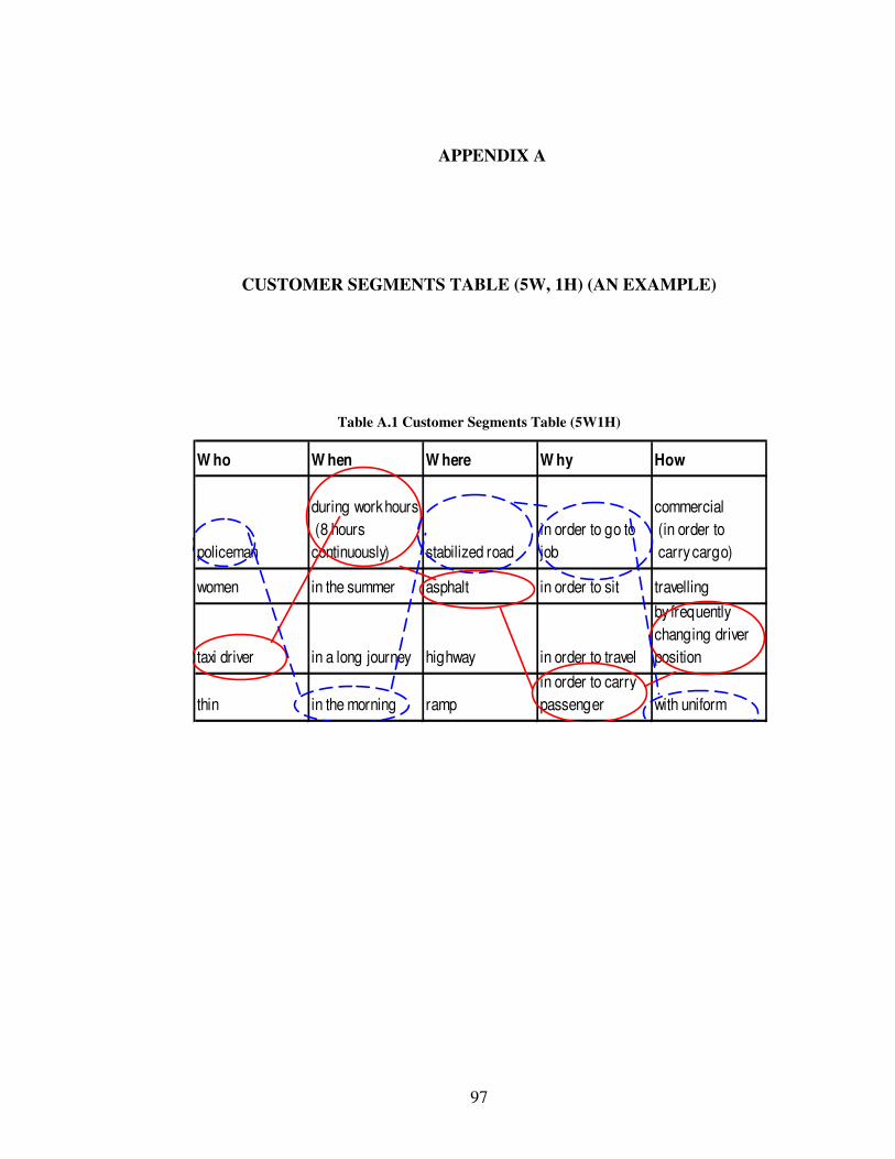
97

APPENDIX A

CUSTOMER SEGMENTS TABLE (5W, 1H) (AN EXAMPLE)

Table A.1 Customer Segments Table (5W1H)

W ho W hen W here W hy How

policeman

during work hours

(8 hours

continuously) stabilized road

in order to go to

job

commercial

(in order to

carry cargo)

women in the summer asphalt in order to sit travelling

taxi driver in a long journey highway in order to travel

by frequently

changing driver

position

thin in the morning ramp

in order to carry

passenger with uniform

98

APPENDIX B

THE QUESTIONNAIRE

CHAPTER I

Demographic questions are asked in this chapter.

Question1: Gender?

Man (1) Women (2)

Question2: Age?

18-20 (1) 21-25 (2) 26-30 (3) 31-35 (4) 36-40 (5) 41-45 (6) 46-50 (7) 51-55 (8) Greater then 55 (9)

Question3: Education level?

Primary (1) High school (2) Fore license (2 years) (3) University graduates (4)

Question4: Occupation?

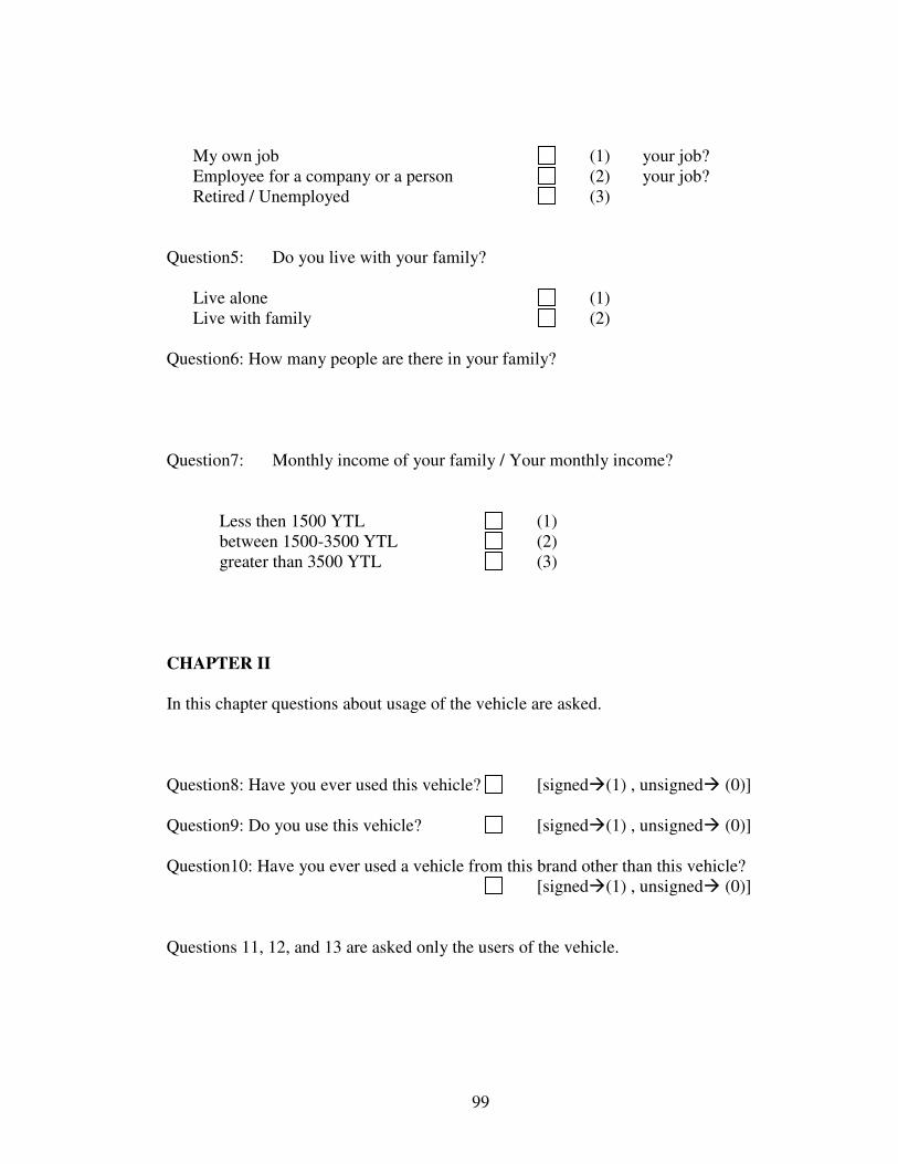
99

My own job (1) your job? Employee for a company or a person (2) your job? Retired / Unemployed (3)

Question5: Do you live with your family?

Live alone (1) Live with family (2)

Question6: How many people are there in your family?

Question7: Monthly income of your family / Your monthly income?

Less then 1500 YTL (1)

between 1500-3500 YTL (2) greater than 3500 YTL (3)

CHAPTER II

In this chapter questions about usage of the vehicle are asked.

Question8: Have you ever used this vehicle? [signed�(1) , unsigned� (0)] Question9: Do you use this vehicle? [signed�(1) , unsigned� (0)] Question10: Have you ever used a vehicle from this brand other than this vehicle?

[signed�(1) , unsigned� (0)]

Questions 11, 12, and 13 are asked only the users of the vehicle.

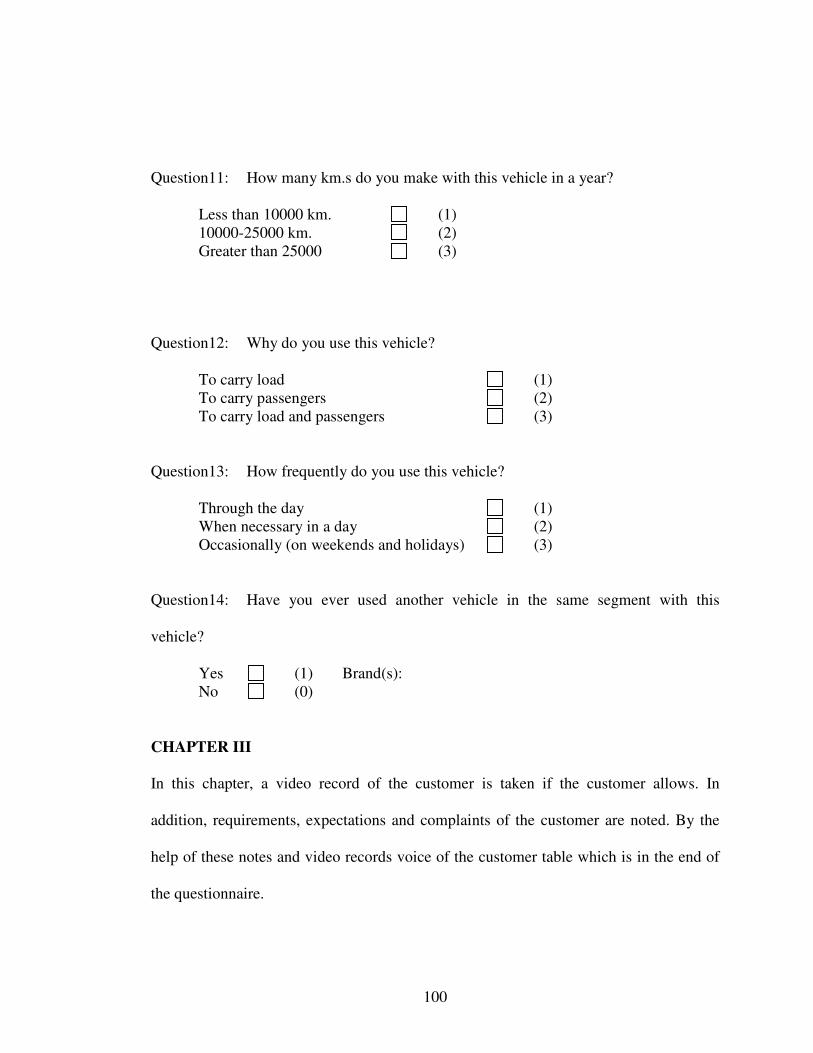
100

Question11: How many km.s do you make with this vehicle in a year?

Less than 10000 km. (1) 10000-25000 km. (2) Greater than 25000 (3)

Question12: Why do you use this vehicle?

To carry load (1) To carry passengers (2) To carry load and passengers (3)

Question13: How frequently do you use this vehicle?

Through the day (1) When necessary in a day (2) Occasionally (on weekends and holidays) (3)

Question14: Have you ever used another vehicle in the same segment with this

vehicle?

Yes (1) Brand(s): No (0)

CHAPTER III

In this chapter, a video record of the customer is taken if the customer allows. In

addition, requirements, expectations and complaints of the customer are noted. By the

help of these notes and video records voice of the customer table which is in the end of

the questionnaire.

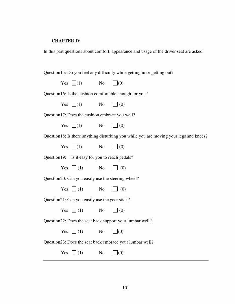
101

CHAPTER IV

In this part questions about comfort, appearance and usage of the driver seat are asked.

Question15: Do you feel any difficulty while getting in or getting out?

Yes (1) No (0)

Question16: Is the cushion comfortable enough for you?

Yes (1) No (0)

Question17: Does the cushion embrace you well?

Yes (1) No (0)

Question18: Is there anything disturbing you while you are moving your legs and knees?

Yes (1) No (0)

Question19: Is it easy for you to reach pedals?

Yes (1) No (0)

Question20: Can you easily use the steering wheel?

Yes (1) No (0)

Question21: Can you easily use the gear stick?

Yes (1) No (0)

Question22: Does the seat back support your lumbar well?

Yes (1) No (0)

Question23: Does the seat back embrace your lumbar well?

Yes (1) No (0)

102

Question24: Does the seat back support your back well?

Yes (1) No (0)

Question25: Does the seat back embrace your back well?

Yes (1) No (0)

What is your expectation from the head restraint?

Question26: Protect my head when a crash occurs? [Signed �(1), unsigned� (0)]

Question27: Rest my head? [Signed �(1), unsigned� (0)]

Question28: Does this head restraint meet your expectations?

Yes (1) No (0)

Question29: Is your forward visibility good?

Yes (1) No (0)

Question30: Is your backward visibility good?

Yes (1) No (0)

Can you easily access the seat adjustments? Yes No Which adjustments?

Question31: Access to fore-aft adjustment [signed�(1) , unsigned� (0)]

Question32: Access to vertical adjustment [signed�(1) , unsigned� (0)]

Question33: Access to back angle adjustment [signed�(1) , unsigned� (0)]

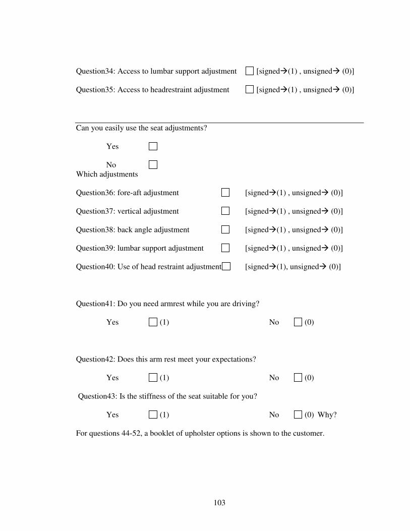
103

Question34: Access to lumbar support adjustment [signed�(1) , unsigned� (0)]

Question35: Access to headrestraint adjustment [signed�(1) , unsigned� (0)]

Can you easily use the seat adjustments?

Yes No Which adjustments

Question36: fore-aft adjustment [signed�(1) , unsigned� (0)]

Question37: vertical adjustment [signed�(1) , unsigned� (0)]

Question38: back angle adjustment [signed�(1) , unsigned� (0)]

Question39: lumbar support adjustment [signed�(1) , unsigned� (0)]

Question40: Use of head restraint adjustment [signed�(1), unsigned� (0)]

Question41: Do you need armrest while you are driving?

Yes (1) No (0)

Question42: Does this arm rest meet your expectations?

Yes (1) No (0)

Question43: Is the stiffness of the seat suitable for you?

Yes (1) No (0) Why?

For questions 44-52, a booklet of upholster options is shown to the customer.

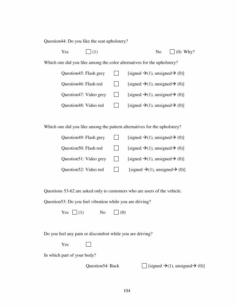
104

Question44: Do you like the seat upholstery?

Yes (1) No (0) Why?

Which one did you like among the color alternatives for the upholstery?

Question45: Flash grey [signed �(1), unsigned� (0)]

Question46: Flash red [signed �(1), unsigned� (0)]

Question47: Video grey [signed �(1), unsigned� (0)]

Question48: Video red [signed �(1), unsigned� (0)]

Which one did you like among the pattern alternatives for the upholstery?

Question49: Flash grey [signed �(1), unsigned� (0)]

Question50: Flash red [signed �(1), unsigned� (0)]

Question51: Video grey [signed �(1), unsigned� (0)]

Question52: Video red [signed �(1), unsigned� (0)]

Questions 53-62 are asked only to customers who are users of the vehicle.

Question53: Do you feel vibration while you are driving?

Yes (1) No (0)

Do you feel any pain or discomfort while you are driving?

Yes

In which part of your body?

Question54: Back [signed �(1), unsigned� (0)]

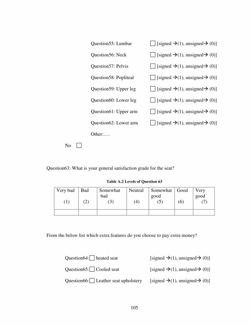
105

Question55: Lumbar [signed �(1), unsigned� (0)]

Question56: Neck [signed �(1), unsigned� (0)]

Question57: Pelvis [signed �(1), unsigned� (0)]

Question58: Popliteal [signed �(1), unsigned� (0)]

Question59: Upper leg [signed �(1), unsigned� (0)]

Question60: Lower leg [signed �(1), unsigned� (0)]

Question61: Upper arm [signed �(1), unsigned� (0)]

Question62: Lower arm [signed �(1), unsigned� (0)]

Other:….

No

Question63: What is your general satisfaction grade for the seat?

Table A.2 Levels of Question 63

From the below list which extra features do you choose to pay extra money?

Question64: heated seat [signed �(1), unsigned� (0)]

Question65: Cooled seat [signed �(1), unsigned� (0)]

Question66: Leather seat upholstery [signed �(1), unsigned� (0)]

Very bad (1)

Bad (2)

Somewhat bad (3)

Neutral (4)

Somewhat good (5)

Good (6)

Very good (7)

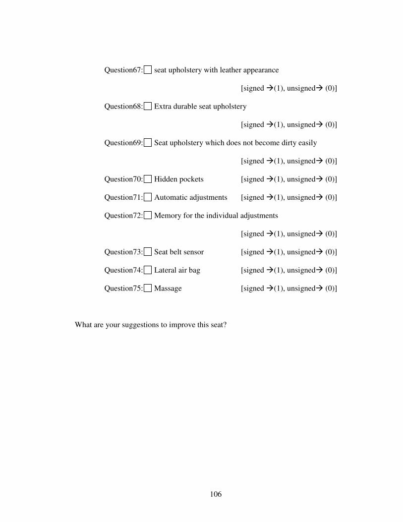
106

Question67: seat upholstery with leather appearance

[signed �(1), unsigned� (0)]

Question68: Extra durable seat upholstery

[signed �(1), unsigned� (0)]

Question69: Seat upholstery which does not become dirty easily

[signed �(1), unsigned� (0)]

Question70: Hidden pockets [signed �(1), unsigned� (0)]

Question71: Automatic adjustments [signed �(1), unsigned� (0)]

Question72: Memory for the individual adjustments

[signed �(1), unsigned� (0)]

Question73: Seat belt sensor [signed �(1), unsigned� (0)]

Question74: Lateral air bag [signed �(1), unsigned� (0)]

Question75: Massage [signed �(1), unsigned� (0)]

What are your suggestions to improve this seat?

107

CHAPTER V

In this part anthropometrical measures of customer are made using an anthropolometre.

Table A.3 Anthropometrical Measures

Body Measures

Measures

Question76: Weight

Question77: Height

Question78: Arm length

Question79: Fore arm length

Question80: Upper arm length

Question81: Hand length

Question82: Shoulder width

Question83: Hip width while sitting

Question84: Hip-knee length

Question85: Hip-popliteal length

Question86: Bust height while sitting

Question87: Eye height while sitting

Question88: Shoulder height while sitting

Question89: Knee height while sitting

108

Voice of the Customer Table

Table A.4 Voice of the Customer Table

WHO WHAT WHERE WHEN WHY HOW Improvement

opportunities

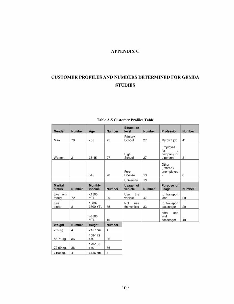
109

APPENDIX C

CUSTOMER PROFILES AND NUMBERS DETERMINED FOR GEMBA

STUDIES

Table A.5 Customer Profiles Table

Gender Number Age Number Education level Number Profession Number

Man 78 <35 25 Primary School 27 My own job 41

Women 2 36-45 27 High School 27

Employee for a company or a person 31

>45 28 Fore License 13

Other ( retired / unemployed ) 8

University 13

Marital status Number

Monthly income Number

Usage of vehicle Number

Purpose of usage Number

Live with family 72

<1500 YTL 29

Use the vehicle 47

to transport load 20

Live alone 8

1500-3500 YTL 35

Not use the vehicle 33

to transport passenger 20

>3500 YTL 16

both load and passenger 40

Weight Number Height Number

<55 kg. 4 <157 cm. 4

56-71 kg. 36 158-172 cm. 36

72-99 kg. 36 173-185 cm. 36

>100 kg. 4 >186 cm. 4

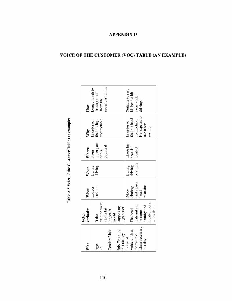
11

0

AP

PE

ND

IX D

CU

ST

OM

ER

(V

OC

) T

AB

LE

(A

N E

XA

MP

LE

)

Tab

le A

.5 V

oice

of

the

Cu

stom

er T

able

(an

exa

mp

le)

Wh

o V

OC

-ve

rbat

im

Wh

at

Wh

en

Wh

ere

Wh

y H

ow

If t

he

cush

ion

wer

e a

litt

le b

it

long

er, i

t w

ould

su

ppor

t m

y le

gs b

ette

r

Lon

ger

cush

ion

Dur

ing

driv

ing

Fro

m

uppe

r pa

rt

of h

is

popl

itea

l

In o

rder

to

feel

his

leg

co

mfo

rtab

le

Lon

g en

ough

to

be

supp

orte

d f

rom

the

up

per

part

of

his

popl

itea

l

Age

:

26

Gen

der:

Mal

e Jo

b: W

orki

ng

in a

fac

tory

U

sage

of

Veh

icle

: U

ses

the

vehi

cle

whe

n ne

cess

ary

in a

day

The

hea

d re

stra

int

can

be m

ore

chub

by a

nd

loca

ted

mor

e to

the

fro

nt

Mor

e ch

ubby

an

d cl

oser

he

ad

rest

rain

t

Dur

ing

driv

ing

or s

itti

ng

whe

re h

is

head

is

loca

ted

In o

rder

to

feel

his

hea

d co

mfo

rtab

le.

He

expe

cts

to

use

it f

or

rest

ing.

Sui

tabl

e to

res

t hi

s he

ad a

bit

ev

en w

hile

dr

ivin

g.

APPENDIX D

VOICE OF THE CUSTOMER (VOC) TABLE (AN EXAMPLE)

110

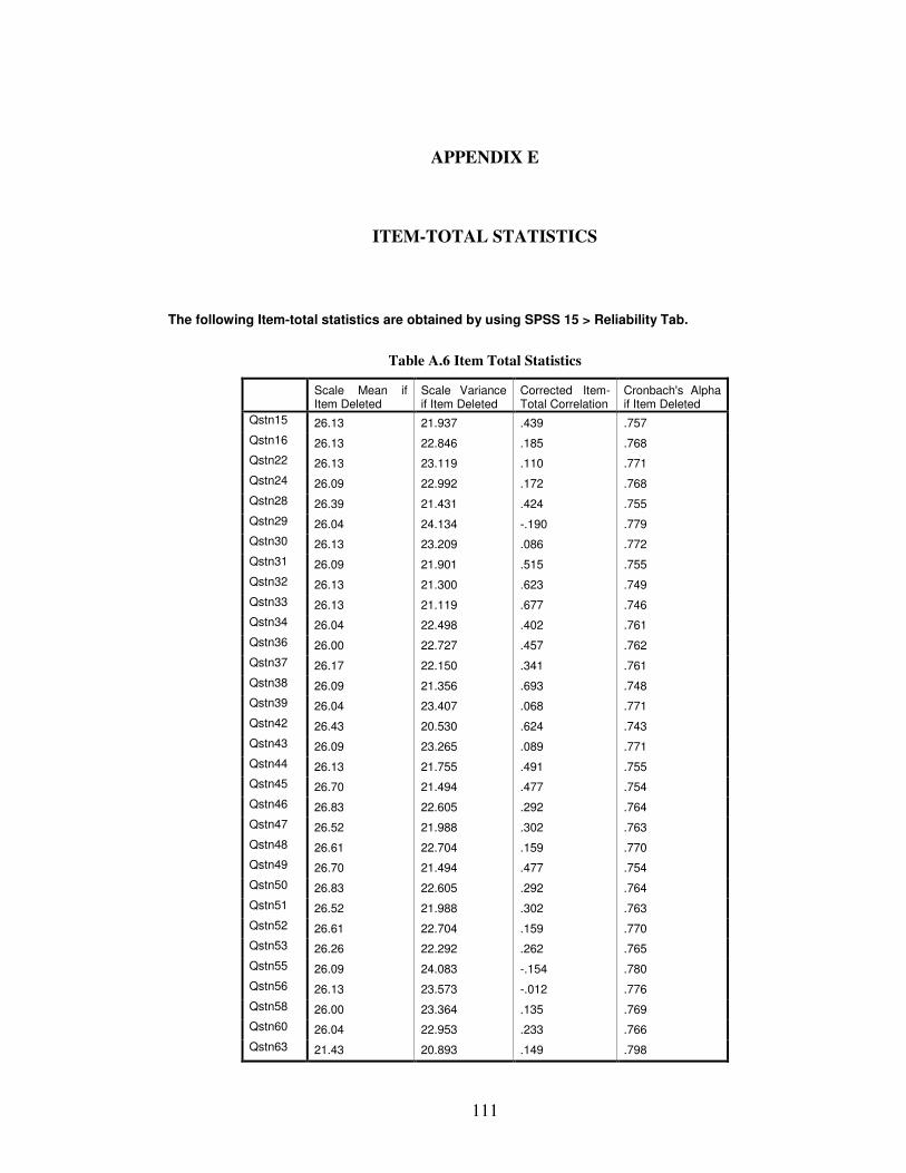
111

APPENDIX E

ITEM-TOTAL STATISTICS

The following Item-total statistics are obtained by using SPSS 15 > Reliability Tab.

Table A.6 Item Total Statistics

Scale Mean if Item Deleted

Scale Variance if Item Deleted

Corrected Item-Total Correlation

Cronbach's Alpha if Item Deleted

Qstn15 26.13 21.937 .439 .757

Qstn16 26.13 22.846 .185 .768

Qstn22 26.13 23.119 .110 .771

Qstn24 26.09 22.992 .172 .768

Qstn28 26.39 21.431 .424 .755

Qstn29 26.04 24.134 -.190 .779

Qstn30 26.13 23.209 .086 .772

Qstn31 26.09 21.901 .515 .755

Qstn32 26.13 21.300 .623 .749

Qstn33 26.13 21.119 .677 .746

Qstn34 26.04 22.498 .402 .761

Qstn36 26.00 22.727 .457 .762

Qstn37 26.17 22.150 .341 .761

Qstn38 26.09 21.356 .693 .748

Qstn39 26.04 23.407 .068 .771

Qstn42 26.43 20.530 .624 .743

Qstn43 26.09 23.265 .089 .771

Qstn44 26.13 21.755 .491 .755

Qstn45 26.70 21.494 .477 .754

Qstn46 26.83 22.605 .292 .764

Qstn47 26.52 21.988 .302 .763

Qstn48 26.61 22.704 .159 .770

Qstn49 26.70 21.494 .477 .754

Qstn50 26.83 22.605 .292 .764

Qstn51 26.52 21.988 .302 .763

Qstn52 26.61 22.704 .159 .770

Qstn53 26.26 22.292 .262 .765

Qstn55 26.09 24.083 -.154 .780

Qstn56 26.13 23.573 -.012 .776

Qstn58 26.00 23.364 .135 .769

Qstn60 26.04 22.953 .233 .766

Qstn63 21.43 20.893 .149 .798

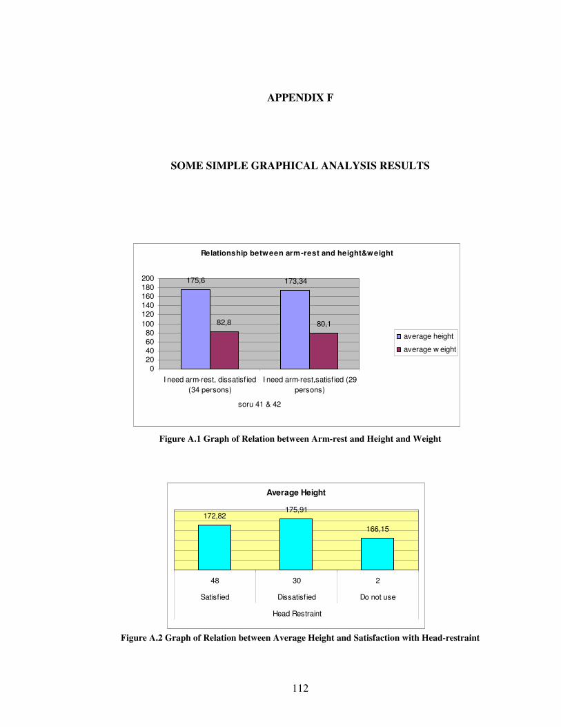
112

APPENDIX F

SOME SIMPLE GRAPHICAL ANALYSIS RESULTS

Figure A.1 Graph of Relation between Arm-rest and Height and Weight

Figure A.2 Graph of Relation between Average Height and Satisfaction with Head-restraint

Relationship between arm-rest and height&weight

175,6 173,34

82,8 80,1

020406080

100

120140160180200

I need arm-rest, dissatisf ied

(34 persons)

I need arm-rest,satisf ied (29

persons)

soru 41 & 42

average height

average w eight

Average Height

172,82175,91

166,15

48 30 2

Satisf ied Dissatisf ied Do not use

Head Restraint

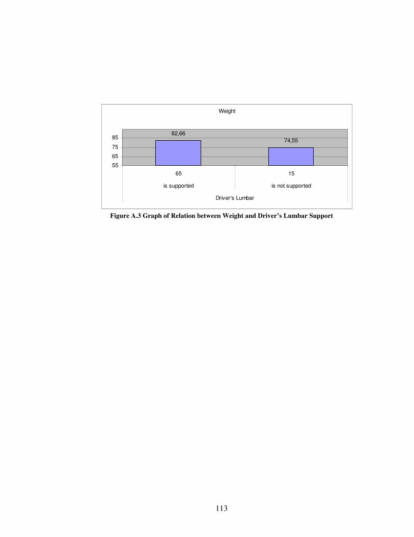
113

Figure A.3 Graph of Relation between Weight and Driver’s Lumbar Support

Weight

82,66

74,55

55

65

75

85

65 15

is supported is not supported

Driver's Lumbar

114

APPENDIX G

CORRELATION MATRIX

Correlation matrix is formed by Minitab 15. In this matrix, correlations between

questions asked every participant are concerned. In this appendix only the lines

including significant correlation values are shown. (Correlation values grater than 0.5

are marked.)

Cell Contents: Pearson correlation P-Value

Table A.7 Correlation Matrix

Qstn8_1 Qstn10 Qstn11 Qstn12 Qstn13 Qstn14

Qstn11 0.846 -0.236

0.000 0.035

Qstn12 0.894 -0.140 0.716

0.000 0.217 0.000

Qstn13 0.863 -0.087 0.615 0.777

0.000 0.442 0.000 0.000

Qstn29 Qstn30 Qstn31 Qstn32 Qstn33

Qstn33 -0.017 0.068 0.287 0.629

0.884 0.549 0.010 0.000

Qstn34 0.048 0.010 0.161 0.537 0.486

0.677 0.927 0.157 0.000 0.000

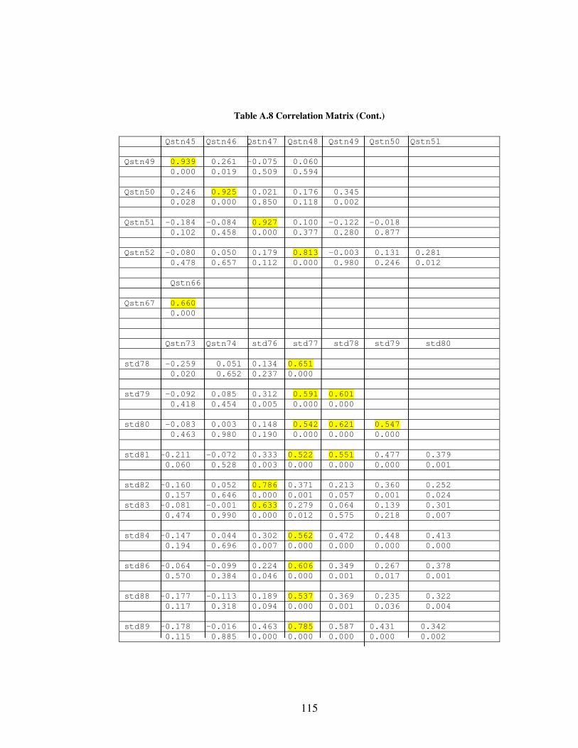
115

Table A.8 Correlation Matrix (Cont.)

Qstn45 Qstn46 Qstn47 Qstn48 Qstn49 Qstn50 Qstn51

Qstn49 0.939 0.261 -0.075 0.060

0.000 0.019 0.509 0.594

Qstn50 0.246 0.925 0.021 0.176 0.345

0.028 0.000 0.850 0.118 0.002

Qstn51 -0.184 -0.084 0.927 0.100 -0.122 -0.018

0.102 0.458 0.000 0.377 0.280 0.877

Qstn52 -0.080 0.050 0.179 0.813 -0.003 0.131 0.281

0.478 0.657 0.112 0.000 0.980 0.246 0.012

Qstn66

Qstn67 0.660

0.000

Qstn73 Qstn74 std76 std77 std78 std79 std80

std78 -0.259 0.051 0.134 0.651

0.020 0.652 0.237 0.000

std79 -0.092 0.085 0.312 0.591 0.601

0.418 0.454 0.005 0.000 0.000

std80 -0.083 0.003 0.148 0.542 0.621 0.547

0.463 0.980 0.190 0.000 0.000 0.000

std81 -0.211 -0.072 0.333 0.522 0.551 0.477 0.379

0.060 0.528 0.003 0.000 0.000 0.000 0.001

std82 -0.160 0.052 0.786 0.371 0.213 0.360 0.252

0.157 0.646 0.000 0.001 0.057 0.001 0.024

std83 -0.081 -0.001 0.633 0.279 0.064 0.139 0.301

0.474 0.990 0.000 0.012 0.575 0.218 0.007

std84 -0.147 0.044 0.302 0.562 0.472 0.448 0.413

0.194 0.696 0.007 0.000 0.000 0.000 0.000

std86 -0.064 -0.099 0.224 0.606 0.349 0.267 0.378

0.570 0.384 0.046 0.000 0.001 0.017 0.001

std88 -0.177 -0.113 0.189 0.537 0.369 0.235 0.322

0.117 0.318 0.094 0.000 0.001 0.036 0.004

std89 -0.178 -0.016 0.463 0.785 0.587 0.431 0.342

0.115 0.885 0.000 0.000 0.000 0.000 0.002

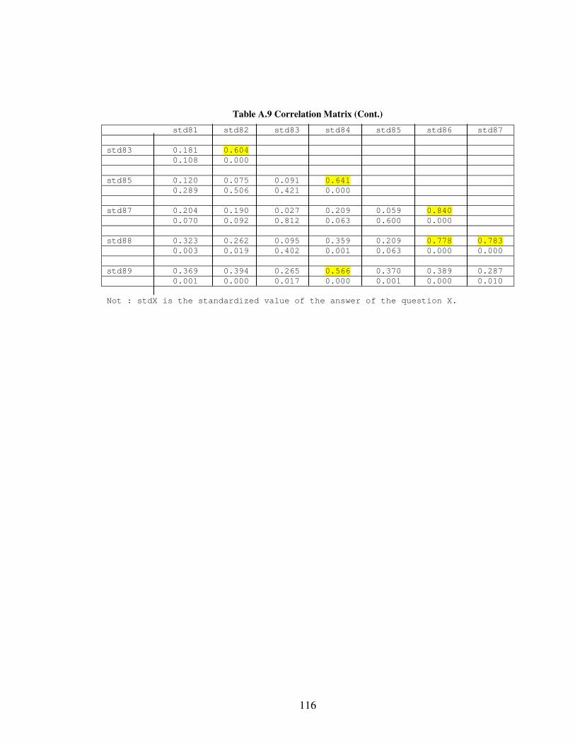
116

Table A.9 Correlation Matrix (Cont.)

std81 std82 std83 std84 std85 std86 std87

std83 0.181 0.604

0.108 0.000

std85 0.120 0.075 0.091 0.641

0.289 0.506 0.421 0.000

std87 0.204 0.190 0.027 0.209 0.059 0.840

0.070 0.092 0.812 0.063 0.600 0.000

std88 0.323 0.262 0.095 0.359 0.209 0.778 0.783

0.003 0.019 0.402 0.001 0.063 0.000 0.000

std89 0.369 0.394 0.265 0.566 0.370 0.389 0.287

0.001 0.000 0.017 0.000 0.001 0.000 0.010

Not : stdX is the standardized value of the answer of the question X.

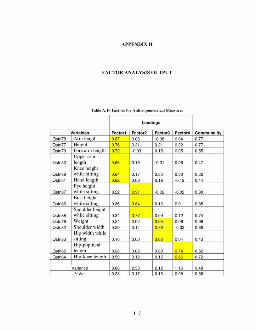
117

APPENDIX H

FACTOR ANALYSIS OUTPUT

Table A.10 Factors for Anthropometrical Measures

Loadings

Variables Factor1 Factor2 Factor3 Factor4 Communality

Qstn78 Arm length 0.87 0.08 -0.08 0.04 0.77

Qstn77 Height 0.76 0.31 0.21 0.22 0.77

Qstn79 Fore arm length 0.72 -0.03 0.15 0.05 0.55

Qstn80

Upper arm length 0.66 0.16 -0.01 0.06 0.47

Qstn89

Knee height while sitting 0.64 0.17 0.30 0.30 0.62

Qstn81 Hand length 0.62 0.08 0.19 -0.12 0.44

Qstn87

Eye height while sitting 0.22 0.91 -0.02 -0.02 0.88

Qstn86

Bust height while sitting 0.36 0.84 0.13 0.01 0.85

Qstn88

Shoulder height while sitting 0.34 0.77 0.09 0.12 0.74

Qstn76 Weight 0.24 0.02 0.95 0.06 0.96

Qstn82 Shoulder width 0.29 0.14 0.76 -0.03 0.68

Qstn83

Hip width while sitting 0.16 0.00 0.63 0.04 0.43

Qstn85

Hip-popliteal length 0.28 0.02 0.00 0.74 0.62

Qstn84 Hip-knee length 0.50 0.12 0.15 0.66 0.72

Variance 3.88 2.33 2.12 1.16 9.49

%Var 0.28 0.17 0.15 0.08 0.68

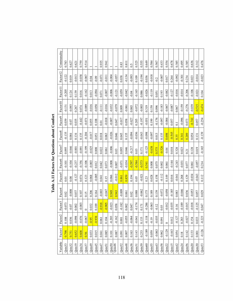
11

8

1)

Fac

tor

anal

yses

ou

tpu

t fo

r d

iscr

ete

qu

esti

ons

wh

ich

can

be

trea

ted

as

con

tin

uou

s va

riab

le

Tab

le A

.11

Fac

tors

for

Qu

esti

ons

abou

t C

omfo

rt

Var

iabl

e F

acto

r1

Fac

tor2

F

acto

r3

Fac

tor4

F

acto

r5

Fac

tor6

F

acto

r7

Fac

tor8

F

acto

r9

Fac

tor1

0 F

acto

r11

Fac

tor1

2 C

omm

unal

ity

Qst

n33

0.79

8 0.

108

-0.0

73

0.02

0.

01

-0.1

01

0.09

5 -0

.135

0.

039

-0.1

31

-0.2

05

-0.1

22

0.78

3

Qst

n32

0.75

1 0.

036

-0.0

7 -0

.008

0.

08

-0.1

04

-0.0

46

0.08

4 -0

.07

-0.0

93

0.12

4 0.

019

0.62

7

Qst

n19

0.65

2 -0

.098

0.

002

0.03

7 -0

.127

-0

.237

-0

.001

0.

134

0.03

5 0.

267

0.13

9 -0

.013

0.

621

Qst

n34

0.60

8 -0

.076

-0

.003

0.

107

0.07

4 -0

.356

-0

.091

0.

135

-0.4

42

0.07

4 0.

016

-0.0

38

0.75

9

Qst

n37

0.56

-0

.067

0

0.15

0.

123

-0.1

06

-0.1

99

-0.2

04

-0.0

71

-0.0

89

-0.1

62

-0.0

67

0.51

4

Qst

n49

0.03

3 -0

.95

0.03

2 0.

206

0.06

8 -0

.003

-0

.025

-0

.017

0.

055

-0.0

16

0.01

3 -0

.04

1

Qst

n45

0.01

5 -0

.938

0.

109

0.16

4 -0

.005

0.

012

0.00

8 0.

051

0.10

8 -0

.058

-0

.094

-0

.09

1

Qst

n47

0.04

1 0.

061

-0.9

18

-0.0

03

0.04

1 0.

042

0.02

2 0.

018

0.01

-0

.111

0.

071

-0.0

71

0.93

5

Qst

n51

0.08

5 0.

104

-0.9

05

-0.0

47

0.15

0.

073

0.06

1 0.

063

-0.0

18

-0.0

16

-0.0

07

-0.0

11

0.94

1

Qst

n50

0.10

1 -0

.203

-0

.023

0.

949

0.06

6 -0

.008

-0

.006

-0

.026

-0

.007

-0

.032

-0

.006

-0

.004

1

Qst

n46

0.08

7 -0

.162

0.

058

0.94

3 -0

.012

0.

007

0.03

0.

046

0.04

7 -0

.079

-0

.121

-0

.057

1

Qst

n52

0.09

1 0.

001

-0.1

82

-0.0

09

0.86

1 -0

.071

0.

095

0.04

5 -0

.017

0.

009

-0.0

59

0.03

8 0.

83

Qst

n48

0.00

7 -0

.055

0.

002

0.06

1 0.

859

-0.0

34

0.04

6 0.

135

0.05

8 -0

.061

-0

.042

-0

.134

0.

811

Qst

n36

0.16

3 -0

.064

0.

047

0.02

0.

194

-0.5

97

-0.2

17

-0.0

94

-0.0

27

0.06

5 -0

.04

-0.0

93

0.5

Qst

n31

0.14

3 -0

.041

-0

.174

0.

088

0.05

-0

.584

0.

03

-0.0

36

0.20

5 -0

.072

-0

.165

0.

109

0.52

5

Qst

n39

0.23

3 0.

133

0.17

1 -0

.062

-0

.021

-0

.573

0.

171

-0.0

43

-0.1

97

-0.0

03

0.08

6 -0

.194

0.

555

Qst

n60

-0.1

89

-0.1

18

-0.2

86

0.17

5 0.

23

0.54

1 -0

.125

-0

.098

-0

.051

0.

319

-0.0

26

0.03

6 0.

649

Qst

n55

0.05

9 -0

.19

-0.0

63

0.18

9 0.

028

0.00

8 -0

.638

-0

.097

0.

199

0.15

9 -0

.119

-0

.018

0.

584

Qst

n43

-0.0

63

-0.0

35

-0.1

2 0.

139

0.15

8 0.

075

0.57

5 0.

013

-0.1

76

0.09

6 0.

051

-0.2

0.

567

Qst

n58

0.06

2 0.

091

0.03

-0

.072

-0

.112

0.

002

-0.5

26

0.13

5 -0

.097

-0

.183

0.

193

-0.0

07

0.43

3

Qst

n22

-0.1

29

0 -0

.012

-0

.058

0.

149

0.06

1 -0

.04

0.69

8 -0

.084

-0

.067

-0

.082

0.

017

0.55

4

Qst

n15

-0.4

43

0.01

2 -0

.035

-0

.185

0.

016

-0.1

44

0.01

8 -0

.545

0.

057

-0.0

87

-0.1

27

0.26

4 0.

678

Qst

n42

0.05

4 -0

.127

-0

.16

0.08

3 -0

.041

-0

.243

0.

328

0.35

0.

1 0.

067

-0.0

16

-0.0

92

0.38

5

Qst

n24

0.18

0.

283

-0.1

89

-0.0

46

0.26

8 -0

.031

0.

023

0.34

1 -0

.096

-0

.159

-0

.014

-0

.301

0.

495

Qst

n56

0.14

2 -0

.027

-0

.015

0.

036

0.12

9 0.

077

0.21

0.

289

0.07

3 -0

.276

-0

.206

0.

234

0.38

5

Qst

n20

0.13

3 0.

154

-0.0

18

-0.0

53

-0.0

34

0.06

1 0.

128

0.05

4 -0

.741

-0

.039

-0

.106

0.

023

0.63

6

Qst

n30

0.00

1 0.

033

-0.1

25

0.05

7 -0

.043

-0

.057

0.

019

0.13

1 0.

057

-0.5

15

-0.0

21

-0.0

14

0.31

2

Qst

n53

-0.1

26

-0.2

23

0.04

7 0.

029

0.11

2 0.

214

-0.1

65

-0.1

39

-0.2

54

-0.4

74

0.10

4 -0

.023

0.

476

118

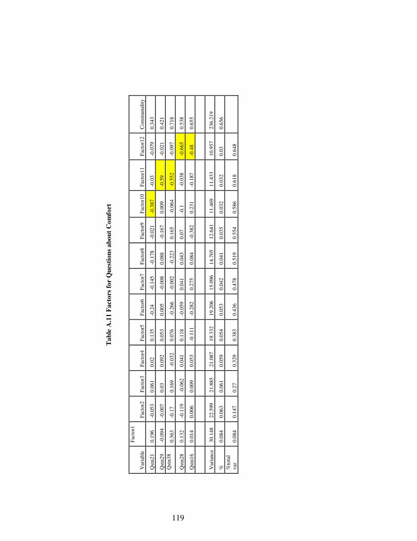
11

9

Var

iabl

e

Fac

tor1

Fac

tor2

F

acto

r3

Fac

tor4

F

acto

r5

Fac

tor6

F

acto

r7

Fac

tor8

F

acto

r9

Fac

tor1

0 F

acto

r11

Fac

tor1

2 C

omm

unal

ity

Qst

n21

0.19

6 -0

.053

0.

061

0.02

0.

135

-0.2

4 -0

.145

-0

.178

-0

.021

-0

.387

-0

.03

-0.0

79

0.34

3

Qst

n29

-0.0

94

-0.0

07

0.03

0.

092

0.05

3 0.

005

-0.0

08

0.08

8 -0

.167

0.

009

-0.5

9 -0

.021

0.

421

Qst

n38

0.36

3 -0

.17

0.16

9 -0

.032

0.

076

-0.2

66

-0.0

02

-0.2

23

0.16

5 -0

.064

-0

.552

-0

.097

0.

718

Qst

n28

0.13

2 -0

.119

-0

.062

0.

041

0.11

8 -0

.059

0.

041

0.04

3 0.

07

-0.1

-0

.038

-0

.665

0.

538

Qst

n16

0.01

4 0.

006

0.00

9 0.

053

-0.1

11

-0.2

82

0.27

5 0.

084

-0.3

82

0.23

1 -0

.187

-0

.48

0.65

5

Var

ianc

e 30

.148

22

.599

21

.885

21

.087

19

.332

19

.206

15

.096

14

.705

12

.641

11

.469

11

.433

10

.957

23

6.21

9

%

0.08

4 0.

063

0.06

1 0.

059

0.05

4 0.

053

0.04

2 0.

041

0.03

5 0.

032

0.03

2 0.

03

0.65

6 %

tota

l va

r 0.

084

0.14

7 0.

27

0.32

9 0.

383

0.43

6 0.

478

0.51

9 0.

554

0.58

6 0.

618

0.64

8

119

Tab

le A

.11

Fac

tors

for

Qu

esti

ons

abou

t C

omfo

rt

120

APPENDIX I

PRINCIPLE COMPONENT ANALYSIS OUTPUT

Principle component analysis is applied using Minitab 15.

Table A.12 Eigenanalysis of the Correlation Matrix

Eigenvalue 5.7743 2.0345 1.6906 1.1801 0.7536 0.5605 0.5292 0.3372

Proportion 0.412 0.145 0.121 0.084 0.054 0.040 0.038 0.024

Cumulative 0.412 0.558 0.679 0.763 0.817 0.857 0.894 0.919

Eigenvalue 0.2946 0.2437 0.1999 0.1661 0.1453 0.0903

Proportion 0.021 0.017 0.014 0.012 0.010 0.006

Cumulative 0.940 0.957 0.971 0.983 0.994 1.000

Table A.13 Principle Components for Anthropometrical Measures

Variable PC1 PC2 PC3 PC4

Qstn76 0.224 -0.465 -0.271 -0.069

Qstn77 0.368 0.037 0.081 0.006

Qstn78 0.301 0.094 0.304 0.292

Qstn79 0.277 -0.093 0.267 0.308

Qstn80 0.276 0.037 0.180 0.232

Qstn81 0.252 -0.042 0.077 0.437

Qstn82 0.238 -0.386 -0.323 0.012

Qstn83 0.166 -0.447 -0.266 -0.071

Qstn84 0.280 -0.025 0.282 -0.421

Qstn85 0.177 -0.006 0.358 -0.590

Qstn86 0.287 0.330 -0.335 -0.033

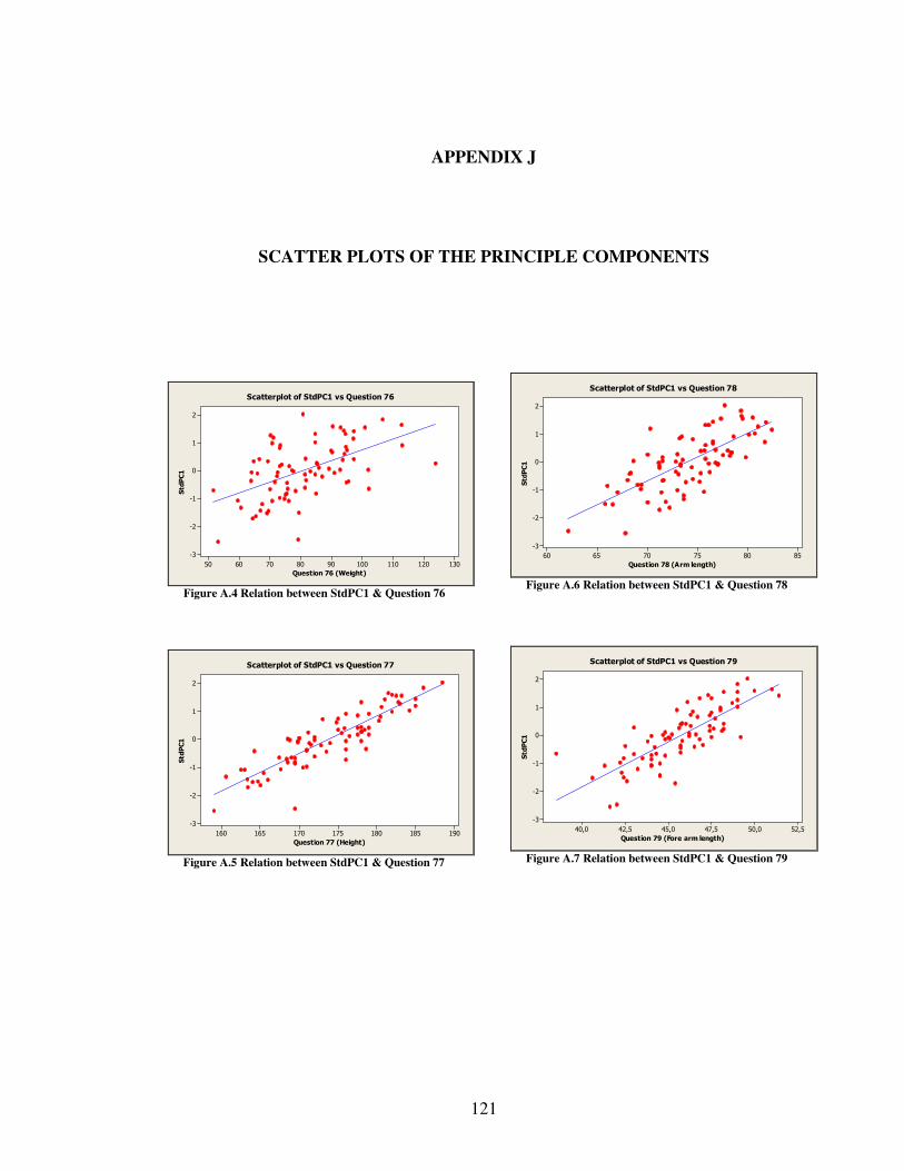
121

APPENDIX J

SCATTER PLOTS OF THE PRINCIPLE COMPONENTS

1301201101009080706050

2

1

0

-1

-2

-3

Question 76 (Weight)

StdPC1

Scatterplot of StdPC1 vs Question 76

Figure A.4 Relation between StdPC1 & Question 76

190185180175170165160

2

1

0

-1

-2

-3

Question 77 (Height)

StdPC1

Scatterplot of StdPC1 vs Question 77

Figure A.5 Relation between StdPC1 & Question 77

858075706560

2

1

0

-1

-2

-3

Question 78 (Arm length)

StdPC1

Scatterplot of StdPC1 vs Question 78

Figure A.6 Relation between StdPC1 & Question 78

52,550,047,545,042,540,0

2

1

0

-1

-2

-3

Question 79 (Fore arm length)

StdPC1

Scatterplot of StdPC1 vs Question 79

Figure A.7 Relation between StdPC1 & Question 79

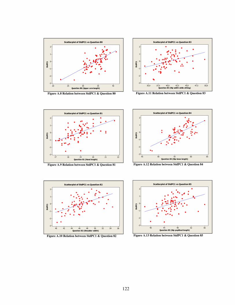
122

4035302520

2

1

0

-1

-2

-3

Question 80 (Upper arm length)

StdPC1

Scatterplot of StdPC1 vs Question 80

Figure A.8 Relation between StdPC1 & Question 80

222120191817

2

1

0

-1

-2

-3

Question 81 (Hand length)

StdPC1

Scatterplot of StdPC1 vs Question 81

Figure A.9 Relation between StdPC1 & Question 81

565452504846444240

2

1

0

-1

-2

-3

Question 82 (Shoulder width)

StdPC1

Scatterplot of StdPC1 vs Question 82

Figure A.10 Relation between StdPC1 & Question 82

50,047,545,042,540,037,535,0

2

1

0

-1

-2

-3

Question 83 (Hip width while sitting)

StdPC1

Scatterplot of StdPC1 vs Question 83

Figure A.11 Relation between StdPC1 & Question 83

6560555045

2

1

0

-1

-2

-3

Question 84 (Hip-knee length)

StdPC1

Scatterplot of StdPC1 vs Question 84

Figure A.12 Relation between StdPC1 & Question 84

5652484440

2

1

0

-1

-2

-3

Question 85 (Hip-popliteal length)

StdPC1

Scatterplot of StdPC1 vs Question 85

Figure A.13 Relation between StdPC1 & Question 85

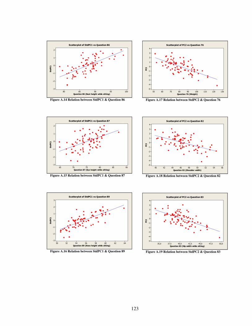
123

10095908580

2

1

0

-1

-2

-3

Question 86 (Bust height while sitting)

StdPC1

Scatterplot of StdPC1 vs Question 86

Figure A.14 Relation between StdPC1 & Question 86

908580757065

2

1

0

-1

-2

-3

Question 87 (Eye height while sitting)

StdPC1

Scatterplot of StdPC1 vs Question 87

Figure A.15 Relation between StdPC1 & Question 87

6462605856545250

3

2

1

0

-1

-2

-3

Question 89 (Knee height while sitting)

StdPC1

Scatterplot of StdPC1 vs Question 89

Figure A.16 Relation between StdPC1 & Question 89

1301201101009080706050

4

3

2

1

0

-1

-2

-3

-4

-5

Question 76 (Weight)

PC2

Scatterplot of PC2 vs Question 76

Figure A.17 Relation between StdPC2 & Question 76

565452504846444240

4

3

2

1

0

-1

-2

-3

-4

-5

Question 82 (Shoulder width)

PC2

Scatterplot of PC2 vs Question 82

Figure A.18 Relation between StdPC2 & Question 82

50,047,545,042,540,037,535,0

4

3

2

1

0

-1

-2

-3

-4

-5

Question 83 (Hip width while sitting)

PC2

Scatterplot of PC2 vs Question 83

Figure A.19 Relation between StdPC2 & Question 83

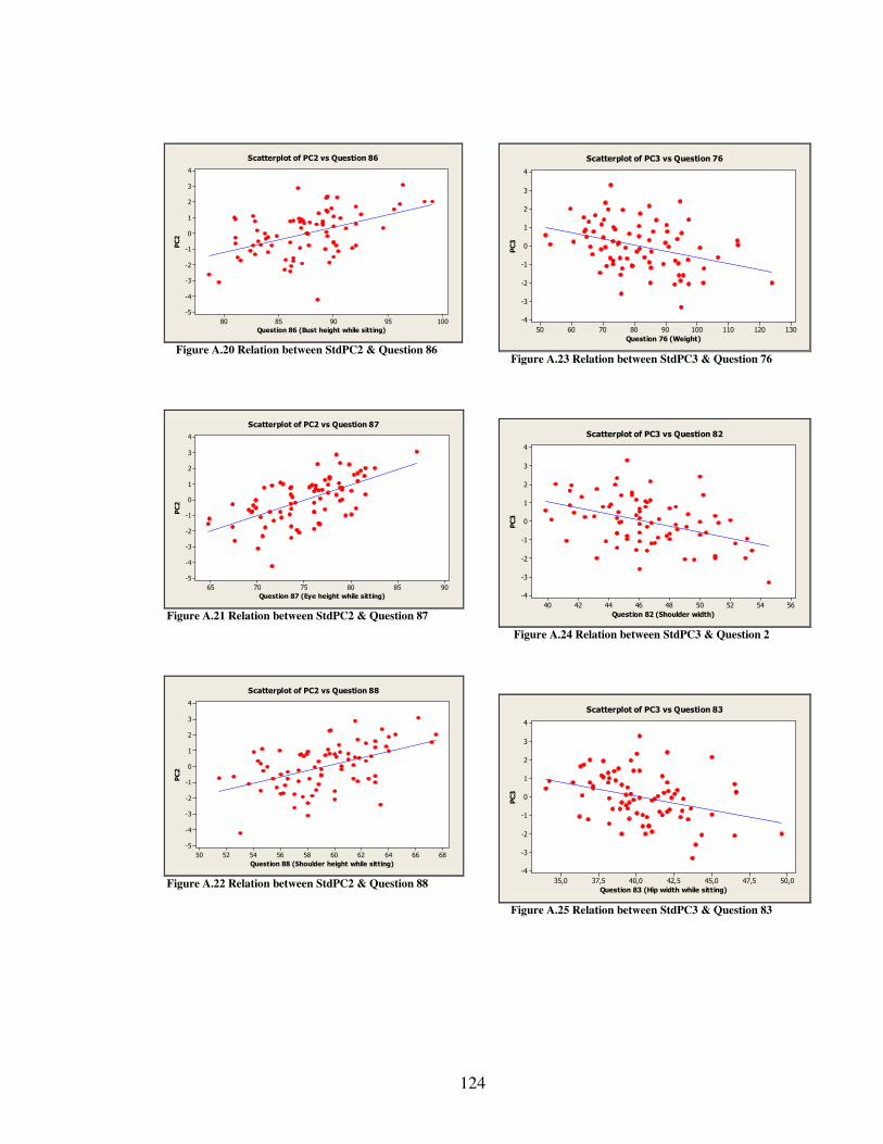
124

10095908580

4

3

2

1

0

-1

-2

-3

-4

-5

Question 86 (Bust height while sitting)

PC2

Scatterplot of PC2 vs Question 86

Figure A.20 Relation between StdPC2 & Question 86

908580757065

4

3

2

1

0

-1

-2

-3

-4

-5

Question 87 (Eye height while sitting)

PC2

Scatterplot of PC2 vs Question 87

Figure A.21 Relation between StdPC2 & Question 87

68666462605856545250

4

3

2

1

0

-1

-2

-3

-4

-5

Question 88 (Shoulder height while sitting)

PC2

Scatterplot of PC2 vs Question 88

Figure A.22 Relation between StdPC2 & Question 88

1301201101009080706050

4

3

2

1

0

-1

-2

-3

-4

Question 76 (Weight)

PC3

Scatterplot of PC3 vs Question 76

Figure A.23 Relation between StdPC3 & Question 76

565452504846444240

4

3

2

1

0

-1

-2

-3

-4

Question 82 (Shoulder width)

PC3

Scatterplot of PC3 vs Question 82

Figure A.24 Relation between StdPC3 & Question 2

50,047,545,042,540,037,535,0

4

3

2

1

0

-1

-2

-3

-4

Question 83 (Hip width while sitting)

PC3

Scatterplot of PC3 vs Question 83

Figure A.25 Relation between StdPC3 & Question 83

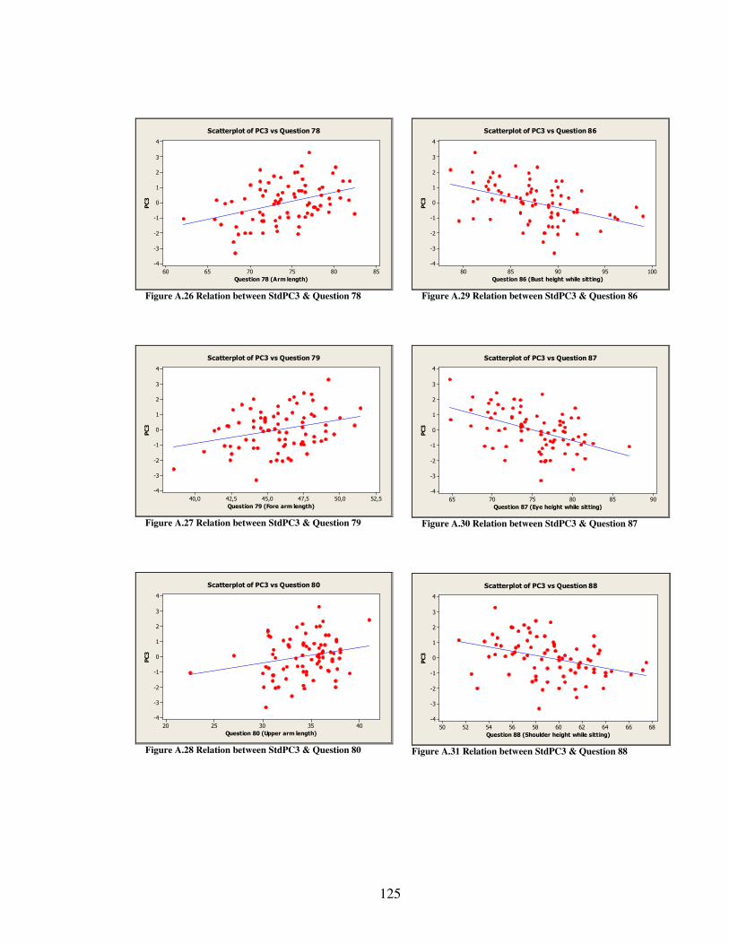
125

858075706560

4

3

2

1

0

-1

-2

-3

-4

Question 78 (Arm length)

PC3

Scatterplot of PC3 vs Question 78

Figure A.26 Relation between StdPC3 & Question 78

52,550,047,545,042,540,0

4

3

2

1

0

-1

-2

-3

-4

Question 79 (Fore arm length)

PC3

Scatterplot of PC3 vs Question 79

Figure A.27 Relation between StdPC3 & Question 79

4035302520

4

3

2

1

0

-1

-2

-3

-4

Question 80 (Upper arm length)

PC3

Scatterplot of PC3 vs Question 80

Figure A.28 Relation between StdPC3 & Question 80

10095908580

4

3

2

1

0

-1

-2

-3

-4

Question 86 (Bust height while sitting)

PC3

Scatterplot of PC3 vs Question 86

Figure A.29 Relation between StdPC3 & Question 86

908580757065

4

3

2

1

0

-1

-2

-3

-4

Question 87 (Eye height while sitting)

PC3

Scatterplot of PC3 vs Question 87

Figure A.30 Relation between StdPC3 & Question 87

68666462605856545250

4

3

2

1

0

-1

-2

-3

-4

Question 88 (Shoulder height while sitting)

PC3

Scatterplot of PC3 vs Question 88

Figure A.31 Relation between StdPC3 & Question 88

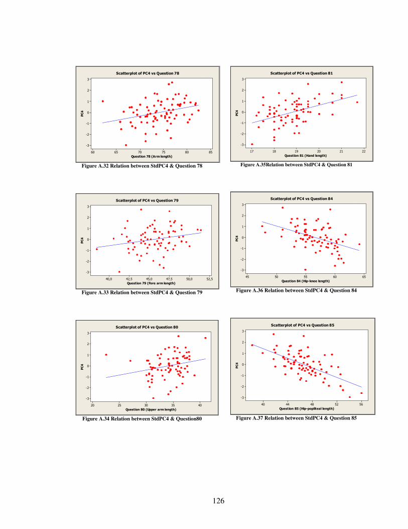
126

858075706560

3

2

1

0

-1

-2

-3

Question 78 (Arm length)

PC4

Scatterplot of PC4 vs Question 78

Figure A.32 Relation between StdPC4 & Question 78

52,550,047,545,042,540,0

3

2

1

0

-1

-2

-3

Question 79 (Fore arm length)

PC4

Scatterplot of PC4 vs Question 79

Figure A.33 Relation between StdPC4 & Question 79

4035302520

3

2

1

0

-1

-2

-3

Question 80 (Upper arm length)

PC4

Scatterplot of PC4 vs Question 80

Figure A.34 Relation between StdPC4 & Question80

222120191817

3

2

1

0

-1

-2

-3

Question 81 (Hand length)

PC4

Scatterplot of PC4 vs Question 81

Figure A.35Relation between StdPC4 & Question 81

6560555045

3

2

1

0

-1

-2

-3

Question 84 (Hip-knee length)

PC4

Scatterplot of PC4 vs Question 84

Figure A.36 Relation between StdPC4 & Question 84

5652484440

3

2

1

0

-1

-2

-3

Question 85 (Hip-popliteal length)

PC4

Scatterplot of PC4 vs Question 85

Figure A.37 Relation between StdPC4 & Question 85

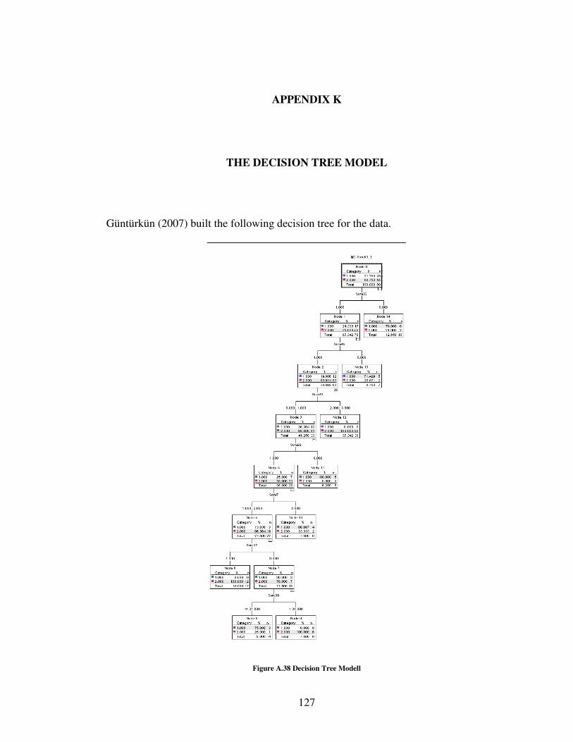
127

APPENDIX K

THE DECISION TREE MODEL

Güntürkün (2007) built the following decision tree for the data.

Figure A.38 Decision Tree Modell

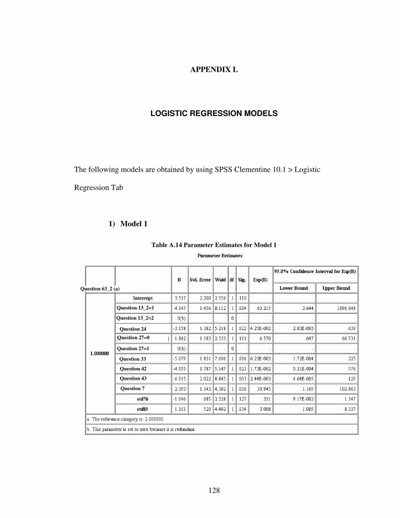
128

APPENDIX L

LOGISTIC REGRESSION MODELS

The following models are obtained by using SPSS Clementine 10.1 > Logistic

Regression Tab

1) Model 1

Table A.14 Parameter Estimates for Model 1

Question 24

Question 27=0

Question 27=1

Question 33

Question 42

Question 43

Question 7

Question 13_2=1

Question 13_2=2

Question 63_2 (a)

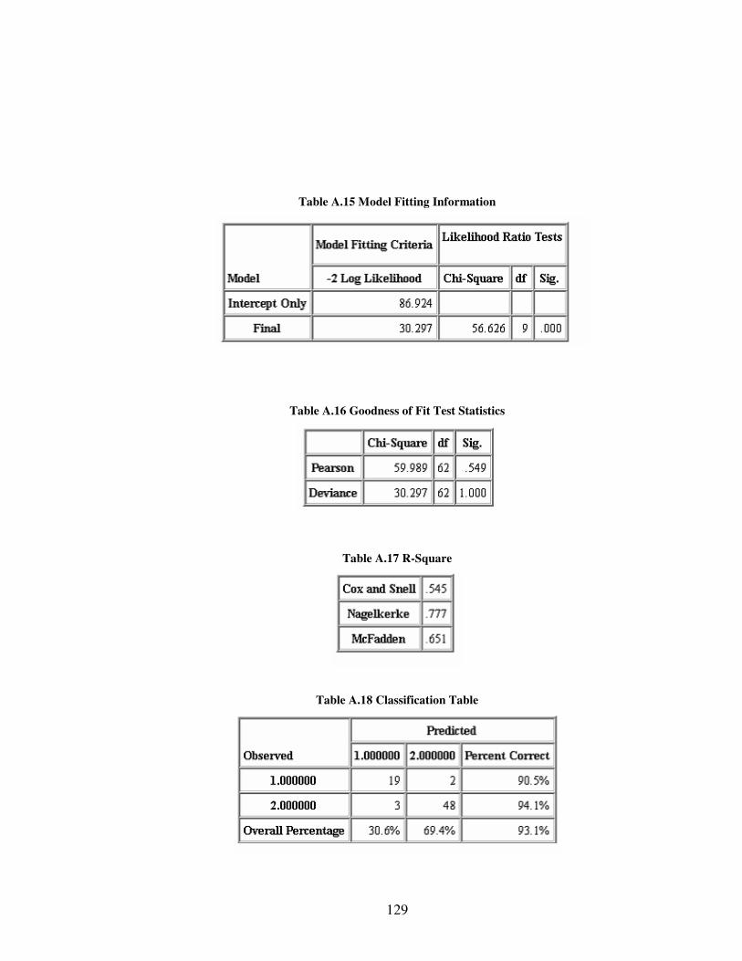
129

Table A.15 Model Fitting Information

Table A.16 Goodness of Fit Test Statistics

Table A.17 R-Square

Table A.18 Classification Table

130

2) Model 2

Table A.19 Parameter Estimates for Model 2

Table A.20 Model Fitting Information

Question 13_2=1

Question 13_2=2

Question 24

Question 33

Question 42

Question 43

Question 7

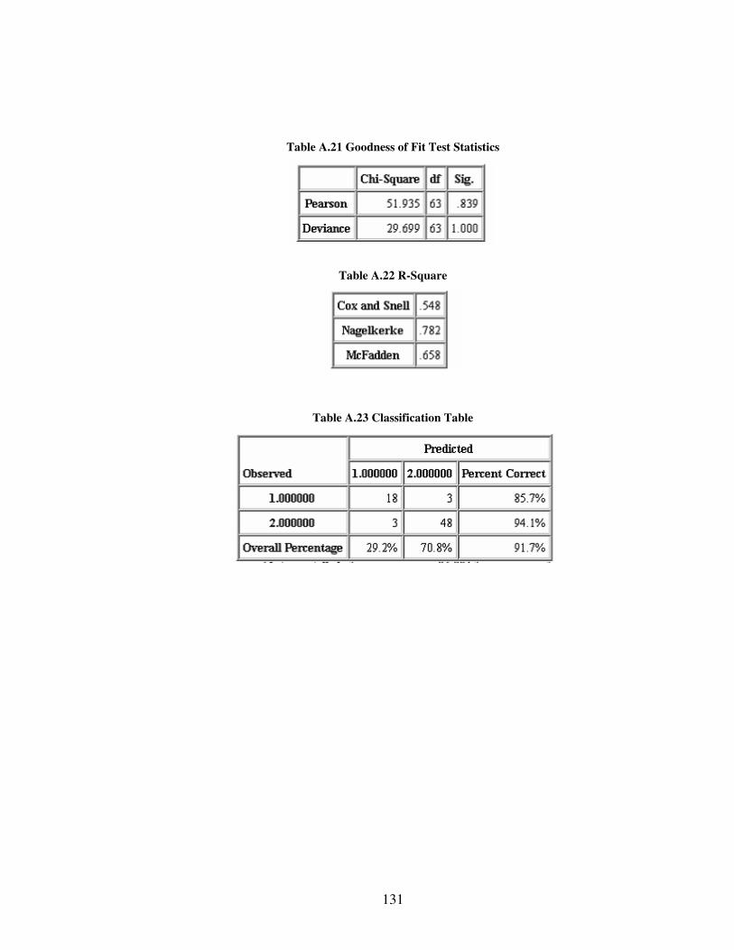
131

Table A.21 Goodness of Fit Test Statistics

Table A.22 R-Square

Table A.23 Classification Table

132

APPENDIX M

EXPLANATION OF VARIABLES IN THE MODELS

1) Model 1

X1

Question 13 has 4 choices in the questionnaire.

Question 13: How frequently do you use this vehicle?

Do not use the vehicle (0)

Through the day (1)

When necessary in a day (2)

Occasionally (on weekends and holidays) (3)

While building the model, it is seen that there is no significant difference between

choices 0, 1 and 3. However choice 2 is significantly different from them. This situation

is understood by observing the p values of each level in the model. In the previous

model, where choice 3 is the reference level for example, p values of choices 0 and 1 are

greater than 0.05, but p value of choice 2 is less then 0.05. Therefore it is decided to

create 3 dummy variables for each level (as shown below). Then the stepwise procedure

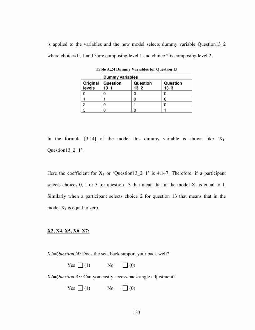
133

is applied to the variables and the new model selects dummy variable Question13_2

where choices 0, 1 and 3 are composing level 1 and choice 2 is composing level 2.

Table A.24 Dummy Variables for Question 13

Dummy variables

Original levels

Question 13_1

Question 13_2

Question 13_3

0 0 0 0

1 1 0 0

2 0 1 0

3 0 0 1

In the formula [3.14] of the model this dummy variable is shown like ‘X1:

Question13_2=1’.

Here the coefficient for X1 or ‘Question13_2=1’ is 4.147. Therefore, if a participant

selects choices 0, 1 or 3 for question 13 that mean that in the model X1 is equal to 1.

Similarly when a participant selects choice 2 for question 13 that means that in the

model X1 is equal to zero.

X2, X4, X5, X6, X7:

X2=Question24: Does the seat back support your back well?

Yes (1) No (0)

X4=Question 33: Can you easily access back angle adjustment?

Yes (1) No (0)

134

X5=Question 42: Does this arm rest meet your expectations?

Yes (1) No (0)

X6=Question 43: Is the stiffness of the seat suitable for you?

Yes (1) No (0)

X7=Question 7: Monthly income of your family?

Less than 1500 YTL (1)

Between 1500-3500 YTL (2)

Greater than 3500 YTL (3)

These questions are treated as continuous variables in the model since they show ordinal

behavior.

X3

What is your expectation from the head restraint?

Question 27: Rest my head? � (1) if it is selected, (0) if it is not selected

In the formula [3.16] of the model this variable is shown like ‘X 3: Question27=0’. Here

the coefficient for X3 or ‘Question27=0’ is 1.882. Therefore, if a participant selects the

box of question 27 then X3 is equal to zero. Similarly when a participant does not select

the box then in the model X3 is equal to 1.

135

X8 and X9

Question 76 and question 85 are about some anthropometrical measures. Question 76 is

weight and question 85 is hip-popliteal length. In the logistic regression analysis all of

the anthropometrical measures are used after standardized. Therefore X8 is the

standardized form of the weight and X9 is the standardized form of the hip-popliteal

length.

Standardization is applied by using the equation [3.6]

2) Model 2

X1:

X1 represents question 13 as explained in Appendix M.

X2, X3, X4, X5 and X6

X2, X3, X4, X5 and X6 represent questions 24, 33, 42, 43 and 7 as explained in

Appendix M.

X7 and X8

X7 is the interaction of standardized PC1 and standardized PC2, and X8 is the

interaction of standardized PC1 and standardized PC4.

As stated in Section 3.3.4 principle components are generated by using anthropometrical

measures in order to have independent variables in the model. In model 2, principle

136

components are used instead of individual anthropometrical measures. Since principle

components are continuous variables in different scales, they are used after standardized.

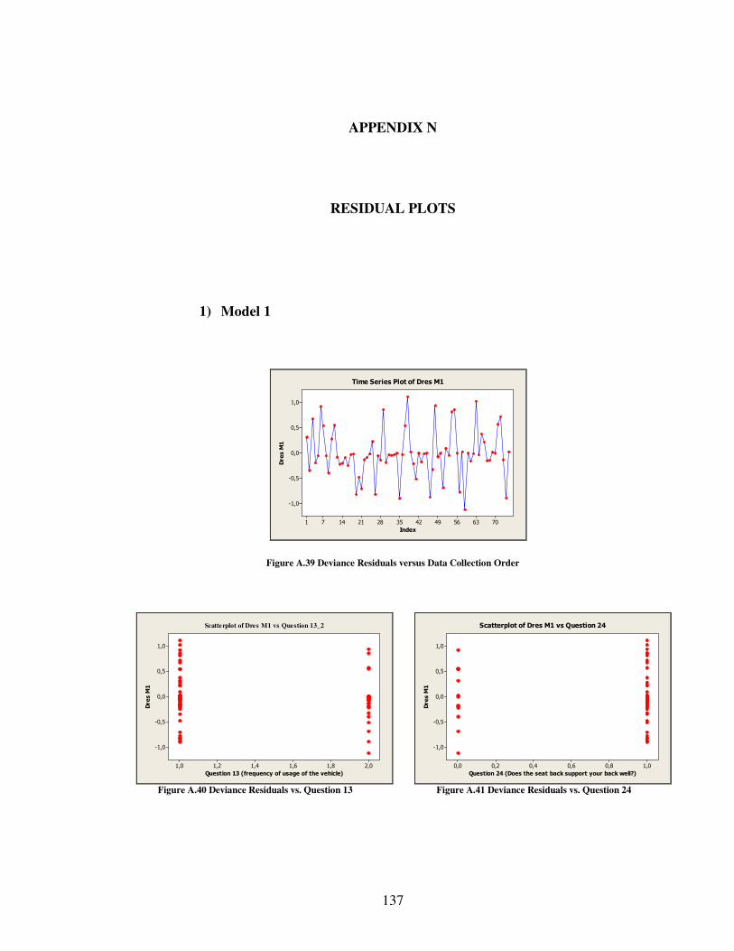
137

APPENDIX N

RESIDUAL PLOTS

1) Model 1

70635649423528211471

1,0

0,5

0,0

-0,5

-1,0

Index

Dres M1

Time Series Plot of Dres M1

Figure A.39 Deviance Residuals versus Data Collection Order

2,01,81,61,41,21,0

1,0

0,5

0,0

-0,5

-1,0

Question 13 (frequency of usage of the vehicle)

Dres M1

Scatterplot of Dres M1 vs Question 13_2

Figure A.40 Deviance Residuals vs. Question 13

1,00,80,60,40,20,0

1,0

0,5

0,0

-0,5

-1,0

Question 24 (Does the seat back support your back well?)

Dres M1

Scatterplot of Dres M1 vs Question 24

Figure A.41 Deviance Residuals vs. Question 24

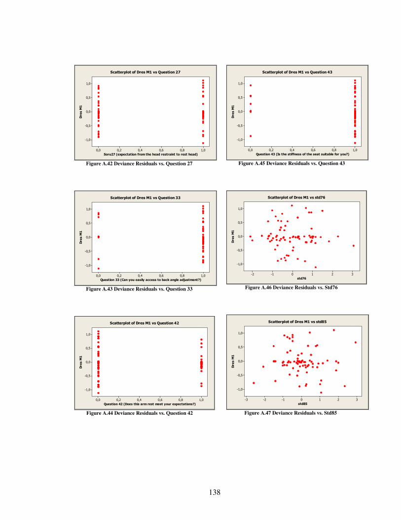
138

1,00,80,60,40,20,0

1,0

0,5

0,0

-0,5

-1,0

Soru27 (expectation from the head restraint to rest head)

Dres M1

Scatterplot of Dres M1 vs Question 27

Figure A.42 Deviance Residuals vs. Question 27

1,00,80,60,40,20,0

1,0

0,5

0,0

-0,5

-1,0

Question 33 (Can you easily access to back angle adjustment?)

Dres M1

Scatterplot of Dres M1 vs Question 33

Figure A.43 Deviance Residuals vs. Question 33

1,00,80,60,40,20,0

1,0

0,5

0,0

-0,5

-1,0

Question 42 (Does this arm rest meet your expectations?)

Dres M1

Scatterplot of Dres M1 vs Question 42

Figure A.44 Deviance Residuals vs. Question 42

1,00,80,60,40,20,0

1,0

0,5

0,0

-0,5

-1,0

Question 43 (Is the stiffness of the seat suitable for you?)

Dres M1

Scatterplot of Dres M1 vs Question 43

Figure A.45 Deviance Residuals vs. Question 43

3210-1-2

1,0

0,5

0,0

-0,5

-1,0

std76

Dres M1

Scatterplot of Dres M1 vs std76

Figure A.46 Deviance Residuals vs. Std76

3210-1-2-3

1,0

0,5

0,0

-0,5

-1,0

std85

Dres M1

Scatterplot of Dres M1 vs std85

Figure A.47 Deviance Residuals vs. Std85

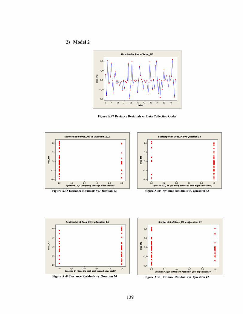
139

2) Model 2

70635649423528211471

1,0

0,5

0,0

-0,5

-1,0

Index

Dres_M2

Time Series Plot of Dres_M2

Figure A.47 Deviance Residuals vs. Data Collection Order

2,01,81,61,41,21,0

1,0

0,5

0,0

-0,5

-1,0

Question 13_2 (frequency of usage of the vehicle)

Dres_M2

Scatterplot of Dres_M2 vs Question 13_2

Figure A.48 Deviance Residuals vs. Question 13

1,00,80,60,40,20,0

1,0

0,5

0,0

-0,5

-1,0

Question 24 (Does the seat back support your back?)

Dres_M2

Scatterplot of Dres_M2 vs Question 24

Figure A.49 Deviance Residuals vs. Question 24

1,00,80,60,40,20,0

1,0

0,5

0,0

-0,5

-1,0

Question 33 (Can you easily access to back angle adjustment)

Dres_M2

Scatterplot of Dres_M2 vs Question 33

Figure A.50 Deviance Residuals vs. Question 33

1,00,80,60,40,20,0

1,0

0,5

0,0

-0,5

-1,0

Question 42 (Does this arm rest meet your expectations?)

Dres_M2

Scatterplot of Dres_M2 vs Question 42

Figure A.51 Deviance Residuals vs. Question 42

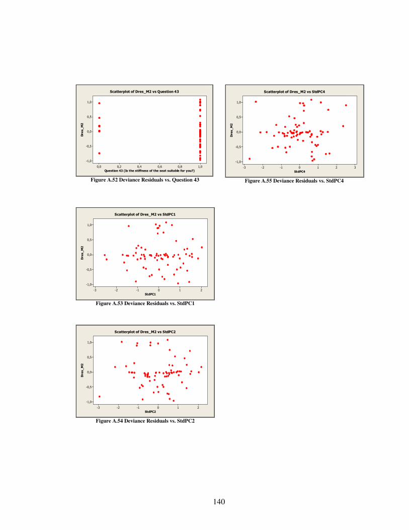
140

1,00,80,60,40,20,0

1,0

0,5

0,0

-0,5

-1,0

Question 43 (Is the stiffness of the seat suitable for you?)

Dres_M2

Scatterplot of Dres_M2 vs Question 43

Figure A.52 Deviance Residuals vs. Question 43

210-1-2-3

1,0

0,5

0,0

-0,5

-1,0

StdPC1

Dres_M2

Scatterplot of Dres_M2 vs StdPC1

Figure A.53 Deviance Residuals vs. StdPC1

210-1-2-3

1,0

0,5

0,0

-0,5

-1,0

StdPC2

Dres_M2

Scatterplot of Dres_M2 vs StdPC2

Figure A.54 Deviance Residuals vs. StdPC2

3210-1-2-3

1,0

0,5

0,0

-0,5

-1,0

StdPC4

Dres_M2

Scatterplot of Dres_M2 vs StdPC4

Figure A.55 Deviance Residuals vs. StdPC4

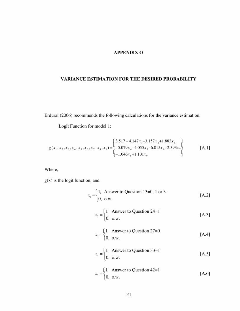
141

APPENDIX O

VARIANCE ESTIMATION FOR THE DESIRED PROBABILITY

Erdural (2006) recommends the following calculations for the variance estimation.

Logit Function for model 1:

[A.1]

Where,

g(x) is the logit function, and

1

1, Answer to Question 13=0, 1 or 3

0, o.w.x

=

[A.2]

2

1, Answer to Question 24=1

0, o.w.x

=

[A.3]

3

1, Answer to Question 27=0

0, o.w.x

=

[A.4]

4

1, Answer to Question 33=1

0, o.w.x

=

[A.5]

5

1, Answer to Question 42=1

0, o.w.x

=

[A.6]

1 2 3

1 2 3 4 5 6 7 8 9 4 5 6 7

8 9

3.517 4.147 3.157 1.882

( , , , , , , , , ) 5.079 4.055 6.015 2.393

1.046 1.101

x x x

g x x x x x x x x x x x x x

x x

+ − +

= − − − + − +

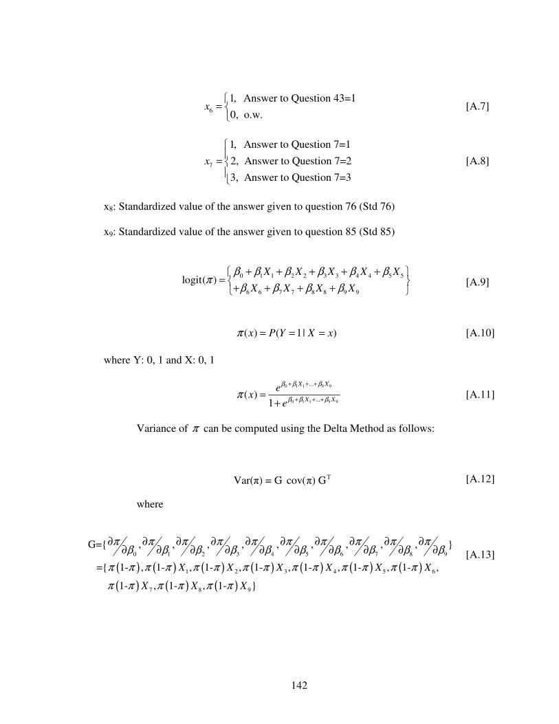
142

6

1, Answer to Question 43=1

0, o.w.x

=

[A.7]

7

1, Answer to Question 7=1

2, Answer to Question 7=2

3, Answer to Question 7=3

x

=

[A.8]

x8: Standardized value of the answer given to question 76 (Std 76)

x9: Standardized value of the answer given to question 85 (Std 85)

[A.9]

( ) ( 1| )x P Y X xπ = = = [A.10]

where Y: 0, 1 and X: 0, 1

0 1 1 9 9

0 1 1 9 9

...

...( )

1

X X

X X

ex

e

β β β

β β βπ

+ + +

+ + +=

+ [A.11]

Variance of π can be computed using the Delta Method as follows:

[A.12]

where

[A.13]

0 1 1 2 2 3 3 4 4 5 5

6 6 7 7 8 8 9 9

logit( )X X X X X

X X X X

β β β β β βπ

β β β β

+ + + + + =

+ + + +

TVar(π) = G cov(π) G

( ) ( ) ( ) ( ) ( ) ( ) ( )

( ) ( ) ( )

0 1 2 3 4 5 6 7 8 9

1 2 3 4 5 6

7 8 9

G={ , , , , , , , , , }

={ 1- , 1- , 1- , 1- , 1- , 1- , 1- ,

1- , 1- , 1- }

X X X X X X

X X X

π π π π π π π π π πβ β β β β β β β β β

π π π π π π π π π π π π π π

π π π π π π

∂ ∂ ∂ ∂ ∂ ∂ ∂ ∂ ∂ ∂∂ ∂ ∂ ∂ ∂ ∂ ∂ ∂ ∂ ∂

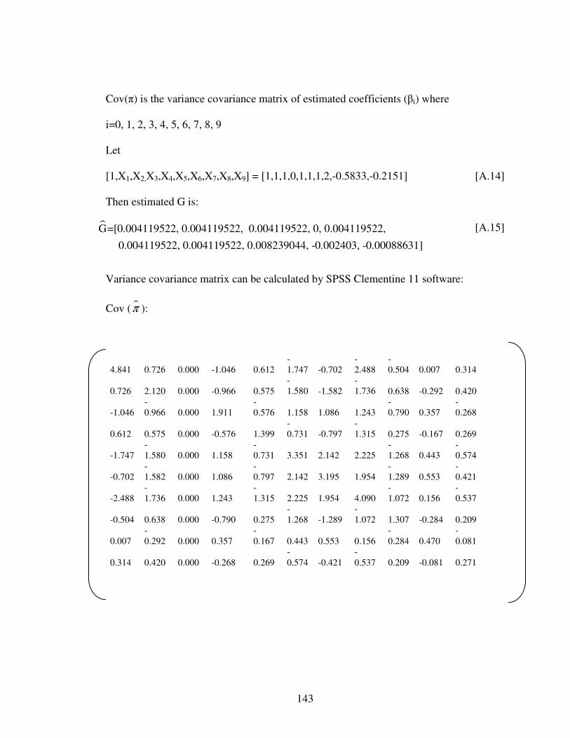
143

Cov(π) is the variance covariance matrix of estimated coefficients (βi) where

i=0, 1, 2, 3, 4, 5, 6, 7, 8, 9

Let

[1,X1,X2,X3,X4,X5,X6,X7,X8,X9] = [1,1,1,0,1,1,1,2,-0.5833,-0.2151] [A.14]

Then estimated G is:

[A.15]

Variance covariance matrix can be calculated by SPSS Clementine 11 software:

Cov ( �π ):

4.841 0.726 0.000 -1.046 0.612 -1.747 -0.702

-2.488

-0.504 0.007 0.314

0.726 2.120 0.000 -0.966 0.575 -1.580 -1.582

-1.736 0.638 -0.292 0.420

-1.046 -0.966 0.000 1.911

-0.576 1.158 1.086 1.243

-0.790 0.357

-0.268

0.612 0.575 0.000 -0.576 1.399 -0.731 -0.797

-1.315 0.275 -0.167 0.269

-1.747 -1.580 0.000 1.158

-0.731 3.351 2.142 2.225

-1.268 0.443

-0.574

-0.702 -1.582 0.000 1.086

-0.797 2.142 3.195 1.954

-1.289 0.553

-0.421

-2.488 -1.736 0.000 1.243

-1.315 2.225 1.954 4.090

-1.072 0.156

-0.537

-0.504 0.638 0.000 -0.790 0.275 -1.268 -1.289

-1.072 1.307 -0.284 0.209

0.007 -0.292 0.000 0.357

-0.167 0.443 0.553 0.156

-0.284 0.470

-0.081

0.314 0.420 0.000 -0.268 0.269 -0.574 -0.421

-0.537 0.209 -0.081 0.271

�G=[0.004119522, 0.004119522, 0.004119522, 0, 0.004119522,

0.004119522, 0.004119522, 0.008239044, -0.002403, -0.00088631]

144

[A.16]

By using formula [A.16]:

[A.17]

TVar(π) = G cov(π) G

� ɵVar(π) = 0.0000786692

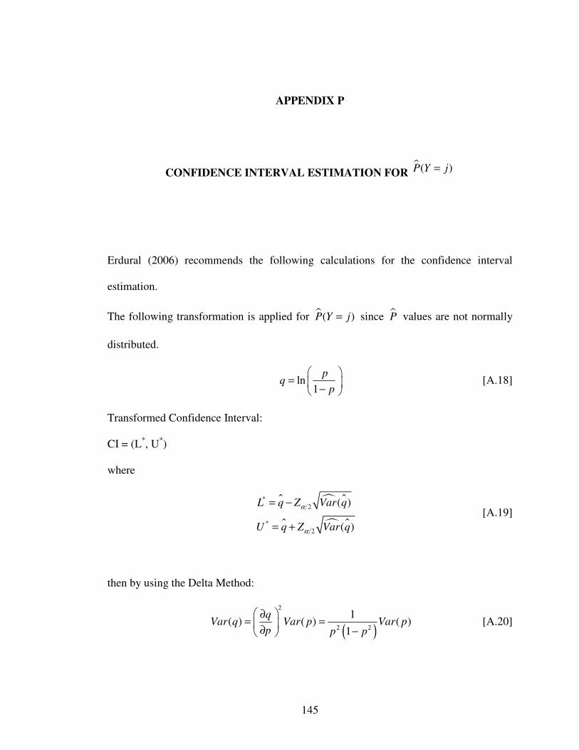
145

APPENDIX P

CONFIDENCE INTERVAL ESTIMATION FOR �( )P Y j=

Erdural (2006) recommends the following calculations for the confidence interval

estimation.

The following transformation is applied for �( )P Y j= since �P values are not normally

distributed.

ln1

pq

p

=

− [A.18]

Transformed Confidence Interval:

CI = (L*, U*)

where

ɵ � ɵ

ɵ � ɵ

*2

*2

( )

( )

L q Z Var q

U q Z Var q

α

α

= −

= +

[A.19]

then by using the Delta Method:

( )

2

2 2

1( ) ( ) ( )

1

qVar q Var p Var p

p p p

∂= =

∂ − [A.20]

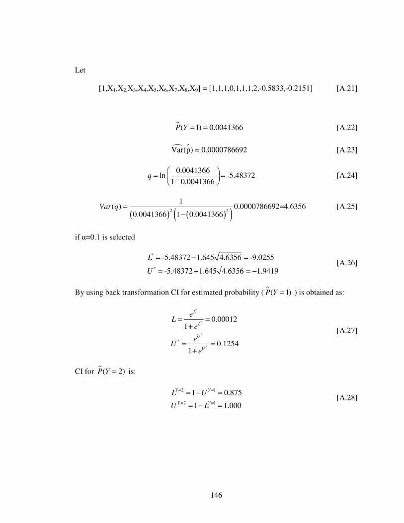
146

Let

[1,X1,X2,X3,X4,X5,X6,X7,X8,X9] = [1,1,1,0,1,1,1,2,-0.5833,-0.2151] [A.21]

�( 1) 0.0041366P Y = = [A.22]

� ɵVar(p) = 0.0000786692 [A.23]

0.0041366ln -5.48372

1 0.0041366q

= =

− [A.24]

( ) ( )( )2 2

1( ) 0.0000786692=4.6356

0.0041366 1 0.0041366Var q =

− [A.25]

if α=0.1 is selected

*

*

-5.48372 1.645 4.6356 -9.0255

-5.48372 1.645 4.6356 1.9419

L

U

= − =

= + = − [A.26]

By using back transformation CI for estimated probability ( �( 1)P Y = ) is obtained as:

*

*

*

*

*

0.000121

0.12541

L

L

U

U

eL

e

eU

e

= =+

= =+

[A.27]

CI for �( 2)P Y = is:

2 1

2 1

1 0.875

1 1.000

Y Y

Y Y

L U

U L

= =

= =

= − =

= − = [A.28]

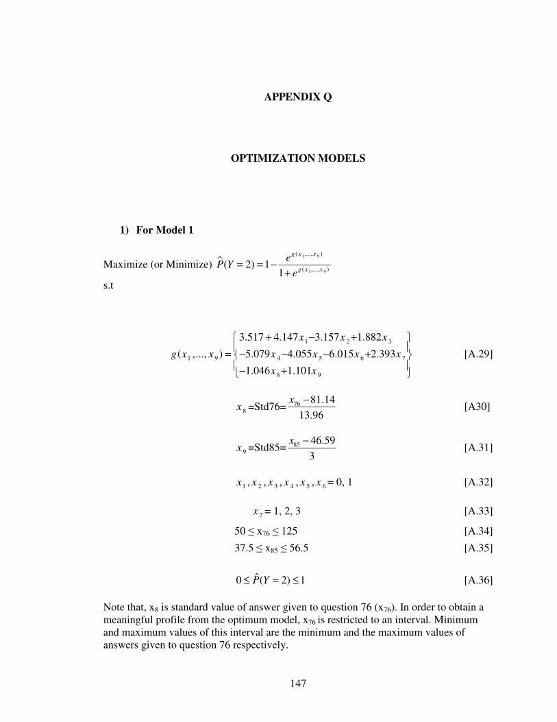
147

APPENDIX Q

OPTIMIZATION MODELS

1) For Model 1

Maximize (or Minimize) �1 9

1 9

( ,..., )

( ,..., )( 2) 1

1

g x x

g x x

eP Y

e= = −

+

s.t

1 2 3

1 9 4 5 6 7

8 9

3.517 4.147 3.157 1.882

( ,..., ) 5.079 4.055 6.015 2.393

1.046 1.101

x x x

g x x x x x x

x x

+ − +

= − − − + − +

[A.29]

8x =Std76= 76 81.14

13.96

x − [A30]

9x =Std85= 85 46.59

3

x − [A.31]

1 2 3 4 5 6, , , , ,x x x x x x = 0, 1 [A.32]

7x = 1, 2, 3 [A.33]

50 ≤ x76 ≤ 125 [A.34]

37.5 ≤ x85 ≤ 56.5 [A.35]

ˆ0 ( 2) 1P Y≤ = ≤ [A.36]

Note that, x8 is standard value of answer given to question 76 (x76). In order to obtain a meaningful profile from the optimum model, x76 is restricted to an interval. Minimum and maximum values of this interval are the minimum and the maximum values of answers given to question 76 respectively.

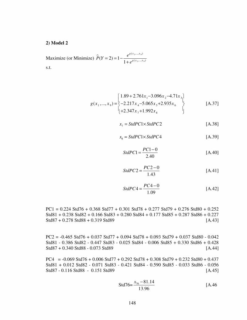
148

2) Model 2

Maximize (or Minimize) �1 9

1 9

( ,..., )

( ,..., )( 2) 1

1

g x x

g x x

eP Y

e= = −

+

s.t.

1 2 3

1 9 4 5 6

7 8

1.89 2.761 3.096 4.71

( ,..., ) 2.217 5.065 2.935

2.347 1.992

x x x

g x x x x x

x x

+ − −

= − − + + +

[A.37]

7 1 2x StdPC StdPC= × [A.38]

8 1 4x StdPC StdPC= × [A.39]

1 0

12.40

PCStdPC

−= [A.40]

2 0

21.43

PCStdPC

−= [A.41]

4 0

41.09

PCStdPC

−= [A.42]

PC1 = 0.224 Std76 + 0.368 Std77 + 0.301 Std78 + 0.277 Std79 + 0.276 Std80 + 0.252 Std81 + 0.238 Std82 + 0.166 Std83 + 0.280 Std84 + 0.177 Std85 + 0.287 Std86 + 0.227 Std87 + 0.278 Std88 + 0.319 Std89 [A.43] PC2 = -0.465 Std76 + 0.037 Std77 + 0.094 Std78 + 0.093 Std79 + 0.037 Std80 - 0.042 Std81 - 0.386 Std82 - 0.447 Std83 - 0.025 Std84 - 0.006 Std85 + 0.330 Std86 + 0.428 Std87 + 0.340 Std88 - 0.073 Std89 [A.44] PC4 = -0.069 Std76 + 0.006 Std77 + 0.292 Std78 + 0.308 Std79 + 0.232 Std80 + 0.437 Std81 + 0.012 Std82 - 0.071 Std83 - 0.421 Std84 - 0.590 Std85 - 0.033 Std86 - 0.056 Std87 - 0.116 Std88 - 0.151 Std89 [A.45]

Std76= 76 81.14

13.96

x − [A.46

149

Std77= 77 173.81

6.63

x − [A.47]

Std78= 78 74.10

4.27

x − [A.48]

Std79= 79 45.72

2.46

x − [A.49]

Std80= 80 34.21

2.97

x − [A.50]

Std81= 81 18.84

0.96

x − [A.51]

Std82= 82 46.46

3.29

x − [A.52]

Std83= 83 40.39

2.96

x − [A.53]

Std84= 84 56.61

3.17

x − [A.54]

Std85= 85 46.59

3.22

x − [A.55]

Std86= 86 87.49

4.20

x − [A.56]

Std87= 87 75.18

4.40

x − [A.57]

Std88= 88 59.17

3.43

x − [A.58]

Std89= 89 55.49

2.79

x − [A.59]

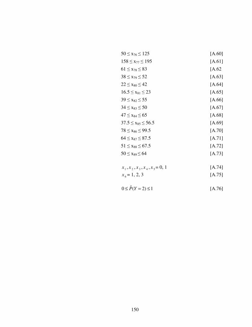
150

50 ≤ x76 ≤ 125 [A.60]

158 ≤ x77 ≤ 195 [A.61]

61 ≤ x78 ≤ 83 [A.62

38 ≤ x79 ≤ 52 [A.63]

22 ≤ x80 ≤ 42 [A.64]

16.5 ≤ x81 ≤ 23 [A.65]

39 ≤ x82 ≤ 55 [A.66]

34 ≤ x83 ≤ 50 [A.67]

47 ≤ x84 ≤ 65 [A.68]

37.5 ≤ x85 ≤ 56.5 [A.69]

78 ≤ x86 ≤ 99.5 [A.70]

64 ≤ x87 ≤ 87.5 [A.71]

51 ≤ x88 ≤ 67.5 [A.72]

50 ≤ x89 ≤ 64 [A.73]

1 2 3 4 5, , , ,x x x x x = 0, 1 [A.74]

6x = 1, 2, 3 [A.75]

ˆ0 ( 2) 1P Y≤ = ≤ [A.76]

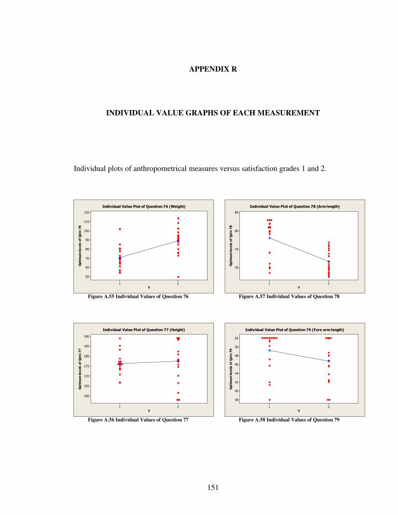
151

APPENDIX R

INDIVIDUAL VALUE GRAPHS OF EACH MEASUREMENT

Individual plots of anthropometrical measures versus satisfaction grades 1 and 2.

21

120

110

100

90

80

70

60

50

Y

Optimum levels of Qstn 76

Individual Value Plot of Question 76 (Weight)

Figure A.55 Individual Values of Question 76

21

190

185

180

175

170

165

160

Y

Optimum levels of Qstn 77

Individual Value Plot of Question 77 (Height)

Figure A.56 Individual Values of Question 77

21

85

80

75

70

Y

Optimum levels of Qstn 78

Individual Value Plot of Question 78 (Arm length)

Figure A.57 Individual Values of Question 78

21

52

50

48

46

44

42

40

38

Y

Optimum levels of Qstn 79

Individual Value Plot of Question 79 (Fore arm length)

Figure A.58 Individual Values of Question 79

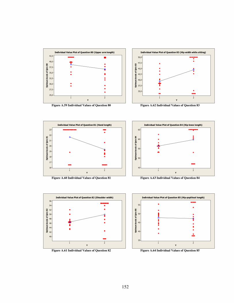
152

21

42,5

40,0

37,5

35,0

32,5

30,0

27,5

25,0

Y

Optimum levels of Qstn 80

Individual Value Plot of Question 80 (Upper arm length)

Figure A.59 Individual Values of Question 80

21

23

22

21

20

19

18

17

16

Y

Optimum levels of Qstn 81

Individual Value Plot of Question 81 (Hand length)

Figure A.60 Individual Values of Question 81

21

56

54

52

50

48

46

44

42

40

Y

Optimum levels of Qstn 82

Individual Value Plot of Question 82 (Shoulder width)

Figure A.61 Individual Values of Question 82

21

50,0

47,5

45,0

42,5

40,0

37,5

35,0

Y

Optimum levels of Qstn 83

Individual Value Plot of Question 83 (Hip width while sitting)

Figure A.62 Individual Values of Question 83

21

65

60

55

50

45

Y

Optimum levels of Qstn 84

Individual Value Plot of Question 84 (Hip-knee length)

Figure A.63 Individual Values of Question 84

21

55

50

45

40

35

Y

Optimum levels of Qstn 85

Individual Value Plot of Question 85 (Hip-popliteal length)

Figure A.64 Individual Values of Question 85

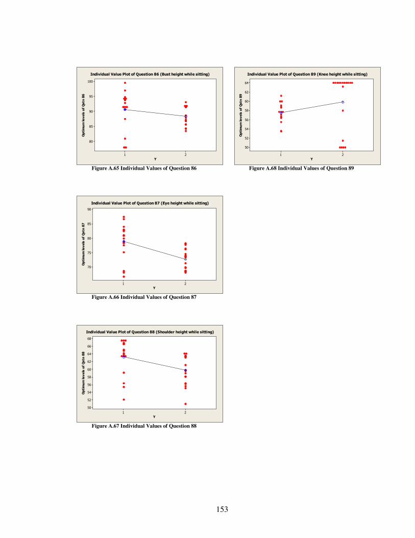
153

21

100

95

90

85

80

Y

Optimum levels of Qstn 86

Individual Value Plot of Question 86 (Bust height while sitting)

Figure A.65 Individual Values of Question 86

21

90

85

80

75

70

Y

Optimum levels of Qstn 87

Individual Value Plot of Question 87 (Eye height while sitting)

Figure A.66 Individual Values of Question 87

21

68

66

64

62

60

58

56

54

52

50

Y

Optimum levels of Qstn 88

Individual Value Plot of Question 88 (Shoulder height while sitting)

Figure A.67 Individual Values of Question 88

21

64

62

60

58

56

54

52

50

Y

Optimum levels of Qstn 89

Individual Value Plot of Question 89 (Knee height while sitting)

Figure A.68 Individual Values of Question 89