Embed Size (px)
Citation preview

Modeling and Analysis of Electric Vehicle Charging Interface
T. P. EZHIL REENA JOY

TH-1345_TPERJOY

Modeling and Analysis of Electric Vehicle Charging
Interface
A
Thesis Submitted
in Partial Fulfilment of the Requirements
for the Degree of
DOCTOR OF PHILOSOPHY
By
T. P. EZHIL REENA JOY
Department of Electronics and Electrical Engineering
Indian Institute of Technology Guwahati
Guwahati - 781 039, INDIA.
March, 2015
TH-1345_TPERJOY

TH-1345_TPERJOY

Certificate
This is to certify that the thesis entitled “Modeling and Analysis of Electric Vehicle Charg-
ing Interface”, submitted by T. P. Ezhil Reena Joy (09610209), a research scholar in the De-
partment of Electronics & Electrical Engineering, Indian Institute of Technology Guwahati, for the
award of the degree of Doctor of Philosophy, has been carried out by her under my supervision
and guidance. The thesis has fulfilled all requirements as per the regulations of the Institute and in
my opinion has reached the standard needed for submission. The results embodied in this thesis have
not been submitted to any other University or Institute for the award of any degree or diploma.
Dated: Dr. Praveen Kumar
Guwahati. Dept. of Electronics & Electrical Engg.
Indian Institute of Technology Guwahati
Guwahati - 781039, Assam, India.
TH-1345_TPERJOY

TH-1345_TPERJOY

To my mother
with love and gratitude ...
TH-1345_TPERJOY

TH-1345_TPERJOY

Acknowledgements
First and foremost, I thank my Lord and Savior Jesus Christ for granting me grace, time, health
and essential wisdom to complete my research work. If words can express my thoughts and love then,
with all my heart and with all my love I express my thanks to my loving mother L. Puspha Joy
for her kindness, love, encouragement and prayers throughout my research. I am highly thankful to
Prof. Somnath Majhi and his committee members for selecting me in interview and have given a
chance to pursue doctoral research in this Institute. It is my bounden duty to thank Government of
India, for establishing IIT Guwahati and for providing all facilities, web resources and scholarship to
do the research. Then I knot my arms and express my sincere gratitude to my thesis supervisor Dr.
Praveen Kumar, for the support and guidance given for me throughout my research work. I found
my supervisor has some uniqueness in his guidance. I thank my supervisor, for guiding me to choose
all my courses in my first year. I am grateful that he has helped me to complete all my academic
requirements on time throughout my research period. I acknowledge that he has spent enough time in
discussing my research problems, teaching me related basics and used to work my simulations during
my initial days in Phd. In my second and third year, he taught me the importance to ‘think’ of a
particular problem. He has also trained me how to structure the ideas in form of article. I acknowledge
him gratefully that all chapters in this thesis are his ideas and that was worked out and elaborated
in each pages. He has also spent his time to coordinate each work and get it done with a team by
monitoring it continuously. I believe over the past years, I have absorbed some of his tactics in doing
research. Under his guidance, I got acquainted with many software tools and learned many technical
issues especially about electric vehicles, charging system, contactless system, energy storage systems
and about other distributed energy resource. Along with my supervisor, I would like to thank Prof.
Sanjay Kumar Bose, Prof. Pradeep Gururaj Yammiyavar and Prof. Somanath Majhi for serving in
my doctoral exam committee. My doctoral committee members are always on time and spend their
precious time to evaluate the progress of my work. Their suggestions are valuable and they have asked
questions, which helped me to widen my knowledge and research work.
I am also indebted to my post graduate mentors especially Professor Anug Jaiprakash Kellogg and
Dr. F.T. Josh at Karunya University, who have taught most of my courses in Power Electronics and
made me to reach this stage. I must thank my Master program thesis supervisor Dr. T. Aruldoss
TH-1345_TPERJOY

Albert Victorie, he is my first inspiration and one of the reasoner that i pursue my doctoral research.
I also thank all my undergraduate mentors including Dr. N. Carolin Mabel and Mr. N.M. Spencer
Prathap Singh for teaching me various courses in Engineering. Further, I am grateful to my school
teachers who by delivering liberal yet rigorous education and prepared me to reach this level. My
special thanks to Sister Lucia, Felix miss and Fathima miss, they are unforgettable and played a good
role in my education. My teachers not only taught science and maths but also they have been a role
model for humanity, kindness and dedication in work. In addition, I must thank my former colleague
Ramesh and Aneesa, they are the prime reason for me to join in this Institute. I thank my colleagues
here, Mukesh Singh, Kannan, Ankit, Brijesh and Guatam for their research collaboration. I could
always discuss with them and it gave a concrete support in my research. My special thanks to Kannan
and Ankit, they have always helped me whenever I approached them. I must thank Ambika mam
and Josephine mams’ family for helping me to grow spiritually. It has helped me to overcome my
depression and my short temper. They are so kind enough and always greeted everyone and served
delicious food. My special thanks to Ambika mam for taking care during my sick days. I thank my
friends specially Sonali, Resmi, Sheeba, Malathi and Usha, I really had a good time with them. My
special thanks to Usha and her help during my last days of my Phd. She kept an eye on me and
insisted me to finish all my works quickly. I am grateful to all my other friends in IITG, my juniors
and beyond, who have kept me happy and made me cheerful. I also acknowledge all the support and
encouragements provided to me by other Professors and department non-teaching staffs and friends
throughout my work. I also thank all the Professors who spend time to review my article. I pray to
God to help all those who helped me. May God shower their lives with blessings according to Ezekiel
34:26.
Last but not the least, I thank all the readers who read my thesis. The chapters of this thesis
are carefully done and I hope all the readers would surely gain knowledge on electric vehicle charging
system and contactless system. Many relevant references are cited at the last pages of the thesis,
which will also help you to understand and learn more about the recent technologies in EV charging
systems. I thank one and all. Thank you
Thank you
(Reena Prathaf)
x
TH-1345_TPERJOY

Abstract
As the energy demand and environmental issues are becoming increasingly prominent, the future
of transportation is believed to be based on electric vehicles (EV). Apparently, the research on EV
charging systems are very important for the development and popularization of EVs. This thesis
describes the design, control and analysis of both contact based and contactless power transfer system
suitable for EV charging system applications. The first chapter describes the classification of EV
charging systems and has given the overview of contactless charging system including the principle of
bidirectional charging system. The chapter has summarized the major challenges and goals identified
in this research. The second chapter of this thesis has investigated the deployment of EVs aggregation
through contact based charging system for the provision of voltage regulation at the distribution node.
This chapter has modeled a contact based charging station and its control to coordinate multiple EVs
arrived in the charging station. For this purpose, a charging station is modeled with multiple charging
systems using ac-dc converter and a series connected dc-dc converter with suitable controllers to
facilitate EVs of different ratings to charge and discharge. The developed charging system has been
operated bidirectional to transfer power on both forward and reverse direction. This bidirectional
power flow functionality of the charging system has been referred as grid-to-vehicle and vehicle-to-
grid technology. The validation of the study is carried out for a 300kW charging station having 35
charging systems connected with EVs of different battery ratings. This charging system has been
modeled to handle high power (up to a hundred kW) and high energy capacity (up to tens of kWh)
batteries. However, charging and discharging such high capacity batteries using contact based charging
systems in real time may cause the dangerous possibility of high voltage contact. If EVs are charged
using contact-less technique, there are clear advantages to be gained in terms of safety, reliability
and endurance. The third chapter of this thesis has focused on modeling, design and control aspects
of parallel connected multiple contactless charging system connected to a common ac bus network.
xi
TH-1345_TPERJOY

Two types of charging station architectures are discussed. An electric equivalent circuit model has
been used to describe the steady state electrical characteristics of contactless coil. The model has
been validated with 500kVA charging station connected with ten 50kW charging systems. While,
the contactless coil in the charging systems are designed using a fixed coupling factor assuming a
perfect alignment between the coils. However, the usage of contactless system in EV battery charging
applications are usually misaligned due to uneven road surface, tyre pressure, passenger weight etc.
Therefore, the design of complete charging system becomes more complex due to this variations in
the magnetic coupling between the coils. The variations in magnetic coupling affects the mutual
inductance (MI) value and thereby causes fluctuations in the output voltage and affects the stability
of the system. Therefore, an analytical approach is presented in the fourth chapter of the thesis
to compute MI value with all its lateral and angular misalignments. The primary coil geometry is
modelled as a straight line conductors and the MI value is calculated using flux linked to the secondary
coil due to the primary coil. The method works by approximating the area of secondary coil and the
flux distribution is calculated using Biot-Savart law. The results of computed MI value by analytical
method are validated by finite element analysis and an experimental set-up. The values computed by
three methods in all cases are in good agreement. Further, it has been observed, due to large leakage
inductance and reduced magnetizing inductance, the value of MI gradually decreases when the distance
increases. Therefore, compensation capacitors are required at the primary and secondary side of the
contactless coil to reduce VA rating of the power supply and to increase the power transfer capability.
The fifth chapter of this thesis presents an experimental study of four compensation topologies. Electric
equivalent circuit model along with compensation topologies are developed to explain the mechanism
of power transfer. The study investigates the behavior of contactless system and its characteristics
plots are generated for wide range of frequency, load and distance such that the real time situations of
contactless systems can be analyzed. The final analysis compares the efficiency of four compensation
topology and its results are reported. The sixth chapter of the thesis has summarized the conclusion
of the complete research work with some future direction of work.
xii
TH-1345_TPERJOY

Contents
List of Figures xix
List of Tables xxv
List of Acronyms xxvii
List of Symbols xxxi
List of Publications xxxv
1 Introduction 1
1.1 Overview . . . . . . . . . . . . . . . . . . . . . . . . . . . . . . . . . . . . . . . . . . . 3
1.2 Electric vehicles and charging systems . . . . . . . . . . . . . . . . . . . . . . . . . . . 4
1.2.1 Classification based on the location . . . . . . . . . . . . . . . . . . . . . . . . . 4
1.2.2 Classification based on the charging level . . . . . . . . . . . . . . . . . . . . . 6
1.2.3 Classification based on the charging scheme . . . . . . . . . . . . . . . . . . . . 6
1.2.4 Classification based on the charging method . . . . . . . . . . . . . . . . . . . . 8
1.3 Contactless system . . . . . . . . . . . . . . . . . . . . . . . . . . . . . . . . . . . . . . 8
1.3.1 Theory of CPT system . . . . . . . . . . . . . . . . . . . . . . . . . . . . . . . . 9
1.3.1.1 Mutual flux and mutual inductance . . . . . . . . . . . . . . . . . . . 9
1.3.1.2 Leakage flux . . . . . . . . . . . . . . . . . . . . . . . . . . . . . . . . 11
1.3.1.3 Contactless coils . . . . . . . . . . . . . . . . . . . . . . . . . . . . . . 12
1.4 Contactless charging and electric vehicles . . . . . . . . . . . . . . . . . . . . . . . . . 15
1.4.1 Bidirectional charging systems . . . . . . . . . . . . . . . . . . . . . . . . . . . 16
1.4.2 Vehicle-to-grid (V2G) and Grid-to-vehicle (G2V) technology . . . . . . . . . . 17
1.5 Major challenges and identified goals . . . . . . . . . . . . . . . . . . . . . . . . . . . . 18
1.6 Contributions of this thesis . . . . . . . . . . . . . . . . . . . . . . . . . . . . . . . . . 20
1.7 Thesis organization . . . . . . . . . . . . . . . . . . . . . . . . . . . . . . . . . . . . . . 22
xiii
TH-1345_TPERJOY

Contents
2 Modeling of Contact based Charging Station for Voltage Regulation 23
2.1 Introduction . . . . . . . . . . . . . . . . . . . . . . . . . . . . . . . . . . . . . . . . . . 25
2.2 Voltage regulation at distribution node . . . . . . . . . . . . . . . . . . . . . . . . . . . 28
2.2.1 Regulatory requirements . . . . . . . . . . . . . . . . . . . . . . . . . . . . . . . 28
2.2.2 Distribution node voltage control . . . . . . . . . . . . . . . . . . . . . . . . . . 28
2.3 Frame work of simulation model . . . . . . . . . . . . . . . . . . . . . . . . . . . . . . 29
2.3.1 Distribution system . . . . . . . . . . . . . . . . . . . . . . . . . . . . . . . . . 29
2.3.2 Layout of charging station (CS) . . . . . . . . . . . . . . . . . . . . . . . . . . . 30
2.3.3 Battery system . . . . . . . . . . . . . . . . . . . . . . . . . . . . . . . . . . . . 31
2.4 Problem definition . . . . . . . . . . . . . . . . . . . . . . . . . . . . . . . . . . . . . . 32
2.4.1 Fuzzy logic control (FLC) . . . . . . . . . . . . . . . . . . . . . . . . . . . . . . 33
2.4.2 Aggregator . . . . . . . . . . . . . . . . . . . . . . . . . . . . . . . . . . . . . . 35
2.4.3 Charging system . . . . . . . . . . . . . . . . . . . . . . . . . . . . . . . . . . . 36
2.4.3.1 CC-CV control . . . . . . . . . . . . . . . . . . . . . . . . . . . . . . . 36
2.4.3.2 Enhanced PLL based PWM control . . . . . . . . . . . . . . . . . . . 37
2.4.4 Control methodology . . . . . . . . . . . . . . . . . . . . . . . . . . . . . . . . . 40
2.5 Result analysis . . . . . . . . . . . . . . . . . . . . . . . . . . . . . . . . . . . . . . . . 42
2.6 Conclusions . . . . . . . . . . . . . . . . . . . . . . . . . . . . . . . . . . . . . . . . . . 48
3 Theoretical Modeling of Contactless Charging Station 51
3.1 Introduction . . . . . . . . . . . . . . . . . . . . . . . . . . . . . . . . . . . . . . . . . . 53
3.2 Modeling of contactless charging station . . . . . . . . . . . . . . . . . . . . . . . . . . 56
3.2.1 Types of charging station . . . . . . . . . . . . . . . . . . . . . . . . . . . . . . 56
3.2.2 AC bus distributed EV charging station . . . . . . . . . . . . . . . . . . . . . . 56
3.3 Bidirectional contactless charging system . . . . . . . . . . . . . . . . . . . . . . . . . 59
3.3.1 BCPT system configuration . . . . . . . . . . . . . . . . . . . . . . . . . . . . . 59
3.3.2 Contactless system modeling . . . . . . . . . . . . . . . . . . . . . . . . . . . . 59
3.4 Problem description . . . . . . . . . . . . . . . . . . . . . . . . . . . . . . . . . . . . . 62
3.4.1 Charging station control strategy . . . . . . . . . . . . . . . . . . . . . . . . . . 63
3.4.2 Scheduling algorithm . . . . . . . . . . . . . . . . . . . . . . . . . . . . . . . . . 63
3.4.3 Charging (BCPT) system . . . . . . . . . . . . . . . . . . . . . . . . . . . . . . 65
xiv
TH-1345_TPERJOY

Contents
3.4.3.1 G2V operation . . . . . . . . . . . . . . . . . . . . . . . . . . . . . . . 65
3.4.3.2 V2G operation . . . . . . . . . . . . . . . . . . . . . . . . . . . . . . . 68
3.4.4 Design of critical parameters . . . . . . . . . . . . . . . . . . . . . . . . . . . . 69
3.4.4.1 Filter circuit . . . . . . . . . . . . . . . . . . . . . . . . . . . . . . . . 69
3.4.4.2 Dc link capacitor . . . . . . . . . . . . . . . . . . . . . . . . . . . . . . 70
3.5 Simulation results . . . . . . . . . . . . . . . . . . . . . . . . . . . . . . . . . . . . . . 70
3.6 Conclusions . . . . . . . . . . . . . . . . . . . . . . . . . . . . . . . . . . . . . . . . . . 74
4 Computation of Mutual Inductance for Contactless System 77
4.1 Introduction . . . . . . . . . . . . . . . . . . . . . . . . . . . . . . . . . . . . . . . . . . 79
4.2 Possible variations of square coils . . . . . . . . . . . . . . . . . . . . . . . . . . . . . . 81
4.3 Analytical modeling of square coil . . . . . . . . . . . . . . . . . . . . . . . . . . . . . 83
4.3.1 Modeling of mutual inductance . . . . . . . . . . . . . . . . . . . . . . . . . . . 83
4.3.2 Numerical evaluation . . . . . . . . . . . . . . . . . . . . . . . . . . . . . . . . . 85
4.4 Finite element modeling of square coil . . . . . . . . . . . . . . . . . . . . . . . . . . . 86
4.5 Experimental verification . . . . . . . . . . . . . . . . . . . . . . . . . . . . . . . . . . 88
4.5.1 Description of power circuit and control circuit . . . . . . . . . . . . . . . . . . 89
4.5.2 Experimental details . . . . . . . . . . . . . . . . . . . . . . . . . . . . . . . . . 90
4.6 Numerical results and discussion . . . . . . . . . . . . . . . . . . . . . . . . . . . . . . 92
4.6.1 Perfect alignment - vertical and planar variation . . . . . . . . . . . . . . . . . 93
4.6.2 Lateral misalignment - horizontal and planar variation . . . . . . . . . . . . . . 95
4.6.3 Angular misalignment . . . . . . . . . . . . . . . . . . . . . . . . . . . . . . . . 96
4.6.4 Both lateral and angular misalignment . . . . . . . . . . . . . . . . . . . . . . . 97
4.7 Conclusions . . . . . . . . . . . . . . . . . . . . . . . . . . . . . . . . . . . . . . . . . . 99
5 Compensation Topologies for Contactless System 101
5.1 Introduction . . . . . . . . . . . . . . . . . . . . . . . . . . . . . . . . . . . . . . . . . . 103
5.2 Steady state electric circuit analysis . . . . . . . . . . . . . . . . . . . . . . . . . . . . 106
5.2.1 Compensation topologies . . . . . . . . . . . . . . . . . . . . . . . . . . . . . . 106
5.2.2 Mutual inductance coupling model . . . . . . . . . . . . . . . . . . . . . . . . . 107
5.2.3 Series-series (SS) compensation topology . . . . . . . . . . . . . . . . . . . . . . 108
5.2.4 Series-parallel (SP) compensation topology . . . . . . . . . . . . . . . . . . . . 111
xv
TH-1345_TPERJOY

Contents
5.2.5 Parallel-series (PS) compensation topology . . . . . . . . . . . . . . . . . . . . 113
5.2.6 Parallel-parallel (PP) compensation topology . . . . . . . . . . . . . . . . . . . 115
5.3 Description of experimental set-up . . . . . . . . . . . . . . . . . . . . . . . . . . . . . 117
5.3.1 Design stages . . . . . . . . . . . . . . . . . . . . . . . . . . . . . . . . . . . . . 117
5.3.2 Block diagram . . . . . . . . . . . . . . . . . . . . . . . . . . . . . . . . . . . . 118
5.3.3 Power circuit and coil description . . . . . . . . . . . . . . . . . . . . . . . . . . 119
5.3.4 Control circuit description . . . . . . . . . . . . . . . . . . . . . . . . . . . . . . 121
5.4 Results and discussion . . . . . . . . . . . . . . . . . . . . . . . . . . . . . . . . . . . . 124
5.5 Conclusions . . . . . . . . . . . . . . . . . . . . . . . . . . . . . . . . . . . . . . . . . . 137
6 Conclusions and Future Work 139
6.1 Concluding remarks . . . . . . . . . . . . . . . . . . . . . . . . . . . . . . . . . . . . . 141
6.1.1 Introduction chapter . . . . . . . . . . . . . . . . . . . . . . . . . . . . . . . . . 141
6.1.2 Modeling of Contact based Charging Station for Voltage Regulation . . . . . . 141
6.1.3 Theoretical Modeling of Contactless Charging Station . . . . . . . . . . . . . . 142
6.1.4 Computation of Mutual Inductance for Contactless System . . . . . . . . . . . 142
6.1.5 Compensation Topologies for Contactless System . . . . . . . . . . . . . . . . . 143
6.2 Suggestions for future work . . . . . . . . . . . . . . . . . . . . . . . . . . . . . . . . . 144
6.2.1 Future research on reducing the bulk semiconverters on either side of contactless
system . . . . . . . . . . . . . . . . . . . . . . . . . . . . . . . . . . . . . . . . . 144
6.2.2 Future research on wide air gap distance and misalignments in the coils . . . . 145
6.2.3 Future research on contactless coil arranged in a platform surface . . . . . . . . 145
6.2.4 Future research on bidirectional charging system . . . . . . . . . . . . . . . . . 146
6.2.5 Future research on stability studies . . . . . . . . . . . . . . . . . . . . . . . . . 146
6.2.6 Future research to calculate power losses in contact based and contactless charg-
ing system . . . . . . . . . . . . . . . . . . . . . . . . . . . . . . . . . . . . . . . 146
6.2.7 Future research on active and reactive power exchange between the grid and the
charging system . . . . . . . . . . . . . . . . . . . . . . . . . . . . . . . . . . . 146
6.2.8 Overall future research . . . . . . . . . . . . . . . . . . . . . . . . . . . . . . . . 146
A Supplementary Materials 147
A.1 Additional figures from Chapter 2 . . . . . . . . . . . . . . . . . . . . . . . . . . . . . 149
xvi
TH-1345_TPERJOY

Contents
A.2 Fuzzification & defuzzification for master control of Chapter 2 . . . . . . . . . . . . . . 150
A.3 Membership function and rule base of CC-FLC, M-FLC and PA-FLC of Chapter 2 . . 152
A.4 Fuzzification and defuzzification process for power angle control of Chapter 3 . . . . . 154
A.5 Sample calculation for mutual inductance of Chapter 4 . . . . . . . . . . . . . . . . . . 157
A.6 Remaining results of Chapter 5 . . . . . . . . . . . . . . . . . . . . . . . . . . . . . . . 157
Bibliography 163
xvii
TH-1345_TPERJOY

Contents
xviii
TH-1345_TPERJOY

List of Figures
1.1 Classification of EV chargers [1–9]. . . . . . . . . . . . . . . . . . . . . . . . . . . . . . 5
1.2 Two magnetically coupled coil. . . . . . . . . . . . . . . . . . . . . . . . . . . . . . . . 10
1.3 Representation of contactless coil as series RLC circuit. . . . . . . . . . . . . . . . . . 13
1.4 Vector diagram of series resonant circuit (a) Phasor diagram (b) Impedance diagram. 13
1.5 Block diagram of charging system . . . . . . . . . . . . . . . . . . . . . . . . . . . . . . 15
1.6 Block diagram of contactless charging system . . . . . . . . . . . . . . . . . . . . . . . 16
1.7 Bidirectional contactless charging system . . . . . . . . . . . . . . . . . . . . . . . . . 17
2.1 Illustration of CS connected at the DN. . . . . . . . . . . . . . . . . . . . . . . . . . . 28
2.2 Layout of charging station. . . . . . . . . . . . . . . . . . . . . . . . . . . . . . . . . . 30
2.3 Circuit topology of charging system. . . . . . . . . . . . . . . . . . . . . . . . . . . . . 31
2.4 Battery equivalent circuit. . . . . . . . . . . . . . . . . . . . . . . . . . . . . . . . . . . 31
2.5 Membership functions for FLC (a) node voltage (V1) (b) total energy availabilities of
EVs (Et) and (c) output power (S′). . . . . . . . . . . . . . . . . . . . . . . . . . . . . 34
2.6 Constant-current and constant-voltage charging strategy. . . . . . . . . . . . . . . . . . 37
2.7 Enhanced PLL based PWM control. . . . . . . . . . . . . . . . . . . . . . . . . . . . . 38
2.8 Power angle control (PA-FLC). . . . . . . . . . . . . . . . . . . . . . . . . . . . . . . . 39
2.9 Magnitude control (M-FLC). . . . . . . . . . . . . . . . . . . . . . . . . . . . . . . . . 39
2.10 Control process involved in EVs batteries. . . . . . . . . . . . . . . . . . . . . . . . . . 40
2.11 Control operation of single unit of charging system. . . . . . . . . . . . . . . . . . . . . 41
2.12 Comparison of node voltage using P, Q and PQ control (G2V). . . . . . . . . . . . . . 43
2.13 Comparison of node voltage using P, Q and PQ control (V2G). . . . . . . . . . . . . . 44
2.14 Comparison of node voltage using P, Q and PQ control (both G2V and V2G). . . . . 44
2.15 DC link voltage (across Cdc1). . . . . . . . . . . . . . . . . . . . . . . . . . . . . . . . . 45
xix
TH-1345_TPERJOY

List of Figures
2.16 Power factor of the charging system. . . . . . . . . . . . . . . . . . . . . . . . . . . . . 45
2.17 State of charge of EVs batteries. . . . . . . . . . . . . . . . . . . . . . . . . . . . . . . 46
2.18 Battery power. . . . . . . . . . . . . . . . . . . . . . . . . . . . . . . . . . . . . . . . . 46
2.19 Estimated grid components using enhanced PLL method. . . . . . . . . . . . . . . . . 48
2.20 Apparent power injected/drawn by the CS. . . . . . . . . . . . . . . . . . . . . . . . . 48
3.1 Types of charging station . . . . . . . . . . . . . . . . . . . . . . . . . . . . . . . . . . 57
3.2 EV charging station architecture (a) AC bus distributed EV charging station (b) DC
bus distributed EV charging station. . . . . . . . . . . . . . . . . . . . . . . . . . . . . 57
3.3 Single line diagram of EV charging station. . . . . . . . . . . . . . . . . . . . . . . . . 58
3.4 AC bus distributed charging station. . . . . . . . . . . . . . . . . . . . . . . . . . . . . 58
3.5 Configuration of bidirectional charging system. . . . . . . . . . . . . . . . . . . . . . . 60
3.6 Simplified equivalent circuit of contactless system (a) for G2V (b) for V2G. . . . . . . 60
3.7 Control operation of charging station. . . . . . . . . . . . . . . . . . . . . . . . . . . . 64
3.8 Power angle control. . . . . . . . . . . . . . . . . . . . . . . . . . . . . . . . . . . . . . 66
3.9 Membership function of phase angle-fuzzy control (PA-FLC) (a) Input: error and error
rate (Er/ ∆Er) (b) Output: Power angle (δ′). . . . . . . . . . . . . . . . . . . . . . . . 68
3.10 Equivalent circuit of grid connected inverter. . . . . . . . . . . . . . . . . . . . . . . . 69
3.11 Power supplied from the EVs batteries. . . . . . . . . . . . . . . . . . . . . . . . . . . 72
3.12 SOC levels of EVs. . . . . . . . . . . . . . . . . . . . . . . . . . . . . . . . . . . . . . . 72
3.13 Charging and discharging current of EVs. . . . . . . . . . . . . . . . . . . . . . . . . . 73
3.14 Power at the charging point. . . . . . . . . . . . . . . . . . . . . . . . . . . . . . . . . . 73
3.15 Node voltage and node current. . . . . . . . . . . . . . . . . . . . . . . . . . . . . . . . 74
3.16 Power at the distribution node. . . . . . . . . . . . . . . . . . . . . . . . . . . . . . . . 74
4.1 Block diagram of contactless system. . . . . . . . . . . . . . . . . . . . . . . . . . . . . 80
4.2 Possible variations of contactless coils. . . . . . . . . . . . . . . . . . . . . . . . . . . . 81
4.3 Schematics of square coils for analyzed variations (a) PA - vertical variation (b) PA -
planar variation (c) LM - horizontal variation (d) LM - planar variation (e) angular
misalignment (f) both lateral and angular misalignment. . . . . . . . . . . . . . . . . . 81
4.4 Equivalent circuit model of an inductive coil. . . . . . . . . . . . . . . . . . . . . . . . 83
xx
TH-1345_TPERJOY

List of Figures
4.5 Square current carrying coil (a) single turn (b) single turn segmented (c) multiple turn. 85
4.6 Flowchart describing the numerical evaluation. . . . . . . . . . . . . . . . . . . . . . . 87
4.7 FEA models of square coils for different variations (a) vertical (b) angular (c) planar. 88
4.8 Magnetic field lines for cut section of coils (a) vertical (b) angular . . . . . . . . . . . 89
4.9 Schematic representation of power circuit. . . . . . . . . . . . . . . . . . . . . . . . . . 90
4.10 Controller blocks. . . . . . . . . . . . . . . . . . . . . . . . . . . . . . . . . . . . . . . . 90
4.11 Experimental setup for mutual inductance computation. . . . . . . . . . . . . . . . . . 91
4.12 Experimental setup showing variations of coils. . . . . . . . . . . . . . . . . . . . . . . 92
4.13 Perfect alignment - vertical variation. . . . . . . . . . . . . . . . . . . . . . . . . . . . . 93
4.14 Perfect alignment - planar variation. . . . . . . . . . . . . . . . . . . . . . . . . . . . . 94
4.15 Lateral misalignment - horizontal variation. . . . . . . . . . . . . . . . . . . . . . . . . 95
4.16 Lateral misalignment - planar variation. . . . . . . . . . . . . . . . . . . . . . . . . . . 96
4.17 Angular misalignment - angular variation. . . . . . . . . . . . . . . . . . . . . . . . . . 97
4.18 Both lateral and angular misalignment (angle = 10, 20, 30). . . . . . . . . . . . . . 98
5.1 Block diagram of contactless system with compensation. . . . . . . . . . . . . . . . . . 104
5.2 Coil topology. . . . . . . . . . . . . . . . . . . . . . . . . . . . . . . . . . . . . . . . . . 105
5.3 Equivalent circuit model of contactless coils (a) SS topology (b) SP topology (c) PS
topology (d) PP topology. . . . . . . . . . . . . . . . . . . . . . . . . . . . . . . . . . . 107
5.4 Simplified equivalent circuit (a) with reflected impedance (b) with total impedance. . 109
5.5 Parallel compensated primary. . . . . . . . . . . . . . . . . . . . . . . . . . . . . . . . . 113
5.6 Block diagram of design procedure. . . . . . . . . . . . . . . . . . . . . . . . . . . . . . 118
5.7 Basic building blocks of CPT system. . . . . . . . . . . . . . . . . . . . . . . . . . . . 119
5.8 Power circuit. . . . . . . . . . . . . . . . . . . . . . . . . . . . . . . . . . . . . . . . . . 120
5.9 Controller blocks. . . . . . . . . . . . . . . . . . . . . . . . . . . . . . . . . . . . . . . . 122
5.10 Power circuit connected with controller. . . . . . . . . . . . . . . . . . . . . . . . . . . 123
5.11 Experiential set-up. . . . . . . . . . . . . . . . . . . . . . . . . . . . . . . . . . . . . . . 123
5.12 Voltage and current waveform at input and output side for SS compensation. . . . . . 124
5.13 Voltage and current waveform at input and output side for SP compensation. . . . . . 125
5.14 Voltage and current waveform at input and output side for PS compensation. . . . . . 126
5.15 Voltage and current waveform at input and output side for PP compensation. . . . . . 126
xxi
TH-1345_TPERJOY

List of Figures
5.16 Voltage and current waveforms of capacitor and inductor at the primary side. . . . . . 127
5.17 Voltage and current waveforms of capacitor and inductor at the secondary side. . . . . 127
5.18 Output power as function of operating frequency for varying distance (SS). . . . . . . 128
5.19 Output power as function of operating frequency for varying loads (SS). . . . . . . . . 128
5.20 Efficiency versus operating frequency for varying distance (SS). . . . . . . . . . . . . . 129
5.21 Coupling versus distance for varying loads (SS). . . . . . . . . . . . . . . . . . . . . . . 129
5.22 Efficiency versus frequency at d=2cm, RL = 1.2Ω. . . . . . . . . . . . . . . . . . . . . 130
5.23 Efficiency versus frequency over variable load resistance (SS). . . . . . . . . . . . . . . 131
5.24 Comparison of input and output voltage (SS). . . . . . . . . . . . . . . . . . . . . . . . 131
5.25 Comparison of input and output current (SS). . . . . . . . . . . . . . . . . . . . . . . . 132
5.26 Output power versus distance for variable loads (SS). . . . . . . . . . . . . . . . . . . . 132
5.27 Efficiency versus distance for variable loads (SS). . . . . . . . . . . . . . . . . . . . . . 133
5.28 Efficiency versus distance at f=15.432kHz . . . . . . . . . . . . . . . . . . . . . . . . . 133
5.29 Efficiency versus distance over variable frequency range. . . . . . . . . . . . . . . . . . 134
5.30 Efficiency versus distance at f=15.432kHz, RL = 1.2Ω. . . . . . . . . . . . . . . . . . . 134
5.31 Efficiency as a function of load (SS) for variable distance. . . . . . . . . . . . . . . . . 135
5.32 Efficiency as function of load (SS) for variable frequencies. . . . . . . . . . . . . . . . . 135
5.33 Efficiency versus load resistance over variable distance (SS). . . . . . . . . . . . . . . . 136
5.34 Efficiency versus load resistance at d=2cm, f=15.432kHz. . . . . . . . . . . . . . . . . 136
A.1 Simplified distribution system under study. . . . . . . . . . . . . . . . . . . . . . . . . 149
A.2 Load profile of subfeeder 4.3 during one day. . . . . . . . . . . . . . . . . . . . . . . . . 149
A.3 Input and output membership functions. . . . . . . . . . . . . . . . . . . . . . . . . . . 150
A.4 Output membership function. . . . . . . . . . . . . . . . . . . . . . . . . . . . . . . . . 151
A.5 Defuzzification process. . . . . . . . . . . . . . . . . . . . . . . . . . . . . . . . . . . . 152
A.6 Membership function of constant current constant voltage fuzzy control (CC-CV FLC)
and magnitude fuzzy control (M-FLC) (a) input: error (e) (b) input: error rate (e′) (c)
output: reference signals (u and v). . . . . . . . . . . . . . . . . . . . . . . . . . . . . . 153
A.7 Membership function of power angle fuzzy control (PA-FLC) (a) input: error (e) (b)
input: error rate (e′) (c) output: power angle (δ′). . . . . . . . . . . . . . . . . . . . . 153
A.8 Input membership function: Er and ∆Er. . . . . . . . . . . . . . . . . . . . . . . . . . 154
xxii
TH-1345_TPERJOY

List of Figures
A.9 Output membership function. . . . . . . . . . . . . . . . . . . . . . . . . . . . . . . . . 156
A.10 Defuzzification process. . . . . . . . . . . . . . . . . . . . . . . . . . . . . . . . . . . . 156
f-11 Input and output voltage and current waveforms at f = fo. . . . . . . . . . . . . . . . 158
f-12 Input and output voltage and current waveforms at f>fo. . . . . . . . . . . . . . . . . 159
f-13 Input and output voltage and current waveforms at f<fo. . . . . . . . . . . . . . . . . 159
f-14 Efficiency versus frequency at d=4cm, RL = 1.2Ω. . . . . . . . . . . . . . . . . . . . . 160
f-15 Efficiency versus distance at f=20kHz, RL = 1.2Ω. . . . . . . . . . . . . . . . . . . . . 160
f-16 Efficiency versus load resistance at d=4cm, f=15.432kHz. . . . . . . . . . . . . . . . . 161
xxiii
TH-1345_TPERJOY

List of Figures
xxiv
TH-1345_TPERJOY

List of Tables
1.1 Classifications of chargers [1, 2, 10–12] . . . . . . . . . . . . . . . . . . . . . . . . . . . 5
1.2 Comparison of chargers’ merits and demerits [1–9] . . . . . . . . . . . . . . . . . . . . 7
2.1 Rule base . . . . . . . . . . . . . . . . . . . . . . . . . . . . . . . . . . . . . . . . . . . 35
2.2 Specifications of EVs’ batteries. . . . . . . . . . . . . . . . . . . . . . . . . . . . . . . . 42
2.3 Summary of injected and drawn power from/to the CS during several hours in a day. . 47
3.1 Rule base of power angle control (PA-FLC) . . . . . . . . . . . . . . . . . . . . . . . . 68
3.2 Simulation parameters of charging system. . . . . . . . . . . . . . . . . . . . . . . . . . 71
3.3 Parameter of EV battery. . . . . . . . . . . . . . . . . . . . . . . . . . . . . . . . . . . 71
4.1 Coil parameters . . . . . . . . . . . . . . . . . . . . . . . . . . . . . . . . . . . . . . . . 82
4.2 Specifications of the components . . . . . . . . . . . . . . . . . . . . . . . . . . . . . . 89
4.3 Perfect alignment - vertical and planar variation . . . . . . . . . . . . . . . . . . . . . 94
4.4 Lateral misalignment - horizontal and planar variation . . . . . . . . . . . . . . . . . . 95
4.5 Angular misalignment . . . . . . . . . . . . . . . . . . . . . . . . . . . . . . . . . . . . 97
4.6 Both lateral and angular misalignment (angle = 10 and 20 . . . . . . . . . . . . . . 98
4.7 Both lateral and angular misalignment (angle = 30) . . . . . . . . . . . . . . . . . . . 99
5.1 Specifications. . . . . . . . . . . . . . . . . . . . . . . . . . . . . . . . . . . . . . . . . . 124
5.2 Summary of comparison of four compensation. . . . . . . . . . . . . . . . . . . . . . . 137
A.1 Rule base of CC-CV FLC and M-FLC . . . . . . . . . . . . . . . . . . . . . . . . . . . 153
A.2 Rule base of power angle FLC (PA-FLC) . . . . . . . . . . . . . . . . . . . . . . . . . 154
A.3 Results for sample calculation. . . . . . . . . . . . . . . . . . . . . . . . . . . . . . . . 157
xxv
TH-1345_TPERJOY

List of Tables
xxvi
TH-1345_TPERJOY

Nomenclature
CPT Contactless power transfer
EV Electric vehicle
MI Mutual inductance
WPT Wireless power transfer
IPT Inductive power transfer
CET Contactless energy transfer
ICPT Inductively coupled power transfer
LCIPT Loosely coupled inductive power transfer
CS Charging station
SAE Society of automotive engineers
DC Direct current
SOC State of charge
BES Battery energy storage system
G2V Grid to vehicle
V2G Vehicle to grid
PCC Point of common coupling
CB Circuit breaker
BCPT Bidirectional contactless power transfer system
AC Alternating current
CP Charging point
SPWM Sinusoidal pulse width modulation
NB Negative big
NVH Negative very high
NH Negative high
xxvii
TH-1345_TPERJOY

List of Acronyms
NM Negative medium
NL Negative low
NVL Negative very low
PVL Positive very low
PL Positive low
PM Positive medium
PH Positive high
PVH Positive very high
NS negative small
Z zero
PS Positive small
PB Positive big
VL Very low
L Low
M Medium
H High
VH Very high
RF Ripple factor
LCL LCL filter
MI Mutual inductance
FEA Finite element analysis
EC Excitation coil
OC Observation coil
PA Perfect alignment
VM Vertical misalignment
LM Lateral misalignment
AM Angular misalignment
SS Series-series
SP Series-parallel
PS Parallel-series
xxviii
TH-1345_TPERJOY

List of Acronyms
PP Parallel-parallel
PWM Pulse width modulation
MOSFET Metal oxide semiconductor field effect transistor
AWG American wire gauge
HO, LO High and low side output
HIN, LIN High and low side input
CC-CV Constant current constant voltage fuzzy control
DN Distribution node
PLL Phase locked loop
FLC Fuzzy logic control
M-FLC, PA-FLC Magnitude and power angle fuzzy control
ICE Internal combustion engine
xxix
TH-1345_TPERJOY

List of Acronyms
xxx
TH-1345_TPERJOY

Mathematical Notations
B magnetic flux density
Φ/λ1, Φ11, Φ22 magnetic flux, magnetic flux of the coil 1 and 2
L, L1, L2 inductance, self inductance of coil 1 and coil 2
ϕn flux linked in the nth coil
ϕm flux linked in a single turn
L1m, L′
1 main inductance, leakage inductance
Φ12/Φ21/λ12 mutual flux
M , M12/M21 mutual inductance, mutual inductance between coil 1 and 2
k coupling factor
ψm11, ψ
′11 main flux linkage, leakage flux
ψ22/ψ1, ψ11/ψ2 self flux linkage of coil 1 and 2
ψ12, ψ21 mutual flux linkage of coil 1 and 2
V1, V2 voltage across primary and secondary coil
I1, I2 current in the primary and secondary coil
VR, VL, VC voltage across resistor, inductor and capacitor
Zcoil total impedance of the coil
Icoil current through single coil
L, C inductance and capacitance
ω angular frequency
fo, ωo resonance frequency
φ phase difference between voltage and current
ta, td arrival time, departure time
S1 - S6, D1 - D6 three phase grid bidirectional converter switches and diodes (charger circuit)
S7 - S10, D7 - D10 bidirectional inverter switches and diodes (charger circuit)
xxxi
TH-1345_TPERJOY

List of Symbols
S11 - S14, D11 - D14 bidirectional inverter switches and diodes (EV battery system)
Rc, Lc, Cc resistance, inductance, capacitance of contactless coil (charger circuit)
Lv, Cc, Cv resistance, inductance, capacitance of contactless coil (vehicle circuit)
RLc , RLv additional power electronic circuit and load of charger and vehicle
Vdc Input dc voltage
fsw switching frequency
∆I ripple current
Vconv, Iconv charging system voltage and current
Vc, Ic, Vv, Iv voltage and current across contactless coil across charger circuit and vehicle
Vm maximum peak voltage
f frequency of operation
Zrc, Zrv
reflected impedance seen during G2V and V2G operation
Zt total impedance
Zc, Zv impedance in the charger circuit and vehicle circuit
R, XC , XL resistance, inductive reactance and capacitive reactance
Ltf , Lg inductance of the transformer and grid network
−→Bc magnetic field at the center
An nth area of the small region
An normal vector of the nth area
∆xn, ∆yn length and width of the small divided region
−→B magnetic field due to one current carrying loop
−→B1..
−→B4 magnetic field of the sides of the square coil
R unit vector in the direction of position vector
−→ds differential element of current carrying conductor
A1...An multiple small area
Vcarrier carrier signal
Vref reference signal
VOC , VEC voltage across EC and OC
Lp, Ls inductance of excitation and observation coil
Cf filter capacitor
xxxii
TH-1345_TPERJOY

List of Symbols
L, W length and width of the coil
Np, Ns number of turns in excitation and observation coil
I1, IL1, IC1 supply, inductor and capacitor current in the charging circuit of contactless coil
IL2, IC2, IL inductor, capacitor and load current in the vehicle circuit of contactless coil
C1, C2 compensation capacitors in the primary and secondary side
Zr, Zs, Zt reflected, secondary side and total impedance of CPT system
Pi, Po input and output power of contactless coils
ηSS , ηSP efficiency of SS and SP compensation
Q1, Q2 primary and secondary quality factor
V AR1, V AR2 volta-ampere rating in primary and secondary side
d deviated horizontally from the center of the coil
h deviated vertically from the center of the coil
θ angle of observation coil with respect to excitation coil
g7 - g10 gate pulse of high frequency inverter
Rt, Ct, Rd timing resistor, timing capacitor, potentiometer
Cr Charge or discharge rate
P2, PL, P1 active power of the node, load and CS
Q2, QL, Q1 reactive power of the node, load and CS
pf power factor
Cb1, Cb2 boost strap capacitors
Voiterminal voltage of ith EV battery
Qi ampere hour rating of ith EV battery
SOClt user-defined SOC limits
Cr′ charge/discharge rate limits
V1 distribution node voltage
Et total energy availabilities of EVs
S′ power output of FLC
E1, E2...En individual energy availabilities of EVs
S1, S2...Sn power distributed among EVs batteries
Cr charge/discharge rate of the battery
xxxiii
TH-1345_TPERJOY

List of Symbols
C′
r user defined charge/discharge rate of the battery
Cr∗ current charge/discharge rate of the battery
SOC ′, SOC ′′ minimum and maximum SOC of EVs batteries
D duty cycle
i′o, io reference and measured battery current command
v′o, vo measured and reference battery voltage
u′i, ui, u′v, uv per unit values of current and voltage
ei, ev voltage and current error
e, e′, u input and output variable of the CC-CV FLC
Cdc1 stable dc link voltage
SOClt user-defined SOC limits
Eic required energy to charge the EVs
Eid available energy to discharge the EVs
µv aggregated membership function
Lb inductor of bidirectional dc-dc converter
Cdc1, Cdc2 dc link capacitor
δ power angle
p′, q′ reference active and reactive power
p, q measured active and reactive power
S aggregated output
Pbat battery power
v magnitude
α phase difference between voltage and current
xxxiv
TH-1345_TPERJOY

List of Publications
Journal Publications
1. Joy E. R, Dalal. A and Kumar P., “The Accurate Computation of Mutual Inductance of Two
Air Core Square Coils with Lateral and Angular Misalignments in a Flat Planar Surface”, IEEE
Transactions on Magnetics, vol. 50, no. 1, pp. 1-9, 2014.
2. Thirugnanam K, Joy E. R and Kumar P., “Modeling and Control of Contactless Based Smart
Charging Station in V2G Scenario”, IEEE Transactions on Smart Grid, vol. 5, no. 1, pp. 337-
1348, Jan.2014.
3. Thirugnanam K, Joy E. R and Kumar P., “Mathematical Modeling of Li-Ion Battery Using
Genetic Algorithm Approach for V2G Applications”, IEEE Transactions on Energy Conversion,
vol. 29, no. 2, pp. 332-343, Jun.2014.
Conference Publications
1. Joy E. R, Kushwaha B.K, Rituraj G. and Kumar P., “Impact of Circuit Parameters in Contact-
less Power Transfer System ”, IEEE International Conference on Power Electronics, Drives and
Energy Systems Conference, 2014.
2. Rituraj G, Joy E. R, Kushwaha B.K, and Kumar P., “Analysis and Comparison of Series-
Series and Series-Parallel Topology of Contactless Power Transfer Systems ”, IEEE TENCON
Conference, 2014.
3. Joy, E.R., Thirugnanam K. and Kumar, P.,“A Multi-point Bidirectional Contactless Charging
System in a Charging Station Suitable for EVs and PHEVs Applications”, Annual IEEE India
Conference (INDICON), pp.1-6, Dec.2013.
xxxv
TH-1345_TPERJOY

List of Publications
4. Joy E. R, Thirugnanam K, and Kumar P.,“A Novel Reduced Switch Count Bidirectional Con-
tactless Charging System for EVs and PHEVs Applications”, IEEE Students Conference on
Engineering and Systems (SCES) , pp.1-6, 2013.
5. Thirugnanam K, Joy E. R and Kumar P., “A Fuzzy Based Detunning Control Technology for
Contactless Charging System of Electric Vehicles”, IEEE International Conference on Advanced
Research in Engineering and Technology, (ICARET), DOI: 03.AETS.2013.2.79, vol.2, pp.374-
379, 8th-9th Feb. 2013.
6. Thirugnanam K, Joy E. R and Kumar P.,“A Novel Fuzzy based Phase Angle Estimation Scheme
for Grid Connected Bidirectional Contactless Power Transfer and PHEVs System suitable for
Evs and PHEVs”, IEEE International Conference on Advanced Research in Engineering and
Technology, (ICARET), DOI: 03.AETS.2013.2.81, vol.2, pp. 386 - 391, 8th-9th Feb.2013.
7. Joy E. R, Thirugnanam K, and Kumar P.,“Bidirectional Contactless Charging System using Li-
ion Battery Model”, 7th IEEE International Conference on Industrial and Information Systems
(ICIIS), pp.1-6, 2012.
8. Joy E. R, Thirugnanam K, and Kumar P.,“A New Concept for Bidirectional Inductively Coupled
Battery Charging System based on ac-dc-ac Converter for PHEV’s and EV’s using Fuzzy Logic
Approach ”, IEEE Transportation Electrification Conference and Expo (ITEC), pp.1-6, 2012.
9. Ansari M. N, Thirugnanam K, Joy E. R and Kumar P.,“Powertrain Selection for Electric City
Bus based on the Multicriteria Decision Making ”, 14th International Power Electronics and
Motion Control Conference (EPE/PEMC), pp.T6-140-T6-148, 2010.
Journal submitted
1. Joy E. R, Thirugnanam K and Kumar P., “Coordination of Electric Vehicles with Charging
Systems in Distribution Network for Voltage Regulation ”, IEEE Transactions on Vehicular
Technology.
2. Joy E. R, Thirugnanam K and Kumar P., “Bidirectional Contactless Charging Station for Elec-
tric Vehicle Charging Facility ”, Journal of Emerging and Selected Topic in Power Electronics.
xxxvi
TH-1345_TPERJOY

List of Publications
Conference submitted
1. Joy E. R, Kushwaha B.K, Rituraj G. and Kumar P., “Analysis and Comparison of Four Compen-
sation Topologies of Contactless Power Transfer System ”, IEEE India Conference (INDICON).
2. Kushwaha B.K, Rituraj G, Joy E. R and Kumar P., “Modeling and Analysis of Inductively
Coupled Power Transfer System ”, IEEE India Conference (INDICON).
xxxvii
TH-1345_TPERJOY

List of Publications
xxxviii
TH-1345_TPERJOY

1Introduction
Contents
1.1 Overview . . . . . . . . . . . . . . . . . . . . . . . . . . . . . . . . . . . . . . 3
1.2 Electric vehicles and charging systems . . . . . . . . . . . . . . . . . . . . . 4
1.3 Contactless system . . . . . . . . . . . . . . . . . . . . . . . . . . . . . . . . 8
1.4 Contactless charging and electric vehicles . . . . . . . . . . . . . . . . . . . 15
1.5 Major challenges and identified goals . . . . . . . . . . . . . . . . . . . . . 18
1.6 Contributions of this thesis . . . . . . . . . . . . . . . . . . . . . . . . . . . 20
1.7 Thesis organization . . . . . . . . . . . . . . . . . . . . . . . . . . . . . . . . 22
1
TH-1345_TPERJOY

1. Introduction
2
TH-1345_TPERJOY

1.1 Overview
1.1 Overview
An electric vehicle (EV) charging system serves as a platform to interconnect EVs batteries to
the utility grid. Therefore, the research on charging systems are very important for the development
and commercialization of EVs. An EV battery can be charged using contact based and contactless
charging system. Due to inherent advantages of contactless power transfer (CPT) system , contactless
charging of EVs has presently become an economically feasible solution. CPT systems are designed to
deliver power efficiently from a stationary primary source to one or more secondary loads over large air
gap. Recent developments in CPT systems have largely attracted the interest of automobile industry
to develop contactless charging system for EVs. However, the success story behind the adaptation
of CPT systems for EVs has been shadowed by many technical problems; as the coupling between
the coils depends on the dimension and positioning of the air gap distance of EVs. The magnetic
coupling between the primary and secondary side of an EV lowers the mutual inductance (MI) of the
coil. Moreover, the characteristics of CPT system changes due to misalignments and has large leakage
inductance and reduced magnetizing inductance. Hence, the value of mutual inductance (MI) is one
of the crucial factor in the design of CPT system and plays an important role in the determination
of efficiency, power transfer and other components. This fact motivates to develop a method for MI
computation, which should also consider the misalignments in the coil. Moreover, to compensate large
leakage inductance problem effectively, compensation circuits can be added by connecting series or
parallel capacitors at the primary and secondary winding of the coil. This makes the CPT system
to operate at resonance and achieves maximum output power with minimum VA rating of the power
supply.
This thesis has addressed the above mentioned problems in different chapters. This chapter intro-
duces the reader the background of the research work. It summarizes the main problems, challenges,
objectives of the work and the contributions of the thesis. Literatures most relevant to the work
are mainly referred inside the chapters; only a brief description of the outward status of the works
are mentioned here in this chapter. Throughout the chapters, various components of EV charging
interface has been explained including its modeling, design and control concepts. The other chapters
in this thesis are formed with introduction as the start along with its theoretical descriptions, which
is then followed by simulation studies or experimental evaluations.
3
TH-1345_TPERJOY

1. Introduction
1.2 Electric vehicles and charging systems
Electric vehicles (EV) are the most viable way to achieve clean and efficient transportation that is
important for the sustainable development of the whole world. In the near future, EVs will dominate
the clean vehicle market and it is expected that more than half of new vehicle sales will likely be EVs
by 2020 [13]. In the early years of 1900s, EVs are almost double that of gasoline power cars. However
by 1920, EVs almost disappeared and gave the whole market to internal combustion engine (ICE) cars;
due to the limitations of heavy battery weight, short trip range and poor durability of batteries at that
time [10–12]. This battery weight problem and short trip range could be significantly reduced, if these
batteries are charged at the bus stops or along the route [14]. Therefore, the crucial issue involved
in the development of EVs is the efficient design of charging system. In addition, the success of EVs
will be highly dependent on whether chargers can be built for easy access. This is also important for
the potential grid support that EVs can provide. EVs’ battery chargers are quite different from those
used in consumer electronic devices such as laptops and cell phones. They are required to handle high
power (up to a hundred kW) and high energy capacity (up to tens of kWh) within a limited space and
weight and at an affordable price. Extensive research efforts and investments have been given to the
charging methods and chargers that are suitable for EVs all over the world [2, 13,15–18]. There have
been various standards regarding the energy transfer, connection interface and communication for EV
charging [1,2,10–12]. The first place considered for charging is homes and workplaces. Other potential
locations with high populations includes shopping complex, restaurants, entertaining places, highway
rest areas, municipal facilities and schools. The basic classification of commonly available chargers
for EVs batteries [3–9] are shown in Figure 1.1 and Table 1.1 and 1.2. In this section, the theoretical
background of EV charging systems, existing charging methods and technologies are discussed.
1.2.1 Classification based on the location
Based on the location of chargers, EVs are classified into onboard chargers, offboard chargers and
integrated chargers. On board chargers are located on the vehicle itself. The electronic components
that comprise the charger are incorporated into and are part of the vehicle design. i.e., charging circuit
required to charge the vehicle will be incorporated inside the vehicle design. In the earlier EVs of the
year 1900s used this method of charging [19]. The charger, because it is a part of the vehicle, always
goes where the vehicle goes and it increases the overall weight of the vehicle. Since this option requires
4
TH-1345_TPERJOY

1.2 Electric vehicles and charging systems
Classification of EV chargers
based on the location of chargers
onboardcharger
offboardcharger
integratedcharger
level 1(1.5kW−3kW)
level 2
(10kW−20kW)
level 3(40kW and more)
based on the
level of charging
based on the charging schemes
based on the
charging methods
conductivecouplingsystem
capacitance coupling
system
inductivecoupling
system
chargingconstant voltage
chargingconstant current constant voltage
and constant current
Figure 1.1: Classification of EV chargers [1–9].
Table 1.1: Classifications of chargers [1, 2, 10–12]
charger charger voltage power charger typicallevel types level level location use
Level 1 on-board 120Vac 1.5kW to vehicle at home or(slow) (1-phase) 230Vac 3kW itself office outlets
Level 2 on-board 230Vac 10kW to vehicle at private outlets or(semi-fast) (1 or 3 phase) 400Vac 20kW itself office outlets
Level 2+ integrated 120Vac 1.5kW to both vehicle home /office(slow) (1 phase) 230Vac 30kW and charging public charging
station outlet
Level 3 off-board 240Vac 50kW to charging private /public(fast) (3 phase) 600Vac 100kW and stations charging stations or
Vdc more only filling stations
an extra charging circuit, it increases the total cost of the vehicle due to the presence of charger in
the vehicle. The power rating is limited due to space and weight restrictions on the vehicle; also
it takes more time to fully charge a vehicle battery compared to off-board chargers, discussed later.
With an on-board charger, a vehicle can be charged at any outlet that is available at home garages or
workplaces with ground protection. Off board chargers is a separate piece of equipment and is not
5
TH-1345_TPERJOY

1. Introduction
the part of the vehicle i.e., this type of chargers remains outside the vehicle. It requires a dedicated
charging station (CS) for charging the EVs battery and the vehicle needs to go where the charger is
located in order to recharge the battery. The chargers can be placed at the bus stops along the road
so that the EVs’ batteries could be charged at the bus stops. Availability of such charging places will
increase the acceptance of EVs technology. On the other hand, off-board chargers make use of fast
charging and can charge a vehicle in a considerably shorter amount of time. It is possible to charge a
battery in 10 minutes to increase its state of charge (SOC) by 50% with an off-board charger rated at
240 kW. Integrated chargers, can charge the battery at high power level that reduce the charging
time. These types of chargers are classified as Level 2+ chargers, it takes about one hour to put 80%
SOC to a battery rated at 30 kWh, which has been discussed later. The integrated chargers not only
connect the vehicle’s battery to most available standard 120V and 240V home garages outlets but also
it couples the EV to an off-board charger, if faster charging is needed.
1.2.2 Classification based on the charging level
According to the Society of Automotive Engineers (SAE) standard J1772, there are three charging
levels [4, 5, 8, 9]. Level I and Level II are the most suitable for home. If for example, one considers
2 kW as the average power demand of a typical home, then the charging load of Level I is about
70-100% of the average home power consumption. The charging power of Level II can be over 5 times
higher than that of Level I. Therefore, it may be necessary to limit the charge rate to accommodate
the rating of the on-board devices. Level III is for fast charging, which can give an EV 300 km range
in one hour charging. This type of charger has to be off-board since the charging power can exceed
100 kW, which is significantly higher than Level I and Level II. It is obvious that Level III is not
suitable for home use. It may be a better scheme for a company with a fleet of EVs. The total power
and time that it takes to charge a group of EVs charged together at a low level can be the same as
the fast charging of each vehicle in sequence. However, it is much more advantageous for an EV in
the fleet can be charged quickly in less than 10 minutes.
1.2.3 Classification based on the charging scheme
The commonly used charging methods for EVs batteries [20] are constant voltage charging, con-
stant current charging and combination of constant voltage and current charging. In Constant
voltage charging method, EV battery is charged at a constant voltage. This method is suitable for
6
TH-1345_TPERJOY

1.2 Electric vehicles and charging systems
Table 1.2: Comparison of chargers’ merits and demerits [1–9]
charger merits demeritslevel
Level 1 Vehicle can be charged 1. Power rating is limited.(slow) at any outlet available 2. Extra charging circuit increases
at home or office the overall weight of the vehicle.with ground protection 3. Takes more time to charge
Level 2 Vehicle can be charged Extra charging circuit inside the vehicle(semi-fast) at any private increases the overall weight and
or public outlet cost of the vehicle
Level 2+ It possess the advantage Extra charging circuit increases(slow) of level 1 and level 2 charger the overall weight of the vehicle
Level 3 1. Fast charging is possible 1. Charger requires dedicated charging station(fast) 2. Charger can be placed at 2. Vehicle needs to go to the
the bus stops charger location to charge3. Not suitable for home outlets
all kinds of batteries and probably the simplest charging scheme. The charging current of the battery
varies along the charging process. The charging current can be large at the initial stage and gradually
decreases to zero when the battery is fully charged. The drawback in this method is the requirement
of very high power in the early stage of charge (SOC) level, which is not available for most residential
and parking structures. In Constant current charging scheme, the charging voltage applied to the
battery is controlled to maintain a constant current to the battery. The SOC will increase linearly
versus time for a constant current method. In case of Combined constant voltage and constant
current charging, during the charging process of a battery both the charging methods are used. At
the initial stage, the battery can be pre-charged at a low, constant current if the cell is not pre-charged
before. Then, it is switched to charge the battery with constant current at a higher value. When the
battery voltage (or SOC) reaches a certain threshold point, the charging is changed to constant volt-
age charge. Constant voltage charge can be used to maintain the battery voltage afterward if the DC
charging supply is still available.
7
TH-1345_TPERJOY

1. Introduction
1.2.4 Classification based on the charging method
The classification of charging methods are of three types: conductive charging system, induction
coupling system and capacitance coupling systems. In conductive charging systems, metal-to-
metal contact is used to transfer the electricity from the charger to the vehicle, similar to the traditional
plug. Thus, in a conductive charging system, the connector is a plug [3–9, 19]. While for induction
coupling systems, the power is transferred by induction principle, which is a magnetic coupling
between the windings of separate coils rather than transferring power by a direct wire connection
[21–23]. In capacitance coupling systems, power is transferred by electrostatic principle, which is
a pair of conductors or plates separated by a dielectric between the two systems [24–28]. This types
of charging scheme have not developed much and has been used only for low power levels.
In summary, as EVs have high power battery it comes under Level III charging, off-board chargers
are most suitable in this applications. This thesis has mainly dealt with off board chargers employing
an induction coupling system due to their inherent charging accessibility, ease of use and efficiency.
1.3 Contactless system
An EV battery can be charged using contactless charging system based on induction coupling
principle. The term contactless system can be used to describe the power transfer between two
objects that are physically unconnected. The word ’contactless’ infers some sort of remote action, so
that the power transfer could occur over a physical distance i.e., a non-galvanic contact is established
between the source and the load that enables power transfer. CPT systems are becoming increasingly
feasible as flexible and relatively safe mode of energy transfer. Two subclasses of contactless systems
have recently evolved: wireless power transfer (WPT) systems and inductive power transfer (IPT)
systems. The objective of a WPT system is to create maximum flexibility and thus to increase the
WPT distance. High efficiency is the most important in an IPT system and thus the air gap is
minimized as much as in the application of inductively coupled systems. This thesis has discussed the
later and the nomenclature CPT system is used for IPT system throughout the chapters. Based on
the known principle of electromagnetic induction and developing it further to meet modern industrial
needs, CPT systems have achieved a technological breakthrough in the field of electrification. With
the developments in power electronics, CPT system has found much success due to its simplicity, size
and reliability [29]. A large number of terms have been used in literature that describes the same
8
TH-1345_TPERJOY

1.3 Contactless system
phenomenon. Some of the terms are contactless energy transfer (CET), inductively coupled power
transfer (ICPT), inductive power transfer (IPT), loosely coupled inductive power transfer (LCIPT),
witricity etc. The term contactless power transfer (CPT) has been used and followed in this thesis.
CPT is a method to transfer power magnetically rather than by direct physical contact i.e., from a
primary winding to a galvanically isolated secondary winding [30–33]. This technology offers several
advantages such as safety, durability, robustness, no sparking, no short circuits, no contact resistances,
no wear and tear on the electrical contact and they are unaffected by dirt, dust and water and power
compatibility [22, 30, 31, 34, 35]. Recent advancements in CPT systems have led to various medium
to high power applications such as biomedical engineering, portable electronic equipments, machine
tools, electric vehicle battery charging systems, personal rapid systems, aerospace, linear actuators,
industrial robots etc [22,30–33,36–38].
1.3.1 Theory of CPT system
1.3.1.1 Mutual flux and mutual inductance
The principle of CPT system is mainly based on the theory described by Maxwell’s equations.
A current through a conductor produces a magnetic field also known as magnetic flux density B,
which causes a flux φ. This flux is proportional to the current. The proportionality coefficient is the
inductance L.
Φ = LI (1.1)
If there are two coils (designated as 1 and 2) in some arbitrary relative position to each other, the
current i1 that flows through coil 1 will cause a flux through coil 1 (as per the definition stated in
(1.1)).
Φ11 = I1L1 (1.2)
Some of the flux will also flow through coil 2 as designated by Φ21 and if the secondary coil is closed,
then the current i2 in the secondary coil will cause a mutual flux Φ12 as shown in Figure 1.2. This
flux will oppose a mutual flux from the first coil. And the mutual inductance between coils 1 and 2 is
given by definition:
M21 =Φ21
i1M12 =
Φ12
i2(1.3)
The concept of mutual flux and mutual inductance is very important in contactless transformer as
they are the measure of system’s ability to transfer power from one winding to the other. Mutual flux,
9
TH-1345_TPERJOY

1. Introduction
φ22
ψ′
11
V2
φ11
V1
i2i1
φ12, φ21
Figure 1.2: Two magnetically coupled coil.
as mentioned is the flux linking on both windings. Here, the magnetic flux Φ21 is less or equal to Φ11,
then a coupling coefficient (k ≤ 1) can be defined.
Φ21 = kΦ11 (1.4)
Now by principle of reciprocity, the same holds true for the current flowing through coil 2 and the flux
through coil 1 can be calculated. The coupling coefficient stays the same.
Φ12 = kΦ22 (1.5)
Now on substituting (1.4) and (1.5) and by multiplying both mutual inductances given in (1.3),
M21M12 =kΦ11
i1
kΦ22
i2= k2 Φ11
i1
Φ22
i2(1.6)
Then by definition of inductance (given in (1.1))
M2 = k2 (L1L2) (1.7)
M = k√L1L2 (1.8)
The inductance of a coil is determined by the geometrical shape and the physical arrangement of the
conductor as well as the permeability of the medium. The mutual inductance between two coils is
dependent on the distance and the relative position of the two coils. The ratio between the mutual
inductance and the square root of the product of the self-inductances is the coupling coefficient, k.
k =M√L1L2
(1.9)
10
TH-1345_TPERJOY

1.3 Contactless system
where k lies between 0 to 1 (0 ≤ k ≤ 1). This coefficient measures the magnetic coupling between the
coils and is independent of the number of turns in the coils. It only depends on the relative positions
of the two coils and the physical properties of the media surrounding the coils. In an ideal CPT
system, the mutual flux is equal to the total flux created by the primary and secondary windings (the
combination of their fluxes). However, this is not the case in practical systems. The magnetic flux
is not always links with the secondary coil. Some portion of the flux transverses outside the coil and
takes outside the winding. This creates the so-called leakage flux which is explained in the following
section.
1.3.1.2 Leakage flux
The self-flux linkage created by a magneto motive force will tend to follow through air with
some reluctance. This means that the flux will resist flowing through the air that has a very small
permeability. The self-flux linkages are composed of two parts. The main flux linkage (Ψm11) that
connects with other coils and the leakage flux linkage (Ψ′11) that does not connect with any other coil.
The name main flux linkage comes from the fact that in transformers the main flux linkage is the
dominant part of the flux linkage. This is not the case with contactless transformer which has large
leakage flux.
Ψ11 = Ψm11 + Ψ′
11 (1.10)
The main flux linkage is the mutual flux linkage linked with the coil that produced it.
Ψm11 = N1Φ12 (1.11)
The main flux linkage is scaled by a factor N1N2
,
N1Φ12 =N1
N2N2Φ12 (1.12)
and is expressed as a scaling of the mutual inductance.
ψm11 =
N1
N2MI1 (1.13)
Dividing by the current gives the main inductance (L1m).
Lm1 =
N1
N2M (1.14)
11
TH-1345_TPERJOY

1. Introduction
L′1 = L1 − L1
m (1.15)
It is easy to see that in the case of no secondary coil, the mutual inductance is zero and the self
inductance (L1) consists only of the leakage inductance (L1′). If the coupling coefficient k goes to one
then the leakage inductance goes to zero but in contactless system the coupling of the coil is always less
than 1. According to Faraday’s law, an alternating flux linkage will cause an induced electromotive
force or voltage [39].
L1′ = L1 − L1
m (1.16)
The negative sign in (1.16) has been compensated by changing the direction of the winding of the
secondary coil. From the current i1 through the first coil, a voltage V2 will be induced with the second
coil. If a secondary coil is closed, a current will flow in the second coil. Using superposition, the total
flux linkage of the second coil will be described as a combination of the self-flux linkage (ψ22) and the
mutual flux linkage (ψ12).
ψ2(t) = ψ12(t) − ψ22(t) (1.17)
Some flux from the current in the second coil will link with the first coil and the total flux linkage of
the first coil is defined in the same way.
ψ1(t) = ψ11(t) − ψ21(t) (1.18)
These equations are now described in terms of inductances.
ψ1(t) = L1i1(t) −Mi2(t)
ψ2(t) = Mi1(t) − L2i2(t)(1.19)
Using Faraday’s law on the total flux linkages of each coil (assuming the inductances are time variant)
leads to the relationship between input voltage, current and output voltage and current.
V1(t) = L1di1(t)
dt−M di2(t)
dt
V2(t) = M di1(t)dt
− L2di2(t)
dt
(1.20)
1.3.1.3 Contactless coils
The contactless coils can be represented with a series capacitor, a resistor and an inductor as shown
in Figure 1.3. As it is known, connecting capacitors with inductors can cause phase shifts. The phase
shift is expressed by the equation of the impedance. Since one of the components cause a phase shift
12
TH-1345_TPERJOY

1.3 Contactless system
C
VL VRVCV1
L
Icoil
R
Figure 1.3: Representation of contactless coil as series RLC circuit.
of +90 degrees and the other can cause a phase shift of -90 degrees. Thus, they can be used to cancel
each other out and the condition of resonance can be achieved in the circuit. The series coil shown in
Figure 1.3, acts as a series resonance circuit with a total impedance given by (1.21)
Zcoil = −jXC +R+ jXL = R+ j(ωL− 1
ωC) (1.21)
The current flowing through L, C and R is the same. Using (1.21), a phasor diagram can be made as
shown in Figure 1.4(a). Icoil is taken as a real vector, then dividing the voltage phasors by |Icoil| to
obtain the impedance diagram as shown in Figure 1.4(b). The phasors are rotating counterclockwise
with angular speed ω. The absolute values of the rms voltage across the inductor and the capacitor
VR
I
VC
VL
VcoilVL + VC
α
(a)
I
XL
XL + XC Zcoil
R
XC
α
(b)
Figure 1.4: Vector diagram of series resonant circuit (a) Phasor diagram (b) Impedance diagram.
(i.e. |VL| and |VC | respectively) can be much higher than the absolute value of the supply voltage
|Vcoil|, if R is small compared to XL and XC . The circuit is said to be in resonance ωo, if inductive
reactance XL equals capacitive reactance XC , so if
ωoL =1
ωoC; ωo =
1√LC
(1.22)
fo =1
2π√LC
(1.23)
13
TH-1345_TPERJOY

1. Introduction
This is the resonance frequency. At this frequency, resonance occurs in the circuit and the current
caused by the collapsing magnetic field in the inductor charges the capacitor, and then the discharging
capacitor provides an electric current through the inductor that builds a magnetic field in the inductor.
The energy in the system shifts between magnetic energy and the electric energy. This process is
repeated continually. The magnitude of inductive reactance and the capacitive reactance gets canceled
each other and the only component left in the circuit is resistance. Therefore, at resonance:
Zcoil = R (1.24)
At resonance frequency, the phasor difference between the output voltage and the output current can
be calculated as:
α = tan−1
(XL −XC
R
)= tan−1
(0
R
)= 0 (1.25)
In an ideal case, there are no losses at resonance and the system will continue to resonate. However,
in reality there are resistance in the inductor and capacitor that will lead to losses and the ringing
will die out. If the coil is not at resonance and if ω < ωo, then using (1.21)
ωL <1
ωC(1.26)
ωL− 1
ωC< 0 (1.27)
For this frequency range, the coil acts as a capacitive load and the applied voltage lags behind the
current. In another case, for the coil not in resonance and if ω > ωo, then using (1.21)
ωL >1
ωC(1.28)
ωL− 1
ωC> 0 (1.29)
So for this frequency range, the coil acts as an inductive load with the applied voltage leading the
current. In both situations, there will be a nonzero phase shift between the voltage and the current.
α = tan−1
(ωL− 1
ωC
R
)(1.30)
α = tan−1
(ω2LC − 1
ωRC
)(1.31)
14
TH-1345_TPERJOY

1.4 Contactless charging and electric vehicles
1.4 Contactless charging and electric vehicles
The term contactless system refers the system where the power transfer occurs between two or more
physically unconnected electric circuits or devices by means of magnetic induction. Contactless system
has been developed within a last few years. If EVs are charged using contact-less technique, there are
clear advantages to be gained in terms of safety, reliability and endurance. Contactless charging is safe,
efficient and easy to use for an EV [21–23,31,36]. EVs depend upon rechargeable batteries as a power
sources and are recharged at the contact terminals [40]. EVs require a large amount of power (380V,
400Ah) to recharge its batteries [15]. Charging and discharging such high power batteries using on
board chargers with traditional plug and socket method may cause the dangerous possibility of high
voltage contact. Therefore, in such applications the implementations of contactless power transfer
technique is very important [41]. Figure 1.5 explains the connection of electric grid to EV battery
systems through the point of common coupling (PCC). PCC is the mode to transfer power between
EVs. Here, charging circuit is found off the vehicle and EV battery system is present on the vehicle.
This PCC can be replaced by induction coupling system which is explained later.
PCCGrid
charging
circuit system
EV battery
Figure 1.5: Block diagram of charging system
As discussed , contactless power transfer (CPT) system is a technique in which electrical energy
is transferred between two or more EVs batteries through inductive coupling as opposed to energy
transfer through conventional ”plug-and socket” connectors [22]. Figure 1.6 shows the schematics of
contactless coils placed between the electric grid and the power electronic converter. The primary and
secondary of the transformer windings are electrically isolated from each other. The power electronic
system lies outside the vehicle or off the vehicle, which is referred as charging circuit and the EV battery
system lies on the vehicle. This charging system can be implemented for both moving applications and
15
TH-1345_TPERJOY

1. Introduction
in battery charger for idle vehicles. In the first case, the secondary coil moves along a primary coil and
captures the horizontal flux component. In the second case, both primary and secondary windings are
stationary and captures the vertical flux component [36,42]. Thus, CPT systems are used to transmit
several kilowatts of power without any mechanical stress or aging. By this technology, trailing cables
in the EVs can be removed and therefore cable breaks can be avoided. Other advantages are no metal
oxidation of the electric plug, no wear and tear on the electrical contacts, no contact resistance, no
sparking and no non-protected voltage-carrying contacts [41].
Grid
charging
circuit system
EV battery
PCC
Figure 1.6: Block diagram of contactless charging system
A common feature of all applications for which CPT systems are used up to now is the relatively
small air gap in a range of several millimeters between the primary and secondary system [31,36,41–
50]. Therefore, such magnetic assemblies can be accurately described by means of commonly known
magnetic equations. However, in applications such as automatic battery charging station require a
large air gap of several centimeters [31, 36, 42]. In order to achieve efficient power transfer through
this large air gap between the windings of the contactless transformer, principle of resonance is used.
To increase the power transfer capability and to reduce the VA rating of the contactless system,
capacitive compensation is used in both primary and secondary windings of the CPT systems [31,36].
The extension of contactless system to longer distance would open new application field for this
technology.
1.4.1 Bidirectional charging systems
EVs are primarily considered as a method of clean transport but they can also be used as a potential
source of energy by supplying power back to the grid. With bidirectional converters in the charging
system, EVs’ batteries will be able to transfer power between the grid and the EVs [51]. This process
is coined as Vehicle-to-grid (V2G) and Grid-to-vehicle (G2V) technology, where G2V implies charging
16
TH-1345_TPERJOY

1.4 Contactless charging and electric vehicles
the EVs batteries from the grid and V2G means delivering the stored energy back to the grid [52]. The
V2G and G2V services are provided through bidirectional charging systems with bidirectional power
flow functionality [51, 53, 54]. This re-electrification process can be achieved through bidirectional
converters i.e., the power converters are made of bidirectional switches to facilitate power transfer on
both the directions. This makes EVs an ideal candidate to assist the power system operation. Figure
1.7 shows the basic schematics of bidirectional charging system connected to an EV battery.
ac−dcdc−ac dc−ac
contactlesscoils
ac−dc
Main controller
Driver board Driver board
−
+
+
−
Figure 1.7: Bidirectional contactless charging system
1.4.2 Vehicle-to-grid (V2G) and Grid-to-vehicle (G2V) technology
As explained earlier, EVs provide economic and environmental benefits; they can also be used as
a potential source of energy storage which is valuable to the electric power grid [52,55,56]. With the
additional bidirectional arrangement of converters in the charging system; EVs can charge its battery
from the grid and discharge the stored energy back to the grid. Thus, EVs can become an ideal
candidate to assist the power system operation such as voltage regulation, frequency regulation, power
quality improvement, peak load shaving and other grid ancillary services by increasing the security and
reliability of the power system [52]. By incorporating bidirectional switches in the converters of the
contactless system this process can be achieved. Hence, EV’s batteries are able communicate the grid
through coil coupling induction principle with high safety and low repair rate features [51,53,54]. The
term G2V implies charging the EVs battery from the grid [52]. V2G describes a system in which EVs
communicate with the power grid to sell demand response services by either delivering electricity into
the grid or by throttling their charging rate [57,58]. Since most vehicles are typically driven only a few
17
TH-1345_TPERJOY

1. Introduction
hours per day and are parked the rest of the time (during the night or work) their batteries could be
used to let electricity flow from the vehicle to the power lines and back. This ability to exchange energy
with the grid gives the opportunity to furnish several services to the grid while optimizing the charging
and discharging operations [57–60]. The service from G2V and V2G is done through EV charging
system. However, charging or discharging of individual EV battery cannot provide any meaningful
service to the grid, as it is usually in tens of kWh level. This is far below the base requirement for
making transaction in electricity market, which is usually in MWh level. Therefore, the EVs should
be synchronized with many vehicle. These problems could be addressed by introducing the concept
of aggregator in the architecture of V2G system [55, 60, 61]. Rather than individual EVs batteries,
effective impact on grid service provision can be obtained by grouping together a large number of
vehicles through this aggregator. A sufficiently large number of aggregated parked EVs could provide
several important services to the grid such as regulation, peak power, spinning reserves and other
ancillary services [55,60,61].
While, two chapter of this thesis has dealt with the modeling and simulation details of power
electronic converters and control requirements for bidirectional charging systems; the rest of the two
chapters focus on mutual inductance computation and compensations requirements of contactless coils.
Experimental set-ups are built in the laboratory to validate the MI computation and compensation
circuits. While the hardware prototype for bidirectional charging systems have not been done.
1.5 Major challenges and identified goals
In comparison to conventional vehicles, EVs suffer from heavy battery weight, limited driving
range and long charging time. Recent studies suggest that the existence of EV charging systems
at the bus stops or along the route will address this issue to some extent [2, 62–64]. The present
research is focussed on modeling and analysis of EV charging interface. This thesis have modeled
a contact based EV CS with multiple charging systems, which facilitates bidirectional power flow
between EVs and the power grid. However, such CS will have numerous challenges to overcome. The
bulk charging and discharging of EVs can cause adverse impacts both on charging system and the
distribution network [65, 66]. Therefore, the CS should be coordinated for the effective utilization of
EVs in the distribution network. As a further benefit of this application, the CS with large fleet of
EVs should be designed in such a way that the CS should be capable of handling the sudden arrival
18
TH-1345_TPERJOY

1.5 Major challenges and identified goals
and departure of EVs and will have significant impact on the DN voltage profile. Proper active and
reactive power control would provide better coordination and control and regulates the voltage at the
distribution node. A fuzzy controller and an aggregator is designed in this thesis to externally control
the CS to handle the sudden arrival of multiple EVs in the CS. For this purpose, an idea of active and
reactive power approach have been demonstrated to control and coordinate multiple EVs arrived in
the CS for achieving voltage regulation in the distribution network. On the other hand, contactless
charging system offers many advantages such as safety, power compatibility, connector robustness and
durability to the users of EVs [23, 38, 67]. Additionally, the development of bidirectional contactless
charging system would allow EVs batteries to both charge their batteries and to support power back
to the grid [51, 53]. Although, the amount of literature in this area grows very fast; there are many
technical issues which still hinders the fast development of contactless charging systems.
One important focus in contactless charging system is to interface multiple charging system in
a CS connected to the utility grid. Several studies have been carried out in this area but most of
the works are aimed to study the impact of charging systems in the power distribution network and
many other studies in the literature have focussed on the design and analysis of contactless system.
Nevertheless, no studies in the literature have reported the contactless based multiple charging system
connected to a common ac bus network to demonstrate the charging and discharging operation of
EVs. Therefore, in order to prepare for the large proliferation of EVs in the market, this thesis has
modeled a multiple contactless based charging system to examine the charging/discharging operation
of EVs, which is essential for the future implementation of EV charging systems.
Another important design challenge for contactless system is the theoretical estimation of MI [68].
The design of contactless coils are very complex as the coils are usually misaligned due to variations
in the system and worsen the coupling between the coils [69, 70]. A simple theoretical computation
of MI with all its lateral and angular misalignments must be fully addressed, which is the first step
and an important step for studying the characteristics of such systems. Although, there are various
methods available to estimate the mutual inductance of contactless coils, it has been observed these
methods are well suited for fixed coil systems and they are not tolerant for misalignments in the coils.
Therefore, this thesis has suggested an analytical approach for computing the mutual inductance of
the coil with lateral and angular misalignments.
The principle of CPT system is similar to a conventional transformer, where the magnetic field is
19
TH-1345_TPERJOY

1. Introduction
confined to a particular core. In contrast to conventional transformer, contactless transformer has a
large air-gap and are used without high permeability common magnetic core. Due to this air-gap, the
characteristics of contactless system has large leakage inductance and reduced magnetizing inductance.
To compensate large leakage inductance problem effectively, in addition to contactless coil, suitable
compensation circuit can be added by connecting a series or parallel capacitor at the primary and
secondary winding of the coil [31,71]. This makes the contactless circuit to operate at resonance and
achieves maximum output power with minimum input VA rating of the power supply. A large number
of studies have been found in the literature, where CPT system has been analyzed using a particular
compensation focussing a specific application. While, there are no studies found in the literature,
where all compensations has been examined to analyze its variations for frequency, load and distance.
In order to fill the research gap, this thesis has analyzed the four basic compensation topologies and
studied its variations with respect to frequency, load and distance.
The thesis has addressed the above mentioned issues, there are still many open areas in contactless
and bidirectional contactless system which is unaddressed in this thesis. Some future research work
has been suggested at the end of the thesis. The problems dealt in this thesis have been detailed in
the foregoing section, which can give a better understanding of the work done.
1.6 Contributions of this thesis
The main goal of this thesis is to design and analyze the long term work on bidirectional contactless
charging system that would connect the grid and the EVs batteries. Such a system should facilitate
charging the EV batteries from the grid (forward flow of power) and discharging its energy back to
the grid during times of power shortage (reverse power flow). However, the thesis has narrowed its
study to certain specific areas on the design and modeling of contact based and contactless charging
system. Simulation studies have analyzed the bidirectional power flow functionality of EVs for both
contact based and contactless charging systems. While, the hardware prototypes are made only for
contactless system. In particular, the thesis has investigated the following areas:
I. Modeling of Contact based Charging Station for Voltage Regulation
A contact based multi-point charging station model is described to regulate the distribution node
(DN) voltage. An idea of active and reactive power exchange through EV CS for voltage regulation at
20
TH-1345_TPERJOY

1.6 Contributions of this thesis
the DN is presented based on the node voltage variations and energy availabilities of EVs batteries. A
CS is modeled has multiple charging systems which enables EVs of different battery ratings to charge
and discharge. The individual charging system is composed of grid connected bidirectional three phase
ac-dc converter and a series connected dc-dc converter with suitable controllers. Voltage profile eval-
uation have been done with different power transfer approaches such as active power, reactive power
and combined active and reactive power to foresee the CS behavior. Finally, validation of the study is
carried out using a realistic distribution system of a typical city considering 35 EVs of different battery
ratings connected at the DN via CS. The analysis shows that the combined active and reactive power
transfer has a significant impact on flattening the DN voltage profile as compared to other approaches.
II. Theoretical Modeling of Contactless Charging Station
The demand for more Electric Vehicles (EVs) will increase the power distribution requirements of
future EV CS. Similar to petrol stations, multiple charging systems will be co-located to form a CS.
To increase safety and reduce the CS maintenance time, these charging systems have to be developed
with contactless systems. The work presented in this chapter describes a parallel connected multiple
bidirectional contactless charging system. An operating framework of CS is described to manage the
interactions of EVs, between parallel connections of multiple charging systems that share a common ac
bus network. The individual charging systems are controlled to control the charging and discharging
process of each EVs and avoids distribution grid congestion, while satisfying the requirements of EV
owners. To coordinate the complete CS, a control strategy is developed; which estimates the line
voltage and frequency at the common coupling point of the distribution system and state of charge of
EVs and manages the parallel ac lines by scheduling the charging and discharging operations of EVs.
The complete CS having ten EVs is validated using detailed simulations. Theoretical analysis and
the simulation results demonstrates the feasibility of the proposed CS as an ideal power interface for
efficient contactless integration of multiple EVs into a typical distribution network.
III. Computation of Mutual Inductance for Contactless System
An analytical approach for computing the mutual inductance between two air core square coils of
contactless system placed in a flat planar surface is described. The mutual inductance of the coils are
calculated for all possible variations including lateral and angular misalignments in space. In contrast
21
TH-1345_TPERJOY

1. Introduction
to conventional approximated formulae, the straightforward approach based on Biot-Savart principle
is used and their integrals are computed numerically. The results of computed mutual inductance by
analytical method are validated by finite element analysis and an experimental setup. Finally, the
analysis compares the three mutual inductance calculations: an analytical method, the finite-element
model and an experimental results. The values computed by three methods in all cases are in good
agreement.
IV. Compensation Topologies for Contactless System
Due to large leakage inductance, compensations are necessary in contactless system to achieve the
required power transfer. Analysis of four compensation topologies suitable for use in CPT applications
has been presented. Primary compensation is designed to make the primary phase angle equal to the
secondary resonant frequency with minimum VA rating of the power supply. Secondary compensation
is designed to increase the power transfer capability. The modeling of CPT system, design criteria and
its controller details are discussed. The study investigates the behavior of CPT system under vari-
able frequency, load and distance and its characteristics plots are generated. The analysis compares
the efficiency of four compensation topologies, such that the real time performance of CPT systems
can be examined. With the results obtained from the experiments, the theory of CPT systems can
be well understood and it provides a foundation for future design and implementation of CPT systems.
1.7 Thesis organization
This thesis has organized into five chapters. Chapter I has given an overview of charging system,
theory of contactless systems and the role of bidirectional charging systems. Chapter II describes
the modeling and control of contact based CS with multiple charging systems to regulate the DN
voltage. Chapter III describes the theoretical modeling, design, control and simulation of multiple
parallel connected contactless charging system connected with EVs batteries. Chapter IV describes
an analytical approach suitable for computing mutual inductance between two air core square coils
for contactless system. Chapter V has presented four compensation topologies suitable for contactless
system. Finally conclusion of this thesis is given in Chapter VI with some future directions of work.
22
TH-1345_TPERJOY

2Modeling of Contact based Charging
Station for Voltage Regulation
Contents
2.1 Introduction . . . . . . . . . . . . . . . . . . . . . . . . . . . . . . . . . . . . 25
2.2 Voltage regulation at distribution node . . . . . . . . . . . . . . . . . . . . 28
2.3 Frame work of simulation model . . . . . . . . . . . . . . . . . . . . . . . . 29
2.4 Problem definition . . . . . . . . . . . . . . . . . . . . . . . . . . . . . . . . . 32
2.5 Result analysis . . . . . . . . . . . . . . . . . . . . . . . . . . . . . . . . . . . 42
2.6 Conclusions . . . . . . . . . . . . . . . . . . . . . . . . . . . . . . . . . . . . 48
23
TH-1345_TPERJOY

2. Modeling of Contact based Charging Station for Voltage Regulation
24
TH-1345_TPERJOY

2.1 Introduction
Abstract
In this chapter, a contact based multi-point charging station model is described to regulate the dis-
tribution node (DN) voltage. The increased penetration of electric vehicles (EVs) in real time may
result in voltage rise or drop at the DN. An idea of active and reactive power exchange through con-
tact based EV charging station (CS) for voltage regulation at the DN is presented based on the node
voltage variations and energy availabilities of EVs batteries. A CS is modeled has multiple charg-
ing systems which enables EVs of different battery ratings to charge and discharge. The individual
charging system is composed of grid connected bidirectional three phase ac-dc converter and a series
connected dc-dc converter with suitable controllers. An enhanced phase locked loop (PLL) technique
with pulse width modulation (PWM) control is used for three phase ac-dc converter, which makes it
possible to exchange the active and reactive power transfer between the DN and the CS. The designed
dc-dc converter adopts constant-current and constant-voltage (CC-CV) charging strategy to charge
or discharge the EVs batteries of different ratings. In order to handle multiple EVs arrived at the CS
and to regulate the DN voltage, the complete CS is externally controlled by a fuzzy controller and an
aggregator. Voltage profile evaluation have been done with different power transfer approaches such
as active power, reactive power and combined active and reactive power to foresee the CS behavior.
Finally, validation of the study is carried out using a realistic distribution system of a typical city
considering 35 EVs of different battery ratings connected at the DN via CS. The analysis shows that
the combined active and reactive power transfer has a significant impact on flattening the DN voltage
profile as compared to other approaches.
The work presented in this chapter is submitted in a Journal, titled, “Coordination of
Electric Vehicles with Charging Systems in Distribution Network for Voltage Regulation”
2.1 Introduction
With the worldwide interest in EV, the design and control of EV CS has gained much research
interest. Charging station is the vital supporting infrastructure that plays an important role in the
grid integration of EVs batteries and helps in realizing the vehicles batteries as a load and an efficient
power source [1, 2, 72]. Thus, a cluster of EVs can be utilized as a load and a well-defined source of
energy comparable in reliability to fossil-fuel based power plants [73–75]. To achieve this concept, the
25
TH-1345_TPERJOY

2. Modeling of Contact based Charging Station for Voltage Regulation
CS should have multiple charging systems with bidirectional power flow functionality that facilitates
EVs of different battery ratings to charge or discharge. This bidirectional power flow functionality
of CS are referred as G2V and V2G technology [1, 40]. The G2V and V2G process can be achieved
when the CS is situated near the DN in a parking lot with a charging bay [66]. The parking lot can
be a residential complex or office complex or shopping complex, where EVs tends to stay for longer
duration and thereby this concept can be easily achieved [74]. Thus it is possible to exchange active
as well as reactive power between the grid and the EVs batteries using bidirectional converters in the
charging systems [76]. Therefore, it is required to develop a CS which can handle multiple EVs of
different ratings mainly in terms for voltage regulation at the distribution node (DN).
Many studies on EVs and battery models have been published in recent years [28,77–79] and many
other studies have focussed on battery charging systems [2, 62–64]. Concerning the power converters
involved in charging systems, a two stage structure composed of three-phase rectifier followed with dc-
dc converter is the simplest and most economical form of circuit [1,2]. Few traditional charging systems
have used two-stage structure with an isolated transformer [62,64]. Non-isolation type battery charging
systems are more preferable when considering the efficiency, volume and cost [1,2,63]. Very few studies
have reported non-isolation type battery charging systems because of the difficulty in handling batteries
of different ratings during its two way power transfer [1, 2]. Another set of studies have focussed on
optimization models to represent EV charging systems [57,58,80–82]. Among those, few of which have
paid more attention to prove the validity of EVs in terms of frequency regulation [80–83]. In [57,58],
a control algorithm is developed for scheduling the charging and discharging of EVs’ batteries for
autonomous distributed V2G systems. All of these studies have pointed the need to coordinate the
charging or discharging in some way to accommodate a large number of EVs. However, a very few
works have addressed on voltage regulation issue using EV charging system. In [73], authors have
studied the V2G existence using load flow techniques for voltage regulation at the DN. They have
considered the aggregated EVs’ energy in a particular area and analyzed the impact on the distribution
network. In [65,66], a real-time coordination of plug-in EVs charging have been explained to minimize
the power losses and to improve the voltage profile. These system level control approaches aims at the
effective utilization of EVs for grid support. However, it has been observed from the literature; so far
these studies have dealt only with active power transfer to realize the CS for DN voltage regulation.
Nevertheless, there has not been much technical analysis done in both active and reactive power
26
TH-1345_TPERJOY

2.1 Introduction
transfer with component level contact based EV charging system model to regulate the DN voltage.
While, the benefits of active and reactive power transfer have been widely studied in wind, photovoltaic
and other grid integrated converter applications [84–86]. In similar manner, if EVs’ batteries exchange
active as well as reactive power to the distribution network, a better coordination and control can
be achieved. Moreover, the multiple charging systems of the CS also needs an additional control
mechanism to coordinate the sudden arrival and departure of EVs, yet to be reported. Based on the
above discussions, the following are the main objectives of the present chapter.
• Design and simulation of EV charging systems with its associated controllers to enable successful
integration of EVs during its bidirectional power transfer.
• Design of grid connected three-phase ac-dc and dc-dc converter with enhanced PLL based PWM
control and CC-CV charging strategy; to improve the quality of grid waveform and to increase
the performance of the battery during charge/discharge operation.
• Design of master controller and an aggregator to control and coordinate multiple EVs arrived
at the CS.
• Investigating the behavior of CS with different power transfer approaches such as active, reactive
and combined active and reactive power.
The CS designed in this chapter has multiple charging systems which facilitates EVs of different
ratings to charge or discharge their batteries. To control and coordinate the sudden arrival and depar-
ture of EVs and to regulate the specified voltage limit (1 ± 0.13), the CS is externally controlled using
a fuzzy logic controller (FLC) and an aggregator. Here, the usage of other traditional control meth-
ods; often results in computational burdens due to large number of operations such as trigonometric
functions, parametric identifications, filtering and so forth. An FLC indeed, does not require neither
detailed knowledge of the system under control nor its precise description in terms of mathematical
model. FLC here acts as a master control, which decides the total power to be injected or drawn
from the DN. Aggregator distributes the power among multiple EVs arrived in the CS. EVs in the
CS exchange active power or reactive power or both through charging systems from/to the DN. A
CS has been modeled in simulation environment and has been tested with 35 EVs of different ratings
connected to a realistic radial distribution system of Guwahati city (shown in Appendix A.1) [87].
27
TH-1345_TPERJOY

2. Modeling of Contact based Charging Station for Voltage Regulation
This chapter is organized as follows: Section 2.2 explains the voltage regulation concept at the
distribution node. Section 2.3 describes the framework of the simulation model. Problem definition is
detailed in Section 2.4. Simulation results are discussed in Section 2.5 and the conclusions are given
in Section 2.6.
2.2 Voltage regulation at distribution node
2.2.1 Regulatory requirements
Integrating EV charging systems with the DN will have direct impact on the utility grid which
might cause voltage rise or drop at the DN. Since the voltage of the distribution network is based on
radial power flow; this would affect various nodes of the distribution system. This can be regulated
when the CS is operated in a controlled and coordinated manner based on the grid conditions. The
distribution network operator is obliged to maintain the voltage profile within its limits (1±0.13).
Therefore, before interconnecting the CS with the DN, the distribution network operators should
ensure that the DN voltage will not be affected by the charging or discharging operations of EVs.
2.2.2 Distribution node voltage control
Figure 2.1 illustrates the single line diagram of the simplified distribution network connected to
the CS together with the local load by an overhead line cable with an impedance (Z). Here, V2 is the
voltage at bus A, V1 and I are the total injected or drawn voltage and current from/to the CS. R and
X are the resistance and reactance of the line. The power exchange at the CS can cause large voltage
CS
BA
(4.3)
Z = R+ jXV2
V1
PLQL
AC
Subfeeder node
Figure 2.1: Illustration of CS connected at the DN.
rise or drop due to bulk charging or discharging of EVs, this can be estimated by (2.1).
∆V ≈ V2 − V1 +R(P2 − (PL ± P1)) +X(Q2 − (QL ±Q1) (2.1)
28
TH-1345_TPERJOY

2.3 Frame work of simulation model
where P2, PL and P1 represents the active power of the DN, load and CS.Q2, QL, Q1 represents the
reactive power of the DN, load and CS. It can be seen (2.1) is governed by DN voltage (V1), impedance
of the line (R+jX) and active and reactive power flow of the line. Theoretically, the voltage regulation
can be achieved by adjusting either V1, R, X, active power, reactive power and or both. Among these
factors, adjusting the injected or drawn voltage at the substation may cause adverse impacts on any
of its customer. This may also affect EVs with varying state-of-charge (SOC) and charge or discharge
rate (Cr) conditions. While, upgrading the conductor size is an effective approach, but it is very
expensive. At the same time, active power exchange alone seems very attractive because it requires
only minor modifications in the inverter control logic. However, minimizing the amount of active
power during voltage rise would result in increased output power losses. As an alternate solution,
the DN voltage can be more effectively controlled, if the CS can exchange relatively large reactive
power. This may result in higher currents and losses in the subfeeder. In this case, CS do not work
anymore at unity power factor (pf). Managing the voltage profile in DN by reactive power exchange
alone can be justified in some cases [88,89], nevertheless its application is limited because distribution
network operator may stipulate the CS to operate at or close to unity pf. Generally for the distribution
network, X/R ratio tends to be low (typically ≤ 1), so neither active nor reactive power is negligible.
Therefore, both active and reactive power exchange would play a vital role to regulate the voltage
at the DN. Hence, the charging system should ensure to draw or inject maximum active power at
minimum reactive power. Both P and Q should be regulated and controlled by injecting or drawing
the power, either by controlling V2 and phase angle (δ) between V1 and V2 or current (I) and power
factor angle (θ) between V2 and I.
2.3 Frame work of simulation model
2.3.1 Distribution system
The system under study comprises of 33kV, 5MVA main feeder and 11kV/440V, 500kVA dis-
tributed subfeeder, typically operated in a radial fashion. There are 12 numbers of nodes (1.1 to 4.3)
in the subfeeder. The CS considered for this study has been connected to the subfeeder 4 of the DN
4.3 to regulate the DN voltage in the system (Figure A.1 shown in Appendix A.1). The daily load
profile of the DN 4.3 of the Guwahati distribution network has been used for the study (load data
is shown in Figure A.2 in Appendix A.1). The simulation is carried out in real time on the modeled
29
TH-1345_TPERJOY

2. Modeling of Contact based Charging Station for Voltage Regulation
network of the Guwahati distribution system.
2.3.2 Layout of charging station (CS)
A real time simulation model of CS has been built to analyze the charging or discharging operation
of EVs’ batteries. The CS designed in this work has thirty five charging systems connected with EVs
of 35 different ratings, which represents multiple EVs connected at the CS. The layout of CS is shown
in Figure 2.2. The individual charging system is comprises of bidirectional ac-dc and dc-ac converter
with suitable controllers as shown in Figure 2.3. The developed charging system has the ability to
control the power flow of each EVs present in the CS. The control algorithm present in the EVs’
battery considers terminal voltage (Voi), ampere hour rating (Qi), user-defined SOC limits (SOClt)
and charge/discharge rate limits (Cr′) based on user’s preference. The complete CS is externally
controlled using a fuzzy controller and an aggregator to coordinate multiple EVs arrived at the CS.
The fuzzy controller decides the magnitude and direction of power to be flown from or to the CS.
charging
system
charging
System
Aggre
gat
or
PCC
pfmaster control
FLC
Ener
gy E
stim
atio
n
Distribution Node
EV battery EV BatteryEt
S′
Q1
P1Q1
Pn
QnEnE1
S1
PnQn
V1
Qi SOClt Qi SOClt voivoi
PQ
esti
mat
ion
P1
C′
r C′
r
SnEn
E1
Figure 2.2: Layout of charging station.
The FLC receives DN voltage (V1) as input from the DN and total energy availabilities of EVs (Et)
from the CS. The output of FLC is the power (S′) which decides the total power to be supplied/drawn
from or to the CS. The power decided by the FLC is divided by the aggregator. The aggregator takes
S′, Et and energy available (E1, E2...En) from individual EVs’ batteries and distributes the power
(S1, S2...Sn) among EVs present at the CS. The power output S′ can be positive or negative. Positive
power represents that the charging system will perform charge (G2V) operation and the negative
30
TH-1345_TPERJOY

2.3 Frame work of simulation model
aggregator PWM
control
enhanced
PLL
master
control
Energy
calculation
CV−CC
ControlContoller
converter
ac−dc
Distribution
controlsignal
440/440V, 300kVA
LCL Filter
Circuit
breakernode
converterdc−dc
Battery
Pack
EV
Ei
g1 to g6
V1
v′abci′abc
SS′
Et
Et
Qi
voio
g3 g5
Ldc
Cdc2
g7 g8
vo
S
g7/g8
vo
SOClt
Cri′o
Qi
C′
r
V1
iog4
g1
g2g6
Cdc1 Lb
Figure 2.3: Circuit topology of charging system.
power implies that the corresponding charging system will perform discharge (V2G) operation. Based
on the distributed power from the aggregator, the EVs’ batteries present in the charging systems
injects or draws P and Q to or from the DN.
2.3.3 Battery system
An electric circuit based battery model have been used to represent the aggregated model of EV
battery packs. The electric equivalent circuit of EV battery model is shown in Figure 2.4.
CVti
R2
R1
Ib
V0
Figure 2.4: Battery equivalent circuit.
The model is based on a controlled voltage source, which can be positive or negative depending
on the power flow. The parameters of the electric equivalent circuits are calculated by polynomial
equations explained in [79]. Unlike other distributed energy storage systems, the usage of EV battery
to support the grid has lot of constraints. The performance of the EV battery get affected due to
31
TH-1345_TPERJOY

2. Modeling of Contact based Charging Station for Voltage Regulation
continuous charge/discharge operations. Therefore, to use the vehicles battery effectively, the SOC
and Cr limits of the battery has been taken into account. A control algorithm is developed inside
the battery system design to achieve better control and coordination of EVs’ arrived in the CS. The
power of the CS is controlled by controlling the Cr of EVs battery. The control algorithm present in
the EVs battery considers Voi, Qi, user defined SOC limits (SOClt) and Cr limits (C
′
r) based on user’s
preference. The current Cr of the battery (Cr∗) is calculated from (2.2).
Cr∗ =
Si
VoiQi(2.2)
where Si is the power decided by the aggregator either to charge or discharge ith EV battery. The
algorithm present inside an EVs’ battery chooses the minimum of C∗r and C ′
r to charge/discharge the
battery. The required energy to charge and the available energy to discharge the ith EV battery for a
specified time is calculated using (2.3) and (2.4). The total energy (Et) of the CS can be calculated
using (2.5).
Eic = Voi
Qi
(SOC ′′ − SOC∗) /100) (2.3)
Eid = Voi
Qi
(SOC∗ − SOC ′) /100) (2.4)
Et =
n∑
i=1
Eci + Ed
i (2.5)
where, Qi and Voiare the ampere hour rating (Ahr) and terminal voltage of the ith battery, SOC ′
and SOC ′′ represents the minimum and maximum SOC limit of an EV, SOC∗ is the current SOC of
the EV battery and i varies from 1 to n. Thus, depending on the SOC constraints of the user, the
discharge or charge energy of the EVs’ batteries are controlled such that SOC limits at the end of the
time period remains between the range SOC ′ and SOC ′′.
2.4 Problem definition
Electric vehicles are emerging as one of the most promising alternatives; as it can be used as a
potential source of energy and a sound transportation system. However, integrating multiple EVs
to the distribution network may cause adverse impacts due to uncontrolled and random charging
or discharging process. On the other hand, if EVs batteries are controlled via charging systems, it
coordinates and controls the charge or discharge operation and thereby these adverse impacts can
be avoided. Therefore, the study of controlled charging systems in a CS combined with distribution
network is very essential to analyze the potential benefits and impacts for the public acceptance of EVs.
32
TH-1345_TPERJOY

2.4 Problem definition
Various elements involved in the CS model and its control strategies are explained in the succeeding
parts.
2.4.1 Fuzzy logic control (FLC)
Fuzzy logic controller has been used as a master control to externally control the power flow
between the CS and the DN. FLC receives information such as V1 and Et and it decides the power S′
which should flow between the DN and the CS. Fuzzy controller is particularly used in this work to
handle uncertainty caused by the sudden arrival and departure of EVs; as it considers all inputs and
outputs within a bound by using sufficient number of rules. The fuzzy model developed incorporates
the experience or human knowledge based on offline information of the CS to express the uncertainties.
In FLC, V1, Et and S′ are mapped by a set of membership functions known as “fuzzy sets”, which
are represented by linguistic variables as shown in Figure 2.5. The maximum and minimum voltage
inputs of DN is taken between 0.83p.u to 1.13p.u. This has been considered because the distribution
network operator is obliged to maintain the voltage profile within its limits (1 ± 0.13). The energy
and power limits of the CS is considered based on the capacity of the CS. The fuzzy controller output
is intended to perform both charging or discharging operation. The input and output membership
functions are related using rules which provides description of the membership functions. The control
rules are defined as IF-THEN structure, which relates V1 and Et in the IF part to S′ in the THEN part.
The rules of FLC are formed based on the DN voltage variation and the energy status of the battery.
The derivation of fuzzy control rules are heuristic in nature and the rules are derived using linguistic
variables. The rules are formed considering the variations of V1 and Et based on the following four
basic criteria:
• If V1 and Et lies in the range of (0.83 ≤ V1 ≤ 0.987) and (0.55 ≤ Et ≤ 0.999), then S′ lies
between -1 to -0.1, denotes V2G operation.
• If V1 and Et lies in the range of (0.987 ≤ V1 ≤ 1.13) and (0 ≤ Et ≤ 0.5), then S′ lies between
0.1 to 1, denotes G2V operation.
• If V1 and Et lies in the range of (0.83 ≤ V1 ≤ 0.987) and (0 ≤ Et ≤ 0.5), then S′ will be zero,
indicates there cannot be any power transfer in the CS.’
• If V1 and Et lies in the range of (0.987 ≤ V1 ≤ 1.13) and (0.55 ≤ Et ≤ 0.999), then S′ will be
zero indicates, there cannot be any power transfer in the CS.
33
TH-1345_TPERJOY

2. Modeling of Contact based Charging Station for Voltage Regulation
S VL L M H
0
1
0.16670
VH B
0.5 10.83330.66670.3333
(b)
NVH NH NM NL NVL Z PVL PL PM PH PB
0.3334−0.5−1
NB PVH
0
1
−0.8334 −0.6667 −0.1667−0.3334 0 0.1667 0.5 0.6667 10.8334
(c)
S VL L M H
0
1
0.880.83
VH B
0.98 1.131.081.030.93
(a)
0.50.5
0.5
S′ (p.u)
Et (p.u)V1 (p.u)
Figure 2.5: Membership functions for FLC (a) node voltage (V1) (b) total energy availabilities of EVs (Et)and (c) output power (S′).
Seven fuzzy subset such as S (Small), VL (Very Low), L (Low), M (Medium), H (High), VH (Very
High) and B (Big) have been chosen for the input variable V1 and Et. Thirteen membership function
such as NB (Negative Big), NVH (Negative Very High), NH (Negative High), NM (Negative Medium),
NL (Negative Low), NVL (Negative Very Low), Z (Zero), PVL (Positive Very Low), PL (Positive Low),
PM (Positive Medium), PH (Positive High), PVH (Positive Very High) and PB (Positive Big) have
been chosen for the output variable (S′). Triangular membership functions are used as it is more
simple, realizable and easy to implement. A total of forty nine rules are defined to relate the input
and output membership functions. Table 2.1 has the rules used for the FLC controller. An example
of the control rule is given as, “If V1 is VL and Et is S then S′ is Z”.
Defuzzification is performed using the center of gravity method by finding the center of the area
encompassed by all the rules and is mathematically described by (2.6).
S′ =
n∑i=1
uiµv (ui)
n∑i=1
µv (ui)
(2.6)
Simplifying (2.6) gives the defuzzified overall control output, where ui refers to the output variable
and µv represents the aggregated membership function. The positive and negative power output values
from FLC decides the power flow direction between the DN and the CS. The process of fuzzification
and defuzzification for a practical example has been explained in Appendix A.2.
34
TH-1345_TPERJOY

2.4 Problem definition
Table 2.1: Rule base
V1 Et S′ V1 Et S′ V1 Et S′ V1 Et S′ V1 Et S′
S S Z VL L NL L H NH M B Z VH VL PVH
S VL NVL VL M NM L VH NVL H S PB VH L PH
S L NL VL H NH L B NL H VL PVH VH M PM
S M NM VL VH NVH M S NVL H L PH VH H PL
S H NH VL B NB M VL NVL H M PM VH VH PVL
S VH NVH L S Z M L NVL H H PL VH B Z
S B NB L VL NVL M M Z H VH PVL B S PB
VL S Z L L NL M H PVL H B Z B VL PVH
VL VL NVL L M NM M VH Z VH S PB B L PH
B M PM B H PL B VH PVL B B Z - - -
2.4.2 Aggregator
Since the individual capacity of an EVs’ battery is too small (usually in kWh), an aggregator is
used in the CS model to coordinate multiple EVs to meet the base power requirement of the grid.
Aggregator plays an important role in charging or discharging more than hundreds or thousands of
EVs. This is an intermediate system deals with multiple small-scale power of EVs and makes efficient
use of distributed power of EVs in the CS to produce the desired grid-scale power. The aggregator
designed in this work obtains input both from FLC and EVs’ batteries. The individual energy of EVs
(E1, E2...Ei), total energy (Et) of EVs and FLC output (S′) are given as input to the aggregator.
Based on the three inputs, it divides and distributes the reference power (S) among multiple EVs’
present in the CS as given by (2.7).
S =Ei
n∑i=1
Ei
S′ (2.7)
Thus, EVs pertaining to the aggregator would charge or discharge alternatively based on the
command from the grid operator and EV owner to meet the requested demand of both the grid and
EVs. The aggregator also controls the sequence, rate of charging or discharging and distributes power
among multiple EVs present in the CS.
35
TH-1345_TPERJOY

2. Modeling of Contact based Charging Station for Voltage Regulation
2.4.3 Charging system
To realize the CS operation discussed in Section IIIB and to integrate the EVs batteries into utility
grid, thirty five component level charging system model is built with advanced real time simulation
system. The detailed circuit topology of an individual charging system is shown in Figure 2.3. The
main components of the charging systems are bidirectional three-phase ac-dc and dc-dc converter (g1-
g8). The three phase ac-dc (g1-g6) converter realizes the line side sinusoidal voltage waveform using
enhanced PLL with PWM control strategy. The elements Ldc and Cdc1 provides a bypass for the
current and voltage waveform and reduces the spikes in the output, when the switches are turned on
or off. The dc-dc converter (g7-g8) is connected to an inductor (Lb) with capacitor (Cdc1 and Cdc2) on
both sides. It regulates the power to be flown between the grid and the EVs batteries. It performs
three different operating modes: buck, boost and cascade operating mode. The buck-operating mode
is operated when the EV battery rating is less than the peak input dc voltage. The duty cycle lies
in the range 0.1 ≤ D ≤ 0.5. The boost operation is performed when EV battery voltage rating is
higher than the input voltage (D > 0.5). Cascade mode is operated when the input voltage is equal
to the EVs voltage rating (D = 0.5). The dc-dc converter perform this operating modes using CC-CV
charging strategy. Besides, an LCL filter is used at the terminals of the charging system at the grid
side to suppress the transferring switching harmonics. The charging system is able to work in G2V and
V2G operating modes. The operating modes follow the criterion explained in Section 2.4.1. When the
node voltage is high and the EVs battery energy is low, the EVs will absorb the power from the grid;
while when the battery energy is high it supports the grid. Once if the grids condition is unsuitable to
support or draw the power, the circuit breaker will open and the charging system will get disconnected
from the coupling point of the DN. In this manner, the power flow of the charging system is controlled
based on the grids condition and the energy availabilities of EVs. The control circuits of the charging
systems are composed of two groups: Constant current - constant voltage (CC-CV) charging strategy
and enhanced PLL with PWM control, which has been explained below.
2.4.3.1 CC-CV control
Usually, the initial SOCs of each EVs arrived at the CS are considerably different. A vehicle with
low SOC battery may need a large charging current but requires a fast charging and an EV with
highest initial SOC can discharge fast but may require longest discharging time. In order to meet such
36
TH-1345_TPERJOY

2.4 Problem definition
simultaneous requirements of multiple users, CC-CV charging strategy is used for dc-dc converters by
considering Cr and SOC limits as its inputs from the user.
p.u
p.u
ControlSwitch
25 kHzCarrier
Signal
CC−CV
FLC
u′ue
e′
ev
u′i
ui
u′v
uv
SOC∗
ei
vo
io
i′o
v′o
vo
ddt
S7/S8
Figure 2.6: Constant-current and constant-voltage charging strategy.
The control scheme of CC-CV charging strategy is shown in Figure 2.6, where i′o is the reference
battery current command (obtained from Cr control shown in Figure 2.3), io is the measured battery
current, v′o is the reference battery voltage command, vo is the measured battery voltage, u′i, ui, u′v
and uv are the per unit values of current and voltage, ei and ev are the voltage and current error, e
is the error and e′ is the first derivative of the error. The controller has two input variable: e and e′
and u as the output variable of the CC-CV fuzzy controller (CC-CV FLC), which is then given to the
limiter. The limiter output u′ is then compared with a carrier signal of 25kHz to generate a required
pulse for dc-dc converter. To control the Cr of the battery, initially a constant current command i′o
is applied and io tracks i′o until the battery terminal voltage has risen to a predetermined value. At
that point, CC mode is switched to CV mode and the charging voltage vo is held constant according
to v′o and the charging current is reduced. The current direction in the dc-dc converter is changed
conveniently depending on the aggregator output based on which the power flow direction is reversed
to charge or discharge the EVs batteries.
2.4.3.2 Enhanced PLL based PWM control
Enhanced PLL with PWM control is used to control six fully controlled bidirectional switches
(g1 − g6) including LCL filter on the ac side and Ldc and Cdc1 on the dc side. The block diagram of
37
TH-1345_TPERJOY

2. Modeling of Contact based Charging Station for Voltage Regulation
the enhanced PLL is shown in Figure 2.7.
CB
control
PFC
symmetric
component
extraction
signal
Carrier
abc
dqo
control signal
abc
power
estimation
SPWM
f
sin_cos
p
p’
q
q’
Power angle
control
(PA − FLC)
Magnitude
control
(M − FLC)
3φ PLL
ωt
αβ
v′abc
i′abc
S
dqo
V ∗
abc
δ′
v′
δ
v
S1 S6
ωtV1
v′abc
Figure 2.7: Enhanced PLL based PWM control.
During G2V operation, the converter switches are switched to draw a sinusoidal current with a
defined power angle δ′ to provide a stable dc link voltage across Cdc1, which in turn regulates the
current using Ldc. For V2G operation, the switches are switched to return a current in a similar
sinusoidal form with less power line disturbance on the utility grid. While for parallel connected
charging systems, a very precise synchronization is required prior to each charging panel connection
to the grid in order to avoid catastrophic transients. To estimate the power angle, open-loop and
closed-loop methods can be used. The closed loop methods are commonly known as phase locked
loop (PLL) methods, which has been used in this work. The controller contains three loops. The first
loop takes grid signal (V1) as its input to three-phase PLL and extracts the grid components (ωt, f ,
sin− cos). This provides the phase information for dqo-abc and abc-dqo coordinate transformation.
The second loop takes signal from the terminals of the converter (v′abc, i′abc) and estimates the active
and reactive power (p & q). The power estimation block process the instantaneous v′abc and i′abc using
multipliers, coordinate transformations, rms converters and filters to process p and q. The third loop
takes the signal from aggregator (S) and provides reference active and reactive power (p′ and q′) to
be regulated. The power given by aggregator is in the form as given by (2.8), where S is the apparent
power from which the reference power p′ and q′ are obtained by correcting its power factor (PFC).
38
TH-1345_TPERJOY

2.4 Problem definition
S = p′ + q′ = voio (2.8)
The power factor of the system is initially set to 0.91 to obtain a voltage of 1.01p.u. The pf is
allowed to vary within its operating limits to control the power based on S. The phase angle control
(PA-FLC) take p and p′ as its input and gives power angle (δ) as the output. q and q′ are the inputs
for magnitude controller (M-FLC) and v is obtained as its output. The schematics of the PA-FLC
and M-FLC is shown in Figure 2.8 and 2.9.
p.u
PA−FLCu′pp′
p
up
ep e′
ddt
e δ δ′
Figure 2.8: Power angle control (PA-FLC).
p.u
M−FLCe′
ddt
eq′
q
u′q
uq
eq
v v′
Figure 2.9: Magnitude control (M-FLC).
The outputs δ and v are then passed through a limiter, which then produces required phase shift
and amplitude variation (δ′, v′) to control the power flow. Thus to control the power flow from or
to the converters, the charging system must be able to vary its output in amplitude and phase with
respect to grid variations. Hence, the obtained δ′ provides the required delay information for dqo−abc
and abc− dqo coordinate transformations and gives the reference voltage (v∗abc). The obtained v∗abc is
then multiplied by a factor v′ to obtain the required magnitude of reference voltage. This reference
is then compared with the triangular carrier wave at a switching frequency of 4kHz to control the
converter switches.
39
TH-1345_TPERJOY

2. Modeling of Contact based Charging Station for Voltage Regulation
The input given to the controllers are converted to p.u value and then e and e′ has been used as
inputs for all three controllers, which lies in the range of -1 to 1. However, the range of output for
CC-CV FLC and M-FLC is 0 to 1 and PA-FLC is 0 to 90. Twenty five rules are used to describe
the membership functions. The principle of rules and membership functions are not different from
that explained in Section 2.4.1, which has been given Appendix A.3.
2.4.4 Control methodology
The control process involved in single EV battery is explained in [79] and shown in Figure 2.10.
The EVs’ batteries take the reference power Si from the aggregator as its controller input. This input
along with Voiand Qi of the battery estimates the calculated charge/discharge rate (Cr
∗). The Cr∗
goes to the next stage operation to check with user-defined charge/discharge rate (Cr′).
Battery model
for discharging
Battery model
for charging
Calculation for
discharging current
and time
Calculation for
charging current
and time
SwitchCalculation for
state of charge
Estimated
battery power
Calculation for
available\required
energy
Implementation of
Qi
Sbi(re f )
Sbi(re f ) > 0
Sbi(re f ) < 0
Sbi(re f )
Sbi(est)
Vt
Vt
Ibi, tc
Ibi, td
SOC′′
Cr
SOClt
Ibi
tc/d
Eavi/Ereimin(C′
r,C∗
r )
C∗
rC′
r
SOC′
Cr equation
Figure 2.10: Control process involved in EVs batteries.
The minimum of charge/discharge rate value (Cr) is chosen for charging/discharging operation of
an EV. The controller also accounts the SOC ′′ and SOC ′ to ensure that the battery would not cross its
operational limits. This process has been carried out for each batteries in the CS. These signal helps
in regulating the battery current in every individual EVs in the CS. Based on these control signals,
the charge/discharge current (i0i) and time for charging/discharging operation (tc/td) are decided
and fed to the charge/discharge model i.e., battery model to calculate the Eic/Ei
d to accomplish the
charge/discharge operation.
40
TH-1345_TPERJOY

2.4 Problem definition
Filter Circuit
Transformer
Circuit Breaker
SPWM
Enhanced
PLL
CC−CV
controller
Converter
dc to dc
Converter
Distribution Node
0 or 1
Aggregator
Master
controller
control
Synch
roniz
atio
n
Battery
3Φ ac to dc
V1Et
S′
Et
Ei
S
Cr
SOClt C′
r
Qi
Voi
S
g7/g8
Et
Ei
δ′,v′
EVs
i′o
sin,cosf ,ωt
V1
v′abci′abc
g1 - g6
Figure 2.11: Control operation of single unit of charging system.
Figure 2.11 shows the flow chart describing the complete power flow between EV battery and the
DN. The FLC decides the reference power S′ to be flown from the CS to the DN based on voltage
sensitivity (V1) in the lines and energy availabilities of EVs’ batteries (Et). The decision of FLC is very
important as it has a direct influence to control the aggregator and thereby the CS. Aggregator is used
to divide and distribute the power among ith EV battery. Enhanced PLL with PWM control is used
to control the switches of ac-dc converter and CC-CV charging strategy is used for dc-dc converter.
This controllers takes S and system outputs as its control input and produces required gate pulse (g1
to g8) to the converter during charge/discharge operations based on the input command. Cr control
considers Voi, Qi, SOClt and Cr
′ limits of EVs to control the battery current to discharge within its
SOClt that extends the life cycle of the battery. Cr∗ is calculated and the minimum of Cr
′ and Cr∗ is
chosen to prevent the battery charging/discharging at high current.
41
TH-1345_TPERJOY

2. Modeling of Contact based Charging Station for Voltage Regulation
2.5 Result analysis
The CS described in the previous sections have been evaluated by simulation. The CS is considered
to have 35 charging systems and thirty five EVs of different ratings are connected with charging systems
for representing multiple EVs arrived at the CS. The total size of CS studied in this work is 300kW.
For simplification of analysis, EVs’ batteries are grouped into five types and are assumed to have same
voltage ratings (250V) and different SOC∗. The specifications of EVs’ batteries and SOC ratings are
given in Table 2.2.
Table 2.2: Specifications of EVs’ batteries.
SOClt SOC∗
EVs Energy (kWh) SOC ′′ SOC ′ G2V V2G both Cr′
EV1-EV7 24 100 15 24 70 32 3.0EV8-EV14 35 98 20 22 95 95 2.5EV15-EV21 32 95 23 25 85 24 3.5EV22-EV28 56 97 19 18 65 80 2.5EV29-EV35 42 90 25 20 75 29 4.0
The CS connected with EVs batteries are examined with active power (P ), reactive power (Q)
and both active and reactive power (PQ) exchange to observe the variation of distribution network
voltage profile. The real time situations of EVs are examined by the following three cases of EVs
present at the CS.
• EVs’ batteries with low SOC connected during off-peak hours for G2V operation (0000hrs to
1000hrs), the node voltage is usually high between 1.043p.u to 1.13 p.u.
• EVs’ batteries with high SOC connected during peak hours for V2G operation (1500hrs to
2230hrs), the node voltage is generally below 0.91 p.u.
• EVs’ batteries with both high and low SOC connected during normal hours for both G2V and
V2G operation (between 1000hrs to 1500hrs and 2230hrs to 2400hrs).
These three cases of EVs are tested with P , Q and PQ exchange to study the node voltage rise or
drop as shown in Fig. 2.12 - Fig. 2.14. Due to page limitation, other characteristic plots are shown
only for combined G2V and V2G operation tested during normal hours with EVs of high and low
SOC batteries. To avoid repetition of graphs only 5 EVs’ batteries results are shown throughout the
section.
42
TH-1345_TPERJOY

2.5 Result analysis
Figure 2.12 shows the comparison of node voltage before and after performing G2V operation
during off-peak hour period using P , Q and PQ power support from the grid. In this case, all the
EVs in the CS are considered to have low value of SOCs and have arrived to charge their batteries for
G2V operation. The node voltage is initially high above 1.043p.u before G2V operation. It has been
observed from Figure 2.12; the node voltage is high around 1.1p.u before supporting the CS. When
the CS has drawn the power from the grid, the voltage rise in the DN has been reduced and regulated
to the nominal voltage level of the distribution network.
04 : 00 04 : 30 05 : 00 05 : 30 06 : 00 06 : 30 07 : 000.85
0.9
0.95
1
1.05
1.1
Time (hrs)
Nod
e vo
ltage
(p.
u)
P injection
Q injectionPQ injection
during off−peak hours(before G2V operation)
Figure 2.12: Comparison of node voltage using P, Q and PQ control (G2V).
It has also been observed P and Q support has almost similar performance with small difference
in voltage drop. The combined PQ power support is found to have better voltage regulation than
individual P and Q power transfer.
Figure 2.13 shows the comparison of node voltage before and after performing V2G operation
using P , Q and combined PQ support during peak hour. In this case, all the EVs arrived at the CS
is considered to have high value of SOCs. In Figure 2.13 during peak-hours, initially their is a drop
in the node voltage of around 0.86p.u. After injecting power from EVs, the node voltage got raised
to 0.99p.u. It has been observed among P , Q and PQ support, the voltage regulation achieved using
combined PQ support is better than individual P and Q support. The voltage is regulated within the
specified nominal voltage of the distribution network.
Figure 2.14 shows the comparison of node voltage before and after performing both G2V and V2G
operation during normal hour period. In this case, the EVs arrived at the CS is considered to have
high and low value of SOCs. In Figure 2.14 during normal hours, the node voltage is around 1.0045p.u
43
TH-1345_TPERJOY

2. Modeling of Contact based Charging Station for Voltage Regulation
17 : 00 17 : 30 18 : 00 18 : 30 19 : 00 19 : 30 20 : 000.85
0.9
0.95
1
1.05
1.1
Time (hrs)
Nod
e vo
ltage
(p.
u)
Q support PQ support P support
during peak hours(before V2G operation)
Figure 2.13: Comparison of node voltage using P, Q and PQ control (V2G).
during peak hour. After performing charge/discharge operation with the CS, the node voltage has
reduced to 0.96p.u. While comparing to individual P and Q control the voltage regulation provided
by combined PQ seems to be better.
11 : 00 11 : 30 12 : 00 12 : 30 13 : 00 13 : 30 14 : 000.85
0.9
0.95
1
1.05
1.1
Time (hrs)
Nod
e vo
ltage
(p.
u)
PQ injection
P injectionQ injection
during normal hours
Figure 2.14: Comparison of node voltage using P, Q and PQ control (both G2V and V2G).
Figure 2.15 shows the dc link voltage across Cdc1 at the terminals of the three-phase converter. The
dc link capacitor helps to maintain the voltage level during its power transfer in both the direction.
The dc link voltage is rectified from three-phase ac input and is about 1.35 times the ac input voltage
for G2V operation. During V2G operation, the voltage across the coupling capacitor is regulated and
maintained by the dc-dc converter. The transients in the dc link voltage is smoothed with this large
44
TH-1345_TPERJOY

2.5 Result analysis
11 : 00 11 : 30 12 : 00 12 : 30 13 : 00 13 : 30 14 : 00−800
−600
−400
−200
0
200
400
600
800
Time (hrs)
DC
−lin
k vo
ltage
(V
)
EV1
AA
Figure 2.15: DC link voltage (across Cdc1).
capacitor.
11 : 00 11 : 30 12 : 00 12 : 30 13 : 00 13 : 30 14 : 000.8
0.85
0.9
0.95
1
Time (hrs)
Pow
er fa
ctor
CP1
CP29
CP22CP
8
CP15
Figure 2.16: Power factor of the charging system.
Figure 2.16 shows the power factor of the charging system at five different charging points (CP ) of
the CS. It has been noticed the power factor of the charging system is maintained near to unity. This
shows the most efficient loading of the charging systems at the distribution network. High power factor
achieved in the system is the result of minimum phase difference between the voltage and the current.
The controllers used in the charging systems has controlled the voltage and current to maintain the
power factor of the system close to unity.
The state of charge (SOC) characteristics of the EV batteries are shown in Figure 2.17. For EV1,
45
TH-1345_TPERJOY

2. Modeling of Contact based Charging Station for Voltage Regulation
11 : 00 11 : 30 12 : 00 12 : 30 13 : 00 13 : 30 14 : 0020
30
40
50
60
Time (hrs)
Sta
te−
of−
char
ge (
%)
EV1
EV8
EV22
EV15
EV29
Figure 2.17: State of charge of EVs batteries.
EV15 and EV29, the SOC of the battery has increasing characteristics during G2V operation. For EV8
and EV22, the SOC of the battery has decreased while supporting the grid.
In Figure 2.18, the total battery power drawn and the total power injected by 5 EVs at the charging
points (CP) of the CS is shown to demonstrate the response of the regulation signal. As explained
above, positive power indicates that the EVs in the CS have low SOC value and have come for charge
operation. While other two group EVs have drawn power from the grid.
13:00 13:30 14:00 14:30 15:00 15:30 16:00−15
−10
−5
0
5
10
15
20
Time (hrs)
Bat
tery
pow
er (
kVA
)
EV1 EV
15
EV29
EV8 EV
22
Figure 2.18: Battery power.
Figure 2.19 shows the estimated frequency, sine component, amplitude (v′), ωt, cosine component,
power angle (δ′) using enhanced PLL control. Fast and accurate extraction of the frequency (f) is
46
TH-1345_TPERJOY

2.5 Result analysis
Table 2.3: Summary of injected and drawn power from/to the CS during several hours in a day.
Time Mode of S′ S Et Pbat Active Reactive pf
(hrs) operation (kV A) (kV A) (kWh) (kW) power (kW) power (kVar)
S1 = 4.901 Pb1= 4.881 P1 = 4.692 Q1 = 1.385 pf1 = 0.9589
at G2V S2 = 6.576 101.781 Pb2= 6.533 P2 = 6.384 Q2 = 1.434 pf2 = 0.9756
0530 off- 240.702 S3 = 5.119 (required) Pb3= 5.013 P3 = 4.979 Q3 = 1.095 pf3 = 0.9758
hrs peak S4 = 11.395 Pb4= 11.201 p4 = 10.971 Q4 = 2.771 pf4 = 0.9689
hours S5 = 6.395 Pb5= 6.305 P5 = 6.311 Q5 = 0.911 pf5 = 0.9895
240.7027
5∑i=1
Si × 7 101.781 × 75∑
i=1
Pbi
5∑i=1
Pi × 75∑
i=1
Qi Avg. pf
= 34.386 = 240.702 = 712.467 = 237.531 = 233.359 = 53.172 = 0.974
S1 = -4.476 Pb1= -4.402 P1 = -4.229 Q1 = -1.248 pf1 = 0.9789
at V2G S2 = -8.778 106.052 Pb2= -8.750 P2 = -8.546 Q2 = -1.921 pf2 = 0.9761
1730 peak -250.593 S3 = -6.812 (available) Pb3= -6.613 P3 = -6.556 Q3 = -1.445 pf3 = 0.9651
hrs hours S4 = -8.611 Pb4= -8.587 p4 = -8.331 Q4 = -2.125 pf4 = 0.9874
S5 = -7.122 Pb5= -7.102 P5 = -7.019 Q5 = -1.012 pf5 = 0.9784
−250.5937
5∑i=1
Si × 7 106.052 × 75∑
i=1
Pbi
5∑i=1
Pi × 75∑
i=1
Qi Avg. pf
= −35.799 = −250.593 = 742.364 = −248.178 = −242.767 = −54.257 = 0.977
S1 = 5.287 70.461 Pb1= 5.176 P1 = 5.006 Q1 = 1.639 pf1 = 0.9504
at both 162.141 S2 = -8.812 (required) Pb1= -8.894 P2 = -8.379 Q2 = -2.481 pf2 = 0.9589
0300 normal -141.498 S3 = 7.982 59.851 Pb1= 7.857 P3 = 7.621 Q3 = 2.089 pf3 = 0.9644
hrs hours S4 = -11.402 (available) Pb1= -11.589 P4 = -10.923 Q4 = -2.783 pf4 = 0.9690
S5 = 9.894 Pb1= 9.567 p5 = 9.351 Q5 = 2.652 pf5 = 0.9621
162.1417
∑i=1,3,5
Si × 7 70.461 × 7∑
i=1,3,5
Pbati× 7
∑i=1,3,5
Pcpi × 7∑
i=1,3,5
Qcpi × 7 Avg. pf
= 23.163 = 162.141 = 493.227 = 158.2 = 153.846 = 44.660 = 0.962
x−141.498
∑i=2,4
Si × 7 59.851 × 7∑
i=2,4
Pbati× 7
∑i=2,4
Pcpi × 7∑
i=2,4
Qcpi × 7 Avg. pf
= −20.214 = −141.498 = 418.95 = −143.381 = −135.114 = −36.848 = 0.962
obtained by three-phase PLL. The result of angular frequency (ωt) is given when the natural frequency
is (314rad/sec). It is also shown that the sine and cosine component are tracked faithfully using the
PLL. The modulation index (v) is calculated using M-FLC, which is then passed through a limiter to
obtain v′. The value of MI ranges from 0 to 1. The PLL calculates the phase angle (δ′) using PA-FLC
control. The phase angle calculated PA-FLC is found to be unaffected by oscillations in the system.
The detected phase angle (δ′) shifted by 4 phase angle.
Figure 2.20 shows the apparent of 5 group of EVs in the CS which shows the power drawn or
injected at the charging point by EVs arrived in the CS.
Table 2.3 shows the summary of power division at the FLC (S), aggregator (S′), total battery
energy (Et), battery power (Pbat), active and reactive power and power factor (pf) at certain hours in
the CS during off-peak, peak and normal hours. Five group of EVs are shown in the Table 2.3, where
47
TH-1345_TPERJOY

2. Modeling of Contact based Charging Station for Voltage Regulation
13:00 1 2 349.5
50
50.5
Time (sec)
f (H
z)
0 0.02 0.04 0.06 0.08 0.10
5
Time (sec)
ωt (
rad/
sec)
0 0.02 0.04 0.06 0.08 0.1−1
0
1
Time (sec)
sinθ
0 0.02 0.04 0.06 0.08 0.1−1
0
1
Time (sec)
cosθ
0 1 2 30
1
2
Time (sec)
v’
0 0.5 1 1.5 2 2.5 30
4
8
Time (sec)
δ’ (
deg)
Figure 2.19: Estimated grid components using enhanced PLL method.
11 : 00 11 : 30 12 : 00 12 : 30 13 : 00 13 : 30 14 : 00−15
−10
−5
0
5
10
15
Time (hrs)
App
aren
t pow
er (
kVA
)
CP1
CP15
CP29
CP8
CP22
Figure 2.20: Apparent power injected/drawn by the CS.
each group denotes seven sets of EVs in the CS as mentioned in Table 2.2 (example: S1 denotes 7
group of EVs).
2.6 Conclusions
A CS has been modeled with thirty five charging systems with its controller and an aggregator to
maintain the voltage regulation at the DN. Enhanced PLL with PWM control and CC-CV charging
strategy has been used in the converters of the CS to control the power flow between CS and the DN.
Simulation study has been performed considering a practical distribution system of Guwahati city.
The CS has been evaluated to check its power flow functionality for both G2V and V2G operations.
48
TH-1345_TPERJOY

2.6 Conclusions
A comparative study has been done considering different power exchange such as active, reactive and
combined active and reactive power to study the node voltage variations. The analysis shows that the
combined active and reactive power exchange has significant impact on flattening the voltage profile.
The results shows that the charging system and its controllers are found to be efficient in performance
since it provides better voltage control, while managing the EV batteries in the CS.
Thus the chapter of this thesis had discussed a contact based CS for the provision of voltage reg-
ulation at the distribution network. However, charging/discharging high power EV batteries through
contact based CS would cause the dangerous possibility of high voltage contact. Recent developments
in modern power electronics have enabled contactless charging of EVs an economically feasible solu-
tion. The advantage of contactless systems are reliability and ease of maintenance. Therefore, the
next chapter of this thesis has modeled a multiple parallel connected contactless CS for EV charging
facility.
49
TH-1345_TPERJOY

2. Modeling of Contact based Charging Station for Voltage Regulation
50
TH-1345_TPERJOY
3Theoretical Modeling of Contactless
Charging Station
Contents
3.1 Introduction . . . . . . . . . . . . . . . . . . . . . . . . . . . . . . . . . . . . 53
3.2 Modeling of contactless charging station . . . . . . . . . . . . . . . . . . . 56
3.3 Bidirectional contactless charging system . . . . . . . . . . . . . . . . . . . 59
3.4 Problem description . . . . . . . . . . . . . . . . . . . . . . . . . . . . . . . . 62
3.5 Simulation results . . . . . . . . . . . . . . . . . . . . . . . . . . . . . . . . . 70
3.6 Conclusions . . . . . . . . . . . . . . . . . . . . . . . . . . . . . . . . . . . . . 74
51
TH-1345_TPERJOY

3. Theoretical Modeling of Contactless Charging Station
52
TH-1345_TPERJOY

3.1 Introduction
Abstract
The demand for more Electric Vehicles (EVs) will increase the power distribution requirements of
future EV charging stations (CS). Similar to petrol stations, multiple charging systems will be co-
located to form a CS. To increase safety and reduce the CS maintenance time, these charging systems
have to be developed with contactless systems. The work presented in this chapter describes a parallel
connected multiple bidirectional contactless charging system. An operating framework of CS is de-
scribed to manage the interactions of EVs, between parallel connections of multiple charging systems
that share a common ac bus network. The individual charging systems are controlled to control the
charging and discharging process of each EVs and avoids distribution grid congestion. To coordinate
the complete CS, a control strategy is developed; which estimates the line voltage and frequency at
the common coupling point of the distribution system and state of charge of EVs and manages the
parallel ac lines by scheduling the charging and discharging operations of EVs. The complete CS hav-
ing ten EVs is validated using detailed simulations. Theoretical analysis and the simulation results
demonstrates the feasibility of the proposed CS as an ideal power interface for efficient contactless
integration of multiple EVs into a typical distribution network.
The work presented in this chapter will be submitted in a Journal titled, “Bidirec-
tional Contactless Charging Station for Electric Vehicle Charging Facility”
3.1 Introduction
The development of EVs are expected to increase significantly as a newly emerging traffic-tool,
which is both energy conserving and environment protective [90, 91]. In addition, EVs’ batteries are
potentially proven to be capable of fulfilling the energy storage needs of the electric grid [92, 93]. In
order to meet this needs, an EV battery requires a physical infrastructure so called charging system,
which plays an important role in the grid integration of its batteries [16]. As like petrol stations,
multiple charging systems will be co-located to form an EV charging station (CS) [67]. Besides,
the recent advancements in contactless system enables contactless charging of EVs an economically
feasible solution [23,38]. It is possible to obtain two-way power transfer between EVs batteries and the
grid through bidirectional contactless power transfer (BCPT) systems [53]. Through BCPT systems,
EVs batteries can simply be charged/discharged by parking the vehicles in a predefined position
53
TH-1345_TPERJOY

3. Theoretical Modeling of Contactless Charging Station
either on a parking lot of a corporate or public CS or in an office complex or shopping mall [51, 94].
This bidirectional power flow functionality of BCPT systems are referred as Grid-to-vehicle (G2V) and
Vehicle-to-grid (V2G) technology. The term G2V implies charging the EVs batteries from the grid and
V2G describes a system, where EVs communicates with the power grid by delivering electricity into
the grid [51,94]. However, if charging/discharging operations of EVs batteries in a CS is unmanaged;
it causes negative impacts both on EVs and the distribution grid and this in fact poses significant
challenges to the power distribution requirements of future EV CSs [95,96]. Charging an EV battery is
an additional load that can lead to extra large and undesirable peaks in electricity consumption, while
discharging might cause sudden rise in node voltage [87]. The overall load profile of electrical system
changes due to random charging and discharging process. This issues can be further exacerbated due
to sudden interactions of multiple EVs arrived in the parallel connected charging systems that share a
common ac bus. Thus, vehicle electrification has a real challenge to deal with multiple EVs arrived at
the charging system. Therefore, it is important to study the power architecture of contactless based
EV charging system in a CS, which is considered to be one of the most important power electronic
applications in the electrification of transportation.
Recently, many charging system architecture have been reported to charge or discharge the EV
batteries in a wide range of input and output conditions [1,2,16,62,97–102]. The authors of [1,2,102],
have provided the overview of battery charger topologies and bidirectional charging systems , while
the authors of [16, 62, 97, 98, 100, 101] have validated the functioning of several new controller and
converter topologies suitable for EV charging systems. However it has been observed; very few works
in the literature have focussed on the applications of contactless coils for EV charging system [23,36,
38, 53, 103–108]. Such studies have been conducted either to improve magnetic coupling structure or
to select most appropriate compensation topologies and are limited to unidirectional power transfer
i.e., charging EVs batteries [23, 36, 38, 103–105]. Only a few researches have reported bidirectional
systems to demonstrate G2V and V2G operations between EVs and the power grid [53, 106–108].
These studies have explained the circuit topology and its operating modes of a single charging unit
of BCPT system. Nevertheless, their is lack of research in modeling a complete parallel connected
multiple BCPT model, as there are serious challenges in its adoption. In one of the prior research, a
BCPT system with multiple secondary pick ups is described, which shows both the magnitude and
direction of power flow between EVs can be controlled through either phase or magnitude modulation
54
TH-1345_TPERJOY

3.1 Introduction
of voltages [51]. However, if the charging/discharging operations of EVs are unmanaged, the electricity
grid and the EV batteries can be affected negatively; it has to be scheduled in the CS.
On the other hand, there are many other studies exist in the literature; which has focussed on
the impacts of EVs on the distribution network, optimal charging strategies of V2G system, economic
benefits of V2G system, coordination of EVs etc [92, 93, 95, 96]. All of these studies have developed
different optimization models to examine the system level real time impacts of EVs on the distribution
network. While the literature review suggests that the analysis of EV charging system and its potential
benefits is quite extensive, still there is room for research to analyze the complete multi-point BCPT
system by managing the charging/discharging operation of EVs batteries based on grids congestion
and customers choice.
This chapter describes an operating framework of parallel connected multi-point BCPT system
in a CS, which has been fed from a common ac bus network. The individual charging systems are
controlled to control the power flow during charging and or discharging operations of EVs. A control
strategy has been used in the CS which schedules all EVs connected to the charging system to avoid
distribution grid congestion; while satisfying the requirements of EV owners. The architecture of CS
is modeled with ten charging systems and are connected with EVs . The theory of BCPT system and
its control logics are explained and the key characteristic of the system is compared with analytical
model. Furthermore, the theoretical analysis and the simulation results indicates that a well-managed
parallel connected multiple BCPT system infrastructure could be certainly used for the future design
and implementation of EV CS.
The experimental setup for this kind of complex and high cost system is not feasible, real-time
simulations were carried out to prove the effectiveness of the developed model. A multi-point con-
tactless charging system is designed and tested by simulation for a 500kVA system with ten EVs
interfaced with a common ac bus network. In detail, Section 2.2 describes the contactless charging
station architecture. Bidirectional contactless power transfer system and its modeling is detailed in
Section 2.3. Section 2.4 explains the problem description and its functional details. Section 2.5 and
2.6 reports the simulation results and conclusion.
55
TH-1345_TPERJOY

3. Theoretical Modeling of Contactless Charging Station
3.2 Modeling of contactless charging station
As discussed, bidirectional contactless charging station can be used to transfer power between grid
and EVs. A bus arrangement is necessary to enable energy sharing between multiple EVs; based on
the grids condition and energy availabilities of EVs. Two main CS architectures can be used: AC and
DC bus distributed EV CS. The power level of this type of charging systems falls under Level 2 or
Level 3 type charging [2], where the primary and secondary winding of contactless coils are stationary
and stays parallel to capture vertical flux component. The features of the two types of CS is described
in the following section.
3.2.1 Types of charging station
The two types of contactless based EV CS architecture is shown in Figure 3.1, which is detailed
in Figure 3.2. The architecture based on DC bus distributed CS seems to be more convenient way
to integrate multiple charging systems to a common DC bus bar. Unlike AC distributed CS, DC bus
distributed CS utilizes one main ac to dc converter instead of multiple smaller ones in each parallel
connected ac lines shown in Figure 3.2(b). It requires only a fewer stages of power conversion, which
is beneficial interms of efficiency and cost and thus reduces losses and hardware cost. However, an
occurrence of wear out or catastrophic failure in the main ac-dc converter, affects the complete func-
tioning of parallel connected charging systems. Thus, the reliability of using single power converter for
ac-dc power conversion in DC bus distributed CS becomes questionable. While for AC bus distributed
CS, even in case of failure of one converter in a charging system, the other parallel connected charging
systems can be used as shown in Figure 3.2(a). Failure of one converter doesn’t affect the functioning
of the complete CS, which is more convenient and reliable for the proper functioning of CS.
3.2.2 AC bus distributed EV charging station
The work has considered AC bus distributed CS for modeling the CS. In AC bus distributed CS,
the charging systems are connected in parallel as shown in Figure 3.2(a) to the common ac bus bar
with the coil distance of the interval around 2.5m - 3m distance. A reclosing control strategy has been
used in the CS to schedule the complete charging systems based on distribution grids congestion and
EV owner’s choice. Figure 3.3 shows the single line diagram of parallel connected charging system
studied in this work. Each charging systems has contactless coil with primary and secondary side.
The primary winding of each contactless coils with its charging circuit are buried underneath the
56
TH-1345_TPERJOY

3.2 Modeling of contactless charging station
station framework
Types of charging
AC bus distributed
charging station
DC bus distributed
charging station
Figure 3.1: Types of charging station
circuit
breaker
breaker
charging
ac−dc−ac ac−dc−ac
circuit circuitcontrol control control
coil
contactless
EV battery
system
charging
circuit
ac−dc−ac
contactless
coil
EV battery
Grid
11kV/0.4kV
500kVA
AC busbar
LV feeder
circuit
breaker breaker
charging
circuitcircuit
systemsystem
EV battery
contactless
coil
(a)
breaker
charging
coil
contactlesscoil
contactless
EV battery
system
charging
circuit
contactless
coil
EV battery
Grid
11kV/0.4kV
500kVA
DC busbar
AC
DC
charging
circuitcircuit
EV battery
system
circuit
control
system
dc−acdc−ac dc−ac
LV feeder
(b)
Figure 3.2: EV charging station architecture (a) AC bus distributed EV charging station (b) DC bus dis-tributed EV charging station.
ground and are connected to the common ac bus network. The secondary winding of contactless coil
with EV battery system stays parallel to the primary winding and transfers power between grid and
EVs through mutual coupling. The reclosing control shown in Figure 3.3 manages the complete CS
by scheduling the charging and discharging operation of multiple EVs arrived in the CS. Thus, the
AC bus distributed CS architecture with its control strategy shares its energy demand based on grids
congestion and energy availabilities of EVs. The detailed schematics of AC bus distributed CS is
57
TH-1345_TPERJOY

3. Theoretical Modeling of Contactless Charging Station
Grid
Utility
CB
500kVA
33kV/11kV
CB1
CB2
CBn
CP1
CP2
CPn
system
system
charging
system
EV
EV
EV
AC
busbar
charging
control
Reclosing information
from EVs
charging
VL, f
Figure 3.3: Single line diagram of EV charging station.
shown in Figure 3.4. In Figure 3.3 and 3.4, CB1....CBn refers circuit breakers and CP1....CPn refers
charging points of ’n’ parallel connected charging system.
Transformer
filter circuit
circuit
breaker
charging
system
AC bus
bar
circuit
breaker
circuit
breaker
Transformer
filter circuit
Transformer
filter circuit
charging
system
charging
system
CB 1
CB 2
CB n
CP 1
CP 2
CP n
grid
Utility
Reclosing
control
CB CP
inputs from
EVs
VL, f
Figure 3.4: AC bus distributed charging station.
58
TH-1345_TPERJOY

3.3 Bidirectional contactless charging system
3.3 Bidirectional contactless charging system
The CS architecture described in the previous section facilitates the integration of multiple EVs
through BCPT (charging) systems shown in Figure 3.4. The following section explains the system
configuration and modeling of BCPT system.
3.3.1 BCPT system configuration
Figure 3.5 shows the schematic diagram of a single unit of BCPT (charging) system. Each BCPT
system in a CS has two sides. The primary side is the charging circuit buried under the ground,
which is connected to the three phase ac bus bar line and the secondary side of the coil is present
under side of the vehicle connected to EVs’ battery system. The primary and secondary side of the
coil is magnetically coupled to each other. Power is transferred from the primary to the secondary
through weak magnetic coupling. Compensation capacitors Cc and Cv are used on both sides of
contactless coils. Primary compensation is used to minimize the VAR requirement and the secondary
compensation increases the power transfer capability. The primary coil inductance Lc is magnetically
coupled through M to the secondary coil Lv. The power electronic converters are employed on both
sides of contactless coils with bidirectional switches to perform bidirectional power transfer between
EVs and the grid. Single phase full-bridge bidirectional inverters are used as high frequency power
supply on both sides of contactless coils, where the primary side is connected through three phase
bidirectional rectifier to the ac line and the secondary side of the converter is connected to the load.
The three phase bidirectional converter and high frequency inverter are controlled using power angle
control and energy injection control to control the switches in the converter, which has been explained
later. The output of the secondary circuit are connected to the EV battery, which are represented
here as DC supply to either absorb or deliver the power to the grid. Electric equivalent circuit based
battery model have been used for modeling the EV battery [79]. The contactless system modeling is
described in the following section.
3.3.2 Contactless system modeling
Consider a CS with ’n’ parallel connected charging systems. The steady state behavior of 1st
contactless transformer of a charging system have been analyzed using mutual inductance coupling
model for G2V and V2G operation as shown in Figure (3.6(a)) and (3.6(b)). The coupling effect
between the charging circuit and the EV battery system can be expressed using the concept of induced
59
TH-1345_TPERJOY
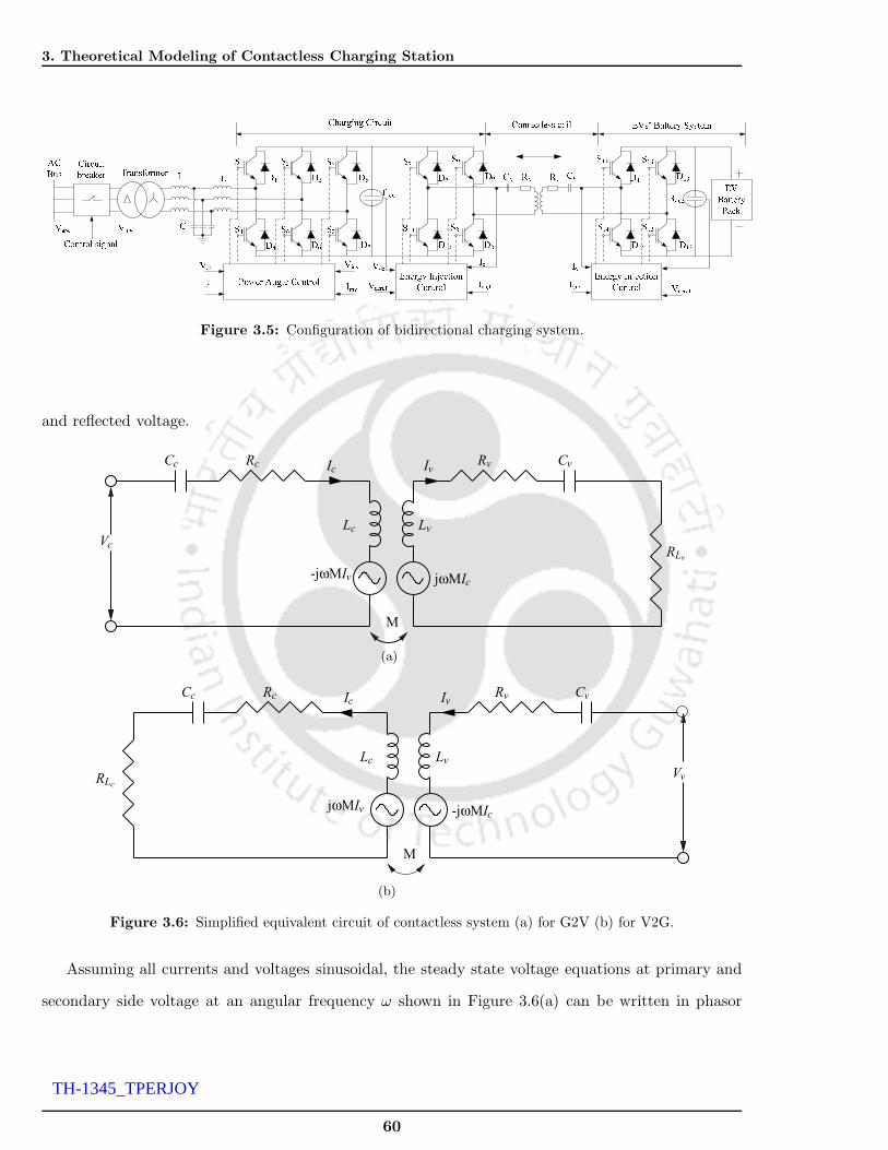
3. Theoretical Modeling of Contactless Charging Station
Figure 3.5: Configuration of bidirectional charging system.
and reflected voltage.
RLv
Rv
M
Cc Cv
Lc
Ic Iv
Lv
Rc
Vc
-jωMIv jωMIc
(a)
Rv
M
Cc Cv
Lc
-jωMIcjωMIv
VvRLc
Ic Iv
Lv
Rc
(b)
Figure 3.6: Simplified equivalent circuit of contactless system (a) for G2V (b) for V2G.
Assuming all currents and voltages sinusoidal, the steady state voltage equations at primary and
secondary side voltage at an angular frequency ω shown in Figure 3.6(a) can be written in phasor
60
TH-1345_TPERJOY

3.3 Bidirectional contactless charging system
form as given by (3.1) and (3.2).
Vc,1 =Ic,1
jωCc,1+ Ic,1Rc,1 + jωLc,1Ic,1 − jωM1Iv,1 (3.1)
jωM1Ic,1 = Iv,1Rv,1 + jωLv,1Iv,1 + Iv,1RLv,1 +Iv,1
jωCv,1(3.2)
In equation (3.1)- (3.2), Vc,1, Vv,1, Ic,1 and Iv,1 are the rms voltage and current of the 1st charger
circuit and the vehicle side circuit in the charging system. Cc,1 and Cv,1 are the series resonant
capacitors in the charger and vehicle side circuit. Similarly, Rc,1, Lc,1, Rv,1 and Lv,1 are the coil
resistance and self inductance of the charger and the vehicle side circuit respectively. M1 is the
mutual inductance of the contactless transformer in the charging system and is given by (3.3). RLv,1
denotes the EV battery and additional power electronics of vehicle during G2V operation and RLc,1
denotes the grid impedance and additional power electronics during V2G operation and K1 is the
inductive coupling factor between the primary and secondary coil. .
M1 = k1
√Lc,1Lv,1 (3.3)
Simplifying the above equations, the current of the contactless coil at the vehicle side is given by (3.4),
where Zv,1 is the approximated secondary side coil impedance.
Iv,1 =jωM1Ic,1Zv,1
(3.4)
Zv,1 = Rv,1 +RLv,1+ jωLv,1 +
1
jωCv,1(3.5)
The EV battery is considered as a load during G2V operation and it consumes power from the charger
circuit. The voltage reflected to the charger circuit is described by (3.6), where Zrc,1 is the transformed
impedance or the reflected impedance as seen from the charger circuit.
Vr,1 = Zrc,1Ic,1 (3.6)
Zrc,1=
−ω2M12
Zv,1(3.7)
Therefore, the current in the charger circuit is given by (3.8), where Zt,1 is the total impedance seen
from the charger circuit.
Ic,1 =Vc,1
Zt,1(3.8)
61
TH-1345_TPERJOY

3. Theoretical Modeling of Contactless Charging Station
Zt,1 = Rc,1 + jωLc,1 +1
jωCc,1+ω2M1
2
Zv,1(3.9)
To achieve high efficiency at the output of the charging system, the charger circuit and the EV battery
system should be operated at resonance frequency, therefore,
ωo =1√
Lc,1Cc,1
=1√
Lv,1Cv,1
.........1√
Lc,1Cc,1
=1√
Lv,nCv,n
(3.10)
The compensation capacitance at the charger circuit and the vehicle side is given by (3.11) and (3.12).
Cc,n =1
ωo2Lc,1
=1
ωo2Lc,2
......1
ωo2Lc,n
(3.11)
Cv,n =1
ωo2Lv,1
=1
ωo2Lv,2
.......1
ωo2Lv,n
(3.12)
The compensation capacitance (Cc,1) in the charger circuit is chosen such that the impedance seen
from the high frequency inverter (supply side) is purely resistive in nature. That is, it has to cancel the
reactive element and should have minimum VA rating i.e., the input voltage and current are in phase
with each other. The secondary compensation (Cv,1) is to increase the power transfer capability.
The choice of resonance capacitor in the charging circuit ensures, the impedance of the secondary
circuit (Zv,1), the reflected impedance (Zrc,1) seen from the charger circuit and the net impedance
seen by the power supply (Zt,1) are purely resistive in nature at resonance frequency ω = ωo. Similar
procedure described from (3.1) and (3.12) can be used to analyze the steady state behavior during
V2G operation.
3.4 Problem description
The modeling of multiple charging system in a CS and its coordination with grid is a challenging
task. This is because the EVs arrived in the CS may perform charging as well as discharging operation.
Moreover, the grids condition will not always suitable to exchange the power with the CS. Hence, the
study on managing multiple EV in a CS is a major issue, which has to be addressed. Therefore, the
main objectives of the work are:
• To develop component level multi-point charging (BCPT) system.
• To develop the suitable control strategy required to schedule the CS and to control the power
flow between the charging system and the grid.
62
TH-1345_TPERJOY

3.4 Problem description
3.4.1 Charging station control strategy
A reclosing control have been used in the CS to schedule the charging and discharging operation of
EVs. It connects the charging system lines through parallel connected ac bus to share energy among
EVs in the CS. Reclosing control obtains arrival time (ta), SOC status and departure time (td) as
its input parameter and assign the charging systems for EVs arrived in the CS. The reclosing control
has used a scheduling algorithm for charging system assignment. The control process involved in
reclosing control is described in Figure 3.7. This explains the scheduling process to manage multiple
EVs arrived in the CS. An EV owner can specify his planned departure time or leave it undefined,
if he doesn’t have a departure deadline. Thus, EV owner can request a specific charging/discharging
depending on the actual parking time or departure time. If the grid is identified to be unsuitable to
exchange power between the charging system lines, it disconnects the charging system line by opening
the circuit breaker (CB).
3.4.2 Scheduling algorithm
A scheduling algorithm has been developed in the reclosing control to manage the EVs arrived
in the parallel connected charging systems. It identifies the SOC status of each EVs in the CS and
makes the charging system assignment depending upon the vehicle check-in and thus guarantee a
certain amount of energy that one EV will be provided from the other one. An EV arrived to support
the grid and an EV arrived to charge will be allocated depending on the time of arrival. The reclosing
control keeps every update about the EV arrived in the CS and assigns the charging systems. If
several request are received , the controller gives preference to the earliest request and suitable vehicle
will be allocated fast. Thus, SOC levels and charging/discharging time are specified to each charging
systems and the controller. In a particular case, if all EVs arrived in the CS is found to either charge
or discharge its EVs, then the CS checks the grids condition and allows the EVs to charge or discharge
from the grid. A request from EV owner will be rejected under two cases: if all EVs arrived in the CS
is to charge and the grids condition is already in peak-hour period or if all EVs arrived in the CS is to
discharge and the grids condition is off-peak hour and cannot accept any power support from the CS.
Then the EV owners are unable to share its energy and will have to leave the CS. Figure 3.7 shows
the flow chart of scheduling process in reclosing control to schedule EVs in the CS.
Assuming, four EVs (EV1, EV2, EV3 and EV4) have arrived at the CS with SOC levels 90%, 10%,
63
TH-1345_TPERJOY

3. Theoretical Modeling of Contactless Charging Station
Is
CS has
EVs for both
discharge
Inputs:
SOC status of EVs
minnimum SOC level
Indentify EVs with
perfrom energy sharing
yes
EV with minnimum
Connect maximum
SOC EV based
Is
discharge
charge/
level attained
max/minnim
user
limit
Start
EVs have arrived to
check
yes
check
yes
yes
connect EVs to grid
EVs leave the CS
Stop
discharge
connect EVs to grid
check all
EVs to
charge
yes
No
No
No
No
No
on ta
ta, td
charge &
Vg, f
with maximum &
VL > 400V
VL < 400V
Figure 3.7: Control operation of charging station.
85% and 15% at time t1, t2, t3 and t4 to both charge and discharge its EVs. The time interval has been
considered as t4 <t3 <t2 <t1. The reclosing control finds the EV arrived at the earliest and its SOC
status. It also checks the next arrived EV. Here, in this case it assigns EV1 to discharge its energy to
support EV2. It interconnects the charging points CP1 and CP2 to share the energy demand between
64
TH-1345_TPERJOY

3.4 Problem description
EV1 and EV2. Likewise, it interconnects EV3 to EV4 depending on the time of arrival and SOC status.
The maximum and minimum SOC levels the EVs should charge and discharge is defined by the EV
owner’s depending on which the controller assigns the charging systems. An EV owner also defines the
SOC limit to which an EV have to perform the charge/discharge operation. For convenience sake, the
reclosing developed in this work has considered the maximum SOC to be greater than or equal to 70%
and and minimum SOC to be less than or equal to 20% and the charging systems are assigned based
on the time of arrival. The energy sharing takes place between the selected EVs in the CS through
ac bus network. If suppose the initially allocated EV cannot fulfill the energy demand of other EV,
the controller reassign or reallocate another possible EV to fulfill the minimum charging/discharging
requirement as per the CS standard. In a situation, if the controller cannot assign suitable EVs to
share its energy or to exchange power with grid, the EV owners will have to wait till the arrival of
next EV or will have to leave the CS.
3.4.3 Charging (BCPT) system
To analyze multiple EVs arrived in the charging system and to examine its power flow capability,
ten component level charging systems are modeled in the simulation environment. The circuit topology
for single charging system is shown in Figure 3.5. The charging systems are able to operate in
two modes: G2V operating mode and V2G operating mode. This section has detailed the circuit
arrangement and its bidirectional power transfer during G2V and V2G operation.
3.4.3.1 G2V operation
EVs are scheduled to charge their batteries through any parallel connected charging system con-
nected with high SOC batteries or it can be charged from the utility grid during off-peak hours. EVs
are connected to the power supply through three phase converters (S1 - S6) present in the charging
system. Therefore, the two systems should be properly synchronized and controlled to transfer the
power from one system (sender) to the other (receiver) system. For this reason, the charging system
is controlled using power angle control shown in Figure 3.8. It takes sender systems’ voltage as its
reference and controls the three phase converter switches (S1 - S6) to transfer power from sender to
the receiver system. The power angle control has three phase PLL block and a fuzzy logic controller
(PA-FLC) as shown in Figure 3.8. It takes the reference voltage, frequency and current from sender
and receiver system. Initially, both the system is synchronized based on the sensed information and
65
TH-1345_TPERJOY

3. Theoretical Modeling of Contactless Charging Station
Three phase
PLL
conversion PA−FLC
component
symmetric
extraction
dqo
abc
comparator
signal 4kHz
carrier
dqo
p.u
abc
Er
∆Er
δ
S1
S6
δ′
ωt
Vinv
Iinv
Vg
Pr
Pm
V ∗abc
to
ddt
αβ
Figure 3.8: Power angle control.
the system is interconnected. Power angle control senses the grid voltage directly and tracks the
phase and frequency variations of the utility grid. In this system, the three phase utility voltage can
be represented by (3.13).
Vg = Vabcn =
[sin (θ) sin
(θ − 2π
3
)sin
(θ +
2π
3
)]T
(3.13)
where,
Vabcn = [Van Vbn Vcn]T (3.14)
The voltage equation (3.13) can be transformed to the d-q axis frame as given by (3.15).
Vqdo = TsVabcn (3.15)
where, Ts is the transformation matrix and is given by (3.16).
Ts =2
3
sinωt sin(ωt− 2π3 ) sin(ωt+ 2π
3 )
cosωt cos(ωt− 2π3 ) cos(ωt+ 2π
3 )
12
12
12
(3.16)
The Vqdo given in (3.16) is obtained from three phase grid voltage. The frequency of each phase
is extracted from the grid voltage and this will be same for all the three phases. The power (Pm) has
been calculated from the output of the three phase bidirectional converter by sensing its voltage and
66
TH-1345_TPERJOY

3.4 Problem description
current. Measured (Pm) and reference power (Pr) are given as input to PA-FLC. Error (Er) and error
rate (∆Er) is estimated based on the measured (Pm) and the reference power (Pr). The PA-FLC
calculates the required power angle (δ). Using the power angle, the new symmetrical components are
extracted and the required three phase reference voltage is obtained using equation (3.17).
vabc′ = TmVqdo (3.17)
where, Tm denotes the new transformation matrix and is given by (3.18).
Tm =2
3
sin(ωt+ π6 − δ) cos(ωt+ π
6 − δ) 1
sin(ωt− π2 − δ) cos(ωt− π
2 − δ) 1
sin(ωt+ 5π6 − δ) cos(ωt+ 5π
6 − δ) 1
(3.18)
The three phase reference voltages are generated and pulses are produced using sinusoidal pulse
width modulation (SPWM) technique. Thus, during G2V operation the bidirectional three phase
converter acts as a rectifier and converts three phase ac voltage to dc. This converter is cascaded with
the next converter (S7 - S10), which converts dc to high frequency ac current in the primary winding.
Because of the mutual coupling between the primary and secondary coil, the required power transfer
on the secondary side can be regulated by controlling the high frequency ac current in the primary
coil through switches (S7 - S10). The circuit operation is based on the principle of resonance [109].
When the switches (S7 - S8) is controlled to be on, the source voltage is injected into the primary
coil in positive direction. When the current falls to zero, the switches (S9 - S10) is on in the reverse
direction. The controller present in the primary side converter maintains a high frequency ac current
in the secondary side. As the coils are magnetically coupled through M , the secondary side converter
switches (S11 - S14) converts high frequency ac current to dc and regulates the amount of power
extracted from the primary coil to meet the vehicle demand. In many cases, a bidirectional dc-dc
converter is also employed at the secondary side to regulate the output voltage to regulate the vehicles
of different voltage and current ratings. The pattern of membership function of PA-FLC is shown in
Figure 3.9 and its rule base is given in Table 3.1.
67
TH-1345_TPERJOY

3. Theoretical Modeling of Contactless Charging Station
1
0.50
−1 −0.5 0 0.5 1
NB NS Z PS PB
Er/∆Er (p.u)
(a)
1
0.50
22.5 45 9011.25
VL L M H VH
67.5
δ′(degree)
(b)
Figure 3.9: Membership function of phase angle-fuzzy control (PA-FLC) (a) Input: error and error rate (Er/∆Er) (b) Output: Power angle (δ′).
Table 3.1: Rule base of power angle control (PA-FLC)
Er/∆Er NB NS Z PS PB
NB VL L M H VH
NS VL L M H VH
Z VL L M H VH
PS VL L M H VH
PB VL L M H VH
Five fuzzy subsets such as Negative Big (NB), Negative Small (NS), Zero (Z), Positive Small (PS)
and Positive Big (PB) are chosen as input membership function and for the output Very Low (VL),
Low (L), Medium (M), High (H) and Very High (VH) are chosen in order to obtain required control
action. Triangular membership functions are used as it is simpler and easier to implement.
3.4.3.2 V2G operation
During V2G operation, the secondary side converter switches (S11 - S14) converts EVs battery
voltage to high frequency ac current to feed the contactless coils. This works on the principle of
resonance as described above. The required power flow in the charging circuit side is regulated
using the controller present in the vehicle side converter. As the vehicle side coil inductance (Lv) is
magnetically coupled to the charging circuit side coil inductance (Lc), the high frequency ac current
will get induced in the charging circuit. Further, the primary side converter acts as an inverter (S1
- S6) to convert dc to three phase ac. Thus, the power is transferred in the reverse direction using
bidirectional switches in the converter. The amount of power supplied from the vehicle (sender) is
decided by the power angle control explained above. The maximum power that can be transferred is
at an angle δ = 90
68
TH-1345_TPERJOY

3.4 Problem description
3.4.4 Design of critical parameters
3.4.4.1 Filter circuit
Figure 3.10 shows the equivalent circuit of three-phase bidirectional converter connected to the grid
through an isolation transformer. The switching frequency effects in the converters of the charging
station can inject harmonics to the grid. These harmonics requires the connection of low pass filter
between the inverter and the grid. The filter attenuates most low order harmonics in the output.
The inductor (L) determines the ripple in the current and reduces the low frequency harmonic
components. The voltage across the filter component (Vdc) with respect to the switching frequency
(fsw) and ripple current (∆I) is given by (3.19).
Vdc= L∆Iconvfsw (3.19)
According to the harmonic standards, 15-20% of the rated ripple current is allowable; 20% is assumed
LgRg L fL
C
Grid network transformer LC filter
Vgrid
Vconv VdcVgrid
3 ϕ ac-dc
Cdc
Figure 3.10: Equivalent circuit of grid connected inverter.
in this study. The maximum ripple depends on the inductance, dc voltage (Vdc) and fsw. The dc link
voltage and switching frequency is constant and the inductance can be calculated using (3.20).
L =1
8
Vdc
∆ILfsw
(3.20)
The high frequency components have to be eliminated from the inductor current when connected to
the grid. This must be performed by the shunt impedance which is low at high frequencies. Assuming,
Vconv is the charging system voltage, Iconv is the charging system current and C, Ltf , Lg and L are
the capacitor, inductance of the transformer and grid network and filter inductor respectively, then
the ratio of Iconv to Vconv is given by (3.21).
69
TH-1345_TPERJOY

3. Theoretical Modeling of Contactless Charging Station
Iconv
Vconv=
1
s3LC(Lg + Ltf ) + s2LRgC + s(L+ Ltf + Lg) +Rg(3.21)
C =Vconv
Iconv− s (L+ Ltf + Lg) −Rg
s3L (Lg + Ltf ) + s2LRg(3.22)
3.4.4.2 Dc link capacitor
The three phase ac-dc converter in the charging system is made of bidirectional switches, which
converts three phase phase ac-dc conversion in the forward direction and dc-ac conversion during
reverse power flow. During charging operation, the peak-to-peak dc output voltage of the rectifier
contains harmonics in the output voltage and that can be written as given by (3.23) [110]. While in
case of reverse operation, this capacitor acts as a dc link capacitor.
Vdc(pp) =Vm
2fZLCdc
(3.23)
where Vm is the maximum peak value, f is the input side frequency, ZL is the load impedance and
Cdc is the filter capacitance. The ripple factor (RF) can be determined from the RMS and average
output voltage, which can be expressed as given by (3.24).
RF =1√
2(4fZLCdc − 1)(3.24)
From the above equation Cdc can be solved as given by (3.25).
Cdc =1
4fZL
(1 + 1√
2RF
) (3.25)
3.5 Simulation results
The CS described in the previous section has been tested in simulation environment. In order to
verify its functioning, a 500kVA capacity CS has been modeled with ten parallel connected charging
system fed from 440Vrms, 50Hz ac bus network. The circuit topology used for charging system is
shown in Fig. 3.5. The contactless coils are fed by high frequency inverter. The secondary side of the
coil is connected to 300V EV battery. The circuit parameters of the charging systems are given in
Table 3.2. The primary and secondary side of the coils are magnetically coupled at a coupling factor of
0.2537. For ease of analysis, EVs batteries are divided into five groups based on the terminal voltage
(V), energy (kWh) and SOC levels. To avoid repetition the results are shown only for five sets of EVs
70
TH-1345_TPERJOY

3.5 Simulation results
batteries.
Table 3.2: Simulation parameters of charging system.
Parameter Description Values Parameter Description ValuesCc, Cv compensation 1.17µF , 1.17µF Lc, Lv Coil 34.8µH, 34.8µH
capacitance inductanceM mutual 8.83 µH Rc, Rv coil 433 µΩ
inductance resistancek coupling 0.2537 Cdcc
dc link 100mFfactor capacitor (charger) -
LCL LCL 600µF , 80µF , Cdcvdc link 180µF
filter 800µF capacitor (vehicle)
For convenience of analysis, the following assumptions are made in this work:
• Each charging systems are designed for a maximum power handling capacity of 50kW.
• The EVs batteries are not allowed to discharge below 20% SOC level and the charging level is
limited to 85% SOC.
The parameters of EV battery are given in Table 3.3.
Table 3.3: Parameter of EV battery.
EVs Voltage Energy SOC Er Ea
(V) (kWh) (%) (kWh) (kWh)EV1 to EV2 300 40.2 15 11.9 -EV3 to EV4 300 42.6 94 - 13.22EV5 to EV6 300 47.4 81 - 11.36EV7 to EV8 300 54.6 19 19.14 -EV9 to EV10 300 64.2 98 - 28.28
In Table 3.3, there are 3 sets of EVs to discharge its energy and two sets of EVs arrived to charge.
The charging systems with high SOC batteries are allowed to discharge its energy to support the
charging system with low SOC EVs. However, EV9 cannot be scheduled in the charging system, as
the charging systems are already interconnected. This can be connected to grid and therefore EV9 is
allowed to discharge its energy to support the grid. Figure 3.11 shows the battery power of five EVs
arrived in the charging system for two hour period. Among this, EV3 and EV5 discharges its energy
to support EV1 and EV7. EV9 discharges its energy to support the grid.
71
TH-1345_TPERJOY

3. Theoretical Modeling of Contactless Charging Station
10 : 00 10 : 15 10 : 30 10 : 45 11 : 00 11 : 15 11 : 30 11 : 45 12 : 00−30
−25
−20
−15
−10
−5
0
5
10
15
20
Time (hrs)
Bat
tery
pow
er (
kW)
EV
1EV
3EV
5EV
7EV
9
−5.68
−6.61
9.19
−14.14
5.77
Figure 3.11: Power supplied from the EVs batteries.
Figure 3.12 shows the SOC levels of five EVs, after charging/discharging operations in the CS for
two hours. EV3, EV5 and EV9 has arrived in the charging system with high SOC batteries and has
discharged its energy. EV1 and EV7 has arrived in the charging system with low SOC batteries to
charge its batteries.
10 : 00 10 : 15 10 : 30 10 : 45 11 : 00 11 : 15 11 : 30 11 : 45 12 : 00
20
40
60
80
100
Time (hrs)
Sta
te o
f Chr
age
(%)
EV
1EV
3EV
5EV
7EV
9
SOCini
= 98 %
SOCini
= 94 %
SOCini
= 81 %
SOCini
= 19 %
SOCini
= 15 %SOC
fin = 49.41 %
SOCfin
= 71 %
SOCfin
= 66.01 %
SOCfin
= 69.56 %
SOCfin
= 76.44 %
Figure 3.12: SOC levels of EVs.
The charging and discharging current of five sets of EVs shown in Figure 3.13. The positive
current curves denotes EVs arrived in the charging system is performing charging operation and
72
TH-1345_TPERJOY

3.5 Simulation results
negative current denotes EVs are discharging its energy to support other EVs or to support the grid.
10 : 00 10 : 15 10 : 30 10 : 45 11 : 00 11 : 15 11 : 30 11 : 45 12 : 00−100
−80
−60
−40
−20
0
20
40
60
Time (hrs)
Bat
tery
cur
rent
(A
)
EV
1EV
3EV
5EV
7EV
9
−56.57
−22.09
23.84
−26.43
36.75
Figure 3.13: Charging and discharging current of EVs.
Figure 3.14 show the charging system voltage at the terminals of the bus bar. The positive and
negative power represents the power flow in two directions. The amount power flow is decided by the
user and controlled by the charging system.
0 0.4444 0.6667 0.8889 1.1111 1.3333 1.5556 1.7778 2−20
−15
−10
−5
0
5
10
15
Time (hrs)
Cha
rgin
g po
int p
ower
(kW
)
EV7
EV1
EV5
EV3
EV9
5.95
−6.41
−5.57
9.57
−13.58
Figure 3.14: Power at the charging point.
Figure 3.15 show the node voltage and node current at the terminals of the CS. Figure 3.16 shows
the distribution node power.
73
TH-1345_TPERJOY

3. Theoretical Modeling of Contactless Charging Station
10 : 00 10 : 15 10 : 30 10 : 45 11 : 00 11 : 15 11 : 30 11 : 45 12 : 000
100
200
300
400
500
Time (hrs)
Nod
e vo
ltage
(v)
and
cur
rent
(A
)
DN voltage
DN current 49.59
440.25
Figure 3.15: Node voltage and node current.
10 : 00 10 : 15 10 : 30 10 : 45 11 : 00 11 : 15 11 : 30 11 : 45 12 : 000
5
10
15
20
25
30
Time (hrs)
Nod
e po
wer
(kW
)
DN Power −21.83
Figure 3.16: Power at the distribution node.
3.6 Conclusions
In this chapter, a CS has been modeled using multiple parallel connected charging (BCPT) systems.
The theoretical operation of the parallel connected BCPT systems has been analyzed for G2V and
V2G operation. The individual charging system are controlled to control the power flow in both the
direction. A control strategy has been used to schedule the charging/discharging operation of multiple
EVs in the CS. A 500 kVA multiple BCPT system is modeled in the simulation environment and the
validation of the study has been carried out using five EVs batteries of different ratings.
The contactless charging system modeled in this chapter has considered a fixed coupling coefficient;
74
TH-1345_TPERJOY

3.6 Conclusions
but in realtime the coils can be misaligned and its coupling coefficient may change because of uneven
surface impacts, due to heavy battery weights and roads. This necessitates the need to compute
MI between two coils with its misalignments. The next chapter discusses an analytical approach to
compute MI between two coils including lateral and angular misalignments.
75
TH-1345_TPERJOY

3. Theoretical Modeling of Contactless Charging Station
76
TH-1345_TPERJOY

4Computation of Mutual Inductance for
Contactless System
Contents
4.1 Introduction . . . . . . . . . . . . . . . . . . . . . . . . . . . . . . . . . . . . 79
4.2 Possible variations of square coils . . . . . . . . . . . . . . . . . . . . . . . . 81
4.3 Analytical modeling of square coil . . . . . . . . . . . . . . . . . . . . . . . 83
4.4 Finite element modeling of square coil . . . . . . . . . . . . . . . . . . . . . 86
4.5 Experimental verification . . . . . . . . . . . . . . . . . . . . . . . . . . . . . 88
4.6 Numerical results and discussion . . . . . . . . . . . . . . . . . . . . . . . . 92
4.7 Conclusions . . . . . . . . . . . . . . . . . . . . . . . . . . . . . . . . . . . . . 99
77
TH-1345_TPERJOY

4. Computation of Mutual Inductance for Contactless System
78
TH-1345_TPERJOY
4.1 Introduction
Abstract
This chapter presents an analytical approach for computing the mutual inductance between two air
core square coils placed in a flat planar surface. The mutual inductance of the coils is calculated for all
possible variations including lateral and angular misalignments in space. In contrast to conventional
approximated formulae, the straightforward approach based on Biot-Savart principle is used and their
integrals are computed numerically. The results of computed mutual inductance by analytical method
are validated by finite element analysis and an experimental setup. Finally, the analysis compares
the three mutual inductance calculations: an analytical method, the finite-element model and an
experimental results. The values computed by three methods in all cases are in good agreement.
The work presented in this chapter is published in [30].
4.1 Introduction
The computation of mutual inductance (MI) between two coils is a classical problem in electrical
engineering and that remains important to this day for a wide variety of physical disciplines [111].
Some important applications such as transcutaneous transformers, coil guns, linear motors, contactless
based electric vehicle charging systems etc., are modeled with inductively coupled circuits such as
transformers and contactless power transfer (CPT) systems [36,48,112–114]. Recent developments in
CPT systems have prompted more the requirement to investigate the MI of the coil [22, 23, 70]. The
design of contactless coils in BCPT systems are very complex as the coils are usually misaligned due
to variations in the system and worsen the coupling between the coils [69, 70]. These misalignments
could cause fluctuations in the output voltage and affects the stability of the system [113]. Therefore,
the computation of MI with all its lateral and angular misalignments must be fully addressed, which
is the first step for studying the characteristics of such systems.
A survey of past literature shows that, Grover’s tabular data remains the most standard for
calculating the MI for a wide variety of coils and wire forms [115–119]. However, its use has mostly been
restricted to zeroth and first-order calculations and it is proved to be inaccurate for loosely coupled
and short coils [116–119]. Several contributions for MI computation are found in the literatures
[115, 117–126]. In some work, MI is calculated by means of approximated formulae [116, 120, 121],
Heuman’s lambda function [111, 122–124], Bessel and Struve functions [125, 126] and in other works
using Biot-Savart law [127, 128]. However, much of the earlier works are devoted for circular and
79
TH-1345_TPERJOY

4. Computation of Mutual Inductance for Contactless System
coaxial coils [111, 116–126]. These coil geometries are well suited for fixed coil systems and they are
not tolerant for misalignments in the coils. Square and rectangular coil geometries are found to be
well suited for mid-distance CPT systems; as they show better tolerance for misalignments [36, 129].
Although, there are numerous works carried out in this area, only very few work have studied these
coil geometries with its misalignment effects [22,23,36,69, 70, 114, 129–132]. In [69,70], an analysis is
presented based on rectangular coil geometry. However, these works mainly focused on the design of
charger based on resonant magnetic coupling to transfer power wirelessly over a long distance. It has
been observed from the literature, the effects of misalignments of the coils have not been investigated
in detail from both geometrical stand point and circuit design stand point.
This chapter describes an analytical approach to compute the MI between two coils. A detailed
investigation of all possible lateral and angular misalignments with horizontal and vertical variations
are presented. Square coil geometry has been chosen here to analyze the misalignments of the coils.
The proposed analytical approach is capable of calculating MI for all positions of the coil, thus reducing
complex mathematical equations. The results of the analytical model are compared with 3-D finite
element analysis (FEA) and an experimental setup. Figure 4.1 shows the main building blocks used
for MI computation. The coil which is excited is referred as excitation coil (EC) and the coil where
the output variations are observed is referred as observation coil (OC). The finite element results and
experimental evaluation justifies the accuracy of the analytical model in all cases.
SourceCoil (EC)
Contactless Path Observation
Coil (OC)
Excitation
Figure 4.1: Block diagram of contactless system.
For clear interpretation, the possible variations of square coils is presented in Section 4.1. The
analytical modeling of square coil is given in Section 4.2. Finite element modeling is addressed in
Section 4.3. Experimental verification is done in Section 4.4. Results are described in Section 4.5, this
section is followed by conclusions in Section 4.6.
80
TH-1345_TPERJOY

4.2 Possible variations of square coils
Perfectmisalignment
Both lateral andangular misalignment
variationVerticalvariation
Angle 20 Angle 30
Lateralmisalignment (LM)
Angle 10
Angular
Planar
alignment (PA)
Horizontalvariation
Planarvariation
Possible variations of square coils
Figure 4.2: Possible variations of contactless coils.
EC
OCh
(a)
EC
OC
θ
(b)
OCEC
d
h
(c)
OC
EC
θd
(d)
OC
EC
θ
h
(e)
EC
OC
d
hθ
(f)
Figure 4.3: Schematics of square coils for analyzed variations (a) PA - vertical variation (b) PA - planarvariation (c) LM - horizontal variation (d) LM - planar variation (e) angular misalignment (f) both lateral andangular misalignment.
4.2 Possible variations of square coils
The analysis presented in this chapter computes MI between two air core square coils, placed in
a flat planar surface coinciding in space. As the MI of the coil varies with the change in position
of the coils, different variations of the coils i.e., misalignments are analyzed throughout this chapter.
Different cases of variations of OC with respect to EC are taken into account, which are shown in
Figure 4.2 and its corresponding schematics are shown in Figure 4.3. The coil parameters used in this
work are described in Table 4.1.
81
TH-1345_TPERJOY

4. Computation of Mutual Inductance for Contactless System
Table 4.1: Coil parameters
EC, OC Excitation coil, observation coil
h deviated vertically from the center of the coil
d deviated horizontally from the center of the coil
θ Angle of OC with respect to EC
If the EC and OC are placed in a flat planar surface with coinciding axes, such arrangement of coils
is referred as perfect alignment (PA). Two types of variations like vertical and planar variation are
analyzed in this case as shown in Figure 4.3(a) and Figure 4.3(b). The flux linkage will be maximum
when OC and EC are perfectly aligned and the coils are close to each other. When OC is moved
vertically away from EC, the coupling between the coil changes and MI decreases. In planar variation,
EC and OC are placed near to each other and OC is rotated along its axis at various angle as shown
in Figure 4.3(b). As the distance between the coils is kept constant, the coil overlapping area doesn’t
vary much and due to this the variation of flux linkage in this case would be nominal.
There can be another misaligned case in real time systems, where the coils are situated in parallel
plane and displaced horizontally, such arrangement of coils is referred as lateral misalignment (LM).
This type of misalignment is observed for different horizontal distances between the axes of the coils.
For LM, horizontal and lateral variations are studied which are shown in Figure 4.3(c) and Figure
4.3(d). The flux linkage and MI of the coils depends on the distance of OC from EC and it would
drop when it moves away from the EC. Apart from this, there can be a situation where OC can be
titled up or down with certain angle (0 to 90) due to unequal surface impacts; such arrangement of
coils is referred as angular misalignment which is shown in Figure 4.3(e). In similar way, there can
be a general case where OC can be both tilted and varied horizontally, such arrangement of coils is
referred as both lateral and angular misalignments, as shown in Figure 4.3(f). In this misaligned case,
MI depends on both the tilted angle and horizontal distance. The misalignments described above are
calculated using an analytical approach and are validated by both FEA models and an experimental
setup. The details of evaluation methods, its results and comparison are explained in later sections.
82
TH-1345_TPERJOY

4.3 Analytical modeling of square coil
4.3 Analytical modeling of square coil
4.3.1 Modeling of mutual inductance
The circuit topology of the two coupled coils EC and OC resembles an inductively coupled trans-
former, which is represented by an equivalent circuit as shown in Figure 4.4.
M
EC OC
Source
I
VO
Figure 4.4: Equivalent circuit model of an inductive coil.
Consider EC and OC placed near to each other as shown in figure. When EC is connected to the
power supply, current (I) flows in it, which produces a magnetic flux (λ1) and a part of the flux (λ12)
links with the secondary side coil OC. Then, the MI of the coil is represented as M and is given by
(4.1).
M =λ12
I(4.1)
The flux linked with the OC due to current in the EC can be calculated analytically by considering
the flux distribution of each individual coil turns of the OC. The method works by approximating the
area of OC with small regions, encompassing the entire square and thereby considering the complete
spiral square coil. The flux through each small region of the OC is taken into account to calculate
the flux linked to OC due to EC. To carry out this process, a sequence of program routine have been
used. The total flux linked in the OC is obtained by the sum of the flux linked in each small grid for
all the turns of the OC. Assuming ϕn is the flux linked with the nth region of the area enclosed by
single turn of the OC, then λ12 can be estimated by (4.2). The limit of the summation depends on
83
TH-1345_TPERJOY

4. Computation of Mutual Inductance for Contactless System
the number of small regions formed in a single turn of OC.
λ12 =∑
ϕn (4.2)
The flux linked to each of these small regions of OC due to EC is calculated with the following
assumptions.
• The insulated coil conductors are placed such that there is no space between conductors of any
two loops and they are touching each other.
• The magnetic field in the small region of OC caused due to EC (Figure 4.5(b)) is assumed to be
constant and its value is calculated at the center of that small region.
Having made the above assumptions, ϕn for each small region is calculated using (4.3) and (4.4),
which depends on the magnetic field at the center (−→Bc) of the small region, nth area (An) and normal
vector of the nth area (An).
ϕn =−→Bc · (An · An) (4.3)
An = ∆xn · ∆yn (4.4)
Here, ∆xn and ∆yn are the length and width of the small divided region as shown in Figure 4.5(b).
The magnetic field−→Bc at the center of the small region is caused due to EC.
−→Bc is calculated for P
turns of EC and is given by (4.5). The individual coil turns of EC is modeled by four straight current
carrying conductors. Let−→B is the magnetic field due to one current carrying loop of EC as shown in
Figure 4.5(a) and is given by (4.6).
−→Bc =
P∑
m=1
−→B (4.5)
−→B =
4∑
n=1
−→Bn (4.6)
In the above equation, n represents the four sides of the single current carrying loop and−→B1,
−→B2,
−→B3 and
−→B4 are the magnetic fields of the sides of the square coil AB, BC, CD and DA.
−→Bn can be
calculated from the Bio-Savart law for magnetic field. The basic magnetic field equation (−→Bn) at any
point in space due to a straight current carrying conductor is given by (4.7).
−→Bn =
∫µ0I
−→ds× R
4πR2(4.7)
84
TH-1345_TPERJOY

4.3 Analytical modeling of square coil
The vector R, in the above equation is the unit vector in the direction of position vector of the
observation point, originating from the differential element of current carrying conductor (−→ds). The
direction of−→ds is in the direction of current in the conductor. The integration in (4.7) is performed
over the length of the conductor. Similarly, the magnetic field at a point in space and flux linkage
calculations can be done for spiral square coils with multiple turns as shown in Figure 4.5(c), where
L and W are the length and width of the coil.
C
−→B4
−→B3D
A B−→B1
−→B2
(a)
An∆Xn
∆Yn
D
A
C
B
flux linkage (ϕn)
(b)
W
L
(c)
Figure 4.5: Square current carrying coil (a) single turn (b) single turn segmented (c) multiple turn.
4.3.2 Numerical evaluation
The MI for the mutually coupled coils is calculated numerically using the equations discussed in
the previous section. The procedure for numerical calculation is explained in the following steps.
• The total number of turns for EC (P ) and OC (Q) are determined.
• 3D co-ordinates of a single turn of EC and OC are determined.
• Diameter of conductor and distance between EC and OC (depending on the type of variation)
is determined.
• The selected turn of the coil is divided into multiple small areas from A1.....An as shown in
Figure 4.5(b).
• Calculate the total flux linked to each small region of OC using (4.8) by calculating the magnetic
field at the center .
ϕ1 =4∑
n=1
µ0
4π
∫I−→ds× R1
R21
·(A1 · A1
)(4.8)
85
TH-1345_TPERJOY

4. Computation of Mutual Inductance for Contactless System
• The flux linked in a single turn (ϕm) of OC is obtained by summing all the fluxes using (4.9).
ϕm =P∑
k=1
∑(ϕ1 + ϕ2...... + ϕn) (4.9)
• This procedure is repeated for all turns of EC and OC and λ12 is calculated using (4.10).
λ12 =
Q∑
m=1
ϕm (4.10)
• Therefore from these equations MI is calculated using (4.1).
The detailed description of this evaluation is given in the flowchart shown in Figure 4.6. This
procedure has been used for all variations of EC and OC with their corresponding new coordinates
and vertices. Thus, the method adapted in this work has used only Biot-Savart law for a straight
current carrying conductor; which is the basic equation for calculating the magnetic field. It does
not require any double or triple integration functions for its computation. This gives an interesting
compactness for the calculation of MI by avoiding complicated mathematical equations. An example
for particular case of variations is given in Appendix (see Appendix A.5).
4.4 Finite element modeling of square coil
The commercial 3-D finite element tool ANSYS Maxwell 14.0.0 has been used for validating the
analytical model. The EC and OC considered in this work have 11 and 9 turns respectively. The EC
is excited with a current of 10A. The EC and OC are modeled for different variations and are analyzed
by changing their co-ordinates in simulation environment. To simplify the analytical calculations and
to reduce the computation time, following assumptions are made in this investigation for flux linkage
calculations.
• As the 3-D FEA model for spiral square coil takes very long time and sophisticated computation
environment, the models are analyzed with all the dimensions reduced to one fifth of the original.
This adjustment is justified as the variation of the flux linkage is linear with the dimension of
the whole system, which can be proved analytically.
• To reduce the computational time, OC is put as a surface whose area is equal to that of EC and
flux linked to the surface has been calculated.
86
TH-1345_TPERJOY

4.4 Finite element modeling of square coil
Start
Divide the selected turn of OC into
small equal region
Select one turn (k) from P turns of EC
Calculate−→
Bc at the center of each small
Calculate ϕm linked in a single
k = P
yes
m = Q
m = m+1
yes
linked to
all Q and P turns of OC and EC
Determine the total flux (λ12)
Stop
k = k+1
Determine coordinate, vertices and distance
Select one turn (m) from Q turns of OC
no
no
region due to selected turn of EC using (4.5)
turn of OC using (4.8) and (4.9)
Compute M using (4.1)
Figure 4.6: Flowchart describing the numerical evaluation.
• The multiple turns of EC and OC are assumed to be placed near with no space between the
turns of the coils.
The models are created using the co-ordinates taken from the experimental setup. The FEA
models are formed for all the configurations of the coils and various positions of OC by changing its
coordinates. Figure 4.7 shows the FEA models of the coils for different variations such as vertical,
87
TH-1345_TPERJOY

4. Computation of Mutual Inductance for Contactless System
angular and planar.
(a) (b) (c)
Figure 4.7: FEA models of square coils for different variations (a) vertical (b) angular (c) planar.
The flux linked in the OC due to EC is found by integrating the magnetic field over the area of
OC using Maxwells field calculator. To ease the calculations script files are recorded and used for all
the models. This type of coil arrangement and usage of script files is more convenient and simple to
evaluate the flux linked in the OC. This avoids creating the model every time for various angles or
distance. Figure 4.7(a) shows the side view of the vertical variation of the square coil at a particular
distance. The fan shaped arrangement shown in Figure 4.7(b) is the side view of the angular variation
of the coil. Here the OC is placed for a range of angles from 0 to 90 at an interval of 10 at certain
vertical height. Figure 4.7(c) depicts the top view of OC placement of planar variation rotated along
its axis at various angles. The angle between two adjacent positions of OC is 15. Figure 4.8 shows the
2D plot of magnetic field lines of EC and OC having four conductors each. Figure 4.8(a) shows two
positions of vertical variation of OC at small and large distances. Figure 4.8(b) shows two positions
of angular variation of OC at 0 and 45 angles. As it can be seen from the plots, the magnetic field
lines crossing the OC are less when the coils are away as compared to the coils placed near to EC.
4.5 Experimental verification
In order to verify the analytical and FEA results an experimental setup is built in the laboratory.
The circuit topology and its control blocks are shown in Figure 4.9 and Figure 4.10. Table 4.2 shows
the specifications of the components used for evaluation.
88
TH-1345_TPERJOY

4.5 Experimental verification
(a) (b)
Figure 4.8: Magnetic field lines for cut section of coils (a) vertical (b) angular
Table 4.2: Specifications of the components
symbol Description Values
Vdc DC supply 0-30V
Lp Inductance of EC 54µH
Ls Inductance of OC 37µH
f Frequency 18kHz
Cf Filter capacitor 1.44µF
W Width of the coil 18cm
L Length of the coil 18cm
Np Number of turns in EC 11
Ns Number of turns in OC 9
4.5.1 Description of power circuit and control circuit
The coils are accommodated in the flat planar surface without overlapping each other. The exci-
tation circuit is made of a simple MOSFET based converter to convert dc voltage to high frequency
ac voltage. The LC tank circuit shapes the voltage waveform and obtains an alternating voltage of
resonant frequency across the coil to produce a variable magnetic field. The harmonics in the circuit
are filtered by parallel LC resonance circuit. The filter capacitor has been calculated using the formula
given by (4.11).
Cf =1
ω2Lp(4.11)
A PWM based gate control circuit is used for controlling the power circuit. For achieving the
fast turn on and off, a carrier signal of 18 kHz frequency is used, as the coil requires high frequency
source to energize it. The control blocks used for triggering the power circuit is shown in Figure 4.10.
89
TH-1345_TPERJOY

4. Computation of Mutual Inductance for Contactless System
The control circuit is fed with 15V supply, the carrier signal (Vcarrier) of 18kHz is compared with the
reference voltage (Vref ) and pulses are generated to trigger the MOSFET.
−
+
OC VO
Gatecontrol
(0-30V) EC
C fVdc
Figure 4.9: Schematic representation of power circuit.
Comparator
Carrier signal
(18kHz)
Reference voltage
0 to 10 V0 to 15 V
Vre f
Vcarrier
Figure 4.10: Controller blocks.
4.5.2 Experimental details
For the complete experiment, EC is fixed on the flat planar surface. The various positions of OC
are observed with the help of wooden staffs. The details of experimental setup for different variations
are briefly explained below:
• For vertical variation, the arrangement in wooden staff is made to vary the distance between
OC and EC.
• For planar variation, the whole supporting system of wooden staff is rotated in a circle around
90
TH-1345_TPERJOY

4.5 Experimental verification
EC.
• For lateral variation, the wooden staff arrangement is made such that OC can be moved over
the wooden staffs horizontally.
• For angular misalignment, OC is fixed in a supporting rod above EC at a vertical height and
tilted.
In similar way, the other variations are observed. Figure 4.11 shows the complete hardware arrange-
ment made for the experimental evaluation of MI. The geometry developed in the laboratory has taken
multiple turns of EC and OC into account. Both the coils are wounded in a same manner and there
is an insulation layer to separate the two conductors. Both the coils are made of copper conductors
with a diameter of 1.83mm.
Contactless coils
Control circuit
Power circuitPower supply
Figure 4.11: Experimental setup for mutual inductance computation.
The conductors of the coils are placed such that there is no space between the conductors of any
two loop and they are not touching each other. The conductors are spread in a distance of 1.98cm
and 1.65cm for EC and OC. The inner area which is not occupied by the conductor is 197.12cm2 and
216.27cm2 for EC and OC respectively. The experimental setup built is made to analyze all possible
position of the coil including lateral and angular misalignments. The schematics of different variations
are shown in Figure 4.12. The details of numerical results obtained for various positions of OC and the
91
TH-1345_TPERJOY

4. Computation of Mutual Inductance for Contactless System
comparison of results are described in Section 4.6. The formula used for experimental computation of
MI is given by (4.12).
MI =VOC
VEC
Lp (4.12)
Where, VEC and VOC are the voltages obtained across EC and OC.
Figure 4.12: Experimental setup showing variations of coils.
4.6 Numerical results and discussion
The numerical results obtained from three analysis such as analytical method, finite element model
and an experimental setup has been analyzed and compared throughout the sections. The numerical
results of the three analyzes are given in Table 4.3 - 4.7 and the graphical representation are given in
Figure 4.13 - 4.18. In order to compare the results, this study has considered the following general
points:
• Maximum and minimum variations in vertical distance between EC and OC have been taken as
10cm and 2 cm.
• Maximum and minimum variation in horizontal direction have been taken as 11.4cm and 0cm.
• The maximum rotational variation considered is 90. This is because the MI value would be
repetitive for square geometry for angle beyond 90.
92
TH-1345_TPERJOY

4.6 Numerical results and discussion
• The vertical and horizontal distances are increased by 1cm for subsequent observations.
• The planar variation is recorded for a sequence of angles at an interval of 10 while, due to
practical constraints the experimental readings are recorded for a step of 15 change.
4.6.1 Perfect alignment - vertical and planar variation
In this part, the numerical results for perfectly aligned vertical and planar variation for all three
analysis are summarized and compared. Table 4.3 shows the numerical results of both vertical and
planar variations. Figure 4.13 and Figure 4.14 shows the corresponding graphical plots.
2 4 6 8 100
4
8
12
16
20
Vertical distance (cm)
Mut
ual i
nduc
tanc
e (µH
)
AnalyticalExperimeantalFEA
Figure 4.13: Perfect alignment - vertical variation.
In case of PA - vertical variation, numerical results are obtained for every 1cm distance between
OC and EC vertically. The MI values are high for initial distance and rapidly decreases with increase
in vertical distance between the coils.
93
TH-1345_TPERJOY
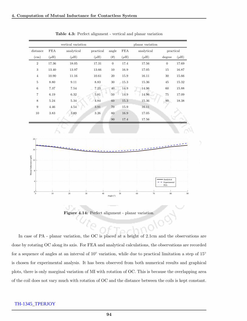
4. Computation of Mutual Inductance for Contactless System
Table 4.3: Perfect alignment - vertical and planar variation
vertical variation planar variation
distance FEA analytical practical angle FEA analytical practical
(cm) (µH) (µH) (µH) (θ) (µH) (µH) degree (µH)
2 17.36 18.05 17.31 0 17.4 17.56 0 17.69
3 13.40 13.97 13.66 10 16.9 17.05 15 16.87
4 10.90 11.16 10.61 20 15.9 16.11 30 15.66
5 8.80 9.11 8.83 30 15.3 15.36 45 15.32
6 7.37 7.54 7.23 40 14.9 14.96 60 15.88
7 6.19 6.32 5.81 50 14.9 14.96 75 17.09
8 5.24 5.34 4.84 60 15.3 15.36 90 18.38
9 4.46 4.54 3.91 70 15.9 16.11
10 3.83 3.89 3.26 80 16.9 17.05
90 17.4 17.56
0 10 20 30 40 50 60 70 80 900
4
8
12
16
20
Angle (°)
Mut
ual I
nduc
tanc
e (µH
)
AnalyticalExperimental
FEA
Figure 4.14: Perfect alignment - planar variation.
In case of PA - planar variation, the OC is placed at a height of 2.1cm and the observations are
done by rotating OC along its axis. For FEA and analytical calculations, the observations are recorded
for a sequence of angles at an interval of 10 variation, while due to practical limitation a step of 15
is chosen for experimental analysis. It has been observed from both numerical results and graphical
plots, there is only marginal variation of MI with rotation of OC. This is because the overlapping area
of the coil does not vary much with rotation of OC and the distance between the coils is kept constant.
94
TH-1345_TPERJOY

4.6 Numerical results and discussion
4.6.2 Lateral misalignment - horizontal and planar variation
In this part, the numerical results for laterally misaligned case of horizontal and planar variation
for all three analysis are summarized and compared. Table 4.4 shows the numerical results of both
horizontal and planar variations. Figure 4.15 and Figure 4.16 shows the corresponding graphical plots.
0 2 4 6 8 100
4
8
12
16
20
Horizontal distance (cm)
Mut
ual i
nduc
tanc
e (µH
)
AnalyticalExperimental
FEA
Figure 4.15: Lateral misalignment - horizontal variation.
In case of LM - horizontal variation, numerical results are obtained for every 1cm distance between
OC and EC horizontally. The MI values are high for initial distance and rapidly decreases when OC
is moved away horizontally from EC.
Table 4.4: Lateral misalignment - horizontal and planar variation
horizontal variation planar variation
distance FEA analytical practical angle FEA analytical practical
(cm) (µH) (µH) (µH) (θ) (µH) (µH) degree (µH)
0 17.39 17.56 18.00 0 11.34 11.35 0 11.43
1 16.94 17.04 16.91 10 11.27 11.29 15 11.57
2 15.65 15.76 15.72 20 11.12 11.14 30 11.22
3 14.30 14.24 14.24 30 11.02 11.02 45 11.09
4 12.70 12.75 12.76 40 10.95 10.96 60 11.19
5 11.31 11.35 11.49 50 10.95 10.96 75 11.53
6 9.98 10.04 10.10 60 11.02 11.02 90 11.50
7 8.74 8.88 8.95 70 11.12 11.14
8 7.54 7.61 7.85 80 11.27 11.29
9 6.48 6.79 6.78 90 11.34 11.35
10 5.47 5.27 5.46
95
TH-1345_TPERJOY

4. Computation of Mutual Inductance for Contactless System
0 10 20 30 40 50 60 70 80 900
5
10
15
Angle (°)
Mut
ual I
nduc
tanc
e (µH
)
AnalyticalExperimentalFEA
Figure 4.16: Lateral misalignment - planar variation.
In case of LM - planar variation, the OC is placed at a height of 2.1cm and fixed at a horizontal
distance of 5cm. The observations are done from the displaced point by rotating OC along its axis.
It has been observed from the results, there is only marginal variation of MI with rotation of OC.
However, the magnitude of MI values got decreased from the PA - planar case. This is because the
overlapping area in the former case is more than the later. Additionally, it can also be inferred from
the results for larger horizontal distance, MI values would have further decreased.
4.6.3 Angular misalignment
In this part, the numerical results for angular misalignment for all three analysis are summarized
and compared. Table 4.5 shows the numerical result of angular misalignment. Figure 4.17 shows the
corresponding graphical plot.
96
TH-1345_TPERJOY

4.6 Numerical results and discussion
0 10 20 30 40 50 60 70 80 900
1
2
3
4
Angle (°)
Mut
ual I
nduc
tanc
e (µH
)
AnalyticalExperimentalFEA
Figure 4.17: Angular misalignment - angular variation.
In case of angular misalignment, OC is placed in a rod of 0.60cm diameter and 12.8cm vertical
height. Numerical values are noted by varying OC along with the rod for angles between 0 to 90.
The variation in MI is found to be marginal due to less change in overlapping area from 0 to 60. As
OC goes beyond 60, it comes almost perpendicular to EC and due to this overlapping area decreases
and MI value falls down drastically.
Table 4.5: Angular misalignment
distance (cm) FEA analytical practical
(θ) (µH) (µH) degree (µH)
0 2.59 2.59 0 2.30
10 2.62 2.62 10 2.35
20 2.69 2.69 30 2.49
30 2.80 2.80 45 2.73
40 2.93 2.94 50 2.73
50 3.05 3.05 70 2.53
60 3.00 3.00 90 1.06
70 2.59 2.59
80 1.79 1.79
90 0.70 0.72
4.6.4 Both lateral and angular misalignment
In this part, the numerical results for a general case of both lateral and angular misalignment for
all three analysis are summarized and compared. The variation in this case is observed by keeping
97
TH-1345_TPERJOY

4. Computation of Mutual Inductance for Contactless System
constant angle and moved horizontally. Thus, three different angles (10, 20 and 30) are chosen and
its variations are observed. Table 4.6 and Table 4.7 shows the numerical results of both lateral and
angular misalignment. Figure 4.18 shows the corresponding graphical plots.
0 2 4 6 8 100
5
10
15
Horizontal distance (cm)
Mut
ual I
nduc
tanc
e (µH
)
10°
20°
30°
AnalyticalExperimentalFEA
Figure 4.18: Both lateral and angular misalignment (angle = 10, 20, 30).
The magnitude of MI value is more for 10 angle and with increase in angle, MI value decreases.
However, MI value falls sharply when OC is horizontally moved away from EC.
Table 4.6: Both lateral and angular misalignment (angle = 10 and 20
angle 10 angle 20
distance FEA analytical practical distance FEA analytical practical
(cm) (µH) (µH) (µH) (cm) (µH) (µH) (µH)
0 11.56 11.47 11.02 0 8.13 8.27 8.25
1.2 11.40 11.27 10.69 1.6 7.98 7.98 8.17
2.2 10.73 10.62 10.29 2.6 7.51 7.50 7.85
3.2 9.81 9.81 9.66 3.6 6.94 6.94 7.36
4.2 9.07 8.94 8.96 4.6 6.35 6.36 6.87
5.2 8.20 8.09 8.17 5.6 5.76 5.76 6.25
6.2 7.34 7.24 7.35 6.6 5.17 5.17 5.63
7.2 6.44 6.41 6.50 7.6 4.56 4.56 5.01
8.2 5.63 5.57 5.72 8.6 3.94 3.92 4.40
9.2 4.75 4.72 4.87 9.6 3.29 3.28 3.68
10.2 3.91 3.85 3.99 10.6 2.62 2.60 3.01
98
TH-1345_TPERJOY

4.7 Conclusions
Table 4.7: Both lateral and angular misalignment (angle = 30)
distance FEA analytical practical
(cm) (µH) (µH) (µH)
0 6.51 6.71 6.53
3.4 5.71 5.70 5.96
4.4 5.23 5.23 5.60
5.4 4.75 4.75 5.18
6.4 4.26 4.26 4.69
7.4 3.78 3.79 4.17
8.4 3.28 3.28 3.08
9.4 2.75 2.75 2.58
10.4 2.19 2.19 1.96
11.4 1.59 1.59 1.37
It has been noticed from the Figure 4.13 - Figure 4.18, the value computed in all the three cases are
in good agreement. However, in some cases there is a slight difference in values between experimental
and calculated (analytical and FEA) results. This is due to the error in measuring the geometrical
parameters such as vertical height, horizontal distance and rotational angle. As an example of a case
of both lateral and angular variation, where the coil has 10 angle shift at 1.2cm distance, MI value
obtained is 12.18µH and at 11 angle it has a value of 11.26µH. Thus, there is 7.5% error occurred
due to error of 1 in angle measurement.
4.7 Conclusions
In this chapter, an analytical method based on Biot-Savart law has been presented for estimating
the MI between two air core square coils. A spiral square coil is modeled and MI is calculated.
Different misalignment cases of contactless and its variations are analyzed. The analysis compares the
analytical, FEA and experimental results in all misalignment cases. The analytical and FEA results
show a very good agreement and experimental results has an error less than 10%. The following
conclusions are drawn from the work:
• When the coils are placed close to each other with coinciding axes, MI values are maximum;
which indicates high coupling between the coils and expected to have maximum power transfer
in CPT systems.
• At large coil distances, relatively large horizontal and vertical misalignments; MI have no sig-
99
TH-1345_TPERJOY

4. Computation of Mutual Inductance for Contactless System
nificant effects. This indicates relatively low coupling in CPT system and it would not transfer
any power.
• In case of planar variation MI value would vary marginally. Such type of variation would not
affect the power transfer in CPT systems.
• An interesting behavior of MI is observed in angular misalignment, tilting OC at certain angle
brings half of the coil closer to the perimeter of EC and due to this MI value increases and for
other angles, MI values would suddenly decrease. Such type of variations in practical systems
would cause instability.
From the results it has been noticed; larger the distance between EC and OC, lowers the coupling
coefficient and MI value. This is due to large leakage inductance and reduced magnetizing inductance.
Hence, compensation elements can be used on both sides of contactless coils to improve the MI value
and to increase the power transfer capability. The next chapter has analyzed the use of four such
compensation topologies in contactless system.
100
TH-1345_TPERJOY

5Compensation Topologies for
Contactless System
Contents
5.1 Introduction . . . . . . . . . . . . . . . . . . . . . . . . . . . . . . . . . . . . 103
5.2 Steady state electric circuit analysis . . . . . . . . . . . . . . . . . . . . . . 106
5.3 Description of experimental set-up . . . . . . . . . . . . . . . . . . . . . . . 117
5.4 Results and discussion . . . . . . . . . . . . . . . . . . . . . . . . . . . . . . 124
5.5 Conclusions . . . . . . . . . . . . . . . . . . . . . . . . . . . . . . . . . . . . 137
101
TH-1345_TPERJOY

5. Compensation Topologies for Contactless System
102
TH-1345_TPERJOY

5.1 Introduction
Abstract
Due to large leakage inductance, compensations circuits are necessary in contactless system to achieve
the required power transfer. This chapter presents an experimental study of four compensation topolo-
gies connected on both sides of coils suitable for use in contactless charging system applications.
Primary compensation is designed to make the primary phase angle equal to the secondary reso-
nant frequency with minimum VA rating of the power supply. Secondary compensation is designed
to increase the power transfer capability. Equivalent circuit models are used to explain the theory
of contactless system with analytical expressions for voltage, current and impedance as well as the
power transfer efficiency, by combining the primary and secondary network is detailed. The study
investigates the behavior of compensation circuits in contactless system under variable frequency, load
and distance and its characteristics plots are generated. The analysis compares the efficiency of four
compensation topologies such that the real time performance of CPT systems can be analyzed. With
these results obtained from the experiments, the theory of CPT systems can be well understood and
it provides a foundation for future design and implementation of CPT systems.
The work presented in this chapter is accepted for publication in [133, 134] and sub-
mitted in [135, 136].
5.1 Introduction
The energy supply in electrical system is commonly realized by conventional plug and socket
connectors and the power transfer equipment is one of the important subsystems. The traditional
conductive wired systems cannot keep up with the present demands of customers in safety and sim-
plicity [137]. With the developments in power electronics, CPT system has found much success due
to its simplicity, size and reliability [29], which has been explained in chapter I. The principle of CPT
system is similar to a conventional transformer, where the magnetic field is confined to a particular
core. In contrast to conventional transformer, contactless transformer has a large air-gap and are used
without high permeability common magnetic core [31]. This technology utilizes magnetic filed around
a current carrying wire to magnetically couple power across large air-gap through weak magnetic cou-
pling. Due to this large air-gap, the characteristics of contactless system has large leakage inductance
and reduced magnetizing inductance and low efficiency as compared to conductive wired systems. To
103
TH-1345_TPERJOY

5. Compensation Topologies for Contactless System
compensate large leakage inductance problem effectively, suitable compensation circuit can be added
by connecting a series or parallel capacitor at the primary and secondary winding of the coil as shown
in Figure 5.1 [71]. This makes the contactless circuit to operate at resonance and achieves maximum
output power with minimum input VA rating of the power supply.
supply
Power
converter
frequency
High Primary
compensation
Primary
winding
Secondary
winding
Secondary
compensationRectifierLoad
Contactless coil
Magnetic
coupling
Figure 5.1: Block diagram of contactless system with compensation.
In addition, there could be an application where the system is connected to the variable load and
the secondary side of the coil must be moved with the primary coil [32, 36, 37]. In such cases, the
leakage inductance of the coils are larger than the magnetizing inductance leading to inefficient power
transmission. CPT systems basically has a high frequency power converter to feed the coil at the
input side and a rectifier in the secondary side connected to the load. The specifications of converter,
controllers and its parameters differs for each applications. The frequency of the power supply should
be controlled to attain a zero phase angle between the voltage and current at the input side of the
coil [35]. Therefore, the role of compensations circuits in CPT systems and its impact for variations
in parameters must be studied which is the first step in the design of such systems.
There are many applications of CPT systems exists in the literature. Power conversion methods
and controllers of CPT system are reported in [29,107,109,138–140], while other researches have worked
on the design of magnetic coupling structures [137,141]. Many other works have paid attention on the
design of contactless coil [23,45]. A very few works have studied compensation circuits in contactless
system. Optimized design procedures are given to select the suitable compensation topology for
efficient power transfer [23, 31, 36, 45]. In [34, 35, 142, 143], CPT model is analyzed to investigate
104
TH-1345_TPERJOY

5.1 Introduction
the sensitivity of the system for variation in operational frequency and load. In [22] and [143], an
occurrence of bifurcation due to multiple operating modes in CPT system have been studied using
higher order mathematical models. Few other works have studied the power transfer capability of
contactless systems using compensation circuits [144, 145]. However, a very few works have studied
the impact of system parameters in CPT systems. Among those, the most critical parameters are
frequency, load, low magnetizing inductance and high leakage inductance. It has been found, there are
no experimental investigation done so far to analyze the power transfer capability and controllability
of the system. In this chapter, an experimental investigation have been done with four compensation
!!
!!
b1
a1
a2
b2
M
h
Figure 5.2: Coil topology.
topologies using rectangular primary (18cm × 14.5cm) and secondary coil (19cm × 11cm) shown in
Figure 5.2. The primary side and secondary side of the coil is examined with both series and parallel
compensation circuits. Series compensated primary is chosen to reduce the primary voltage level, while
a parallel compensated secondary is able to supply a stable current. A series compensated secondary
can supply a stable voltage, while a parallel compensated secondary is able to supply a stable current.
Of particular interest, this work has studied the impact of compensation circuits for variation in
frequency, distance and load; so that the practical behavior of CPT system can be visualized. The
105
TH-1345_TPERJOY

5. Compensation Topologies for Contactless System
analysis have been carried out by fixing the number of turns in primary and secondary side. Other
prefixed parameters in this study are coil shape, dimensions of the coil and circuit topology. The
variable parameters are air gap distance, operating frequency and load. Skin effect is not considered
because both coils are wound using multi-strand copper wire. Electric equivalent circuit models of
different compensation topologies are developed to explain the mechanism of power transfer. The
performance of four compensation topologies are validated and its results are analyzed. The analysis
compares the efficiency of four basic topologies of CPT system with variation in frequency, distance
and load.
The rest of the chapter is organized as follows: Section 5.2 describes the steady state electric circuit
analysis. Section 5.3 presents the description of experimental set-up. Finally, experimental results are
presented in Section 5.4 and its conclusions are given in Section 5.5.
5.2 Steady state electric circuit analysis
For the purpose of mathematical analysis, the steady state behavior of air core transformer with a
large air gap can be described by an equivalent circuit. An electric equivalent circuit makes the process
of network analysis easier. CPT system combines two coupled primary and secondary windings, similar
to a conventional transformer. Unlike transformer windings, contactless systems are usually loosely
coupled without any common magnetic core. Hence, contactless system has large leakage inductance
and therefore, compensations are required on both sides of the coils.
5.2.1 Compensation topologies
The purpose of compensation capacitors in contactless system is to increase its efficiency. Com-
pensation capacitors are connected on both sides of primary and secondary windings of contactless
coils. The purpose of primary compensation is to decrease the VA rating of the power supply and
thereby ensuring power transfer at unity power factor and the purpose of secondary compensation is to
enhance the power transfer capability. The primary compensation is chosen such that the impedance
as seen from the source side is purely resistive in nature so as to ensure that the high frequency inverter
which acts as the primary power source has minimum possible VA rating of the power supply. Four
such compensation topologies are described in this chapter. Four compensation topologies are repre-
sented as SS, SP, PS and PP topology as shown in Figure 5.3, where ‘S’ stands for series connected
topology and ‘P’ stands for parallel connected topology. Hence, series-series is named as SS topology,
106
TH-1345_TPERJOY

5.2 Steady state electric circuit analysis
series-parallel as SP topology, parallel-series as PS topology and parallel-parallel as PP topology. In
Figure 5.3, I1, IL1, IC1 denotes supply current, inductor current and capacitor current of the primary
side and IL2, IC2 and IL represents inductor current, capacitor current and load current of secondary
side respectively. Similarly, L1, C1 and V1 denotes inductor, capacitor and supply voltage in the pri-
mary side and L2, C2 and RL denotes inductor, capacitor and load resistance in the secondary side
respectively. The main criteria to increase the power transfer capability in all compensation is that
RL
C1
V1
C2I1 IC1
ILIL1
M
L2
IC2
L1
IL2
(a)
RL
C1
V1
IC1
M
C2
L1 L2
ILIL1 IL2 IC2
I1
(b)
RL
V1
IL
M
IC1
C1
C2
IC2IL1 IL2
L1 L2
I1
(c)
RL
V1
ILIL1 IL2
M
IC1
C1 C2
IC2
L1 L2
I1
(d)
Figure 5.3: Equivalent circuit model of contactless coils (a) SS topology (b) SP topology (c) PS topology (d)PP topology.
the primary side of the system should operate at secondary side resonance frequency. When operating
at secondary resonance frequency, the self inductance of the secondary winding is fully compensated
by the primary compensation capacitance. Therefore, the impedance of the secondary as seen by
the primary is purely resistive in nature. Thus, these capacitors essentially store and supply reactive
power to and from the secondary and primary windings, reducing the amount of reactive power drawn
from the supply.
5.2.2 Mutual inductance coupling model
The coupling between the primary and secondary coil and its operation can be analyzed using
several modeling methods. Among various modeling methodologies, transformer model and mutual
inductance coupling model are the most commonly used methods. The transformer model uses the
concept of transformed voltage and reflected current to describe the coupling effects. The transformed
voltage and reflected currents are simply defined by the turns ratio. Here, the coupling and leakage
107
TH-1345_TPERJOY

5. Compensation Topologies for Contactless System
inductance must be separated by circuit analysis. This coupling model is well suited for closely coupled
CPT systems because the leakage inductance is usually negligible. In contrast, mutual inductance
coupling model uses the concept of induced and reflected voltages to describe the coupling effect
between the primary and secondary networks. Both the induced and reflected voltages are expressed
in terms of the mutual inductance. This model does not require the coupling and leakage inductance
to be separated for circuit analysis. Hence this model is well-suited for loosely coupled CPT systems,
where the leakage inductance is too large to be ignored. In this chapter, mutual inductance model is
used to analyze the coupling between the primary and secondary coils of CPT systems. The effect of
the secondary must be considered together with the primary winding in the analysis of the primary
network. Therefore, the effect of secondary can be represented by the equivalent reflected impedance.
Compensation elements are required to compensate leakage inductance of the coil. The compensation
elements can be connected in series or parallel on primary and secondary sides of the coil. For
simplification purpose, neglecting coil resistances, the analysis of four compensation topologies using
mutual inductance coupling models are presented in the following section.
5.2.3 Series-series (SS) compensation topology
Assuming all currents are sinusoidal, the steady state equations for primary and secondary series
compensation can be written on phasor form as given by (5.1) and (5.2)
V1 = I1
(1
jωC1
)+ jωL1I1 − jωMI2 (5.1)
jωMI1 = jωL2I2 + I2
(1
jωC2
)+ I2RL (5.2)
where mutual inductance of the coil (M) is given by (5.3). From (5.1)-(5.2) it is observed, both the
induced voltage and reflected voltage are represented in terms of mutual inductance (M) between
the coils to describe the coupling effect between the primary and secondary network. The mutual
inductance can be related with the magnetic coupling (k) as given by (5.3).
k =M√L1L2
(5.3)
The magnetic coupling of contactless coil is usually poor. In (5.3), the coupling between the primary
and secondary of the coil depends on the leakage inductance (L1, L2) and magnetizing inductance
(M). The leakage inductance in contactless coil is much larger than the magnetizing inductance. On
108
TH-1345_TPERJOY

5.2 Steady state electric circuit analysis
simplifying (5.2), current I2 in series secondary coil can be written as (5.4).
I2 =jωMI1[
jωL2 +(
1jωC2
)+RL
] (5.4)
On substituting secondary side current I2, given in (5.4) into (5.1), we get:
V1 = I1
(1
jωC1
)+ jωL1I1 +
ω2M2
jωL2 +(
1jωC2
)+RL
I1 (5.5)
It can be observed from (5.5), from the point of view of the first coil, the secondary coil is seen as a
transformed impedance or reflected impedance (Zr) of the secondary network as seen from the primary
side. Hence, for series compensated secondary:
Zr SS =ω2M2
[jωL2 +
(1
jωC2
)+RL
] =ω2M2
Z2S
(5.6)
where, ZsS is the secondary side impedance. The total impedance (Zt) for series and parallel com-
pensated system seen by the power supply is obtained from (5.5) is given by (5.7).
Zt SS =
(1
jωC1
)+ jωL1 +
ω2M2
jωL2 +(
1jωC2
)+RL
(5.7)
Now the simplified version of contactless system is shown in Figure 5.4(a) and Figure 5.4(b) Therefore,
V1
Zr
C1I1
L1
(a)
I1
V1Zt
(b)
Figure 5.4: Simplified equivalent circuit (a) with reflected impedance (b) with total impedance.
the current observed from the source is given by (5.8).
I1 =V1
Zt SS(5.8)
109
TH-1345_TPERJOY

5. Compensation Topologies for Contactless System
In order to obtain high power transfer capability, the operating frequency of the system should be
equal to the secondary resonant frequency (ωo), which is given by (5.9)
ωo =1√L2C2
(5.9)
On substituting (5.9) into (5.6), we get the reflected impedance as given by (5.10).
Zr SS =ωo
2M2
RL=ω2
oM2
ZsS
(5.10)
It can be observed from (5.10), if the secondary is series compensated Zr SS is purely resistive. Thus
to obtain high efficiency, the primary side of the system should operate at resonance frequency of the
secondary side of the system. Therefore for SS compensation, C1 and C2 can be given by (5.11).
C1 =1
ωo2L1
; C2 =1
ωo2L2
(5.11)
Then, the total impedance of the system is given by (5.12).
Zt SS =ωo
2M2
RL(5.12)
On substituting (5.11) into (5.2), the relation between I2 and I1 can be obtained, where I2 leads I1
at some angle.
I2I1
=jωoM
RL
(5.13)
I2 = G1I1 ; G1 =jωoM
RL(5.14)
Using (5.1) - (5.14), the input power (Pi), output power (Po) and total efficiency of the system are
calculated.
Pi = I12Zt SS (5.15)
Po = I22RL = G2
1I21RL (5.16)
Using these equations, efficiency for SS compensation is given by (5.17).
ηSS =G2
1RL
Zt SS
(5.17)
110
TH-1345_TPERJOY

5.2 Steady state electric circuit analysis
5.2.4 Series-parallel (SP) compensation topology
The steady state equations for primary series and secondary parallel compensation can be written
on phasor form as given by (5.18) and (5.19)
V1 = I1
(1
jωC1
)+ jωL1I1 − jωMI2 (5.18)
jωMI1 = jωL2I2 + I2
RL
(1
jωC2
)
RL +(
1jωC2
)
(5.19)
Similar to the procedure explained in Section 5.2.3, simplifying (5.19), current I2 in parallel secondary
coil can be written as (5.20).
I2 =jωMI1[
jωL2 +
(RL
(1
jωC2
)
RL+(
1jωC2
)
)] (5.20)
By substituting secondary side current I2, given in (5.20) into (5.18), we get
V1 = I1
(1
jωC1
)+ jωL1I1 +
ω2M2
jωL2 +(
RL
RLjωC2+1
)
I1 (5.21)
It can be observed from (5.21), from the point of view of the first coil, the secondary side parallel
compensated coil is seen as a transformed impedance or reflected impedance (Zr SP ) of the secondary
network as seen from the primary side. Therefore, Zr SP and Zt SP is given by (5.22) and (5.23).
Zr SP =ω2M2
[jωL2 + RL
RLjωC2+1
] =ω2M2
Z2P
(5.22)
Zt SP =1
jωC1+ jωL1 +
ω2M2
jωL2 +(
RL
jωC2RL+1
) (5.23)
The current observed from the source is given by (5.24)
I1 SP =V1
Zt SP(5.24)
In order to obtain high power transfer capability, the operating frequency of the power supply should
be equal to the secondary resonant frequency (ωo) and the secondary side compensation capacitor C2
is given by (5.25)
C2 =1
ωo2L2
(5.25)
111
TH-1345_TPERJOY

5. Compensation Topologies for Contactless System
When operating the CPT system at this frequency, the self inductance of the secondary winding is fully
compensated by the primary compensation capacitor and therefore the impedance of the secondary
as seen by the primary is purely resistive in nature. Therefore, on substituting (5.25) into (5.22) and
(5.23), the secondary side impedance (Z2P ) and the reflected impedance (Zr SP ) is given by (5.26)
and (5.27).
Z2P =
ωo2L2
2
RL − jωoL2(5.26)
Zr SP =M2RL
L22 − jωoM
2
L2(5.27)
It can be observed from (5.27), if the secondary is parallel compensated it has a reactive component.
This introduces a phase shift in the system. This phase shift (−M2
L2) should be compensated in the
primary side of the system. For this reason, a large primary capacitance is usually used in parallel
compensated CPT system. Therefore, in order to operate the SP compensated CPT system under
resonance frequency and to obtain high efficiency, the compensated capacitors, C1 and C2 are given
by (5.28).
C1 =1
ωo2(L1 − M2
L2
) ; C2 =1
ωo2L2
(5.28)
The total impedance (Zt SP ) at resonance is given by (5.29)
Zt SP =M2RL
L22 (5.29)
On substituting (5.28) into (5.19), the relation between I2 and I1 can be obtained, where I2 leads I1
at some angle.
I2I1
=jωM(ωo
2L22
RL−jωoL2
) (5.30)
I2 = G2I1 =jωoM (RL − jωoL2)
ωo2L2
2 (5.31)
Using (5.18) - (5.31), the input power (Pi), output power (Po) and total efficiency of the system are
calculated.
Pi = I12Zt SP (5.32)
Po = I22RL = G2
2I21RL (5.33)
Using these equations, efficiency for SP compensation is given by (5.34).
ηSP =G2
2ωo2L2
2
Zt SP (RL − jωoL2)(5.34)
112
TH-1345_TPERJOY

5.2 Steady state electric circuit analysis
5.2.5 Parallel-series (PS) compensation topology
The steady state equations for primary parallel and secondary series compensation can be written
on phasor form as given by (5.35) and (5.36)
V1 = IC1
(1
jωC1
)= IL1jωL1 − jωMI2 (5.35)
jωMIL1 = jωL2I2 + I2
(1
jωC2
)+ I2RL (5.36)
The secondary side current I2 in PS compensation can be obtained from (5.37).
I2 =jωMIL1
jωL2 +(
1jωC2
)+RL
(5.37)
By substituting the secondary side current I2, given in (5.37) into (5.35), we get
V1 = jωL1IL1 +ω2M2
jωL2 +(
1jωC2
)+RL
IL1 (5.38)
As explained above, from the point of view of the first coil, the secondary coil is seen as a transformed
impedance or reflected impedance (Zr PS) of the secondary network as seen from the primary side is
given by (5.39).
Zr PS =ω2M2
[jωL2 + 1
jωC2+RL
] =ω2M2
Z2s (5.39)
On substituting (5.37) in (5.35), the current through primary side inductor (IL1) and capacitor (IC1)
is obtained.
IL1 =V1
jωL1 + ω2M2
Z2s
(5.40)
IC1 =V11
jωC1
(5.41)
From Figure 5.5, the total impedance (Zt PS) of the PS compensation is given by (5.42). The total
V1C1
I1
Zr PS
IC1 IL1
L1
Figure 5.5: Parallel compensated primary.
113
TH-1345_TPERJOY

5. Compensation Topologies for Contactless System
current observed from the primary side is given by (5.43).
Zt PS =1
jωC1 + 1jωL1+Zr PS
(5.42)
I1 PS =V1
Zt PS
(5.43)
To obtain high efficiency in PS compensated CPT system, the system should operate under resonance
condition. The resonance capacitance for parallel and series compensated primary is same as the basic
resonance condition as given by (5.44).
C1 =1
ωo2L1
(5.44)
On substituting (5.44) into (5.42), the total impedance at resonance condition is given by
Zt PS =Z2
SL12
M2− jωoL1 (5.45)
It has been seen from (5.45) has some constraints on (Z2S) for the system to be in resonance. While
for the system to be in parallel compensated, Z2S has some resistive and reactive part, say
Z2S = RL + jX (5.46)
The criteria for resonance is, the inductance due to parallel primary side should be compensated in
the secondary side coil such that the primary side impedance is resistive in nature. This condition is
achieved when the reactance is in the form given below:
X = ωoM2
L1(5.47)
On substituting (5.46) in (5.42) and (Zt PS) can be obtained as given by (5.48)
Zt PS =RLL1
2
M2(5.48)
Thus, when the primary side is parallel compensated a phase shift is introduced to the secondary side
that brings the secondary side out of resonance. Therefore, the compensation capacitance in PS is
defined as given below:
C1 =1
ωo2L1
; C2 =1
ωo2(L2 − M2
L1
) (5.49)
114
TH-1345_TPERJOY

5.2 Steady state electric circuit analysis
Using these condition (5.49), the secondary side impedance (Z2S) given in (5.39) can be given by
(5.50).
Z2S = jωo
M2
L1+RL (5.50)
The secondary current (I2) can be given in (5.36) can be modified by substituting IL1 and Z2S given in
(5.50) and (5.40). Therefore, I2 at resonance can be written as given by (5.51). The primary current
(I1) can be written as given by (5.52).
I2 =M
L1RLV1 (5.51)
I1 =M2
RLL12V1 (5.52)
Using (5.37) and (5.52), the input power (Pi), output power (Po) and total efficiency of the system
are calculated.
5.2.6 Parallel-parallel (PP) compensation topology
The steady state equations for primary and secondary parallel compensation can be written on
phasor form as given by (5.53) and (5.54)
V1 = IC1
(1
jωC1
)= IL1jωL1 − jωMI2 (5.53)
jωMIL1 = jωL2I2 + I2
11(1
jωC2
) + 1RL
(5.54)
The secondary side current I2 in PP compensation can be obtained from (5.55).
I2 =jωM(
jωL2 + RL
RLjωC2+1
)IL1 =jωM
Z2p IL1 (5.55)
By substituting the secondary side current I2 (given in (5.55)) into (5.53) we get:
V1 = jωL1IL1 +
(ω2M2
jωL2 + RL
RLjωC2+1
)IL1 (5.56)
As explained above, from the point of view of the first coil, the secondary coil is seen as a transformed
impedance or reflected impedance (Zr PP ) of the secondary network as seen from the primary side
and is given by (5.57).
Zr PP =ω2M2
jωL2 + RL
jωC2RL+1
=ω2M2
Z2p (5.57)
115
TH-1345_TPERJOY

5. Compensation Topologies for Contactless System
From (5.56), the current through primary side inductor (IL1) and capacitor (IC1) is obtained. The
total impedance (Zt PP ) of PP compensation is given by (5.60).
IL1 =V1
jωL1 + ω2M2
Z2p
(5.58)
IC1 =V11
jωC1
(5.59)
Zt PP =1
1
jωL1+ω2M2
Z2P
+ jωC1(5.60)
The total current observed from the primary side is given by (5.61).
I1 =V1
Zt PP(5.61)
In case of parallel compensated primary and secondary, the system has reactive components, which
introduces phase shifts on both sides of the system (as explained above). Hence for parallel compen-
sated system, the compensation capacitors are defined as given by (5.62). This is the reason a large
primary and secondary capacitor is usually added on both sides of CPT systems.
C1 =1
ωo2(L1 − M2
L2
) ; C2 =1
ωo2(L2 − M2
L1
) (5.62)
On substituting (5.61), the secondary side impedance (Z2S), reflected impedance (Zr PP ) and total
impedance (Zt PP ) can be derived as given by (5.63)-(5.65).
Z2p =
ωo2L2
(L2 − M2
L1
)+ jωo
M2
L1RL
RL − jωo
(L2 − M2
L1
) (5.63)
Zr PP =ω2M2
(RL − jωo
(L2 − M2
L1
))
ωo2L2
(L2 − M2
L1
)+ jωo
M2
L1RL
(5.64)
Zt PP =ωo
2L12 − ωo
2L1M2
L2− jωoL1Zr PP + jωo
M2
L2Zr PP
jωoM2
L2+ Zr PP
(5.65)
The primary current and load current is given by (5.66) and (5.67).
I1 =V1
Zt PP
=jωo
M2
L2+ Zr
ωo2L1
2 − ωo2L1
M2
L2− jωoL1Zr + jωo
M2
L2Zr
V1 (5.66)
IL =VL
RL
=ZpI2RL
=I2
(RLjωC2 + 1)(5.67)
116
TH-1345_TPERJOY
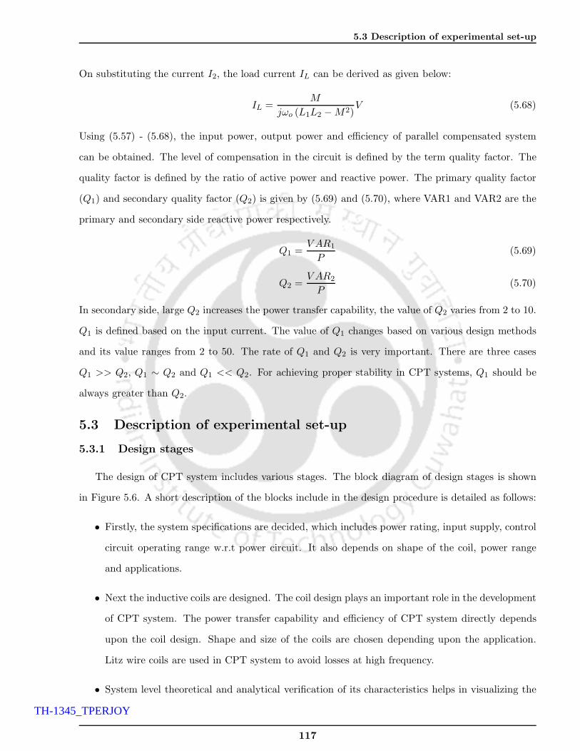
5.3 Description of experimental set-up
On substituting the current I2, the load current IL can be derived as given below:
IL =M
jωo (L1L2 −M2)V (5.68)
Using (5.57) - (5.68), the input power, output power and efficiency of parallel compensated system
can be obtained. The level of compensation in the circuit is defined by the term quality factor. The
quality factor is defined by the ratio of active power and reactive power. The primary quality factor
(Q1) and secondary quality factor (Q2) is given by (5.69) and (5.70), where VAR1 and VAR2 are the
primary and secondary side reactive power respectively.
Q1 =V AR1
P(5.69)
Q2 =V AR2
P(5.70)
In secondary side, large Q2 increases the power transfer capability, the value of Q2 varies from 2 to 10.
Q1 is defined based on the input current. The value of Q1 changes based on various design methods
and its value ranges from 2 to 50. The rate of Q1 and Q2 is very important. There are three cases
Q1 >> Q2, Q1 ∼ Q2 and Q1 << Q2. For achieving proper stability in CPT systems, Q1 should be
always greater than Q2.
5.3 Description of experimental set-up
5.3.1 Design stages
The design of CPT system includes various stages. The block diagram of design stages is shown
in Figure 5.6. A short description of the blocks include in the design procedure is detailed as follows:
• Firstly, the system specifications are decided, which includes power rating, input supply, control
circuit operating range w.r.t power circuit. It also depends on shape of the coil, power range
and applications.
• Next the inductive coils are designed. The coil design plays an important role in the development
of CPT system. The power transfer capability and efficiency of CPT system directly depends
upon the coil design. Shape and size of the coils are chosen depending upon the application.
Litz wire coils are used in CPT system to avoid losses at high frequency.
• System level theoretical and analytical verification of its characteristics helps in visualizing the
117
TH-1345_TPERJOY

5. Compensation Topologies for Contactless System
Power converter and driver circuit design
Compensation design
Hardware development
Check the final circuit
Specification of CPT system
Selection of coil topology, coil desigm
System level theoretical analysis
Figure 5.6: Block diagram of design procedure.
behavior of CPT system.
• Following to which, the power converter and driving circuit design can be done.
• The choice of primary and secondary compensation topology is also an important stage in the
design of CPT system. By which, the load connected to the CPT system is seen as an ohmic
load from the power supply side. The compensation topology determines the system behavior
and sensitivity for variable load and air gap distance.
• Finally the development, building and testing of CPT system prototype is done.
5.3.2 Block diagram
The CPT system can be controlled with either fixed frequency control or variable frequency control.
In the first case, the system is controlled to supply the load with fixed voltage and frequency. While
118
TH-1345_TPERJOY

5.3 Description of experimental set-up
in the second case, the system is controlled to supply the load with variable voltage and frequency. In
this work, PWM based variable frequency control has been used to control the power converter of the
CPT system. The basic building blocks of CPT system is shown in Figure 5.7. The complete layout
converter
full bridge
driver
gate gate
driver
Rectifier Load
PWM
Controller
+8V+8V+15V +15V +8V+Vs
g7
g10
g9
g8
Figure 5.7: Basic building blocks of CPT system.
of CPT system consists of five blocks : full bridge converter, gate driver, PWM controller, rectifier
module and load. As already explained, the primary and secondary side of the system is physically
isolated and magnetically coupled to each other. The primary side of the coil is connected to a full
bridge converter. The full bridge converter is controlled by a PWM based frequency control to control
the power output of the CPT system. To increase the power output and to amplify the gate signal
two gate driver circuits are used to control the high and low side switches. The secondary winding of
the coil is connected to full bridge rectifier block and load.
5.3.3 Power circuit and coil description
The CPT system is built in the laboratory to validate the performance of four compensation
topology. The primary and secondary windings of contactless coils forms a system of magnetically
coupled inductor. The inductive coils are powered by a full bridge converter. The primary winding of
inductive coil is connected through full bridge inverter (S7-S10), while secondary winding is connected
through diode rectifier module (D11-D14) to the load. The primary side full bridge converter con-
sists of MOSFET based inverter and converts rectified dc link voltage into alternating voltage. This
119
TH-1345_TPERJOY

5. Compensation Topologies for Contactless System
Contactless coilPrimary side − Inverter Secondary side − Rectifier
LsRL
M
Lp
C1 C2
Vdc
S7 S9
S10 S8 D12
D13
D14
D11
Figure 5.8: Power circuit.
alternating voltage supplied in the primary coil generates a magnetic field which induces a current
in the secondary coil. The induced voltage in the secondary side of the coil is rectified using diode
rectifier (D11-D14) shown in Figure 5.8 is connected to the load RL (can be used to power a device
or storage system). Load in the circuit is varied from 1.2Ω to 38Ω. Due to large leakage inductance
of CPT system and to improve the power transfer capability, compensation capacitors (C1, C2) are
used on both sides of the inductive coils (SS compensation is shown in Figure 5.8). The method of
compensation are chosen based on the application of CPT system. Compensation capacitors C1 and
C2 are chosen to be different based on the topology and its design equations are given in Section 5.2.
Different ceramic capacitors ranging from 3.998µF to 8.454µF have been used as compensation capac-
itors in the CPT system. The compensation capacitors along with coil inductor acts as LC filter to
remove the voltage and current ripples in the circuit. The full bridge converter switches in the primary
side are controlled to control the power flow in the system. For this purpose, PWM based frequency
controller is used with two gate driving circuits to drive high and low side MOSFETs. The frequency
of the converter is controlled by a frequency controller which helps to adjust the instantaneous value
of primary peak current and voltage and guarantees the zero phase difference at resonance condition.
The power converter in the primary side is made of high power switching MOSFET IRF540 of 100V,
30A have been used to meet the desired voltage and current requirements for triggering the switches
(S7 - S10) of the converter. The primary and secondary side of inductive coils are made of 10 turns of
multi-strand AWG#25 copper wire. The secondary side diode rectifier is build of QRD0610T30 fast
recovery diode module having reverse blocking voltage of 600V and average forward current of 50A.
120
TH-1345_TPERJOY

5.3 Description of experimental set-up
The inductive coils are wounded on two same sized separate piece of wooden board placed in parallel
using supporting staffs separated by an air gap. The coils are wound in spiral fashion to represent a
closed square and rectangular coil to provide a complete current path. The arrangement is made such
that the primary coil is fixed for all experiments and the secondary coil is varied over 2cm to 10cm
vertical distance. Four wooden staffs are used and the arrangement of the set-up is made in such
a way that the air-gap distance between the coil can be adjusted to observe its variation over large
vertical distance (h) as shown in Figure 5.2. Hence, leakage inductance of the coil may also change in
a wide range.
5.3.4 Control circuit description
The control circuit of CPT system has been designed to perform reliable and stable operation.
Low cost, highly reliable PWM based controller has been used to control the power circuit of CPT
system. The gate pulses (g7- g10) for the converter switches are provided from IR2110 driver circuit.
Two gate drivers provides high and low side outputs (HO and LO), which is given as gate pulses. The
IR2110 is supplied from SG3525 PWM controller. The outputs of PWM controller are HIN and LIN.
The frequency of the controller has been designed to vary from 200Hz and 200kHz. The control circuit
is made to adjust the switching frequency of the converter to operate at variable range of frequencies.
Variable frequency controller have been used because the power supply of the inductive coils have to
be regulated to keep the minimum difference of phase angle between primary voltage and current by
changing its operating frequency at resonance. The control blocks of CPT system can be divided into
two stages. The first stage is pulse width modulation (PWM) based control signal generation stage,
which controls the frequency of the pulses of the converter. The second stage is the driver stage which
obtains input from first stage circuit and amplifies the high and low side gate drive signal for switching
on the MOSFET. The detailed block representation of control circuit is shown in Figure 5.9. In the
first stage, SG3525 based PWM controller have been used to control the frequency of the converter.
The frequency of the PWM controller is dependent on the value of timing capacitor (Ct) and resistor
(Rt), which is externally connected to the circuit. To avoid short circuits in the legs of the converter
dead time have been introduced using a potentiometer (Rd) in the circuit. The output frequency of
the frequency controller (HIN and LIN) is determined using the in-built oscillator present in SG3525
controller, where the frequency of the system is controlled using timing resistor (Rt), timing capacitor
(Ct) and damping resistor (Rd). Here, dead time is provided using Rd to avoid short circuits in the
121
TH-1345_TPERJOY
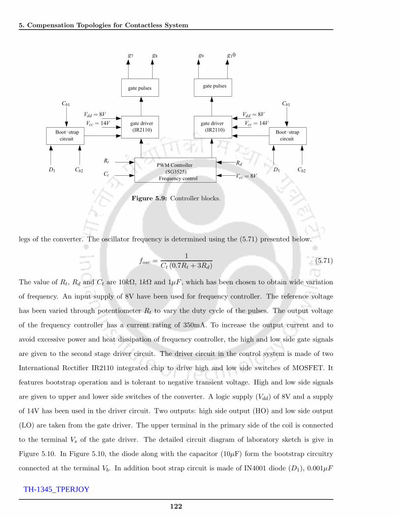
5. Compensation Topologies for Contactless System
Boot−strap
circuit
Boot−strap
circuit
(IR2110) (IR2110)
gate pulses gate pulses
PWM Controller
(SG3525)
Frequency control
gate driver gate driver
D1 D1
Cb1
Cb2
Cb1
Cb2
g7 g8 g9 g10
Vdd = 8V
Vcc = 14V
Rd
Vcc = 8VCt
Rt
Vdd = 8V
Vcc = 14V
Figure 5.9: Controller blocks.
legs of the converter. The oscillator frequency is determined using the (5.71) presented below.
fosc =1
Ct (0.7Rt + 3Rd)(5.71)
The value of Rt, Rd and Ct are 10kΩ, 1kΩ and 1µF , which has been chosen to obtain wide variation
of frequency. An input supply of 8V have been used for frequency controller. The reference voltage
has been varied through potentiometer Rt to vary the duty cycle of the pulses. The output voltage
of the frequency controller has a current rating of 350mA. To increase the output current and to
avoid excessive power and heat dissipation of frequency controller, the high and low side gate signals
are given to the second stage driver circuit. The driver circuit in the control system is made of two
International Rectifier IR2110 integrated chip to drive high and low side switches of MOSFET. It
features bootstrap operation and is tolerant to negative transient voltage. High and low side signals
are given to upper and lower side switches of the converter. A logic supply (Vdd) of 8V and a supply
of 14V has been used in the driver circuit. Two outputs: high side output (HO) and low side output
(LO) are taken from the gate driver. The upper terminal in the primary side of the coil is connected
to the terminal Vs of the gate driver. The detailed circuit diagram of laboratory sketch is give in
Figure 5.10. In Figure 5.10, the diode along with the capacitor (10µF) form the bootstrap circuitry
connected at the terminal Vb. In addition boot strap circuit is made of IN4001 diode (D1), 0.001µF
122
TH-1345_TPERJOY

5.3 Description of experimental set-up
and 0.0001µF capacitor to amplify the signal, then the output gate signal (g7, g8, g9, g10) is supplied
to high and low side switches of the voltage source converter.
1K
1K
1K
1K
+8V +15V
+8V SG3525
+15V +8V
Driver CircuitPower CircuitDriver CircuitPWM Controller
IR2110 IR2110
IRF540IRF540
IRF540
diode moduleQRD0610T30
IRF540
RL
22Ω
22Ω22Ω
22Ω
Vs
10µF
Vcc Vcc
Vs
VB
+Vcc
L1
C2
C1
g1 g3
g4g2L2
Rt Ct
RdLIN HIN
HIN
Vdd HO
LO
S7 S9
HIN
Vb
HO
LINLO
LINS10S8
D11
D12
D13
D14
Vdd
Figure 5.10: Power circuit connected with controller.
The CPT system is designed for a frequency of 15.432kHz. The circuit parameters of the inverter
module are same as shown in Table 5.1. Figure 5.11 shows the view of the experimental prototype
made in the laboratory.
CompesationCapacitor
ContactlessCoils
Rectifier
CompesationCapacitor
FrequencyController
Load
DriverCircuit
Converter
Figure 5.11: Experiential set-up.
123
TH-1345_TPERJOY

5. Compensation Topologies for Contactless System
Table 5.1: Specifications.
Specification Term SS SP PS PP
N1 Number of primary turn 10 10 10 10N2 Number of secondary turn 10 10 10 10L1 Primary side inductance 26.6µH 26.6µH 26.6µH 26.6µHL2 Secondary side inductance 24.6µH 24.6µH 24.6µH 24.6µHC1 primary compensation 3.998µF 7.8508µF 3.99866µF 7.8508µFC2 secondary compensation 4.3062µF 4.3062µF 8.454µF 8.454µF
5.4 Results and discussion
This section describes the performance characteristics of four compensation topology of CPT
system obtained from experiments under various operating conditions. The frequency range of exper-
imental circuit has been observed from 200Hz to 175kHz, over a wide load range between 1.2Ω to 36Ω.
The investigation has been carried out for a maximum vertical distance of 10cm. The oscillograms
of input voltage voltage (Vi), input current (Ii), output voltage (Vo), output currents (Io) for four
compensation topologies at distance D=2cm, RL=1.2Ω are shown from Figure 5.12 - 5.15. Figure
5.12 depicts the voltage and current waveform at the input and output side of SS compensation con-
nected with a load resistance RL = 1.2ohm at a distance D of 2cm. As it can be seen from the Figure
5.12, the input side voltage and current (Vi and Ii) are in zero phase angle at an optimum resonance
frequency of 15.432kHz. However, there is a deviation in outputs in Vo and Vi due to practical losses
in the system.
0 0.5 1 1.5 2 2.5
x 10−4
−8
−6
−4
−2
0
2
4
6
8
Time (sec)
volta
ge (
volts
), c
urre
nt (
amps
)
Vi
Ii
Vo
Io
Figure 5.12: Voltage and current waveform at input and output side for SS compensation.
124
TH-1345_TPERJOY

5.4 Results and discussion
Figure 5.13 depicts the voltage and current waveform at the input and output side of SP com-
pensation. The voltage and current waveform of the parallel compensation is almost sinusoidal due
to parallel capacitor at the output side. However, it can be seen that the resonance frequency in the
circuit is slightly shifted due to practical losses in the system.
0 0.5 1 1.5 2 2.5
x 10−4
−6
−4
−2
0
2
4
6
Time (sec)
volta
ge (
volts
), c
urre
nt (
amps
)
V
iIi
Vo
Io
Figure 5.13: Voltage and current waveform at input and output side for SP compensation.
Figure 5.14 shows the voltage and current waveform at the input and output side of primary
parallel and secondary series compensation. At resonance condition, the voltage and current has 90
phase shift at the input side. The output voltage and current has slight deviation in phase angle due
to practical losses in the system. The waveforms are sinusoidal as the coil along with compensation
capacitor acts as a filter in the circuit.
Figure 5.15 shows the comparison of measured voltage and current waveform at the input and
output side of PP compensation. It has been observed that the input voltage is sinusoidal with less
distortion. However, the outputs has more distortion at resonance condition. This shows that the
output power of PP compensation need to be controlled at both sides of the controller, so that the
circuit operates at resonance condition.
The oscillograms shown in Figure 5.16 and Figure 5.17 illustrates the capacitors’ voltage, inductor
voltage and current at the input and output side at resonance condition. When CPT system achieves
resonance state, the magnitudes of voltage across capacitor and inductor should be same with 90 phase
difference between them. However, it has been observed from Figure 5.16 their is a slight difference
in magnitude due to some losses in the practical system. The magnitude of capacitor voltage is seen
125
TH-1345_TPERJOY

5. Compensation Topologies for Contactless System
0 0.5 1 1.5 2 2.5
x 10−4
−10
−5
0
5
10
Time (sec)
volta
ge (
volts
), c
urre
nt (
amps
)
Vi
Ii
Vo
Io
Figure 5.14: Voltage and current waveform at input and output side for PS compensation.
0 0.5 1 1.5 2 2.5
x 10−4
−10
−5
0
5
10
Time (sec)
volta
ge (
volts
), c
urre
nt (
amps
)
Vi
Ii
Vo
Io
Figure 5.15: Voltage and current waveform at input and output side for PP compensation.
to be more than the inductor voltage due to this their is a phase angle difference in the current at the
primary side.
The oscillograms of voltage of the capacitor and inductor and current at the secondary side of the
system is shown in Figure 5.17. It has been noticed, the voltage and current magnitude got decreased
at the secondary side but the phase angle difference is similar to the primary side of the system.
Further, the investigation has been carried out under three cases of variations: variation w.r.t
frequency, distance and load.
126
TH-1345_TPERJOY

5.4 Results and discussion
0 0.5 1 1.5 2 2.5
x 10−4
−20
−15
−10
−5
0
5
10
15
20
Time (s)
Vol
tage
(vo
lts),
cur
rent
(am
ps)
V
CPIP
VLP
RL = 1.2 Ω
Figure 5.16: Voltage and current waveforms of capacitor and inductor at the primary side.
0 0.5 1 1.5 2 2.5
x 10−4
−15
−10
−5
0
5
10
15
Time (s)
Vol
tage
(vo
lts),
cur
rent
(am
ps)
V
CSIS
VLS
RL = 1.2 Ω
Figure 5.17: Voltage and current waveforms of capacitor and inductor at the secondary side.
case (i): Variation w.r.t frequency: In the first case of analysis, the behavior of CPT system
has been studied for variation in frequency. Figure 5.18 and 5.19 shows the output power characteristics
for the frequency range of 200Hz to 175kHz over different loads and distances. In Figure 5.18, the
magnitude of output power is highest during resonance frequency and is lowest for lower distances
and loads. This variation has been shown by fixing the supply voltage at a constant load of 1.2Ω
resistance. It has also been noticed their is another bell shape found at 5kHz frequency, this is due to
measurement error due to some practical variations in the system. While, in case of Figure 5.19, the
distance has been fixed at 2cm. It can be observed from the plots, for the system under investigation
the resonant frequency is slightly changed due to the switching losses of the semiconductor devices
127
TH-1345_TPERJOY

5. Compensation Topologies for Contactless System
used. Further, it has also been observed in Figure 5.19, as the distance is fixed at 2cm there is not
much variation in the output power for initial load change, while for higher load resistances the power
transferred has been decreased.
0 20 40 60 80 100 120 140 160 1750
1
2
3
4
5
6
7
Frequency (kHz)
Pow
er o
utpu
t (W
)
D = 2 cm
D = 3 cmD = 4 cm
D = 5 cm
RL=1.2 Ω
fr
Figure 5.18: Output power as function of operating frequency for varying distance (SS).
0 20 40 60 80 100 120 140 1600
1
2
3
4
5
6
7
Frequency (kHz)
Pow
er o
utpu
t (W
)
RL = 1.2 Ω
RL = 3.54 Ω
RL = 5.34 Ω
RL = 22.8 Ω
RL = 35.9 ΩD = 2 cm
Figure 5.19: Output power as function of operating frequency for varying loads (SS).
Figure 5.20 show the efficiency curve for variable frequency for variable distance. The measured
efficiency in this case (including the losses) is approximately 40%-70%. Figure 5.21 show the variation
in coupling of the coil as a function of air gap distance for different loads. It has been observed the
coupling of the coil decreases as the distance increases.
128
TH-1345_TPERJOY

5.4 Results and discussion
0 20 40 60 80 100 120 140 160 17510
20
30
40
50
60
70
80
Frequency (kHz)
Effi
cien
cy (
%)
2 cm3 cm4 cm5 cm
RL = 1.2 Ω
Figure 5.20: Efficiency versus operating frequency for varying distance (SS).
2 3 4 5 6 7 8 9 100
0.1
0.2
0.3
0.4
0.5
0.6
0.7
0.8
Distance (cm)
Cou
plin
g
RL = 1.2 Ω
RL = 2.3 Ω
RL = 22.8 Ω
RL = 35.4 Ω
D = 2 cm
Figure 5.21: Coupling versus distance for varying loads (SS).
To compare the practical efficiency of four compensations for variation in operational frequency,
efficiency versus frequency curve is plotted keeping the secondary coil at D=2cm and RL = 1.2Ω as
shown in Figure 5.22. This is the efficiency of contactless coil including its compensation capacitor.
As expected, CPT system have achieved high efficiency at resonance condition and the efficiency
has dropped when the system is out of resonance. It has also been noticed when compared to four
129
TH-1345_TPERJOY

5. Compensation Topologies for Contactless System
compensation topologies, SS and PS has maintained high efficiency than SP and PP compensation.
The efficiency of SP and PP compensation is very less and has even reduced lesser than 10% at higher
frequencies. This shows parallel capacitor in the secondary side of the coil is sensitive for variable
frequency operation.
0 2 4 6 8 10 12 14 16 18
x 104
0
10
20
30
40
50
60
70
80
Frequency (Hz)
Effi
cien
cy (
%)
SS SP PS PP
Figure 5.22: Efficiency versus frequency at d=2cm, RL = 1.2Ω.
Figure 5.23 shows the efficiency of inductive coupling system as a function of frequency for variation
in load resistances. As it can be seen from the figure, the characteristics of efficiency over variable
frequency has changed for increase in load. A sub efficient point is also found at the intermediate
frequency of 10kHz. This is a non-resonant point.
case (ii): Variation w.r.t distance: In the second case of analysis, the behavior of CPT
system has been studied for variation in distance. Figure 5.24 and 5.25 shows the characteristic plots
of voltage and current variation w.r.t distance. It has been noticed, the input side current is low
at lower distances and when the distance increases the current has been raised. This is because an
opposite current is set in the secondary side circuit which brings an opposite flux to cancel the original
field according to Faraday’s Law of Induction. This effect is normal and is more at lower distance and
has gradually decreased when the coil is moved away from the primary coil.
Figure 5.26 and 5.27 shows the variation power output and efficiency w.r.t distance for variable
load. As explained above, for larger distances the power and voltage outputs seen in the secondary
side has decreased irrespective of the load and frequency variations. The measured efficiency in this
130
TH-1345_TPERJOY

5.4 Results and discussion
0 20 40 60 80 100 120 140 160 18010
20
30
40
50
60
70
80
Frequency (kHz)
Effi
cien
cy (
%)
RL = 1.2 Ω R
L = 3.54 Ω R
L + 5.34 Ω R
L = 22.8 Ω
D = 2 cm
Figure 5.23: Efficiency versus frequency over variable load resistance (SS).
2 3 4 5 6 7 8 9 100
1
2
3
4
5
6
7
8
Distance (cm)
Vol
tage
(vo
lts)
Vi
Vo
RL = 1.2 Ω
Figure 5.24: Comparison of input and output voltage (SS).
case (including the losses) is approximately 50% - 70% till 5cm distance and then it has dropped down
for high loads.
Figure 5.28 shows the comparison of efficiency curve at variable distance. It has been noticed at
distance 2cm, SS, SP and PS compensation has reached an efficiency of around 70%, however for PP
compensation the efficiency is only 50%. The efficiency has dropped around 4% all four compensation
for a distance of 10cm. This shows, as the distance between the coil increases the leakage flux of the
131
TH-1345_TPERJOY

5. Compensation Topologies for Contactless System
2 3 4 5 6 7 8 9 100
1
2
3
4
5
Distance (cm)
Cur
rent
(am
ps)
Ii
Io
RL = 1.2 Ω
Figure 5.25: Comparison of input and output current (SS).
2 3 4 5 6 7 8 9 100
1
2
3
4
5
6
7
Distance (cm)
Pow
er o
utpu
t (W
)
1.2 Ω3.54 Ω5.34 Ω22.8 Ω
f = 15 kHz
Figure 5.26: Output power versus distance for variable loads (SS).
circuit changes and the circuit deviates from the resonance condition.
Figure 5.29 shows the efficiency of CPT system as a function of distance for variable frequency
range. It can be seen from Figure 5.29, the efficiency of the system is decreasing with distance
irrespective of the variations in load resistance. While, the efficiency of the system beyond 6cm is found
to be low in all cases of frequencies. This is because the efficiency of the system has been decreased
over the distance because the system becomes more sensitive when magnetic coupling between the
coil changes irrespective of the loads chosen.
132
TH-1345_TPERJOY

5.4 Results and discussion
2 3 4 5 6 7 8 9 100
10
20
30
40
50
60
70
Distance (cm)
Effi
cien
cy (
%)
1.2 Ω3.54 Ω5.34 Ω22.8 Ω
f = 15 kHz
Figure 5.27: Efficiency versus distance for variable loads (SS).
2 3 4 5 6 7 8 9 100
10
20
30
40
50
60
70
Distance (cm)
Effi
cien
cy (
%)
R
L=1.2Ω
RL=3.54Ω
RL=5.34Ω
RL=22.8Ω
Figure 5.28: Efficiency versus distance at f=15.432kHz
Figure 5.30 shows the comparison of efficiency curve at variable distance for four compensation
topologies. It has been noticed at distance 2cm, SS, SP and PS compensation has reached an efficiency
of around 70%, however for PP compensation the efficiency is only 50%. The efficiency has dropped
around 4% all four compensation for a distance of 10cm. This shows, as the distance between the coil
increases the leakage flux of the circuit changes and the circuit deviates from the resonance condition.
133
TH-1345_TPERJOY

5. Compensation Topologies for Contactless System
2 3 4 5 6 7 8 9 100
10
20
30
40
50
60
70
80
Distance (cm)
Effi
cien
cy (
%)
f = 1 kHz f = 5.8 kHz f = 15 kHz f = 30 kHz
RL = 1.2 Ω
Figure 5.29: Efficiency versus distance over variable frequency range.
2 3 4 5 6 7 8 9 100
10
20
30
40
50
60
70
80
Distance (cm)
Effi
cien
cy (
%)
SS SP PS PP
Figure 5.30: Efficiency versus distance at f=15.432kHz, RL = 1.2Ω.
It has also been observed from the curves, the system has highest efficiency in and around the
resonance condition (15.432kHz) of the system. As the coefficient of coupling lowers, the efficiency of
the system has decreased because the impedance of the circuit matches only at particular frequency.
It can also be inferred from these figures, the circuit should always be controlled and operated in safe
working area to achieve maximum efficiency of transmitted power.
case (iii): Variation w.r.t load: In the third case of analysis, the variation in load resistances
with frequency and load resistance is given in Figure 5.31 and 5.32 show the power output and efficiency
w.r.t load. It is important to note in Figure 5.31, the power output with variation in load has almost
134
TH-1345_TPERJOY

5.4 Results and discussion
linear change. In Figure 5.32 it has been observed, their is variation in efficiency due to frequency
change.
0 5 10 15 20 25 30 35 400
10
20
30
40
50
60
70
80
Load (Ω)
Effi
cien
cy (
%)
D = 2 cmD = 3 cmD = 4 cmD = 5 cmf = 15.432 kHz
Figure 5.31: Efficiency as a function of load (SS) for variable distance.
0 5 10 15 20 25 30 3525
30
35
40
45
50
55
60
65
70
75
Load (Ω)
Effi
cien
cy (
%)
6.8 kHz 15 kHz 30kHz
D = 2 cm
Figure 5.32: Efficiency as function of load (SS) for variable frequencies.
Figure 5.33 shows the efficiency of inductive coupling system as a function of load resistance for
variable load resistances. It can be seen from Figure 5.33, the efficiency of the system is decreasing
with distance irrespective of the variations in load resistance.
Figure 5.34 shows the comparison of efficiency curves for variable load resistance. The variation
of efficiency with respect to load follows similar patten for all compensation except PP topology. At
135
TH-1345_TPERJOY

5. Compensation Topologies for Contactless System
0 5 10 15 20 25 30 350
10
20
30
40
50
60
70
80
Load (Ω)
Effi
cien
cy (
%)
D = 2 cm D = 3 cm D = 4 cm D = 5 cm
f = 15.5 kHz
Figure 5.33: Efficiency versus load resistance over variable distance (SS).
lower load resistance values, efficiency is high and starts falling for higher resistances. The efficiency
of SS compensation is around 40% at RL = 35.9Ω and for SP and PS it is around 30% to 20% . While
for PP compensation, efficiency has fallen below 10% at RL = 35.9Ω.
0 5 10 15 20 25 30 3510
20
30
40
50
60
70
80
RL (Ω)
Effi
cien
cy (
%)
SS SP PS PP
Figure 5.34: Efficiency versus load resistance at d=2cm, f=15.432kHz.
From the above plots, it has been concluded impedance matching circuits using compensation
capacitor can be used as an effective method to enhance the power transfer efficiency in the CPT
system. To transfer maximum efficiency in the CPT system, the circuit should be ideally operated
in the resonance condition. Any deviation of frequency from the resonance condition would reduce
136
TH-1345_TPERJOY

5.5 Conclusions
the power transfer efficiency. Depending on the variation in distance between the coils or variation in
load, the optimum power transferred in the system may reduce. Further, this can be improved by an
additional control strategy in the primary and secondary side converter. The rest of the graphs are
shown in Appendix A.6.
Generally, the contactless system has losses due to leakage inductances as the primary and sec-
ondary coils are loosely coupled. The experimental results reported in this paper has achieved a
maximum efficiency of 70% (excluding the losses), due to large leakage inductances as the coils are
loosely coupled. In this case, a higher efficiency can also be obtained, however the experimental study
reported in this paper no attempt was made to improve the efficiency of the system. Since the primary
objective of the work is to observe the variations over different range of frequency, load and distances.
The summary of four compensation topology is given in Table 5.2. It has been observed, SS and PS
topology are not frequency sensitive. However, when compared to other topologies, the performance
of SS topology is found to be better than other topologies.
Table 5.2: Summary of comparison of four compensation.
Type output current / sensitiveness size of applicationvoltage compensation
SS constant output for variation less value intermediatevoltage in distance on both sides dc bus voltage
SP constant for variation in frequency, large primary battery chargingoutput current load and distance
PS constant output for variation large secondary dc bus voltagevoltage in load and distance
PP constant output for variation in frequency, large value battery chargingcurrent load and distance on both sides
5.5 Conclusions
An investigation has been done with series-series (SS), series-parallel (SP), parallel-series (PS) and
parallel-parallel (PP) compensation topologies in contactless power transfer (CPT) system. Equiva-
lent circuit model have been used to explain the theory of CPT system and its various parameters
are summarized. The implementation procedure and its hardware circuitry has been explained in
detail. An experimental set-up is made in the laboratory to verify the theory of CPT system and
has been tested with four compensation topology. The circuit has been tested for variable operating
conditions such as load, distance and frequency. The efficiency plots of four compensation topologies
137
TH-1345_TPERJOY

5. Compensation Topologies for Contactless System
are compared. The analysis shows that the compensation with secondary series has good performance
for variable frequency operation. The performance of SP and PS is comparable in case of for variable
load and distances. However it has been noticed, PP compensation has very poor efficiency in all cases
of analysis, when compared to other compensations.
138
TH-1345_TPERJOY

6Conclusions and Future Work
Contents
6.1 Concluding remarks . . . . . . . . . . . . . . . . . . . . . . . . . . . . . . . . 141
6.2 Suggestions for future work . . . . . . . . . . . . . . . . . . . . . . . . . . . 144
139
TH-1345_TPERJOY

6. Conclusions and Future Work
140
TH-1345_TPERJOY

6.1 Concluding remarks
6.1 Concluding remarks
The research reported in this thesis had addressed the investigation mainly on contact based and
contactless EV charging systems. Theoretical modeling of charging system and its coordination in a
CS, mutual inductance computation of contactless system and analysis of four compensation elements
in contactless systems were addressed. The introduction chapter has presented the classifications of
EV chargers, theory of contactless system along with CPT technology and has summarized the major
challenges and goals identified in this thesis. Chapter II describes a contact based charging station and
its coordination for voltage regulation in the distribution node. The next chapter in this thesis has
investigated contactless system application on multiple charging system architecture in a CS connected
with EV batteries with suitable controllers (Chapter III). In which, the performance of the charging
system has been validated for grid to vehicle and vehicle to grid operations. An analytical approach
is then presented to compute mutual inductance (MI) between two contactless coils placed in a flat
planar surface (Chapter IV). Following to that, the performance of CPT system has been compared
with different compensation elements and its results are reported (Chapter V). Thus, the chapters of
this thesis has reported several new results required for the design and development of contact based
and contactless charging of EVs. Briefly, the contents of the research contrasted to previous works are
summarized as follows.
6.1.1 Introduction chapter
A brief introduction about the classification of EV chargers, theory of contactless system, EVs
and CPT technology are presented in Chapter I. It has summarized the classification of EV chargers,
the overview of CPT system, theory on mutual flux, mutual inductance computation, EVs and CPT
technology, induction coupling system, need for bidirectional charging systems, vehicle to grid and
grid to vehicle technology are presented. In addition, the major challenges and goals of this research,
contribution of this thesis and thesis organization are described.
6.1.2 Modeling of Contact based Charging Station for Voltage Regulation
It has previously been observed, there has not been much technical analysis done in both active
and reactive power control with component level contact based charging system model to regulate
the distribution node voltage. To address this problem, Chapter I has described a contact based EV
CS for voltage regulation in the distribution node. A CS is modeled with 35 charging systems which
141
TH-1345_TPERJOY

6. Conclusions and Future Work
enables EVs of different ratings to charge and discharge. The individual charging system has grid
connected three-phase ac-dc converter and a series connected dc-dc converter with suitable controllers
to exchange active and reactive power between the distribution node and the CS. Electric circuit
based battery models have been used to represent the aggregated EV battery model. The constraints
of EVs are considered by taking into account of vehicles battery characteristics such as state-of-charge
(SOC), charge/discharge rate limits and charging/discharging requirements. In addition, to control
and coordinate the sudden arrival and departure of EVs and to regulate the specified voltage limit
(1 ± 0.13), the CS is externally controlled using a FLC and an aggregator. Here, FLC has been used
in place of other traditional control methods; which often results in computational burden due to
large number of trigonometric operations. However, the use of FLC does not require neither detailed
knowledge of the system under control nor its precise descriptions in terms of mathematical model.
Voltage profile evaluations have been done with different power exchange approaches such as active
power, reactive power and combined active and reactive power to forsee the CS behavior. Simulation
results shows consistent and accurate results with significant voltage improvement due to real time
use of EVs through charging systems. The results show that the charging system and its controllers
are found to be efficient in performance; since it provides better voltage control while managing the
EVs batteries in the CS.
6.1.3 Theoretical Modeling of Contactless Charging Station
In Chapter III, the theoretical modeling of multiple parallel connected contactless charging system
model is described. The developed model has multiple charging panel arrangement connected with an
ac bus. The model proposed in this chapter details the basics of contactless system design, converters
and controllers required for charging and discharging of EVs. Battery modules are connected to their
respective charging points through high frequency coreless coils are described. In addition, the chapter
has also investigated the bidirectional operation to facilitate forward and the reverse power flow. All
the results obtained in Chapter III are very promising and such a method could be successfully applied
for the future implementation of EV charging systems.
6.1.4 Computation of Mutual Inductance for Contactless System
In Chapter IV, an analytical approach for computing the mutual inductance for contactless system
is proposed. Unlike transformer coils, the contactless coils are loosely coupled and the secondary of
142
TH-1345_TPERJOY

6.1 Concluding remarks
the coil is connected with the load. The design of contactless system is very complex as the coils are
usually misaligned due to variations in the system and worsen the coupling between the coils. The
magnetic coupling between the primary and the secondary side depends on mutual inductance between
the coils. Hence, mutual inductance is one of the crucial factors in the design of CPT system and will
play a key role in determination of efficiency, power transfer, compensation capacitor etc. In order
to compute mutual inductance between two coils including all lateral and angular misalignments, an
analytical approach is proposed in this chapter. The method proposed is a straight forward approach
based on Biot-Savart principle and their integral are computed numerically. The method works by
approximating the area of secondary coil with small regions, encompassing the entire square and
thereby considering the complete spiral square coils. To carry out this process, a sequence of program
routine have been used. In addition, the prosed method is validated using Finite Element Analysis
(FEA) and an experimental set-up is built in the laboratory. The commercial 3-D finite element tool
ANSYS Maxwell 14.0.0 has been used for validating the analytical model. Finally, the analysis in this
chapter compares the results of three mutual inductance calculations. The comparison of numerical
values and graphical plots are shown to show the variations of mutual inductance values obtained
from the three analysis. It has been observed from the results, larger the distance lowers the coupling
between the coils and mutual inductance value has decreased. It has been concluded the analytical
and FEA results show a very good agreement and experimental result has an error less than 10%.
6.1.5 Compensation Topologies for Contactless System
It has previously been observed from the literature, only theoretical and simulation studies have
been conducted to analyze the suitable compensation topologies in CPT systems. However, the
main characteristics of CPT system is the physical isolation between the source and the load as the
secondary winding of the coil is movable and connected to the load. For such a loosely coupled system,
a systematic analysis can cause significant errors. Overcoming this drawbacks, chapter V has presented
an experimental prototype to analyze the four compensation topologies using a practical CPT system.
The study has reported the behavior of CPT system under three different cases and its characteristics
plots are generated for wide range of frequency, load and distance such that the real time situations of
CPT system can be analyzed. Electric equivalent circuit models of different compensation topologies
are developed to explain the mechanism of power transfer in the CPT system. A comparative analysis
has been done to compare the efficiency of four compensation topologies with variations in frequency,
143
TH-1345_TPERJOY

6. Conclusions and Future Work
load and distance. Thus, the theory of CPT system using compensation topology is verified using an
experimental set-up connected to a rectangular primary coil and secondary coil. With these results
obtained from the experiments, the theory of CPT system can be well understood and it provides a
foundation for future implementation of CPT system.
6.2 Suggestions for future work
The main focus of this thesis has been towards the investigation on contactless system especially
for EV battery charging application. There are several ways in which the work in this thesis can be
extended and further investigated. A series of points enumerated below describes the outline directions
of research that could be pursued.
6.2.1 Future research on reducing the bulk semiconverters on either side of con-tactless system
One major drawback of contactless charging system compared to traditional charging system is the
requirement of additional high frequency converters for powering the contactless coils. Therefore, an
off-vehicle bidirectional contactless charging system requires additional high frequency converters on
its either side to generate high frequency current in the primary track or coil. This extra semiconductor
switches can be costly and bulky, which also increases the power losses, electromagnetic interference
effect, switching stress and control complexity. However, the contactless system described in Chapter
2 rely on two-stage converter (ac-dc-ac, number of stages may increase for high power conversion).
In order to reduce the size of the converter/number of stages in conversion, an alternate reduced
switch converter topologies could be used to generate high frequency current in the primary coil. For
example, direct ac-ac converter and resonant converters could be used for this purpose.
One such direct ac-ac converter is the matrix converter, since this converter has proposed it has
gained more attention for its advantages. Its main advantages are adjustable input power factor,
small volume and compact design and does not require large energy storage components. In recent
years there are indirect ac-ac converter topologies such as sparse matric converter, very sparse matrix
converter and ultra sparse matrix converter. These topologies have a reduced number of input switches
but has same functionality as compared to the standard indirect matrix converter. This technology
has obtained much attention in ac-ac power conversion field in recent years. As an alternate option,
dc-ac resonant converter could be used. The switches in the resonant converter is operated based on
144
TH-1345_TPERJOY

6.2 Suggestions for future work
discrete energy injection control and free oscillation technology.
In addition, a comparative analysis using these converters such as direct ac-ac converter, ac-
dc-dc (H-bridge), ac-dc-dc (resonant) converter could be done in order to prove its feasibility and
practicability.
6.2.2 Future research on wide air gap distance and misalignments in the coils
Two major issues involved in contactless charging of EVs are wide air gap distance and misalign-
ments. This is mainly due to different positioning of the vehicle, different air gap pressure in the tyres,
uneven surface impacts and road conditions, passenger density inside the vehicle etc. The charging
system model described in Chapter 2 and Chapter 3 has considered a constant coupling factor assum-
ing a perfect alignment between the primary and secondary coils. If the defined coupling changes, it
leads to an impracticable efficient transmission, unless some way of improving the coupling factor is
found. Moreover, a perfect alignment is always required to transfer the required power between the
primary and secondary coil. Any disposition of the coil naturally causes significant reduction of power
transmitted to the secondary coil with decrease in efficiency. While, the research described in Chapter
4 and Chapter 5 has limited its analysis to study only the impacts of wide air gap distance and mis-
alignments. However, it will be more interesting if the proposed system can be dealt with additional
control strategy to improve the coupling factor for variations in the coils. Better control methods can
be adopted in the system either in the primary side (duty cycle control, phase angle control, frequency
control) or in the secondary side (dynamic tuning control or directional tuning control) or could be
modelled using a coordinated control for both primary and secondary side of the coil. Therefore, the
major concern in EV charging system is the voltage supplied to the load side must be maintained
constant even if their is a change in the circuit parameters like batteries of different ratings, variations
in magnetic coupling, drifting of primary operating frequency etc.
6.2.3 Future research on contactless coil arranged in a platform surface
The experimental prototype developed in this thesis has considered single primary and secondary
coil. The performance of contactless system can be improved, if multiple coil structures are arranged
in a platform surface.
145
TH-1345_TPERJOY

6. Conclusions and Future Work
6.2.4 Future research on bidirectional charging system
The experimental prototype reported in this thesis have considered a resistive load and has val-
idated only for unidirectional operation. However, in order to verify contactless charging of EVs,
more wider investigation having the combination of different converter configuration connected to a
battery should be investigated to check its bidirectional power flow between the grid and the charging
system. In addition, a hardware prototype of synchronization circuit could be developed and tested
by interconnecting the charging system converter with a 2kW generator, which can represent a grid
waveform.
6.2.5 Future research on stability studies
It will be an interesting and an useful research to analyze the stability of converters and controllers
in the contactless charging system.
6.2.6 Future research to calculate power losses in contact based and contactlesscharging system
It will be an interesting and an useful research work, if a contact based and contactless charging
system model is developed in the laboratory to compare its power losses and its efficiency.
6.2.7 Future research on active and reactive power exchange between the gridand the charging system
A component level bidirectional contactless charging station model could be developed and tested
in the laboratory to analyze the four quadrant operation of the converter to transfer either active
power or reactive power or both active and reactive power exchange on both the directions.
6.2.8 Overall future research
The investigation performed in this research has mostly employed fuzzy logic controller. It would
be interesting to analyze the performance of the charging system with other control methods.
146
TH-1345_TPERJOY

ASupplementary Materials
Contents
A.1 Additional figures from Chapter 2 . . . . . . . . . . . . . . . . . . . . . . . 149
A.2 Fuzzification & defuzzification for master control of Chapter 2 . . . . . . 150
A.3 Membership function and rule base of CC-FLC, M-FLC and PA-FLC ofChapter 2 . . . . . . . . . . . . . . . . . . . . . . . . . . . . . . . . . . . . . . 152
A.4 Fuzzification and defuzzification process for power angle control of Chap-ter 3 . . . . . . . . . . . . . . . . . . . . . . . . . . . . . . . . . . . . . . . . . 154
A.5 Sample calculation for mutual inductance of Chapter 4 . . . . . . . . . . 157
A.6 Remaining results of Chapter 5 . . . . . . . . . . . . . . . . . . . . . . . . . 157
147
TH-1345_TPERJOY

A. Supplementary Materials
148
TH-1345_TPERJOY

A.1 Additional figures from Chapter 2
A.1 Additional figures from Chapter 2
Figure A.1 shows the simplified distribution system of Guwahati city taken for this study.
1.3
CS
33/11kV
33 kV
11kV/440V
11kV/440V
2.32.22.1
4.24.1
Sub feeder 311kV/440V
3.33.23.1
Sub feeder 111kV/440V
1.21.1
4.3
Sub feeder 4
Sub feeder 2
321 4Subsystem
Main Feeder
Figure A.1: Simplified distribution system under study.
Figure A.2 shows the daily load profile of the DN 4.3 of the Guwahati distribution network. The
load data is provided by the Assam State Electricity Board located in Guwahati city.
0 2 4 6 8 10 12 14 16 18 20 22 240
50
100
150
200
250
Time (hrs)
P (
kW)
and
Q (
kVar
)
Reactive power
Active power
Off−peak hours
Peak hoursNormal hoursNormalhours
Figure A.2: Load profile of subfeeder 4.3 during one day.
149
TH-1345_TPERJOY

A. Supplementary Materials
A.2 Fuzzification & defuzzification for master control of Chapter 2
This part describes the fuzzification and defuzzification process of master control FLC in the
charging station (CS) given in Chapter 2 for a practical example.
The controller inputs are node voltage (V1) and total energy availabilities (Et) of EVs in the CS.
The range of V1 is taken to be between 0.83 to 1.13 p.u. The range of Et is taken to be between
0 (minimum available energy of the CS) and 1 (maximum available/capacity of the CS). The range
of output power (S′) has been taken between −1 (maximum power support given to the grid) and
1 (maximum power drawn from the grid). The controls logic is designed in terms of 49 fuzzy rules.
These rules transform the input variables to an output based on the real time conditions of EVs and
node voltage. Consider the inputs: V1 as 0.97 p.u and Et as 0.933302 p.u as shown in Figure A.3.
S VL L M H
0
1
0.5
VH B
(a)
0.83 0.88 0.93 0.98 1.03 1.08 1.13
0.8
0.2
0.6
0.4
S VL L M H
0
1
0.5
0.16670
VH B
0.5 10.83330.66670.3333
(b)
V1 (p.u) EbT (p.u)
Figure A.3: Input and output membership functions.
It can be seen from Figure A.3, the value of V1 and Et belongs to two membership function. The
corresponding four rules given by the membership functions are as follows:
• Rule 1 : If V1 is Medium and Et is Big, then S′ is Z.
• Rule 2 : If V1 is Medium and Et is Very High, then S′ is Z.
• Rule 3 : If V1 is Low and Et is Big, then S′ is NL.
• Rule 4 : If V1 is Low (L) and Et is Very High, then S′ is NVL.
These rules shows that the available energy of the EVs are high and the distribution network is in
normal hours, therefore power can be either injected or drawn to the grid depending on the available
energy of the CS and the requirement of the grid. The first step in this process is fuzzification. As
discussed above, V1 is a member of two membership functions representing M and L and has different
150
TH-1345_TPERJOY

A.2 Fuzzification & defuzzification for master control of Chapter 2
degree of membership function. Et is also a member of two membership function. The fuzzy set of
V1 contributes 80% Medium and 20% Low and Et contributes 60% Big and 40% Very High. The
next step is the inference process, where each rule is checked for the degrees of membership for the
participating inputs. Here, rule 1 says that if the fuzzy set of V1 contributes 80% Medium and Et is
60% Big, then S′ is Z. Rule 2 says, V1 is 80% Medium and Et is 40% Very High, then S′ is Z. Rule
3 says, V1 is 20% Low and Et is 60% Big, then S′ is NL. Rule 4 says, V1 is 20% Low and Et is 40%
Very High, then S′ is NVL. In order to determine the degree of certainty of S′, the minimum method
is applied. That means the minimum of the degree of membership values of the inputs is going to be
the values for the output. This is defined mathematically as:
µ0
(S′) = min (µ0 (V1) , µ0 (Et)) (A.1)
where µ0 (V1), µ0 (Et) and µ0 (S′) are membership functions of node voltage, total energy and
power respectively. Using (A.1), the values for the output can be found as given below.
• Rule1: min[µS(V1),µV H(Et)] = min(0.8, 0.6) = 0.6 is Z.
• Rule2: min[µS(V1),µB(Et)] = min(0.8, 0.4) = 0.4 is Z.
• Rule3: min[µV L(V1),µV H(Et)] = min(0.2, 0.6) = 0.2 is NL.
• Rule4: min[µV L(V1),µB(Et)] = min(0.2, 0.4) = 0.2 is NVL.
This implies for Rule 1, there is 60% certainty that the output will be Z. Rule 2 there is 40%
certainty that the output will be a part of the Z. Rule 3 there is 20% certainty that the output will
be a part of the NL. Rule 4 there is 20% certainty that the output will be a part of the NVL, which
is seen from Figure A.4.
NVH NH NM NL NVL Z PVL PL PM PH PB
0.3334−0.5−1
NB PVH
0
0.5
1
−0.8334 −0.6667 −0.1667−0.3334 0 0.1667 0.5 0.6667 10.8334
µ(S′)
Figure A.4: Output membership function.
151
TH-1345_TPERJOY

A. Supplementary Materials
Once the certainty for each rule is determined, the consequent for each rule can be found. It is
found by taking the membership function of the premise and multiplying the certainty to quantify the
“then” operation to perform product function. This results in two half triangles and two rectangles
at the bottom of Figure A.5.
0.3334−0.5−1 −0.8334 −0.6667 −0.1667−0.3334 0 0.1667 0.5 0.6667 10.8334
of Rule 1Contribution
of Rule 4Contribution
Contribution of Rule 2Contribution of Rule 3
µ(S′)
Figure A.5: Defuzzification process.
µ(S′) =
(−0.5 × 0) + (−0.467 × 0.2) + (−0.133 × 0.2) + (−0.067 × 0.6)
+ (0.067 × 0.6) + (0.167 × 0)
0 + 0.2 + 0.2 + 0.6 + 0.6 + 0(A.2)
Now based on (A.2), the crisp value of the output power can be calculated from the Figure A.5 as
given in (A.2). The defuzzification is performed using the center of gravity method. In this case the
output power is -0.075. This implies controller has directed the power to be flown to the DN from the
CS. Negative power indicates that the CS will have to supply its energy to the DN to perform V2G
operation.
A.3 Membership function and rule base of CC-FLC, M-FLC and
PA-FLC of Chapter 2
The input and output fuzzy membership function of CC-FLC, PA-FLC shown and M-FLC is
shown in Figure A.6 - A.7. The rule base used for CC-FLC, M-FLC and PA-FLC are shown in Table
A.1 - A.2
152
TH-1345_TPERJOY

A.3 Membership function and rule base of CC-FLC, M-FLC and PA-FLC of Chapter 2
1
0.50
−1 −0.5 0 0.5 1
NH NM Z PM PH
e(p.u)
(a)
1
0.50
−1 −0.5 0 0.5 1
NH NM Z PM PH
(p.u)e′
(b)
0
(p.u)
1
0.5
VL L M H VH
0.125 0.25 10.5 0.625 0.725
u,v
(c)
Figure A.6: Membership function of constant current constant voltage fuzzy control (CC-CV FLC) andmagnitude fuzzy control (M-FLC) (a) input: error (e) (b) input: error rate (e′) (c) output: reference signals (uand v).
1
0.50
−1 −0.5 0 0.5 1
NH NM Z PM PH
e(p.u)
(a)
1
0.50
−1 −0.5 0 0.5 1
NH NM Z PM PH
(p.u)e′
(b)
0
(p.u)
1
0.5
VL L M H VH
22.5 67.5 9011.25 45
δ
(c)
Figure A.7: Membership function of power angle fuzzy control (PA-FLC) (a) input: error (e) (b) input: errorrate (e′) (c) output: power angle (δ′).
Table A.1: Rule base of CC-CV FLC and M-FLC
e, e′ NH NM Z PM PH
NH VL L M H VH
NM VL L M H VH
Z VL L M H VH
PM VL L M H VH
PH VL L M H VH153
TH-1345_TPERJOY

A. Supplementary Materials
Table A.2: Rule base of power angle FLC (PA-FLC)
e, e′ NH NM Z PM PH
NH VL L M H VH
NM VL L M H VH
Z VL L M H VH
PM VL L M H VH
PH VL L M H VH
A.4 Fuzzification and defuzzification process for power angle control
of Chapter 3
This part describes the fuzzification and defuzzification process of power angle control given in
Chapter 3 for a practical example.
The controller inputs are error (Er) and error rate (∆Er) obtained from reference power Pr and
measured power (Pm). The range of Er is taken to be between -1 to 1 p.u. The range of ∆Er is taken
to be between -1 to 1 p.u. The range of output power (δ) has been taken between 0 to 90. The
controls logic is designed in terms of 25 fuzzy rules. These rules transform the input variable to an
output variable.
Consider the inputs: Er as -0.7 p.u and ∆Er as -0.1 p.u as shown in Figure A.8.
00 0.5 1−1 −0.5
1
0.5
−0.5
1
0.5
NB NS Z PS PB NB NS Z PS PB
−1 0 0.5 1
0.6
0.40.2
0.8
(p.u) (p.u)Er ∆Er
Figure A.8: Input membership function: Er and ∆Er .
It can be seen from Figure A.8, the value of Er and ∆Er belongs to two membership function.
The corresponding four rules given by the membership functions are as follows:
• Rule 1 : If Er is Negative Small (NS) and ∆Er is Zero (Z) , then δ′ is Medium (M).
• Rule 2 : If Er is Negative Small (NS) and ∆Er is Negative Small (NS), then δ′ is Low (L).
154
TH-1345_TPERJOY

A.4 Fuzzification and defuzzification process for power angle control of Chapter 3
• Rule 3 : If Er is Zero (Z) and ∆Er is Zero (Z), then δ′ is Medium (M).
• Rule 4 : If Er is Zero (Z) and ∆Er is Negative Small (NS), then δ′ is Low (L).
These rules shows that the power measured (Pm) from the charging system is more than the
reference power (Pr), therefore the power has to be regulated to the level of Pr. The first step in this
process is fuzzification. As discussed above, Er is a member of two membership functions representing
NS and Z and has different degree of membership function. ∆Er is also a member of two membership
function. The fuzzy set of Er contributes 80% Z and 20% NS and ∆Er contributes 80% Z and 20%
NS. The next step is the inference process, where each rule is checked for the degrees of membership
for the participating inputs. Here, rule 1 says that if the fuzzy set of Er contributes 60% NS and ∆Er
is 80% Z, then δ′ is M. Rule 2 says, Er is 60% NS and ∆Er is 20% NS, then δ′ is L. Rule 3 says, Er
is 40% Z and ∆Er is 80% Z, then δ′ is M. Rule 4 says, Er is 40% Z and ∆Er is 20% NS, then δ′ is L.
In order to determine the degree of certainty of δ′, the minimum method is applied. That means the
minimum of the degree of membership values of the inputs is going to be the values for the output.
This is defined mathematically as:
µo(δ′) = min (µo(Er), µo(∆Er)) (A.3)
where µ0 (Er), µ0 (∆Er) and µ0 (δ′ ) are membership functions of node voltage, total energy and
power respectively. Using (A.3), the values for the output can be found as given below.
• Rule1: min[µNS(Er), µZ(∆Er)] = min(0.6, 0.8) = 0.6 is M.
• Rule2: min[µNS(Er), µNS(∆Er)] = min(0.6, 0.2) = 0.2 is L.
• Rule3: min[µZ(Er), µZ(∆Er)] = min(0.4, 0.8) = 0.4 is M.
• Rule4: min[µZ(Er), µNS(∆Er)] = min(0.4, 0.2) = 0.2 is L.
This implies for Rule 1, there is 60% certainty that the output will be M. Rule 2 there is 20%
certainty that the output will be a part of the L. Rule 3 there is 40% certainty that the output will be
a part of the M. Rule 4 there is 20% certainty that the output will be a part of the L, which is seen
from Figure A.9.
155
TH-1345_TPERJOY
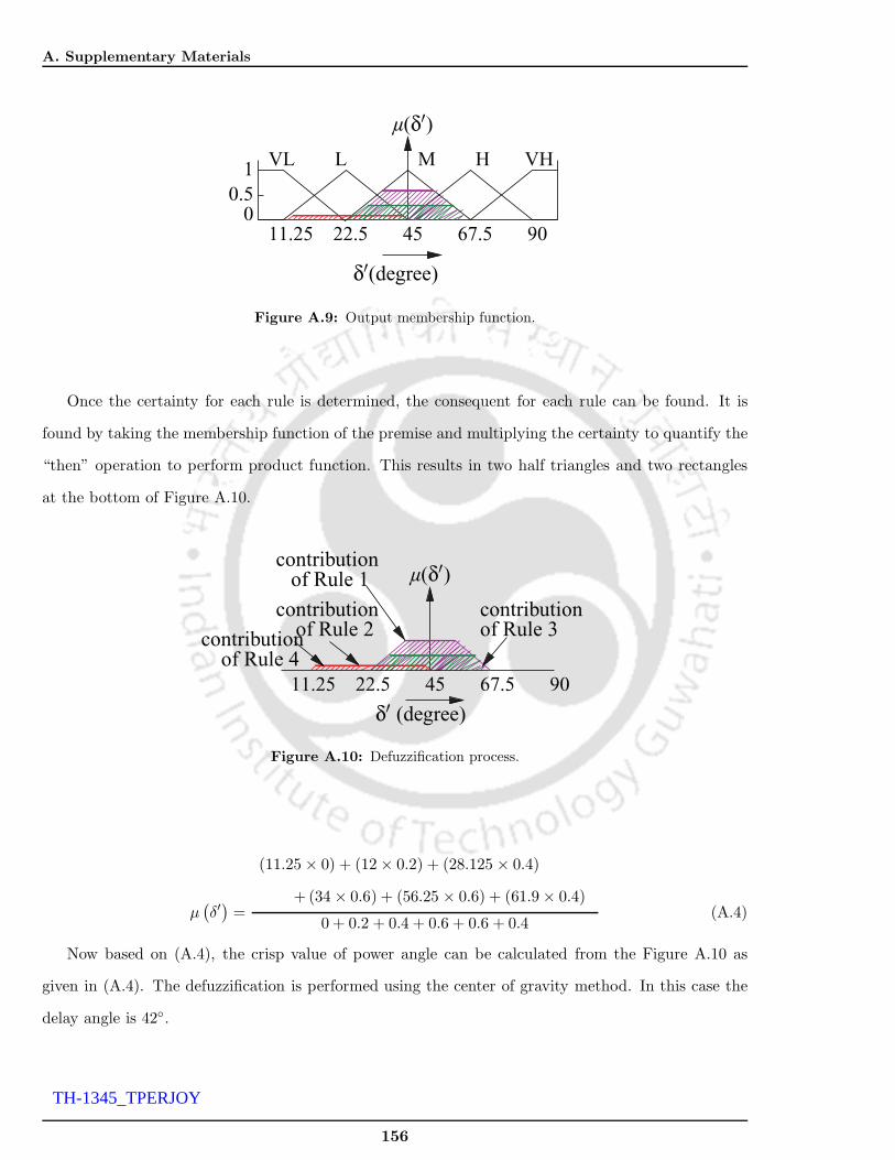
A. Supplementary Materials
1
0.50
22.5 45 9011.25 67.5
M H VHVL L
δ′(degree)
µ(δ′)
Figure A.9: Output membership function.
Once the certainty for each rule is determined, the consequent for each rule can be found. It is
found by taking the membership function of the premise and multiplying the certainty to quantify the
“then” operation to perform product function. This results in two half triangles and two rectangles
at the bottom of Figure A.10.
22.5 45 9011.25 67.5
of Rule 3of Rule 2
of Rule 4
of Rule 1
δ′ (degree)
µ(δ′)contribution
contributioncontribution
contribution
Figure A.10: Defuzzification process.
µ(δ′)
=
(11.25 × 0) + (12 × 0.2) + (28.125 × 0.4)
+ (34 × 0.6) + (56.25 × 0.6) + (61.9 × 0.4)
0 + 0.2 + 0.4 + 0.6 + 0.6 + 0.4(A.4)
Now based on (A.4), the crisp value of power angle can be calculated from the Figure A.10 as
given in (A.4). The defuzzification is performed using the center of gravity method. In this case the
delay angle is 42.
156
TH-1345_TPERJOY

A.5 Sample calculation for mutual inductance of Chapter 4
A.5 Sample calculation for mutual inductance of Chapter 4
This part describes the computation procedure of MI computation described in Chapter 4. The
following set of example considered details the calculation procedure. Consider two square coils of
length (L) and width (W) of 18cm having a conductor diameter of 1.83mm. The number of turns for
excitation (EC) and observation coils (OC) are 11 and 9 respectively. The current flow in EC is taken
to be 10A. The following cases of variations are chosen for explanation of analytical model.
Case I: Perfect alignment - vertical variation: OC kept at a vertical height of 2cm with respect
to EC.
Case II: Perfect alignment - planar variation: OC kept at a vertical height of 2.1cm and
rotated with an angle of 10.
Case III: Angular misalignment: The center to center distance between OC and EC is 12.8cm.
OC is tilted to an angle of 10 with respect to EC.
The numerical values obtained in each step for multiple turns of OC are summarized in Table A.3 for
the above considered cases. The flux linkage for each turn of OC is calculated using (4.8) and (4.9).
From these results, the total flux linkage and mutual inductance is calculated using (4.10) and (4.1).
Table A.3: Results for sample calculation.
SOClt
ϕ1 20.78 19.72 3.27 ϕ6 20.03 18.87 2.83
ϕ2 20.81 19.69 3.18 ϕ7 19.60 18.49 2.74
ϕ3 20.76 19.59 3.10 ϕ8 19.09 18.04 2.64
ϕ4 20.61 19.42 3.01 ϕ9 18.49 17.52 2.55
ϕ5 20.37 19.18 2.92
λ12 180.50 170.50 26.20
M 18.05µH 17.05µH 2.62µH
A.6 Remaining results of Chapter 5
This part has described the rest of the results from Chapter 5. Here the analysis explains to study
the operation of the converter at three different modes of frequencies.
• Converter operation at resonance frequency (f = fo)
• Converter operation above resonance frequency (f >fo)
157
TH-1345_TPERJOY
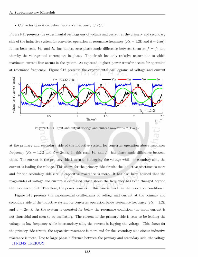
A. Supplementary Materials
• Converter operation below resonance frequency (f <fo)
Figure f-11 presents the experimental oscillograms of voltage and current at the primary and secondary
side of the inductive system for converter operation at resonance frequency (RL = 1.2Ω and d = 2cm).
It has been seen, Vin and Iin has almost zero phase angle difference between them at f = fo and
thereby the voltage and current are in phase. The circuit has only resistive nature due to which
maximum current flow occurs in the system. As expected, highest power transfer occurs for operation
at resonance frequency. Figure f-12 presents the experimental oscillograms of voltage and current
0 0.5 1 1.5 2 2.5
x 10−4
−5
0
5
Time (s)
Vol
tage
(vo
lts),
cur
rent
(am
ps)
Vin Iin Vo Iof = 15.432 kHz
RL = 1.2 Ω
Figure f-11: Input and output voltage and current waveforms at f = fo.
at the primary and secondary side of the inductive system for converter operation above resonance
frequency (RL = 1.2Ω and d = 2cm). In this case, Vin and Iin has phase angle difference between
them. The current in the primary side is seen to be lagging the voltage while in secondary side, the
current is leading the voltage. This shows for the primary side circuit, the inductive reactance is more
and for the secondary side circuit capacitive reactance is more. It has also been noticed that the
magnitudes of voltage and current is decreased which shows the frequency has been changed beyond
the resonance point. Therefore, the power transfer in this case is less than the resonance condition.
Figure f-13 presents the experimental oscillograms of voltage and current at the primary and
secondary side of the inductive system for converter operation below resonance frequency (RL = 1.2Ω
and d = 2cm). As the system is operated far below the resonance condition, the input current is
not sinusoidal and seen to be oscillating. The current in the primary side is seen to be leading the
voltage at low frequency while in secondary side, the current is lagging the voltage. This shows for
the primary side circuit, the capacitive reactance is more and for the secondary side circuit inductive
reactance is more. Due to large phase difference between the primary and secondary side, the voltage
158
TH-1345_TPERJOY

A.6 Remaining results of Chapter 5
0 0.2 0.4 0.6 0.8 1 1.2
x 10−4
−5
0
5
Time (s)
Vol
tage
(vo
lts),
cur
rent
(am
ps)
Vin Iin Vo Iof = 30 kHz
RL = 1.2 Ω
Figure f-12: Input and output voltage and current waveforms at f>fo.
induced in the secondary side coil is less and the efficiency in this case is also got reduced.
0 1 2 3 4 5 6 7
x 10−4
−10
−5
0
5
10
Time (s)
Vol
tage
(vo
lts),
cur
rent
(am
ps)
Vin Iin Vo Iof = 5.8 kHz
RL = 1.2 Ω
Figure f-13: Input and output voltage and current waveforms at f<fo.
Figure f-14 shows the comparison of efficiency for four compensations at distance 4cm and RL =
1.2Ω. As explained, SS and PS topology has higher efficiency than SP and PP compensation. However,
when compared at D=2cm the efficiency got reduced to 50% at distance 4cm and is further reduced
for higher frequencies. This is because at higher distance causes leakage flux more than the main flux
linkage due to larger air gap between the coils.
Figure f-15 shows the comparison of efficiency at 20kHz operating frequency for variable air gap
distance of four compensation topology. The performance characteristics of efficiency curve is almost
similar to the optimum resonance condition. This is because, the system has an operating range and
it has higher efficiency in and around resonance condition. If the circuit goes far beyond the resonance
point i.e. too higher or lower, the efficiency gradually falls. This necessitates the requirement of
159
TH-1345_TPERJOY

A. Supplementary Materials
0 2 4 6 8 10 12 14 16 18
x 104
0
5
10
15
20
25
30
35
40
45
50
Frequency (Hz)
Effi
cien
cy (
%)
SS SP PS PP
Figure f-14: Efficiency versus frequency at d=4cm, RL = 1.2Ω.
frequency control in the CPT system.
2 3 4 5 6 7 8 9 100
10
20
30
40
50
60
70
80
Distance (cm)
Effi
cien
cy (
%)
SS SP PS PP
Figure f-15: Efficiency versus distance at f=20kHz, RL = 1.2Ω.
Figure f-16 shows the efficiency plot for variable load resistance at distance 4cm. As explained
above, the efficiency of the system is less at higher distance due to large air gap. The leakage flux in
the system is more than the main flux linked in the secondary. Furthermore, the impedance of the
system changes due to which the efficiency of the system has changed.
160
TH-1345_TPERJOY

A.6 Remaining results of Chapter 5
0 5 10 15 20 25 30 3510
15
20
25
30
35
40
45
50
55
Load resistance (Ω)
Effi
cien
cy (
%)
SS SP PS PP
Figure f-16: Efficiency versus load resistance at d=4cm, f=15.432kHz.
161
TH-1345_TPERJOY

A. Supplementary Materials
162
TH-1345_TPERJOY

Bibliography
[1] M. Kisacikoglu, B. Ozpineci, and L. Tolbert, “Ev/phev bidirectional charger assessment for v2g reactivepower operation,” IEEE Transn. on Power Electron., vol. 28, no. 12, pp. 5717–5727, Dec 2013.
[2] M. Yilmaz and P. Krein, “Review of battery charger topologies, charging power levels, and infrastructurefor plug-in electric and hybrid vehicles,” IEEE Transn. on Power Electron., vol. 28, no. 5, pp. 2151–2169,May 2013.
[3] D. Mayfield, “Siting electric vehicle charging stations,” Sust. Transp. Strat., Clean Fuels Ohio, Apr. 2012.
[4] “Electric vehicle charging infrastructure deployment guidelines for the oregon i-5 metro areas of portland,salem, corvallis and eugene,” Electric Transp. Eng. corp., Ecotality Company, Apr. 2010.
[5] “Residential electric vehicle (ev) charger guidelines,” City of Riverside Building and Safety Division,ECOtality Company, Dec. 2012.
[6] D. Mayfield, “Selectric vehicle charging for persons with disabilities,” Sust. Transp. Strat., Clean FuelsOhio, Feb. 2012.
[7] “Long-range ev charging infrastructure plan for western oregon,” City of Riverside Building and SafetyDivision, ECOtality Company, Aug. 2010.
[8] D. Mayfield, “Site design for electric vehicle charging stations,” Sust. Transp. Strat., Clean Fuels Ohio,Jul. 2012.
[9] “Electric vehicle charging stations technical installation guide,” Sust. Transp. Strat., Hydro-Quebec, Jan.2012.
[10] G. Pistoia, Electric and Hybrid Vehicles power sources, Models, sustainability, infrastructure and themarket. Elsev. Scien. and Tech. Rights, 2010.
[11] J. Larminie and J. Lowry, Electric Vehicle Technology Explained. John Wiley and Sons Ltd., 2003.
[12] M. Ehsani, Y. Gao, S. E.Gay, and A. Emadi, Modern Electric, Hybrid Electric and Fuel Cell Vehicles,Fundamentals Theory and Design, M. H. Rashid, Ed. CRC Press, 2005.
[13] Z. Liu, F. Wen, and G. Ledwich, “Optimal planning of electric-vehicle charging stations in distributionsystems,” IEEE Trans. on Pow. Deliv., vol. 28, no. 1, pp. 102–110, 2013.
[14] J. L. Villa, J. Sallan, A. Llombart, and J. F. Sanz, “Design of a high frequency inductively coupled powertransfer system for electric vehicle battery charge,” Appl. Ener., vol. 86, no. 3, pp. 355 – 363, 2009.
[15] M. F. M. Elias, K. M. Nor, N. Rahim, and A. K. Arof, “Lithium-ion battery charger for high energyapplication,” Nation. Pow. Eng. Conf., pp. 283–288, 2003.
[16] S. Bai and S. Lukic, “Unified active filter and energy storage system for an mw electric vehicle chargingstation,” IEEE Trans. on Pow. Electron., vol. 28, no. 12, pp. 5793–5803, Dec 2013.
[17] M. Etezadi-Amoli, K. Choma, and J. Stefani, “Rapid-charge electric-vehicle stations,” IEEE Trans. onPow. Deliv., vol. 25, no. 3, pp. 1883–1887, 2010.
[18] S. Haghbin, S. Lundmark, M. Alakula, and O. Carlson, “Grid-connected integrated battery chargers invehicle applications: Review and new solution,” IEEE Trans. on Ind. Electron., vol. 60, no. 2, pp. 459–473,2013.
163
TH-1345_TPERJOY

BIBLIOGRAPHY
[19] X. Zhou, S. Lukic, S. Bhattacharya, and A. Huang, “Design and control of grid-connected converter inbi-directional battery charger for plug-in hybrid electric vehicle application,” IEEE Veh. Pow. and Propul.Conf. VPPC ’09., pp. 1716–1721, 2009.
[20] K. Young, C. Wang, L. Wang, and K. Strunz, “Electric vehicle battery technolo-gies,” Electric Veh. Integ. into Modern Pow. Net., pp. 15–56, 2013. [Online]. Available:http://dx.doi.org/10.1007/978-1-4614-0134-6 2.
[21] S. Chopra and P. Bauer, “Driving range extension of ev with on-road contactless power transfer x2014;acase study,” IEEE Trans. on Ind. Electron., vol. 60, no. 1, pp. 329–338, 2013.
[22] C.-S. Wang, G. Covic, and O. Stielau, “Power transfer capability and bifurcation phenomena of looselycoupled inductive power transfer systems,” IEEE Trans. on Ind. Electron., vol. 51, no. 1, pp. 148–157,2004.
[23] C.-S. Wang, O. Stielau, and G. Covic, “Design considerations for a contactless electric vehicle batterycharger,” IEEE Transn. on Ind. Electron., vol. 52, no. 5, pp. 1308–1314, Oct 2005.
[24] H. Bergner, K. Hempel, and G. Sargsjan, “Contactless detection of optical induced current in microelec-tronic devices by capacitive coupling,” Microelectron. Eng., vol. 2, no. 4, pp. 115 – 122, 1996.
[25] M. Koerdel, F. Alatas, A. Schick, S. Rupitsch, and R. Lerch, “Contactless inspection of planar electronicdevices by capacitive coupling: Development of a model describing the sensor signal and its impact onsignal post-processing,” Sensors and Actuators A: Physical, vol. 172, no. 1, pp. 88 – 97, 2011.
[26] A. Hu, C. Liu, and H. L. Li, “A novel contactless battery charging system for soccer playing robot,” 15thIntern. Conf. on Mech. and Mach. Vision in Practice, pp. 646–650, 2008.
[27] M. Kline, I. Izyumin, B. Boser, and S. Sanders, “Capacitive power transfer for contactless charging,”Twenty-Sixth IEEE Ann. Appl. Pow. Electron. Conf. and Exposit. (APEC), pp. 1398–1404, 2011.
[28] C. Liu, A. Hu, and X. Dai, “A contactless power transfer system with capacitively coupled matrix pad,”IEEE Ener. Conv. Cong. and Exposit.(ECCE), pp. 3488–3494, 2011.
[29] W. P. Choi, W. C. Ho, X. Liu, and S. Hui, “Comparative study on power conversion methods for wirelessbattery charging platform,” 14th Intern. Pow. Electron. and Mot. Cont. Conf. (EPE/PEMC), pp. S15–9–S15–16, 2010.
[30] E. Joy, A. Dalal, and P. Kumar, “The accurate computation of mutual inductance of two air core squarecoils with lateral and angular misalignments in a flat planar surface,” IEEE Trans. on Mag., pp. 1–9, Jan.2014.
[31] J. Villa, J. Sallan, J. Sanz Osorio, and A. Llombart, “High-misalignment tolerant compensation topologyfor icpt systems,” IEEE Trans. on Ind. Electron., vol. 59, no. 2, pp. 945–951, Feb. 2012.
[32] S. Xun Liu ; Shatin ; Hui, “Simulation study and experimental verification of a universal contactlessbattery charging platform with localized charging features,” IEEE Trans. on Power Electron., vol. 22,no. 6, pp. 2202 – 2210, Nov. 2007.
[33] X. . H. S. Zhong, W.X. ; Kowloon; Liu, “A novel single-layer winding array and receiver coil structure forcontactless battery charging systems with free-positioning and localized charging features,” IEEE Trans.on Ind. Electron., vol. 58, no. 9, pp. 4136 – 4144, Sept. 2011.
[34] C. Mecke, R.; Rathge, “High frequency resonant inverter for contactless energy transmission over largeair gap,” IEEE 35th Ann. (Volume:3 ) Power Electron. Specia. Conf., PESC 04., vol. 58, no. 9, pp. 1737– 1743, June. 2004.
[35] J. T. Boys, G. A. Covic, and A. W. Green, “Stability and control of inductively coupled power transfersystems,” Electric Power Applications, IEE Proceedings -, vol. 147, no. 1, pp. 37–43, Jan. 2000.
[36] J. Sallan, J. Villa, A. Llombart, and J. Sanz, “Optimal design of icpt systems applied to electric vehiclebattery charge,” IEEE Transn. on Ind. Electron., vol. 56, no. 6, pp. 2140–2149, June 2009.
[37] X. Liu and S. Hui, “Optimal design of a hybrid winding structure for planar contactless battery chargingplatform,” IEEE Trans. on Power Electron., vol. 23, no. 1, pp. 455–463, Jan 2008.
164
TH-1345_TPERJOY

BIBLIOGRAPHY
[38] M. Budhia, G. Covic, and J. Boys, “Magnetic design of a three-phase inductive power transfer system forroadway powered electric vehicles,” pp. 1–6, Sept 2010.
[39] D. K. Cheng, Field and Wave Electromagnetics, 2nd ed., ser. The Addison-Wesley series in electrical engineering. Addison-Wesley, Jan. 1989. [Online]. Available:http://www.amazon.com/exec/obidos/redirect?tag=citeulike07-20\&path=ASIN/0201128195
[40] C. Zhou, K. Qian, M. Allan, and W. Zhou, “Modeling of the cost of ev battery wear due to v2g applicationin power systems,” IEEE Trans. on Ener. Conv., vol. 26, no. 4, pp. 1041–1050, 2011.
[41] C. Rathge and D. Kuschner, “High efficient inductive energy and data transmission system with specialcoil geometry,” 13th Europ. Conf. on Pow. Electron. and Appln, EPE ’09., pp. 1–8, Sept. 2009.
[42] J. Shin, S. Shin, Y. Kim, S. Ahn, S. Lee, G. Jung, S. Jeon, and D. Cho, “Design and implementationof shaped magnetic resonance based wireless power transfer system for roadway-powered moving electricvehicles,” IEEE Trans. on Ind. Electron., vol. PP, no. 99, pp. 1–1, March 2013.
[43] A. Kelley and W. Owens, “Connectorless power supply for an aircraft-passenger entertainment system,”IEEE Trans. on Pow. Electron., vol. 4, no. 3, pp. 348–354, Jul. 1989.
[44] J. Barnard, J. Ferreira, and J. Van Wyk, “Sliding transformers for linear contactless power delivery,”IEEE Trans. on Ind. Electron., vol. 44, no. 6, pp. 774–779, Dec. 1997.
[45] C.-G. Kim, D.-H. Seo, J.-S. You, J.-H. Park, and B. H. Cho, “Design of a contactless battery charger forcellular phone,” IEEE Trans. on Ind. Electron., vol. 48, no. 6, pp. 1238–1247, Dec. 2001.
[46] T. Bieler, M. Perrottet, V. Nguyen, and Y. Perriard, “Contactless power and information transmission,”IEEE Trans. on Ind. Appln., vol. 38, no. 5, pp. 1266–1272, Sept/Oct. 2002.
[47] Y. Jang and M. Jovanovic, “A contactless electrical energy transmission system for portable-telephonebattery chargers,” IEEE Trans. on Ind. Electron., vol. 50, no. 3, pp. 520–527, June 2003.
[48] G. A. J. Elliott, G. Covic, D. Kacprzak, and J. Boys, “A new concept: Asymmetrical pick-ups forinductively coupled power transfer monorail systems,” IEEE Trans. on Magn., vol. 42, no. 10, pp. 3389–3391, Oct. 2006.
[49] J. Casanova, Z. N. Low, and J. Lin, “Design and optimization of a class-e amplifier for a loosely coupledplanar wireless power system,” IEEE Trans. on Circ. and Sys. II: Express Briefs,, vol. 56, no. 11, pp.830–834, Nov. 2009.
[50] D. A. G. Pedder, A. Brown, and J. Skinner, “A contactless electrical energy transmission system,” IEEETrans. on Ind. Electron., vol. 46, no. 1, pp. 23–30, Feb. 1999.
[51] U. Madawala and D. Thrimawithana, “A bidirectional inductive power interface for electric vehicles inv2g systems,” IEEE Trans. on Ind. Electron., vol. 58, no. 10, pp. 4789–4796, Oct 2011.
[52] M. Kisacikoglu, B. Ozpineci, and L. Tolbert, “Examination of a phev bidirectional charger system forv2g reactive power compensation,” IEEE Twenty-Fifth Ann. Appl. Pow. Electron. Conf. and Exposit.(APEC), pp. 458–465, 2010.
[53] C. Tang, X. Dai, Z. Wang, Y. Su, and Y. Sun, “A bidirectional contactless power transfer system withdual-side power flow control,” pp. 1–6, Oct 2012.
[54] A. Swain, M. Neath, U. Madawala, and D. Thrimawithana, “A dynamic multivariable state-space modelfor bidirectional inductive power transfer systems,” IEEE Trans. on Pow. Electron., vol. 27, no. 11, pp.4772–4780, 2012.
[55] C. Guille and G. Gross, “Design of a conceptual framework for the v2g implementation,” IEEE Ener.2030 Conf., pp. 1–3, 2008.
[56] D. P. Ghosh, R. J. Thomas, and S. B. Wicker, “A privacy-aware design for the vehicle-to-grid framework,”46th Hawaii Inter. Conf. on Sys. Scien. (HICSS), pp. 2283–2291, 2013.
[57] Y. Ota, H. Taniguchi, T. Nakajima, K. Liyanage, J. Baba, and A. Yokoyama, “Autonomous distributedv2g (vehicle-to-grid) satisfying scheduled charging,” IEEE Trans. on Smart Grid, vol. 3, no. 1, pp. 559–564, 2012.
165
TH-1345_TPERJOY

BIBLIOGRAPHY
[58] E. Sortomme and M. El-Sharkawi, “Optimal scheduling of vehicle-to-grid energy and ancillary services,”IEEE Trans. on Smart Grid, vol. 3, no. 1, pp. 351–359, 2012.
[59] Z. Darabi and M. Ferdowsi, “Aggregated impact of plug-in hybrid electric vehicles on electricity demandprofile,” IEEE Trans. on Sust. Ener., vol. 2, no. 4, pp. 501–508, 2011.
[60] J. Pillai and B. Bak-Jensen, “Integration of vehicle-to-grid in the western danish power system,” IEEETrans. on Sust. Ener., vol. 2, no. 1, pp. 12–19, 2011.
[61] H. Guo, Y. Wu, F. Bao, H. Chen, and M. Ma, “Ubapv2g: A unique batch authentication protocol forvehicle-to-grid communications,” IEEE Trans. on Smart Grid, vol. 2, no. 4, pp. 707–714, 2011.
[62] T. Mishima, K. Akamatsu, and M. Nakaoka, “A high frequency-link secondary-side phase-shifted full-range soft-switching pwm dc-dc converter with zcs active rectifier for ev battery chargers,” IEEE Transn.on Power Electron., vol. 28, no. 12, pp. 5758–5773, Dec 2013.
[63] C.-Y. Oh, D.-H. Kim, D.-G. Woo, W.-Y. Sung, Y.-S. Kim, and B.-K. Lee, “A high-efficient nonisolatedsingle-stage on-board battery charger for electric vehicles,” IEEE Transn. on Power Electron., vol. 28,no. 12, pp. 5746–5757, Dec 2013.
[64] B. Gu, J.-S. Lai, N. Kees, and C. Zheng, “Hybrid-switching full-bridge dc dc converter with minimalvoltage stress of bridge rectifier, reduced circulating losses, and filter requirement for electric vehiclebattery chargers,” IEEE Transn. on Power Electron., vol. 28, no. 3, pp. 1132–1144, March 2013.
[65] S. Deilami, A. Masoum, P. Moses, and M. Masoum, “Real-time coordination of plug-in electric vehiclecharging in smart grids to minimize power losses and improve voltage profile,” IEEE Trans. Smart Grid,vol. 2, no. 3, pp. 456–467, Sept. 2011.
[66] A. Masoum, S. Deilami, P. Moses, M. Masoum, and A. Abu-siada, “Smart load management of plug-inelectric vehicles in distribution and residential networks with charging stations for peak shaving and lossminimisation considering voltage regulation,” IET Generation, Transmission Distribution, vol. 5, no. 8,pp. 877–888, August 2011.
[67] R. Crosier, S. Wang, and M. Jamshidi, “A 4800-v grid-connected electric vehicle charging station thatprovides stacom-apf functions with a bi-directional, multi-level, cascaded converter,” pp. 1508–1515, Feb2012.
[68] S. Babic and C. Akyel, “New formulas for mutual inductance and axial magnetic force between magnet-ically coupled coils: Thick circular coil of the rectangular cross-section-thin disk coil (pancake),” IEEETrans. on Magn., vol. 49, no. 2, pp. 860–868, Feb. 2013.
[69] T. Ho, B. Gomersall, and L. Ran, “Contactless charging for electric vehicles with a large air gap,” Proceed.of Europ. Conf. on Pow. Electron. and Appln(EPE 2011), pp. 1–10, 2011.
[70] J. Wang, S. Ho, W. Fu, and M. Sun, “Analytical design study of a novel witricity charger with lateral andangular misalignments for efficient wireless energy transmission,” IEEE Trans. Magn., vol. 47, no. 10, pp.2616 –2619, Oct. 2011.
[71] C.-S. Wang, G. Covic, and O. Stielau, “General stability criterions for zero phase angle controlled looselycoupled inductive power transfer systems,” 27th IEEE Ann. Conf. of Ind. Electron. Soc. (IECON), vol. 2,pp. 1049–1054 vol.2, 2001.
[72] M. Khan, I. Husain, and Y. Sozer, “Integrated electric motor drive and power electronics for bidirectionalpower flow between the electric vehicle and dc or ac grid,” IEEE Transn. on Power Electron., vol. 28,no. 12, pp. 5774–5783, Dec 2013.
[73] K. Clement-Nyns, E. Haesen, and J. Driesen, “The impact of charging plug-in hybrid electric vehicles ona residential distribution grid,” IEEE Trans. on Power Sys., vol. 25, no. 1, pp. 371–380, Feb. 2010.
[74] Z. Yang, S. Yu, W. Lou, and C. Liu, “Privacy-preserving communication and precise reward architecturefor V2G networks in smart grid,” IEEE Trans. Smart Grid, vol. 2, no. 4, pp. 697–706, Dec. 2011.
[75] N. Rotering and M. Ilic, “Optimal charge control of plug-in hybrid electric vehicles in deregulated elec-tricity markets,” IEEE Trans. Power Syst., vol. 26, no. 3, pp. 1021–1029, Aug. 2011.
166
TH-1345_TPERJOY

BIBLIOGRAPHY
[76] S. Bifaretti, P. Zanchetta, A. Watson, L. Tarisciotti, and J. Clare, “Advanced power electronic conversionand control system for universal and flexible power management,” IEEE Transn. on Smart Grid, vol. 2,no. 2, pp. 231–243, June 2011.
[77] G. Capizzi, F. Bonanno, and G. Tina, “Recurrent neural network-based modeling and simulation oflead-acid batteries charge discharge,” IEEE Trans. on Energ. Conv., vol. 26, no. 2, pp. 435–443, June2011.
[78] V. Agarwal, K. Uthaichana, R. DeCarlo, and L. Tsoukalas, “Development and validation of a batterymodel useful for discharging and charging power control and lifetime estimation,” IEEE Trans. on Energ.Conv., vol. 25, no. 3, pp. 821–835, Sept 2010.
[79] K. Thirugnanam, J. Ezhil Reena, M. Singh, and P. Kumar, “Mathematical modeling of li-ion batteryusing genetic algorithm approach for v2g applications,” IEEE Trans. on Energ. Conversn., vol. 29, no. 2,pp. 332–343, June 2014.
[80] S. Han, S. Han, and K. Sezaki, “Development of an optimal vehicle-to-grid aggregator for frequencyregulation,” IEEE Trans. on Smart Grid, vol. 1, no. 1, pp. 65–72, June 2010.
[81] ——, “Estimation of achievable power capacity from plug-in electric vehicles for V2G frequency regulation:Case studies for market participation,” IEEE Trans. Smart Grid, vol. 2, no. 4, pp. 632–641, Dec. 2011.
[82] H. Liu, Z. Hu, Y. Song, and J. Lin, “Decentralized vehicle-to-grid control for primary frequency regulationconsidering charging demands,” IEEE Trans. Power Syst., vol. 28, no. 3, pp. 3480–3489, Aug. 2013.
[83] J. Escudero-Garzas, A. Garcia-Armada, and G. Seco-Granados, “Fair design of plug-in electric vehiclesaggregator for v2g regulation,” IEEE Trans. Veh. Technol., vol. 61, no. 8, pp. 3406–3419, Oct. 2012.
[84] C. Evangelista, F. Valenciaga, and P. Puleston, “Active and reactive power control for wind turbine basedon a mimo 2-sliding mode algorithm with variable gains,” IEEE Trans. on Energ. Conv., vol. 28, no. 3,pp. 682–689, Sept 2013.
[85] S. M. A. Cruz, “An active reactive power method for the diagnosis of rotor faults in three-phase inductionmotors operating under time-varying load conditions,” IEEE Trans. on Energ. Conv., vol. 27, no. 1, pp.71–84, March 2012.
[86] A. Moawwad, V. Khadkikar, and J. Kirtley, “A new P-Q-V droop control method for an interline photo-voltaic (I-PV) power system,” IEEE Trans. on Power Deliv., vol. 28, no. 2, pp. 658–668, April 2013.
[87] M. Singh, P. Kumar, and I. Kar, “Implementation of vehicle to grid infrastructure using fuzzy logiccontroller,” IEEE Trans. on Smart Grid, vol. 3, no. 1, pp. 565–577, March 2012.
[88] P. M. S. Carvalho, P. F. Correia, and L. Ferreira, “Distributed reactive power generation control forvoltage rise mitigation in distribution networks,” IEEE Trans. on Power Sys., vol. 23, no. 2, pp. 766–772,May 2008.
[89] R. H. Liang and Y. S. Wang, “Fuzzy-based reactive power and voltage control in a distribution system,”IEEE Trans. on Power Deliv., vol. 22, no. 12, pp. 64–64, Dec 2002.
[90] M. Helmbrecht, C. Olaverri-Monreal, K. Bengler, R. Vilimek, and A. Keinath, “How electric vehiclesaffect driving behavioral patterns,” IEEE Intell. Transp. Sys Magaz., vol. 6, no. 3, pp. 22–32, Fall 2014.
[91] Z. Duan, B. Gutierrez, and L. Wang, “Forecasting plug-in electric vehicle sales and the diurnal rechargingload curve,” IEEE Trans. on Smart Grid, vol. 5, no. 1, pp. 527–535, Jan 2014.
[92] Y. Ma, T. Houghton, A. Cruden, and D. Infield, “Modeling the benefits of vehicle-to-grid technology toa power system,” IEEE Trans. on Power Systm., vol. 27, no. 2, pp. 1012–1020, May 2012.
[93] S. Han, S. Han, and K. Sezaki, “Estimation of achievable power capacity from plug-in electric vehiclesfor v2g frequency regulation: Case studies for market participation,” IEEE Trans. on Smart Grid, vol. 2,no. 4, pp. 632–641, Dec 2011.
[94] T. Ezhil Reena Joy, K. Thirugnanam, and P. Kumar, “A novel reduced switch count bidirectional contact-less charging system for evs and phevs applications,” IEEE Students Confer.on Enging.and Sys. (SCES),pp. 1–6, 2013.
167
TH-1345_TPERJOY

BIBLIOGRAPHY
[95] Y. He, B. Venkatesh, and L. Guan, “Optimal scheduling for charging and discharging of electric vehicles,”IEEE Trans. on Smart Grid, vol. 3, no. 3, pp. 1095–1105, Sept 2012.
[96] D. Wu, D. Aliprantis, and L. Ying, “Load scheduling and dispatch for aggregators of plug-in electricvehicles,” IEEE Trans. on Smart Grid, vol. 3, no. 1, pp. 368–376, March 2012.
[97] C.-Y. Oh, D.-H. Kim, D.-G. Woo, W.-Y. Sung, Y.-S. Kim, and B.-K. Lee, “A high-efficient nonisolatedsingle-stage on-board battery charger for electric vehicles,” IEEE Transn. on Power Electron., vol. 28,no. 12, pp. 5746–5757, Dec 2013.
[98] R. Metidji, B. Metidji, and B. Mendil, “Design and implementation of a unity power factor fuzzy batterycharger using an ultrasparse matrix rectifier,” IEEE Transn. on Power Electron., vol. 28, no. 5, pp.2269–2276, May 2013.
[99] R. . S. W. Crosier, “Dq- frame modeling of an active power filter integrated with a grid connectedmultifunctional electric vehcile charging station,” IEEE Transn. on Power Electron., 2013.
[100] F.-J. Lin, M.-S. Huang, P.-Y. Yeh, H.-C. Tsai, and C.-H. Kuan, “Dsp-based probabilistic fuzzy neuralnetwork control for li-ion battery charger,” IEEE Transn. on Power Electron., vol. 27, no. 8, pp. 3782–3794, Aug 2012.
[101] J. Traube, F. Lu, D. Maksimovic, J. Mossoba, M. Kromer, P. Faill, S. Katz, B. Borowy, S. Nichols, andL. Casey, “Mitigation of solar irradiance intermittency in photovoltaic power systems with integratedelectric-vehicle charging functionality,” IEEE Transn. on Power Electron., vol. 28, no. 6, pp. 3058–3067,June 2013.
[102] G. Carli and S. Williamson, “Technical considerations on power conversion for electric and plug-in hybridelectric vehicle battery charging in photovoltaic installations,” IEEE Transn. on Power Electron., vol. 28,no. 12, pp. 5784–5792, Dec 2013.
[103] K. Aditya and S. S. Williamson, “Design considerations for loosely coupled inductive power transfer (ipt)system for electric vehicle battery charging a comprehensive review,” IEEE Transptn. Electrific. Conf.and Expo (ITEC), 2014, June 2014.
[104] J. Hayes, M. Egan, J. M. D. Murphy, S. Schulz, and J. Hall, “Wide-load-range resonant converter supplyingthe sae j-1773 electric vehicle inductive charging interface,” IEEE Transn. on Industry Appln., vol. 35,no. 4, pp. 884–895, Jul 1999.
[105] G. Covic, J. Boys, M. Kissin, and H. Lu, “A three-phase inductive power transfer system for roadway-powered vehicles,” IEEE Transn. on Ind. Electron., vol. 54, no. 6, pp. 3370–3378, Dec 2007.
[106] D. Thrimawithana and U. Madawala, “A three-phase bi-directional ipt system for contactless charging ofelectric vehicles,” pp. 1957–1962, June 2011.
[107] D. Thrimawithana and U. Madawala, “A novel matrix converter based bi-directional ipt power interfacefor v2g applications,” pp. 495–500, Dec 2010.
[108] S. Nakadachi, S. Mochizuki, S. Sakaino, Y. Kaneko, S. Abe, and T. Yasuda, “Bidirectional contactlesspower transfer system expandable from unidirectional system,” pp. 3651–3657, Sept 2013.
[109] H. Li, A. Hu, G. Covic, and C. Tang, “A new primary power regulation method for contactless powertransfer,” pp. 1–5, Feb 2009.
[110] M. H. Rashid, Power Electronics Circuits Devices and Applications, second edition ed. Pearson Education,2004.
[111] S. Babic, F. Sirois, C. Akyel, G. Lemarquand, V. Lemarquand, and R. Ravaud, “New formulas for mutualinductance and axial magnetic force between a thin wall solenoid and a thick circular coil of rectangularcross-section,” IEEE Trans. Magn., vol. 47, no. 8, pp. 2034 –2044, Aug. 2011.
[112] Y. Su, X. Liu, and S. Hui, “Mutual inductance calculation of movable planar coils on parallel surfaces,”IEEE Trans.Power Electron., vol. 24, no. 4, pp. 1115 –1123, April 2009.
[113] M. Soma, D. C. Galbraith, and R. L. White, “Radio-frequency coils in implantable devices: Misalignmentanalysis and design procedure,” IEEE Trans. Biomed. Eng., vol. BME-34, no. 4, pp. 276 –282, April 1987.
168
TH-1345_TPERJOY

BIBLIOGRAPHY
[114] S. Hui, H. Chung, and S. Tang, “Coreless pcb-based transformers for power mosfet/igbt gate drive cir-cuits,” 28th Ann. IEEE Power Electron. Spec. Conf., PESC97, vol. 2, pp. 1171 –1176, Jun 1997.
[115] F. Grover, Inductances calculations. Dover Pulications, News York, 1964.
[116] T. Engel and D. Mueller, “High-speed and high-accuracy method of mutual-inductance calculations,”IEEE Trans. Plas. Scien., vol. 37, no. 5, pp. 683 –692, May 2009.
[117] S. Babic and C. Akyel, “Calculating mutual inductance between circular coils with inclined axes in air,”IEEE Trans.Magn., vol. 44, no. 7, pp. 1743 –1750, July 2008.
[118] T. H. Fawzi and P. E. Burke, “The accurate computation of self and mutual inductances of circular coils,”IEEE Trans. Power Apparatus and Systm., vol. PAS-97, no. 2, pp. 464 –468, March 1978.
[119] T. Engel and S. Rohe, “A comparison of single-layer coaxial coil mutual inductance calculations usingfinite-element and tabulated methods,” IEEE Tran. Magnetics., vol. 42, no. 9, pp. 2159 –2163, Sept. 2006.
[120] D. Zhang and C. S. Koh, “An efficient semianalytic computation method of magnetic field for a circularcoil with rectangular cross section,” IEEE Trans. Magn., vol. 48, no. 1, pp. 62 –68, Jan. 2012.
[121] J. Conway, “Noncoaxial inductance calculations without the vector potential for axisymmetric coils andplanar coils,” IEEE Trans.Magn., vol. 44, no. 4, pp. 453 –462, Apr. 2008.
[122] S. Babic and C. Akyel, “Improvement in calculation of the self- and mutual inductance of thin-wallsolenoids and disk coils,” IEEE Trans. Magn., vol. 36, no. 4, pp. 1970 – 1975, July 2000.
[123] S. Babic, C. Akyel, and S. Salon, “New procedures for calculating the mutual inductance of the system:filamentary circular coil-massive circular solenoid,” IEEE Trans.Magn., vol. 39, no. 3, pp. 1131 – 1134,May 2003.
[124] S. Babic, S. Salon, and C. Akyel, “The mutual inductance of two thin coaxial disk coils in air,” IEEETrans. Magn., vol. 40, no. 2, pp. 822 – 825, March 2004.
[125] J. Conway, “Inductance calculations for circular coils of rectangular cross section and parallel axes usingbessel and struve functions,” IEEE Trans.Magn., vol. 46, no. 1, pp. 75 –81, Jan. 2010.
[126] J.T. Conway,, “Exact solutions for the mutual inductance of circular coils and elliptic coils,” IEEETrans.Magn., vol. 48, no. 1, pp. 81 –94, Jan. 2012.
[127] L. Forbes, S. Crozier, and D. Doddrell, “Rapid computation of static fields produced by thick circularsolenoids,” IEEE Trans. Magn., vol. 33, no. 5, pp. 4405 –4410, Sept. 1997.
[128] R. Ravaud, G. Lemarquand, S. Babic, V. Lemarquand, and C. Akyel, “Cylindrical magnets and coils:Fields, forces, and inductances,” IEEE Trans. Magn., vol. 46, no. 9, pp. 3585 –3590, Sept. 2010.
[129] J. de Boeij, E. Lomonova, and A. Vandenput, “Contactless energy transfer to a moving load part i:Topology synthesis and fem simulation,” IEEE Intern. Symp. on Ind. Electron., vol. 2, pp. 739 –744, July2006.
[130] J. L. Villa, J. Salln, A. Llombart, and J. F. Sanz, “Design of a high frequency inductively coupled powertransfer system for electric vehicle battery charge,” Applied Energy, Jun.
[131] K. O’Brien, G. Scheible, and H. Gueldner, “Design of large air-gap transformers for wireless power sup-plies,” 34th Ann. Power Electron. Spec. Conf., vol. 4, pp. 1557 – 1562, June 2003.
[132] X. Liu and S. Hui, “Optimal design of a hybrid winding structure for planar contactless battery chargingplatform,” IEEE Trans. on Power Electron., vol. 5, no. 1, pp. 455–463, Jan. 2006.
[133] E. Joy, B. Kushwaha, G. Rituraj, and P. Kumar, “Impact of circuit parameters in contactless powertransfer system,” IEEE International Conf. on Power Electron., Drives and Energ. Systems Conf., 2014.
[134] G. Rituraj, E. Joy, B. Kushwaha, and P. Kumar, “Analysis and comparison of series-series and series -parallel topology for contactless power transfer systems,” IEEE TENCON Conf., 2014.
[135] E. Joy, B. Kushwaha, G. Rituraj, and P. Kumar, “Analysis and comparison of four compensation topolo-gies in contactless power transfer systems,” 11th IEEE India Conf (INDICON)., 2014.
169
TH-1345_TPERJOY

BIBLIOGRAPHY
[136] B. Kushwaha, G. Rituraj, E. Joy, and P. Kumar, “Modeling and analysis of inductively coupled powertransfer systems,” 11th IEEE India Conf (INDICON)., 2014.
[137] M. Ryu, H. Cha, Y. Park, and J. Back, “Analysis of the contactless power transfer system using modellingand analysis of the contactless transformer,” 31st IEEE Ann. Conf. of Ind. Electron. Societ. (IECON),pp. 7 pp.–, 2005.
[138] U. Madawala, M. Neath, and D. Thrimawithana, “A power frequency controller for bidirectional inductivepower transfer systems,” IEEE Trans. on Ind. Electron., vol. 60, no. 1, pp. 310–317, Jan. 2013.
[139] U. Madawala and D. Thrimawithana, “A single controller for inductive power transfer systems,” 35thIEEE Ann. Conf. of Indn. Electron.(IECON), pp. 109–113, 2009.
[140] H. Li, A. Hu, and G. Covic, “Current fluctuation analysis of a quantum ac-ac resonant converter forcontactless power transfer,” pp. 1838–1843, 2010.
[141] A. Abdolkhani and A. Hu, “A novel detached magnetic coupling structure for contactless power transfer,”in 37th IEEE Ann. Conf. on Ind. Electron. Soc. (IECON), 2011, pp. 1103–1108.
[142] W. . J. N. . B. C. . T. A. Lim, “Low-profile contactless battery charger using planar printed circuit boardwindings as energy transfer device,” IEEE 33rd Ann. (Volume:2 ) Power Electron. Speci. Conf., pesc 02.,vol. 2, no. 9, pp. 579 – 584, Sept. 2002.
[143] G. Chwei-Sen Wang ; Stielau, O.H. ; Covic, “Load models and their application in the design of looselycoupled inductive power transfer systems,” Intern. Conf. on Power Sys. Tech. PowerCon 2000., vol. 2,no. 1, pp. 1053 – 1058, Sept. 2000.
[144] M. Borage, S. Tiwari, and S. Kotaiah, “Lcl-t resonant converter with clamp diodes: A novel constant-current power supply with inherent constant-voltage limit,” IEEE Trans. on Ind. Electron., vol. 54, no. 2,pp. 741–746, April 2007.
[145] H. Abe, H. Sakamoto, and K. Harada, “A noncontact charger using a resonant converter with parallelcapacitor of the secondary coil,” IEEE Transn. on Ind. Appln., vol. 36, no. 2, pp. 444–451, 2000.
170
TH-1345_TPERJOY