Modeling and Control of an Aircraft Systemethesis.nitrkl.ac.in/7821/1/2015_MT_Modeling_Gupta.pdf · Modeling and Control of an Aircraft System (for Aerospace Applications) Dissertation

Modeling and Control of an

Aircraft System

(for Aerospace Applications)

Thesis submitted in partial fulfillment of the requirements for the degree of

Master of Technology

in

Electrical Engineering(Specialization: Control & Automation)

by

Ankit Gupta

Department of Electrical Engineering

National Institute of Technology Rourkela

Rourkela, Odisha, 769008, India

May 2015

Modeling and Control of an

Aircraft System

(for Aerospace Applications)

Dissertation submitted in

in May 2015

to the department of

Electrical Engineering

of


in partial fulfillment of the requirements for the degree of

Master of Technology

by

Ankit Gupta(Roll 213EE3305 )

under the supervision of

Prof. Bidyadhar Subudhi

Department of Electrical Engineering


Rourkela, Odisha, 769008, India

Department of Electrical EngineeringNational Institute of Technology RourkelaRourkela-769008, Odisha, India.

Certificate

This is to certify that the work in the thesis entitled Modeling and Control

of an Aircraft System (for Aerospace Applications) by Ankit Gupta

is a record of an original research work carried out by him under my supervision

and guidance in partial fulfillment of the requirements for the award of the de-

gree of Master of Technology with the specialization of Control & Automation

in the department of Electrical Engineering, National Institute of Technology

Rourkela. Neither this thesis nor any part of it has been submitted for any degree

or academic award elsewhere.

Place: NIT Rourkela Dr. Bidyadhar SubudhiDate: May 2015 Professor, EE Department

NIT Rourkela, Odisha

Acknowledgment

First and Foremost, I would like to express my sincere gratitude towards my

supervisior Prof. Bidyadhar Subudhi for his advice during my project work. He

has constantly encouraged me to remain focused on achieving my goal. His obser-

vations and comments helped me to establish the overall direction of the research

and to move forward with investigation in depth. He has helped me greatly and

been a source of knowledge.

I extend my thanks to our HOD, Prof. A.K Panda and to all the professors of

the department for their support and encouragement.

I am really thankful to my batchmates especially Amit, Anupam, Rahul and

Manas who helped me during my course work and also in writing the thesis .

Also I would like to thanks my all friends particularly Shubhashish and Mahendra

for their personal and moral support. My sincere thanks to everyone who has

provided me with kind words, a welcome ear, new ideas, useful criticism, or their

invaluable time, I am truly indebted.

I must acknowledge the academic resources that I have got from NIT Rourkela.

I would like to thank administrative and technical staff members of the Depart-

ment who have been kind enough to advise and help in their respective roles.

Last, but not the least, I would like to acknowledge the love, support and

motivation I recieved from my parents and therefore I dedicate this thesis to my

family.

Ankit Gupta

213EE3305

Abstract

This thesis presents design of a basic mathematical model of an aircraft system.

The proposed model is implemented on a nonlinear aircraft system with six degree

of freedom, which is linearized into lateral and longitudinal flight dynamics mode

of an aircraft system. To achieve the specific transient performances of the both

longitudinal and lateral flight dynamics mode, a model predictive control strategy

is designed. The proposed model predictive control scheme is implemented on the

developed aircraft model with six degree of freedom. Simulation were pursuit using

Matlab / Simulink. The result obtained envisages that the aircraft system using

the proposed model predictive controller achieves the good transient performances.

This thesis also presents a design of Kalman filter based diagnostic technique

for deficiency identification and segregation of sensors and actuators in an air

ship gas turbofan engine. A mathematical model of a two shaft turbofan engine

is develop in Matlab / Simulink. The proposed Kalman filter based diagnostic

technique consist of a bank of Kalman filters used to recognize and separate sensor

flaw. Each of the Kalman filter is composed in view of a particular speculation

for identifying a particular sensor issues. At the point when an issue happen,

all channel aside from the one utilizing the right speculation will deliver huge

estimation slip, from which a particular deficiency is secluded. The failure in

the sensor influence the attributes of the residual signal of the Kalman filter. The

proposed diagnostic technique is implemented on the developed two shaft turbofan

engine. Simulation were pursuit utilizing Matlab / Simulink.

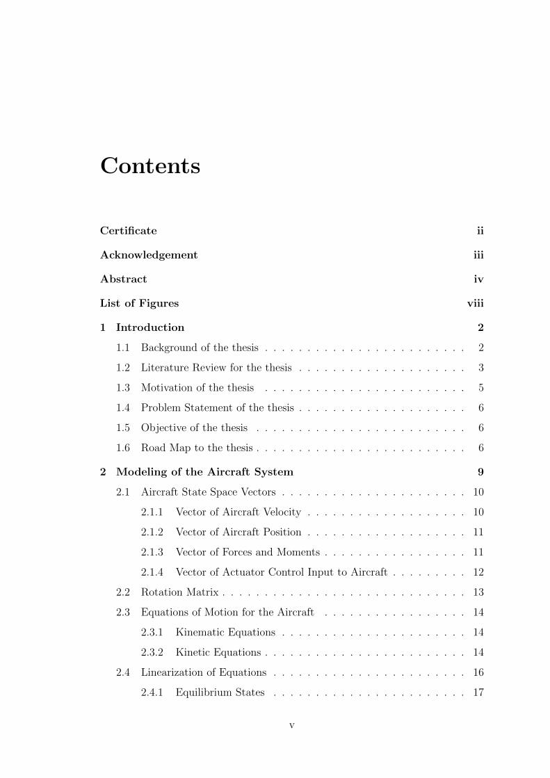
Contents

Certificate ii

Acknowledgement iii

Abstract iv

List of Figures viii

1 Introduction 2

1.1 Background of the thesis . . . . . . . . . . . . . . . . . . . . . . . . 2

1.2 Literature Review for the thesis . . . . . . . . . . . . . . . . . . . . 3

1.3 Motivation of the thesis . . . . . . . . . . . . . . . . . . . . . . . . 5

1.4 Problem Statement of the thesis . . . . . . . . . . . . . . . . . . . . 6

1.5 Objective of the thesis . . . . . . . . . . . . . . . . . . . . . . . . . 6

1.6 Road Map to the thesis . . . . . . . . . . . . . . . . . . . . . . . . . 6

2 Modeling of the Aircraft System 9

2.1 Aircraft State Space Vectors . . . . . . . . . . . . . . . . . . . . . . 10

2.1.1 Vector of Aircraft Velocity . . . . . . . . . . . . . . . . . . . 10

2.1.2 Vector of Aircraft Position . . . . . . . . . . . . . . . . . . . 11

2.1.3 Vector of Forces and Moments . . . . . . . . . . . . . . . . . 11

2.1.4 Vector of Actuator Control Input to Aircraft . . . . . . . . . 12

2.2 Rotation Matrix . . . . . . . . . . . . . . . . . . . . . . . . . . . . . 13

2.3 Equations of Motion for the Aircraft . . . . . . . . . . . . . . . . . 14

2.3.1 Kinematic Equations . . . . . . . . . . . . . . . . . . . . . . 14

2.3.2 Kinetic Equations . . . . . . . . . . . . . . . . . . . . . . . . 14

2.4 Linearization of Equations . . . . . . . . . . . . . . . . . . . . . . . 16

2.4.1 Equilibrium States . . . . . . . . . . . . . . . . . . . . . . . 17

v

2.4.2 Perturbed Equations . . . . . . . . . . . . . . . . . . . . . . 17

2.5 Aerodynamic Moments and Forces . . . . . . . . . . . . . . . . . . 18

2.5.1 Longitudinal Mode . . . . . . . . . . . . . . . . . . . . . . . 18

2.5.2 Lateral Mode . . . . . . . . . . . . . . . . . . . . . . . . . . 18

2.6 Decoupled State Space Model . . . . . . . . . . . . . . . . . . . . . 19

2.6.1 State Space Model for Longitudinal Mode . . . . . . . . . . 19

2.6.2 State Space Model for Lateral Mode . . . . . . . . . . . . . 20

2.7 State Space Model for the Aircraft B-767 . . . . . . . . . . . . . . . 22

2.7.1 Longitude Mode . . . . . . . . . . . . . . . . . . . . . . . . . 22

2.7.2 Lateral Mode . . . . . . . . . . . . . . . . . . . . . . . . . . 24

3 Model Predictive Control Strategy for the Aircraft System 28

3.1 Advantage of Model Predictive Control . . . . . . . . . . . . . . . . 29

3.2 Model Predictive Control Strategy . . . . . . . . . . . . . . . . . . 29

3.3 Continuous Time Model Predictive Control Strategy . . . . . . . . 31

3.4 Leguerre Function . . . . . . . . . . . . . . . . . . . . . . . . . . . . 32

3.5 Predicted Plant Model . . . . . . . . . . . . . . . . . . . . . . . . . 33

3.6 Predictive Control Strategy . . . . . . . . . . . . . . . . . . . . . . 35

3.7 Model predictive control for the aircraft . . . . . . . . . . . . . . . . 36

4 Modeling of the Aircraft Engine 41

4.1 Principle of Aircraft Propulsion . . . . . . . . . . . . . . . . . . . . 41

4.2 System Description . . . . . . . . . . . . . . . . . . . . . . . . . . . 42

4.3 System Parameter . . . . . . . . . . . . . . . . . . . . . . . . . . . . 43

4.4 System Dynamics . . . . . . . . . . . . . . . . . . . . . . . . . . . . 43

5 Fault Detection and Isolation Strategy 48

5.1 Fault Detection and Isolation Logic . . . . . . . . . . . . . . . . . . 48

5.2 Identification of Sensor Fault . . . . . . . . . . . . . . . . . . . . . . 50

5.3 Fault Identification and Isolation for the Modeled Aircraft Engine . 52

5.3.1 No Sensor Fault . . . . . . . . . . . . . . . . . . . . . . . . . 53

5.3.2 Fault in the Core Shaft Speed Measurement Sensor . . . . . 55

5.3.3 Fault in the Fan Shaft Speed Measurement Sensor . . . . . . 58

6 Conclusion and Scope for Future Work 61

6.1 Conclusion . . . . . . . . . . . . . . . . . . . . . . . . . . . . . . . . 61

6.2 Scope for Future Work . . . . . . . . . . . . . . . . . . . . . . . . . 62

Bibliography 63

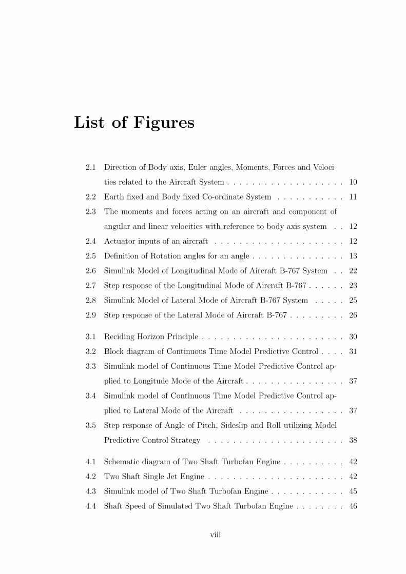
List of Figures

2.1 Direction of Body axis, Euler angles, Moments, Forces and Veloci-

ties related to the Aircraft System . . . . . . . . . . . . . . . . . . . 10

2.2 Earth fixed and Body fixed Co-ordinate System . . . . . . . . . . . 11

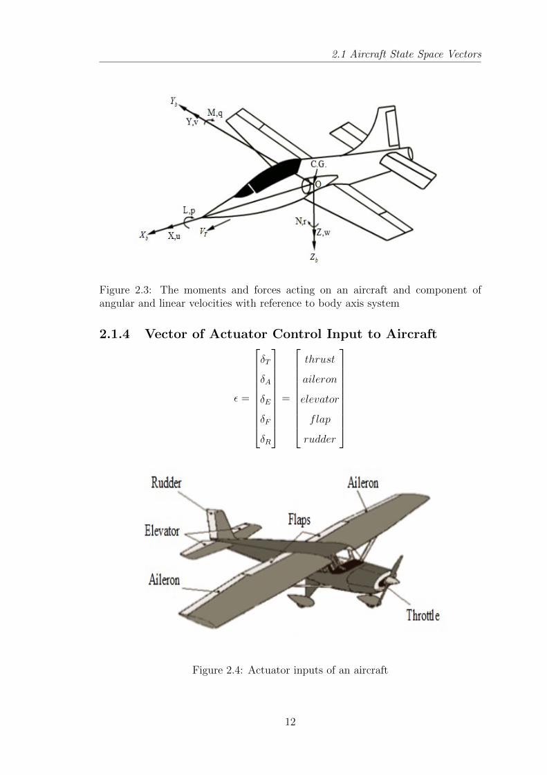
2.3 The moments and forces acting on an aircraft and component of

angular and linear velocities with reference to body axis system . . 12

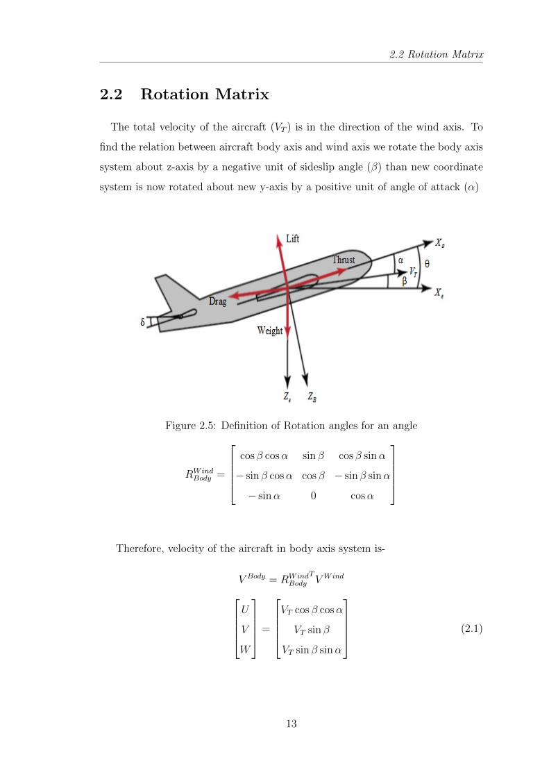
2.4 Actuator inputs of an aircraft . . . . . . . . . . . . . . . . . . . . . 12

2.5 Definition of Rotation angles for an angle . . . . . . . . . . . . . . . 13

2.6 Simulink Model of Longitudinal Mode of Aircraft B-767 System . . 22

2.7 Step response of the Longitudinal Mode of Aircraft B-767 . . . . . . 23

2.8 Simulink Model of Lateral Mode of Aircraft B-767 System . . . . . 25

2.9 Step response of the Lateral Mode of Aircraft B-767 . . . . . . . . . 26

3.1 Reciding Horizon Principle . . . . . . . . . . . . . . . . . . . . . . . 30

3.2 Block diagram of Continuous Time Model Predictive Control . . . . 31

3.3 Simulink model of Continuous Time Model Predictive Control ap-

plied to Longitude Mode of the Aircraft . . . . . . . . . . . . . . . . 37

3.4 Simulink model of Continuous Time Model Predictive Control ap-

plied to Lateral Mode of the Aircraft . . . . . . . . . . . . . . . . . 37

3.5 Step response of Angle of Pitch, Sideslip and Roll utilizing Model

Predictive Control Strategy . . . . . . . . . . . . . . . . . . . . . . 38

4.1 Schematic diagram of Two Shaft Turbofan Engine . . . . . . . . . . 42

4.2 Two Shaft Single Jet Engine . . . . . . . . . . . . . . . . . . . . . . 42

4.3 Simulink model of Two Shaft Turbofan Engine . . . . . . . . . . . . 45

4.4 Shaft Speed of Simulated Two Shaft Turbofan Engine . . . . . . . . 46

viii

5.1 Block Diagram of the Fault Detection and Isolation Strategy . . . . 49

5.2 Simulink Model of the Fault Detection and Isolation Strategy ap-

plied to the Aircraft Engine . . . . . . . . . . . . . . . . . . . . . . 52

5.3 Estimated Output of Kalman Filter 1 . . . . . . . . . . . . . . . . . 53








5.11 Residual Vector for all Kalman Filters . . . . . . . . . . . . . . . . 57

5.12 WSSR for all the Kalman Filter . . . . . . . . . . . . . . . . . . . . 57

5.13 Residual Vector for all Kalman Filters when Faulty Fan Shaft Speed

Measurement Sensor . . . . . . . . . . . . . . . . . . . . . . . . . . 58

5.14 WSSR for all the Kalman Filter when Faulty Fan Shaft Speed Mea-

surement Sensor . . . . . . . . . . . . . . . . . . . . . . . . . . . . . 59

Introduction

Chapter 1

Introduction

Nowadays, the accident in aircraft increasing and according to NTSB data [1],

aircraft system malfunctions were related to 52% of the accident whereas propul-

sion system malfunctions cause 36% of the accident. The increasing complexity of

aerospace system such as jet engines and cost reduction measure, which affected

aircraft and engine maintenance operators are increasingly demanding more in-

telligence, automation capabilities and functionalities for diagnosis and system

malfunctions. Therefore, it is important to identify the occurrence of faulty con-

ditions in the aircraft and to isolate these faults. By enabling the fault diagnosis

strategy for aircraft engine can altogether enhance the flight safety.

1.1 Background of the thesis

As 52% of the flight accident are related to aircraft system malfunction so it is

significant to understand the basic model of an aircraft, which includes aircraft

dynamics, forces and moments, wind turbulence etc. The aircraft model can eas-

ily be understood by understanding the dynamic equations of motion of aircraft.

Since the aircraft model is highly nonlinear, therefore it is also required to convert

it in a linear model.

A flight accident can cost the human lives as well as money, therefore it is

necessary to design a controller, which achieves the specific performances of the

aircraft model. A name suggest, model predictive control strategy is a control

2

1.2 Literature Review for the thesis

strategy based on models,which can easily handle basic changes,for example, fail-

ure actuator and sensor and system parameters changes by adjusting the control

strategy on a specimen by test premise. Principle of receding horizon, is an impor-

tant feature of model predictive control strategy, which optimized current state

by considering the future state into account.

A flight accident can also occur due to propulsion system malfunction, which

covers 36% of the flight accident. A fault diagnosis scheme for aircraft engine sig-

nifies the fault identification and its seclusion. Fault identification and isolation

scheme play an essential part in upgrading the safety, reliability and minimizing

the working expensive of propulsion system of the aircraft. Nonetheless, accom-

plishing the fault identification and its seclusion with high reliability is a testing

issue, That is why different methodology have been presented in the aircraft con-

trol literature.

Some of the approaches used in fault detection and isolation scheme are Kalman

filtering, neural networks and hybrid diagnosis. Numerous current fault identify

and seclusion scheme are taking into account the suspicion that the system shows

linear nature in the surrounding of the operating points at the steady state. Ac-

cordingly, diagnostic schemes based on linearization are generally utilized. Since

the dynamics of the aircraft engine are exceedingly nonlinear, therefore traditional

linear model Kalman filter method, subjected to linear uncertainties is used.


The basic model of aircraft is easily understood by mathematical modelling of

the aircraft. M.V. Cook discuss about a linear system approach to aircraft stability

and control in his book Flight Dynamic Principles [5]. D. Caughey gives the in-

troduction to the aircraft modelling, stability and control [3]. He presents various

views on implication of aircraft symmetry, aerodynamic control, force and mo-

ment coefficient of aircraft and its static stability and control. T.I. Fossen present

3


an approach to mathematical modelling of aircraft and satellite [2]. J. Blakelock

discuss the automatic control of aircraft and comment on its stability [4].

Model predictive control has grown significantly throughout the most recent

two decades, both inside the research control group and in the industry. A gen-

eral disturbance model which suit unmeasured noise entering through the process

data, output or state is presented by K.R. Muske and T.A. Badgwell while A.

Bemporad, M. Morari and J. Maciejowski presents the explicit state feedback

solution to linear quadratic optimal control issue subjected to the state and in-

put constraints [7–9]. E.F. Camacho and C. Bordons focuses on implementation

issues for model predictive control and intended to present easy way of implement-

ing them in the industry [10]. A. Suardi and G. constantinides present a system

on a chip model predictive control, implemented on a field programmable gate

array [6]. M. Kale and A. Chipperfield present formulation of model predictive

control scheme implemented to a realistic nonlinear model of an aircraft [24].

Aircraft engines constitutes a complex system, obliging satisfatory observation

to guarantee flight safety and timely maintenance. With a specific end goal to

observing the aircract engine Y. Guan, J. Warng and T. Lee present a technique

of digital simulation for the aircraft turbofan engine control system called method

of spare parts [13]. H. Spang and H. Brown review the basics of controlling an en-

gine while satisfying numerous constraints [14]. P. Shankar and M. Siddiqi discuss

a nonlinear mathematical model of two shaft turbofan engine utilizing the first

principal [15]. A. Alexiou and K. Mathioudakis talk about the demonstrating of a

turbine engine utilizing a general purpose simulation tool EcosimPro [21]. On the

other hand, F. Correa, A. Oliviera and R. Bosa gives an idea about turbo shaft

nonlinear dynamical model and its control system used for electric power genera-

tion [22]. C. Kong and J. Park give a overview on a turbine engine for unmanned

aerial vehicle [23].

4

1.3 Motivation of the thesis

Lately, impressive research endeavors has been given to fault identification of

nonlinear systems. For this reason, different methodology have been presents in

the literature. W. Xue, Y. Guo and X. Zhang presented Kalman filter techniques

for the detection of the fault in sensor and actuators [19]. W. Merrill and W.

Bruton also utilized a bank of Kalman filters for identification of sensor faulr and

its seclusion of an aircraft engine [25]. M. Seok and B. Jung works on techniques of

speed and surge control of an unmanned aircraft vehical with turbojet engine [26].

X. Zhang, L. Tang and J. Decastro present a fault identification and seclusion

scheme by using nonlinear adaptation estimator methodolgy for aircraft engines

[1]. F. Lu and J. Huang present a model based approach for optimal estimation

of engine performances [27]. A Kalman filter was applied by C. Hajiyev and F.

Caliskan [28]. This method pertains to the flaws that influences the mean of

innovation sequence of the Kalman filter . A sensor flaw could be identified and

secluded if it changes the innovation sequence mean value. A Robust Kalman

Filter was utilized to recognize the actuator and sensor flaw. But this technique

could not utilize to separate which actuator is defective.

1.3 Motivation of the thesis

The issues of reliability, affordability, safety and system integrity have turn out

to be progressively imperative as the mishap in the aircraft is increasing because

of the system malfunctions. Therefore, it is important to identify the occurrence

of faulty conditions in the aircraft and to isolate these faults. By enabling the fault

diagnosis strategy for aircraft engine can remarkably enhance the flight safety.

Model predictive control can consider hard constraints on the system. It can

easily be tuned and can also be applied to MIMO systems, which is advantage of

the model predictive controller over PID, LQ and H∞ controller.

State estimates can provide valuable information about important variables

of the physical process. Controller can use this valuable information about the

5

1.6 Road Map to the thesis

process to control it more accurately. In other words, System estimators can be a

practical or economical alternative to real measurement. The Kalman filter is the

most important algorithm for the state estimation.

1.4 Problem Statement of the thesis

The increasing complexity of aerospace system, aircraft and engine maintenance

operators are increasingly demanding more intelligence, automation capabilities

and functionalities for diagnosis and system malfunctions. Increasing the func-

tionality for fault diagnosis, system and propulsion malfunctions is necessary for

flight safety.

1.5 Objective of the thesis

• To design an efficient model of aircraft in Matlab and simulate the designed

model in Simulink and to comment the different stability mode of the aircraft

model.

• To design an efficient control law to achieve specific performance of the

aircraft mode. The specific performance is to achieve the set point of input

while keeping the output in a particular limit.

• To design an efficient model of a two shaft engine turbine engine in Simulink

• To design an efficient algorithm for the aircraft engine to detect its faults

and to isolate these faults.


The road map to the thesis is as follows:

• Chapter 2: The study of dynamics (kinematics and kinetics) of an aircraft

and an open loop study of aircraft with some proper modeling assumption

are being dealt in this chapter.

6


• Chapter 3: A model predictive controller has been proposed for the con-

trol of pitch angle, sideslip angle and roll angle of the aircraft, in which

continuous time model predictive control strategy is developed.

• Chapter 4: Deals with study of dynamics of fan shaft and core shaft of a

two shaft gas turbine engine.

• Chapter 5: A fault detection and isolation strategy has been present for

detection of speed sensor fault in a two spool gas turbine engine. In fault

detection and isolation strategy, a bank of Kalman filter is apply for identi-

fication and seclusion of faults.

• Chapter 6: Conclusion of the thesis along with some future suggestions are

presented in this very chapter

7

Modeling of the Aircraft System

Chapter 2

Modeling of the Aircraft System

For any type of aircraft the first step in obtaining the accurate mathematical

model is to determine stability and control derivatives. These derivatives will im-

pact the flying characteristics and will be used to size control surface, design flight

control system and program devise such as simulator. Three approaches can be

taken towards completing this goal.

The first and easiest method requires the knowledge of the geometry and iner-

tial properties of the aircraft and employ simple calculation to obtain the deriva-

tives within reasonable accuracy. The second method involves the use of wind

tunnels. However, the results will have to be refined after several scale, inter-

ference and dynamic effects are taken into account. This method is much more

complicated than the previous one, but usually more accurate. The final approach

which is the most time consuming and costly but with the most promise and preci-

sion in flight testing. Dynamic flight test data is used through techniques such as

parameter estimation to accurately estimate the stability and control derivatives.

Of course limitation in availability of data and noisy measurements can cause se-

rious problems in the successful resolution of all the derivatives of interest.

In the design of the mathematical model of the aircraft in Matlab / Simulink,

we consider only the first method which uses the knowledge of the geometry and

inertial properties of the aircraft. Using the laws of kinetic and kinematic the

equation of motion of the aircraft is derived and linearized about longitudinal

9

2.1 Aircraft State Space Vectors

equilibrium.

Figure 2.1: Direction of Body axis, Euler angles, Moments, Forces and Velocitiesrelated to the Aircraft System

The aircraft model can easily be understood by understanding the equations

that govern the motion of the aircraft. These equations governing the motion of

aircraft can be derived from the basic laws of kinetic and kinematic. The equations

governing the aircraft motion are linearized (since nonlinear) utilizing the theory

of perturbation and finally gives the state space models for longitudinal motion

and lateral motion.


To derive the equations of motion, first we define aircraft state space vectors as

2.1.1 Vector of Aircraft Velocity

ν =

U

V

W

P

Q

R

=

velocity in forward direction

velocity in transverse direction

velocity in verticle direction

rate of roll motion

rate of pitch motion

rate of yaw motion

10


where, VT =√U2 + V 2 +W 2 is the velocity of the aircraft.

2.1.2 Vector of Aircraft Position

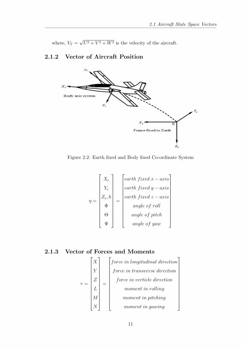
Figure 2.2: Earth fixed and Body fixed Co-ordinate System

η =

Xe

Ye

Ze, h

Φ

Θ

Ψ

=

earth fixed x− axis

earth fixed y − axis

earth fixed z − axis

angle of roll

angle of pitch

angle of yaw

2.1.3 Vector of Forces and Moments

τ =

X

Y

Z

L

M

N

=

force in longitudinal direction

force in transverse direction

force in verticle direction

moment in rolling

moment in pitching

moment in yawing

11


Figure 2.3: The moments and forces acting on an aircraft and component ofangular and linear velocities with reference to body axis system

2.1.4 Vector of Actuator Control Input to Aircraft

ε =

δT

δA

δE

δF

δR

=

thrust

aileron

elevator

flap

rudder

Figure 2.4: Actuator inputs of an aircraft

12

2.2 Rotation Matrix

2.2 Rotation Matrix

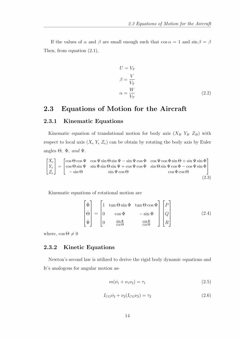
The total velocity of the aircraft (VT ) is in the direction of the wind axis. To

find the relation between aircraft body axis and wind axis we rotate the body axis

system about z-axis by a negative unit of sideslip angle (β) than new coordinate

system is now rotated about new y-axis by a positive unit of angle of attack (α)

Figure 2.5: Definition of Rotation angles for an angle

RWindBody =

cos β cosα sin β cos β sinα

− sin β cosα cos β − sin β sinα

− sinα 0 cosα

Therefore, velocity of the aircraft in body axis system is-

V Body = RWindBody

TV Wind

U

V

W

=

VT cos β cosα

VT sin β

VT sin β sinα

(2.1)

13

2.3 Equations of Motion for the Aircraft

If the values of α and β are small enough such that cosα = 1 and sin β = β

Then, from equation (2.1),

U = VT

β =V

VT

α =W

VT(2.2)


2.3.1 Kinematic Equations

Kinematic equation of translational motion for body axis (XB YB ZB) with

respect to local axis (Xe Ye Ze) can be obtain by rotating the body axis by Euler

angles Θ, Φ, and Ψ.Xe

YeZe

=

cos Θ cos Ψ cos Ψ sin Θ sin Ψ− sin Ψ cos Φ cos Ψ cos Φ sin Θ + sin Ψ sin Φcos Θ sin Ψ sin Φ sin Θ sin Ψ + cos Ψ cos Φ sin Θ sin Ψ cos Φ− cos Ψ sin Φ− sin Θ sin Ψ cos Θ cos Φ cos Θ

(2.3)

Kinematic equations of rotational motion areΦ

Θ

Ψ

=

1 tan Θ sin Φ tan Θ cos Φ

0 cos Φ − sin Φ

0 sin Φcos Θ

cos Φcos Θ

P

Q

R

(2.4)

where, cos Θ 6= 0

2.3.2 Kinetic Equations

Newton’s second law is utilized to derive the rigid body dynamic equations and

It’s analogous for angular motion as-

m(ν1 + ν1ν2) = τ1 (2.5)

ICGν2 + ν2(ICGν2) = τ2 (2.6)

14


where,

ν1 =

U

V

W

ν2 =

P

Q

R

τ1 =

X

Y

Z

τ2 =

L

M

N

Remark- It is assume that the coordinate system is located in the center of gravity

point of the aircraft therefore, for symmetric plane Ixy = Iyz = 0.

Hence resulting model can be written as-

MRB ν + CRB(ν)ν = τRB (2.7)

The affect of moments and forces on the aircraft come from the aerodynamics,

control forces and gravitational forces. The most important force in the flight is

gravity which act at the center of gravity point of the aircraft and parallel to local

Z-axis. Therefore, effect of the gravitational force on the aircraft is given as-

fG =

0

0

mg

In earth fixed (Xe Ye Ze) coordinate system

g(η) = −RXe Ye ZeXb Yb Zb

TfG

g(η) =

mg sin Θ

−mg sin Φ cos Θ

−mg cos Φ cos θ

0

0

0

15

2.4 Linearization of Equations

If a generalized vector τ includes aerodynamics and control forces, then the

moments and forces affecting the aircraft are-

τRB = −g(η) + τ (2.8)

Therefore, the kinetic equations of the aircraft can be written as from equation (2.6) and(2.7)

MRB ν + CRB(ν)ν + g(η) = τ (2.9)

In component form

m(U −RV +QW + g sin Θ) = X

m(V −WP + UR− g cos Θ sin Φ) = Y

m(W −QU + V P − g cos Θ cos Φ) = Z (2.10)

IXP − IXZ(R + PQ) + (IZ − IY )QR = L

IyQ− IXZ(P 2 −R2) + (IX − Iy)PR = M

IZR− IXZP − (IX − IY )PQ+ IXZRQ = N


According to Linear theory that the state can be written as sum of a nominal

value (generally constant) and a perturbation (derived from nominal value). The

equation (2.9) develop previously are nonlinear and coupled. These equations can

be simplify easily when the equilibrium condition is chosen corresponding to the

longitudinal equilibrium, in which the velocity and gravity vector are in the plane

of symmetry of vehicle.

16


Therefore,

U = u0 + u P = p (2.11)

V = v Q = q (2.12)

W = w R = r (2.13)

Θ = θ0 + θ Φ = φ (2.14)

The trim values of all lateral directional variables are zero because the initial

trim condition corresponds to the longitudinal equilibrium (v0 = p0 = r0 = φ0).

The value W0 is zero because we are using stability axis and the value q0 is zero

because we are restricting the equilibrium state to have no normal acceleration.

2.4.1 Equilibrium States

Equilibrium state can be written as-

mg0 sin θ0 = X0

−mg0 cos θ0 = Z0 (2.15)

M0 = L0 = Y0 = N0 = 0

2.4.2 Perturbed Equations

The perturbed equations can be obtained using equations (2.11), (2.12) and

(2.10). Neglect the higher order terms of the perturbed states. After perturbation

the moments and forces equations can be written as-

m(u+ g0 cos θ0θ) = δX

m(w − u0q + g0 sin θ0θ) = δZ

m(v + u0r − g0 cos θ0φ) = δY

IX p− IXZ r = δL

17

2.5 Aerodynamic Moments and Forces

IY q = δM (2.16)

Iz r − IXZ p = δN

θ = qφψ

=

1 tan θ0

0 1cos θ0

pr

; cos θ0 6= 0

2.5 Aerodynamic Moments and Forces

The perturbation in aerodynamic moments and forces are function of both state

variable and control inputs, which can be written as-

2.5.1 Longitudinal ModeδX

δZ

δM

=

Xu Xα Xq

Zu Zα Zq

Mu Mα Mq

u

α

q

+

Xu Xα Xq

Zu Zα Zq

Mu Mα Mq

u

α

q

+

Xδe XδT

Zδe ZδT

Mδe MδT

δeδT

For the conventional aircraft the following aerodynamics coefficient can be ne-

glected, i.e. Xu Xα Xq Zu Zq Xu Xα Xq are neglected. Hence, equation for

longitudinal mode of aerodynamic forces and moments reduces toδX

δZ

δM

=

0 0 0

0 Zα 0

0 Mα 0

u

α

q

+

Xu Xα 0

Zu Zα Zq

Mu Mα Mq

u

α

q

+

Xδe XδT

Zδe ZδT

Mδe MδT

δeδT

(2.17)

2.5.2 Lateral ModeδY

δL

δN

=

Yβ Yp Yr

Lβ Lp Lr

Nβ Np Nr

β

p

r

+

Yβ Yp Yr

Lβ Lp Lr

Nβ Np Nr

β

p

r

+

Yδa Yδr

Mδa Mδr

Nδa Nδr

δaδr

18

2.6 Decoupled State Space Model

For the conventional aircraft the following aerodynamics coefficient can be ne-

glected, i.e. Yβ Yp Yr Lβ Lp Lr Nβ Np Nr Yδa are neglected. Hence, equation for

longitudinal mode of aerodynamic forces and moments reduces toδY

δL

δN

=

Yβ Yp Yr

Lβ Lp Lr

Nβ Np Nr

β

p

r

+

0 Yδr

Mδa Mδr

Nδa Nδr

δaδr

(2.18)


A state space model for decoupled longitudinal mode as well as lateral mode

can be write by combining equations (2.2, 2.16, 2.17, 2.18).

2.6.1 State Space Model for Longitudinal Mode

From equations (2.2, 2.16, 2.17), we can write the equations governing the

motion of aircraft in longitudinal mode as-

u = Xuu+Xαα + g0cos θ0θ +Xδeδe +XδT δT

(1− Zα)α = Zuu+ Zαα + (Zq + u0)q − g0sin θ0θ + Zδeδe + ZδT δT

q = Muu+Mαα +Mαα +Mqq +Mδeδe +MδT δT

θ = q (2.19)

If we introduce longitudinal state vector X = [u w q θ]′ and control vector

ε = [δe δT ]′ Then equation (2.19) is equivalent to first order state space model

InX = AnX +Bnε

19


where,

An =

Xu Xα 0 g0 cos θ0

Zu Zα (Zq + u0) g0 sin θ0

Mu Mα Mq 0

0 0 1 0

Bn =

Xδe XδT

Zδe ZδT

Mδe MδT

0 0

In =

1 0 0 0

0 1− Zα 0 0

0 −Mα 1 0

0 0 0 1

I−1n =

1 0 0 0

0 11−Zα 0 0

0 Mα

1−Zα 1 0

0 0 0 1

Since aircraft mass factor (µ) is usually large (approximately 100), Therefore it

is usual to neglect Zα with respect to unity and Zq with respect to u0. By pre-

multiplying I−1n , the state space model of longitudinal mode takes the standard

form as

X = AX +Bε (2.20)

where,

A =

Xu Xα 0 −g0 cos θ0

Zu Zα u0 −g0 sin θ0

Mu +MαZu Mα +MαZα Mq +Mαu0 −Mαg0 sin θ0

0 0 1 0

B =

Xδe XδT

Zδe ZδT

Mδe +MαZδe MδT +MαZδT

0 0

2.6.2 State Space Model for Lateral Mode

From equations (2.2, 2.16, 2.18), we can write the lateral mode of equations of

motion as -

β = Yββ + Ypp+ (Yr + u0)r − g0cos θ0φ+ Yδaδa + Yδrδr

20


p = Lpp+ Lββ + Lrr +IXZIX

r + Lδrδr + Lδaδa

r = Npp+Nββ +Nrr +IXZIX

p+Nδrδr +Nδaδa (2.21)φψ

=

1 tan θ0

0 1cos θ0

pr

; cos θ0 6= 0

If we introduce lateral state vector X = [β p φ r]′ and control vector ε = [δa δr]′

Then equation (2.21) is equivalent to first order state space model

InX = AnX +Bnε

where,

An =

Yβ Yp g0 cos θ0 Yr − u0

Lβ Lp 0 Lr

0 1 0 0

Nβ Np 0 Nr

Bn =

0 Yδr

Lδa Lδr

0 0

Nδa Nδr

In =

1 0 0 0

0 1 0 − IXZIX

0 0 1 0

0 − IXZIZ

0 1

For most of the aircraft, the ratio IXZ

IXand IXZ

IZare quite small so we can neglect

these ratio with respect to unity. Therefore, the state space model of the lateral

mode takes the standard form as

X = AX +Bε (2.22)

where,

A =

Yβ Yp g0 cos θ0 Yr − u0

Lβ Lp 0 Lr

0 1 0 0

Nβ Np 0 Nr

B =

0 Yδr

Lδa Lδr

0 0

Nδa Nδr

21

2.7 State Space Model for the Aircraft B-767


2.7.1 Longitude Mode

Given, equilibrium point:

V elocity VT = 890 ft/s Altitude h = 35000 ft

Mass m = 184000 lbs Mach No. M = 0.8

If X = [u w q θ]′ and ε = [δe δT ]′ are longitudinal state and control vector

respectively then, state equation is-

X = AX +Bε

where,

A =

−0.0168 0.1121 0.0003 −0.5608

−0.0164 −0.7771 0.9945 0.0015

−0.0417 −3.6595 −0.9544 0

0 0 1 0

; B =

−0.0243 0.0519

−0.0634 −0.0005

−3.6942 0.0243

0 0

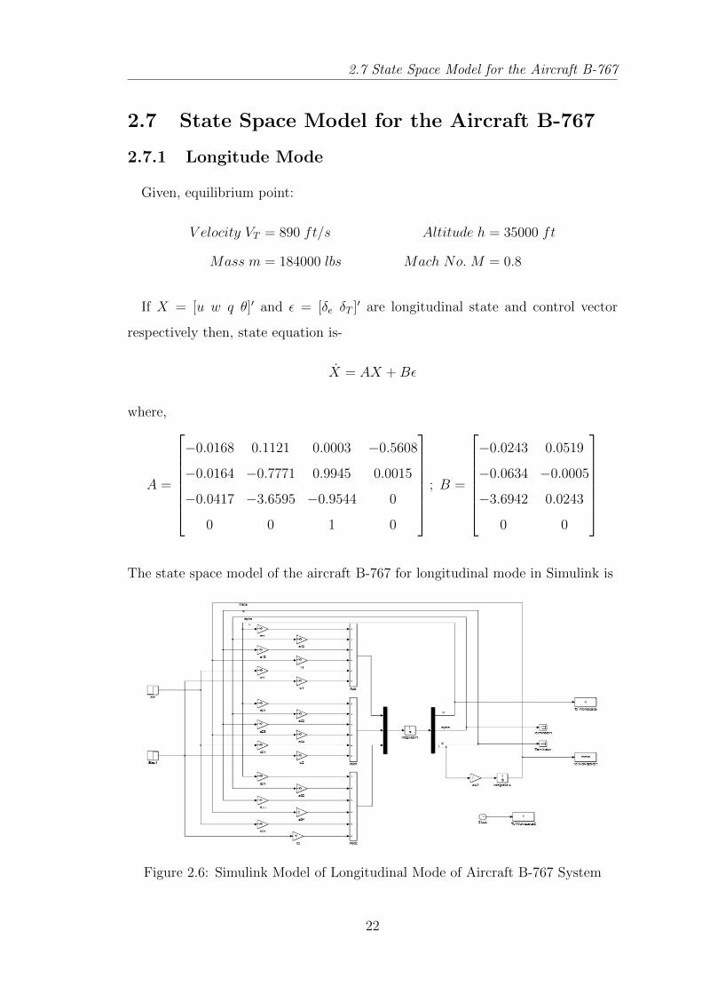
The state space model of the aircraft B-767 for longitudinal mode in Simulink is

Figure 2.6: Simulink Model of Longitudinal Mode of Aircraft B-767 System

22


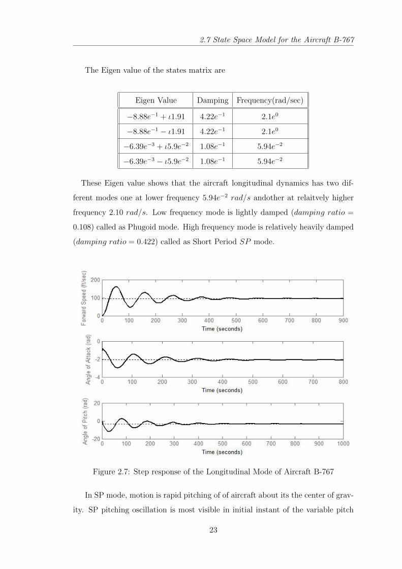
The Eigen value of the states matrix are

Eigen Value Damping Frequency(rad/sec)

−8.88e−1 + ι1.91 4.22e−1 2.1e0

−8.88e−1 − ι1.91 4.22e−1 2.1e0

−6.39e−3 + ι5.9e−2 1.08e−1 5.94e−2

−6.39e−3 − ι5.9e−2 1.08e−1 5.94e−2

These Eigen value shows that the aircraft longitudinal dynamics has two dif-

ferent modes one at lower frequency 5.94e−2 rad/s andother at relaitvely higher

frequency 2.10 rad/s. Low frequency mode is lightly damped (damping ratio =

0.108) called as Phugoid mode. High frequency mode is relatively heavily damped

(damping ratio = 0.422) called as Short Period SP mode.

Figure 2.7: Step response of the Longitudinal Mode of Aircraft B-767

In SP mode, motion is rapid pitching of of aircraft about its the center of grav-

ity. SP pitching oscillation is most visible in initial instant of the variable pitch

23


rate and angle of attack. SP mode is so short that the speed and pitch angle do not

have time to damp, that is why the oscillations are the variations in angle of attack.

Phugoid mode describes the long duration translatory motion of center of grav-

ity point of the vehicle. Phugoid mode can be excited by an elevator singlet result-

ing in a pitch increase with no change in trim condition from the cruise condition.

In Phugoid mode, the angle of attack remain nearly constant but varying the pitch

caused by a repeated exchange of airspeed and altitude.

2.7.2 Lateral Mode

Given, equilibrium point:

V elocity VT = 890 ft/s Altitude h = 35000 ft

Mass m = 184000 lbs Mach No. M = 0.8

If X = [v p φ r]′ and ε = [δa δr]′ are lateral state and control vector respectively

then, state equation is-

X = AX +Bε

where,

A =

−0.1245 0.0350 0.0414 −0.9962

−15.2138 −2.0587 0.0032 0.6458

0 1 0 0.0357

1.6447 −0.0447 −0.0022 −0.1416

; B =

−0.0049 0.0237

−4.0379 0.9613

0 0

−0.0568 −1.2168

The state space model of the aircraft B-767 for lateral mode in Simulink is

The Eigen value of the states matrix are

24


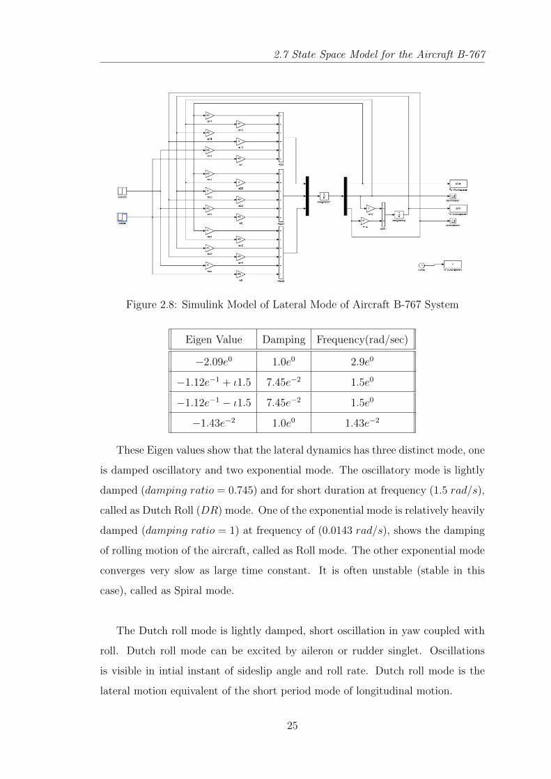
Figure 2.8: Simulink Model of Lateral Mode of Aircraft B-767 System

Eigen Value Damping Frequency(rad/sec)

−2.09e0 1.0e0 2.9e0

−1.12e−1 + ι1.5 7.45e−2 1.5e0

−1.12e−1 − ι1.5 7.45e−2 1.5e0

−1.43e−2 1.0e0 1.43e−2

These Eigen values show that the lateral dynamics has three distinct mode, one

is damped oscillatory and two exponential mode. The oscillatory mode is lightly

damped (damping ratio = 0.745) and for short duration at frequency (1.5 rad/s),

called as Dutch Roll (DR) mode. One of the exponential mode is relatively heavily

damped (damping ratio = 1) at frequency of (0.0143 rad/s), shows the damping

of rolling motion of the aircraft, called as Roll mode. The other exponential mode

converges very slow as large time constant. It is often unstable (stable in this

case), called as Spiral mode.

The Dutch roll mode is lightly damped, short oscillation in yaw coupled with

roll. Dutch roll mode can be excited by aileron or rudder singlet. Oscillations

is visible in intial instant of sideslip angle and roll rate. Dutch roll mode is the

lateral motion equivalent of the short period mode of longitudinal motion.

25


Figure 2.9: Step response of the Lateral Mode of Aircraft B-767

The Roll mode and Spiral mode are non-oscillatory mode. Roll mode consist

of purely rolling motion. It converges very quickly with heavily damping. Spiral

mode is complex coupled motion in roll, yaw and sideslip. It converges slow as

having large time constant. Spiral mode can be excited by a disturbance in sideslip

which follows in roll.

26

Model Predictive Control Strategy

for the Aircraft System

Chapter 3

Model Predictive ControlStrategy for the Aircraft System

Model predictive control strategy is controller scheme based on models, which

can easily handle basic changes,for example actuator and sensor failure and sys-

tem parameter changes by adjusting the control strategy on a specimen by test

premise. It designated an efficient control methods range, which utilize process

model explicitly to obtain the control sequence by optimizing an objective func-

tion.

The model predictive control strategy empowers a controller to be produced

which is ideal as for a specified quadratic execution record. In numerous pragmatic

control issues, it is direct to interpret the obliged performance objective useful into

an issue of optimizing a quadratic functional while applying the system constraints

on it.

The concept behind choosing the model predictive control is that, the model

predictive control has unmistakable point of interest over other kind of control

procedures for example, PID, Linear Quadratic and H∞. A PID controller is

effectively tuned however can just be connected to lower order SISO frameworks.

Direct Quadratic and H∞ controller can undoubtedly be connected to MIMO

frameworks however can’t deal with sign limitations in an sufficient way. Model

predictive control can consider hard requirements on the systems.

28

3.2 Model Predictive Control Strategy

3.1 Advantage of Model Predictive Control

Model predictive control has many advantages over the other controller some of

them are as follows

• It is utilized to control a great variety of procedures, from those with mod-

erately basic dynamics to more complex one, including systems with long

delay time or unstable or non-minimum phase one.

• The multivariable case can undoubtedly be managed.

• It presents feed forward control in a natural manner to compensate for mea-

surable unsettling influence.

• Its augmentation to the treatment of imperatives, is adroitly basic and can

be methodicallly included amid the outline process.

• It is a completely open approach in view of certain essential standards which

takes into account future augmentations.


Model predictive control is is a way to deal with controller outline that includes

online enhancement count. The improvement issue makes note of framework flow,

imperatives and control objective. The customary model predictive control re-

quires the arrangement of an open circle ideal control issue, in which choice vari-

able is an arrangement of control activities at every example time. Current control

activity is situated equivalent to the first term of the ideal control arrangement. A

key feature to model predictive control is the receding horizon principle, in which

current state is optimized by considering the future state into account.

The future outputs y(k+i|k) is predicted for a specific horizon. These predicted

output depends on the past input and outputs and future control signal u(k+ i|k).

29


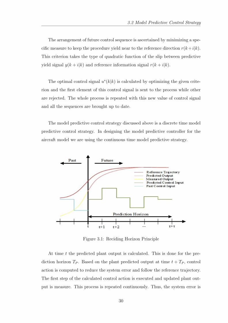
The arrangement of future control sequence is ascertained by minimizing a spe-

cific measure to keep the procedure yield near to the reference direction r(k+ i|k).

This criterion takes the type of quadratic function of the slip between predictive

yield signal y(k + i|k) and reference information signal r(k + i|k).

The optimal control signal u∗(k|k) is calculated by optimizing the given crite-

rion and the first element of this control signal is sent to the process while other

are rejected. The whole process is repeated with this new value of control signal

and all the sequences are brought up to date.

The model predictive control strategy discussed above is a discrete time model

predictive control strategy. In designing the model predictive controller for the

aircraft model we are using the continuous time model predictive strategy.

Figure 3.1: Reciding Horizon Principle

At time t the predicted plant output is calculated. This is done for the pre-

diction horizon TP . Based on the plant predicted output at time t + TP , control

action is computed to reduce the system error and follow the reference trajectory.

The first step of the calculated control action is executed and updated plant out-

put is measure. This process is repeated continuously. Thus, the system error is

30

3.3 Continuous Time Model Predictive Control Strategy

eliminated and output follows the input.

To take after the set point, the control sign need to join to a nonzero consis-

tent, i.e. identified with relentless state addition of the plant and extent of the set

point change. That is the reason, here, we are utilizing the first derivative of the

control sequence as opposed to utilizing it specifically.

3.3 Continuous Time Model Predictive Control

Strategy

In the recent years the interest in continuous - time MPC has grown. In the

work of Wang [13] it is shown that how to create continuous - time model pre-

dictive controller using the orthonormal basic functions. The big advantage of

this method is that it reduces the required computing power. In general, CTMPC

is more complicated than its discrete time counterpart. This is because in the

continuous time case, convolution is utilized to calculate the future plant behavior

instead of iteration.

Figure 3.2: Block diagram of Continuous Time Model Predictive Control

31

3.4 Leguerre Function

The design strategy presented here can be used as an substitute to classical

receding horizon control without the need to solve the matrix differential Ricatti

equation. The control trajectory is calculated using a pre-chosen set of orthonor-

mal basis functions. The first derivative of the control sequence can be approx-

imated within the prediction horizon using the orthonormal basis function [13].

Laguerre orthonormal basis function is used in this design. The novelty of this

approach lies in the way that the issue of finding the optimal control sequence is

changed over into one of the finding arrangement of coefficient for the Laguerre

model.

3.4 Leguerre Function

One set of Orthonormal basis function frequently used is Laguerre Function. It

satisfies the orthonormal property and defined as

lj(t) =√

2qeqt

j − 1!

dj−1

dtj−1[tj−1e−2qt] (3.1)

where, lj(t) is the Laguerre function. q ≥ 0, often called scaling factor and j =

1, 2.... The Laguerre function lj(t) is appealing to researcher because of having a

simpler form of Laplace transform as∫ ∞0

lj(t)e−stdt =

√2q

(s− q)j−1

(s+ q)j(3.2)

From equation (3.2), a differential equation can be derived which satisfied by

the Laguerre function. Let L(t) = [l1(t) l2(t)...lm(t)]′ and L(0) =√

2q[11...1]′

Then the differential equation satisfied by the Laguerre function

L(t) = AqL(t) (3.3)

where,

Aq =

−q 0 . . . 0 0

−2q −q . . . 0 0...

.... . .

......

−2q −2q . . . −2q −q

32

3.5 Predicted Plant Model

The equation (3.3) yield to a Laguerre function in form of exponential equation

of as

L(t) = eAqtL(0) (3.4)

For a linear time invariant stable closed loop system, the control sequence for the

change in set point, exponentially converges to a constant. Therefore, the control

sequence derivative u(t) converge to a value of zero, when it is assumed that the

closed loop system is stable within each moving horizon window tj ≤ t ≤ tj + TP .

It is seen that ∫ tj+TP

tj

u(t)2dt <∞ (3.5)

By applying the technique used by Wang[13]. The control sequence derivative

can be described by using a Laguerre function as

u(t) = L(t)Tκ (3.6)

where, κ is the vector coefficient of orthonormal function lj(t).


It is assume that input is not effecting the output directly. The plant (aircraft

system) to be controlled is a multivariable state space system with two input and

two output, described in the state space form as

xs(t) = Asxs(t) +Bsu(t)

y(t) = Csxs(t) (3.7)

Let us define an auxiliary variable H(t) = xs(t).

The state space system (equation 3.7) can now be written in an augmented form

xa(t) = Aaxa(t) +Bau(t)

33


y(t) = Caxa(t) (3.8)

where,

xa(t) =

H(t)

y(t)

Aa =

As 0

Cs 0

Ba =

Bs

0

Ca =[0 I

]

It is possible to track the output of the original system using a model predictive

control[13]. This only holds when there are no constraints acting on the system.

It is assumed that the state variable x(tj) is available at the current time tj.

Then at future time tj + τt; τt > 0, The predicted state variable x(tj + τt) is define

as

x(tj + τt) = eAaτtx(tj) +

∫ τt

0

eAa(τt−Γ)Bau(Γ)dΓ (3.9)

The control signal can be written as u(t) = [u1(t) u2(t)]. The jth control signal

uj(t) can be expressed as the orthonormal basis function.

uj(t) = Lj(t)Tκj (3.10)

Then the predicted future state at time tj + τt, x(tj + τt) is

x(tj + τt) = eAaτtx(tj) + φj(τt)Tκ (3.11)

where,

φj(τt)T =

∫ τt

0

eAa(τt−Γ)BjLj(Γ)TdΓ (3.12)

And the plant predicted output can be presented by

y(tj + τt) = Cax(tj + τt) (3.13)

34

3.6 Predictive Control Strategy

The convolution operation in equation (3.11) is the major problem in evaluat-

ing the prediction. The solution of the convolution integral φ(τ)T can be calculated

by satisfying the following linear algebraic equation.

Aqφ(τt)T − φ(τt)

TATq = −BL(τt)T + eAaτtBL(0)T (3.14)

Obtaining the matrix φ(τt)T as shown above, the prediction x(tj + τt) can be

determined and predicted output can be calculated.

3.6 Predictive Control Strategy

To compute the optimal control, a cost function has to be optimized. Let a

future set point r(tj + τt) = [r1(tj + τt) r2(tj + τ + t)] for 0 ≤ τt ≤ TP where TP is

the prediction horizon. The cost function can be defined as

I =

∫ TP

0

[r(tj + τt)− y(tj + τt)]TQ[r(tj + τt)− y(tj + τ)]dτt +

∫ TP

0

u(τt)TRu(τt)dτt

(3.15)

where Q and R are the symmetric weight matrices with Q ≥ 0, R ≥ 0.

when the set point is a constant signal, by subtracting r(tj) from variable

y(tj + τt), the augmented state vector takes the form

x(tj + τt) =

H(tj + τt)

e(tj + τt)

where, e(tj + τt) = y(tj + τt)− r(tj).

By choosing Q = CTC, in conjunction with the augmented model the cost

function can be written as

I =

∫ TP

0

[x(tj + τt)TQx(tj + τt) + u(τt)

TRu(τt)]dτt (3.16)

where, x(tj + τt) contains the error e(tj + τt) = y(tj + τt)− r(tj) instead of y(tj).

By exploiting the orthonormal properties of the Laguerre function the cost

function can be composed as

I =

∫ TP

0

[x(tj + τt)TQx(tj + τt)]dτt + κTRLκ (3.17)

35

3.7 Model predictive control for the aircraft

Putting the state variable from equation (3.11) in equation (3.17) and the

solving it. we get

I = [κ+ F−1Gx(tj)]TF [κ+ F−1Gx(tj)] + x(tj)

T

∫ TP

0

eATa τtQeAaτtdτtx(tj)

− x(tj)TGTF−1Gx(tj) (3.18)

where,

F =

∫ TP

o

φ(τt)TQφ(τt)dτt +RL

G =

∫ TP

o

φ(τt)QeAaτtdτ

The minimum of the cost function (equation 3.18) without hard constraints on

variable is given by the least square solution.

κ = −F−1Gx(tj) (3.19)

The derivation of the control input u(t) can now be computed from equations

(3.10) and (3.19) as

u(tj) = −Lj(τt)F−1Gx(tj) (3.20)

or

u(tj) = −kmpcx(tj)

where, kmpc = Lj(τt)F−1G is the model predictive controller gain matrix.

By integrating the equation (3.20) we will get our control law. Because of

the cost function (equation 3.18) is a quadratic function, it is easy to put hard

constraints on the states, outputs, and control variables of the system.


Before applying the model predictive control strategy to the aircraft model, the

aircraft system is stable but unable to achieve good transient performances to the

change in various inputs such as elevator,aileron and rudder, which is undesirable

see figure. For the aircraft system, not having good transient performances leads

to instability of the system.

36


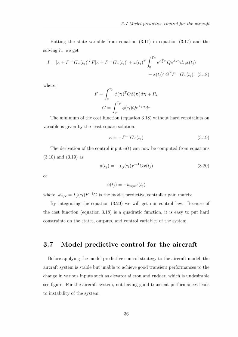
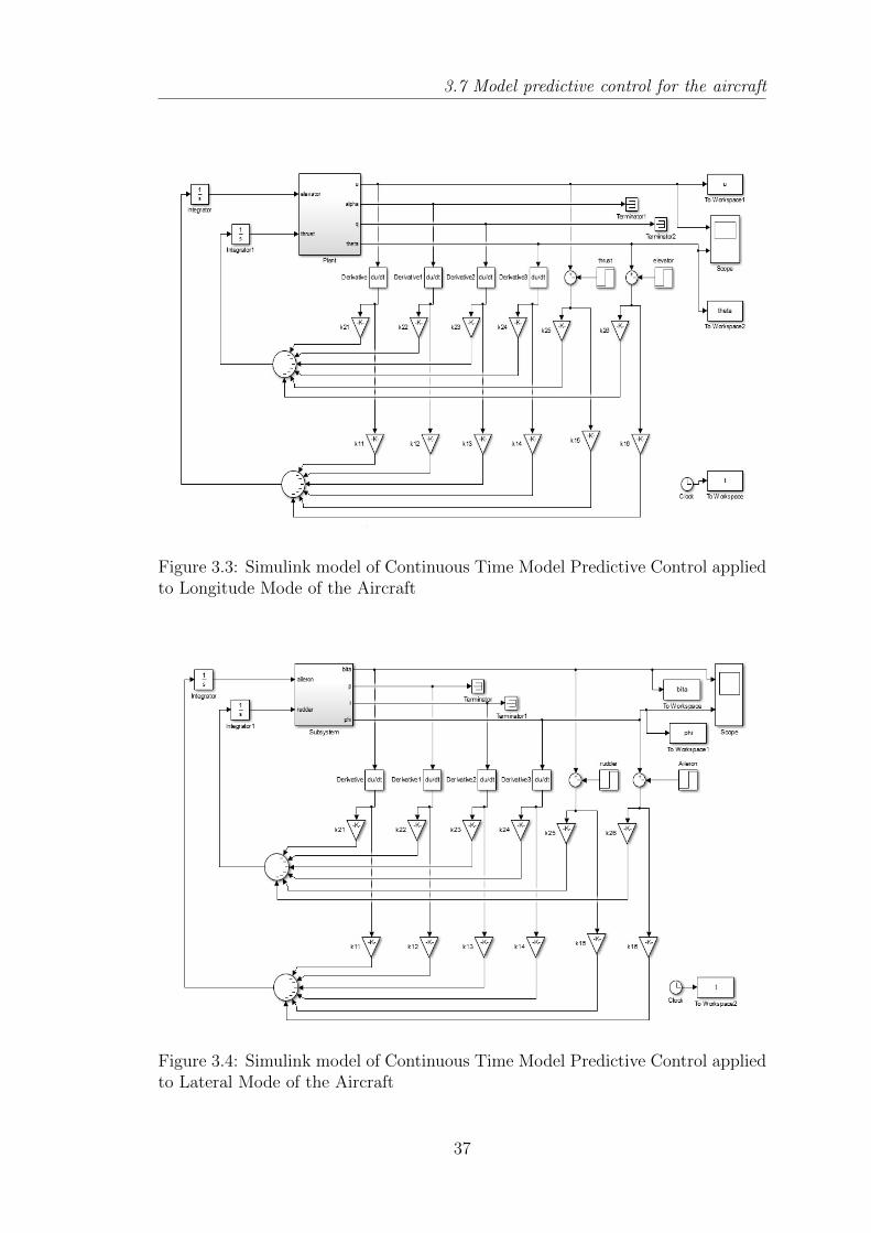
Figure 3.3: Simulink model of Continuous Time Model Predictive Control appliedto Longitude Mode of the Aircraft

Figure 3.4: Simulink model of Continuous Time Model Predictive Control appliedto Lateral Mode of the Aircraft

37


Above discussed model predictive control strategy is applied to the simulated

mathematical model of the aircraft Boeing-767. Simulation were pursuit utilizing

Matlab / Simulink to understand the effect of model predictive control strategy

on the aircraft system.

In the MPC design for the aircraft we are changing the input actuator as el-

evator, aileron and rudder and seeing the effect in the transient performances of

the pitch angle, anlge of sideslip and the angle of roll.

Figure 3.5: Step response of Angle of Pitch, Sideslip and Roll utilizing ModelPredictive Control Strategy

After applying the MPC to the aircraft control system, the poles of the overall

system shifted towards the left of the s-plane. Therefore, the stability of the sys-

tem is increased as well as the transient performances of the system now reduces

38


to small value as compared to the previous case.

Figure 3.5 shows the improved transient performance of the aircraft control

system. From figure, it is clear that the application of the MPC to the aircraft

control system is very helpful to achieve the desired performances and tracking

the references or the regulation of the system.

39

Modeling of an Aircraft Engine

Chapter 4

Modeling of the Aircraft Engine

An engine of an aircraft constitute a complex system, which obliging efficient

checking for guaranteed flight safety and time to time maintenance. In order

to monitoring the aircraft engine, a mathematical model of aircraft engine is to

be design in Matlab / Simulink. In designing the mathematical model of double

spool turbofan engine we focus on fuel flow rate, exhaust nozzle opening and spool

speeds, because of their interesting properties, resulted from theoretical and ex-

perimental studies.

Modern aircraft engines, mainly the fighter aircraft engines must have high

level of thrust, low transient response and maneuverability. For a higher level of

thrust, compressors pressure ratio and temperature of combustor must be high.

For high values of compressor pressure ratio, the compressor must be split in two

or more parts. A gas turbine is coupled with each compressor unit i.e. turbo-

compressor shaft or spools. In other words, To achieve high level of thrust and

high compressor ratio a simple engine is converted to a multi-shaft engine. Each

shaft rotates at different speed.

4.1 Principle of Aircraft Propulsion

Fundamental rule in a airplane motor is to quicken a mass of fluid in the heading

inverse to movement and along these lines moving the flying machine forward by

41

4.2 System Description

the push generated. The motor sucks air in at the front with a fan. A compressor

raises the weight of the air. The compressor is comprised of fans with numerous

edges and joined to a pole. The edges pack the air. The compacted air is then

showered with fuel and an electric sparkle lights the blend in the combustor. The

smoldering gasses grow and impact out through the spout, at the back of the

motor. As the planes of gas shoot in reverse, the motor and the air ship are push

forward.

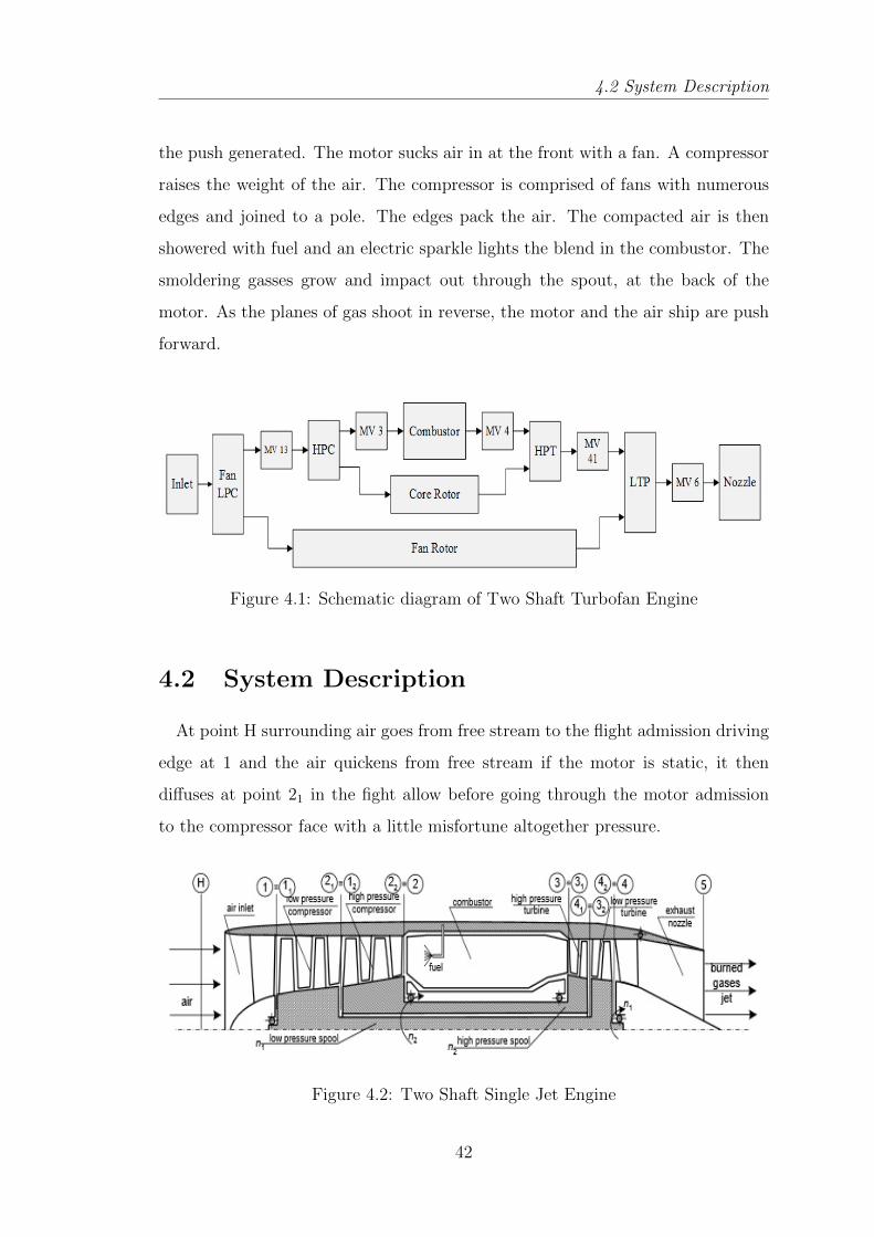
Figure 4.1: Schematic diagram of Two Shaft Turbofan Engine

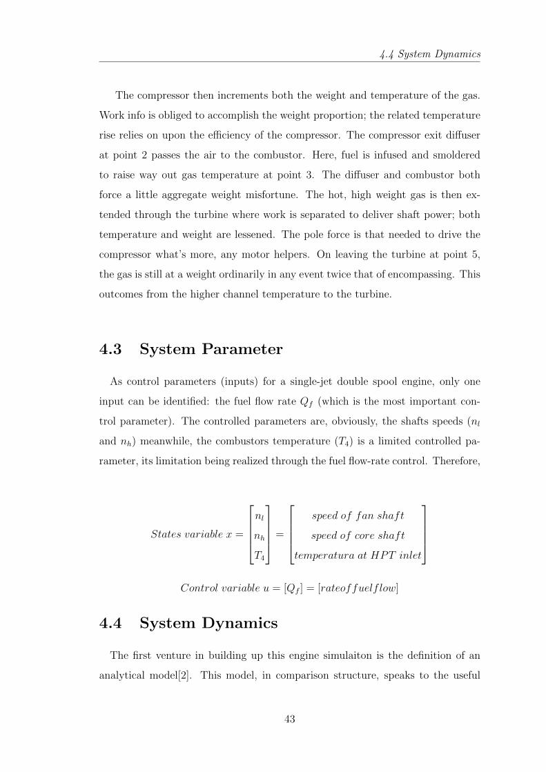
4.2 System Description

At point H surrounding air goes from free stream to the flight admission driving

edge at 1 and the air quickens from free stream if the motor is static, it then

diffuses at point 21 in the fight allow before going through the motor admission

to the compressor face with a little misfortune altogether pressure.

Figure 4.2: Two Shaft Single Jet Engine

42

4.4 System Dynamics

The compressor then increments both the weight and temperature of the gas.

Work info is obliged to accomplish the weight proportion; the related temperature

rise relies on upon the efficiency of the compressor. The compressor exit diffuser

at point 2 passes the air to the combustor. Here, fuel is infused and smoldered

to raise way out gas temperature at point 3. The diffuser and combustor both

force a little aggregate weight misfortune. The hot, high weight gas is then ex-

tended through the turbine where work is separated to deliver shaft power; both

temperature and weight are lessened. The pole force is that needed to drive the

compressor what’s more, any motor helpers. On leaving the turbine at point 5,

the gas is still at a weight ordinarily in any event twice that of encompassing. This

outcomes from the higher channel temperature to the turbine.

4.3 System Parameter

As control parameters (inputs) for a single-jet double spool engine, only one

input can be identified: the fuel flow rate Qf (which is the most important con-

trol parameter). The controlled parameters are, obviously, the shafts speeds (nl

and nh) meanwhile, the combustors temperature (T4) is a limited controlled pa-

rameter, its limitation being realized through the fuel flow-rate control. Therefore,

States variable x =

nl

nh

T4

=

speed of fan shaft

speed of core shaft

temperatura at HPT inlet

Control variable u = [Qf ] = [rateoffuelflow]

4.4 System Dynamics

The first venture in building up this engine simulaiton is the definition of an

analytical model[2]. This model, in comparison structure, speaks to the useful

43

4.4 System Dynamics

relations that exist between the engine variables, for example, weights, tempera-

tures, and gas flow rates. The engine model ought to be fit for precisely foreseeing

both the enduring state and element execution of the engine.

Shafts rate are straightforwardly connected with mass course through the mo-

tor and the push, which is the principle yield to be controlled by the impetus

control system.If nl and nh are the fan shaft speed and center shaft speed sepa-

rately then as indicated by Newton’s law for pivoting masses connected to each

shaft.

nl = fl(nl, nh, Qf , T4)

nh = fh(nl, nh, Qf , T4) (4.1)

where fl and fh are the net torque conveyed by the low pressure turbine and

high pressure turbine respectively after normalizing by mass moment of inertia of

shaft congregations.

Because of complicated geometry of the motor segment and the intricacy of gas

stream, the mathematical expression for fl and fh are impractical. However, for

model generation and simulation, equation (4.1) is linearize to incorporate data

about torque fl and fh through their partial derivatives.

At the point when consistent estimation of Qf is connected alongside settled

arrangement of parameter for fl and fh, the motor spans to a steady state oper-

ating point with comparing to steady estimations of pace of core shaft and fan

shaft. For these condition, small signal linearization yield the model

x = Ax+Bu

y = cx (4.2)

44

4.4 System Dynamics

where,

x =

nl

nh

T4

A =

−312.003 0 −689.27

0 −1879.2 −6305

0 0 −3.371

B =

0

0

5.91e7

C =

1 0 0

0 1 0

0 0 3.74

1 1 3.74]

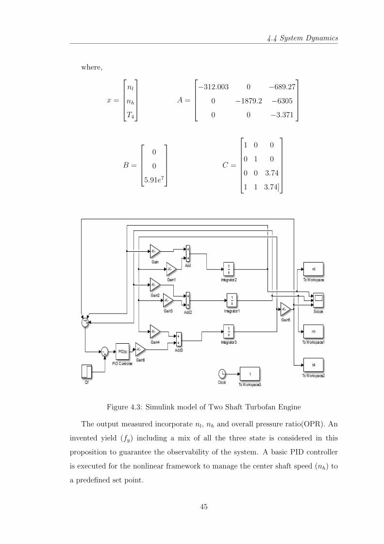
Figure 4.3: Simulink model of Two Shaft Turbofan Engine

The output measured incorporate nl, nh and overall pressure ratio(OPR). An

invented yield (fy) including a mix of all the three state is considered in this

proposition to guarantee the observability of the system. A basic PID controller

is executed for the nonlinear framework to manage the center shaft speed (nh) to

a predefined set point.

45

4.4 System Dynamics

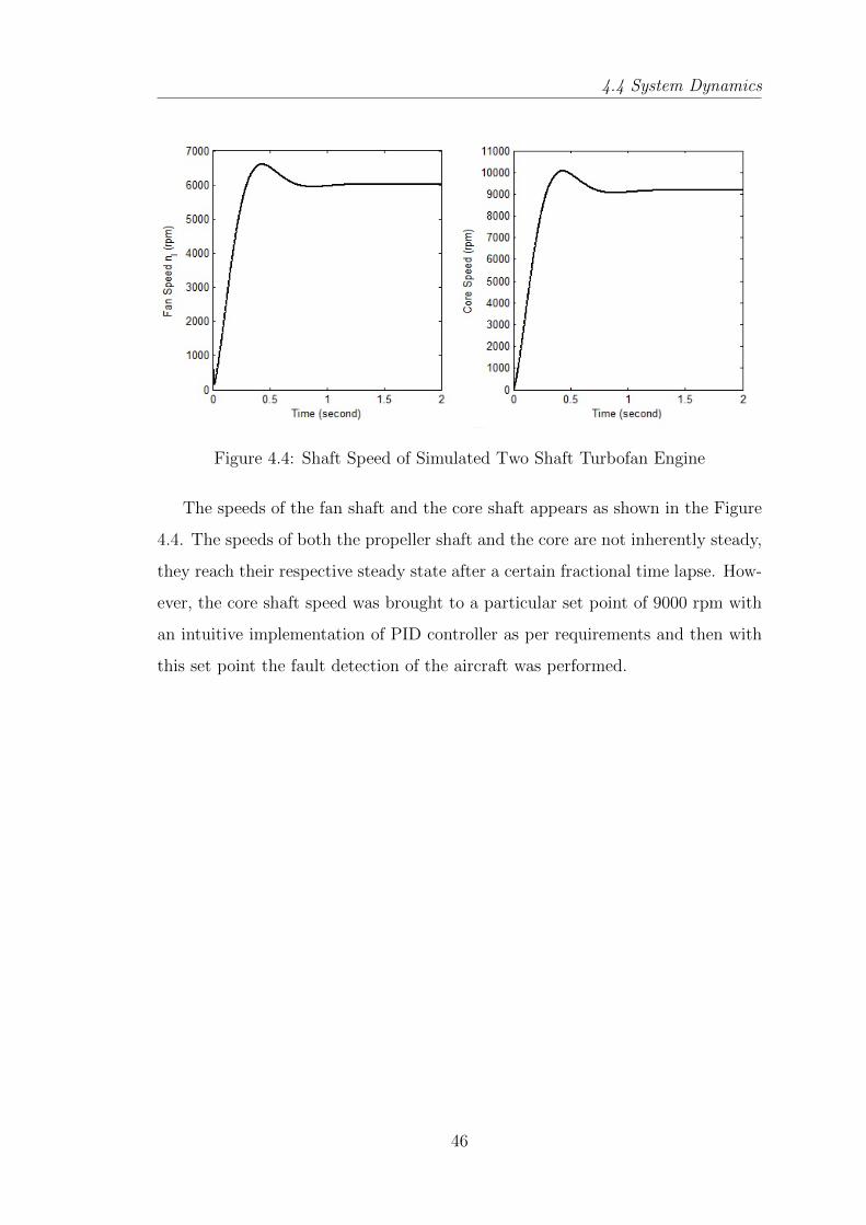
Figure 4.4: Shaft Speed of Simulated Two Shaft Turbofan Engine

The speeds of the fan shaft and the core shaft appears as shown in the Figure

4.4. The speeds of both the propeller shaft and the core are not inherently steady,

they reach their respective steady state after a certain fractional time lapse. How-

ever, the core shaft speed was brought to a particular set point of 9000 rpm with

an intuitive implementation of PID controller as per requirements and then with

this set point the fault detection of the aircraft was performed.

46

Fault Detection & IsolationStrategy

Chapter 5

Fault Detection and IsolationStrategy

A fault diagnosis scheme for aircraft engine signifies the shortcoming location

and its seclusion. Issue identification and separation plan assumes a pivotal part in

upgrading the well being, unwavering quality and diminishing the working expense

of aircraft propulsion system. Then again, accomplishing the issue identification

and separation plan with high unwavering quality is a testing issue. For this rea-

son, different methodologies have been proposed.

Some of the approaches used in fault detection and isolation scheme are Kalman

filtering, neural networks and hybrid diagnosis. Numerous current shortcoming

identification and seclusion plan are in light of the suspicion that the system shows

straight conduct in the area of the enduring state working focuses. Consequently,

linearization based symptomatic plan are frequently utilized. Since the elements

of the air ship motor are profoundly nonlinear, therefore traditional linear model

Kalman filter method, subjected to linear uncertainties is used.

5.1 Fault Detection and Isolation Logic

To outline the issue location and segregation plan for the flying machine motor

a shortcoming discovery estimator is utilized to screen the event of the flaw and

a bank of Kalman channels are utilized to focus the specific deficiency sort. The

48

5.1 Fault Detection and Isolation Logic

methodology utilized model based flaw recognition is made out of two stages. To

start with produce the lingering sign from the sensor estimation and their Kalman

channel assessed qualities and second contrast the residual with threshold to make

shortcoming identification.

The Kalman Filter is an estimator for the straight quadratic issue, which is the

issue of evaluating the immediate condition of a direct element system annoyed by

repetitive noise by utilizing estimations straightly identified with the state how-

ever defiled by background noise. To control a dynamic framework, it is crucial

to know the whole condition of the framework. For applications where it is not

generally conceivable to quantify each variable that requirements to be controlled,

the Kalman channel gives an intends to gathering the missing data from indirect

(and noisy) estimations.

Figure 5.1: Block Diagram of the Fault Detection and Isolation Strategy

With the Engine Simulation display that was produced, the model-based de-

ficiency identification methodology is executed, which comprises of a bank of

Kalman channels that is utilized for sensor flaw discovery and detachment. Each

49

5.2 Identification of Sensor Fault

Kalman channel is intended for identifying a particular sensor shortcoming. If

a sensor flaw does happen, all channels with the exception of the one utilizing

the right theory will deliver vast estimation lapses, subsequently disengaging the

sensor that has fizzled.

A linear model of the engine simulated model is represented by the following

state space equations

xs = Asxs +Bsu+ ω

ys = Csx+Dsu+ ν (5.1)

where, ω and ν are the process and sensor noise respectively, the are both

assumed to be white Gaussian noise. Their covariance matrices are

E[ω(tt)] = 0

E[ν(tt)] = 0

E[ω(tt + τt)ωT (tt)] = Qδ(τt)

E[ν(tt + τt)νT (tt)] = Rδ(τt)

The estimated state vector xs, sensor measurement ys and the kalman gain

matrix K can be calculated as

˙xs = Asxs +Bsu+K(ys − ys)

ys = Csxs

K = PCTs R−1 (5.2)

where, innovation matrix P is calculated by utilizing the linear Riccati equa-

tion.


A bank of ”n” Kalman Filter (n is the number of yields) is utilized to execute the

sensor flaw recognition logic. As said, the control info and a subset of the sensor

50


yield estimations are encouraged to each of the ”n” Kalman filter. The sensor that

is not utilized by a specific channel is the one being checked by that channel for flaw

location. Thus every channel assesses the expanded state vector utilizing (n 1)

sensors. Consequently if sensor ”i” is defective, all channels will utilize a debased

estimation, aside from channel ”i”. Channel ”i” will accordingly have the capacity

to gauge the expanded state vector from issue free sensor estimations, though the

assessments of the remaining channels will be misshaped by the flaw in sensor ”i”.

When the expanded state vector appraisal is found, the sensor estimations can be

assessed utilizing the Kalman Filter arrangement of mathematical statement. For

each filter, the residual vector is generated

rj = ysj − yjs

Consequently with the recreated motor model each of the 4 Kalman Filters

gauges the yield utilizing 3 sensor estimations (flawed) and the control data. For

this situation, since the sensor estimation 2 is flawed, all channels with the excep-

tion of channel 2 will utilize an adulterated estimation. Channel 2 will hence have

the capacity to gauge the motor yields from issue free sensor estimations, while

the yield appraisals of the remaining channels (i.e., channels 1, 3 and 4) will be

misshaped by the deficiency in sensor 2.

As we got the residual, the Weighted Sum of Squares Residual (WSSR) for

each Kalman filter can be calculated as

W j = V jrjT

Σ−1rj

It contains two hypotheses as

• System operate normally if, Threshold value for a particular sensor is greater

then the weighted sum of squares residual of that sensor.

• Fault in the system if, Threshold value for a particular sensor is less then

the weighted sum of squares residual of that sensor.

Using above two hypotheses we can identify and seclude the presence of faults

and the false alarm.

51

5.3 Fault Identification and Isolation for the Modeled Aircraft Engine

5.3 Fault Identification and Isolation for the Mod-

eled Aircraft Engine

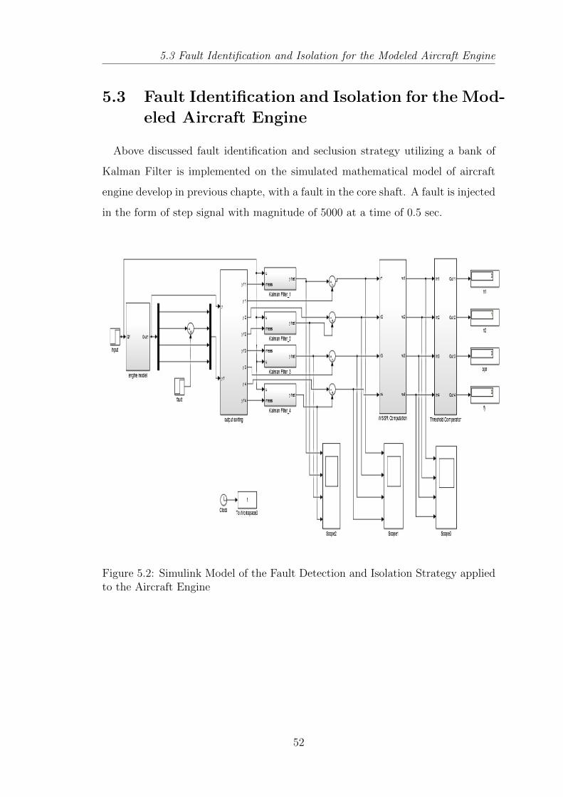
Above discussed fault identification and seclusion strategy utilizing a bank of

Kalman Filter is implemented on the simulated mathematical model of aircraft

engine develop in previous chapte, with a fault in the core shaft. A fault is injected

in the form of step signal with magnitude of 5000 at a time of 0.5 sec.

Figure 5.2: Simulink Model of the Fault Detection and Isolation Strategy appliedto the Aircraft Engine

52


5.3.1 No Sensor Fault

The estimated values of the sensor output for all the Kalman filter are shown

in figure below

Figure 5.3: Estimated Output of Kalman Filter 1


53




54


5.3.2 Fault in the Core Shaft Speed Measurement Sensor

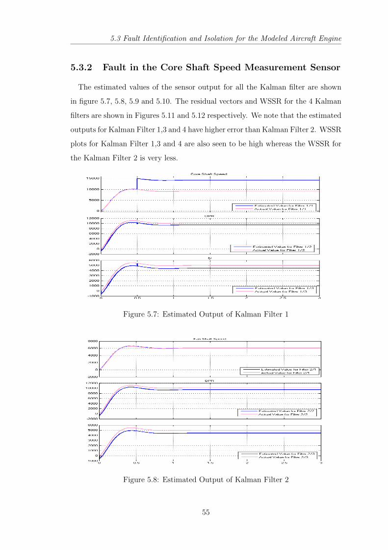
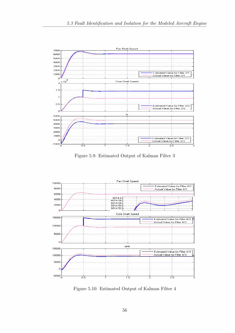
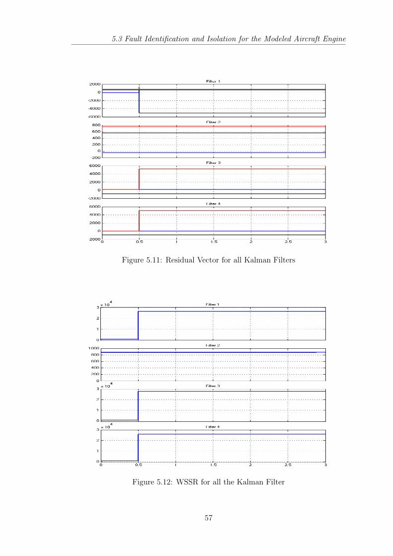
The estimated values of the sensor output for all the Kalman filter are shown

in figure 5.7, 5.8, 5.9 and 5.10. The residual vectors and WSSR for the 4 Kalman

filters are shown in Figures 5.11 and 5.12 respectively. We note that the estimated

outputs for Kalman Filter 1,3 and 4 have higher error than Kalman Filter 2. WSSR

plots for Kalman Filter 1,3 and 4 are also seen to be high whereas the WSSR for

the Kalman Filter 2 is very less.



55




56


Figure 5.11: Residual Vector for all Kalman Filters

Figure 5.12: WSSR for all the Kalman Filter

57


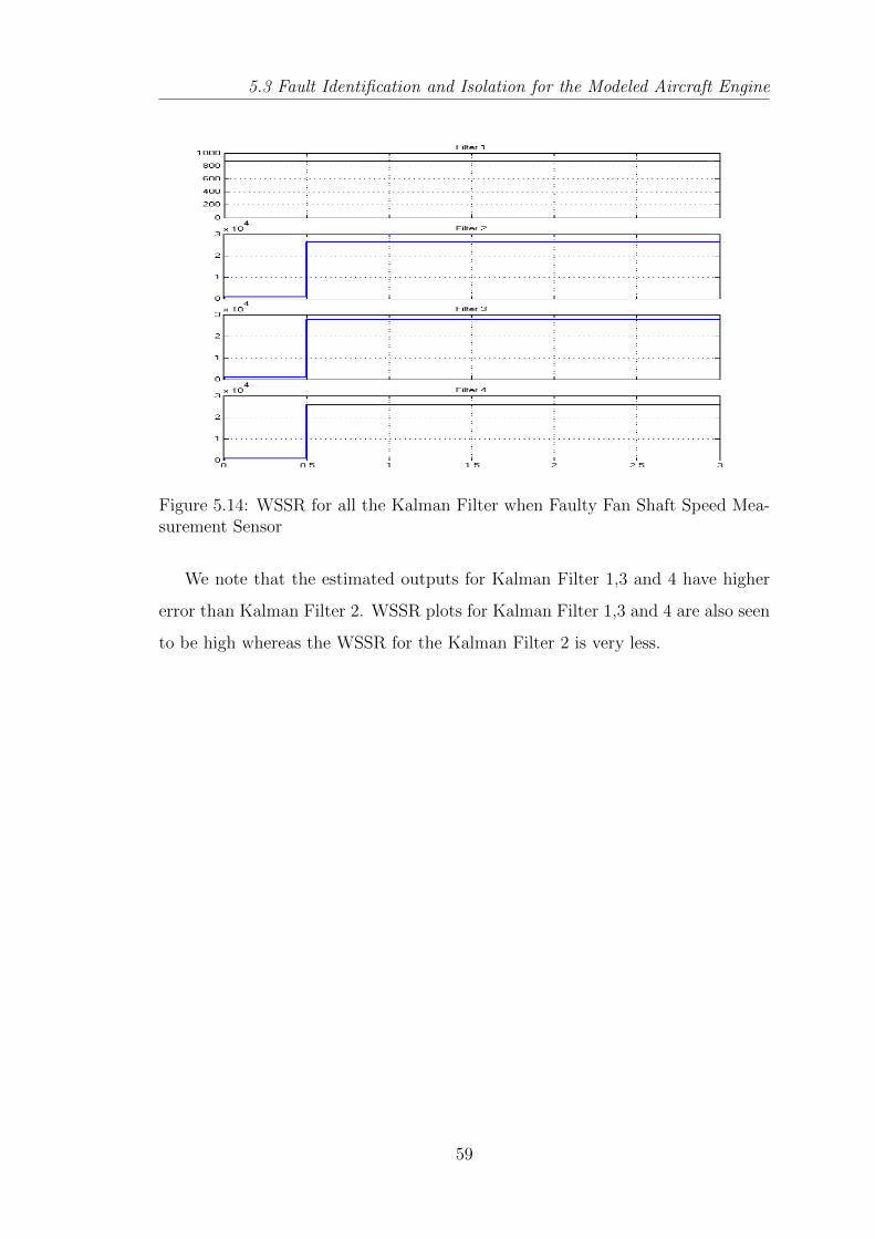
5.3.3 Fault in the Fan Shaft Speed Measurement Sensor

A fault is injected in the form of step signal with magnitude of 5000 at a time

of 0.5 sec. The residual vectors and WSSR for the 4 Kalman filters are shown in

Figures 5.13 and 5.14 respectively.

Figure 5.13: Residual Vector for all Kalman Filters when Faulty Fan Shaft SpeedMeasurement Sensor

58


Figure 5.14: WSSR for all the Kalman Filter when Faulty Fan Shaft Speed Mea-surement Sensor

We note that the estimated outputs for Kalman Filter 1,3 and 4 have higher

error than Kalman Filter 2. WSSR plots for Kalman Filter 1,3 and 4 are also seen

to be high whereas the WSSR for the Kalman Filter 2 is very less.

59

Conclusions &Scope for the Future Work

Chapter 6

Conclusion and Scope for FutureWork

6.1 Conclusion

A model of an aircraft system has been designed in an efficient way. The model

of Pitch, Roll and Sideslip control of the aircraft is very helpful in developing a

control strategy for actual system. Pitch, Roll and Sideslip control of an aircraft

is a system which require a controller to maintain the angle at its desired value.

This can be achieved by reducing the error signal, which is the difference between

output signal and desired signal. The control approach of the Model Predictive

Controller is capable of controlling the Pitch, Roll and Sideslip angle of the air-

craft system. Simulation results show that Model Predictive controller give better

performances.

Futher, this thesis focuses on an aircraft engine system, which is modeled uti-

lizing Matlab / Simulink to ensure the identification and seclusion of the faulty

sensor outputs. A fault identification and seclusion strategy, utilizing a bank of

Kalman Filters, has been developed. The simulation result obtained envisages that

the fault detection and isolation strategy developed utilizing the bank of Kalman

Filter has been able to identify and isolate the faulty sensor output in the aircraft

engine system.

61

6.2 Scope for Future Work

6.2 Scope for Future Work

For advance work, effort can be devoted in designing the more robust control

techniques for the control of the angles of roll, pitch and sideslip. Further, effort

can be made in developing the fault identification and seclusion strategy for the

actuator of the aircraft engine system utilizing the robust Kalman filter.

62

Bibliography

[1] X. Zhang, L. Tang, J. Decastro,“Robust Fault Diagnosis of Aircraft En-

gine,”IEEE Transaction on Control System Technology, Vol. 21, No.3, May

2013.

[2] T. I. Fossen,“Mathematical Model for Control of Aircraft and Satellite,”2nd

edition, NTNU, 2011. http://www.Itk.ntnu.no/fag/TTK4190/lecture_

notes/2012/Aircraft%20Fossen%202011.pdf.

[3] D. Caughey,“Introduction to Aircraft Stability and Control,”course

notes, Cornell University. https://courses.cit.cornell.edu/mae5070/

Caughey_2011_04.pdf

[4] J. Blakelock,“Automatic Control of Aircraft and Missile,”2nd edition, John

Wiley and Sons, 2011.

[5] M.V. Cook,“Flight Dynamics principles,”2nd edition, Elsevier Series, 2007.

[6] E. N. Hartley, J. L. Jerez, A. Suardi, J. M. Maciejowski, E. C. Kerrigan, and

A. Constantinides,“Predictive Control Using an FPGA with Application to

Aircraft Control,”IEEE Transactions On Control Systems Technology, Vol.

22, No. 3, May 2014.

[7] K. R. Muskea,, T.A. Badgwell,“Disturbance Modeling for Offset-free Linear

Model Predictive Control,”Journal Of Process Control, Vol. 12, No. 5, PP:

617632, 2002.

63

Bibliography

[8] Bemporad, M. Morari, V. Dua and E. N. Pistikopoulos,“The Explicit Linear

Quadratic Regulator for Constrained Systems,”Automatica, Vol. 38, No. 1,

PP: 320, Jan. 2002.

[9] J. M. Maciejowski,“Predictive Control with Constraints,”Prentice-hall, 2002.

[10] Liuping Wang,“Model Predictive Control System Design and Implementation

Using MATLAB.”Springer, 2009.

[11] Labane Chrif, Z. M. Kadda,“Aircraft Control System Using LQG and LQR

Controller with Optimal Estimation-Kalman Filter Design,”Elsevier, Proce-

dia Engineering, 80, (2014): 245 257.

[12] R. Lungu, A. N. Tudosie and L. Dinca,“Double-Spool Single Jet Engine for

Aircraft as Controlled Object,”International Journal Of Mathematical Models

And Methods In Applied Sciences, Issue 4, Volume 2, 2008.

[13] Y.S. Guan, J.S. Warng and T. Lee,“A new method of digital simulation for an

aircraft gas turbine engine control system,”Applied Mathematical Modeling,

Vol. 11, Issue 6, (1987):458 -464.

[14] H.A. Spang III and H. Brown,“Control of Jet Engine,”Elsevier, Control En-

gineering Practice, Vol. 7, Issue 9,(1999): 10431059.

[15] Al Behbahani, R.K. Yedavalli, P. Shankar, and M. Siddiqi,“Modeling, Diag-

nostics and Prognostics of a Two Spool Turbine Engine,”41st Joint Propulsion

Conference, AIAA, 2005.

[16] C. Kong and J. Park,“Transient Performance Simulation of Propulsion Sys-

tem for CRW Type UAV Using SIMULINK,”24th International Congress of

the Aeronautical Science, 2004.

[17] O. Turan, H. Aydn, T.H. Karakoc and A. Midilli,“First Law Approach of a

Low Bypass Turbofan Engine,”Journal of Automation and Control Engineer-

ing, Vol. 2, Issue 1, 2014.

64

Bibliography

[18] M. Grewal and A. Andrews,“Kalman Filtering : Theory and Practice Using

MATLAB,”2nd edition, John Wiley and Sons, 2001.

[19] W. Xue, Y.Q. Guo and X.D. Zhang,“A Bank of Kalman Filters And Ro-

bust Kalman Filter Applied in Fault Diagnosis of Aircraft Engine Sen-

sor/Actuator,”Proceedings Of The Second International Conference On In-

novative Computing, Informatio And Control, 2007.

[20] W. Chen and M. Saif,“Adaptive actuator fault detection, isolation and ac-

commodation in uncertain systems,”International Journal of Control, 80:1,

(2007):45-63.

[21] A. Alexiou and K. Mathioudakis,“Gas Turbine Engine Performance Model

Applications Using an Object-Oriented Simulation Tool,”ASME Turbo Expo

2006: Power for Land, Sea, and Air. American Society of Mechanical Engi-

neers 2006.

[22] F. Correa, A. Oliviera and R. Bosa,“Dynamic Modelling Nonlinear and Con-

trol System for a Turboshaft,”Proceedings of 12th Pan American Congress of

Applied Mechanics, 2012.

[23] C. Kong, M. Kang and G. Park,“Study on Condition Monitoring of Two Spool

Turbofan Engine using Non-Linear Gas Path Analysis Method and Genetic

Algorithms,”International Journal of Materials, Mechanics and Manufactur-

ing, 1.2 (2013): 214-220.

[24] M. Kale and A. J. Chipperfield,“Stabilized MPC Formulations for Robust Re-

configurable Flight Control,”Control Engineering Practice, 13.6 (2005): 771-

788.

[25] W. Merrill, J. DeLaat and W. Bruton“Advanced Detection, Isolation and Ac-

commodation of Sensor Failures Real Time Evaluation,”Journal of Guidance,

Control, and Dynamics, 11.6 (1988): 517-526.

65

Bibliography

[26] M.Seok and B. Jung,“Speed and Surge Control for an Unmanned Aircraft

Vehicle with Turbojet Engine,”Computer Science and Convergence, Springer,

(2012): 735-743.

[27] Feng Lu, Y. Lv, J. Huang and X. Qiu,“A Model Based Approach for Gas

Turbine Engine Performance Optimal Estimation,”Asian Journal of Control,

15.6 (2013): 1794-1808.

[28] F. Caliskan and C. Hacizade,“Sensor and Actuator FDI Applied to an UAV

Dynamic Model,”Preprints of the 19th World Congress, The International

Federation of Automatic Control, 2014.

66

Documents

Modeling and Control of an Aircraft Systemethesis.nitrkl.ac.in/7821/1/2015_MT_Modeling_Gupta.pdf · Modeling and Control of an Aircraft System (for Aerospace Applications) Dissertation