Embed Size (px)
Citation preview

i
Modeling and Experimental Validation of a Low-Lift, Vapor
Compression Heat Pump By Muhammad Tauha Ali
A Thesis Presented to the Masdar Institute of Science and Technology in Partial
Fulfillment of the Requirements for the Degree of
Master of Science in Mechanical Engineering
August 2011
© 2011 Masdar Institute of Science and Technology
All rights reserved
AUTHOR’S DECLARATION
I understand that copyright in my thesis is transferred
to Masdar Institute of Science and Technology.
Author ____________________________________
RESEARCH SUPERVISORY COMMITTEE MEMBERS
Dr. Peter Armstrong, Chair, _______________________________________________
Masdar Institute of Science and Technology
Dr. Matteo Chiesa, _____________________________________________________
Masdar Institute of Science and Technology
Dr. Scott Kennedy, ______________________________________________________
Masdar Institute of Science and Technology

ii
Abstract In this study, a heat pump test stand and a test chamber have been built for assessment of
the energy savings of low-lift radiant-cooling cooling technology with pre-cooling control. The
heat pump test stand has been built from a conventional split unit heat pump to be able to operate
in either Direct Expansion (DX) mode or Chiller mode. A central data acquisition and control
system has been developed for controlling compressor speed, condenser fan speed and expansion
valve position. Component models have been developed from first principles to model the
performance of the heat pump in DX mode or Chiller mode. The objective of this study is to
present a system model based on first principles with minimum parameters estimation. The
system model is found to accurately predict the system COP within ±20% for both Chiller mode
and DX mode operation for majority of data points. Assessment of the effect of refrigerant oil on
heat pump performance is also provided. The refrigerant oil tends to increase heat transfer in the
fan-coil condenser and brazed-plate evaporator. However, at low refrigerant flow rates, the heat
transfer was found to decrease for fan-coil condenser. The pressure drop was found to increase in
the heat exchangers with inclusion of oil. A comparison between the component models
developed in this study and those presented in (Zakula, 2010) is also given. The models
developed in this study provide better estimation of system parameters especially for pressure
drop. Equations for controlling condenser and compressor fan speeds during pre-cooling control
for optimal operation based on the optimization results presented in (Zakula, 2010) are also
presented for use in pre-cooling control.
iii
This research was supported by the Government of Abu Dhabi to help fulfill the
vision of the late President Sheikh Zayed Bin Sultan Al Nayhan for sustainable
development and empowerment of the UAE and humankind.

iv
Acknowledgments
I am firstly grateful to Almighty Allah for giving me the strength and ability to carry out this
study. Secondly, I like to thanks Dr. Peter Armstrong for his thoughtful and wide-ranging advice
throughout the study. I am grateful to all my friends especially Arslan Khalid for his stepper
motor circuit used for controlling of the expansion valve, Zaid Thaboub and Abdul Qadir for
assisting me in insulation of test chamber and Marwan Mokhtar for providing me initial guidance
on instrumentation. I like to acknowledge my colleagues at Massachusetts Institute of
Technology, Nicholas Gayeski for laying down the foundation of my experimental work and
providing me his test stands experimental data set, Tea Zakula for sending me the MATLAB
code of her heat exchanger models and Ryan Willingham for providing me the start in learning
of CRBasic and Acetylene welding. I also want to thank Masdar security guards who provided
the necessary assistance in times of need while preparing the test facility. Lastly, I like to thank
my family for nourishing me during my course of work.
v
1 Contents
1 Introduction ............................................................................................................................. 1
2 Literature Review .................................................................................................................... 3
2.1 Variable Speed Compressors ........................................................................................... 3
2.2 Vapor Compression Equipment Modeling ....................................................................... 5
2.3 Heat Exchanger Modeling ................................................................................................ 7
2.4 Oil Effect on Vapor Compression System ..................................................................... 12
3 Component Modeling ............................................................................................................ 14
3.1 Vapor Compression Cycle ............................................................................................. 14
3.2 Refrigerant Oil-Mixture Modeling ................................................................................. 15
3.3 Compressor..................................................................................................................... 20
3.3.1 Compressor Model Description .............................................................................. 26
3.4 Fan-Coil Heat Exchanger Model .................................................................................... 28
3.4.1 Fin Efficiency and Air-Side Heat Transfer Coefficient .......................................... 30
3.4.2 Single-Phase Refrigerant Side Heat Transfer ......................................................... 32
3.4.3 Single-Phase Refrigerant-Side Pressure Drop ........................................................ 33
3.4.4 Flow Pattern Map .................................................................................................... 33
3.4.5 Two-Phase Refrigerant-Side Heat Transfer ............................................................ 38
vi
3.4.6 Two-Phase Refrigerant-Side Pressure Drop ........................................................... 42
3.4.7 Condenser Model Description ................................................................................ 47
3.4.8 Fan-Coil Evaporator Model Description ................................................................ 53
3.5 Plate Heat Exchanger Model .......................................................................................... 58
3.5.1 Single-Phase Refrigerant Side Heat Transfer ......................................................... 58
3.5.2 Single-Phase Refrigerant-Side Pressure Drop ........................................................ 59
3.5.3 Two-Phase Refrigerant-Side Heat Transfer ............................................................ 60
3.5.4 Two-Phase Refrigerant-Side Pressure Drop ........................................................... 61
3.5.5 Port Pressure Drop .................................................................................................. 62
3.5.6 Plate Evaporator Model Description ....................................................................... 63
3.6 System Model ................................................................................................................. 68
4 Experimental Setup and Instrumentation .............................................................................. 72
4.1 Test Stand Description ................................................................................................... 72
4.2 Test Chamber Description .............................................................................................. 74
4.3 Experimental Data Set .................................................................................................... 77
4.4 Calibration of Pressure Transducers .............................................................................. 78
4.5 Condenser Fan Characterization .................................................................................... 79
4.6 LEV Control Verification ............................................................................................... 80
4.7 DX Mode Operation for Component Models Verification ............................................ 83
4.8 Chiller Mode Operation for Component Models Verification ....................................... 85
vii
4.9 Energy Balance Check for the Experimental Data Set .................................................. 86
4.9.1 DX Mode Operation ............................................................................................... 87
4.9.2 Chiller Mode Operation .......................................................................................... 89
5 Experimental Validation of Models ...................................................................................... 91
5.1 Compressor Model ......................................................................................................... 91
5.2 Condenser Model ........................................................................................................... 95
5.3 Fan-Coil Evaporator Model ........................................................................................... 99
5.4 Plate Evaporator Model ................................................................................................ 102
5.5 Oil Concentration Effect on Vapor Compression Components: .................................. 105
5.5.1 Compressor: .......................................................................................................... 105
5.5.2 Condenser: ............................................................................................................ 106
5.5.3 Evaporator: ............................................................................................................ 107
5.6 System Model ............................................................................................................... 108
5.7 Optimal Performance Map for Control of Compressor Speed and Outdoor Fan Speed
111
5.7.1 DX Mode .............................................................................................................. 112
5.7.2 Chiller Mode ......................................................................................................... 112
6 Conclusion and Future Work ............................................................................................... 116
6.1 Conclusion .................................................................................................................... 116
6.2 Future Work ................................................................................................................. 118

viii
7 Test Stand Components and Instrumentation Description .................................................. 120
8 Data Logging and Controlling Code for Test Stand Instruments ........................................ 125
9 Test Chamber Heat Transfer Reduction after Insulation ..................................................... 135
10 Air Leakage Testing of Test Chamber ............................................................................. 136
10.1 Air Leakage before Caulking: ...................................................................................... 136
10.2 Air Leakage after Caulking: ......................................................................................... 137
11 Test Chamber Components and Thermocouple Location Description ............................ 138
12 Gauge Pressure Sensor/ Transducer Calibration Procedure ............................................ 139
13 Test Stand Data for DX Mode of Operation .................................................................... 142
14 Test Stand Data for Chiller Mode of Operation............................................................... 148
15 Nomenclature ................................................................................................................... 152
16 Bibliography .................................................................................................................... 155

ix
List of Tables
Table 3.1: Comparison of mass flow rate models ......................................................................... 22
Table 3.2: Coefficients and accuracy of mass and power models ................................................ 24
Table 3.3: Compressor model parameters .................................................................................... 26
Table 3.4: Condenser model parameters ....................................................................................... 47
Table 3.5: Condenser details required .......................................................................................... 47
Table 3.6: Fan-coil evaporator model parameters ........................................................................ 53
Table 3.7: Fan-coil evaporator details required ............................................................................ 53
Table 3.8: Brazed-plate evaporator model parameters ................................................................. 63
Table 3.9: Brazed-plate evaporator details required ..................................................................... 63
Table 3.10: System model parameters .......................................................................................... 68
Table 3.11: System details required .............................................................................................. 68
Table 3.12: Fan and Pump Power Coefficients and RMSE .......................................................... 70
Table 4.1: Refrigerant charge for DX and Chiller modes of operation ........................................ 73
Table 4.2: Test Chamber Thermal Loads Description .................................................................. 77
Table 4.3: Conversion coefficients for the pressure transducers .................................................. 78
Table 4.4: PID control parameters ................................................................................................ 82
Table 5.1: Comparison of output parameters of current compressor model and model of (Zakula,
2010) ............................................................................................................................................. 94
Table 5.2: Comparison of output parameters of current condenser model and model of (Zakula,
2010) ............................................................................................................................................. 98
x
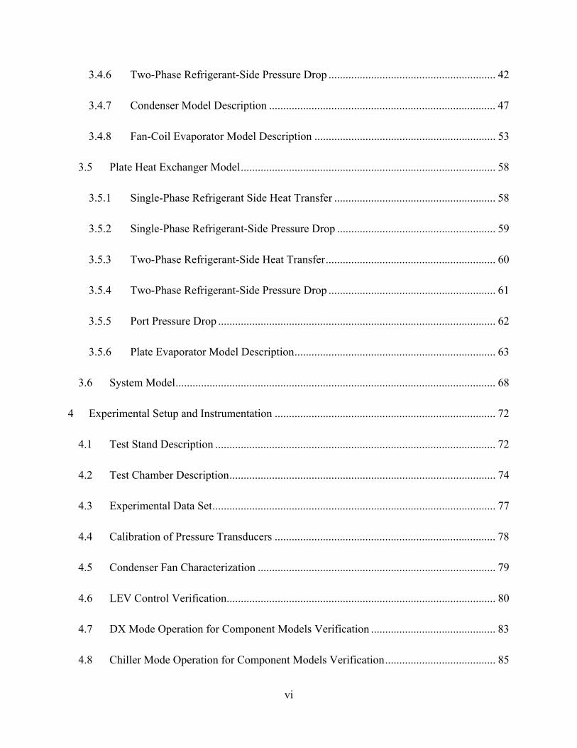
Table 5.3: Comparison of output parameters of current fan-coil evaporator model and model of
(Zakula, 2010) ............................................................................................................................. 101
Table 5.4: Comparison of output parameters of current brazed-plate evaporator model and model
of (Zakula, 2011) ........................................................................................................................ 104
Table 5.5: Output parameters of system model .......................................................................... 110
Table 5.6: Coefficients for optimal compressor and condenser speed control equations ........... 113
Table 7.1: Test stand and test chamber components description ................................................ 120
Table 7.2: Test stand and test chamber sensors description ....................................................... 123

xi
List of Figures
Figure 3.1: T-s diagram of vapor compression cycle with low-lift operation illustration (P. R.
Armstrong, Jiang, Winiarski, Katipamula, & Norford, 2009) ...................................................... 14
Figure 3.2: Local oil concentration vs. vapor quality ................................................................... 17
Figure 3.3: Difference between T and T of pure refrigerant for different T vs. ω ... 19
Figure 3.4: (a) Refrigerant mass flow residual vs. compressor speed (b) Compressor power
residual vs. compressor speed (c) Refrigerant mass flow residual vs. pressure ratio (d)
Compressor power residual vs. pressure ratio .............................................................................. 24
Figure 3.5: Illustration of η vs. pressure ratio ....................................................................... 25
Figure 3.6: Compressor model flow chart .................................................................................... 27
Figure 3.7: Two-phase flow pattern map (Wojtan, Ursenbacher, & Thome, 2005a) ................... 34
Figure 3.8: (a) Condensation heat transfer model (b) Evaporation heat transfer model ............... 42
Figure 3.9: Pressure drop model ................................................................................................... 46
Figure 3.10: Condenser model flow chart ..................................................................................... 52
Figure 3.11: Fan-coil evaporator model flow chart ...................................................................... 57
Figure 3.12: Brazed-plate evaporator model flow chart ............................................................... 67
Figure 3.13: System model flow chart .......................................................................................... 71
Figure 4.1: Test stand component schematic ................................................................................ 73
Figure 4.2: Test chamber with instrumentation ............................................................................ 75
Figure 4.3: (a) Pressure residuals before calibration (b) Pressure residuals after calibration ....... 79
Figure 4.4: Condenser fan characterization .................................................................................. 80
Figure 4.5: LEV control circuit schematic (Arslan Khalid, 2011) ............................................... 81
xii
Figure 4.6: LEV control accuracy with suction superheat as control variable ............................. 83
Figure 4.7: System COP plotted against (a) Compressor speed and (b) Pressure ratio ................ 84
Figure 4.8: System COP plotted against (a) Compressor speed and (b) Pressure ratio ................ 85
Figure 4.9: (a) Compressor energy balance check (b) Condenser energy balance check (c) Fan-
coil evaporator energy balance (d) System energy balance check. Lines at ±20% are shown in
(a)-(c) and at ±5% in (d) ............................................................................................................... 87
Figure 4.10: (a) Compressor energy balance check (b) Condenser energy balance check (c)
Brazed-plate evaporator energy balance (d) System energy balance check. Lines at ±20% are
shown in (a)-(c) and at ±5% in (d) ................................................................................................ 89
Figure 5.1: (a) Compressor speed residual vs. compressor speed (b) Compressor speed residual
vs. compressor speed (c) Compressor power residuals vs. compressor power (d) Compressor
power residuals vs. compressor power ......................................................................................... 92
Figure 5.2: (a) T residuals vs. compressor speed (b) COP compressor residuals vs. pressure
ratio ............................................................................................................................................... 92
Figure 5.3: (a) ε residuals vs. measured ε (b) P residuals vs. refrigerant flow rate
(c) T residuals vs. refrigerant flow rate ............................................................................. 96
Figure 5.4: (a) Heat rejected and (b) dP difference between no oil and 1% oil ..................... 97
Figure 5.5: (a) ε residuals vs. measured ε (b) P residuals vs. compressor speed (c)
T residuals vs. compressor speed ........................................................................................ 99
Figure 5.6: (a) Heat rejected and (b) dP difference between no oil and 1% oil ................... 100
Figure 5.7: (a) ε residuals vs. measured ε (b) P residuals vs. refrigerant flow rate
(c) T residuals vs. refrigerant flow rate (d) T residuals vs. refrigerant flow rate . 102
Figure 5.8: (a) Heat rejected and (b) dP difference between no oil and 1% oil ................... 103

xiii
Figure 5.9: Oil concentration effect on (a) Compressor speed (b) Compressor power (c)
Discharge temperature (d) Compressor COP ............................................................................. 105
Figure 5.10: Oil concentration effect on condenser (a) Outlet pressure (b) Outlet temperature and
(c) Effectiveness .......................................................................................................................... 106
Figure 5.11: Oil concentration effect on evaporator (a) Outlet pressure (b) Outlet temperature (c)
Outlet water temperature and (d) Effectiveness .......................................................................... 107
Figure 5.12: (a) Compressor speed residual vs. compressor speed (b) V residual vs. V
(c) V residual vs. V (d) System COP residuals vs. measured system COP .............. 108
Figure 5.13: (a) Compressor speed residuals vs. measured compressor speed (b) V
residuals vs. measured V (c) V residuals vs. measured V (d) System COP
residuals vs. measured system COP............................................................................................ 109
Figure 5.14: Illustration of optimal compressor speeds for DX and chiller mode operation for a
given Q , T and T ................................................................................................................. 114
Figure 5.15: Illustration of optimal condenser fan speeds for DX and chiller mode operation for a
given Q , T and T ................................................................................................................. 115

Chapter 1: Introduction
1
CHAPTER 1
1 Introduction
Global warming is both a cause and effect of the use of active air-conditioning systems for
maintaining comfort level for humans. Buildings account for over 40% of primary energy usage
in the world (World Building Council for Sustainable Development (WBCSD), 2008). Around
30% (Radhi, 2009; US Department of Energy, 2010) of this energy is used for air conditioning.
For hot and humid climates, such as in United Arab Emirates (UAE), this share can reach 40%
and on the peak day exceeds 60% of buildings energy use (Ali, Mokhtar, Chiesa, & P.
Armstrong, 2011; Radhi, 2009). Due to global warming and increase in energy costs, efforts are
being made to enhance the efficiency of air-conditioning equipment by imposing efficiency
standards; use of low-energy cooling technologies and by improving the building envelope to
reduce cooling/heating loads.
One of the most common methods of increasing equipment efficiency is through implementing
variable speed drives in electric motors to match demand. The savings achieved over constant
electric drives are reported between 20%-40% (Qureshi & Tassou, 1996; Shimma, Tateuchi, &
Sugiura, 1985). Another method for achieving over 40% increase in system efficiency is through
radiant cooling (Feustel & Stetiu, 1995; Roth, Westphalen, Dieckmann, S. D. Hamilton, &
Goetzler, 2002). The radiant cooling system only handles sensible loads. Therefore, a separate
ventilation system is needed to replace humid air with dry air (Feustel & Stetiu, 1995; Niu, L. Z.
Zhang, & Zuo, 2002). Among the different types of ventilation systems available for handling

Chapter 1: Introduction
2
latent loads, desiccant dehumidification can achieve up to 25% energy savings over conventional
systems (Michael D. Larrañaga, Mario G. Beruvides, H.W. Holder, Enusha Karunasena, &
David C. Straus, 2008). For Abu Dhabi, it is estimated that sensible cooling accounts for around
80% of the buildings cooling load (Ali et al., 2011). Implementation of low-lift, radiant cooling
with pre-cooling control can reduce this load by around 70% for Abu Dhabi (P. R. Armstrong,
Jiang, Winiarski, Katipamula, & Norford, 2009).
This study is part of the low-lift, radiant-cooling with pre-cooling control project being carried
out at Masdar Institute (MI), Massachusetts Institute of Technology (MIT) and Pacific Northwest
National Laboratory (PNNL). In this study, modeling and experimental validation of
conventional vapor compression Direct Expansion (DX) unit equipped with variable speed
compressor, condenser and evaporator fan is presented. In chiller mode of operation, the
evaporator is modeled as a brazed-plate heat exchanger (HX). The objective of this study is to
present a system model based on first principles with minimum parameters estimation.
Chapter 2 presents a review of variable speed compressor savings reported in the literature,
system and component models of vapor compression equipment and refrigerant-oil effect on the
performance of vapor compression equipment. Component models of the system and the system
model are presented in Chapter 3. In Chapter 4, details of experimental setup and instrumentation
accuracy are described. Experimental verification of component models and the system model,
assessment of effect of refrigerant oil on component models and comparison of the results
between the models developed in this study with the models presented in (Zakula, 2010) is
presented in Chapter 5. Equations for controlling compressor and condenser speed based on the
optimization results of (Zakula, 2010) are also given to be used in pre-cooling control. Lastly,
conclusion and directions for future work are presented in Chapter 6.
Chapter 2: Literature Review
3
CHAPTER 2
2 Literature Review
2.1 Variable Speed Compressors
In conventional vapor compression equipment, the compressor is driven by a constant speed
electric motor. Cooling capacity control is achieved by cylinder unloading, throttling at suction ,
clearance volume change or by on-off cycling in reciprocating compressors, slide valve position
change in rotary or scroll compressors and screw compressors, and changing position of inlet
guide vanes in centrifugal compressors (Brown, 1997). Through advancement in electronics
technology, speed modulation of electric motors can now be achieved by varying the frequency
of power supply. The first reported savings potential of variable capacity control by the use of
variable frequency drives (VFD) was presented in (Cohen, J. F. Hamilton, & Pearson, 1974). A
system with constant compressor speed, condenser and evaporator fan speed was compared to a
system with variable speed compressor, condenser and evaporator fan. Seasonal savings of 28-
35% were reported for climates at mid-latitude in US. The savings were mainly attributed to
reduced cycling losses, lower condensing temperatures and higher evaporating temperatures at
part-loads. In (Qureshi & Tassou, 1996), a comprehensive review of the efforts made to measure
the savings potential at residential and commercial level is given. The effects on electrical and
mechanical aspects of equipment operation during variable speed are also reviewed.
Chapter 2: Literature Review
4
The mechanical advantages of variable speed compressors most often cited are reduced cycling
losses by varying the capacity to meet the demand, accurate temperature control, compressor
soft-start and low noise operation (Lida, Yamamoto, Kuroda, & Hibi, 1982). The reduction in
pressure ratio from closer approach temperatures also results in increased compressor
performance and cycle performance (P. R. Armstrong, Jiang, Winiarski, Katipamula, Norford, et
al., 2009; Qureshi & Tassou, 1996; Shimma et al., 1985). The side-effects of implementing
inverter drive control are mainly due to harmonics in waveform resulting from waveform
modulation. They increase motor losses due to non-sinusoidal waveform, variation in slip of
induction motor and torque oscillations resulting in extra stress on windings (Qureshi & Tassou,
1996). It was mentioned by (Rice, 1988) that use of permanent-magnet motor will reduce the slip
losses.
Air-conditioning equipment runs on part-load most of the time (Cohen et al., 1974). As
mentioned earlier, modulation of the capacity of vapor compression equipment at part-load
increases system efficiency due to decreased thermal load for the same heat transfer area. Recent
studies (Gayeski, 2010; Gayeski, Zakula, P. R. Armstrong, & Norford, 2010), investigated this
effect on a variable speed compressor by running it at low speeds which resulted in very high
Coefficient of Performance (COP). This operation of the compressor is termed as low-lift
operation as minimum rise in pressure ratio occurs to deliver the required cooling capacity.

Chapter 2: Literature Review
5
2.2 Vapor Compression Equipment Modeling
Various models of vapor compression equipment have been presented in the literature. These
models can be broadly classified into dynamic and steady state models. Transient modeling is
further classified based on the scale of transients such as system startup or compressor valve
dynamics and the methodology used in modeling of heat exchangers such as discretized or zonal.
Transient modeling of vapor compression equipment is beyond the scope of this thesis. Steady
state models of vapor compression equipment range from models based on regression of system
variables to models based on first principle analysis of components. An extensive review of these
models is provided in (Bendapudi & Braun, 2002; Jin & Spitler, 2002; Iu, 2007).
Hiller and Glicksman are considered to be among the pioneers of modeling of vapor compression
cycle’s components from first principles (Hiller & Glicksman, 1976). Their model included
modeling of compressor, expansion valve and fan-coil HX working as a condenser or evaporator.
Their model used real gas properties, accounted for oil circulation effect on compressor capacity
and employed modeling of compressor capacity control achieved through clearance volume
control or late suction valve closing. Their HX models used zone-by-zone approach which will
be explained in section 2.3. The HX models used ε-NTU method for simulation of heat transfer,
accounted for pressure drop and in the case of evaporator, effect of moisture presence on
evaporator. An empirical model for quick assessment of system performance was presented by
Allen and Hamilton (Allen & J. F. Hamilton, 1983). Their model estimated the cooling capacity
and compressor power as polynomial functions of condenser and evaporator water temperatures
and flow rates. The model of Hamilton and Miller (J. F. Hamilton & Miller, 1990) improved the
previous model of (Allen & J. F. Hamilton, 1983) by dividing the system into its components.
The component models required refrigerant condition details at the inlet and outlet of the
Chapter 2: Literature Review
6
components. The model of Fisher and Rice (Fischer, Rice, & Jackson, 1988) incorporated
detailed physical phenomena in the component models. For example, the compressor model
included the option of assessing the effect of changes in heat loss and efficiency on compressor
power. Also, variable HX conductances were modeled based on different heat transfer
phenomenon occurring in the heat exchangers. Empirical models for expansion devices were
also included in the system model. The model of Domanski and Didion (Domanski & Didion,
1984) increased the level of detail used to model system components. Damasceno (Damasceno,
Goldschmidt, & Rooke, 1990) verified the accuracy of Domanski’s model over Fisher’s. In
Domanski’s model, compressor characteristics are captured in greater detail by dividing
compressor into five components. The model account for heat transfer and pressure drop
between suction and discharge and treats the compression process as a polytropic process. The
heat exchangers are also divided into small segments using a tube-by-tube approach which will
be explained in section 2.3.
The model presented by Stefanuk (Stefanuk, Aplevich, & Renksizbulut, 1993) chooses the
approach of modeling different components based on the physical phenomenon occurring in the
components and using experimental data to determine the parameters of each component model.
The model presented by Hui Jin (Jin & Spitler, 2002) attempts to minimize the number of
parameters needed for such a model. However, certain compromises are made such as
compression and expansion processes in the compressor are considered isentropic, constant HX
conductance values are assumed and same pressure drop is considered on the discharge and
suction side of the compressor. The model presented by Armstrong (P. R. Armstrong, Jiang,
Winiarski, Katipamula, Norford, et al., 2009) follows the same approach but considers polytropic
processes in the compressor in which the polytropic exponent is modeled as a function of

Chapter 2: Literature Review
7
pressure ratio and speed. Also, the model is intended for modeling of a variable speed
compressor which is the focus of this study.
2.3 Heat Exchanger Modeling
Heat exchangers are usually modeled based on zone-by-zone, tube-by-tube or segment-by-
segment approach as described in (Browne & Bansal, 2001; Iu, 2007). In zone-by-zone
approach, the HX is divided into zones based on the type of fluid phase. For example, the
condenser is divided into de-superheating, condensing and sub-cooling portions. In segment-by-
segment or tube-by-tube approach, the HX is discretized into a finite number of elements. Heat
transfer and pressure drop calculations are then carried out progressively through the HX.
Extensive experimentation has been carried by researchers to model the air-side heat transfer for
different types of fin-tube and fin-plate heat exchangers. A comprehensive review is provided in
(Jacobi, Park, Tafti, & X. Zhang, 2001). In the review, correlations and comments on the
experimentation with fin-tube HX by the researchers are presented. Effects of fin geometry such
as fin pitch, fin type such as plain, wavy, corrugated, louvered etc, tube geometry such as round
tube and flat tube and HX operating condition such as dry, wet or frosting are covered. For plain-
fin round-tube geometry, it is reported that the heat transfer increases slightly with smaller fin
thickness while pressure drop increases for higher fin pitch with negligible influence on heat
transfer. A comparison between fin-round tube HX and fin-flat tube HX is also provided. It is
concluded that flat-tube HX have higher heat transfer compared to round-tube but during wet
operating conditions, the degradation in heat transfer for flat-tube is higher than for round tubes.

Chapter 2: Literature Review
8
The correlation of Grey and Webb (Gray & Webb, 1986) is recommended for modeling heat
transfer phenomena in plain-fin round-tube HX over a broad range of parameters.
The fin efficiency for plain-fin round-tube HX is usually calculated based on approximations
developed for the circular fin efficiency formulation (Perrotin & Clodic, 2003). The equivalent
circular fin method and the sector method can be used for calculation of fin efficiency. The fin
profile is considered to be a square for inline tubes and hexagonal for staggered tubes. In the
sector method, the fin is divided into several circular sectors based in the tube center and the fin
geometry. The sector efficiency is then evaluated from the exact solution for circular fins with an
adiabatic tip or from approximations to that solution. In the equivalent circular fin method, the
fin efficiency can be calculated by considering a circular fin having the same surface area as a
rectangular or hexagonal fin based on tube arrangements or through the Schmidt method
(Schmidt, 1949). The Schmidt method is simpler to use than the sector method in which
correlations have been developed by Schmidt to find an equivalent circular fin having the same
fin efficiency as the rectangular fin or the hexagonal fin. A comparison between the sector and
equivalent circular fin method is given in (Perrotin & Clodic, 2003). Use of equivalent circular
fin method is recommended for the case of plain fins.
Heat transfer and pressure drop in the two-phase of refrigerants have been investigated
extensively for different commercial refrigerants in the case of fin-tube HX. The two-phase heat
transfer is generally modeled through three approaches. In the enhancement model approach, the
single-phase heat transfer coefficient is multiplied by an enhancement factor. The weighted
model considers two-phase heat transfer coefficient to be a sum of convective and film/nucleate
condensation/boiling with appropriate weights. A variation on the weighted model is the

Chapter 2: Literature Review
9
asymptotic model in which the sum of aforementioned components is considered with
appropriate exponents (Wojtan, 2005).
The condensation or evaporation heat transfer is usually modeled by an enhancement model in
which the single-phase heat transfer coefficient is multiplied by ratio of vapor quality, viscosity
and density ratios, Martinelli parameter (Xtt)1, etc. An example of such a model is of Shah (Shah,
1979) which is extensively used because of its simplicity. A comparison of different
condensation and evaporation heat transfer correlation developed for modeling refrigerant heat
transfer in condensation is presented in (Boissieux, Heikal, & Johns, 2000a, 2000b; Cavallini et
al., 2002). It is shown that for older refrigerants such as R22, R-407C etc, the simple
enhancement models were able to predict the heat transfer coefficient within ±20%. However, it
is mentioned in (Thome, El Hajal, & Cavallini, 2003) that the enhancement model type
correlations that were developed earlier over predicts the heat transfer by 20-40% for
condensation when applied to new refrigerants working at high pressures such as R410a. A new
weighted type model is presented for which prediction of the heat transfer data is reported to be
within ±20% for a range of mass flux, tube diameters and refrigerant pressures.
The flow pattern map of Wojtan et. al (Wojtan, Ursenbacher, & Thome, 2005a) is used to
identify the different flow regimes. This map is the modified version of Thome El Hajjal map (El
Hajal, Thome, & Cavallini, 2003) which was used to develop the superposition model and
condensation heat transfer correlations for convective and film condensation. In the new map,
two flow regimes namely dryout and mist are added while the stratified-wavy regime is
classified into three separate flow regimes based on experimental data. The heat transfer
1 It is the ratio of theoretical pressure drop that would occur if each fluid could flow separately in the complete cross section with the original rate of each phase (Wojtan, 2005).

Chapter 2: Literature Review
10
correlations for the convective boiling and the nucleate boiling are taken from (Wojtan,
Ursenbacher, & Thome, 2005b) as they were developed using this flow pattern map with
refrigerant R410a.
There are three approaches that have been found in literature for estimation of two-phase
pressure drop. The analytical approach requires solving of differential equations which often
require numerical procedures and hence are not suitable for practical implementation. Another
method for evaluation of pressure drop is to fit simple models to the experimental data for
calculation of pressure drop. The drawback of such an approach is that the result is applicable for
a certain range of conditions and the effect of different flow regimes occurring in the two-phase
flow is not accounted. A phenomenological based approach uses flow pattern maps to account
for different flow regimes and hence is less affected by changes in system fluids. However, curve
fitting is still required (Moreno Quibén & Thome, 2007a). A comparison of different flow
pattern based models is presented in (Moreno Quibén & Thome, 2007a; Tribbe & Müller-
Steinhagen, 2000). The models were tested against an experimental data base with wide range of
fluids, diameter, mass and heat fluxes. It is shown in (Moreno Quibén & Thome, 2007a) that
empirical models of Friedel (Friedel, 1979) and Grönnerud (Grönnerud, 1972) predict only 67%
and 46% of the database within ±30%. A flow pattern based model using the latest flow pattern
map of Wojtan et. al (Wojtan, Ursenbacher, & Thome, 2005a) is presented in (Moreno Quibén &
Thome, 2007a). The model was able to predict 82% of the database to within ±30%.
There is a lack of availability of open literature on modeling of heat transfer and pressure drop
phenomenon due to proprietary nature of brazed-plate HX (Ayub, 2003). In (Ayub, 2003), a
survey of the available single-phase heat transfer and pressure drop correlation is presented. It is
mentioned that most of the correlations have been developed for specific brazed-plate HX
Chapter 2: Literature Review
11
geometry. However, a few correlations are recommended for general use. In (García-Cascales,
Vera-García, Corberán-Salvador, & Gonzálvez-Maciá, 2007), review and comparison of the
available single-phase and two-phase heat transfer correlations for brazed-plate HX are
presented. It is pointed out that the correlations of (Muley & Manglik, 1999) and (Martin, 1996)
for single-phase heat transfer and pressure drop tried to generalize the heat transfer correlation by
including dependencies of chevron angle and enlargement factor. For two-phase heat transfer,
nucleate boiling is the dominant phenomenon at low vapor qualities and high heat fluxes. The
correlation of (Cooper, 1984) and (Tran, 1998) is shown to predict majority of the experimental
data within ±20% in (Claesson, 2005). However, as the HX geometry features such as chevron
angle, area enlargement etc. are not taken into account, these correlation deviates from the
experimental data at high vapor quality. Correlations developed specifically for refrigerant
condensation and evaporation are presented in (García-Cascales et al., 2007). Correlations of
(Hsieh & T. F. Lin, 2002) and (Han, Lee, & Y. H. Kim, 2003) have been developed using R410a
as the system fluid. It is shown in (Hsieh & T. F. Lin, 2002) that variation in mass flux doesn’t
affect the heat transfer coefficient while the heat transfer coefficient increases linearly with heat
flux. The correlation of (Han et al., 2003) takes into account HX geometry such as HX pitch and
chevron angle but the range of heat fluxes and chevron angles used in its development is limited.
It is mentioned in (Han et al., 2003; Hsieh & T. F. Lin, 2002) that the pressure drop in two-phase
flow is mainly dependent on vapor quality. Higher vapor quality increases turbulence resulting in
increased pressure drop. The effect of mass and heat flux on the pressure drop are minimal while
increasing chevron angle results in lower pressure drop for a given evaporating temperature. The
pressure drop is observed to increase with decreasing evaporation temperature due to change in
specific volume of the saturated vapor.

Chapter 2: Literature Review
12
2.4 Oil Effect on Vapor Compression System
A comprehensive review concerning estimation of oil properties, modeling of refrigerant-oil
mixture, effect of oil on performance of vapor compression system and on heat exchangers have
been presented in (Bandarra Filho, Cheng, & Thome, 2009; Conde, 1996; Shen & Groll, 2005;
Youbi-Idrissi & Bonjour, 2008). For compressors, the effect of oil is to reduce the refrigerant
mass flow rate and isentropic efficiency. Also, the nominal oil concentration in refrigerant is
found to increase when Polyol Ester Oil (POE) is used as compared to mineral oils. It is
mentioned in (Shen & Groll, 2005; Youbi-Idrissi & Bonjour, 2008) that oil in the refrigerant
decreases the heat transfer and increases the pressure drop. There are contradictory reports in
literature on the effect of oil for refrigerant heat transfer in two-phase for heat exchangers. In
(Shen & Groll, 2005; Youbi-Idrissi & Bonjour, 2008), increasing the oil concentration is
reported to decrease evaporator capacity and increase pressure drop. This decrease in heat
transfer and increase in pressure drop are attributed to higher refrigerant-oil mixture viscosity
and change in the saturation temperature of the mixture due to difference in bubble temperature
of two fluids. However, COP of the system is found to be higher when miscible oils such as POE
are used compared to immiscible oils. (Hambraeus, 1995) found that a miscible oil of lower
viscosity increases the heat transfer coefficient as compared to a miscible oil of higher viscosity.
However, reason for this increase is not reported. In (Bandarra Filho et al., 2009), an effort is
made to explain the increase in heat transfer for small oil concentrations is given that was
reported in some studies. The enhancement depends on type of lubricant oil, heat flux, mass flux,
flow patterns and type of tubes. However, it is mentioned that an exact explanation for
enhancement has never been truly identified. Heat transfer is found to increase with increase in
mass flux due to promotion of annular flow because of higher surface tension of oil. The studies

Chapter 2: Literature Review
13
investigating effect of ester based oils with R-134a and R-410a on heat transfer have found that
at low and intermediate vapor qualities, inclusion of small concentration of oil has a positive
influence on heat transfer (Doerr, Pate, & Eckels, 1994; Hambraeus, 1995; Hu, Ding, Wei, Z.
Wang, & K. Wang, 2008; Nidegger, Thome, & Favrat, 1997; Tche´ou & McNeil, 1994; Zu¨
rcher, Thome, & Favrat, 1997). However, at high vapor qualities oil tends to negatively influence
heat transfer. It is suggested in (Bandarra Filho et al., 2009) that correlations developed for pure
refrigerants can be applied using the refrigerant-oil mixture properties for calculation of heat
transfer. However, for two-phase pressure drop, corrections should be made to the pure
refrigerant friction factor correlations.
Investigation of varying oil concentration on system performance by varying compressor speed
of a rotary compressor is presented in (Sarntichartsak, Monyakul, Thepa, & Nathakaranakule,
2006). For R-407c/POE oil mixture, the oil concentration varied from 0.5-1% oil concentration
with 1litre of POE oil compressor charge. The compressor’s electrical frequency variation was in
the range of 30-50Hz. It was reported that increasing the oil concentration tends to have a
negative influence on system performance.
Chapter 3: Component Modeling
14
CHAPTER 3
3 Component Modeling
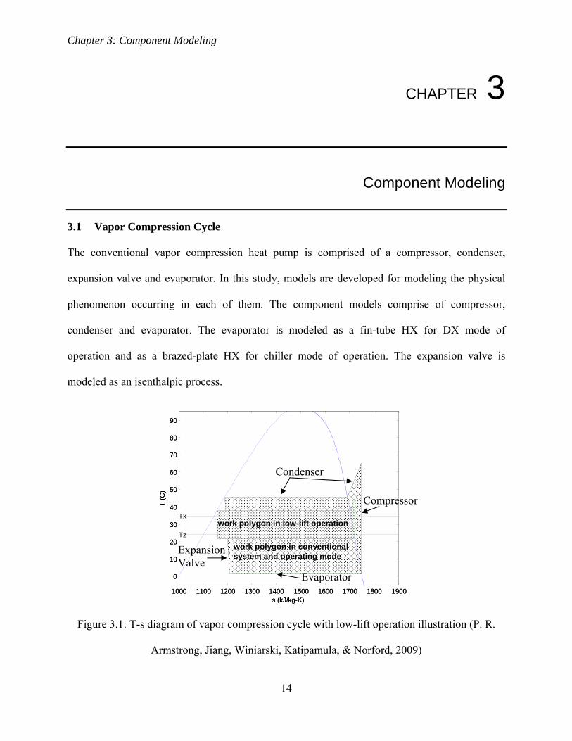
3.1 Vapor Compression Cycle
The conventional vapor compression heat pump is comprised of a compressor, condenser,
expansion valve and evaporator. In this study, models are developed for modeling the physical
phenomenon occurring in each of them. The component models comprise of compressor,
condenser and evaporator. The evaporator is modeled as a fin-tube HX for DX mode of
operation and as a brazed-plate HX for chiller mode of operation. The expansion valve is
modeled as an isenthalpic process.
Figure 3.1: T-s diagram of vapor compression cycle with low-lift operation illustration (P. R.
Armstrong, Jiang, Winiarski, Katipamula, & Norford, 2009)
1000 1100 1200 1300 1400 1500 1600 1700 1800 1900
0
10
20
30
40
50
60
70
80
90
s (kJ/kg-K)
T (C
)
Tz
Tx
1000 1100 1200 1300 1400 1500 1600 1700 1800 1900
0
10
20
30
40
50
60
70
80
90
s (kJ/kg-K)
T (C
)
Tz
Txwork polygon in low-lift operation
work polygon in conventional system and operating mode
Compressor
Condenser
Evaporator
Expansion Valve

Chapter 3: Component Modeling
15
Figure 3.1 illustrates the thermodynamic processes that occur in the components of a vapor
compression cycle. It can be observed from Figure 3.1 that during low-lift operation the work
done by the compressor has been reduced significantly while the magnitude of heat transfer
processes that occur inside the condenser and evaporator remains approximately the same. This
result in a significant increase in COP of the system which is illustrated in Figure 4.7 and Figure
4.8 presented in Chapter 4.
3.2 Refrigerant Oil-Mixture Modeling
In a vapor compression system, oil is required to lubricate the moving parts of the compressor.
Due to clearances required for moving of compressor parts, some oil gets carried to the other
parts of the system. The general trend of oil is to reduce the heat transfer and increase the
pressure drop though researchers have found that presence of oil may sometimes enhance the
heat transfer in the two-phase region (Bandarra Filho et al., 2009; Hu et al., 2008). The oil effect
on the system performance is modeled using the property equations available in the literature. It
is shown in (Thome, 2004) that the Equation 3.2.2 is valid for lubricating oils for temperature
range of -18-204°C and specific gravity2 range of 0.75-1.05. The specific gravity of POE oil for
Viscosity Grade (VG) 22 to VG68 is in the range of 0.98-0.995 at 20°C (“Harp Lubricants –
Technical Data Sheet Harp Polyol Ester Oils,”). The property equations found in the literature
have been developed for refrigerant oil POE/VG68 properties which are given in Equations
3.2.1-3.2.5 (Wei, Ding, Hu, & K. Wang, 2008):
2 Specific gravity is defined as ratio of density of a substance to the density of reference substance such as water.

Chapter 3: Component Modeling
16
ρ 0.97386 6.91673e 4 T 273 /1e3 (3.2.1)
cp 4.1860.388 0.00045 1.8 T 273 32
ρ998.5
. (3.2.2)
k .1172ρ
998.51 0.0054 T 273 (3.2.3)
μ 1062.075 expT 273
32.29 4.90664 1e ρ (3.2.4)
σ 29 0.4 T 273 1e (3.2.5)
The oil is miscible with the refrigerant in liquid phase only. The nominal oil concentration is
therefore specified based on oil mass fraction at the condenser outlet as given by Equation 3.2.6:
ωoilmoil
mrefliq moil (3.2.6)
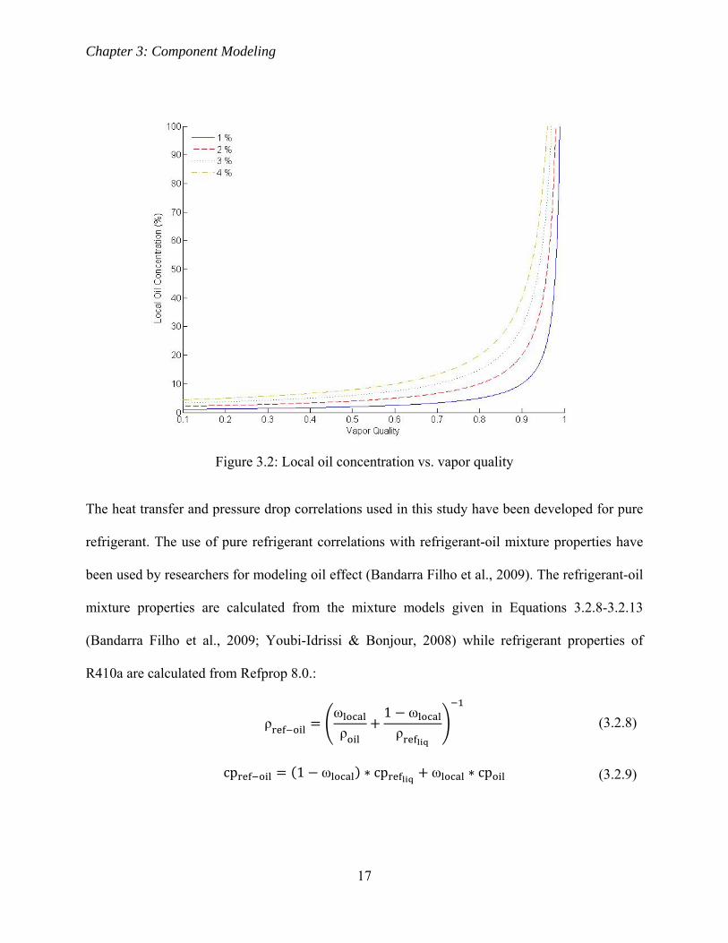
However, when the refrigerant is in two-phase, the nominal oil concentration doesn’t represent
the true oil concentration of refrigerant-oil mixture. The local oil concentration of refrigerant-oil
mixture increases with increasing vapor quality (Wei et al., 2008). The local oil concentration
can be obtained from conservation of mass and is given in Equation 3.2.7:
ωω
1 x (3.2.7)
It is mentioned in (Bandarra Filho et al., 2009) that the vapor quality at the exit of the evaporator
is always less than one because of miscibility of oil with refrigerant. Therefore, refrigerant
properties at the evaporator outlet are always evaluated at saturated pressure and vapor quality of
1-ω . Figure 3.2 illustrates the variation in local oil concentration in the two-phase region.
Chapter 3: Component Modeling
17
Figure 3.2: Local oil concentration vs. vapor quality
The heat transfer and pressure drop correlations used in this study have been developed for pure
refrigerant. The use of pure refrigerant correlations with refrigerant-oil mixture properties have
been used by researchers for modeling oil effect (Bandarra Filho et al., 2009). The refrigerant-oil
mixture properties are calculated from the mixture models given in Equations 3.2.8-3.2.13
(Bandarra Filho et al., 2009; Youbi-Idrissi & Bonjour, 2008) while refrigerant properties of
R410a are calculated from Refprop 8.0.:
ρωρ
1 ωρ
(3.2.8)
cp 1 ω cp ω cp (3.2.9)

Chapter 3: Component Modeling
18
k k 1 ω k ω 0.72 k k
1 ω ω (3.2.10)
μ μ ω μω (3.2.11)
σ σ σ σ ω . (3.2.12)
h h 1 x ω ω hoil x hrefg (3.2.13)
The refrigerant passes through an oil accumulator before entering the compressor as shown in
Figure 4.1. Therefore, enthalpies at the compressor outlet and inlet are calculated using Equation
3.2.14 to account for effect of oil.
href oil h ω h (3.2.14)
Due to presence of oil, the saturation temperature of the refrigerant-oil mixture deviates from
that of the pure refrigerant. Therefore, use of saturation temperature for calculation of two-phase
heat transfer is not correct. In (Bandarra Filho et al., 2009), a bulb temperature is instead
suggested for calculation of two-phase heat transfer. The coefficients of the Equation 3.2.16 and
Equation 3.2.17 are taken from (Bandarra Filho et al., 2009). The coefficients a and b are
specific to a refrigerant and are calculated using the method given in (Thome, 2004). Equation
3.2.15 is used for calculation of bulb temperature given as:
TA
ln P B (3.2.15)
where,
A 182.5 ω 724.2 ω 3868 ω 5268.9 ω (3.2.16)
B b 0.722 ω 2.391 ω 13.779 ω 17.066 ω (3.2.17)

Chapter 3: Component Modeling
19
Figure 3.3: Difference between T and T of pure refrigerant for different T vs. ω
Figure 3.3 represents the difference between saturation temperature of refrigerant-oil mixture and
pure refrigerant. The effect of oil on the mixture’s saturation temperature becomes profound for
high local oil concentration which occurs in high vapor quality region. It is suggested in
(Bandarra Filho et al., 2009), that the mixture properties can be used to calculate heat transfer
coefficient in two-phase flow using the correlations developed for pure refrigerants. However,
for calculation of pressure drop, an adjustment to the friction factor correlations for two-phase
flow is suggested for the model of Moreno et al. (Moreno Quibén & Thome, 2007a). The
adjustment is given in Equation 3.2.18:
dPdx
dPdx
μμ
. ω
(3.2.18)

Chapter 3: Component Modeling
20
It is suggested by Thome that at high vapor qualities i.e. vapor quality greater than 0.9 or when
dryout occurs in the evaporator, the local oil concentration can be taken as zero in the calculation
of heat transfer and pressure drop (Thome, 2011). The oil concentration is taken as 1% of total
refrigerant mass flow in this study which is typical of small hermetic compressors (“Hermetic
Compressors,” 2011). The effect of oil concentration assumption on the vapor compression cycle
components is presented in Chapter 5.
3.3 Compressor
In this study, a semi-empirical model of compressor volumetric efficiency and mass flow rate is
used to estimate the compressor power for given discharge and suction temperatures as presented
in (Zakula, 2010). The thermodynamic power is then converted to compressor electrical power
using the modified model of Jähnig et al. (Jähnig, Reindl, & Klein, 2000) as presented in
(Zakula, 2010).
Equation 3.3.1 describes the compression process:
P ν P ν (3.3.1)
where, ‘n’ is the polytropic exponent which depends on the type of process. Equation 3.3.2 gives
the ‘n’ for a real gas undergoing isentropic compression:
n lnPP / ln
ρρ
(3.3.2)
A compressor in real life doesn’t compress all of the volume that is taken in from the suction side
due to factors such as the clearance volume, back leakage through valves and out of the
compression chamber, pressure loss in the valves mainly suction valve (Jähnig et al., 2000) and

Chapter 3: Component Modeling
21
heat transfer between suction and discharge side which changes with compressor speed. The
mass flow rate through the compressor with no leakage can therefore be described through
Equation 3.3.3:
m C f ρ η (3.3.3)
where, the constant C in Equation 3.3.3 represents the effective swept volume of compressor
and‘ ’ is the compressor speed. Equation 3.3.4 defines the volumetric efficiency η as:
η 1 CPP
/
1 (3.3.4)
where, the constant C represents the clearance volume fraction of the compressor. In the mass
flow model given in (Zakula, 2010), the polytropic exponent is taken as the isentropic polytropic
exponent. An adjustment is made to the mass flow rate to account for the back leakage which is
given in Equation 3.3.5:
m C f ρ η C P P ρ (3.3.5)
The constant C in Equation 3.3.5 represents backflow per unit pressure difference. In
(Willingham, 2009), a pressure loss model similar to the one presented in (Jähnig et al., 2000) is
given. It accounts for the pressure loss in valves and its effect on mass flow rate for a given
compressor speed. It also assumes isentropic compression in the compressor. The model is given
in Equations 3.3.6-3.3.9:
P P C ρ f (3.3.6)
P P C ρ f (3.3.7)
Chapter 3: Component Modeling
22
η 1 CPP
/
1 (3.3.8)
m C f ρ η (3.3.9)
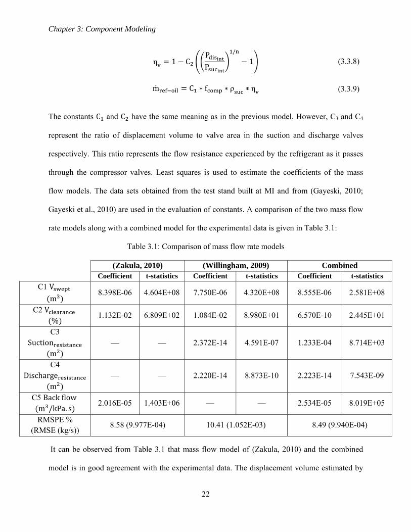
The constants C and C have the same meaning as in the previous model. However, C3 and C4
represent the ratio of displacement volume to valve area in the suction and discharge valves
respectively. This ratio represents the flow resistance experienced by the refrigerant as it passes
through the compressor valves. Least squares is used to estimate the coefficients of the mass
flow models. The data sets obtained from the test stand built at MI and from (Gayeski, 2010;
Gayeski et al., 2010) are used in the evaluation of constants. A comparison of the two mass flow
rate models along with a combined model for the experimental data is given in Table 3.1:
Table 3.1: Comparison of mass flow rate models
(Zakula, 2010) (Willingham, 2009) Combined Coefficient t-statistics Coefficient t-statistics Coefficient t-statistics
C1 V m
8.398E-06 4.604E+08 7.750E-06 4.320E+08 8.555E-06 2.581E+08
C2 V %
1.132E-02 6.809E+02 1.084E-02 8.980E+01 6.570E-10 2.445E+01
C3 Suction
m — — 2.372E-14 4.591E-07 1.233E-04 8.714E+03
C4 Discharge
m — — 2.220E-14 8.873E-10 2.223E-14 7.543E-09
C5 Back flow m /kPa. s
2.016E-05 1.403E+06 — — 2.534E-05 8.019E+05
RMSPE % (RMSE (kg/s))
8.58 (9.977E-04) 10.41 (1.052E-03) 8.49 (9.940E-04)
It can be observed from Table 3.1 that mass flow model of (Zakula, 2010) and the combined
model is in good agreement with the experimental data. The displacement volume estimated by
Chapter 3: Component Modeling
23
the least squares is close to actual displacement volume obtained from the manufacturer which is
9.2e-6m3. The flow resistance coefficients for both suction and discharge valves for the model of
(Willingham, 2009) are almost negligible. However, the flow resistance coefficient for suction
valve in the combined model is significant. F-test is performed to assess the combined model
significance as compared to model of (Zakula, 2010). The F-statistics value was 0.965 and its
significance was computed to be 0.382 which is greater than 0.05. Therefore, mass flow model
of (Zakula, 2010) is used in the compressor model.
A model for calculation of thermodynamic compressor power is suggested in (Jähnig et al.,
2000) to account for the electrical-mechanical conversion and mechanical losses in the
compressor. In (Zakula, 2010), modification is made to the model in which η is taken as a
function of pressure ratio instead of suction pressure. It is given in Equations 3.3.10-3.3.11:
Compressor Power η mn
n 1Pρ
PP 1 (3.3.10)
η C C exp CPP (3.3.11)
Least squares is used to estimate the coefficients for the power model along with the mass model
with the actual displacement volume specified. The coefficients and RMSE predicted by the
model for the experimental data are given in Table 3.2:
Chapter 3: Component Modeling
24
Table 3.2: Coefficients and accuracy of mass and power models
C1 V m 9.200E-06
C2 V % 1.156E-01
C5 Back flow m /kPa. s 1.524E-05
C6 -9.001E-02
C7 1.054E+00
C8 -1.592E-01
RMSPE % (RMSE (kg/s)) 13.16 (1.745E-03)
RMSPE % (RMSE (kW)) 5.24 (1.897E-02)
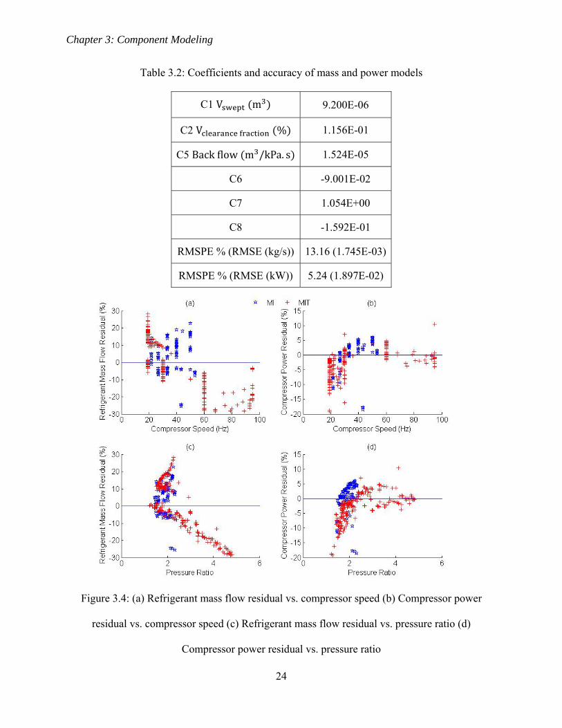
Figure 3.4: (a) Refrigerant mass flow residual vs. compressor speed (b) Compressor power
residual vs. compressor speed (c) Refrigerant mass flow residual vs. pressure ratio (d)
Compressor power residual vs. pressure ratio

Chapter 3: Component Modeling
25
Figure 3.4 shows the residuals of the power and mass flow model. It can be observed that for low
compressor speeds, the residuals for mass flow rate are within ±15% for majority of data points.
However, the mass flow model doesn’t perform well for high pressure ratios occurring at high
compressor speeds. It can be observed from Figure 3.5 that the combined electrical and
mechanical efficiency of the compressor decreases considerably at high pressure ratios.
Figure 3.5: Illustration of η vs. pressure ratio
Chapter 3: Component Modeling
26
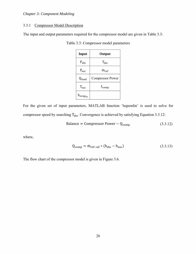
3.3.1 Compressor Model Description
The input and output parameters required for the compressor model are given in Table 3.3:
Table 3.3: Compressor model parameters
Input Output
P T
P m
Q Compressor Power
T f
h
For the given set of input parameters, MATLAB function ‘lsqnonlin’ is used to solve for
compressor speed by searching T . Convergence is achieved by satisfying Equation 3.3.12:
Balance Compressor Power Q (3.3.12)
where,
Q m h h (3.3.13)
The flow chart of the compressor model is given in Figure 3.6.

Chapter 3: Component Modeling
27
Figure 3.6: Compressor model flow chart

Chapter 3: Component Modeling
28
3.4 Fan-Coil Heat Exchanger Model
In this study, the tube-by-tube approach is used to model heat transfer and pressure drop in the
HX. The HX is discretized according to the number of tubes in a loop and then heat transfer and
pressure drop calculations are carried out in a progressive manner. For the transition between
single-phase and two-phase heat transfer, the element length is changed to accurately identify the
location of the transition. For the transition from single-phase to two-phase, the transition
location is calculated to within ±0.01K accuracy while transition from two-phase to single-phase
is calculated to within 1% of vapor quality. The lowest vapor quality in case of condenser is zero
while in case of evaporator the maximum vapor quality is considered as (1-ω ). The ±0.01K
accuracy is considered due to limitation of refrigerant property calculation software.
In (Chen, C.-C. Wang, & S. Y. Lin, 2004; Chen, Wu, Chang, & C.-C. Wang, 2007), it is reported
that the pressure drop in a U-bend is strongly influenced by the curvature of the U-bend
characterized by two times the radius of curvature divided by diameter of tube ‘2R/D’. The
pressure drop for U-bend with 2R/D equals to 3.91 (similar to the Fan-coil HX in our study
whose ‘2R/D’ equals 3.21) and has a circumferential length of 20mm is reported to be 2.5-3.5
times more than the pressure drop encountered in a straight section of 337mm for mass velocities
of 300-400kg/m2/s in the two-phase region (Chen et al., 2004). For our fan-coil HX, a pressure
drop of 2.78kPa is incurred at a vapor quality of 90% for a mass velocity of 288kg/m2/s in a
straight section of 866mm which is 3.2Pa/mm. If we consider three times the pressure drop in the
U-bends of our HX which has circumferential length of 33mm, the pressure drop in the U-bend
is 0.3kPa which is only 10% of the total pressure drop occurring in a length of 866mm. No
appreciable enhancement in the heat transfer coefficient was observed for U-bends with ‘2R/D’

Chapter 3: Component Modeling
29
equals to 2.61 as reported in (Cho & Tae, 2001). Therefore, effect of U-bends on pressure drop
and heat transfer is neglected in the present study.
The fan-coil HX considered in the present study are made up of round copper tubes with stamped
aluminum plain fins joined together by mechanically expanding the tube as explained in (“The
benefits of Aluminum in HVAC&R Heat Exchangers,” 2011). In (Jeong, C. N. Kim, & Youn,
2006), contact resistance between different fan-coil HX is estimated. The different fan-coil HX
consisted on different fin-types, methods of attaching fins to round tubes and whether a
hydrophilic coating was applied to them. It was found that for all the 22 different cases, the
contact resistance comprised of on average around 20% of the total heat transfer resistance which
included the tube resistance, fin resistance and cold and hot-side single-phase water resistance. In
case of two-phase heat transfer, the share of contact resistance in the total heat transfer resistance
will further reduce. Therefore, in this study the effect of contact resistance is neglected.
The effects of physical arrangement of HX circuitry to the air flow are also neglected. The
assumptions that are made for the fan-coil HX model are as follows:
– Uniform ambient/zone temperature
– Uniform air distribution over the HX
– Effect of U-bends on heat transfer and pressure drop is negligible
– Contact resistance between tube and fins is negligible
– Effect of air-side pressure drop on heat transfer is negligible
– HX circuitry arrangement effects on air-side heat transfer are negligible
– Radiation heat transfer effects are negligible
– Condensation or frosting on the outside of tubes is not considered
Chapter 3: Component Modeling
30
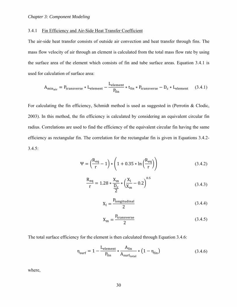
3.4.1 Fin Efficiency and Air-Side Heat Transfer Coefficient
The air-side heat transfer consists of outside air convection and heat transfer through fins. The
mass flow velocity of air through an element is calculated from the total mass flow rate by using
the surface area of the element which consists of fin and tube surface areas. Equation 3.4.1 is
used for calculation of surface area:
A P LL
Pftf P D L (3.4.1)
For calculating the fin efficiency, Schmidt method is used as suggested in (Perrotin & Clodic,
2003). In this method, the fin efficiency is calculated by considering an equivalent circular fin
radius. Correlations are used to find the efficiency of the equivalent circular fin having the same
efficiency as rectangular fin. The correlation for the rectangular fin is given in Equations 3.4.2-
3.4.5:
ΨR
r 1 1 0.35 lnR
r (3.4.2)
R
r 1.28XD2
XX 0.2
.
(3.4.3)
XP
2 (3.4.4)
XP
2 (3.4.5)
The total surface efficiency for the element is then calculated through Equation 3.4.6:
η 1L
Pf
Af
A 1 ηf (3.4.6)
where,

Chapter 3: Component Modeling
31
ηf tanh Ψ mD2 / Ψ m
D2 (3.4.7)
m2 h
kf tf
.
(3.4.8)
A π D L (3.4.9)
A π D L (3.4.10)
Af 2 P Ptf
2 πD2 (3.4.11)
A AfL
PfA (3.4.12)
The air-side heat transfer coefficient is calculated from the correlation of Grey and Webb (Gray
& Webb, 1986) which is given in Equation 3.4.13:
h j1 G cp /Pr (3.4.13)
where,
j 0.14 Re . PP
. Pf
D
.
(3.4.14)
j1 0.991 2.24 Re . tube4
. .
4 tube j (3.4.15)
Chapter 3: Component Modeling
32
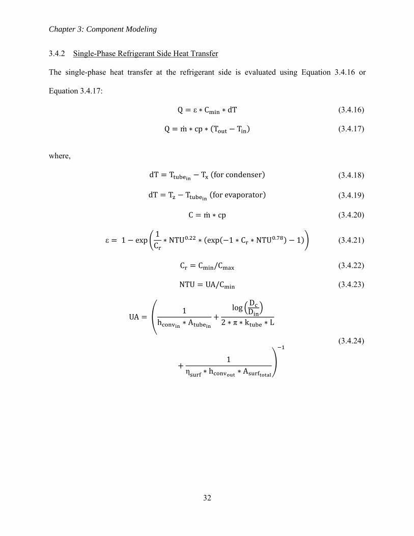
3.4.2 Single-Phase Refrigerant Side Heat Transfer
The single-phase heat transfer at the refrigerant side is evaluated using Equation 3.4.16 or
Equation 3.4.17:
Q ε C dT (3.4.16)
Q m cp T T (3.4.17)
where,
dT T T for condenser (3.4.18)
dT T T for evaporator (3.4.19)
C m cp (3.4.20)
ε 1 exp1C NTU . exp 1 C NTU . 1 (3.4.21)
C C /C (3.4.22)
NTU UA/C (3.4.23)
UA 1
h A
log DD
2 π k L
1η h A
(3.4.24)

Chapter 3: Component Modeling
33
The single-phase heat transfer coefficient for the refrigerant side is calculated based on turbulent
flow correlation. The heat transfer coefficient is calculated from Equation 3.4.25 (Gnielinski,
1976):
hf2 Re 1000 Pr
1 12.7 f2
.Pr 1
kD (3.4.25)
3.4.3 Single-Phase Refrigerant-Side Pressure Drop
The single-phase pressure drop is calculated through the Darcy-Weisbach equation which is
given in Equation 3.4.26:
dpdx 2 f L
GD ρ
(3.4.26)
where, friction factor ‘f’ is calculated using Equation 3.4.27 (Gnielinski, 1976):
f 1.58 log Re 3.28 (3.4.27)
3.4.4 Flow Pattern Map
The flow pattern map developed for refrigerants by (Wojtan, Ursenbacher, & Thome, 2005a) is
used to calculate the heat transfer coefficient and pressure drop for two-phase flow. Figure 3.7
shows the different two-phase flow regimes for a heat flux of 5kW/m2, mass velocity of
300kg/m2/s and saturation temperature of 24°C. It is to be noted that during condensation phase
there is no dryout or mist region.
Chapter 3: Component Modeling
34
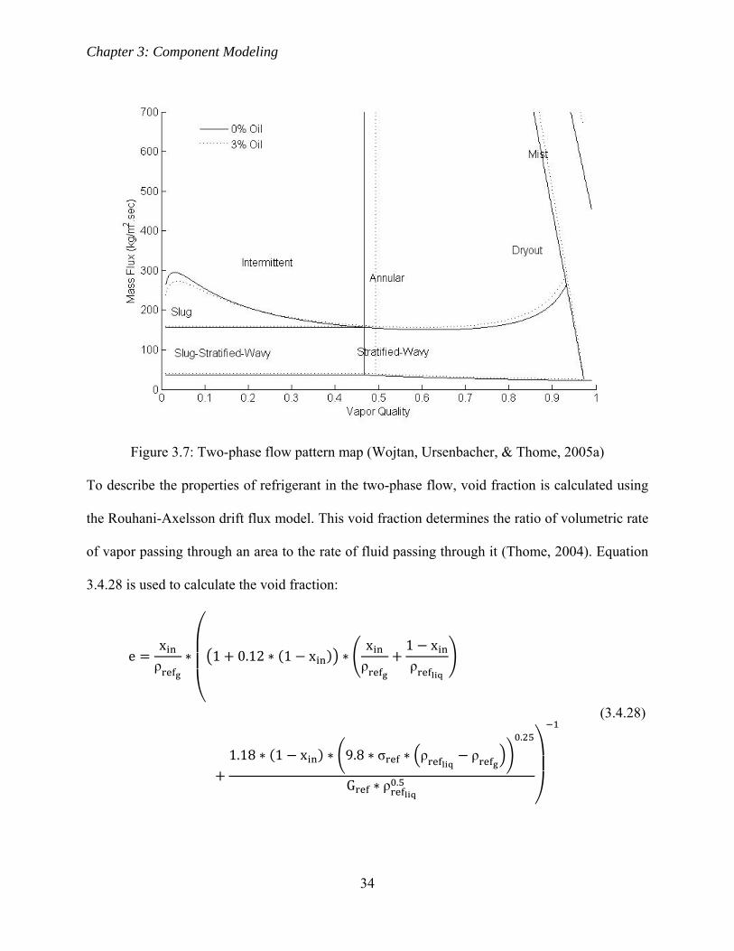
Figure 3.7: Two-phase flow pattern map (Wojtan, Ursenbacher, & Thome, 2005a)
To describe the properties of refrigerant in the two-phase flow, void fraction is calculated using
the Rouhani-Axelsson drift flux model. This void fraction determines the ratio of volumetric rate
of vapor passing through an area to the rate of fluid passing through it (Thome, 2004). Equation
3.4.28 is used to calculate the void fraction:
exρ
1 0.12 1 xxρ
1 xρ
1.18 1 x 9.8 σ ρ ρ.
G ρ .
(3.4.28)
Chapter 3: Component Modeling
35
The liquid and vapor velocities, dimensionless areas, heights and stratification angle are
calculated from Equation 3.4.29-3.4.34:
vGρ
1 x1 e (3.4.29)
vGρ
xe (3.4.30)
A D 1 eπ4 (3.4.31)
A D eπ4 (3.4.32)
h D 0.5 1 cos2π θ
2 (3.4.33)
θ 2π 2
π 1 e3π2 1 2 1 e 1 e e
1200
1 e e 1 2 1 e 1 4 1 e e
(3.4.34)
The boundaries shown in Figure 3.7 are identified using mass fluxes and vapor quality.
Equations 3.4.35-3.4.39 are used to calculate the mass flux boundaries:
G226.3 A D A D ρ ρ ρ μ 9.8
x 1 x π (3.4.35)
If x xIA, G G xIA

Chapter 3: Component Modeling
36
G16 A D 9.8 D ρ ρ
x π 1 2 h D 1.
π25 h D
WeFr 1
.
50 (3.4.36)
where,
WeFr 9.8 Dρ
σ (3.4.37)
G1
0.235 ln0.58x 0.52
Dρ σ
.
9.8 D ρ ρ ρ. ρ
ρ
.qf
q
..
(3.4.38)
If G G , G G ; If G G , G G
G1
0.0058 ln0.61x 0.57
Dρ σ
.
9.8 D ρ ρ ρ. ρ
ρ
.qf
q
..
(3.4.39)
where,
q 0.131 ρ . h 9.8 ρ ρ σ.
(3.4.40)
If G G , G G

Chapter 3: Component Modeling
37
The formula for calculation of intermittent-annular transition vapor quality is given by Equation
3.4.41:
0.2914ρ
ρ. µ
µ1 (3.4.41)
The vapor quality to identify start of dryout region is calculated by Equation 3.4.42:
x 0.58 exp 0.52 0.235 We . Fr .ρ
ρ
.qf
q
. (3.4.42)
where,
We GD
ρ σ (3.4.43)
FrG
9.8 D ρ (3.4.44)
The vapor quality to identify end of dryout region is calculated by Equation 3.4.45:
x 0.61 exp 0.57 5.8 10 We . Fr .ρ
ρ
.qf
q
. (3.4.45)
These equations are then used to identify the flow regimes shown in Figure 3.7 based on the
following:
– Slug
G G xIA
– Slug-Stratified-Wavy
G G xIA and x xIAand G G
Chapter 3: Component Modeling
38
– Stratified-Wavy
x xIA
– Stratified
G G
– Intermittent
G G and x xIA
– Annular
G G and x xIA
– Dryout
G G and x x
– Mist
G G and x x
3.4.5 Two-Phase Refrigerant-Side Heat Transfer
The two-phase heat transfer at the refrigerant side is evaluated using Equation 3.4.16 or Equation
3.4.46:
Q m h x x (3.4.46)
The terms in Equation 3.4.16 for two-phase heat transfer are described in Equations 3.4.47-
3.4.49:
dT T T for condenser (3.4.47)
dT T T for evaporator (3.4.48)

Chapter 3: Component Modeling
39
ε 1 exp NTU (3.4.49)
The heat transfer coefficient for different flow regimes during condensation is calculated using
Equations 3.4.50-3.4.52:
hhf θ 2 π θ h
2 π (3.4.50)
hf 0.655 ρ ρ ρ 9.8 hk
μ D qf (3.4.51)
h 0.003 Re ^0.74 Pr .kδ f
f (3.4.52)
where,
Re 4 G 1 xδ f
1 e μ (3.4.53)
δ fD2
D2
2 A D D2 π θ
.
(3.4.54)
If δ f D /2, δ f D /2
f 1v
v
.
ρ ρ 9.8δ f
σ
.
(3.4.55)
If G G , f f G /G
The heat transfer coefficient for different flow regimes during evaporation excluding dryout and
mist flow regimes is calculated using Equations 3.4.56-3.4.60:
hh θ 2 π θ h
2 π (3.4.56)

Chapter 3: Component Modeling
40
h 0.023 G xD
e μ
.
Pr .kD (3.4.57)
h 0.8 h h (3.4.58)
h 55 P . log10 P . M . qf. (3.4.59)
h 0.0133 Re . Pr .kδ f
(3.4.60)
where,
PP
P (3.4.61)
For R 410a: P 4.9MPa; M 72.585g/mol
The θstrat-wavy for different flow regimes excluding dryout and mist flow regimes is given as:
– Slug
θ 0
– Slug-Stratified-Wavy
θ θxxIA
G GG G
.
– Stratified-Wavy
θ θG G
G G
.
– Stratified
θ θ
– Intermittent
θ 0

Chapter 3: Component Modeling
41
– Annular
θ 0
For the mist flow regime, the heat transfer coefficient is given by Equation 3.4.62:
h 0.0117 ReH. Pr . Y .
kD (3.4.62)
where,
ReH GDμ
xρ
ρ1 x (3.4.63)
Y 1 0.01ρ
ρ1 1 x
.
(3.4.64)
For the dryout flow regime, the heat transfer coefficient is calculated using Equation 3.4.65:
h h xx x
x x
h x h x
(3.4.65)
h x is evaluated from the h applicable to flow regimes other than mist while
h x is evaluated from the h applicable to mist flow regime.

Chapter 3: Component Modeling
42
Figure 3.8: (a) Condensation heat transfer model (b) Evaporation heat transfer model
The heat transfer coefficient variation over the two-phase region along with oil effect on heat
transfer coefficient is illustrated in Figure 3.8 for condensation and evaporation for a heat flux of
5kW/m2, mass velocity of 300kg/m2/s and saturation temperature of 24°C. The heat transfer
coefficients for the dryout and mist flow regimes illustrated in Figure 3.8 are for pure refrigerant.
3.4.6 Two-Phase Refrigerant-Side Pressure Drop
The two-phase pressure drop is calculated using the correlation developed by (Moreno Quibén &
Thome, 2007b). The equations for the different flow regimes are given as:
– Slug
dPdx 2 f L
GD ρ
1e
e xIA
.2 f
L ρvD
ee xIA
.
(3.4.66)

Chapter 3: Component Modeling
43
where,
f 1.58 ln Re 3.28 (3.4.67)
f 0.67δ f
D
.
ρ ρ 9.8δ f
σ
.μ
μ
.
We .
(3.4.68)
δ f D1 e4 π
(3.4.69)
We ρ vDσ
(3.4.70)
– Slug-Stratified-Wavy
dPdx 2 f
LD ρ
G 1e
e xIA
.2 f
L ρvD
ee xIA
.
(3.4.71)
fθ
2 πf 1
θ2 π
f (3.4.72)
f0.079Re . (3.4.73)
Re GDμ
xe (3.4.74)

Chapter 3: Component Modeling
44
– Stratified-Wavy
dPdx 2 f L ρ
vD (3.4.75)
– Stratified
dPdx 2 f L ρ
vD (3.4.76)
fθ2 π
f 1θ2 π
f (3.4.77)
If x xIA
dPdx 2 f
LD ρ
G 1e
e xIA
.2 f
L ρvD
ee xIA
.
(3.4.78)
– Intermittent
dPdx 2 f L
GD ρ
1e
e xIA
.2 f L
ρvD
ee xIA
.
(3.4.79)
– Annular
dPdx 2 f L ρ
vD (3.4.80)
– Mist
dPdx 2 f L
GD ρ
(3.4.81)

Chapter 3: Component Modeling
45
ρ ρ 1 e ρ e (3.4.82)
e
1
1 1 xx
ρρ
(3.4.83)
f0.079Re . (3.4.84)
Re GD
x μ 1 x μ (3.4.85)
– Dryout
dPdx
dPdx x
x xx x
dPdx x
dPdx x
(3.4.86)
P x is evaluated from the P applicable to annular flow regime while P x
is evaluated from the P applicable to mist flow regime.

Chapter 3: Component Modeling
46
Figure 3.9: Pressure drop model
Figure 3.9 illustrates the variation in pressure drop in the two-phase region for evaporation along
with effect of oil for a heat flux of 5kW/m2, mass velocity of 300kg/m2/s and saturation
temperature of 24°C. The pressure drop for the dryout and mist flow regimes illustrated in Figure
3.9 is for pure refrigerant.

Chapter 3: Component Modeling
47
3.4.7 Condenser Model Description
The input and output parameters that are required for the condenser model is given in Table 3.4
and
Table 3.5:
Table 3.4: Condenser model parameters
Input Output
m V
Q T
kW P
T De-superheating zone fraction
P Condensation zone fraction
Condenser details Condenser Effectiveness
System details Estimated P , T , x
Table 3.5: Condenser details required
Tube diameter Tube thermal conductivity
Tube thickness Fin thickness
Tube length Fin width
Tube transversal pitch Fin pitch
Total number of tubes Fin thermal conductivity
Number of stream divisions Condenser height
Number of tubes after streams merge Condenser length
Number of tube rows
Chapter 3: Component Modeling
48
The system details are listed in section 3.6. For the given set of input parameters, V is
searched between its maximum and minimum limits using MATLAB function ‘fmincon’ until
convergence. The maximum and minimum limits in the present study are taken from the
experimental data. The limits are:
Maximum V : 0.67 m3/sec
Minimum V : 0.2 m3/sec
Convergence is achieved by satisfying Equation 3.4.87:
Balance Q Compressor Power sum Q (3.4.87)
A multi-start point search algorithm is used to attain global minimum. In this algorithm,
‘fmincon’ is supplied a set of linearly varying initial points defined between the maximum and
minimum limits. The minimum of the balance from these points is taken as the final solution.
The flow chart of the condenser model is given in Figure 3.10.
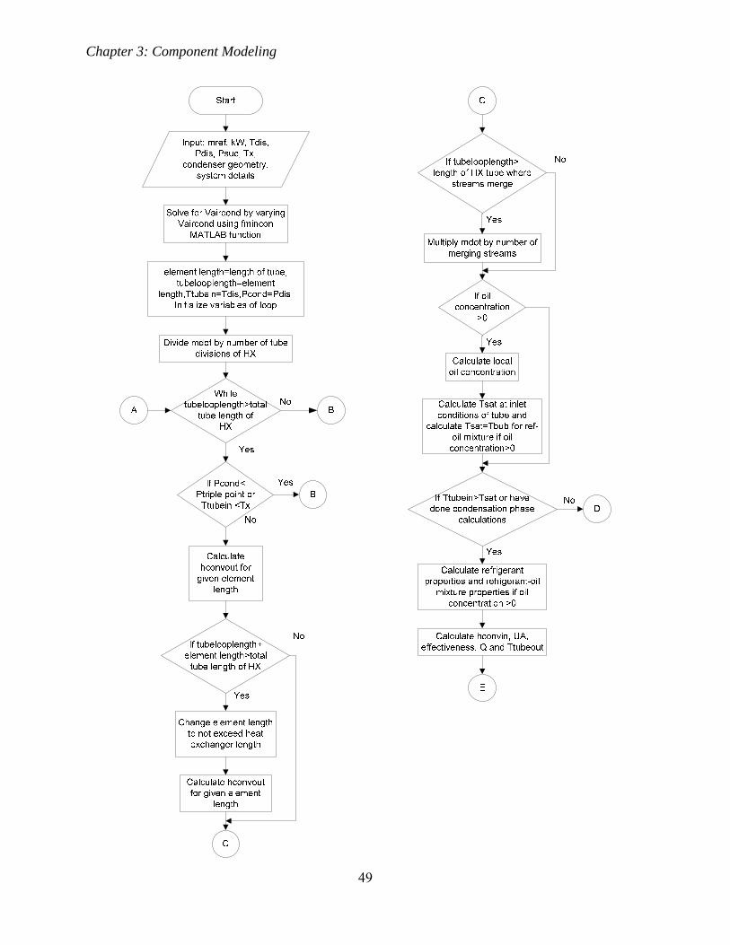
Chapter 3: Component Modeling
49

Chapter 3: Component Modeling
50

Chapter 3: Component Modeling
51

Chapter 3: Component Modeling
52
If dP flag==1
J
If merging of streams have occurred then divided
the dP by number of streams merged
If xin<0.5 then dP of that element is taken as an estimate for dPevap
If condensation has completed
End of condensation loop H
Store Q and Pcond for checking convergence and evaluating total dP of HX
B
Balance=kW+Qload-sum(Q)
Balance=kW+Qload+1-sum(Q)
End of Vaircond solver
A
If Balance<.1kW
K
K
Evaluate hevapin=hcondout at Tcondout and Pcondout
If dP flag==1
Pevapin=Psuc+dPevap estimated
Calculate Tevapin and xinevap at hevapin and Pevapin
End
Cannot solve for given set of input
parameters
Yes
Yes
Yes
Yes Pevapin=Psuc
No No
No
No
No
Output: Tcondout, Pcondout, Vaircond, Pevapin, Tevapin,
xinevap, dPevap,De-superheating fraction, Condensation fraction,
Balance
No
Yes
Figure 3.10: Condenser model flow chart
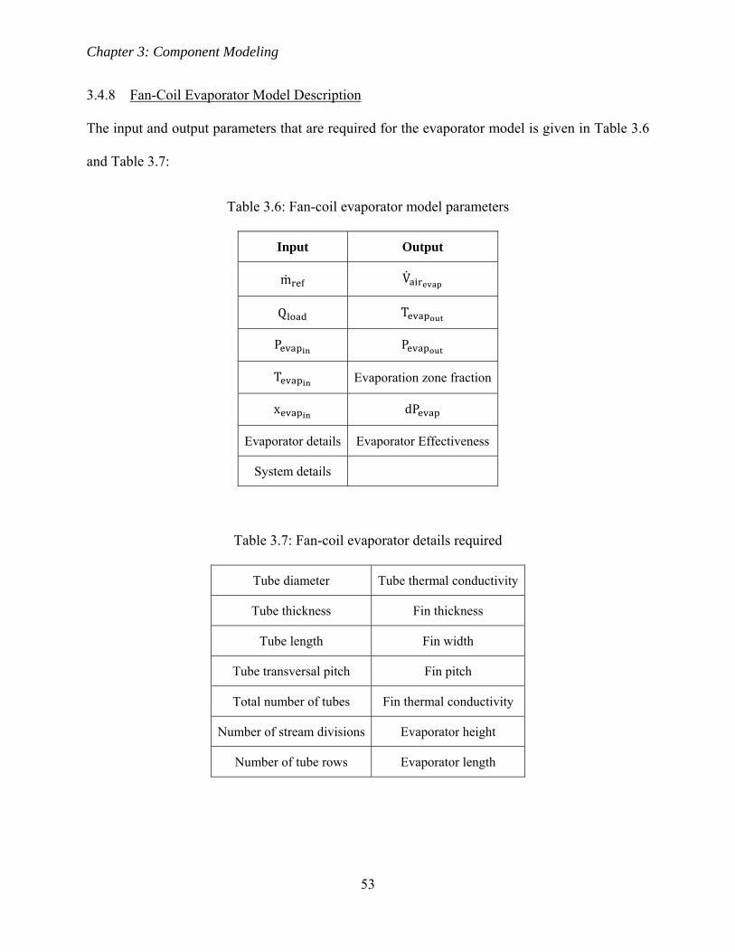
Chapter 3: Component Modeling
53
3.4.8 Fan-Coil Evaporator Model Description
The input and output parameters that are required for the evaporator model is given in Table 3.6
and Table 3.7:
Table 3.6: Fan-coil evaporator model parameters
Input Output
m V
Q T
P P
T Evaporation zone fraction
x dP
Evaporator details Evaporator Effectiveness
System details
Table 3.7: Fan-coil evaporator details required
Tube diameter Tube thermal conductivity
Tube thickness Fin thickness
Tube length Fin width
Tube transversal pitch Fin pitch
Total number of tubes Fin thermal conductivity
Number of stream divisions Evaporator height
Number of tube rows Evaporator length

Chapter 3: Component Modeling
54
The system details are listed in section 3.6. For the given set of input parameters, V is
searched between its maximum and minimum limits using MATLAB function ‘fmincon’ until
convergence. The maximum limit in the present study is taken from the Mitsubishi Mr. Slim
manual of MSZ-A09NA. The limits are:
Maximum V : 0.13 m3/sec
Minimum V : 0.18 m3/sec
Convergence is achieved by satisfying the Equation 3.4.88:
Balance Q sum Q (3.4.88)
A multi-start point search algorithm is used to attain global minimum. In this algorithm,
‘fmincon’ is supplied a set of linearly varying initial points defined between the maximum and
minimum limits. The minimum of the balance from these points is taken as the final solution.
The flow chart of the fan-coil evaporator model is given in Figure 3.11.

Chapter 3: Component Modeling
55

Chapter 3: Component Modeling
56
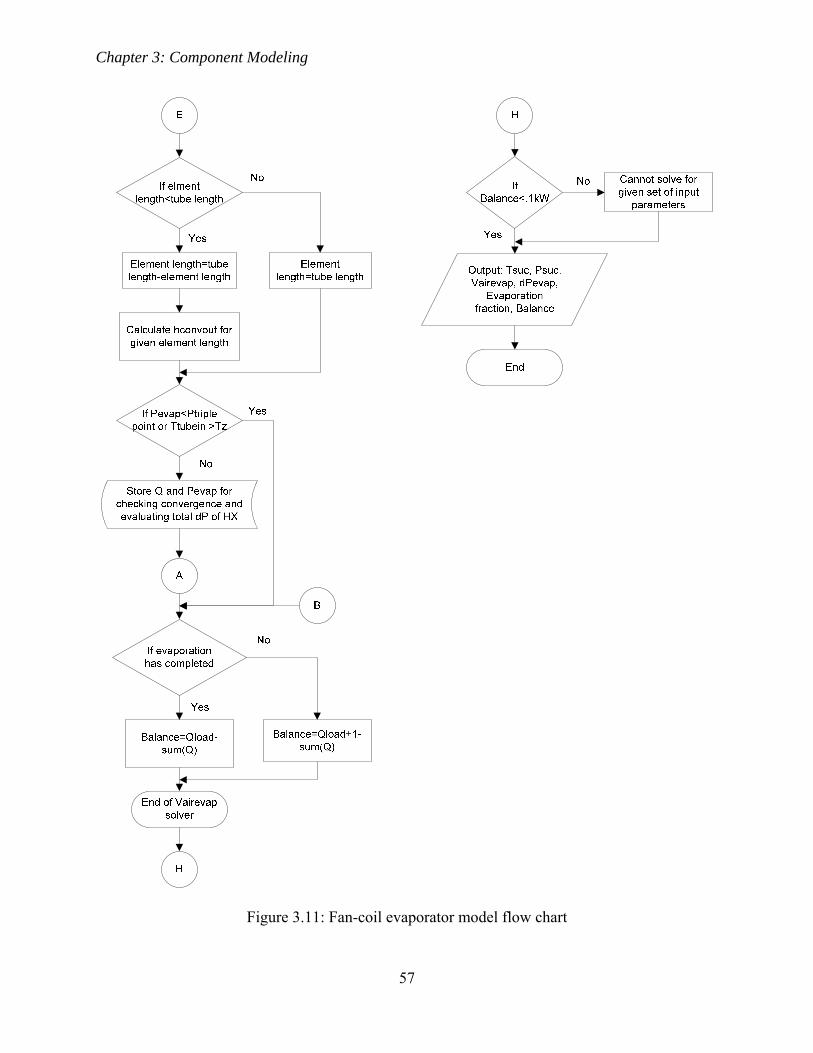
Chapter 3: Component Modeling
57
Figure 3.11: Fan-coil evaporator model flow chart
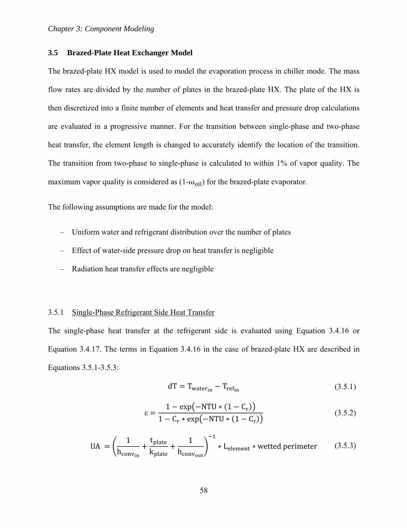
Chapter 3: Component Modeling
58
3.5 Brazed-Plate Heat Exchanger Model
The brazed-plate HX model is used to model the evaporation process in chiller mode. The mass
flow rates are divided by the number of plates in the brazed-plate HX. The plate of the HX is
then discretized into a finite number of elements and heat transfer and pressure drop calculations
are evaluated in a progressive manner. For the transition between single-phase and two-phase
heat transfer, the element length is changed to accurately identify the location of the transition.
The transition from two-phase to single-phase is calculated to within 1% of vapor quality. The
maximum vapor quality is considered as (1-ω ) for the brazed-plate evaporator.
The following assumptions are made for the model:
– Uniform water and refrigerant distribution over the number of plates
– Effect of water-side pressure drop on heat transfer is negligible
– Radiation heat transfer effects are negligible
3.5.1 Single-Phase Refrigerant Side Heat Transfer
The single-phase heat transfer at the refrigerant side is evaluated using Equation 3.4.16 or
Equation 3.4.17. The terms in Equation 3.4.16 in the case of brazed-plate HX are described in
Equations 3.5.1-3.5.3:
dT T T (3.5.1)
ε1 exp NTU 1 C
1 C exp NTU 1 C (3.5.2)
UA 1
htk
1h L wetted perimeter (3.5.3)
Chapter 3: Component Modeling
59
The heat transfer coefficient for single-phase heat transfer is calculated based on Reynolds
number. For Reynolds number less than 1000, the heat transfer coefficient is calculated using
Equations 3.5.4 as (Wanniarachchi, Ratnam, Tilton, & Dutta-Roy, 1995):
h Nu Nu Prμ
μ
. kD (3.5.4)
where,
Nu 3.65 β . . Re . (3.5.5)
Nu 12.6 β . Re (3.5.6)
m 0.646 0.0011 β (3.5.7)
For Reynolds number greater than or equal to 1000, the heat transfer coefficient is calculated
using Equation 3.5.8 (Muley & Manglik, 1999):
h 0.2668 0.006967 β 7.244 10 β
20.78 50.94 41.16 10.51
Re . . π β . Prμ
μ
. kD
(3.5.8)
3.5.2 Single-Phase Refrigerant-Side Pressure Drop
The single-phase pressure drop is calculated through Equation 3.4.26. For Reynolds number less
than 1000, the friction factor ‘f’ is calculated using Equation 3.5.9 (Wanniarachchi et al., 1995):
f f f (3.5.9)
Chapter 3: Component Modeling
60
where,
f 1774 β . Re (3.5.10)
f 46.6 β . Re (3.5.11)
p 0.00423 β 0.0000223 β (3.5.12)
For Reynolds number greater than or equal to 1000, the friction factor ‘f’ is calculated using
Equation 3.5.13 (Muley & Manglik, 1999):
f 2.917 0.1277 β 2.016 10 β
5.474 19.02 18.93 5.341
Re. . π β .
(3.5.13)
The gravitational pressure drop is also added to the frictional pressure drop. The gravitational
pressure drop is given in Equation 3.5.14:
dpdx ρ 9.8 L (3.5.14)
3.5.3 Two-Phase Refrigerant-Side Heat Transfer
The refrigerant side heat transfer in the two-phase region is calculated using Equation 3.4.14 or
Equation 3.4.45. The terms in Equation 3.4.16 for two-phase heat transfer are described in
Equations 3.5.15-3.5.16:
dT T T (3.5.15)
ε 1 exp NTU (3.5.16)
Chapter 3: Component Modeling
61
The heat transfer coefficient for two-phase heat transfer is calculated using Equation 3.5.17
(Hsieh & T. F. Lin, 2003):
h E h S h (3.5.17)
where,
h 55 P . 1 log10 P . M . qf. (3.5.18)
h 0.023 Re Pr . kD (3.5.19)
X1 x
x
. ρρ
. μμ
.
(3.5.20)
E 1 24000qf
G h
.
1.371
X
.
(3.5.21)
S 1 1.15e 6 E Re . (3.5.22)
3.5.4 Two-Phase Refrigerant-Side Pressure Drop
The two-phase pressure drop is calculated using Equation 3.4.26. The friction factor ‘f’ is
calculated using Equation 3.5.23 (Hsieh & T. F. Lin, 2003):
f 23820 Re . (3.5.23)
where,
Re GDμ
(3.5.24)

Chapter 3: Component Modeling
62
G G 1 x xρρ
.
(3.5.25)
The gravitational and acceleration pressure drop are also added to the frictional pressure drop.
The acceleration pressure drop is given in Equation 3.5.26 (Han et al., 2003):
dpdx G
xρ ρ
Gx
ρ ρ (3.5.26)
3.5.5 Port Pressure Drop
The pressure drop at the ports of the brazed-plate HX is given in Equation 3.5.27 (Han et al.,
2003):
dpdx 1.4
mπ4 D
2 ρ
(3.5.27)

Chapter 3: Component Modeling
63
3.5.6 Brazed-Plate Evaporator Model Description
The input and output parameters that are required for the brazed-plate evaporator model is given
in Table 3.8 and
Table 3.9:
Table 3.8: Brazed-plate evaporator model parameters
Input Output
m V
Q T
P P
T Evaporation zone fraction
x dP
Evaporator details Evaporator Effectiveness
System details
Table 3.9: Brazed-plate evaporator details required
Plate length Number of plates
Plate thickness Enlargement factor
Plate width Corrugation pitch
Channel thickness Chevron angle
Port diameters
The system details are listed in section 3.6. For the given set of input parameters, V is
searched between its maximum and minimum limits using MATLAB function ‘fmincon’ until

Chapter 3: Component Modeling
64
convergence. The maximum and minimum limits in the present study are taken from the
experimental data.
The limits are:
Maximum V : 0.28e-3 m3/sec
Minimum V : 0.12e-3 m3/sec
Convergence is achieved by satisfying Equation 3.5.28:
Balance Q sum Q No. of Plates (3.5.28)
A multi-start point search algorithm is used to attain global minimum. In this algorithm,
‘fmincon’ is supplied a set of linearly varying initial points defined between the maximum and
minimum limits. The minimum of the balance from these points is taken as the final solution.
The flow chart of the brazed-plate evaporator model is given in Figure 3.12.

Chapter 3: Component Modeling
65
Start
Input: mref, Qload, Tevapin, Pevap=Pevapin,
xin=xinevap, Twaterin, evaporator geometry,
system details
Solve for Vwaterevap by varying Vwaterevap using fmincon MATLAB function
While platelooplength>
plate length of HX
If platelooplength
+element length>total tube length of
HX
Change element length to not exceed plate
length
No. of elements=10, element length=plate length/no. of elements,
platelooplength=element length,Ttubein=Tevapin, xinlimit=1-oilcon
Initialize variables of loop
Divide mdot by number of plates of HX and
Pevap=Pevap-dpport
C
C
If oil concentration>0
Calculate local oil concentration
Calculate Tsat at inlet conditions of plate element and calculate Tsat=Tbub for
ref-oil mixture if oil concentration>0
If Tplatein<Tsat or have done evaporation phase
calculations
Calculate refrigerant properties and refrigerant-oil
mixture properties if oil concentration >0
Calculate hconvin, UA, effectiveness, Q, Tplateout
and Twaterout
B
D
Yes
Yes
Yes
Yes
No
No
No
If Pevap <Ptriple point or
Tplatein >Twaterin
BYes
No
Calculate dP of element
If dP flag==1
Increase Platelooplength by element length,
Tplatein=Tplateout, Twaterin=Twaterout and proceed to next element
Yes
No
E
A
Calculate hconvout for given element length
Calculate inlet port pressure drop
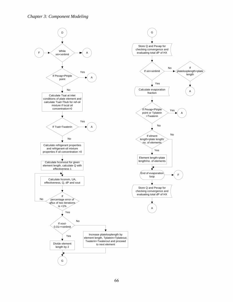
Chapter 3: Component Modeling
66
G
If Pevap<Ptriple point or Tplatein
>TwaterinA
Yes
No
Element length=plate length/no. of elements
Yes
No
If platelooplength>plate
length
A
D
While xin<xinlimit
If Pevap<Ptriple point A
Yes
Calculate Tsat at inlet conditions of plate element and calculate Tsat=Tbub for ref-oil
mixture if local oil concentration>0
If Tsat>Twaterin A
Yes
Calculate refrigerant properties and refrigerant-oil mixture
properties if oil concentration >0
Calculate hconvin, UA, effectiveness, Q, dP and xout
No
No
A
If xout-0.01>=xinlimit
Divide element length by 2
Increase platelooplength by element length, Tplatein=Tplateout, Twaterin=Twaterout and proceed
to next element
No
Yes
G
End of evaporation loop F
Store Q and Pevap for checking convergence and evaluating total dP of HX
A
F
If xin>xinlimit
Store Q and Pevap for checking convergence and evaluating total dP of HX
Calculate evaporation fraction
Yes
No
Calculate hconvout for given element length, calculate Q with
effectiveness 1
If elment length<plate length/
no. of elements
If percentage error of
qflux of two iterations is <1%
No
Yes
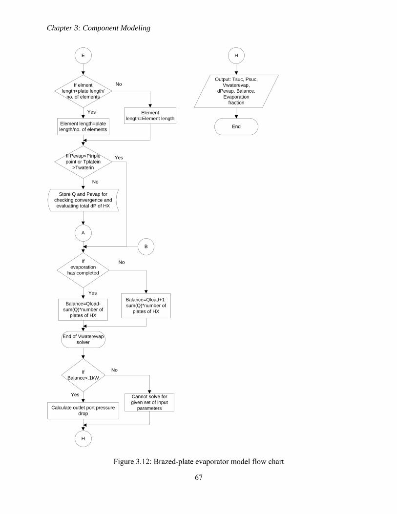
Chapter 3: Component Modeling
67
If elment length<plate length/
no. of elements
Element length=plate length/no. of elements
Element length=Element length
If Pevap<Ptriple point or Tplatein
>Twaterin
A
Yes
Yes
No
No
E
Store Q and Pevap for checking convergence and evaluating total dP of HX
If evaporation
has completed
Balance=Qload-sum(Q)*number of
plates of HX
Balance=Qload+1-sum(Q)*number of
plates of HX
End of Vwaterevap solver
Yes
No
If Balance<.1kW
Calculate outlet port pressure drop
Cannot solve for given set of input
parameters
No
B
End
H
H
Output: Tsuc, Psuc, Vwaterevap,
dPevap, Balance, Evaporation
fraction
Yes
Figure 3.12: Brazed-plate evaporator model flow chart

Chapter 3: Component Modeling
68
3.6 System Model
The system model is developed to estimate the different parameters of the system for a given set
of T , T , Q , P and P .
The system model consists of compressor model, condenser model and evaporator model. The
evaporator model can be either fan-coil HX evaporator model or brazed-plate HX evaporator
model depending on mode of operation. The expansion valve is modeled as an isenthalpic
expansion process. The input and output parameters required for the system model is given in
Table 3.10 and
Table 3.11:
Table 3.10: System model parameters
Input Output
P Component model results
P System power
System details
Table 3.11: System details required
Ambient pressure Maximum temperature of refrigerant
Maximum Pressure of refrigerant
Critical pressure of refrigerant
Triple point pressure of refrigerant
Refrigerant type Oil concentration
Molar mass of refrigerant Fan/pump power curve constants
Minimum temperature of refrigerant Ambient fluid type

Chapter 3: Component Modeling
69
The system power is evaluated using the compressor power from compressor model and
fan/pump power curves for the given amount of volumetric flow rate of air from condenser
model and fan-coil HX evaporator model in case of DX unit operation. For chiller unit operation
volumetric flow rate of water from brazed-plate HX evaporator model is used. System power is
calculated using Equation 3.6.1 or Equation 3.6.2:
For DX unit:
System Power W kW 1e3 fan C V C fan C V C (3.6.1)
For Chiller:
System Power W
kW 1e3 fan C V C pump C V C
pump C
(3.6.2)
The fan or pump power model is derived from the basic fan laws in which the power is described
as a cubic of the volumetric flow rate of air through the fan. Due to electrical and mechanical
conversion losses, the exponent of the power model deviates from the ideal flow-power curve.
The fan-power curve for the condenser is determined through flow hood testing. The evaporator
fan-power curve is obtained using experimental data of power at different speeds and air flow
data at those speeds given in the manufacturer manual. The fan and pump power curve
coefficients and RMSE are given in Table 3.12.

Chapter 3: Component Modeling
70
Table 3.12: Fan and Pump Power Coefficients and RMSE
Condenser Fan DX Evaporator Fan Chiller evaporator pump
C 383.126 431 2.758e+006
C 3.27 1.792 1.493
C — — 18.63
RMSE (W) 0.8595 0.7109 0.6045
For a given set of T , T , Q , P and P , compressor model is called to solve for compressor
output conditions, refrigerant mass flow rate, compressor speed and compressor power. The
output conditions are then supplied to the condenser model to solve for condenser air mass flow
rate and HX outlet conditions. It recalculates the m by calling the compressor model again, as
the evaporator inlet enthalpy is known. If m of the previous iteration and the current iteration
is within 1%, it calls the evaporator model. The evaporator model evaluates the evaporator air or
water mass flow rate and HX outlet conditions. dP is then recalculated as the condenser
model provides an estimate of dP . If dP of the previous and current iteration is within
1%. Recalculation of compressor, condenser and evaporator parameters is done as suction
temperature is known which affects calculation of m as described in Figure 3.6. If suction
temperature the previous and current iteration is within 1%, system power is calculated using
Equation 3.6.1 or Equation 3.6.2 depending on mode of operation. The flow chart of the system
model is given in Figure 3.13.
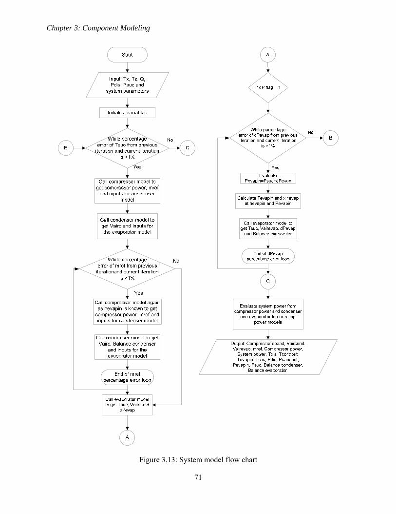
Chapter 3: Component Modeling
71
Figure 3.13: System model flow chart

Chapter 4: Experimental Setup and Instrumentation
72
CHAPTER 4
4 Experimental Setup and Instrumentation
This study is part of the low-lift, radiant-cooling with pre-cooling control project being carried
out at Masdar Institute (MI). A test stand has been built from a Mitsubishi split unit
MUZA09NA-1 for validation of the vapor compression equipment components models
described in Chapter 3. A test chamber has also been built as part of the project to investigate the
savings of low-lift cooling with pre-cooling control over conventional DX units. This chapter
describes the test stand and its instrumentation, the test chamber details and the sensors installed
within, air-tightness of the test chamber, Linear Expansion Valve (LEV) control accuracy, test
stand instrumentation accuracy and experimentation details.
4.1 Test Stand Description
Figure 4.1 describes the instrumentation and different fluid circuits on the test stand. Refrigerant
circuits during DX operation and chiller operation are also shown. Details of the individual
components and sensors installed on the test stand are provided in Appendix A.

Chapter 4: Experimental Setup and Instrumentation
73
Figure 4.1: Test stand component schematic
A refrigerant level indicator is built using two sight glasses and a liquid receiver to observe the
refrigerant liquid level after exit from the condenser. This is required to maintain a certain
refrigerant level head prior to the refrigerant flow meter because the flow meter measures
liquids. If a refrigerant level head is not maintained, flashing of the refrigerant occurs in the flow
meter due to pressure drop across the flow meter. The amount of refrigerant charges for DX
mode and chiller mode of operation used in experimentation are given in Table 4.1:
Table 4.1: Refrigerant charge for DX and Chiller modes of operation
Operation Mode Refrigerant charge
DX 0.907kg (2lb)
Chiller 1.077 (2lb 6oz)
Chapter 4: Experimental Setup and Instrumentation
74
A Y-strainer is installed at the inlet to the brazed-plate HX to prevent fouling of the HX. An
expansion tank is installed in the chilled water circuit to accommodate for water volume changes
with temperature. Four pressure transducers are installed to measure pressures at the inlet and
outlet of the compressor, outlet of condenser and at inlet to the evaporator. The pressure at the
condenser inlet is taken equal to the discharge pressure and the pressure at compressor suction is
taken equal to the outlet of evaporator. In DX mode, the temperature at suction is taken as the
temperature at evaporator outlet. This results in higher residuals for the corresponding
parameters estimated by the models as can be seen in the results presented in Chapter 5.
For determining the accuracy of instrumentation of test stand, a bypass valve is installed in the
chiller circuit to bypass the test chamber. An electric heating element is installed to provide the
heating load and maintain a constant chilled water temperature. The purpose of maintaining a
constant chilled water temperature is to achieve steady state. Evacuation and refilling of
refrigerant is carried out every time switching is made between DX operation and chiller
operation. CR1000 is used to record the data and for controlling the LEV, compressor and
outdoor fan speed. The program for CR1000 is provided in Appendix B.
4.2 Test Chamber Description
The test chamber components, sensors and their locations are described in Figure 4.2. The test
chamber is a modular room with walls made of two painted steel sheets with 6cm fiberglass
insulation between them. The west and south walls are exposed to the surroundings while north
and east walls are the internal walls of the building. A window is located on the south wall with
blinds on the outside. The internal walls and the ceiling are insulated by a 10cm thick

Chapter 4: Experimental Setup and Instrumentation
75
polystyrene insulation to isolate the room from the internal temperatures of the building. The
installation of insulation reduced the heat transfer by 66%. The calculations are provided in
Appendix C. 5cm thick polystyrene insulation is also installed around the slab and 25cm thick
polystyrene insulation is placed beneath the slab to eliminate end heat transfer losses and isolate
the slab from the ground.
Figure 4.2: Test chamber with instrumentation
Prior to installation of insulation in the test chamber, caulking was carried out to seal the cracks
and crevices of the modular room. Acrylic caulk and spray foam insulation was used to make the
room air-tight. This reduced the infiltration load of the room. This will help in estimating the
savings of low-lift radiant cooling system accurately as the technology only handles sensible
N
E
W
S
Fan
Thermal Loads Representing Electronic Equipment
Humidity Sensor
Tube Lights
Indoor Unit
Thermal Loads Representing Sensible Load of Humans
Window
Polystyrene Insulation
Door Pyranometer
Thermocouples
Chapter 4: Experimental Setup and Instrumentation
76
cooling load. After caulking and installing of the insulation, blower door testing was performed
to quantify the air-tightness of the test chamber. The leakage of the room is identified as 40.9cm2
(±0.3%) Canadian Equivalent Area@10Pa and an Air Change per Hour (ACH) of 1.29@50Pa.
The details of the test are provided in Appendix D.
A total of 20 thermocouples are installed in the test chamber, represented by green spheres in
Figure 4.2, to measure the internal temperature distribution. A 4x3 grid of 12 thermocouples is
installed in the slab at a height of 5cm above the 25cm polystyrene insulation. Two vertical
arrays of three additional thermocouples are installed in the slab at a distance of 2.5cm from each
other at two locations. Two pyranometers are also installed on the exposed walls to measure the
solar radiation falling on them. A humidity sensor is installed in the room for monitoring the
specific humidity and the dew point temperature. The detail of thermocouple locations and test
chamber components is presented in Appendix E.
In addition to the sensors, thermal loads are placed inside the room to simulate an office room.
The thermal loads consists of fluorescent tube lights, thermal de-stratification fan and cloth
covered stands representing human sensible load and thermal load of electronic equipment such
as laptops. The detail of the thermal loads is presented in Table 4.2.

Chapter 4: Experimental Setup and Instrumentation
77
Table 4.2: Test Chamber Thermal Loads Description
Item Description Load (W) Load Density (W/m2)
Fluorescent Tube Lights 6 tube light fixtures with 2 tube lights of 28W in each 336 8.118
Human 4 stands with 60W incandescent bulbs 240 5.798
Electronic Equipment 4 stands with 100W incandescent bulbs 400 9.664
Thermal De-stratification Fan 14inch diameter fan 60 1.450
DX Unit Fan Used in DX operation 15 0.386
Total 1051 25.416
4.3 Experimental Data Set
The experimental data set consists of the data obtained from the test stand built at MI and the test
stands used in (Gayeski, 2010; Gayeski et al., 2010). The data sets of (Gayeski, 2010; Gayeski et
al., 2010) are used because of similar vapor compression system. Their data sets are represented
by “MIT DX” and “MIT Chiller” while the data sets obtained from the test stand at MI are
represented by “MI DX” and “MI Chiller” depending on mode of operation. It is to be noted that
a constant heat load was maintained for data sets “MIT DX” and “MIT Chiller” by using a
resistive heater. However, the heat load on the evaporator varied in the case of “MIT Chiller”
and “MI DX” data sets depending on simulated or real outdoor conditions. The steady state was
assumed to be attained by observing the temperatures and pressures of the system over a period
of 30 minutes after any change in compressor or condenser fan speed in the case of “MIT
Chiller” data set while a duration of 15-20 minutes was used in the case of “MI DX” data set.
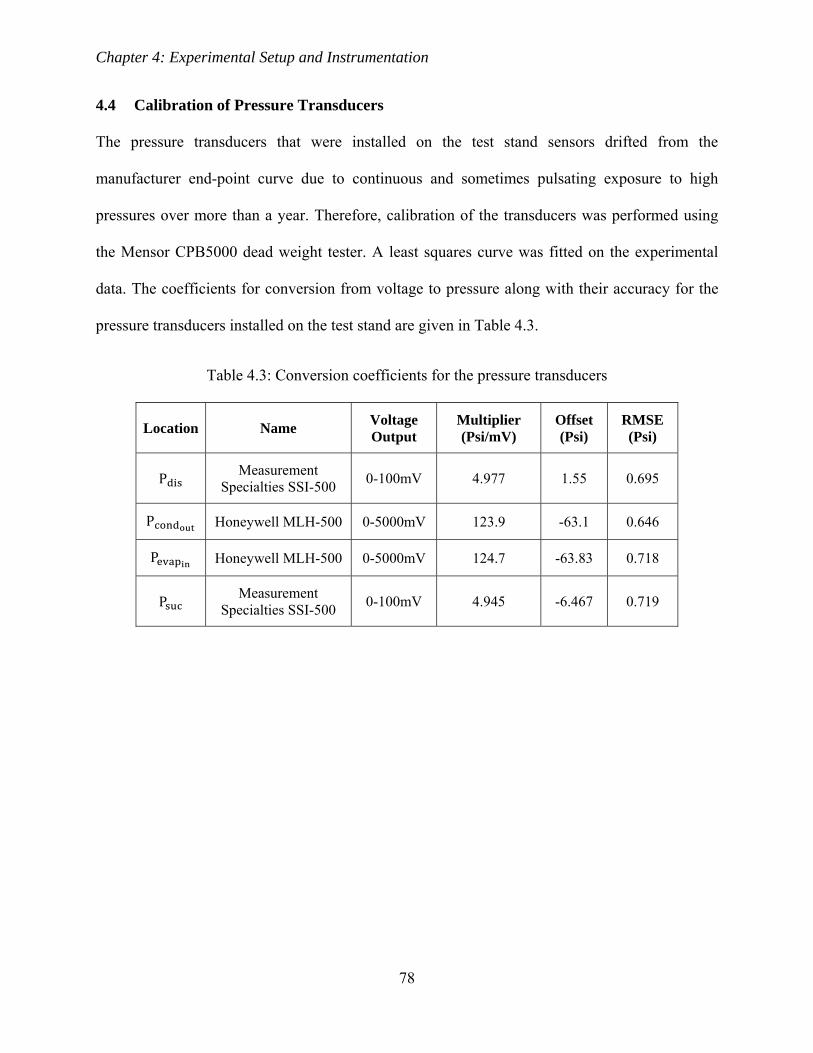
Chapter 4: Experimental Setup and Instrumentation
78
4.4 Calibration of Pressure Transducers
The pressure transducers that were installed on the test stand sensors drifted from the
manufacturer end-point curve due to continuous and sometimes pulsating exposure to high
pressures over more than a year. Therefore, calibration of the transducers was performed using
the Mensor CPB5000 dead weight tester. A least squares curve was fitted on the experimental
data. The coefficients for conversion from voltage to pressure along with their accuracy for the
pressure transducers installed on the test stand are given in Table 4.3.
Table 4.3: Conversion coefficients for the pressure transducers
Location Name Voltage Output
Multiplier (Psi/mV)
Offset (Psi)
RMSE (Psi)
P Measurement Specialties SSI-500 0-100mV 4.977 1.55 0.695
P Honeywell MLH-500 0-5000mV 123.9 -63.1 0.646
P Honeywell MLH-500 0-5000mV 124.7 -63.83 0.718
P Measurement Specialties SSI-500 0-100mV 4.945 -6.467 0.719

Chapter 4: Experimental Setup and Instrumentation
79
Figure 4.3: (a) Pressure residuals before calibration (b) Pressure residuals after calibration
It can be observed from Figure 4.3(a) that the measurement error in the readings of the suction
and evaporator inlet transducers was around 5% or more which increases with increasing
pressure. After calibration these errors have been minimized to within ±1%. The procedure for
calibration is described in Appendix F.
4.5 Condenser Fan Characterization
Flow hood testing on the variable speed condenser fan was performed using TSI air flow hood.
The purpose was to accurately determine the fan curves for air flow and power as a function of
condenser fan speed. An infra-red sensor from Banner Engineering was used to detect each pass
of marked fan blade. Yokogawa 1600 was used to measure three phase power with the flow hood
placed on the outlet of the condenser fan.

Chapter 4: Experimental Setup and Instrumentation
80
Figure 4.4: Condenser fan characterization
A comparison with the fan flow and power data of (Gayeski, 2010) is shown in Figure 4.4. It can
be observed that the air flow for a given condenser fan speed is higher for the condenser fan
installed in the test stand.
4.6 LEV Control Verification
Experimental data was acquired for testing LEV control effectiveness for a range of compressor
speeds. The LEV control is achieved using a 12V stepper motor provided with the outdoor unit.
The stepper motor is controlled by a microcontroller which sends pulses to the motor. The
microcontroller in turn is commanded from the CR1000 using time-based digital signal. It is
estimated that the time for the expansion valve to move from its full open to full close position or
vice versa is 965msec for pulse frequency of 333.33Hz or pulse period of 3msec.
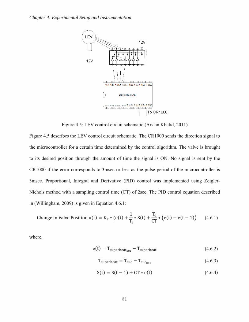
Chapter 4: Experimental Setup and Instrumentation
81
Figure 4.5: LEV control circuit schematic (Arslan Khalid, 2011)
Figure 4.5 describes the LEV control circuit schematic. The CR1000 sends the direction signal to
the microcontroller for a certain time determined by the control algorithm. The valve is brought
to its desired position through the amount of time the signal is ON. No signal is sent by the
CR1000 if the error corresponds to 3msec or less as the pulse period of the microcontroller is
3msec. Proportional, Integral and Derivative (PID) control was implemented using Zeigler-
Nichols method with a sampling control time (CT) of 2sec. The PID control equation described
in (Willingham, 2009) is given in Equation 4.6.1:
Change in Valve Position u t K e t1T S t
TCT e t e t 1 (4.6.1)
where,
e t T T (4.6.2)
T T T (4.6.3)
S t S t 1 CT e t (4.6.4)

Chapter 4: Experimental Setup and Instrumentation
82
The term S(t) is the integrator or sum of errors at time ‘t’. A problem encountered in PI or PID
control is of integral windup. Integral windup occurs when the valve is at its maximum or
minimum position but the error is still non-zero. This causes the integral to keep on summing the
errors. When the sign of the error changes the change in valve position due to summing causes
the valve to start oscillating between its extremes resulting in unstable control. In the current
control algorithm, the integral term is set to zero whenever the valve is at its extremes i.e. the
value of u(t) is 965 or zero. Note that after some hours of operation, the actual position may drift
from the calculated value. Therefore, the valve is closed periodically to eliminate the drift.
Experimentation in chiller mode was conducted to determine the parameters for the PID control
equation. The steady state during the experiment for determining control parameters and testing
the accuracy of LEV control was established by maintaining a constant chilled water outlet
temperature by varying heating load. The heating load is varied using a variable power supply
which controls the power of the electrical resistor. Following the Ziegler-Nicholas method of
tuning, the ultimate gain was found to be 8.5 while the ultimate period was around 90sec. The
coefficients of the PID control equation are given in Table 4.4:
Table 4.4: PID control parameters
Proportional Constant (K ) 5
Integral Time (T ) 45
Derivative Time (T ) 11.25

Chapter 4: Experimental Setup and Instrumentation
83
Figure 4.6: LEV control accuracy with suction superheat as control variable
Figure 4.6 shows the accuracy of maintaining a constant suction superheat for a range of
compressor speeds. We can observe that the control error is less than 0.1°C for majority of the
data points for a suction superheat set point of 1°C.
4.7 DX Mode Operation for Component Models Verification
The test stand was operated under DX mode to acquire data for validation of component models
over a range of compressor speeds, outdoor fan speed and zone temperatures. A superheat of 0K
was maintained through the LEV control within an error of ±0.5K. The error in the superheat for
DX mode was higher because the control time was 5sec which was later changed to 2sec in
chiller mode of operation. The steady state after change of compressor speed was attained by

Chapter 4: Experimental Setup and Instrumentation
84
observing the superheat. The steady state after change of outdoor fan speed was attained by
observing the discharge temperature. The steady discharge temperature was observed to be
within ±0.5K. The steady state time after change of compressor speed was approximately 15-20
minutes. The steady state was achieved within 10-15 minutes after change in outdoor fan speed.
The data from the experiment is provided in Appendix G.
Figure 4.7: System COP plotted against (a) Compressor speed and (b) Pressure ratio
Figure 4.7(a) presents the system COP for a range of compressor speeds. The COP of system
increases considerably at lower speeds. The increase in system COP with pressure ratio as shown
in Figure 4.7(b) follows a more distinct profile than as a function of speed because COP is a
strong function of pressure ratio.
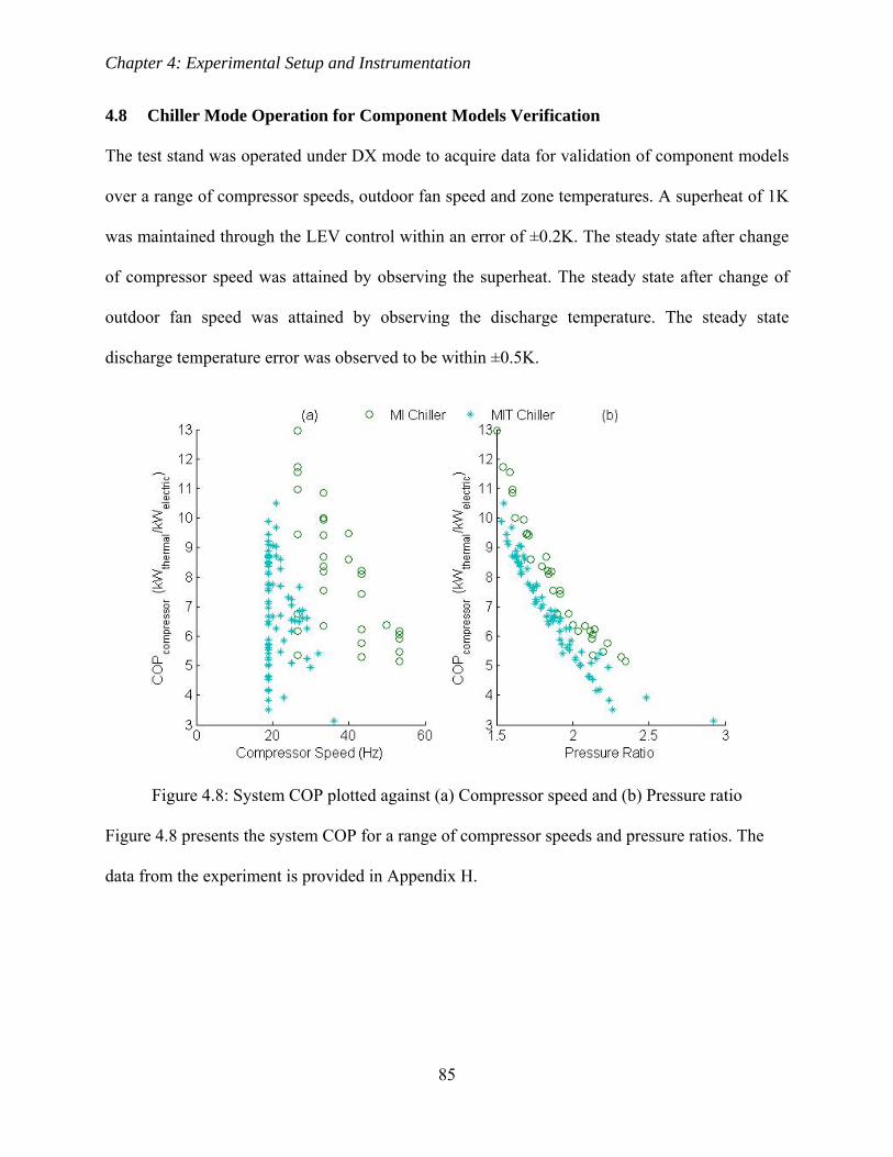
Chapter 4: Experimental Setup and Instrumentation
85
4.8 Chiller Mode Operation for Component Models Verification
The test stand was operated under DX mode to acquire data for validation of component models
over a range of compressor speeds, outdoor fan speed and zone temperatures. A superheat of 1K
was maintained through the LEV control within an error of ±0.2K. The steady state after change
of compressor speed was attained by observing the superheat. The steady state after change of
outdoor fan speed was attained by observing the discharge temperature. The steady state
discharge temperature error was observed to be within ±0.5K.
Figure 4.8: System COP plotted against (a) Compressor speed and (b) Pressure ratio
Figure 4.8 presents the system COP for a range of compressor speeds and pressure ratios. The
data from the experiment is provided in Appendix H.

Chapter 4: Experimental Setup and Instrumentation
86
4.9 Energy Balance Check for the Experimental Data Set
For testing instrumentation accuracy and steady state condition of the system for a given set of
conditions, energy balance was performed on the experimental data set. The energy balance
check was carried out on individual components of the system and on the whole system. Energy
balance check was not performed on the fan-coil evaporator for MI DX data set due to
unavailability of ∆T for the experimental data acquired from the test stand. Energy balance
on condenser for the MI DX data set was not performed due to inaccurate estimation of
condenser fan speed in DX mode of operation. The compressor power shown in the figures is the
three phase electrical compressor power after the variable frequency drive. The mass flow rate of
refrigerant for “MIT DX” data set is calculated from the refrigerant side energy balance on the
evaporator. The oil concentration is taken as 1% in the enthalpy mixture model as mentioned in
(“Hermetic Compressors,” 2011) for small hermetic rotary compressors. The discharge and
suction enthalpies are calculated using Equation 3.2.14 while condenser outlet, evaporator inlet
and evaporator outlet enthalpies are calculated using Equation 3.2.13. The energy balance
equations for the individual components and for the system are given in Equations 4.9.1-4.9.4:
For compressor:
Compressor Power m h h (4.9.1)
For condenser:
m h h m cp @T ,P dT (4.9.2)
For fan-coil evaporator:
m h h m cp @T ,P dT (4.9.3)
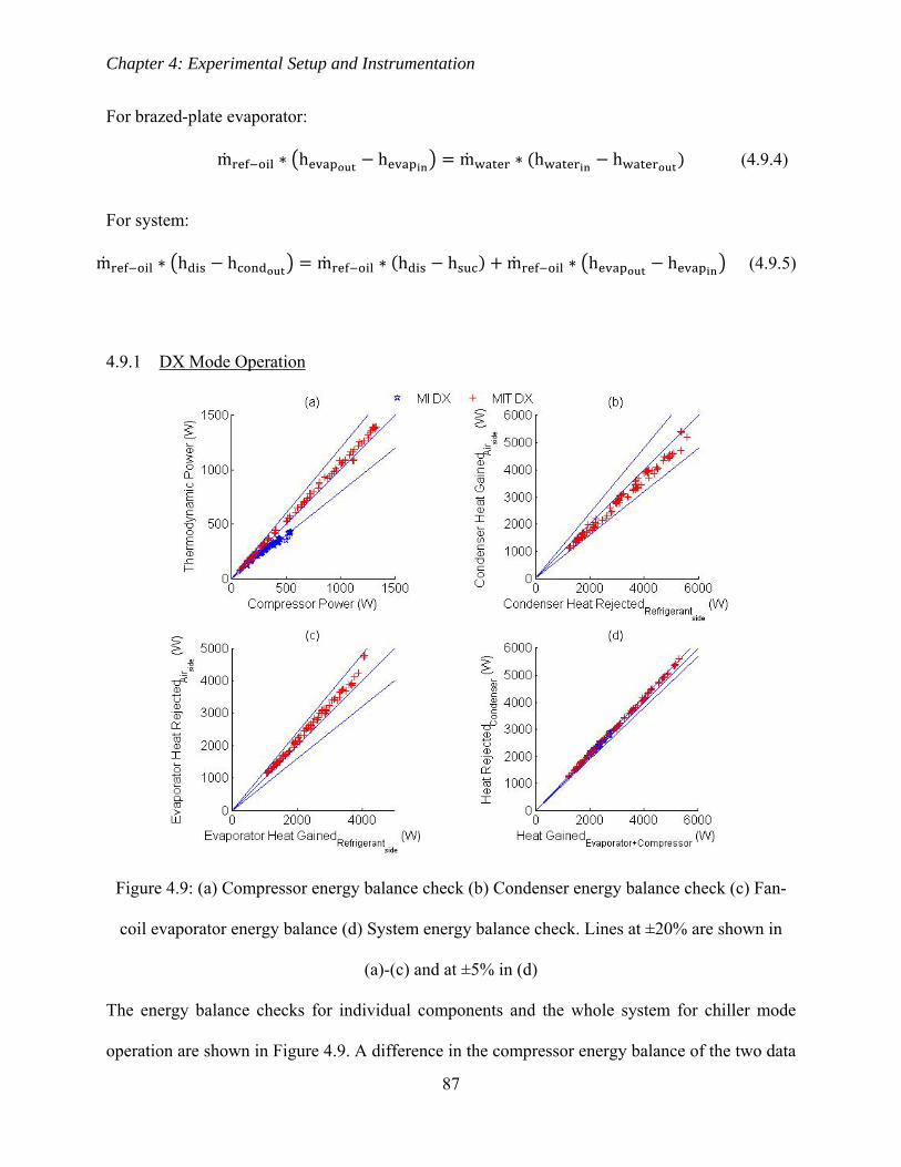
Chapter 4: Experimental Setup and Instrumentation
87
For brazed-plate evaporator:
m h h m h h (4.9.4)
For system:
m h h m h h m h h (4.9.5)
4.9.1 DX Mode Operation
Figure 4.9: (a) Compressor energy balance check (b) Condenser energy balance check (c) Fan-
coil evaporator energy balance (d) System energy balance check. Lines at ±20% are shown in
(a)-(c) and at ±5% in (d)
The energy balance checks for individual components and the whole system for chiller mode
operation are shown in Figure 4.9. A difference in the compressor energy balance of the two data

Chapter 4: Experimental Setup and Instrumentation
88
sets is observed in Figure 4.9(a). This can be because the heat load on the evaporator varied in
“MI DX” data set depending on zone temperature which was influenced by outdoor weather. In
Figure 4.9(b), the heat rejected by the refrigerant is always higher than the heat gain by the air
which can be attributed to error in estimation of air mass flow rate, pressure and temperature
measurements or oil fraction.
In Figure 4.9(c), energy balance on the fan-coil evaporator is shown. The difference between
heat rejected by air and heat gained by refrigerant can be attributed to error in pressure and
temperature measurements. The comparison between heat rejected by fin-tube condenser and the
system heat input presented in Figure 4.9(d) shows that the error in the system energy balance is
within ±5%.
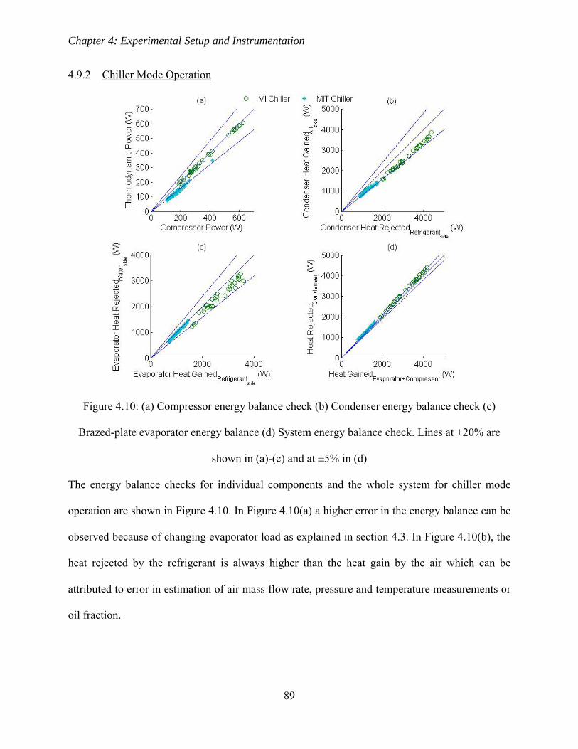
Chapter 4: Experimental Setup and Instrumentation
89
4.9.2 Chiller Mode Operation
Figure 4.10: (a) Compressor energy balance check (b) Condenser energy balance check (c)
Brazed-plate evaporator energy balance (d) System energy balance check. Lines at ±20% are
shown in (a)-(c) and at ±5% in (d)
The energy balance checks for individual components and the whole system for chiller mode
operation are shown in Figure 4.10. In Figure 4.10(a) a higher error in the energy balance can be
observed because of changing evaporator load as explained in section 4.3. In Figure 4.10(b), the
heat rejected by the refrigerant is always higher than the heat gain by the air which can be
attributed to error in estimation of air mass flow rate, pressure and temperature measurements or
oil fraction.

Chapter 4: Experimental Setup and Instrumentation
90
In Figure 4.10(c), energy balance on the brazed-plate evaporator is shown. The difference
between heat rejected by water and heat gained by refrigerant can be attributed to error in
measurement of water mass flow rate. Despite the errors present in the component energy
balance metrics, the system energy balance is obtained to within ±5% as shown in Figure
4.10(d).

Chapter 5: Experimental Validation of Models
91
CHAPTER 5
5 Experimental Validation of Models
5.1 Compressor Model
In Figure 5.1(a) and (b), it can be observed that the accuracy of prediction for compressor speeds
from the model is within ±15% over a range of compressor speeds. The compressor power
prediction accuracy is within ±20% at lower speeds as can be observed in Figure 5.1(d) which is
the area of interest for low-lift operation. However, for higher speeds the power is over-predicted
by the model. This can be because the model doesn’t account for heat transfer between suction
and discharge which becomes significant at high discharge temperatures occurring at high
compressor speeds. Due to heat transfer, the specific volume at suction increase resulting in a
lower mass flow and consequently lower compressor power. However, the current model doesn’t
include the effect of heat transfer on suction resulting in a significant over-prediction of
compressor power as can be seen in Figure 5.1(b) and (d).

Chapter 5: Experimental Validation of Models
92
Figure 5.1: (a) Compressor speed residual vs. compressor speed (b) Compressor speed residual
vs. compressor speed (c) Compressor power residuals vs. compressor power (d) Compressor
power residuals vs. compressor power
Figure 5.2: (a) T residuals vs. compressor speed (b) COP compressor residuals vs. pressure
ratio
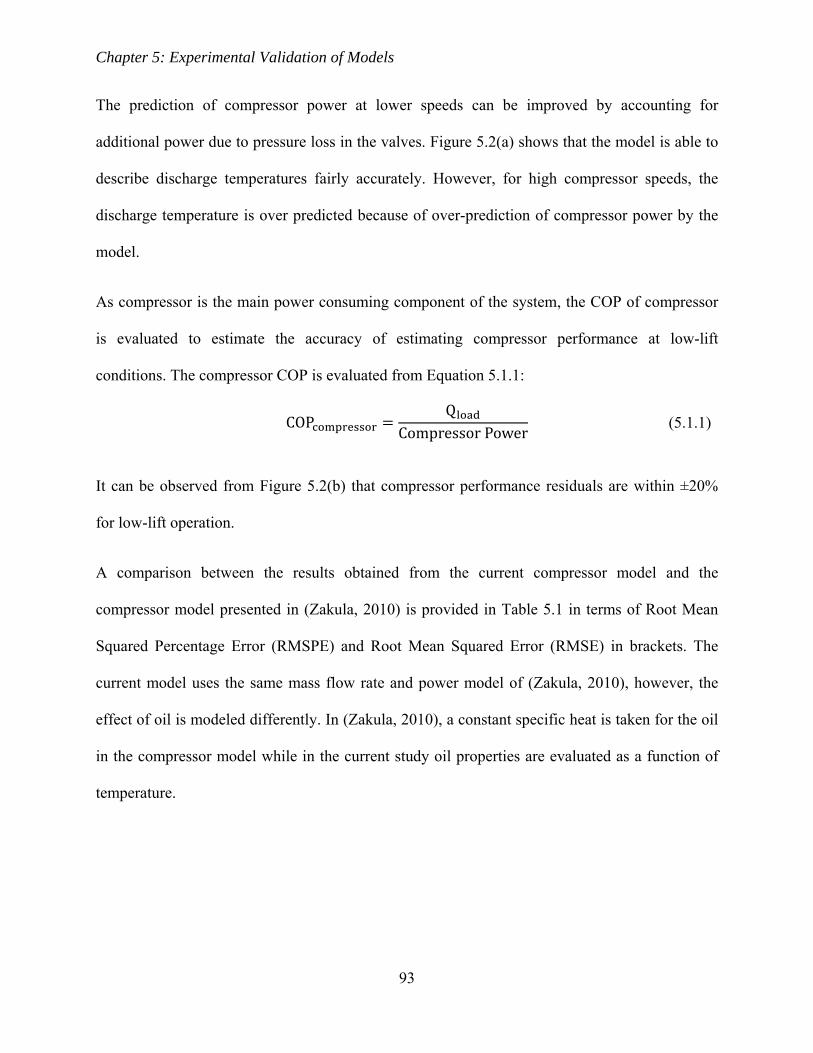
Chapter 5: Experimental Validation of Models
93
The prediction of compressor power at lower speeds can be improved by accounting for
additional power due to pressure loss in the valves. Figure 5.2(a) shows that the model is able to
describe discharge temperatures fairly accurately. However, for high compressor speeds, the
discharge temperature is over predicted because of over-prediction of compressor power by the
model.
As compressor is the main power consuming component of the system, the COP of compressor
is evaluated to estimate the accuracy of estimating compressor performance at low-lift
conditions. The compressor COP is evaluated from Equation 5.1.1:
COPQ
Compressor Power (5.1.1)
It can be observed from Figure 5.2(b) that compressor performance residuals are within ±20%
for low-lift operation.
A comparison between the results obtained from the current compressor model and the
compressor model presented in (Zakula, 2010) is provided in Table 5.1 in terms of Root Mean
Squared Percentage Error (RMSPE) and Root Mean Squared Error (RMSE) in brackets. The
current model uses the same mass flow rate and power model of (Zakula, 2010), however, the
effect of oil is modeled differently. In (Zakula, 2010), a constant specific heat is taken for the oil
in the compressor model while in the current study oil properties are evaluated as a function of
temperature.
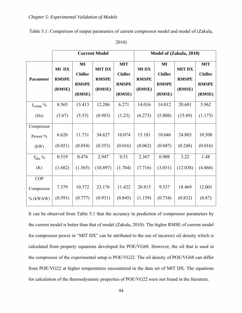
Chapter 5: Experimental Validation of Models
94
Table 5.1: Comparison of output parameters of current compressor model and model of (Zakula,
2010)
Current Model Model of (Zakula, 2010)
Parameter
MI DX
RMSPE
(RMSE)
MI
Chiller
RMSPE
(RMSE)
MIT DX
RMSPE
(RMSE)
MIT
Chiller
RMSPE
(RMSE)
MI DX
RMSPE
(RMSE)
MI
Chiller
RMSPE
(RMSE)
MIT DX
RMSPE
(RMSE)
MIT
Chiller
RMSPE
(RMSE)
f %
(Hz)
8.565
(3.67)
13.413
(5.53)
12.286
(8.983)
6.271
(1.23)
14.016
(6.273)
14.012
(5.808)
20.601
(15.69)
5.962
(1.173)
Compressor
Power %
(kW)
6.626
(0.021)
11.731
(0.054)
34.627
(0.353)
10.074
(0.016)
15.181
(0.062)
10.646
(0.047)
24.803
(0.248)
10.508
(0.016)
T %
(K)
0.519
(1.682)
0.476
(1.565)
2.947
(10.897)
0.51
(1.704)
2.367
(7.716)
0.908
(3.031)
3.22
(12.038)
1.48
(4.866)
COP
Compressor
% (kW/kW)
7.379
(0.591)
10.372
(0.777)
23.176
(0.931)
11.422
(0.845)
20.815
(1.159)
9.537
(0.734)
18.469
(0.832)
12.001
(0.87)
It can be observed from Table 5.1 that the accuracy in prediction of compressor parameters by
the current model is better than that of model (Zakula, 2010). The higher RMSE of current model
for compressor power in “MIT DX” can be attributed to the use of incorrect oil density which is
calculated from property equations developed for POE/VG68. However, the oil that is used in
the compressor of the experimental setup is POE/VG22. The oil density of POE/VG68 can differ
from POE/VG22 at higher temperatures encountered in the data set of MIT DX. The equations
for calculation of the thermodynamic properties of POE/VG22 were not found in the literature.

Chapter 5: Experimental Validation of Models
95
5.2 Condenser Model
Figure 5.3(a) describes the accuracy of prediction of effectiveness by the condenser model for a
given set of P , T , T , m and V . The condenser effectiveness is calculated using
Equation 5.2.1:
εCondenser Heat Rejected
maircond cpair@Tx,PambT T
(5.2.1)
It can be observed that the model predicts the effectiveness within ±5% for the data sets of “MIT
DX” and “MI Chiller” in which a constant heat load was applied. In Figure 5.3(b), the data sets
obtained from the test stand in chiller mode are shown only. This is because the P data
was not present in the DX mode operation in the data set of (Gayeski et al., 2010) and the
location of P transducer in DX mode operation of the MI test stand was after the
refrigerant level indicator which resulted in inaccurate measurement of condenser outlet
pressure. This was later rectified in chiller mode operation. For the data set shown in Figure
5.3(b), the pressure at the condenser outlet is slightly under predicted because the pressure
transducer is not located exactly at the exit of the condenser. For the MI test stand, the transducer
for measuring condenser outlet pressure is located approximately 1.5m after the outlet of the
condenser as shown in Figure 4.1.

Chapter 5: Experimental Validation of Models
96
Figure 5.3: (a) ε residuals vs. measured ε (b) P residuals vs. refrigerant flow rate
(c) T residuals vs. refrigerant flow rate
Figure 5.3(c) shows that the temperature at condenser outlet is under predicted by the model for
majority of data points. In the experimental data obtained from the test stand, this under
prediction increases substantially for some data points in the “MI DX” data set. This can be
attributed to inaccurate estimation of air mass flow rate and non-uniform air flow distribution. It
was found that some air was getting bypassed from the condenser coil due to leaks in the
condenser frame after the coil. This was later rectified and the T residuals decreased as
can be observed in the “MI Chiller” data set. Due to these experimental errors, “MI DX” is not
used for assessment of condenser model performance.

Chapter 5: Experimental Validation of Models
97
Figure 5.4: (a) Heat rejected and (b) dP difference between no oil and 1% oil
Figure 5.4 shows that the condensation heat transfer is decreased when oil is included in the
model for majority of the data points while increasing the pressure drop across the heat
exchanger. A comparison between the results obtained from the current condenser model and the
condenser model presented in (Zakula, 2010) is provided in Table 5.2. The model presented in
(Zakula, 2010) adopts a zone-by-zone approach explained in Chapter 2. Therefore, a
representative heat transfer coefficient and friction factor is calculated for de-superheating,
condensation and sub-cooling region. The model uses film condensation correlation and Pierre’s
correlation for complete evaporation for modeling two-phase heat transfer. For two-phase
pressure drop correlations, an improved version of Pierre’s model developed by Choi, Kazerski
and Domanski are used (Zakula, 2010). The effect of oil on condenser performance is accounted
in calculation of pressure drop. The condenser model presented in (Zakula, 2010) solves for the
condenser inlet pressure and condensation zone fraction to satisfy the energy balance while air
flow rate is varied in the current model to satisfy the energy balance for the given set of input
parameters described in Table 3.4.

Chapter 5: Experimental Validation of Models
98
Table 5.2: Comparison of output parameters of current condenser model and model of (Zakula,
2010)
Current Model Model of (Zakula, 2010)
Parameter
MI
Chiller
RMSPE
(RMSE)
MIT
DX
RMSPE
(RMSE)
MIT
Chiller
RMSPE
(RMSE)
MI
Chiller
RMSPE
(RMSE)
MIT
DX
RMSPE
(RMSE)
MIT
Chiller
RMSPE
(RMSE)
P %
(kPa)
1.934
(47.578) —
0.443
(8.319)
2.376
(62.385) —
3.559
(65.842)
dP %
(kPa)
281.756
(51.557) —
54.309
(8.319)
236.265
(72.91) —
422.866
(65.842)
T %
(K)
0.773
(2.377)
0.745
(2.256)
0.366
(1.097)
0.183
(0.567)
0.316
(0.974)
0.306
(0.92)
dT %
(K)
10.657
(2.377)
8.422
(2.256)
5.097
(1.097)
2.354
(0.567)
2.122
(0.974)
4.368
(0.92)
ε %
(%)
2.025
(0.657)
1.182
(0.289)
6.969
(0.506)
3.033
(0.642)
2.489
(0.396)
0.714
(0.066)
Table 5.2 shows that the prediction accuracy of the current model is better than that of (Zakula,
2010). However, the RMSE for temperature predictions is higher. These errors can be because of
using incorrect oil properties equations such as viscosity, surface tension and thermal
conductivity or oil concentration. It is reported in (Hambraeus, 1995) that a miscible oil of lower
viscosity increases the heat transfer coefficient as compared to a miscible oil of higher viscosity.
In the test stand, VG22 oil is used while only VG68 oil properties were found in literature. The
higher viscosity oils results in an under prediction of condenser outlet temperature for the data
sets of “MIT DX” and “MI Chiller” in which a constant heat load was applied as can be seen in

Chapter 5: Experimental Validation of Models
99
Figure 5.3(c). The effect of oil concentration on condenser output parameters is presented in
Figure 5.10.
5.3 Fan-Coil Evaporator Model
“MIT DX” data set is used for fan-coil evaporator model validation due to unavailability of
evaporator air-side temperature measurements in the data set of “MI DX”. The current model
accurately predicts the heat exchanger effectiveness to within ±10% for a given set of P ,
T , x , T , m and V as shown in Figure 5.5(a).
Figure 5.5: (a) ε residuals vs. measured ε (b) P residuals vs. compressor speed (c)
T residuals vs. compressor speed

Chapter 5: Experimental Validation of Models
100
The evaporator effectiveness is calculated using Equation 5.3.1:
Evaporator EffectivenessEvaporator Heat Gained
mairevap cpair@Tz,PambT T
(5.3.1)
In Figure 5.5(b), the pressure at evaporator outlet is over predicted for majority of data points.
This over prediction increases considerably for data points at and above compressor speed of
60Hz. This can be because of increase in oil concentration which results in a higher pressure
drop. This phenomenon can be observed in Figure 5.5(c) as the suction temperature is under
predicted by the model at higher speeds. It is to be noted that the evaporator outlet pressure and
temperature are measured at compressor suction resulting in higher residuals for these
parameters.
Figure 5.6: (a) Heat rejected and (b) dP difference between no oil and 1% oil
In Figure 5.6(a), no distinct trend of oil is seen on evaporation heat transfer estimation by the
model for low refrigerant flow rates. However, at high refrigerant flow rates an increase in heat
transfer is estimated. The pressure drop was found to increase by inclusion of oil as shown in
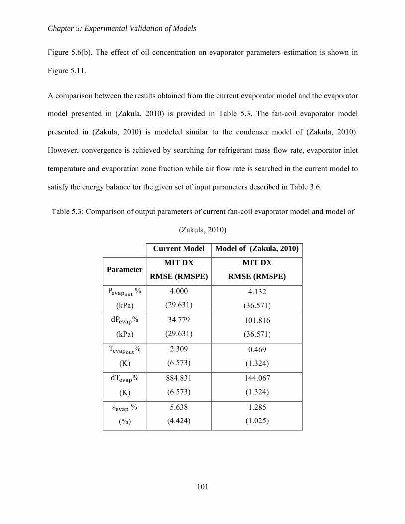
Chapter 5: Experimental Validation of Models
101
Figure 5.6(b). The effect of oil concentration on evaporator parameters estimation is shown in
Figure 5.11.
A comparison between the results obtained from the current evaporator model and the evaporator
model presented in (Zakula, 2010) is provided in Table 5.3. The fan-coil evaporator model
presented in (Zakula, 2010) is modeled similar to the condenser model of (Zakula, 2010).
However, convergence is achieved by searching for refrigerant mass flow rate, evaporator inlet
temperature and evaporation zone fraction while air flow rate is searched in the current model to
satisfy the energy balance for the given set of input parameters described in Table 3.6.
Table 5.3: Comparison of output parameters of current fan-coil evaporator model and model of
(Zakula, 2010)
Current Model Model of (Zakula, 2010)
Parameter MIT DX
RMSE (RMSPE)
MIT DX
RMSE (RMSPE)
P %
(kPa)
4.000
(29.631) 4.132
(36.571)
dP %
(kPa)
34.779
(29.631)
101.816
(36.571)
T %
(K)
2.309
(6.573) 0.469
(1.324)
dT %
(K)
884.831
(6.573)
144.067
(1.324)
ε %
(%)
5.638
(4.424)
1.285
(1.025)
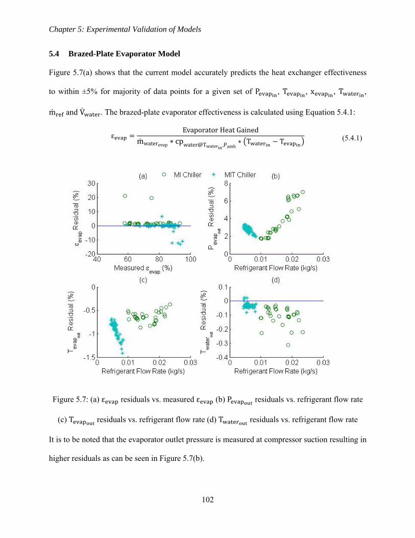
Chapter 5: Experimental Validation of Models
102
5.4 Brazed-Plate Evaporator Model
Figure 5.7(a) shows that the current model accurately predicts the heat exchanger effectiveness
to within ±5% for majority of data points for a given set of P , T , x , T ,
m and V . The brazed-plate evaporator effectiveness is calculated using Equation 5.4.1:
εEvaporator Heat Gained
mwaterevap cpwater@Twaterin,PambT T
(5.4.1)
Figure 5.7: (a) ε residuals vs. measured ε (b) P residuals vs. refrigerant flow rate
(c) T residuals vs. refrigerant flow rate (d) T residuals vs. refrigerant flow rate
It is to be noted that the evaporator outlet pressure is measured at compressor suction resulting in
higher residuals as can be seen in Figure 5.7(b).

Chapter 5: Experimental Validation of Models
103
Figure 5.8: (a) Heat rejected and (b) dP difference between no oil and 1% oil
Figure 5.8 shows that heat transfer decreases with increase in pressure drop after inclusion of oil
in the model. However, the contribution to the decrease in heat transfer is not that significant
while increase in pressure drop is considerable. This can be attributed to the higher area density
found in brazed-plate heat exchangers which eliminates the oil effect of decrease in heat transfer
in the heat exchanger. However, this also increases the pressure drop due to oil in the heat
exchanger.
A comparison between the results obtained from the current brazed-plate evaporator model and
the brazed-plate evaporator model developed by (Zakula, 2011) is provided in Table 5.4. The
brazed-plate evaporator model of (Zakula, 2011) is modeled similar to the fan-coil evaporator
model of (Zakula, 2010). The correlations for single-phase heat transfer and pressure drop are the
same in the current brazed-plate evaporator and the brazed-plate evaporator model of (Zakula,
2011). However, the brazed-plate evaporator model of (Zakula, 2011) uses correlation of Cooper
(Cooper, 1984a) and Choi (Choi, Kedzierski, & Domański, 1999) for two-phase heat transfer and
pressure drop respectively while the current model uses the correlation presented in (Hsieh & T.

Chapter 5: Experimental Validation of Models
104
F. Lin, 2002). Table 5.4 shows that the current brazed-plate evaporator model accurately predicts
the parameters of the heat exchanger as compared to the model of (Zakula, 2011).
Table 5.4: Comparison of output parameters of current brazed-plate evaporator model and model
of (Zakula, 2011)
Current Model Model of (Zakula, 2011)
Parameter
MI Chiller
RMSPE
(RMSE)
MIT Chiller
RMSPE
(RMSE)
MI Chiller
RMSPE (RMSE)
MIT Chiller
RMSPE (RMSE)
P %
(kPa)
4.211
(55.087)
2.828
(28.594)
20.787
(249.967)
3.248
(32.258)
dP %
(kPa)
91.995
(55.087)
95.145
(28.594)
357.61
(249.967)
114.693
(32.258)
T %
(K)
0.784
(2.299)
0.777
(2.208)
0.334
(0.981)
0.325
(0.925)
dT %
(K)
103.243
(2.299)
80.245
(2.208)
63.05
(0.981)
36.003
(0.925)
T %
(K)
0.336
(0.98)
0.172
(0.484)
0.247
(0.722)
0.036
(0.103)
dT %
(K)
50.673
(0.98)
26.665
(0.484)
30.573
(0.722)
6.204
(0.103)
ε %
(%)
0.282
(0.211)
0.129
(0.109)
11.367
(5.536)
3.082
(2.521)
Table 5.4 shows that the prediction accuracy of the current model is better than that of (Zakula,
2010). However, the RMSE for the temperature is slightly higher. This can be because of using
incorrect oil properties equations such as viscosity, surface tension and thermal conductivity
which are for POE/VG68.

Chapter 5: Experimental Validation of Models
105
5.5 Oil Concentration Effect on Vapor Compression Components:
5.5.1 Compressor:
It can be observed from Figure 5.9 that in “MIT DX” data set, the errors in prediction of
compressor performance decreases at higher oil concentration. It is mentioned in (Sarntichartsak
et al., 2006) that oil concentration in variable speed compressor varies with compressor speed.
For a hermetic rotary compressor, the oil concentration varied from 0.5% to 1% for compressor
electrical frequency of 30-50Hz. However, in “MIT DX” data set the compressor electrical
frequency range was 60-300Hz. Therefore, use of oil concentration equation as a function of
speed may reduce the errors encountered in the component models especially for “MIT DX” data
set.
Figure 5.9: Oil concentration effect on (a) Compressor speed (b) Compressor power (c)
Discharge temperature (d) Compressor COP

Chapter 5: Experimental Validation of Models
106
5.5.2 Condenser:
Figure 5.10 illustrates the effect of oil on the prediction of condenser output parameters. It can be
observed from Figure 5.10(c) that an increase in oil concentration increases the effectiveness
error in “MI Chiller” and “MIT DX”. It was shown in Figure 5.4(a) that the heat transfer was
found to decrease after inclusion of oil for majority of data points. Therefore, it can be suggested
that oil tends to enhance condensation heat transfer. However at low refrigerant flow rates, oil
may reduce the heat transfer slightly as can be seen by a decrease in ε RMSE in Figure
5.10(c). The error in condenser outlet pressure estimation is found to increase with oil
concentration in Figure 5.10(a). This discrepancy is because of using VG68 oil properties which
results in a higher pressure drop than measured. However, the effect of this is negligible at low
refrigerant flow rates encountered in data set of “MIT Chiller”.
Figure 5.10: Oil concentration effect on condenser (a) Outlet pressure (b) Outlet temperature and
(c) Effectiveness
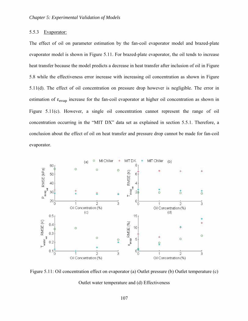
Chapter 5: Experimental Validation of Models
107
5.5.3 Evaporator:
The effect of oil on parameter estimation by the fan-coil evaporator model and brazed-plate
evaporator model is shown in Figure 5.11. For brazed-plate evaporator, the oil tends to increase
heat transfer because the model predicts a decrease in heat transfer after inclusion of oil in Figure
5.8 while the effectiveness error increase with increasing oil concentration as shown in Figure
5.11(d). The effect of oil concentration on pressure drop however is negligible. The error in
estimation of ε increase for the fan-coil evaporator at higher oil concentration as shown in
Figure 5.11(c). However, a single oil concentration cannot represent the range of oil
concentration occurring in the “MIT DX” data set as explained in section 5.5.1. Therefore, a
conclusion about the effect of oil on heat transfer and pressure drop cannot be made for fan-coil
evaporator.
Figure 5.11: Oil concentration effect on evaporator (a) Outlet pressure (b) Outlet temperature (c)
Outlet water temperature and (d) Effectiveness

Chapter 5: Experimental Validation of Models
108
5.6 System Model
Figure 5.12: (a) Compressor speed residual vs. compressor speed (b) Vaircond residual vs. aircond
(c) Vairevap residual vs. Vairevap(d) System COP residuals vs. measured system COP
Figure 5.12 shows the accuracy of prediction of refrigerant and air flow rates by the system
model. The refrigerant flow rate is predicted within an accuracy of ±5%. However, it is under-
predicted for majority of data points. As shown in Figure 5.3(a) that for a given set of input
parameters as described in Table 3.4 and V , the condenser effectiveness is predicted within an
error of ±20%. However, when the solver searches for V to satisfy the condenser energy
balance, a higher V is estimated by the model resulting in over-prediction of V . This over-
prediction increases considerably at low air volumetric flow rates due to under-prediction of
refrigerant mass flow rate and inaccuracy in prediction of compressor power by the compressor
model. This is because the effect of V on heat transfer conductance given in Equation 3.4.24 is
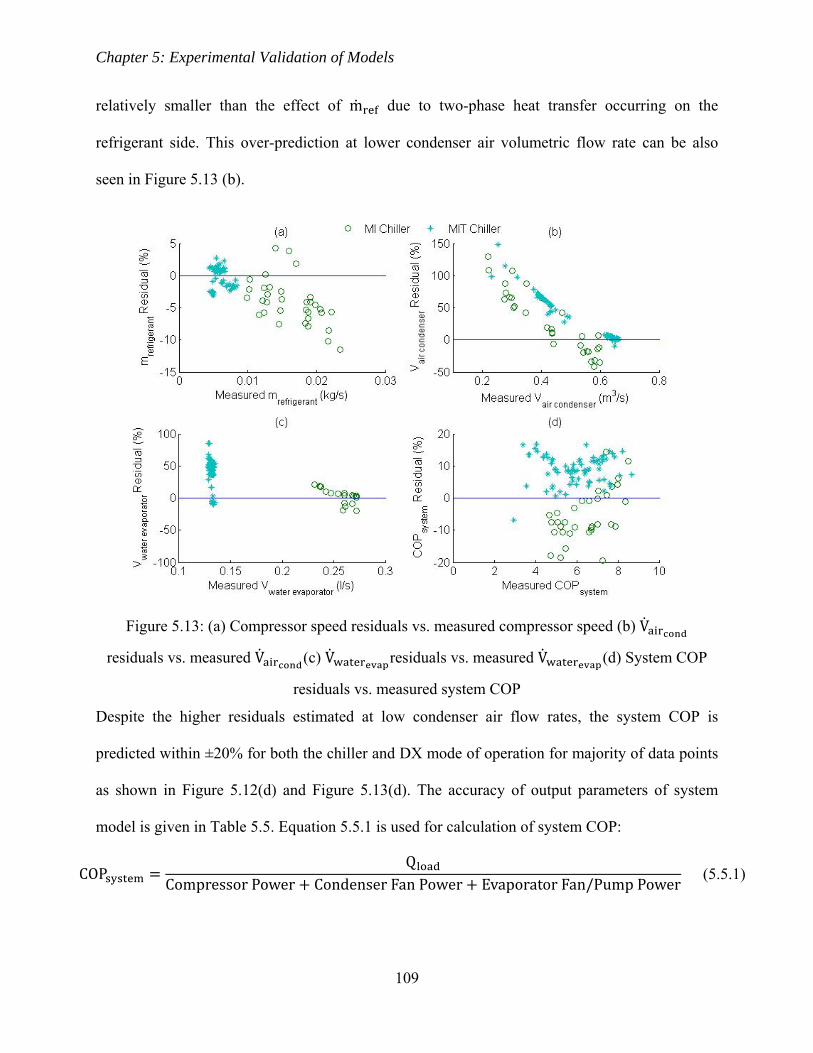
Chapter 5: Experimental Validation of Models
109
relatively smaller than the effect of m due to two-phase heat transfer occurring on the
refrigerant side. This over-prediction at lower condenser air volumetric flow rate can be also
seen in Figure 5.13 (b).
Figure 5.13: (a) Compressor speed residuals vs. measured compressor speed (b) V
residuals vs. measured V (c) V residuals vs. measured V (d) System COP
residuals vs. measured system COP
Despite the higher residuals estimated at low condenser air flow rates, the system COP is
predicted within ±20% for both the chiller and DX mode of operation for majority of data points
as shown in Figure 5.12(d) and Figure 5.13(d). The accuracy of output parameters of system
model is given in Table 5.5. Equation 5.5.1 is used for calculation of system COP:
COPQ
Compressor Power Condenser Fan Power Evaporator Fan/Pump Power (5.5.1)

Chapter 5: Experimental Validation of Models
110
Table 5.5: Output parameters of system model
Parameter MIT DX RMSPE (RMSE)
MI Chiller RMSPE (RMSE)
MIT Chiller RMSPE (RMSE)
f % (Hz)
9.891 (5.384)
9.413 (3.808)
8.703 (1.763)
m % (kg/s)
2.534 (0.0004)
5.414 (0.001)
1.452 (0.00008)
Compressor Power % (kW)
30.223 (0.298)
6.734 (0.027)
12.562 (0.019)
T % (K)
2.413 (8.847)
0.904 (2.98)
2.513 (8.157)
P % (kPa) — 1.062
(25.427) 0.416
(7.979) dP %
(kPa) — 521.883 (25.391)
50.087 (7.972)
T % (K)
0.879 (2.661)
1.678 (5.195)
0.472 (1.427)
dT % (K)
9.672 (2.661)
21.118 (5.201)
6.324 (1.453)
ε % (%)
4.905 (0.008)
0.546 (0.001)
7.791 (0.006)
T % (K)
2.351 (6.677)
0.376 (1.102)
0.783 (2.226)
dT % (K)
747.123 (6.677)
47.09 (1.102)
82.726 (2.226)
T % (K) — 0.142
(0.416) 0.182
(0.512) dT %
(K) — 21.776 (0.43)
27.938 (0.516)
ε % (%)
6.487 (0.052)
14.821 (11.5)
4.166 (3.6)
V % (m3/s)
62.862 (0.153)
58.812 (0.175)
69.304 (0.218)
V % (m3/s)
14.229 (0.021) — —
V % (l/s)
— 10.564 (0.026)
47.814 (0.063)
COP System % 20.913 (0.721)
9.235 (0.586)
10.322 (0.606)

Chapter 5: Experimental Validation of Models
111
5.7 Optimal Performance Map for Control of Compressor Speed and Outdoor Fan Speed
In order to operate the vapor compression equipment at the optimal conditions for pre-cooling
control, curve fitting is performed on the data obtained from optimization presented in (Zakula,
2010). This is because the optimization time for a given set of conditions is very large and it is
impractical to perform the optimization online because of the computational limitations. As
shown in section 5.1-5.4 that the accuracy in prediction of output parameters of the component
models presented in the current study and presented in (Zakula, 2010) is comparable. Therefore,
curves for obtaining the optimum compressor speed and outdoor fan speeds were generated as a
function of T , T and Q from the optimization data of (Zakula, 2010). In the current test stand
speed control is not implemented over evaporator fan or pump. Therefore no curves were
generated for their speed control. The optimization data of (Zakula, 2010) is used for speed
control curves due to very high computational time required by the current models and failure to
successfully use the optimization routines of MATLAB for system model.
Equation 5.7.1 is used to calculate the condenser fan speed from condenser volumetric flow rate.
The constants in Equation 5.7.1 are determined through flow hood experiment explained in
Chapter 4:
Condenser fan speed rpm 1547 V . (5.7.1)
The compressor speed obtained from the system model is converted to electrical frequency by
Equation 5.7.2:
Electrical Speed HzShaft Speed Number of Poles
2 (5.7.2)
Therefore, the shaft speed obtained from the model is multiplied by 3 because the compressor
electric motor is of 6 poles. The equations for the optimal compressor and condenser air flow

Chapter 5: Experimental Validation of Models
112
rate for DX mode and Chiller mode are given by Equation 5.7.3-5.7.6. The coefficients of
Equations 5.7.3-5.7.6 are given in
Table 5.6:
5.7.1 DX Mode
f C C Q C Q T C Q T C Q C TC T C Q T C Q T C Q T C Q
T C T T C Q T T C Q C T
(5.7.3)
rpm C C T C T C Q T C T T C T CQ T C Q T C Q T C T T CQ T C T T C Q T T C Q
(5.7.4)
5.7.2 Chiller Mode
f C C Q C T C Q T C Q T C T T
C Q C T C Q T C Q T C Q TC T T C Q T C T T C Q T TC Q C T C T
(5.7.5)
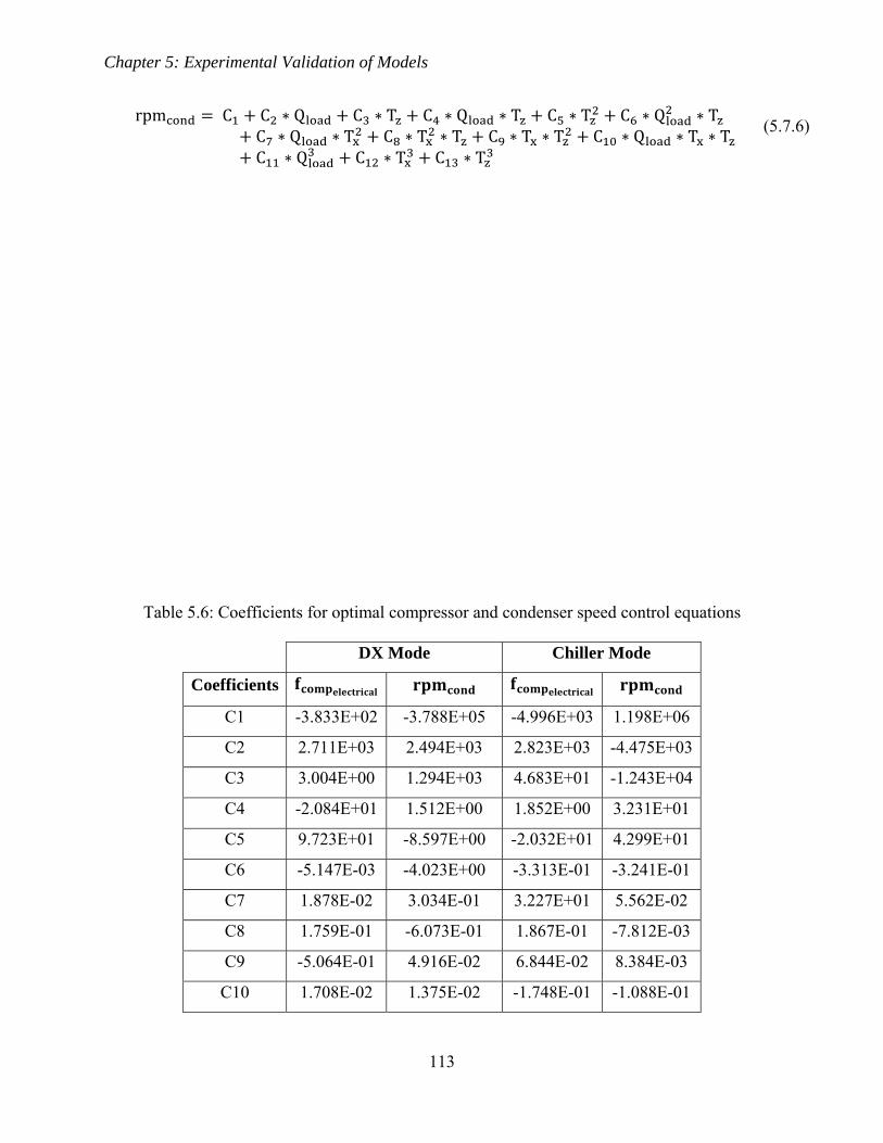
Chapter 5: Experimental Validation of Models
113
rpm C C Q C T C Q T C T C Q TC Q T C T T C T T C Q T TC Q C T C T
(5.7.6)
Table 5.6: Coefficients for optimal compressor and condenser speed control equations
DX Mode Chiller Mode
Coefficients
C1 -3.833E+02 -3.788E+05 -4.996E+03 1.198E+06
C2 2.711E+03 2.494E+03 2.823E+03 -4.475E+03
C3 3.004E+00 1.294E+03 4.683E+01 -1.243E+04
C4 -2.084E+01 1.512E+00 1.852E+00 3.231E+01
C5 9.723E+01 -8.597E+00 -2.032E+01 4.299E+01
C6 -5.147E-03 -4.023E+00 -3.313E-01 -3.241E-01
C7 1.878E-02 3.034E-01 3.227E+01 5.562E-02
C8 1.759E-01 -6.073E-01 1.867E-01 -7.812E-03
C9 -5.064E-01 4.916E-02 6.844E-02 8.384E-03
C10 1.708E-02 1.375E-02 -1.748E-01 -1.088E-01

Chapter 5: Experimental Validation of Models
114
C11 5.777E-02 5.166E-02 1.224E-02 1.238E+01
C12 4.269E-05 2.551E-04 -6.687E-04 2.429E-03
C13 -4.503E-02 -1.011E-01 4.902E-02 -5.256E-02
C14 1.277E+00 1.215E+01 1.291E-03 —
C15 -7.405E-05 — -3.070E-02 —
C16 — — 8.150E-02 —
C17 — — 2.126E-04 —
C18 — — -6.889E-04 —
RMSE 1.0433 (Hz) 11.1095 (rpm) 0.3256 (Hz) 11.71 (rpm)
Figure 5.14: Illustration of optimal compressor speeds for DX and chiller mode operation for a
given Q , T and T
Figure 5.14 describes the optimal compressor speeds for a given set of Q , T and T . The
estimates from Equations 5.7.3-5.7.6 have been adjusted to account for the limitations of the MI
test stand compressor speed and condenser fan speed limitations. It can be seen that in DX mode
of operation, compressor runs at higher speeds to deliver the same amount of cooling load in
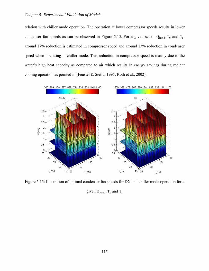
Chapter 5: Experimental Validation of Models
115
relation with chiller mode operation. The operation at lower compressor speeds results in lower
condenser fan speeds as can be observed in Figure 5.15. For a given set of Q , T and T ,
around 17% reduction is estimated in compressor speed and around 13% reduction in condenser
speed when operating in chiller mode. This reduction in compressor speed is mainly due to the
water’s high heat capacity as compared to air which results in energy savings during radiant
cooling operation as pointed in (Feustel & Stetiu, 1995; Roth et al., 2002).
Figure 5.15: Illustration of optimal condenser fan speeds for DX and chiller mode operation for a
given Q , T and T

Chapter 6: Conclusion and Future Work
116
CHAPTER 6
6 Conclusion and Future Work
6.1 Conclusion
In this study models were developed for the components of a vapor compression cycle shown in
Figure 3.1. A semi-empirical approach was taken for modeling of the compression process in a
positive displacement compressor. The heat exchanger models were developed based on
segment-by-segment approach. Flow pattern based correlation were used for modeling heat
transfer and pressure drop in the two-phase region for fan-coil HX while generalized correlations
were used for modeling single-phase heat transfer and pressure drop. In the case of brazed-plate
HX, correlations developed for modeling heat transfer and pressure drop in chevron corrugated
type brazed-plate HX using R-410a as the working fluid were used. The effect of circulating oil
on component parameters was accounted for by using mixture models for calculation of thermo-
physical and transport properties.
A test stand was built from a conventional air conditioning split unit to operate in either chiller
mode or DX mode. A test chamber was also prepared for testing of radiant-cooling with pre-
cooling control as part of the project. Sensors installed on the test stand were calibrated and
instrumentation accuracy was checked by performing energy balance. Speed controls were
implemented on the compressor and condenser fan to assess the savings in low-lift operation of

Chapter 6: Conclusion and Future Work
117
the heat pump. Superheat control was implemented on the expansion valve to maintain any
desired superheat down to 0.5K. Steady state test data was obtained for validation of the
component models and a comparison with the component models presented in (Zakula, 2011,
2010) was performed. Equations for optimal compressor and condenser speeds were developed
to be implemented in operation of test chamber in radiant-cooling operation with pre-cooling
control.
In the compressor model, it was found that for high compressor speeds heat transfer between
suction and discharge becomes important. In the condenser and brazed-plate evaporator, oil was
found to increase the heat transfer due to promotion of annular flow. However, at low refrigerant
flow rates, the heat transfer was found to decrease for fan-coil condenser. The tendency of oil
was to increase pressure drop in HX. A comparison with the component models presented in
(Zakula, 2011, 2010) showed that the current models predict the experimental data with higher
accuracy in case of pressure drop while similar accuracy was estimated for heat transfer. It is to
be noted that the HX models of (Zakula, 2011, 2010) doesn’t take into account effect of oil on
heat transfer and estimates a representative heat transfer coefficient and friction factor for the de-
superheating, sub-cooling, condensation and evaporation regions. However, an inaccurate oil
mass fraction significantly affects the calculation of heat transfer coefficient and friction factor in
the current HX models at high vapor qualities where adverse oil effects are significant. This
results in a higher prediction error as can be seen in the case of fan-coil evaporator. The data set
that was used for fan-coil evaporator comprised of high compressor speeds at which high oil
concentrations are likely to occur as mentioned in (Sarntichartsak et al., 2006). Use of incorrect
oil properties also contribute to higher error estimation. In the case of brazed-plate evaporator,
the current model was found to predict the experimental data with higher accuracy for both heat

Chapter 6: Conclusion and Future Work
118
transfer and pressure drop. Therefore, use of two-phase correlations of (Hsieh & T. F. Lin, 2003)
is recommended for modeling of two-phase heat transfer and pressure drop in brazed-plate HX.
It was also found that solving for air volumetric flow rates for satisfying the HX energy balance
in the system model results in high inaccuracies at low air volumetric flow rates despite small
error in refrigerant mass flow rates. However, as the contribution of condenser fan power and
evaporator fan or pump power in the system power is small, the effect on system performance
prediction is minimal. The system COP is predicted to within ±20% for majority of the data
points. In order to minimize errors in prediction of air volumetric flow rates solution of the
properties for satisfying the HX energy balance that affects the estimation of refrigerant mass
flow rate such as discharge and suction pressure is recommended which is the approach followed
in (Zakula, 2010). From the optimal compressor and condenser fan speed equations, it was found
that during chiller mode both compressor and condenser speeds are lower than DX mode speeds
for delivering the same cooling load for a given outdoor and indoor temperature.
6.2 Future Work
The prediction accuracy of the compressor model over a wide range of pressure ratio and
compressor speeds can be improved by using oil concentration as a function of compressor speed
and incorporation of heat transfer between suction and discharge in the compressor model.
Experimentation needs to be carried out to accurately estimate the oil concentration using any of
the methods mentioned in (Fukuta, Yanagisawa, Miyamura, & Ogi, 2004; Lebreton, Vuillame,
Morvan, & Lottin, 2001; Thome, 2004). Some of these methods are:
1. Measuring oil and refrigerant flow rates leaving an oil separator
2. Withdrawing liquid samples (ASHRAE Standard 41.4-1994)
Chapter 6: Conclusion and Future Work
119
3. Measuring refrigerant-oil mixture density through an accurate density measuring flow
meter
4. Measuring speed of sound of refrigerant-oil liquid mixture through an ultrasonic sensor
5. Measuring refractive index of the refrigerant-oil mixture using a laser displacement
sensor
Oil properties for POE/VG22 also should be obtained from manufacturer or experimentation to
eliminate oil property errors. Formulation of refrigerant properties equations will greatly reduce
time for solution and will enable the current system model to be used for optimization.
On the MI test stand, following things needs to be carried out:
– Compressor operation at higher speeds to better analyze the phenomenon involved at
high pressure ratio operation and data repeatability.
– Implementation of speed control on evaporator
– Testing of pressure transducers on the dead weight tester for assessment of drift and
repeatability
Implementation of radiant-cooling pre-cooling control in the test chamber using the speed
equations presented in this study needs to be carried out to check the validity of the results
and validation of savings estimated for hot and humid climates in (P. R. Armstrong, Jiang,
Winiarski, Katipamula, & Norford, 2009).

Appendix A: Test Stand Components and Instrumentation Description
120
Appendix A
7 Test Stand Components and Instrumentation Description
Table 7.1 and Table 7.2 describe the function of the components installed on the test stand and
test chamber including control devices description and instrumentation details.
Table 7.1: Test stand and test chamber components description
Name Function Specific Details
Mr. Slim compressor
(KNB092FPAH)
Provide lift and refrigerant
flow for cooling
6 pole permanent magnet single rotary
compressor
Rated motor power: 650W
Rotor Locked Amps (RLA): 7.8A
Winding resistance (@20°C): 0.49A
Outdoor fan coil unit
MUZA09NA-1
Air cooled condenser for
rejection of heat to
surroundings
Fin and tube HX with brushless DC fan motor
Brazed-Plate HX
(GB240H-14)
Evaporator for chilled water
circuit
Length:458mm
Width: 86mm
Number of plates: 14
Corrugation type: Chevron
Chevron angle: 65°
Corrugation amplitude: 2mm
Corrugation pitch: 6.8mm
Indoor fan coil unit
MSA09NA Evaporator for DX circuit Fin and tube HX with DC fan motor
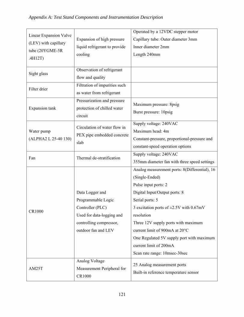
Appendix A: Test Stand Components and Instrumentation Description
121
Linear Expansion Valve
(LEV) with capillary
tube (20YGME-5R
.4H12T)
Expansion of high pressure
liquid refrigerant to provide
cooling
Operated by a 12VDC stepper motor
Capillary tube: Outer diameter 3mm
Inner diameter 2mm
Length 240mm
Sight glass Observation of refrigerant
flow and quality
Filter drier Filtration of impurities such
as water from refrigerant
Expansion tank
Pressurization and pressure
protection of chilled water
circuit
Maximum pressure: 8psig
Burst pressure: 10psig
Water pump
(ALPHA2 L 25-40 130)
Circulation of water flow in
PEX pipe embedded concrete
slab
Supply voltage: 240VAC
Maximum head: 4m
Constant-pressure, proportional-pressure and
constant-speed operation options
Fan Thermal de-stratification Supply voltage: 240VAC
355mm diameter fan with three speed settings
CR1000
Data Logger and
Programmable Logic
Controller (PLC)
Used for data-logging and
controlling compressor,
outdoor fan and LEV
Analog measurement ports: 8(Differential), 16
(Single-Ended)
Pulse input ports: 2
Digital Input/Output ports: 8
Serial ports: 5
3 excitation ports of ±2.5V with 0.67mV
resolution
Three 12V supply ports with maximum
current limit of 900mA at 20°C
One Regulated 5V supply port with maximum
current limit of 200mA
Scan rate range: 10msec-30sec
AM25T
Analog Voltage
Measurement Peripheral for
CR1000
25 Analog measurement ports
Built-in reference temperature sensor

Appendix A: Test Stand Components and Instrumentation Description
122
Used for thermocouple
measurement
SDMAO4
Analog voltage output
peripheral for CR1000
Used for providing speed
signal to outdoor fan
Voltage range: ±5V
Resolution: 2.5mV
Accuracy: 0.5% of Voltage+5mV
SDMIO16
Digital Input/Output
peripheral for CR1000
Used for frequency
measurements and
controlling LEV
Maximum frequency: 2kHz
Accuracy: ±0.01%
Output sink current: 8.6mA for 5V source
Maximum output current: power supply
current limit
SDM16AC
AC/DC relay controller
peripheral for CR1000
Used for control of test
chamber thermal loads and
water pump
Relay type: single pole double throw
Contact rating: 0.3A@ 110VDC, 5A @
30VDC, 110VAC, 277VAC
Coil voltage: 9-18VDC
LEV Controller Stepper motor controller
PIC14F4431 microcontroller for generating
pulses for stepper motor
ULN2003 for switching voltage levels from
5V to 12V for stepper motor operation
Analog input
FR720S-80s VFD Compressor speed controller
For general purpose magnetic flux control
Motor Constant R: 531Ω1
Rated voltage:70V
Rated frequency:120Hz
For linear V/f control V/f ratio: 1.3
Base frequency: 300Hz
Acceleration time: 3sec
Deceleration time:0.1sec
Max frequency: 300Hz
Starting frequency: 5Hz
Current limit: 8A
PWM carrier frequency: 15kHz

Appendix A: Test Stand Components and Instrumentation Description
123
Serial communication
BMC6A01 VFD Outdoor fan speed controller
Maximum speed: 1750rpm
Acceleration time: 1.5sec
Deceleration time: 0.1sec
Current limit: 1.5A
PWM carrier frequency: 2kHz
Analog input
WT1600 Electric power measurement
device
Current range: 5mA-50A
Voltage range: 1.5V-1000V
Voltage Accuracy: 0.3% of reading + 0.1% of
range
Current accuracy: (0.015*frequency in
kHz+0.3)% of reading +0.2% of range
Power accuracy: (0.02*frequency in
kHz+0.3)% of reading +0.2% of range
Analog output
1. The values indicate the parameters value programmed into the VFD
Table 7.2: Test stand and test chamber sensors description
Name Function Specific Details1
Honeywell MLH-500
Gauge pressure transducer for
refrigerant pressure
measurement
Accuracy: ±5% full scale @>300psig
±10% full scale @100-299psig
Supply voltage: 5 ± 0.25VDC
Analog output: 0.5-4.5VDC
Measurement
Specialties SSI-500
Gauge pressure transducer for
refrigerant pressure
measurement
Accuracy: ±1% full scale
Supply voltage: 5VDC
Analog output: 0-100mVDC
Measurement
Specialties US300
Absolute pressure transducer
for ambient pressure
measurement
Accuracy: ±0.15% full scale
Supply voltage: 5VDC
Current output: 4-20mA

Appendix A: Test Stand Components and Instrumentation Description
124
Type T Thermocouple Temperature measurement Accuracy:±0.1°C
Analog output
Micromotion ELITE
series
Refrigerant mass flow rate
measurement
Supply voltage: 240VAC
Accuracy: ±0.05% of reading
Repeatability: ±0.025% of reading
Frequency output
Hansen Technologies
SHP-06
Brazed-Plate HX refrigerant
level measurement
Linearity :±0.5% of reading
Supply voltage: 11-36VDC
Maximum pressure: 400psig
Analog output: 0-5VDC
GEMU 3030 magnetic
water flow meter
Chilled water flow rate
measurement
Supply voltage: 24VDC
Accuracy: ±1% full scale
Pulse output
Watt Node
WNB-3Y-400-P Electric power measurement
Accuracy: ±0.5% of reading
Pulse output
LICOR Pyranometer Solar radiation measurement Accuracy: ±5% of reading
Current output
Honeywell HIH4000
Humidity sensor
Test chamber humidity
measurement
Accuracy: ±3.5%
Repeatability: ±0.5%
Hysteresis: 3%
Analog output
1. Datasheet values are reported

Appendix B: Data Logging and Controlling Code for Test Stand Instruments
125
Appendix B
8 Data Logging and Controlling Code for Test Stand Instruments
'CR1000 Series Datalogger 'Logging code for Abu Dhabi low lift chiller system 'program author: Muhammad Tauha Ali & Nicholas Gayeski 'date: May 2011 'Declare Reference Variables Public CR1000Temp, AM25Temp, AM25Temp0, batt_volt, sdmstat, serialstat, es, Public comp_voltage,comp_current, comp_current_limit=5.7, failmode, suction_timer=0, timer_flag=0,suction_timer_set=60, zone_timer=0, zone_flag=0,zone_timer_set=5, delay_timer=200, delay_flag=0, delay_timer_set=120'failsafe Public Qe,Tz,f,rpm,TxK,TzK 'model based speed control Public log_result, water_flow, pump_power, slab_temp(20), room_temp(19), Ptemp, Iload '+++++ Public rpm_sensor Public GHI_South, GHI_West, Tsouth, Twest Public PambairkPa, RelativeHumidity, room_temp_NW, Tdew, Tglobe, SpecificHumidity, Tdew1 Public PdisPSIG, PcondoutPSIG, PevapinPSIG, PsucPSIG Public RTdischarge, RTcondin, RTcondout, RTdrierin, RTdrierout 'high side temp Public RTpostLEV, RTsuction, RTsuction1 'low side temp Public RTHXin, RTHXout, CHWTin, CHWTout 'HX inlet and outlet 'Public RTcondout1,RTcondoutlevhigh1small,RTcondoutlevhigh2big,RTcondoutlevlow1small,RTcondoutlevlow2big 'tcondout error check Public ATcondenserin, ATdelTcondenser, delta_mV, Tref, dTresult, mV_TdT 'condenser thermopile Public fan_totpower,fan_angle,fan_power,VFDpowerin,comp_totpower,comp_angle,comp_power Public ref_mass_flow Public Psat, Tsat 'for saturation temperature Public Tsatcond, Tsubcool, Tsubcool_set=5 'subcool control Public Tsatsuc,Tsuperheat,Tsuperheat_set=2,Tsatdis,Tsuperheatdis 'superheat control Public refrigerant_level,refrigerant_level_set=95 'refrigerant level control Public frequency_set_old As Long,frequency_set As Long,VFD_control_old As Long,VFD_control As Long, VFD_relay_old 'VFD control Public fan_speed_set, fan_speed_max=1000,volt_signal(4) 'fan speed control Public LEV_Kp,LEV_Ki,LEV_Kd,errvarLEV_old,errvarLEV=0,intgrlLEV=0,LEVcorr_0,LEVcorr,LEV_Kpold, LEV_Kiold, LEV_Kdold,LEVpos=0,del As Long,LEV_operation(16) 'LEVcontrol Public speed_Kp,speed_Ki,speed_Kd,errvarspeed_old,errvarspeed=0,intgrlspeed=0,speedcorr_0,speedcorr,speed_Kpold, speed_Kiold, speed_Kdold 'speed control Public cntrlvarLEV,cntrlvarLEV_set,cntrlvarLEV_set_old,cntrlvarspeed,cntrlvarspeed_set,cntrlvarspeed_set_old,Tz_set=24, dead_band_speed=.5 'control variables Alias RTdrierout=RTpreLEV Alias ATcondenserin=Tx Alias LEV_operation(1)=LEV_open Alias LEV_operation(2)=LEV_close
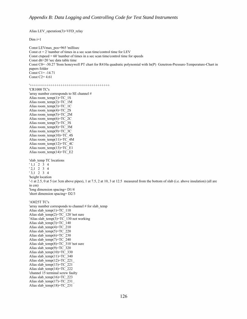
Appendix B: Data Logging and Controlling Code for Test Stand Instruments
126
Alias LEV_operation(3)=VFD_relay Dim i=1 Const LEVmax_pos=965 'millisec Const ct = 2 'number of times in a sec scan time/control time for LEV Const ctspeed = 60 'number of times in a sec scan time/control time for speeds Const dtt=20 'sec data table time Const C0= -30.27 'from honeywell PT chart for R410a quadratic polynomial with ln(P) Genetron-Pressure-Temperature-Chart in papers folder Const C1= -14.71 Const C2= 4.61 '+++++++++++++++++++++++++++++++++++++++ 'CR1000 TC's 'array number corresponds to SE channel # Alias room_temp(1)=TC_1S Alias room_temp(2)=TC_1M Alias room_temp(3)=TC_1C Alias room_temp(4)=TC_2S Alias room_temp(5)=TC_2M Alias room_temp(6)=TC_2C Alias room_temp(7)=TC_3S Alias room_temp(8)=TC_3M Alias room_temp(9)=TC_3C Alias room_temp(10)=TC_4S Alias room_temp(11)=TC_4M Alias room_temp(12)=TC_4C Alias room_temp(13)=TC_E1 Alias room_temp(14)=TC_E2 'slab_temp TC locations ' 1,1 2 3 4 ' 2,1 2 3 4 ' 3,1 2 3 4 'height location '-1 at 2.5, 0 at 5 (or 3cm above pipes), 1 at 7.5, 2 at 10, 3 at 12.5 measured from the bottom of slab (i.e. above insulation) (all are in cm) 'long dimension spacing= D1/4 'short dimension spacing= D2/3 'AM25T TC's 'array number corresponds to channel # for slab_temp Alias slab_temp(1)=TC_110 Alias slab_temp(2)=TC_120 'not sure 'Alias slab_temp(3)=TC_130 not working Alias slab_temp(3)=TC_140 Alias slab_temp(4)=TC_210 Alias slab_temp(5)=TC_220 Alias slab_temp(6)=TC_230 Alias slab_temp(7)=TC_240 Alias slab_temp(8)=TC_310 'not sure Alias slab_temp(9)=TC_320 Alias slab_temp(10)=TC_330 Alias slab_temp(11)=TC_340 Alias slab_temp(12)=TC_221_ Alias slab_temp(13)=TC_221 Alias slab_temp(14)=TC_222 'channel 15 terminal screw faulty Alias slab_temp(16)=TC_223 Alias slab_temp(17)=TC_231_ Alias slab_temp(18)=TC_231

Appendix B: Data Logging and Controlling Code for Test Stand Instruments
127
Alias slab_temp(19)=TC_232 Alias slab_temp(20)=TC_233 Alias room_temp(15)=TC_W2 'channel 21 Alias room_temp(16)=TC_W1 'channel 22 Alias room_temp(17)=TC_SW 'channel 23 Alias room_temp(18)=TC_SE 'channel 24 Alias room_temp(19)=TC_NE 'channel 25 Alias water_flow=flow_rate_l_sec Alias pump_power=power_W 'Define Data Tables DataTable (room_temp,1,-1) DataInterval (0,2,Min,10) Average(1,TC_1S,IEEE4,false) Average(1,TC_1M,IEEE4,false) Average(1,TC_1C,IEEE4,false) Average(1,TC_2S,IEEE4,false) Average(1,TC_2M,IEEE4,false) Average(1,TC_2C,IEEE4,false) Average(1,TC_3S,IEEE4,false) Average(1,TC_3M,IEEE4,false) Average(1,TC_3C,IEEE4,false) Average(1,TC_4S,IEEE4,false) Average(1,TC_4M,IEEE4,false) Average(1,TC_4C,IEEE4,false) Average(1,TC_E1,IEEE4,false) Average(1,TC_E2,IEEE4,false) Average(1,TC_NE,IEEE4,false) Average(1,TC_W2,IEEE4,false) Average(1,TC_W1,IEEE4,false) Average(1,TC_SW,IEEE4,false) Average(1,TC_SE,IEEE4,false) EndTable DataTable (slab_temp,1,-1) DataInterval (0,2,Min,10) Average(1,PTemp,IEEE4,false) Average(1,TC_110,IEEE4,false) Average(1,TC_120,IEEE4,false) 'not sure 'Average(1,TC_130,IEEE4,false)'not working Average(1,TC_140,IEEE4,false) Average(1,TC_210,IEEE4,false) Average(1,TC_220,IEEE4,false) Average(1,TC_230,IEEE4,false) Average(1,TC_240,IEEE4,false) Average(1,TC_310,IEEE4,false)'not sure Average(1,TC_320,IEEE4,false) Average(1,TC_330,IEEE4,false) Average(1,TC_340,IEEE4,false) Average(1,TC_221_,IEEE4,false) Average(1,TC_221,IEEE4,false) Average(1,TC_222,IEEE4,false) Average(1,TC_223,IEEE4,false) Average(1,TC_231_,IEEE4,false) Average(1,TC_231,IEEE4,false) Average(1,TC_232,IEEE4,false) Average(1,TC_233,IEEE4,false) EndTable DataTable (pump_performance,1,-1) DataInterval (0,2,Min,10)

Appendix B: Data Logging and Controlling Code for Test Stand Instruments
128
Average (1,flow_rate_l_sec,IEEE4,false) StdDev (1,flow_rate_l_sec,IEEE4,False) Average (1,power_W,IEEE4,false) StdDev (1,power_W,IEEE4,false) EndTable '+++++++++++++++++++++++++++++++++++++ 'Define Data Tables DataTable (test_stand1,1,-1) DataInterval (0,2,Min,10) Minimum (1,batt_volt,IEEE4,0,False) 'Average (1,CR1000Temp,IEEE4,) Average (1,AM25Temp,IEEE4,False) Average (1,fan_speed_set,IEEE4,False) Average (1,frequency_set_old,IEEE4,False) Average (1,PambairkPa,IEEE4,False) Average (1,RelativeHumidity,IEEE4,False) Average (1,Tz,IEEE4,False) Average (1,room_temp_NW,IEEE4,False) Average (1,Tdew,IEEE4,False) Average (1,SpecificHumidity,IEEE4,False) ' Average (1,Tglobe,IEEE4,False) Average (1,Tx,IEEE4,False) Average (1,ATdelTcondenser,IEEE4,False) Average (1,RTcondin,IEEE4,False) Average (1,RTpreLEV,IEEE4,False) Average (1,RTpostLEV,IEEE4,False) ' Average (1,VFDpowerin,IEEE4,False) Average (1,comp_power,IEEE4,False) Average (1,fan_Power,IEEE4,False) Average (1,GHI_South,IEEE4,False) Average (1,GHI_West,IEEE4,False) Average (1,Tsouth,IEEE4,False) Average (1,Twest,IEEE4,False) ' Average (1,refrigerant_level,FP2,False) Average (1,comp_voltage,IEEE4,False) Average (1,comp_angle,IEEE4,False) EndTable DataTable (test_stand0,1,-1) DataInterval (0,2,Min,10) Average (1,PdisPSIG,IEEE4,False) Average (1,PcondoutPSIG,IEEE4,False) Average (1,PevapinPSIG,IEEE4,False) Average (1,PsucPSIG,IEEE4,False) Average (1,RTdischarge,IEEE4,False) Average (1,RTcondout,IEEE4,False) Average (1,RTsuction,IEEE4,False) Average (1,RTHXin,IEEE4,False) Average (1,RTHXout,IEEE4,False) Average (1,CHWTin,IEEE4,False) Average (1,CHWTout,IEEE4,False) Average (1,Tsuperheat,IEEE4,False) Average (1,Tsuperheatdis,IEEE4,False) Average (1,Tsubcool,IEEE4,False) Average (1,comp_current,IEEE4,False) Average (1,ref_mass_flow,IEEE4,False) Average (1,rpm_sensor,IEEE4,False) EndTable Sub actLEV(cntrlvarLEV) Call LEVcontrol(cntrlvarLEV)

Appendix B: Data Logging and Controlling Code for Test Stand Instruments
129
If i<>0 'for zero excitation when valve is fully closed or open If LEVcorr>0'cntrlvar<cntrlvar_set 'open valve red light C2 del=ABS(LEVcorr) 'If del>LEVmax_pos*1000 Then 'for crash prevention (from NANs) not working 'Else If del>3 '3msec is the delay of microcontroller 'WriteIO(&B00100000,&B00100000) 'C6 LEV_open=1 SDMIO16(LEV_operation,sdmstat,0,94,0,0,0,0,1,0) Delay (1,del,mSec)'LEVcorr is the amount of time excitation remains there LEV_open=0 SDMIO16(LEV_operation,sdmstat,0,94,0,0,0,0,1,0) 'WriteIO(&B00100000,&B00000000) LEVpos=LEVpos+LEVcorr EndIf 'EndIf ElseIf LEVcorr<0'cntrlvar>cntrlvar_set 'close valve green light C3 del=ABS(LEVcorr) 'If del>LEVmax_pos*1000 Then 'Else If del>3 'WriteIO(&B01000000,&B01000000) 'C7 LEV_close=1 SDMIO16(LEV_operation,sdmstat,0,94,0,0,0,0,1,0) Delay (1,del,mSec)'LEVcorr is the amount of time excitation remains there LEV_close=0 SDMIO16(LEV_operation,sdmstat,0,94,0,0,0,0,1,0) 'WriteIO(&B01000000,&B00000000) LEVpos=LEVpos+LEVcorr EndIf 'EndIf EndIf If LEVpos>LEVmax_pos LEVpos=LEVmax_pos ElseIf LEVpos<0 LEVpos=0 'can't be less than 0 EndIf EndIf EndSub Sub LEVcontrol(cntrlvarLEV) errvarLEV=cntrlvarLEV_set-cntrlvarLEV If (ABS(cntrlvarLEV_set-cntrlvarLEV_set_old)+ABS(LEV_Kp-LEV_Kpold)+ABS(LEV_Ki-LEV_Kiold)+ABS(LEV_Kd-LEV_Kdold))>0 OR LEVpos>LEVmax_pos OR LEVpos<=0 Then intgrlLEV=0 'Resset Intergal term if the setpoint or gains are changed or valve is at saturation EndIf LEVcorr_0=LEV_Kp*errvarLEV+LEV_Kp*(intgrlLEV+1/ct*errvarLEV)/LEV_Ki+LEV_Kp*LEV_Kd*(errvarLEV-errvarLEV_old)*ct 'control line LEVcorr=Round(LEVcorr_0,0) If (cntrlvarLEV_set<cntrlvarLEV AND LEVcorr>0) Then 'correct for incorrect valve operation and wrong correction (have encountered) LEVcorr=-LEVcorr ElseIf (cntrlvarLEV_set>cntrlvarLEV AND LEVcorr<0) Then LEVcorr=LEVcorr EndIf 'If (LEVcorr-LEV_pos) > LEVmax_del Then 'limit for positive extreme of pulses (correction that CR1000 can handle w/o skipping scans) depends on scan time (not needed for 1 sec) ' LEVcorr=LEVmax_pos+LEV_pos 'ElseIf (LEVcorr-LEV_pos) < -LEVmax_del Then 'limit for negative extreme of pulses
Appendix B: Data Logging and Controlling Code for Test Stand Instruments
130
' LEVcorr =-LEVmax_pos+LEV_pos 'EndIf 'integral routine If LEVcorr>LEVmax_pos Then 'for max time limit/valve position LEVcorr=LEVmax_pos If errvarLEV > 0 Then intgrlLEV=intgrlLEV+errvarLEV*1/ct 's(k-1) integral summing EndIf ElseIf LEVcorr<-LEVmax_pos Then 'for max time limit/valve position LEVcorr =-LEVmax_pos If errvarLEV < 0 Then intgrlLEV=intgrlLEV+errvarLEV*1/ct 's(k-1) integral summing EndIf Else intgrlLEV=intgrlLEV+errvarLEV*1/ct 's(k-1) integral summing EndIf 'LEVcorr_a=LEVcorr-LEV_pos 'refrigrant_level_set_old=refrigerant_level_set errvarLEV_old=errvarLEV cntrlvarLEV_set_old=cntrlvarLEV_set LEV_Kpold=LEV_Kp LEV_Kiold=LEV_Ki LEV_Kdold=LEV_Kd If (LEVpos>=LEVmax_pos AND LEVcorr>0) Then ' not to operate valve if already fully open or closed LEVcorr=0 intgrlLEV=0 i=0 ElseIf (LEVpos<=0 AND LEVcorr<0) Then LEVcorr=0 intgrlLEV=0 i=0 EndIf EndSub Sub Failsafe If CHWTin<5 OR CHWTout<5 OR Tz<10 OR RTdischarge>85 OR Tsatdis>60 OR comp_current>=7 OR comp_current=Nan frequency_set=0 VFD_control=0 ModBusMaster(serialstat,Com3,19200,1,16,VFD_control,9,1,3,10) 'change VFD operation status start (2)/stop(0 or 1) ModBusMaster(serialstat,Com3,19200,1,16,frequency_set,14,1,3,10) 'change running VFD frequency ModBusMaster(serialstat,Com3,19200,1,3,frequency_set_old,14,1,3,10) 'read running VFD frequency failmode=1 delay_timer=Timer(3,Sec,2) 'reset and start delay_timer delay_flag=1 EndIf If RTsuction1<-2 AND timer_flag=0 suction_timer=Timer(1,Sec,2) 'reset and start suction_timer timer_flag=1 EndIf suction_timer=Timer(1,Sec,4) If RTsuction1<-2 AND suction_timer>suction_timer_set 'if Tsuction remains at -2 for 1 minute frequency_set=0 VFD_control=0 ModBusMaster(serialstat,Com3,19200,1,16,VFD_control,9,1,3,10) 'change VFD operation status start (2)/stop(0 or 1) ModBusMaster(serialstat,Com3,19200,1,16,frequency_set,14,1,3,10) 'change running VFD frequency ModBusMaster(serialstat,Com3,19200,1,3,frequency_set_old,14,1,3,10) 'read running VFD frequency failmode=2 delay_timer=Timer(3,Sec,2) 'reset and start delay_timer suction_timer=Timer(1,Sec,3) 'stop and reset suction_timer timer_flag=0 ElseIf suction_timer>suction_timer_set
Appendix B: Data Logging and Controlling Code for Test Stand Instruments
131
suction_timer=Timer(1,Sec,3) 'reset and stop suction_timer timer_flag=0 EndIf EndSub 'Main Program BeginProg 'for LEV control with Tsuperheat LEV_Kp=5 LEV_Kpold=LEV_Kp LEV_Ki= 45 LEV_Kiold=LEV_Ki LEV_Kd= 11.25 LEV_Kdold=LEV_Kd 'for speed control with Tz speed_Kp=5000 speed_Kpold=speed_Kp speed_Ki= 100000 speed_Kiold=speed_Ki speed_Kd= 0 speed_Kdold=speed_Kd 'initialization frequency_set=10000 frequency_set_old=frequency_set fan_speed_set=1000 VFD_control=0 VFD_control_old=VFD_control VFD_relay=0 VFD_relay_old=VFD_relay cntrlvarLEV_set_old=cntrlvarLEV_set cntrlvarspeed_set_old=cntrlvarspeed_set f=63 rpm=0 SDMIO16(LEV_operation,sdmstat,0,89,0,0,0,0,0111,0) 'don't know why it doesn't work sometimes with 94 if restart cr1000 'initialization for controls ModBusMaster(serialstat,Com3,19200,1,16,VFD_control,2,1,3,10) 'for resetting VFD .1msec delay 'SW12(1) '12V power for control circuit 'WriteIO(&B10000000,&B00000000) 'relay on (currently off) 'WriteIO(&B00100000,&B00100000) 'to bring the valve to its fully close position green light C4 LEV_close=1 SDMIO16(LEV_operation,sdmstat,0,94,0,0,0,0,1,0) Delay (1,3,Sec)'LEVcorr is the amount of time excitation remains there LEV_close=0 SDMIO16(LEV_operation,sdmstat,0,94,0,0,0,0,1,0) 'WriteIO(&B00100000,&B00000000) 'SDMIO16(LEV_close,sdmstat,0,89,9999,9999,9999,9990,1,0) ModBusMaster(serialstat,Com3,19200,1,3,VFD_control_old,9,1,3,10) 'read VFD operation status ModBusMaster(serialstat,Com3,19200,1,16,frequency_set,14,1,3,10) 'set VFD frequency = 0Hz volt_signal(1)=0 '1rpm=2.857mV SDMAO4(volt_signal(1),1,1) Scan (ct,Sec,0,0) AM25T (AM25Temp0,0,mV2_5,1,1,TypeT,AM25Temp0,4,8,Vx1,True ,0,_50Hz,1.0,0)
Appendix B: Data Logging and Controlling Code for Test Stand Instruments
132
' Refrigerant pressures VoltDiff (PdisPSIG,1,mV250C,5,True ,0,_50Hz,4.977,1.55) 'calibrated transducer number 3 VoltSe (PcondoutPSIG,1,mv5000,13,True,0,_50Hz,123.9e-3,-63.1) 'calibrated transducer number 5 VoltSe (PevapinPSIG,1,mv5000,14,True,0,_50Hz,124.7e-3,-63.83) 'calibrated transducer number 8 VoltDiff (PsucPSIG,1,mV250C,6,True ,0,_50Hz,4.945,-6.467) 'calibrated transducer number 1 ' Refrigerant temperatures 'high side temperatures AM25T (RTdischarge,1,mV2_5,1,1,TypeT,AM25Temp0,4,8,Vx1,True ,0,_50Hz,1.0,0) ' soldered AM25T (RTcondout,1,mV2_5,3,1,TypeT,AM25Temp0,4,8,Vx1,True ,0,_50Hz,1.0,0) ' soldered AM25T (RTsuction,1,mV2_5,8,1,TypeT,AM25Temp0,4,8,Vx1,True ,0,_50Hz,1.0,0) ' soldered AM25T (RTHXin,1,mV2_5,7,1,TypeT,AM25Temp0,4,8,Vx1,True ,0,_50Hz,1.0,0) ' soldered AM25T (RTHXout,1,mV2_5,12,1,TypeT,AM25Temp0,4,8,Vx1,True ,0,_50Hz,1.0,0) ' soldered 'chilled water temperatures AM25T (CHWTin,1,mV2_5,9,1,TypeT,AM25Temp0,4,8,Vx1,True ,0,_50Hz,1.0,0) ' soldered AM25T (CHWTout,1,mV2_5,10,1,TypeT,AM25Temp0,4,8,Vx1,True ,0,_50Hz,1.0,0) ' soldered 'to calculate superheat Tsatsuc=C2*(LN(PsucPSIG+14.5))^2+C1*(LN(PsucPSIG+14.5))+C0 Tsuperheat=RTsuction-Tsatsuc Tsatdis=C2*(LN(PdisPSIG+14.5))^2+C1*(LN(PdisPSIG+14.5))+C0 Tsuperheatdis=RTdischarge-Tsatdis 'to calculate subcooling Tsatcond=C2*(LN(PcondoutPSIG+14.7))^2+C1*(LN(PcondoutPSIG+14.7))+C0 Tsubcool=Tsatcond-RTcondout i=1 cntrlvarLEV=-Tsuperheat 'can make any variable control varaiable as long as error (set-actual) follows for > valve open for < valve close 'parameter s>a s<a actual increase actual decrease 'ref. level open close open close 'Tsubcool open close open close 'Tsuperheat close open close open (if multiply by -1 both set and actual then s>a open s<a close) 'Tsuperheatcond close open close open (if multiply by -1 both set and actual then s>a open s<a close) 'Q decrease increase speed decrease speed increase cntrlvarLEV_set=-Tsuperheat_set Call actLEV(cntrlvarLEV) ' mass flow rate PulseCount (ref_mass_flow,1,2,0,1,3e-6,0) 'Refrigerant '10000Hz=.03 kg/sec so for 1 Hz 3e-6 ' rpm sensor PulseCount(rpm_sensor,1,1,2,1,60,0) 'to prevent compressor stall and decrease compressor current AM25T(comp_current,1,mv5000,18,1,-1,AM25Temp0,4,8,Vx1,False,0,_50Hz,.002,0) Call Failsafe CallTable test_stand0 PulseCountReset NextScan SlowSequence Scan(dtt,Sec,0,0)
Appendix B: Data Logging and Controlling Code for Test Stand Instruments
133
If VFD_relay<>VFD_relay_old SDMIO16(LEV_operation,sdmstat,0,94,0,0,0,0,1,0) VFD_relay_old=VFD_relay EndIf If frequency_set<>frequency_set_old ModBusMaster(serialstat,Com3,19200,1,16,frequency_set,14,1,3,10) 'change running VFD frequency ModBusMaster(serialstat,Com3,19200,1,3,frequency_set_old,14,1,3,10) 'read running VFD frequency EndIf volt_signal(1)=fan_speed_set*(2.857+.0857)+1.9 '1rpm=2.857mV SDMAO4(volt_signal(1),1,1) If VFD_control<>VFD_control_old ModBusMaster(serialstat,Com3,19200,1,16,VFD_control,9,1,3,10) 'change VFD operation status start (2)/stop(0 or 1) VFD_control_old=VFD_control EndIf 'Panel Temperatures and references AM25T (AM25Temp,0,mV2_5,1,1,TypeT,AM25Temp,4,8,Vx1,True ,0,_50Hz,1.0,0) 'PanelTemp (CR1000Temp,_50Hz) Battery (Batt_volt) ' Air pressure VoltDiff (PambairkPa,1,mv5000,8,True,0,_50Hz,3.939e-3,-3.75) '238 ohm, 4-20 mA output, 4760 mV = 15 psia, 952 mV = 0 psia PambairkPa=PambairkPa*6.89476 'zone relative humidity VoltSe (RelativeHumidity, 1,mv5000,3,True,0,_50Hz,0.032258,-25.80645) 'zone temperature AM25T (room_temp_NW,1,mV2_5,13,1,TypeT,AM25Temp,4,8,Vx1,True ,0,_50Hz,1.0,0) ' AM25T (Tglobe,1,mV2_5,14,1,TypeT,AM25Temp,4,6,Vx1,True ,0,_50Hz,1.0,0) es=6.1121*EXP((18.678-room_temp_NW/234.5)*room_temp_NW/(257.14+room_temp_NW)) 'arden buck equation 1996 'Tdew1=(237.7*LOG10(es*RelativeHumidity/611))/(7.5-LOG10(es*RelativeHumidity/611)) SpecificHumidity=.62197*(es*RelativeHumidity/100)/(PambairkPa*10+(es*RelativeHumidity/100)*(.62197-1)) DewPoint(Tdew,room_temp_NW,RelativeHumidity) If Tdew>room_temp_NW OR Tdew=NAN Then Tdew=room_temp_NW ' Air Temperature AM25T (ATcondenserin,1,mV2_5,11,1,TypeT,AM25Temp,4,8,Vx1,True ,0,_50Hz,1.0,0) ' Scaling for thermopile measurement AM25T (delta_mV,1,mV25C,16,1,-1,AM25Temp,4,8,Vx1,True ,0,_50Hz,1.0,0) delta_mV = delta_mV/16 '16 thermopile junction pairs Tref = ATcondenserin 'delta_mV = delta_mV*0.1 'to avoid exponents in equation of volt to temp conversion dTresult 'TdTref = TdTref*0.01 'mV_TdT = delta_mV*TdTref*0.001' for bringing it in Volts dTresult = 25.89-5.749e-2*Tref-.7447*delta_mV+1.632e-4*Tref^2+5.557e-3*Tref*delta_mV+.4654*delta_mV^2-.4475e-6*Tref^3-2.107e-5*Tref^2*delta_mV-3.793e-4*Tref*delta_mV^2-2.188e-3*delta_mV^3 'volt to temp conversion 'dTresult = dTresult-5.749*TdTref+1.635*TdTref-0.4475*TdTref 'dTresult = dTresult+mV_TdT*5.557-2.107*mV_TdT*TdTref-3.793*mV_TdT*delta_mV 'delta_mV = delta_mV*10 ATdelTcondenser = dTresult*delta_mV 'TdTref = TdTref*100 ' end of scaling for thermopile measurement ' Wattnode power

Appendix B: Data Logging and Controlling Code for Test Stand Instruments
134
'PulseCount (VFDpowerin,1,1,0,1,34.506,0) ' WNB-3Y-400-P, Wh per pulse per CT rated Amp = 0.001917 ' 59.7 ohm resistor installed = 5 Amps full scale ' WhpP = 0.0096 ' Watts = WhpP*PulseCount/sec*3600 sec/hour ' W/Hz = WhpP*3600 sec/hour = 34.506 Watts AM25T (RTcondin,1,mV2_5,2,1,TypeT,AM25Temp,4,8,Vx1,True ,0,_50Hz,1.0,0) ' soldered 'low side temperatures AM25T (RTpostLEV,1,mV2_5,6,1,TypeT,AM25Temp,4,8,Vx1,True ,0,_50Hz,1.0,0) ' soldered 'to see drier temperature drop which implies pressure drop 'AM25T (RTdrierin,1,mV2_5,4,1,TypeT,AM25Temp,4,8,Vx1,True ,0,_50Hz,1.0,0) ' soldered AM25T (RTdrierout,1,mV2_5,5,1,TypeT,AM25Temp,4,8,Vx1,True ,0,_50Hz,1.0,0) ' soldered VoltSe(GHI_South,1,mV25,4,True,0,_50Hz,-86.704,0) 'PY64287 1/(78.7e-3*146.55ohm) VoltSe(GHI_West,1,mV25,5,True,0,_50Hz,-85.03,0) 'PY64288 1/(78.93e-3*149ohm) AM25T (Tsouth,1,mV2_5,25,1,TypeT,AM25Temp,4,8,Vx1,True ,0,_50Hz,1.0,0) 'epoxied AM25T (Twest,1,mV2_5,24,1,TypeT,AM25Temp,4,8,Vx1,True ,0,_50Hz,1.0,0) ' epoxied ' Measure refrigerant level VoltSe (refrigerant_level,1,mv5000,6,True,0,_50Hz,16.67e-3,16.67) '3321.15mV=100 level 1mV=.03006153596 level (not applicable) GetVariables(log_result,ComRS232,0,2,0,0,"Public","room_temp()",room_temp(),19) Tz=(room_temp(1)+room_temp(2)+room_temp(3)+room_temp(4)+room_temp(5)+room_temp(6)+room_temp(7)+room_temp(8)+room_temp(9)+room_temp(10)+room_temp(11)+room_temp(12)+room_temp(13)+room_temp(14)+room_temp(15)+room_temp(16)+room_temp(17)+room_temp(18)+room_temp(19)+room_temp_NW)/20 ''''cntrlvarspeed=-Tz ''''cntrlvarspeed_set=-Tz_set AM25T(comp_voltage,1,mv5000,17,1,-1,AM25Temp,4,8,Vx1,False,0,_50Hz,.06,0) AM25T(comp_angle,1,mv5000,19,1,-1,AM25Temp,4,8,Vx1,False,0,_50Hz,.072,0) AM25T(comp_power,1,mv5000,20,1,-1,AM25Temp,4,8,Vx1,False,0,_50Hz,1.22,0) AM25T(fan_power,1,mv5000,22,1,-1,AM25Temp,4,8,Vx1,False,0,_50Hz,.06,0) CallTable test_stand1 NextScan EndSequence SlowSequence Scan(2,Min,0,0) PakBusClock(2) GetDataRecord(log_result,ComRS232,0,2,0,0,2,&H8001,room_temp) GetDataRecord(log_result,ComRS232,0,2,0,0,2,&H8002,slab_temp) GetDataRecord(log_result,ComRS232,0,2,0,0,2,&H8003,pump_performance) GetRecord(room_temp(),room_temp,1) GetVariables(log_result,ComRS232,0,2,0,0,"Public","Iload",Iload,1) NextScan EndSequence EndProg

Appendix C: Test Chamber Heat Transfer Reduction after Insulation
135
Appendix C
9 Test Chamber Heat Transfer Reduction after Insulation
Data:
Wall is made up of two steel sheets with fiberglass insulation in between
Thickness of wall (t) = 6cm
Insulation thickness = 10cm
k for fiberglass = 0.04W/mK (“Thermal Conductivity of some common Materials,” 2011)
k for polystyrene = 0.0343 W/mK [manufacturer datasheet]
Assumptions:
– Thermal Resistance of steel sheets is negligible.
– Convection and radiation heat transfer is neglected.
– Assume a temperature difference of 10K between the internal walls.
Solution:
QA k
∆Tt
Before insulation: Q = 6.67 W/m2
After insulation: Q = 2.26 W/m2
Percentage reduction: 66%

Appendix D: Air Leakage Testing of Test Chamber
136
Appendix D 10 Air Leakage Testing of Test Chamber
10.1 Air Leakage before Caulking:

Appendix D: Air Leakage Testing of Test Chamber
137
10.2 Air Leakage after Caulking:

Appendix E: Test Chamber Components and Thermocouple Location Description
138
Appendix E 11 Test Chamber Components and Thermocouple Location Description

Appendix F: Gauge Pressure Sensor/ Transducer Calibration Procedure
139
Appendix F
12 Gauge Pressure Sensor/ Transducer Calibration Procedure
1. Close the valve on the nitrogen cylinder pressure regulator.
2. Open the vent valve labeled “<- –“ on the Mensor CPB5000.
3. Remove the plug from the pressure sensor/transducer mounting place on the right side of
CPB5000.
4. Attach the pressure sensor/transducer directly on the mounting or on the ¼” header with
three ports available.
5. Close the vent valve and open the valve labeled “<- +” on CPB5000.
6. Open the valve on the pressure regulator to a suitable pressure value.3*
7. Check the connection for leaks using soap bubble.
8. Clean the soap from the connections after leak testing.
9. Close the valve labeled “<- +” and open the vent valve.
10. Remove the plug from piston mounting place by rotating the ConTect quick connector
anti-clockwise on the left side of the CPB5000.4
11. Place the piston on the mounting and close the ConTect quick connector by rotating in
clockwise direction.
12. Note the ambient temperature and pressure to 0.01% Full Scale (FS) of test article.
3 Do not exceed the maximum limit of the pressure sensor/transducer or CPB5000 which is 100bar/1500psi 4 Use Latex gloves while handling the piston or weights to protect them from dust or scratches. Use Alcohol and a soft cloth for cleaning of the weights

Appendix F: Gauge Pressure Sensor/ Transducer Calibration Procedure
140
13. Use a voltage source stable to four significant digits or CR1000 (for +5V) for excitation
of pressure transducers.
14. Place the weights on the piston to exert the desired pressure on the pressure
sensor/transducer.
15. Open the valve labeled “<- +” and observe the pressure reading on the pressure gauge on
CPB5000.
16. Use the three spoke handle for small increments or decrements in pressure and try to
achieve a stable floating position for the piston.
17. Observe the marking line on the mirror near the piston mounting place as shown in the
figure.

Appendix F: Gauge Pressure Sensor/ Transducer Calibration Procedure
141
18. To minimize the effect of friction, move the system up against the weight pieces carefully
and make a turning movement.5
19. Wait 10-15 seconds to see if the system maintains its position.
20. Observe the reading in the pressure sensor/transducer.
21. Use CR1000 (if possible) for reading voltage from the pressure transducer.
22. Take 6 readings at approximately 0%, 20%, 40%, 60%, 80% and 100% of full scale in
increasing and decreasing manner each.
23. Plot the regression line to get the multiplier and offset for the pressure sensor/transducer.
Report standard errors and t-statistics.
24. After finishing calibration, close the valve on the pressure regulator and release the
pressure by opening the vent valve on CPB5000.
25. Remove the piston and pressure transducers from CPB5000 and put back the plugs.
26. Cover CPB5000 to protect it from dust.
5 Never move the system up and make a turning movement, if the piston is in the lower or upper block position.

Appendix G: Test Stand Data for DX Mode of Operation
142
Appendix G
13 Test Stand Data for DX Mode of Operation
Refrigerant Temperatures Refrigerant Pressures
Comp-ressor Speed (Hz)
Zone Air Temp (°C)
Outdoor Air Temp
(°C)
Discharge Temp (°C)
Condenser Inlet Temp
(°C)
Condenser Outlet Temp
(°C)
Suction Temp (°C)
Ambient Pressure
(kPa)
Suction Pressure
(psig)
Post-EXV Pressure
(psig)
Condenser Outlet
Pressure (psig)
Discharge Pressure
(psig)
21.67 31.94 35.71 50.81 49.18 38.88 26.66 99.56 221.59 241.89 327.35 335.72
21.67 31.94 36.74 51.41 50.02 40.02 27.25 99.69 227.97 249.02 336.67 345.50
21.67 32.00 37.64 51.88 50.64 40.86 27.63 99.54 232.54 253.88 343.59 352.85
26.67 31.76 36.24 55.18 53.49 41.36 26.10 99.47 216.49 242.96 348.08 358.03
26.67 31.73 35.41 54.60 52.87 41.13 26.02 99.50 216.65 242.87 346.50 355.95
26.67 31.70 34.70 54.20 52.47 40.84 25.88 99.44 215.85 241.93 344.14 353.56
26.67 31.97 35.25 55.72 54.03 42.90 26.99 99.51 225.83 253.17 361.97 372.77
33.33 31.29 35.68 57.09 55.51 42.59 23.23 99.59 205.19 238.64 359.38 371.00
33.33 31.30 36.27 57.99 56.56 43.90 22.77 99.61 209.00 244.83 370.97 382.80
33.33 32.08 34.30 57.54 55.90 43.17 23.49 99.35 208.49 243.09 364.75 376.42
40.00 31.44 34.79 62.29 60.45 44.99 21.71 99.42 195.08 238.54 381.51 395.76
40.00 31.31 33.82 62.95 60.99 44.30 22.54 99.21 191.32 233.86 375.34 388.71
40.00 31.16 33.08 62.14 60.28 44.28 21.65 99.21 191.90 234.84 375.38 388.59
40.00 27.27 30.39 55.73 53.75 40.09 16.30 99.67 171.97 211.46 337.27 349.62
40.00 27.15 30.33 55.73 53.79 40.43 16.20 99.80 172.51 212.43 340.03 352.55
40.00 27.06 30.24 55.50 53.53 40.23 16.17 99.73 171.65 211.14 338.55 351.04
40.00 27.00 29.85 56.70 54.55 40.64 16.44 99.77 170.05 208.18 342.57 353.87

Appendix G: Test Stand Data for DX Mode of Operation
143
Refrigerant Temperatures Refrigerant Pressures
Comp-ressor Speed (Hz)
Zone Air Temp (°C)
Outdoor Air Temp
(°C)
Discharge Temp (°C)
Condenser Inlet Temp
(°C)
Condenser Outlet Temp
(°C)
Suction Temp (°C)
Ambient Pressure
(kPa)
Suction Pressure
(psig)
Post-EXV Pressure
(psig)
Condenser Outlet
Pressure (psig)
Discharge Pressure
(psig)
50.00 26.83 29.12 60.73 58.49 41.57 13.76 99.79 157.74 207.06 350.46 363.49
50.00 26.96 28.89 61.33 59.04 41.94 13.81 99.57 158.07 208.11 353.90 366.65
50.00 27.05 28.84 60.86 58.57 42.02 13.66 99.60 158.20 208.50 354.54 367.79
50.00 27.09 28.89 60.61 58.35 41.94 13.56 99.67 157.88 208.04 353.58 367.11
44.29 27.22 28.94 59.32 57.08 41.05 16.17 99.70 165.46 209.21 345.76 358.21
33.33 27.13 27.83 50.84 48.70 36.10 18.60 99.79 175.98 205.28 305.48 313.88
33.33 26.99 27.83 50.91 48.78 36.70 18.54 99.82 177.11 207.31 310.15 318.82
33.33 26.90 27.64 50.89 48.78 36.62 18.45 99.72 176.87 206.93 309.53 318.47
33.33 26.82 27.46 51.07 48.92 36.85 18.40 99.87 177.14 207.72 311.31 320.22
33.33 26.72 27.28 51.10 48.96 36.86 18.30 99.82 177.14 207.70 311.38 320.29
50.00 22.38 28.79 56.47 54.44 38.98 9.81 99.90 142.67 190.19 328.61 340.35
50.00 22.54 29.27 57.34 55.36 40.54 10.13 99.94 144.91 195.40 341.63 354.61
50.00 22.65 29.92 58.49 56.47 40.41 10.71 100.02 145.50 194.75 340.28 352.64
50.00 22.78 30.44 59.84 57.70 41.35 10.96 99.86 147.23 198.08 348.55 361.83
50.00 22.89 30.56 60.48 58.40 41.82 11.20 99.83 147.73 198.20 352.64 365.26
40.00 22.87 30.72 53.31 51.51 37.82 12.78 99.90 155.51 192.40 318.80 329.11
40.00 22.63 30.86 54.41 52.55 38.79 12.99 99.85 157.12 195.03 326.60 338.09
40.00 22.52 30.39 54.35 52.55 38.75 13.08 99.90 158.60 197.74 326.00 338.09
40.00 22.39 29.81 55.08 53.20 39.06 13.63 99.91 159.18 198.78 328.48 340.62
40.00 22.30 29.61 55.05 53.17 39.00 13.44 99.91 159.16 198.81 327.94 340.20
33.33 22.37 29.63 49.35 47.66 35.73 14.85 99.89 165.45 196.47 301.92 311.00
33.33 22.40 29.24 49.68 47.94 36.45 15.17 99.79 167.28 198.83 307.41 317.10
33.33 22.42 29.48 50.17 48.41 36.70 15.29 99.91 167.92 199.36 309.41 319.04
33.33 22.42 29.44 50.40 48.69 36.83 15.43 99.95 168.36 199.53 310.27 319.85
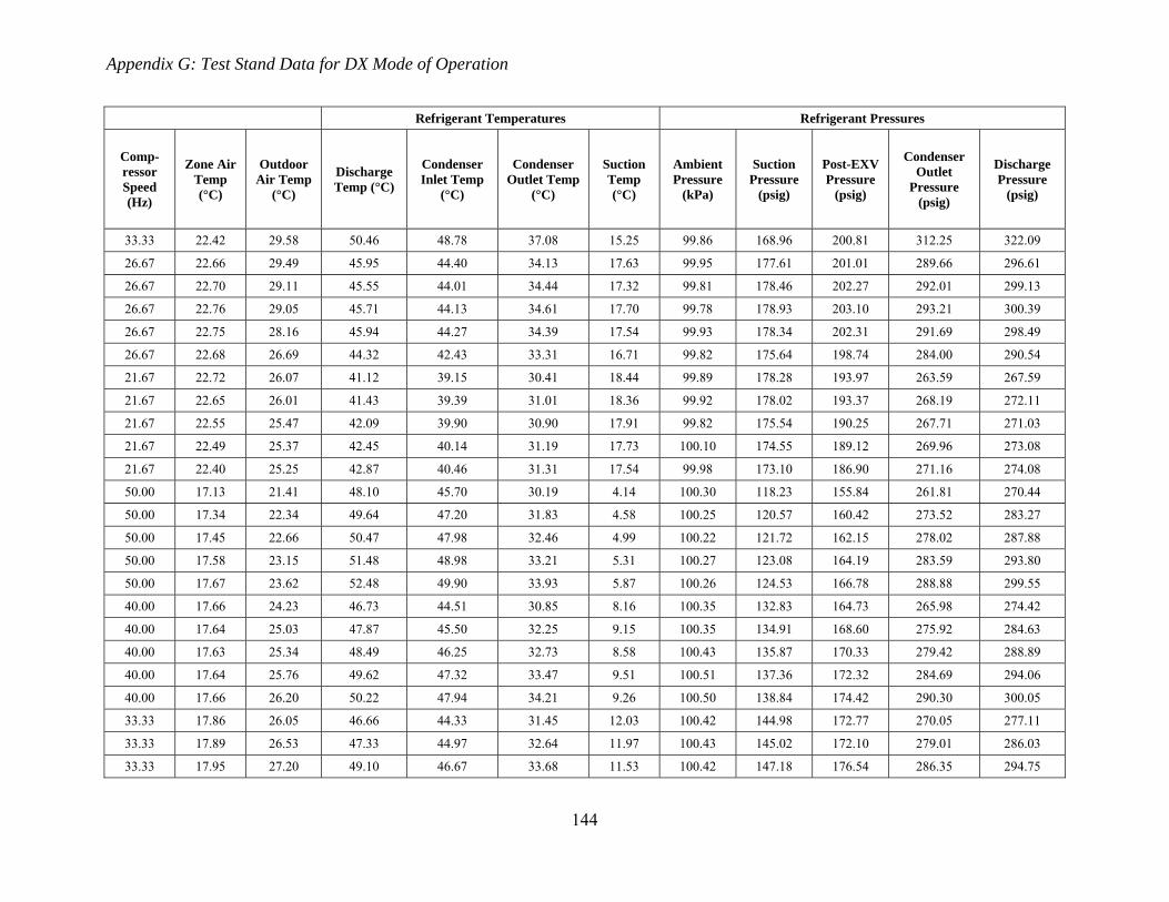
Appendix G: Test Stand Data for DX Mode of Operation
144
Refrigerant Temperatures Refrigerant Pressures
Comp-ressor Speed (Hz)
Zone Air Temp (°C)
Outdoor Air Temp
(°C)
Discharge Temp (°C)
Condenser Inlet Temp
(°C)
Condenser Outlet Temp
(°C)
Suction Temp (°C)
Ambient Pressure
(kPa)
Suction Pressure
(psig)
Post-EXV Pressure
(psig)
Condenser Outlet
Pressure (psig)
Discharge Pressure
(psig)
33.33 22.42 29.58 50.46 48.78 37.08 15.25 99.86 168.96 200.81 312.25 322.09
26.67 22.66 29.49 45.95 44.40 34.13 17.63 99.95 177.61 201.01 289.66 296.61
26.67 22.70 29.11 45.55 44.01 34.44 17.32 99.81 178.46 202.27 292.01 299.13
26.67 22.76 29.05 45.71 44.13 34.61 17.70 99.78 178.93 203.10 293.21 300.39
26.67 22.75 28.16 45.94 44.27 34.39 17.54 99.93 178.34 202.31 291.69 298.49
26.67 22.68 26.69 44.32 42.43 33.31 16.71 99.82 175.64 198.74 284.00 290.54
21.67 22.72 26.07 41.12 39.15 30.41 18.44 99.89 178.28 193.97 263.59 267.59
21.67 22.65 26.01 41.43 39.39 31.01 18.36 99.92 178.02 193.37 268.19 272.11
21.67 22.55 25.47 42.09 39.90 30.90 17.91 99.82 175.54 190.25 267.71 271.03
21.67 22.49 25.37 42.45 40.14 31.19 17.73 100.10 174.55 189.12 269.96 273.08
21.67 22.40 25.25 42.87 40.46 31.31 17.54 99.98 173.10 186.90 271.16 274.08
50.00 17.13 21.41 48.10 45.70 30.19 4.14 100.30 118.23 155.84 261.81 270.44
50.00 17.34 22.34 49.64 47.20 31.83 4.58 100.25 120.57 160.42 273.52 283.27
50.00 17.45 22.66 50.47 47.98 32.46 4.99 100.22 121.72 162.15 278.02 287.88
50.00 17.58 23.15 51.48 48.98 33.21 5.31 100.27 123.08 164.19 283.59 293.80
50.00 17.67 23.62 52.48 49.90 33.93 5.87 100.26 124.53 166.78 288.88 299.55
40.00 17.66 24.23 46.73 44.51 30.85 8.16 100.35 132.83 164.73 265.98 274.42
40.00 17.64 25.03 47.87 45.50 32.25 9.15 100.35 134.91 168.60 275.92 284.63
40.00 17.63 25.34 48.49 46.25 32.73 8.58 100.43 135.87 170.33 279.42 288.89
40.00 17.64 25.76 49.62 47.32 33.47 9.51 100.51 137.36 172.32 284.69 294.06
40.00 17.66 26.20 50.22 47.94 34.21 9.26 100.50 138.84 174.42 290.30 300.05
33.33 17.86 26.05 46.66 44.33 31.45 12.03 100.42 144.98 172.77 270.05 277.11
33.33 17.89 26.53 47.33 44.97 32.64 11.97 100.43 145.02 172.10 279.01 286.03
33.33 17.95 27.20 49.10 46.67 33.68 11.53 100.42 147.18 176.54 286.35 294.75

Appendix G: Test Stand Data for DX Mode of Operation
145
Condenser Conditions Evaporator Conditions Power Measurements
Condenser Air Inlet
Temp (°C)
Condenser Air Temp Difference
(°C)
Evaporator Volumetric Flow Rate (m3/s)
Refrigerant Mass Flow Rate (kg/s)
Compressor Three Phase Power (W)
Fan Three Phase Power
(W)
35.71 3.42 0.158 0.011 171.83 23.21
36.74 3.60 0.158 0.012 177.09 22.78
37.64 3.62 0.158 0.012 181.16 16.44
36.24 5.09 0.158 0.013 230.43 22.78
35.41 5.61 0.158 0.013 226.76 24.32
34.70 6.03 0.158 0.013 224.74 16.81
35.25 7.58 0.158 0.013 238.13 4.30
35.68 7.07 0.158 0.014 316.85 22.62
36.27 7.76 0.158 0.015 330.60 23.78
34.30 8.46 0.158 0.014 321.37 22.51
34.79 9.69 0.158 0.016 432.86 23.60
33.82 10.08 0.158 0.016 426.48 24.52
33.08 10.77 0.158 0.016 425.93 16.21
30.39 6.66 0.158 0.014 381.72 29.61
30.33 6.73 0.158 0.014 386.46 26.33
30.24 5.83 0.158 0.014 383.50 25.99
29.85 6.74 0.158 0.013 391.79 24.27
29.12 9.04 0.158 0.015 528.74 29.35
28.89 8.55 0.158 0.015 536.27 27.46
28.84 8.25 0.158 0.015 536.19 25.80
28.89 8.10 0.158 0.015 534.25 24.64
28.94 8.35 0.158 0.014 450.44 15.94
27.83 6.66 0.158 0.012 265.74 29.77
27.83 7.51 0.158 0.012 271.79 27.30

Appendix G: Test Stand Data for DX Mode of Operation
146
Condenser Conditions Evaporator Conditions Power Measurements
Condenser Air Inlet
Temp (°C)
Condenser Air Temp Difference
(°C)
Evaporator Volumetric Flow Rate (m3/s)
Refrigerant Mass Flow Rate (kg/s)
Compressor Three Phase Power (W)
Fan Three Phase Power
(W)
27.64 7.68 0.158 0.012 270.94 25.71
27.46 7.69 0.158 0.012 273.60 24.60
27.28 7.96 0.158 0.012 273.52 16.09
28.79 9.26 0.158 0.013 501.04 29.06
29.27 10.28 0.158 0.015 524.11 26.21
29.92 10.25 0.158 0.015 520.92 26.09
30.44 10.51 0.158 0.015 534.82 24.89
30.56 10.95 0.158 0.015 541.76 16.31
30.72 7.44 0.158 0.013 366.91 29.01
30.86 8.20 0.158 0.013 377.91 26.44
30.39 8.32 0.158 0.013 376.99 25.12
29.81 8.63 0.158 0.014 380.10 24.29
29.61 8.78 0.158 0.013 379.71 16.28
29.63 5.66 0.158 0.012 272.62 28.94
29.24 6.56 0.158 0.012 279.08 25.89
29.48 6.68 0.158 0.012 281.32 25.31
29.44 6.88 0.158 0.012 282.81 24.20
29.58 7.02 0.158 0.012 284.71 16.02
29.49 4.30 0.158 0.011 191.58 28.79
29.11 4.95 0.158 0.011 192.61 26.17
29.05 5.22 0.158 0.011 193.83 25.74
28.16 5.57 0.158 0.011 192.63 23.93
26.69 6.01 0.158 0.011 185.48 16.25
26.07 3.96 0.158 0.009 133.54 29.38

Appendix G: Test Stand Data for DX Mode of Operation
147
Condenser Conditions Evaporator Conditions Power Measurements
Condenser Air Inlet
Temp (°C)
Condenser Air Temp Difference
(°C)
Evaporator Volumetric Flow Rate (m3/s)
Refrigerant Mass Flow Rate (kg/s)
Compressor Three Phase Power (W)
Fan Three Phase Power
(W)
26.01 4.54 0.158 0.009 138.85 25.80
25.47 4.98 0.158 0.009 140.85 25.12
25.37 5.27 0.158 0.008 144.28 23.66
25.25 5.59 0.158 0.008 146.77 17.19
21.41 7.95 0.158 0.012 401.52 29.36
22.34 8.86 0.158 0.012 420.93 26.21
22.66 9.20 0.158 0.012 427.30 25.37
23.15 9.50 0.158 0.012 435.83 24.61
23.62 9.76 0.158 0.013 443.83 16.40
24.23 6.11 0.158 0.011 308.01 29.42
25.03 6.81 0.158 0.012 320.80 27.06
25.34 6.97 0.158 0.012 326.28 25.49
25.76 7.34 0.158 0.012 332.98 24.00
26.20 7.57 0.158 0.012 339.54 16.92
26.05 4.91 0.158 0.011 248.40 29.21
26.53 5.65 0.158 0.011 260.00 25.56
27.20 5.87 0.158 0.011 269.02 25.09

Appendix H: Test Stand Data for Chiller Mode of Operation
148
Appendix H
14 Test Stand Data for Chiller Mode of Operation
Refrigerant Temperatures Refrigerant pressures
Comp-ressor Speed (Hz)
Condenser Fan Speed
(RPM)
Zone Air Temp (°C)
Outdoor Air
Temp (°C)
Discharge Temp (°C)
Condenser Inlet
Temp (°C)
Condenser Outlet
Temp (°C)
Suction Temp (°C)
Ambient Pressure
(kPa)
Suction Pressure
(psig)
Post-EXV
Pressure (psig)
Condenser Outlet
Pressure (psig)
Discharge Pressure
(psig)
33.33 690.50 27.22 27.85 53.23 50.94 31.92 21.54 98.87 181.37 187.03 318.94 321.29
33.33 502.70 27.10 28.44 56.70 54.26 34.06 21.60 98.87 181.88 187.41 336.12 338.44
33.33 387.50 27.00 28.24 58.64 56.01 35.93 21.64 98.83 181.93 187.43 350.92 353.52
26.67 895.50 26.73 27.49 48.85 46.49 30.00 22.12 99.00 185.06 188.79 301.37 301.87
26.67 686.30 26.69 27.09 50.13 47.69 30.24 22.12 99.02 185.02 188.76 304.79 305.40
26.67 498.70 26.67 28.57 53.05 50.29 32.63 22.19 98.90 185.29 189.06 323.18 323.99
26.67 384.40 26.69 32.28 62.13 58.59 38.03 22.43 99.12 186.64 190.38 365.67 367.04
26.67 889.80 26.78 32.73 57.79 53.89 34.21 17.77 98.98 160.71 163.92 331.01 331.49
26.67 681.20 26.85 33.62 60.85 56.60 35.66 17.94 99.29 161.56 164.70 343.40 343.96
26.67 498.40 26.94 34.56 64.63 59.87 37.74 18.00 99.22 161.94 165.05 361.12 361.55
33.33 898.80 26.69 26.70 51.90 49.13 29.14 17.06 98.97 156.85 161.22 296.98 298.15
33.33 688.20 26.44 26.65 52.85 50.03 29.80 17.06 99.25 156.98 161.23 302.93 304.14
33.33 505.20 26.25 26.75 55.40 52.41 31.10 17.12 98.96 157.18 161.42 313.38 314.73
33.33 389.30 26.05 28.49 60.67 57.24 34.36 16.85 99.13 155.66 159.81 338.42 339.73
33.33 897.75 25.97 27.91 52.12 49.91 30.80 21.29 99.13 180.13 185.19 310.10 312.31
43.33 893.30 27.34 27.82 60.12 57.65 32.69 15.28 98.96 147.79 158.09 327.39 333.39
43.33 685.30 27.18 28.06 62.44 59.85 34.12 15.14 98.93 146.83 157.08 338.71 344.85
43.33 503.80 27.03 28.04 65.41 62.70 36.15 15.31 99.05 147.78 158.24 355.23 361.51
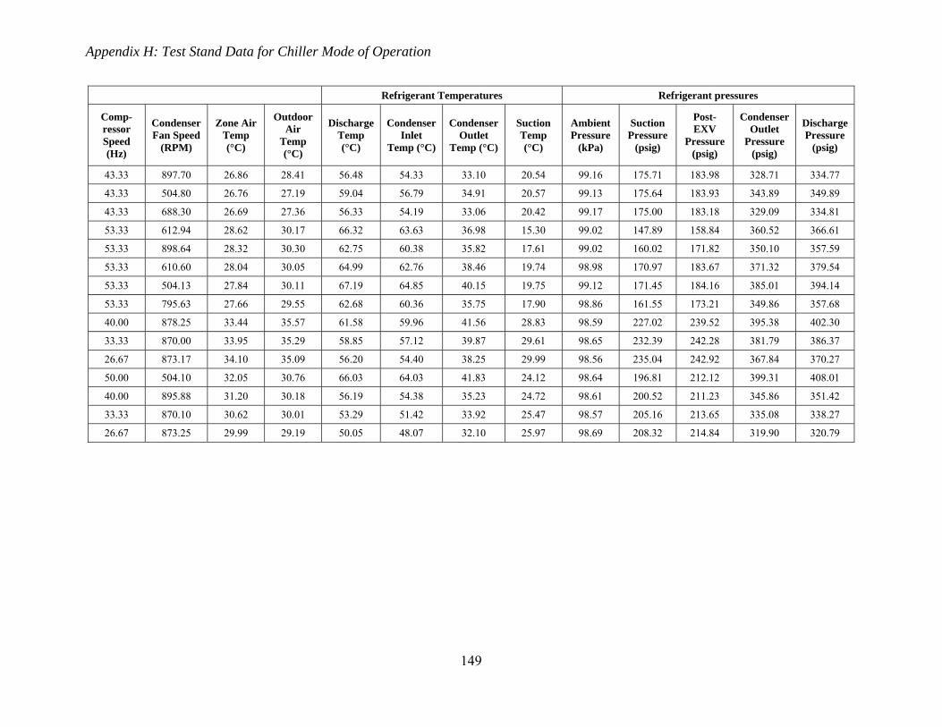
Appendix H: Test Stand Data for Chiller Mode of Operation
149
Refrigerant Temperatures Refrigerant pressures
Comp-ressor Speed (Hz)
Condenser Fan Speed
(RPM)
Zone Air Temp (°C)
Outdoor Air
Temp (°C)
Discharge Temp (°C)
Condenser Inlet
Temp (°C)
Condenser Outlet
Temp (°C)
Suction Temp (°C)
Ambient Pressure
(kPa)
Suction Pressure
(psig)
Post-EXV
Pressure (psig)
Condenser Outlet
Pressure (psig)
Discharge Pressure
(psig)
43.33 897.70 26.86 28.41 56.48 54.33 33.10 20.54 99.16 175.71 183.98 328.71 334.77
43.33 504.80 26.76 27.19 59.04 56.79 34.91 20.57 99.13 175.64 183.93 343.89 349.89
43.33 688.30 26.69 27.36 56.33 54.19 33.06 20.42 99.17 175.00 183.18 329.09 334.81
53.33 612.94 28.62 30.17 66.32 63.63 36.98 15.30 99.02 147.89 158.84 360.52 366.61
53.33 898.64 28.32 30.30 62.75 60.38 35.82 17.61 99.02 160.02 171.82 350.10 357.59
53.33 610.60 28.04 30.05 64.99 62.76 38.46 19.74 98.98 170.97 183.67 371.32 379.54
53.33 504.13 27.84 30.11 67.19 64.85 40.15 19.75 99.12 171.45 184.16 385.01 394.14
53.33 795.63 27.66 29.55 62.68 60.36 35.75 17.90 98.86 161.55 173.21 349.86 357.68
40.00 878.25 33.44 35.57 61.58 59.96 41.56 28.83 98.59 227.02 239.52 395.38 402.30
33.33 870.00 33.95 35.29 58.85 57.12 39.87 29.61 98.65 232.39 242.28 381.79 386.37
26.67 873.17 34.10 35.09 56.20 54.40 38.25 29.99 98.56 235.04 242.92 367.84 370.27
50.00 504.10 32.05 30.76 66.03 64.03 41.83 24.12 98.64 196.81 212.12 399.31 408.01
40.00 895.88 31.20 30.18 56.19 54.38 35.23 24.72 98.61 200.52 211.23 345.86 351.42
33.33 870.10 30.62 30.01 53.29 51.42 33.92 25.47 98.57 205.16 213.65 335.08 338.27
26.67 873.25 29.99 29.19 50.05 48.07 32.10 25.97 98.69 208.32 214.84 319.90 320.79

Appendix H: Test Stand Data for Chiller Mode of Operation
150
Condenser Conditions Evaporator Conditions Power Measurements
Condenser Air Inlet
Temp (°C)
Condenser Air Temp Difference
(°C)
Evaporator Inlet Temp
(°C)
Evaporator Outlet
Temp (°C)
Water Inlet
Temp (°C)
Water Outlet
Temp (°C)
Water Volumetric Flow Rate
(L/s)
Refrigerant Mass Flow Rate (kg/s)
Cooling Load (W)
Compressor Three Phase
Power (W)
Fan Three Phase Power
(W)
Pump Power
(W)
27.85 5.10 16.51 21.19 22.22 20.08 0.268 0.015 2464.84 276.03 18.73 22.89
28.44 7.17 16.69 21.25 22.18 20.11 0.270 0.015 2378.82 301.81 6.22 22.91
28.24 9.46 16.74 21.29 22.13 20.11 0.272 0.015 2322.96 323.32 2.61 22.91
27.49 3.19 16.77 21.68 22.26 20.45 0.272 0.013 2039.09 193.66 46.24 23.05
27.09 4.21 16.80 21.58 22.19 20.40 0.272 0.012 2034.36 199.23 18.72 23.05
28.57 5.84 16.96 21.62 22.19 20.46 0.268 0.012 1959.47 222.17 6.03 23.09
32.28 7.59 17.44 21.73 22.24 20.68 0.272 0.012 1755.68 282.06 2.66 23.07
32.73 2.55 12.66 16.80 17.21 15.95 0.261 0.010 1569.85 258.87 45.26 23.03
33.62 3.38 12.85 16.71 17.16 15.95 0.260 0.010 1525.97 274.84 18.62 23.00
34.56 4.73 12.96 16.68 17.11 15.97 0.259 0.010 1450.65 302.87 6.51 22.98
26.70 3.39 11.85 16.41 17.14 15.28 0.260 0.013 2139.53 270.31 46.42 22.60
26.65 4.47 11.90 16.37 17.11 15.26 0.260 0.013 2128.38 279.43 18.86 22.60
26.75 6.24 11.97 16.38 17.09 15.29 0.260 0.013 2080.77 296.73 6.36 22.60
28.49 8.05 11.76 16.01 16.63 14.95 0.260 0.012 1940.06 330.09 2.63 22.60
27.91 3.75 16.14 21.06 22.04 19.74 0.260 0.015 2496.06 263.51 46.61 22.60
27.82 5.23 11.01 15.18 17.44 14.75 0.260 0.019 3118.56 528.35 45.98 22.60
28.06 6.82 10.83 15.34 17.09 14.48 0.260 0.019 3032.27 553.08 18.71 22.60
28.04 9.51 11.06 15.57 17.15 14.61 0.260 0.019 2955.56 588.13 6.30 22.60
28.41 4.90 15.88 20.95 22.27 19.50 0.260 0.019 3070.34 389.20 46.29 22.60
27.19 9.02 15.94 20.97 22.13 19.45 0.260 0.018 2977.50 418.61 6.47 22.60
27.36 6.44 15.73 20.84 22.13 19.35 0.260 0.018 3056.03 393.04 18.88 22.60
30.17 7.64 11.20 15.41 17.21 14.75 0.260 0.019 2923.53 600.57 12.35 22.60
30.30 5.50 13.52 17.76 20.05 17.19 0.260 0.021 3285.24 566.31 46.31 22.60
30.05 8.74 15.70 20.21 22.29 19.28 0.260 0.022 3401.19 599.87 12.29 22.60
30.11 10.70 15.82 20.14 22.23 19.29 0.260 0.022 3328.37 630.00 6.28 22.60
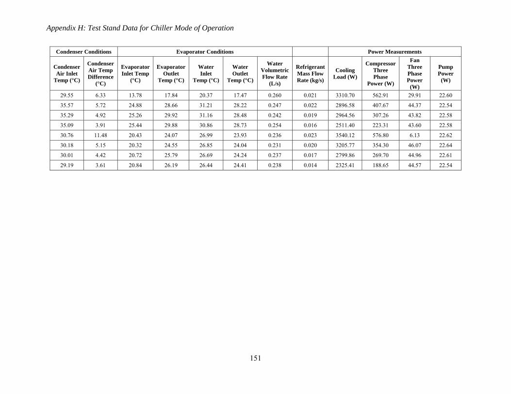
Appendix H: Test Stand Data for Chiller Mode of Operation
151
Condenser Conditions Evaporator Conditions Power Measurements
Condenser Air Inlet
Temp (°C)
Condenser Air Temp Difference
(°C)
Evaporator Inlet Temp
(°C)
Evaporator Outlet
Temp (°C)
Water Inlet
Temp (°C)
Water Outlet
Temp (°C)
Water Volumetric Flow Rate
(L/s)
Refrigerant Mass Flow Rate (kg/s)
Cooling Load (W)
Compressor Three Phase
Power (W)
Fan Three Phase Power
(W)
Pump Power
(W)
29.55 6.33 13.78 17.84 20.37 17.47 0.260 0.021 3310.70 562.91 29.91 22.60
35.57 5.72 24.88 28.66 31.21 28.22 0.247 0.022 2896.58 407.67 44.37 22.54
35.29 4.92 25.26 29.92 31.16 28.48 0.242 0.019 2964.56 307.26 43.82 22.58
35.09 3.91 25.44 29.88 30.86 28.73 0.254 0.016 2511.40 223.31 43.60 22.58
30.76 11.48 20.43 24.07 26.99 23.93 0.236 0.023 3540.12 576.80 6.13 22.62
30.18 5.15 20.32 24.55 26.85 24.04 0.231 0.020 3205.77 354.30 46.07 22.64
30.01 4.42 20.72 25.79 26.69 24.24 0.237 0.017 2799.86 269.70 44.96 22.61
29.19 3.61 20.84 26.19 26.44 24.41 0.238 0.014 2325.41 188.65 44.57 22.54

Appendix I: Nomenclature
152
Appendix I
15 Nomenclature
A Area (m) n Polytropic exponent
cp Specific heat (J/kg.K) n Isentropic exponent
D Tube inside diameter (m) P Pressure (kPa)
D Tube outside diameter (m) Pf Heat exchanger fin pitch
D Collar diameter (m) D D 2
tf
P Longitudinal pitch of heat exchanger
dP Pressure drop P Transversal pitch of heat exchanger
e Void fraction Pr Prandtl number Pr µ cp/k
Fr Froude number Q Heat (W)
f Friction factor Q Evaporator heat load (W)
f Compressor speed (Hz) qf Heat flux QF Q/A (W/m2)
G Mass velocity or mass flux (G m/
A) (kg/s.m2)
RMSE Root Mean Squared Error
RMSE ∑ P AD P
h Specific enthalpy (J/kg) Re Reynolds number (R G D/µ)
h Single-phase convection heat transfer
coefficient (W/m2.K)
R Equivalent radius (m)
h Air-side heat transfer coefficient
(W/m2.K)
r Tube radius (m)
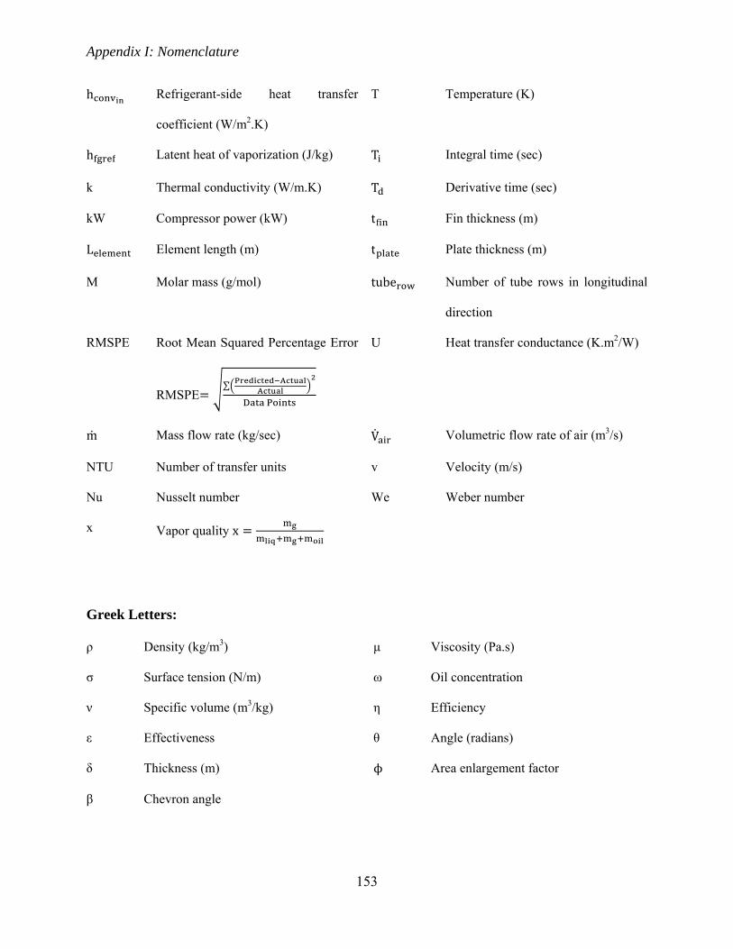
Appendix I: Nomenclature
153
h Refrigerant-side heat transfer
coefficient (W/m2.K)
T Temperature (K)
h Latent heat of vaporization (J/kg) T Integral time (sec)
k Thermal conductivity (W/m.K) T Derivative time (sec)
kW Compressor power (kW) tf Fin thickness (m)
L Element length (m) t Plate thickness (m)
M Molar mass (g/mol) tube Number of tube rows in longitudinal
direction
RMSPE Root Mean Squared Percentage Error
RMSPE∑ P A
AD P
U Heat transfer conductance (K.m2/W)
m Mass flow rate (kg/sec) V Volumetric flow rate of air (m3/s)
NTU Number of transfer units v Velocity (m/s)
Nu Nusselt number We Weber number
x Vapor quality x
Greek Letters:
ρ Density (kg/m3) μ Viscosity (Pa.s)
σ Surface tension (N/m) ω Oil concentration
ν Specific volume (m3/kg) η Efficiency
ε Effectiveness θ Angle (radians)
δ Thickness (m) Area enlargement factor
β Chevron angle

Appendix I: Nomenclature
154
Sub-scripts:
amb Ambient max Maximum
bulb Saturation temperature of refrigerant-oil
mixture
min Minimum
comb Combined min Element area exposed to air
cond Condenser oil Refrigerant oil POE/VG68
cond Condenser outlet out Output from element
comp Compressor plate Brazed-Plate heat exchanger
crit Critical port Brazed-Plate HX inlet/outlet port
dis Discharge ref Refrigerant
evap Evaporator ref Liquid phase of refrigerant
evap Evaporator inlet ref Gas phase of refrigerant
evap Evaporator outlet ref-oil Refrigerant-oil mixture
eq Equivalent sat Saturation
fin Heat exchanger fins strat Stratified
g Gas suc Suction
gD Gas portion of tube in two-phase surf Surface
IA Intermittent-annular surf Element surface area exposed to air
in Input to the element tp Two-phase
liq Liquid tube Tube of fan-coil heat exchanger
liqD Liquid portion of tube in two-phase v Volumetric
liqfilm Liquid film in two-phase x Outdoor
local Local oil concentration z Indoor

Bibiliography
155
16 Bibliography
Ali, M. T., Mokhtar, M., Chiesa, M., & Armstrong, P. (2011). A cooling change-point model of
community-aggregate electrical load. Energy and Buildings, 43(1), 28-37.
Allen, J. J., & Hamilton, J. F. (1983). Steady-state reciprocating water chiller models. ASHRAE
Transactions, 89(2A), 398–407.
Armstrong, P. R., Jiang, W., Winiarski, D., Katipamula, S., & Norford, L. K. (2009). Efficient
low-lift cooling with radiant distribution, thermal storage, and variable-speed chiller
controls—Part II: Annual use and energy savings. HVAC&R Research, 15(2), 402–432.
Armstrong, P. R., Jiang, W., Winiarski, D., Katipamula, S., Norford, L. K., & Willingham, R. A.
(2009). Efficient low-lift cooling with radiant distribution, thermal storage, and variable-
speed chiller controls—Part I: Component and subsystem models. HVAC&R Research,
15(2), 366–401.
Arslan Khalid. (2011). Personal Communication.
Ayub, Z. H. (2003). Plate heat exchanger literature survey and new heat transfer and pressure
drop correlations for refrigerant evaporators. Heat transfer engineering, 24(5), 3–16.
Bandarra Filho, E. P., Cheng, L., & Thome, J. R. (2009). Flow boiling characteristics and flow
pattern visualization of refrigerant/lubricant oil mixtures. International Journal of
Refrigeration, 32(2), 185–202.
Bendapudi, S., & Braun, J. E. (2002). A review of literature on dynamic models of vapor
compression equipment. ASHRAE Report, HL 2002-9 Report #4036-5.

Bibiliography
156
Boissieux, X., Heikal, M. R., & Johns, R. A. (2000a). Two-phase heat transfer coefficients of
three HFC refrigerants inside a horizontal smooth tube—Part II: Condensation.
International Journal of Refrigeration, 23(5), 345-352.
Boissieux, X., Heikal, M. R., & Johns, R. A. (2000b). Two-phase heat transfer coefficients of
three HFC refrigerants inside a horizontal smooth tube—Part I: Evaporation.
International Journal of Refrigeration, 23(4), 269-283.
Brown, R. N. (1997). Compressors: Selection and Sizing. Gulf Professional Publishing.
Browne, M. W., & Bansal, P. K. (2001). An elemental NTU-model for vapor-compression liquid
chillers. International Journal of Refrigeration, 24(7), 612–627.
Cavallini, A., Censi, G., Del Col, D., Doretti, L., Longo, G. A., & Rossetto, L. (2002). In-tube
condensation of halogenated refrigerants. ASHRAE Transactions, 108(4507), 146–161.
Chen, I. Y., Wang, C.-C., & Lin, S. Y. (2004). Measurements and correlations of frictional
single-phase and two-phase pressure drops of R-410A flow in small U-type return bends.
International Journal of Heat and Mass Transfer, 47(10-11), 2241-2249.
Chen, I. Y., Wu, Y.-S., Chang, Y.-J., & Wang, C.-C. (2007). Two-phase frictional pressure drop
of R-134a and R-410A refrigerant-oil mixtures in straight tubes and U-type wavy tubes.
Experimental Thermal and Fluid Science, 31(4), 291-299.
Cho, K., & Tae, S.-J. (2001). Condensation heat transfer for R-22 and R-407C refrigerant-oil
mixtures in a micro-fin tube with a U-bend. International Journal of Heat and Mass
Transfer, 44(11), 2043-2051.
Choi, J. Y., Kedzierski, M. A., & Domański, P. (1999). A generalized pressure drop correlation
for evaporation and condensation of alternative refrigerants in smooth and micro-fin

Bibiliography
157
tubes. US Dept. of Commerce, Technology Administration, National Institute of
Standards and Technology, Building and Fire Research Laboratory.
Claesson, J. (2005). Thermal and hydraulic performance of compact brazed plate heat
exchangers operating as evaporators in domestic heat pumps (Ph.D. thesis). KTH,
Sweden: Royal Institute of Technology.
Cohen, R., Hamilton, J. F., & Pearson, J. T. (1974). Possible energy conservation through the use
of variable capacity compressor. Proceedings Purdue Compressor Technology
Conference, Purdue, US (pp. 50–55).
Conde, M. R. (1996). Estimation of thermophysical properties of lubricating oils and their
solutions with refrigerants: an appraisal of existing methods. Applied thermal
engineering, 16(1), 51–61.
Cooper, M. G. (1984). Heat flow rates in saturated nucleate pool boiling-a wide-ranging
examination using reduced properties. Advances in heat transfer, 16, 157–239.
Damasceno, G. S., Goldschmidt, V. W., & Rooke, S. P. (1990). Comparison of three steady-state
heat pump computer models. ASHRAE Transactions, 96(2), 191–204.
Doerr, T. M., Pate, M. B., & Eckels, S. J. (1994). In-tube heat transfer and pressure drop of R-
134a and ester lubricant mixtures in a smooth tube and a micro-fin tube: part I -
evaporation. ASHRAE Transactions, 100(2), 265-282.
Domanski, P., & Didion, D. (1984). Mathematical model of an air-to-air heat pump equipped
with a capillary tube. International Journal of Refrigeration, 7(4), 249–255.
El Hajal, J., Thome, J. R., & Cavallini, A. (2003). Condensation in horizontal tubes, part 1: two-
phase flow pattern map. International Journal of Heat and Mass Transfer, 46(18), 3349–
3363.

Bibiliography
158
Feustel, H. E., & Stetiu, C. (1995). Hydronic radiant cooling–preliminary assessment. Energy
and buildings, 22(3), 193–205.
Fischer, S. K., Rice, C. K., & Jackson, W. L. (1988). The Oak Ridge Heat Pump Design Model:
Mark III Version Program Documentation. ORNL/TM-10192.
Friedel, L. (1979). Improved friction pressure drop correlations for horizontal and vertical two-
phase pipe flow. European two-phase flow group meeting, Paper E (Vol. 2).
Fukuta, M., Yanagisawa, T., Miyamura, S., & Ogi, Y. (2004). Concentration measurement of
refrigerant/refrigeration oil mixture by refractive index. International Journal of
Refrigeration, 27(4), 346-352.
García-Cascales, J. R., Vera-García, F., Corberán-Salvador, J. M., & Gonzálvez-Maciá, J.
(2007). Assessment of boiling and condensation heat transfer correlations in the
modelling of plate heat exchangers. International Journal of Refrigeration, 30(6), 1029–
1041.
Gayeski, N. T. (2010). Predictive pre-cooling control for low lift radiant cooling using building
thermal mass. (PhD Thesis). Massachusetts Institute of Technology.
Gayeski, N. T., Zakula, T., Armstrong, P. R., & Norford, L. K. (2010). Empirical Modeling of a
Rolling-Piston Compressor Heat Pump for Predictive Control in Low Lift Cooling.
ASHRAE Transactions, 116(1).
Gnielinski, V. (1976). New equations for heat and mass transfer in turbulent pipe and channel
flow. Int. Chem. Eng, 16(2), 359–368.
Gray, D. L., & Webb, R. L. (1986). Heat transfer and friction correlations for plate finned-tube
heat exchangers having plain fins. Proceedings of the 8th International Heat Transfer
Conference (Vol. 6, pp. 2745–2750).

Bibiliography
159
Grönnerud, R. (1972). Investigation of Liquid Hold-Up, Flow-Resistance and Heat Transfer in
Circulation Type Evaporators, Part IV: Two-Phase Flow Resistance in Boiling
Refrigerants. Bull. De l’Inst. Du Froid, Annexe, 1.
Hambraeus, K. (1995). Heat transfer of oil-contaminated HFC134a in a horizontal evaporator.
International Journal of Refrigeration, 18(2), 87-99.
Hamilton, J. F., & Miller, J. L. (1990). A simulation program for modeling an air-conditioning
system. ASHRAE Transactions, 96(1), 213–221.
Han, D. H., Lee, K. J., & Kim, Y. H. (2003). Experiments on the characteristics of evaporation
of R410A in brazed plate heat exchangers with different geometric configurations.
Applied thermal engineering, 23(10), 1209–1225.
Harp Lubricants – Technical Data SheetHarp Polyol Ester Oils. Harp International.
Hermetic Compressors. (2011). . Retrieved May 3, 2011, from
http://www.refrigers.com/content/view/31439/28/
Hiller, C. C., & Glicksman, L. R. (1976). Improving heat pump performance via compressor
capacity control: analysis and test. MIT Energy Lab.
Hsieh, Y. Y., & Lin, T. F. (2002). Saturated flow boiling heat transfer and pressure drop of
refrigerant R-410A in a vertical plate heat exchanger. International journal of heat and
mass transfer, 45(5), 1033–1044.
Hsieh, Y. Y., & Lin, T. F. (2003). Evaporation heat transfer and pressure drop of refrigerant R-
410A flow in a vertical plate heat exchanger. Journal of heat transfer, 125, 852.
Hu, H., Ding, G., Wei, W., Wang, Z., & Wang, K. (2008). Heat transfer characteristics of
R410A-oil mixture flow boiling inside a 7 mm straight smooth tube. Experimental
Thermal and Fluid Science, 32(3), 857–869.

Bibiliography
160
Iu, I. S. (2007). Development of air-to-air heat pump simulation program with advanced heat
exchanger circuitry algorithm. Oklahoma State University.
Jacobi, A. M., Park, Y., Tafti, D., & Zhang, X. (2001). An Assessment of The State of The Art,
And Potential Design Improvements, For Flat-Tube Heat Exchangers In Air
Conditioning And Refrigeration Applications-Phase I. Air-Conditioning and
Refrigeration Technology Institute, Arlington, VA (US).
Jähnig, D. I., Reindl, D. T., & Klein, S. A. (2000). A semi-empirical method for representing
domestic refrigerator/freezer compressor calorimeter test data. ASHRAE Transactions,
106(4379 (RP-870)), 122–30.
Jeong, J., Kim, C. N., & Youn, B. (2006). A study on the thermal contact conductance in fin-tube
heat exchangers with 7 mm tube. International Journal of Heat and Mass Transfer, 49(7-
8), 1547-1555.
Jin, H., & Spitler, J. D. (2002). A parameter estimation based model of water-to-water heat
pumps for use in energy calculation programs. ASHRAE Transactions, 108(4493), 3–17.
Lebreton, J. M., Vuillame, L., Morvan, E., & Lottin, O. (2001). Oil Concentration Measurement
In Saturated Liquid Refrigerant Flowing Inside A Refrigeration Machine. International
Journal of Applied Thermodynamics, 4(1), 53-60.
Lida, K., Yamamoto, T., Kuroda, T., & Hibi, H. (1982). Development of an energy saving
oriented variable capacity system heat pump. ASHRAE Transactions, 88(DA-88-6-4),
441–449.
Martin, H. (1996). A theoretical approach to predict the performance of chevron-type plate heat
exchangers. Chemical Engineering and Processing, 35(4), 301-310.

Bibiliography
161
Michael D. Larrañaga, Mario G. Beruvides, H.W. Holder, Enusha Karunasena, & David C.
Straus. (2008). DOAS & Humidity Control. ASHRAE Journal, 34-40.
Moreno Quibén, J., & Thome, J. R. (2007a). Flow pattern based two-phase frictional pressure
drop model for horizontal tubes, Part II: New phenomenological model. International
Journal of Heat and Fluid Flow, 28(5), 1060–1072.
Moreno Quibén, J., & Thome, J. R. (2007b). Flow pattern based two-phase frictional pressure
drop model for horizontal tubes, Part II: New phenomenological model. International
Journal of Heat and Fluid Flow, 28(5), 1060–1072.
Muley, A., & Manglik, R. M. (1999). Experimental study of turbulent flow heat transfer and
pressure drop in a plate heat exchanger with chevron plates. Journal of heat transfer, 121,
110.
Nidegger, E., Thome, J. R., & Favrat, D. (1997). Flow boiling andpressure drop measurements
for R134a/oil mixtures part 1:evaporation in a microfin tube. HVAC&R Research, 3(1),
38-53.
Niu, J. L., Zhang, L. Z., & Zuo, H. G. (2002). Energy savings potential of chilled-ceiling
combined with desiccant cooling in hot and humid climates. Energy and Buildings, 34(5),
487–495.
Perrotin, T., & Clodic, D. (2003). Fin efficiency calculation in enhanced fin-and-tube heat
exchangers in dry conditions. International Congress of Refrigeration.
Qureshi, T. Q., & Tassou, S. A. (1996). Variable-speed capacity control in refrigeration systems.
Applied Thermal Engineering, 16(2), 103–113.

Bibiliography
162
Radhi, H. (2009). Evaluating the potential impact of global warming on the UAE residential
buildings-A contribution to reduce the CO2 emissions. Building and Environment,
44(12), 2451–2462.
Rice, C. K. (1988). Efficiency Characteristics of Speed Modulated Drives at Predicted Torque
Conditions for Air-to-Air Heat Pumps. ASHRAE Transactions, 94(DA-88-6-4), 892-921.
Roth, K. W., Westphalen, D., Dieckmann, J., Hamilton, S. D., & Goetzler, W. (2002). Energy
consumption characteristics of commercial building hvac systems–volume III: energy
savings potential. Final Report by TIAX LLC to US Department of Energy, Office of
Building Technology, State and Community Programs.
Sarntichartsak, P., Monyakul, V., Thepa, S., & Nathakaranakule, A. (2006). Simulation and
experimental evaluation of the effects of oil circulation in an inverter air conditioning
system using R-22 and R-407C. Applied Thermal Engineering, 26(14-15), 1481-1491.
Schmidt, T. E. (1949). Heat transfer calculations for extended surfaces. Refrigerating
Engineering, 57, 351–357.
Shah, M. M. (1979). A general correlation for heat transfer during film condensation inside
pipes. International Journal of Heat and Mass Transfer, 22(4), 547–556.
Shen, B., & Groll, E. A. (2005). A Critical Review of the Influence of Lubricants on the Heat
Transfer and Pressure Drop of Refrigerants-Part II: Lubricant Influence on Condensation
and Pressure Drop. HVAC&R Research, 11(4), 511.
Shimma, Y., Tateuchi, T., & Sugiura, H. (1985). Inverter control systems in the residential heat
pump air conditioner. ASHRAE Transactions, 91(HI-85-31).
Stefanuk, N. B. M., Aplevich, J. D., & Renksizbulut, M. (1993). Modeling and simulation of a
superheat-controlled water-to-water heat pump. ASHRAE Transactions, 98, 172–172.

Bibiliography
163
Tcheou, E., & McNeil, D. A. (1994). The effect of ester-oils on heattransfer during evaporation
of refrigerant HFC134a. Proceedings of the 10th International Heat Transfer Conference
(pp. 551-556). Brighton, UK.
The benefits of Aluminum in HVAC&R Heat Exchangers. (2011). Sapa Heat Transfer.
Thermal Conductivity of some common Materials. (2011). . Retrieved March 5, 2011, from
http://www.engineeringtoolbox.com/thermal-conductivity-d_429.html
Thome, J. R. (2004). Wolverine Engineering Data Book III. Wolverine Tube Inc.
Thome, J. R., El Hajal, J., & Cavallini, A. (2003). Condensation in horizontal tubes, part 2: new
heat transfer model based on flow regimes. International Journal of Heat and Mass
Transfer, 46(18), 3365–3387.
Thome, J. R. (2011). Personal Communication.
Tran, T. N. (1998). Pressure drop and heat transfer study of two-phase flow in small channels.
(PhD Thesis). Texas Tech University.
Tribbe, C., & Müller-Steinhagen, H. M. (2000). An evaluation of the performance of
phenomenological models for predicting pressure gradient during gas-liquid flow in
horizontal pipelines. International Journal of Multiphase Flow, 26(6), 1019-1036.
US Department of Energy. (2010). Buildings Energy Data Book. US Department of Energy.
Wanniarachchi, A. S., Ratnam, U., Tilton, B. E., & Dutta-Roy, K. (1995). Approximate
correlations for chevron-type plate heat exchangers. ASME-PUBLICATIONS-HTD, 314,
145–152.
Wei, W., Ding, G., Hu, H., & Wang, K. (2008). Models of thermodynamic and transport
properties of POE VG68 and R410A/POE VG68 mixture. Frontiers of Energy and
Power Engineering in China, 2(2), 227–234.

Bibiliography
164
Willingham, R. A. (2009). Testing and modeling of compressors for low-lift cooling
applications.
Wojtan, L. (2005). Experimental and analytical investigation of void fraction and heat transfer
during evaporation in horizontal tubes (PhD Thesis).
Wojtan, L., Ursenbacher, T., & Thome, J. R. (2005a). Investigation of flow boiling in horizontal
tubes: Part I–A new diabatic two-phase flow pattern map. International journal of heat
and mass transfer, 48(14), 2955–2969.
Wojtan, L., Ursenbacher, T., & Thome, J. R. (2005b). Investigation of flow boiling in horizontal
tubes: Part II–Development of a new heat transfer model for stratified-wavy, dryout and
mist flow regimes. International journal of heat and mass transfer, 48(14), 2970–2985.
World Building Council for Sustainable Development (WBCSD). (2008). Energy Efficiency in
Buildings. World Building Council for Sustainable Development (WBCSD).
Youbi-Idrissi, M., & Bonjour, J. (2008). The effect of oil in refrigeration: Current research issues
and critical review of thermodynamic aspects. International Journal of Refrigeration,
31(2), 165-179.
Zakula, T. (2011). Personal Communication.
Zakula, T. (2010). Heat pump simulation model and optimal variable-speed control for a wide
range of cooling conditions.
Zürcher, O., Thome, J. R., & Favrat, D. (1997). Flow boiling andpressure drop measurements for
R134a/oil mixtures part 1:evaporation in a plain tube. HVAC&R Research, 3(1), 54-64.