Modeling and Investigation of Refrigeration System

Marquette Universitye-Publications@Marquette

Master's Theses (2009 -) Dissertations, Theses, and Professional Projects

Modeling and Investigation of Refrigeration SystemPerformance with Two-Phase Fluid Injection in aScroll CompressorRui GuMarquette University

Recommended CitationGu, Rui, "Modeling and Investigation of Refrigeration System Performance with Two-Phase Fluid Injection in a Scroll Compressor"(2016). Master's Theses (2009 -). Paper 357.http://epublications.marquette.edu/theses_open/357

http://epublications.marquette.edu

http://epublications.marquette.edu/theses_open

http://epublications.marquette.edu/diss_theses

MODELING AND INVESTIGATION OF REFRIGERATION SYSTEM PERFORMANCE WITH

TWO-PHASE FLUID INJECTION IN A SCROLL COMPRESSOR

By Rui Gu

A Thesis Submitted to the Faculty of the

Graduate School, Marquette University,

in Partial Fulfillment of the Requirements for the

Degree of Master of Science

Milwaukee, Wisconsin

May 2016

PREFACE

MODELING AND INVESTIGATION OF REFRIGERATION SYSTEM PERFORMANCE WITH TWO-PHASE FLUID INJECTION IN A SCROLL

COMPRESSOR

Rui Gu

Under the supervision of Professor Hyunjae Park

and Professor Anthony Bowman

Marquette University, 2016

to circulate and to have copied for non-commercial purposes, at its

discretion, the above title upon the request of individuals or institutions.

To My Parents and Friends

i

ABSTRACT

MODELING AND INVESTIGATION OF REFRIGERATION SYSTEM PERFORMANCE WITH TWO-PHASE FLUID INJECTION IN A SCROLL

COMPRESSOR

Rui Gu Marquette University, 2016

Vapor compression cycles are widely used in heating, refrigerating and air-

conditioning. A slight performance improvement in the components of a vapor

compression cycle, such as the compressor, can play a significant role in saving

energy use. How- ever, the complexity and cost of these improvements can block

their application in the market. Modifying the conventional cycle configuration can

offer a less complex and less costly alternative approach. Economizing is a common

modification for improving the performance of the refrigeration cycle, resulting in

decreasing the work required to compress the gas per unit mass. Traditionally,

economizing requires multi-stage compressors, the cost of which has restrained the

scope for practical implementation. Compressors with injection ports, which can be

used to inject economized refrigerant during the compression process, introduce

new possibilities for economization with less cost. This work focuses on

computationally investigating a refrigeration system performance with two-phase

fluid injection, developing a better understanding of the impact of injected

refrigerant quality on a refrigeration system performance as well as evaluating the

potential COP improvement that injection provides based on refrigeration system

performance provided by Copeland.

ii

ACKNOWLEDGMENTS

Rui Gu Marquette University, 2016

I would like to express my emotions in a chronological order.

I was also so fortunate to work with Dr. Mathison, my first foreign advisor,

during my time at Marquette. Thank you for guiding me through the early years

of chaos and confusions, for sparking my interest in the thermal sciences, and for

encouraging and supporting me to insist on my research career. I appreciate all the

opportunities that you have provided me, and the time you have spent on me.

After that, I was so sorry that she had to leave Marquette for her hometown due to

her family issues. I understood her situation well and prayed for her family, but I

faced the dilemma in my life. Graduated as MS degree or continue my Ph.D. work

by myself?

I was so lucky to meet Dr. Park, my current supervisor and Dr. Bowman,

my favorite professor to help me walk through the difficult situation. I decided to

switch to the MS degree following their advice and recommendations at last. I

appreciated their guidances and supports they had given at that time. I cannot

thank you enough for all you have done when I am trapped in. Now I feel satisfied

about my situation.

Dr. Park found this relevant master project for me based on my previous

research, pictured the panorama of my new program and held the right research

direction. Dr. Bowman expressed his interest in my work as well and supplied me

iii

a perspective on my own results. He shared with me his knowledge and provided

many useful references and friendly encouragement. I appreciate all the efforts you

have made for my project.

I would also like to thank all my friends. They are wonderful people. I

appreciate all the support and friendship that I have received.

Finally, I would not be where I am today without the help of my family.

Thank you to my parents for your love. You have always been there to help and

support me, no matter what kind of situations. Thank you for believing in me and

for always supporting me to pursuing my dreams.

iv

Table of Contents

Abstract i

Acknowledgments ii

List of Tables vii

List of Figures viii

1 Introduction 1

1.1 Background . . . . . . . . . . . . . . . . . . . . . . . . . . . . . . . . 1

1.2 Problem Statement . . . . . . . . . . . . . . . . . . . . . . . . . . . . 2

1.3 Objective . . . . . . . . . . . . . . . . . . . . . . . . . . . . . . . . . 3

1.4 Literature Survey . . . . . . . . . . . . . . . . . . . . . . . . . . . . . 5

2 Analysis of Refrigeration System Based on a Copeland Scroll Com-

pressor Performance Data 9

2.1 Conventional Vapor Refrigeration Cycle . . . . . . . . . . . . . . . . . 9

2.1.1 Introduction of the System . . . . . . . . . . . . . . . . . . . . 9

2.1.2 Thermodynamic Analysis of the System ......................................... 11

2.1.3 Model of The System ......................................................................... 13

2.1.4 Sample Calculation .............................................................................. 14

2.2 Compressor Selection and Copeland Compressor Testing Cycle ............. 18

2.3 Model Results ................................................................................................... 21

2.3.1 Correlation between Compressor Efficiency and Compression

Pressure Ratio .................................................................................... 21

2.3.2 Correlation between Mass Flow Rate and Evaporating Temper-

ature ...................................................................................................... 25

v

2.3.3 Performance Analysis of the Refrigeration Cycle ........................... 26

3 Prediction of the Refrigeration System Performance with Controlled

Injection Pressure 29

3.1 Introduction to Vapor Injection Refrigeration Systems ........................... 29

3.2 Refrigeration System Injected with Isenthalpic Expansion Quality Cor-

responding to Injection Pressure ................................................................. 31

3.2.1 Thermodynamic Analysis of the System ......................................... 31

3.2.2 Model of the System .......................................................................... 34

3.2.3 Sample Calculation and Model Feasibility Analysis ...................... 38

3.2.4 Pre-Simulation Work ................................................................................ 45

3.3 Model Results .................................................................................................. 46

3.3.1 Case Study of Minimum Compressor Efficiency Group ............... 46

3.3.2 Case Study of Maximum Compressor Efficiency Group ............... 50

3.3.3 Trend Prediction of Refrigeration System Performance with In-

jection .................................................................................................. 53

4 Prediction of the Refrigeration System Performance with Controlled

Injection Fluid Quality 57

4.1 Refrigeration System Injected with Controlled Injection Quality………...58

4.1.1 Thermodynamic Analysis of the System ........................................ 58

4.1.2 Model of the System ...........................................................................61

4.2 Model Results .................................................................................................. 64

4.2.1 Continuous Case Study of Minimum Compressor Efficiency Gr-

oup……………………………………………………………………………………..64

4.2.2 Sensitivity Analysis of Coefficient of Performance of the Refrig-

eration System with Two-Phase Fluid Injection .......................... 69

vi

5 Summary and Conclusions 73

5.1 Summary……………………………………………………………………………………………….73

5.2 Conclusions…………………………………………………………………………………………..75

vii

List of Tables

2.1 State Point Properties of Conventional Compression Model. ................... 18

3.1 State Point Properties of Model with Injection............................................ 44

3.2 Parametric Investigation Table ............................................................................. 46

4.1 Sensitivity Analysis of Optimal Results of Case A1 (Tevap = −10◦F|Tcond =

100◦F ) .............................................................................................................. 71

4.2 Sensitivity Analysis of Optimal Results of Case A4 (Tevap = 20◦F|Tcond =

130◦F ) .............................................................................................................. 71

4.3 Sensitivity Analysis of Optimal Results of Case A6 (Tevap = 40◦F|Tcond =

150◦F ) ............................................................................................................... 71

4.4 Sensitivity Analysis of Optimal Results of Case B1 (Tevap = −10◦F|Tcond =

80◦F ) ................................................................................................................ 71

viii

List of Figures

1.1 Vapor Injection Patterns …………………………………………………………………6

2.1 Conventional Compression Cycle and P-h Diagram. ................................. 10

2.2 T-s Diagram for an Ideal Conventional Compression Cycle [1]. ............... 12

2.3 Flow Chart for the Model of Conventional Compression Cycle. ............... 15

2.4 ZP44K3E-TF5 Copeland Scroll Compressor Performance Data Sheet [2]. 20

2.5 ZP44K3E-TF5 R-410A Operating Map (20◦F Superheat, 15◦F Subcool). 21

2.6 System Diagram of Copeland Test Setup [3]. ............................................ 22

2.7 The Correlation of Compressor Efficiency Versus Compression Pressure

Ratio. ................................................................................................................ 24

2.8 The Correlation of Mass Flow Rate Versus Evaporating Temperature

with 95% Confidence Interval. ......................................................................... 26

2.9 The Correlation of COP Versus Compression Pressure Ratio. ................. 28

3.1 Position and Tubing Connection for Injection Ports in the Scroll Set [4]. 30

3.2 Refrigeration System Schematic Showing Hardware Components, Flow

Connections and State Points. ....................................................................... 32

3.3 P-h Diagram of the Refrigeration System Performance with Controlled

Injection Pressure. ........................................................................................... 33

3.4 Flow Chart for the Model of Refrigeration Cycle with Two-Phase Flow

Injection. .......................................................................................................... 39

3.5 Demonstration of Group Setup. ................................................................... 47

3.6 Location of the Potential Performance Improvement Group................... 48

3.7 System Performance of Potential Performance Improvement Cases. ……49

ix

3.8 Location of the None Potential Performance Improvement Group. …….51

3.9 System Performance of the None Potential Performance Improvement

Cases. .................................................................................................................. 52

3.10 Location of the Cross Cases Group. ............................................................... 54

3.11 Trend Prediction of Refrigeration System Performance with Injection. 54

3.12 System Performance of Cross Cases. .............................................................. 55

4.1 Refrigeration System Schematic Showing Hardware Components, Flow

Connections and State Points. ........................................................................ 59

4.2 P-h Diagram of the Refrigeration System Performance with Controlled

Injection Quality ............................................................................................... 60

4.3 Temperature Profiles at Injection Port by Different Amounts of Heat

transfer. .............................................................................................................. 67

4.4 Cycle Performance Improvement with Controlled Injection Quality..........68

4.5 Injection Quality Profile..................................................................................70

x

NOMENCLATURE

Symbol Description

COP Coefficiency of performance, -

COPR Coefficiency of performance of refrigeration

system, -

COPrev Coefficiency of performance of reversible

refrigeration system, -

h Specific enthalpy, Btu/lbm

h1...h10 Specific enthalpy at cycle state point, Btu/lbm

h2s Isentropic specific enthalpy, Btu/lbm

hinj Injection specific enthalpy, Btu/lbm

i Index of cycle state

m Mass flow rate, lbm/hr

m 1...m 10 Mass flow rate at cycle state point, lbm/hr

m inj Injection mass flow rate, lbm/hr

m total Total mass flow rate, lbm/hr

P Pressure, psia

P1...P10 Pressure at cycle state point, psia

Pinj Injection Pressure, psia

Pinlet Suction pressure, psia

Poutlet Discharge pressure, psia

Q Heat transfer rate, Btu/hr

Q evap Heat transfer in evaporator, Btu/hr

Q IHX Heat transfer in internal heater exchanger, Btu/hr

rp Compression pressure ratio, -

rp1 First stage compression pressure ratio, -

rp2 Second stage compression pressure ratio, -

Ratiom Injection mass fraction, -

xi

Symbol Description

Ratiop Injection pressure ratio, -

s Specific entropy, Btu/lbm ∗ R

s1...s10 Specific entropy at cycle state point, Btu/lbm ∗ R

sinj Injection specific entropy, Btu/lbm ∗ R

T Temperature, ◦F

T1...T10 Temperature at cycle state point, ◦F

Tcond Condensing temperature, ◦F

Tevap Evaporating temperature, ◦F

Tinj Injection temperature, ◦F

W Power, kW

W comp Compressor power consumption, kW

W comp1 Compressor power consumption at 1st

stage compression, kW

W comp2 Compressor power consumption at 2nd stage

compression, kW

x Fluid quality, -

x1...x10 Fluid quality at cycle state point, -

xinj Injection Fluid quality, -

∆TSC Subcooling at outlet of condenser, ◦F

∆TSH Superheat at inlet of compressor, ◦F

η Compressor efficiency, -

ηs,1 Compressor efficiency at 1st stage compression, -

ηs,2 Compressor efficiency at 2nd stage compression, -

ηs,inj Compressor efficiency when injecting refrigerant, -

ηs Isentropic compressor efficiency, -

xii

ABBREVIATIONS

comp Compressor

cond Condensing

evap Evaporating

EER Energy Efficiency Ratio

EES Engineering Equation Solver

FT Flash Tank

inj Injection

IHX Intermediate Heater Exchanger

1

Chapter 1

Introduction

1.1 Background

In 2005, the 111.1 million households in the United States consumed 3.1

trillion kWh of energy, accounting for 22% of the nation’s total energy

consumption. The use of air-conditioning equipment in 91.4 million, or 82%, of

these households contributes significantly to the total energy consumption,

accounting for 258.0 billion kWh of energy use annually. In addition, household

refrigerators, which use the same vapor compression cycle as air-conditioning

equipment under different operating conditions, consume 149.5 billion kWh of

energy annually. Combining these two applications, vapor compression

equipment accounts for 13% of the total residential energy use in the United

States [5].

The commercial building sector, responsible for 19% of the total national

energy use, also uses vapor compression based refrigeration and air-conditioning

equipment, and large refrigeration systems can be found in industrial

applications as well, which account for 31% of total energy use. The

transportation sector, where vapor compression cycles are used for vehicle air-

conditioning and refrigerated transport containers, accounts for the remaining

2

28% of the national energy use. Therefore, the utilization of vapor compression

equipment in all sectors of the U.S. market is responsible for a significant portion

of the national energy consumption [5].

1.2 Problem Statement


conditioning. A slight performance improvement in the components of a vapor

compression cycle, such as the compressor, can play a significant role in saving

energy use. However, the complexity and cost of these improvements can block

their application in the market. Modifying the conventional cycle configuration

can offer a less complex and less costly alternative approach. Economizing is a

common modification for improving the performance of the refrigeration cycle,

and provides a cooling effect that decreases the work required to compress the

gas per unit mass. Traditionally, economizing requires multi-stage compressors,

the cost of which has restrained the scope for practical implementation.

Compressors with ports, which can be used to inject economized refrigerant

during the compression process, introduce new possibilities for economization

with less cost.

Injecting liquid or low quality refrigerant is effective for reducing the

compressor exit temperature, while injecting refrigerant vapor improves the

cooling or heating capacity of the system. However, very little information is

available for cycles operating with injection states between these limits of liquid

and vapor injection.

3

Theoretical work suggests that cycle performance with two-phase

refrigerant injection can provide greater improvements in COP than vapor

injection. Experimental work has also shown that the performance in an

economized cycle driven by multi-stage compressor can be improved by increasing

the number of stages. Meanwhile, it has been proved theoretically that increasing

the number of injection ports would have a similar effect.

Therefore, this work focuses on computationally investigating a

refrigeration system performance with two-phase injection, developing a better

understanding of the impact of injected refrigerant quality on refrigeration

system performance as well as evaluating the potential COP improvement that

injection provides based on compressor information provided by Copeland.

1.3 Objective

First, a scroll compressor will be selected for studying the impact of two-

phase injection in this work, because scroll compressor has no poppet valves and

thus has a high tolerance for liquid compared to other compressors. In addition,

scroll compressor has a successful history in HVAC applications. Acceptance has

been quick, creating a demand for millions of units over the past 20 years. Scroll

compressors have proved their reliability in that time to be as good as or better

than other technologies. Since their introduction, millions of scroll compressors

have seen successful service world-wide in food and grocery refrigeration, truck

transportation, marine containers, and residential and light commercial air-

conditioning.

4

To begin with, a model of conventional vapor refrigeration cycle will

developed to analyze the system performance based on a Copeland scroll

compressor performance data. In order to understand the basic cycle well, the

correlations of mass flow rate vs. evaporating temperature and compressor

efficiency vs. pressure ratio will be detailedly developed. In addition, model

results will be compared with two-phase injection cases to investigate if two-

phase injection has the potential COP improvement.

Then, a model of a refrigeration system with controlled injection pressure

will be developed for directly studying the impact of two-phase injection on the

refrigeration system at different operating conditions that data sheet provides.

Model results will show at which conditions in the data sheet two-phase injection

has the potential to improve COP. Meanwhile the results will give the best system

performance numerically it can achieve at what injected mass flow rate and what

injected pressure for each case that has potential COP improvement.

Further, a model of a refrigeration system with controlled injection fluid

state will be developed in order to prevent the compressor from slugging. The

model is intended to find the best system performance numerically it can reach at

what injected mass flow rate, pressure and quality, taking the constraint into

account. This model will give a better understanding of the effect of injected

refrigerant quality on refrigeration system performance as well as evaluate the

potential COP improvement that injection can reasonably provide. Besides, a

differential analysis on COP of the refrigeration system with injection will be

conducted at last.

5

1.4 Literature Survey

Experiments have shown that injecting liquid or low quality refrigerant is

effective for reducing the compressor exit temperature and improving system

reliability. Cho and Kim (2000) experimentally investigated the impact of liquid

injection on a scroll compressor and concluded that liquid injection reduces the

compressor discharge temperature [6]. Liu et al. (2008) performed experiments

employing a rotary compressor with a liquid injection port, the discharge

temperature dropping significantly because of the injected liquid refrigerant [7].

While liquid injection reduces the compressor discharge temperature,

previous studies have demonstrated that injecting refrigerant vapor improves the

cooling or heating capacity of the system. Wang et al. (2008 and 2009)

conducted an experiment using vapor-injected compressor to test system

performance improvement provided by both flash tank (FT) and internal heat

exchanger (IHX) economization as shown in Figure 1.1. They gave similar

performance improvements, increasing the capacity by up to 15% in cooling mode

and 33% in heating mode as well as increasing the COP by 4% and 23%

respectively, as compared to the conventional compression system with a scroll

compressor [8] [9].

Vapor and liquid injection have been studied not merely experimentally

but also computationally. Yamazaki et al. (2002) created a calculation program to

predict the performance of the scroll compressor with liquid refrigerant injection

and the modeled discharge temperature agreed very well with experimental

6

(a) FT vapor injection cycle schematic (b) IHX vapor injection cycle schematic

Figure 1.1: Vapor Injection Patterns

results [10]. Winkler et al. (2008) conducted a simulation on a two-stage vapor

compression system with and without a flash tank and performed experimental

validation for the baseline cycle and flash tank cycle with R410A [11]. Siddharth

et al. (2004) quantified the potential benefits from employing a scroll compressor

with IHX vapor injection. The modeled results showed large advantages will be

offered by vapor injection when the temperature lift is high; relatively smaller

benefits are observed in very low temperature lift situations such as residential

air conditioners [12].

Despite the many studies on cycles operating with liquid or vapor

injection, very little information so far is available for cycles operating with

injection states between these limits. Liu et al. (1994, 1995) studied the

compression of two-phase refrigerant by developing a mathematical model and

analyzed the factors causing slugging problem and the effect of compressor

kinematics on slugging [13] [14]. Dutta et al. (1996) studied a two-phase

refrigerant injection compression process through experiments and simulations.

7

Three mathematical models, droplet model, homogeneous model and slugging

model were proposed. The droplet model assumed that the gaseous and liquid

refrigerant exist in the control volume dividedly with different temperatures. The

homogeneous model assumed that each phase of the two-phase refrigerant has

the same temperature at any time instead. The slugging model assumed that the

liquid and vapor refrigerant have the same temperature and the gas is always

saturated vapor during the compression process. They found the homogenous

model had a good agreement with the experimental results.

Theoretical work suggests that cycle performance with two-phase

refrigerant injection can provide greater improvements in COP than vapor

injection. Mathison et al. (2014) developed a model of an economized cycle with

three injection ports compressor. The model predicts injecting saturated vapor

will provide a 12% improvement in COP , which is approximately 67% of the

maximum benefit provided by economizing with continuous injection of two-

phase refrigerant, for an air-conditioner using R-410A with an evaporating

temperature of 5◦C and a condensing temperature of 40◦C [15].

In addition, experimental work has showed that increasing the number of

stages in an economized cycle with a multi-stage compressor improves the cycle

performance and theoretical work suggests that increasing the number of

injection ports would have a similar effect. Mathison et al. (2011) stimulated a

vapor compression cycle with multi-port injection and flash-tank economization.

The modeled results indicated the addition of the injection ports can improve

COP, approaching the limit when continuously injected refrigerant kept a

saturated vapor state in the compression [16].

8

Therefore, there is a need for further work investigating the performance

of cycles with two-phase economized refrigerant injection through multiple

injection ports. However, continuously injecting refrigerant is not only beyond

the capabilities of current compressors, but also requires the development of

equipment to continuously supply refrigerant to the compressor at the desired

pressure and quality. In addition, injecting a two-phase mixture introduces the

possibility for damage to the compressor if the evaporation process is not well-

understood.

The current study demonstrates that injecting two-phase mixture using a

finite number of injection ports provides a practical means for approaching the

limiting cycle performance. Therefore, a model of a refrigeration system with one

injection will be developed for investigating a refrigeration system performance

with two-phase injection, developing a better understanding of the impact of

injected refrigerant quality on refrigeration system performance as well as

evaluating the potential COP improvement that injection provides based on

compressor information provided by Copeland.

9

Chapter 2

Analysis of Refrigeration System Based on a Copeland Scroll Compressor Performance Data

2.1 Conventional Vapor Refrigeration Cycle

2.1.1 Introduction of the System


conditioning. Refrigeration systems use a circulating liquid refrigerant as the

medium which absorbs and removes heat from the space to be cooled and

subsequently rejects that heat elsewhere. Figure 2.1 depicts a typical, single-stage

vapor-compression system. All such systems have four components: a

compressor, a condenser, a thermal expansion valve (also called a throttling valve

or metering device), and an evaporator. Circulating refrigerant enters the

compressor in a thermodynamic state as a saturated vapor or slightly

superheated and is compressed to a higher pressure, resulting in a higher

temperature as well. The hot, compressed vapor is then in the thermodynamic

state known as a superheated vapor and is at a temperature and pressure in

which it can be condensed with either cooling water or cooling air. The hot vapor

is routed through a condenser where it is cooled and condensed a liquid by

10

(a) Conventional Compression Cycle (b) P-h Diagram

Figure 2.1: Conventional Compression Cycle and P-h Diagram.

flowing through a coil or tubes with cool water or cool air flowing across the coil

or tubes. This is where the circulating refrigerant rejects heat from the system and

the rejected heat is carried away by either the water or the air (whichever may be

the case) [1].

The condensed liquid refrigerant, in the thermodynamic state known as a

saturated liquid, is next routed through an expansion valve where it undergoes an

abrupt reduction in pressure and reduction in temperature. That pressure

reduction results in the adiabatic flash evaporation of a part of the liquid

refrigerant. The auto- refrigeration effect of the adiabatic flash evaporation

lowers the temperature of the liquid and vapor refrigerant mixture to where it is

colder than the temperature of the enclosed space to be refrigerated [1].

The cold mixture is then routed through the coil or tubes in the

evaporator. A fan circulates the warm air in the enclosed space across the coil or

tubes carrying the cold refrigerant liquid and vapor mixture. That warm air

evaporates the liquid part of the cold refrigerant mixture. At the same time, the

11

circulating air is cooled and thus lowers the temperature of the enclosed space to

the desired temperature. The evaporator is where the circulating refrigerant

absorbs and removes heat which is subsequently rejected in the condenser and

transferred elsewhere by the water or air used in the condenser [1].

To complete the refrigeration cycle, the refrigerant vapor from the

evaporator is again a saturated vapor and is routed back into the compressor [1].

2.1.2 Thermodynamic Analysis of the System

The thermodynamics of an ideal vapor compression cycle can be analyzed

on a temperature versus entropy diagram, as depicted in Figure 2.2. At state 1 in

the diagram, the circulating refrigerant enters the compressor as a saturated

vapor. From state 1 to state 2, the vapor is isentropically compressed (i.e.,

compressed at constant entropy) and exits the compressor as a superheated

vapor [1].

From state 2 to state 3, the vapor travels through part of the condenser

which removes the superheat by cooling the vapor. Between state 3 and state 4,

the vapor travels through the remainder of the condenser and is condensed into a

saturated liquid. The condensation process occurs at essentially constant

pressure [1].

Between states 4 and 5, the saturated liquid refrigerant passes through the

expansion valve and undergoes an abrupt decrease of pressure. The process

results in a rapid adiabatic evaporation and auto-refrigeration of a portion of the

liquid (typically, less than half of the liquid flashes). The rapid adiabatic

12

Figure 2.2: T-s Diagram for an Ideal Conventional Compression Cycle [1].

evaporation process is isenthalpic (i.e., occurs at constant enthalpy) [1].

Between states 5 and 1, the cold and partially vaporized refrigerant travels

through the coil or tubes in the evaporator where it is totally vaporized by warm

air (from the space being refrigerated) that a fan circulates across the coil or

tubes in the evaporator. The evaporator operates at essentially constant pressure

and boils off all available liquid thereafter adding 4-8 degrees of superheat to the

refrigerant as a safeguard for the compressor as it cannot compress an

incompressible fluid. The resulting refrigerant vapor returns to the compressor

inlet at state 1 to complete the thermodynamic cycle [1].

It should be noted that the above discussion is based on the ideal vapor-

compression refrigeration cycle which does not take into account real world items

like frictional pressure drop in the system, internal irreversibility during the

compression, or non-ideal gas behavior [1].

13

2.1.3 Model of the System

A model has been developed to predict its performance over the range of

anticipated operating conditions. The model is intended for use with R-410A as

the working fluid and will be capable of testing a variety of different compressors.

The model should be easily adaptable to serve as a tool for evaluating the impact

of compressor selection on system performance.

To accomplish this goal, the model uses manufacturer-supplied data to

characterize the compressor performance. This data is typically provided over a

range of condensing and evaporating temperatures with a specified superheat at

the compressor inlet and subcooling at the condenser exit. For a compressor

without injection ports, manufacturers may report the expected cooling capacity,

power consumption, current draw, mass flow rate, EER and isentropic efficiency

of the compressor under each condition.

Using the isentropic compressor efficiency and an adiabatic process to

model the conventional compression cycle simplifies the model considerably. In

addition, the following assumptions are proposed:

1. Steady-state, steady flow conditions.

2. One-dimensional flow.

3. The compressor can be modeled using an isentropic efficiency.

4. The pressure drop through pipes is negligible.

5. Compared to the heat transfer between the condenser and the heat sink,

the heat transfer between the pipes and the ambient is negligible.

6. The throttling devices are isenthalpic, with no work or heat transfer.

7. Kinetic and potential energy changes are small relative to changes in

14

enthalpy and can be disregarded.

The conventional refrigeration system model was implemented using

Engineering Equation Solver (Klein, 2009). It requires the user to specify the

condensing and evaporating temperatures, degree of superheat at the compressor

inlet and subcooling at the condenser outlet, compressor power input, mass flow

rate and isentropic efficiency. The compressor manufacturer typically provides all

of these parameters on the performance sheet. Making the assumptions

mentioned above, the model then will calculate the thermodynamic properties at

each state, the mass flow rate through each line in the model, and heat transfer

rate in the condenser.

To make reader have a clear picture over modeling the conventional

compression cycle, a flow chart is provided in Figure 2.3.

2.1.4 Sample Calculation

A very important condition, where the Copeland compressor can achieve

the highest efficiency, was chosen for doing a sample hand calculation, which was

intended to make sure there are no errors in the model codes by comparison

between hand calculations results and simulation output. Meanwhile, this hand

calculated process that follows shows the modeling procedure literally. See Figure

2.1.

15

Figure 2.3: Flow Chart for the Model of Conventional Compression Cycle.

16

1. Operating Conditions (From Copeland Scroll Compressor Performance Data

Sheet [2]):

Tevap = 45◦F , Tcond = 110◦F , η = 73.6%, m

∆TSC = 15◦F

2. Compressor Inlet:

T1 = Tevap + ∆TSH = 45 + 20 = 65◦F

= 670lbm/hr, ∆TSH = 20◦F ,

P1 = Pressure(R410A, Tevap = 45◦F, x = 1) = 144.8psia

h1 = Enthalpy(R410A, P1 = 144.8psia, T1 = 65◦F ) = 187.4Btu/lbm

s1 = Entropy(R410A, P1 = 144.8psia, T1 = 65◦F ) = 0.44Btu/lbm ∗ R

3. Compressor Efficiency Relation:

h2s − h1 h2s − 187.4Btu/lbm

ηs = h2 − h1

=> 0.736 =

h2 − 187.4Btu/lbm

17

4. Compressor Outlet or Condenser Inlet:

P2 = P ressure(R410A, Tcond = 110◦F, x = 0) = 381.1psia

h2s = Enthalpy(R410A, P2 = 381.1psia, s2s = s1)

= 199.8Btu/lbm

h2s − h1 199.8 − 187.4 h2 = + h1 =

η + 187.4 = 204.3Btu/lbm

0.736

T2 = T emperature(R410A, P2 = 381.1psia, h2 = 204.25Btu/lbm) = 173.4◦F

s2 = Entropy(R410A, P2 = 381.1psia, T2 = 173.4◦F ) = 0.4467Btu/lbm ∗ R

5. Condenser Outlet or Expansion Valve Inlet:

T3 = Tcond − ∆TSC = 110 − 15 = 95◦F

P3 = P2 = 381.1psia



6. Expansion Valve Outlet or Evaporator Inlet:

h4 = h3 = 110.4Btu/lbm

P4 = P1 = 144.8psia


s4 = Entropy(R410A, P4 = 144.8psia, T4 = 44.8◦F ) = 0.2872Btu/lbm ∗ R

18

Table 2.1: State Point Properties of Conventional Compression Model. State Pt No.(i) hi(Btu/lbm) Pi(Psia) si(Btu/lbm ∗ R) Ti(

◦F ) xi(−)

1 187.4 144.8 0.4397 65 SHV 2 204 381.1 0.4467 172.4 SHV

3 110.4 381.1 0.2841 95 CL

4 110.4 144.8 0.2872 44.85 SLVM

7. Calculations for overall system:

Q evap = m

W comp = m

= 3318W

× (h1 − h4) = 670lbm/hr × (187.4 − 110.4) Btu/lbm = 51590Btu/hr

× (h2 − h1) = 670lbm/hr × (204.3 − 187.4) Btu/lbm = 11323Btu/hr

Q evap

COP = W

comp

51590 = = 4.556

11323

The EES program calculation results are summarized in the Table 2.1,

convenient to look up and compared with hand calculation.

Due to the inevitable errors caused hand calculation, the COP of 4.556

deviate slightly from the COP of 4.677 derived by running the model in the EES

program. The COP value of 4.677 will be used to prove the feasibility of the model

of refrigeration system with injection in the coming Chapter 3.

2.2 Compressor Selection and Copeland Compressor Testing Cycle

In order to investigate the impact of refrigerant injection on compressor, a

compressor which the injection can be apply to should be selected. As the

problem statement explains, a scroll compressor has the high tolerance of liquid

19

since it has no poppet valves and piston inside. So scroll compressor is

appropriate for this application. In addition, scroll compressors still have many

other remarkable advantages that we would like to choose it for:

1. Worldwide successful history in HVAC application.

2. Proven high reliability and lower noise level due to the symmetric

geometry and continuous compression without pulsation.

3. Low friction and high efficiency therefor because of non-compliant

designs that no contact between the scrolls.

4. Precise machining permits sealing vane flanks with a thin film of oil.

A type of scroll compressor with the model No. ZP44K3E-TF5 has been

selected from Copeland and its testing data sheet shown below in Figure 2.4 will

be the basis to calculate all the desired results.

The calorimeter testing was done in Emersons A2L Research calorimeter

lab test facility located in Sidney, Ohio. An R-410A Copeland Scroll ZP44K3E-

TF5 was tested for an air-conditioning application. All compressor tests are

performed at a refrigerants dew point temperature for suction and discharge

pressure conditions. The R-410A operating envelope for the test compressor is

shown in Figure 2.5. The x and y axes show dew point temperatures. There are no

test points beyond 45◦F evaporating temperature and curves are extrapolated to

55◦F. The compressor envelope does not show performance below 80◦F

condensing [17].

20

Co

nd

en

sin

g T

em

pe

ratu

re °

F (

Sa

t D

ew

Pt

Pre

ss

ure

, p

sig

)

RATING CONDITIONS

20 °F Superheat

15 °F Subcooling 95 °F Ambient Air Over

60 Hz Operation

AIR

CONDITIONING

-10(36) 0(48) 10(62) 20(78) 30(97) 40(118) 45(130) 50(142) 55(155)

150 (611) C 33100 36900 40900 45100

P 5700 5600 5550 5500

A 16 15.9 15.7 15.5

M 575 635 700 765

E 5.8 6.6 7.3 8.2

% 58.4 61.4 64.1 66.4 140 (540) C 29400 36700 40700 44900 49300

P 5050 4920 4870 4810 4770

A 14.4 14.1 14 13.8 13.7

M 475 585 645 705 770

E 5.8 7.5 8.4 9.3 10.3

% 57 63.4 66 68.2 70 130 (475) C 25600 32500 40200 44300 48800 53500

P 4460 4360 4270 4220 4180 4150

A 12.9 12.7 12.5 12.4 12.3 12.2

M 390 489 595 655 715 780

E 5.8 7.5 9.4 10.5 11.7 12.9

% 55.2 62.3 67.7 69.8 71.4 72.5 120 (417) C 22000 28400 35600 43500 47900 52500 57500

P 3950 3870 3790 3710 3680 3650 3620

A 11.7 11.5 11.4 11.2 11.1 11 11

M 318 405 500 605 660 725 785

E 5.6 7.4 9.4 11.7 13 14.4 15.9

% 52.9 60.8 66.8 71.1 72.5 73.3 73.6 110 (364) C 18500 24500 31000 38400 46700 51500 56000 61500

P 3500 3430 3360 3300 3240 3220 3190 3170

A 10.7 10.5 10.4 10.3 10.1 10.1 10 9.9

M 255 333 417 510 615 670 730 795

E 5.3 7.1 9.2 11.6 14.4 16 17.6 19.4

% 50.2 58.8 65.5 70.3 73 73.6 73.5 72.6 100 (316) C 15200 20700 26700 33500 41100 49800 54500 60000 65500

P 3090 3040 2990 2940 2880 2840 2820 2800 2780

A 9.8 9.7 9.6 9.5 9.4 9.3 9.2 9.2 9.1

M 202 271 345 426 515 620 675 735 800

E 4.9 6.8 8.9 11.4 14.2 17.6 19.4 21.4 23.5

% 46.9 56.4 63.7 69 72.3 73.2 72.7 71.3 69.2

90 (273) C 17200 22700 28800 35700 43600 52500 58000 63000 69000

P 2690 2650 2610 2560 2520 2480 2460 2450 2430

A 8.9 8.9 8.8 8.7 8.6 8.5 8.5 8.5 8.4

M 217 282 353 432 520 625 680 740 805

E 6.4 8.6 11 13.9 17.3 21.2 23.5 25.8 28.4

% 53.3 61.4 67.3 71 72.5 71.1 69.3 66.5 62.7

80 (235) C 19000 24400 30600 37700 45900 55500 61000 66500 72500

P 2340 2300 2270 2230 2190 2160 2140 2130 2110

A 8.2 8.2 8.1 8.1 8 7.9 7.9 7.9 7.8

M 227 289 358 435 525 625 685 745 810

E 8.1 10.6 13.5 16.9 20.9 25.7 28.4 31.3 34.4

% 58.5 65.1 69.4 71.4 70.7 66.6 63.1 58.5 52.5

Nominal Performance Values (±5%) based on 72 hours run-in. Subject to change without notice. Current @ 230 V

© 2010 Emerson Climate Technologies, Inc.

Autogenerated Compressor Performance

2.24AC60-44.6-TF5

Printed 05/23/2012 03-888

Figure 2.4: ZP44K3E-TF5 Copeland Scroll Compressor Performance Data Sheet [2].

Evaporating Temperature °F (Sat Dew Pt Pressure, psig)

C:Capacity(Btu/hr), P:Power(Watts), A:Current(Amps), M:Mass Flow(lbs/hr), E:EER(Btu/Watt-hr), %:Isentropic Efficiency(%)

ZP44K3E-TF5

HFC-410A COPELAND SCROLL®

TF5 200/230-3-60

21

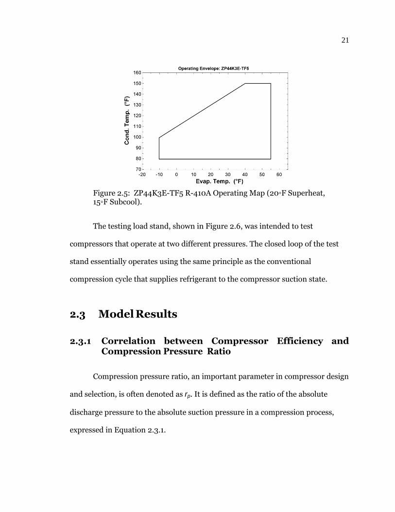
Figure 2.5: ZP44K3E-TF5 R-410A Operating Map (20◦F Superheat, 15◦F Subcool).

The testing load stand, shown in Figure 2.6, was intended to test

compressors that operate at two different pressures. The closed loop of the test

stand essentially operates using the same principle as the conventional

compression cycle that supplies refrigerant to the compressor suction state.

2.3 Model Results

2.3.1 Correlation between Compressor Efficiency and Compression Pressure Ratio

Compression pressure ratio, an important parameter in compressor design

and selection, is often denoted as rp. It is defined as the ratio of the absolute

discharge pressure to the absolute suction pressure in a compression process,

expressed in Equation 2.3.1.

22

Figure 2.6: System Diagram of Copeland Test Setup [3].

23

p2 P

rp ≡ Poutlet

Pinlet

; (2.3.1)

In addition, rp1 represents the first stage compression ratio in a refrigerant-

injected compressor; rp2 represents the second stage compression ratio in a

refrigerant-injected compressor. They are expressed in the following equations

2.3.2 and 2.3.3, where P1 represents inlet pressure; P2 represents outlet pressure.

rp1 ≡ Pinj

P1

; (2.3.2)

r ≡ P2

inj

; (2.3.3)

Compression ratio and volumetric efficiency are closely related terms. It is

necessary to discuss volumetric efficiency first to understand the significance of

compression ratio and its influence on the overall operation of a refrigeration

system. Volumetric efficiency is a ratio of the amount of refrigerant that a

compressor will theoretically compress, to what it actually compresses. In a

reciprocating compressor, the piston reaches top dead center, at the completion

of the discharge stroke, there is a small amount of gas that must expand before

the suction reed opens which starts the suction stroke. This decreases the amount

of gas that is able to enter the cylinder during the suction stroke. If the discharge

pressure increases, the gas left at the top of the cylinder is denser and so it will fill

up more of the cylinder upon re-expansion. The result is a smaller amount of

refrigerant that is able to be compressed, resulting in a decrease in the volumetric

efficiency of the compressor. If the suction pressure changes, the volumetric

efficiency will change as well, and therefore the efficiency of the compressor

24

Figure 2.7: The Correlation of Compressor Efficiency Versus Compression Pressure Ratio.

changes. That’s where the term compression ratio comes in. In this work, that

how the compression pressure ratio affects compressor efficiency is developed in

Figure 2.7 based on the manufacturer’s data. There is also leakage that decreases

the volumetric efficiency.

It is obviously indicated compressor efficiency can be expressed as a

function of the compression ratio across the compressor. A higher discharge

pressure from a dirty condenser or a lower suction pressure caused by low pressure

refrigerant across the evaporator, for example, will greatly reduce system

performance and compressor efficiency.

In order to simulate refrigeration system with injection, a curve fit (shown

in Equation 2.3.4) is made to quantify the relationship between the compressor

efficiency and compression ratio in order to interpolate the compressor

efficiencies at different stages in the compression process.

25

evap

η = −1.46089+2.65662×rp−1.2226×rp2+0.269856×rp

3−0.0293404×rp4+0.001257×rp

5

(2.3.4)

where, r2 = 99.01%.

2.3.2 Correlation between Mass Flow Rate and Evaporating Temperature

If the flow rate of the working fluid in the refrigeration system passing

through the evaporator coil is reduced without changing condenser conditions,

the evaporating pressure and temperature will decrease. Based on the provided

data, the correlation of mass flow rate versus evaporating temperature has been

found and shown in Figure 2.8.

This plot confirms the expectations that the refrigerant mass flow rate

decreases as evaporating temperature decrease. This is mainly due to the

increased specific volume of the refrigerant and reduced volumetric efficiency of

the compressor. Likewise, the compressor efficiency, a curve fit (shown in

Equation 2.3.5) is made to quantify the relationship between mass flow rate and

evaporating temperature.

m = 272.633 + 5.89601 × Tevap + 0.0626164 × T 2 (lbm/hr) (2.3.5)

where, r2 = 99.23%; m is the mass flow rate going through all the conventional

compression cycle; Tevap is the evaporating temperature with the unit of ◦F.

26

Figure 2.8: The Correlation of Mass Flow Rate Versus Evaporating Temperature with 95% Confidence Interval.

2.3.3 Performance Analysis of the Refrigeration Cycle

It is highly anticipated that improvement, if any, due to the injection can

be realized in the system. So how much room does the real system still have to be

improved? The upper performance limit of the refrigeration cycle will be a

reference for people to look up.

The Carnot cycle is a theoretical thermodynamic cycle proposed by Nicolas

Leonard Sadi Carnot in 1824 and expanded upon by others in the 1830’s and

1840’s. The Carnot cycle is a totally reversible cycle that consists of two reversible

isothermal and two isentropic processes. It proves the maximum thermal

efficiency for given temperature limits, and it serves as a standard against which

actual power cycles can be compared.

27

Since it is a reversible cycle, all four processes that comprise the Carnot

cycle can be reversed. Reversing the cycle does also reverse the directions of any

heat and work interactions. The result is a cycle that operates in the counter-

clockwise direction on a T-s diagram. It provides an upper limit on the Coefficient

of Performance of a refrigeration system in creating a temperature difference by

the application of work to the system. Meanwhile it offers the upper performance

limit of the refrigeration cycle for given temperature limits. The coefficients of

performance of Carnot refrigeration system are expressed in terms of

temperature as:

COPrev = (

Tcond

Tevap

−1

− 1)

(T [=] Absolute) (2.3.6)

It is a theoretical system but not an actual thermodynamic cycle, since the

idealizations and simplifications commonly employed in the analysis of power

cycles can be summarized as follows:

1. The cycle does not involve any friction. Therefore, the working fluid

does not experience any pressure drop as it flows in pipes or devices

such as heat exchangers.

2. All expansion and compression processes take place in a quasi-

equilibrium manner.

3. The pipes connecting the various components of a system are well

insulated, and heat transfer through them is negligible.

Comparing the actual system performance the data sheet provides with

that of Carnot refrigeration system, the difference between ideal and actual COPs

28

Figure 2.9: The Correlation of COP Versus Compression Pressure Ratio.

illustrates the potential for improvement. That how much room the real system

still have to be improved have been displayed in the Figure 2.9.

29

Chapter 3

Prediction of the Refrigeration System Performance with Controlled Injection Pressure

3.1 Introduction to Vapor Injection Refrigeration Systems

The vapor injected (VI) scroll compressor makes use of an economizer

within the vapor compression cycle. This cycle offers the advantages of more

cooling capacity and a better COP than with a conventional cycle. Both the

capacity and the COP improvement are proportional to the temperature rise.

Thermodynamically the VI technology offers significant advantages in

applications where temperature rise is high (e.g. water heating, space heating and

refrigeration), and relatively smaller benefits in applications such as residential

air conditioner where efficiency standards are based on tests conducted at very

low temperature rise conditions. This could explain why VI technology is more

widely known and used in residential applications in Europe and Asia, compared

to the U.S. where the residential market is focused almost exclusively on air

conditioning applications.

30

(a) Position of the Injection Ports

in the Scroll Set (b) Internal Tubing Connecting the Injection Inlet with the Scroll Set

Figure 3.1: Position and Tubing Connection for Injection Ports in the Scroll Set [4].

It is usually possible to specify a smaller displacement compressor for a

given cooling load using VI technology. Additionally the cooling provided by the

interstage injection allows the compressor to operate over a similar envelope to a

conventional liquid injected model, and so the vapor-injected scroll can operate

at all the normal low temperature application conditions. Therefore, the vapor

injected scroll compressor has been designed and produced by Copeland. The

scroll injection port location is shown schematically in Figure 3.1 .

31

3.2 Refrigeration System Injected with Isenthalpic Expansion Quality Corresponding to Injection Pressure

To simply investigate the effect of injection on the conventional

refrigeration system, after the refrigerant comes out of condenser, it passes

through an expansion valve used to control the injection pressure, then it is

directly injected to injection ports on the compressor. The refrigeration system

is schematically shown in Figure 3.2.


The thermodynamics of an ideal refrigeration system injected with

controlled injection pressure can be analyzed on a pressure versus enthalpy

diagram as depicted in Figure 3.3. At state 1 in the diagram, the circulating

refrigerant enters the compressor as a 20◦F superheated vapor. From state 1 to

state 9, the vapor is isentropically compressed (i.e., compressed at constant

entropy) to the injection pressure. After which, the vapor mixed with the injected

refrigerant continues to be isentropically compressed to discharge pressure from

state 10 to state 2.

From state 2 to state 3, the vapor travels through part of the condenser

which removes the superheat by cooling the vapor first, then the vapor travels

through the remainder of the condenser, and is further cooled into a 15 ◦F

subcooled liquid. The condensation process always occurs at essentially constant

discharge pressure.

32

Figure 3.2: Refrigeration System Schematic Showing Hardware Components, Flow Connections and State Points.

From states 3 to state 5, the subcooled liquid refrigerant passes through

the expansion valve and undergoes an abrupt decrease of pressure and

temperature to the desired injection pressure. The subcooled liquid refrigerant

becomes a two-phase mixture. Next, the refrigerant splits into two streams: a

portion of the flow passes through another expansion valve from state 6 to state

4, expanding directly to the suction pressure, while the remaining flow is drawn

33

Figure 3.3: P-h Diagram of the Refrigeration System Performance with Controlled Injection Pressure.

off into injection line and directly injected to injection ports of the compressor.

Among state 8, state 9 and state 10, an adiabatic and isobaric

homogeneous mixing process instantaneously occurs in the compressor on the

injection pressure.

From states 4 to state 1, the cold and partially vaporized refrigerant travels

through the coil or tubes in the evaporator where it is totally vaporized by warm

air (from the space being refrigerated) that a fan circulates across the coil or

tubes in the evaporator. The evaporator operates at essentially constant pressure

and boils off all available liquid, thereafter adding 20◦F of superheat to the

refrigerant as a safeguard for the compressor as it cannot compress an

incompressible fluid. The resulting refrigerant vapor returns to the compressor

inlet at state 1 to complete the thermodynamic cycle.

34

It should be noted that the above discussion does not take into account

real world items like frictional pressure drop in the system, internal irreversibility

during the compression process, non-ideal gas behavior or adiabatic and isobaric

homogeneous mixing process.


A model has been developed to predict the refrigeration system

performance with controlled injection pressure over the range of anticipated

operating conditions. The model is intended for use with R-410A as the working

fluid and will be capable of simulating a variety of different compressors. The

model should be easily adaptable to serve as a tool for evaluating the impact of

compressor selection on system performance.

To accomplish this goal, the model uses manufacturer-supplied data to

characterize the compressor performance. Copeland data is typically provided

over a range of condensing and evaporating temperatures with a specified

superheat at the compressor inlet and subcooling at the condenser exit. For a

compressor without injection ports, manufacturers may report the expected

cooling capacity, power consumption, current draw, mass flow rate, EER and

isentropic efficiency of the compressor under each condition. However, the

performance of a compressor designed to operate with economized vapor

injection cannot be characterized as succinctly. Because of the economizer, the

enthalpy of the refrigerant supplied to the evaporator no longer depends on the

degree of subcooling at the condenser exit alone. Therefore, the manufacturer

35

must supply much more information to completely specify the conditions

entering the evaporator and the injection line.

Although the manufacturer may supply information that can be used to

determine the conditions entering the evaporator, additional information is

needed to specify the state of the injected refrigerant. Therefore, providing a

detailed description of the compressor performance is much more complex with

injection.

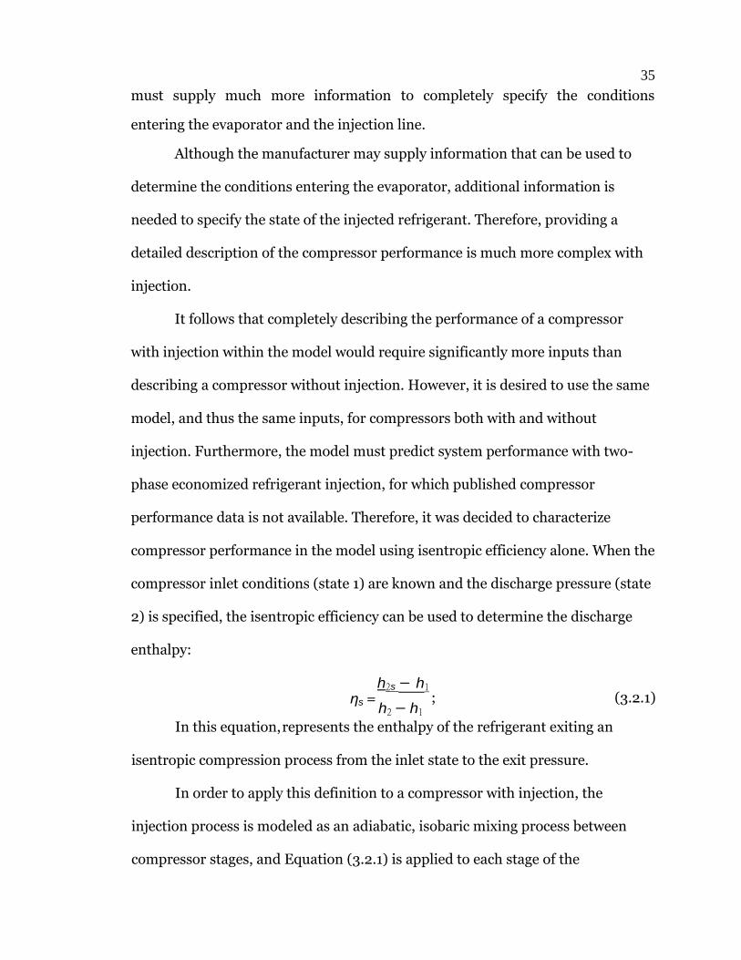
It follows that completely describing the performance of a compressor

with injection within the model would require significantly more inputs than

describing a compressor without injection. However, it is desired to use the same

model, and thus the same inputs, for compressors both with and without

injection. Furthermore, the model must predict system performance with two-

phase economized refrigerant injection, for which published compressor

performance data is not available. Therefore, it was decided to characterize

compressor performance in the model using isentropic efficiency alone. When the

compressor inlet conditions (state 1) are known and the discharge pressure (state

2) is specified, the isentropic efficiency can be used to determine the discharge

enthalpy:

h2s − h1

ηs = h2 − h1

; (3.2.1)

In this equation, represents the enthalpy of the refrigerant exiting an

isentropic compression process from the inlet state to the exit pressure.

In order to apply this definition to a compressor with injection, the

injection process is modeled as an adiabatic, isobaric mixing process between

compressor stages, and Equation (3.2.1) is applied to each stage of the

36

m m

compressor. For example, Equation (3.2.1) can be applied to a compressor with a

single injection port by letting state 9 represent the state of the refrigerant in the

compressor as it reaches the injection pressure. If state inj represents the state of

the injected refrigerant, a mass and energy balance on the adiabatic mixing

process can be used to determine the resulting state of the refrigerant in the

compressor, which will be represented as state 10:

h10 = (1 − Ratiom) × h9 + Ratiom × hinj ; (3.2.2)

For convenience, the injection mass flow rate ratio, Ratiom, is defined as

the ratio of the injection mass flow rate, m inj , to the total mass flow rate existing

the compressor, m total:

Ratio ≡ m inj

total

; (3.2.3)

This ratio is defined relative to the total mass flow rate because it is

assumed that injection will have a negligible impact on the volumetric efficiency

or mass flow rate passing through the compressor. The injection mass flow rate

ratio must be specified by the model user, if injection flow rates are available

from the compressor manufacturer, or can be varied over a range of values to

study the impact on system performance. Following the mixing process, the

refrigerant continues to be compressed and (3.2.1) is used to calculate the

resulting discharge state from the compressor.


model the refrigeration system with injection simplifies the model considerably.

In addition, the following assumptions are proposed:

37

1. Steady-state, steady flow conditions.

2. One-dimensional flow.

3. The compressor can be modeled using an isentropic efficiency.

4. The pressure drop through lines is negligible.

5. Compared to the heat transfer between the condenser and the heat sink,

the heat transfer between the lines and the ambient is negligible.

6. The throttling devices are isenthalpic, with no work or heat transfer.

7. Kinetic and potential energy changes are small relative to changes in

enthalpy and can be disregarded.

8. Any injection processes can be modeled as adiabatic, isobaric mixing

processes.

In addition, the injection pressure ratio, Ratiop, must be specified by the

model user, is denoted as the ratio of the difference between injection pressure

and inlet pressure, Pinj − Pinlet, to the difference between discharge pressure and

suction pressure, Poutlet − Pinlet:

Pinj − Pinlet

Ratiop ≡ P

outlet − Pinlet

; (3.2.4)

Ratiop can be varied over a range of values to conveniently study the

impact on system performance.

The model was implemented using Engineering Equation Solver (Klein,

2009). It requires the user to specify the condensing and evaporating

temperatures, degree of superheat at the compressor inlet and subcooling at the

condenser outlet, compressor power input, mass flow rate and isentropic

efficiency. The compressor manufacturer typically provides all of these

38

parameters on the performance sheet. Making the assumptions mentioned above,

the model then will evaluate the thermodynamic properties at each state, the

mass flow rate through each line in the model, and heat transfer rate in the

condenser.

To clarify the modeling procedure, a flow chart is provided in Figure 3.4.

3.2.3 Sample Calculation and Model Feasibility Analysis

The same condition, where the Copeland compressor can achieve the

highest efficiency in conventional refrigeration system, is picked up for a sample

hand calculation of refrigeration system with injection pressure in the middle of

the range from inlet pressure to outlet pressure. The sample calculation is

intended to make sure there is no errors in the model codes by comparison

between hand calculation results and simulation output. Meanwhile, this hand

calculated process below shows the model procedure literally clear.

1. Conditions:

Tevap = 45◦F , Tcond = 110◦F , m total = 670lbm/hr, ∆TSH = 20◦F , ∆TSC =

15◦F . The compressor efficiency follows the correlations between ηisen and rp

of Equation 2.3.4.

39

Figure 3.4: Flow Chart for The Model of Refrigeration Cycle with Two-Phase Flow Injection.

40

p1 p1 p1 p1

2. Calculations at State 1:

T1 = Tevap + ∆TSH = 45 + 20 = 65◦F

P1 = P ressure(R410A, Tevap = 45◦F, x = 1) = 144.8psia



3. Specify the intermediate pressure ratio of Ratiop as 0.5. Calculations from State

1 to State 9:

Pinj − P1 Pinj − 144.8 Ratiop =

P2 − P1 => 0.5 =

P2 − 144.8


Pinj = Ratiop × (P2 − P1) + P1 = 0.5 × (381.1 − 144.8) + 144.8 = 262.95psia

rp1 = Pinj

P2

262.95 = = 1.816

144.8

η1 = −1.46 + 2.66 × rp1 − 1.22 × r2 + 0.27 × r3

− 0.029 × r4 + 0.00126 × r5

= 0.6534

h9s − h1

h9s − 187.4Btu/lbm η1 =

h9 − h1 => 0.6534 =

h9 − 187.4Btu/lbm

41

m m


P9 = Pinj = 262.95psia

h9s = Enthalpy(R410A, P9 = 262.95psia, s1 = 0.44Btu/lbm ∗ R)

= 195Btu/lbm

h9 = h9s − h1

η1

+ h1 = 195 − 187.4

+ 187.4 = 199.03Btu/lbm 0.6534


5. Specify the injection mass flow rate ratio of Ratiom as 0.1. Calculations for

mixing at the injection port:

Ratio = m inj

total

=> 0.1 = m inj

670

m 2 = m total = 670lbm/hr

m inj = 670 × 0.1 = 67lbm/hr

MassBalance : m 1 + m inj = m 2

m 1 = 670 − 67 = 603lbm/hr

EnergyBalance : m 1 × h9 + m inj × hinj = m 2 × h10

603lbm/hr × 199.03Btu/lbm + 67lbm/hr × hinj = 670lbm/hr × h10


T3 = Tcond − ∆TSC = 110 − 15 = 95◦F

P3 = P2 = 381.1psia


42

r =

p2 p2 p2 p2

7. Calculations at State inj:

hinj = h3 = 110.4Btu/lbm

Pinj = Ratiop × (P2 − P1) + P1 = 0.5 × (381.1 − 144.8) + 144.8 = 262.95psia

Tinj = T emperature(R410A, Pinj = 262.95psia, hinj = 110.4Btu/lbm) = 83.2◦F

xinj = Quality(R410A, Pinj = 262.95psia, hinj = 110.4Btu/lbm) = 0.06


m 1 × h9 + m inj × hinj

603 × 199.03 + 67 × 110.4 h10 = =

m 2

= 190.167Btu/lbm 670

P10 = Pinj = 262.95psia


s10 = Entropy(R410A, P10 = 262.95psia, h10 = 190.167Btu/lbm)

= 0.432Btu/lbm ∗ R

9. Calculations from State 10 to State 2.

P2 p2

inj

381.1 = = 1.449

262.95

η2 = −1.46 + 2.66 × rp2 − 1.22 × r2 + 0.27 × r3

− 0.029 × r4 + 0.00126 × r5

= 0.5214 h2s − h10

h2s − 190.167Btu/lbm η2 =

h2 − h10 => 0.5214 =

h2 − 190.167Btu/lbm

P

43



h2s = Enthalpy(R410A, P2 = 381.1psia, s10 = 0.432Btu/lbm ∗ R)

= 194.9Btu/lbm

h2 = h2s − h10

η2

+ h10 = 194.9 − 190.167

+ 190.167 = 199.24Btu/lbm 0.5214

T2 = T emperature(R410A, P2 = 381.1psia, h2 = 199.24Btu/lbm) = 156◦F


h4 = h3 = 110.4Btu/lbm

P4 = P1 = 144.8psia


44

Table 3.1: State Point Properties of Model with Injection State Pt No.(i) hi( Btu )

lbm Pi(P sia) si( Btu ) lbm∗R Ti(◦F ) xi(−) mi( lbm )

hr

1 187.4 144.8 0.4397 65 SH 603 2 198.4 381.1 0.4377 153.7 SH 670

3 110.4 381.1 0.2841 95 CL 670

4 110.4 144.8 0.2872 44.85 0.2156 603

5 110.4 263 0.2848 83.16 0.0619 670

6 110.4 263 0.2848 83.16 0.0619 603

7 110.4 263 0.2848 83.16 0.0619 67

8 110.4 263 0.2848 83.16 0.0619 67

9 198.7 263 0.4463 134.1 SH 603

10 189.9 263 0.431 103.3 SH 670

12. Overall system

Q evap = m 1 (h1 − h4) = 603lbm/hr (187.4 − 110.4) Btu/lbm = 46431Btu/hr

W comp1 = m 1 (h9 − h1) = 603lbm/hr (199.03 − 187.4) Btu/lbm

= 7012.89Btu/hr = 2055W

W comp2 = m 2 (h2 − h10) = 670lbm/hr (199.24 − 190.12) Btu/lbm

= 6078.91Btu/hr = 1782W

COPR =

W

Q evap

comp1 + W

comp2

46431 = = 3.547

7012.89 + 6078.91

m 1 (h9s − h1) + m 2 (h2s − h10) ηinj =

m 1 (h9 − h1) + m 2 (h2 − h10)

= 603 × (195 − 187.4) + 670 × (194.9 − 190.167)

603 × (199.03 − 187.4) + 670 × (199.24 − 190.167) = 0.5923

The EES program calculation results are summarized in the Table 3.1, for

convenient reference and compared with hand calculation.

45

In this section, the feasibility of the model will be analyzed by proving that

the coefficient of performance of the injection system equals to that of the

conventional system when the injection pressure ratio and mass fraction go

towards 1 and 0 respectively, Ratiop→1 and Ratiom→0, or when both the injection

pressure ratio and mass fraction go towards 0, Ratiop→0 and Ratiom→0.

The COP of the conventional system on the same condition has been found

in Chapter 2, which is 4.677, while the COP of the refrigeration system with

injection equals to 4.657 when specifying the values of Ratiop and Ratiom as 0.9999

and 0.0001 in the EES program, or 4.655 when specifying the values of both

Ratiop and Ratiom as 0.0001 in the EES program.

As such, the feasibility of the model of refrigeration system with injection

has been proven reasonably.

3.2.4 Pre-Simulation Work

In order to investigate the two-phase fluid injection impact on the system,

a well-planned approach is necessary to guide the simulation of the refrigeration

cycle system in a scroll compressor with two-phase fluid injection. All the

refrigeration system performance points are investigated under different

intermediate pressure between input pressure and output pressure, different

injection mass flow rate and different injection quality. A parametric

investigation Table 3.2 will provide a clear vision of the whole investigation.

There are total 57 operating conditions in the manufacturer’s data sheet. It

will be a repetitive and time-consuming process to run all the cases. It is very

46

Table 3.2: Parametric Investigation Table Intermediate Pressure Ratio Mass Fraction Injection Quality Output

Ratiop = Pinj−P1

P2 −P1

Ratiom = minj

m

x COP, ηinj

0.1 0.01 to 0.99 0 to 1

0.3 0.01 to 0.99 0 to 1

0.5 0.01 to 0.99 0 to 1

0.7 0.01 to 0.99 0 to 1

0.9 0.01 to 0.99 0 to 1

necessary to select the desired conditions to focus the analysis. Because

evaporating temperature is more relevant to cooling capacity, which is the

concern in refrigeration system, the minimum and maximum compressor

efficiency cases for each certain evaporating temperature are classified into

Group A and Group B, respectively. The classification result is shown in Figure

3.5.

3.3 Model Results

3.3.1 Case Study of Minimum Compressor Efficiency Group

Group A represents the cases where compressor efficiencies reach the

minimum values on each certain evaporating temperature in the feasible range. It

includes two extreme cases:

1. A1: maximum compression ratio case including minimum evaporating

temperature and minimum compressor efficiency;

2. A6: maximum condensing temperature case.

Three cases from Group A and one case from Group B were chosen to run

the simulation, which are A1, A4, A6 and B1. Although B1 is maximum

47

Figure 3.5: Demonstration of Group Setup.

48

Figure 3.6: Location of the Potential Performance Improvement Group.

compressor efficiency case under -10◦F evaporating temperature, it still has a

very low compressor efficiency compared with the other cases. In sum, all the

four representative cases have a common feature that they have very low

compressor efficiency and very poor system performance in the conventional

refrigeration system. They represent the blocks marked in the simplified data

sheet of Figure 3.6 by highlighting in red with the name of potential performance

improvement group.

After the simulation runs, the performance of the system at the four

desired conditions is plotted in Figure 3.7. Additionally, the maximum COP that

it can be achieved at each condition is also shown in the plot with the

corresponding mass fraction and injection pressure ratio. In addition, the

49

Figure 3.7: System Performance of Potential Performance Improvement Cases.

50

locations on the data sheet for each case are evidently marked in a simplified data

sheet on the upper right corner of each plot.

It is obvious that potential performance improvement cases have very low

compressor efficiency. Under the conditions of these cases, the refrigeration

system with injection can achieve better performance than the conventional

system in a wide range of injection pressure ratio if injecting refrigerant less than

70% mass fraction in this group. No additional benefit is attained in the high

potential COP improvement group if injecting refrigerant more than 90% mass

fraction.

On the operating condition of case A1, a maximum COP of 2.229 occurs

when injecting refrigerant at 22.95% of mass fraction and holding the injection

pressure ratio at 0.2818. The system performance is improved 55% over the

conventional refrigeration system with the COP of 1.44 on the same operating

condition. Similarly, for case A4, case A6 and case B1, each system performance

is improved 29%, 19% and 23% by injection, respectively over their conventional

refrigeration system performance.

Only when conventional refrigeration system has very low compressor

efficiency and very poor system performance, can the cycle obtain benefit from

injecting refrigerant into the compressor. The potential COP improvement in this

group rises with the evaporating temperature deceasing and condensing

temperature increasing. The case A1 has the best potential COP improvement

over all the other cases with 55% performance improvement.

3.3.2 Case Study of Maximum Compressor Efficiency Group

51

Figure 3.8: Location of the None Potential Performance Improvement Group.

Group B represents the cases where compressor efficiencies reach the

maximum values on an each certain evaporating temperature in the feasible

range. It includes two extreme cases:

B1: minimum evaporating temperature and condensing temperature

case;

B7: maximum compressor efficiency case.

Four cases from Group B were chosen to run the simulation, which are B3,

B4, B7 and B9. In sum, all the four representative cases have a common feature

that they have high compressor efficiency and very excellent system performance

in the conventional refrigeration system. They represent the blocks marked in the

simplified data sheet of Figure 3.8 by highlighting in red with the name of none

52

Figure 3.9: System Performance of the None Potential Performance Improvement Cases.

53

potential Performance improvement group.

After the simulation runs, the performances of the system on the four

desired conditions is plotted in Figure 3.9. The locations on the data sheet for

each case are evidently marked in a simplified data sheet on the upper right

corner of each plot.

It is obvious that no potential performance improvement cases have very

high compressor efficiency. Under the conditions of these cases, the refrigeration

system with injection definitely got worse performance than conventional system

in all the range of injection pressure ratio no matter how much refrigerant is

injected. Injection would not get any benefits in this group.

When a conventional refrigeration system has a high compressor

efficiency and good system performance, the cycle cannot obtain benefits from

injecting refrigerant to compressor. However, the plots indicate that refrigeration

system with injection trends to be close to conventional refrigeration system at

around 0.3 of injection pressure ratio with the evaporating temperature

deceasing and condensing temperature increasing.

3.3.3 Trend Prediction of Refrigeration System Performance with Injection

Two cases from Group A, one case from Group B and an additional case

were chosen to run the simulation, which are A4, A9, B7 and X. Case A9 belongs

to the minimum compressor efficiency group, representing the maximum

evaporating temperature and minimum condensing temperature case. The

additional case X is used to represent the case between the potential performance

54

Figure 3.10: Location of the Cross Cases Group.

Figure 3.11: Trend Prediction of Refrigeration System Performance with Injection.

55

Figure 3.12: System Performance of Cross Cases.

56

improvement group and none potential performance improvement group.

In sum, all the four representative cases gather to form into a new group

named with cross group. They represent the blocks marked in the simplified data

sheet of Figure 3.10 by highlighting in red.

After the simulation runs, the performances of the system on the four

desired conditions are plotted in Figure 3.12. The locations on the data sheet for

each case are evidently marked in a simplified data sheet on the upper right

corner of each plot.

These plots are indicated that the COP of the refrigeration system with

injection undergoes a gradual process of rising with the evaporating temperature

deceasing and condensing temperature increasing. The changing process is

shown in Figure 3.11.

57

Chapter 4

Prediction of the Refrigeration System Performance with Controlled Injection Fluid Quality

After the investigation of a refrigeration system injected with controlled

injection pressure on the conditions of the potential performance improvement

group, a maximum COP of 2.229 occurs for the case A1 when injecting refrigerant

at 22.95% of mass fraction and holding the injection pressure ratio at 0.2818. The

system performance is improved 55% over the conventional refrigeration system

with the COP of 1.44 for the same operating conditions. Similarly, for case A4,

case A6 and case B1, each system performance is improved by injection 29%, 19%

and 23%, respectively over their conventional refrigeration system performance.

(See Figure 3.7).

However, system performance in previous model has been improved by

injecting two-phase refrigerant fluid, which may cause compressor failures.

Essentially, slugging is the result of trying to compress liquid refrigerant in the

compressor. HVAC&R technicians have been aware of compressor failures caused

by slugging for many years. It used to be a much greater problem, and more

emphasis was put on it. Today many compressor failures are still attributed to

slugging.

A further investigation on the potential performance improvement group is

58

conducted based on a refrigeration system injected with controlled injection fluid

quality. This model is intend to investigate the optimum refrigeration system

performance with injection, taking into account the slugging problem. The

slugging problem is addressed by maintaining a minimum degree of superheat in

the compressor.

4.1 Refrigeration System Injected with Controlled Injection Quality

In order to keep compressors from slugging, it is necessary to maintain the

refrigerant mixture temperature within the scroll compressor at least 20◦F above

the saturation temperature at the injection pressure, which is widely accepted by

HVAC&R manufacturers.

To further investigate the effect of injection on the conventional

refrigeration system with this constraint of 20◦F, after the refrigerant comes out

of condenser, it passes through an expansion valve used to control the injection

pressure, then it is heated to the desired quality by an intermediate heat

exchanger before injected to injection ports on the compressor. The refrigeration

system is schematically shown in Figure 4.1.


The thermodynamics of a refrigeration system injected with controlled

injection fluid quality can be analyzed on a pressure versus enthalpy diagram as

ideally depicted in Figure 4.2. At state 1 in the diagram, the circulating refrigerant

59

Figure 4.1: Refrigeration System Schematic Showing Hardware Components, Flow Connections and State Points.

60

Figure 4.2: P-h Diagram of the Refrigeration System Performance with Controlled Injection Quality.

enters the compressor as a 20◦F superheated vapor. From state 1 to state 9, the

vapor is isentropically compressed (i.e., compressed at constant entropy) to the

injection pressure. After which, the vapor mixed with the injected refrigerant

continues to be isentropically compressed to the discharge pressure from state 10

to state 2.

From state 2 to state 3, the vapor travels through a part of the condenser

which removes the superheat by cooling the vapor travels through the remainder

of the condenser and is condensed to a 15◦F subcooled liquid. The

condensation process occurs at essentially constant pressure.

From state 3 to state 5, the subcooled liquid refrigerant passes through the

expansion valve and undergoes an abrupt decrease of pressure and temperature

to the desired injection pressure. The subcooled liquid refrigerant becomes two-

phase mixture. Next, the refrigerant splits into two streams: a portion of the flow

61

passes through another expansion valve from state 6 to state 4, expanding

directly to the suction pressure, while the remaining refrigeration flow is drawn

off into an injection line and heated in an intermediate heat exchanger (IHX)

from state 7 to state 8 to control the injection fluid quality prior to injection into

the ports of the compressor.

Among state 8, state 9 and state 10, an adiabatic and isobaric

homogeneous mixing process occurs in the compressor at the injection pressure.

From state 4 to state 1, the cold and partially vaporized (i.e. low quality)

refrigerant travels through the evaporator coil or tubes, where it is totally

vaporized by warm air (from the space being refrigerated). A fan circulates air

across the coil or tubes in the evaporator. The evaporator operates at essentially

constant pressure and boils off all available liquid thereafter adding 20◦F of

superheat to the refrigerant as a safeguard for the compressor, as it cannot

tolerate any incompressible fluid. The resulting refrigerant vapor returns to the

compressor inlet at state 1 to complete the thermodynamic cycle.

It should be noted that the above discussion is based on some assumptions

which does not take into account real world items like frictional pressure drop in

the system, internal irreversibility during the compression process, non-ideal gas

behavior or adiabatic and isobaric homogeneous mixing process.


A modification has been made to the model of the refrigeration system

injected with controlled injection pressure. An intermediate heat exchanger (IHX)

62

is installed into the injection line. The injected refrigerant fluid quality can be

controlled by heating the injection line. The updated simulation model has the

function to predict refrigeration cycle performance over the range of anticipated

operating conditions, using R-410A as the working fluid and will be capable of

testing a variety of different compressors with a safeguard to keep them from

slugging.

The model uses manufacturer-supplied data from Copeland to

characterize the compressor performance. This data is typically provided over a

range of condensing and evaporating temperatures with a specified superheat at

the compressor inlet and subcooling at the condenser exit. For a compressor

without injection ports, manufacturers report the expected cooling capacity,

power consumption, current draw, mass flow rate, EER and isentropic efficiency

of the compressor under each operating condition. However, the performance of

a compressor designed to operate with economized vapor injection cannot be

characterized as succinctly. Because of the economizer, the enthalpy of the

refrigerant supplied to the evaporator no longer depends on the degree of

subcooling at the condenser exit alone. Therefore, the manufacturer must supply

much more information to completely specify the conditions entering the

evaporator and the injection line.

Although the manufacturer may supply information that can be used to

determine the conditions entering the evaporator, additional information is

needed to specify the state of the injected refrigerant. Therefore, providing a

detailed description of the compressor performance is much more complex with

injection.

63

It follows that completely describing the performance of a compressor

with injection within the model would require significantly more inputs than

describing a compressor without injection. However, it is desired to use the same

model, and thus the same inputs, for compressors both with and without

injection. Furthermore, the model must predict system performance with two-

phase economized refrigerant injection, for which published compressor

performance data is not available. Therefore, it was decided to characterize

compressor performance in the model using isentropic efficiency alone, which

was explained in the section of model of the system in Chapter 3.

In order to control the injection fluid quality, an internal heat exchanger is

employed in the injection line of the model. When the IHX inlet (state 7) and the

heat transferred into injection line is specified, the injection fluid quality can be

determined (state 8) in the following equations:

Q IHX = Ratiom × m total (h8 − h7) ; (4.1.1)

x8 = Quality (R410A, P8, h8) ; (4.1.2)

In this equation, x8 represents the quality of the refrigerant exiting the

IHX, which also means the injection fluid quality. (See Figure 4.1).


model the refrigeration system with injection simplifies the model considerably.

In addition, the same assumptions as the model in Chapter 3 are applied to the

model of the refrigeration system with controlled injection fluid quality.

The model was implemented using Engineering Equation Solver (Klein,

2009). It requires the user to specify the condensing and evaporating

64

temperatures, degree of superheat at the compressor inlet and subcooling at the

condenser outlet, compressor power input, mass flow rate and isentropic

efficiency. The compressor manufacturer typically provides all of these

parameters on the published performance sheet. Making the assumptions

mentioned above, the model will then calculate the thermodynamic properties at

each state, the mass flow rate through each line in the model, and heat transfer

rate in the condenser.

The flow chart has been provided in Figure 3.4 of Chapter 3, which

represents the modeling procedure for the refrigeration system with controlled

injection fluid quality.

4.2 Model Results

4.2.1 Continuous Case Study of Minimum Compressor Efficiency Group

Temperature Profile at Injection Port in the Compressor

The same as the inlet situation that refrigerant enters the compressor as a

20◦F superheated vapor, it is also necessary to maintain the refrigerant mixture

temperature within the scroll compressor at least 20◦F above the saturation

temperature at the injection pressure, to keep it from slugging.

The way the injection fluid quality being controlled is to simply use an

intermediate heat exchanger to heat the injection fluid. The desired injection

fluid quality can be achieved by heating to the fluid. It is easy to determine the

relationship between refrigeration system performances with injection fluid

65

quality.

The potential system performance improvement group in the previous

model has been improved by injecting two-phase refrigerant fluid, but risks

putting the compressor into a slugging situation. The temperature at the injection

port in the compressor is straightforward to determine if the mixed refrigerant in

the compressor stays in the superheated region. The temperature profiles at the

injection port will display a clear vision of how the mixed refrigerant in the

compressor changes with the addition of heat and where the constraint appears

in the performance profiles.

After the runs of program on the same conditions as the four cases’ in the

potential performance improvement group, the temperature profiles at the

injection port by different amounts of heat transfer are shown in the Figure 4.3

below. The constraint has been marked on the temperature profiles as a dashed

line.

The plots indicate that a certain heat should be transferred into the

injected refrigerant fluid to keep it at a 20◦F superheated status. More heat

should be transferred into if the injected refrigerant fluid stays in a low

compression ratio; otherwise, less heat is required even no heat if the fluid stays

in a high compression ratio. Therefore, there must be a value of the heat transfer

that not only satisfies the constraint but also corresponds to an optimum system

performance.

66

Performance of the Refrigeration System Performance with Controlled Injection Fluid Quality

The performance of the refrigeration system injected with controlled

injection fluid quality is investigated using the new model based on the four cases

of A1, A4, A6 and B1 in the potential performance improvement group. The result

is displayed in the plot shown in Figure 4.4.

The blue lines in the plots represent the optimum performance of the

refrigeration system with controlled injection pressure over different

compression ratios. It is illustrated that the system performance is degraded by

heating the injected refrigerant fluid. So it would not be necessary to transfer too

much heat into the injection line. The dashed line in the plot represent the system

performance of the refrigeration system on the constraint that keeping

compressor from slugging.

The maximum COP for the refrigeration system injected with controlled

injection fluid quality will appear at the peak of the dashed line. For the case A1,

the maximum COP of 2.063 occurs when injecting refrigerant at 22.95% of mass

fraction, holding the injection pressure ratio at 0.3232 and transferring the heat

in at 1862 Btu/hr. The system performance is improved 43% over the

conventional refrigeration system with the COP of 1.44 for the same operating

condition. Nearly 12% performance improvement is sacrificed to keep the

compressor from slugging.

Similarly, for case A4, case A6 and case B1, each system performance is

improved 19%, 11% and 14% by injection, respectively over their conventional

refrigeration system performance, as well as nearly 10%, 8% and 9% performance

67

Figure 4.3: Temperature Profiles at Injection Port by Different Amounts of Heat transfer.

68

Figure 4.4: Cycle Performance Improvement with Controlled Injection Quality

69

improvement have been sacrificed respectively, to keep the compressor form

slugging.

Injection Fluid Quality

In addition, injection fluid quality for each of the cases is shown on the

plot of Figure 4.5. The plot illustrates how the injection fluid quality changes with

heat transfer.

According to the condition where the refrigeration system with injection

achieve the best performance, the injection fluid quality values for the four cases

of A1, A4, A6 and B1 can be found on the plots, being 0.6123, 0.64, 0.6225 and

0.6138, respectively. The optimum refrigeration system performance with

injection occurs when the injection quality ranges from 0.61 to 0.64.

4.2.2 Sensitivity Analysis of Coefficient of Performance of the Refrigeration System with Two-Phase Fluid Injection

The usefulness of any mathematical model depends in part on the

accuracy and reliability of its input. Yet, because all models are imperfect

abstractions of reality, and because precise input data are rarely if ever available,

all output values are subject to inaccuracies. As such, uncertainty and sensitivity

analysis is necessary to understand the mathematical model and behavior of the

system.

70

Figure 4.5: Injection Quality Profile.

71

Table 4.1: Sensitivity Analysis of Optimal Results of Case A1 (Tevap = −10◦F|Tcond = 100◦F )

Variable±Uncertainty Partial Derivative % of Uncertainty

COPR = 2.063 ± 0.027

Ratiom = 0.2295 ± 10% ∂COPR/∂Ratiom = −0.5692 23.41%

Ratiop = 0.3232 ± 10% ∂COPR/∂Ratiop = −0.3975 22.65%

xinj = 0.6123 ± 10% ∂COPR/∂xinj = −0.3238 53.94%

Table 4.2: Sensitivity Analysis of Optimal Results of Case A4 (Tevap = 20◦F|Tcond = 130◦F )


COPR = 2.01 ± 0.02799



xinj = 0.64 ± 10% ∂COPR/∂xinj = −0.3137 51.46%

Table 4.3: Sensitivity Analysis of Optimal Results of Case A6 (Tevap = 40◦F|Tcond = 150◦F )


COPR = 1.908 ± 0.02614



xinj = 0.6225 ± 10% ∂COPR/∂xinj = −0.2833 45.52%

Table 4.4: Sensitivity Analysis of Optimal Results of Case B1 (Tevap = −10◦F|Tcond = 80◦F )


COPR = 2.701 ± 0.02885



xinj = 0.6138 ± 10% ∂COPR/∂xinj = −0.3659 60.60%

72

Uncertainty analysis, also called sensitivity analysis, is the study of how

the uncertainty in the output of a mathematical model or system can be

apportioned to different sources of uncertainty in its inputs. Uncertainty analysis

has a greater focus on uncertainty quantification and propagation of uncertainty.

For the model of the refrigeration system with injection, the system

performance is assessed by COP, which is the output of the mathematical model.

The system performance can be apportioned to three sources of uncertainty in its

inputs of injection mass fraction, injection pressure ratio and injection fluid

quality. (i.e., the independent variables in the model).

Therefore, uncertainty analysis of coefficient of performance on

refrigeration system with injection is conducted through EES program on the

four cases in the potential performance improvement group. The results are

shown in the Tables of 4.1, 4.2, 4.3 and 4.4, respectively:

In sum, the injection fluid quality has a significant effect on the

refrigeration system with injection. The injection mass fraction has a much less

effect than injection fluid quality but a little more effect than injection pressure

ratio on the system performance.

Note that the independent variables are varied by 10 percent, yet the

variation of COP is only approximately 1%.

73

Chapter 5

Summary and Conclusions

5.1 Summary

There are many opportunities to improve the performance of vapor

compression equipment through the use of advanced compression techniques

such as multi-stage compression or compression with refrigerant injection. The

completed work presented in this paper represents significant progress towards

understanding the potential benefits and limits of a refrigeration system modified

to use these compression techniques with two-phase refrigerant fluid injection.

A model of the conventional compression cycle was developed to serve as a

basis for investigating cycles with two-phase injection. In order to analyze the

model practically, the Copeland scroll compressor system data sheet provided a

range of anticipated operating conditions with a specified superheat at the

compressor inlet and subcooling at the condenser exit, the working fluid R-410a,

the expected cooling capacity, power consumption, current draw, mass flow rate,

EER and isentropic compressor efficiency under selected operating conditions.

Based on all above, the basic cycle performance analysis was theoretically

simulated using EES software to conclude the correlation between the

compressor efficiency and the compression pressure ratio as well as the

correlation between mass flow rate and evaporating temperature.

The development of the basic cycle model with two-phase refrigerant fluid

74

injection provided a means for investigating the performance of the refrigeration

system with two-phase refrigerant fluid injection, and confirmed the ability of

this modifications to improve cycle performance.

The developed basic cycle model with two-phase refrigerant fluid injection

was numerically analyzed, considering that the refrigerant exiting the condenser

passes through an expansion valve used to control the injection pressure, then it

is directly injected into the injection ports on the compressor. The analysis

indicated the operating conditions on the data sheet where the injection has the

best potential to improve the system performance and also investigated the

conditions where the optimum system performance occurs.

To further investigate the effect of injection on the conventional

compression cycle with the constraint of maintaining the refrigerant mixture

within the compressor at least 20◦F above the saturation temperature, it is

considered that the refrigerant is heated to the desired quality before injected

to injection ports on the compressor. Similarly, the developed basic cycle model

with two-phase refrigerant fluid injection was numerically analyzed again to find

the conditions where the optimum system performance occurs. Additionally, an

uncertainty analysis of coefficient of performance was conducted on the

refrigeration system with two-phase fluid injection.

75

5.2 Conclusions

The optimum benefits of two-phase injection are most pronounced for

cycles operating across a large temperature difference , with up to a 55%

improvement in COP at an evaporating temperature of -10 ◦F and a condensing

temperature of 100 ◦F, by holding the injection pressure ratio at 0.2818 and

injection mass fraction at 0.2295. Considering the constraint of maintaining the

refrigerant mixture temperature within the compressor at least 20◦F above the

saturation temperature at the injection pressure, the optimum benefits of the

two-phase injection are still significant for cycles operating across the same large

temperature difference, with up to a 43% improvement in COP by increasing the

injection mass pressure ratio to 0.3232 and holding the injection mass fraction at

0.2295, as well as the injection quality at 0.6123.

By sensitivity analysis on the simulation of the refrigeration system with

two-phase fluid injection, the injection fluid quality has a significant effect on the

refrigeration system COP. The injection mass fraction has a much less effect than

injection fluid quality but a little more pronounced than injection pressure ratio

on the system performance. For the operating condition where the refrigeration

system with two-phase fluid injection achieve the best potential COP

improvement, varying the independent variables (injection mass fraction,

injection pressure ratio and injection fluid quality) by ±10%, the uncertainty of

the injection mass fraction, injection pressure ratio and injection fluid quality are

23.41%, 22.65% and 53.94%, respectively, yet the variation of COP is only

approximately 1.3%.

76

Bibliography

[1] “Refrigeration,” URL: https://en.wikipedia.org/wiki/Refrigeration.

[2] “Online product infomation,” URL:

https://opi.emersonclimate.com/was.extension.opi.web/OPIServlet.

[3] R. J. G. Gordan J. Gerber and J. H. Karian, “Performance test code on

compressors and exhausters,” The American Society of Mechanical

Engineers, 1998.

[4] W.Bianchi and E. Winandy, “Performance improvements in

commercial refrigeration with vapour injected scroll compressors,”

Emerson Climate Technologies.

[5] “Residential energy consumption survey, 2005,” URL:

http://www.eia.doe.gov/emeu/recs/.

[6] H. H. Cho and Y. Kim, “Experimental study on an inverter-driven scroll

compressor with an injection system,” International Compressor

Engineering Conference, p. 1463, 2000.

[7] Y. M. F. Liu, H. Huang and R. Zhuang, “An experimental study on the

heat pump water heater system with refrigerant injection,” In:

Proceedings of International Refrigeration and Air Conditioning

Conference at Purdue, pp. 2211–2216, 2008.

[8] Y. H. Xudong Wang and R. Radermacher, “Performance investigation of

http://www.eia.doe.gov/emeu/recs/

77

refrigerant vapor-injection technique for residential heat pump

systems,” International Refrigeration and Air Conditioning Conference

at Purdue, 2008.

[9] Y. H. Xudong Wang and R. Radermacher, “Two-stage heat pump

system with vapor-injected scroll compressor using r410a as a

refrigerant,” International Journal of Refrigeration, vol. 32, pp. 1442–

2451, 2009.

[10] K. S. H. K. H. Yamazaki, T. Itoh and M. Kawada, “High performance

scroll compressor with liquid refrigerant injection,” International

Compressor Engineering Conference, p. 1596, 2002.

[11] V. A. Jon Winkler, Xudong Wang and R. Radermacher, “Simulation and

validation of a two-stage flash tank cycle using r410a as a refrigerant,”

International Refrigeration and Air Conditioning Conference at Purdue,

2008.

[12] J. G. Jain Siddharth and B. Clark, “Vapor injection in scroll

compressors,”International Compressor Engineering Conference at

Purdue, 2004.

[13] Z. Liu and W. Soedel, “An investigation of compressor slugging

problems,” International Compressor Engineering conference at

Purdue, pp. 433–440, 1994.

[14] Z. Liu and W. Soedel, “A mathematical model for simulating liquid and

vapor two-phase compression processes and investigating slugging

problems in compressors,” HVACR Research, vol. 1, no. 2, pp. 90–109,

1995.

[15] J. E. B. Margaret M. Mathison and E. A. Groll, “Approaching the

performance limit for economized cycles using simplified cycles,”

International Journal of Refrigeration, vol. 45, pp. 67–72, 2014.

78

[16] J. E. B. Margaret M. Mathison and E. A. Groll, “Performance limit for

economized cycle with continuous refrigerant injection,” International

Journal of Refrigeration, vol. 34, no. 1, pp. 234–242, 2011.

[17] R. Rajendran and A. Nicholson, “Air-conditioning, heating, and

refrigeration institute (ahri) low-gwp alternative refrigerants evaluation

program (low-gwp arep),” Emerson Climate Technologies, Inc.,2013

79

APPENDIX I.

EES CODES FOR CONVENTIONAL VAPOR COMPRESSION REFRIGERATION C Y C L E

80

81

82

APPENDIX II.

EES CODES FOR REFRIGERATION SYSTEM WITH TWO-PHASE FLUID INJECTION

83

84

85

86

Documents

Modeling and Investigation of Refrigeration System