Embed Size (px)
Citation preview
1016 K. Y. YOU, Z. ABBAS, C.Y. LEE, ET AL., MODELING AND MEASURING DIELECTRIC CONSTANTS …
Modeling and Measuring Dielectric Constants for Very Thin Materials Using a Coaxial Probe
K. Y. YOU1, Z. ABBAS2, C. Y. LEE3, M. F. A. MALEK4, K. Y. LEE5, E. M. CHENG6
1 Dept. of Radio Communication Engineering, Faculty of Electrical Engineering, Universiti Teknologi Malaysia, 81310 UTM Skudai, Malaysia
2 Dept. of Physics, Faculty of Science, Universiti Putra Malaysia, 43400 UPM Serdang, Malaysia 3Faculty of Bioscience & Medical Engineering, Universiti Teknologi Malaysia
4 School of Electrical Systems Engineering, Universiti Malaysia Perlis, Kuala Perlis, Perlis, Malaysia 5Dept. of Electrical and Electronic Engineering, Faculty of Engineering and Science,
Universiti Tunku Abdul Rahman, 46200 Selangor, Malaysia 6School of Mechatronic Engineering, Universiti Malaysia Perlis, 02600 Arau, Perlis, Malaysia
[email protected], [email protected], [email protected], [email protected], [email protected], [email protected]
Abstract. This paper is focused on the non-destructive measurement of the dielectric constants (relative permit-tivities) of thin dielectric material (0.1–0.5 mm) using an open-ended coaxial probe with an outer diameter of 4.1 mm. Normalized de-embedding and network error calibration procedures were applied to the coaxial probe. The measured reflection coefficients for the thin samples were taken with a vector network analyzer up to 7 GHz, and the calibrated reflection coefficients were converted to relative dielectric constants using an empirical reflection-coefficient model. The empirical model was created using the regression method and expressed as a polynomial model, and the coefficients of the model were obtained by fitting the data using the Finite Element Method (FEM).
Keywords Relative effective permittivity, one-port calibration, measured reflection coefficient, open-ended coaxial probe, thin dielectric substrate.
1. Introduction Recently, there has been an increase of interest in the
determination of the dielectric properties of thin samples in the microwave frequency range, such as conducting di-electric tests of thin-film materials in the fields of physics and engineering [1], as well as for the characterization of biological samples. In practice, the prime considerations in measuring the dielectric properties of the samples are the minimum thickness required to assume an infinite medium, the size of the sensor, limitations of the operational fre-quency, and the accuracy of the measurements.
Various two-port waveguide methods have been pro-posed for measuring the dielectric properties of thin materi-
als, but some of those methods require specific dimensions for the thin-layer sample so that it will fit inside the given size of the waveguide [2], [3]. When using this method for thin samples, i.e., the thickness of the sample must be less than λ/4, it has been conventional practice to measure the reflection coefficient, Γ, and the transmission coefficient, T, by using the Nicholson-Ross-Weir (NRW) method [3], [4] or improved NRW routines [1], [5], [6]. Then, these measurements are converted to relative permittivity, εr, and relative permeability, μr, respectively. For non-destructive modification of the two-port measurement, for which the thin sample is placed between two aperture waveguides, the conversion process to acquire εr and μr requires a robust numerical analysis [7], [8].
Generally, an open-ended coaxial probe method is the simplest, broadband, non-destructive way to measure the dielectric properties of a material. This method is a one-port measurement that only measures the reflection coeffi-cient, Γ, for the sample, and it is suitable for measuring the relative permittivity, εr, of the dielectric material (non-magnetic material, μr = 1). However, a sample that has significant thickness is required for regular measurement in which an open-ended coaxial probe is used. This is re-quired because the scattering of the wave from the probe’s aperture would penetrate a very thin sample and impinge on the other layer-interface media. Normally, the sample is considered to be infinitely thick if its thickness, h, is as large as or larger than the diameter of the outer conductor, 2b, for the coaxial probe (i.e., condition: h ≥ 2b) [9]. Of course, a smaller and very slim coaxial probe could meet these needs for a thin-gauge material. But the uncertainty associated with fabricating a very small, slim, steel coaxial probe is significant, as is the uncertainty associated with the measurement of a thin sample (< 0.5 mm). In addition, the smallest commercial, coaxial waveguide available only has a 2b value of approximately 0.5 mm. Thus, this sensi-tive measurement could only be performed at very high
RADIOENGINEERING, VOL. 23, NO. 4, DECEMBER 2014 1017
operational frequency (> 10 GHz) for a low-loss sample. In previous studies, the dielectric constant of a thin sample backed by metal plate was predicted from the measured reflection coefficient, Γ, via a quasi-static admittance model without involving the higher- order modes, TM0n [10]. The reason is that an infinite higher-order series term of the quasi-static integration must be solved, which makes the calculations more complex. However, it is known that the higher order modes, TM0n, occur due to the disconti-nuity-fringing effect at the aperture of the probe, which has a significant effect on the measured reflection coefficient, Γ, of very thin material (< 0.5 mm) backed by a metal plate.
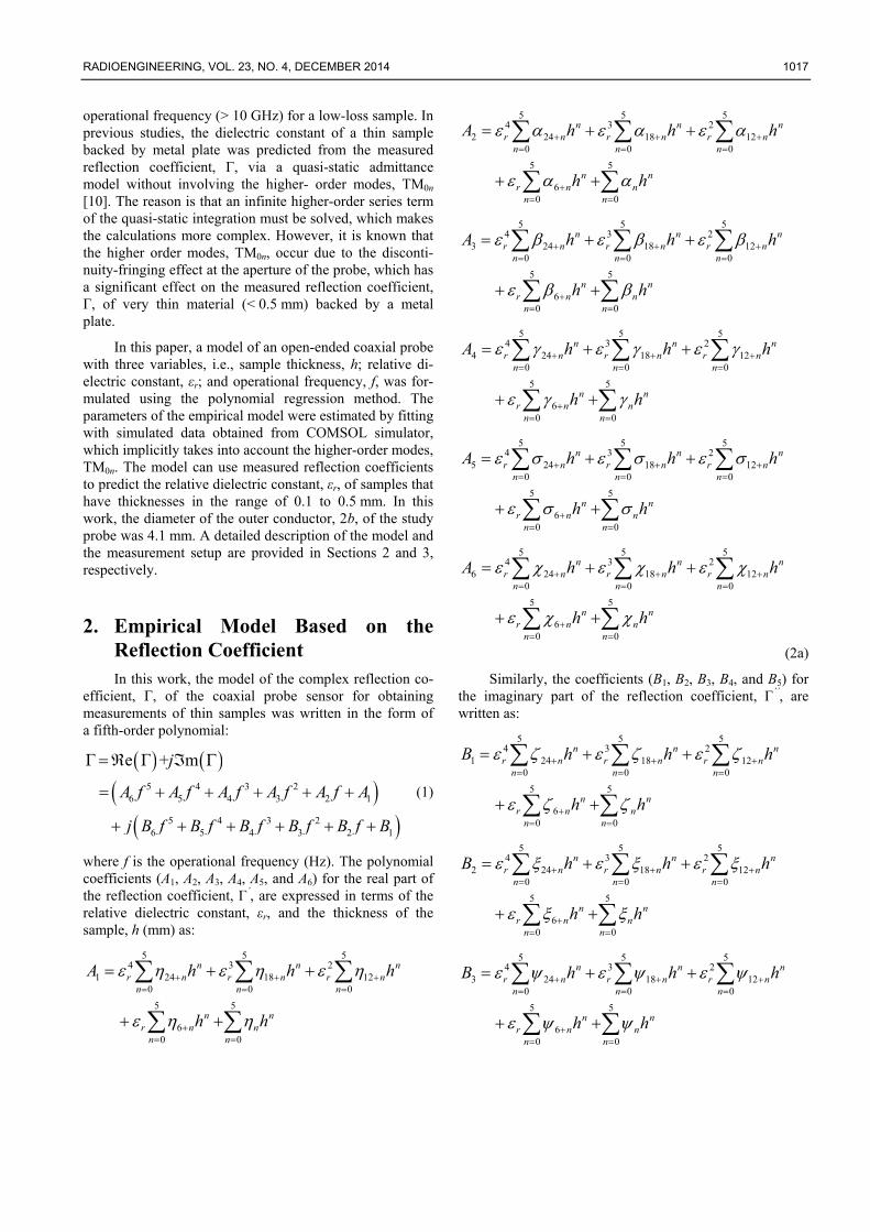
In this paper, a model of an open-ended coaxial probe with three variables, i.e., sample thickness, h; relative di-electric constant, εr; and operational frequency, f, was for-mulated using the polynomial regression method. The parameters of the empirical model were estimated by fitting with simulated data obtained from COMSOL simulator, which implicitly takes into account the higher-order modes, TM0n. The model can use measured reflection coefficients to predict the relative dielectric constant, εr, of samples that have thicknesses in the range of 0.1 to 0.5 mm. In this work, the diameter of the outer conductor, 2b, of the study probe was 4.1 mm. A detailed description of the model and the measurement setup are provided in Sections 2 and 3, respectively.
2. Empirical Model Based on the Reflection Coefficient In this work, the model of the complex reflection co-
efficient, Γ, of the coaxial probe sensor for obtaining measurements of thin samples was written in the form of a fifth-order polynomial:
5 4 3 26 5 4 3 2 1
5 4 3 26 5 4 3 2 1
Γ e Γ + mj
A f A f A f A f A f A
j B f B f B f B f B f B
(1)
where f is the operational frequency (Hz). The polynomial coefficients (A1, A2, A3, A4, A5, and A6) for the real part of the reflection coefficient, Γ’, are expressed in terms of the relative dielectric constant, εr, and the thickness of the sample, h (mm) as:
5 5 54 3 2
1 24 18 120 0 0
5 5
60 0
n n nr n r n r n
n n n
n nr n n
n n
A h h h
h h
5 5 54 3 2
2 24 18 120 0 0
5 5
60 0
n n nr n r n r n
n n n
n nr n n
n n
A h h h
h h
5 5 54 3 2
3 24 18 120 0 0
5 5
60 0
n n nr n r n r n
n n n
n nr n n
n n
A h h h
h h
5 5 54 3 2
4 24 18 120 0 0
5 5
60 0
n n nr n r n r n
n n n
n nr n n
n n
A h h h
h h
5 5 54 3 2
5 24 18 120 0 0
5 5
60 0
n n nr n r n r n
n n n
n nr n n
n n
A h h h
h h
5 5 54 3 2
6 24 18 120 0 0
5 5
60 0
n n nr n r n r n
n n n
n nr n n
n n
A h h h
h h
(2a)
Similarly, the coefficients (B1, B2, B3, B4, and B5) for the imaginary part of the reflection coefficient, Γ’’, are written as:
5 5 54 3 2
1 24 18 120 0 0
5 5
60 0
n n nr n r n r n
n n n
n nr n n
n n
B h h h
h h
5 5 54 3 2
2 24 18 120 0 0
5 5
60 0
n n nr n r n r n
n n n
n nr n n
n n
B h h h
h h
5 5 54 3 2
3 24 18 120 0 0
5 5
60 0
n n nr n r n r n
n n n
n nr n n
n n
B h h h
h h
1018 K. Y. YOU, Z. ABBAS, C.Y. LEE, ET AL., MODELING AND MEASURING DIELECTRIC CONSTANTS …
5 5 54 3 2
4 24 18 120 0 0
5 5
60 0
n n nr n r n r n
n n n
n nr n n
n n
B h h h
h h
5 5 54 3 2
5 24 18 120 0 0
5 5
60 0
n n nr n r n r n
n n n
n nr n n
n n
B h h h
h h
5 5 54 3 2
6 24 18 120 0 0
5 5
60 0
n n nr n r n r n
n n n
n nr n n
n n
B h h h
h h
(2b)
The values with twelve decimals for the complex co-efficients of ηn, ζn (unity), αn, ξn (in f −1), βn, ψn (in f −2), γn, τn(in f −3), σn, υn (in f −4), and χn, ρn (in f −5) are listed in Tab. 1 and Tab. 2 in the Appendix. The subscript n is the order of the coefficients. The complex values were ob-tained by fitting the coefficients with the calculated values of the reflection coefficients obtained from the finite-ele-ment method (FEM) using the commercial COMSOL simulator. The values of the coefficients were valid only for Teflon-filled coaxial probes with an inner conductor diameter, 2a, of 1.3 mm and an outer conductor diameter, 2b, of 4.1 mm, satisfying the relative dielectric constant, εr, from 1.8 to 20; the thickness of the sample, h, ranged from 0.1 to 0.5 mm; and the operational frequency ranged from 0.5 to 7 GHz. The fitting procedure of equation (1) can be described using five steps as follows:
Step 1:
The relationship between the real part of the reflec-tion coefficient, Re(Γ), and operating frequency, f, is fitted using fifth-order polynomial regression, and the values of A1, A2, A3, A4, A5, and A6 were determined for a certain dielectric constant, εr, and sample thickness, h. The regres-sion expression was:
5 4 3 26 5 4 3 2 1e A f A f A f A f A f A . (3)
Step 2:
Step 1 was repeated to obtain the values of A1, A2, A3, A4, A5, and A6 for each dielectric constant (εr = 1.5, εr = 2, … , εr = 15) for a certain sample thickness, h.
Step 3:
All values of all of the coefficients (A1, A2, A3, A4, A5, and A6) obtained from Step 2 were fitted respectively with the corresponding dielectric constant, εr, using a fourth-
order polynomial regression for a certain sample thickness, h. For instance, the regression analyses were expressed as:
4 3 21 4 3 2 1
4 3 22 9 8 7 6 5
4 3 26 29 28 27 26 25
r r r r o
r r r r
r r r r
A a a a a a
A a a a a a
A a a a a a
(4)
Step 4:
Step 3 was repeated to obtain the values of a0, a1, a2,…, a28, and a29 for each sample thickness (h = 0.1, 0.15, … , 0.5 mm).
Step 5:
Again, the relationship between each of the values of the coefficient (ao, a1, a2, … , a29) and the corresponding sample thickness, h, was determined using a fifth-order polynomial regression. For instance, the regression analy-ses were expressed as:
5 4 3 2o 5 4 3 2 1
5
0
o
nn
n
a h h h h h
h
5 4 3 21 11 10 9 8 7 6
5
60
nn
n
a h h h h h
h
(5)
5 4 3 229 29 28 27 26 25 24
5
240
nn
n
a h h h h h
h
Substituting (5) into (4) yields (2a). The same proce-dures were used to determine the relationship between the imaginary part of reflection coefficient, Im(Γ), and the three parameters (f, εr, and h).
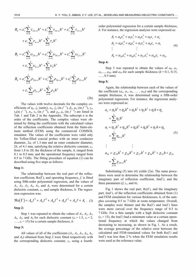
Fig. 1 shows the real part, Re(Γ), and the imaginary part, Im(Γ), of the reflection coefficients obtained from (1) and FEM simulation for various thicknesses, h, of the sam-ples covering 0.5 to 7 GHz at room temperature. Overall, the samples were thinner and the Re(Γ) and Im(Γ) lines were more curved over the frequency range of 0.5 to 7 GHz. For a thin sample with a high dielectric constant (εr = 15), the Im(Γ) had a minimum value at a certain opera-tional frequency at which the values changed from decreasing to increasing, as shown in Fig. 1. As a result, the average percentage of the relative error between the calculated and FEM-simulated values for both Re(Γ) and Im(Γ) was less than 2 % when the FEM simulation results were used as the reference value.
RADIOENGINEERING, VOL. 23, NO. 4, DECEMBER 2014 1019
0.5 1 2 3 4 5 6 70.2
0.4
0.6
0.8
1
f (GHz)
e()
r = 2
h = 0.1 mm
h = 0.2 mm
h = 0.3 mm
h = 0.4 mm
h = 0.5 mm
0.5 1 2 3 4 5 6 7-1
-0.8
-0.6
-0.4
-0.2
0
f (GHz)
m
()
r = 2
h = 0.1 mm
h = 0.2 mm
h = 0.3 mm
h = 0.4 mm
h = 0.5 mm
0.5 1 2 3 4 5 6 7-1
-0.5
0
0.5
1
f (GHz)
e()
r = 15
h = 0.1 mm
h = 0.2 mm
h = 0.3 mm
h = 0.4 mm
h = 0.5 mm
0.5 1 2 3 4 5 6 7-1
-0.9
-0.8
-0.7
-0.6
-0.5
-0.4
-0.3
-0.2
f (GHz)
m
()
r = 15
h = 0.1 mm
h = 0.2 mm
h = 0.3 mm
h = 0.4 mm
h = 0.5 mm
Fig. 1. Variations in Re(Γ)
and Im(Γ) with frequency, f, for samples with various thicknesses, h: (Note: ---- Eq. (1); -•- FEM simulation).
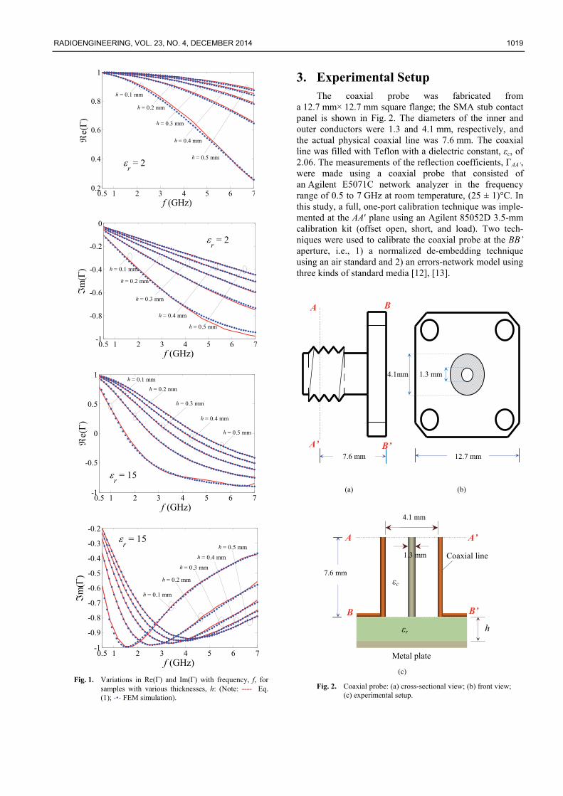
3. Experimental Setup The coaxial probe was fabricated from
a 12.7 mm× 12.7 mm square flange; the SMA stub contact panel is shown in Fig. 2. The diameters of the inner and outer conductors were 1.3 and 4.1 mm, respectively, and the actual physical coaxial line was 7.6 mm. The coaxial line was filled with Teflon with a dielectric constant, εc, of 2.06. The measurements of the reflection coefficients, ΓAA’, were made using a coaxial probe that consisted of an Agilent E5071C network analyzer in the frequency range of 0.5 to 7 GHz at room temperature, (25 ± 1)°C. In this study, a full, one-port calibration technique was imple-mented at the AA′ plane using an Agilent 85052D 3.5-mm calibration kit (offset open, short, and load). Two tech-niques were used to calibrate the coaxial probe at the BB’ aperture, i.e., 1) a normalized de-embedding technique using an air standard and 2) an errors-network model using three kinds of standard media [12], [13].
(a) (b)
(c)
Fig. 2. Coaxial probe: (a) cross-sectional view; (b) front view; (c) experimental setup.
1.3 mm 4.1mm
12.7 mm
B’
B
A’
A
7.6 mm
A A’
B B’
7.6 mm
4.1 mm
Coaxial line
Metal plate
h εr
εc
1.3 mm
1020 K. Y. YOU, Z. ABBAS, C.Y. LEE, ET AL., MODELING AND MEASURING DIELECTRIC CONSTANTS …
3.1 Normalized De-embedding Technique
In this work, a normalized de-embedding formulation (6) was used to calibrate the coaxial probe, and the formu-lation can be expressed as:
_Γ Γ Air FEM
BB AAAir
, (6)
where ΓAir is the reflection coefficient measurements for air at plane AA’, and ΓAir_FEM is the standard values of the air reflection coefficients at plane BB’, obtained by using the finite element method (COMSOL simulator). Later, the reflection coefficient, ΓBB
,, was measured with the aperture of the probe placed against a two-layer medium, and the first layered medium to be tested was a thin sample with thickness, h, and the second layered medium was the con-ducting plate. As is well known, the standing wave error is not taken into account in normalized de-embedding cali-bration techniques. The standing wave that occurred in the coaxial line was caused mainly by fringing effects at the probe aperture, which was in direct contact with the sam-ple. The standing wave effect can be ignored when the length of the operational quarter wave, λ/4, in the coaxial line is equal to or larger than the physical length, z, of the coaxial line. In this study, the error effect in the probe calibration can be neglected up to 7 GHz, the operational frequency at which λ/4 = c/(4f√εc) ≈ 7.6 mm, which is equal to the physical length (z = 7.6 mm) of the probe being studied.
3.2 Network Error Techniques
The network error relationship between the measured reflection coefficient, ΓBB’, and the actual reflection coeffi-cient, ΓAA
,, for the sample being tested can be written as a bilinear equation [11], [12]:
2
3 1
AABB
AA
C
C C
(7)
where C1, C2, and C3 are unknown complex calibration coefficients that were determined and optimized by using three calibration standards. In this study, air, liquid metha-nol, and pure water were used as the standards. Equation (7) can be rewritten as a linear expression:
1 2 3BB BB AA AAC C C . (8)
Let ΓBB’_Air, ΓBB’_Methanol , and ΓBB’_Water represent the known reflection coefficients for the air, methanol, and water standards, which terminate at the aperture plane BB’, while, ΓAA’_Air, ΓAA’_Methanol , and ΓAA’_Water are the measured reflection coefficients for air, methanol, and water at port AA’. Three sets of linear equations were developed and written in matrix form as:
_ _ _ 1
_ _ _ 2
_ _ _ 3
_
_
_
1
1
1
BB Air BB Air AA Air
BB Methanol BB Methanol AA Methanol
BB Water BB Water AA Water
AA Air
AA Methanol
AA Water
C
C
C
(9)
The values of ΓBB’_Air, ΓBB’_Methanol , and ΓBB’_Water at the aperture (plane BB’) for the air, methanol, and water were obtained from FEM simulation. In the simulation, the rela-tive permittivity, εr, of air was unity. The relative permit-tivities, εr, of methanol and water were computed by the Cole-Cole model as:
11
sr
j
. (10)
Methanol had parameters of εs = 33.7, ε∞ = 4.45, τ = 4.95·10-11 s, and α = 0.036, and water had εs = 78.6, ε∞ = 4.22, τ = 8.8·10-12 s, and α = 0.013 [13]. Equation (9) was solved by using a Gaussian elimination routine. Once the values of C1, C2, and C3 were obtained, the calibrated reflection coefficient, ΓBB
,, of the thin sample backed by the conducting plate can be calculated by using (7). The accu-racy of the network error calibration depended on the similarities between the values of εr obtained from (10) and the measured standard liquids. In this study, a short stan-dard was not involved in the probe calibration. The reason was that the interference at the aperture of the probe was terminated by short circuits, which directly affected the measured ΓBB’ due to the shorter length of study probe’s coaxial line (plane AA’ and BB’ is closed). The above con-dition caused the open (air) and short standards to fail to maintain 180o of phase separation throughout the opera-tional frequency range (especially at low operational fre-quencies).
4. Inverse Trial Function In this work, after various functions were tried, two
trial functions were recommended since both of the func-tions were able to provide more stable inverse results for all operating frequencies (0.5 to 7 GHz). Trial function (11a) represents the deviation of the ratio Re(Γ)/Im(Γ). Function (11b) is sum of the two deviation terms, i.e., the linear deviation term and the second term is the same as in function (11a). The predicted values of relative dielectric constant, εr’, of the thin sample were obtained by mini-mizing the difference between the measured reflection coefficient, ΓBB’, and the calculated Γ using (1) and by referring to the trial function, Λ:

RADIOENGINEERING, VOL. 23, NO. 4, DECEMBER 2014 1021
1
e e
m m
DataBB
BB
(11a)
or
1
m m
e e
m m
BBData
BB
BB
(11b)
MATLAB’s ‘fzero’ command was used to determine the zero routine. The initial approximate value in the nu-merical prediction was 5. The value of the relative dielec-tric constant, εr’, of the thin sample was influenced by the real part of the reflection coefficient, Re(Γ), and, equally important, by the imaginary reflection coefficient, Im(Γ). For instance, the variations in the Re(Γ) and Im(Γ) of the probe with frequency, f, and relative dielectric constant, εr’, for the sample with the thickness of 0.2 mm backed by a metallic plate are shown in Fig. 3.
0
5
10
15 1
2
3
4
5
6
7
-1
-0.5
0
0.5
1
f (GHz)r
h = 0.2 mm
e( )
e()
-0.6
-0.4
-0.2
0
0.2
0.4
0.6
0.8
0
5
10
15 0
2
4
6
8
-1
-0.8
-0.6
-0.4
-0.2
0
f (GHz)
h = 0.2 mm
r
m
()
m()
-0.9
-0.8
-0.7
-0.6
-0.5
-0.4
-0.3
-0.2
Fig. 3. Variation in Re(Γ) and Im(Γ) of water at 26°C with
frequency f and inner radial of probe a.
5. Results and Discussion To validate the results of the study, a thin layer of
propan-1-ol liquid backed by metallic plate was measured using the experimental setup, as shown in Fig. 4.
Fig. 4. Measurements of thin layer of propan-1-ol liquid aided
by the x-y transition platform.
The reflection coefficient measurements (Re(Γ), Im(Γ), and Re(Γ)/Im(Γ)) of propan-1-ol liquid at 4 GHz were compared with the results obtained from finite ele-ment computation and (1) are shown in Fig. 5. The thick-ness of the propan-1-ol liquid layer was adjusted accurately based on the distance that the metallic plate moved away from the aperture of the probe in the propan-1-ol liquid using the x-y transition. The value of relative permittivity (εr = 4.49 – j 2.77) of propan-1-ol in the simulation and in the calculation was obtained from infinite propan-1-ol liquid measurement using a Keysight (formerly Agilent) 85070D dielectric probe.
0.1 0.2 0.3 0.4 0.5
-0.6
-0.4
-0.2
0
0.2
0.4
0.6
e()
m()
h (mm)
FEM simulationsEquation (1)Measured data
0.1 0.2 0.3 0.4 0.5-1.8
-1.5
-1
-0.5
0
e()/m()
h (mm) Fig. 5. Variation in Re(Γ), Im(Γ), and Re(Γ)/Im(Γ) of propan-
1-ol liquid (εr = 4.49 – j 2.77) with layer thickness h for 4 GHz at room temperature.
x-y transition
VNA
Propan-1-ol
Coaxial probe
1022 K. Y. YOU, Z. ABBAS, C.Y. LEE, ET AL., MODELING AND MEASURING DIELECTRIC CONSTANTS …
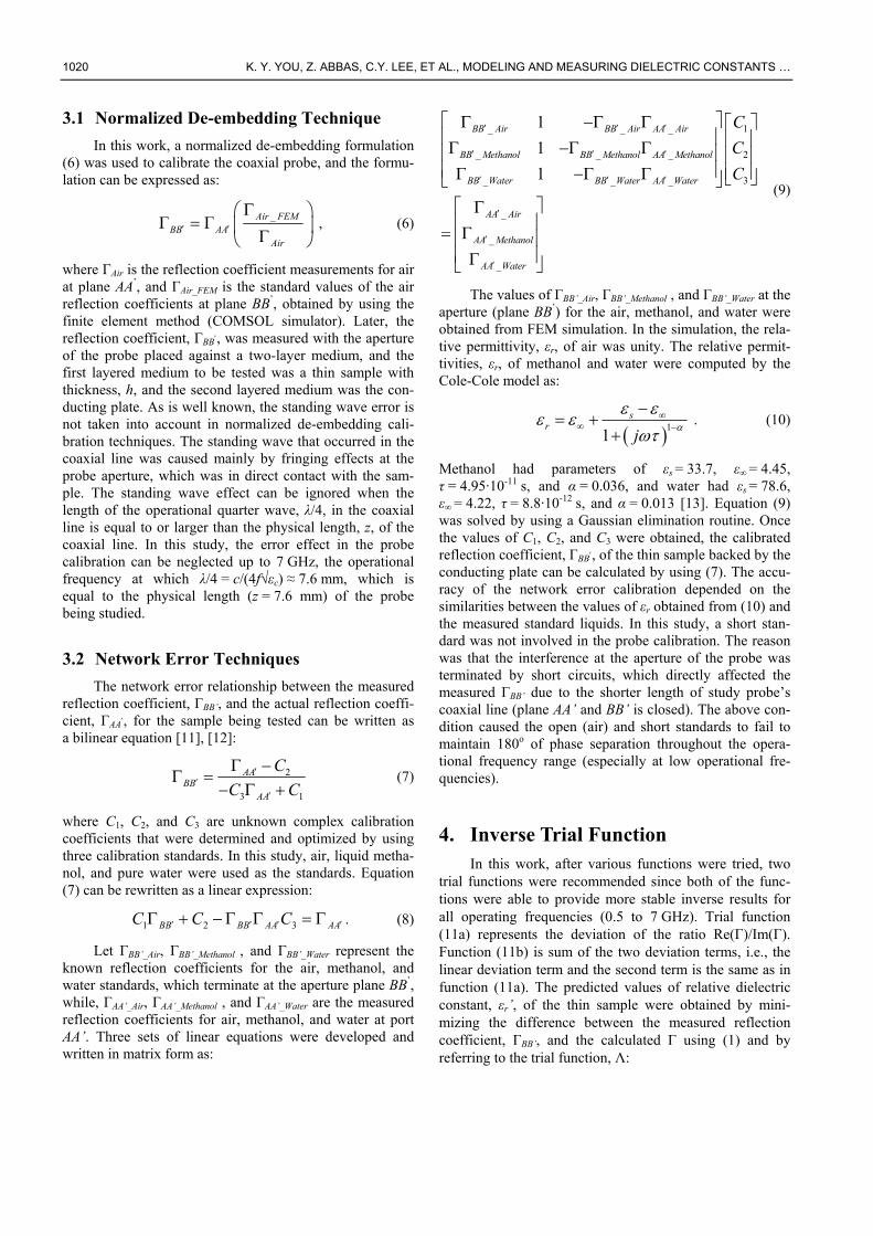
The absolute errors in the measured reflection coeffi-cient were based on the difference between the measure-ments and the results calculated by (1), as shown in Fig. 6(a). The absolute error may have been caused by the sensitive measurements and high uncertainty in the con-trolled environment for the smaller-scale thickness of pro-pan-1-ol liquid. The relative dielectric constant, εr’, which was calculated from the measured reflection coefficient using (1) and trial function (11a), is shown in Fig. 6(b). The inverse values of εr’ were found to be in relatively good agreement with the reference data, especially for h ≥ 0.2 mm.
0.1 0.2 0.3 0.4 0.50
0.01
0.02
0.03
0.04
0.05
0.06
0.07
h (mm)
Abs
olut
e er
ror
|e()|
|m()||(e()/m()]|
0.1 0.2 0.3 0.4 0.53.5
4
4.5
5
5.5
h (mm)
r ,
Inverse resultsReference line
(a) (b)
Fig. 6. (a) Variation in absolute measurement errors. (b) Corresponding inverse values of εr’ for the thick-ness of the propan-1-ol liquid backed by metallic plate at 4 GHz.
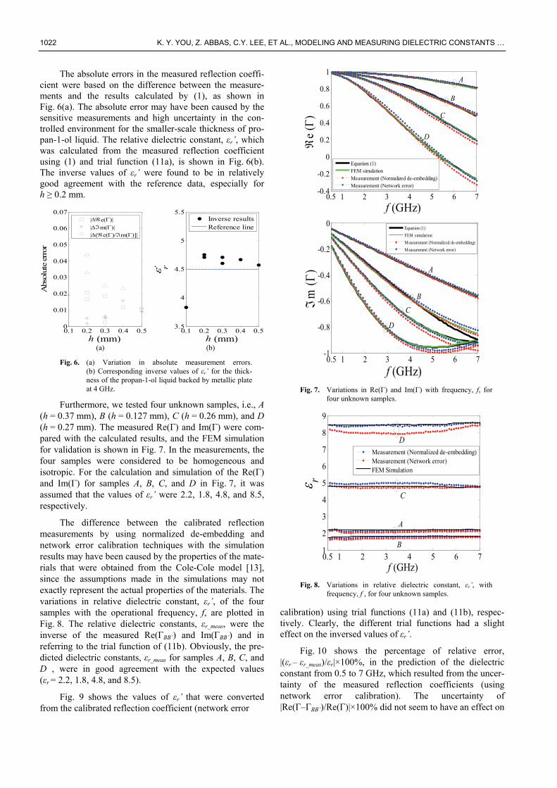
Furthermore, we tested four unknown samples, i.e., A (h = 0.37 mm), B (h = 0.127 mm), C (h = 0.26 mm), and D (h = 0.27 mm). The measured Re(Γ)
and Im(Γ) were com-pared with the calculated results, and the FEM simulation for validation is shown in Fig. 7. In the measurements, the four samples were considered to be homogeneous and isotropic. For the calculation and simulation of the Re(Γ)
and Im(Γ) for samples A, B, C, and D in Fig. 7, it was assumed that the values of εr’ were 2.2, 1.8, 4.8, and 8.5, respectively.
The difference between the calibrated reflection measurements by using normalized de-embedding and network error calibration techniques with the simulation results may have been caused by the properties of the mate-rials that were obtained from the Cole-Cole model [13], since the assumptions made in the simulations may not exactly represent the actual properties of the materials. The variations in relative dielectric constant, εr’, of the four samples with the operational frequency, f, are plotted in Fig. 8. The relative dielectric constants, εr_meas, were the inverse of the measured Re(ΓBB’)
and Im(ΓBB’) and in referring to the trial function of (11b). Obviously, the pre-dicted dielectric constants, εr_meas for samples A, B, C, and D , were in good agreement with the expected values (εr = 2.2, 1.8, 4.8, and 8.5).
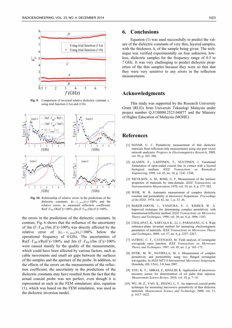
Fig. 9 shows the values of εr’ that were converted from the calibrated reflection coefficient (network error
0.5 1 2 3 4 5 6 7-0.4
-0.2
0
0.2
0.4
0.6
0.8
1
e
()
f (GHz)
Equation (1)FEM simulationMeasurement (Normalized de-embedding)Measurement (Network error)
C
B
A
D
0.5 1 2 3 4 5 6 7-1
-0.8
-0.6
-0.4
-0.2
0
m
()
f (GHz)
Equation (1)
FEM simulation
Measurement (Normalized de-embedding)
Measurement (Network error)
A
B
C
D
Fig. 7. Variations in Re(Γ) and Im(Γ) with frequency, f, for
four unknown samples.
0.5 1 2 3 4 5 6 71
2
3
4
5
6
7
8
9
r
f (GHz)
Measurement (Normalized de-embedding)Measurement (Network error)FEM Simulation
C
D
A
B
Fig. 8. Variations in relative dielectric constant, εr’, with
frequency, f , for four unknown samples.
calibration) using trial functions (11a) and (11b), respec-tively. Clearly, the different trial functions had a slight effect on the inversed values of εr’.
Fig. 10 shows the percentage of relative error, |(εr – εr_meas)/εr|×100%, in the prediction of the dielectric constant from 0.5 to 7 GHz, which resulted from the uncer-tainty of the measured reflection coefficients (using network error calibration). The uncertainty of |Re(Γ–ΓBB’)/Re(Γ)|×100% did not seem to have an effect on
RADIOENGINEERING, VOL. 23, NO. 4, DECEMBER 2014 1023
0.5 1 2 3 4 5 6 71
2
3
4
5
6
7
8
9
f (GHz)
r ,
Using trial function (11a)Using trial function (11b)
D
B
C
A
Fig. 9. Comparison of inversed relative dielectric constant, εr’
using trial function (11a) and (11b).
1 2 3 4 5 6 70
2
4
6
f (GHz)
Err
or (
%)
| e( - BB
,) / e() |
| m( - BB
,) / m() |
| (r -
r meas) /
r |
1 2 3 4 5 6 70
2
4
6
f (GHz)
Err
or (
%)
1 2 3 4 5 6 70
2
4
6
f (GHz)
Err
or (
%)
1 2 3 4 5 6 70
2
4
6
f (GHz)
Err
or (
%)
Sample A Sample B
Sample C Sample D
Fig. 10. Relationship of relative errors in the predictions of the
dielectric constants, |(εr - εr_meas)/εr|×100% and the relative errors in measured reflection coefficient, Re(Γ-ΓBB’)/Re(Γ)|×100% ,|Im (Γ-ΓBB’)/Im (Γ)|×100%.
the errors in the predictions of the dielectric constants. In contrast, Fig. 6 shows that the influence of the uncertainty of |Im (Γ–ΓBB’)/Im (Γ)|×100% was directly affected by the relative error of |(εr – εr_meas)/εr|×100% below the operational frequency of 4 GHz. The uncertainties of Re(Γ–ΓBB’)/Re(Γ)|×100% and |Im (Γ–ΓBB’)/Im (Γ)|×100% were caused mainly by the quality of the measurements, which could have been affected by various factors, such as cable movements and small air gaps between the surfaces of the samples and the aperture of the probe. In addition, to the effects of the errors on the measurements of the reflec-tion coefficient, the uncertainty in the predictions of the dielectric constants may have resulted from the fact that the actual coaxial probe was not perfect, even though it is represented as such in the FEM simulation; also, equation (1), which was based on the FEM simulation, was used as the dielectric inversion model.
6. Conclusions Equation (1) was used successfully to predict the val-
ues of the dielectric constants of very thin, layeredsamples, with the thickness, h, of the sample being given. The tech-nique was verified experimentally on four unknown, low-loss, dielectric samples for the frequency range of 0.5 to 7 GHz. It was very challenging to predict dielectric prop-erties of the thin samples because they were so thin that they were very sensitive to any errors in the reflection measurements.
Acknowledgments
This study was supported by the Research University Grant (RUG) from Universiti Teknologi Malaysia under project number Q.J130000.2523.04H77 and the Ministry of Higher Education of Malaysia (MOHE).
References
[1] HASAR, U. C. Permittivity measurement of thin dielectric materials from reflection-only measurements using one-port vector network analyzers. Progress in Electromagnetics Research, 2009, vol. 95, p. 365–380.
[2] ALANEN, E., LAHTINEN, T., NUUTINEN, J. Variational formulation of open-ended coaxial line in contact with a layered biological medium. IEEE Transactions on Biomedical Engineering, 1998, vol. 45, no. 10, p. 1241–1248.
[3] NICOLSON, A. M., ROSS, G. F. Measurement of the intrinsic properties of materials by time-domain. IEEE Transactions on Instrumentation Measurement, 1970, vol. 19, no. 4, p. 377–382.
[4] WEIR, W. B. Automatic measurement of complex dielectric constant and permeability at microwave frequencies. Proceedings of the IEEE, 1974, vol. 62, no. 1, p. 33–36.
[5] BAKER-JARVIS, J., VANZURA, E. J., KISSICK W. A. Improved technique for determining complex permittivity with transmission/reflection method. IEEE Transactions on Microwave Theory and Techniques, 1990, vol. 38, no. 8, p. 1096–1103.
[6] CHALAPAT, K., SARVALA K., LI, J., PARAOANU, G. S. Wide reference-plane invariant method for measuring electromagnetic parameters of materials. IEEE Transactions on Microwave Theory and Techniques, 2009, vol. 57, no. 9, p. 2257–2267.
[7] IATROU, C. T., CAVENAGO, M. Field analysis of rectangular waveguide open junction. IEEE Transactions on Microwave Theory and Techniques, 1997, vol. 45, no. 2, p. 165–172.
[8] HYDE, M. W., HAVRILLA, M. J. Measurement of complex permittivity and permeability using two flanged rectangular waveguides. In IEEE/MTT-S International Microwave Symposium. Honolulu, (HI, USA), 3-8 June 2007.
[9] YOU, K. Y., ABBAS, Z., KHALID, K. Application of microwave moisture sensor for determination of oil palm fruit ripeness. Measurement Science Review, 2010, vol. 10, p. 7–14.
[10] WU, M. Z., YAO, X., ZHANG, L. Y. An improved coaxial probe technique for measuring microwave permittivity of thin dielectric materials. Measurement Science and Technology, 2000, vol. 11, p. 1617–1622.

1024 K. Y. YOU, Z. ABBAS, C.Y. LEE, ET AL., MODELING AND MEASURING DIELECTRIC CONSTANTS …
[11] KRASZEWSKI, A., STUCHLY, M. A., STUCHLY, S. S. ANA calibration method for measurements of dielectric properties. IEEE Transactions on Instrumentation Measurement, 1983, vol. 32, no. 2, p. 385–386.
[12] GHANNOUCHI, F. M., MOHAMMADI A. The Six-Port Tech-nique with Microwave and Wireless Applications. Norwood: Artech House, 2009, p. 113–117.
[13] BLACKHAM, D. V., POLLARD, R. D. An improved technique for permittivity measurements using a coaxial probe. IEEE Trans-actions on Instrumentation Measurement, 1997, vol. 46, no. 5, p. 1093–1099.
[14] JONSCHER, A. K. Dielectric Relaxation in Solids, London: Chelsea Dielectrics Press, 1983.
Appendix
A1 A2 ( f -1) A3 ( f
-2) A4 ( f -3) A5 ( f
-4) A6 ( f -5)
η0 1.137678976 α0 -7.174384419×10⁻¹⁰ β0 5.84953605×10⁻¹⁹ γ0 -7.300482213×10⁻²⁹ σ0 -9.69945174×10-39 χ0 1.387481423×10-48
η1 -2.496804026
(mm-1) α1
1.400425896×10⁻⁸
(mm-1) β1
-1.321455272×10⁻¹⁷
(mm-1) γ1
3.013030643×10⁻²⁷
(mm-1) σ1
-1.440657387×10-37
(mm-1) χ1
-6.506718621×10⁻⁸
(mm-1)
η2 16.217964374
(mm-2) α2
-9.479166403×10⁻⁸
(mm-2) β2
9.558192050×10⁻¹⁷
(mm-2) γ2
-2.573560518×10⁻²⁶
(mm-2) σ2
2.125220478×10-36
(mm-2) χ2
-2.841452872×10-47
(mm-2)
η3 -49.577642405
(mm-3) α3
2.977152619×10⁻⁷
(mm-3) β3
-3.116385419×10⁻¹⁶
(mm-3) γ3
9.058064131×10⁻²⁶
(mm-3) σ3
-8.78239945×10-36
(mm-3) χ3
2.228982801×10-46
(mm-3)
η4 72.890175760
(mm-4) α4
-4.462811331×10⁻⁷
(mm-4) β4
4.785010214×10⁻¹⁶
(mm-4) γ4
-1.452655788×10⁻²⁵
(mm-4) σ4
1.520783268×10⁻³⁵
(mm-4) χ4
-4.637419948×10-46
(mm-4)
η5 -41.638803263
(mm-5) α5
2.587036734×10⁻⁷
(mm-5)
β5 -2.820454316×10⁻¹⁶
(mm-5) γ5
8.804307457×10⁻²⁶
(mm-5) σ5
-9.63745234×10-36
(mm-5) χ5
3.208686456×10-46
(mm-5)
η6 -8.476869639×10⁻² α6 3.968551071×10⁻¹⁰ β6 -2.514545622×10⁻¹⁹ γ6 -3.165556019×10⁻²⁹ σ6 1.961656879×10-38 χ6 -1.614889391×10-48
η7 1.628592641
(mm-1) α7
-8.468731665×10⁻⁹
(mm-1) β7
6.989649526×10⁻¹⁸
(mm-1) γ7
-8.542478603×10⁻²⁸
(mm-1) σ7
-1.06174372×10-37
(mm-1) χ7
1.545499884×10-47
(mm-1)
η8 -10.944264964
(mm-2) α8
5.990178923×10⁻⁸
(mm-2) β8
-5.459100314×10⁻¹⁷
(mm-2) γ8
1.076836252×10⁻²⁶
(mm-2) σ8
-2.435513478×10-37
(mm-2) χ8
-4.754630520×10-47
(mm-2)
η9 34.250339804
(mm-3) α9
-1.932872547×10⁻⁷
(mm-3) β9
1.853323360×10⁻¹⁶
(mm-3) γ9
-4.300991531×10⁻²⁶
(mm-3)
σ9 2.544011484×10-36
(mm-3) χ9
4.310243495×10-47
(mm-3)
η10 -51.243553259
(mm-4) α10
2.951774599×10⁻⁷
(mm-4) β10
-2.918349732×10⁻¹⁶
(mm-4) γ10
7.348767626×10⁻²⁶
(mm-4) σ10
-5.551898575×10-36
(mm-4) χ10
3.925554480×10-47
(mm-4)
η11 29.672536501
(mm-5) α11
-1.734582527×10⁻⁷
(mm-5) β11
1.750175001×10⁻¹⁶
(mm-5) γ11
-4.627140958×10⁻²⁶
(mm-5) σ11
3.922264336×10-36
(mm-5) χ11
-6.47483795×10-47
(mm-5)
η12 1.198533901×10⁻² α12 -3.913268461×10⁻¹¹ β12 -2.429981611×10⁻²⁰ γ12 3.217569122×10⁻²⁹ σ12 -7.28932584×10-39 χ12 4.765811711×10-49
η13 -2.617748871×10⁻¹
(mm-1) α13
1.127463728×10⁻⁹
(mm-1) β13
-3.18246809×10⁻¹⁹
(mm-1) γ13
-2.458348130×10⁻²⁸
(mm-1) σ13
7.999395281×10-38
(mm-1) χ13
-5.944504765×10-48
(mm-1)
η14 1.869925598
(mm-2) α14
-8.885874782×10⁻⁹
(mm-2) β14
4.739124892×10⁻¹⁸
(mm-2) γ14
3.655001739×10⁻²⁸
(mm-2) σ14
-3.216837424×10-37
(mm-2) χ14
2.809325398×10-47
(mm-2)
η15 -6.064922598
(mm-3) α15
3.030102394×10⁻⁸
(mm-3) β15
-1.959032525×10⁻¹⁷
(mm-3) γ15
1.225128749×10⁻²⁷
(mm-3) σ15
6.035792922×10-37
(mm-3) χ15
-6.552445075×10-47
(mm-3)
η16 9.29057809
(mm-4) α16
-4.784895412×10⁻⁸
(mm-4) β16
3.39568064×10⁻¹⁷
(mm-4) γ16
-4.140019751×10⁻²⁷
(mm-4) σ16
-5.086583342×10-37
(mm-4) χ16
7.602488997×10-47
(mm-4)
η17 -5.470450232
(mm-5) α17
2.875392541×10⁻⁸
(mm-5) β17
-2.154742793×10⁻¹⁷
(mm-5) γ17
3.328573492×10⁻²⁷
(mm-5) σ17
1.351965847×10-37
(mm-5) χ17
-3.511505529×10-47
(mm-5)
η18 -3.553651117×10⁻⁴ α18 -6.960658498×10⁻¹³ β18 5.132942667×10⁻²¹ γ18 -3.228471732×10⁻³⁰ σ18 6.1987191×10-40 χ18 -3.766348885×10-50
η19 1.127323101×10⁻²
(mm-1) α19
-2.570618736×10⁻¹¹
(mm-1) β19
-3.812202685×10⁻²⁰
(mm-1) γ19
3.694556223×10⁻²⁹
(mm-1) σ19
-8.133263075×10-39
(mm-1) χ19
5.306760013×10-49
(mm-1)
η20 -9.146445647×10⁻²
(mm-2) α20
3.099260942×10⁻¹⁰
(mm-2) β20
4.502034254×10⁻²⁰
(mm-2) γ20
-1.567581658×10⁻²⁸
(mm-2)
σ20 4.033848910×10-38
(mm-2) χ20
-2.815315443×10-48
(mm-2)
η21 3.159763324×10⁻¹
(mm-3) α21
-1.227925332×10⁻⁹
(mm-3)
β21 2.507133070×10⁻¹⁹
(mm-3) γ21
3.186318282×10⁻²⁸
(mm-3) σ21
-9.890012523×10-38
(mm-3) χ21
7.358225420×10-48
(mm-3)
η22 -5.024342061×10⁻¹
(mm-4) α22
2.093334242×10⁻⁹
(mm-4) β22
-7.582190607×10⁻¹⁹
(mm-4) γ22
-3.079346108×10⁻²⁸
(mm-4) σ22
1.209501746×10-37
(mm-4) χ22
-9.565310006×10-48
(mm-4)
η23 3.031657214×10⁻¹
(mm-5) α23
-1.317250312×10⁻⁹
(mm-5) β23
5.941497062×10⁻¹⁹
(mm-5) γ23
1.099717314×10⁻²⁸
(mm-5) σ23
-5.906593807×10-38
(mm-5) χ23
4.951049919×10-48
(mm-5)
η24 2.060325131×10⁻⁷
α24 6.13810462×10⁻¹⁴ β24 -1.538769797×10⁻²² γ24 8.197907995×10⁻³² σ24 -1.478240481×10-41 χ24 8.689655504×10-52
η25 -1.263437901×10⁻⁴
(mm-1) α25
-2.290879414×10⁻¹³
(mm-1) β25
1.650856406×10⁻²¹
(mm-1) γ25
-1.068403377×10⁻³⁰
(mm-1) σ25
2.109967011×10-40
(mm-1) χ25
-1.30935851×10-50
(mm-1)
η26 1.295088408×10⁻³
(mm-2) α26
-1.90266234×10⁻¹²
(mm-2) β26
-6.353196305×10⁻²¹
(mm-2) γ26
5.258504738×10⁻³⁰
(mm-2) σ26
-1.130328088×10-39
(mm-2) χ26
7.342262493×10-50
(mm-2)
η27 -4.906190645×10⁻³
(mm-3) α27 1.249950704×10⁻¹¹
(mm-3)
β27 1.0938935570×10⁻²⁰
(mm-3)
γ27 -1.277751969×10⁻²⁹
(mm-3)
σ27 2.977052018×10-39
(mm-3)
χ27 -2.009974235×10-49
(mm-3)
η28 8.194138917×10⁻³
(mm-4) α28 -2.521870626×10⁻¹¹
(mm-4)
β28 -7.548539233×10⁻²¹
(mm-4)
γ28 1.5470641676×10⁻²⁹
(mm-4)
σ28 -3.89444317×10-39
(mm-4)
χ28 2.717871721×10-49
(mm-4)
η29 -5.096381229×10⁻³
(mm-5)
α29 1.727670528×10⁻¹¹
(mm-5)
β29 7.878796629×10⁻²²
(mm-5)
γ29 -7.4740476512×10⁻³⁰
(mm-5)
σ29 2.026440077×10-39
(mm-5)
χ29 -1.455195765×10-49
(mm-5)
Tab. 1. Coefficients for Equation (2a).
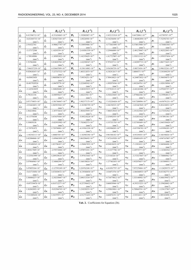
RADIOENGINEERING, VOL. 23, NO. 4, DECEMBER 2014 1025
B1 B2 ( f -1) B3 ( f
-2) B4 ( f -3) B5 ( f
-4) B6 ( f -5)
ζ0 8.413306712×10⁻² ξ0 -8.351656065×10⁻¹⁰ Ψ0 1.192802807×10⁻¹⁸ τ0 -5.432131914×10⁻²⁸ ν0 8.66728061×10-38 ρ0 -4.5789707×10-48
ζ1 -8.652445733×10⁻¹
(mm-1) ξ1
1.025827244×10⁻⁸
(mm-1) Ψ1
-1.69226950×10⁻¹⁷
(mm-1)
τ1 8.318256698×10⁻²⁷
(mm-1) ν1
-1.404482894×10-36
(mm-1) ρ1
7.732592743×10-47
(mm-1)
ζ2 2.916522763
(mm-2) ξ2
-4.900627747×10⁻⁸
(mm-2) Ψ2
9.130959406×10⁻¹⁷
(mm-2) τ2
-4.773663498×10⁻²⁶
(mm-2) ν2
8.378015908×10-36
(mm-2) ρ2
-4.736883505×10-46
(mm-2)
ζ3 -3.137172588
(mm-3) ξ3
1.14293539×10⁻⁷
(mm-3) Ψ3
-2.410581539×10⁻¹⁶
(mm-3)
τ3 1.329466089×10⁻²⁵
(mm-3) ν3
-2.401270467×10⁻³⁵
(mm-3) ρ3
1.382522843×10-45
(mm-3)
ζ4 -1.709149086
(mm-4) ξ4
-1.305052822×10⁻⁷
(mm-4)
Ψ4 3.142359429×10⁻¹⁶
(mm-4)
τ4 -1.817727007×10⁻²⁵
(mm-4) ν4
3.358333112×10⁻³⁵
(mm-4) ρ4
-1.959357434×10-45
(mm-4)
ζ5 3.767862684
(mm-5) ξ5
5.834828784×10⁻⁸
(mm-5) Ψ5
-1.622500347×10⁻¹⁶
(mm-5)
τ5 9.797655711×10⁻²⁶
(mm-5) ν5
-1.843897715×10⁻³⁵
(mm-5) ρ5
1.086773425×10-45
(mm-5)
ζ6 -7.966357239×10⁻² ξ6 4.528687099×10⁻¹⁰ Ψ6 -9.330114082×10⁻¹⁹ τ6 3.936384739×10⁻²⁸ ν6 -5.90573454×10-38 ρ6 2.990152241×10-48
ζ7 9.929630347×10⁻¹
(mm-1) ξ7
-7.327337322×10⁻⁹
(mm-1) Ψ7
1.403212075×10⁻¹⁷
(mm-1) τ7
-6.342412617×10⁻²⁷
(mm-1)
ν7 1.0084571×10-36
(mm-1) ρ7
-5.341044259×10-47
(mm-1)
ζ8 -4.650435459
(mm-2) ξ8
3.988950674×10⁻⁸
(mm-2) Ψ8
-7.99534251×10⁻¹⁷
(mm-2) τ8
3.789418823×10⁻²⁶
(mm-2) ν8
-6.244073032×10-36
(mm-2) ρ8
3.396954075×10-46
(mm-2)
ζ9 10.4837820524
(mm-3) ξ9
-1.04470778×10⁻⁷
(mm-3) Ψ9
2.222608542×10⁻¹⁶
(mm-3) τ9
-1.092074366×10⁻²⁵
(mm-3)
ν9 1.843264761×10⁻³⁵
(mm-3) ρ9
-1.020154984×10-45
(mm-3)
ζ10 -11.425418839
(mm-4) ξ10
1.344820448×10⁻⁷
(mm-4) Ψ10
-3.041019233×10⁻¹⁶
(mm-4) τ10
1.537810115×10⁻²⁵
(mm-4) ν10
-2.641265206×10⁻³⁵
(mm-4) ρ10
1.479243757×10-45
(mm-4)
ζ11 4.796161336
(mm-5) ξ11
-6.848950237×10⁻⁸
(mm-5) Ψ11
1.64223392×10⁻¹⁶
(mm-5) τ11
-8.502625685×10⁻²⁶
(mm-5) ν11
1.479866386×10⁻³⁵
(mm-5) ρ11
-8.359964813×10-46
(mm-5)
ζ12 2.071774853×10⁻² ξ12 -1.501746867×10⁻¹⁰ Ψ12 1.982377175×10⁻¹⁹ τ12 -7.152226424×10⁻²⁹ ν12 9.817208094×10-39 ρ12 -4.654791231×10-49
ζ13 -2.916624851×10⁻¹
(mm-1) ξ13
2.282953944×10⁻⁹
(mm-1) Ψ13
-3.181903759×10⁻¹⁸
(mm-1) τ13
1.246194525×10⁻²⁷
(mm-1) ν13
-1.831667845×10-37
(mm-1) ρ13
9.201418052×10-48
(mm-1)
ζ14 1.564210842
(mm-2) ξ14
-1.307574416×10⁻⁸
(mm-2) Ψ14
1.903835959×10⁻¹⁷
(mm-2) τ14
-7.806515018×10⁻²⁷
(mm-2)
ν14 1.191523564×10-36
(mm-2) ρ14
-6.173352562×10-47
(mm-2)
ζ15 -4.113754388
(mm-3) ξ15
3.653679384×10⁻⁸
(mm-3) Ψ15
-5.505210224×10⁻¹⁷
(mm-3) τ15
2.325492555×10⁻²⁶
(mm-3) ν15
-3.632831622×10-36
(mm-3) ρ15
1.917091301×10-46
(mm-3)
ζ16 5.350859158
(mm-4) ξ16
-5.025935902×10⁻⁸
(mm-4) Ψ16
7.782482573×10⁻¹⁷
(mm-4) τ16
-3.357331783×10⁻²⁶
(mm-4)
ν16 5.327505449×10-36
(mm-4) ρ16
-2.845358428×10-46
(mm-4)
ζ17 -2.759781872
(mm-5) ξ17
2.728788081×10⁻⁸
(mm-5) Ψ17
-4.319561238×10⁻¹⁷
(mm-5) τ17
1.892904205×10⁻²⁶
(mm-5) ν17
-3.037596782×10-36
(mm-5) ρ17
1.635996285×10-46
(mm-5)
ζ18 -1.582542111×10⁻³ ξ18 1.04005705×10⁻¹¹ Ψ18 -1.182903396×10⁻²⁰ τ18 3.901588182×10⁻³⁰ ν18 -4.95339455×10-40 ρ18 2.168196026×10-50
ζ19 2.422804846×10⁻²
(mm-1) ξ19
-1.699463899×10⁻¹⁰
(mm-1) Ψ19
2.065296692×10⁻¹⁹
(mm-1) τ19
-7.472163928×10⁻²⁹
(mm-1)
ν19 1.036081659×10-38
(mm-1) ρ19
-4.947167007×10-49
(mm-1)
ζ20 -1.391488565×10⁻¹
(mm-2) ξ20
1.023706267×10⁻⁹
(mm-2) Ψ20
-1.296867855×10⁻¹⁸
(mm-2) τ20
4.924018639×10⁻²⁸
(mm-2) ν20
-7.13583412×10-38
(mm-2) ρ20
3.546946404×10-48
(mm-2)
ζ21 3.883617049×10⁻¹
(mm-3) ξ21
-2.970734046×10⁻⁹
(mm-3) Ψ21
3.870974101×10⁻¹⁸
(mm-3) τ21
-1.513277786×10⁻²⁷
(mm-3)
ν21 2.24975577×10-37
(mm-3) ρ21
-1.143402562×10-47
(mm-3)
ζ22 -5.325561999×10⁻¹
(mm-4) ξ22
4.209529618×10⁻⁹
(mm-4) Ψ22
-5.597615443×10⁻¹⁸
(mm-4) τ22
2.23144326×10⁻²⁷
(mm-4)
ν22 -3.372527047×10-37
(mm-4) ρ22
1.738004962×10-47
(mm-4)
ζ23 2.879846965×10⁻¹
(mm-5) ξ23
-2.34068299×10⁻⁹
(mm-5)
Ψ23 3.160150824×10⁻¹⁸
(mm-5) τ23
-1.277462455×10⁻²⁷
(mm-5)
ν23 1.952870457×10-37
(mm-5) ρ23
-1.015890931×10-47
(mm-5)
ζ24 3.478055264×10⁻⁵ ξ24 -2.127593249×10⁻¹³ Ψ24 2.224762248×10⁻²² τ24 -6.818567797×10⁻³² ν24 7.957270484×10-42 ρ24 -3.124299375×10-52
ζ25 -5.631715056×10⁻⁴
(mm-1) ξ25
3.672929672×10⁻¹²
(mm-1) Ψ25
-4.139360454×10⁻²¹
(mm-1) τ25
1.416071576×10⁻³⁰
(mm-1) ν25
-1.864360933×10-40
(mm-1) ρ25
8.433382773×10-51
(mm-1)
ζ26 3.368464237×10⁻³
(mm-2) ξ26
-2.292358447×10⁻¹¹
(mm-2) Ψ26
2.696313534×10⁻²⁰
(mm-2) τ26
-9.734779012×10⁻³⁰
(mm-2)
ν26 1.353148992×10-39
(mm-2) ρ26
-6.466199472×10-50
(mm-2)
ζ27 -9.697354478×10⁻³
(mm-3) ξ27
6.816712277×10⁻¹¹
(mm-3) Ψ27
-8.237396432×10⁻²⁰
(mm-3) τ27
3.068039944×10⁻²⁹
(mm-3) ν27
-4.393315231×10-39
(mm-3) ρ27
2.159420882×10-49
(mm-3)
ζ28 1.363042892×10⁻²
(mm-4) ξ28
-9.832944745×10⁻¹¹
(mm-4) Ψ28
1.210350253×10⁻¹⁹
(mm-4) τ28
-4.599654961×10⁻²⁹
(mm-4) ν28
6.709669741×10-39
(mm-4) ρ28
-3.354157967×10-49
(mm-4)
ζ29 -7.521005628×10⁻³
(mm-5) ξ29
5.54197071×10⁻¹¹
(mm-5) Ψ29
-6.912751653×10⁻²⁰
(mm-5) τ29
2.664076191×10⁻²⁹
(mm-5) ν29
-3.93516411×10-39
(mm-5) ρ29
1.989183898×10-49
(mm-5)
Tab. 2. Coefficients for Equation (2b).