Embed Size (px)
Citation preview
Stephen L. Campbell, Jean-Philippe Chancelier andRamine Nikoukhah
Modeling and Simulation inScilab/Scicos

Mathematics Subject Classification (2000): 01-01, 04-01, 11 Axx, 26-01
Library of Congress Control Number: 2005930797
ISBN-10: 0-387-27802-8ISBN-13: 978-0387278025
Printed on acid-free paper.
© 2006 Springer Science + Business Media, Inc.All rights reserved. This work may not be translated or copied in whole or in part without thewritten permission of the publisher (Springer Science+Business Media, Inc., 233 Spring Street,New York, NY 10013, USA), except for brief excerpts in connection with reviews or scholarlyanalysis. Use in connection with any form of information storage and retrieval, electronicadaption, computer software, or by similar or dissimilar methodology now known or hereafterdeveloped is forbidden. The use in this publication of trade names, trademarks, service marks, andsimilar terms, even if they are not identified as such, is not to be taken as an expression of opinionas to whether or not they are subject to proprietary rights.
Printed in the United States of America. (BPR/HAM)
9 8 7 6 5 4 3 2 1
springeronline.com
Preface
Scilab (http://www.scilab.org) is a free open-source software package for scientific com-putation. It includes hundreds of general purpose and specialized functions for numericalcomputation, organized in libraries called toolboxes that cover such areas as simulation,optimization, systems and control, and signal processing. These functions reduce consid-erably the burden of programming for scientific applications.
One important Scilab toolbox is Scicos. Scicos (http://www.scicos.org) providesa block-diagram graphical editor for the construction and simulation of dynamical sys-tems. Scilab/Scicos is the only open-source alternative to commercial packages for dy-namical system modeling and simulation packages such as MATLAB/Simulink and MA-TRIXx/SystemBuild. Widely used at universities and engineering schools, Scilab/Scicosis gaining ground in industrial environments. This is due in part to the creation of aninternational consortium in 2003 that a number of large and small companies have joined.The consortium is responsible for providing well-tested and documented releases for vari-ous platforms and coordinates the development of the core product and toolboxes, whichis done by research groups, in particular, at INRIA1 and ENPC.2 Currently there are over10,000 monthly Scilab downloads from http://www.scilab.org alone.
Scilab includes a full user’s manual, which is available with search capabilities in ahelp window. All commands, their syntax, and simple illustrative examples are given.While very useful in finding out the details of a particular command, this manual does notprovide a tutorial on the philosophy of either Scilab or Scicos. Nor does it address how touse several of these commands together in the solution of a technical problem.
The objective of this book is to provide a tutorial for the use of Scilab/Scicos with aspecial emphasis on modeling and simulation tools. While it will provide useful informationto experienced users, it is designed to be accessible to beginning users from a variety ofdisciplines. Students [33] and academic and industrial scientists and engineers should findit useful. The discussion includes some information on modeling and simulation in order toassist the reader in deciding which simulation tools might be most useful to them. Everysoftware environment has its special features, some would say quirks, that experiencedusers automatically take into account but often prove confusing to beginning users. Wehave tried to point these out where appropriate.
The book is divided into two parts. The first part concerns Scilab and includes atutorial covering the language features, the data structures and specialized functions fordoing graphics, importing and exporting data, interfacing with external routines, etc. It
1 Institut National de Recherche en Informatique et en Automatique2 Ecole Nationale des Ponts et des Chaussees

VI Preface
also covers in detail Scilab numerical solvers for ODEs (ordinary differential equations) andDAE’s (differential-algebraic equations). Even though the emphasis is placed on modelingand simulation applications, this part provides a global view of the product.
The second part is dedicated to modeling and simulation of dynamical systems in Sci-cos. Scicos provides a block-diagram editor for constructing models. This type of modelingtool is widely used in industry because it provides a means for constructing modular andreusable models. This part contains a detailed description of the editor and its usage,which is illustrated through numerous examples. It also covers advanced subjects such asconstructing new blocks and batch simulation. Code generation and debugging are othertopics covered. Finally, a new extension of Scicos is discussed. This extension allows theuse of components described by the Modelica (http://www.modelica.org) language.
There have been several previous books concerning Scilab. Most of these have been inFrench [18, 3, 2, 1, 25] and dealt with earlier versions of Scilab, as in [16]. This book isunique in a number of ways. It is the first to deal with the new Scilab 3.1 version. Thisbook is also the first to focus on simulation and modeling. It is also the first to put a majoremphasis on Scicos and discuss Scicos in depth.
The source of all the examples presented in this book can be downloaded fromhttp://www.scicos.org.
Finally, a large number of people have supported us in many ways. We would especiallylike to thank our wives, Gail Campbell and Homa Nikoukhah, and our parents, Aline andRene Chancelier, for their support in this and everything else we do.
Steve CampbellJean-Philippe ChancelierRamine Nikoukhah
Contents
Part I Scilab
1 General Information . . . . . . . . . . . . . . . . . . . . . . . . . . . . . . . . . . . . . . . . . . . . . . . . . 31.1 What Is Scilab? . . . . . . . . . . . . . . . . . . . . . . . . . . . . . . . . . . . . . . . . . . . . . . . . . . . 31.2 How to Start? . . . . . . . . . . . . . . . . . . . . . . . . . . . . . . . . . . . . . . . . . . . . . . . . . . . . . 4
1.2.1 Installation . . . . . . . . . . . . . . . . . . . . . . . . . . . . . . . . . . . . . . . . . . . . . . . . . 41.2.2 First Steps . . . . . . . . . . . . . . . . . . . . . . . . . . . . . . . . . . . . . . . . . . . . . . . . . 41.2.3 Line Editor . . . . . . . . . . . . . . . . . . . . . . . . . . . . . . . . . . . . . . . . . . . . . . . . . 51.2.4 Documentation . . . . . . . . . . . . . . . . . . . . . . . . . . . . . . . . . . . . . . . . . . . . . 6
1.3 Typical Usage . . . . . . . . . . . . . . . . . . . . . . . . . . . . . . . . . . . . . . . . . . . . . . . . . . . . . 61.4 Scilab on the Web . . . . . . . . . . . . . . . . . . . . . . . . . . . . . . . . . . . . . . . . . . . . . . . . . 7
2 Introduction to Scilab . . . . . . . . . . . . . . . . . . . . . . . . . . . . . . . . . . . . . . . . . . . . . . . 92.1 Scilab Objects . . . . . . . . . . . . . . . . . . . . . . . . . . . . . . . . . . . . . . . . . . . . . . . . . . . . 11
2.1.1 Matrix Construction and Manipulation . . . . . . . . . . . . . . . . . . . . . . . . . 122.1.2 Strings . . . . . . . . . . . . . . . . . . . . . . . . . . . . . . . . . . . . . . . . . . . . . . . . . . . . . 172.1.3 Boolean Matrices . . . . . . . . . . . . . . . . . . . . . . . . . . . . . . . . . . . . . . . . . . . . 192.1.4 Polynomial Matrices . . . . . . . . . . . . . . . . . . . . . . . . . . . . . . . . . . . . . . . . . 202.1.5 Sparse Matrices . . . . . . . . . . . . . . . . . . . . . . . . . . . . . . . . . . . . . . . . . . . . . 212.1.6 Lists . . . . . . . . . . . . . . . . . . . . . . . . . . . . . . . . . . . . . . . . . . . . . . . . . . . . . . . 222.1.7 Functions . . . . . . . . . . . . . . . . . . . . . . . . . . . . . . . . . . . . . . . . . . . . . . . . . . 26
2.2 Scilab Programming . . . . . . . . . . . . . . . . . . . . . . . . . . . . . . . . . . . . . . . . . . . . . . . 272.2.1 Branching . . . . . . . . . . . . . . . . . . . . . . . . . . . . . . . . . . . . . . . . . . . . . . . . . . 282.2.2 Iterations . . . . . . . . . . . . . . . . . . . . . . . . . . . . . . . . . . . . . . . . . . . . . . . . . . 292.2.3 Scilab Functions . . . . . . . . . . . . . . . . . . . . . . . . . . . . . . . . . . . . . . . . . . . . . 312.2.4 Debugging Programs . . . . . . . . . . . . . . . . . . . . . . . . . . . . . . . . . . . . . . . . . 35
2.3 Input and Output Functions . . . . . . . . . . . . . . . . . . . . . . . . . . . . . . . . . . . . . . . . 372.3.1 Display of Variables . . . . . . . . . . . . . . . . . . . . . . . . . . . . . . . . . . . . . . . . . 372.3.2 Formatted Input and Output . . . . . . . . . . . . . . . . . . . . . . . . . . . . . . . . . 382.3.3 Input Output in Binary Mode . . . . . . . . . . . . . . . . . . . . . . . . . . . . . . . . 402.3.4 Accessing the Host System . . . . . . . . . . . . . . . . . . . . . . . . . . . . . . . . . . . 422.3.5 Graphical User Interface . . . . . . . . . . . . . . . . . . . . . . . . . . . . . . . . . . . . . 43
2.4 Scilab Graphics . . . . . . . . . . . . . . . . . . . . . . . . . . . . . . . . . . . . . . . . . . . . . . . . . . . 482.4.1 Basic Graphing . . . . . . . . . . . . . . . . . . . . . . . . . . . . . . . . . . . . . . . . . . . . . 482.4.2 Graphic Tour . . . . . . . . . . . . . . . . . . . . . . . . . . . . . . . . . . . . . . . . . . . . . . . 492.4.3 Graphics Objects . . . . . . . . . . . . . . . . . . . . . . . . . . . . . . . . . . . . . . . . . . . . 53
VIII Contents
2.4.4 Scilab Graphics and LATEX. . . . . . . . . . . . . . . . . . . . . . . . . . . . . . . . . . . . 562.4.5 Old Graphics Style . . . . . . . . . . . . . . . . . . . . . . . . . . . . . . . . . . . . . . . . . . 60
2.5 Interfacing . . . . . . . . . . . . . . . . . . . . . . . . . . . . . . . . . . . . . . . . . . . . . . . . . . . . . . . . 622.5.1 Linking Code . . . . . . . . . . . . . . . . . . . . . . . . . . . . . . . . . . . . . . . . . . . . . . . 632.5.2 Writing an Interface . . . . . . . . . . . . . . . . . . . . . . . . . . . . . . . . . . . . . . . . . 662.5.3 Dynamic Loading . . . . . . . . . . . . . . . . . . . . . . . . . . . . . . . . . . . . . . . . . . . 69
3 Modeling and Simulation in Scilab . . . . . . . . . . . . . . . . . . . . . . . . . . . . . . . . . . . 733.1 Types of Models . . . . . . . . . . . . . . . . . . . . . . . . . . . . . . . . . . . . . . . . . . . . . . . . . . . 73
3.1.1 Ordinary Differential Equations . . . . . . . . . . . . . . . . . . . . . . . . . . . . . . . 733.1.2 Boundary Value Problems . . . . . . . . . . . . . . . . . . . . . . . . . . . . . . . . . . . . 743.1.3 Difference Equations . . . . . . . . . . . . . . . . . . . . . . . . . . . . . . . . . . . . . . . . . 753.1.4 Differential Algebraic Equations . . . . . . . . . . . . . . . . . . . . . . . . . . . . . . . 763.1.5 Hybrid Systems . . . . . . . . . . . . . . . . . . . . . . . . . . . . . . . . . . . . . . . . . . . . . 77
3.2 Simulation Tools . . . . . . . . . . . . . . . . . . . . . . . . . . . . . . . . . . . . . . . . . . . . . . . . . . 783.2.1 Ordinary Differential Equations . . . . . . . . . . . . . . . . . . . . . . . . . . . . . . . 783.2.2 Boundary Value Problems . . . . . . . . . . . . . . . . . . . . . . . . . . . . . . . . . . . . 903.2.3 Difference Equations . . . . . . . . . . . . . . . . . . . . . . . . . . . . . . . . . . . . . . . . . 953.2.4 Differential Algebraic Equations . . . . . . . . . . . . . . . . . . . . . . . . . . . . . . . 983.2.5 Hybrid Systems . . . . . . . . . . . . . . . . . . . . . . . . . . . . . . . . . . . . . . . . . . . . . 100
4 Optimization . . . . . . . . . . . . . . . . . . . . . . . . . . . . . . . . . . . . . . . . . . . . . . . . . . . . . . . . 1074.1 Comments on Optimization and Solving Nonlinear Equations . . . . . . . . . . . 1074.2 General Optimization . . . . . . . . . . . . . . . . . . . . . . . . . . . . . . . . . . . . . . . . . . . . . . 1084.3 Solving Nonlinear Equations . . . . . . . . . . . . . . . . . . . . . . . . . . . . . . . . . . . . . . . . 1124.4 Nonlinear Least Squares . . . . . . . . . . . . . . . . . . . . . . . . . . . . . . . . . . . . . . . . . . . . 1134.5 Parameter Fitting . . . . . . . . . . . . . . . . . . . . . . . . . . . . . . . . . . . . . . . . . . . . . . . . . 1174.6 Linear and Quadratic Programming . . . . . . . . . . . . . . . . . . . . . . . . . . . . . . . . . 119
4.6.1 Linear Programs . . . . . . . . . . . . . . . . . . . . . . . . . . . . . . . . . . . . . . . . . . . . 1194.6.2 Quadratic Programs . . . . . . . . . . . . . . . . . . . . . . . . . . . . . . . . . . . . . . . . . 1204.6.3 Semidefinite Programs . . . . . . . . . . . . . . . . . . . . . . . . . . . . . . . . . . . . . . . 120
4.7 Differentiation Utilities . . . . . . . . . . . . . . . . . . . . . . . . . . . . . . . . . . . . . . . . . . . . . 1204.7.1 Higher Derivatives . . . . . . . . . . . . . . . . . . . . . . . . . . . . . . . . . . . . . . . . . . . 122
5 Examples . . . . . . . . . . . . . . . . . . . . . . . . . . . . . . . . . . . . . . . . . . . . . . . . . . . . . . . . . . . . 1255.1 Modeling and Simulation of an N -Link Pendulum . . . . . . . . . . . . . . . . . . . . . 125
5.1.1 Equations of Motion of the N -Link Pendulum. . . . . . . . . . . . . . . . . . . 1265.1.2 Generated Code and Simulation . . . . . . . . . . . . . . . . . . . . . . . . . . . . . . . 1305.1.3 Maple Code . . . . . . . . . . . . . . . . . . . . . . . . . . . . . . . . . . . . . . . . . . . . . . . . 133
5.2 Modeling and Simulation of a Car . . . . . . . . . . . . . . . . . . . . . . . . . . . . . . . . . . . 1355.2.1 Basic Model . . . . . . . . . . . . . . . . . . . . . . . . . . . . . . . . . . . . . . . . . . . . . . . . 1355.2.2 Equations of Motion . . . . . . . . . . . . . . . . . . . . . . . . . . . . . . . . . . . . . . . . . 1365.2.3 Simulation Model . . . . . . . . . . . . . . . . . . . . . . . . . . . . . . . . . . . . . . . . . . . 1385.2.4 Scilab Implementation . . . . . . . . . . . . . . . . . . . . . . . . . . . . . . . . . . . . . . . 1395.2.5 Simulation Result . . . . . . . . . . . . . . . . . . . . . . . . . . . . . . . . . . . . . . . . . . . 141
5.3 Open-Loop Control to Swing Up a Pendulum . . . . . . . . . . . . . . . . . . . . . . . . . 1425.3.1 Model . . . . . . . . . . . . . . . . . . . . . . . . . . . . . . . . . . . . . . . . . . . . . . . . . . . . . 1425.3.2 Control Problem Formulation . . . . . . . . . . . . . . . . . . . . . . . . . . . . . . . . . 1425.3.3 Optimization Problem . . . . . . . . . . . . . . . . . . . . . . . . . . . . . . . . . . . . . . . 1435.3.4 Implementation in Scilab . . . . . . . . . . . . . . . . . . . . . . . . . . . . . . . . . . . . . 145

Contents IX
5.4 Parameter Fitting and Implicit Models . . . . . . . . . . . . . . . . . . . . . . . . . . . . . . . 1475.4.1 Mathematical Model . . . . . . . . . . . . . . . . . . . . . . . . . . . . . . . . . . . . . . . . . 1485.4.2 Scilab Implementation . . . . . . . . . . . . . . . . . . . . . . . . . . . . . . . . . . . . . . . 148
Part II Scicos
6 Introduction . . . . . . . . . . . . . . . . . . . . . . . . . . . . . . . . . . . . . . . . . . . . . . . . . . . . . . . . . 159
7 Getting Started . . . . . . . . . . . . . . . . . . . . . . . . . . . . . . . . . . . . . . . . . . . . . . . . . . . . . . 1637.1 Construction of a Simple Diagram . . . . . . . . . . . . . . . . . . . . . . . . . . . . . . . . . . . 163
7.1.1 Running Scicos . . . . . . . . . . . . . . . . . . . . . . . . . . . . . . . . . . . . . . . . . . . . . . 1637.1.2 Editing a Model . . . . . . . . . . . . . . . . . . . . . . . . . . . . . . . . . . . . . . . . . . . . . 1637.1.3 Diagram Simulation . . . . . . . . . . . . . . . . . . . . . . . . . . . . . . . . . . . . . . . . . 1657.1.4 Changing Block Parameters . . . . . . . . . . . . . . . . . . . . . . . . . . . . . . . . . . 166
7.2 Symbolic Parameters and Context . . . . . . . . . . . . . . . . . . . . . . . . . . . . . . . . . . . 1697.3 Hierarchy . . . . . . . . . . . . . . . . . . . . . . . . . . . . . . . . . . . . . . . . . . . . . . . . . . . . . . . . . 173
7.3.1 Placing a Super Block in a Diagram . . . . . . . . . . . . . . . . . . . . . . . . . . . 1737.3.2 Editing a Super Block . . . . . . . . . . . . . . . . . . . . . . . . . . . . . . . . . . . . . . . 174
7.4 Save and Load . . . . . . . . . . . . . . . . . . . . . . . . . . . . . . . . . . . . . . . . . . . . . . . . . . . . 1757.4.1 Scicos File Formats . . . . . . . . . . . . . . . . . . . . . . . . . . . . . . . . . . . . . . . . . . 1757.4.2 Super Block and Palette . . . . . . . . . . . . . . . . . . . . . . . . . . . . . . . . . . . . . . 176
7.5 Synchronism and Special Blocks . . . . . . . . . . . . . . . . . . . . . . . . . . . . . . . . . . . . . 176
8 Scicos Formalism . . . . . . . . . . . . . . . . . . . . . . . . . . . . . . . . . . . . . . . . . . . . . . . . . . . . 1798.1 Activation Signal . . . . . . . . . . . . . . . . . . . . . . . . . . . . . . . . . . . . . . . . . . . . . . . . . . 179
8.1.1 Block Activation . . . . . . . . . . . . . . . . . . . . . . . . . . . . . . . . . . . . . . . . . . . . 1798.1.2 Activation Generation . . . . . . . . . . . . . . . . . . . . . . . . . . . . . . . . . . . . . . . 181
8.2 Inheritance . . . . . . . . . . . . . . . . . . . . . . . . . . . . . . . . . . . . . . . . . . . . . . . . . . . . . . . 1828.3 Always Active Blocks . . . . . . . . . . . . . . . . . . . . . . . . . . . . . . . . . . . . . . . . . . . . . . 1838.4 Constant Blocks . . . . . . . . . . . . . . . . . . . . . . . . . . . . . . . . . . . . . . . . . . . . . . . . . . . 1848.5 Conditional Blocks . . . . . . . . . . . . . . . . . . . . . . . . . . . . . . . . . . . . . . . . . . . . . . . . 184
9 Scicos Blocks . . . . . . . . . . . . . . . . . . . . . . . . . . . . . . . . . . . . . . . . . . . . . . . . . . . . . . . . 1899.1 Block Behavior . . . . . . . . . . . . . . . . . . . . . . . . . . . . . . . . . . . . . . . . . . . . . . . . . . . . 189
9.1.1 External Activation . . . . . . . . . . . . . . . . . . . . . . . . . . . . . . . . . . . . . . . . . . 1899.1.2 Always Activation . . . . . . . . . . . . . . . . . . . . . . . . . . . . . . . . . . . . . . . . . . . 1919.1.3 Internal Zero-Crossing . . . . . . . . . . . . . . . . . . . . . . . . . . . . . . . . . . . . . . . 192
9.2 Blocks Inside Palettes . . . . . . . . . . . . . . . . . . . . . . . . . . . . . . . . . . . . . . . . . . . . . . 1929.3 Modifying Block Parameters . . . . . . . . . . . . . . . . . . . . . . . . . . . . . . . . . . . . . . . . 1939.4 Super Block and Scifunc . . . . . . . . . . . . . . . . . . . . . . . . . . . . . . . . . . . . . . . . . . 193
9.4.1 Super Blocks . . . . . . . . . . . . . . . . . . . . . . . . . . . . . . . . . . . . . . . . . . . . . . . 1939.4.2 Scifunc . . . . . . . . . . . . . . . . . . . . . . . . . . . . . . . . . . . . . . . . . . . . . . . . . . . . 194
9.5 Constructing New Basic Blocks . . . . . . . . . . . . . . . . . . . . . . . . . . . . . . . . . . . . . 1949.5.1 Interfacing Function . . . . . . . . . . . . . . . . . . . . . . . . . . . . . . . . . . . . . . . . . 1959.5.2 Computational Function . . . . . . . . . . . . . . . . . . . . . . . . . . . . . . . . . . . . . 1979.5.3 Saving New Blocks . . . . . . . . . . . . . . . . . . . . . . . . . . . . . . . . . . . . . . . . . . 207
9.6 Constructing and Loading a New Palette . . . . . . . . . . . . . . . . . . . . . . . . . . . . . 207
X Contents
10 Examples . . . . . . . . . . . . . . . . . . . . . . . . . . . . . . . . . . . . . . . . . . . . . . . . . . . . . . . . . . . . 20910.1 Predator Prey Model . . . . . . . . . . . . . . . . . . . . . . . . . . . . . . . . . . . . . . . . . . . . . . 20910.2 Control Application . . . . . . . . . . . . . . . . . . . . . . . . . . . . . . . . . . . . . . . . . . . . . . . . 21010.3 Signal Processing Application . . . . . . . . . . . . . . . . . . . . . . . . . . . . . . . . . . . . . . . 21310.4 Queuing Systems . . . . . . . . . . . . . . . . . . . . . . . . . . . . . . . . . . . . . . . . . . . . . . . . . . 21610.5 Neuroscience Application . . . . . . . . . . . . . . . . . . . . . . . . . . . . . . . . . . . . . . . . . . . 21810.6 A Fluid Model of TCP-Like Behavior . . . . . . . . . . . . . . . . . . . . . . . . . . . . . . . . 22010.7 Interactive GUI . . . . . . . . . . . . . . . . . . . . . . . . . . . . . . . . . . . . . . . . . . . . . . . . . . . 221
11 Batch Processing in Scilab . . . . . . . . . . . . . . . . . . . . . . . . . . . . . . . . . . . . . . . . . . . 22711.1 Piloting Scicos via Scilab Commands . . . . . . . . . . . . . . . . . . . . . . . . . . . . . . . . . 227
11.1.1 Function scicosim . . . . . . . . . . . . . . . . . . . . . . . . . . . . . . . . . . . . . . . . . . 22811.1.2 Function scicos simulate . . . . . . . . . . . . . . . . . . . . . . . . . . . . . . . . . . . 232
11.2 Data Sharing . . . . . . . . . . . . . . . . . . . . . . . . . . . . . . . . . . . . . . . . . . . . . . . . . . . . . 23311.2.1 Context Variables . . . . . . . . . . . . . . . . . . . . . . . . . . . . . . . . . . . . . . . . . . . 23411.2.2 Input/Output Files . . . . . . . . . . . . . . . . . . . . . . . . . . . . . . . . . . . . . . . . . . 23411.2.3 Global Variables . . . . . . . . . . . . . . . . . . . . . . . . . . . . . . . . . . . . . . . . . . . . 236
11.3 Examples . . . . . . . . . . . . . . . . . . . . . . . . . . . . . . . . . . . . . . . . . . . . . . . . . . . . . . . . . 23711.4 Steady-State Solution and Linearization . . . . . . . . . . . . . . . . . . . . . . . . . . . . . . 243
11.4.1 Scilab Function steadycos . . . . . . . . . . . . . . . . . . . . . . . . . . . . . . . . . . . 24711.4.2 Scilab Function lincos . . . . . . . . . . . . . . . . . . . . . . . . . . . . . . . . . . . . . . 248
12 Code Generation . . . . . . . . . . . . . . . . . . . . . . . . . . . . . . . . . . . . . . . . . . . . . . . . . . . . 25312.1 Code Generation Procedure . . . . . . . . . . . . . . . . . . . . . . . . . . . . . . . . . . . . . . . . . 25312.2 Limitations . . . . . . . . . . . . . . . . . . . . . . . . . . . . . . . . . . . . . . . . . . . . . . . . . . . . . . . 257
12.2.1 Continuous-Time Activation . . . . . . . . . . . . . . . . . . . . . . . . . . . . . . . . . . 25712.2.2 Synchronicism . . . . . . . . . . . . . . . . . . . . . . . . . . . . . . . . . . . . . . . . . . . . . . 258
12.3 A Look Inside . . . . . . . . . . . . . . . . . . . . . . . . . . . . . . . . . . . . . . . . . . . . . . . . . . . . . 25812.4 Some Pitfalls . . . . . . . . . . . . . . . . . . . . . . . . . . . . . . . . . . . . . . . . . . . . . . . . . . . . . 26012.5 Applications . . . . . . . . . . . . . . . . . . . . . . . . . . . . . . . . . . . . . . . . . . . . . . . . . . . . . . 263
13 Debugging . . . . . . . . . . . . . . . . . . . . . . . . . . . . . . . . . . . . . . . . . . . . . . . . . . . . . . . . . . . 26713.1 Error Messages . . . . . . . . . . . . . . . . . . . . . . . . . . . . . . . . . . . . . . . . . . . . . . . . . . . . 267
13.1.1 Block Errors . . . . . . . . . . . . . . . . . . . . . . . . . . . . . . . . . . . . . . . . . . . . . . . . 26713.1.2 Errors During Numerical Integration . . . . . . . . . . . . . . . . . . . . . . . . . . . 26813.1.3 Other Errors . . . . . . . . . . . . . . . . . . . . . . . . . . . . . . . . . . . . . . . . . . . . . . . . 269
13.2 Debugging Tools . . . . . . . . . . . . . . . . . . . . . . . . . . . . . . . . . . . . . . . . . . . . . . . . . . 26913.3 Examples . . . . . . . . . . . . . . . . . . . . . . . . . . . . . . . . . . . . . . . . . . . . . . . . . . . . . . . . . 270
13.3.1 Log File . . . . . . . . . . . . . . . . . . . . . . . . . . . . . . . . . . . . . . . . . . . . . . . . . . . . 27113.3.2 Animation . . . . . . . . . . . . . . . . . . . . . . . . . . . . . . . . . . . . . . . . . . . . . . . . . . 271
14 Implicit Scicos and Modelica . . . . . . . . . . . . . . . . . . . . . . . . . . . . . . . . . . . . . . . . 27314.1 Introduction . . . . . . . . . . . . . . . . . . . . . . . . . . . . . . . . . . . . . . . . . . . . . . . . . . . . . . 27314.2 Internally Implicit Blocks . . . . . . . . . . . . . . . . . . . . . . . . . . . . . . . . . . . . . . . . . . . 27514.3 Implicit Blocks . . . . . . . . . . . . . . . . . . . . . . . . . . . . . . . . . . . . . . . . . . . . . . . . . . . . 275
14.3.1 Scicos Editor . . . . . . . . . . . . . . . . . . . . . . . . . . . . . . . . . . . . . . . . . . . . . . . 27614.3.2 Scicos Compiler . . . . . . . . . . . . . . . . . . . . . . . . . . . . . . . . . . . . . . . . . . . . . 27614.3.3 Block Construction . . . . . . . . . . . . . . . . . . . . . . . . . . . . . . . . . . . . . . . . . . 276
14.4 Example . . . . . . . . . . . . . . . . . . . . . . . . . . . . . . . . . . . . . . . . . . . . . . . . . . . . . . . . . 277
Contents XI
A Inside Scicos . . . . . . . . . . . . . . . . . . . . . . . . . . . . . . . . . . . . . . . . . . . . . . . . . . . . . . . . . 281A.1 Scicos Editor . . . . . . . . . . . . . . . . . . . . . . . . . . . . . . . . . . . . . . . . . . . . . . . . . . . . . . 281
A.1.1 Main Editor Function . . . . . . . . . . . . . . . . . . . . . . . . . . . . . . . . . . . . . . . . 281A.1.2 Structure of scs m . . . . . . . . . . . . . . . . . . . . . . . . . . . . . . . . . . . . . . . . . . . 283
A.2 Scicos Complier . . . . . . . . . . . . . . . . . . . . . . . . . . . . . . . . . . . . . . . . . . . . . . . . . . . 286A.2.1 First Compilation Stage . . . . . . . . . . . . . . . . . . . . . . . . . . . . . . . . . . . . . . 286A.2.2 Second Compilation Stage . . . . . . . . . . . . . . . . . . . . . . . . . . . . . . . . . . . . 287A.2.3 Structure of %cpr . . . . . . . . . . . . . . . . . . . . . . . . . . . . . . . . . . . . . . . . . . . . 287A.2.4 Partial Compilation . . . . . . . . . . . . . . . . . . . . . . . . . . . . . . . . . . . . . . . . . 290
A.3 Scicos Simulator . . . . . . . . . . . . . . . . . . . . . . . . . . . . . . . . . . . . . . . . . . . . . . . . . . . 291
B Scicos Blocks of Type 5 . . . . . . . . . . . . . . . . . . . . . . . . . . . . . . . . . . . . . . . . . . . . . . 293B.1 Type 5 Block for the Bouncing Ball Example . . . . . . . . . . . . . . . . . . . . . . . . . 293B.2 Animation Block for the Cart Pendulum Example . . . . . . . . . . . . . . . . . . . . . 294
C Animation Program for the Car Example . . . . . . . . . . . . . . . . . . . . . . . . . . . . 299
D Extraction Program for the LATEX Graphic Example . . . . . . . . . . . . . . . . 301
E Maple Code Used for Modeling the N-Link Pendulum . . . . . . . . . . . . . . . 303
References . . . . . . . . . . . . . . . . . . . . . . . . . . . . . . . . . . . . . . . . . . . . . . . . . . . . . . . . . . . . . . . 307
Index . . . . . . . . . . . . . . . . . . . . . . . . . . . . . . . . . . . . . . . . . . . . . . . . . . . . . . . . . . . . . . . . . . . . 309

Part I
Scilab
1
General Information
1.1 What Is Scilab?
There exist two categories of general scientific software: computer algebra systems thatperform symbolic computations, and general purpose numerical systems performing nu-merical computations and designed specifically for scientific applications. The best-knownexamples in the first category are Maple, Mathematica, Maxima, Axiom, and MuPad. Thesecond category represents a larger market dominated by MATLAB. Scilab, which is freeopen-source software, belongs to this second category.
Scilab is an interpreted language with dynamically typed objects. Scilab runs, and isavailable in binary format, for the main available platforms: Unix/Linux workstations (themain software development is performed on Linux workstations), Windows, and MacOSX.MacOSX users can also install Scilab using fink. Compiling Scilab from the source code isalso possible and is fairly straightforward.
Scilab was originally named Basile and was developed at INRIA as part of the Meta2project. Development continued under the name of Scilab by the Scilab group, which wasa team of researchers from INRIA Metalau and ENPC. Since 2004, Scilab developmenthas been coordinated by a consortium.
Scilab can be used as a scripting language to test algorithms or to perform numericalcomputations. But it is also a programming language, and the standard Scilab librarycontains around 2000 Scilab coded functions. The Scilab syntax is simple, and the useof matrices, which are the fundamental object of scientific calculus, is facilitated throughspecific functions and operators. These matrices can be of different types including real,complex, string, polynomial, and rational. Scilab programs are thus quite compact andmost of the time are smaller than their equivalents in C, C++, or Java.
Scilab is mainly dedicated to scientific computing, and it provides easy access to largenumerical libraries from such areas as linear algebra, numerical integration, and opti-mization. It is also simple to extend the Scilab environment. One can easily import newfunctionalities from external libraries into Scilab by using static or dynamic links. It isalso possible to define new data types using Scilab structures and to overload standardoperators for new data types. Numerous toolboxes that add specialized functions to Scilabare available on the official site.
Scilab also provides many visualization functionalities including 2D, 3D, contour andparametric plots, and animation. Graphics can be exported in various formats such as Gif,Postscript, Postscript-Latex, and Xfig. In addition to Scilab’s user interface functions,the Scilab Tcl/Tk interface can be used to develop sophisticated GUI’s (Graphical userinterfaces).

4 1 General Information
Scilab is a large software package containing approximately 13,000 files, more than400,000 lines of source code (in C and Fortran), 70,000 lines of Scilab code (specializedlibraries), 80,000 lines of online help, and 18,000 lines of configuration files. These filesinclude
• Elementary functions of scientific calculation;• Linear algebra, sparse matrices;• Polynomials and rational functions;• Classic and robust control, LMI optimization;• Nonlinear methods (optimization, ODE and DAE solvers, Scicos, which is a hybrid
dynamic systems modeler and simulator);• Signal processing;• Random sampling and statistics;• Graphs (algorithms, visualization);• Graphics, animation;• Parallelism using PVM;• MATLAB-to-Scilab translator;• A large number of contributions for various areas.
1.2 How to Start?
1.2.1 Installation
Scilab is available for downloading at http://www.scilab.org. The procedure for in-stalling Scilab depends on the operating system (Windows, MacOSX, Linux, or Unix),and information can be found on the website. The user has the choice between installingthe binary version (if one is available for the host system) and compiling the source ver-sion. To compile the source version, the host system must be equipped with appropriateC and Fortran compilers. For the Windows operating system, a Visual C++ compiler suf-fices because an f2c (Fortran-to-C) translator is included in the source code. Note that Cand Fortran compilers are already installed on most Linux platforms, and for other Unixsystems, if native compilers are not available, freely available GNU compilers can be used.On computers running MacOSX there is also the option of installing Scilab using fink.
In this book, SCI designates the directory in which Scilab is installed. We use theUnix notation for specifying path names. For example, SCI/routines/machine.h is the filemachine.h in the subdirectory routines. Under the Windows operating system, all the“ / ” should be replaced with “ \ ”.
Even though there are no restrictions on its use, Scilab is copyrighted; see the filelicense.txt (English) or licence.txt (French) on the website.
1.2.2 First Steps
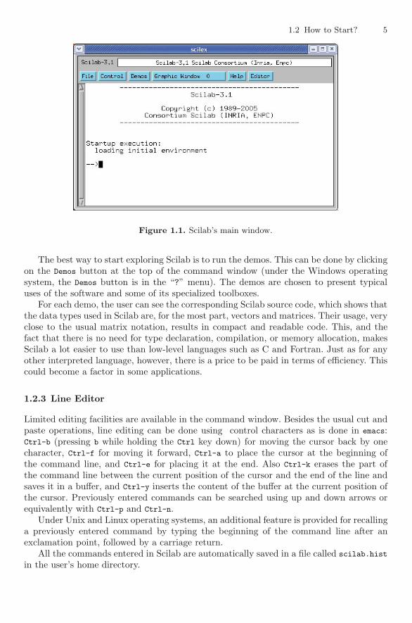
Running Scilab opens up a command window; see Figure 1.1. The look of this windowmay differ depending on the window manager.
The Scilab command window is an interactive window where the user is invited toenter a command at Scilab’s prompt (-->). The command must be validated with a car-riage return, after which Scilab executes the command and returns control to the user bydisplaying a new prompt.
1.2 How to Start? 5
Figure 1.1. Scilab’s main window.
The best way to start exploring Scilab is to run the demos. This can be done by clickingon the Demos button at the top of the command window (under the Windows operatingsystem, the Demos button is in the “?” menu). The demos are chosen to present typicaluses of the software and some of its specialized toolboxes.
For each demo, the user can see the corresponding Scilab source code, which shows thatthe data types used in Scilab are, for the most part, vectors and matrices. Their usage, veryclose to the usual matrix notation, results in compact and readable code. This, and thefact that there is no need for type declaration, compilation, or memory allocation, makesScilab a lot easier to use than low-level languages such as C and Fortran. Just as for anyother interpreted language, however, there is a price to be paid in terms of efficiency. Thiscould become a factor in some applications.
1.2.3 Line Editor
Limited editing facilities are available in the command window. Besides the usual cut andpaste operations, line editing can be done using control characters as is done in emacs:Ctrl-b (pressing b while holding the Ctrl key down) for moving the cursor back by onecharacter, Ctrl-f for moving it forward, Ctrl-a to place the cursor at the beginning ofthe command line, and Ctrl-e for placing it at the end. Also Ctrl-k erases the part ofthe command line between the current position of the cursor and the end of the line andsaves it in a buffer, and Ctrl-y inserts the content of the buffer at the current position ofthe cursor. Previously entered commands can be searched using up and down arrows orequivalently with Ctrl-p and Ctrl-n.
Under Unix and Linux operating systems, an additional feature is provided for recallinga previously entered command by typing the beginning of the command line after anexclamation point, followed by a carriage return.
All the commands entered in Scilab are automatically saved in a file called scilab.hist
in the user’s home directory.

6 1 General Information
1.2.4 Documentation
Scilab has a comprehensive online help facility, which can be consulted through the com-mands help and apropos. To consult the manual page corresponding to a Scilab function,the command help followed by the name of the function can be used. This opens up abrowser window displaying the manual page in question. The manual page contains a de-tailed description of the function and a number of examples of its usage. The examplescan be cut and pasted into Scilab’s command window to be executed. The browser, whichcan also be accessed by clicking on the help button at the top of the command window,contains a list of all the functions classified by theme in different chapters (see Fig. 1.2).The manual page of a function can then be obtained by clicking on its name.
To obtain a list of Scilab functions corresponding to a keyword, the command apropos
followed by the keyword should be used.
Figure 1.2. Help browser window.
The demos are also a good source of inspiration. They present simple examples ofScilab programming situations frequently encountered by users. The graphics demos, forexample, give an overall picture of what can be done in Scilab as far as visualization isconcerned. The demos’ source codes often provide a good starting point for developingcomplex applications.
The demos provide examples for doing graphics, signal processing, systems control,Scilab simulation (in particular, the famous bicycle example), Scicos simulation, and a lotmore.
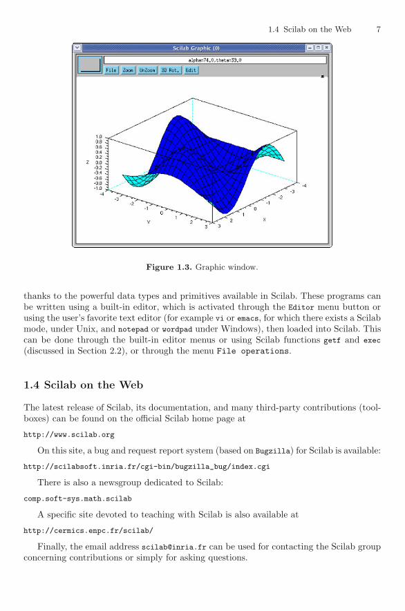
1.3 Typical Usage
A typical Scilab user spends most of his time going back and forth between Scilab anda text editor. For the most part, Scilab programs contain very few lines of instructions,
1.4 Scilab on the Web 7
Figure 1.3. Graphic window.
thanks to the powerful data types and primitives available in Scilab. These programs canbe written using a built-in editor, which is activated through the Editor menu button orusing the user’s favorite text editor (for example vi or emacs, for which there exists a Scilabmode, under Unix, and notepad or wordpad under Windows), then loaded into Scilab. Thiscan be done through the built-in editor menus or using Scilab functions getf and exec
(discussed in Section 2.2), or through the menu File operations.
1.4 Scilab on the Web
The latest release of Scilab, its documentation, and many third-party contributions (tool-boxes) can be found on the official Scilab home page at
http://www.scilab.org
On this site, a bug and request report system (based on Bugzilla) for Scilab is available:
http://scilabsoft.inria.fr/cgi-bin/bugzilla_bug/index.cgi
There is also a newsgroup dedicated to Scilab:
comp.soft-sys.math.scilab
A specific site devoted to teaching with Scilab is also available at
http://cermics.enpc.fr/scilab/
Finally, the email address [email protected] can be used for contacting the Scilab groupconcerning contributions or simply for asking questions.
2
Introduction to Scilab
The Scilab language was initially devoted to matrix operations, and scientific and engi-neering applications were its main target. But over time, it has considerably evolved, andcurrently the Scilab language includes powerful operators for manipulating a large classof basic objects.
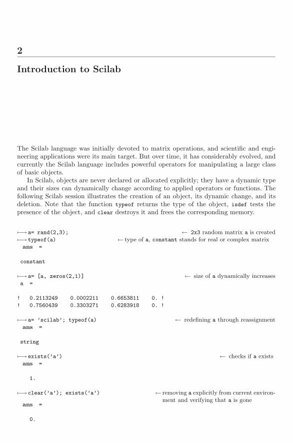
In Scilab, objects are never declared or allocated explicitly; they have a dynamic typeand their sizes can dynamically change according to applied operators or functions. Thefollowing Scilab session illustrates the creation of an object, its dynamic change, and itsdeletion. Note that the function typeof returns the type of the object, isdef tests thepresence of the object, and clear destroys it and frees the corresponding memory.
�−→ a= rand(2,3); ← 2x3 random matrix a is created�−→ typeof(a) ← type of a, constant stands for real or complex matrix
ans =
constant
�−→ a= [a, zeros(2,1)] ← size of a dynamically increasesa =
! 0.2113249 0.0002211 0.6653811 0. !
! 0.7560439 0.3303271 0.6283918 0. !
�−→ a= ’scilab’; typeof(a) ← redefining a through reassignmentans =
string
�−→ exists(’a’) ← checks if a existsans =
1.
�−→ clear(’a’); exists(’a’) ← removing a explicitly from current environ-ment and verifying that a is gone
ans =
0.
10 2 Introduction to Scilab
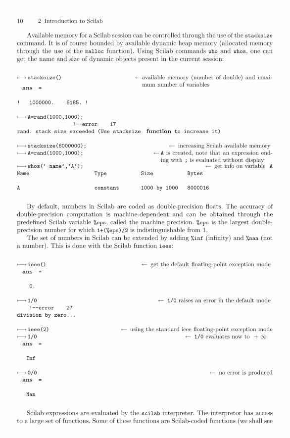
Available memory for a Scilab session can be controlled through the use of the stacksizecommand. It is of course bounded by available dynamic heap memory (allocated memorythrough the use of the malloc function). Using Scilab commands who and whos, one canget the name and size of dynamic objects present in the current session:
�−→ stacksize() ← available memory (number of double) and maxi-mum number of variables
ans =
! 1000000. 6185. !
�−→ A=rand(1000,1000);
!--error 17
rand: stack size exceeded (Use stacksize function to increase it)
�−→ stacksize(6000000); ← increasing Scilab available memory�−→ A=rand(1000,1000); ← A is created, note that an expression end-
ing with ; is evaluated without display�−→ whos(’-name’,’A’); ← get info on variable A
Name Type Size Bytes
A constant 1000 by 1000 8000016
By default, numbers in Scilab are coded as double-precision floats. The accuracy ofdouble-precision computation is machine-dependent and can be obtained through thepredefined Scilab variable %eps, called the machine precision. %eps is the largest double-precision number for which 1+(%eps)/2 is indistinguishable from 1.
The set of numbers in Scilab can be extended by adding %inf (infinity) and %nan (nota number). This is done with the Scilab function ieee:
�−→ ieee() ← get the default floating-point exception modeans =
0.
�−→ 1/0 ← 1/0 raises an error in the default mode!--error 27
division by zero...
�−→ ieee(2) ← using the standard ieee floating-point exception mode�−→ 1/0 ← 1/0 evaluates now to + ∞
ans =
Inf
�−→ 0/0 ← no error is producedans =
Nan
Scilab expressions are evaluated by the scilab interpreter. The interpretor has accessto a large set of functions. Some of these functions are Scilab-coded functions (we shall see
2.1 Scilab Objects 11
later that Scilab is a programming language), some are hard-coded functions (C or Fortrancoded). This ability of Scilab to include C or Fortran coded functions means that a largeamount of existing scientific and engineering software can be used from within Scilab.
Scilab is a rich and powerful programming environment because of this large number ofavailable functions. The users can also enrich the basic Scilab environment with their ownScilab or hard-coded functions, and moreover this can be done dynamically (hard-codedfunctions can be dynamically loaded in a running Scilab session); we shall see how thiscan be done later. Thus, toolboxes can be developed to enrich and adapt Scilab to specificneeds or areas of application.
2.1 Scilab Objects
Scilab provides users with a large variety of basic objects starting with numbers andcharacter strings up to more sophisticated objects such as booleans, polynomials, andstructures. A Scilab object is a basic object or a set of basic objects arranged in a vector,a matrix, a hypermatrix, or a structure (list).
As already mentioned, Scilab is devoted to scientific computing, and the basic objectis a two-dimensional matrix with floating-point double-precision number entries. In fact,a real scalar is nothing but a 1× 1 matrix. The next Scilab session illustrates this type ofobject. Note that some numerical constants are predefined in Scilab. Their correspondingvariable names start with %. In particular, π is %pi, and e, the base of the natural log, is%e. Note also that a:b:c gives numbers starting from a to c spaced b units apart.
�−→ a=1:0.6:3 ← a is now a scalar matrix (double)a =
! 1. 1.6 2.2 2.8 !
�−→ b=[%e,%pi] ← b is the 1x2 row vector filled with predefined values (e, π)b =
! 2.7182818 3.1415927 !
New types have been added as Scilab has evolved, but the matrix aspect has alwaysbeen kept. String matrices, boolean matrices, sparse matrices, integer matrices (int8,int16, int32), polynomial matrices, and rational matrices are now available in the stan-dard Scilab environment. Complex structures called lists (list, tlist, and mlist) are alsoavailable. Note also that functions in Scilab are considered as objects as well.
�−→ a= "Scilab" ← a 1x1 string matrixa =
Scilab
�−→ b=rand(2,2) ← a matrixb =
! 0.2113249 0.0002211 !
! 0.7560439 0.3303271 !

12 2 Introduction to Scilab
�−→ b= b>= 0.5 ← a boolean matrixb =
! F F !
! T F !
�−→ L=list(a,b) ← a listL =
L(1)
Scilab
L(2)
! F F !
! T F !
�−→ A.x = 32;A.y = %t ← a structure implemented using mlist
A =
x: 32
y: %t
�−→ a= spec(rand(3,3)) ← eigenvalues: a vector of complex numbersa =
! 1.8925237 !
! 0.1887123 + 0.0535764i !
! 0.1887123 - 0.0535764i !
It is possible to define new types in Scilab in the sense that it is possible to define objectswhose dynamic type (the value returned by typeof) is user-defined. Scilab operators, forexample the + and * operators, can be overloaded for these dynamically defined types. Thenew types are defined and implemented with tlist and mlist primitive types (see Section2.1.6).
2.1.1 Matrix Construction and Manipulation
As already pointed out, one of the goals of Scilab is to give access to matrix operationsfor any kind of matrix types. In this section we highlight general functions and operatorsthat are common to all matrix types.
A matrix in Scilab refers to one- or two-dimensional arrays, which are internally storedas a one-dimensional array (two-dimensional arrays are stored in column order). It istherefore always possible to access matrix entries with one or two indices. Vectors andscalars are stored as matrices.
Multidimensional matrices can also be used in Scilab. They are called hypermatrices.Elementary construction operators, which are overloaded for all matrix types, are the
row concatenation operator “;” and the column concatenation operator “,”. These twooperators perform the concatenation operation when used in a matrix context, that is,when they appear between “[” and “]”. All the associated entries must be of the same
2.1 Scilab Objects 13
type. Note that in the same matrix context a white space means the same thing as “,” anda line feed means the same thing as “;”. However, this equivalence can lead to confusionwhen, for example, a space appears inside an entry, as illustrated in the following:
�−→ A=[1,2,3 +5] ← here A=[1,2,3,+5] with a unary +
A =
! 1. 2. 3. 5. !
�−→ A=[1,2,3 *5] ← here A=[1,2,3*5] with a binary *
A =
! 1. 2. 15. !
�−→ A=[A,0; 1,2,3,4]
A =
! 1. 2. 15. 0. !
! 1. 2. 3. 4. !
’ and .’ transpose (conjugate or not)diag (m,n) matrix with given diagonal (or diagonal extraction)eye (m,n) matrix with one on the main diagonalgrand (m,n) random matrixint integer part of a matrixlinspace or “ : ” linearly spaced vectorlogspace logarithmically spaced vectormatrix reshape an (m,n) matrix (m*n is kept constant)ones (m,n) matrix consisting of onesrand (m,n) random matrix (uniform or Gaussian)zeros (m,n) matrix consisting of zeros.*. Kronecker operator
Table 2.1. A set of functions for creating matrices.
Table 2.1 describes frequently used matrix functions that can be used to create specialmatrices. These matrix functions are illustrated in the following examples:
�−→ A= [eye(2,1), 3*ones(2,3); linspace(3,9,4); zeros(1,4)]
A =
! 1. 3. 3. 3. !
! 0. 3. 3. 3. !
! 3. 5. 7. 9. !
! 0. 0. 0. 0. !
�−→ d=diag(A)’ ← main diagonal of A as a row matrixd =
14 2 Introduction to Scilab
! 1. 3. 7. 0. !
�−→ B=diag(d) ← builds a diagonal matrixB =
! 1. 0. 0. 0. !
! 0. 3. 0. 0. !
! 0. 0. 7. 0. !
! 0. 0. 0. 0. !
�−→ C=matrix(d,2,2) ← reshape vector d
C =
! 1. 7. !
! 3. 0. !
The majority of Scilab functions are implemented in such a way that they accept matrixarguments. Most of the time this is implemented by applying mathematical functionselementwise. For example, the exponential function exp applied to a matrix returns theelementwise exponential and differs from the important matrix exponential function expm.
�−→ A=rand(2,2); ← a random matrix (uniform law)�−→ B=exp(A) ← elementwise exponentialB =
! 1.2353136 1.0002212 !
! 2.1298336 1.3914232 !
�−→ B=expm(A) ← square matrix exponentialB =
! 1.2354211 0.0002901 !
! 0.9918216 1.391535 !
Extraction, Insertion, and Deletion
To specify a set of matrix entries for the matrix A we use the syntax A(B) or A(B,C), whereB and C are numeric or boolean matrices that are used as indices. The interpretation ofA(B) and A(B,C) depends on whether it is on the left- or right-hand side of an assignment= if an assignment is present.
If we have A(B) or A(B,C) on the left, and the right-hand side evaluates to a nonnullmatrix, then an assignment operation is performed. In that case the left member expressionstands for a submatrix description whose entries are replaced by the ones of the rightmatrix entries. Of course, the right and left submatrices must have compatible sizes, thatis, they must have the same size, or the right-hand-side matrix must be a scalar.
If the right-hand-side expression evaluates to an empty matrix, then the operation is adeletion operation. Entries of the left-hand-side matrix expression are deleted. Assignmentor deletion can change dynamically the size of the left-hand-side matrix.
2.1 Scilab Objects 15
�−→ clear A;
�−→ A(2,4) = 1 ← assigns 1 to (2,4) entry of A
A =
! 0. 0. 0. 0. !
! 0. 0. 0. 1. !
�−→ A([1,2],[1,2])=int(5*rand(2,2)) ← assignment for changing a submatrix of AA =
! 1. 0. 0. 0. !
! 3. 1. 0. 1. !
�−→ A([1,2],[1,3])=[] ← submatrix deletionA =
! 0. 0. !
! 1. 1. !
�−→ A(:,1)= 8 ← ‘‘:’’ stands for all indices, here all the rows of AA =
! 8. 0. !
! 8. 1. !
�−→ A(:,$)=[] ← deletion, ‘‘$’’ stands for the last indexA =
! 8. !
! 8. !
�−→ A(:,$+1)=[4;5] ← adding a new column through assignmentA =
! 8. 4. !
! 8. 5. !
When an expression A(B) or A(B,C) is not the left member of an assignment, then itstands for a submatrix extraction and its evaluation builds a new matrix.
�−→ A = int(10*rand(3,7)); ← int integer part�−→ B=A([1,3],$-1:$) ← extracts a submatrix using row 1 and 3
and the two last columns of AB =
! 2. 8. !
! 2. 3. !
When B and C are boolean vectors and A is a numerical matrix, A(B) and A(B,C) specifya submatrix of matrix A where the indices of the submatrix are those for which B and C
take the boolean value T. We shall see more on that in the section on boolean matrices.
16 2 Introduction to Scilab
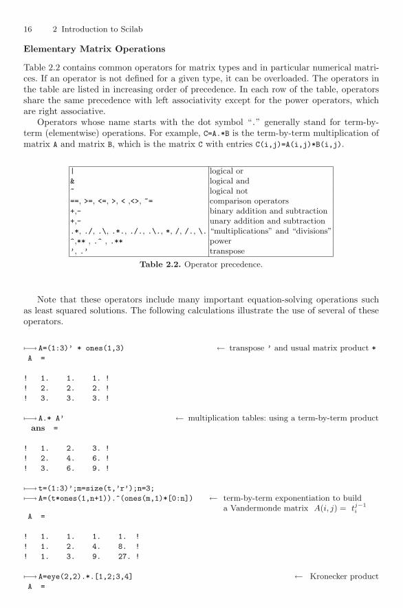
Elementary Matrix Operations
Table 2.2 contains common operators for matrix types and in particular numerical matri-ces. If an operator is not defined for a given type, it can be overloaded. The operators inthe table are listed in increasing order of precedence. In each row of the table, operatorsshare the same precedence with left associativity except for the power operators, whichare right associative.
Operators whose name starts with the dot symbol “.” generally stand for term-by-term (elementwise) operations. For example, C=A.*B is the term-by-term multiplication ofmatrix A and matrix B, which is the matrix C with entries C(i,j)=A(i,j)*B(i,j).
| logical or& logical and~ logical not==, >=, <=, >, < ,<>, ~= comparison operators+,- binary addition and subtraction+,- unary addition and subtraction.*, ./, .\, .*., ./., .\., *, /, /., \. “multiplications” and “divisions”^,** , .^ , .** power’, .’ transpose
Table 2.2. Operator precedence.
Note that these operators include many important equation-solving operations suchas least squared solutions. The following calculations illustrate the use of several of theseoperators.
�−→ A=(1:3)’ * ones(1,3) ← transpose ’ and usual matrix product *
A =
! 1. 1. 1. !
! 2. 2. 2. !
! 3. 3. 3. !
�−→ A.* A’ ← multiplication tables: using a term-by-term productans =
! 1. 2. 3. !
! 2. 4. 6. !
! 3. 6. 9. !
�−→ t=(1:3)’;m=size(t,’r’);n=3;
�−→ A=(t*ones(1,n+1)).^(ones(m,1)*[0:n]) ← term-by-term exponentiation to builda Vandermonde matrix A(i, j) = tj−1
iA =
! 1. 1. 1. 1. !
! 1. 2. 4. 8. !
! 1. 3. 9. 27. !
�−→ A=eye(2,2).*.[1,2;3,4] ← Kronecker productA =
2.1 Scilab Objects 17
! 1. 2. 0. 0. !
! 3. 4. 0. 0. !
! 0. 0. 1. 2. !
! 0. 0. 3. 4. !
�−→ A=[1,2;3,4];b=[5;6];
�−→ x = A \ b ; norm(A*x -b) ← \ for solving a linear system Ax=b.ans =
0.
�−→ A1=[A,zeros(A)]; x = A1 \ b ← underdetermined system: a solution withminimum norm is returned
x =
! - 4. !
! 4.5 !
! 0. !
! 0. !
�−→ A1=[A;A]; x = A1\ [b;7;8] ← overdetermined system: a least squaredsolution is returned
x =
! - 5. !
! 5.5 !
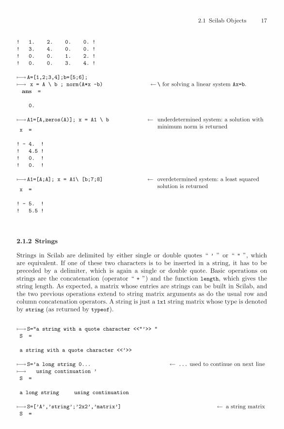
2.1.2 Strings
Strings in Scilab are delimited by either single or double quotes “ ’ ” or “ " ”, whichare equivalent. If one of these two characters is to be inserted in a string, it has to bepreceded by a delimiter, which is again a single or double quote. Basic operations onstrings are the concatenation (operator “ + ”) and the function length, which gives thestring length. As expected, a matrix whose entries are strings can be built in Scilab, andthe two previous operations extend to string matrix arguments as do the usual row andcolumn concatenation operators. A string is just a 1x1 string matrix whose type is denotedby string (as returned by typeof).
�−→ S="a string with a quote character <<"’>> "
S =
a string with a quote character <<’>>
�−→ S=’a long string 0... ← ... used to continue on next line�−→ using continuation ’
S =
a long string using continuation
�−→ S=[’A’,’string’;’2x2’,’matrix’] ← a string matrixS =

18 2 Introduction to Scilab
!A string !
! !
!2x2 matrix !
�−→ length(S) ← length of each string of S in a matrixans =
! 1. 6. !
! 3. 6. !
ascii conversion from string to ascii valuesexecstr send a string to the Scilab interpretergrep search for occurences of a string in a string matrixpart substring extractionmsscanf scans input from a string according to a formatmsprintf builds a string by output according to a formatstrindex finds occurrences of strings in a stringstring converts data to stringstripblanks remove leading and trailing white (blank) charactersstrsubst string substitution in a string matrixtokens string tokenizerstrcat concatenate string matrix entrieslength length of string matrix entries
Table 2.3. Some string matrix functions.
String matrix utility functions are listed in Table 2.3. The next session shows how someof them can be used.
�−→ A=rand(2,8,’n’); ← Normal law�−→ A=sign(A); ← just keep the signs�−→ A=string(A) ← convert to string matrixA =
!-1 1 1 1 1 1 -1 1 !
! !
!1 1 1 1 -1 -1 -1 1 !
�−→ A=strsubst(A,’1’,’+’); ← string substitution�−→ A=strsubst(A,’-+’,’-’) ← string substitutionA =
!- + + + + + - + !
! !
!+ + + + - - - + !
The command execstr can be used to evaluate a string as a Scilab expression. Thegiven string is evaluated using values from the current context. Thus, string matrices
2.1 Scilab Objects 19
can be used to build Scilab expressions, which then can be evaluated as if they wereentered interactively in Scilab. An important extra argument ’errcatch’ can be given tothe execstr function in order to supress the Scilab standard error mechanism while thestring is evaluated.
�−→ name =’x’; n=3; val=[45,67,34];
�−→ str = name +string(1:n)+’=val(’ +string(1:n)+’);’ ← a string vectorstr =
!x1=val(1); x2=val(2); x3=val(3); !
�−→ execstr(str); ← Scilab evaluation of str�−→ [x1,x2,x3] ← x1, x2 and x3 are now defined
ans =
! 45. 67. 34. !
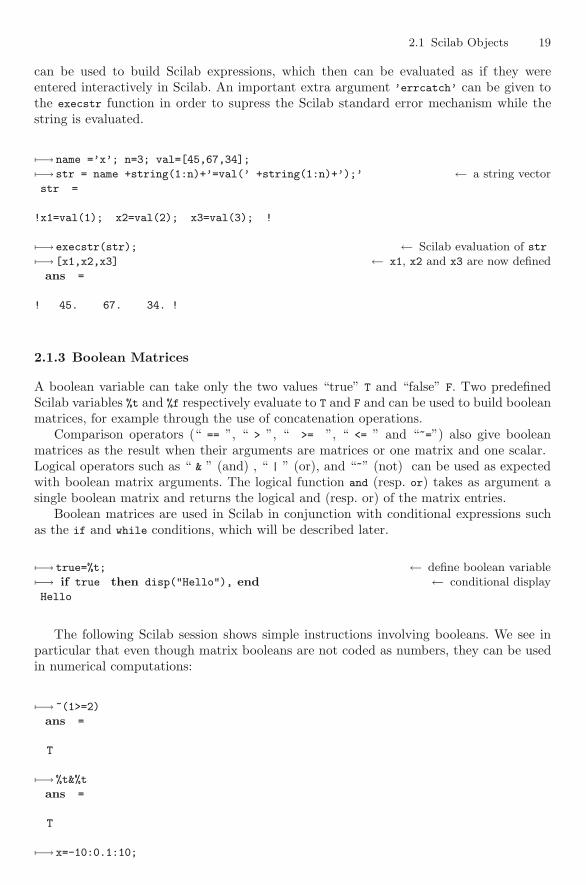
2.1.3 Boolean Matrices
A boolean variable can take only the two values “true” T and “false” F. Two predefinedScilab variables %t and %f respectively evaluate to T and F and can be used to build booleanmatrices, for example through the use of concatenation operations.
Comparison operators (“ == ”, “ > ”, “ >= ”, “ <= ” and “~=”) also give booleanmatrices as the result when their arguments are matrices or one matrix and one scalar.Logical operators such as “ & ” (and) , “ | ” (or), and “~” (not) can be used as expectedwith boolean matrix arguments. The logical function and (resp. or) takes as argument asingle boolean matrix and returns the logical and (resp. or) of the matrix entries.
Boolean matrices are used in Scilab in conjunction with conditional expressions suchas the if and while conditions, which will be described later.
�−→ true=%t; ← define boolean variable�−→ if true then disp("Hello"), end ← conditional displayHello
The following Scilab session shows simple instructions involving booleans. We see inparticular that even though matrix booleans are not coded as numbers, they can be usedin numerical computations:
�−→ ~(1>=2)
ans =
T
�−→ %t&%t
ans =
T
�−→ x=-10:0.1:10;
20 2 Introduction to Scilab
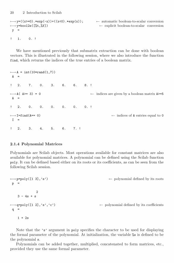
�−→ y=((x>=0).*exp(-x))+((x<0).*exp(x)); ← automatic boolean-to-scalar conversion�−→ y=bool2s([%t,%f]) ← explicit boolean-to-scalar conversiony =
! 1. 0. !
We have mentioned previously that submatrix extraction can be done with booleanvectors. This is illustrated in the following session, where we also introduce the functionfind, which returns the indices of the true entries of a boolean matrix.
�−→ A = int(10*rand(1,7))
A =
! 2. 7. 0. 3. 6. 6. 8. !
�−→ A( A>= 3) = 0 ← indices are given by a boolean matrix A>=5
A =
! 2. 0. 0. 0. 0. 0. 0. !
�−→ I=find(A== 0) ← indices of A entries equal to 0
I =
! 2. 3. 4. 5. 6. 7. !
2.1.4 Polynomial Matrices
Polynomials are Scilab objects. Most operations available for constant matrices are alsoavailable for polynomial matrices. A polynomial can be defined using the Scilab functionpoly. It can be defined based either on its roots or its coefficients, as can be seen from thefollowing Scilab session.
�−→ p=poly([1 3],’s’) ← polynomial defined by its rootsp =
2
3 - 4s + s
�−→ q=poly([1 2],’s’,’c’) ← polynomial defined by its coefficientsq =
1 + 2s
Note that the ’s’ argument in poly specifies the character to be used for displayingthe formal parameter of the polynomial. At initialization, the variable %s is defined to bethe polynomial s.
Polynomials can be added together, multiplied, concatenated to form matrices, etc.,provided they use the same formal parameter.
2.1 Scilab Objects 21
�−→ p+q+1 ← polynomial/constant additionans =
2
5 - 2s + s
�−→ [p*q,1] ← matrix polynomialans =
! 2 3 !
! 3 + 2s - 7s + 2s 1 !
A polynomial can even be divided by a polynomial, and a polynomial matrix inverted,but the result, in general, is not a polynomial. It is a rational function, which is anotherScilab object constructed using a list object, as we shall see later.
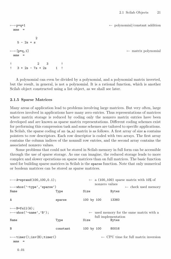
2.1.5 Sparse Matrices
Many areas of application lead to problems involving large matrices. But very often, largematrices involved in applications have many zero entries. Thus representations of matriceswhere matrix storage is reduced by coding only the nonzero matrix entries have beendeveloped and are known as sparse matrix representations. Different coding schemes existfor performing this compression task and some schemes are tailored to specific applications.In Scilab, the sparse coding of an (m,n) matrix is as follows. A first array of size m containspointers to row descriptors. Each row descriptor is coded with two arrays. The first arraycontains the column indices of the nonnull row entries, and the second array contains theassociated nonzero values.
Some problems that could not be stored in Scilab memory in full form can be accessiblethrough the use of sparse storage. As one can imagine, the reduced storage leads to morecomplex and slower operations on sparse matrices than on full matrices. The basic functionused for building sparse matrices in Scilab is the sparse function. Note that only numericalor boolean matrices can be stored as sparse matrices.
�−→ A=sprand(100,100,0.1); ← a (100,100) sparse matrix with 10% ofnonzero values�−→ whos(’-type’,’sparse’) ← check used memory
Name Type Size Bytes
A sparse 100 by 100 13360
�−→ B=full(A);
�−→ whos(’-name’,’B’); ← used memory for the same matrix with afull implementation
Name Type Size Bytes
B constant 100 by 100 80016
�−→ timer();inv(B);timer() ← CPU time for full matrix inversionans =
0.01

22 2 Introduction to Scilab
�−→ timer();inv(A);timer() ← CPU time for sparse matrix inversionans =
0.28
While useful in illustrating the commands, this example was only 100 × 100, which isnot considered today to be a very large matrix. Also, this matrix was random, and manysparse matrices, such as those that arise by the discretization of PDEs, are not random.They have stronger structural properties that can be exploited.
2.1.6 Lists
Scilab lists are built with the list, tlist, and mlist functions. These three functions donot exactly build lists, but they can be considered to be structure builders in the sense thatthey are used to aggregate under a unique variable name a set of objects of different types.They are implemented as an array of variable-size objects that is not a list implementation.A type corresponds to each builder function, and they are recursive types (a list elementcan be a list).
• If the list constructor is used, then the stored objects are accessed by an index givingtheir position in the list.
• If the tlist constructor is used, then the built object has a new dynamic type andstored objects can be accessed through names. Note also that the fields are dynamic,which means that new fields can be dynamically added or removed from an occurrenceof a tlist. A tlist remains a list, and access to stored objects through indices is alsopossible.
• The mlist constructor is a slight variation of the tlist constructor. The only differenceis that the predefined access to stored objects through indices is no longer effective (itis, however, possible using the getfield and setfield functions). Also, extraction andinsertion operators can be overloaded for mlist objects. This means that it is possibleto give a meaning to multi-indices extraction or insertion operations. hypermat objectsthat implement multidimensional arrays are implemented using mlist in Scilab.
Note that many Scilab objects are implemented as tlist and mlist, and from theuser point of view this is not important. For example, suppose that you want to define avariable with an extendable number of fields. This is done very easily through the use ofthe “.” operator:
�−→ x.color = 4;
�−→ x.value = rand(1,3);
�−→ x.name = ’foo’;
�−→ x ← x is a tlist of type struct (st)ans =
color: 4
value: [0.2113249,0.7560439,0.0002211]
name: "foo"

2.1 Scilab Objects 23
Among Scilab objects coded this way, it is important to mention the rational matricesand the linear state-space systems, which play important roles in modeling and analysisof linear systems.
The following session illustrates the use of rational matrices in Scilab (recall that %s isby default the polynomial s). Note that all the elementary operations are overloaded forrational matrices.
�−→ r=1/%s ← defining a rational numberr =
1
-
s
�−→ a=[1,r;1,1] ← rational matrix constructiona =
! 1 1 !
! - - !
! 1 s !
! !
! 1 1 !
! - - !
! 1 1 !
�−→ b=inv(a) ← matrix inversionb =
! s - 1 !
! ----- ----- !
! - 1 + s - 1 + s !
! !
! - s s !
! ----- ----- !
! - 1 + s - 1 + s !
�−→ b.num ← numerator fieldans =
! s - 1 !
! !
! - s s !
�−→ b.den ← denominator fieldans =
! - 1 + s - 1 + s !
! !
! - 1 + s - 1 + s !
A linear state-space system is characterized in terms of four matrices, A, B, C, andD; we will describe and use these systems later for modeling linear systems. The Scilabfunction ssrand defines a random system with given input, output, and state sizes.

24 2 Introduction to Scilab
�−→ sys=ssrand(1,1,2) ← defines a linear systemsys =
sys(1) (state-space system:)
!lss A B C D X0 dt !
sys(2) = A matrix =
! - 0.7616491 1.4739762 !
! 0.6755537 1.1443051 !
sys(3) = B matrix =
! 0.8529775 !
! 0.4529708 !
sys(4) = C matrix =
! 0.7223316 1.9273333 !
sys(5) = D matrix =
0.
sys(6) = X0 (initial state) =
! 0. !
! 0. !
sys(7) = Time domain =
c
�−→ sys.A ← extract the A matrixans =
! - 0.7616491 1.4739762 !
! 0.6755537 1.1443051 !
Common operations on lists are illustrated in the following example. Note that onecan define an entry starting somewhere other than entry 1, but then the list will createearly places for entries. This is analogous to Scilab automatically setting up a 3×5 matrixwhen the instruction A(3,5)=6.7 is entered. Except now, instead of extra zero entries, anentry called Undefined fills out the earlier positions in the list.
�−→ L=list() ← an empty listL =
()
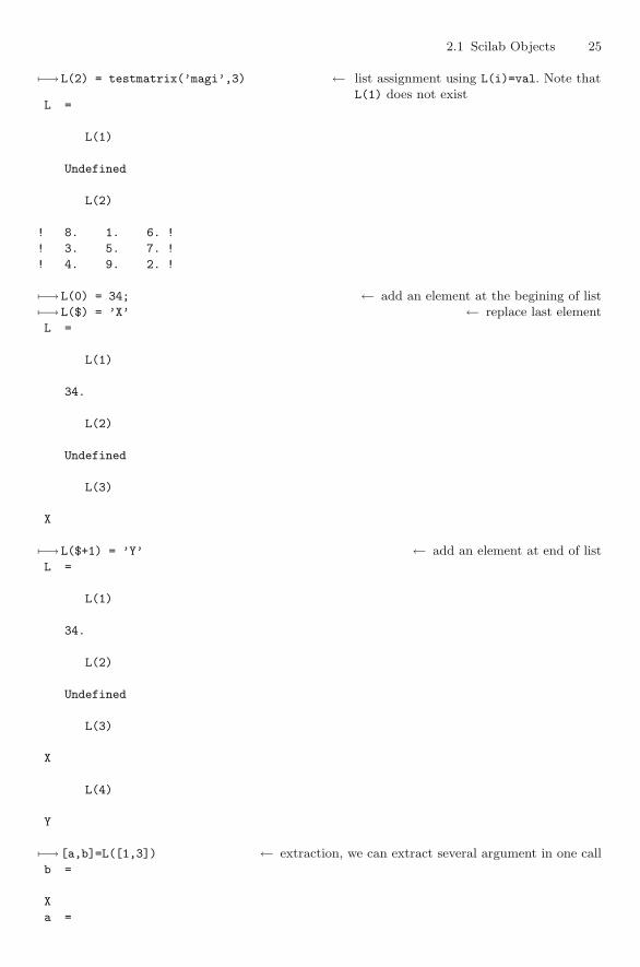
2.1 Scilab Objects 25
�−→ L(2) = testmatrix(’magi’,3) ← list assignment using L(i)=val. Note thatL(1) does not exist
L =
L(1)
Undefined
L(2)
! 8. 1. 6. !
! 3. 5. 7. !
! 4. 9. 2. !
�−→ L(0) = 34; ← add an element at the begining of list�−→ L($) = ’X’ ← replace last elementL =
L(1)
34.
L(2)
Undefined
L(3)
X
�−→ L($+1) = ’Y’ ← add an element at end of listL =
L(1)
34.
L(2)
Undefined
L(3)
X
L(4)
Y
�−→ [a,b]=L([1,3]) ← extraction, we can extract several argument in one callb =
X
a =
26 2 Introduction to Scilab
34.
�−→ L(2)=null(); ← deletion of the second list element
2.1.7 Functions
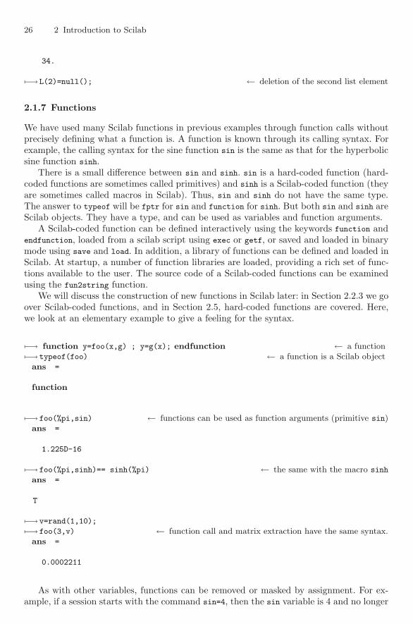
We have used many Scilab functions in previous examples through function calls withoutprecisely defining what a function is. A function is known through its calling syntax. Forexample, the calling syntax for the sine function sin is the same as that for the hyperbolicsine function sinh.
There is a small difference between sin and sinh. sin is a hard-coded function (hard-coded functions are sometimes called primitives) and sinh is a Scilab-coded function (theyare sometimes called macros in Scilab). Thus, sin and sinh do not have the same type.The answer to typeof will be fptr for sin and function for sinh. But both sin and sinh areScilab objects. They have a type, and can be used as variables and function arguments.
A Scilab-coded function can be defined interactively using the keywords function andendfunction, loaded from a scilab script using exec or getf, or saved and loaded in binarymode using save and load. In addition, a library of functions can be defined and loaded inScilab. At startup, a number of function libraries are loaded, providing a rich set of func-tions available to the user. The source code of a Scilab-coded functions can be examinedusing the fun2string function.
We will discuss the construction of new functions in Scilab later: in Section 2.2.3 we goover Scilab-coded functions, and in Section 2.5, hard-coded functions are covered. Here,we look at an elementary example to give a feeling for the syntax.
�−→ function y=foo(x,g) ; y=g(x); endfunction ← a function�−→ typeof(foo) ← a function is a Scilab object
ans =
function
�−→ foo(%pi,sin) ← functions can be used as function arguments (primitive sin)ans =
1.225D-16
�−→ foo(%pi,sinh)== sinh(%pi) ← the same with the macro sinh
ans =
T
�−→ v=rand(1,10);
�−→ foo(3,v) ← function call and matrix extraction have the same syntax.ans =
0.0002211
As with other variables, functions can be removed or masked by assignment. For ex-ample, if a session starts with the command sin=4, then the sin variable is 4 and no longer
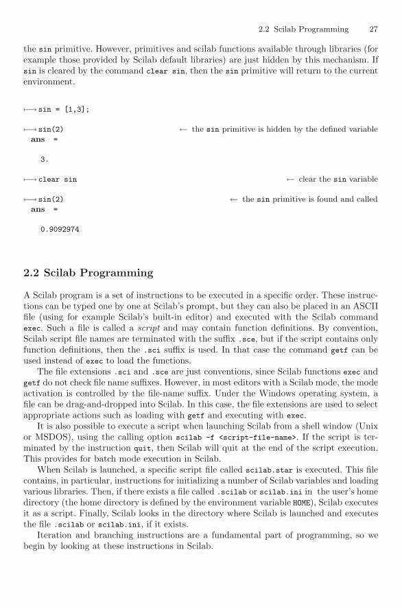
2.2 Scilab Programming 27
the sin primitive. However, primitives and scilab functions available through libraries (forexample those provided by Scilab default libraries) are just hidden by this mechanism. Ifsin is cleared by the command clear sin, then the sin primitive will return to the currentenvironment.
�−→ sin = [1,3];
�−→ sin(2) ← the sin primitive is hidden by the defined variableans =
3.
�−→ clear sin ← clear the sin variable
�−→ sin(2) ← the sin primitive is found and calledans =
0.9092974
2.2 Scilab Programming
A Scilab program is a set of instructions to be executed in a specific order. These instruc-tions can be typed one by one at Scilab’s prompt, but they can also be placed in an ASCIIfile (using for example Scilab’s built-in editor) and executed with the Scilab commandexec. Such a file is called a script and may contain function definitions. By convention,Scilab script file names are terminated with the suffix .sce, but if the script contains onlyfunction definitions, then the .sci suffix is used. In that case the command getf can beused instead of exec to load the functions.
The file extensions .sci and .sce are just conventions, since Scilab functions exec andgetf do not check file name suffixes. However, in most editors with a Scilab mode, the modeactivation is controlled by the file-name suffix. Under the Windows operating system, afile can be drag-and-dropped into Scilab. In this case, the file extensions are used to selectappropriate actions such as loading with getf and executing with exec.
It is also possible to execute a script when launching Scilab from a shell window (Unixor MSDOS), using the calling option scilab -f <script-file-name>. If the script is ter-minated by the instruction quit, then Scilab will quit at the end of the script execution.This provides for batch mode execution in Scilab.
When Scilab is launched, a specific script file called scilab.star is executed. This filecontains, in particular, instructions for initializing a number of Scilab variables and loadingvarious libraries. Then, if there exists a file called .scilab or scilab.ini in the user’s homedirectory (the home directory is defined by the environment variable HOME), Scilab executesit as a script. Finally, Scilab looks in the directory where Scilab is launched and executesthe file .scilab or scilab.ini, if it exists.
Iteration and branching instructions are a fundamental part of programming, so webegin by looking at these instructions in Scilab.
28 2 Introduction to Scilab
2.2.1 Branching
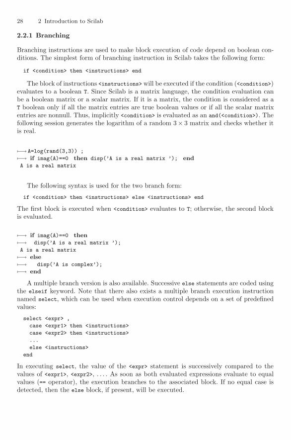
Branching instructions are used to make block execution of code depend on boolean con-ditions. The simplest form of branching instruction in Scilab takes the following form:
if <condition> then <instructions> end
The block of instructions <instructions> will be executed if the condition (<condition>)evaluates to a boolean T. Since Scilab is a matrix language, the condition evaluation canbe a boolean matrix or a scalar matrix. If it is a matrix, the condition is considered as aT boolean only if all the matrix entries are true boolean values or if all the scalar matrixentries are nonnull. Thus, implicitly <condition> is evaluated as an and(<condition>). Thefollowing session generates the logarithm of a random 3× 3 matrix and checks whether itis real.
�−→ A=log(rand(3,3)) ;
�−→ if imag(A)==0 then disp(’A is a real matrix ’); endA is a real matrix
The following syntax is used for the two branch form:
if <condition> then <instructions> else <instructions> end
The first block is executed when <condition> evaluates to T; otherwise, the second blockis evaluated.
�−→ if imag(A)==0 then�−→ disp(’A is a real matrix ’);
A is a real matrix
�−→ else�−→ disp(’A is complex’);
�−→ end
A multiple branch version is also available. Successive else statements are coded usingthe elseif keyword. Note that there also exists a multiple branch execution instructionnamed select, which can be used when execution control depends on a set of predefinedvalues:
select <expr> ,
case <expr1> then <instructions>
case <expr2> then <instructions>
...
else <instructions>
end
In executing select, the value of the <expr> statement is successively compared to thevalues of <expr1>, <expr2>, . . . . As soon as both evaluated expressions evaluate to equalvalues (== operator), the execution branches to the associated block. If no equal case isdetected, then the else block, if present, will be executed.
2.2 Scilab Programming 29
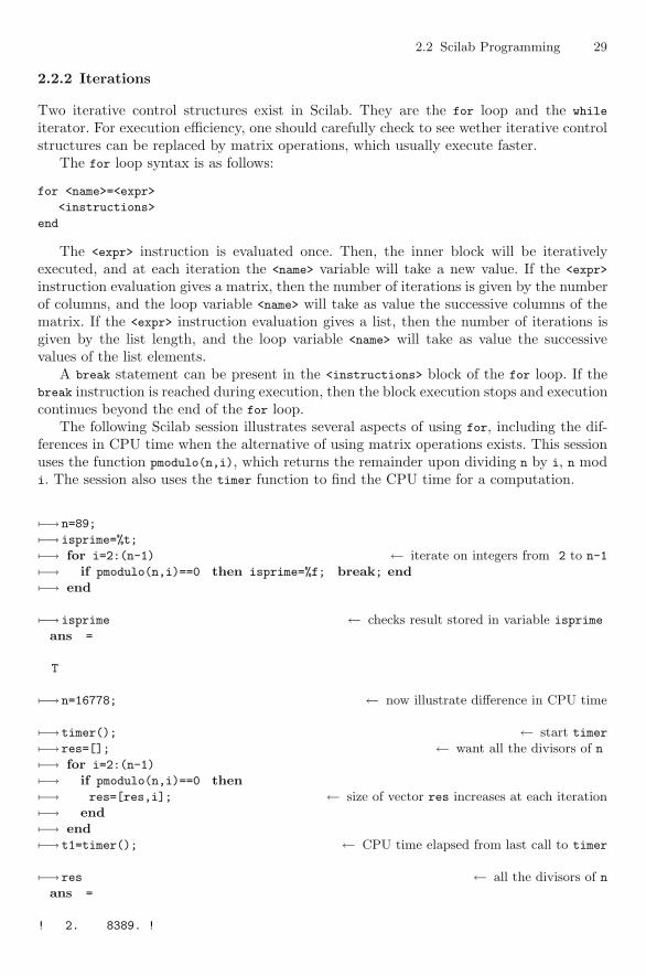
2.2.2 Iterations
Two iterative control structures exist in Scilab. They are the for loop and the while
iterator. For execution efficiency, one should carefully check to see wether iterative controlstructures can be replaced by matrix operations, which usually execute faster.
The for loop syntax is as follows:
for <name>=<expr>
<instructions>
end
The <expr> instruction is evaluated once. Then, the inner block will be iterativelyexecuted, and at each iteration the <name> variable will take a new value. If the <expr>
instruction evaluation gives a matrix, then the number of iterations is given by the numberof columns, and the loop variable <name> will take as value the successive columns of thematrix. If the <expr> instruction evaluation gives a list, then the number of iterations isgiven by the list length, and the loop variable <name> will take as value the successivevalues of the list elements.
A break statement can be present in the <instructions> block of the for loop. If thebreak instruction is reached during execution, then the block execution stops and executioncontinues beyond the end of the for loop.
The following Scilab session illustrates several aspects of using for, including the dif-ferences in CPU time when the alternative of using matrix operations exists. This sessionuses the function pmodulo(n,i), which returns the remainder upon dividing n by i, n modi. The session also uses the timer function to find the CPU time for a computation.
�−→ n=89;
�−→ isprime=%t;
�−→ for i=2:(n-1) ← iterate on integers from 2 to n-1
�−→ if pmodulo(n,i)==0 then isprime=%f; break; end�−→ end
�−→ isprime ← checks result stored in variable isprime
ans =
T
�−→ n=16778; ← now illustrate difference in CPU time
�−→ timer(); ← start timer
�−→ res=[]; ← want all the divisors of n�−→ for i=2:(n-1)
�−→ if pmodulo(n,i)==0 then�−→ res=[res,i]; ← size of vector res increases at each iteration�−→ end�−→ end�−→ t1=timer(); ← CPU time elapsed from last call to timer
�−→ res ← all the divisors of nans =
! 2. 8389. !
30 2 Introduction to Scilab
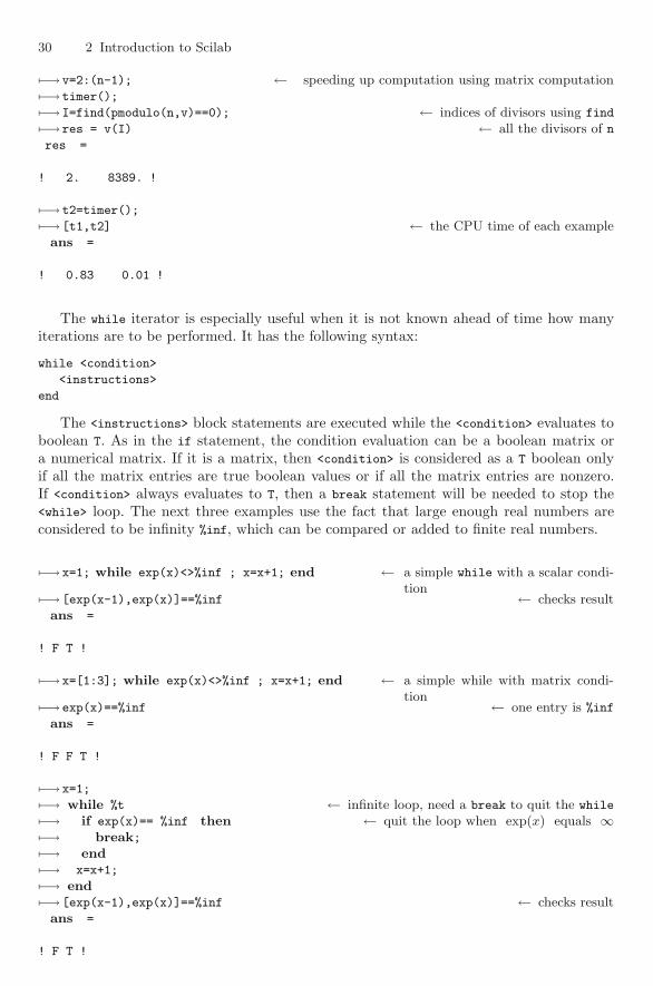
�−→ v=2:(n-1); ← speeding up computation using matrix computation�−→ timer();
�−→ I=find(pmodulo(n,v)==0); ← indices of divisors using find
�−→ res = v(I) ← all the divisors of nres =
! 2. 8389. !
�−→ t2=timer();
�−→ [t1,t2] ← the CPU time of each exampleans =
! 0.83 0.01 !
The while iterator is especially useful when it is not known ahead of time how manyiterations are to be performed. It has the following syntax:
while <condition>
<instructions>
end
The <instructions> block statements are executed while the <condition> evaluates toboolean T. As in the if statement, the condition evaluation can be a boolean matrix ora numerical matrix. If it is a matrix, then <condition> is considered as a T boolean onlyif all the matrix entries are true boolean values or if all the matrix entries are nonzero.If <condition> always evaluates to T, then a break statement will be needed to stop the<while> loop. The next three examples use the fact that large enough real numbers areconsidered to be infinity %inf, which can be compared or added to finite real numbers.
�−→ x=1; while exp(x)<>%inf ; x=x+1; end ← a simple while with a scalar condi-tion�−→ [exp(x-1),exp(x)]==%inf ← checks result
ans =
! F T !
�−→ x=[1:3]; while exp(x)<>%inf ; x=x+1; end ← a simple while with matrix condi-tion�−→ exp(x)==%inf ← one entry is %inf
ans =
! F F T !
�−→ x=1;
�−→ while %t ← infinite loop, need a break to quit the while
�−→ if exp(x)== %inf then ← quit the loop when exp(x) equals ∞�−→ break;�−→ end�−→ x=x+1;
�−→ end�−→ [exp(x-1),exp(x)]==%inf ← checks result
ans =
! F T !
2.2 Scilab Programming 31
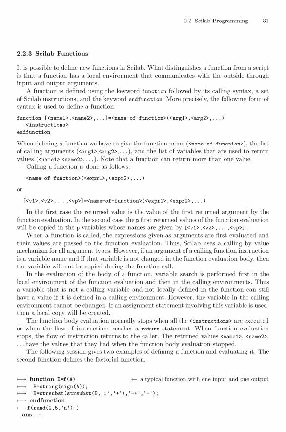
2.2.3 Scilab Functions
It is possible to define new functions in Scilab. What distinguishes a function from a scriptis that a function has a local environment that communicates with the outside throughinput and output arguments.
A function is defined using the keyword function followed by its calling syntax, a setof Scilab instructions, and the keyword endfunction. More precisely, the following form ofsyntax is used to define a function:
function [<name1>,<name2>,...]=<name-of-function>(<arg1>,<arg2>,...)
<instructions>
endfunction
When defining a function we have to give the function name (<name-of-function>), the listof calling arguments (<arg1>,<arg2>,...), and the list of variables that are used to returnvalues (<name1>,<name2>,...). Note that a function can return more than one value.
Calling a function is done as follows:
<name-of-function>(<expr1>,<expr2>,...)
or
[<v1>,<v2>,...,<vp>]=<name-of-function>(<expr1>,<expr2>,...)
In the first case the returned value is the value of the first returned argument by thefunction evaluation. In the second case the p first returned values of the function evaluationwill be copied in the p variables whose names are given by [<v1>,<v2>,...,<vp>].
When a function is called, the expressions given as arguments are first evaluated andtheir values are passed to the function evaluation. Thus, Scilab uses a calling by valuemechanism for all argument types. However, if an argument of a calling function instructionis a variable name and if that variable is not changed in the function evaluation body, thenthe variable will not be copied during the function call.
In the evaluation of the body of a function, variable search is performed first in thelocal environment of the function evaluation and then in the calling environments. Thusa variable that is not a calling variable and not locally defined in the function can stillhave a value if it is defined in a calling environment. However, the variable in the callingenvironment cannot be changed. If an assignment statement involving this variable is used,then a local copy will be created.
The function body evaluation normally stops when all the <instructions> are executedor when the flow of instructions reaches a return statement. When function evaluationstops, the flow of instruction returns to the caller. The returned values <name1>, <name2>,. . . have the values that they had when the function body evaluation stopped.
The following session gives two examples of defining a function and evaluating it. Thesecond function defines the factorial function.
�−→ function B=f(A) ← a typical function with one input and one output�−→ B=string(sign(A));
�−→ B=strsubst(strsubst(B,’1’,’+’),’-+’,’-’);
�−→ endfunction�−→ f(rand(2,5,’n’) )
ans =

32 2 Introduction to Scilab
!- + + + + !
! !
!+ + + + - !
�−→ function y=fact(x) ← a recursive function can be defined: fact calls fact
�−→ if x <= 1 then y=x; else y=x*fact(x-1); end�−→ endfunction
�−→ fact(4)
ans =
24.
This next script defines several functions and illustrates the rules for searching variablevalues when a function is evaluated. This is important but quite technical and can beomitted for first-time readers.
�−→ function y=f(x); y=2*x; endfunction
�−→ x=90;
�−→ f() ← argument x is not given but exists in thecalling environment. Thus, the calling se-quence works
ans =
180.
�−→ f(5,7) ← error: two many given arguments!--error 58
incorrect number of arguments in function call...
arguments are :
x
�−→ [a,b]=f(5) ← error: asking for too many returned arguments!--error 59
incorrect # of outputs in the functionarguments are :
y
�−→ function y=f(x); z=x; endfunction ← a new definition of f
�−→ y=89;
�−→ z=67;
�−→ w=f(x) ← y is not computed inside f but it has avalue in the calling environment. This isthe returned value
w =
89.
�−→ z ← z was not modified by execution of f
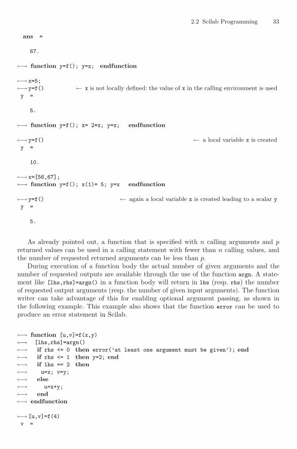
2.2 Scilab Programming 33
ans =
67.
�−→ function y=f(); y=x; endfunction
�−→ x=5;
�−→ y=f() ← x is not locally defined: the value of x in the calling environment is usedy =
5.
�−→ function y=f(); x= 2*x; y=x; endfunction
�−→ y=f() ← a local variable x is createdy =
10.
�−→ x=[56,67];
�−→ function y=f(); x(1)= 5; y=x endfunction
�−→ y=f() ← again a local variable x is created leading to a scalar y
y =
5.
As already pointed out, a function that is specified with n calling arguments and preturned values can be used in a calling statement with fewer than n calling values, andthe number of requested returned arguments can be less than p.
During execution of a function body the actual number of given arguments and thenumber of requested outputs are available through the use of the function argn. A state-ment like [lhs,rhs]=argn() in a function body will return in lhs (resp. rhs) the numberof requested output arguments (resp. the number of given input arguments). The functionwriter can take advantage of this for enabling optional argument passing, as shown inthe following example. This example also shows that the function error can be used toproduce an error statement in Scilab.
�−→ function [u,v]=f(x,y)
�−→ [lhs,rhs]=argn()
�−→ if rhs <= 0 then error(’at least one argument must be given’); end�−→ if rhs <= 1 then y=2; end�−→ if lhs == 2 then�−→ u=x; v=y;
�−→ else�−→ u=x+y;
�−→ end�−→ endfunction
�−→ [u,v]=f(4)
v =
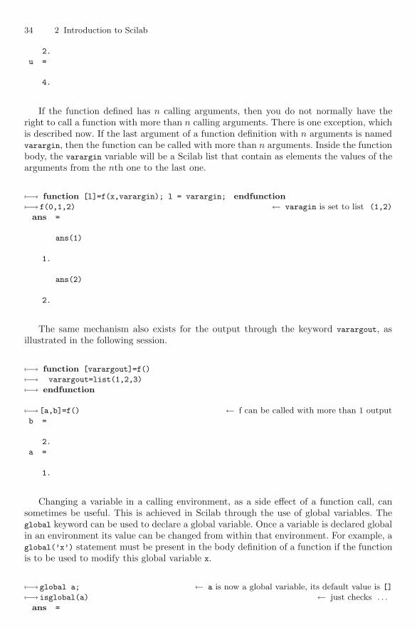
34 2 Introduction to Scilab
2.
u =
4.
If the function defined has n calling arguments, then you do not normally have theright to call a function with more than n calling arguments. There is one exception, whichis described now. If the last argument of a function definition with n arguments is namedvarargin, then the function can be called with more than n arguments. Inside the functionbody, the varargin variable will be a Scilab list that contain as elements the values of thearguments from the nth one to the last one.
�−→ function [l]=f(x,varargin); l = varargin; endfunction�−→ f(0,1,2) ← varagin is set to list (1,2)
ans =
ans(1)
1.
ans(2)
2.
The same mechanism also exists for the output through the keyword varargout, asillustrated in the following session.
�−→ function [varargout]=f()
�−→ varargout=list(1,2,3)
�−→ endfunction
�−→ [a,b]=f() ← f can be called with more than 1 outputb =
2.
a =
1.
Changing a variable in a calling environment, as a side effect of a function call, cansometimes be useful. This is achieved in Scilab through the use of global variables. Theglobal keyword can be used to declare a global variable. Once a variable is declared globalin an environment its value can be changed from within that environment. For example, aglobal(’x’) statement must be present in the body definition of a function if the functionis to be used to modify this global variable x.
�−→ global a; ← a is now a global variable, its default value is []
�−→ isglobal(a) ← just checks . . .ans =
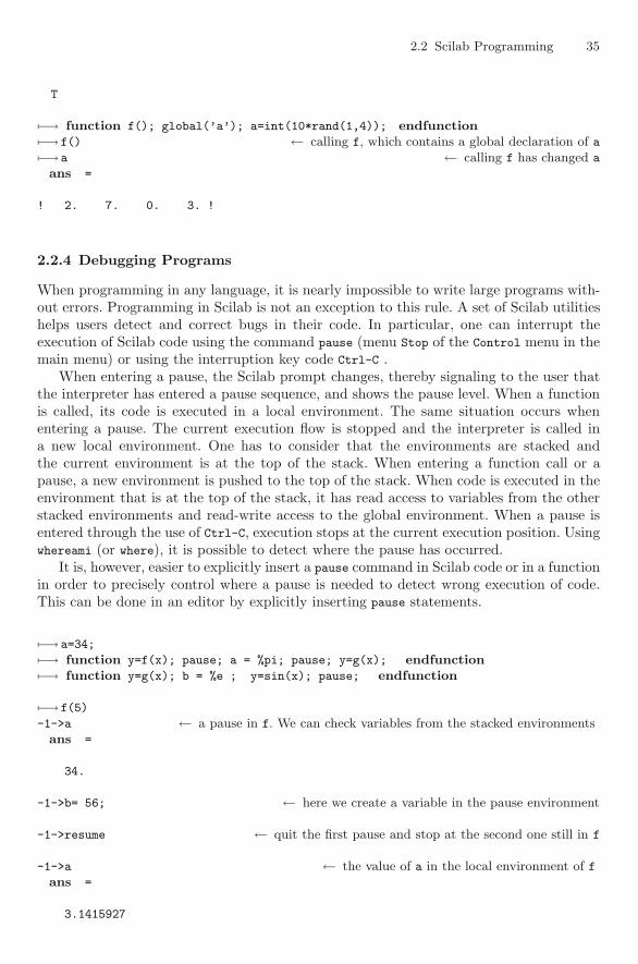
2.2 Scilab Programming 35
T
�−→ function f(); global(’a’); a=int(10*rand(1,4)); endfunction�−→ f() ← calling f, which contains a global declaration of a�−→ a ← calling f has changed a
ans =
! 2. 7. 0. 3. !
2.2.4 Debugging Programs
When programming in any language, it is nearly impossible to write large programs with-out errors. Programming in Scilab is not an exception to this rule. A set of Scilab utilitieshelps users detect and correct bugs in their code. In particular, one can interrupt theexecution of Scilab code using the command pause (menu Stop of the Control menu in themain menu) or using the interruption key code Ctrl-C .
When entering a pause, the Scilab prompt changes, thereby signaling to the user thatthe interpreter has entered a pause sequence, and shows the pause level. When a functionis called, its code is executed in a local environment. The same situation occurs whenentering a pause. The current execution flow is stopped and the interpreter is called ina new local environment. One has to consider that the environments are stacked andthe current environment is at the top of the stack. When entering a function call or apause, a new environment is pushed to the top of the stack. When code is executed in theenvironment that is at the top of the stack, it has read access to variables from the otherstacked environments and read-write access to the global environment. When a pause isentered through the use of Ctrl-C, execution stops at the current execution position. Usingwhereami (or where), it is possible to detect where the pause has occurred.
It is, however, easier to explicitly insert a pause command in Scilab code or in a functionin order to precisely control where a pause is needed to detect wrong execution of code.This can be done in an editor by explicitly inserting pause statements.
�−→ a=34;
�−→ function y=f(x); pause; a = %pi; pause; y=g(x); endfunction�−→ function y=g(x); b = %e ; y=sin(x); pause; endfunction
�−→ f(5)
-1->a ← a pause in f. We can check variables from the stacked environmentsans =
34.
-1->b= 56; ← here we create a variable in the pause environment
-1->resume ← quit the first pause and stop at the second one still in f
-1->a ← the value of a in the local environment of fans =
3.1415927
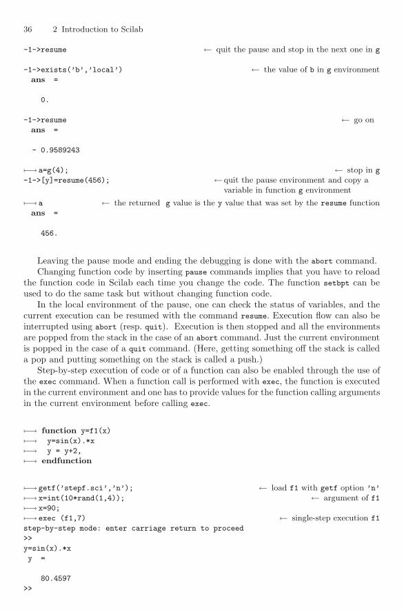
36 2 Introduction to Scilab
-1->resume ← quit the pause and stop in the next one in g
-1->exists(’b’,’local’) ← the value of b in g environmentans =
0.
-1->resume ← go onans =
- 0.9589243
�−→ a=g(4); ← stop in g
-1->[y]=resume(456); ← quit the pause environment and copy avariable in function g environment
�−→ a ← the returned g value is the y value that was set by the resume functionans =
456.
Leaving the pause mode and ending the debugging is done with the abort command.Changing function code by inserting pause commands implies that you have to reload
the function code in Scilab each time you change the code. The function setbpt can beused to do the same task but without changing function code.
In the local environment of the pause, one can check the status of variables, and thecurrent execution can be resumed with the command resume. Execution flow can also beinterrupted using abort (resp. quit). Execution is then stopped and all the environmentsare popped from the stack in the case of an abort command. Just the current environmentis popped in the case of a quit command. (Here, getting something off the stack is calleda pop and putting something on the stack is called a push.)
Step-by-step execution of code or of a function can also be enabled through the use ofthe exec command. When a function call is performed with exec, the function is executedin the current environment and one has to provide values for the function calling argumentsin the current environment before calling exec.
�−→ function y=f1(x)
�−→ y=sin(x).*x
�−→ y = y+2,
�−→ endfunction
�−→ getf(’stepf.sci’,’n’); ← load f1 with getf option ’n’
�−→ x=int(10*rand(1,4)); ← argument of f1�−→ x=90;
�−→ exec (f1,7) ← single-step execution f1
step-by-step mode: enter carriage return to proceed
>>
y=sin(x).*x
y =
80.4597
>>
2.3 Input and Output Functions 37
y = y+2,
y =
82.4597
>>
return!
Note that by default, the source code of the function instructions is hidden when getf
is used. In order to see the source code, one has to load the function into the Scilabenvironment with the getf command associated with the optional argument ’n’.
Finally, it should be noted that the built-in editor also provides some debugging facil-ities.
2.3 Input and Output Functions
The default for Scilab commands is to show the results in the command window unlessthey create a graphic, and then the default is to show the result in a graphics window.However, it is often desired to have the result saved in a file or printed on a printer. Inthis section we discuss how to control the input and output of different types of data.
2.3.1 Display of Variables
As already seen in previous examples, when a Scilab instruction is followed by a commaor a line feed, a display of the instruction evaluation result is provided. If instructions areended by a semicolon or belong to the body of a function, then no display occurs.
Sometimes one wants values of variables inside of functions to be displayed or output toa file. Explicit display of the value of a variable, or of the result of an instruction evaluation,is achieved by the function disp or print. These two functions provide a display similar tothe one obtained automatically in the command window. The first argument of the print
function is used to control the output stream (disp uses the Scilab command windowas output stream). One can use a file name given by a Scilab string or a file descriptor(returned by the file command). Alternatively one can use the predefined value %io(2),which stands for the standard output stream in the Scilab command window.
�−→ a=[%pi,4,%inf] ← the result is displayeda =
! 3.1415927 4. Inf !
�−→ print(%io(2),a) ← using print to display a variable (same as disp)a =
! 3.1415927 4. Inf !
�−→ print(’a.txt’,a) ← print to file a.txt
print can be used to force the display of variables inside a function during its execution,as illustrated below:
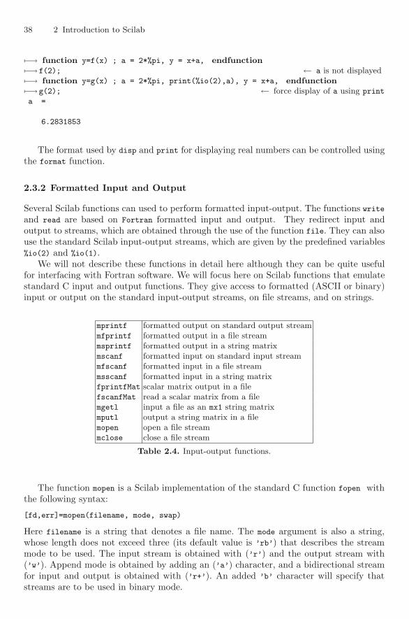
38 2 Introduction to Scilab
�−→ function y=f(x) ; a = 2*%pi, y = x+a, endfunction�−→ f(2); ← a is not displayed�−→ function y=g(x) ; a = 2*%pi, print(%io(2),a), y = x+a, endfunction�−→ g(2); ← force display of a using print
a =
6.2831853
The format used by disp and print for displaying real numbers can be controlled usingthe format function.
2.3.2 Formatted Input and Output
Several Scilab functions can used to perform formatted input-output. The functions writeand read are based on Fortran formatted input and output. They redirect input andoutput to streams, which are obtained through the use of the function file. They can alsouse the standard Scilab input-output streams, which are given by the predefined variables%io(2) and %io(1).
We will not describe these functions in detail here although they can be quite usefulfor interfacing with Fortran software. We will focus here on Scilab functions that emulatestandard C input and output functions. They give access to formatted (ASCII or binary)input or output on the standard input-output streams, on file streams, and on strings.
mprintf formatted output on standard output streammfprintf formatted output in a file streammsprintf formatted output in a string matrixmscanf formatted input on standard input streammfscanf formatted input in a file streammsscanf formatted input in a string matrixfprintfMat scalar matrix output in a filefscanfMat read a scalar matrix from a filemgetl input a file as an mx1 string matrixmputl output a string matrix in a filemopen open a file streammclose close a file stream
Table 2.4. Input-output functions.
The function mopen is a Scilab implementation of the standard C function fopen withthe following syntax:
[fd,err]=mopen(filename, mode, swap)
Here filename is a string that denotes a file name. The mode argument is also a string,whose length does not exceed three (its default value is ’rb’) that describes the streammode to be used. The input stream is obtained with (’r’) and the output stream with(’w’). Append mode is obtained by adding an (’a’) character, and a bidirectional streamfor input and output is obtained with (’r+’). An added ’b’ character will specify thatstreams are to be used in binary mode.
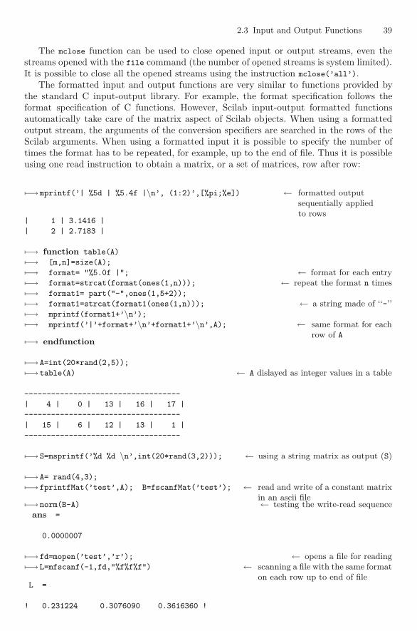
2.3 Input and Output Functions 39
The mclose function can be used to close opened input or output streams, even thestreams opened with the file command (the number of opened streams is system limited).It is possible to close all the opened streams using the instruction mclose(’all’).
The formatted input and output functions are very similar to functions provided bythe standard C input-output library. For example, the format specification follows theformat specification of C functions. However, Scilab input-output formatted functionsautomatically take care of the matrix aspect of Scilab objects. When using a formattedoutput stream, the arguments of the conversion specifiers are searched in the rows of theScilab arguments. When using a formatted input it is possible to specify the number oftimes the format has to be repeated, for example, up to the end of file. Thus it is possibleusing one read instruction to obtain a matrix, or a set of matrices, row after row:
�−→ mprintf(’| %5d | %5.4f |\n’, (1:2)’,[%pi;%e]) ← formatted outputsequentially appliedto rows
| 1 | 3.1416 |
| 2 | 2.7183 |
�−→ function table(A)
�−→ [m,n]=size(A);
�−→ format= "%5.0f |"; ← format for each entry�−→ format=strcat(format(ones(1,n))); ← repeat the format n times�−→ format1= part("-",ones(1,5+2));
�−→ format1=strcat(format1(ones(1,n))); ← a string made of ‘‘-’’�−→ mprintf(format1+’\n’);�−→ mprintf(’|’+format+’\n’+format1+’\n’,A); ← same format for each
row of A�−→ endfunction
�−→ A=int(20*rand(2,5));
�−→ table(A) ← A dislayed as integer values in a table
-----------------------------------
| 4 | 0 | 13 | 16 | 17 |
-----------------------------------
| 15 | 6 | 12 | 13 | 1 |
-----------------------------------
�−→ S=msprintf(’%d %d \n’,int(20*rand(3,2))); ← using a string matrix as output (S)
�−→ A= rand(4,3);
�−→ fprintfMat(’test’,A); B=fscanfMat(’test’); ← read and write of a constant matrixin an ascii file�−→ norm(B-A) ← testing the write-read sequence
ans =
0.0000007
�−→ fd=mopen(’test’,’r’); ← opens a file for reading�−→ L=mfscanf(-1,fd,"%f%f%f") ← scanning a file with the same format
on each row up to end of fileL =
! 0.231224 0.3076090 0.3616360 !

40 2 Introduction to Scilab
! 0.216463 0.932962 0.292227 !
! 0.883389 0.214601 0.5664250 !
! 0.6525130 0.3126420 0.482647 !
�−→ norm(L-A) ← note that numerical precision depends on selected format directivesans =
0.0000007
�−→ mclose(fd); ← close the opened file
The next example describes a formatted input where strings and scalars are mixed ina file that contains information on some Scicos files. The file mfscanf.dat is the following
An example of reading a file with a separator of type ’[ ]*,[ ]*’
-------------------------------------------------------------------------
CLKIN_f.sci , 98 , 16
CLKINV_f.sci , 91 , 16
CLOCK_f.sci , 116 , 16
CONST_f.sci , 50 , 8
CURV_f.sci , 80 , 12
We now illustrate how to use the function mfscanf to read out separately the numericaland the string information in this file.
�−→ fd=mopen(’mfscanf.dat’,’r’); ← opens a file in read mode�−→ mgetl(fd,2); ← bypassing the first two lines�−→ [n,a,b,c]=mfscanf(-1,fd,’%[^,],%*[, ]%d%*[, ]%d\ n’); ← formatted read
�−→ n ← number of read argumentsans =
3.
�−→ stripblanks(a)’ ← removing spaces and tranposing string matrixans =
!CLKIN_f.sci CLKINV_f.sci CLOCK_f.sci CONST_f.sci CURV_f.sci !
�−→ [b,c] ← numerical valuesans =
! 98. 16. !
! 91. 16. !
! 116. 16. !
! 50. 8. !
! 80. 12. !
�−→ mclose(fd); ← close the opened file stream
2.3.3 Input Output in Binary Mode
Scilab has its own binary internal format for saving Scilab objects and Scilab graphicsin a machine-independent way. It is possible to save variables in a binary file from the
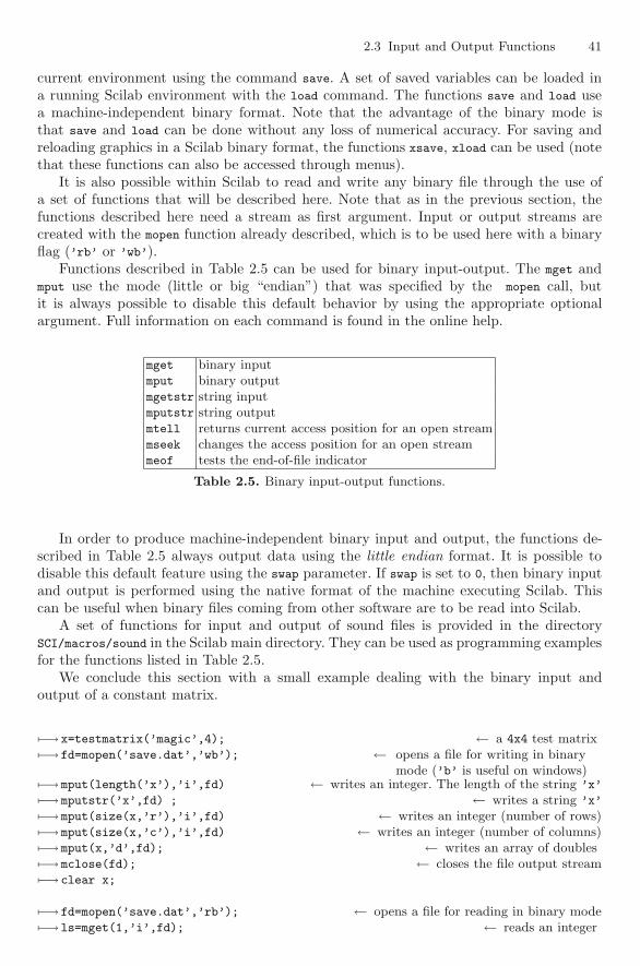
2.3 Input and Output Functions 41
current environment using the command save. A set of saved variables can be loaded ina running Scilab environment with the load command. The functions save and load usea machine-independent binary format. Note that the advantage of the binary mode isthat save and load can be done without any loss of numerical accuracy. For saving andreloading graphics in a Scilab binary format, the functions xsave, xload can be used (notethat these functions can also be accessed through menus).
It is also possible within Scilab to read and write any binary file through the use ofa set of functions that will be described here. Note that as in the previous section, thefunctions described here need a stream as first argument. Input or output streams arecreated with the mopen function already described, which is to be used here with a binaryflag (’rb’ or ’wb’).
Functions described in Table 2.5 can be used for binary input-output. The mget andmput use the mode (little or big “endian”) that was specified by the mopen call, butit is always possible to disable this default behavior by using the appropriate optionalargument. Full information on each command is found in the online help.
mget binary inputmput binary outputmgetstr string inputmputstr string outputmtell returns current access position for an open streammseek changes the access position for an open streammeof tests the end-of-file indicator
Table 2.5. Binary input-output functions.
In order to produce machine-independent binary input and output, the functions de-scribed in Table 2.5 always output data using the little endian format. It is possible todisable this default feature using the swap parameter. If swap is set to 0, then binary inputand output is performed using the native format of the machine executing Scilab. Thiscan be useful when binary files coming from other software are to be read into Scilab.
A set of functions for input and output of sound files is provided in the directorySCI/macros/sound in the Scilab main directory. They can be used as programming examplesfor the functions listed in Table 2.5.
We conclude this section with a small example dealing with the binary input andoutput of a constant matrix.
�−→ x=testmatrix(’magic’,4); ← a 4x4 test matrix�−→ fd=mopen(’save.dat’,’wb’); ← opens a file for writing in binary
mode (’b’ is useful on windows)�−→ mput(length(’x’),’i’,fd) ← writes an integer. The length of the string ’x’
�−→ mputstr(’x’,fd) ; ← writes a string ’x’
�−→ mput(size(x,’r’),’i’,fd) ← writes an integer (number of rows)�−→ mput(size(x,’c’),’i’,fd) ← writes an integer (number of columns)�−→ mput(x,’d’,fd); ← writes an array of doubles�−→ mclose(fd); ← closes the file output stream�−→ clear x;
�−→ fd=mopen(’save.dat’,’rb’); ← opens a file for reading in binary mode�−→ ls=mget(1,’i’,fd); ← reads an integer
42 2 Introduction to Scilab
�−→ name=mgetstr(ls,fd); ← reads a string. The string length is given by ls
�−→ m=mget(1,’i’,fd);n=mget(1,’i’,fd); ← reads two integers m and n
�−→ data=mget(m*n,’d’,fd); ← reads m*n doubles in a vector�−→ code= msprintf(’%s=matrix(data,%d,%d);’,name,m,n);
�−→ execstr(code); ← reshape the matrix and give it the correct name (i.e, x)�−→ mclose(fd) ; ← close the file�−→ and(x == testmatrix(’magic’,4)) ← test
ans =
T
2.3.4 Accessing the Host System
As already noted, formatted and binary inputs and outputs use streams to access or createfiles. Streams are created and opened through the command mopen and closed using themclose (or through the file command for Fortran-compatible streams). File streams areopened given a file pathname, which is coded as a Scilab string and can be absolute orrelative. The preferred syntax for file names is the Posix-style syntax (which works onWindows operating systems as well), i.e., with a slash as directory separator. If neces-sary, the pathconvert function can be used for pathname translation. Note that a relativepathname is always considered relative to the Scilab current directory. The name of thiscurrent directory is returned by the function getcwd or pwd and can be changed using thechdir or cd function. Given a pathname, it is possible to access the information about afile using the fileinfo function. For example, fileinfo(’foo’)<>[] will evaluate to %t iffile ’foo’ exists. Finally, the list of files in a given directory can be obtained as a vectorstring using the commands ls, dir, and listfiles.
It is possible obtain information through global Scilab variables about the runningScilab program, in particular on the operating system it was built for and the embeddedprograms that were used at compilation. For example, the boolean variable %tk can beused to check wether the current Scilab version is built with interaction with Tcl/Tk (Seealso %gtk for Gtk support and %pvm for parallel virtual machine support). MSDOS is a booleanvariable used to check wether the underlying operating system is Windows or a Unix-likesystem.
Running a shell script from Scilab is done using unix and related commands unix_g,unix_s (equivalently host), unix_w, and unix_x. These functions differ from each other inthe way they return the result of the command: in the current Scilab window (unix andunix_w), in a graphics widget (unix_x), in a Scilab variable (unix_g), or without returnedresult (unix_s). Note that contrary to what their names suggest, these commands work onUnix, Mac, and Windows operating systems.
It is sometimes useful to use the MSDOS variable before using the unix command sincethe syntax of shell commands differs between Unix and Windows. This is illustrated inthe following script:
�−→ %tk ← checks wether we have Tcl/Tk supportans =
T
�−→ MSDOS ← is it a Windows version of Scilab ?

2.3 Input and Output Functions 43
ans =
F
�−→ if ~MSDOS then�−→ os=unix_g(’uname’);
�−→ else�−→ os=’windows";
�−→ end�−→ os ← Operating system name ?
ans =
Linux
�−→ if MSDOS then�−→ l=unix_g(’dir sc*.sci’); ← list directory contents�−→ else�−→ l=unix_g(’ls sc*.sci’); ← list directory contents�−→ end�−→ l
l =
!scalarbase.sci !
! !
!scalarops.sci !
! !
!scalar.sci !
2.3.5 Graphical User Interface
So far, we have described input-output interaction with Scilab through keyboard inter-action in the Scilab graphics command window or through predefined menus. It is alsopossible to interact with Scilab through dialog windows and to create specific dialog win-dows. We will discuss how to do this here.
Scilab menus (in the command window and in the graphics windows) can be customizedusing Scilab commands. addmenu, delmenu, setmenu, or unsetmenu can be respectively usedto add, delete, activate, or deactivate Scilab menus. One can associate a menu han-dler to a specified menu through a Scilab function. For example addmenu(’foo’) (resp.addmenu(’foo’,4)) will place a menu button foo in the Scilab command window (resp.graphics window 4), which when activated will call Scilab function foo (resp. foo_4).
A set of predefined popup dialog windows are also available in Scilab. Some examplesare given in Figure 2.1. The simplest one is x_message, which is used to open a popupmessage window. Others are x_choose, which is used to perform a selection in a predefinedlist; x_dialog, which opens a dialog to get a response from the user as a Scilab string;x_choices, which is used to select a set of items each one being chosen through a togglelist; x_mdialog, which is used for a set of x_dialog-like interactions or for acquiring amatrix; and xgetfile, which is a dialog used to get a file path.
�−→ rep=x_choose([’S.L.Campbell’,’J.P.Chancelier’,’R.Nikoukhah’],’Authors’);
�−→ x_message([’Well, it’’s time ’;’to get something to eat !’]);
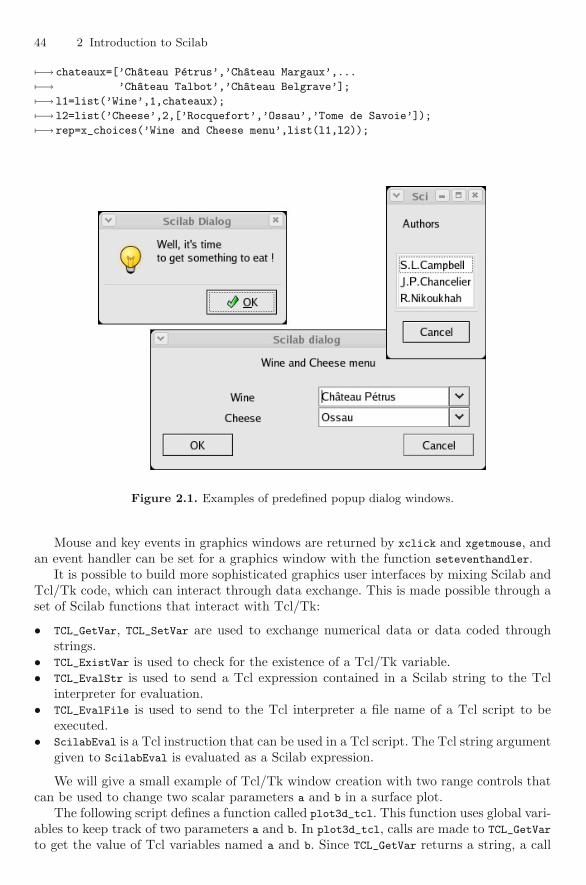
44 2 Introduction to Scilab
�−→ chateaux=[’Chateau Petrus’,’Chateau Margaux’,...
�−→ ’Chateau Talbot’,’Chateau Belgrave’];
�−→ l1=list(’Wine’,1,chateaux);
�−→ l2=list(’Cheese’,2,[’Rocquefort’,’Ossau’,’Tome de Savoie’]);
�−→ rep=x_choices(’Wine and Cheese menu’,list(l1,l2));
Figure 2.1. Examples of predefined popup dialog windows.
Mouse and key events in graphics windows are returned by xclick and xgetmouse, andan event handler can be set for a graphics window with the function seteventhandler.
It is possible to build more sophisticated graphics user interfaces by mixing Scilab andTcl/Tk code, which can interact through data exchange. This is made possible through aset of Scilab functions that interact with Tcl/Tk:
• TCL_GetVar, TCL_SetVar are used to exchange numerical data or data coded throughstrings.
• TCL_ExistVar is used to check for the existence of a Tcl/Tk variable.• TCL_EvalStr is used to send a Tcl expression contained in a Scilab string to the Tcl
interpreter for evaluation.• TCL_EvalFile is used to send to the Tcl interpreter a file name of a Tcl script to be
executed.• ScilabEval is a Tcl instruction that can be used in a Tcl script. The Tcl string argument
given to ScilabEval is evaluated as a Scilab expression.
We will give a small example of Tcl/Tk window creation with two range controls thatcan be used to change two scalar parameters a and b in a surface plot.
The following script defines a function called plot3d_tcl. This function uses global vari-ables to keep track of two parameters a and b. In plot3d_tcl, calls are made to TCL_GetVar
to get the value of Tcl variables named a and b. Since TCL_GetVar returns a string, a call

2.3 Input and Output Functions 45
to evstr is made to evaluate the string. If a or b in the Scilab environment differs fromthe Tcl/Tk values, then the Scilab values are updated and a surface is drawn. Graphicswill be discussed in more detail in Section 2.4. Here we just note that plot3d will draw asurface and that the drawing of the surface depends on the two Scilab parameters a andb. Thus, if a or b is changed at the Tcl/Tk level, then a call to plot3d_tcl will draw a newsurface. Note that a flicker effect will be seen in the graphics window when redrawing isperformed. We will see in Section 2.4 how to avoid this.
function []=plot3d_tcl()
global(’a’,’b’);
a_new=evstr(TCL_GetVar("a"));
b_new=evstr(TCL_GetVar("b"));
if a<>a_new | b<>b_new thena=a_new ; b = b_new ;
t=linspace(0,2,200);
xbasc();t=linspace(-b*%pi,b*%pi,20);plot3d(t,t,a*sin(t)’*cos(t));
endendfunction
This function can be checked now with the following, which plots the surface:
�−→ TCL_SetVar(’a’,’3’); ← setting a to 3 in Tcl/Tk�−→ TCL_SetVar(’b’,’2’); ← setting b to 3 in Tcl/Tk�−→ plot3d_tcl();
Now we want a dialog window with two range controls in order to change the valuesof a and b interactively. This can be done as described in the next Tcl/Tk script.
# tcl/tk scripttoplevel .topwm resizable .top 0 0;set a 5;set b 2;#—————————-wm title .top {tk test};global ok wait but;proc runScilab {bidon} {ScilabEval plot3d tcl()};#—– top labelframe .top.widtoplabel .top.widlabel −text {Surface parameters}pack .top.widlabel −in .top.widtop −side top −pady 5#—- a range control for aframe .top.wid frame2label .top.widlabel a −text {a}scale .top.widscale a −variable a −width 8 −state normal −from 1 −to 10 \
−resolution .01 −orient horizontal −width 8 −command {runScilab}pack .top.widlabel a −in .top.wid frame2 −side left −anchor w −padx 5 \
−expand truepack .top.widscale a −in .top.wid frame2 −side left −anchor e −padx 5#—– a range control for b

46 2 Introduction to Scilab
frame .top.wid frame3label .top.widlabel b −text {b}scale .top.widscale b −variable b −width 8 −state normal −from 1 −to 3 \
−resolution .01 −orient horizontal −width 8 −command {runScilab}pack .top.widlabel b −in .top.wid frame3 −side left −anchor w −padx 5 \
−expand truepack .top.widscale b −in .top.wid frame3 −side left −anchor e −padx 5#——————-pack .top.widtop −in .toppack .top.wid frame2 −in .toppack .top.wid frame3 −in .top#——————-raise .top
This is a pure Tcl/Tk script, wich is mostly independent of Scilab except for thefact that we call the ScilabEval function when a range control is changed. As alreadymentioned, ScilabEval is a Tcl function that sends its argument as a Scilab expression tothe Scilab interpreter. Here, as expected, the ScilabEval function will send to the Scilabinterpreter the string ’plot3d_tcl()’. Thus a range control modification will lead to a callto the plot3d_tcl function.
In order to launch the Tcl/Tk script we use TCL_EvalFile at the Scilab level. A pictureof the Tcl/Tk dialog is provided in Figure 2.2
�−→ TCL_EvalFile("range.tcl"); ← running the Tcl/Tk script from Scilab
For a restricted set of Tcl/Tk dialogs predefined in Scilab and called uicontrols, theprocess we have just described can be simplified in the sense that the Tcl/Tk script can bereplaced by a Scilab script using the figure, uicontrol, and uimenu functions. The rangecontrols used in the previous example are part of this restricted set of Tcl/Tk dialogs. Wewill now give the same example of a surface drawing but now managed through uicontrols.The function plot3d_uicontrol is the function that is activated when a range control (alsocalled slider in uicontrol manual pages) is changed (this is called a callback), and thefunction myuidialog is used to build the Tcl/Tk window with the two sliders and the twotext areas that display the sliders’ values. The two functions share data through globalScilab variables. A picture of the Tcl/Tk dialog composed with uicontrols is provided inFigure 2.3
function plot3d_uicontrol()
global(’a_slider’,’a_text’,’b_slider’,’b_text’,’a’,’b’,’activate’,’n_fact’);
if activate == %t thena=get(a_slider,’Value’)/n_fact;
b=get(b_slider,’Value’)/n_fact;
set(a_text,’String’,’a=’+string(a))
set(b_text,’String’,’b=’+string(b))
t=linspace(0,2,200);
xbasc();t=linspace(-b*%pi,b*%pi,20);plot3d(t,t,a*sin(t)’*cos(t));
endendfunction

2.3 Input and Output Functions 47
Figure 2.2. Example of a Tcl/Tk dialog.
function myuidialog()
global(’a_slider’,’a_text’,’b_slider’,’b_text’,’a’,’b’,’activate’,’n_fact’);
n_fact=100; ← scaling because sliders work with integersactivate=%f ; ← delay callback executionf = figure("Position",[50 50 200 60],"Unit", "pixel");
a_text = uicontrol(f,"Position",[140 10 55 15],"Style","text",...
"String" , "a=5")
a_slider = uicontrol(f, "Position" , [10 10 120 15],..
"Style" , "slider",...
"Min" , 1*n_fact,...
"Max" , 10*n_fact,...
"Value" , 5*n_fact,...
"SliderStep", [1 1],...
"callback" , "plot3d_uicontrol()")
b_text = uicontrol(f, "Position",[140 35 55 15],"Style","text",...
"String" , "b=2")
b_slider = uicontrol(f, "Position" , [10 35 120 15],...
"Style" , "slider",...
"Min" , 1*n_fact,...
"Max" , 3*n_fact,...
"Value" , 2*n_fact,...
"SliderStep", [1 1],...
"callback" , "plot3d_uicontrol()")
activate=%t; ← now we accept callback callsendfunction
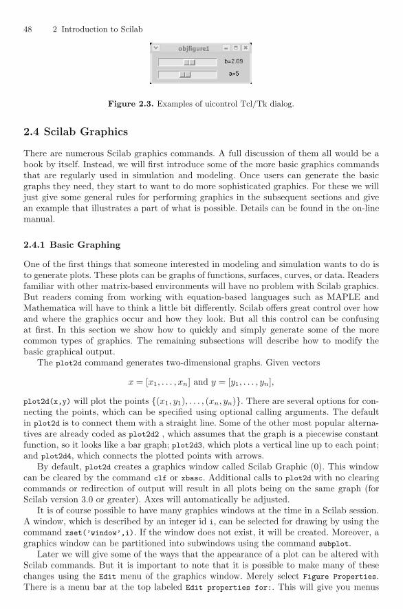
48 2 Introduction to Scilab
Figure 2.3. Examples of uicontrol Tcl/Tk dialog.
2.4 Scilab Graphics
There are numerous Scilab graphics commands. A full discussion of them all would be abook by itself. Instead, we will first introduce some of the more basic graphics commandsthat are regularly used in simulation and modeling. Once users can generate the basicgraphs they need, they start to want to do more sophisticated graphics. For these we willjust give some general rules for performing graphics in the subsequent sections and givean example that illustrates a part of what is possible. Details can be found in the on-linemanual.
2.4.1 Basic Graphing
One of the first things that someone interested in modeling and simulation wants to do isto generate plots. These plots can be graphs of functions, surfaces, curves, or data. Readersfamiliar with other matrix-based environments will have no problem with Scilab graphics.But readers coming from working with equation-based languages such as MAPLE andMathematica will have to think a little bit differently. Scilab offers great control over howand where the graphics occur and how they look. But all this control can be confusingat first. In this section we show how to quickly and simply generate some of the morecommon types of graphics. The remaining subsections will describe how to modify thebasic graphical output.
The plot2d command generates two-dimensional graphs. Given vectors
x = [x1, . . . , xn] and y = [y1, . . . , yn],
plot2d(x,y) will plot the points {(x1, y1), . . . , (xn, yn)}. There are several options for con-necting the points, which can be specified using optional calling arguments. The defaultin plot2d is to connect them with a straight line. Some of the other most popular alterna-tives are already coded as plot2d2 , which assumes that the graph is a piecewise constantfunction, so it looks like a bar graph; plot2d3, which plots a vertical line up to each point;and plot2d4, which connects the plotted points with arrows.
By default, plot2d creates a graphics window called Scilab Graphic (0). This windowcan be cleared by the command clf or xbasc. Additional calls to plot2d with no clearingcommands or redirection of output will result in all plots being on the same graph (forScilab version 3.0 or greater). Axes will automatically be adjusted.
It is of course possible to have many graphics windows at the time in a Scilab session.A window, which is described by an integer id i, can be selected for drawing by using thecommand xset(’window’,i). If the window does not exist, it will be created. Moreover, agraphics window can be partitioned into subwindows using the command subplot.
Later we will give some of the ways that the appearance of a plot can be altered withScilab commands. But it is important to note that it is possible to make many of thesechanges using the Edit menu of the graphics window. Merely select Figure Properties.There is a menu bar at the top labeled Edit properties for:. This will give you menus
2.4 Scilab Graphics 49
for all the more important properties. The most commonly used ones are probably Axes
and Polyline.There are a number of ways to control the flow of Scilab output. Here we note that the
Scilab graphics window has a file button. If clicked, it provides an easy way to export thegraph into a number of formats including postscript. Note also that the graphics windowhas a zoom button, which allows you to select part of the graph and zoom in on it.
The fact that the graphics routines start with matrices sometimes creates problems.For example
�−→ tt=0:0.1:3;plot2d(tt,sin(tt));
will generate the graph of sin(t) on the interval [0, 3]. However,
�−→ function y=myf(t);y=sin(t)*sin(t);endfunction;
�−→ tt=0:0.1:3;plot2d(tt,f(tt))
will produce an error message and not the graph of sin2(t). The problem is that the functionmyf has to be able to take the vector tt and evaluate it entry by entry. The following codewill generate the graph of sin2(t):
�−→ function y=myf(t);y=sin(t).*sin(t);endfunction
�−→ tt=0:0.1:3;plot2d(tt,f(tt))
Note that the function is defined using elementwise multiplication .* instead of *.A number of graphs created using the basic versions of plot2d and some of its features
can be found in Chapter 3Plots of a surface z = f(x, y) can be done in two ways. The scilab command plot3d
works much like plot2d in that it has the syntax plot3d(x,y,z), where x, y, z are vectors.However, there is also the function fplot3d, which has the basic syntax fplot3d(x,y,f),where f is an external of the type y=f(x,y). Here x and y determine the grid on which f willbe evaluated. The default for plot3d and fplot3d is for the graph to appear in a graphicswindow. Again the window can be exported into a postscript figure file by using one of thefile options. Another useful feature is the 3D Rot. button of the graphics window. If thisbutton is clicked, then one can click and hold on the figure, rotate using the mouse, andthen click to release the figure. While the viewing point of the figure can also be adjustedby using optional calling arguments, it is usually easiest to find the best viewing angle byusing the 3D Rot. option. Surface plots can be altered using the Edit menu of the graphicswindow just as 2D plots are.
2.4.2 Graphic Tour
We start with a number of scripts to make a tour of Scilab graphics functionalities. Twographics styles coexist in Scilab today. But most high-level graphical functions are usedin a similar fashion in both styles, so the examples provided in this first part work withboth, as did the examples of the previous section. We shall later focus on the differencesof the two styles and, in particular, present the object-oriented aspects of the new style.
Parametric Curve Plot in R3
The parametric plot of (sin(t), t cos(t)/R, t/100) on [−20π, 20π] using a uniform grid of2000 points with R = 20π is created by
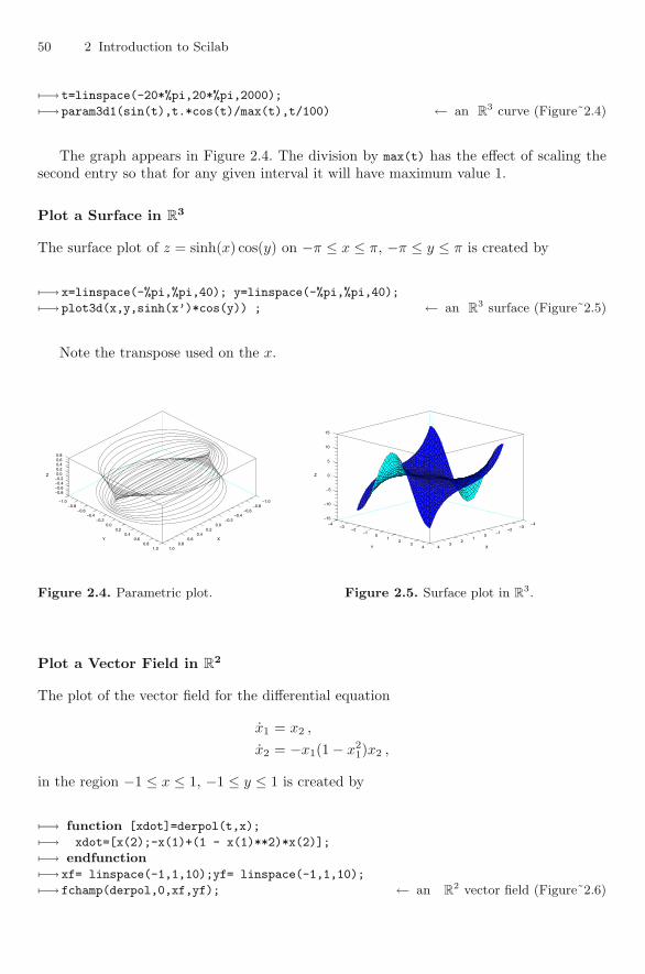
50 2 Introduction to Scilab
�−→ t=linspace(-20*%pi,20*%pi,2000);
�−→ param3d1(sin(t),t.*cos(t)/max(t),t/100) ← an R3 curve (Figure˜2.4)
The graph appears in Figure 2.4. The division by max(t) has the effect of scaling thesecond entry so that for any given interval it will have maximum value 1.
Plot a Surface in R3
The surface plot of z = sinh(x) cos(y) on −π ≤ x ≤ π, −π ≤ y ≤ π is created by
�−→ x=linspace(-%pi,%pi,40); y=linspace(-%pi,%pi,40);
�−→ plot3d(x,y,sinh(x’)*cos(y)) ; ← an R3 surface (Figure˜2.5)
Note the transpose used on the x.
−0.8−0.6−0.4−0.20.00.20.40.60.8
Z
−1.0−0.8
−0.6−0.4
−0.20.0
0.20.4
0.60.8
1.0
X
−1.0−0.8
−0.6−0.4
−0.20.0
0.20.4
0.60.8
1.0
Y
−15
−10
−5
0
5
10
15
Z
−4−3
−2−1
01
23
4 X
−4−3
−2−1
01
23
4Y
Figure 2.4. Parametric plot. Figure 2.5. Surface plot in R3.
Plot a Vector Field in R2
The plot of the vector field for the differential equation
x1 = x2 ,
x2 = −x1(1 − x21)x2 ,
in the region −1 ≤ x ≤ 1, −1 ≤ y ≤ 1 is created by
�−→ function [xdot]=derpol(t,x);
�−→ xdot=[x(2);-x(1)+(1 - x(1)**2)*x(2)];
�−→ endfunction�−→ xf= linspace(-1,1,10);yf= linspace(-1,1,10);
�−→ fchamp(derpol,0,xf,yf); ← an R2 vector field (Figure˜2.6)

2.4 Scilab Graphics 51
Plot a Histogram
Generating a random vector with a normal distribution, plotting this vector as a histogram,and then plotting the normal distribution on the same graph is given by the following:
�−→ v=rand(1,2000,’n’);
�−→ histplot([-6:0.4:6],v,[1],’015’,’ ’,[-4,0,4,0.5],[2,2,2,1]); ← a histogram�−→ function [y]=f2(x); y=exp(-x.*x/2)/sqrt(2*%pi); endfunction;�−→ x=-6:0.1:6;x=x’;plot2d(x,f2(x),1); ← superimposing an R
2 curve (Figure˜2.7)
−1.0 −0.8 −0.6 −0.4 −0.2 0.0 0.2 0.4 0.6 0.8 1.0−1.0
−0.8
−0.6
−0.4
−0.2
0.0
0.2
0.4
0.6
0.8
1.0
−4 40
Figure 2.6. A vector field. Figure 2.7. A histogram.
Polar Plot in R2
The plot in polar coordinates of ρ = sin(2θ) cos(2θ) for 0 ≤ θ ≤ 2π is created by thefollowing commands:
�−→ theta=0:.01:2*%pi;rho=sin(2*theta).*cos(2*theta);
�−→ polarplot(theta,rho); ← an R2 curve in polar coordinates (Figure˜2.8)
Plot a Surface Given by Facets in R3
If a surface in R3 is parameterized by two variables, then by assigning a grid to these two
variables we can create a surface composed of facets. This is illustrated below.
�−→ function [x,y,z]=f3(alpha,theta)
�−→ x=cos(alpha).*cos(theta);
�−→ y=cos(alpha).*sin(theta);
�−→ z=sinh(alpha);
�−→ endfunction�−→ alphagrid=linspace(-%pi/2,%pi/2,40);thetagrid=linspace(0,2*%pi,20);
�−→ [x1,y1,z1]=eval3dp(f3, alphagrid, thetagrid); ← building a set of facets�−→ plot3d1(x1,y1,z1); ← an R
3 surface composed by a set of facets (Figure˜2.9)
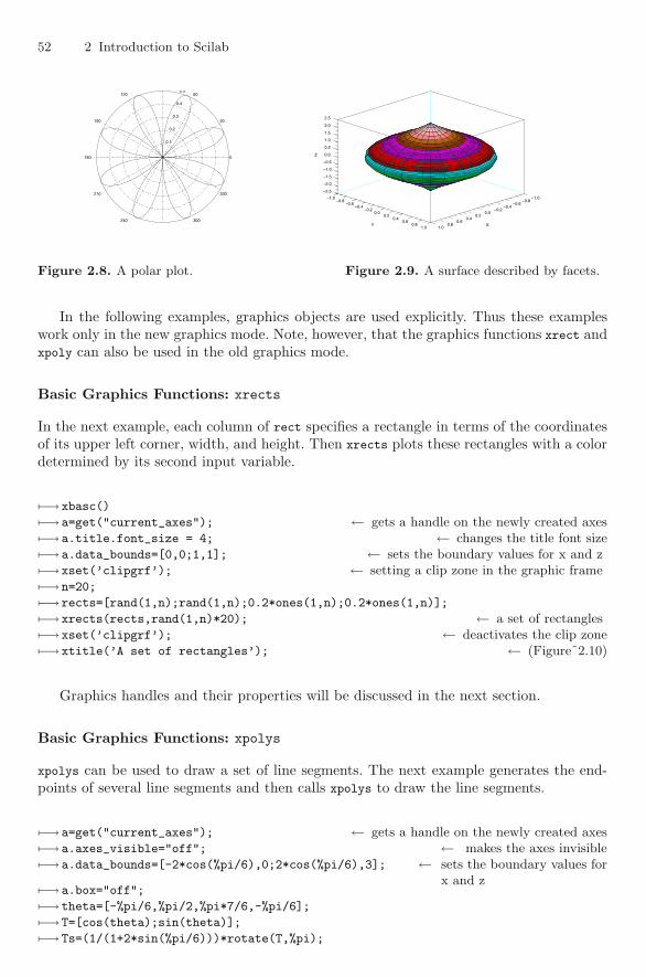
52 2 Introduction to Scilab
0.1
0.2
0.3
0.4
0.5
0
30
60120
150
180
210
240 300
330−2.5
−2.0
−1.5
−1.0
−0.5
0.0
0.5
1.0
1.5
2.0
2.5
Z
−1.0−0.8
−0.6−0.4
−0.20.0
0.20.4
0.60.8
1.0X
−1.0−0.8
−0.6−0.4
−0.20.0
0.20.4
0.60.8
1.0Y
Figure 2.8. A polar plot. Figure 2.9. A surface described by facets.
In the following examples, graphics objects are used explicitly. Thus these exampleswork only in the new graphics mode. Note, however, that the graphics functions xrect andxpoly can also be used in the old graphics mode.
Basic Graphics Functions: xrects
In the next example, each column of rect specifies a rectangle in terms of the coordinatesof its upper left corner, width, and height. Then xrects plots these rectangles with a colordetermined by its second input variable.
�−→ xbasc()
�−→ a=get("current_axes"); ← gets a handle on the newly created axes�−→ a.title.font_size = 4; ← changes the title font size�−→ a.data_bounds=[0,0;1,1]; ← sets the boundary values for x and z�−→ xset(’clipgrf’); ← setting a clip zone in the graphic frame�−→ n=20;
�−→ rects=[rand(1,n);rand(1,n);0.2*ones(1,n);0.2*ones(1,n)];
�−→ xrects(rects,rand(1,n)*20); ← a set of rectangles�−→ xset(’clipgrf’); ← deactivates the clip zone�−→ xtitle(’A set of rectangles’); ← (Figure˜2.10)
Graphics handles and their properties will be discussed in the next section.
Basic Graphics Functions: xpolys
xpolys can be used to draw a set of line segments. The next example generates the end-points of several line segments and then calls xpolys to draw the line segments.
�−→ a=get("current_axes"); ← gets a handle on the newly created axes�−→ a.axes_visible="off"; ← makes the axes invisible�−→ a.data_bounds=[-2*cos(%pi/6),0;2*cos(%pi/6),3]; ← sets the boundary values for
x and z�−→ a.box="off";
�−→ theta=[-%pi/6,%pi/2,%pi*7/6,-%pi/6];
�−→ T=[cos(theta);sin(theta)];
�−→ Ts=(1/(1+2*sin(%pi/6)))*rotate(T,%pi);
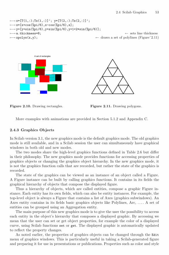
2.4 Scilab Graphics 53
�−→ x=[T(1,:);Ts(1,:)]’; y=[T(2,:);Ts(2,:)]’;
�−→ x=[x+cos(%pi/6),x-cos(%pi/6),x];
�−→ y=[y+sin(%pi/6),y+sin(%pi/6),y+1+2*sin(%pi/6)];
�−→ a.thickness=8; ← sets line thickness�−→ xpolys(x,y); ← draws a set of polylines (Figure˜2.11)
A set of rectangles
Figure 2.10. Drawing rectangles. Figure 2.11. Drawing polygons.
More examples with animations are provided in Section 5.1.2 and Appendix C.
2.4.3 Graphics Objects
In Scilab version 3.1, the new graphics mode is the default graphics mode. The old graphicsmode is still available, and in a Scilab session the user can simultaneously have graphicalwindows in both old and new modes.
The two modes share the high-level graphics functions defined in Table 2.6 but differin their philosophy. The new graphics mode provides functions for accessing properties ofgraphics objects or changing the graphics object hierarchy. In the new graphics mode, itis not the graphics function calls that are recorded, but rather the state of the graphics isrecorded.
The state of the graphics can be viewed as an instance of an object called a Figure.A Figure instance can be built by calling graphics functions. It contains in its fields thegraphical hierarchy of objects that compose the displayed figure.
Thus a hierarchy of objects, which are called entities, compose a graphic Figure in-stance. Each entity has its own fields, which can also be entity instances. For example, thetop-level object is always a Figure that contains a list of Axes (graphics subwindows). AnAxes entity contains in its fields basic graphics objects like Polylines, Arc, . . . . A set ofentities can be grouped using an Aggregation entity.
The main purpose of this new graphics mode is to give the user the possibility to accesseach entity in the object’s hierarchy that composes a displayed graphic. By accessing wemean that the user can set or get object properties, for example the color of a displayedcurve, using Scilab functions set or get. The displayed graphic is automatically updatedto reflect the property changes.
As noted earlier, the properties of graphics objects can be changed through the Edit
menu of graphics windows. This is particularly useful in taking a Scilab-generated figureand preparing it for use in presentations or publications. Properties such as color and style

54 2 Introduction to Scilab
of lines and graphs are found under the properties of Polyline. A slide will adjust the color.The axis style and labeling are under the properties of Axes.
Thus, from the user point of view, a Figure can be viewed as an instance of a dynamictree object. The nodes of the tree are called entities. The user can change the graph byadding or deleting nodes and changing the node properties. The Scilab name of a nodepointer is a handle.
The two graphics modes can coexist in a Scilab session, but a default mode is set bythe Scilab startup: set("old_style","off"|"on") can be used to set the default mode, andset("figure_style","new"|"old") can be used to open a graphical window in the specifiedmode.
We will now give some examples showing some of the graphics entities in action.In this first example a graphics window is created, a default scale is set by calling
plot2d, and a rectangle is drawn. In order to change the rectangle’s properties, we firstneed to get a handle on it. Since the rectangle is the last drawn object, it is the currententity of the current graphics window, and in that case r=get("hdl") is the easiest way toaccess the rectangle. It is then possible to change the displayed rectangle’s properties.
�−→ a=get("current_axes"); ← get a handle on the newly created axes�−→ a.data_bounds=[-1,-1;1,1]; ← set the boundary values for x and z�−→ xrect(0,0,0.5,0.5) ← draw a rectangle�−→ r=get("hdl"); ← get the current node, i.e, the last created objects�−→ r ← r is a handle to a Rectangle entity
ans =
Handle of type "Rectangle" with properties:
===========================================
parent: Axes
children: []
mark_mode = "off"
mark_style = 0
mark_size_unit = "tabulated"
mark_size = 0
mark_foreground = -1
mark_background = -2
line_mode = "on"
line_style = 0
thickness = 1
fill_mode = "off"
foreground = -1
data = [0,0,0.5,0.5]
visible = "on"
clip_state = "off"
clip_box = []
�−→ r.fill_mode="on"; ← changing the displayed rectangle’s properties�−→ r.foreground=5;
�−→ r_line_style=6;
In order to illustrate entities navigation, we can accomplish the same thing as theprevious example in a more complex way by navigating, from node to node, in the graphof the objects associated with the figure.
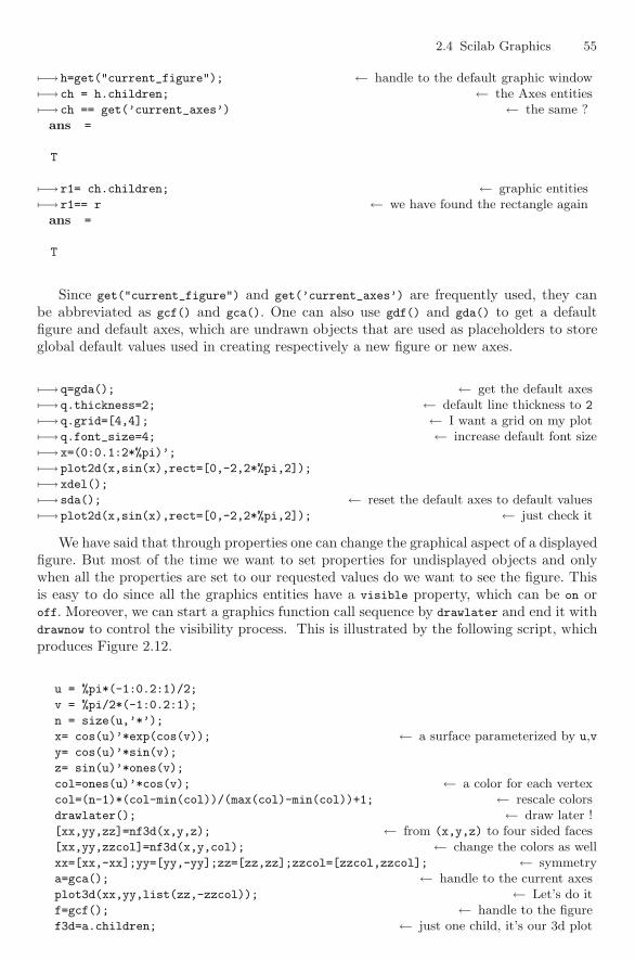
2.4 Scilab Graphics 55
�−→ h=get("current_figure"); ← handle to the default graphic window�−→ ch = h.children; ← the Axes entities�−→ ch == get(’current_axes’) ← the same ?
ans =
T
�−→ r1= ch.children; ← graphic entities�−→ r1== r ← we have found the rectangle again
ans =
T
Since get("current_figure") and get(’current_axes’) are frequently used, they canbe abbreviated as gcf() and gca(). One can also use gdf() and gda() to get a defaultfigure and default axes, which are undrawn objects that are used as placeholders to storeglobal default values used in creating respectively a new figure or new axes.
�−→ q=gda(); ← get the default axes�−→ q.thickness=2; ← default line thickness to 2
�−→ q.grid=[4,4]; ← I want a grid on my plot�−→ q.font_size=4; ← increase default font size�−→ x=(0:0.1:2*%pi)’;
�−→ plot2d(x,sin(x),rect=[0,-2,2*%pi,2]);
�−→ xdel();
�−→ sda(); ← reset the default axes to default values�−→ plot2d(x,sin(x),rect=[0,-2,2*%pi,2]); ← just check it
We have said that through properties one can change the graphical aspect of a displayedfigure. But most of the time we want to set properties for undisplayed objects and onlywhen all the properties are set to our requested values do we want to see the figure. Thisis easy to do since all the graphics entities have a visible property, which can be on oroff. Moreover, we can start a graphics function call sequence by drawlater and end it withdrawnow to control the visibility process. This is illustrated by the following script, whichproduces Figure 2.12.
u = %pi*(-1:0.2:1)/2;
v = %pi/2*(-1:0.2:1);
n = size(u,’*’);
x= cos(u)’*exp(cos(v)); ← a surface parameterized by u,vy= cos(u)’*sin(v);
z= sin(u)’*ones(v);
col=ones(u)’*cos(v); ← a color for each vertexcol=(n-1)*(col-min(col))/(max(col)-min(col))+1; ← rescale colorsdrawlater(); ← draw later ![xx,yy,zz]=nf3d(x,y,z); ← from (x,y,z) to four sided faces[xx,yy,zzcol]=nf3d(x,y,col); ← change the colors as wellxx=[xx,-xx];yy=[yy,-yy];zz=[zz,zz];zzcol=[zzcol,zzcol]; ← symmetrya=gca(); ← handle to the current axesplot3d(xx,yy,list(zz,-zzcol)); ← Let’s do itf=gcf(); ← handle to the figuref3d=a.children; ← just one child, it’s our 3d plot

56 2 Introduction to Scilab
f3d.hiddencolor=n; ← set the hidden face’s colorsa.rotation_angles = [55,110]; ← set the view anglesf.color_map= graycolormap(n); ← set the colormapdrawnow(); ← show the result in a graphics window
−1.0−0.8−0.6−0.4−0.20.00.20.40.60.81.0
Z
−1.0−0.8
−0.6−0.4
−0.20.0
0.20.4
0.60.8
1.0Y
−3
−2
−1
0
1
2
3
X
Figure 2.12. plot3d with the new graphic.
For those who prefer a graphical interface, keep in mind that an Edit button is availablein the graphics window menu, which when launched opens up Tcl/Tk menus that can beused to navigate and change graphical object properties.
Tables 2.6, 2.7, and 2.8 summarize the Scilab graphics functions, graphics primitives,and graphics window primitives respectively.
2.4.4 Scilab Graphics and LATEX
This section is for those interested in inserting Scilab graphics into LATEX documents [23](the typesetting system used to produce this book).
Inserting a Scilab graphic in a LATEX document is an easy task since Scilab can exportgraphics as Postscript files and there are commands in LATEX to include Postscript files.Exporting a scilab graphic to Postscript can be, as already noted, achieved through theFile menu of the graphics window, but it is also possible to use the Scilab command xs2eps
(or xs2ps and the program BEpsf) to generate a Postscript file.However, sometimes one wants to have a figure that is a mixture of Scilab graphics
images and LATEX mathematical expressions. This can require translating the Postscriptstrings inserted in a Postscript document to LATEX commands in order, for example, toget mathematical expressions inserted in a graphic. There exists a LATEX package namedpsfrag that facilitates this task. Using psfrag you can substitute strings present in thePostscript file by LATEX expressions. The idea is to position strings in Scilab graphics
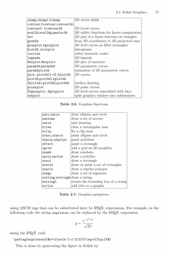
2.4 Scilab Graphics 57
champ,champ1,fchamp 2D vector fieldscontour,fcontour,contour2d,contourf, fcontour2d 2D Level curveseval3d,eval3dp,genfac3d 3D utility functions for facets computationfec 2D plot of a linear function on trianglesgeom3d from 3D coordinates to 2D projected onesgrayplot,fgrayplot 2D level curves as filled rectangleshist3d, histplot histogramsisoview select isometric scaleslegends 2D legendsMatplot,Matplot1 2D plot of matricesparam3d,param3d1 3D parametric curvesparamfplot2d animation of 2D parametric curvesplot, plot2d[1-4],fplot2d 2D curvesplot3d,plot3d1,fplot3d,fplot3d1,plot3d2,plot3d3 surface drawingpolarplot 2D polar curvesSfgrayplot, Sgrayplot 2D level curves (smoothed with fec)subplot split graphics window into subwindows
Table 2.6. Graphics functions.
xarc,xarcs draw ellipses and circlexarrows draw a set of arrowsxaxis axis drawingxclea clear a rectangular zonexclip fix a clip zonexfarc,xfarcs paint ellipses and circlexfpoly,xfpolys paint polylinesxfrect paint a rectanglexgrid add a grid on 2D graphicsxnumb draw numbersxpoly,xpolys draw a polylinexrect draw a rectanglexrects draw or paint a set of rectanglesxrpoly draw a regular polygonxsegs draw a set of segmentsxstring,xstringb draw a stringxstringl return the bounding box of a stringxtitle add title to a graphic
Table 2.7. Graphics primitives.
using ASCII tags that can be substituted later by LATEX expressions. For example, in thefollowing code the string exprlatex can be replaced by the LATEX expression
y =e−x2/2
√2π
using the LATEX code
\psfrag{exprlatex}{$y=\frac{e^{-x^2/2}}{\sqrt{2\pi}}$}
This is done by generating the figure in Scilab by
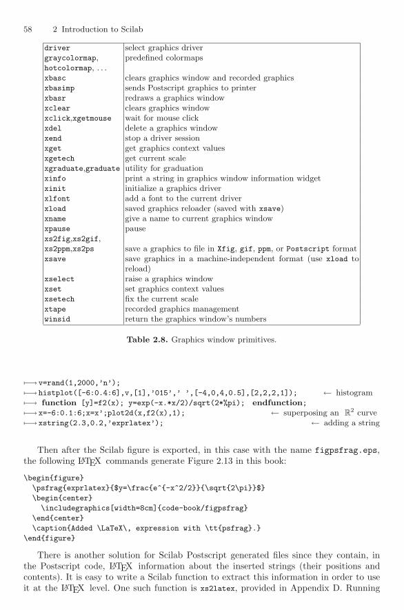
58 2 Introduction to Scilab
driver select graphics drivergraycolormap,hotcolormap, . . .
predefined colormaps
xbasc clears graphics window and recorded graphicsxbasimp sends Postscript graphics to printerxbasr redraws a graphics windowxclear clears graphics windowxclick,xgetmouse wait for mouse clickxdel delete a graphics windowxend stop a driver sessionxget get graphics context valuesxgetech get current scalexgraduate,graduate utility for graduationxinfo print a string in graphics window information widgetxinit initialize a graphics driverxlfont add a font to the current driverxload saved graphics reloader (saved with xsave)xname give a name to current graphics windowxpause pausexs2fig,xs2gif,xs2ppm,xs2ps save a graphics to file in Xfig, gif, ppm, or Postscript formatxsave save graphics in a machine-independent format (use xload to
reload)xselect raise a graphics windowxset set graphics context valuesxsetech fix the current scalextape recorded graphics managementwinsid return the graphics window’s numbers
Table 2.8. Graphics window primitives.
�−→ v=rand(1,2000,’n’);
�−→ histplot([-6:0.4:6],v,[1],’015’,’ ’,[-4,0,4,0.5],[2,2,2,1]); ← histogram�−→ function [y]=f2(x); y=exp(-x.*x/2)/sqrt(2*%pi); endfunction;�−→ x=-6:0.1:6;x=x’;plot2d(x,f2(x),1); ← superposing an R
2 curve�−→ xstring(2.3,0.2,’exprlatex’); ← adding a string
Then after the Scilab figure is exported, in this case with the name figpsfrag.eps,the following LATEX commands generate Figure 2.13 in this book:
\begin{figure}
\psfrag{exprlatex}{$y=\frac{e^{-x^2/2}}{\sqrt{2\pi}}$}
\begin{center}
\includegraphics[width=8cm]{code-book/figpsfrag}
\end{center}
\caption{Added \LaTeX\, expression with \tt{psfrag}.}
\end{figure}
There is another solution for Scilab Postscript generated files since they contain, inthe Postscript code, LATEX information about the inserted strings (their positions andcontents). It is easy to write a Scilab function to extract this information in order to useit at the LATEX level. One such function is xs2latex, provided in Appendix D. Running
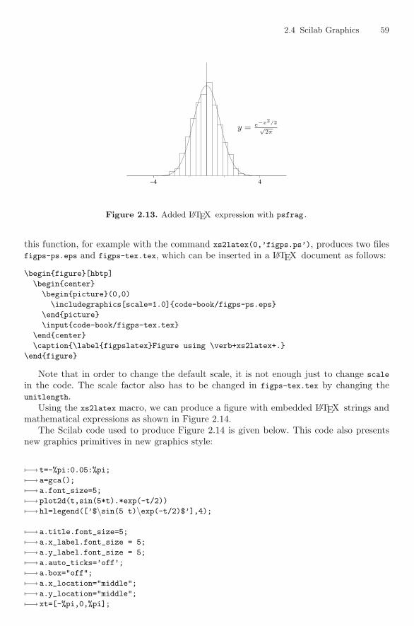
2.4 Scilab Graphics 59
−4 4
y = e−x2/2√2π
Figure 2.13. Added LATEX expression with psfrag.
this function, for example with the command xs2latex(0,’figps.ps’), produces two filesfigps-ps.eps and figps-tex.tex, which can be inserted in a LATEX document as follows:
\begin{figure}[hbtp]
\begin{center}
\begin{picture}(0,0)
\includegraphics[scale=1.0]{code-book/figps-ps.eps}
\end{picture}
\input{code-book/figps-tex.tex}
\end{center}
\caption{\label{figpslatex}Figure using \verb+xs2latex+.}
\end{figure}
Note that in order to change the default scale, it is not enough just to change scale
in the code. The scale factor also has to be changed in figps-tex.tex by changing theunitlength.
Using the xs2latex macro, we can produce a figure with embedded LATEX strings andmathematical expressions as shown in Figure 2.14.
The Scilab code used to produce Figure 2.14 is given below. This code also presentsnew graphics primitives in new graphics style:
�−→ t=-%pi:0.05:%pi;
�−→ a=gca();
�−→ a.font_size=5;
�−→ plot2d(t,sin(5*t).*exp(-t/2))
�−→ hl=legend([’$\sin(5 t)\exp(-t/2)$’],4);
�−→ a.title.font_size=5;
�−→ a.x_label.font_size = 5;
�−→ a.y_label.font_size = 5;
�−→ a.auto_ticks=’off’;
�−→ a.box="off";
�−→ a.x_location="middle";
�−→ a.y_location="middle";
�−→ xt=[-%pi,0,%pi];
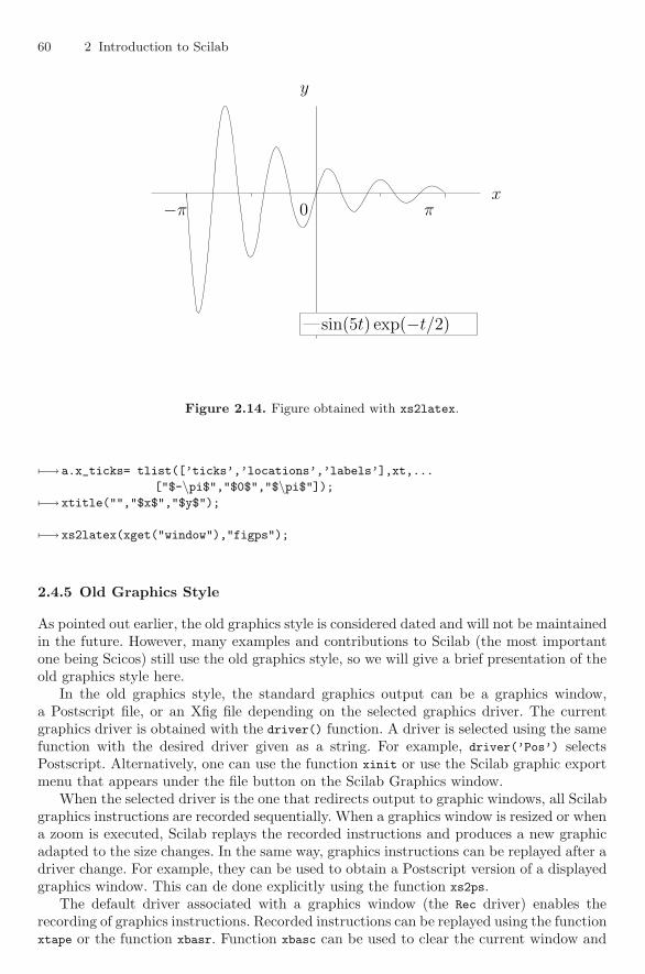
60 2 Introduction to Scilab
x
y
−π 0 π
sin(5t) exp(−t/2)
Figure 2.14. Figure obtained with xs2latex.
�−→ a.x_ticks= tlist([’ticks’,’locations’,’labels’],xt,...
["$-\pi$","$0$","$\pi$"]);�−→ xtitle("","$x$","$y$");
�−→ xs2latex(xget("window"),"figps");
2.4.5 Old Graphics Style
As pointed out earlier, the old graphics style is considered dated and will not be maintainedin the future. However, many examples and contributions to Scilab (the most importantone being Scicos) still use the old graphics style, so we will give a brief presentation of theold graphics style here.
In the old graphics style, the standard graphics output can be a graphics window,a Postscript file, or an Xfig file depending on the selected graphics driver. The currentgraphics driver is obtained with the driver() function. A driver is selected using the samefunction with the desired driver given as a string. For example, driver(’Pos’) selectsPostscript. Alternatively, one can use the function xinit or use the Scilab graphic exportmenu that appears under the file button on the Scilab Graphics window.
When the selected driver is the one that redirects output to graphic windows, all Scilabgraphics instructions are recorded sequentially. When a graphics window is resized or whena zoom is executed, Scilab replays the recorded instructions and produces a new graphicadapted to the size changes. In the same way, graphics instructions can be replayed after adriver change. For example, they can be used to obtain a Postscript version of a displayedgraphics window. This can de done explicitly using the function xs2ps.
The default driver associated with a graphics window (the Rec driver) enables therecording of graphics instructions. Recorded instructions can be replayed using the functionxtape or the function xbasr. Function xbasc can be used to clear the current window and
2.4 Scilab Graphics 61
to clear the associated recorded graphics instructions. Destroying a graphics window byclicking or by calling xdel also clears the associated recorded graphics.
It can sometimes be useful to use a graphics window without graphic recording, forexample during animations. This is easily done by switching to the driver X (or W).
The default graphics behavior is that graphics display appears as soon as a graphicsfunction is called. It is possible to attach a pixmap to a graphics window in order to redirectgraphics outputs to that pixmap. The graphics window is redrawn using the pixmap statusby a user specific command.
The pixmap mode of a graphics window is a window graphics parameter, and eachgraphics window has a large set of parameters. They define the graphics context of agraphics window. Many graphics windows can coexist, but only the graphics context ofthe current graphics window can be changed. The ID of the current graphics window (whichis an integer) can be obtained using xget(’window’), and changing the graphics windowis done with xset(’window’,n). The graphic context parameters of the current graphicswindow are obtained with the function xget and changed using the function xset.
The pixmap mode can be very useful, in particular for animation, so let us considerit more carefully. This mode is selected by calling xset(’pixmap’,1). As explained earlier,when this mode is selected, graphics are directed to a pixmap. The content of the pixmapis copied to the graphics window when the xset(’wshow’) instruction is executed. Thepixmap used for graphics is cleared by calling wset(’wwpc’). This mode can be used forgraphics animations since it avoids the flicker caused by having to clear a graphics windowbefore redrawing it. The following script generates a movie of a rectangle that moves andchanges its color pattern.
set old_style on
xsetech(frect=[0,0,10,10])
xrect(0,10,10,10)
n=100;
xset(’pixmap’,1)
driver(’X11’);
for k=-n:n,
a=ones(n,n);
a= 3*tril(a,k)+ 2*a;
a= a + a’;
k1= 3*(k+100)/200;
Matplot1(a,[k1,2,k1+7,9])
xset(’wshow’)
xset(’wwpc’)
endxset(’pixmap’,0)
The final point concerns scale computations. Graphics functions that aim at drawingsimple objects, for example rectangles xrects, or polylines xpoly, use the current graphicsscale. It is good scilab programming to set a graphics scale before calling such functionseven if no error messages are provided by Scilab if the scales are not set. A current scale isset each time a high-level graphics function is called, such as plot2d, or when an explicitcall to the function xsetech is used.
The default behavior of high-level functions is to adapt the current graphics scale so asto remain compatible with previous graphics function calls. But optional parameters canbe used to change this default behavior. This is illustrated by the next example, whichgenerates the graphs in Figure 2.15 and Figure 2.16.
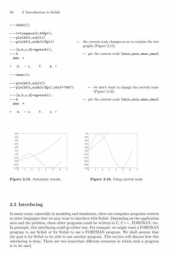
62 2 Introduction to Scilab
�−→ xbasc();
�−→ t=linspace(0,2*%pi);
�−→ plot2d(t,sin(t))
�−→ plot2d(t,sinh(t/%pi)) ← the current scale changes so as to contain the twographs (Figure˜2.15)
�−→ [a,b,c,d]=xgetech();
�−→ b ← get the current scale [xmin,ymin,xmax,ymax]
ans =
! 0. - 1. 7. 4. !
�−→ xbasc();
�−→ plot2d(t,sin(t))
�−→ plot2d(t,sinh(t/%pi),strf="000") ← we don’t want to change the current scale(Figure˜2.16)
�−→ [a,b,c,d]=xgetech();
�−→ b ← get the current scale [xmin,ymin,xmax,ymax]
ans =
! 0. - 1. 7. 1. !
0 1 2 3 4 5 6 7−1.0
−0.5
0.0
0.5
1.0
1.5
2.0
2.5
3.0
3.5
4.0
0 1 2 3 4 5 6 7−1.0
−0.8
−0.6
−0.4
−0.2
0.0
0.2
0.4
0.6
0.8
1.0
Figure 2.15. Automatic rescale. Figure 2.16. Using current scale.
2.5 Interfacing
In many areas, especially in modeling and simulation, there are computer programs writtenin other languages that we may want to interface with Scilab. Depending on the applicationarea and the problem, these other programs could be written in C, C++, FORTRAN, etc.In principle, this interfacing could go either way. For example, we might want a FORTRANprogram to use Scilab or for Scilab to use a FORTRAN program. We shall assume thatthe goal is for Scilab to be able to use another program. This section will discuss how thisinterfacing is done. There are two somewhat different scenarios in which such a programis to be used.
2.5 Interfacing 63
The first scenario is that the outside program is being called from within a Scilabfunction. For example, the outside program might return the value of the right-hand sideof the differential equation that we wish to integrate with Scilab’s ordinary differentialsolver ode. In that case, the interface is somewhat simpler and is described in Subsection2.5.1.
In the second scenario we wish to have the given program become a Scilab functionthat we want to be able to call and use just like any other built-in Scilab function. Thisis discussed in Sections 2.5.2 and 2.5.3 it will often require some knowledge of the Cprogramming language and the language used by the given external program.
2.5.1 Linking Code
Writing an interface is not always necessary in order to access external code. Suppose,for example, that you want to create a new Scicos block whose behavior is described byC-code. You do not need to access your block from the Scilab interpreter since the callwill be performed directly by Scicos’s internal simulator. In this case what you need isjust to link your external code and update the Scilab internal table of dynamically linkedfunctions. Then Scicos will be able to access the new code.
In fact, most of the Scilab functions that accept an external as argument can use thedynamic linking facility to access externally coded functions. We note ode, dassl, optim,and fsolve. Of course, when using this facility the calling sequence of the external functionis constrained by the function it will be passed to. Each external-aware function has itsown imposed calling sequence. There’s also a special Scilab primitive called call, whichcan be used to call from the Scilab interpreter a dynamically linked routine that has in itsarguments just integer, double, or character pointers. It can be used for testing externalcode. Just as in the previous section, we still have to create a shared library and load itin Scilab.
Linking external code can be done in two different ways. The function addinter is usedto add new primitives to Scilab and requires the writing of interfaces. The function link
just adds a new entry in the internal Scilab table of external functions. As pointed outearlier, such entries can be used by some Scilab primitives. Here we will use the link
command through the ilib_for_link encapsulation. We encapsulate the call to dlaswp inanother function to simplify the number of requested arguments:
#include <string.h>#include "stack-c.h"
extern int C2F(dlaswp)(int *n,double *A,int *lda,int *k1,int *k2,int *ipiv,int *step);
int dlaswp1(double *A,int *m,int *n,int *mipiv,int *ipiv){
const int un =1;C2F(dlaswp)(n,A,m,&un,mipiv,ipiv,&un);
}
We can compile the code using a small Scilab script called builder.sce (a more precisedescription of builders is given in Section2.5.3) :
�−→ names=[’dlaswp1’]; // entry points
64 2 Introduction to Scilab
�−→�−→ files = ’dlaswp1.o’; // object files
�−→ flag = ’c’ ;
�−→ ilib_for_link(names,files,[],"c");
generate a loader file
generate a Makefile: Makelib
running the makefile
compilation of dlaswp1
building shared library (be patient)
In the previous code flag=’c’ is just there to specify that the function dlaswp is aC-coded function. This is used to guess the proper naming convention of entry points. Weload the code in a running Scilab with the generated loader.sce file:
�−→ // generated by builder.sce: Please do not edit this file
�−→ // ------------------------------------------------------
�−→ dlaswp1_path=get_absolute_file_path(’loader.sce’);
�−→ link(dlaswp1_path+’libdlaswp1.so’,[’dlaswp1’],’c’);
shared archive loaded
Link done
Now we can call the newly linked function not directly, but, for example, throughthe call function. The call function plays the role of the interface for a small subset ofargument types. For example, we can call dlaswp as follows:
shared archive loaded
Link done
�−→ perm=[1,3,4,3];mp=size(perm,’*’);
�−→ A=eye(4,4);[m,n]=size(A);
�−→ y=call("dlaswp1",A,1,"d",m,2,"i",n,3,"i",mp,4,"i",perm,5,"i","out",1)
y =
! 1. 0. 0. 0. !
! 0. 0. 1. 0. !
! 0. 1. 0. 0. !
! 0. 0. 0. 1. !
The first call argument is the name of the function to be called. It is the name thatwas given to the link command as the entry point name. Other arguments from A to "out"
give information on the arguments that are to be passed to dlaswp1. Then the argumentsthat follow the keyword "out" give information about returned values.
Each transmitted argument is described by three entries. For example, A,1,"d" meansthat the first argument of dlaswp1 is an array of double (precision) that points to the dataof matrix A. The 1 that follows the "out" keyword means that the first returned value isalso the first argument.
To provide a more explicit example, suppose that you want to find a zero of thenonlinear equation cos(x)x2 − 1 = 0. You can build a Scilab function:

2.5 Interfacing 65
�−→ function y=f(x)
�−→ y=cos(x)*x^2-1
�−→ endfunction
and using fsolve and the function f as its argument try to find a zero numerically:
�−→ y0=10; y=fsolve(y0,f)
y =
11.003833
�−→ f(y)
ans =
3.819D-14
However, we shall use this problem to illustrate linking. Suppose that the function f
is C-coded (for example for efficiency) and it respects the calling convention of the Scilabfsolve primitive. One such implementation of f would be the following C-code:
#include <math.h>void f(int *n,double *x,double *fval,int *iflag){
*fval = cos(*x)*(*x)*(*x) − 1;}
As before, we build and load a shared library using ilib_for_link. Then we pass theproblem to solve to function fsolve by just giving a string that gives the name of the entrypoint to use, which in this problem is "f". The result is:
�−→ ilib_for_link(’f’,’f.o’,[],’c’);
generate a loader file
generate a Makefile: Makelib
running the makefile
compilation of f
building shared library (be patient)
shared archive loaded
Link done
�−→ y0=10; y=fsolve(y0,"f")
y =
11.003833
Many other Scilab functions can use C- and Fortran-coded functions directly, includingode, optim, etc.
66 2 Introduction to Scilab
2.5.2 Writing an Interface
The main purpose of this section is to show how to integrate C- compatible functions intoScilab. Suppose that we want to add new primitives to Scilab that will call external C-like functions. By C-like functions, we mean functions that can be coded in any languagethat remains compatible with C code in terms of linking and calling stack conventions.Examples include Fortran code and C++ (“extern C”) functions.
We start with two examples that are Fortran-coded functions from the LAPACK li-brary. [4] The first function is dgetrf, which performs an LU factorization of a givenmatrix. Given a m×n matrix A coded as an array of double-precision scalars of size m×n
and an integer array of size Max(m,n), denoted by ipiv, the dgetrf routine performs anin-place LU factorization of a matrix. In fact, the LU factorization can be done with rowinterchanges. The integer array ipiv is here just to retain a coding of the row permutation.A Fortran subroutine can be called from C code with the convention that all argumentsare transmitted through pointers. Note also that the naming conventions differ slightlyfrom C to Fortran and are compiler-dependent. We enclose the Fortran name in a C2F(.)
macro call, which will take care of naming conventions. Thus, the calling sequence fordgetrf from C-code is as follows:
extern int C2F(dgetrf)(int *m,int *n,double *A,int *lda,int *ipiv,int *info);
The second function we want to use is dlaswp. This routine simply applies a permutationdescribed by an ipiv integer array to a given matrix:
extern int C2F(dlaswp)(int *n,double *A,int *lda,int *k1,int *k2,int *ipiv,int *step);
In order to access these two functions we add two Scilab primitives also called dgetrf
and dlaswp with the following calling syntax:
[LU,perm]=dgetrf(A);
[C]=dlaswp(B,perm);
We still need to write glue code for converting Scilab arguments to C form, calling theexternal functions, and back-converting C objects to Scilab returned values. Most of thetime the glue code is written in C and is called an interface, so that an interface is just aC-function. We need an interface for each function to be included into Scilab.
The two interfaces for dgetrf and dlaswp are as follows:
#include <string.h>#include "stack-c.h"
extern int C2F(dgetrf)(int *m,int *n,double *A,int *lda,int *ipiv,int *info);
int int dgetrf(char *fname){
int l1, m1, n1, mipiv,nipiv=1,lipiv,info;CheckRhs(1,1);CheckLhs(1,2);GetRhsVar(1, "d", &m1, &n1, &l1);mipiv= Max(m1,n1);CreateVar(2, "i", &mipiv,&nipiv, &lipiv);C2F(dgetrf)(&m1,&n1,stk(l1),&m1,istk(lipiv),&info);if ( info < 0 )
2.5 Interfacing 67
{Scierror(999,"%s: argument %d of dgetrf has an illegal value\r\n",
fname,−info);return 0;
}else if ( info > 0 ){
sciprint("%s: U(%d,%d) is exactly zero\r\n",info+1,info+1);}
LhsVar(1) = 1;LhsVar(2) = 2;return 2;
}
#include <string.h>#include "stack-c.h"
extern int C2F(dlaswp)(int *n,double *A,int *lda,int *k1,int *k2,int *ipiv,int *step);
int int dlaswp(char *fname){
int l1, m1, n1, mipiv,nipiv,lipiv,info,un=1;CheckRhs(2,2);CheckLhs(1,2);GetRhsVar(1, "d", &m1, &n1, &l1);GetRhsVar(2, "i", &mipiv,&nipiv, &lipiv);mipiv= mipiv*nipiv;C2F(dlaswp)(&n1,stk(l1),&m1,&un,&mipiv,istk(lipiv),&un);LhsVar(1) = 1;return 1;
}
Note that in the two previous interfaces we have used functions, macros, or data fromthe interface library (CheckRhs, CheckLhs, GetRhsVar, CreateVar, and LhsVar). The headerfile stack-c.h is there to provide macro definitions and prototypes for the interface libraryfunctions.
At first sight, these two functions might seem complex, but most of the time we donot have to write the full interface from scratch. Picking pieces of code from the examplesprovided is the easiest way to write new functions. We won’t describe in full detail all thefunctions that are present in the interface library. Rather we will try to give the rules thatare to be followed for writing an interface.
How does the interface work? When at the Scilab level the user enters the command[LU,perm]=dgetrf(rand(5,5)), the arguments of the dgetrf function are first evaluated andtheir resulting values are stored in a stack (the function calling stack) in the order theyappear in the calling sequence. Here we just have one argument; rand(5,5) is evaluated andthe resulting matrix is stored on the calling stack at position 1. The Scilab calling sequenceis also analyzed by the interpreter in order to evaluate how many returned arguments areexpected. Here two returned arguments are expected.
The glue code for dgetrf, here called int_dgetrf, is then called by the interpreted code.The first job to be performed by the interface is to check that the number of given argu-ments is correct and that the number of expected returned arguments is also correct. This
68 2 Introduction to Scilab
is performed by CheckLhs and CheckRhs . For example, if the number of given argumentsis outside of the given bounds, then CheckRhs will print an error message and we returnfrom the interface to the Scilab interpreter with a Scilab error raised.
In the interface each variable present on the stack is characterized by an integer thatis its position on the stack. Calling arguments are, when entering the interface, stored onthe stack from position 1 to n if n is the number of given arguments.
The next job to be performed is to check that each given argument has the expectedtype and proper dimensions. If the type is correct, then we need to give a pointer to theassociated argument data. This pointer will be given to the C-function we are interfacing.The next command,
GetRhsVar(1, "d", &m1, &n1, &l1);
checks that the first given argument is a scalar matrix ("d") and, in case of success, returnsin m1 and n1 the matrix dimensions and in l1 an identifier that can be used to get a pointerto the double array data (stk(l1)).
Before calling the function dgetrf, we need to allocate space in the Scilab calling stackfor the integer array ipiv, which is to be of dimensions 1\timesMax(m1,n1). The C-code
mipiv= Max(m1,n1);
CreateVar(2, "i", &mipiv,&nipiv, &lipiv);
will create a scalar matrix with the proper size. The "i" is here to say that the arrayis to be considered as an integer array. Data access is done through an integer pointeristk(lipiv). Since the first available position is position 2, we use this position for ournewly created variable.
The calling syntax of CreateVar is the same as the calling syntax of GetRhsVar, but notethat in creating a variable, the dimension parameters are used as input data.
We are now ready to call the function dgetrf. After the call, the Scierror function canbe used to raise a Scilab error and the sciprint function can be used to display warningmessages or other relevant information.
After the call, we want to return the result of the LU factorization, which is storedin the double array stk(l1), and the coded permutation, which is stored in istk(lipiv).Notice that in dgetrf the double array stk(l1) is used as both input and output variable.However, there is no risk in modifying a Scilab input variable since when we are in theinterface GetRhsVar, we do not have direct access to a given argument but only to a copyof that argument. It is thus safe to modify the m1xn1 values of the double array stk(l1)
and to use this variable as a Scilab return value.We have checked at the beginning of the interface the number of requested returned
values. At the end we just have to indicate at which location on the stack the returnedarguments are to be found. The syntax LhsVar(i)=j is used to say that the ith value tobe returned is at position j on the stack.
The second variable to be returned is the integer array. Note that by default Scilabmatrices are stored as a double array and that we have used the data of the second variableas an integer array. Since we have declared that the second variable was an integer array("i"), Scilab will perform an automatic conversion of the array when returning from theinterface.
All interfaces are based on the same pattern, and a number of examples are availablein the subdirectories of SCI/examples. For example, the files included in the directorySCI/examples/interface-tour-so give a tour of almost all of the functions that can beused for interfacing. Note that it is possible, for example, to interface a function that itselfuses a function as a parameter and at the Scilab level we often want to pass a Scilab
2.5 Interfacing 69
function as an argument. It is also explained how to call the Scilab interpreter within aninterface to compute an intermediate value.
In the MATLAB world, interfaces are known under the name of mexfiles. As explainedin SCI/examples/mex-examples, mexfiles can be emulated in Scilab and can be used asinterfaces for Scilab functions.
2.5.3 Dynamic Loading
Writing glue code is just the first step. In order to use the desired code, we need tocompile the written code as a shared library. Usually this is .so files in Unix and .dll
files in Windows. Then we need to load it in Scilab, and tell Scilab the correspondencebetween the interface names and the names of primitives to be added. Since this processis system-dependent, we have developed Scilab script to hide system-dependent code fromthe Scilab user. We have two interface functions that are coded in the two files intdgetrf.cand intdlaswp.c. Note that there are no limitations or constraints on the number of filesand their names.
Using a text editor, we have to write a small Scilab script named builder.sce. This isa canonic name and most Scilab users know that running builder.sce is used to set up acontribution or an interface:
�−→ // This is the builder.sce that must be run from this directory
�−→ ilib_name = ’liblapack’; ← interface library name�−→ files = [’lapack.o’]; ← objects files�−→ libs = []; ← other libraries needed for linking�−→ table =[’dgetrf’, ’int_dgetrf’; ← association table (scilab˙name, interface-name)�−→ ’dlaswp’, ’int_dlaswp’];
�−→ // do not modify below
�−→ // ----------------------------------------------
�−→ ilib_build(ilib_name,table,files,libs)
Of course, one can use as a model the builder.sce file contained in the directorySCI/examples/interface-tutorial-so/builder.sce. It can be easily adapted to create anew interface.
builder.sce provides the following information:
• ilib_name is a string that stands for the library name (a set of interfaces) that we arebuilding.
• files is a string matrix that gives the object files that are needed to build the li-brary. Note that the object files are suffixed with .o even under Windows. A uniquebuilder.sce file is to be built and it should run as well under Unix and Windows.
• libs is a string matrix that gives a list of libraries (shared libraries) that are neededby the object files. Note that in our example, we are interfacing functions from theLAPACK library, which is an already loaded Scilab executable. Thus we do not needto provide object files or libraries for providing the code of the dgetrf and dlaswp
functions.• table is a string matrix, where the association between a Scilab name and an interface
name is provided. For example, its first line ’dgetrf’, ’int_dgetrf’; indicates thatthe Scilab function dgetrf is implemented via the interface int_dgetrf.
Running the builder.sce script from Scilab will create a shared library and a set ofnew files.
70 2 Introduction to Scilab
�−→ // This is the builder.sce that must be run from this directory
�−→ ilib_name = ’liblapack’; ← interface library name�−→ files = [’lapack.o’]; ← objects files�−→ libs = []; ← other libraries needed for linking
�−→ table =[’dgetrf’, ’int_dgetrf’; ← association table (scilab˙name, interface-name)�−→ ’dlaswp’, ’int_dlaswp’];
�−→ // do not modify below
�−→ // ----------------------------------------------
�−→ ilib_build(ilib_name,table,files,libs)
generate a gateway file
generate a loader file
generate a Makefile: Makelib
running the makefile
compilation of lapack
building shared library (be patient)
Among the created files, the most important one is a new Scilab script calledloader.sce, which can be used when we need to load the shared library in a runningScilab. The loader.sce uses the Scilab function addinter to load the shared library andupdate the primitive table.
In practice, one executes the builder.sce once. Note that when running a builder.sce
script the current Scilab directory must be the directory containing the builder.sce script,and the library is loaded with the loader.sce script each time we start a new Scilab session.
�−→ // generated by builder.sce: Please do not edit this file
�−→ // ------------------------------------------------------
�−→ liblapack_path=get_file_path(’loader.sce’);
�−→ functions=[ ’dgetrf’;
�−→ ’dlaswp’;
�−→ ];
�−→ addinter(liblapack_path+’/liblapack.so’,’liblapack’,functions);
shared archive loaded
Among the other generated files we note:
• A file named after the library name liblapack.c, called a “gateway” file, is also gen-erated. It contains the main entry point of the library, which is used by the addinter
function.• A makefile named Makelib, which is system-dependent and, which can be used to
rebuild the shared library. This makefile can be very useful for debugging purposeswhen the shared library build process fails.
We can now test the added primitives:
�−→ exec (’loader.sce’);
shared archive loaded
�−→ A=rand(5,5);

2.5 Interfacing 71
�−→ B=A;
�−→ [LU,perm]=dgetrf(A); ← call dgetrf�−→ [E]=dlaswp(eye(A),perm); ← apply permutation to identity matrix�−→ L=tril(LU,-1)+eye(LU);U=triu(LU); ← separate L and U
�−→ if norm(L*U-E*A) > 10*%eps then pause; end ; ← check result
3
Modeling and Simulation in Scilab
One of the fundamental problems in many areas of science and engineering is the problemof modeling and simulation. Scilab provides a large array of tools for developing andsimulating models of several types. For several of these tools it is possible to use themwith abbreviated commands and default values of some parameters. However, to knowhow to choose the appropriate tools and how to get the kind of answers desired, it is oftennecessary to know something about how the algorithms are set up and what to do if thereare difficulties.
In this chapter we shall describe the types of models that are available in Scilab andsome of the tools available for their simulation. We shall also give some general commentsabout how to use the tools and how to choose between the tools.
3.1 Types of Models
3.1.1 Ordinary Differential Equations
One of the most popular types of model is that of ordinary differential equations (ODE)such as
y = f(t, y). (3.1)
Here y and f may be vector valued, y is a function of the real variable t, and y denotesthe derivative of y with respect to t. System (3.1) is a first-order equation since it involvesonly first-order derivatives.
Some models are initially formulated in terms of higher derivatives, but they can alwaysbe rewritten as first-order systems by the introduction of additional variables. The Scilabtools assume that the differential equation has first been rewritten to be of first order.The exception to this is boundary value problems, where the numerical methods allow forhigher-order differential equations.
Example 1. The system of second-oder differential equations
y1 = y1 − y2 + sin(t), (3.2a)y2 = 3y1 + y1 − 4y2, (3.2b)
can be rewritten as
74 3 Modeling and Simulation in Scilab
y1 = y3, (3.3a)y2 = y4, (3.3b)y3 = y3 − y2 + sin(t), (3.3c)y4 = 3y3 + y1 − 4y2. (3.3d)
The differential equation (3.1) generally has a family of solutions. To perform a sim-ulation, additional information must be provided to make the solution unique. An initialcondition is the value of y at a particular value of t. A boundary condition is when morethan one value of t is involved in the additional conditions. An example of a boundarycondition is y(0) − 2y(π) = 0. We will discuss boundary value problems later.
The basic existence and uniqueness result for differential equations in the form (3.1)says that if we specify y(t0), and f and fy = ∂f/∂y are continuous functions of t and ynear (t0, y(t0)), then there is a unique solution to (3.1) satisfying the initial condition. Thesolution will continue to exist as long as these assumptions hold. Another important factis that the more derivatives of f(t, y) that exist and are continuous, the more derivativesy has.
This may seem to be an esoteric fact, but it actually plays an important role in simula-tion. The reason is that most simulation tools try to deliver a requested accuracy and theerror estimates are based on assumptions about the number of derivatives of the solutions.Suppose now that we have a controlled differential equation
y = f(t, y, u(t)) (3.4)
with u(t) a given function. Then even if f has all the derivatives that one wants, y canhave only one more derivative than u. Thus if a control is only piecewise continuous,so that it has jumps, which often occurs in applications, the solution y will not have acontinuous first derivative at the jumps. This in turn can lead to serious problems withmany numerical tools unless the behavior of u is taken into account when one is requestingthe simulation.
3.1.2 Boundary Value Problems
Boundary value problems (BVP) are differential equations but with the information givenat two or more times rather than at just one time. Two-point boundary value problemstake the general form of
y = f(t, y), t0 ≤ t ≤ tf , (3.5a)0 = B(y(t0), y(tf )). (3.5b)
If y in (3.5a) is n-dimensional, then there usually need to be n equations in (3.5b) in orderto uniquely determine a solution. However, the theory is more complicated than that forinitial value problems, as illustrated by the next example.
Example 2. Suppose that we have the boundary value problem
y =(
0 1−1 0
)y +
(01
), (3.6a)
0 =(
y1(0)y2(tf )
). (3.6b)
The solution of this differential equation is
3.1 Types of Models 75
y1 = c1 cos(t) + c2 sin(t) + 1, (3.7a)y2 = −c1 sin(t) + c2 cos(t), (3.7b)
where c1, c2 are arbitrary constants. The first boundary condition (3.7a) gives c1 = −1.The second boundary condition (3.7b) then gives that
0 = sin(tf ) + c2 cos(tf ). (3.8)
But (3.8) has a solution for c2 only if cos(tf ) �= 0. Thus we see that the existence of asolution to this boundary value problem depends on the particular value of tf . Here tfcannot be π
2 + mπ, where m is an integer.
One of the nice features about ODEs is that the given initial conditions are at onepoint. This means that with the numerical methods given below the computation can belocal and move from one step to the next. This makes it easier to solve problems on longertime intervals or with higher state dimension. With BVP, since the information occurs atmore than one time, it is often necessary to use a more global algorithm that takes intoaccount the full t interval. This leads to much larger systems of equations that have to besolved.
3.1.3 Difference Equations
The second major class of models is that of difference equations. These problems occurwhen there a quantity whose values are of interest only at discrete-time values or thevalues change only at discrete times. Difference equations can occur either because theprocess is naturally discrete and only undergoes changes at isolated times or because itis continuous but our observations occur only at isolated times. Also, many numericalmethods for differential equations actually solve an approximating difference equation.
In difference equations there is an integer variable, which we denote by k. The solutionis a sequence y(k) and it has to solve a difference equation
y(k + 1) = f(k, y(k)), y(k0) = y0. (3.9)
Sometimes it is more natural to think of a sequence of times tk, k ≥ k0, and a differenceequation
z(tk+1) = g(tk, z(tk)), z(tk0) = z0. (3.10)
If the tk are evenly spaced, so that t+1− tk = h where h is a constant, then we can rewrite(3.10) in the form of (3.9) as follows:
v(k + 1) = g(w(k), v(k)), v(k0) = z0, (3.11a)w(k + 1) = w(k) + h, w(k0) = tk0 . (3.11b)
Note that v(k) of (3.11a) is the same as z(tk) from (3.10).For the remainder of this section we will assume that the difference equation is in
the form (3.9). The theory for solutions of difference equations is simpler than that fordifferential equations. Given a starting time k0 and a value of y0 that gives the initialcondition y(k0) = y0, the values of y(k) for k > k0 are computed recursively using (3.9)and will exist as long as (k, y(k)) is in the domain of f .
There is one important difference between the discrete and continuous theories thatis worth mentioning. The uniqueness theorem for differential equations tells us that iftwo solutions start at the same time but with different initial values and if the continuityassumptions on f, fy are holding, then the solutions can never intersect. This is not truefor difference equations.
76 3 Modeling and Simulation in Scilab
Example 3. The difference equation (3.12) is at the origin after two time steps no matterwhere it starts at k0:
y(k + 1) =(
1 −11 −1
)y(k). (3.12)
The difference equations (3.9) and (3.12) are of first order since there is maximaldifference of one in the values of k that are present. Just as systems of differential equationscan always be written as first-order differential equations, difference equations can alwaysbe written as first-order difference equations.
Example 4. The equation (3.13) is of third order since (k + 3) − k = 3:
y(k + 3) = 4y(k + 2) − y(k + 1)y(k). (3.13)
The difference equation (3.13) can be rewritten as a first-order difference equation byintroducing additional variables as shown in (3.14):
y1(k + 1) = y2(k), (3.14a)y2(k + 1) = y3(k), (3.14b)y3(k + 1) = 4y3(k) − y2(k)y1(k). (3.14c)
The Scilab tools for working with difference equations assume that they have beenwritten in first-order form.
3.1.4 Differential Algebraic Equations
Many physical systems are most naturally initially modeled by systems composed of bothdifferential and algebraic equations [11]. These systems take the general form of
F (t, y, y) = 0 (3.15)
and are often called DAEs.
Example 5. One example of a DAE is a model of a constrained mechanical system wherethe constraint is on the position variables. Such a system takes the general form
x = v, (3.16a)v = G(x, v, t) + Q(x, t)λ, (3.16b)0 = H(x, t). (3.16c)
System (3.16) is a DAE in y = (x, v, λ). Equation (3.16c) gives the constraints. AlsoQ(x, t) = Hx(x, t)T , and Q(x, t)λ gives the force generated by the constraint.
Given a DAE model, there are two options. One option is to try to rewrite the DAEinto an ODE or a simpler DAE. This is usually done by a mixture of differentiation andalgebraic manipulations. The other option is to try to simulate the DAE directly.
The theory for DAEs is much more complex than the theory for ODEs. One problem isthat there will exist solutions only for certain initial conditions that are called consistentinitial conditions. Considerably more detailed information about DAEs is in [11]. Here itis enough to know two things. First, the structure of the DAE is importan, and second,there is a nonnegative integer called the index. An ODE is is said to have index zero.
3.1 Types of Models 77
Example 6. The simple system
y1 = y1 − cos(y2) + t, (3.17a)0 = y3
1 + y2 + et, (3.17b)
is a DAE. From (3.17b) we see that the initial conditions must satisfy y1(t0)3+y2(t0)+et0 =0, so that only some initial conditions are consistent. This particular example can bereduced to an ODE by solving (3.17b) for y2 and substituting into (3.17a) to get an ODEin y1.
Index-one DAE systems occur frequently and are the ones for which Scilab providestools. They are also the ones that Scicos is able to solve when they occur in the form ofimplicit blocks. Index-one systems in the form (3.15) have the additional property that{Fy, Fy} is an index-one matrix pencil all along the solution and Fy has constant rank.Two important types of index-one DAEs are the implicit semiexplicit and semiexplicitindex-one systems. The implicit semiexplicit index-one systems are in the form
F1(t, y1, y2, y1) = 0, (3.18a)F2(t, y1, y2) = 0. (3.18b)
Here ∂F1/∂y1 and ∂F2/∂y2 are both nonsingular. We shall sometimes refer to y1 as adifferential variable and y2 as an algebraic variable.
The semiexplicit index-one DAE takes the form
y1 = F1(t, y1, y2) (3.19a)0 = F2(t, y1, y2) (3.19b)
with ∂F2/∂y2 nonsingular. The DAE (3.17) is semiexplicit of index one. Index-one DAEsthat are not semiexplicit or linear in the derivative terms are called fully implicit.
3.1.5 Hybrid Systems
Many systems involve a mixture of discrete- and continuous-time events. These types ofsystems are generally called hybrid systems. The discrete nature of the system can occurin several different ways. These differences have to be taken into account in the simulation.The times at which a discrete variable changes value are sometimes called events.
When an event occurs, there may be a change in the differential equations. The statedimension may also change. It then becomes important to determine new initial conditions.This is referred to as the initialization problem. Sometimes the event occurs when somequantity reaches a certain value. For example, in the simulation of a mechanical system,if contact is made with an obstacle, then the equations change. It thus becomes necessaryfor the simulation software to be able to determine when the event occurs. This is knownas root-finding ability.
Even when an event does not change the dimension of the state or the form of theequations, it can interfere with the error control of the integrator being used unless careis taken.
The Scicos software described in Part 2 of this book was specifically designed to handlehybrid systems. The new version released with Scilab 3.0 is able to simulate a variety ofDAE hybrid systems.
78 3 Modeling and Simulation in Scilab
3.2 Simulation Tools
The simulation tools in Scilab generally take three forms. One of these comprises the pri-mary tools used by knowledgeable users on challenging problems. The second is simplifiedversions of the primary tools that are easier to use and are designed for simpler prob-lems. The third is tools developed for special cases that occur often in certain areas ofscience and engineering. We will usually present them in the order of simplified, primary,specialized.
3.2.1 Ordinary Differential Equations
The primary simulation tool for ordinary differential equations is ode. In order to simulatea differential equation (3.1), the least that we can give the integrator is the initial time t0,the initial value y0, and a formula for evaluating f(t, y). When we do this, the softwarepicks the method and the error tolerances and adjusts the step size to try to meet theerror tolerances. This will often result in many more values of the solution than are needed.Also, sometimes the value of the solution is desired at time values that are not time valuesused in the numerical simulation. Thus the final thing the simplified version needs is avector of times at which the value of the solution is desired. The final entry of this vectoris the final time for the integration. Thus the simplified calling sequence for ode is
�−→ y=ode(y0,t0,t,f)
Here f is an external variable or string providing the function f that is the right-handside (RHS) of (3.1). If t = [t0, t1, . . . , tn], then y= [y(t0), y(t1), . . . , y(tn)], where y(ti) isthe estimate for the solution at time ti. If t is a single number, then it is the final timeof the integration. In earlier versions of Scilab, the function f could be defined either as a.sci file or on-line using the deff function. With version 3.0 of Scilab, functions may bedefined on-line using the same syntax as if they were defined in a file. Thus if we wish todefine the function f(t, y) = −y + sin(t, y) on-line, we can just write
�−→ function ydot = f(t,y)
�−→ ydot=-y + sin(t)
�−→ endfunction
Unfortunately, the simple call of ode does not always work. More direct control of thesimulation comes through two methods. One is the expanded or full version of the ode
command. The other uses odeoptions.In the full version of ode one can choose the method, specify the integration tolerances,
provide the Jacobian if it is needed by the type of method chosen, and set up some othervariables required by some methods. ode provides a standard interface to a number ofsolvers, in particular to those in ODEPACK[28, 34, 13].
In choosing the method, several factors need to be taken into account. For problemswith frequent restarts, there are advantages to one step methods such as the Runge–Kuttaformulations over the multistep methods such as the BDF methods and Adams methods.The order of a numerical method is an indication of the error relative to the step size.Thus a fourth-order method would be expected to have error proportional to h4 (assumingthat a constant step h is used, and the steps are sufficiently small). On the other hand,multistep methods, for a given order, often require less computation. Some problems are
3.2 Simulation Tools 79
referred to as stiff. There are lots of definitions of a stiff differential equation, but we willtake stiff to mean that if one had an explicit method, then the step sizes would have to bereduced to ensure stability of the error propagation rather than to get the desired accuracy.Stiffness is often caused by large negative eigenvalues. Generally, implicit methods can takebigger time steps than explicit methods on stiff problems. Higher order is usually desirable.However, for implicit methods the higher the order, the smaller the stability region. Thismeans that the higher-order method might have to take smaller steps than expected. Thisis especially true for problems that have highly oscillatory solutions. In addition, it doesnot make sense to go to high order if the equations, or input functions, do not have enoughcontinuous derivatives.
The previous comments only touch on some of the issues involved in the choice ofnumerical method. Our experience has been that when the simple call does not work, thenit is often better to alter the atol and rtol and use odeoptions, which is described shortly,rather than altering the method. The exception is with DAEs as discussed later.
The full calling sequence of ode is either of
[y,w,iw]=ode([type],y0,t0,t [,rtol [,atol]],f [,jac] [,w,iw])
[y,rd,w,iw]=ode("root",y0,t0,t [,rtol [,atol]],f [,jac],ng,g [,w,iw])
Any variables inside ode with square brackets are optional. Here type is a character stringand refers to the type of method chosen. The available types are as follows:
lsoda: This is the default integrator. It is from the package ODEPACK. It automaticallyselects between a nonstiff predictor-corrector Adams method and the stiff BackwardDifferentiation Formula (BDF) method. Both methods are multistep methods. lsodauses the nonstiff method initially and dynamically monitors data in order to decidewhich method to use. It also automatically varies the order.
adams: This calls the lsode solver from ODEPACK and uses the Adams method. It is fornonstiff problems.
stiff: This is for stiff problems. It calls the lsode solver from ODEPACK and uses theBDF method.
rk: This is an adaptive Runge-Kutta of order 4 (RK4). Thus it is a one-step method andcan usually use larger steps after a restart than a multistep method can use.
rkf: This is another Runge–Kutta method by Shampine and Watts and is based onFehlberg’s Runge–Kutta pair of order 4 and 5 (RKF45). The method is of order 4.It simultaneously carries out a fifth-order method that is used for error prediction.This method is for nonstiff and mildly stiff problems when derivative evaluations areinexpensive. This method should generally not be used when the user demands highaccuracy.
fix: This is the same solver as rkf, but the user interface is very simple. Only the rtol
and atol parameters can be passed to the solver. This is the simplest method to try.root: This is the lsodar solver with root-finding capabilities from ODEPACK. It is a
variant of the lsoda solver. root finds the roots of a given vector function. We willdiscuss this more carefully below when we discuss ode_root.
discrete: We will discuss this option when we discuss discrete simulation tools below. Seealso ode_discrete for more details.
Two parameters that are especially useful are rtol and atol, which are real constantsor real vectors of the same size as y. Their entries are the absolute and relative errortolerances requested for each entry of y. Setting these tolerances too tight can increasecomputational time and, in some cases, lead to integrator failure when tolerances cannotbe met. Setting the tolerances too loose can lead to inaccurate answers. It should be
80 3 Modeling and Simulation in Scilab
kept in mind that the step size decisions are based on estimates of the error. The actualerror in the solution could be higher. Default values for rtol and atol are rtol=1.d-5 andatol=1.d-7 for most solvers and rtol=1.d-3 and atol=1.d-4 for rfk and fix.
The parameter jac is an an external (function or character string or list) that providesa Jacobian for those methods that can utilize analytic Jacobians. These include the BDFbased and other implicit methods for stiff problems. If jac is a function, then the syntaxshould be J=jac(t,y). J should evaluate to the matrix that is ∂f/∂x.
Optional arguments w and iw are vectors for storing information returned by the inte-gration routine. When these vectors are provided in the right-hand side of ode the inte-gration restarts with the same parameters as in its previous stop.
When ode is called, the first thing it does is to check whether the variable %ODEOPTIONS
exists. If %ODEOPTIONS does not exist, ode uses the default values of a number of parameters.%ODEOPTIONS can be set directly. Alternatively, these parameters can be changed using thefunction odeoptions:
�−→ %ODEOPTIONS=odeoptions()
A window then opens in which any desired parameter values can be entered. Parameterswill stay at these values throughout the rest of the session unless they are reset or cleared.
The variable %ODEOPTIONS has the following entries:
%ODEOPTIONS=[itask,tcrit,h0,hmax,hmin,jactyp,mxstep,maxordn,maxords,...
ixpr,ml,mu]
with default value [1,0,0,%inf,0,2,500,12,5,0,-1,-1]. The parameters in%ODEOPTIONS have the following uses and meaning.
itask: Takes on integer values in [1, 5]. 1 is normal computation at specified times. 2 iscomputation at mesh points that are given in the first row of output of ode. 3 is one stepat one internal mesh point and return. 4 is normal computation without overshootingtcrit. 5 is one step, without passing tcrit and return. Options 4 and 5 are used whenthere is critical time past which the differential equation changes so that one wants tointegrate up to tcrit but not use information past that time.
tcrit: Assumes that itask equals 4 or 5 as described above. tcrit is a scalar.h0: This is the first step tried by the integrator. It might be used with a Runge–Kutta
method where you know that the solution starts out changing slowly and using a smallfirst step wastes CPU time.
hmax: This is the largest step size that the integrator is allowed to use. One use of thisis with simulations where there are long slow stretches and then rapid changes in thesolution. Sometimes the integrators will start taking such large steps that they areunable to recover from a rapid change, or even worse, they miss an isolated eventcompletely. This is illustrated in Example 7. If hmax is set small, it may be necessaryto increase mxstep.
hmin: This is the minimum step size that can be accepted. Setting it greater than zerocan make the error estimates less reliable and may result in a less-accurate solution.However, it also has the effect of forcing the integrator to keep going rather thatletting the integrator take very tiny steps. This is most useful when there are localconditioning problems or loss of smoothness that is interfering with the error estimates.
jactype: This specifies how any nonlinear equations in the integrator will be solved. 0 isfunctional iterations with no Jacobian used. This is for ’adams’ or "stiff" only. 1 is auser-supplied full Jacobian. 2 is an internally generated full Jacobian. This is done bydifferencing and so is an approximate Jacobian. 3 is an internally generated diagonal
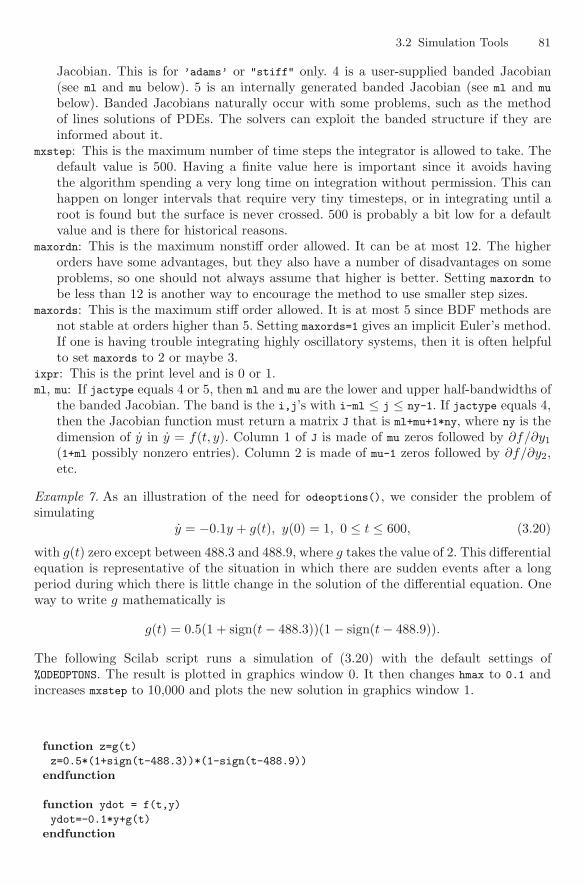
3.2 Simulation Tools 81
Jacobian. This is for ’adams’ or "stiff" only. 4 is a user-supplied banded Jacobian(see ml and mu below). 5 is an internally generated banded Jacobian (see ml and mu
below). Banded Jacobians naturally occur with some problems, such as the methodof lines solutions of PDEs. The solvers can exploit the banded structure if they areinformed about it.
mxstep: This is the maximum number of time steps the integrator is allowed to take. Thedefault value is 500. Having a finite value here is important since it avoids havingthe algorithm spending a very long time on integration without permission. This canhappen on longer intervals that require very tiny timesteps, or in integrating until aroot is found but the surface is never crossed. 500 is probably a bit low for a defaultvalue and is there for historical reasons.
maxordn: This is the maximum nonstiff order allowed. It can be at most 12. The higherorders have some advantages, but they also have a number of disadvantages on someproblems, so one should not always assume that higher is better. Setting maxordn tobe less than 12 is another way to encourage the method to use smaller step sizes.
maxords: This is the maximum stiff order allowed. It is at most 5 since BDF methods arenot stable at orders higher than 5. Setting maxords=1 gives an implicit Euler’s method.If one is having trouble integrating highly oscillatory systems, then it is often helpfulto set maxords to 2 or maybe 3.
ixpr: This is the print level and is 0 or 1.ml, mu: If jactype equals 4 or 5, then ml and mu are the lower and upper half-bandwidths of
the banded Jacobian. The band is the i,j’s with i-ml ≤ j ≤ ny-1. If jactype equals 4,then the Jacobian function must return a matrix J that is ml+mu+1*ny, where ny is thedimension of y in y = f(t, y). Column 1 of J is made of mu zeros followed by ∂f/∂y1
(1+ml possibly nonzero entries). Column 2 is made of mu-1 zeros followed by ∂f/∂y2,etc.
Example 7. As an illustration of the need for odeoptions(), we consider the problem ofsimulating
y = −0.1y + g(t), y(0) = 1, 0 ≤ t ≤ 600, (3.20)
with g(t) zero except between 488.3 and 488.9, where g takes the value of 2. This differentialequation is representative of the situation in which there are sudden events after a longperiod during which there is little change in the solution of the differential equation. Oneway to write g mathematically is
g(t) = 0.5(1 + sign(t − 488.3))(1 − sign(t − 488.9)).
The following Scilab script runs a simulation of (3.20) with the default settings of%ODEOPTONS. The result is plotted in graphics window 0. It then changes hmax to 0.1 andincreases mxstep to 10,000 and plots the new solution in graphics window 1.
function z=g(t)
z=0.5*(1+sign(t-488.3))*(1-sign(t-488.9))
endfunction
function ydot = f(t,y)
ydot=-0.1*y+g(t)
endfunction
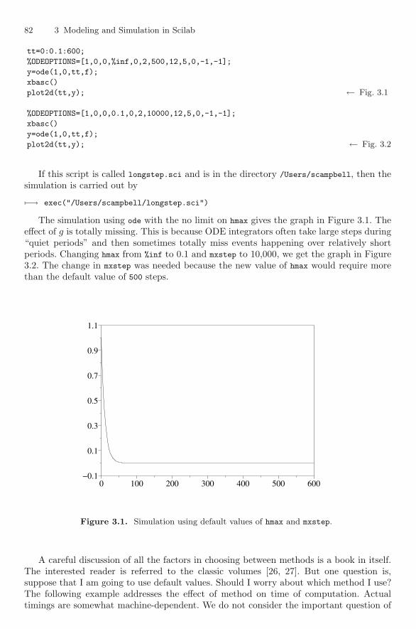
82 3 Modeling and Simulation in Scilab
tt=0:0.1:600;
%ODEOPTIONS=[1,0,0,%inf,0,2,500,12,5,0,-1,-1];
y=ode(1,0,tt,f);
xbasc()
plot2d(tt,y); ← Fig. 3.1
%ODEOPTIONS=[1,0,0,0.1,0,2,10000,12,5,0,-1,-1];
xbasc()
y=ode(1,0,tt,f);
plot2d(tt,y); ← Fig. 3.2
If this script is called longstep.sci and is in the directory /Users/scampbell, then thesimulation is carried out by
�−→ exec("/Users/scampbell/longstep.sci")
The simulation using ode with the no limit on hmax gives the graph in Figure 3.1. Theeffect of g is totally missing. This is because ODE integrators often take large steps during“quiet periods” and then sometimes totally miss events happening over relatively shortperiods. Changing hmax from %inf to 0.1 and mxstep to 10,000, we get the graph in Figure3.2. The change in mxstep was needed because the new value of hmax would require morethan the default value of 500 steps.
0 100 200 300 400 500 600−0.1
0.1
0.3
0.5
0.7
0.9
1.1
Figure 3.1. Simulation using default values of hmax and mxstep.
A careful discussion of all the factors in choosing between methods is a book in itself.The interested reader is referred to the classic volumes [26, 27]. But one question is,suppose that I am going to use default values. Should I worry about which method I use?The following example addresses the effect of method on time of computation. Actualtimings are somewhat machine-dependent. We do not consider the important question of
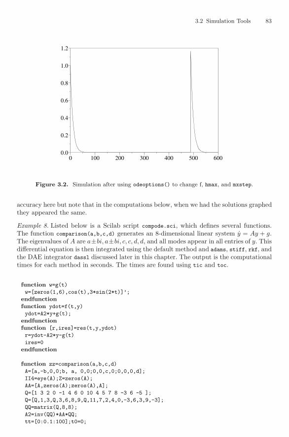
3.2 Simulation Tools 83
0 100 200 300 400 500 6000.0
0.2
0.4
0.6
0.8
1.0
1.2
Figure 3.2. Simulation after using odeoptions() to change f, hmax, and mxstep.
accuracy here but note that in the computations below, when we had the solutions graphedthey appeared the same.
Example 8. Listed below is a Scilab script compode.sci, which defines several functions.The function comparison(a,b,c,d) generates an 8-dimensional linear system y = Ay + g.The eigenvalues of A are a±bi, a±bi, c, c, d, d, and all modes appear in all entries of y. Thisdifferential equation is then integrated using the default method and adams, stiff, rkf, andthe DAE integrator dassl discussed later in this chapter. The output is the computationaltimes for each method in seconds. The times are found using tic and toc.
function w=g(t)
w=[zeros(1,6),cos(t),3*sin(2*t)]’;
endfunctionfunction ydot=f(t,y)
ydot=A2*y+g(t);
endfunctionfunction [r,ires]=res(t,y,ydot)
r=ydot-A2*y-g(t)
ires=0
endfunction
function zz=comparison(a,b,c,d)
A=[a,-b,0,0;b, a, 0,0;0,0,c,0;0,0,0,d];
II4=eye(A);Z=zeros(A);
AA=[A,zeros(A);zeros(A),A];
Q=[1 3 2 0 -1 4 6 0 10 4 5 7 8 -3 6 -5 ];
Q=[Q,1,3,Q,3,6,8,9,Q,11,7,2,4,0,-3,6,3,9,-3];
QQ=matrix(Q,8,8);
A2=inv(QQ)*AA*QQ;
tt=[0:0.1:100];t0=0;
84 3 Modeling and Simulation in Scilab
y0=[1 1 -1 1 2 0 -1 -1 ]’;
ydot0=A2*y0+g(0);
tic;yy1=ode(y0,t0,tt,f);
t1=toc();
tic;yy2=ode("adams",y0,t0,tt,f);
t2=toc();
tic;yy3=ode("stiff",y0,t0,tt,f);
t3=toc();
tic;yy4=ode("rkf",y0,t0,tt,f);
t4=toc();
xstart=[y0,ydot0];
tic;yy5=dassl(xstart,t0,tt,res);
t5=toc();
zz=[t1,t2,t3,t4,t5]
xbasc()
plot2d(tt,yy1(7,:))
plot2d(tt,yy2(7,:))
plot2d(tt,yy3(7,:))
plot2d(tt,yy4(7,:))
plot2d(tt,yy5(8,:))
endfunction
The functions in compode.sci are loaded in Scilab, and to compare the different methodson an easy problem we enter
�−→ comparison(-0.1,2,-3,0.1)
ans =
! 0.318 0.197 0.348 0.525 0.533 !
We see that the methods were comparable, with the Adams method the fastest anddassl the fastest of the stiff methods. Adams is often fastest on problems that are notrapidly varying. rkf is second-best. Generally, Runge–Kutta methods like rkf take morework per time step than a multistep of the same oder such as adams. Also, the adams cango to higher order.
However, some problems, such as those in electrical engineering and some mechanicalsystems can be highly oscillatory. In other areas such as chemical reactions we can havevery rapidly decaying terms. To examine what happens with a rapidly decaying componentwe enter
�−→ comparison(-0.1,2,-5000,0.1)
ans =
! 0.471 2.885 0.422 70.131 0.745 !
We see that the implicit methods default, stiff, and dassl are much faster. adams takes7 times as long as stiff and rkf takes 30 times as long as stiff. The default takes longerthan stiff since it starts as a nonstiff method and then has to switch. As is not unusual,dassl is comparable to stiff but sometimes takes a little longer. That is because dassl isdesigned for fully implicit DAEs and sometimes has to do a bit more work.
3.2 Simulation Tools 85
If a system is highly oscillatory, then some of the methods designed for stiff problemshave to reduce their step size or order for stability reasons. To illustrate, we enter
�−→ comparison(-0.1,100,-3,0.1)
ans =
! 11.787 4.678 8.68 5.793 23.37 !
Whereas in the previous problem the methods of stiff type were clearly faster, we seehere that the stiff methods were much slower. In the case of dassl it has some heuristicsthat look out for oscillatory systems and reduces the order to try to increase stability.
Sometimes simulation is embedded into design or optimization loops so that the samedifferential equations will be integrated many times. As the previous example shows, thecomputational time can vary greatly with the choice of the method. Accuracy can also vary,so that for complex problems one needs to do a careful examination of which integratorwill be fastest and also deliver the desired accuracy.
Implicit Differential Equations
In some application areas the models are most naturally initially formulated as differentialequations in the form
A(t, y)y = g(t, y), y(t0) = y0. (3.21)
If A(t, y) is not invertible for all t, y of interest, then (3.21) is a linear implicit differentialalgebraic equation. If A(y, t) is invertible for all t, y of interest, we call (3.21) either alinearly implicit differential equation or an index-zero DAE. For this section we assumethat A(t, y) is an invertible matrix. One could, of course invert A and get the ODE
y = A(t, y)−1g(t, y) y(t0) = y0. (3.22)
However, this reformulation is not always desirable. The implicit system (3.21) can oftenbe integrated more efficiently and reliably than (3.22). The numerical methods for solving(3.21) are similar to those we discuss later for DAEs of the form F (t, y, y) = 0, whichrequire a way to evaluate F given estimates of y(t), y(t). Traditionally this function F iscalled a residual since iterative numerical methods are used, and when approximations aresubstituted in for y and y, the evaluation of F (t, y, y) tells us how far the approximationsare from being solutions.
One Scilab simulation tool for (3.21) is impl. It is called by
y=impl([type],y0,ydot0,t0,t [,atol, [rtol]],res,adda [,jac])
Most of these variables have the same meaning as they do for ode, but there are someimportant new variables and there are some restrictions on the other variables. If type ispresent, it is either "adams" or "stiff". The algorithm requires an initial value of y(t0)and this is provided in the vector ydot0.
The actual differential equation being integrated enters through the residual res, whichis an external, that is, a function with specified syntax, or the name of a Fortran subroutineor a C function (character string) with specified calling sequence or a list.
If res is a function, its syntax must be r = res(t,y,ydot) and it must return the valueof g(t,y)-A(t,y)*ydot.
86 3 Modeling and Simulation in Scilab
In the implicit methods there are nonlinear equations that must be solved, and theserequire Jacobian information. The variable adda tells the integrator what A is. It also isuseful within the numerical algorithm in setting up other Jacobians. If adda is a function,its syntax must be r = adda(t,y,p) and it must return r=A(t,y)+p, where p is a matrixto be added to A(t,y). As usual, if adda is a character string, it refers to the name of aFortran subroutine or a C function.
The optional input jac is also an external. If jac is a function, it must have the syntaxj = jac(t,y,ydot) and it must return the Jacobian of
r= g(t,y) -A(t,y)*ydot
with respect to y.If a differential equation is fully implicit, that is, F (t, y, y) = 0 with ∂F/∂y nonsingu-
lar, then it is integrated using dassl as described in the section on differential algebraicequations.
Linear Systems
Since they occur so often in areas such as control engineering, there are a number ofspecialized functions for working with linear systems of the form
x = Ax + Bu, (3.23a)y = Cx + Du, (3.23b)
where A, B, C, D are matrices. System (3.23) is called the state-space form. If we letx(0) = 0, take the Laplace transform of (3.23), and let z(s) denote the Laplace transformof z(t), we see that (3.23) can be written as
y(s) = (D + C(sI − A)−1B)u(s) = H(s)u(s), (3.24)
where H is a rational matrix function. That is, the entries of H are fractions of polynomials.Further manipulations would allow us to get
D(s)y(s) = N(s)u(s) = H(s)u(s), (3.25)
where D, N are matrices of polynomials in s.Scilab has functions for working with all three of these ways of describing linear systems.
It also easily switches from one representation to another. Linear systems are defined bythe syslin function. It may be called in three different ways:
[sl]=syslin(dom,A,B,C [,D [,x0] ])
[sl]=syslin(dom,N,D)
[sl]=syslin(dom,H)
The resulting sl is a tlist (“syslin” list) representing the linear system. sl can in turn beused in a number of different Scilab functions. dom is a character string (’c’ , ’d’ , or [] )or a scalar. It defines the domain of the system. ’c’ is for a continuous-time system, ’d’is for a discrete-time system, and a scalar n is for a sampled system with sampling periodn (in seconds). A, B, C, D are the matrices of the state-space representation (3.23). x0 is theinitial state. If x0 is not given, then x0=0. N, D, and H are polynomial and rational matricesrespectively corresponding to (3.25) and (3.24).
If it is desired to recover the values of A, B, C, D, from sl, this is done by the abcd
command,
3.2 Simulation Tools 87
�−→ [A,B,C,D]=abcd(sl)
The scilab command csim provides a simulation using ode of the linear system (3.23)defined by ls. csim is called by
[y [,x]]=csim(u,t,sl,[x0 [,tol]])
u is a function, list, or string that defines the control u. t provides the times requestedfor the simulation values. t(1) is the initial time. y is a matrix of y values such thaty(i)=[y(t(i)] for i = 1, . . . , n. The optional output x is the corresponding values of thestate x. tol is the two-vector [atol rtol] defining absolute and relative error tolerancesfor the ode solver. In addition to the usual choices for u such as a function, list, or vector ofvalues, there are two special options. If u is the string "impuls", then an impulse responsecalculation is done. That is, u is a delta function, or unit impulse, at time t = 0. If u is"impuls", then it is assumed that sl is SISO (single input-single output), D = 0, and x0=0.u can also be "step" for a step response calculation. That is, u = 1 for t > 0. "step" hasthe same assumptions as "impluls".
Example 9. Consider the continuous linear system
x1 = −2x1 + 7x2 + u, (3.26a)x2 = 8x1 − 2x2, (3.26b)y = x1 + x2. (3.26c)
When executed, the following file produces the output for a step input and an impulseinput in two different windows.
A=[-2 7;-8 -2];B=[1;0];C=[1 1 ];D=0;
[sl]=syslin("c",A,B,C);
t=0:0.01:5;
[ys,xs]=csim("step",t,sl); ← Finds step response of systemplot2d(t,ys); ← Fig. 3.3 (upper graph)
[yi,xi]=csim("impuls",t,sl); ← Finds impuls responsef1=scf(1);
xbasc();
plot2d(t,yi) ← Fig. 3.3 (lower graph)
The graphs are given in Figure 3.3.
Root Finding
It is often desirable to simulate a differential equation up to the time something happens.In some cases the time is the quantity of interest, for example in an interception problem.In other cases the time will represent physical change in the dynamics such as when atank is filling up and it starts to overflow. In all these cases we have a system (3.1) and wewish to integrate it until some quantity g(t, y) is equal to 0. Scilab includes root findingsoftware for both ODEs and DAEs. We focus on the ODE case here. The Scilab functionode_root is called by
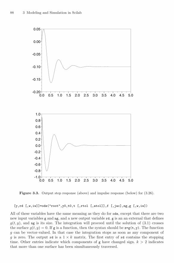
88 3 Modeling and Simulation in Scilab
0.0 0.5 1.0 1.5 2.0 2.5 3.0 3.5 4.0 4.5 5.0-0.20
-0.15
-0.10
-0.05
0.00
0.05
0.0 0.5 1.0 1.5 2.0 2.5 3.0 3.5 4.0 4.5 5.0-1.0
-0.8
-0.6
-0.4
-0.2
0.0
0.2
0.4
0.6
0.8
1.0
Figure 3.3. Output step response (above) and impulse response (below) for (3.26).
[y,rd [,w,iw]]=ode("root",y0,t0,t [,rtol [,atol]],f [,jac],ng,g [,w,iw])
All of these variables have the same meaning as they do for ode, except that there are twonew input variables g and ng, and a new output variable rd. g is an an external that definesg(t, y), and ng is its size. The integration will proceed until the solution of (3.1) crossesthe surface g(t, y) = 0. If g is a function, then the syntax should be z=g(t,y). The functiong can be vector-valued. In that case the integration stops as soon as any component ofg is zero. The output rd is a 1 × k matrix. The first entry of rd contains the stoppingtime. Other entries indicate which components of g have changed sign. k > 2 indicatesthat more than one surface has been simultaneously traversed.
3.2 Simulation Tools 89
It is worth noting that ode_root does not just stop when it crosses the surface g(t, y) =0. Rather, once it has crossed the surface, the algorithm iteratively reduces the last stepin order to try to end on the surface up to the specified tolerances. This is an importantfeature.
When the surface-crossing represents a change in the differential equation, one couldtry to describe this situation using a single function with if statements. However, thenthere is the problem that the numerical simulation will step across the event and makethe change at a later time. Often it is important to have the change occur at the correcttime, and this requires the integrator searching out exactly when the crossing occurs.
Example 10. We suppose that we have a 1,000 cubic meter rectangular tank containingwater that flows out a hole at the bottom. The tank is 10 meters high and initially full.When the tank is three quarters empty, a sensor causes water to be pumped into the tankat a constant rate. We are interested in the amount of water in the tank, which we denoteby V . This may be modeled by V = −c1
√V , V (0) = 1, 000 until V (t) = 250, and then the
differential equation is V = −c1
√V +c2, where c1, c2 are two positive constants determined
by the size of the hole and the pumping rate. We are interested in the first 600 time unitsor until the tank fills back up, whichever occurs first. Listed below is a file tank.sci, whichperforms the simulation. It sets itask to 2 so that all mesh points are output. The if-thenconstruction is built to cover the case in which tf occurs before the surface is reached, whichdoes not happen for the particular flow rates and final time chosen. This implementationalso stops the simulation if the tank fills back up. The simulation is obtained by executingthe next script, and the simulation graph is in Figure 3.4.
function z=f1(t,V) ← tank drainingz=-0.3*sqrt(V);
endfunction
function z=f2(t,V) ← tank draining with pumping inz=-0.3*sqrt(V) +8.0;
endfunction
function z=g(t,V) ← surfacez=250-V;
endfunction
function z=h(t,V) ← end of integrationz=1000-V;
endfunction
%ODEOPTIONS=[2,0,0,%inf,0,2,10000,12,5,0,-1,-1]; ← set itask to 2, increase maxsteptf=600;
[vsol,rd]=ode(’root’,1000,0,tf,f1,1,g);
m=size(vsol);
if rd(1)< tf then[vsol2,rd2]=ode(’root’,vsol(2,m(2)),rd(1),tf,f2,1,h);
sol=[vsol,vsol2];
else sol=vsol;
endxbasc();
plot2d(sol(1,:),sol(2,:)); ← Fig. 3.4
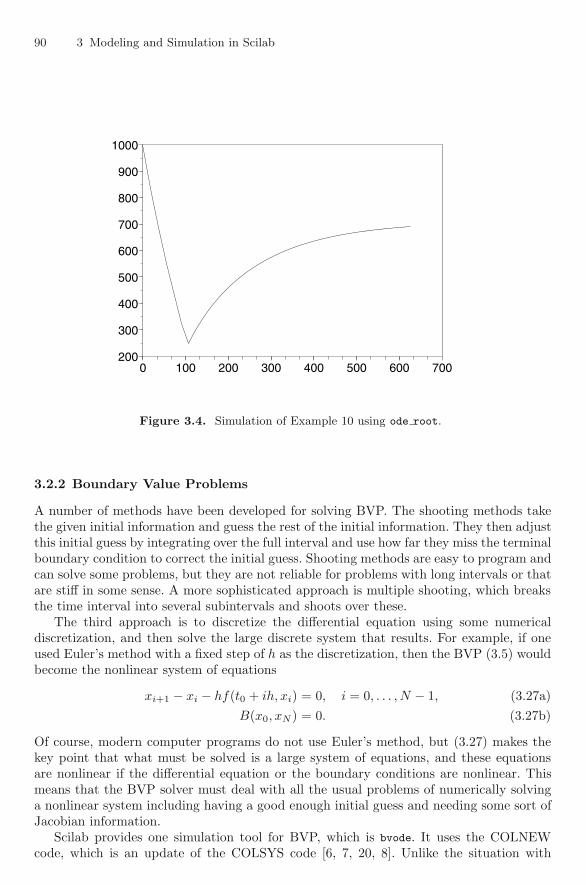
90 3 Modeling and Simulation in Scilab
0 100 200 300 400 500 600 700200
300
400
500
600
700
800
900
1000
Figure 3.4. Simulation of Example 10 using ode root.
3.2.2 Boundary Value Problems
A number of methods have been developed for solving BVP. The shooting methods takethe given initial information and guess the rest of the initial information. They then adjustthis initial guess by integrating over the full interval and use how far they miss the terminalboundary condition to correct the initial guess. Shooting methods are easy to program andcan solve some problems, but they are not reliable for problems with long intervals or thatare stiff in some sense. A more sophisticated approach is multiple shooting, which breaksthe time interval into several subintervals and shoots over these.
The third approach is to discretize the differential equation using some numericaldiscretization, and then solve the large discrete system that results. For example, if oneused Euler’s method with a fixed step of h as the discretization, then the BVP (3.5) wouldbecome the nonlinear system of equations
xi+1 − xi − hf(t0 + ih, xi) = 0, i = 0, . . . , N − 1, (3.27a)B(x0, xN ) = 0. (3.27b)
Of course, modern computer programs do not use Euler’s method, but (3.27) makes thekey point that what must be solved is a large system of equations, and these equationsare nonlinear if the differential equation or the boundary conditions are nonlinear. Thismeans that the BVP solver must deal with all the usual problems of numerically solvinga nonlinear system including having a good enough initial guess and needing some sort ofJacobian information.
Scilab provides one simulation tool for BVP, which is bvode. It uses the COLNEWcode, which is an update of the COLSYS code [6, 7, 20, 8]. Unlike the situation with
3.2 Simulation Tools 91
ode and dassl, which requires the differential equations to be in first-order form, bvode
allows the equations to be of higher order. bvode also allows for boundary conditions atseveral times ζj . It is traditional in parts of the BVP literature to use x instead of t forthe independent variable. We will now switch to that notation.
bvode assumes that the BVP is in the form
dmiui
dx= fi
(x, u(x),
du
dx, . . . ,
dmi−1u
dxmi−1
), 1 ≤ i ≤ nc, (3.28a)
gj
(ζj , u(ζj), . . . ,
dm∗u
dxm∗
)= 0, j = 1, . . . , m∗, (3.28b)
where ζj are the x values where the boundary conditions are to hold and aL ≤ x ≤ aR. Inorder to keep the notation down, let
m∗ = m1 + m2 + · · · + mnc, (3.29)
z(u) =[u,
du
dx, . . . ,
dm∗u
dxm∗
]. (3.30)
Then (3.28) becomes
dmiui
dx= fi(x, z(u(x)), 1 ≤ i ≤ nc, aL ≤ x ≤ aR, (3.31a)
gj(ζj , z(u(ζj)) = 0, j = 1, . . . , m∗. (3.31b)
bvode starts with an initial mesh for the discretization and solves the resulting nonlinearsystem. It then iteratively refines the mesh until either it estimates that the requestedaccuracy has been attained or it reaches the maximum allowable mesh. The call for bvode
takes the form
[z]=bvode(points,ncomp,m,aleft,aright,zeta,ipar,ltol,tol,fixpnt,fsub1,...
dfsub1,gsub1,dgsub1,guess1)
The parameters in the bvode call have the following meanings:
z: The solution of the ode evaluated on the mesh given by points.points: An array that gives the points for which we want the solution.ncomp: The number of differential equations. It must satisfy ncomp ≤ 20.m: A vector of size ncomp . The entry m(j) gives the order of the jth differential equation.
The orders must satisfy m(i) ≤ 4.aleft: The left end of the interval on which u is defined.aright: The right end of the interval on which u is defined.zeta: Entry zeta(j) gives the jth side condition point (boundary point). The entries must
be ordered so that zeta(j) ≤zeta(j+1). All the side (boundary) conditions must be atmesh points in all meshes used. In particular, they must be part of the initial mesh.Note the description of ipar(11) and fixpnt below.
ipar: An integer array with dimension at least 11. A list of the parameters in ipar andtheir meaning follows. Note that some parameters are renamed in bvode. These newnames are given in parentheses.ipar(1): 0 if the problem is linear and 1 if the problem is nonlinear.ipar(2): The number of collocation points per subinterval (= k ) where max m(i) ≤
k ≤ 7. If ipar(2)=0, then bvode sets k = max(maxi m(i) + 1, 5 − maxi m(i)).ipar(3): The number of subintervals in the initial mesh (= n ). If ipar(3) = 0, then
bvode sets n = 5.
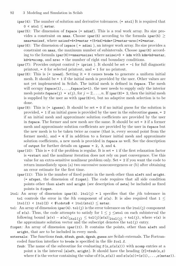
92 3 Modeling and Simulation in Scilab
ipar(4): The number of solution and derivative tolerances. (= ntol) It is required that0 < ntol ≤ mstar.
ipar(5): The dimension of fspace (= ndimf). This is a real work array. Its size pro-vides a constraint on nmax. Choose ipar(5) according to the formula ipar(5) ≥nmax*nsizef, where nsizef=4+3*mstar +(5+kd)*kdm+(2*mstar-nrec)*2*mstar.
ipar(6): The dimension of ispace ( = ndimi ), an integer work array. Its size provides aconstraint on nmax, the maximum number of subintervals. Choose ipar(6) accord-ing to the formula ipar(6)>=nmax*nsizei where nsizei=3 + kdm with kdm=kd+mstar,kd=k*ncomp, and nrec = the number of right end boundary conditions.
ipar(7): Provides output control (= iprint ). It should be set = -1 for full diagnosticprintout, = 0 for selected printout, and = 1 for no printout.
ipar(8): This is (= iread). Setting it = 0 causes bvode to generate a uniform initialmesh. It should be = 1 if the initial mesh is provided by the user. Other values arenot yet implemented in Scilab. The initial mesh is defined in fspace. The meshwill occupy fspace(1),...,fspace(n+1). the user needs to supply only the interiormesh points fspace(j) = x(j), for j = 2, . . . , n. If ipar(8)= 2, then the initial meshis supplied by the user as with ipar(8)=1, but no adaptive mesh selection is to bedone.
ipar(9): This is (= iguess). It should be set = 0 if no initial guess for the solution isprovided, = 1 if an initial guess is provided by the user in the subroutine guess, = 2
if an initial mesh and approximate solution coefficients are provided by the userin fspace. The former and new mesh are the same. It should be set = 3 if a formermesh and approximate solution coefficients are provided by the user in fspace butthe new mesh is to be taken twice as coarse (that is, every second point from theformer mesh), and = 4 if in addition to a former initial mesh and approximatesolution coefficients, a new mesh is provided in fspace as well. See the descriptionof output for further details on iguess = 2, 3, and 4.
ipar(10): This is = 0 if the problem is regular. It is set = 1 if the first relaxation factoris =rstart and the nonlinear iteration does not rely on past convergence. Use thisvalue for an extra-sensitive nonlinear problem only. Set = 2 if you want the code toreturn immediately upon (a) two successive nonconvergences or (b) after obtainingan error estimate for the first time.
ipar(11): This is the number of fixed points in the mesh other than aleft and aright.(= nfxpnt, the dimension of fixpnt). The code requires that all side conditionpoints other than aleft and aright (see description of zeta) be included as fixedpoints in fixpnt.
ltol: An array of dimension ipar(4). ltol(j) = l specifies that the jth tolerance intol controls the error in the lth component of z(u). It is also required that 1 ≤ltol(1) < ltol(2) < $\cdots$ < ltol(ntol) ≤ mstar.
tol: An array of dimension ipar(4). tol(j) is the error tolerance on the ltol(j) componentof z(u). Thus, the code attempts to satisfy for 1 ≤ j ≤ntol on each subinterval thefollowing bound |z(v) − z(u)|ltol(j) ≤ tol(j)|z(u)|ltol(j) + tol(j), where v(x) isthe approximate solution vector and the subscript denotes the tol(j) entry.
fixpnt: An array of dimension ipar(11). It contains the points, other than aleft andaright, that are to be included in every mesh.
externals: The functions fsub, dfsub, gsub, dgsub, guess are Scilab externals. The Fortran-coded function interface to bvode is specified in the file fcol.f.fsub: The name of the subroutine for evaluating f(x,z(u(x))) with ncomp entries at a
point x in the interval (aleft, aright). It should have the heading [f]=fsub(x,z)
where f is the vector containing the value of f(x,z(u)) and z(u(x))=(z(1),...,z(mstar)).
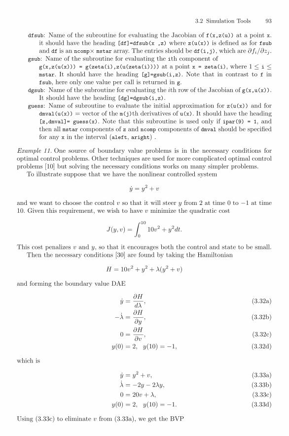
3.2 Simulation Tools 93
dfsub: Name of the subroutine for evaluating the Jacobian of f(x,z(u)) at a point x.it should have the heading [df]=dfsub(x ,z) where z(u(x)) is defined as for fsub
and df is an ncomp× mstar array. The entries should be df(i,j), which are ∂fi/∂zj .gsub: Name of the subroutine for evaluating the ith component of
g(x,z(u(x))) = g(zeta(i),z(u(zeta(i)))) at a point x = zeta(i), where 1 ≤ i ≤mstar. It should have the heading [g]=gsub(i,z). Note that in contrast to f infsub, here only one value per call is returned in g.
dgsub: Name of the subroutine for evaluating the ith row of the Jacobian of g(x,u(x)).It should have the heading [dg]=dgsub(i,z).
guess: Name of subroutine to evaluate the initial approximation for z(u(x)) and fordmval(u(x)) = vector of the m(j)th derivatives of u(x). It should have the heading[z,dmval]= guess(x). Note that this subroutine is used only if ipar(9) = 1, andthen all mstar components of z and ncomp components of dmval should be specifiedfor any x in the interval (aleft, aright) .
Example 11. One source of boundary value problems is in the necessary conditions foroptimal control problems. Other techniques are used for more complicated optimal controlproblems [10] but solving the necessary conditions works on many simpler problems.
To illustrate suppose that we have the nonlinear controlled system
y = y2 + v
and we want to choose the control v so that it will steer y from 2 at time 0 to −1 at time10. Given this requirement, we wish to have v minimize the quadratic cost
J(y, v) =∫ 10
0
10v2 + y2dt.
This cost penalizes v and y, so that it encourages both the control and state to be small.Then the necessary conditions [30] are found by taking the Hamiltonian
H = 10v2 + y2 + λ(y2 + v)
and forming the boundary value DAE
y =∂H
dλ, (3.32a)
−λ =∂H
∂y, (3.32b)
0 =∂H
∂v, (3.32c)
y(0) = 2, y(10) = −1, (3.32d)
which is
y = y2 + v, (3.33a)λ = −2y − 2λy, (3.33b)0 = 20v + λ, (3.33c)
y(0) = 2, y(10) = −1. (3.33d)
Using (3.33c) to eliminate v from (3.33a), we get the BVP

94 3 Modeling and Simulation in Scilab
y = y2 − λ/20, (3.34a)λ = −2y − 2λy, (3.34b)
y(0) = 2, y(10) = −1. (3.34c)
We will now solve the BVP using bvode. To simplify things, we shall use the defaultswhenever possible. In particular, we will not provide Jacobians or an initial guess. Thefollowing script sets up all the needed values for the call. A dummy guess is included sincethe call requires something in the guess position even if not used. After the BVP is solvedthe optimal y(t) and v(t) are plotted on the same graph as shown in Figure 3.5. The solidline is y(t) and the x-line curve plots v(t). In this problem the origin is unstable. Thecontrol has to work harder to get the solution near zero at the start than it does at theend of the interval.
function w=f(x,z)
w1=z(1)^2-z(2)/20;
w2=-2*z(1)-2*z(1)*z(2)
w=[w1;w2];
endfunction
function w=df(x,z)
w=[2*z(1),-1/20;-2-2*z(2),-2*z(1)]
endfunction
function w=g(i,z)
if i==1 then w=z(1)-2,
else w=z(1)+1;
endendfunction
function w=dg(i,z)
w=[1 0]
endfunction
tt=0:0.1:10;
ncomp=2;nrec=1;
m=[1 1];k=4; ← k=4 since ipar(2)=0 belownmax=200; ← set the maximum number of subintervals
mstar=2; ← begin computation for ipar(5), ipar(6)kd=k*ncomp;
kdm=kd+mstar;
nsizei=kdm+3;
ip6=nmax*nsizei;
nsizef=4+3*mstar+(5+kd)*kdm+(2*mstar-nrec)*2*mstar;
ip5=nmax*nsizef;
zeta=[0 10]; ← aleft=0 and aright=10
ipar=[1 0 0 2, ip5, ip6, 0 0 0 0 0];
er=1.0d-3;
ltol=[1 1];
tol=[er,er];
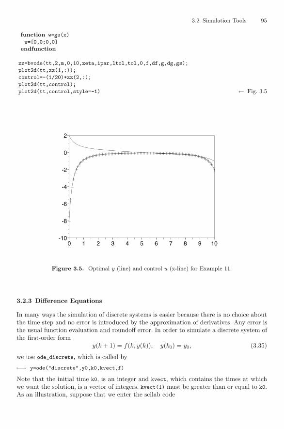
3.2 Simulation Tools 95
function w=gs(x)
w=[0,0;0,0]
endfunction
zz=bvode(tt,2,m,0,10,zeta,ipar,ltol,tol,0,f,df,g,dg,gs);
plot2d(tt,zz(1,:));
control=-(1/20)*zz(2,:);
plot2d(tt,control);
plot2d(tt,control,style=-1) ← Fig. 3.5
0 1 2 3 4 5 6 7 8 9 10-10
-8
-6
-4
-2
0
2
Figure 3.5. Optimal y (line) and control u (x-line) for Example 11.
3.2.3 Difference Equations
In many ways the simulation of discrete systems is easier because there is no choice aboutthe time step and no error is introduced by the approximation of derivatives. Any error isthe usual function evaluation and roundoff error. In order to simulate a discrete system ofthe first-order form
y(k + 1) = f(k, y(k)), y(k0) = y0, (3.35)
we use ode_discrete, which is called by
�−→ y=ode("discrete",y0,k0,kvect,f)
Note that the initial time k0, is an integer and kvect, which contains the times at whichwe want the solution, is a vector of integers. kvect(1) must be greater than or equal to k0.As an illustration, suppose that we enter the scilab code
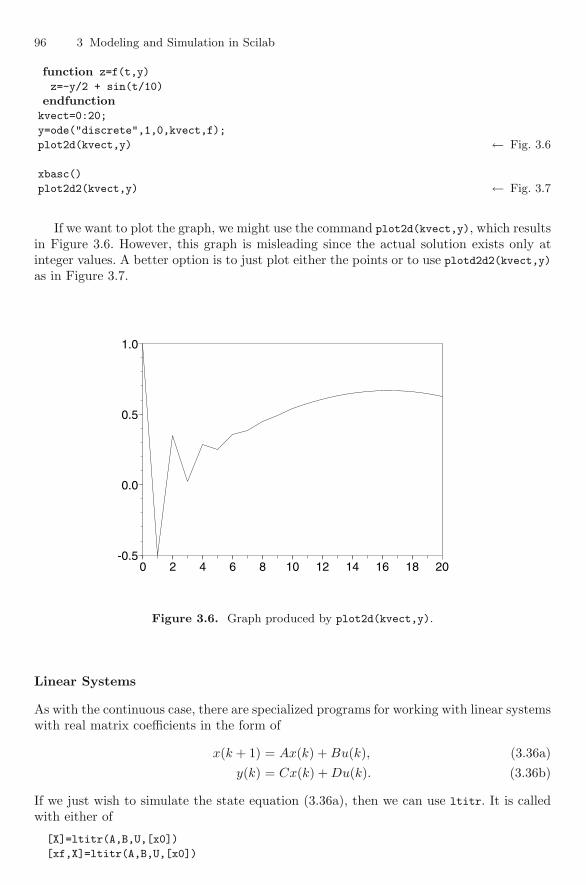
96 3 Modeling and Simulation in Scilab
function z=f(t,y)
z=-y/2 + sin(t/10)
endfunctionkvect=0:20;
y=ode("discrete",1,0,kvect,f);
plot2d(kvect,y) ← Fig. 3.6
xbasc()
plot2d2(kvect,y) ← Fig. 3.7
If we want to plot the graph, we might use the command plot2d(kvect,y), which resultsin Figure 3.6. However, this graph is misleading since the actual solution exists only atinteger values. A better option is to just plot either the points or to use plotd2d2(kvect,y)
as in Figure 3.7.
0 2 4 6 8 10 12 14 16 18 20-0.5
0.0
0.5
1.0
Figure 3.6. Graph produced by plot2d(kvect,y).
Linear Systems
As with the continuous case, there are specialized programs for working with linear systemswith real matrix coefficients in the form of
x(k + 1) = Ax(k) + Bu(k), (3.36a)y(k) = Cx(k) + Du(k). (3.36b)
If we just wish to simulate the state equation (3.36a), then we can use ltitr. It is calledwith either of
[X]=ltitr(A,B,U,[x0])
[xf,X]=ltitr(A,B,U,[x0])
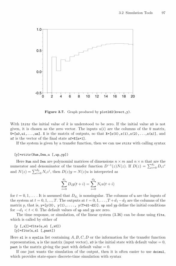
3.2 Simulation Tools 97
0 2 4 6 8 10 12 14 16 18 20-0.5
0.0
0.5
1.0
Figure 3.7. Graph produced by plot2d2(kvect,y).
With ltitr the initial value of k is understood to be zero. If the initial value x0 is notgiven, it is chosen as the zero vector. The inputs u(i) are the columns of the U matrix,U=[u0,u1,...,un]. X is the matrix of outputs, so that X=[x(0),x(1),x(2),...,x(n)], andxf is the vector of the final state xf=X[n+1].
If the system is given by a transfer function, then we can use rtitr with calling syntax
[y]=rtitr(Num,Den,u [,up,yp])
Here Num and Den are polynomial matrices of dimensions n×m and n× n that are thenumerator and denominator of the transfer function D−1(z)N(z). If D(z) =
∑d1i=0 Diz
i
and N(z) =∑d2
i=0 Nizi, then D(z)y = N(z)u is interpreted as
d1∑i=0
Diy(t + i) =d2∑
i=0
Niu(t + i)
for t = 0, 1, . . . . It is assumed that Dd1 is nonsingular. The columns of u are the inputs ofthe system at t = 0, 1, ..., T . The outputs at t = 0, 1, . . . , T +d1−d2 are the columns of thematrix y, that is, y=[y(0), y(1),...., y(T+d1-d2)]. up and yp define the initial conditionsfor −d1 < t < 0. The default values of up and yp are zero.
The time response, or simulation, of the linear system (3.36) can be done using flts,which is called by either of
[y [,x]]=flts(u,sl [,x0])
[y]=flts(u,sl [,past])
Here sl is a syslin list containing A, B, C, D or the information for the transfer functionrepresentation, u is the matrix (input vector), x0 is the initial state with default value = 0,past is the matrix giving the past with default value = 0.
If one just wants the simulation of the output, then it is often easier to use dsimul,which provides state-space discrete-time simulation with syntax
98 3 Modeling and Simulation in Scilab
y=dsimul(sl,u)
If [A,B,C,D]=abcd(sl) and x0=sl(’X0’), then dsimul returns
y=C*ltitr(A,B,u,x0)+D*u.
With dsimul it is assumed that sl is in state-space form.
3.2.4 Differential Algebraic Equations
Before giving the simulation tools for DAEs it is helpful first to point out some of therequirements of these tools. With an ODE one had only to supply the initial value of y(t0).But a DAE needs information on both y(t0) and y(t0) in order to uniquely determine thesolution and get the integration started. Consider, for example, the implicit ODE tan(y) =−y + g(t). This actually defines a family of differential equations y = tan−1(y + g) + nπ.Without a value for y, the integrator would not be able to determine which family it shouldbe integrating. There are a number of possibilities. A user might have a value of y. Or onemay have only an approximate value. Sometimes one has no idea at all. We return to thisproblem in Example 12.
The simulation tools in Scilab use backward differentiation formulas (BDF). For ex-ample, a backward Euler’s method applied to (3.15) would take the form
F
(tn+1.yn+1,
yn+1 − yn
h
)= 0. (3.37)
Given yn, equation (3.37) must be solved by an iterative method. The Jacaobian withrespect to yn+1 of (3.37) is Fy + 1
hFy′ . This accounts for the different form that the inputjac has in dassl below from what it had in some of the earlier simulation tools.
Scilab provides the DAE simulation tool dassl, which is the DASSL code developedby Linda Petzold [11]. DASSL integrates general nonlinear fully implicit index-one DAEs.It can also be used on implicit ODEs. DASSL is called by
[r [,hd]]=dassl(x0,t0,t [,atol,[rtol]],res [,jac] [,info] [,hd])
If y is n-dimensional, then r will have 2n + 1 rows. The first row is the returnedvalues of t. The next n rows are the corresponding values of y, and the last n rows arethe corresponding values of y. info is a list that passes information on to DASSL thatis specific to the solution of index-one DAEs. It also provides some of the informationprovided by %ODEOPTIONS for ode. It will be described more carefully below.
The inputs to dassl have the following meanings:
x0: This can can be either y0, in which case ydot0 is estimated by dassl with zero as itsfirst estimate of ydot0, or x0 can be the matrix [y0, ydot0]. If ydot0 is provided, thenF(t,y0,ydot0) must be equal to zero. If you know only an estimate of ydot0, then setinfo(7)=1.
t0: This is the initial time.t: As with ode, the vector t gives the times that the solution is outputted. If you want
the solution at every time step, then set info(2)=1.atol, rtol: As with ode, atol and rtol are real scalars or column vectors of the same size
as y giving the absolute and relative error tolerances requested of the solution.res: This is an external as with impl. res computes the value of F(t,y,ydot). If res is a
function, its calling sequence must be [r,ires]=res(t,y,ydot). res must return theresidue r=g(t,y,ydot) and an error flag ires. ires = 0 if res succeeds in computingr. ires =-1 if the residue is not defined for the given values of (t,y,ydot). ires =-2 ifthe parameters are out of the admissible range.
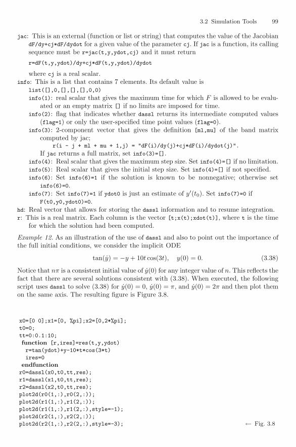
3.2 Simulation Tools 99
jac: This is an external (function or list or string) that computes the value of the JacobiandF/dy+cj*dF/dydot for a given value of the parameter cj. If jac is a function, its callingsequence must be r=jac(t,y,ydot,cj) and it must return
r=dF(t,y,ydot)/dy+cj*dF(t,y,ydot)/dydot
where cj is a real scalar.info: This is a list that contains 7 elements. Its default value is
list([],0,[],[],[],0,0)
info(1): real scalar that gives the maximum time for which F is allowed to be evalu-ated or an empty matrix [] if no limits are imposed for time.
info(2): flag that indicates whether dassl returns its intermediate computed values(flag=1) or only the user-specified time point values (flag=0).
info(3): 2-component vector that gives the definition [ml,mu] of the band matrixcomputed by jac;
r(i - j + ml + mu + 1,j) = "dF(i)/dy(j)+cj*dF(i)/dydot(j)".
If jac returns a full matrix, set info(3)=[].info(4): Real scalar that gives the maximum step size. Set info(4)=[] if no limitation.info(5): Real scalar that gives the initial step size. Set info(4)=[] if not specified.info(6): Set info(6)=1 if the solution is known to be nonnegative; otherwise set
info(6)=0.info(7): Set info(7)=1 if ydot0 is just an estimate of y′(t0). Set info(7)=0 if
F(t0,y0,ydot0)=0.hd: Real vector that allows for storing the dassl information and to resume integration.r: This is a real matrix. Each column is the vector [t;x(t);xdot(t)], where t is the time
for which the solution had been computed.
Example 12. As an illustration of the use of dassl and also to point out the importance ofthe full initial conditions, we consider the implicit ODE
tan(y) = −y + 10t cos(3t), y(0) = 0. (3.38)
Notice that nπ is a consistent initial value of y(0) for any integer value of n. This reflects thefact that there are several solutions consistent with (3.38). When executed, the followingscript uses dassl to solve (3.38) for y(0) = 0, y(0) = π, and y(0) = 2π and then plot themon the same axis. The resulting figure is Figure 3.8.
x0=[0 0];x1=[0, %pi];x2=[0,2*%pi];
t0=0;
tt=0:0.1:10;
function [r,ires]=res(t,y,ydot)
r=tan(ydot)+y-10*t*cos(3*t)
ires=0
endfunctionr0=dassl(x0,t0,tt,res);
r1=dassl(x1,t0,tt,res);
r2=dassl(x2,t0,tt,res);
plot2d(r0(1,:),r0(2,:));
plot2d(r1(1,:),r1(2,:));
plot2d(r1(1,:),r1(2,:),style=-1);
plot2d(r2(1,:),r2(2,:));
plot2d(r2(1,:),r2(2,:),style=-3); ← Fig. 3.8
100 3 Modeling and Simulation in Scilab
0 1 2 3 4 5 6 7 8 9 10-10
0
10
20
30
40
50
60
Figure 3.8. Simulation of (3.38) using dassl for three values of y(0).
The fact that implicit ODEs and fully implicit DAEs can have multiple nearby solu-tions for the same value of the state has important consequences for the design of theseintegrators since this behavior shows up in applications. The integrators must try to ensurethat when making a step they do not jump to another solution. This is accomplished bybeing conservative in choosing the size of the step.
DAEs and Root-Finding
Root-finding with DAEs is done with dasrt, which is dassl along with the ability to findwhere the solution of the DAE crosses a surface. The calling sequence for dasrt is the sameas for dassl except for two inputs, which are the same as for ode using the type “root.”The calling sequence of dasrt is
[r,nn,[,hd]]=dasrt(x0,t0,t [,atol,[rtol]],res [,jac],ng, surf [,info] [,hd])
The differences from the calling of dassl are nn, which is a vector with two entries[times num]. times is the value of the time at which the surface is crossed, and num is thenumber of the crossed surface. surf is an external (function or list or string) that computesthe value of the column vector surf(t,y) with ng components. Each component defines asurface. If surf is a function, its calling sequence must be surf(t,y).
3.2.5 Hybrid Systems
Many systems have both continuous-time and discrete-time components. The simulationtool odedc is designed to integrate some of these models. It is assumed that there arecontinuous variables yc and discrete variables yd that can change at discrete times tk. yd
is considered as a function of continuous time by making it piecewise constant on theintervals [tk, tk+1[.
The system that is integrated then takes the form
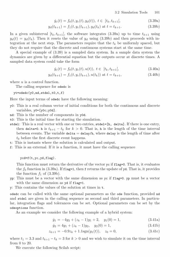
3.2 Simulation Tools 101
yc(t) = f0(t, yc(t), yd(t)), t ∈ [tk, tk+1[, (3.39a)yd(tk+1) = f1(t, yc(tk+1), yd(tk) at t = tk+1. (3.39b)
In a given subinterval [tk, tk+1], the software integrates (3.39a) up to time tk+1 usingyd(t) = yd(tk). Then it resets the value of yd using (3.39b) and then proceeds with in-tegration at the next step. The parameters require that the tk be uniformly spaced, butthey do not require that the discrete and continuous systems start at the same time.
A special example of (3.39) is a sampled data system. In a sample data system thedynamics are given by a differential equation but the outputs occur at discrete times. Asampled data system could take the form
yc(t) = f0(t, yc(t), u(t)), t ∈ [tk, tk+1[, (3.40a)yd(tk+1) = f1(t, yc(tk+1), u(tk)) at t = tk+1, (3.40b)
where u is a control function.The calling sequence for odedc is
yt=odedc(y0,nd,stdel,t0,t,f)
Here the input terms of odedc have the following meaning:
y0: This is a real column vector of initial conditions for both the continuous and discretevariables, y0=[y0c;y0d].
nd: This is the number of components in y0d.t0: This is the initial time for starting the simulation.stdel: This is a real vector with one or two entries, stdel=[h, delta]. If there is one entry,
then delta=0. h is tk+1 − tk for k > 0. That is, h is the length of the time intervalbetween events. The variable delta = delay/h, where delay is the length of time aftert0 before the first discrete event happens.
t: This is instants where the solution is calculated and output.f: This is an external. If it is a function, it must have the calling sequence
ycd=f(t,yc,yd,flag).
This function must return the derivative of the vector yc if flag=0. That is, it evaluatesthe f0 function in (3.39a). If flag=1, then f returns the update of yd. That is, it providesthe function f1 of (3.39b).
yp: This must be a vector with the same dimension as yc if flag=0. yp must be a vectorwith the same dimension as yd if flag=1.
y: This contains the values of the solution at times in t.
odedc can be called with the same optional parameters as the ode function, provided nd
and stdel are given in the calling sequence as second and third parameters. In particu-lar, integration flags and tolerances can be set. Optional parameters can be set by theodeoptions function.
As an example we consider the following example of a hybrid system:
y1 = −4y2 + (zk − 1)y1 + 2, y1(0) = 1, (3.41a)y2 = 4y1 + (zk − 1)y2, y2(0) = 1, (3.41b)
zk+1 = −0.9zk + 1.1sgn(y1(t)), z0 = 0, (3.41c)
where t1 = 3.3 and tk+1 − tk = 3 for k > 0 and we wish to simulate it on the time intervalfrom 0 to 20.
We execute the following Scilab script:
102 3 Modeling and Simulation in Scilab
function ycd=f(t,yc,yd,flag)
if flag==0 thenycd(1)= -4*yc(2)+(yd-1)*yc(1) + 2;
ycd(2)=4*yc(1)+(yd-1)*yc(2);
elseycd=-0.9*yd+ 1.1*sign(yc(1));
endendfunction
t0=0;y0=[1;1;0];nd=1;stdel=[3 1.1];
tt=0:0.1:20;
yt=odedc(y0,nd,stdel,t0,tt,f);
xbasc();
plot2d(tt’,yt’); ← Fig. 3.9
The result is the plot of the three components in Fig. 3.9. The graph of yd is given bythe square wave form. The two components of yc are the wiggly curves that change theirbehavior each time that yd changes.
0 2 4 6 8 10 12 14 16 18 20-0.6
-0.4
-0.2
0.0
0.2
0.4
0.6
0.8
1.0
1.2
1.4
Figure 3.9. Simulation of (3.41) using odedc.
We conclude with an example of a sampled data system.
Example 13. Suppose that we have started with the linear system
x =(
0.1 −11 0.1
)x +
(10
)u. (3.42)
This system is unstable. A feedback control
3.2 Simulation Tools 103
u =(−2 −1
)x (3.43)
is designed to stabilize the system. The control is to be applied starting at time t = 15.Sometimes it is possible to measure the state at any time, but suppose that we are onlyable to determine the state every ρ time units starting at time t = 5. The following scriptwhen executed performs three simulations. The first is using the continuous version of thecontrol. The second and third are with ρ = 1 and ρ = 0.9.
Figure 3.10 shows the effect of the continuous-time feedback. Once the feedback isapplied at t = 15 it quickly stabilizes the system. If the sampling is rapid enough, theresult is essentially the same as using the continuous feedback. However, as Figure 3.11shows, once the sampling period is ρ = 0.9, the system is still stabilized, but it takes muchlonger for the state to go to zero. Once the sampling period reaches 1, the control no longerstabilizes the system, as shown in Figure 3.12.
function z=control(t,x)
if t<15 then z=0,
else z=-2*x(1)-x(2);
endendfunction
function xdot =f(t,x)
xdot=[.1 -1;10.1]*x +[control(t,x);0]
endfunction
x0=[1;1];
tt=[0:0.1:40];
y=ode(x0,0,tt,f);
xbasc();
plot2d(tt,y(1,:)); ← Fig. 3.10
xbasc()
xd0=[1;1];
xc0=[0;0];
function ycd =fcd(t,yc,yd,flag)
if flag==0 then ycd=[.1 -1;10.1]*yc +[control(t,yd);0],
else ycd=yc;
endendfunction
yy=odedc([xd0;xc0],2,[1,5],0,tt,fcd);
plot2d(tt,yy(1,:)); ← Fig. 3.12
xbasc()
yy=odedc([xd0;xc0],2,[0.9,5/0.9],0,tt,fcd);
plot2d(tt,yy(1,:)); ← Fig. 3.11
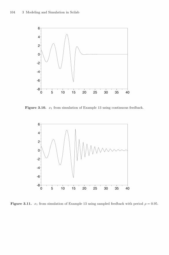
104 3 Modeling and Simulation in Scilab
0 5 10 15 20 25 30 35 40-8
-6
-4
-2
0
2
4
6
Figure 3.10. x1 from simulation of Example 13 using continuous feedback.
0 5 10 15 20 25 30 35 40-8
-6
-4
-2
0
2
4
6
Figure 3.11. x1 from simulation of Example 13 using sampled feedback with period ρ = 0.95.
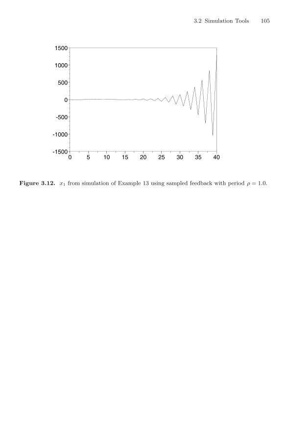
3.2 Simulation Tools 105
0 5 10 15 20 25 30 35 40-1500
-1000
-500
0
500
1000
1500
Figure 3.12. x1 from simulation of Example 13 using sampled feedback with period ρ = 1.0.
4
Optimization
Various optimization problems play a fundamental role in modeling and simulation. Thischapter will cover some of the optimization utilities available in Scilab. Section 4.1 willpresent some overview comments about optimization, useful in using the algorithms. Sec-tion 4.2 discusses the most general optimization utilities. There is a close relationshipbetween optimization and solving equations in a least squares sense. This is examined inSection 4.4. One application of optimization is parameter fitting. Specialized utilities forthis are given in Section 4.5. Finally, some specialized optimization utilities for linear andquadratic programming are given in Section 4.6.
4.1 Comments on Optimization and Solving Nonlinear Equations
In this chapter we discuss the problem of solving the minimization problem
minx
f(x), (4.1)
where f is a real-valued function of the vector variable x. Note that maximizing f isthe same as minimizing −f , so that all of the utilities given here can also be used withmaximization problems.
There are a number of characteristics of (4.1) that determine which, of any, of theavailable utilities will work. They also affect how the optional parameters should be set ifa simple call does not work.
Constraints
The first question is whether there are any restrictions on x (4.1). if there are, the problemis said to be constrained. As far as Scilab is concerned there are three types of constraints.
Bound, or box, constraints require different entries of x to lie in specified intervals.For example, if x is 3 dimensional, we could have −2 ≤ x(1) ≤ 3 and 2 ≤ x(3) ≤ 4.
Linear equality constraints take the form of b′x − c = 0 when b and x are writtenas column vectors. Linear inequality constraints take the form b′x − c ≤ 0 when b, x arewritten as column vectors.
Finally there are the more general constraints of the form g(x) = 0. There are notcurrently any utilities in Scilab for solving general constrained optimal control problems.However, if the problem takes the form
108 4 Optimization
minx f(x), (4.2a)g(x) = 0, (4.2b)
and f, g are differentiable, then the solution x∗ of (4.2) satisfies the necessary conditions
fx(x) + λT gx(x) = 0, (4.3a)g(x) = 0, (4.3b)
where gx is the Jacobian of g, which is discussed below.It is sometimes possible to solve (4.3) using fsolve as discussed later in this chapter.The next question is whether f is a differentiable function and whether we know what
its gradient is. If f is differentiable, then often some type of iterative method is used. Insidethe iterative method at each iteration there is the determination of a search direction anda decision on how far to move in that direction. Then there are questions of how longthe iteration will continue. Common choices are until f does not change much, until thegradient of f is small, or when the allowed number of iterations has been used. The lastcriterion can be important if function evaluations are computationally expensive.
These types of iterative methods, when they find a minimum, usually find local minima.That is, they find where f is smaller than at nearby values. Such local minima may ormay not be a global minimum, that is, the place where f is smallest for all possible x.
A different type of algorithm is sometimes called a “dart-throwing algorithm.” Thesealgorithms vary in philosophy, but basically they continue to evaluate throughout theregion but take more values where the function appears small. While usually much slowerthan iterative methods when both can be used, the dart-throwing algorithms are more aptto find a global minimum and multiple minimum values.
Nonlinear Equation Solving
A nonlinear equation takes the form
f(x) = 0. (4.4)
In the simplest case this represents n equations in n unknowns. Such equations are alsosolved by iterative methods. A key role is played by the Jacobian matrix J(x). If f has mentries and x has n entries, then
J(x) =
⎛⎜⎝
∂f1∂x1
· · · ∂f1∂xn
.... . .
...∂fm
∂x1· · · ∂fm
∂xn
⎞⎟⎠ .
When m = n, and J(x) is invertible, the simplest iterative method is Newton’s method,which is
xj+1 = xj − J(xj)−1f(xj).
Actual solvers utilize a number of methods to increase the region of convergence and toprovide estimates of J .
4.2 General Optimization
The general optimization utility in Scilab is optim. This algorithm allows the user to havesome control of the optimization process. It can accept bound constraints. optim needs to
4.2 General Optimization 109
know the gradient. If the gradient is unknown, or too complicated to code, then a utility isprovided to enable optim to proceed using only the function to be minimized. This utility isNDcost, which stands for numerical differentiation of the cost. It approximates the gradientusing finite differences.
There are additional software programs whose distribution is maintained by the de-veloper but for which there exist Scilab interfaces. For example, a toolbox providing aninterface for the general optimization code can be found at http://www.scilab.org/under contributions, and then downloads, in the category “Optimization Tools.” In par-ticular, there is an interface to FSQP that can handle more general types of constraintsthan optim can.
We shall first present the simplified use of optim and NDcost. We will then discuss someof the more general options. The simplified call is
�−→ [f,xopt]=optim(costf,x0)
Here x0 is the initial guess for where the minimum occurs, f is the optimum value, andxopt is where this optimum value occurs. costf is a function that provides the value ofthe function to be minimized, the value of its gradient, and a variable that is used by theoptimization routine that we will explain later. If costf is a Scilab function, it takes theform
�−→ [f,g,ind]=costf(x,ind)
Of course, for a more complicated problem we may not be able to, or prefer not to,provide the gradient. Then we can use the NDcost function. In its simplest form the callto optim then takes the form
�−→ [f,xopt]=optim(list(NDcost,myf),x0)
In using optim and providing the gradient, the initial guess x0 can be either a row orcolumn and then the xopt will be the same. However, in using NDcost, the initial guessmust be a column vector.
Suppose that we wished to minimize the function
f(x, y, z) = (x − z)2 + 3(x + y + z − 1)2 + (x − z + 1)2. (4.5)
Its gradient is
∇f =[∂f
∂x,∂f
∂y,∂f
∂z
]= [2(x − z) + 6(x + y + z − 1) + 2(x − z + 1), 6(x + y + z − 1),
−2(x − z + 1) + 6(x + y + z − 1)] , (4.6)
and we take an initial guess of x0 = [0, 0, 0]. The following script solves using the gradientand then solves the problem using optim.
function z= myf(x)
z=(x(1)-x(3))^2+3*(x(1)+x(2)+x(3)-1)^2+(x(1)-x(3)+1)^2
endfunction
function z=myg(x)
xs=x(1)+x(2)+x(3)-1;
z=[2*(x(1)-x(3))+6*xs+2*(x(1)-x(3)+1), 6*xs,...
-2*(x(1)-x(3))+6*xs-2*(x(1)-x(3)+1)]

110 4 Optimization
endfunction
function [f,g,ind]=costf(x,ind)
f=myf(x);g=myg(x);
endfunction
x0=[0 0 0]; ← initial condition[fopt,xopt]=optim(costf,x0); ← x0 a row vector[fopt,xopt]=optim(costf,x0’); ← x0 a column vector[fopt,xopt,gopt]=optim(list(NDcost,myf),x0’); ← x0 must be a column
When executed, after listing the function definitions, the output gives the results:
�−→ x0=[0 0 0]; ← initial condition�−→ [fopt,xopt]=optim(costf,x0) ← x0 a row vectorxopt =
! 0.0833333 0.3333333 0.5833333 !
fopt =
0.5
�−→ [fopt,xopt]=optim(costf,x0’) ← x0 a column vectorxopt =
! 0.0833333 !
! 0.3333333 !
! 0.5833333 !
fopt =
0.5
�−→ [fopt,xopt,gopt]=optim(list(NDcost,myf),x0’) ← x0 must be a columngopt =
! 0. !
! 0. !
! - 1.833D-11 !
xopt =
! 0.0833333 !
! 0.3333333 !
! 0.5833333 !
fopt =
0.5
In more complicated problems the user often has to set limits on how many iterationsare taken in order to control the time of computation. In these cases the value of thegradient is very useful information, since if we are at a local optimum of an unconstrainedsmooth problem, then the gradient should be zero. Note that in the NDcost we get anumerical estimate of the gradient and it is close to zero. Requesting the value of thegradient at the optimal point is a general option with optim, as we will now show.
4.2 General Optimization 111
For more complicated problems, the user will want to use some of the options of optim,which we will now describe. The full calling format is
[f,[xopt,[gradopt,[work]]]]=optim(costf,[contr],x0,[’algo’],....
[df0,[mem]],[work],[stop],[’in’],[imp=iflag])
These parameters are as follows. Using some of them requires knowledge about the iterativenumerical methods used.
• costf: An external, Scilab function, list, or string (costf is the cost function: see itscalling sequence below (Scilab, C, or Fortran)). x0: real vector (initial value of variableto be minimized).
• f: Value of optimal cost.• xopt: Best value of x found.• contr: The three entries ’b’,binf,bsup. binf and bsup are real vectors with the same
dimension as x0. binf and bsup are lower and upper bounds on x.• "algo": Determines the algorithm. ’qn’ is quasi-Newton, which is the default. ’gc’
is conjugate gradient. ’nd’ stands for nondifferentiable. Use this if there are pointswhere the cost function does not have a derivative. An example is abs, which is notdifferentiable at zero. Note that ’nd’ does not accept bounds on x.
• df0: Real scalar giving the guessed decrease of f at first iteration. df0=1 is the defaultvalue. It affects the efficiency of the line-search algorithm.
• mem: An integer giving number of variables used to approximate the Hessian whenalgo=’gc’ or ’nd’. Default value is around 6.
• stop: A sequence of optional parameters controlling the convergence of the algorithm.stop= ’ar’,nap, [iter [,epsg [,epsf [,epsx]]]], where– "ar": Reserved keyword for stopping rule selection defined as follows:– nap: Maximum number of calls to costf allowed.– iter: Maximum number of iterations allowed.– epsg: Threshold on gradient norm.– epsf: Threshold controlling decreasing of f.– epsx: Threshold controlling variation of x. This vector (possibly matrix) of same
size as x0, can be used to scale x.• "in": Reserved keyword for initialization of parameters used when costf is given as a
C or Fortran routine.• "imp=iflag": Named argument used to set the trace mode. If iflag=0, then nothing
except errors are reported. If iflag=1, then there are initial and final reports. If iflag=2,then there is an additional report per iteration. iflag>2 adds reports on linear search.Most of these reports are written on the Scilab standard output, so if there are manyiterations involving vectors, there could be a lot of output.
• gradopt: Gradient of costf at xopt.• work: Working array for hot restart for quasi-Newton method. This array is automati-
cally initialized by optim when optim is invoked. It can be used as an input parameterto speedup the calculations.
The costf format is described above. The variable ind is used by optim. On output,ind<0 means that f cannot be evaluated at x and ind=0 interrupts the optimization. Ifcostf is a character string, it refers to the name of a C or Fortran routine, which must belinked to Scilab. The generic calling sequence for the C or Fortran routine is the functioncostf(ind,n,x,f,g,ti,tr,td). Details on these additional variables are given in the on-linehelp.
112 4 Optimization
4.3 Solving Nonlinear Equations
The theory and algorithms for solving a nonlinear system of equations
fct(x)=0 (4.7)
intertwines in a number of ways with those for optimization. Assuming that f is differen-tiable, the primary Scilab utility is fsolve. It has the calling sequence
[x [,v [,info]]]=fsolve(x0,fct [,fjac] [,tol])
and uses the Powell hybrid method. fsolve is based on the package MINPACK [19].The simplest calls need only
• x0: Real vector that is the initial value of the function argument.• fct: External providing function in (4.7)
The optional parameters are
• fjac: External providing the Jacobian of fct.• tol: Real scalar, which is a precision tolerance. Termination occurs when the algorithm
estimates that the relative error between x and the solution is at most tol. Defaultvalue is tol=1.d-10.
• x: Final value of function argument. Estimated solution of (4.7).• v: Value of function fct at x. Should be close to zero if a solution has been found.• info: Indicates why termination occurred.
– 0: improper input parameters.– 1: algorithm estimates that the relative error between x and the solution is at most
tol.– 2: number of allowed calls to fct reached.– 3: tol is too small. No further improvement in the approximate solution x is possible.– 4: iteration is not making good progress.
The simplest calling sequence for fct is [v]=fct(x). If fct is a character string, it refersto a C or Fortran routine, which must be linked to Scilab. Fortran calling sequence mustbe
fct(n,x,v,iflag)
integer n,iflag
double precision x(n),v(n)
and the C Calling sequence must be
fct(int *n, double x[],double v[],int *iflag)
As an illustration of using fsolve we consider the problem of
min f(x, y, z) = (x − z)2 + 3(x + y + z − 1)2 + (x − z + 1)2, (4.8)
whereg(x, y, z) = 1 − x − 3y − z2 = 0. (4.9)
As noted earlier, the necessary condition for the minimum of this problem is that it be asolution of
∇f + λ∇g = 0, (4.10)g = 0. (4.11)
If we execute the next script:

4.4 Nonlinear Least Squares 113
�−→ function z=fct(x)
�−→ xs=x(1)+x(2)+x(3)-1;
�−→ w1=[2*(x(1)-x(3))+6*xs+2*(x(1)-x(3)+1),6*xs,...
�−→ -2*(x(1)-x(3))+6*xs-2*(x(1)-x(3)+1)]
�−→ w2=[-1 -3 -2*x(3)]
�−→ z=[w1’+x(4)*w2’;1-x(1)-3*x(2)-x(3)^2]
�−→ endfunction
�−→ x0=[0 0 0 0]; ← initial condition�−→ [x,v]=fsolve(x0,fct);
we get
�−→ v ← value of function at x
ans =
1.0D-16 *
! 0.0016752 0.0050255 0.0023359 - 1.6653345 !
�−→ x ← solutionans =
! 0.1972244 0.1055513 0.6972244 - 1.675D-19 !
Since v= 0, we have found a solution given by x.
4.4 Nonlinear Least Squares
Suppose that y = f(x) is a function from the space of n-dimensional vectors x to that ofm-dimensional vectors y. Sometimes it may not be possible to solve f(x) = 0. The bestthat we can hope for is to find an x that makes f(x) as small as possible. That is, youwant x that minimizes ‖f(x)‖2 = f(x)′f(x) =
∑mi=1 fi(x)2. Such a solution is called a least
squares solution. Notice that this allows for m > n. That is, there are more equations thanthere are unknowns. This situation is important for a number of applications includingparameter fitting. Scilab provides two utilities for nonlinear least squares. They are leastsqand lsqrsolve.
leastsq
The calling format of leastsq is much like that of optim except that we give the functionf and optionally its Jacobian. The algorithm then computes the cost function f ′f and itsgradient. The only other difference is that the parameters are in a different order thanwith optim. Thus the short calling format is
[f,xopt]=leastsq([imp,] fun [,Dfun],x0)
The complete format is
[f,[xopt,[gradopt]]]=leastsq(fun [,Dfun],[contr],x0,[’algo’],...
[df0,[mem]],[stop],[’in’])

114 4 Optimization
Here fun is an external, i.e., a Scilab function or string defining the least squaresproblem.
Functions specialized for parameter fitting will be given shortly, but to illustrate theuse of leastsq, suppose that we have the data points
{(0, 0), (0, 1), (1, 1, ), (2, 1.5), (2, 2)}
and we want to find parameters a, b, c such that y = aebt + c fits these data as well aspossible. If the unknown parameters are called p = (a, b, c) and the data points (ti, yi),then we can solve in the least squares sense the five equations given by yi−p1e
p2ti −p3 = 0.When executed, the following Scilab script finds p and plots in Figure 4.1 both the datapoints and the curve.
DAT=[0 0;0 1;1 1;2 1.5; 2 2];
function z=fun(p)
DAT=[0 0;0 1;1 1;2 1.5; 2 2]
z=DAT(:,2)-p(1)*exp(p(2)*DAT(:,1))-p(3)
endfunction
p0=[0 0 0]; ← initial value
[ff,p]=leastsq(fun,p0) ← ff value of the function at p
p =
! 1.0000000 0.4054651 - 0.5000000 !
ff =
0.625
xbasc();
plot2d(DAT(:,1),DAT(:,2),-3,rect=[-0.5,-0.5,2.5,2.5])
t=linspace(-0.5,2.5,50);
et=p(1)*exp(p(2)*t)+p(3);
plot2d(t,et,rect=[-0.5,-0.5,2.5,2.5]) ← Fig. 4.1
lsqrsolve
This program minimizes the sum of the squares of nonlinear functions, using the Levenberg–Marquardt algorithm. The long and short forms of the calling sequence are
[x [,v [,info]]]=lsqrsolve(x0,fct,m [,stop [,diag]])
[x [,v [,info]]]=lsqrsolve(x0,fct,m ,fjac [,stop [,diag]])
depending on whether the Jacobian is supplied. Here
• x0: Real vector that is initial value of functions argument.• fct: An external that defines the equations.• m: Integer that is the number of functions.• fjac: External that is the Jacobian of fct.
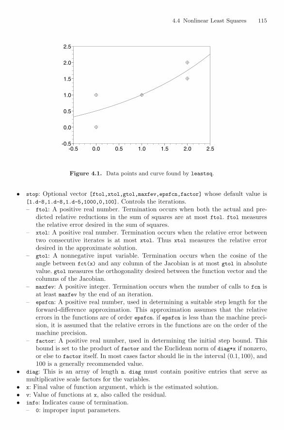
4.4 Nonlinear Least Squares 115
-0.5 0.0 0.5 1.0 1.5 2.0 2.5-0.5
0.0
0.5
1.0
1.5
2.0
2.5
Figure 4.1. Data points and curve found by leastsq.
• stop: Optional vector [ftol,xtol,gtol,maxfev,epsfcn,factor] whose default value is[1.d-8,1.d-8,1.d-5,1000,0,100]. Controls the iterations.– ftol: A positive real number. Termination occurs when both the actual and pre-
dicted relative reductions in the sum of squares are at most ftol. ftol measuresthe relative error desired in the sum of squares.
– xtol: A positive real number. Termination occurs when the relative error betweentwo consecutive iterates is at most xtol. Thus xtol measures the relative errordesired in the approximate solution.
– gtol: A nonnegative input variable. Termination occurs when the cosine of theangle between fct(x) and any column of the Jacobian is at most gtol in absolutevalue. gtol measures the orthogonality desired between the function vector and thecolumns of the Jacobian.
– maxfev: A positive integer. Termination occurs when the number of calls to fcn isat least maxfev by the end of an iteration.
– epsfcn: A positive real number, used in determining a suitable step length for theforward-difference approximation. This approximation assumes that the relativeerrors in the functions are of order epsfcn. if epsfcn is less than the machine preci-sion, it is assumed that the relative errors in the functions are on the order of themachine precision.
– factor: A positive real number, used in determining the initial step bound. Thisbound is set to the product of factor and the Euclidean norm of diag*x if nonzero,or else to factor itself. In most cases factor should lie in the interval (0.1, 100), and100 is a generally recommended value.
• diag: This is an array of length n. diag must contain positive entries that serve asmultiplicative scale factors for the variables.
• x: Final value of function argument, which is the estimated solution.• v: Value of functions at x, also called the residual.• info: Indicates cause of termination.
– 0: improper input parameters.
116 4 Optimization
– 1: algorithm estimates that the relative error between x and the solution is at mosttol.
– 2: maximum number of calls to fcn has been reached.– 3: tol is too small. No further improvement in the approximate solution x is possible.– 4: iteration is not making good progress.
The functions describing the equations fct and their Jacobian fjac are of the sameform. Letting fn stand for either fct or fjac, the allowable formats are
• A Scilab function whose calling sequence is v=fn(x,m) given x and m.• A character string that refers to a C or Fortran routine that must be linked to Scilab.
Should return −1 in iflag to stop the algorithm if the function or Jacobian could notbe evaluated– Fortran calling sequence should be fct(m,n,x,v,iflag), where m, n, iflag are inte-
gers, x is a double-precision vector of size n and v a double-precision vector of sizem.
– C calling sequence should befct(int *m, int *n, double x[],double v[],int *iflag)
Suppose that we wish not to use leastsq on our previous example, but wish to uselsqrsolve. The format of the function is slightly different due to the parameter m, but wecan reuse our previous function by using the following script.
DAT=[0 0;0 1;1 1;2 1.5; 2 2];
function z=fun(p)
DAT=[0 0;0 1;1 1;2 1.5; 2 2]
z=DAT(:,2)-p(1)*exp(p(2)*DAT(:,1))-p(3)
endfunction
p0=[0 0 0];
function z=fct(p,m)
z=fun(p)
endfunction
[p,v]=lsqrsolve(p0,fct,5);
xbasc();
plot2d(DAT(:,1),DAT(:,2),-3,rect=[-0.5,-0.5,2.5,2.5]) ← Fig. 4.2t=linspace(-0.5,2.5,50);
et=p(1)*exp(p(2)*t)+p(3);
plot2d(t,et,rect=[-0.5,-0.5,2.5,2.5])
Note that we are using the same equations and the same initial guess as before. Thevalue of p is completely different from the one we found before.
�−→ p
p =
! - 4154.231 - 0.0001505 4154.706 !
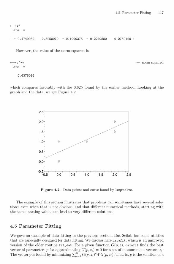
4.5 Parameter Fitting 117
�−→ v’
ans =
! - 0.4749930 0.5250070 - 0.1000375 - 0.2249880 0.2750120 !
However, the value of the norm squared is
�−→ v’*v ← norm squaredans =
0.6375094
which compares favorably with the 0.625 found by the earlier method. Looking at thegraph and the data, we get Figure 4.2.
-0.5 0.0 0.5 1.0 1.5 2.0 2.5-0.5
0.0
0.5
1.0
1.5
2.0
2.5
Figure 4.2. Data points and curve found by lsqrsolve.
The example of this section illustrates that problems can sometimes have several solu-tions, even when that is not obvious, and that different numerical methods, starting withthe same starting value, can lead to very different solutions.
4.5 Parameter Fitting
We gave an example of data fitting in the previous section. But Scilab has some utilitiesthat are especially designed for data fitting. We discuss here datafit, which is an improvedversion of the older routine fit_dat. For a given function G(p, z), datafit finds the bestvector of parameters p for approximating G(p, zi) = 0 for a set of measurement vectors zi.The vector p is found by minimizing
∑ni=1 G(p, zi)′WG(p, zi). That is, p is the solution of a
118 4 Optimization
weighted least squares problem. The most common use of W is to make some measurementsmore important than others. This utility uses optim, so the full calling sequence has manyof the same optional variables.
The simplest call to datafit requires only the form of the equation G, the data, and astarting guess for the parameters p. In this case the calling sequence takes the form
�−→ [p,err]=datafit(G,Z,p0)
Let ne, np, nz be the number of equations in G, the number of parameters in p, and thesize of a single observation (dimension of z) respectively. Then
• G is a function describing e=G(p,z).• Z is the matrix of observations [z_1,z_2,...,z_n], where each measurement is a column
vector.• p0 is the initial guess for the parameters.
For example, if we wished to fit the data of the example in the last section, we coulduse the following Scilab script:
�−→ Z=[0 0 1 2 2;0 1 1 1.5 2];
�−→ function e=G(p,z)
�−→ e=z(2)-p(1)*exp(p(2)*z(1))-p(3)
�−→ endfunction
�−→ p0=[0 0 0]’;
Note that the initial p0 had to be put in as a column vector. When this script isexecuted we get the output
�−→ [p,err]=datafit(G,Z,p0);
which is the same as that given by leastsq in the last section.We saw in the last section that there can be more than one solution to a parameter-
fitting problem. It can be important to bound the parameters to avoid values that arenot physically correct. Also, sometimes some data are more important than other data.In this case one wants to weight the data. Sometimes the default values of parameters donot enable the algorithm to converge. These and other considerations sometimes requireaccess to more of the parameters inside the algorithm. The full calling sequence, whichshares a number of variables with optim, is
[p,err]=datafit([imp,] G [,DG],Z [,W],[contr],p0,[algo],[df0,[mem]],
[work],[stop],[’in’])
These parameters are as follows:
• imp: Scalar argument used to set the trace mode. imp=0 means that nothing (excepterrors) is reported. imp=1 means initial and final reports, imp=2 adds a report periteration and imp>2 adds reports on linear search. Note that most of these reports arewritten on the Scilab standard output.
• DG: Partial of G with respect to p. In the form S=DG(p,z), so that S is ne×np.• W: Weighting matrix of size ne×ne. Default is the identity.
4.6 Linear and Quadratic Programming 119
• "in": Reserved keyword for initialization of parameters used when G is given as aFortran or C routine.
• p: Optimal solution found, given as a column vector.• err: Least squares error.
All the remaining parameters are identical to those in the general call to optim.
4.6 Linear and Quadratic Programming
4.6.1 Linear Programs
The basic linear programing problem is to minimize p′x subject to linear constraints. Theselinear constraints can be equality or inequality constraints. The inequality constraints canbe one-sided or bound constraints. The Scilab function to solve these problems is linpro.The general form of the problem is
minx p′x, (4.12a)C1x ≤ b1, (4.12b)
ci ≤ x ≤ cs, (4.12c)C2x = b2. (4.12d)
The form of the calling sequence depends on how many of these types of constraints arepresent. The calling sequences are
[x,lagr,f]=linpro(p,C,b [,x0])
[x,lagr,f]=linpro(p,C,b,ci,cs [,x0])
[x,lagr,f]=linpro(p,C,b,ci,cs,me [,x0])
[x,lagr,f]=linpro(p,C,b,ci,cs,me,x0 [,imp])
The first three of these correspond to having the constraints (4.12b), (4.12b) and (4.12c),(4.12b)–(4.12d) respectively. Note that if there are no constraints at all, then the problemhas no finite solution if p is not the zero vector.
These parameters have the following meaning:
• p: Real column vector of dimension n that contains the coefficients of the linear costfunction.
• C: Real (me + md)×n matrix. If no constraints are given, that is, all constraints areof the form (4.12c), you can set C = []. Equality constraints are listed first, so thatif both (4.12b) and (4.12d) are present, we have C(j,:)x = b(j) for j=1,...,me andC(j,:)x <= b(j), for j=me+1,...,me+md.
• b: (me + md)-dimensional column vector that is the right hand of the constraints in(4.12b), (4.12d). If no constraints are given, then you can set b = [].
• ci: n-dimensional column vector of lower bounds. If there are no lower bound con-straints, put ci = []. If some components of x are bounded from below, set the other(unconstrained) values of ci to a negative number that has very large magnitude. Thatis, ci(j)=-number_properties(’huge’).
• cs: Column vector of upper bounds. See comments for ci.• me: Number of equality constraints. Thus C(1:me,:)*x = b(1:me).• x0: Either an initial guess for x or one of the character strings ’v’ or ’g’. If x0=’v’,
then the calculated initial feasible point is a vertex. If x0=’g’, then the calculated initialfeasible point need not be a vertex.
120 4 Optimization
• imp: This is the verbose option. (Try imp= 7, 8 . . .). Note that the messages are sent toScilab standard output (can be lengthy if there are many iterations).
• x: Optimal solution found by algorithm.• f: Optimal value of the cost function (4.12a).• lagr: This is a vector of Lagrange multipliers. If lower and upper-bounds ci,cs are
provided, lagr has n+me+md components and lagr(1:n) is the Lagrange vector associatedwith the bound constraints and lagr(n+1: n+me+md) is the Lagrange vector associatedwith the linear constraints. If an upper bound (respectively lower bound) constraint i
is active, then lagr(i) is greater than 0 (resp. <0). If no bounds are provided, thenlagr has only me+md components.
4.6.2 Quadratic Programs
A quadratic program is the same as (4.12) except that the cost function (4.12a) is replacedby the quadratic expression
12x′Qx + p′x. (4.13)
The utility provided by Scilab is quapro. Since quapro does not require Q to be positivedefinite, in fact Q could be zero, quapro can solve linear programming problems. With theexception of the matrix Q, which must be real symmetric, the calling sequence for quapro
is identical to that of linpro. Since the variables have the same meanings, we do no repeattheir definitions here. The possible calling sequence for quapro are
[x,lagr,f]=quapro(Q,p,C,b [,x0])
[x,lagr,f]=quapro(Q,p,C,b,ci,cs [,x0])
[x,lagr,f]=quapro(Q,p,C,b,ci,cs,me [,x0])
[x,lagr,f]=quapro(Q,p,C,b,ci,cs,me,x0 [,imp])
4.6.3 Semidefinite Programs
There is also a Scilab function for solving semidefinite programs called semidef:
[x,Z,ul,info]=semidef(x0,Z0,F,blck_szs,c,options)
However, we shall not discuss it here. The interested reader is referred to the on-line help.
4.7 Differentiation Utilities
The function NDcost was introduced earlier to enable the user to solve some problemswithout having to specify the gradient. Other utilities described earlier will automaticallyestimate derivatives or Jacobians numerically when this is requested. However, it is some-times useful to be able to get numerical estimates of derivatives and Jacobians directly.This capability is provided by numdiff and derivative.
The Scilab function numdiff computes a numerical estimate of the Jacobian using finitedifference methods. If the function has real-number values, then it gives an estimate of thegradient. Its calling sequence is
g=numdiff(fun,x [,dx])
if there are no parameters in fun. The parameters in numdiff are
4.7 Differentiation Utilities 121
• fun: An external describing the function to be differentiated. The function fun calling se-quence must be y=fun(x,p1,p2,...,pn), where the pi are optional parameters. If param-eters p1,p2,...,pn exist, then numdiff can be called by g=numdiff(list(fun,p1,p2,...,pn),x).
• x: Vector argument of the function fun.• dx: Vector, which is the finite difference step. Default value is
dx=sqrt(%eps)*(1+1d-3*abs(x))
• g: Vector (matrix), which is the estimated gradient (Jacobian).
For example, suppose that we want the Jacobian (derivative) of
f(x1, x2, x3) =(
x1 + 2x22x3
sin(x1x2x3)
)at x =
⎛⎝1
23
⎞⎠ . (4.14)
The following Scilab script, when executed, computes the estimate of the Jacobian givenby numdiff, the true Jacobian, and their difference.
function z=myf(x)
z=[x(1)+2*x(2)-x(2)^2*x(3);sin(x(1)*x(2)*x(3))]
endfunction
x=[1;2;3];
J=numdiff(myf,x);
TrueJ=[1,2-2*x(2)*x(3), -x(2)^2];
a=cos(x(1)*x(2)*x(3));
TrueJ=[TrueJ;a*[x(3)*x(2),x(1)*x(3),x(1)*x(2)]];
Difference=J-TrueJ;
The solution is
�−→ J
J =
! 1.0000000 - 10. - 4. !
! 5.7610218 2.8805109 1.9203406 !
�−→ TrueJ
TrueJ =
! 1. - 10. - 4. !
! 5.7610217 2.8805109 1.9203406 !
�−→ Difference
Difference =
! - 1.286D-08 - 4.045D-08 3.518D-08 !
! 1.157D-07 5.690D-08 - 1.100D-08 !
122 4 Optimization
4.7.1 Higher Derivatives
Sometimes it is desirable to have higher derivatives. Numerical differentiation is prone toill conditioning and error and this is especially true with the higher derivatives. If high-accuracy higher derivatives are required, the best alternatives are symbolic differentiationusing a symbolic language such as Maple or automatic differentiation using a package suchas ADOL-C. [24] For complicated problems the symbolic approach can be very slow andhave memory problems. The only choice then may be automatic differentiation.
If the needed derivatives are limited to first and second order, then useful approximatederivatives can often by gotten by using the Scilab function derivative.
Suppose that we have a function such as (4.15) of an n-dimensional vector x withvalues that are m-dimensional vectors. Then at a point a it has a Taylor expansion
f(x) =
⎛⎜⎝
f1(x)...
fm(x)
⎞⎟⎠ = f(a) + J(a)(x − a) +
⎛⎜⎝
(x − a)′H1(a)(x − a)...
(x − a)′Hm(a)(x − a)
⎞⎟⎠ + · · · . (4.15)
Thus the first derivative is just the m × n Jacobian matrix J . However, the secondderivative is now m matrices each of which is n × n. The first and second derivatives off are provided by derivative. This utility provides several choices on how to arrange theinformation on the second derivative by use of the H_form variable. The full calling syntaxis
[J [,H]] = derivative(F,x [,h ,order ,H_form ,Q])
• F: Scilab function F or a list(F,p1,...,pk), where F is a Scilab function in the formy=F(x,p1,...,pk), with p1, ..., pk being any Scilab objects such as matrices or lists.
• x: real column vector of dimension n.• h: Step size used in the finite difference approximations. Usually better to leave to
software to choose.• order: Integer that is the order of the finite difference formula used to approximate the
derivatives. Default is order= 2. May be chosen as 1, 2, or 4.• H_form: String giving the form in which the Hessian will be returned.
– H_form=’default’: H is an m×(n^2) matrix. Here the kth row of H corresponds to theHessian of the kth component of F.
– H_form=’blockmat’: In this format H is a (m×n)×n block matrix . Thus, in Scilabnotation, H = [H1;H2; ... ;Hm].
– H_form=’hypermat’: H is a n×n matrix for m=1, and a n×n×m hypermatrix otherwise.That is, H(:,:,k) is the classical Hessian matrix of the kth component of F.
• Q: Real orthogonal matrix. Default is eye(n,n).
The Jacobian is computed by approximating the directional derivatives of the compo-nents of F in the direction of the columns of Q. The second derivatives are computed bycomposition of first-order derivatives. Numerical approximation of derivatives is generallyan unstable process. The step size h must be small to get a low error, but if it is too small,floating-point errors will dominate by cancellation. A rule of thumb is not to change thedefault step size. To work around numerical difficulties one may also change the orderand/or choose different orthogonal matrices Q (the default is eye(n,n)), especially if theapproximate derivatives are used in optimization routines. All the optional arguments mayalso be passed as named arguments.
As an illustration suppose that myf is the same function as in the previous exampleand that it and x are already in the workspace. Then the second derivative will have two3 × 3 matrices. If we choose ’hypermat’ for the output format, then we will obtain
4.7 Differentiation Utilities 123
�−→ function z=myf(x)
�−→ z=[x(1)+2*x(2)-x(2)^2*x(3);sin(x(1)*x(2)*x(3))]
�−→ endfunction�−→ x=[1;2;3];
�−→ [J,H]=derivative(myf,x,H_form=’hypermat’)
H =
(:,:,1)
! 0. 0. 0. !
! 0. - 6. - 4. !
! 0. - 4. 0. !
(:,:,2)
! 10.058956 7.9099883 5.2733256 !
! 7.9099883 2.5147394 2.6366631 !
! 5.2733256 2.6366631 1.117662 !
J =
! 1. - 10. - 4. !
! 5.7610217 2.8805109 1.9203406 !
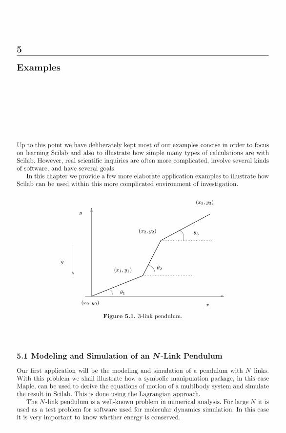
5
Examples
Up to this point we have deliberately kept most of our examples concise in order to focuson learning Scilab and also to illustrate how simple many types of calculations are withScilab. However, real scientific inquiries are often more complicated, involve several kindsof software, and have several goals.
In this chapter we provide a few more elaborate application examples to illustrate howScilab can be used within this more complicated environment of investigation.
x
θ2
θ3
(x3, y3)
(x2, y2)
(x1, y1)
θ1
g
y
(x0, y0)
Figure 5.1. 3-link pendulum.
5.1 Modeling and Simulation of an N -Link Pendulum
Our first application will be the modeling and simulation of a pendulum with N links.With this problem we shall illustrate how a symbolic manipulation package, in this caseMaple, can be used to derive the equations of motion of a multibody system and simulatethe result in Scilab. This is done using the Lagrangian approach.
The N -link pendulum is a well-known problem in numerical analysis. For large N it isused as a test problem for software used for molecular dynamics simulation. In this caseit is very important to know whether energy is conserved.
126 5 Examples
The N -link pendulum also arises as a model for flexible cables and chains. Several yearsago there was a collapse of several towers carrying power. It turned out that the powerlines were supported by pairs of chains of insulators and one of these chains had failed andthe other was unable to continue to support the power line. In the followup studies, theinsulator chains were modeled as 16-link pendulums.
5.1.1 Equations of Motion of the N-Link Pendulum
In this application we wish to simulate the motion of an N -link pendulum fixed at oneextremity and moving without friction in a vertical plane. As an example, and for fixingnotation, a picture of a 3-link pendulum is given in Figure 5.1. The equation of motioncan easily be deduced from a Lagrangian formulation for a 1- or 2-link pendulum but itcan become tedious work for say a 10-link pendulum in the Scilab demos.
In order to construct models with large N , we use the computer algebra packageMaplein order to derive the equations of motion from a Lagrangian formulation. Thecomputer algebra package generates Fortran code to be used by Scilab for simulation. Italso provides LATEX code for symbolic expressions at every step of the computation. TheN -link pendulum is considered as N independant connected rigid bodies.
The Maple code is separated into two parts. The first part provides a general libraryfor Lagrangian modeling of rigid bodies linked with holonomic constraints, and the secondpart applies the general code to the specific example of the N -link pendulum. By settingthe code up in this manner, we have made it easier for the reader to modify the pendu-lum problem, say by adding masses at the end or even modeling a completely differentmechanical system.
It should be noted that the kind of constraints we have here are called holonomic.Constraints involving velocities are called nonholonomic and are not considered here.
Lagrangian of Multibody Systems with Holonomic Constraints
Let q be the generalized coordinates and q the generalized velocities of the system of Nrigid bodies. The coordinates q can vary with time t. Then the Lagrangian of the problemcan be expressed as
L(q, q) =N∑
i=1
Li(q, q), (5.1)
where Li is the Lagrangian of body i. For each component of q we have to computeI(q, q, q)i, which is defined by the Euler equation
I(q, q, q)i =d
dt
(∂L∂qi
)− ∂L
∂qi.
Readers familiar with the calculus of variations or optimal control will recognize this asthe usual term that arises in the necessary conditions for a minimum.
This formal expression for I(q) can be rewritten in matrix notation as
I(q, q, q) = M(q)q + R(q, q). (5.2)
If there are no constraints or outside forces, then (5.2) is set equal to zero, and we get theusual second-order equation of motion, which says that mass times acceleration is equalto the total force.

5.1 Modeling and Simulation of an N -Link Pendulum 127
So far we have assumed that the rigid bodies were independent. We now have to dealwith the mechanical constraints of holonomic type expressing the fact that we have a linkedpendulum. These constraints can be written as A(q) = 0. Note that the time derivative ofthe constraints gives the equation
B(q)q = 0,
where B(q) = dBdq , that is,
B(q)i,j =(
∂A(q)i
∂qj
).
Thus q has to be in the kernel of B(q). We can then try to compute a formal basis of thekernel of B(q). This yields a matrix S(q) whose columns span the kernel of B(q). Then wecan introduce a time function η such that q = S(q)η. Note that by definition we have
B(q)S(q)η = 0. (5.3)
We return now to the Euler equations. Using the constraints and their associatedLagrange multipliers, the equations can be expressed as
I(q, q, q) = B(q)T λ. (5.4)
We use S(q) to eliminate the right-hand side of (5.4) by left multiplying by S(q)T andsimplifying the result using q = S(q)η and its time derivative, which can be expressed asq = W (q, η, η). We finally obtain
0 = S(q)TI(q, q, q) = M1(q)η + R1(q, η).
The dynamical system with state (q, η) to be simulated is then
M1(q)η + R1(q, η) = 0, (5.5a)q − S(q)η = 0. (5.5b)
Note that in this last equation the constraint A(q) = 0 is seen only through its timederivative. This raises the possibility that during simulation there may be numerical er-rors in the constraints. In the numerical analysis literature this is called constraint drift.However, we will see that in the example of the N -link pendulum, we can simplify theequations in order to avoid the numerical drift in the constraint A(q) = 0.
When it is not possible to find a formal basis of the null space of B(q), it is oftenpossible to differentiate the holonomic constraint twice, which leads to the constraint
B(q)q + Bq(q)q = 0.
Thus we have A(q) = 0, B(q)q = 0, and B(q)q + Bq(q)q = 0. These three constraints canbe replaced by a unique constraint [9]
−B(q)q + R2(q, q) = 0
withR2(q, q) = −Bq(q)q + α (B(q)q) + βA(q) = 0.
This replacement process is known as stabilized differentiation or Baumgarte stabilization.The new system to be simulated is then
M(q)q − B(q)T λ + R(q, q) = 0, (5.6a)−B(q)q + R2(q, q) = 0. (5.6b)
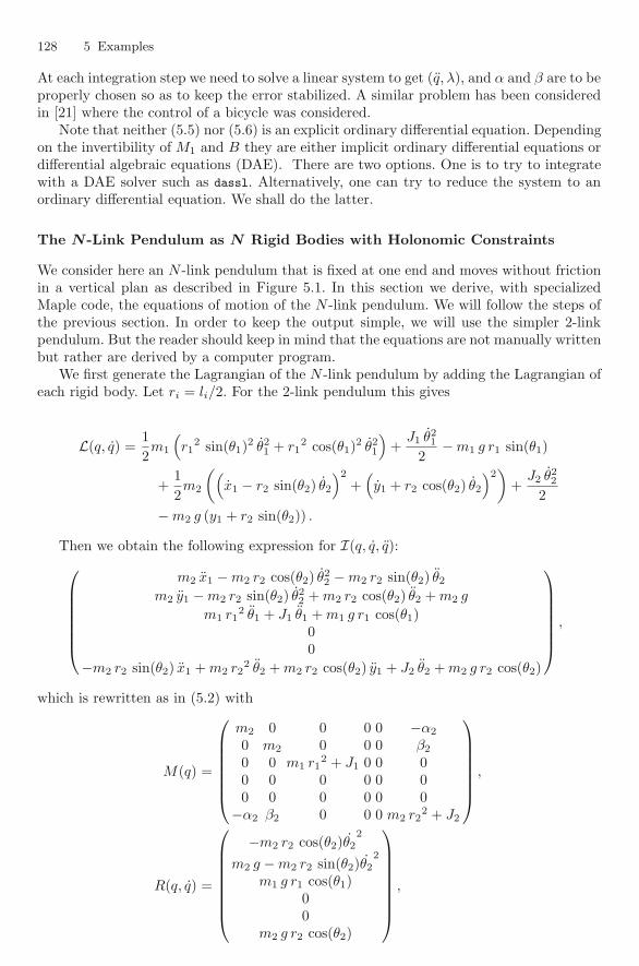
128 5 Examples
At each integration step we need to solve a linear system to get (q, λ), and α and β are to beproperly chosen so as to keep the error stabilized. A similar problem has been consideredin [21] where the control of a bicycle was considered.
Note that neither (5.5) nor (5.6) is an explicit ordinary differential equation. Dependingon the invertibility of M1 and B they are either implicit ordinary differential equations ordifferential algebraic equations (DAE). There are two options. One is to try to integratewith a DAE solver such as dassl. Alternatively, one can try to reduce the system to anordinary differential equation. We shall do the latter.
The N-Link Pendulum as N Rigid Bodies with Holonomic Constraints
We consider here an N -link pendulum that is fixed at one end and moves without frictionin a vertical plan as described in Figure 5.1. In this section we derive, with specializedMaple code, the equations of motion of the N -link pendulum. We will follow the steps ofthe previous section. In order to keep the output simple, we will use the simpler 2-linkpendulum. But the reader should keep in mind that the equations are not manually writtenbut rather are derived by a computer program.
We first generate the Lagrangian of the N -link pendulum by adding the Lagrangian ofeach rigid body. Let ri = li/2. For the 2-link pendulum this gives
L(q, q) =12m1
(r1
2 sin(θ1)2 θ21 + r1
2 cos(θ1)2 θ21
)+
J1 θ21
2− m1 g r1 sin(θ1)
+12m2
((x1 − r2 sin(θ2) θ2
)2
+(y1 + r2 cos(θ2) θ2
)2)
+J2 θ2
2
2− m2 g (y1 + r2 sin(θ2)) .
Then we obtain the following expression for I(q, q, q):⎛⎜⎜⎜⎜⎜⎜⎝
m2 x1 − m2 r2 cos(θ2) θ22 − m2 r2 sin(θ2) θ2
m2 y1 − m2 r2 sin(θ2) θ22 + m2 r2 cos(θ2) θ2 + m2 g
m1 r12 θ1 + J1 θ1 + m1 g r1 cos(θ1)
00
−m2 r2 sin(θ2) x1 + m2 r22 θ2 + m2 r2 cos(θ2) y1 + J2 θ2 + m2 g r2 cos(θ2)
⎞⎟⎟⎟⎟⎟⎟⎠
,
which is rewritten as in (5.2) with
M(q) =
⎛⎜⎜⎜⎜⎜⎜⎝
m2 0 0 0 0 −α2
0 m2 0 0 0 β2
0 0 m1 r12 + J1 0 0 0
0 0 0 0 0 00 0 0 0 0 0
−α2 β2 0 0 0 m2 r22 + J2
⎞⎟⎟⎟⎟⎟⎟⎠
,
R(q, q) =
⎛⎜⎜⎜⎜⎜⎜⎜⎝
−m2 r2 cos(θ2)θ22
m2 g − m2 r2 sin(θ2)θ22
m1 g r1 cos(θ1)00
m2 g r2 cos(θ2)
⎞⎟⎟⎟⎟⎟⎟⎟⎠
,
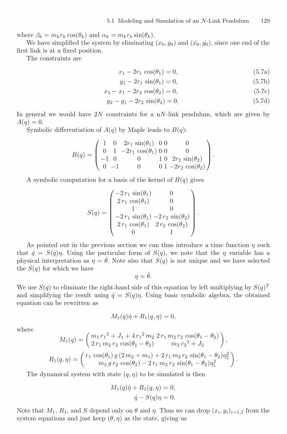
5.1 Modeling and Simulation of an N -Link Pendulum 129
where βk = mkrk cos(θk) and αk = mkrk sin(θk).We have simplified the system by eliminating (x0, y0) and (x0, y0), since one end of the
first link is at a fixed position.The constraints are
x1 − 2r1 cos(θ1) = 0, (5.7a)y1 − 2r1 sin(θ1) = 0, (5.7b)
x2 − x1 − 2r2 cos(θ2) = 0, (5.7c)y2 − y1 − 2r2 sin(θ2) = 0. (5.7d)
In general we would have 2N constraints for a nN -link pendulum, which are given byA(q) = 0.
Symbolic differentiation of A(q) by Maple leads to B(q):
B(q) =
⎛⎜⎜⎝
1 0 2r1 sin(θ1) 0 0 00 1 −2r1 cos(θ1) 0 0 0−1 0 0 1 0 2r2 sin(θ2)0 −1 0 0 1 −2r2 cos(θ2)
⎞⎟⎟⎠ .
A symbolic computation for a basis of the kernel of B(q) gives
S(q) =
⎛⎜⎜⎜⎜⎜⎜⎝
−2 r1 sin(θ1) 02 r1 cos(θ1) 0
1 0−2 r1 sin(θ1) −2 r2 sin(θ2)2 r1 cos(θ1) 2 r2 cos(θ2)
0 1
⎞⎟⎟⎟⎟⎟⎟⎠
.
As pointed out in the previous section we can thus introduce a time function η suchthat q = S(q)η. Using the particular form of S(q), we note that the η variable has aphysical interpretation as η = θ. Note also that S(q) is not unique and we have selectedthe S(q) for which we have
η = θ.
We use S(q) to eliminate the right-hand side of this equation by left multiplying by S(q)T
and simplifying the result using q = S(q)η. Using basic symbolic algebra, the obtainedequation can be rewritten as
M1(q)η + R1(q, η) = 0,
where
M1(q) =(
m1 r12 + J1 + 4 r1
2 m2 2 r1 m2 r2 cos(θ1 − θ2)2 r1 m2 r2 cos(θ1 − θ2) m2 r2
2 + J2
),
R1(q, η) =(
r1 cos(θ1) g (2m2 + m1) + 2 r1 m2 r2 sin(θ1 − θ2)η22
m2 g r2 cos(θ2) − 2 r1 m2 r2 sin(θ1 − θ2)η21
).
The dynamical system with state (q, η) to be simulated is then
M1(q)η + R1(q, η) = 0,q − S(q)η = 0.
Note that M1, R1, and S depend only on θ and η. Thus we can drop (xi, yi)i=1,2 from thesystem equations and just keep (θ, η) as the state, giving us
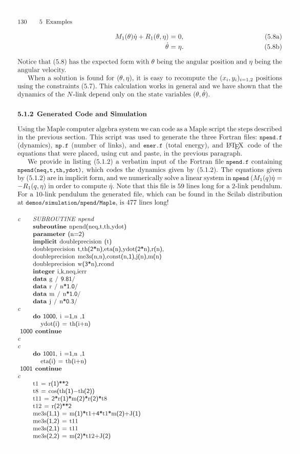
130 5 Examples
M1(θ)η + R1(θ, η) = 0, (5.8a)θ = η. (5.8b)
Notice that (5.8) has the expected form with θ being the angular position and η being theangular velocity.
When a solution is found for (θ, η), it is easy to recompute the (xi, yi)i=1,2 positionsusing the constraints (5.7). This calculation works in general and we have shown that thedynamics of the N -link depend only on the state variables (θ, θ).
5.1.2 Generated Code and Simulation
Using the Maple computer algebra system we can code as a Maple script the steps describedin the previous section. This script was used to generate the three Fortran files: npend.f(dynamics), np.f (number of links), and ener.f (total energy), and LATEX code of theequations that were placed, using cut and paste, in the previous paragraph.
We provide in listing (5.1.2) a verbatim input of the Fortran file npend.f containingnpend(neq,t,th,ydot), which codes the dynamics given by (5.1.2). The equations givenby (5.1.2) are in implicit form, and we numerically solve a linear system in npend (M1(q)η =−R1(q, η) in order to compute η. Note that this file is 59 lines long for a 2-link pendulum.For a 10-link pendulum the generated file, which can be found in the Scilab distributionat demos/simulation/npend/Maple, is 477 lines long!
c SUBROUTINE npendsubroutine npend(neq,t,th,ydot)parameter (n=2)implicit doubleprecision (t)doubleprecision t,th(2*n),eta(n),ydot(2*n),r(n),doubleprecision me3s(n,n),const(n,1),j(n),m(n)doubleprecision w(3*n),rcondinteger i,k,neq,ierrdata g / 9.81/data r / n*1.0/data m / n*1.0/data j / n*0.3/
cdo 1000, i =1,n ,1
ydot(i) = th(i+n)1000 continue
cc
do 1001, i =1,n ,1eta(i) = th(i+n)
1001 continuec
t1 = r(1)**2t8 = cos(th(1)−th(2))t11 = 2*r(1)*m(2)*r(2)*t8t12 = r(2)**2me3s(1,1) = m(1)*t1+4*t1*m(2)+J(1)me3s(1,2) = t11me3s(2,1) = t11me3s(2,2) = m(2)*t12+J(2)

5.1 Modeling and Simulation of an N -Link Pendulum 131
t1 = m(2)*r(2)t2 = eta(2)**2t4 = sin(th(1)−th(2))t8 = cos(th(1))t16 = eta(1)**2t20 = cos(th(2))const(1,1) = r(1)*(2*t1*t2*t4+2*t8*m(2)*g+m(1)*g*t8)const(2,1) = t1*(−2*r(1)*t16*t4+g*t20)
cdo 1002, i =1,n ,1
const(i,1) = −const(i,1)1002 continue
cc solving M z = const to obtain ydot((n+1). .2*n)
call dlslv(me3s,n,n,const,n,1,w, rcond,ierr,1)if (ierr.ne.0) then
write(6,2000)2000 format(’Matrix is badly conditioned’)
endifc
do 1003, i =1,n ,1ydot(n+i) = const(i,1)
1003 continuec
returnend
As described in Section 2.5.1 on interfacing, it is now possible to link the functionnpend (which conforms to the internal calling syntax accepted by ode), and numericallyintegrate the N -pendulum equation using ode. The np function, which is also dynamicallylinked in Scilab, returns the number of links of the pendulum. The reader can take a lookat the SCI/demos/simulation/npend to check the details. The Fortran code is compiledand dynamically linked in a running Scilab using the previously described ilib_for_link
function.
�−→ npend_build_and_load() ; ← calling ilib_for_link
generate a loader file
generate a Makefile: Makelib
running the makefile
compilation of npend
compilation of np
compilation of ener
compilation of dlslv
building shared library (be patient)
shared archive loaded
Link done
�−→ n=np(); r=ones(1,n); m=ones(1,n); j=ones(1,n); g=9.81;
�−→ y0=0*ones(2*n,1);tt=0:0.05:10; ← (θ, θ)(0) = 0�−→ yt=ode(y0,0,tt,’npend’); ← calling ode
�−→ draw_chain_from_angles(yt(1:$/2,:),r,1); ← Figure˜5.2

132 5 Examples
Then the N -link pendulum is easily simulated using ode given initial values for (θ, θ).Using the scilab demo files, we now show the result (See Figure 5.2) of a simulation of a10-link pendulum.
Figure 5.2. 10-link pendulum. Dotted line represents the trajectory of the endpoint of thependulum.
The result of the ode simulation is a matrix with N rows. Each column of thematrix gives the value of (θ, θ) at a specific time. Using this matrix a graphics sim-ulation is obtained by first computing the (xi, yi)i=0,N and then using the functiondraw_chain_from_angles to provide an animation. There is an option in the animationto keep track of the trajectory of the endpoint of the pendulum. This curve can be seenas the dashed line in the static Figure 5.2.
We provide here a slightly modified version of draw_chain_from_angles, which gives anexample of an animation using the new graphics mode. Moreover, this function uses theScilab functions realtimeinit and realtime to control the animation speed.
function draw_chain_from_angles(a,r,job,rt)
// a the angles , a(i,j) is the angle of node i at time t(j)
// r the segments half length
if argn(2)<3 then job=0, endif argn(2)<4 then rt = 0.01; endn2=size(a,2);
x=[0*ones(1,n2);cumsum(2*diag(r)*cos(a),1)];
y=[0*ones(1,n2);cumsum(2*diag(r)*sin(a),1)];
draw_chain_from_coordinates(x,y,job,rt)
endfunction
function draw_chain_from_coordinates(x,y,job,rt)
// x(i,j), y(i,j) is the coordinate of node i at time t(j)
5.1 Modeling and Simulation of an N -Link Pendulum 133
// r the segments half length
if argn(2)<3 then job=0, endif argn(2)<4 then rt = 0.01; end[n1,n2]=size(x);
b = maxi(maxi(abs(x)),maxi(abs(y)));
xbasc();set figure_style new; ← new graphics modea=gca() ← we want to seta.data_bounds=[-1,-1;1,0]*b; ← the graphics boundariesa.isoview="on"; ← and use an isoview modexset(’pixmap’,1); ← double buffer modedrawlater() ← wait for graphics displaycolors= 1:n1-1; colors(8)=n1;
xsegs([x(1:$-1,1)’;x(2:$,1)’],[y(1:$-1,1)’;y(2:$,1)’],colors) ← drawp=gce();p.thickness=4; ← p is used to keep track of xsegs dataif job==1 then
xpoly(x($,1)*ones(2,1),y($,1)*ones(2,1),’lines’); ← endpoint trajectoryt=gce();t.line_style=2;
enddrawnow() ← perform drawingxset(’wshow’) ← update display with double bufferind=[1;(2:n1-1)’.*.ones(2,1);n1]
realtimeinit(rt); ← set time unit: smaller values will accelerate the animationfor j=1:n2,
realtime(j) ← wait to time j before continuingdrawlater()
p.data = [x(ind,j),y(ind,j)]; ← update xsegs dataif job==1 then t.data=[t.data;[x($,j),y($,j)]], end ← update xpoly datadrawnow() ← since objects are updated, graphics is cleared and redrawnxset(’wshow’) ← update display with double buffer
endendfunction
5.1.3 Maple Code
General Code Dealing with Euler Equation
We provide here part of the file Euler.map, which contains generic functions for Eulerequation computation from Lagrangian formulation. For simplicity we have removed fromthe Maple code functions devoted to LATEX code generation, but the full file content canbe found in the Scilab distribution.
#---------------------------------------------------------------
# Functions for computing Euler equations. L is the Lagrangian,
# q,qd,qdd are the generalized coordinates and their derivatives
#---------------------------------------------------------------
with(‘linalg‘):
euler_equations:=proc(L,q,qd,qdd)
local k,m:
m:=nops(q);
v:=matrix(m,1,0);
for i to m do
134 5 Examples
v[i,1]:=LL(q[i])=simplify(time_diff(diff(L,qd[i]),q,qd,qdd)
-diff(L,q[i]));
od;
eval(v):
end:
#---------------------------------------------------------------
# Time derivative computation of an expression
# depending on q,qd,qdd. Used to compute Euler equations
#---------------------------------------------------------------
ttvar:=proc(xx)
if type(xx,‘indexed‘)
then cat(op(0,xx),‘d‘)[op(xx)]
else cat(xx,‘d‘) fi
end:
time_diff:=proc(phi,q,qd,qdd)
local phi_copy,k,diff_phi:
# substitution to specify that q,qd ,qdd depends on time
phi_copy:=phi:
phi_copy:=subs(map( xx-> xx=xx(t),[op(q),op(qd)]),phi_copy):
diff_phi:=diff(phi_copy,t):
# substitution to come back to our variables
diff_phi:=subs(map(xx->diff(xx(t),t)=ttvar(xx),[op(q),op(qd)]),
diff_phi):
diff_phi:=subs(map(xx->xx(t)=xx,[op(q),op(qd),op(qdd)]),diff_phi):
end:
#-----------------------------------------------------
# Rewriting the Euler equations to have a canonical form
# .. .
# El= ME(q) q + RE(q,q)
# Computation of ME
# CEuler returns a list [ME,RE];
#-----------------------------------------------------
CEuler:=proc(E,q,qd,qdd)
local Me,Ce,Re:
Me:=MME(E,q,qd,qdd):
Re:=RRE(E,Me,q,qd,qdd):
[eval(Me),eval(Re)]:
end:
MME:=proc(E,q,qd,qdd)
local E1:
E1:=eval(E):
genmatrix([seq(E1[i,1],i=1..nops(qdd))],qdd):
end:
#-----------------------------------------------------
# .
# Extract the RE(q,q) matrix El= ME(q) qdd + RE(q,qd)

5.2 Modeling and Simulation of a Car 135
#-----------------------------------------------------
RRE:=proc(E,ME,q,qd,qdd)
local MM:
MM:=matadd( E,multiply(ME,matrix(nops(q),1,qdd)),1,-1);
MM:=map((x)-> simplify(x),eval(MM)):
end:
#-----------------------------------------------------
# FORTRAN GENERATION
#-----------------------------------------------------
Gener:=proc(filename,fortranlist)
global optimized;
init_genfor();
optimized:=true:
writeto(filename):
genfor(flist):
writeto(terminal):
end:
5.2 Modeling and Simulation of a Car
This example is presented to illustrate the use of the zero-crossing option in the odefunction. is also particularly interesting because it is hybrid in nature. This means thatit has different behaviors in different “states.” In this example the different states arecharacterized by whether or not the wheels of the car are on the ground. Since our 2Dmodel has only two wheels, the system has four states, since each wheel can be on or offthe ground.
The term “state” is being used two ways in this section. If we wanted to be more precise,we would say that the state of the system is composed of both discrete and continuousstates. The discrete part takes on four values depending on the contact of the wheels. Foreach value of the discrete state we have continuous state variables that describe the car.In the model that follows there are the same number of continuous state variables for eachvalue of the discrete state variable. That need not be true in general.
We consider a very simple planar mechanical model so that the equations do notbecome very complex. We will make several simplifying assumptions in order to reducethe complexity of the model, yet keep the essence of the application so that the model’sdynamic behavior remains realistic. It would be easy to modify this example to make iteven more realistic.
5.2.1 Basic Model
The simple 2D model of the car that we consider here includes (see Figure 5.3):
• two parallel suspensions which are massless but have internal damping,• massless wheels of size zero rolling on the ground with no loss of energy due to friction,• a mass m with rotational inertia J in the middle of the massless rod connecting the
top of the suspensions. The length of the rod connecting the top of the suspensions isa constant denoted by l.
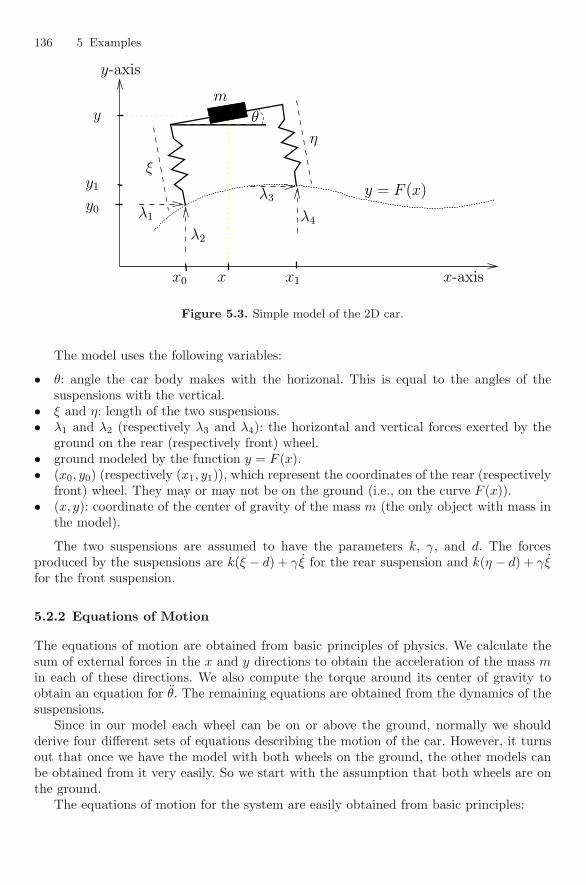
136 5 Examples
η
λ2
x0 x1
y0
y1
y
x
y-axis
λ3
λ4λ1
x-axis
ξ
m
y = F (x)
θ
Figure 5.3. Simple model of the 2D car.
The model uses the following variables:
• θ: angle the car body makes with the horizonal. This is equal to the angles of thesuspensions with the vertical.
• ξ and η: length of the two suspensions.• λ1 and λ2 (respectively λ3 and λ4): the horizontal and vertical forces exerted by the
ground on the rear (respectively front) wheel.• ground modeled by the function y = F (x).• (x0, y0) (respectively (x1, y1)), which represent the coordinates of the rear (respectively
front) wheel. They may or may not be on the ground (i.e., on the curve F (x)).• (x, y): coordinate of the center of gravity of the mass m (the only object with mass in
the model).
The two suspensions are assumed to have the parameters k, γ, and d. The forcesproduced by the suspensions are k(ξ − d) + γξ for the rear suspension and k(η − d) + γξfor the front suspension.
5.2.2 Equations of Motion
The equations of motion are obtained from basic principles of physics. We calculate thesum of external forces in the x and y directions to obtain the acceleration of the mass min each of these directions. We also compute the torque around its center of gravity toobtain an equation for θ. The remaining equations are obtained from the dynamics of thesuspensions.
Since in our model each wheel can be on or above the ground, normally we shouldderive four different sets of equations describing the motion of the car. However, it turnsout that once we have the model with both wheels on the ground, the other models canbe obtained from it very easily. So we start with the assumption that both wheels are onthe ground.
The equations of motion for the system are easily obtained from basic principles:
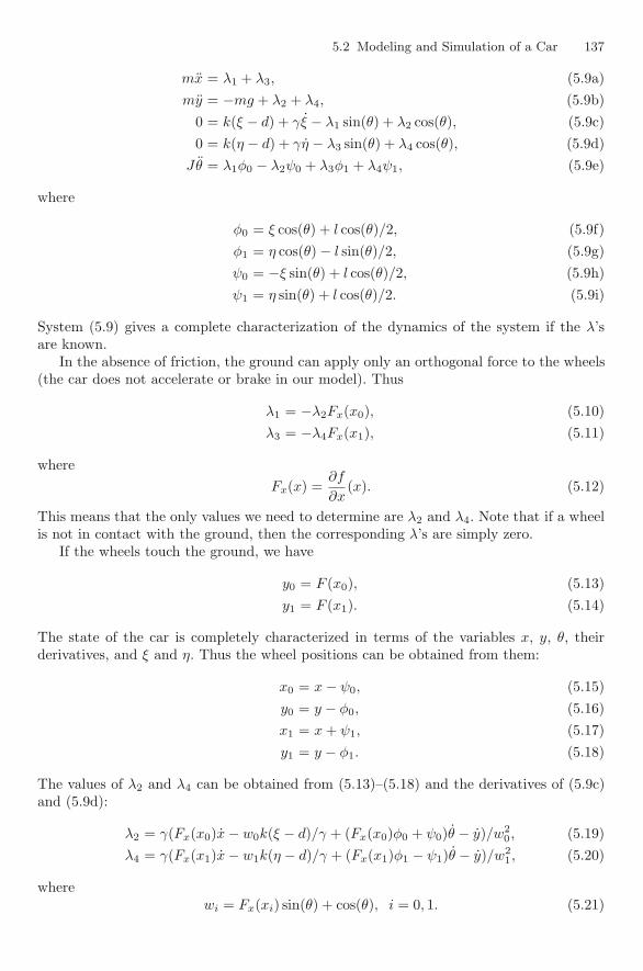
5.2 Modeling and Simulation of a Car 137
mx = λ1 + λ3, (5.9a)my = −mg + λ2 + λ4, (5.9b)
0 = k(ξ − d) + γξ − λ1 sin(θ) + λ2 cos(θ), (5.9c)0 = k(η − d) + γη − λ3 sin(θ) + λ4 cos(θ), (5.9d)
Jθ = λ1φ0 − λ2ψ0 + λ3φ1 + λ4ψ1, (5.9e)
where
φ0 = ξ cos(θ) + l cos(θ)/2, (5.9f)φ1 = η cos(θ) − l sin(θ)/2, (5.9g)ψ0 = −ξ sin(θ) + l cos(θ)/2, (5.9h)ψ1 = η sin(θ) + l cos(θ)/2. (5.9i)
System (5.9) gives a complete characterization of the dynamics of the system if the λ’sare known.
In the absence of friction, the ground can apply only an orthogonal force to the wheels(the car does not accelerate or brake in our model). Thus
λ1 = −λ2Fx(x0), (5.10)λ3 = −λ4Fx(x1), (5.11)
whereFx(x) =
∂f
∂x(x). (5.12)
This means that the only values we need to determine are λ2 and λ4. Note that if a wheelis not in contact with the ground, then the corresponding λ’s are simply zero.
If the wheels touch the ground, we have
y0 = F (x0), (5.13)y1 = F (x1). (5.14)
The state of the car is completely characterized in terms of the variables x, y, θ, theirderivatives, and ξ and η. Thus the wheel positions can be obtained from them:
x0 = x − ψ0, (5.15)y0 = y − φ0, (5.16)x1 = x + ψ1, (5.17)y1 = y − φ1. (5.18)
The values of λ2 and λ4 can be obtained from (5.13)–(5.18) and the derivatives of (5.9c)and (5.9d):
λ2 = γ(Fx(x0)x − w0k(ξ − d)/γ + (Fx(x0)φ0 + ψ0)θ − y)/w20, (5.19)
λ4 = γ(Fx(x1)x − w1k(η − d)/γ + (Fx(x1)φ1 − ψ1)θ − y)/w21, (5.20)
wherewi = Fx(xi) sin(θ) + cos(θ), i = 0, 1. (5.21)
138 5 Examples
5.2.3 Simulation Model
To use the Scilab function ode to simulate this system, we need to put the system intoa first order ODE. This is done by introducing variables vx, vy, and ω to represent thederivatives of x, y and θ. The first-order ODE can now be expressed as follows:
x = vx, (5.22)vx = −(λ2Fx(x0) + λ4Fx(x1))/m, (5.23)y = vy, (5.24)
vy = −(mg − λ2 − λ4)/m, (5.25)
ξ = −(k(ξ − d) + λ2w0)/γ, (5.26)η = −(k(η − d) + λ4w1)/γ, (5.27)θ = ω, (5.28)ω = −(λ2(Fx(x0)φ0 + ψ0) + λ4(Fx(x1)φ1 − ψ1))/J, (5.29)
where λ2 and λ4 are either zero (wheel not on the ground) or given by
λ2 = γ(Fx(x0)vx − w0k(ξ − d)/γ + (Fx(x0)φ0 + ψ0)ω − vy)/w20, (5.30)
λ4 = γ(Fx(x1)vx − w1k(η − d)/γ + (Fx(x1)φ1 − ψ1)ω − vy)/w21. (5.31)
The w’s, φ’s, and ψ’s are defined as before.
Discrete States
Note that the system can be in 4 different states:
1. both wheels on the ground,2. only rear wheel on the ground,3. only front wheel on the ground,4. no wheel on the ground.
The simulation must detect when the state changes. This is done by zero-crossing tests(the root option in ode).
If the system is in state 1 (both wheels on the ground), then the zero-crossing surfacesare
s =(
λ2
λ4
). (5.32)
The reason is that as long as the wheels are on the ground, the vertical forces exerted onthem from the ground are positive. As soon as any of them goes negative, the correspondingwheel leaves the ground.
If the system is in state 2 (only rear wheel on the ground), then the test on the rearwheel (λ2) remains the same, but the other zero-crossing consists in finding whether thefront wheel has come to contact with the ground. So in this case the zero-crossing surfacesare
s =(
λ2
y1 − F (x1)
). (5.33)
Similarly, for state 3 the zero-crossing surfaces are
s =(
y0 − F (x0)λ4
), (5.34)
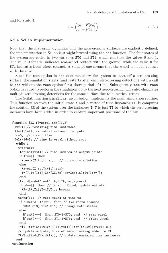
5.2 Modeling and Simulation of a Car 139
and for state 4,
s =(
y0 − F (x0)y1 − F (x1)
). (5.35)
5.2.4 Scilab Implementation
Now that the first-order dynamics and the zero-crossing surfaces are explicitly defined,the implementation in Scilab is straightforward using the ode function. The four states ofthe system are coded in two variables ST0 and ST1, which can take the values 0 and 1.The value 0 for ST0 indicates rear-wheel contact with the ground, while the value 0 forST1 indicates front-wheel contact. A value of one means that the wheel is not in contactwith the road.
Since the root option in ode does not allow the system to start off a zero-crossingsurface, the simulation starts (and restarts after each zero-crossing detection) with a callto ode without the root option for a short period of time. Subsequently, ode with rootoption is called to perform the simulation up to the next zero-crossing. This also eliminatesmultiple zero-crossing detections for the same surface due to numerical errors.
The Scilab function simul car, given below, implements the main simulation routine.This function receives the initial state X and a vector of time instances TT. It computesthe solution XX of the system over the instances T. T is just TT to which the zero crossinginstances have been added in order to capture important positions of the car.
function [XX,T]=simul_car(TT,X)
Tt=TT; // remaining time instances
XX=[];T=[]; // intialization of outputs
tc=0; //current time
delt=1d-3; // time interval without root
while 1
t=tc+delt;
It=find(Tt<t); // find indices of output points
if It==[] thenxt=ode(X,tc,t,car); // no root simulation
elseXx=ode(X,tc,Tt(It),car);
T=[T,Tt(It)];XX=[XX,Xx];xt=Xx(:,$);Tt(It)=[];
end[Xx,rd]=ode(’root’,xt,t,Tt,car,2,carg);
if rd==[] then // no root found, update outputs
XX=[XX,Xx];T=[T,Tt]; break;endtc=rd(1); // root found at time tc
if size(rd,’*’)==3 then // two roots crossed
ST0=1-ST0;ST1=1-ST1; // change both states
elseif rd(2)==1 then ST0=1-ST0; end // rear wheel
if rd(2)==2 then ST1=1-ST1; end // front wheel
endT=[T,Tt(find(Tt<rd(1))),rd(1)];XX=[XX,Xx];X=Xx(:,$);
// update outputs, time of zero-crossing added to TT
Tt=Tt(find(Tt>rd(1))); // update remaining time instances
endendfunction
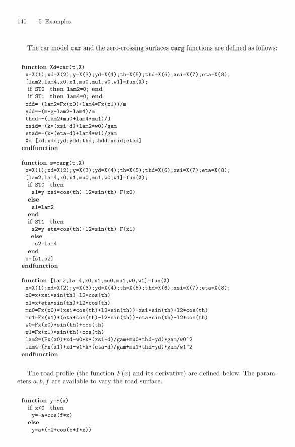
140 5 Examples
The car model car and the zero-crossing surfaces carg functions are defined as follows:
function Xd=car(t,X)
x=X(1);xd=X(2);y=X(3);yd=X(4);th=X(5);thd=X(6);xsi=X(7);eta=X(8);
[lam2,lam4,x0,x1,mu0,mu1,w0,w1]=fun(X);
if ST0 then lam2=0; endif ST1 then lam4=0; endxdd=-(lam2*Fx(x0)+lam4*Fx(x1))/m
ydd=-(m*g-lam2-lam4)/m
thdd=-(lam2*mu0+lam4*mu1)/J
xsid=-(k*(xsi-d)+lam2*w0)/gam
etad=-(k*(eta-d)+lam4*w1)/gam
Xd=[xd;xdd;yd;ydd;thd;thdd;xsid;etad]
endfunction
function s=carg(t,X)
x=X(1);xd=X(2);y=X(3);yd=X(4);th=X(5);thd=X(6);xsi=X(7);eta=X(8);
[lam2,lam4,x0,x1,mu0,mu1,w0,w1]=fun(X);
if ST0 thens1=y-xsi*cos(th)-l2*sin(th)-F(x0)
elses1=lam2
endif ST1 thens2=y-eta*cos(th)+l2*sin(th)-F(x1)
elses2=lam4
ends=[s1,s2]
endfunction
function [lam2,lam4,x0,x1,mu0,mu1,w0,w1]=fun(X)
x=X(1);xd=X(2);y=X(3);yd=X(4);th=X(5);thd=X(6);xsi=X(7);eta=X(8);
x0=x+xsi*sin(th)-l2*cos(th)
x1=x+eta*sin(th)+l2*cos(th)
mu0=Fx(x0)*(xsi*cos(th)+l2*sin(th))-xsi*sin(th)+l2*cos(th)
mu1=Fx(x1)*(eta*cos(th)-l2*sin(th))-eta*sin(th)-l2*cos(th)
w0=Fx(x0)*sin(th)+cos(th)
w1=Fx(x1)*sin(th)+cos(th)
lam2=(Fx(x0)*xd-w0*k*(xsi-d)/gam+mu0*thd-yd)*gam/w0^2
lam4=(Fx(x1)*xd-w1*k*(eta-d)/gam+mu1*thd-yd)*gam/w1^2
endfunction
The road profile (the function F (x) and its derivative) are defined below. The param-eters a, b, f are available to vary the road surface.
function y=F(x)
if x<0 theny=-a*cos(f*x)
elsey=a*(-2+cos(b*f*x))
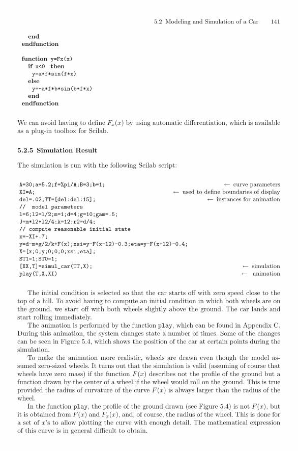
5.2 Modeling and Simulation of a Car 141
endendfunction
function y=Fx(x)
if x<0 theny=a*f*sin(f*x)
elsey=-a*f*b*sin(b*f*x)
endendfunction
We can avoid having to define Fx(x) by using automatic differentiation, which is availableas a plug-in toolbox for Scilab.
5.2.5 Simulation Result
The simulation is run with the following Scilab script:
A=30;a=5.2;f=%pi/A;B=3;b=1; ← curve parametersXI=A; ← used to define boundaries of displaydel=.02;TT=[del:del:15]; ← instances for animation// model parameters
l=6;l2=l/2;m=1;d=4;g=10;gam=.5;
J=m*l2*l2/4;k=12;r2=d/4;
// compute reasonable initial state
x=-XI+.7;
y=d-m*g/2/k+F(x);xsi=y-F(x-l2)-0.3;eta=y-F(x+l2)-0.4;
X=[x;0;y;0;0;0;xsi;eta];
ST1=1;ST0=1;
[XX,T]=simul_car(TT,X); ← simulationplay(T,X,XI) ← animation
The initial condition is selected so that the car starts off with zero speed close to thetop of a hill. To avoid having to compute an initial condition in which both wheels are onthe ground, we start off with both wheels slightly above the ground. The car lands andstart rolling immediately.
The animation is performed by the function play, which can be found in Appendix C.During this animation, the system changes state a number of times. Some of the changescan be seen in Figure 5.4, which shows the position of the car at certain points during thesimulation.
To make the animation more realistic, wheels are drawn even though the model as-sumed zero-sized wheels. It turns out that the simulation is valid (assuming of course thatwheels have zero mass) if the function F (x) describes not the profile of the ground but afunction drawn by the center of a wheel if the wheel would roll on the ground. This is trueprovided the radius of curvature of the curve F (x) is always larger than the radius of thewheel.
In the function play, the profile of the ground drawn (see Figure 5.4) is not F (x), butit is obtained from F (x) and Fx(x), and, of course, the radius of the wheel. This is done fora set of x’s to allow plotting the curve with enough detail. The mathematical expressionof this curve is in general difficult to obtain.
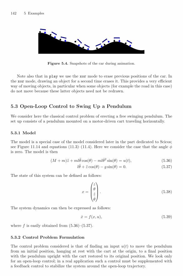
142 5 Examples
Figure 5.4. Snapshots of the car during animation.
Note also that in play we use the xor mode to erase previous positions of the car. Inthe xor mode, drawing an object for a second time erases it. This provides a very efficientway of moving objects, in particular when some objects (for example the road in this case)do not move because these latter objects need not be redrawn.
5.3 Open-Loop Control to Swing Up a Pendulum
We consider here the classical control problem of erecting a free swinging pendulum. Theset up consists of a pendulum mounted on a motor-driven cart traveling horizontally.
5.3.1 Model
The model is a special case of the model considered later in the part dedicated to Scicos;see Figure 11.14 and equations (11.3)–(11.4). Here we consider the case that the angle φis zero. The model is then
(M + m)z + mlθ cos(θ) − mlθ2 sin(θ) = u(t), (5.36)lθ + z cos(θ) − g sin(θ) = 0. (5.37)
The state of this system can be defined as follows:
x =
⎛⎜⎜⎝
zθz
θ
⎞⎟⎟⎠ . (5.38)
The system dynamics can then be expressed as follows:
x = f(x, u), (5.39)
where f is easily obtained from (5.36)–(5.37).
5.3.2 Control Problem Formulation
The control problem considered is that of finding an input u(t) to move the pendulumfrom an initial position, hanging at rest with the cart at the origin, to a final positionwith the pendulum upright with the cart restored to its original position. We look onlyfor an open-loop control; in a real application such a control must be supplemented witha feedback control to stabilize the system around the open-loop trajectory.
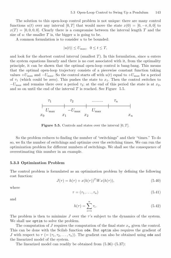
5.3 Open-Loop Control to Swing Up a Pendulum 143
The solution to this open-loop control problem is not unique: there are many controlfunctions u(t) over any interval [0, T ] that would move the state x(0) = [0,−π, 0, 0] tox(T ) = [0, 0, 0, 0]. Clearly there is a compromise between the interval length T and thesize of u: the smaller T is, the bigger u is going to be.
A common formulation is to consider u to be bounded:
|u(t)| ≤ Umax, 0 ≤ t ≤ T,
and look for the shortest control interval (smallest T ). In this formulation, since u entersthe system equations linearly and there is no cost associated with it, from the optimalityprinciple, it can be shown that the optimal open-loop control is bang-bang. This meansthat the optimal open-loop trajectory consists of a piecewise constant function takingvalues +Umax and −Umax. So the control starts off with u(t) equal to +Umax for a periodof τ1 (which could be zero). This pushes the state to x1. Then the control switches to−Umax and remains there over a period τ2; at the end of this period the state is at x2,and so on until the end of the interval T is reached. See Figure 5.5.
.........
−Umax UmaxUmaxx0 x1 x2 xn
τ1 τ2 τn
Figure 5.5. Controls and states over the interval [0, T ].
So the problem reduces to finding the number of “switchings” and their “times.” To doso, we fix the number of switchings and optimize over the switching times. We can run theoptimization problem for different numbers of switchings. We shall see the consequence ofoverestimating this number in an example.
5.3.3 Optimization Problem
The control problem is formulated as an optimization problem by defining the followingcost function:
J(τ) = h(τ) + x(h(τ))T Wx(h(τ)), (5.40)
whereτ = (τ1, . . . , τn) (5.41)
and
h(τ) =n∑
i=1
τi. (5.42)
The problem is then to minimize J over the τ ’s subject to the dynamics of the system.We shall use optim to solve the problem.
The computation of J requires the computation of the final state xn given the control.This can be done with the Scilab function ode. But optim also requires the gradient ofJ with respect to τ (= (τ1, τ2, . . . , τn)). The gradient can also be obtained using ode andthe linearized model of the system.
The linearized model can readily be obtained from (5.36)–(5.37):
144 5 Examples
(M + m)δz − mlθ sin(θ)δθ + ml cos(θ)δθ − mlθ2 cos(θ)δθ − 2mlθ sin(θ)δθ = δu,
lδθ + cos(θ)δz − z sin(θ)δθ − g cos(θ)δθ = 0.
By straightforward algebra, it can be shown that the linearized model can be expressedas follows:
˙δx = A(x, x, u)δx, (5.43)
where
A(x, x, u) =(
0 IV −1F V −1G
)(5.44)
where
F =(
0 ml sin(θ)θ + mlθ2 cos(θ)0 z sin(θ) + g cos(θ)
), (5.45)
G =(
0 2mlθ sin(θ)0 0
), (5.46)
V =(
M + m ml cos(θ)cos(θ) l
). (5.47)
Note that z, θ, and their derivatives are all functions of u.Note also that
∂J
∂τ=
∂h
∂τ+ x(h)T W
∂x(h)∂τ
. (5.48)
∂h∂τ is simply a vector of ones. ∂x(h)
∂τ is the variation in the final state xn due to a variationin τ . Thus we can compute it by computing δxn due to variations δτ .
Let Ψ(t) be the fundamental solution of the linear system (5.43), i.e., the solution ofthe following equation:
Ψ = A(x, x, u)Ψ, Ψ(0) = I. (5.49)
It is then straightforward to see that
δx1 = f(x1, Umax)δτ1, (5.50)δx2 = Ψ(τ2)δx1 + f(x2,−Umax)δτ2 = Ψ(τ2)f(x1, Umax)δτ1 + f(x2,−Umax)δτ2
=(Ψ(τ2)f(x1, Umax) f(x2,−Umax)
) (δτ1
δτ2
). (5.51)
By continuing the same way, we can show that for all i > 0,
δxi = Gi
⎛⎜⎝
δτ1
...δτi
⎞⎟⎠ (5.52)
where G is obtained from the following recursion:
Gi+1 =(Ψ(τi)Gi f(xi, (−1)i+1Umax)
), G0 = [ ]. (5.53)
So at the end we haveδxn = Gnδτ, (5.54)
which allows us to evaluate ∂J∂τ thanks to (5.48):
∂J
∂τ= 1 + xT
n WGn, (5.55)
where 1 denotes a row vector of ones of size n.
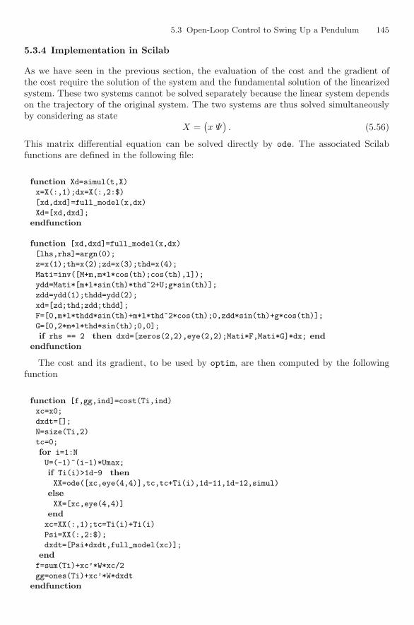
5.3 Open-Loop Control to Swing Up a Pendulum 145
5.3.4 Implementation in Scilab
As we have seen in the previous section, the evaluation of the cost and the gradient ofthe cost require the solution of the system and the fundamental solution of the linearizedsystem. These two systems cannot be solved separately because the linear system dependson the trajectory of the original system. The two systems are thus solved simultaneouslyby considering as state
X =(x Ψ
). (5.56)
This matrix differential equation can be solved directly by ode. The associated Scilabfunctions are defined in the following file:
function Xd=simul(t,X)
x=X(:,1);dx=X(:,2:$)
[xd,dxd]=full_model(x,dx)
Xd=[xd,dxd];
endfunction
function [xd,dxd]=full_model(x,dx)
[lhs,rhs]=argn(0);
z=x(1);th=x(2);zd=x(3);thd=x(4);
Mati=inv([M+m,m*l*cos(th);cos(th),l]);
ydd=Mati*[m*l*sin(th)*thd^2+U;g*sin(th)];
zdd=ydd(1);thdd=ydd(2);
xd=[zd;thd;zdd;thdd];
F=[0,m*l*thdd*sin(th)+m*l*thd^2*cos(th);0,zdd*sin(th)+g*cos(th)];
G=[0,2*m*l*thd*sin(th);0,0];
if rhs == 2 then dxd=[zeros(2,2),eye(2,2);Mati*F,Mati*G]*dx; endendfunction
The cost and its gradient, to be used by optim, are then computed by the followingfunction
function [f,gg,ind]=cost(Ti,ind)
xc=x0;
dxdt=[];
N=size(Ti,2)
tc=0;
for i=1:N
U=(-1)^(i-1)*Umax;
if Ti(i)>1d-9 thenXX=ode([xc,eye(4,4)],tc,tc+Ti(i),1d-11,1d-12,simul)
elseXX=[xc,eye(4,4)]
endxc=XX(:,1);tc=Ti(i)+Ti(i)
Psi=XX(:,2:$);
dxdt=[Psi*dxdt,full_model(xc)];
endf=sum(Ti)+xc’*W*xc/2
gg=ones(Ti)+xc’*W*dxdt
endfunction

146 5 Examples
The main Scilab script which uses optim is the following
�−→ W=100*eye(4,4); // weighing matrix
�−→ M=1;m=.2;l=.6;g=10; // model parameters
�−→ N=5; // number of tau’s
�−→ delt=1.7;T0=ones(1,N)*delt/N; // initial guess
�−→ x0=[0;-%pi;0;0]; // intial state
�−→ Umax=9.7;
�−→ [J,Topt,gr]=optim(cost,’b’,ones(T0)*delt*0,delt*ones(T0),T
0,’ar’,300);
�−→ Topt
Topt =
! 0. 0.2817765 0.6133068 0.5066828 0.1752807 !
Note that we have let n be 5 (maximum of four switchings) but the optimal solutionobtained by optim sets τ1 to zero (Scilab variable Topt contains the vector τ). So thissolution starts off with u = Umax and switches three times over the interval. Both thesimulation result and the animation show that the solution is correct; see Figures 5.6 and5.7.
0.0 0.2 0.4 0.6 0.8 1.0 1.2 1.4 1.6−0.8−0.6−0.4−0.20.00.20.4
0.0 0.2 0.4 0.6 0.8 1.0 1.2 1.4 1.6−4.0−3.5−3.0−2.5−2.0−1.5−1.0−0.5−0.0
0.0 0.2 0.4 0.6 0.8 1.0 1.2 1.4 1.6−10
−8−6−4−202468
10
0.0 0.2 0.4 0.6 0.8 1.0 1.2 1.4 1.6−4−202468
Figure 5.6. The first two figures illustrate the evolution of z and θ. The third figure is thecontrol. The last figure contains the derivatives of z and θ showing that the pendulum comes torest at the end of the interval as required.
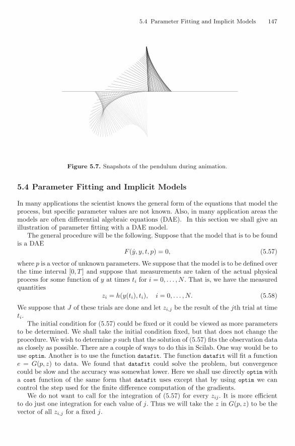
5.4 Parameter Fitting and Implicit Models 147
Figure 5.7. Snapshots of the pendulum during animation.
5.4 Parameter Fitting and Implicit Models
In many applications the scientist knows the general form of the equations that model theprocess, but specific parameter values are not known. Also, in many application areas themodels are often differential algebraic equations (DAE). In this section we shall give anillustration of parameter fitting with a DAE model.
The general procedure will be the following. Suppose that the model that is to be foundis a DAE
F (y, y, t, p) = 0, (5.57)
where p is a vector of unknown parameters. We suppose that the model is to be defined overthe time interval [0, T ] and suppose that measurements are taken of the actual physicalprocess for some function of y at times ti for i = 0, . . . , N . That is, we have the measuredquantities
zi = h(y(ti), ti), i = 0, . . . , N. (5.58)
We suppose that J of these trials are done and let zi,j be the result of the jth trial at timeti.
The initial condition for (5.57) could be fixed or it could be viewed as more parametersto be determined. We shall take the initial condition fixed, but that does not change theprocedure. We wish to determine p such that the solution of (5.57) fits the observation dataas closely as possible. There are a couple of ways to do this in Scilab. One way would be touse optim. Another is to use the function datafit. The function datafit will fit a functione = G(p, z) to data. We found that datafit could solve the problem, but convergencecould be slow and the accuracy was somewhat lower. Here we shall use directly optim witha cost function of the same form that datafit uses except that by using optim we cancontrol the step used for the finite difference computation of the gradients.
We do not want to call for the integration of (5.57) for every zij . It is more efficientto do just one integration for each value of j. Thus we will take the z in G(p, z) to be thevector of all zi,j for a fixed j.
148 5 Examples
5.4.1 Mathematical Model
Many applications use polynomial models. In some cases these are argued for on firstprinciples. In other applications they occur because if linear equations do not suffice, thenthe next natural thing to try is a polynomial equation. If a linear approximation is notadequate, then the next level of Taylor approximation uses quadratic functions. The DAEwe consider arises as the model of a batch reactor and is sometimes used as a test problemin the chemical engineering literature [17, 31]. The equations are
y1 = −p3y2y8, (5.59a)y2 = −p1y2y6 + p2y10 − p3y2y8, (5.59b)y3 = p3y2y8 + p4y4y6 − p5y9, (5.59c)y4 = −p4y4y6 + p5y9, (5.59d)y5 = p1y2y6 − p2y10, (5.59e)y6 = −p1y2y6 − p4y4y6 + p2y10 + p5y9 (5.59f)0 = −0.0131 + y6 + y8 + y9 + y10 − y7, (5.59g)0 = p7y1 − y8(p7 + y7), (5.59h)0 = p8y3 − y9(p8 + y7), (5.59i)0 = p6y5 − y10(p6 + y7). (5.59j)
In its original form this problem is known to be very stiff and is used for a test problemfor parameter sensitivity software. We shall take a slightly modified set of initial conditions.
5.4.2 Scilab Implementation
To illustrate the procedure we shall proceed as follows. Our observational data will begiven by a simulation followed by the addition of random perturbations. We begin with afixed value of p, which we denote by ptrue. Assuming that p is given in the current Scilabenvironment, the system is coded as follows:
function [r,ires]=reactor(t,y,ydot)
ires=0;
r(1)=ydot(1)+p(3)*y(2)*y(8);
r(2)=ydot(2)+p(1)*y(2)*y(6)-p(2)*y(10)+p(3)*y(2)*y(8);
r(3)=ydot(3)-p(3)*y(2)*y(8)-p(4)*y(4)*y(6)+p(5)*y(9);
r(4)=ydot(4)+p(4)*y(4)*y(6)-p(5)*y(9);
r(5)=ydot(5)-p(1)*y(2)*y(6)+p(2)*y(10);
r(6)=ydot(6)+p(1)*y(2)*y(6)+p(4)*y(4)*y(6)-p(2)*y(10)-p(5)*y(9);
r(7)=-0.0131+y(6)+y(8)+y(9)+y(10)-y(7);
r(8)=p(7)*y(1)-y(8)*(p(7)+y(7));
r(9)=p(8)*y(3)-y(9)*(p(8)+y(7));
r(10)=p(6)*y(5)-y(10)*(p(6)+y(7));
endfunction
Since the model (5.59) is a DAE, only some initial conditions will be consistent. Weshall assume that {p6, p7, p8} are known and fixed at the values ptrue(6:8). In this casethe space of consistent initial conditions is independent of the remaining values of pi andwe do not have to worry about finding new consistent initial conditions as the parametersare varied.
5.4 Parameter Fitting and Implicit Models 149
We take fixed initial values of the first 6 components of the initial condition y(0). Theremaining values of y(0) are found by solving the last four equations in (5.59) using fsolve.This ensures that our y(0) is consistent to high order.
�−→ ptrue=[21.893;2.14e3;32.318;21.893;1.07e3;6.65e-3;4.03e-4;5.e-5/32];
�−→ function z=constraints(y2) ← compute constraints for y=[y1,y2]
�−→ r = reactor(0,[y1;y2],0*ones(10,1));
�−→ z = r(7:10);
�−→ endfunction
�−→ function [y,v]=initial_condition(y1) ← compatible initial value given y1
�−→ [y2,v]=fsolve(zeros(4,1),constraints);
�−→ y =[y1;y2];
�−→ endfunction
�−→ y01=[1.5776;8.32;0;0;0;0]; ← initial value of first 6 components�−→ p=ptrue;
�−→ [y0,v]=initial_condition(y01); ← a consistent initial condition�−→ norm(v) ← test consistency
ans =
2.262D-17
Simulations with dassl using y(0) and ptrue show that the solutions are close to steadystate by around t = 0.5. Accordingly we will take our observations on the interval [0, 0.5].These simulations, which are indicated by the solid unmarked lines in Figs. 5.8–5.13, alsoshow that the components of yi vary greatly in size. A given experiment will consist ofobserving the value of the first six components of y every 0.05 seconds for a total of 10 timepoints. Hence the observation times are tts=0.05:0.05:0.5. We generate the experimentaloutcomes by taking a simulation using ptrue and then perturbing the entries by a uniformlygenerated random vector. The perturbations are scaled so that they are of the same relativesize for each entry and each observation time. We take 9 such observations so that J = 9.
�−→ t0=0; tt=0:0.05:0.5;
�−→ y=dassl(y0,t0,tt,reactor); ← integration with p=ptrue
�−→ y=y(2:7,2:11);y(4:6,:)=100*y(4:6,:); ← rescale y(4:6,:)
�−→ rtrue=y(:);
�−→ rand(’seed’,20);
�−→ N=9; ← generate 9 observations perturbed with noise�−→ obs= rtrue*ones(1,N);
�−→ obs= obs.*(1+ 0.1*(rand(60,N,’u’)-0.5)); ← perturbations are to be rela-← tive to the size of what is being perturbed
We then make an intial guess p0 for the first 5 parameters and use optim to find thevalues of {p1, . . . , p5} to best fit the data. The final estimate is denoted by pest. This laststep is carried out now by
�−→ function e=G(p1) ← error function to be minimized
150 5 Examples
�−→ p=[p1;ptrue(6:$)] ← p(6:8) is fixed and fit using p(1:5)
�−→ rr=dassl(y0,t0,tt,1.e-10,1.e-12,reactor);
�−→ rr=rr(2:7,2:11);rr(4:6,:)=100*rr(4:6,:);
�−→ rr=rr(:);
�−→ e=0;
�−→ for i=1:size(obs,’c’)
�−→ gg = (rr-obs(:,i));
�−→ e = e + gg’*gg;
�−→ end�−→ endfunction
�−→ function [f,g,ind]=costf(p,ind) ← cost function for optim
�−→ if ind==2|ind==4 then�−→ f=G(p);
�−→ else�−→ f=0;
�−→ end;�−→ if ind==3|ind==4 then�−→ g=0*p;
�−→ pa=sqrt(%eps)*10*abs(p);
�−→ f=G(p);
�−→ for j=1:size(p,’*’) do
�−→ v=0*p;v(j)=pa(j),
�−→ g(j)=(G(p+v)-f)/v(j);
�−→ end;�−→ else�−→ g=0*p;
�−→ end�−→ endfunction
�−→ p0=ptrue(1:5)*0.5; ← initial guess for p
�−→ [err,pest]=optim(costf,p0,’ar’,100,100,1.e-9,1.e-9,imp=2);
�−→ [p0,pest,ptrue(1:5)] ← fitted parametersans =
! 10.9465 10.614308 21.893 !
! 1070. 1105.6571 2140. !
! 16.159 33.346866 32.318 !
! 10.9465 5.8412889 21.893 !
! 535. 946.85234 1070. !
�−→ [G(p0),G(pest),G(ptrue(1:5))] ← cost minimized by datafit
ans =
! 453.75872 6.1442786 5.2443056 !
The first thing one notices is that pest is not the same as ptrue(1:5), nor is it evenvery close. However, if we examine the answer we see that we have in fact found a goodapproximation. Running the following script will graph the different yi for p0, ptrue, andpest. What we see is that the new value pest is providing a good fit to the data. Thisexample shows the importance of using parameter bounds whenever they are available
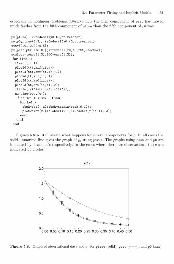
5.4 Parameter Fitting and Implicit Models 151
especially in nonlinear problems. Observe how the fifth component of pest has movedmuch farther from the fifth component of ptrue than the fifth component of p0 was.
p=[ptrue]; krt=dassl(y0,t0,tt,reactor);
p=[p0;ptrue(6:$)];kr0=dassl(y0,t0,tt,reactor);
ttt=[0.01:0.02:0.5];
p=[pest;ptrue(6:$)];krf=dassl(y0,t0,ttt,reactor);
scale_r=[ones(1,3),100*ones(1,3)];
for ii=2:11
f1=scf(ii-1);
plot2d(ttt,krf(ii,:));
plot2d(ttt,krf(ii,:),-1);
plot2d(tt,krt(ii,:));
plot2d(tt,kr0(ii,:));
plot2d(tt,kr0(ii,:),-2);
xtitle(’y(’+string(ii-1)+’)’);
nz=size(obs,’c’);
if nz <>1 & ii<=7 thenfor k=1:N
obsk=obs(:,k);obsk=matrix(obsk,6,10);
plot2d(tt(2:$)’,obsk(ii-1,:)./scale_r(ii-1),-3);
endend
end
Figures 5.8–5.13 illustrate what happens for several components for y. In all cases thesolid unmarked line gives the graph of yi using ptrue. The graphs using pest and p0 areindicated by + and ×’s respectively. In the cases where there are observations, those areindicated by circles.
y(1)
0.00 0.05 0.10 0.15 0.20 0.25 0.30 0.35 0.40 0.45 0.500.0
0.5
1.0
1.5
2.0
Figure 5.8. Graph of observational data and y1 for ptrue (solid), pest (+++), and p0 (xxx).
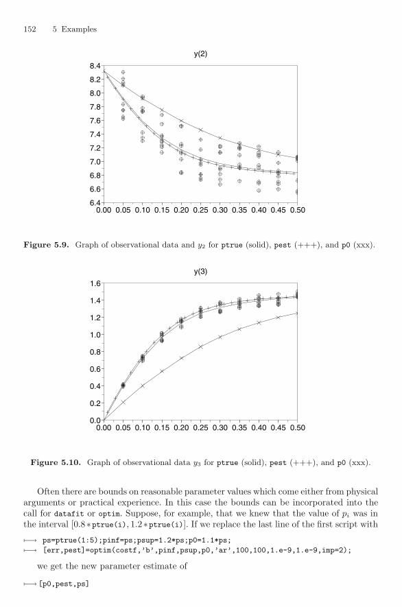
152 5 Examples
y(2)
0.00 0.05 0.10 0.15 0.20 0.25 0.30 0.35 0.40 0.45 0.506.4
6.6
6.8
7.0
7.2
7.4
7.6
7.8
8.0
8.2
8.4
Figure 5.9. Graph of observational data and y2 for ptrue (solid), pest (+++), and p0 (xxx).
y(3)
0.00 0.05 0.10 0.15 0.20 0.25 0.30 0.35 0.40 0.45 0.500.0
0.2
0.4
0.6
0.8
1.0
1.2
1.4
1.6
Figure 5.10. Graph of observational data y3 for ptrue (solid), pest (+++), and p0 (xxx).
Often there are bounds on reasonable parameter values which come either from physicalarguments or practical experience. In this case the bounds can be incorporated into thecall for datafit or optim. Suppose, for example, that we knew that the value of pi was inthe interval [0.8∗ptrue(i), 1.2∗ptrue(i)]. If we replace the last line of the first script with
�−→ ps=ptrue(1:5);pinf=ps;psup=1.2*ps;p0=1.1*ps;
�−→ [err,pest]=optim(costf,’b’,pinf,psup,p0,’ar’,100,100,1.e-9,1.e-9,imp=2);
we get the new parameter estimate of
�−→ [p0,pest,ps]
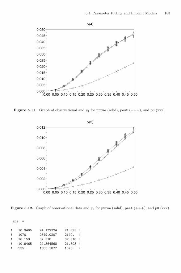
5.4 Parameter Fitting and Implicit Models 153
y(4)
0.00 0.05 0.10 0.15 0.20 0.25 0.30 0.35 0.40 0.45 0.500.000
0.005
0.010
0.015
0.020
0.025
0.030
0.035
0.040
0.045
0.050
Figure 5.11. Graph of observational and y4 for ptrue (solid), pest (+++), and p0 (xxx).
y(5)
0.00 0.05 0.10 0.15 0.20 0.25 0.30 0.35 0.40 0.45 0.500.000
0.002
0.004
0.006
0.008
0.010
0.012
Figure 5.12. Graph of observational data and y5 for ptrue (solid), pest (+++), and p0 (xxx).
ans =
! 10.9465 24.172324 21.893 !
! 1070. 2349.0207 2140. !
! 16.159 32.318 32.318 !
! 10.9465 24.364568 21.893 !
! 535. 1083.1877 1070. !
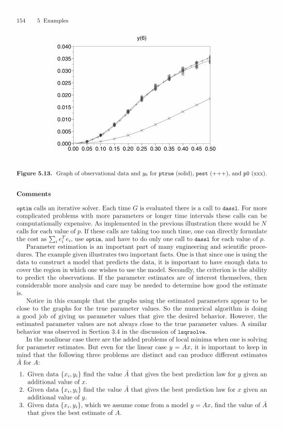
154 5 Examples
y(6)
0.00 0.05 0.10 0.15 0.20 0.25 0.30 0.35 0.40 0.45 0.500.000
0.005
0.010
0.015
0.020
0.025
0.030
0.035
0.040
Figure 5.13. Graph of observational data and y6 for ptrue (solid), pest (+++), and p0 (xxx).
Comments
optim calls an iterative solver. Each time G is evaluated there is a call to dassl. For morecomplicated problems with more parameters or longer time intervals these calls can becomputationally expensive. As implemented in the previous illustration there would be Ncalls for each value of p. If these calls are taking too much time, one can directly formulatethe cost as
∑i eT
i ei, use optim, and have to do only one call to dassl for each value of p.Parameter estimation is an important part of many engineering and scientific proce-
dures. The example given illustrates two important facts. One is that since one is using thedata to construct a model that predicts the data, it is important to have enough data tocover the region in which one wishes to use the model. Secondly, the criterion is the abilityto predict the observations. If the parameter estimates are of interest themselves, thenconsiderable more analysis and care may be needed to determine how good the estimateis.
Notice in this example that the graphs using the estimated parameters appear to beclose to the graphs for the true parameter values. So the numerical algorithm is doinga good job of giving us parameter values that give the desired behavior. However, theestimated parameter values are not always close to the true parameter values. A similarbehavior was observed in Section 3.4 in the discussion of lsqrsolve.
In the nonlinear case there are the added problems of local minima when one is solvingfor parameter estimates. But even for the linear case y = Ax, it is important to keep inmind that the following three problems are distinct and can produce different estimatesA for A:
1. Given data {xi, yi} find the value A that gives the best prediction law for y given anadditional value of x.
2. Given data {xi, yi} find the value A that gives the best prediction law for x given anadditional value of y.
3. Given data {xi, yi}, which we assume come from a model y = Ax, find the value of Athat gives the best estimate of A.
5.4 Parameter Fitting and Implicit Models 155
The functions optim, datafit, and lsqrsolve as described here are being used for the firsttype of problem since the error in the value of G is being minimized. The function G needsto be formulated differently if either problem 2 or 3 is to be solved.
Finally, this example illustrates an important aspect of solving optimization problems.Finding the optimal solution even when we know it exists can be difficult. When we initiallysolved this problem we used more of the default settings of optim and dassl. The resultwas not nearly as good as reported above. After some experimentation, it was determinedthat one factor was that the gradient approximation was not accurate enough. Since thefunction being differenced was the result of an integration by dassl, we both increasedthe lower bound on the difference in optim and tightened the error tolerances in dassl.Another problem was that the large difference in magnitude of the components was leadingto inaccuracy. So we put a factor of 100 in the function evaluation, which helps preventstagnation and increased accuracy of gradients. In particular, we rescaled y(4:6) to givethese variables a range similar to those in y(1:3). This was necessary to increase the partdedicated to y(1:3) in the global cost.
We also gave optim some guidance. In
[err,pest]=optim(costf,p0,’ar’,100,100,1.e-9,1.e-9,imp=2)
the 1.e-9 sets the thresholds on the gradient norm and the decrease in f. Here we areforcing the change in f and the gradient to be rather small at termination since theyneed to be below these thresholds. The imp=2 gives a verbose reporting on the iterations,which was used in examining the behavior of the iteration while deciding where to set thethresholds. In trying to solve a parameter problem in practice when the solution is notknown it is often helpful to try first what we have done here. That is, generate observationsby simulation with known parameters and then try first to find the known parameters. Thishelps in checking that the problem is properly coded and gives insights into the problem’sbehavior. Thus the problem solved in this section is not as academic as it appears and isrepresentative of part of the solution of real problems.
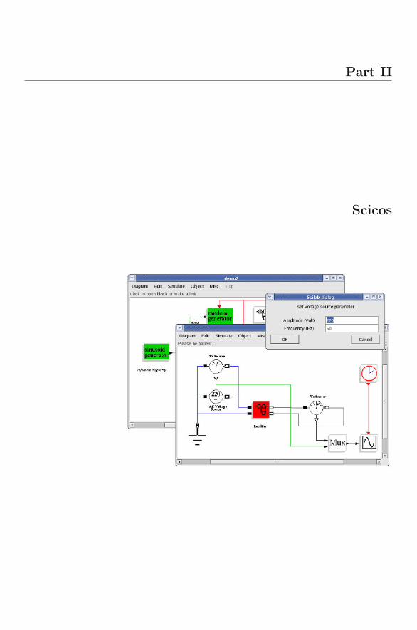
Part II
Scicos
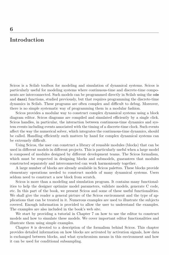
6
Introduction
Scicos is a Scilab toolbox for modeling and simulation of dynamical systems. Scicos isparticularly useful for modeling systems where continuous-time and discrete-time compo-nents are interconnected. Such models can be programmed directly in Scilab using the odeand dassl functions, studied previously, but that requires programming the discrete-timedynamics in Scilab. These programs are often complex and difficult to debug. Moreover,there is no simple systematic way of programming them in a modular fashion.
Scicos provides a modular way to construct complex dynamical systems using a blockdiagram editor. Scicos diagrams are compiled and simulated efficiently by a single click.Scicos handles, in particular, the interaction between continuous-time dynamics and sys-tem events including events associated with the timing of a discrete-time clock. Such eventsaffect the way the numerical solver, which integrates the continuous-time dynamics, shouldbe called. Handling efficiently such matters by hand for complex dynamical systems canbe extremely difficult.
Using Scicos, the user can construct a library of reusable modules (blocks) that can beused in different models in different projects. This is particularly useful when a large modelis composed of modules designed by different development teams. The Scicos formalism,which must be respected in designing blocks and submodels, guarantees that modulesconstructed separately and interconnected can work harmoniously together.
A large number of blocks are already available in Scicos palettes. These blocks provideelementary operations needed to construct models of many dynamical systems. Usersseldom need to construct a new block from scratch.
Scicos is more than a modeling and simulation program. It contains many functional-ities to help the designer optimize model parameters, validate models, generate C code,etc. In this part of the book, we present Scicos and some of these useful functionalities.We shall give the reader a general picture of the Scicos environment and the type of ap-plications that can be treated in it. Numerous examples are used to illustrate the subjectscovered. Enough information is provided to allow the user to understand the examples.The examples are also included in the book’s web site.
We start by providing a tutorial in Chapter 7 on how to use the editor to constructmodels and how to simulate these models. We cover important editor functionalities andillustrate them using simple examples.
Chapter 8 is devoted to a description of the formalism behind Scicos. This chapterprovides detailed information on how blocks are activated by activation signals, how datais exchanged between blocks, and what synchronism means in this environment and howit can be used for conditional subsampling.

160 6 Introduction
Even if in many cases Scicos diagrams can be constructed using existing blocks, some-times it is more convenient, or even becomes necessary, to develop new blocks. This is thesubject of Chapter 9. Sometimes a new block is not absolutely necessary but can simplifythe diagram and/or its use can make the simulation of the diagram more efficient. Variousways of constructing new blocks are discussed in this chapter. The content of this chapter,however, is fairly technical, and most users may skip it on a first reading.
In Chapter 10, through a number of examples, we show what types of systems can bemodeled in Scicos and propose solutions for modeling certain behaviors that are particu-larly difficult to realize outside of Scicos.
Often the objective for modeling and simulation is parameter optimization. The pa-rameter can be a system parameter to be tuned in an identification process, or a controlleror filter parameter to be adjusted to a given system. The procedure for parameter opti-mization consists in associating a cost (obtained by simulation) to a set of parameters.This cost is then optimized by standard optimization techniques. This procedure, whichusually requires many simulation runs, can easily be implemented in the Scilab-Scicos en-vironment by batch processing. In Chapter 11, we present Scilab functions used for batchsimulation of Scicos diagrams in Scilab and present a number of examples illustratingtypical applications.
Code generation is an important functionality in Scicos. A typical application is toa situation in which the diagram models a controlled system. The control part of thediagram, after validation of the control law through simulation, is to be implemented inan embedded system. For that, C code generation can be performed for a part of thediagram designated by the user. Code generation is the subject of Chapter 12. Examplesare provided and some pitfalls are discussed.
A number of debugging functionalities are available in Scicos. They are explained inChapter 13. Debugging is particularly useful when diagrams become complex and whenuser-defined blocks are used. A few examples are provided to show how debugging can bedone efficiently.
A recent addition to Scicos is the capacity to use “implicit” blocks in a Scicos diagram.This allows the construction of systems using blocks modeling physical components ina natural way. These blocks have no explicit inputs and outputs but rather have ports.Connecting these ports by links defines constraints. For example, in this environment wecan define an electrical circuit with implicit blocks modeling resistors, capacitors, diodes,and other electrical components, and with links imposing Kirchoff’s laws of current andequality of voltages at the two connected ports. The possibility to mix implicit and nor-mal blocks in the same environment provides a powerful modeling environment that ispresented in Chapter 14. It should, however, be noted that the implementation of implicitblocks is at the beta testing stage.
Appendix A contains an introduction on how Scicos is implemented and, in particular,what data structures it uses. Understanding implementation issues is very useful not onlyfor advanced users who want to customize the tool, but also for anybody who encounterssubtle modeling problems and wants to take full advantage of debugging facilities. Thischapter also gives a lot of information on where important Scicos programs can be found.Most of these programs (except for the simulator part) are Scilab programs, so they areeasy to read and customize.
In this book we present functionalities of Scicos distributed with Scilab version 3.1 orhigher. Even though most of the discussions apply also to Scicos in Scilab 3.0, some of theexamples may not run on this earlier version.
Note also that running some of the examples presented here requires a C compiler. Thisis usually no problem under Linux, MacOSX, and most Unix workstations. But under the

6 Introduction 161
Windows operating system, it requires the installation of Visual C++. Visual C++ isautomatically instantiated and usable by Scilab if Scilab is run by clicking on its icon.
7
Getting Started
7.1 Construction of a Simple Diagram
Scicos contains a graphical editor that can be used to construct block diagram models ofdynamical systems. The blocks can come from various palettes provided in Scicos or canbe user-defined. In this section, we describe how the editor can be used to construct simplemodels and how these models can be simulated.
7.1.1 Running Scicos
Scicos is a Scilab toolbox included in the Scilab package. The Scicos editor can be openedby the scicos command
�−→ scicos;
This command opens up an empty Scicos diagram named by default Untitled. Calledwith an argument, it can open up an existing diagram:
�−→ scicos my_diagram.cos;
The Scicos main window displaying an empty diagram is illustrated in Figure 7.1. Thelook of the main window may be slightly different under different window managers andoperating systems. Editor functionalities are available through pull-down menus placedat the top of the editor window. The manual page of each functionality is displayed byselecting Help in the Misc menu and then the item of interest in the menu.
Some of the editor functionalities can also be accessed by clicking the right mousebutton. Finally, keyboard shortcuts can be used for various operations. For example, typingan “r” activates the operation Replot, which centers and redraws the diagram. Keyboardshortcuts can be defined by the user.
7.1.2 Editing a Model
To construct a model, we need to access Scicos blocks. Scicos provides many elementaryblocks organized in different palettes that can be accessed using the operation Palettesin the Edit menu. This operation opens up a dialog box that includes the list of availablepalettes. By selecting a palette in the list, a new Scicos window opens up displaying theblocks available in this palette. Figure 7.2 shows the blocks in the Sources palette. Blocksfrom palettes can be copied into the main Scicos window by clicking first on the desiredblock and then at the location where the block is to be copied in the Scicos window.
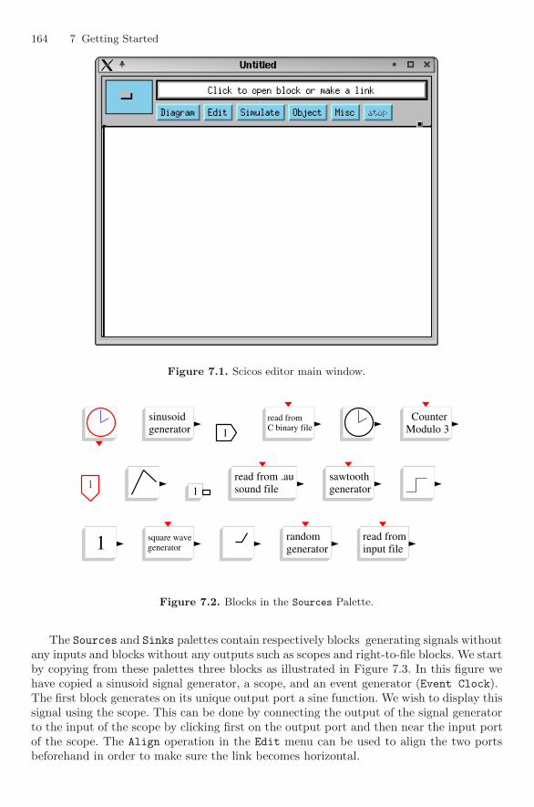
164 7 Getting Started
Figure 7.1. Scicos editor main window.
11 generatorsquare wavegeneratorsquare wave
generatorrandomgeneratorrandom
input fileread frominput fileread from
1111 sound file
read from .ausound fileread from .au
generatorsawtoothgeneratorsawtooth
generatorsinusoidgeneratorsinusoid
11 C binary fileread fromC binary fileread from
Modulo 3 CounterModulo 3 Counter
Figure 7.2. Blocks in the Sources Palette.
The Sources and Sinks palettes contain respectively blocks generating signals withoutany inputs and blocks without any outputs such as scopes and right-to-file blocks. We startby copying from these palettes three blocks as illustrated in Figure 7.3. In this figure wehave copied a sinusoid signal generator, a scope, and an event generator (Event Clock).The first block generates on its unique output port a sine function. We wish to display thissignal using the scope. This can be done by connecting the output of the signal generatorto the input of the scope by clicking first on the output port and then near the input portof the scope. The Align operation in the Edit menu can be used to align the two portsbeforehand in order to make sure the link becomes horizontal.
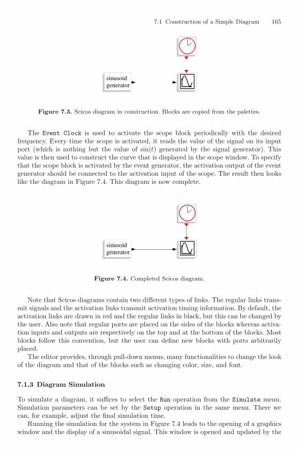
7.1 Construction of a Simple Diagram 165
generatorsinusoidgeneratorsinusoid
Figure 7.3. Scicos diagram in construction. Blocks are copied from the palettes.
The Event Clock is used to activate the scope block periodically with the desiredfrequency. Every time the scope is activated, it reads the value of the signal on its inputport (which is nothing but the value of sin(t) generated by the signal generator). Thisvalue is then used to construct the curve that is displayed in the scope window. To specifythat the scope block is activated by the event generator, the activation output of the eventgenerator should be connected to the activation input of the scope. The result then lookslike the diagram in Figure 7.4. This diagram is now complete.
generatorsinusoidgeneratorsinusoid
Figure 7.4. Completed Scicos diagram.
Note that Scicos diagrams contain two different types of links. The regular links trans-mit signals and the activation links transmit activation timing information. By default, theactivation links are drawn in red and the regular links in black, but this can be changed bythe user. Also note that regular ports are placed on the sides of the blocks whereas activa-tion inputs and outputs are respectively on the top and at the bottom of the blocks. Mostblocks follow this convention, but the user can define new blocks with ports arbitrarilyplaced.
The editor provides, through pull-down menus, many functionalities to change the lookof the diagram and that of the blocks such as changing color, size, and font.
7.1.3 Diagram Simulation
To simulate a diagram, it suffices to select the Run operation from the Simulate menu.Simulation parameters can be set by the Setup operation in the same menu. There wecan, for example, adjust the final simulation time.
Running the simulation for the system in Figure 7.4 leads to the opening of a graphicswindow and the display of a sinusoidal signal. This window is opened and updated by the
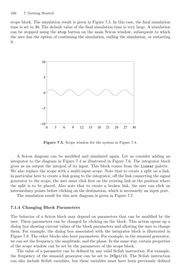
166 7 Getting Started
scope block. The simulation result is given in Figure 7.5. In this case, the final simulationtime is set to 30. The default value of the final simulation time is very large. A simulationcan be stopped using the stop button on the main Scicos window, subsequent to whichthe user has the option of continuing the simulation, ending the simulation, or restartingit.
0 3 6 9 12 15 18 21 24 27 30−10
−5
0
5
10
+
Figure 7.5. Scope window for the system in Figure 7.4.
A Scicos diagram can be modified and simulated again. Let us consider adding anintegrator to the diagram in Figure 7.4 as illustrated in Figure 7.6. The integrator blockgives as an output the integral of its input. This block comes from the Linear palette.We also replace the scope with a multi-input scope. Note that to create a split on a link,in particular here to create a link going to the integrator, off the link connecting the signalgenerator to the scope, the user must click first on the existing link at the position wherethe split is to be placed. Also note that to create a broken link, the user can click onintermediary points before clicking on the destination, which is necessarily an input port.
The simulation result for this new diagram is given in Figure 7.7.
7.1.4 Changing Block Parameters
The behavior of a Scicos block may depend on parameters that can be modified by theuser. These parameters can be changed by clicking on the block. This action opens up adialog box showing current values of the block parameters and allowing the user to changethem. For example, the dialog box associated with the integrator block is illustrated inFigure 7.8. The other blocks also have parameters. For example, in the sinusoid generator,we can set the frequency, the amplitude, and the phase. In the same way, certain propertiesof the scope window can be set by the parameters of the scope block.
The value of a parameter can be defined by any valid Scilab instruction. For example,the frequency of the sinusoid generator can be set to 2*%pi/10. The Scilab instructioncan also include Scilab variables, but these variables must have been previously defined
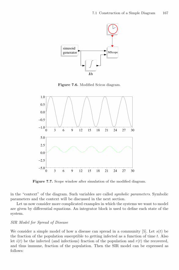
7.1 Construction of a Simple Diagram 167
generatorsinusoidgeneratorsinusoid
1/s
MScopeMScope
Figure 7.6. Modified Scicos diagram.
0 3 6 9 12 15 18 21 24 27 30−1.0
−0.5
0.0
0.5
1.0
+
0 3 6 9 12 15 18 21 24 27 30−5.0
−2.5
0.0
2.5
5.0
+
Figure 7.7. Scope window after simulation of the modified diagram.
in the “context” of the diagram. Such variables are called symbolic parameters. Symbolicparameters and the context will be discussed in the next section.
Let us now consider more complicated examples in which the systems we want to modelare given by differential equations. An integrator block is used to define each state of thesystem.
SIR Model for Spread of Disease
We consider a simple model of how a disease can spread in a community [5]. Let s(t) bethe fraction of the population susceptible to getting infected as a function of time t. Alsolet i(t) be the infected (and infectious) fraction of the population and r(t) the recovered,and thus immune, fraction of the population. Then the SIR model can be expressed asfollows:
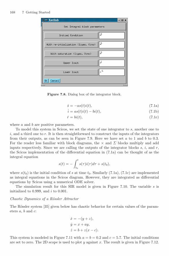
168 7 Getting Started
Figure 7.8. Dialog box of the integrator block.
s = −as(t)i(t), (7.1a)i = as(t)i(t) − bi(t), (7.1b)r = bi(t), (7.1c)
where a and b are positive parameters.To model this system in Scicos, we set the state of one integrator to s, another one to
i, and a third one to r. It is then straightforward to construct the inputs of the integratorsfrom their outputs, as can be seen in Figure 7.9. Here we have set a to 1 and b to 0.3.For the reader less familiar with block diagrams, the × and Σ blocks multiply and addinputs respectively. Since we are calling the outputs of the integrator blocks s, i, and r,the Scicos implementation of the differential equation in (7.1a) can be thought of as theintegral equation
s(t) = −∫ t
t0
s(τ)i(τ)dτ + s(t0),
where s(t0) is the initial condition of s at time t0. Similarly (7.1a), (7.1c) are implementedas integral equations in the Scicos diagram. However, they are integrated as differentialequations by Scicos using a numerical ODE solver.
The simulation result for this SIR model is given in Figure 7.10. The variable s isinitialized to 0.999, and i to 0.001.
Chaotic Dynamics of a Rossler Attractor
The Rossler system [35] given below has chaotic behavior for certain values of the param-eters a, b and c:
x = −(y + z),y = x + ay,
z = b + z(x − c).
This system is modeled in Figure 7.11 with a = b = 0.2 and c = 5.7. The initial conditionsare set to zero. The 2D scope is used to plot y against x. The result is given in Figure 7.12.

7.2 Symbolic Parameters and Context 169
S
I
R
−
−
−
−
−1−1
.3.3
Mux
Figure 7.9. Scicos implementation of the SIR model.
0 3 6 9 12 15 18 21 24 27 300.00
0.25
0.50
0.75
1.00
+
Figure 7.10. The simulation shows, as expected, that the percentage of the recovered populationis increasing and that of the susceptible population is decreasing. The percentage of populationinfected reaches its maximum at a time called the peak of the epidemic.
7.2 Symbolic Parameters and Context
Often it is useful to use symbolic parameters to define block parameters. This is partic-ularly the case if the same parameter is used in more than one block or if the parameteris computed as a function of other parameters. Symbolic parameters are simply Scilabvariables that must be defined in the context of the diagram before being used in thedefinition of block parameters.
Each Scicos diagram contains a context. The context is simply a Scilab script usedto define Scilab variables, which can then be used to define block parameters. To accessthe context of the diagram, use the Context button in the Edit menu. This opens up
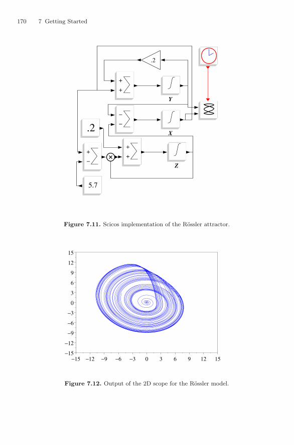
170 7 Getting Started
Y
X
Z
−
−
−
−
+
+
+
+
.2.2
+
+
+
++
−
+
−
5.75.7
.2.2
Figure 7.11. Scicos implementation of the Rossler attractor.
−15 −12 −9 −6 −3 0 3 6 9 12 15−15
−12
−9
−6
−3
0
3
6
9
12
15
+
Figure 7.12. Output of the 2D scope for the Rossler model.
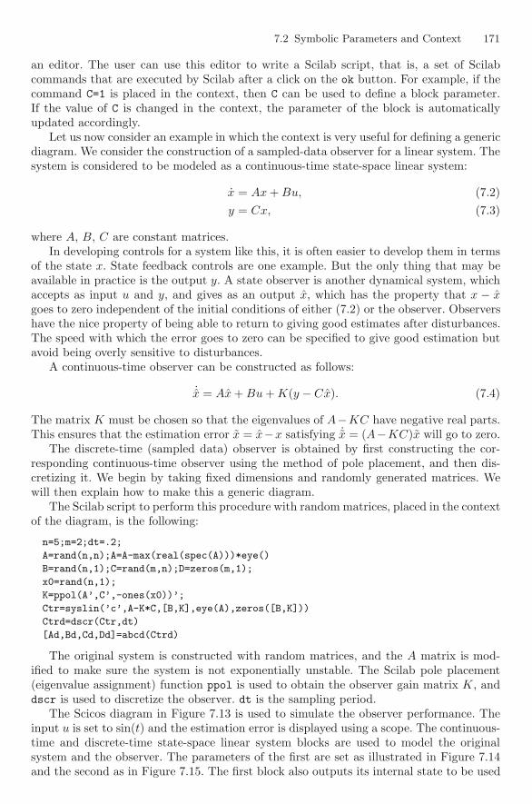
7.2 Symbolic Parameters and Context 171
an editor. The user can use this editor to write a Scilab script, that is, a set of Scilabcommands that are executed by Scilab after a click on the ok button. For example, if thecommand C=1 is placed in the context, then C can be used to define a block parameter.If the value of C is changed in the context, the parameter of the block is automaticallyupdated accordingly.
Let us now consider an example in which the context is very useful for defining a genericdiagram. We consider the construction of a sampled-data observer for a linear system. Thesystem is considered to be modeled as a continuous-time state-space linear system:
x = Ax + Bu, (7.2)y = Cx, (7.3)
where A, B, C are constant matrices.In developing controls for a system like this, it is often easier to develop them in terms
of the state x. State feedback controls are one example. But the only thing that may beavailable in practice is the output y. A state observer is another dynamical system, whichaccepts as input u and y, and gives as an output x, which has the property that x − xgoes to zero independent of the initial conditions of either (7.2) or the observer. Observershave the nice property of being able to return to giving good estimates after disturbances.The speed with which the error goes to zero can be specified to give good estimation butavoid being overly sensitive to disturbances.
A continuous-time observer can be constructed as follows:
˙x = Ax + Bu + K(y − Cx). (7.4)
The matrix K must be chosen so that the eigenvalues of A−KC have negative real parts.This ensures that the estimation error x = x−x satisfying ˙x = (A−KC)x will go to zero.
The discrete-time (sampled data) observer is obtained by first constructing the cor-responding continuous-time observer using the method of pole placement, and then dis-cretizing it. We begin by taking fixed dimensions and randomly generated matrices. Wewill then explain how to make this a generic diagram.
The Scilab script to perform this procedure with random matrices, placed in the contextof the diagram, is the following:
n=5;m=2;dt=.2;
A=rand(n,n);A=A-max(real(spec(A)))*eye()
B=rand(n,1);C=rand(m,n);D=zeros(m,1);
x0=rand(n,1);
K=ppol(A’,C’,-ones(x0))’;
Ctr=syslin(’c’,A-K*C,[B,K],eye(A),zeros([B,K]))
Ctrd=dscr(Ctr,dt)
[Ad,Bd,Cd,Dd]=abcd(Ctrd)
The original system is constructed with random matrices, and the A matrix is mod-ified to make sure the system is not exponentially unstable. The Scilab pole placement(eigenvalue assignment) function ppol is used to obtain the observer gain matrix K, anddscr is used to discretize the observer. dt is the sampling period.
The Scicos diagram in Figure 7.13 is used to simulate the observer performance. Theinput u is set to sin(t) and the estimation error is displayed using a scope. The continuous-time and discrete-time state-space linear system blocks are used to model the originalsystem and the observer. The parameters of the first are set as illustrated in Figure 7.14and the second as in Figure 7.15. The first block also outputs its internal state to be used
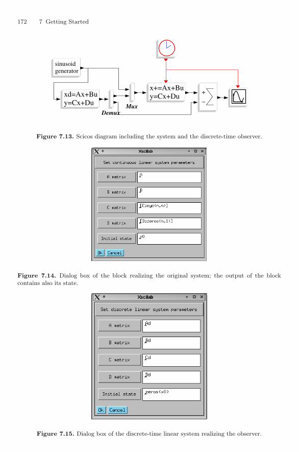
172 7 Getting Started
generatorsinusoidgeneratorsinusoid
y=Cx+Duxd=Ax+Buy=Cx+Duxd=Ax+Bu
Demux
y=Cx+Dux+=Ax+Buy=Cx+Dux+=Ax+Bu
Mux
+
−
+
−
Figure 7.13. Scicos diagram including the system and the discrete-time observer.
Figure 7.14. Dialog box of the block realizing the original system; the output of the blockcontains also its state.
Figure 7.15. Dialog box of the discrete-time linear system realizing the observer.
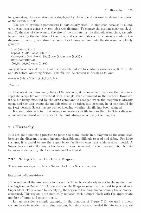
7.3 Hierarchy 173
for generating the estimation error displayed by the scope. dt is used to define the periodof the Event Clock.
The use of symbolic parameters is particularly useful in this case because it allowsus to construct a generic system observer diagram. To change the system matrices A, B,and C, the size of the system, the size of the outputs, or the discretization time, we onlyhave to modify the definition of the m, n, and system matrices. No change is made to thediagram. In fact, by rewriting the context as follows we can make the diagram completelygeneric:
load(’datafile’)
K=ppol(A’,C’,-ones(x0))’;
Ctr=syslin(’c’,A-K*C,[B,K],eye(A),zeros([B,K]))
Ctrd=dscr(Ctr,dt)
[Ad,Bd,Cd,Dd]=abcd(Ctrd)
We just have to make sure that the data file datafile contains variables A, B, C, D, x0,and dt before launching Scicos. This file can be created in Scilab as follows:
�−→ save(’datafile’’,A,B,C,x0,dt)
Remark
If the context contains many lines of Scilab code, it is convenient to place the code in aseparate script file and execute it with a single exec command in the context. However,if the file being executed by the exec command is changed when the diagram is alreadyopen, and the user wants the modification to be taken into account, he or she should doan Eval because Scicos has no way of knowing whether the file has been changed.
It should also be noted that using a separate script file implies that the Scicos diagramis not self-contained and this script file must always accompany the diagram.
7.3 Hierarchy
It is not good modeling practice to place too many blocks in a diagram at the same levelbecause the diagram becomes incomprehensible and difficult to read and debug. For largesystems, it is useful to use the Super block facility to construct a hierarchical model. ASuper block looks like any other block: it can be moved, copied, resized, etc., but itsbehavior is defined by the Scicos submodel within it.
7.3.1 Placing a Super Block in a Diagram
There are two ways to place a Super block in a Scicos diagram.
Region-to-Super-block
If the submodel the user wants to place in a Super block already exists in the model, thenthe Region-to-Super-block operation of the Diagram menu can be used to place it in aSuper block. This is done by specifying the region of the diagram containing the submodelconcerned. This region is automatically replaced with a Super block with the appropriatenumber of input and output ports.
Let us consider a simple example. In the diagram of Figure 7.13, we used a linearsystem block to model the original system, but since we also needed its internal state, we
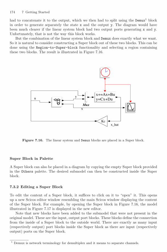
174 7 Getting Started
had to concatenate it to the output, which we then had to split using the Demux1 blockin order to generate separately the state x and the output y. The diagram would havebeen much clearer if the linear system block had two output ports generating x and y.Unfortunately, that is not the way this block works.
But the combination of the linear system block and Demux does exactly what we want.So it is natural to consider constructing a Super block out of these two blocks. This can bedone using the Region-to-Super-block functionality and selecting a region containingthese two blocks. The result is illustrated in Figure 7.16.
y=Cx+Dux+=Ax+Buy=Cx+Dux+=Ax+Bu
KcKc
Muxx
u
x_hat
y
Figure 7.16. The linear system and Demux blocks are placed in a Super block.
Super Block in Palette
A Super block can also be placed in a diagram by copying the empty Super block providedin the Others palette. The desired submodel can then be constructed inside the Superblock.
7.3.2 Editing a Super Block
To edit the content of a Super block, it suffices to click on it to “open” it. This opensup a new Scicos editor window resembling the main Scicos window displaying the contentof the Super block. For example, by opening the Super block in Figure 7.16, the modelillustrated in Figure 7.17 is displayed in the new editor.
Note that new blocks have been added to the submodel that were not present in theoriginal model. These are the input, output port blocks. These blocks define the connectionfrom the inside of a Super block to the outside world. There are exactly as many input(respectively output) port blocks inside the Super block as there are input (respectivelyoutput) ports on the Super block.
1 Demux is network terminology for demultiplex and it means to separate channels.
7.4 Save and Load 175
y=Cx+Duxd=Ax+Buy=Cx+Duxd=Ax+Bu
DemuxSystem
11 11
22
Figure 7.17. Inside the Super block.
The Super block can be edited just like the main Scicos diagram, and when the editingis complete, closing the diagram will commit the changes to the main diagram. If thenumber of input or output port blocks is modified, after closing the Super block, thenumber of ports of the Super block in the main window is adjusted accordingly. Note thatthe port blocks must be numbered consecutively and the corresponding ports on the Superblock are also numbered counting consecutively from the top to the bottom.
Each Super block has a context. The values of symbolic parameters used in the blocksof a Super block are normally defined in the context of the Super block or in the contextof the diagram.
7.4 Save and Load
7.4.1 Scicos File Formats
Scicos diagrams can be saved in two different formats. The most common format is abinary file for which by convention the extension .cos is used. This file is simply a binaryScilab data file and can be loaded in Scilab (assuming its name is myfile.cos) using thecommand
�−→ load myfile.cos
There are three Scilab variables inside .cos files:
• scs m: this Scilab structure contains all the information concerning the diagram• %cpr: this Scilab structure contains the result of the compilation. It is an empty struc-
ture if the diagram had not been compiled before being saved (diagram compilationwill be discussed later)
• scicos ver: a string indicating the version of Scicos that has produced the diagram.
Normally, the user never needs to load this file in Scilab directly except for batchprocessing, which is discussed in Chapter 11. The loading is done in the Scicos environmentusing the Load button in the File menu. The file can also be loaded when launching Scicosas follows:
�−→ scicos myfile.cos;
Scicos diagrams can also be saved in text format. The extension of text files is .cosf.These files are in fact Scilab scripts that can be executed using the exec command, pro-vided Scicos libraries are loaded in the environment. Note that Scicos libraries are notloaded by default into Scilab. They are loaded by the function scicos. Just as in thebinary case, the loading should be done by Scicos.
The expert user may be able to modify a diagram by editing the corresponding textfile. But in most cases, it is much easier to use the Scicos graphical editor to do the editing.
Note that the name of the saved file, except the extension, corresponds to the nameof the diagram. New diagrams are named by default Untitled. The name of the diagram
176 7 Getting Started
can be changed using the Rename button in the File menu. The name is also changed ifthe file is saved, using the Save As button, under a different name. In that case, the nameof the diagram becomes the name of the file (without the extension).
7.4.2 Super Block and Palette
The contents of all the Super blocks present in a diagram are saved when the diagram issaved. So there is no need to save the content of a Super block unless we want to use itin the construction of another diagram. Super blocks can be saved just like any diagramin both .cos and .cosf formats. The saved file is identical to that of a main diagram. Itcan be loaded into a main Scicos diagram or inside a Super block.
A palette is also a standard Scicos diagram. Any Scicos diagram can be loaded as apalette. This means that blocks can be copied from it but the diagram itself cannot beedited. The button Load as Palette can be used to load any existing Scicos diagram asa palette. To avoid searching for palette files often used, Scicos provides the possibility ofdefining a list of palettes with their names and locations (see Pal editor in the menuFile). These palettes can then be loaded simply by clicking on their names when thebutton Palettes is clicked. The default Scicos palettes are originally placed in this list.
7.5 Synchronism and Special Blocks
When two blocks are activated with the same activation source (for example the sameEvent Clock), we say that they are synchronized. In that case, they have the same acti-vation times, and if the output of one is connected to the input of the other, the compilermakes sure the blocks are executed in the correct order. Synchronism is an important prop-erty. Two blocks activated by two independent clocks exactly at the same time are notsynchronized. Even though their activations have identical timing, they can be activatedin any order by the simulator.
On the other hand, two activations can be synchronous but not have exactly the sametimings. For example, an activation can be a subset of another activation. Consider twoactivation sources, one generating a sequence of events with frequency 2 and another withfrequency 1. In this case, half the events generated by the fast clock are simultaneous withthe events of the slow clock. If these two activations are generated by two independentclocks, then they are not synchronized. So even when the two events are simultaneous, theblocks they activate can be activated in any order by the simulator. To enforce synchronismin this case, we have to make sure the two activations have the same source (same EventClock for example). In this example this means that the slow activation is obtained fromthe fast activation.
There are two very special blocks in Scicos: the If-then-else and the event selectblocks. They are in the Branching Palette. Even though they look like standard Scicosblocks and can be manipulated by the editor as such, strictly speaking they are not blocks.We shall give a detailed presentation of these blocks and the notion of synchronism inChapter 8. Here, it suffices to say that these blocks are the only blocks that generateevents synchronous with the incoming event that had activated them. These blocks, whichcan be considered as counterparts of conditional statements If-then-else and Switch inthe C language, are used for conditional subsampling of activation signals.
Consider the diagram in Figure 7.18. The If-then-else block redirects the event itreceives toward its then output port, activating the delay block 1/z if its regular input ispositive. If not, the activation goes out through the else port, which is not connected to
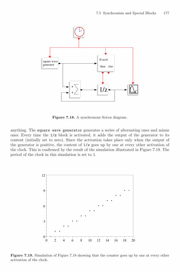
7.5 Synchronism and Special Blocks 177
then else
If in>0
then else
If in>0
generatorsquare wavegeneratorsquare wave
1/z1/z+
+
+
+
Figure 7.18. A synchronous Scicos diagram.
anything. The square wave generator generates a series of alternating ones and minusones. Every time the 1/z block is activated, it adds the output of the generator to itscontent (initially set to zero). Since the activation takes place only when the output ofthe generator is positive, the content of 1/z goes up by one at every other activation ofthe clock. This is confirmed by the result of the simulation illustrated in Figure 7.19. Theperiod of the clock in this simulation is set to 1.
0 2 4 6 8 10 12 14 16 18 200
3
6
9
12
+♦ ♦♦
♦♦ ♦♦
♦♦ ♦♦
♦♦ ♦♦
♦♦ ♦♦
♦♦ ♦♦
♦♦ ♦♦
♦♦ ♦♦
♦♦ ♦♦
♦♦ ♦
Figure 7.19. Simulation of Figure 7.18 showing that the counter goes up by one at every otheractivation of the clock.
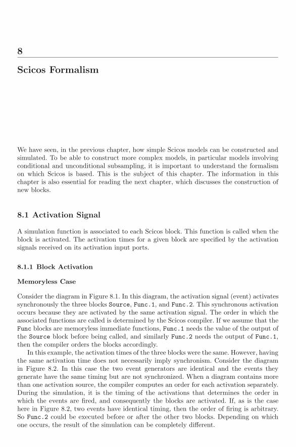
8
Scicos Formalism
We have seen, in the previous chapter, how simple Scicos models can be constructed andsimulated. To be able to construct more complex models, in particular models involvingconditional and unconditional subsampling, it is important to understand the formalismon which Scicos is based. This is the subject of this chapter. The information in thischapter is also essential for reading the next chapter, which discusses the construction ofnew blocks.
8.1 Activation Signal
A simulation function is associated to each Scicos block. This function is called when theblock is activated. The activation times for a given block are specified by the activationsignals received on its activation input ports.
8.1.1 Block Activation
Memoryless Case
Consider the diagram in Figure 8.1. In this diagram, the activation signal (event) activatessynchronously the three blocks Source, Func.1, and Func.2. This synchronous activationoccurs because they are activated by the same activation signal. The order in which theassociated functions are called is determined by the Scicos compiler. If we assume that theFunc blocks are memoryless immediate functions, Func.1 needs the value of the output ofthe Source block before being called, and similarly Func.2 needs the output of Func.1,then the compiler orders the blocks accordingly.
In this example, the activation times of the three blocks were the same. However, havingthe same activation time does not necessarily imply synchronism. Consider the diagramin Figure 8.2. In this case the two event generators are identical and the events theygenerate have the same timing but are not synchronized. When a diagram contains morethan one activation source, the compiler computes an order for each activation separately.During the simulation, it is the timing of the activations that determines the order inwhich the events are fired, and consequently the blocks are activated. If, as is the casehere in Figure 8.2, two events have identical timing, then the order of firing is arbitrary.So Func.2 could be executed before or after the other two blocks. Depending on whichone occurs, the result of the simulation can be completely different.
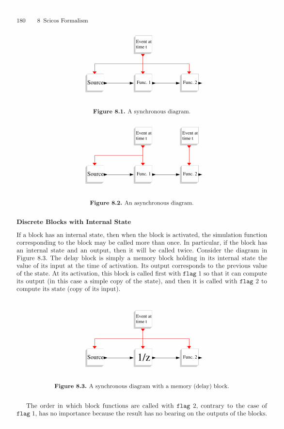
180 8 Scicos Formalism
SourceSource Func. 1Func. 1
time tEvent attime tEvent at
Func. 2Func. 2
Figure 8.1. A synchronous diagram.
SourceSource Func. 1Func. 1
time tEvent attime tEvent at
Func. 2Func. 2
time tEvent attime tEvent at
Figure 8.2. An asynchronous diagram.
Discrete Blocks with Internal State
If a block has an internal state, then when the block is activated, the simulation functioncorresponding to the block may be called more than once. In particular, if the block hasan internal state and an output, then it will be called twice. Consider the diagram inFigure 8.3. The delay block is simply a memory block holding in its internal state thevalue of its input at the time of activation. Its output corresponds to the previous valueof the state. At its activation, this block is called first with flag 1 so that it can computeits output (in this case a simple copy of the state), and then it is called with flag 2 tocompute its state (copy of its input).
SourceSource 1/z1/z
time tEvent attime tEvent at
Func. 2Func. 2
Figure 8.3. A synchronous diagram with a memory (delay) block.
The order in which block functions are called with flag 2, contrary to the case offlag 1, has no importance because the result has no bearing on the outputs of the blocks.
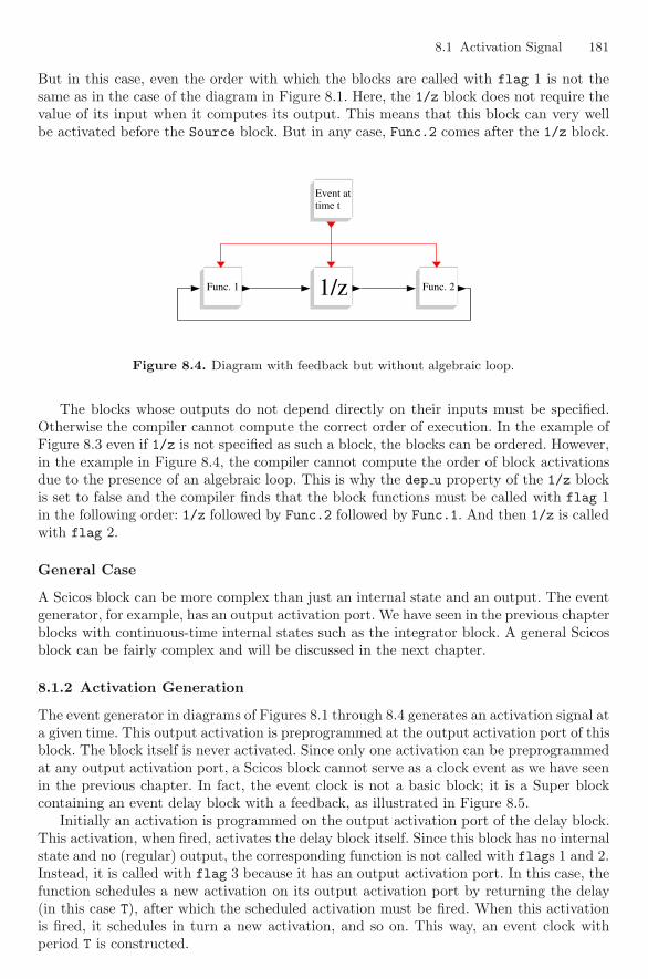
8.1 Activation Signal 181
But in this case, even the order with which the blocks are called with flag 1 is not thesame as in the case of the diagram in Figure 8.1. Here, the 1/z block does not require thevalue of its input when it computes its output. This means that this block can very wellbe activated before the Source block. But in any case, Func.2 comes after the 1/z block.
Func. 1Func. 1 1/z1/z
time tEvent attime tEvent at
Func. 2Func. 2
Figure 8.4. Diagram with feedback but without algebraic loop.
The blocks whose outputs do not depend directly on their inputs must be specified.Otherwise the compiler cannot compute the correct order of execution. In the example ofFigure 8.3 even if 1/z is not specified as such a block, the blocks can be ordered. However,in the example in Figure 8.4, the compiler cannot compute the order of block activationsdue to the presence of an algebraic loop. This is why the dep u property of the 1/z blockis set to false and the compiler finds that the block functions must be called with flag 1in the following order: 1/z followed by Func.2 followed by Func.1. And then 1/z is calledwith flag 2.
General Case
A Scicos block can be more complex than just an internal state and an output. The eventgenerator, for example, has an output activation port. We have seen in the previous chapterblocks with continuous-time internal states such as the integrator block. A general Scicosblock can be fairly complex and will be discussed in the next chapter.
8.1.2 Activation Generation
The event generator in diagrams of Figures 8.1 through 8.4 generates an activation signal ata given time. This output activation is preprogrammed at the output activation port of thisblock. The block itself is never activated. Since only one activation can be preprogrammedat any output activation port, a Scicos block cannot serve as a clock event as we have seenin the previous chapter. In fact, the event clock is not a basic block; it is a Super blockcontaining an event delay block with a feedback, as illustrated in Figure 8.5.
Initially an activation is programmed on the output activation port of the delay block.This activation, when fired, activates the delay block itself. Since this block has no internalstate and no (regular) output, the corresponding function is not called with flags 1 and 2.Instead, it is called with flag 3 because it has an output activation port. In this case, thefunction schedules a new activation on its output activation port by returning the delay(in this case T), after which the scheduled activation must be fired. When this activationis fired, it schedules in turn a new activation, and so on. This way, an event clock withperiod T is constructed.

182 8 Scicos Formalism
TDelay TDelay
11
Figure 8.5. An event clock.
8.2 Inheritance
In the examples of the previous chapter, we had encountered many blocks without activa-tion input ports. Consider the diagram in Figure 8.6. Normally the Func.1 block shouldnot be activated because it receives no activation signal. But by convention, in the absenceof input activation ports, a block inherits its activation from its regular input.
SourceSource Func. 1Func. 1
time tEvent attime tEvent at
Figure 8.6. The block Func.1 is activated by inheritance.
The inheritance mechanism is implemented at a precompilation phase. For example,in the case of the diagram in Figure 8.6, the precompiler adds the missing activation portand link as illustrated in Figure 8.7. The user never sees this diagram; the precompilationphase is completely transparent to the user.
If the block has more than one regular input, the inheritance mechanism places asmany activation input ports on the block as the block has regular input ports. See thediagram in Figure 8.8 and the diagram obtained after the precompilation phase illustratedin Figure 8.9. The + block outputs an activation signal with activation times correspondingto the union of input activation times.
We see here that a block can have more than one activation input port. In this case,the block is activated when it receives an event on one or the other of its input activationports. Thus the block is activated at the union of the two activation times. This explainshow Func.2 inherits its activation.
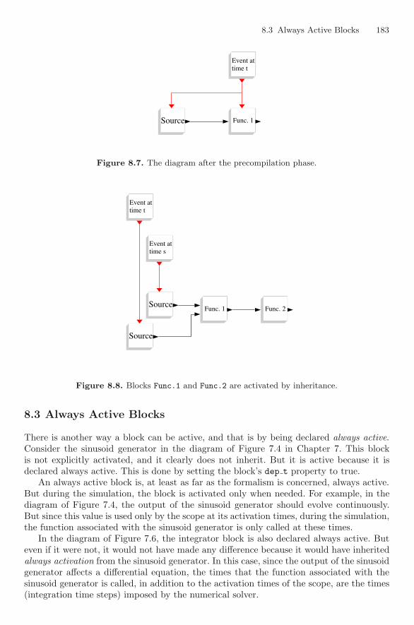
8.3 Always Active Blocks 183
SourceSource Func. 1Func. 1
time tEvent attime tEvent at
Figure 8.7. The diagram after the precompilation phase.
SourceSourceFunc. 1Func. 1
time tEvent attime tEvent at
time sEvent attime sEvent at
SourceSource
Func. 2Func. 2
Figure 8.8. Blocks Func.1 and Func.2 are activated by inheritance.
8.3 Always Active Blocks
There is another way a block can be active, and that is by being declared always active.Consider the sinusoid generator in the diagram of Figure 7.4 in Chapter 7. This blockis not explicitly activated, and it clearly does not inherit. But it is active because it isdeclared always active. This is done by setting the block’s dep t property to true.
An always active block is, at least as far as the formalism is concerned, always active.But during the simulation, the block is activated only when needed. For example, in thediagram of Figure 7.4, the output of the sinusoid generator should evolve continuously.But since this value is used only by the scope at its activation times, during the simulation,the function associated with the sinusoid generator is only called at these times.
In the diagram of Figure 7.6, the integrator block is also declared always active. Buteven if it were not, it would not have made any difference because it would have inheritedalways activation from the sinusoid generator. In this case, since the output of the sinusoidgenerator affects a differential equation, the times that the function associated with thesinusoid generator is called, in addition to the activation times of the scope, are the times(integration time steps) imposed by the numerical solver.

184 8 Scicos Formalism
SourceSourceFunc. 1Func. 1
time tEvent attime tEvent at
time sEvent attime sEvent at
SourceSource
Func. 2Func. 2
Figure 8.9. The diagram after the precompilation phase.
8.4 Constant Blocks
A block without input, not explicitly activated and not being always active, is a constantblock. A constant block’s outputs do not evolve as a function of time. During the sim-ulation, the function associated with a constant block is called only at the initializationphase. The same holds for blocks inheriting from constant blocks. See, for example, thediagram in Figure 8.10. If Source is not always active, then it is a constant. If Func.1 isnot always active, it inherits its activation, or more specifically its absence of activation,from the Source block. The Func.1 block’s function is called just once to compute itsoutput after the initialization phase. This is, of course, reasonable because the output ofFunc.1 does not evolve.
SourceSource Func. 1Func. 1
Figure 8.10. Inheritance from a constant block.
8.5 Conditional Blocks
In many applications, in particular in signal processing, signals with different frequenciesinteract in the same model. A common situation is the decimation operation, which consistsin generating a signal B from a signal A by taking one out of every n values of A. Thefrequency of signal B is then that of signal A divided by n. To implement this operation,one might consider using two independent clocks to fix the two frequencies. This is donein the diagram of Figure 8.11 using a sample and hold block.
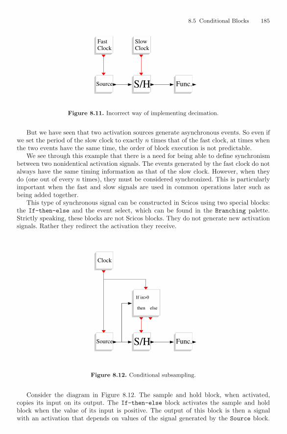
8.5 Conditional Blocks 185
SourceSource S/HS/H
ClockSlowClockSlow
ClockFastClockFast
Func.Func.
Figure 8.11. Incorrect way of implementing decimation.
But we have seen that two activation sources generate asynchronous events. So even ifwe set the period of the slow clock to exactly n times that of the fast clock, at times whenthe two events have the same time, the order of block execution is not predictable.
We see through this example that there is a need for being able to define synchronismbetween two nonidentical activation signals. The events generated by the fast clock do notalways have the same timing information as that of the slow clock. However, when theydo (one out of every n times), they must be considered synchronized. This is particularlyimportant when the fast and slow signals are used in common operations later such asbeing added together.
This type of synchronous signal can be constructed in Scicos using two special blocks:the If-then-else and the event select, which can be found in the Branching palette.Strictly speaking, these blocks are not Scicos blocks. They do not generate new activationsignals. Rather they redirect the activation they receive.
SourceSource S/HS/H
ClockClock
Func.Func.
then else
If in>0
then else
If in>0
Figure 8.12. Conditional subsampling.
Consider the diagram in Figure 8.12. The sample and hold block, when activated,copies its input on its output. The If-then-else block activates the sample and holdblock when the value of its input is positive. The output of this block is then a signalwith an activation that depends on values of the signal generated by the Source block.
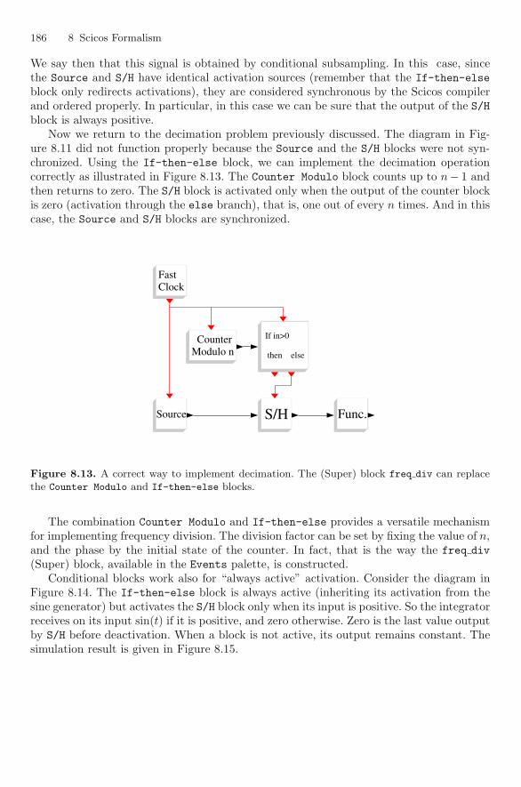
186 8 Scicos Formalism
We say then that this signal is obtained by conditional subsampling. In this case, sincethe Source and S/H have identical activation sources (remember that the If-then-elseblock only redirects activations), they are considered synchronous by the Scicos compilerand ordered properly. In particular, in this case we can be sure that the output of the S/Hblock is always positive.
Now we return to the decimation problem previously discussed. The diagram in Fig-ure 8.11 did not function properly because the Source and the S/H blocks were not syn-chronized. Using the If-then-else block, we can implement the decimation operationcorrectly as illustrated in Figure 8.13. The Counter Modulo block counts up to n− 1 andthen returns to zero. The S/H block is activated only when the output of the counter blockis zero (activation through the else branch), that is, one out of every n times. And in thiscase, the Source and S/H blocks are synchronized.
SourceSource S/HS/H
ClockFastClockFast
Func.Func.
then else
If in>0
then else
If in>0
Modulo n CounterModulo n Counter
Figure 8.13. A correct way to implement decimation. The (Super) block freq div can replacethe Counter Modulo and If-then-else blocks.
The combination Counter Modulo and If-then-else provides a versatile mechanismfor implementing frequency division. The division factor can be set by fixing the value of n,and the phase by the initial state of the counter. In fact, that is the way the freq div(Super) block, available in the Events palette, is constructed.
Conditional blocks work also for “always active” activation. Consider the diagram inFigure 8.14. The If-then-else block is always active (inheriting its activation from thesine generator) but activates the S/H block only when its input is positive. So the integratorreceives on its input sin(t) if it is positive, and zero otherwise. Zero is the last value outputby S/H before deactivation. When a block is not active, its output remains constant. Thesimulation result is given in Figure 8.15.
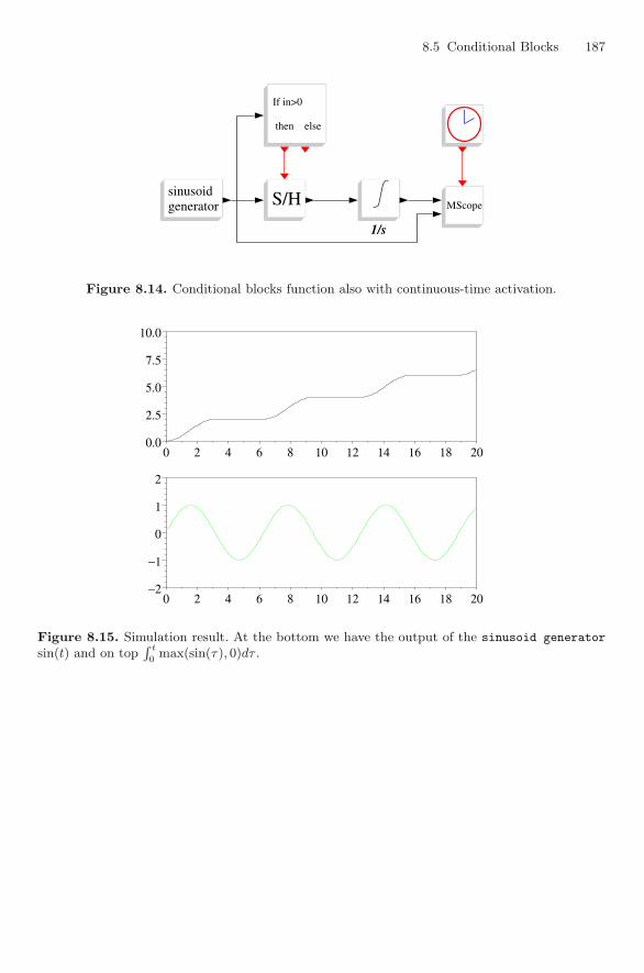
8.5 Conditional Blocks 187
S/HS/H
1/s
then else
If in>0
then else
If in>0
generatorsinusoidgeneratorsinusoid
MScopeMScope
Figure 8.14. Conditional blocks function also with continuous-time activation.
0 2 4 6 8 10 12 14 16 18 200.0
2.5
5.0
7.5
10.0
+
0 2 4 6 8 10 12 14 16 18 20−2
−1
0
1
2
+
Figure 8.15. Simulation result. At the bottom we have the output of the sinusoid generator
sin(t) and on topR t
0max(sin(τ), 0)dτ .

9
Scicos Blocks
A block is a basic module from which Scicos diagrams are constructed. A block correspondsto an operation, and by interconnecting blocks through links, we construct (implement) analgorithm. So in a sense, blocks in Scicos are the counterpart of functions in a programminglanguage, and as in programming languages, some blocks are provided through standardlibraries, while others are developed by the user.
Most Scicos users never need to develop a new block because standard libraries con-tain a large number of blocks providing most of the elementary functionalities needed inthe construction of Scicos diagrams; moreover, blocks such as Mathematical Expressionallow the user to define block functionality in terms of Scilab expressions without loss ofefficiency (the Scilab expression in this case is compiled). That is why readers can skipthis chapter on a first reading and come back to it when they want to learn about blockconstruction.
9.1 Block Behavior
A Scicos block can be a complex entity. It can have multiple vector inputs and outputs, acontinuous-time vector state, a discrete-time vector state, zero-crossing surfaces, etc., asshown in Figure 9.1. But most Scicos blocks do not contain all of these features simulta-neously.
The behavior of a block is primarily specified by the way it is activated. We have seenin the previous section that a block is activated in three different ways. The way the blocklearns about the way it is activated is via an activation index nevprt.
9.1.1 External Activation
A block is activated when it receives activations on its activation input ports. As we haveseen in the previous section, such activations can also be inherited when the block has noactivation input ports, in which case the corresponding activation ports are added by theScicos compiler and the activations are considered to be external.
In the case of external activation, the activation index nevprt is a positive integerobtained by the following formula:
nevprt =n∑
j=1
ij2j−1, (9.1)
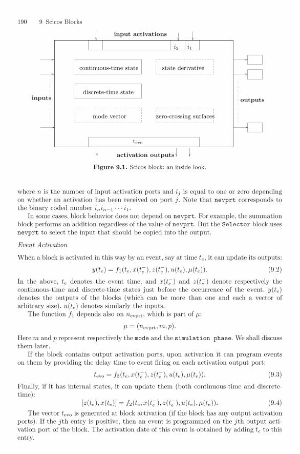
190 9 Scicos Blocks
continuous-time state
discrete-time state
mode vector zero-crossing surfaces
state derivative
inputs outputs
i1i2
tevo
input activations
activation outputs
Figure 9.1. Scicos block: an inside look.
where n is the number of input activation ports and ij is equal to one or zero dependingon whether an activation has been received on port j. Note that nevprt corresponds tothe binary coded number inin−1 · · · i1.
In some cases, block behavior does not depend on nevprt. For example, the summationblock performs an addition regardless of the value of nevprt. But the Selector block usesnevprt to select the input that should be copied into the output.
Event Activation
When a block is activated in this way by an event, say at time te, it can update its outputs:
y(te) = f1(te, x(t−e ), z(t−e ), u(te), μ(te)). (9.2)
In the above, te denotes the event time, and x(t−e ) and z(t−e ) denote respectively thecontinuous-time and discrete-time states just before the occurrence of the event. y(te)denotes the outputs of the blocks (which can be more than one and each a vector ofarbitrary size). u(te) denotes similarly the inputs.
The function f1 depends also on nevprt, which is part of μ:
μ = (nevprt, m, p).
Here m and p represent respectively the mode and the simulation phase. We shall discussthem later.
If the block contains output activation ports, upon activation it can program eventson them by providing the delay time to event firing on each activation output port:
tevo = f3(te, x(t−e ), z(t−e ), u(te), μ(te)). (9.3)
Finally, if it has internal states, it can update them (both continuous-time and discrete-time):
[z(te), x(te)] = f2(te, x(t−e ), z(t−e ), u(te), μ(te)). (9.4)
The vector tevo is generated at block activation (if the block has any output activationports). If the jth entry is positive, then an event is programmed on the jth output acti-vation port of the block. The activation date of this event is obtained by adding te to thisentry.
9.1 Block Behavior 191
Continuous-Time Activation
If a source of block activation is “always activation,” then activation occurs over timeintervals and not at specific times as in the case of event activation. See, for example, thediagram in Figure 8.14. In this case, the output calculation given in equation (9.2), thanksto the continuity assumption of all the signals over a continuous-time activation period,can be simplified as follows:
y(t) = f1(t, x(t), z(t), u(t), μ(t)). (9.5)
The output activation programming and state updates do not apply in this case, but ifthe block has a continuous-time state, it evolves according to the following differentialequation,
x = f0(t, x(t), z(t), u(t), μ(t)) (9.6)
over the activation period, which we call the simulation phase 2, as opposed to eventactivation instances which are referred to as simulation phase 1 . Note that z(t), likenevprt, is constant over this period. So is the mode m if there is one.
Mode and Zero-Crossing
The mode parameter is not part of the Scicos formalism. It is introduced to facilitate theimplementation of the numerical solver. Most blocks that a user may have to constructdon’t need any mode or zero-crossing, and the user can use existing blocks with modeand zero-crossing without a complete understanding of the way they work. For the sakeof completeness, however, we give a short presentation below. More details can be foundin the examples provided later in this chapter.
Numerical integrators can experience step size control and other problems at placeswhere the functions being integrated are not continuously differentiable. If f1 or f0 is notsmooth (continuously differentiable) at some points, then mode is used in such a way asto make sure the numerical solver never encounters these points of discontinuity inside anintegration interval.
Consider the following simple example: y = u if u ≥ 0, and y = −u otherwise. Thisfunction realizes the absolute-value function and is not differentiable at 0. In this case, amode can be defined to specify at the start of the integration period whether u is positive.To make sure the integration stops when the sign of u changes, a zero-crossing surface isintroduced at zero. During the integration period (which could end because of the zero-crossing), the output y is computed as follows: y = u if m = 1, and y = −u otherwise. Afterthe zero-crossing the mode is recomputed and the integration continues. The computationof the mode and the zero-crossing surface are performed by the block. If the simulationphase is 1, we have
[m(t), s(t)] = f9(t, x(t), z(t), u(t), μ(t)). (9.7)
The zero-crossing surfaces s(t) may be present even if the block has no mode. When azero-crossing occurs, the block is internally activated, which means that (9.3) and (9.4)are called with nevprt = −1. The blocks in the Threshold palette, for example, havezero-crossings but no modes.
9.1.2 Always Activation
A block can be declared always active. This is, for example, the case of the sine generatorblock. In this case the nevprt index is zero. Always activation can be thought of as

192 9 Scicos Blocks
an activation received on a fictitious activation input port 0 that would correspond tonevprt = 0.
Always activation is a special case of continuous-time activation where the activationperiod is equal to the period of simulation. So the behavior of the block is specified againby equations (9.5) and (9.6) with nevprt set to zero.
9.1.3 Internal Zero-Crossing
When a zero-crossing occurs inside a block, this block is activated with nevprt equal to −1at the time of crossing. If this time is denoted by te, then the state update formula isgiven by (9.4) with nevprt = −1. This type of activation is used, for example, in thebouncing balls demo block of Scicos to change the direction of balls (characterized by thecontinuous-time state of the block) after a collision.
9.2 Blocks Inside Palettes
Scicos libraries of blocks are called palettes. There are a number of standard palettesavailable in Scicos providing many elementary blocks.
The available palettes are the following:
• Sources library. It includes signal generators such as the square-wave, sawtooth, andsine-wave generators, and also read from file blocks. The read from file blocks generatesignals from data stored on files.
• Sinks library. It includes blocks that store signals on a file or display signals on ascreen. These blocks have no output ports.
• Branching library. This palette contains switches, multiplexers, selectors, and arelay. It also includes two very special blocks that redirect activation signals: theIf-then-else and the events select blocks.
• Non linear library. The blocks in this palette realize memoryless nonlinear operatorssuch as trigonometric functions, multiplication, logarithm, inversion, and saturation.The palette also includes interpolation and table lookup blocks, and a special blockcalled Mathematical Expression used to express a nonlinear operator in terms of aScilab expression. The constraint on the scilab expressions is that only scalar expres-sions can be used, but the evaluation is very efficient.
• Events library. This library includes blocks for generating and manipulating events(activation signals). It also includes the block Stop, which halts the simulation if acti-vated.
• Threshold library. The blocks included in this palette can generate events when asignal crosses zero.
• Others library. This palette includes a number of blocks useful for the constructionof new blocks: Cblock2, Scifunc, GENERIC,. . . . These blocks are discussed later in thischapter. It also includes logical and relational blocks. It also includes the Text block,which is not a real block, but a way to place text inside a diagram.
• Linear library. This palette contains blocks realizing linear operators such as summa-tion, gain, and many dynamical linear systems in both continuous and discrete time.Delay blocks and jump linear systems are also included in this palette.
The above palettes provide general-purpose blocks. Specialized palettes can be addedby the user. Two such palettes are included. One is an electrical palette. The other isa Thermo-Hydraulic palette.

9.4 Super Block and Scifunc 193
9.3 Modifying Block Parameters
Most blocks have parameters that must be changed by the user for specific applications.Block parameters can be changed by “opening” a block (clicking at the center of theblock). This action opens a dialog box, which can be used to define new parameter values.
Blocks parameters are stored in two different ways:
1. Symbolically: the exact expression entered for each parameter in the dialog box isstored as Scilab text. For example, the user can enter 2*%pi, and this expression issaved and shown the next time the dialog box is opened.
2. Numerically: the expression is evaluated and the numerical value is saved.
It may seem redundant to store parameter values in two different ways but there aregood reasons for doing this. One reason is that it is more convenient to see 2*%pi the nexttime the dialog box is opened than it is to see 6.2831853. But the main reason is thatthe values of the parameters can be defined in terms of Scilab variables already definedin the context of the diagram. For example, a parameter can be set to sin(x)*y. Thenumerical value of this parameter is evaluated based on the values of x and y defined inthe context of the diagram. Keeping the symbolic expression allows Scicos to update thevalue of the parameter when x or y is modified in the context. In this case, x and y aresymbolic parameters.
9.4 Super Block and Scifunc
In addition to the blocks available in Scicos palettes, the user can create and use customblocks by adapting existing blocks. There are various ways of doing this.
• using the Super block facility,• using Scifunc blocks, which allow block functionality to be defined on-line by Scilab
expressions.• using C or Scilab programs, dynamically linked with, or loaded in, Scilab.
The third method, which will be presented in the next section, gives the best resultsas far as simulation performance is concerned, provided a C program is used.
9.4.1 Super Blocks
To construct a Super block, the user should copy the “Super block” block from the Otherspalette into the Scicos window and click on it. This will open up a new Scicos windowin which the Super block should be defined. Super blocks can also be defined using theRegion-to-Super-block facility, which creates a Super block from existing blocks in aspecified region of the diagram.
The construction of the Super block model is done in the same way as the earlierdiagrams, that is, by copying and pasting blocks from various palettes into the Superblock’s editor window and connecting them. Input and output ports of the Super blockshould be specified by input and output block ports available in the Sources and Sinkspalettes. Super blocks can, of course, be used within Super blocks.
A Super block can be saved in various formats. If the Super block is of interest in otherconstructions, it can be converted into a block and placed in a user palette. This can bedone in various ways:
194 9 Scicos Blocks
• The Save-as-Interf-Func facility can save the Super block in two different ways:as a block or as a Super block. The difference is that in the block case, the contentof the Super block is no longer visible, whereas in the Super block case, the savedSuper block would have exactly the same behavior as the Super block being saved.Save-as-Interf-Func should be used inside the Super block of interest.By default, in the block case, the dialog menus of the new block are generated auto-matically using the dialog menus of all the blocks within the Super block. This is oftencumbersome, and most users need to edit the new interfacing function. This Scilabfunction is easily customizable.Once the Super block, or more specifically the corresponding Scilab interfacing func-tion, is saved, either as a block or as a Super block, it can be used in Scicos. This canbe done using Add-new-block in the Edit menu. The block can also be placed in apalette for future use. See Section 9.6.
• Using Code-Generation. Under certain conditions, the dynamics of the content of aSuper block can be expressed using a single C program. Code-Generation generatesthis program automatically; see Section 12.
If the Super block is used only in a particular construction for one Scicos diagram, thenthe Super block need not be saved. A click on the Exit will close the Super block windowand activate the main Scicos window (or another Super block window if the Super blockwas being defined within another Super block). Saving the block diagram automaticallysaves the content of all Super blocks used inside of it.
A Super block, like any other block, can be duplicated using the Copy button. In thatcase all the contents of the Super block are duplicated.
9.4.2 Scifunc
The Scifunc block enables using the Scilab language for defining, on-line, new Scicosblocks. Block information, such as the number of inputs and outputs, initial states, theinitial firing vector, and information regarding the behavior of the block during simulationhave to be entered by the user. This input consists essentially of Scilab expressions definingfunctions fi (presented in Section 9.1). This is done interactively by clicking on the Scifuncblock once it is copied into the Scicos window. The main disadvantage of Scifunc isthat the dialog for updating block parameters cannot be customized. In order to have acustomized dialog box, a Scilab function called the interfacing function must be developed.We shall see how this is done in Section 9.5.1.
It should be noted that in the case of Scifunc, like all older types of Scicos blocks, thefunction f3 must return the time of the outgoing events and not the delay with respect tothe activation time of the block.
9.5 Constructing New Basic Blocks
In this section we show how a new basic block can be constructed and used in Scicos.Each Scicos basic block is defined by two functions. The first one, which must be in the
Scilab language, handles the interactions with the editor. It is this function that specifieswhat the geometry of the block should be, how many inputs and outputs it should have,what the block type is, etc. It is also this function that handles the user interface (updatingblock parameters and initializing the states). This function is referred to as the interfacingfunction.
9.5 Constructing New Basic Blocks 195
The second function, which is called the computational function, is normally writtenin C, but can also be a Scilab function. This function defines the behavior of the blockduring the simulation. For simple blocks, this amounts to coding the fi functions whichhave to be evaluated by the program depending on the value of an input flag. The i in fi
corresponds to the value of the flag. We shall come back to this in Section 9.5.2. In order toget the best performance, this part of the Scicos block should be defined by C programs,but Scilab functions are often used in the early phases of development for testing anddebugging purposes since they are easier to write.
Even though each basic block requires both an interfacing function and a computationalfunction, the user often needs to be developed only one. For example, a computationalfunction can be used with the GENERIC block available in the Others palette. The GENERICblock is a generic interfacing function. It suffices to specify the “name of the computationalfunction” in the dialog box of the GENERIC block along with information concerning theinput/output numbers and sizes, initial states, etc. The name of the program, in the caseof C programs, is the name of the entry point when the C program is incrementally linkedwith Scilab (see Section 9.5.2). In the case of a Scilab program, it is simply the name ofthe Scilab function. Scilab functions must, of course, be loaded as usual into Scilab beforeScicos is launched. This can be done using either getf or load if the function is containedin a library. See Section 2.5.
The drawback of using the GENERIC block, as in the case of Scifunc, is the generic dia-log box. In most cases, it is desirable to customize both the block’s dialog box and its look.For that, a custom interfacing function must be used. This Scilab function should provideinformation on the geometry of the block and handle the dialog for defining and updatingblock parameters and states. The interfacing function is used by the graphical editor,as opposed to the computational function, which is used by the simulator. Section 9.5.1describes how the interfacing function and the underlying programs should be developed.
On the other hand, in some cases a new block may consist simply of a new inter-facing function using an existing computational function. Consider, for example, the twocontinuous-time linear dynamical system blocks in the Linear palette. One is in state-spaceform and the dialog requests the A, B, C, D matrices. The other uses transfer functionsand the user should enter the transfer function of the system. But both of these blocks usethe same computational function, namely csslti. The reason is that the transfer functionis converted to a state-space representation in the corresponding interfacing function. Sotwo blocks may look very different but have a common computational function.
A new block realizing a low-pass filter should have a dialog where information such asthe cut-off frequency, order, overshoot, etc., are specified. But once the filter is designed inthe interfacing function (using specialized Scilab functions), the simulation can very wellbe performed with csslti. The reason is that the filter is nothing but a linear systemcharacterized by A, B, C, D matrices.
9.5.1 Interfacing Function
The interfacing function is used only by the Scicos editor. In particular, it is used to ini-tialize, draw, connect the block, and to modify its parameters. In addition, the interfacingfunction initializes block states and specifies certain block properties. It also specifies thename of the computational function to be used by the simulator. What the interfacingfunction should return depends on an input flag job.
Syntax
[x,y,typ]=block(job,arg1,arg2)
196 9 Scicos Blocks
Parameter job
The parameter job can take on the following values:
• ’plot’: the function draws the block and its label. arg1 is the data structure of theblock. arg2,x,y,typ are unused.In general, the standard draw function can be used. It draws a rectangular block.
• ’getinputs’: the function returns the position and type of input ports (regular andevent). arg1 is the data structure of the block. arg2 is unused. x is the vector of xcoordinates of input ports. y is the vector of y coordinates of input ports. typ is thevector of input ports types.In general, the standard input function can be used.
• ’getoutputs’: returns position and type of output ports (regular and event). arg1 is thedata structure of the block. arg2 is unused. x is the vector of x coordinates of outputports. y is the vector of y coordinates of output ports. typ is the vector of output portstypes .In general, the standard output function can be used. The standard input andstandard output functions place regular input/outputs on the side of the block andthe activation inputs on top and activation outputs at the bottom of the block.
• ’getorigin’: returns coordinates of the lower left point of the rectangle containing theblock’s shape. arg1 is the data structure of the block. arg2 is unused. x is the vectorof x coordinates of output ports. y is the vector of y coordinates of output ports. typis unused.In general, the standard origin function can be used.
• ’set’: This function opens a dialog for block parameter acquisition. arg1 is the datastructure of the block. arg2 is unused. x is the new data structure of the block. y isunused. typ is unused.
• ’define’: provides initialization of the block’s data structure. It sets block’s initial type,number of inputs, number of outputs, etc. arg1, arg2 are unused. x is the data struc-ture of the block. y is unused. typ is unused.
Example: the Interfacing Function of the Absolute Value Block
function [x,y,typ]=ABS_VALUE(job,arg1,arg2)
x=[];y=[];typ=[]
select job
case ’plot’ thenstandard_draw(arg1)
case ’getinputs’ then[x,y,typ]=standard_inputs(arg1)
case ’getoutputs’ then[x,y,typ]=standard_outputs(arg1)
case ’getorigin’ then[x,y]=standard_origin(arg1)
case ’set’ thenx=arg1;
graphics=arg1.graphics;exprs=graphics.exprs
model=arg1.model;
while %t do
[ok,zcr,exprs]=..
getvalue(’Set block parameters’,..
9.5 Constructing New Basic Blocks 197
[’use zero_crossing (1: yes) (0:no)’],..
list(’vec’,1),exprs)
if ~ok then break, endgraphics.exprs=exprs
if ok thenif zcr<>0 thenmodel.nmode=-1;model.nzcross=-1;
elsemodel.nmode=0;model.nzcross=0;
endx.graphics=graphics;x.model=model
breakend
endcase ’define’ thennu=-1
model=scicos_model()
model.sim=list(’absolute_value’,4)
model.in=nu
model.out=nu
model.nzcross=nu
model.nmode=nu
model.blocktype=’c’
model.dep_ut=[%t %f]
exprs=[string([1])]
gr_i=[’txt=[’’ABS’’];’;
’xstringb(orig(1),orig(2),txt,sz(1),sz(2),’’fill’’)’]
x=standard_define([2 2],model,exprs,gr_i)
endendfunction
The data structures used in the interfacing function are explained in Appendix A.The only hard part of defining an interfacing function is in the ’set’ case. Note thatthe function getvalue is used to create a dialog for the block. This should be done in alluser-defined blocks as well, since this function is overloaded, when Eval is performed, toread and evaluate block parameters. getvalue is a generic dialog box with built-in typechecking facilitating the implementation of Scicos blocks’ dialog boxes.
9.5.2 Computational Function
The computational function is called in various ways by the simulator. The way the blockis called (the calling sequence) is characterized by the type of the interfacing function. It isstrongly recommended that type 4 and 5 computational functions now be used. The othertypes are now obsolete. Type 4 is used for programs written in C and type 5 for Scilabcomputational functions.
Type 4 C functions receive two arguments: a structure containing block informationand a flag:
#include "scicos_block.h"
#include <math.h>
void my block(scicos block *block,int flag)

198 9 Scicos Blocks
{. . .
}
flag
The flag indicates the job that the computational function must perform. It usually consistsin updating some of the fields of the block structure. Specifically, the following jobs exist:
• Initialization: If the function is called with flag=4, then the continuous and discretestates can be initialized, or more specifically, reinitialized (if necessary) because they arealready initialized by the interfacing function. The block output can also be initialized.This option is not used in most blocks. It is used by the ones that read and writedata from files, for opening the file, or by scope for initializing the graphics window.It is also used by blocks, which require dynamically allocated memory; the allocationis done under this flag. Each block is called once and only once at the beginning of thesimulation with flag 4.
• Output update: When flag=1, the simulator is requesting the outputs of the block.The computational function should use the needed information within the block’s struc-ture (inputs, states, nevprt, which codes the way by which the activation has arrived,etc.) to compute the outputs and place them at the addresses given in the block struc-ture. Note that if the block contains different modes, then the way the output iscomputed depends on the simulation phase. The simulation phase indicates whetherthe call is made in the numerical integration phase or is due to an event.
• State update: When the simulator calls the function with flag=2, it means that anevent has activated the block (nevprt�= 0). The activation may also be due to aninternal zero-crossing event, in which case nevprt is equal to −1. With flag= 2, thesimulator is asking the block to update its states x and z. Scicos provides the addressesof the states, where old values of x and z reside, and the block should update themin place. This avoids useless and time-consuming copies, in particular when part orall of x or z is not to be changed. If a temporary workspace is needed to performthe computations, it can either be statically allocated in the C routine or dynamicallyallocated when the block is called with flag 4.If nevprt= −1, indicating that the activation is due to an internal zero-crossing, thenthe vector jroot specifies which surfaces have been crossed and in which direction. Inparticular, if the ith entry of jroot is 0, then the ith surface (counting from zero) hasnot crossed zero. If it is +1 (respectively −1), then it has crossed zero with a positive(respectively negative) slope.
• Integrator calls: During the integration, the solver calls the function for the value ofx. This is done with flag=0. The computational function must compute x and place itin the address provided in the block structure.
• Mode and zero-crossing: Scicos solvers assume model smoothness. This means thatthe behavior of blocks, which contain or affect continuous-time states of the systemmust be smooth, or at least piecewise smooth. In this latter case, the points of nons-moothness must be specified in such a way that the solver can, if needed, issue a coldrestart when going through such points. An example of such a block is the ABS block.The absolute value function is smooth except at zero, where it is not even differen-tiable. In this case, we say that the absolute value block has two modes: one where theoutput equals the input, and one where the output is the negative of the input. A blockmay have many different modes, which are stored in the block structure. The point of
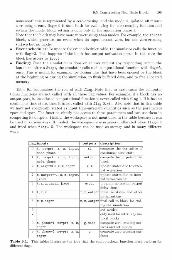
9.5 Constructing New Basic Blocks 199
nonsmoothness is represented by a zero-crossing, and the mode is updated after sucha crossing occurs. flag= 9 is used both for evaluating the zero-crossing function andsetting the mode. Mode setting is done only in the simulation phase 1.Note that the block may have more zero-crossings than modes. For example, the zcrossblock, which generates an event when its input crosses zero, has one zero-crossingsurface but no mode.
• Event scheduler: To update the event scheduler table, the simulator calls the functionwith flag=3. This happens if the block has output activation ports. In this case theblock has access to jroot.
• Ending: Once the simulation is done or at user request (by responding End in theRun menu after a Stop), the simulator calls each computational function with flag=5,once. This is useful, for example, for closing files that have been opened by the blockat the beginning or during the simulation, to flush buffered data, and to free allocatedmemory.
Table 9.1 summarizes the role of each flag. Note that in most cases the computa-tional functions are not called with all these flag values. For example, if a block has nooutput port, its associated computational function is never called with flag 1. If it has nocontinuous-time state, then it is not called with flag 0, etc. Also note that in this tablewe have not specifically stated as input time-invariant quantities such as the parametersrpar and ipar. The function clearly has access to these parameters and can use them incomputing its outputs. Finally, the workspace is not mentioned in the table because it canbe used in various ways. If needed, the workspace w is in general allocated when flag= 4and freed when flag= 5. The workspace can be used as storage and in many differentways.
flag inputs outputs description
0 t, nevprt, x, z, inptr,mode, phase
xd compute the derivative ofcontinuous time state
1 t, nevprt, x, z, inptr,mode, phase
outptr compute the outputs of theblock
2 t, nevprt>0, x, z, inptr x, z update states due to exter-nal activation
2 t, nevprt=-1, x, z, inptr,jroot
x, z update states due to inter-nal zero-crossing
3 t, x, z, inptr, jroot evout program activation outputdelay times
4 t, x, z x, z, outptr initialize states and otherinitializations
5 x, z, inptr x, z, outptr final call to block for end-ing the simulation
6 not needed
7 only used for internally im-plicit blocks
9 t, phase=1, nevprt, x, z,inptr
g, mode compute zero-crossing sur-faces and set modes
9 t, phase=2, nevprt, x, z,inptr
g compute zero-crossing sur-faces
Table 9.1. This tables illustrates the jobs that the computational function must perform fordifferent flags.
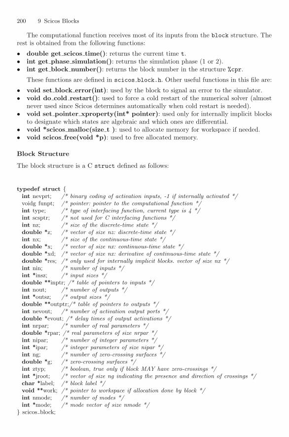
200 9 Scicos Blocks
The computational function receives most of its inputs from the block structure. Therest is obtained from the following functions:
• double get scicos time(): returns the current time t.• int get phase simulation(): returns the simulation phase (1 or 2).• int get block number(): returns the block number in the structure %cpr.
These functions are defined in scicos block.h. Other useful functions in this file are:
• void set block error(int): used by the block to signal an error to the simulator.• void do cold restart(): used to force a cold restart of the numerical solver (almost
never used since Scicos determines automatically when cold restart is needed).• void set pointer xproperty(int* pointer): used only for internally implicit blocks
to designate which states are algebraic and which ones are differential.• void *scicos malloc(size t ): used to allocate memory for workspace if needed.• void scicos free(void *p): used to free allocated memory.
Block Structure
The block structure is a C struct defined as follows:
typedef struct {int nevprt; /* binary coding of activation inputs, -1 if internally activated */voidg funpt; /* pointer: pointer to the computational function */int type; /* type of interfacing function, current type is 4 */int scsptr; /* not used for C interfacing functions */int nz; /* size of the discrete-time state */double *z; /* vector of size nz: discrete-time state */int nx; /* size of the continuous-time state */double *x; /* vector of size nx: continuous-time state */double *xd; /* vector of size nx: derivative of continuous-time state */double *res; /* only used for internally implicit blocks. vector of size nx */int nin; /* number of inputs */int *insz; /* input sizes */double **inptr; /* table of pointers to inputs */int nout; /* number of outputs */int *outsz; /* output sizes */double **outptr;/* table of pointers to outputs */int nevout; /* number of activation output ports */double *evout; /* delay times of output activations */int nrpar; /* number of real parameters */double *rpar; /* real parameters of size nrpar */int nipar; /* number of integer parameters */int *ipar; /* integer parameters of size nipar */int ng; /* number of zero-crossing surfaces */double *g; /* zero-crossing surfaces */int ztyp; /* boolean, true only if block MAY have zero-crossings */int *jroot; /* vector of size ng indicating the presence and direction of crossings */char *label; /* block label */void **work; /* pointer to workspace if allocation done by block */int nmode; /* number of modes */int *mode; /* mode vector of size nmode */
} scicos block;
9.5 Constructing New Basic Blocks 201
Examples
The simplest computational functions are those that simply compute an output as asmooth function of an input. One such function is the computational function of theSUMMATION block:
#include "scicos_block.h"
#include <math.h>
void summation(scicos block *block,int flag){
int j,k;if(flag==1){
if (block−>nin==1){block−>outptr[0][0]=0.0;for (j=0;j<block−>insz[0];j++) {
block−>outptr[0][0]=block−>outptr[0][0]+block−>inptr[0][j];}
}else {
for (j=0;j<block−>insz[0];j++) {block−>outptr[0][j]=0.0;for (k=0;k<block−>nin;k++) {
if(block−>ipar[k]>0){block−>outptr[0][j]=block−>outptr[0][j]+block−>inptr[k][j];
}else{block−>outptr[0][j]=block−>outptr[0][j]−block−>inptr[k][j];
}}
}}
}}
This block can have one or more vector inputs. If it has one input, then the outputis a scalar corresponding to the sum of the entries of the unique input vector. If not, theoutput is a vector of the same size as that of all the input vectors. In this case, the outputis simply obtained by the adding and subtracting (in the vector sense, i.e., elementwise)of the input vectors. The choice of addition and subtraction is made based on the valuesof the integer parameter vector block->ipar.
The test on the number of inputs determines which algorithm should be used. Thisnumber is available in block->nin. The size of the input vector i (counting from zero) isin block->insz[i]. The address of the jth entry of the kth input (respectively output)can be found in block->inptr[k][j] (respectively block->outptr[k][j]).
Another example of a simple block is the Gain block. This block has a vector inputand a vector output. The output is the input multiplied either by a scalar or a matrix.Here is the corresponding computational function:
#include "scicos_block.h"
#include <math.h>#include ". ./machine.h"
extern void C2F(dmmul)();
202 9 Scicos Blocks
void gainblk(scicos block *block,int flag){
int i,un=1;if (block−>nrpar==1){
for (i=0;i<block−>insz[0];++i){block−>outptr[0][i]=block−>rpar[0]*block−>inptr[0][i];
}}else{
C2F(dmmul)(block−>rpar,&block−>outsz[0],block−>inptr[0],&block−>insz[0],block−>outptr[0],&block−>outsz[0],&block−>outsz[0],&block−>insz[0],&un);
}}
Note that depending on the value of block->nrpar, which represents the numberof real parameters, two different algorithms are used. If block->nrpar equals one, thenthe output is obtained by multiplying each entry in the input vector by the unique realparameter contained in block->rpar[0]. If not, a matrix multiplication is performed.Note that Scilab’s multiplication routine is used. C2F is used because the routine dmmul isin Fortran.
The following is the computational function associated with the ABS block. :
#include "scicos_block.h"
#include <math.h>
void absolute value(scicos block *block,int flag){
int i,j;if (flag==1){
if( block−>ng>0){for(i=0;i<block−>insz[0];++i){
if (get phase simulation()==1) {if (block−>inptr[0][i]<0){
j=2;} else{
j=1;}
}else {j=block−>mode[i];
}if (j==1){
block−>outptr[0][i]=block−>inptr[0][i];} else{
block−>outptr[0][i]=−block−>inptr[0][i];}
}}else{
for(i=0;i<block−>insz[0];++i){if (block−>inptr[0][i]<0){
block−>outptr[0][i]=−block−>inptr[0][i];}else{
block−>outptr[0][i]=block−>inptr[0][i];
9.5 Constructing New Basic Blocks 203
}}
}}else if (flag==9){
for(i=0;i<block−>insz[0];++i){block−>g[i]=block−>inptr[0][i];if (get phase simulation()==1) {
if(block−>g[i]<0){block−>mode[i]=2;
}else{block−>mode[i]=1;
}}
}}
}
This example is not very simple because this block is nonsmooth and thus uses modes.Note, however, that the modes are used only if the block generates continuous-time signalsaffecting the continuous-time state. The compiler determines whether this is the case, sothe computational function must be prepared to function both with and without modes.It is the value of block->ng (or equivalently in this case block->nmode) that determineswhether modes should be used. Note that if block->ng is zero, then a simple absolutevalue operation is performed in flag 1 and the block is never called with flag 9.
If, on the other hand, block->ng is not zero, then modes must be used. An importantfunction to use in this case is get phase simulation. It returns 1 or 2 to specify thesimulation phase. If the numerical solver is at work advancing the time, then the compu-tational function must produce a smooth signal and thus must use the mode to generateits output. When get phase simulation returns 1, then the output must be computednormally by computing the absolute value of the input. In the flag 9 case, the zero-crossingsurface is computed all the time, but the mode is set only in simulation phase 1.
Note that using modes in this case means that during the simulation, the output of theABS block can become negative because at zero the solver has to step back and forth forpinpointing the zero-crossing. In some cases, this could be a problem, for example, if theABS block is followed by a SQRT block that computes the square root. It is for this reasonthat in the ABS block we have the option of using, or not using, zero-crossings (modes).This is true for most blocks using modes.
The following example shows how output activations can be programmed when a blockhas output activation ports:
#include "scicos_block.h"
void evtvardly(scicos block *block,int flag){
if (flag==3){block−>evout[0]=block−>inptr[0][0];
}}
evtvardly is the computational function associated with the variable Event Delayblock in the Events palette. The value of the input determines the delay between theactivation time of the block and the generation of the output activation.
204 9 Scicos Blocks
Let us now consider an example in which the zero-crossing is used to generate a jump inthe state of the system. This example corresponds to a bouncing ball. This model includesa gravitational force and a nonlinear air resistance. The differential equations modelingthis system are
h = v, (9.8a)v = −9.8 − αv3, (9.8b)
where h is the height of the ball, v is its speed, and α is the coefficient of friction. When theball hits the floor (at h = 0), it bounces back without any loss of energy. Thus, at h = 0,v becomes −v. The computational function of a block realizing this dynamical system isthe following:
#include <scicos/scicos block.h>#include <math.h>
void Bounceball(scicos block *block,int flag){
if (flag==1){block−>outptr[0][0]=block−>x[0];
}else if (flag==0){block−>xd[0]=block−>x[1];block−>xd[1]=−9.8−block−>rpar[0]*block−>x[1]*block−>x[1]*block−>x[1];
}else if (flag==2&block−>nevprt==−1&block−>jroot[0]<0){block−>x[1]=−block−>x[1];
}else if (flag==9){block−>g[0]=block−>x[0];
}}
Note that the test on nevprt does not accomplish anything because this function iscalled only with flag equal to 2 when nevprt is equal to −1 (nevprt indicates the wayin which the block is executed and since this block has no activation port and does notinherit any activations because it is always active, it is only internally activated). Notealso the test on jroot. This test means that we switch the sign of speed only when theball crosses the zero level going downward. In a perfect world, the ball should never crosszero upward, but due to numerical errors such a situation may come up. In such a case,if a test on the sign of jroot is not performed, the ball could bounce off the zero line andgo downward thereafter.
To use this function, we should first link it with Scilab. This can be done with the fol-lowing Scilab commands (assuming that the corresponding file is in the current directory):
ilib_for_link(’Bounceball’,’bounceball.o’,[],’c’)
exec loader.sce
The first command compiles the program and creates a shared library. The second com-mand links the shared library with Scilab.
This computational function can be easily tested with the GENERIC interfacing functionprovided in the Others palette. The name of the simulation function is set to Bounceball,the function type to 4, the initial continuous-time state to [10;5], the real parameterto 0.001, the number of zero-crossings to 1, and the block is declared time-dependent(always active). The block is placed in the diagram in Figure 9.2. The simulation result isshown in Figure 9.3.
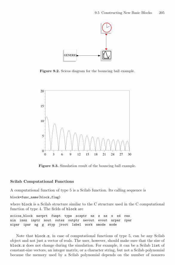
9.5 Constructing New Basic Blocks 205
GENERICGENERIC
Figure 9.2. Scicos diagram for the bouncing ball example.
0 3 6 9 12 15 18 21 24 27 300
5
10
15
20
+
Figure 9.3. Simulation result of the bouncing ball example.
Scilab Computational Functions
A computational function of type 5 is a Scilab function. Its calling sequence is
block=func_name(block,flag)
where block is a Scilab structure similar to the C structure used in the C computationalfunction of type 4. The fields of block are
scicos_block nevprt funpt type scsptr nz z nx x xd res
nin insz inptr nout outsz outptr nevout evout nrpar rpar
nipar ipar ng g ztyp jroot label work nmode mode
Note that block.z, in case of computational functions of type 5, can be any Scilabobject and not just a vector of reals. The user, however, should make sure that the size ofblock.z does not change during the simulation. For example, it can be a Scilab list ofconstant-size vectors, an integer matrix, or a character string, but not a Scilab polynomialbecause the memory used by a Scilab polynomial depends on the number of nonzero
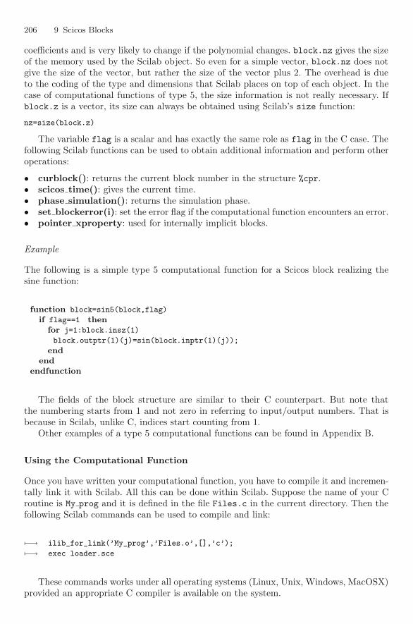
206 9 Scicos Blocks
coefficients and is very likely to change if the polynomial changes. block.nz gives the sizeof the memory used by the Scilab object. So even for a simple vector, block.nz does notgive the size of the vector, but rather the size of the vector plus 2. The overhead is dueto the coding of the type and dimensions that Scilab places on top of each object. In thecase of computational functions of type 5, the size information is not really necessary. Ifblock.z is a vector, its size can always be obtained using Scilab’s size function:
nz=size(block.z)
The variable flag is a scalar and has exactly the same role as flag in the C case. Thefollowing Scilab functions can be used to obtain additional information and perform otheroperations:
• curblock(): returns the current block number in the structure %cpr.• scicos time(): gives the current time.• phase simulation(): returns the simulation phase.• set blockerror(i): set the error flag if the computational function encounters an error.• pointer xproperty: used for internally implicit blocks.
Example
The following is a simple type 5 computational function for a Scicos block realizing thesine function:
function block=sin5(block,flag)
if flag==1 thenfor j=1:block.insz(1)
block.outptr(1)(j)=sin(block.inptr(1)(j));
endend
endfunction
The fields of the block structure are similar to their C counterpart. But note thatthe numbering starts from 1 and not zero in referring to input/output numbers. That isbecause in Scilab, unlike C, indices start counting from 1.
Other examples of a type 5 computational functions can be found in Appendix B.
Using the Computational Function
Once you have written your computational function, you have to compile it and incremen-tally link it with Scilab. All this can be done within Scilab. Suppose the name of your Croutine is My prog and it is defined in the file Files.c in the current directory. Then thefollowing Scilab commands can be used to compile and link:
�−→ ilib_for_link(’My_prog’,’Files.o’,[],’c’);
�−→ exec loader.sce
These commands works under all operating systems (Linux, Unix, Windows, MacOSX)provided an appropriate C compiler is available on the system.

9.6 Constructing and Loading a New Palette 207
CBlock2
As we have seen in the previous section, if you are developing a new C computationalfunction, in order to use it in Scicos, you have to compile it and incrementally link itwith Scilab before launching Scicos. You also need an interfacing function (or you coulduse the GENERIC block). The CBlock2 block provides an alternative to this. It allows youto write your computational function on-line. The text is stored in the block structureand the compilation and linking are done automatically. The block also provides a genericinterfacing function. The main advantage of using CBlock2 is that the C computationalfunction is included in the block and thus in the diagram structure. This means that theScicos diagram is self-contained and can be used on different operating systems. The onlydrawback is that the diagram works only if there is an appropriate C compiler availableon the operating system being used. If the computational function is used directly withoutCBlock2, then dll libraries can be provided along with the diagram and the block willfunction even if no compiler is available. It also means that the source of the computationalfunction need not be made available. This could be of interest for commercial toolboxes.
9.5.3 Saving New Blocks
New blocks can be used in a Scicos diagram using the AddNewBlock menu by giving thename of the corresponding interfacing function. However, it is a lot more convenient toplace new blocks in user palettes. A palette is simply a Scicos diagram from which theuser can copy blocks into the Scicos editor. To edit a palette, for example to add a newblock, the palette should be loaded as a diagram, edited, and saved.
9.6 Constructing and Loading a New Palette
A palette can be defined if the computational and interfacing functions associated to allof its blocks are available. Suppose we want to construct a palette named foo and we haveplaced inside the directory /home/basile/foo the C files containing the computationalfunctions foo blk1 through foo blk5 and Scilab interfacing functions associated to theblocks to be placed in the palette. Each interfacing function is supposed to be in a filewith extension .sci bearing its name.
The C and Scilab files can be compiled and the corresponding libraries generated bythe appropriate commands (usually ilib for link for C functions and genlib for Scilabfunctions). These commands can be placed in a file called builder.sce. The following isthe content of a builder.sce for compiling the C functions:
�−→ comp_fun_lst=[’foo_blk1’,’foo_blk2’,’foo_blk3’,’foo_blk4’,’foo_blk5’];
�−→ c_prog_lst=listfiles(’*.c’); //list of C programs in the directory
�−→ prog_lst=strsubst(c_prog_lst,’.c’,’.o’);
�−→ ilib_for_link(comp_fun,prog_lst,’c’); // compile and generate loader
�−→ genlib(’lib_foo’,pwd()); // compile macros and generate lib
Note that to execute this file, the current directory must be foo. The Scilab functiongenlib can be used to construct lib associated to Scilab functions as usual. This can bedone by the builder.sce function as well.
This script needs to be executed only once. It generates the libraries but does not loadthem. Loading of the interfacing functions can be done with the command load(’lib’)and linking the computational functions done with exec(’loader.sce’).
208 9 Scicos Blocks
At this point, the palette foo can be edited and saved in foo.cos or foo.cosf. Blocksare placed in the diagram using the Add New Block functionality.
The palette can also be constructed using the create palette Scilab function. Forthat, all the files containing the interfacing functions associated with the blocks in thepalette should be placed in a directory. Each file must bear the name of the function withthe extension .sci, as usual. Then the function create palette, called with argumentthe path to this directory, creates the Scicos diagram of the palette. For example, if thedirectory /home/basile/foo contains the interfacing function files, the command
�−→ create_palette(’/home/basile/foo’);
creates a Scicos diagram (palette) foo.cosf and places it in /home/basile/foo.To load the palette, we can now construct a loader.sce script as follows
�−→ load(’lib’) // loads the interfacing functions
�−→ scicos_pal($+1,1)=’foo’; //adding the palette to the list
�−→ scicos_pal($+1,2)=’/home/basile/foo/foo.cosf’;
It is good programming practice to provide with each palette the builder and theloader scripts. These scripts may also be used for creating and loading manual pages forthe blocks.
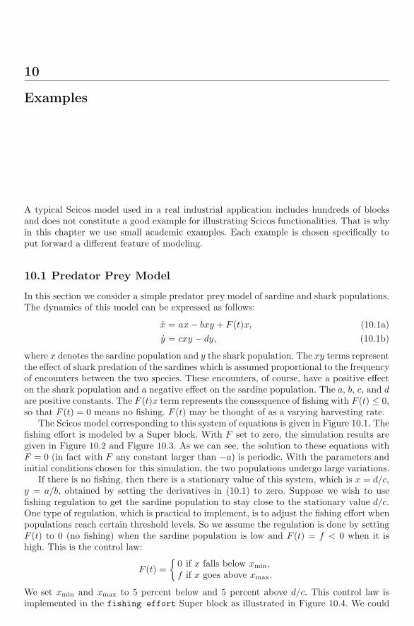
10
Examples
A typical Scicos model used in a real industrial application includes hundreds of blocksand does not constitute a good example for illustrating Scicos functionalities. That is whyin this chapter we use small academic examples. Each example is chosen specifically toput forward a different feature of modeling.
10.1 Predator Prey Model
In this section we consider a simple predator prey model of sardine and shark populations.The dynamics of this model can be expressed as follows:
x = ax − bxy + F (t)x, (10.1a)y = cxy − dy, (10.1b)
where x denotes the sardine population and y the shark population. The xy terms representthe effect of shark predation of the sardines which is assumed proportional to the frequencyof encounters between the two species. These encounters, of course, have a positive effecton the shark population and a negative effect on the sardine population. The a, b, c, and dare positive constants. The F (t)x term represents the consequence of fishing with F (t) ≤ 0,so that F (t) = 0 means no fishing. F (t) may be thought of as a varying harvesting rate.
The Scicos model corresponding to this system of equations is given in Figure 10.1. Thefishing effort is modeled by a Super block. With F set to zero, the simulation results aregiven in Figure 10.2 and Figure 10.3. As we can see, the solution to these equations withF = 0 (in fact with F any constant larger than −a) is periodic. With the parameters andinitial conditions chosen for this simulation, the two populations undergo large variations.
If there is no fishing, then there is a stationary value of this system, which is x = d/c,y = a/b, obtained by setting the derivatives in (10.1) to zero. Suppose we wish to usefishing regulation to get the sardine population to stay close to the stationary value d/c.One type of regulation, which is practical to implement, is to adjust the fishing effort whenpopulations reach certain threshold levels. So we assume the regulation is done by settingF (t) to 0 (no fishing) when the sardine population is low and F (t) = f < 0 when it ishigh. This is the control law:
F (t) ={
0 if x falls below xmin,f if x goes above xmax.
We set xmin and xmax to 5 percent below and 5 percent above d/c. This control law isimplemented in the fishing effort Super block as illustrated in Figure 10.4. We could
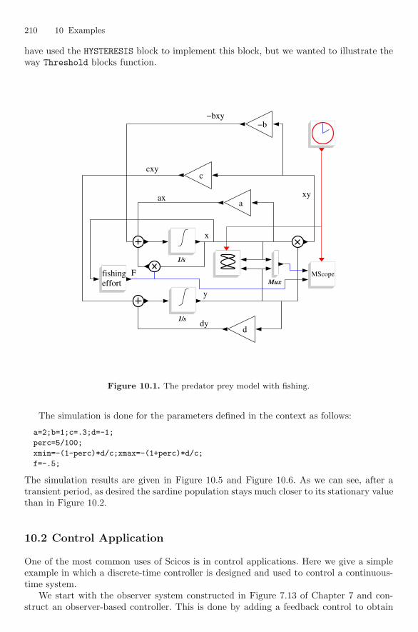
210 10 Examples
have used the HYSTERESIS block to implement this block, but we wanted to illustrate theway Threshold blocks function.
1/s
1/s
cc
−b−b
dd
aa
x
y
xy
−bxy
cxy
F
ax
dy
MScopeMScopeeffortfishingeffortfishing
Mux
Figure 10.1. The predator prey model with fishing.
The simulation is done for the parameters defined in the context as follows:
a=2;b=1;c=.3;d=-1;
perc=5/100;
xmin=-(1-perc)*d/c;xmax=-(1+perc)*d/c;
f=-.5;
The simulation results are given in Figure 10.5 and Figure 10.6. As we can see, after atransient period, as desired the sardine population stays much closer to its stationary valuethan in Figure 10.2.
10.2 Control Application
One of the most common uses of Scicos is in control applications. Here we give a simpleexample in which a discrete-time controller is designed and used to control a continuous-time system.
We start with the observer system constructed in Figure 7.13 of Chapter 7 and con-struct an observer-based controller. This is done by adding a feedback control to obtain
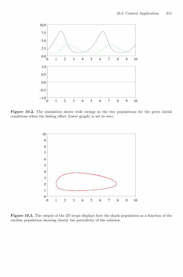
10.2 Control Application 211
0 1 2 3 4 5 6 7 8 9 100.0
2.5
5.0
7.5
10.0
+
0 1 2 3 4 5 6 7 8 9 10−1.0
−0.5
0.0
0.5
1.0
+
Figure 10.2. The simulation shows wide swings in the two populations for the given initialconditions when the fishing effort (lower graph) is set to zero.
0 1 2 3 4 5 6 7 8 9 100
1
2
3
4
5
6
7
8
9
10
+
Figure 10.3. The output of the 2D scope displays here the shark population as a function of thesardine population showing clearly the periodicity of the solution.
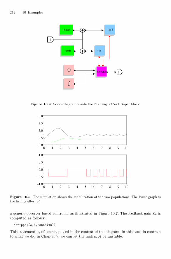
212 10 Examples
−xmax−xmax
−xmin−xmin
00
ff
SelectorSelector 11
11
− to + − to +
+ to − + to −
Figure 10.4. Scicos diagram inside the fishing effort Super block.
0 1 2 3 4 5 6 7 8 9 100.0
2.5
5.0
7.5
10.0
+
0 1 2 3 4 5 6 7 8 9 10−1.0
−0.5
0.0
0.5
1.0
+
Figure 10.5. The simulation shows the stabilization of the two populations. The lower graph isthe fishing effort F .
a generic observer-based controller as illustrated in Figure 10.7. The feedback gain Kc iscomputed as follows:
Kc=-ppol(A,B,-ones(x0))
This statement is, of course, placed in the context of the diagram. In this case, in contrastto what we did in Chapter 7, we can let the matrix A be unstable.
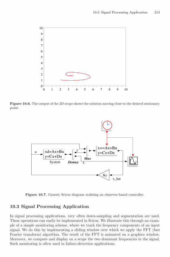
10.3 Signal Processing Application 213
0 1 2 3 4 5 6 7 8 9 100
1
2
3
4
5
6
7
8
9
10
+
Figure 10.6. The output of the 2D scope shows the solution moving close to the desired stationarypoint.
y=Cx+Duxd=Ax+Buy=Cx+Duxd=Ax+Bu
Demux
y=Cx+Dux+=Ax+Buy=Cx+Dux+=Ax+Bu
KcKc
MuxSystem x
u
x_hat
y
Figure 10.7. Generic Scicos diagram realizing an observer-based controller.
10.3 Signal Processing Application
In signal processing applications, very often down-sampling and segmentation are used.These operations can easily be implemented in Scicos. We illustrate this through an exam-ple of a simple monitoring scheme, where we track the frequency components of an inputsignal. We do this by implementing a sliding window over which we apply the FFT (fastFourier transform) algorithm. The result of the FFT is animated on a graphics window.Moreover, we compute and display on a scope the two dominant frequencies in the signal.Such monitoring is often used in failure-detection applications.
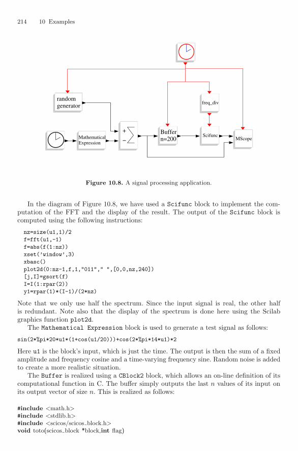
214 10 Examples
n=200Buffern=200Buffer
MScopeMScopeScifuncScifunc
freq_divfreq_div
ExpressionMathematicalExpressionMathematical
+
−
+
−
generatorrandomgeneratorrandom
Figure 10.8. A signal processing application.
In the diagram of Figure 10.8, we have used a Scifunc block to implement the com-putation of the FFT and the display of the result. The output of the Scifunc block iscomputed using the following instructions:
nz=size(u1,1)/2
f=fft(u1,-1)
f=abs(f(1:nz))
xset(’window’,3)
xbasc()
plot2d(0:nz-1,f,1,"011"," ",[0,0,nz,240])
[j,I]=gsort(f)
I=I(1:rpar(2))
y1=rpar(1)*(I-1)/(2*nz)
Note that we only use half the spectrum. Since the input signal is real, the other halfis redundant. Note also that the display of the spectrum is done here using the Scilabgraphics function plot2d.
The Mathematical Expression block is used to generate a test signal as follows:
sin(2*%pi*20*u1*(1+cos(u1/20)))+cos(2*%pi*14*u1)*2
Here u1 is the block’s input, which is just the time. The output is then the sum of a fixedamplitude and frequency cosine and a time-varying frequency sine. Random noise is addedto create a more realistic situation.
The Buffer is realized using a CBlock2 block, which allows an on-line definition of itscomputational function in C. The buffer simply outputs the last n values of its input onits output vector of size n. This is realized as follows:
#include <math.h>#include <stdlib.h>#include <scicos/scicos block.h>void toto(scicos block *block,int flag)
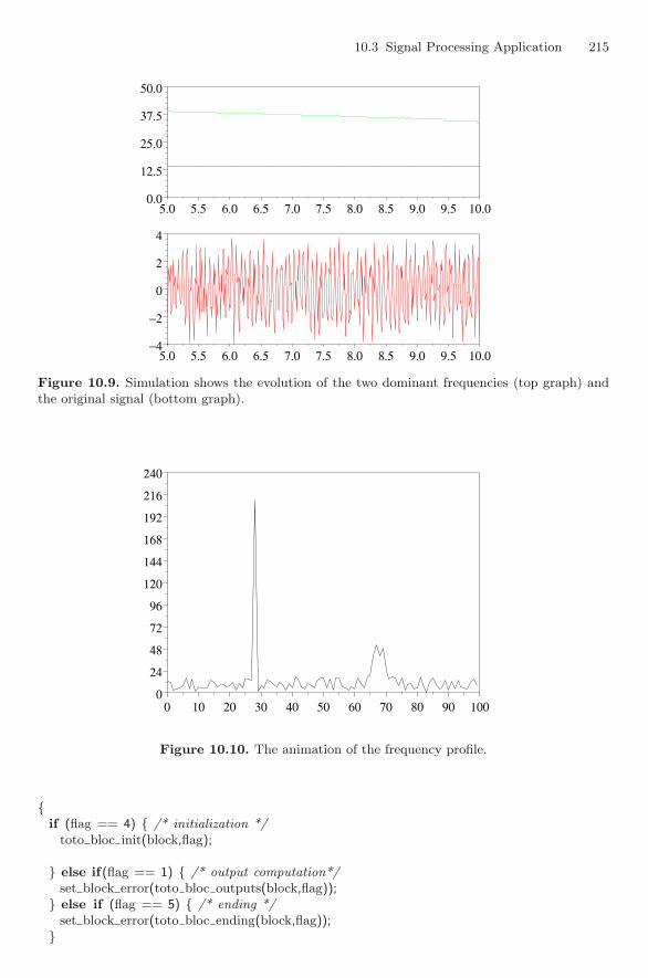
10.3 Signal Processing Application 215
5.0 5.5 6.0 6.5 7.0 7.5 8.0 8.5 9.0 9.5 10.00.0
12.5
25.0
37.5
50.0
+
5.0 5.5 6.0 6.5 7.0 7.5 8.0 8.5 9.0 9.5 10.0−4
−2
0
2
4
+
Figure 10.9. Simulation shows the evolution of the two dominant frequencies (top graph) andthe original signal (bottom graph).
0 10 20 30 40 50 60 70 80 90 1000
24
48
72
96
120
144
168
192
216
240
Figure 10.10. The animation of the frequency profile.
{if (flag == 4) { /* initialization */
toto bloc init(block,flag);
} else if(flag == 1) { /* output computation*/set block error(toto bloc outputs(block,flag));
} else if (flag == 5) { /* ending */set block error(toto bloc ending(block,flag));
}
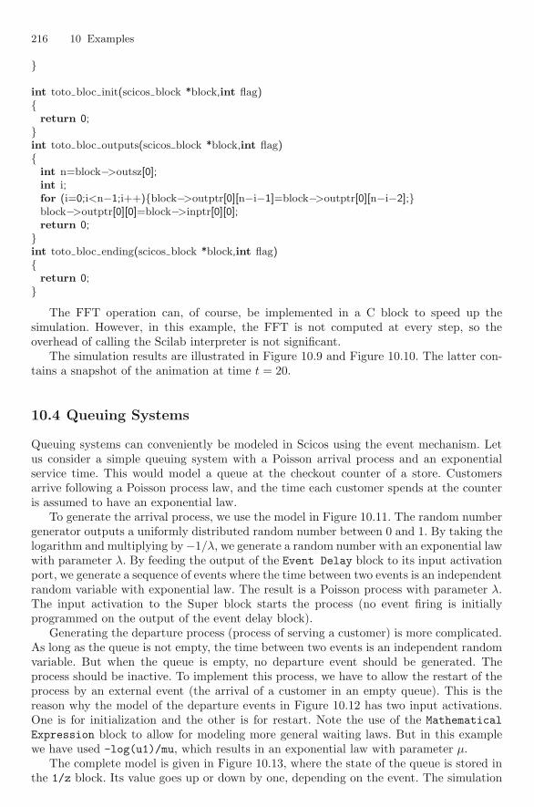
216 10 Examples
}
int toto bloc init(scicos block *block,int flag){
return 0;}int toto bloc outputs(scicos block *block,int flag){
int n=block−>outsz[0];int i;for (i=0;i<n−1;i++){block−>outptr[0][n−i−1]=block−>outptr[0][n−i−2];}block−>outptr[0][0]=block−>inptr[0][0];return 0;
}int toto bloc ending(scicos block *block,int flag){
return 0;}
The FFT operation can, of course, be implemented in a C block to speed up thesimulation. However, in this example, the FFT is not computed at every step, so theoverhead of calling the Scilab interpreter is not significant.
The simulation results are illustrated in Figure 10.9 and Figure 10.10. The latter con-tains a snapshot of the animation at time t = 20.
10.4 Queuing Systems
Queuing systems can conveniently be modeled in Scicos using the event mechanism. Letus consider a simple queuing system with a Poisson arrival process and an exponentialservice time. This would model a queue at the checkout counter of a store. Customersarrive following a Poisson process law, and the time each customer spends at the counteris assumed to have an exponential law.
To generate the arrival process, we use the model in Figure 10.11. The random numbergenerator outputs a uniformly distributed random number between 0 and 1. By taking thelogarithm and multiplying by −1/λ, we generate a random number with an exponential lawwith parameter λ. By feeding the output of the Event Delay block to its input activationport, we generate a sequence of events where the time between two events is an independentrandom variable with exponential law. The result is a Poisson process with parameter λ.The input activation to the Super block starts the process (no event firing is initiallyprogrammed on the output of the event delay block).
Generating the departure process (process of serving a customer) is more complicated.As long as the queue is not empty, the time between two events is an independent randomvariable. But when the queue is empty, no departure event should be generated. Theprocess should be inactive. To implement this process, we have to allow the restart of theprocess by an external event (the arrival of a customer in an empty queue). This is thereason why the model of the departure events in Figure 10.12 has two input activations.One is for initialization and the other is for restart. Note the use of the MathematicalExpression block to allow for modeling more general waiting laws. But in this examplewe have used -log(u1)/mu, which results in an exponential law with parameter μ.
The complete model is given in Figure 10.13, where the state of the queue is stored inthe 1/z block. Its value goes up or down by one, depending on the event. The simulation
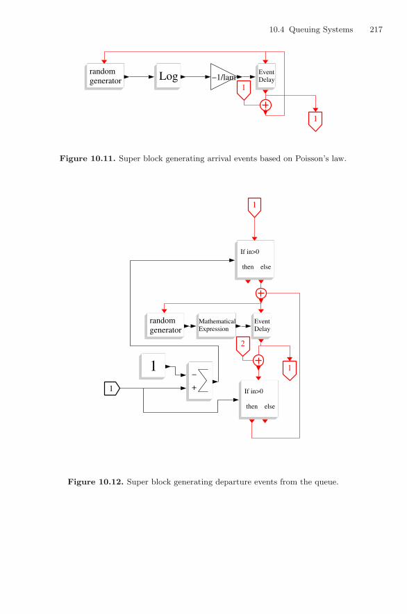
10.4 Queuing Systems 217
generatorrandomgeneratorrandom
−1/lam−1/lamLogLog DelayEventDelayEvent
11
11
Figure 10.11. Super block generating arrival events based on Poisson’s law.
then else
If in>0
then else
If in>0
ExpressionMathematicalExpressionMathematical
DelayEventDelayEvent
then else
If in>0
then else
If in>0
generatorrandomgeneratorrandom
−
+
−
+
11
11
11
11
22
Figure 10.12. Super block generating departure events from the queue.
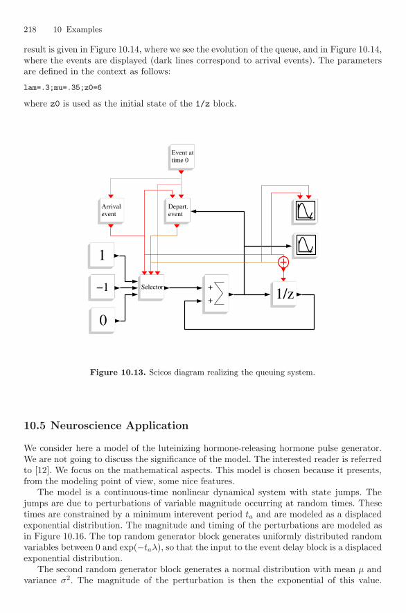
218 10 Examples
result is given in Figure 10.14, where we see the evolution of the queue, and in Figure 10.14,where the events are displayed (dark lines correspond to arrival events). The parametersare defined in the context as follows:
lam=.3;mu=.35;z0=6
where z0 is used as the initial state of the 1/z block.
11
SelectorSelector
1/z1/z+
+
+
+
−1−1
eventArrivaleventArrival
eventDepart.eventDepart.
time 0Event attime 0Event at
00
Figure 10.13. Scicos diagram realizing the queuing system.
10.5 Neuroscience Application
We consider here a model of the luteinizing hormone-releasing hormone pulse generator.We are not going to discuss the significance of the model. The interested reader is referredto [12]. We focus on the mathematical aspects. This model is chosen because it presents,from the modeling point of view, some nice features.
The model is a continuous-time nonlinear dynamical system with state jumps. Thejumps are due to perturbations of variable magnitude occurring at random times. Thesetimes are constrained by a minimum interevent period ta and are modeled as a displacedexponential distribution. The magnitude and timing of the perturbations are modeled asin Figure 10.16. The top random generator block generates uniformly distributed randomvariables between 0 and exp(−taλ), so that the input to the event delay block is a displacedexponential distribution.
The second random generator block generates a normal distribution with mean μ andvariance σ2. The magnitude of the perturbation is then the exponential of this value.
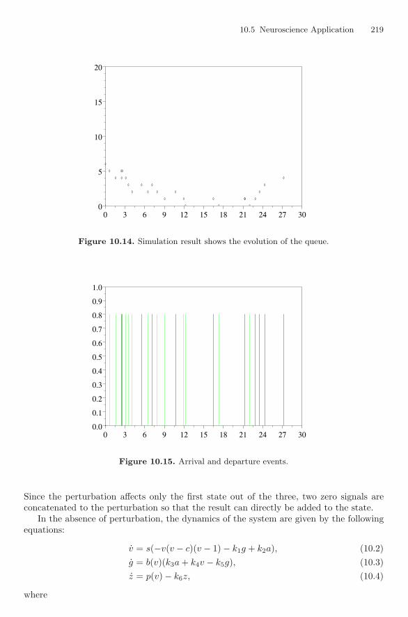
10.5 Neuroscience Application 219
0 3 6 9 12 15 18 21 24 27 300
5
10
15
20
+
◊
◊
◊
◊
◊
◊
◊
◊
◊
◊
◊
◊
◊
◊
◊
◊
◊
◊
◊
◊◊
◊
◊
◊
◊
◊
Figure 10.14. Simulation result shows the evolution of the queue.
0 3 6 9 12 15 18 21 24 27 300.0
0.1
0.2
0.3
0.4
0.5
0.6
0.7
0.8
0.9
1.0
+
Figure 10.15. Arrival and departure events.
Since the perturbation affects only the first state out of the three, two zero signals areconcatenated to the perturbation so that the result can directly be added to the state.
In the absence of perturbation, the dynamics of the system are given by the followingequations:
v = s(−v(v − c)(v − 1) − k1g + k2a), (10.2)g = b(v)(k3a + k4v − k5g), (10.3)z = p(v) − k6z, (10.4)
where
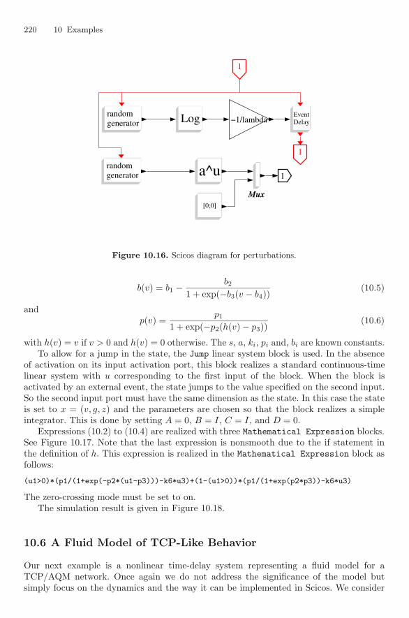
220 10 Examples
generatorrandomgeneratorrandom
DelayEventDelayEvent
11
11
11a^ua^ugeneratorrandomgeneratorrandom
LogLog −1/lambda−1/lambda
Mux[0;0][0;0]
Figure 10.16. Scicos diagram for perturbations.
b(v) = b1 − b2
1 + exp(−b3(v − b4))(10.5)
andp(v) =
p1
1 + exp(−p2(h(v) − p3))(10.6)
with h(v) = v if v > 0 and h(v) = 0 otherwise. The s, a, ki, pi and, bi are known constants.To allow for a jump in the state, the Jump linear system block is used. In the absence
of activation on its input activation port, this block realizes a standard continuous-timelinear system with u corresponding to the first input of the block. When the block isactivated by an external event, the state jumps to the value specified on the second input.So the second input port must have the same dimension as the state. In this case the stateis set to x = (v, g, z) and the parameters are chosen so that the block realizes a simpleintegrator. This is done by setting A = 0, B = I, C = I, and D = 0.
Expressions (10.2) to (10.4) are realized with three Mathematical Expression blocks.See Figure 10.17. Note that the last expression is nonsmooth due to the if statement inthe definition of h. This expression is realized in the Mathematical Expression block asfollows:
(u1>0)*(p1/(1+exp(-p2*(u1-p3)))-k6*u3)+(1-(u1>0))*(p1/(1+exp(p2*p3))-k6*u3)
The zero-crossing mode must be set to on.The simulation result is given in Figure 10.18.
10.6 A Fluid Model of TCP-Like Behavior
Our next example is a nonlinear time-delay system representing a fluid model for aTCP/AQM network. Once again we do not address the significance of the model butsimply focus on the dynamics and the way it can be implemented in Scicos. We consider

10.7 Interactive GUI 221
(A,B,C,D)Jump(A,B,C,D)Jump+
+
+
+MScopeMScopeDemuxDemux
ExpressionMathematicalExpressionMathematical
ExpressionMathematicalExpressionMathematical
ExpressionMathematicalExpressionMathematical
Mux
generatorPulsegeneratorPulse
Figure 10.17. Scicos diagram realizing the luteinizing hormone-releasing hormone pulse gener-ator.
this system to show how delay differential systems can be modeled. We use one of themodels studied in [29]:
W (t) =1R
− W (t)W (t − R)2R
KQ(t − R), (10.7)
Q(t) =
{N W (t)
R − C, Q > 0,
max(N W (t)R − C, 0), Q = 0.
(10.8)
The Scicos diagram realizing this system is given in Figure 10.19. The continuous-timefixed delay blocks are used to implement the delay. The content of the MathematicalExpression block is
(u2==0)*max(N*u1/R-C,0)+(u2>0)*(N*u1/R-C)
The simulation result is displayed in the 2D scope, where W is plotted as a functionof Q. Note that the result is compatible with that obtained in [32].
10.7 Interactive GUI
In some applications, it is desirable to have the possibility of adjusting certain system pa-rameters during the simulation without having to stop and restart the simulation process.We consider here a simple example to illustrate how this can be done. The technique usedhere can be used to construct sophisticated control panels for controlling simulations.
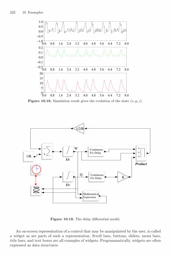
222 10 Examples
0.0 0.8 1.6 2.4 3.2 4.0 4.8 5.6 6.4 7.2 8.0−1.0−0.5
0.00.51.0
+
0.0 0.8 1.6 2.4 3.2 4.0 4.8 5.6 6.4 7.2 8.0−0.2−0.1
0.00.10.2
+
0.0 0.8 1.6 2.4 3.2 4.0 4.8 5.6 6.4 7.2 8.005
101520
+
Figure 10.18. Simulation result gives the evolution of the state (v, g, z).
1/s
1/s
ExpressionMathematicalExpressionMathematical
Fix DelayContinuousFix DelayContinuous
Fix DelayContinuousFix DelayContinuous
Product
***
***
KK
1/2/R1/2/R
−
+
−
+1/R1/R
W
Q
Figure 10.19. The delay differential model.
An on-screen representation of a control that may be manipulated by the user, is calleda widget as are parts of such a representation. Scroll bars, buttons, sliders, menu bars,title bars, and text boxes are all examples of widgets. Programmatically, widgets are oftenexpressed as data structures.
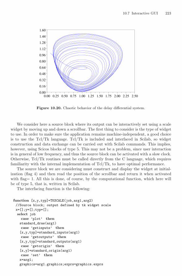
10.7 Interactive GUI 223
0.00 0.25 0.50 0.75 1.00 1.25 1.50 1.75 2.00 2.25 2.500.00
0.16
0.32
0.48
0.64
0.80
0.96
1.12
1.28
1.44
1.60
+
Figure 10.20. Chaotic behavior of the delay differential system.
We consider here a source block where its output can be interactively set using a scalewidget by moving up and down a scrollbar. The first thing to consider is the type of widgetto use. In order to make sure the application remains machine-independent, a good choiceis to use the Tcl/Tk language. Tcl/Tk is included and interfaced in Scilab, so widgetconstruction and data exchange can be carried out with Scilab commands. This implies,however, using Scicos blocks of type 5. This may not be a problem, since user interactionis in general of low frequency, and thus the source block can be activated with a slow clock.Otherwise, Tcl/Tk routines must be called directly from the C language, which requiresfamiliarity with the internal implementation of Tcl/Tk, to have optimal performance.
The source block we are considering must construct and display the widget at initial-ization (flag 4) and then read the position of the scrollbar and return it when activatedwith flag= 1. All this is done, of course, by the computational function, which here willbe of type 5, that is, written in Scilab.
The interfacing function is the following:
function [x,y,typ]=TKSCALE(job,arg1,arg2)
//Source block; output defined by tk widget scale
x=[];y=[];typ=[];
select job
case ’plot’ thenstandard_draw(arg1)
case ’getinputs’ then[x,y,typ]=standard_inputs(arg1)
case ’getoutputs’ then[x,y,typ]=standard_outputs(arg1)
case ’getorigin’ then[x,y]=standard_origin(arg1)
case ’set’ thenx=arg1;
graphics=arg1.graphics;exprs=graphics.exprs
224 10 Examples
model=arg1.model;
[ok,a,b,f,exprs]=getvalue(’Set scale block parameters’,..
[’Min value’;’Max value’;’Normalization’],..
list(’vec’,1,’vec’,1,’vec’,1),exprs)
// tk widget returns a scalar, the value is divided by
// Normalization factor
if ok thengraphics.exprs=exprs
model.rpar=[a;b;f]
x.graphics=graphics;x.model=model
endcase ’define’ thena=0;b=100;f=1;// default parameter values
model=scicos_model()
model.sim=list(’tkscaleblk’,5)
model.out=1
model.evtin=1
model.rpar=[a;b;f]
model.blocktype=’d’
model.dep_ut=[%f %f]
exprs=[sci2exp(a);sci2exp(b);sci2exp(f)]
gr_i=[’xstringb(orig(1),orig(2),’’TK Scale’’,sz(1),sz(2),’’fill’’)’]
x=standard_define([3 2],model,exprs,gr_i)
endendfunction
Note that the block has three parameters: the first two are the minimum value and themaximum value of the scale. The last is a normalization factor. The output of the block isnormalized by dividing the scale value by this factor. This allows, in particular, the displayof only integer scale values inside the widget.
The computational function is the following:
function block=tkscaleblk(block,flag)
blknb=string(curblock())
if flag==4 thencur=%cpr.corinv(curblock())
if size(cur,’*’)==1 then // open widget only if the block
// is in main Scicos editor window
o=scs_m.objs(cur).graphics.orig;
sz=scs_m.objs(cur).graphics.sz
pos=point2pixel(1000,o)
pos(1)=pos(1)+width2pixel(1000,sz(1)) // widget position
geom=’wm geometry $w +’+string(pos(1))+’+’+ string(pos(2));
title=block.label
if title==[] then title="TK source", endtit=’wm title $w Scale’+blknb // write block label
bounds=block.rpar(1:2)
bnds=’-from ’+string(bounds(1))+’ -to ’+string(bounds(2))
cmd=’-command ""f’+blknb+’ $w.frame.scale""’
lab=’-label ""’+title+’""’;
L=’-length 100’
I=’-tickinterval ’+string((bounds(2)-bounds(1))/4)
scale=strcat([’scale $w.frame.scale -orient vertical’,..
10.7 Interactive GUI 225
lab,bnds,cmd,L,I],’ ’)
initial=mean(bounds) // initial value is the mean
txt=[’set w0.vscale’+blknb;
’set y’+blknb+’ 0’;
’catch destroy $w’;
’toplevel $w’;
tit
geom
’frame $w.frame -borderwidth 10’;
’pack $w.frame’;
scale
’frame $w.frame.right -borderwidth 15’;
’pack $w.frame.scale -side left -anchor ne’;
’$w.frame.scale set ’+string(initial);
’proc f’+blknb+’ w height global y’+blknb+’;set y’+blknb+’ $height’
];
TCL_EvalStr(txt) // call TCL interpretor to create widget
block.outptr(1)=mean(block.rpar(1:2))/block.rpar(3);
endelseif flag==1 then // evaluate output during simulation
block.outptr(1)=evstr(TCL_GetVar(’y’+blknb))/block.rpar(3);
endendfunction
The block number (returned by the function curblock) is used to customize Tcl variablenames to make sure that if two of these blocks are used in the same diagram, they createdifferent widgets. The position of the widget is computed so that it is placed next to thecorresponding block in the Scicos diagram (it can be moved subsequently by the user). Thecomplete Tcl text for the construction of the widget is sent to the Tcl interpreter using theTCL EvalStr command. The Tcl procedure defined in the program sets the variable yN(where N is the block number) to the value designated by the position of the scrollbar inthe scale. This variable is returned from the Tcl environment to Scilab using the commandTCL GetVar in the case of flag= 1. It is then normalized and returned as the output of theblock.
The source block TKSCALE can be used, for example, to adjust manually the parametersof a PD controller. This is done in the diagram illustrated in Figure 10.21. The clock periodactivating the square-wave generator is set to half that of the refresh period of the scopeso that the output of the generator, displayed as the first curve on the scope, remainsalways the same, that is, −1 up to the middle of the screen and then 1. The output of theplant is changed as the user moves up and down the scrollbars in the GUI boxes. See thesimulation result in Figure 10.22.
Various Tcl/Tk widgets can be used to display simulation results and even to constructa scope using Tk Canvas. It is not difficult to imagine the construction of sophisticatedcontrol panels, for example, the instrumentation panel of a car in Tcl/Tk to be used witha simulation model of the car. This can be done even if the model is simulated in batchmode.
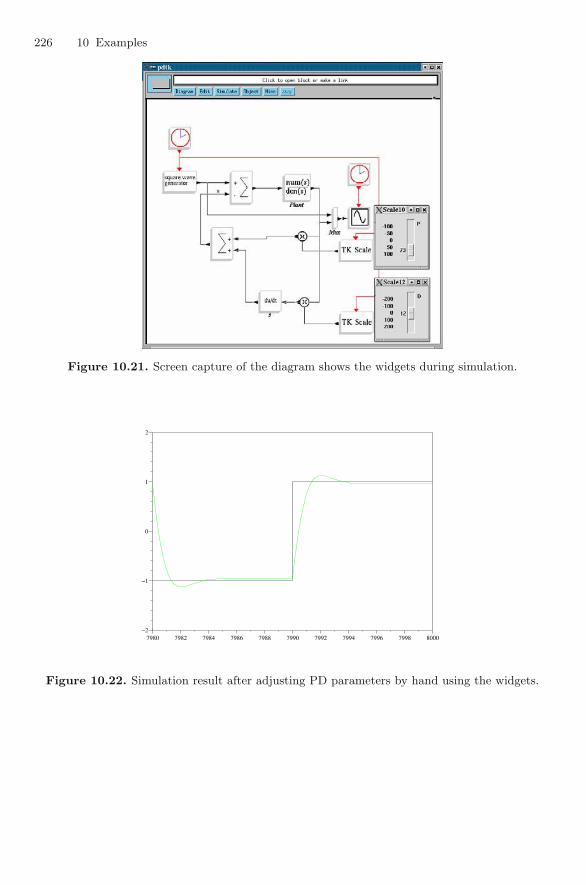
226 10 Examples
Figure 10.21. Screen capture of the diagram shows the widgets during simulation.
7980 7982 7984 7986 7988 7990 7992 7994 7996 7998 8000−2
−1
0
1
2
+
Figure 10.22. Simulation result after adjusting PD parameters by hand using the widgets.

11
Batch Processing in Scilab
Having Scicos live within Scilab is very useful because it allows the interaction of the twoin many different ways, thereby mutually enriching their functionalities. We have alreadyseen that Scicos relies heavily on the Scilab language. The Scicos editor is, for example,fully written in Scilab, making it easy for the user to add new functionalities or customizeexisting ones. We have also seen that the interfacing functions of all Scicos blocks areScilab functions using only standard Scilab commands. For example, to define a block’sicon we use standard Scilab graphics commands. But perhaps the most important aspectof having access to Scilab in Scicos is the ability to use Scilab commands from specializedtoolboxes, such as Signal Processing, Control and Optimization, in the construction ofScicos blocks.
In this chapter we look at the ways Scicos simulations can be performed and usedin Scilab. We have already seen that Scilab can be used for postprocessing Scicos simu-lation results, but here we look at ways of piloting Scicos functionalities through Scilabcommands.
In doing modeling and simulation work, very often one needs to perform multiplesimulations either for adjusting or optimizing model parameters, or for testing the modelon multiple data sets, or for performing simulation-based statistical analyses. Monte Carlotechniques are one example. In such cases, Scicos simulations should be carried out in batchmode. In the Scilab/Scicos environment, this can be done within the Scilab language,which not only can handle repetitive calls to the Scicos simulator by changing the valueof a parameter or the name of a file each time, but can also perform complicated analysesand make decisions on how to proceed with additional simulation runs.
11.1 Piloting Scicos via Scilab Commands
Having the Scicos editor written entirely in Scilab simplifies a great deal the piloting ofScicos commands from Scilab. Note, however, that the Scicos library is not loaded bydefault into the Scilab environment. So if you want to use any Scicos routines withinScilab, you must first load them as follows:
�−→ load SCI/macros/scicos/lib
228 11 Batch Processing in Scilab
if you are writing a Scilab function, you can place this instruction on top of it. Scicosblocks’ interfacing functions associated with the blocks inside Scicos palettes are not loadedautomatically either. If they are needed, they can be loaded as follows:
�−→ exec (loadpallibs,-1)
You can now use Scicos commands associated with each editor button. The name ofthe function is obtained from the text inside the button from which empty spaces, slashes,dots and dashes have been removed and an underscore has been added to the end. Forexample, the Scilab function associated with the button Save As is named SaveAs . It isdefined in the directory scilab/macros/scicos, like all other editor functions, and insidethe file SaveAs .sci.
Note, however, that using editor commands requires a good understanding of the datastructures and global variables used in the Scicos editor. Some of these functions re-quire that these variables be defined properly. In order to see how the editor functionsshould be called, we examine the scicos function. This function, which can be found inscilab/macros/auto/scicos.sci, is the main Scicos editor program and contains themain loop from which editor functions are called when the Scicos editor is active. Somedata structures used in this function are explained in Appendix A.
In many applications, however, it turns out that there is no need to access directlyevery editor command. The reason is that often when doing batch processing, we are onlyinterested in being able to change system parameters and running the simulation withthese new parameters. The Scilab function scicos simulate provides a generic way ofperforming batch simulation. This function is described in Section 11.1.2.
But first we describe scicosim, the basic Scilab function interfacing the Scicos simu-lator. This function can be used only if the Scicos diagram is compiled.
11.1.1 Function scicosim
The Scilab function scicosim is an interface to the Scicos simulator. To use this function,the Scicos diagram must be compiled because we need the compilation result %cpr. Theuser, however, need not be familiar with the compilation stage (information on that canbe found in Appendix A).
scicosim is called in three different ways. First it is called to initialize the simulation.This is done usually by the following Scilab command:
[state,t]=scicosim(state,0,tf,sim,’start’,tol)
The string start indicates that only the initialization must be performed. To run thesimulation and finish the simulation, the following corresponding calls are performed:
[state,t]=scicosim(state,t,tf,sim,’run’,tol)
and
[state,t]=scicosim(state,t,tf,sim,’finish’,tol)
The argument state initially contains the initial state of the system to be simulated(see Section A.2.3 for details). It contains, in particular, initial values of all the continuous-time and discrete-time states of all the blocks, the preprogrammed events, etc. state isboth an input and an output because it changes as the simulation goes on.

11.1 Piloting Scicos via Scilab Commands 229
The argument sim contains the scheduling tables needed by the simulator. These tablesare generated by the compiler and do not evolve during the simulation (see Section A.2.3for details).
The argument tf is the time up to which the simulation must run (not used withoptions start and finish). When scicosim is called with the run option, the simulationis performed up to time tf unless a pause or an error is encountered earlier. The outputargument t gives the actual ending time of the simulation. In most cases we have t equalto tf. The input argument t indicates the current time and is used only in the run case.Its value is, in general, 0 because Scicos simulations by default start at time 0. But if asimulation is to be continued by making other calls to scicosim with option run withoutstarting over, then the final time of the previous simulation (the output argument t ofprevious call to scicosim) must be used.
The argument tol is a vector containing various simulation parameters. It includes
1. atol: absolute tolerance (see Section 3.2.1).2. rtol: relative tolerance (see Section 3.2.1).3. ttol: minimum spacing in time between two events for the continuous-time solver to
be called. If two events are spaced closer than deltat in time, the solver is not calledand the continuous-time variables are supposed to remain constant over that period.
4. deltat: maximum time interval length used for each call to the continuous-time solver.If the next event is further in the future than deltat, the continuous-time solver iscalled more than once.
5. scale: sets the correspondence between simulation time and real time. If set to 1, oneunit of Scicos simulation time corresponds to one second. The solver is slowed downto achieve the desired correspondence. The default value 0 indicates that no slowingdown is to be performed and simulation runs at maximum speed.
6. hmax: maximum time step taken by the solver (see Section 3.2.1). The default value 0indicates no maximum being set.
To use scicosim, the variables state and sim must be available. The initial value ofstate and the value of sim are computed by the Scicos compiler from the Scicos diagram.It is possible to call the compiler from Scilab to construct these variables, but the simplersolution is to use the Scicos editor to construct them and save them to a file for future usein Scilab. This can be done as follows:
1. Use the Scicos editor to construct a block diagram and compile it.2. Save the compiled diagram in binary form (as a .cos file) using the Save or Save
As menu.3. In Scilab, load the saved file (say myfile.cos) using the load function:
load myfile.cos
You obtain Scilab variables scicos ver, scs m, and %cpr. scicos ver contains theversion number of Scicos that has created the diagram, scs m contains the Scicosdiagram, and %cpr contains the result of the compilation. It is this latter that is ofinterest to us for calling scicosim. In particular, %cpr is a Scilab structure containingstate, sim, cor, and corinv. Note that if the diagram is not compiled before beingsaved, then %cpr is an empty structure.
4. Extract state out of %cpr:
state=%cpr.state;
5. Define tol and tf, for example,
230 11 Batch Processing in Scilab
tf=1;
tol=[1.d-4,1.d-6,1.d-10,tf+1,0,0];
then call scicosim for initialization:
[state,t]=scicosim(state,0,tf,%cpr.sim,’start’,tol);
6. Then run the simulation from 0 to tf:
[state,t]=scicosim(state,t,tf,%cpr.sim,’run’,tol);
Successive such calls may be performed changing the final time tf before each call.7. End the simulation:
[state,t]=scicosim(state,t,tf,%cpr.sim,’finish’,tol);
Running Scicos simulations in Scilab in batch mode is useful if the user wants to performmultiple simulations by changing a parameter or an initial condition each time. All theparameters of the blocks in the diagram are in %cpr.sim. The initial conditions are instate. Note, however, that the change in the parameter should not require recompilation.For example, if one is testing the performance of a controller by changing its parameters,the order of the controller should not be modified, because this implies a change in thesize of a state, which in turn requires a partial recompilation since %cpr is no longer valid.
To change the parameter of a block, one must know the block number in the compiledstructure. This information can be obtained in the Scicos editor using the Get Info menuin the “Compiled structure index” field. This number specifies the order in which blocksare placed in %cpr fields. Note, however, that this number may change if the diagram isedited and recompiled.
This number can also be obtained in Scilab if a “label” has been associated with theblock of interest. Labels are available in %cpr.sim.labels as a vector. So, for example, ifthe label toto has been assigned to a block, the block number can be obtained using thecommand
k=find(%cpr.sim.labels==’toto’)
k is then the block number and can be used to examine and modify block parameters.Suppose the block labeled toto is a GAIN block. The parameters of the block that are theentries of the gain matrix, like all real parameters of all the blocks, are in %cpr.sim.rpar.The entries of the vector %cpr.sim.rpar that contain the parameter of block k can beobtained from %cpr.sim.rpptr, which is a vector of pointers to %cpr.sim.rpar. In par-ticular, let
idx=%cpr.sim.rpptr(k):%cpr.sim.rpptr(k+1)-1
Then idx contains the indices of %cpr.sim.rpar corresponding to the GAIN block:
gain_param=%cpr.sim.rpar(idx)
So if the objective is to run simulations for various gains, then before starting each simu-lation, the parameter must be set as follows:
%cpr.sim.rpar(idx)=new_gain_param
To change integer parameters, the procedure is identical except that the two vectorsto use are %cpr.sim.ipar and %cpr.sim.ipptr. For initial continuous-time and discrete-time states, the pointer vectors are respectively %cpr.sim.xptr and %cpr.sim.zptr, andthe values are found in %cpr.state.x and %cpr.state.z.
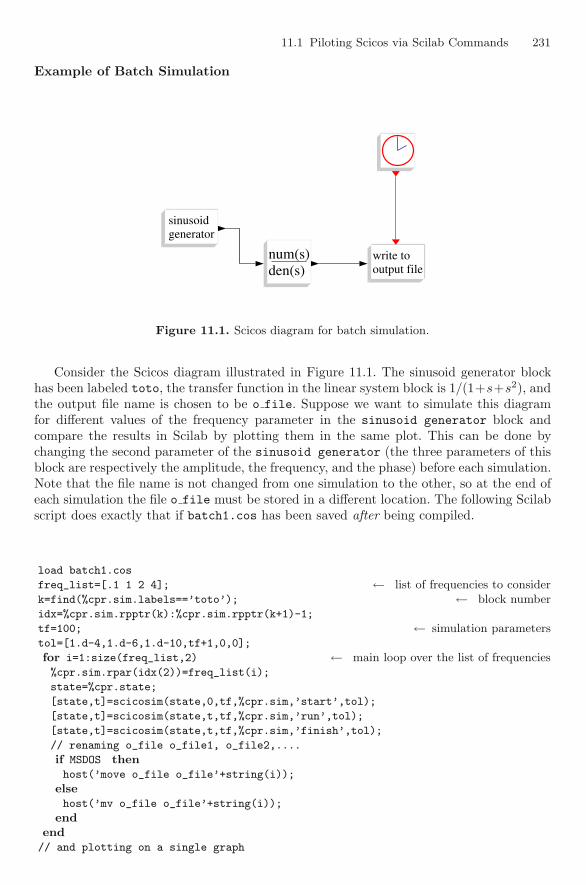
11.1 Piloting Scicos via Scilab Commands 231
Example of Batch Simulation
generatorsinusoidgeneratorsinusoid
output filewrite tooutput filewrite to
den(s)num(s)den(s)num(s)
Figure 11.1. Scicos diagram for batch simulation.
Consider the Scicos diagram illustrated in Figure 11.1. The sinusoid generator blockhas been labeled toto, the transfer function in the linear system block is 1/(1+s+s2), andthe output file name is chosen to be o file. Suppose we want to simulate this diagramfor different values of the frequency parameter in the sinusoid generator block andcompare the results in Scilab by plotting them in the same plot. This can be done bychanging the second parameter of the sinusoid generator (the three parameters of thisblock are respectively the amplitude, the frequency, and the phase) before each simulation.Note that the file name is not changed from one simulation to the other, so at the end ofeach simulation the file o file must be stored in a different location. The following Scilabscript does exactly that if batch1.cos has been saved after being compiled.
load batch1.cos
freq_list=[.1 1 2 4]; ← list of frequencies to considerk=find(%cpr.sim.labels==’toto’); ← block numberidx=%cpr.sim.rpptr(k):%cpr.sim.rpptr(k+1)-1;
tf=100; ← simulation parameterstol=[1.d-4,1.d-6,1.d-10,tf+1,0,0];
for i=1:size(freq_list,2) ← main loop over the list of frequencies%cpr.sim.rpar(idx(2))=freq_list(i);
state=%cpr.state;
[state,t]=scicosim(state,0,tf,%cpr.sim,’start’,tol);
[state,t]=scicosim(state,t,tf,%cpr.sim,’run’,tol);
[state,t]=scicosim(state,t,tf,%cpr.sim,’finish’,tol);
// renaming o_file o_file1, o_file2,....
if MSDOS thenhost(’move o_file o_file’+string(i));
elsehost(’mv o_file o_file’+string(i));
endend// and plotting on a single graph
232 11 Batch Processing in Scilab
xbasc()
for i=1:size(freq_list,2)
tx=read(’o_file’+string(i),-1,2); ← reading back the results of the simulationplot2d(tx(:,1),tx(:,2),i) ← and plotting on a single graph
end
In this example, we can avoid using the host command by changing the file namein the write to output file block. The file name is coded as an integer in the integerparameter vector of the block. To do so, however, we must know exactly where the nameappears in the vector. This information can be obtained by examining the interfacingfunction of the block. The integer coding of the name can be done using the Scilab functionstr2code. The function retrieving the name from the code is code2str. Note, however,that if we are to use this method to write into different files, all file names must have thesame length, unless %cpr.sim.ipptr is reconstructed. This is not recommended, especiallysince there is a more convenient way of handling such modifications, as we shall see in thenext section.
Finally, note that in this example the diagram contained no graphics displays such asa scope. This is often the case when one is doing batch processing. But sometimes it couldbe interesting to follow simulation results visually for debugging purposes. If a graphicsdisplay is used in the diagram, then make sure to switch to the old graphics style in Scilabbefore calling scicosim, because for the moment, Scicos displays use the old graphicsroutines. This can be done with the Scilab command
set(’old_style’,’on’)
11.1.2 Function scicos simulate
The scicos simulate function provides a convenient way of running Scicos simulations inScilab using the diagram’s data structure scs m. Unlike scicosim, scicos simulate doesnot require %cpr. The function scicos simulate handles automatically all the necessarycompilations in a transparent way.
In this case, model changes must be done by changing formal parameters defined nor-mally in the context; see Section 11.2.1 for information on formal parameters and theuse of context. Changing formal parameters not only is more convenient than directlychanging block parameters, it also allows for more general changes. For example, it is morenatural in the case of a linear system block, specified in terms of a transfer function, tospecify the new polynomials representing the transfer function’s numerator and denomina-tor than it is to change directly the matrices of the state-space representation. Moreover,by changing the transfer function, the order of the linear system and thus the size of itssystem matrices can vary.
In this case the scicos simulate function performs automatically the necessary (par-tial) recompilation.
The calling sequence of this function is as follows:
Info=scicos_simulate(scs_m,Info[,%scicos_context][,flag]);
The arguments %scicos context and flag are optional.
• scs m: scicos diagram, obtained for example by the instruction load mydiag.cos. Notethat the diagram mydiag need not be compiled because we do not make use of %cpr.The Scicos version of mydiag.cos must be the current version. If not (i.e., if the diagramhas been saved by an old version of Scicos), you must use the Scicos editor to load andsave. The save will be done automatically in the current version.
11.2 Data Sharing 233
• %scicos context: a Scilab structure containing values of symbolic variables used inthe context and Scicos blocks. This is often used to change a parameter in the diagramcontext. In that case, in the diagram context, the variable must be defined such thatit can be modified. Say a variable a is to be defined in the context having value 1, andlater in batch mode it is to be changed. In that case, in the context of the diagram onecan use the following command to define a:
if ~exists(’a’) then a=1,end
This way we define the default value of a to be 1 but we allow its modification. Forexample, to run a simulation in batch mode using the value a= 2, it suffices to set ato 2 in the %scicos.context variable. This can be done as follows:
%scicos_context.a=2
• Info: a list. It must be list() at the first call, then output Info can be used as inputInfo for the next call. Info contains compilation and simulation information and isused to avoid recompilation when not needed. Normally the user should not, and neednot, modify Info. There are, however, a few exceptional cases in which expert usersmay be able to edit this variable. Info contains the following fields (when it is notempty):1. %tcur: starting time of simulation. It is always zero except if the simulation had
been halted before reaching the end time, for example by an event to the blockSTOP. In this case the simulation is not terminated but only halted at time %tcur.
2. %cpr: compilation result as we have previously seen.3. alreadyran: a boolean indicating whether the simulation is halted.4. needstart: a boolean indicating whether the simulation is to be restarted from
zero. This applies only if the simulation is halted. If false, the halted simulationproceeds without reinitialization.
5. needcompile: An integer indicating the level of compilation. It should always bezero unless there are errors in the diagram leading to the failure of the compilationprocess. But it can be used by the user to force a compilation. It should be set to 4.
6. %state0: Initial state.• flag: a string. If it equals nw (no window), then blocks using graphics windows are not
activated. In most batch simulation tasks, graphical outputs are not useful and onlyslow down the simulation. Note that the list of deactivated blocks must be updated asnew blocks are added. The current list is coded in the following vector:
[’cscope’,’cmscope’,’scope’,’mscope’,’scopexy’,’evscpe’,’affich’]
We shall see an example of the usage of scicos simulate in Section 11.3.
11.2 Data Sharing
When running a Scicos simulation in Scilab, exchanging data between Scilab and Sci-cos becomes an important issue. In previous examples we have seen a few methods. Inparticular, we have seen how to communicate information from Scilab to Scicos usingthe %scicos context variable. We have also seen how Scicos simulation results can be re-trieved in Scilab through writing into a file. We shall examine in more detail these methodsand propose new ones for exchanging data.
234 11 Batch Processing in Scilab
11.2.1 Context Variables
The variable %scicos context is used to store all the variables defined in the context. Aswe have seen in previous chapters, Scicos blocks’ parameters can be made to depend onformal parameters. These formal parameters (which are just Scilab variable names) mustbe defined in the context of the diagram before being used. All the formal variables definedin a context are placed by the Scicos editor in the Scilab structure %scicos context. So,for example, if the context contains the instruction
a=3
then the field a is added to %scicos context as if the instruction
%scicos_context.a=3
had been executed. After that, a can be used in block dialog boxes to set block parameters.If a variable is not defined in the context, then it cannot be used, unless it is placed initiallyin %scicos context. The way context works is to first extract all the variables from%scicos context and then execute context commands and finally place all the variablesdefined by these commands in %scicos context. Variables already in %scicos contextcan thus be used and updated, if needed, by the context.
In most cases, when one is using the Scicos editor, %scicos context is initially empty,and all formal parameters must be defined by the context commands. But a user caninitialize %scicos context before launching Scicos (editor) by placing certain parametersin it. The user can then use these parameters without having to define them in the context.The user just should make sure that the initialization is done every time Scicos is started.
But the real usage of %scicos context occurs when the Scicos simulator is to beexecuted by a Scilab command. Being able to change formal parameters is an extremelyflexible way of changing system parameters. We shall see that in Section 11.3 through anexample.
11.2.2 Input/Output Files
Another way of exchanging data between Scilab and Scicos is through the usage of externalfiles. We have seen an example of that previously. Files are particularly useful if the datato be exchanged is not just a value but a timed sequence of values. For example, an inputsignal to a Scicos diagram performing signal processing, is best placed in a file. Similarly,simulation results in the form of output signals can be placed in output files. These filescan then be read into Scilab for further processing.
A simple example of such exchange is the following. Consider the Scicos diagram inFigure 11.2. In this diagram, the read block generates a piecewise constant signal byreading the values and the timing of the signal from the file foo. The dialog box of thisblock is illustrated in Figure 11.3.
The signal generated by the read block goes through a continuous-time linear systemthe output of which, along with the input and the current time, are fed to a write blockthat writes the data to the file goo at the frequency specified by the parameters of theevent clock. The “period” of this latter is set to dt defined in the context along with theparameters of the linear system as follows:
if ~exists("num") then num=1,end
if ~exists("den") then den=1+%s,end
if ~exists("dt") then dt=0.1,end
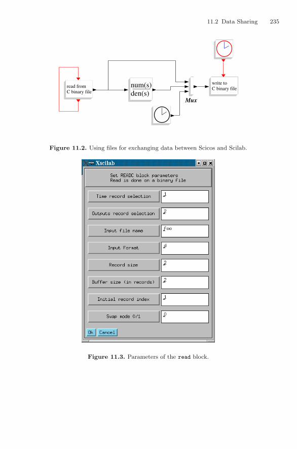
11.2 Data Sharing 235
C binary fileread fromC binary fileread from
den(s)num(s)den(s)num(s)
Mux
C binary filewrite toC binary filewrite to
Figure 11.2. Using files for exchanging data between Scicos and Scilab.
Figure 11.3. Parameters of the read block.
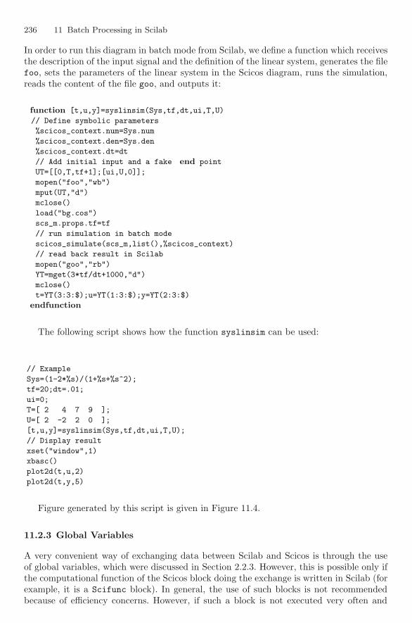
236 11 Batch Processing in Scilab
In order to run this diagram in batch mode from Scilab, we define a function which receivesthe description of the input signal and the definition of the linear system, generates the filefoo, sets the parameters of the linear system in the Scicos diagram, runs the simulation,reads the content of the file goo, and outputs it:
function [t,u,y]=syslinsim(Sys,tf,dt,ui,T,U)
// Define symbolic parameters
%scicos_context.num=Sys.num
%scicos_context.den=Sys.den
%scicos_context.dt=dt
// Add initial input and a fake end point
UT=[[0,T,tf+1];[ui,U,0]];
mopen("foo","wb")
mput(UT,"d")
mclose()
load("bg.cos")
scs_m.props.tf=tf
// run simulation in batch mode
scicos_simulate(scs_m,list(),%scicos_context)
// read back result in Scilab
mopen("goo","rb")
YT=mget(3*tf/dt+1000,"d")
mclose()
t=YT(3:3:$);u=YT(1:3:$);y=YT(2:3:$)
endfunction
The following script shows how the function syslinsim can be used:
// Example
Sys=(1-2*%s)/(1+%s+%s^2);
tf=20;dt=.01;
ui=0;
T=[ 2 4 7 9 ];
U=[ 2 -2 2 0 ];
[t,u,y]=syslinsim(Sys,tf,dt,ui,T,U);
// Display result
xset("window",1)
xbasc()
plot2d(t,u,2)
plot2d(t,y,5)
Figure generated by this script is given in Figure 11.4.
11.2.3 Global Variables
A very convenient way of exchanging data between Scilab and Scicos is through the useof global variables, which were discussed in Section 2.2.3. However, this is possible only ifthe computational function of the Scicos block doing the exchange is written in Scilab (forexample, it is a Scifunc block). In general, the use of such blocks is not recommendedbecause of efficiency concerns. However, if such a block is not executed very often and
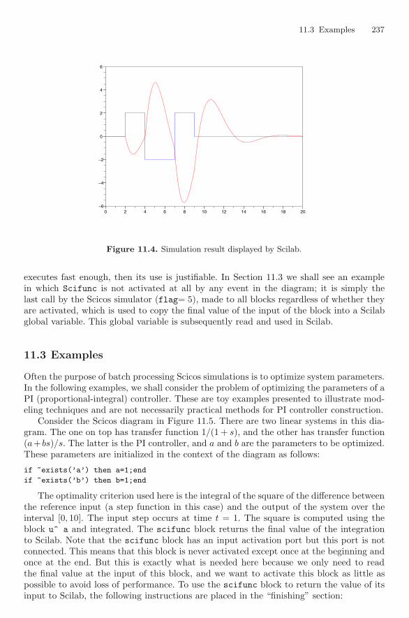
11.3 Examples 237
0 2 4 6 8 10 12 14 16 18 20−6
−4
−2
0
2
4
6
Figure 11.4. Simulation result displayed by Scilab.
executes fast enough, then its use is justifiable. In Section 11.3 we shall see an examplein which Scifunc is not activated at all by any event in the diagram; it is simply thelast call by the Scicos simulator (flag= 5), made to all blocks regardless of whether theyare activated, which is used to copy the final value of the input of the block into a Scilabglobal variable. This global variable is subsequently read and used in Scilab.
11.3 Examples
Often the purpose of batch processing Scicos simulations is to optimize system parameters.In the following examples, we shall consider the problem of optimizing the parameters of aPI (proportional-integral) controller. These are toy examples presented to illustrate mod-eling techniques and are not necessarily practical methods for PI controller construction.
Consider the Scicos diagram in Figure 11.5. There are two linear systems in this dia-gram. The one on top has transfer function 1/(1 + s), and the other has transfer function(a+ bs)/s. The latter is the PI controller, and a and b are the parameters to be optimized.These parameters are initialized in the context of the diagram as follows:
if ~exists(’a’) then a=1;end
if ~exists(’b’) then b=1;end
The optimality criterion used here is the integral of the square of the difference betweenthe reference input (a step function in this case) and the output of the system over theinterval [0, 10]. The input step occurs at time t = 1. The square is computed using theblock u^ a and integrated. The scifunc block returns the final value of the integrationto Scilab. Note that the scifunc block has an input activation port but this port is notconnected. This means that this block is never activated except once at the beginning andonce at the end. But this is exactly what is needed here because we only need to readthe final value at the input of this block, and we want to activate this block as little aspossible to avoid loss of performance. To use the scifunc block to return the value of itsinput to Scilab, the following instructions are placed in the “finishing” section:
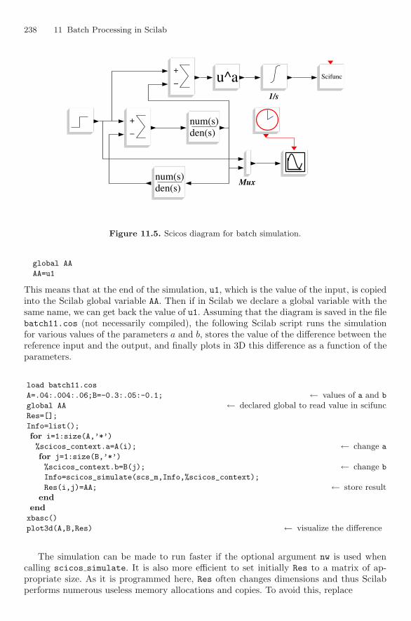
238 11 Batch Processing in Scilab
Mux
den(s)num(s)den(s)num(s)+
−
+
−
den(s)num(s)den(s)num(s)
+
−
+
−
1/s
u^au^a ScifuncScifunc
Figure 11.5. Scicos diagram for batch simulation.
global AA
AA=u1
This means that at the end of the simulation, u1, which is the value of the input, is copiedinto the Scilab global variable AA. Then if in Scilab we declare a global variable with thesame name, we can get back the value of u1. Assuming that the diagram is saved in the filebatch11.cos (not necessarily compiled), the following Scilab script runs the simulationfor various values of the parameters a and b, stores the value of the difference between thereference input and the output, and finally plots in 3D this difference as a function of theparameters.
load batch11.cos
A=.04:.004:.06;B=-0.3:.05:-0.1; ← values of a and b
global AA ← declared global to read value in scifuncRes=[];
Info=list();
for i=1:size(A,’*’)
%scicos_context.a=A(i); ← change a
for j=1:size(B,’*’)
%scicos_context.b=B(j); ← change b
Info=scicos_simulate(scs_m,Info,%scicos_context);
Res(i,j)=AA; ← store resultend
endxbasc()
plot3d(A,B,Res) ← visualize the difference
The simulation can be made to run faster if the optional argument nw is used whencalling scicos simulate. It is also more efficient to set initially Res to a matrix of ap-propriate size. As it is programmed here, Res often changes dimensions and thus Scilabperforms numerous useless memory allocations and copies. To avoid this, replace
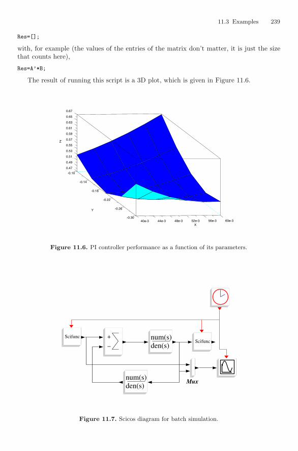
11.3 Examples 239
Res=[];
with, for example (the values of the entries of the matrix don’t matter, it is just the sizethat counts here),
Res=A’*B;
The result of running this script is a 3D plot, which is given in Figure 11.6.
0.47
0.49
0.51
0.53
0.55
0.57
0.59
0.61
0.63
0.65
0.67
Z
40e-3 44e-3 48e-3 52e-3 56e-3 60e-3X
-0.30
-0.26
-0.22
-0.18
-0.14
-0.10
Y
Figure 11.6. PI controller performance as a function of its parameters.
Mux
den(s)num(s)den(s)num(s)+
−
+
−
den(s)num(s)den(s)num(s)
ScifuncScifuncScifuncScifunc
Figure 11.7. Scicos diagram for batch simulation.
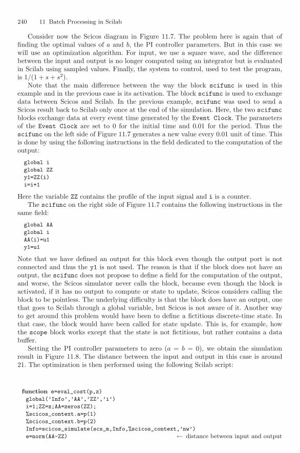
240 11 Batch Processing in Scilab
Consider now the Scicos diagram in Figure 11.7. The problem here is again that offinding the optimal values of a and b, the PI controller parameters. But in this case wewill use an optimization algorithm. For input, we use a square wave, and the differencebetween the input and output is no longer computed using an integrator but is evaluatedin Scilab using sampled values. Finally, the system to control, used to test the program,is 1/(1 + s + s2).
Note that the main difference between the way the block scifunc is used in thisexample and in the previous case is its activation. The block scifunc is used to exchangedata between Scicos and Scilab. In the previous example, scifunc was used to send aScicos result back to Scilab only once at the end of the simulation. Here, the two scifuncblocks exchange data at every event time generated by the Event Clock. The parametersof the Event Clock are set to 0 for the initial time and 0.01 for the period. Thus thescifunc on the left side of Figure 11.7 generates a new value every 0.01 unit of time. Thisis done by using the following instructions in the field dedicated to the computation of theoutput:
global i
global ZZ
y1=ZZ(i)
i=i+1
Here the variable ZZ contains the profile of the input signal and i is a counter.The scifunc on the right side of Figure 11.7 contains the following instructions in the
same field:
global AA
global i
AA(i)=u1
y1=u1
Note that we have defined an output for this block even though the output port is notconnected and thus the y1 is not used. The reason is that if the block does not have anoutput, the scifunc does not propose to define a field for the computation of the output,and worse, the Scicos simulator never calls the block, because even though the block isactivated, if it has no output to compute or state to update, Scicos considers calling theblock to be pointless. The underlying difficulty is that the block does have an output, onethat goes to Scilab through a global variable, but Scicos is not aware of it. Another wayto get around this problem would have been to define a fictitious discrete-time state. Inthat case, the block would have been called for state update. This is, for example, howthe scope block works except that the state is not fictitious, but rather contains a databuffer.
Setting the PI controller parameters to zero (a = b = 0), we obtain the simulationresult in Figure 11.8. The distance between the input and output in this case is around21. The optimization is then performed using the following Scilab script:
function e=eval_cost(p,z)
global(’Info’,’AA’,’ZZ’,’i’)
i=1;ZZ=z;AA=zeros(ZZ);
%scicos_context.a=p(1)
%scicos_context.b=p(2)
Info=scicos_simulate(scs_m,Info,%scicos_context,’nw’)
e=norm(AA-ZZ) ← distance between input and output
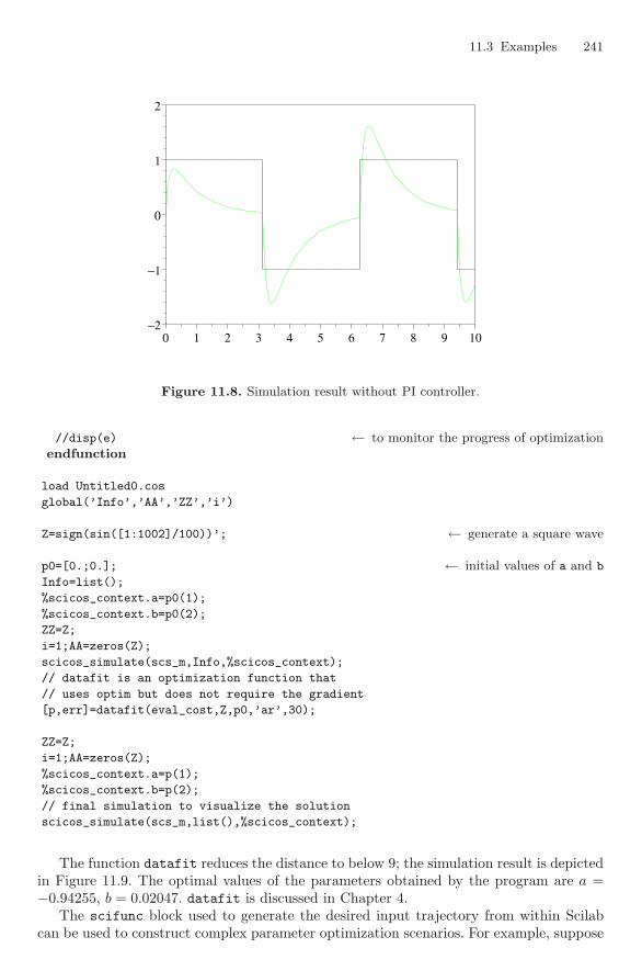
11.3 Examples 241
0 1 2 3 4 5 6 7 8 9 10−2
−1
0
1
2
+
Figure 11.8. Simulation result without PI controller.
//disp(e) ← to monitor the progress of optimizationendfunction
load Untitled0.cos
global(’Info’,’AA’,’ZZ’,’i’)
Z=sign(sin([1:1002]/100))’; ← generate a square wave
p0=[0.;0.]; ← initial values of a and b
Info=list();
%scicos_context.a=p0(1);
%scicos_context.b=p0(2);
ZZ=Z;
i=1;AA=zeros(Z);
scicos_simulate(scs_m,Info,%scicos_context);
// datafit is an optimization function that
// uses optim but does not require the gradient
[p,err]=datafit(eval_cost,Z,p0,’ar’,30);
ZZ=Z;
i=1;AA=zeros(Z);
%scicos_context.a=p(1);
%scicos_context.b=p(2);
// final simulation to visualize the solution
scicos_simulate(scs_m,list(),%scicos_context);
The function datafit reduces the distance to below 9; the simulation result is depictedin Figure 11.9. The optimal values of the parameters obtained by the program are a =−0.94255, b = 0.02047. datafit is discussed in Chapter 4.
The scifunc block used to generate the desired input trajectory from within Scilabcan be used to construct complex parameter optimization scenarios. For example, suppose
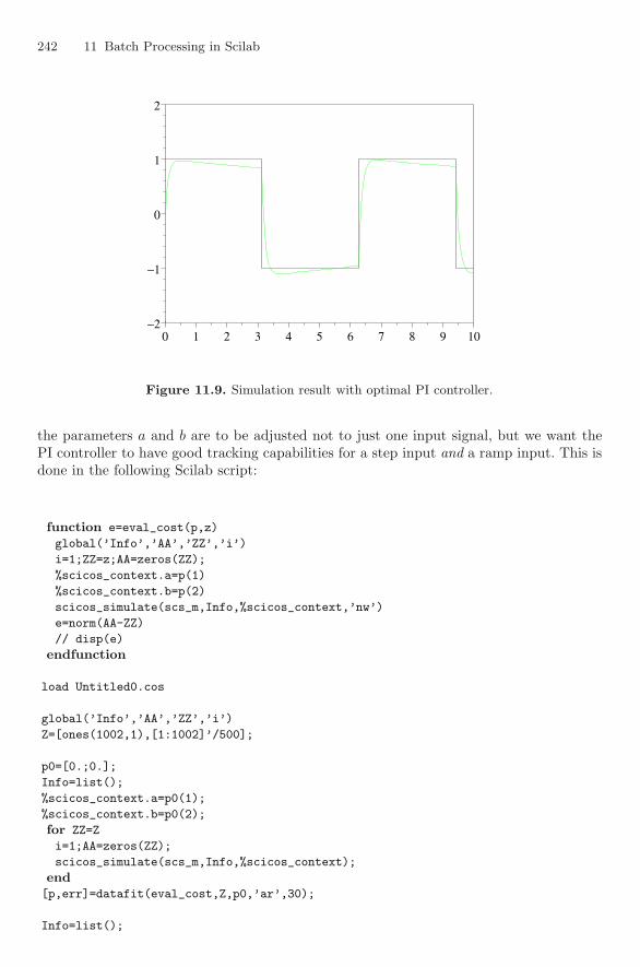
242 11 Batch Processing in Scilab
0 1 2 3 4 5 6 7 8 9 10−2
−1
0
1
2
+
Figure 11.9. Simulation result with optimal PI controller.
the parameters a and b are to be adjusted not to just one input signal, but we want thePI controller to have good tracking capabilities for a step input and a ramp input. This isdone in the following Scilab script:
function e=eval_cost(p,z)
global(’Info’,’AA’,’ZZ’,’i’)
i=1;ZZ=z;AA=zeros(ZZ);
%scicos_context.a=p(1)
%scicos_context.b=p(2)
scicos_simulate(scs_m,Info,%scicos_context,’nw’)
e=norm(AA-ZZ)
// disp(e)
endfunction
load Untitled0.cos
global(’Info’,’AA’,’ZZ’,’i’)
Z=[ones(1002,1),[1:1002]’/500];
p0=[0.;0.];
Info=list();
%scicos_context.a=p0(1);
%scicos_context.b=p0(2);
for ZZ=Z
i=1;AA=zeros(ZZ);
scicos_simulate(scs_m,Info,%scicos_context);
end[p,err]=datafit(eval_cost,Z,p0,’ar’,30);
Info=list();
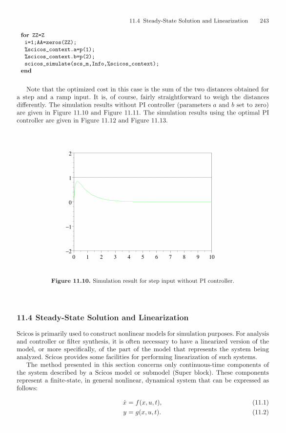
11.4 Steady-State Solution and Linearization 243
for ZZ=Z
i=1;AA=zeros(ZZ);
%scicos_context.a=p(1);
%scicos_context.b=p(2);
scicos_simulate(scs_m,Info,%scicos_context);
end
Note that the optimized cost in this case is the sum of the two distances obtained fora step and a ramp input. It is, of course, fairly straightforward to weigh the distancesdifferently. The simulation results without PI controller (parameters a and b set to zero)are given in Figure 11.10 and Figure 11.11. The simulation results using the optimal PIcontroller are given in Figure 11.12 and Figure 11.13.
0 1 2 3 4 5 6 7 8 9 10−2
−1
0
1
2
+
Figure 11.10. Simulation result for step input without PI controller.
11.4 Steady-State Solution and Linearization
Scicos is primarily used to construct nonlinear models for simulation purposes. For analysisand controller or filter synthesis, it is often necessary to have a linearized version of themodel, or more specifically, of the part of the model that represents the system beinganalyzed. Scicos provides some facilities for performing linearization of such systems.
The method presented in this section concerns only continuous-time components ofthe system described by a Scicos model or submodel (Super block). These componentsrepresent a finite-state, in general nonlinear, dynamical system that can be expressed asfollows:
x = f(x, u, t), (11.1)y = g(x, u, t). (11.2)
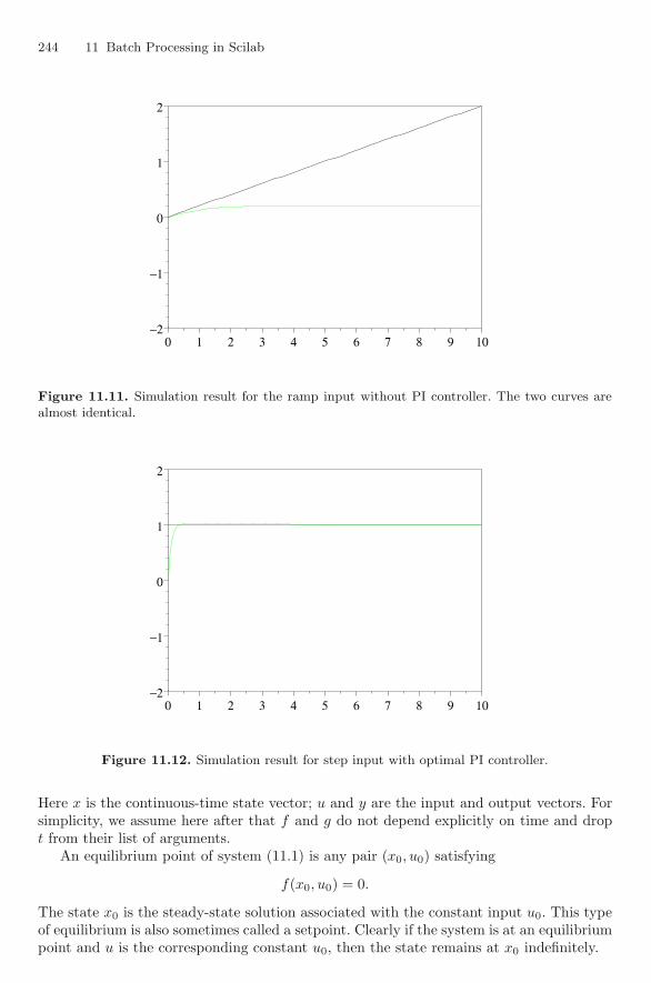
244 11 Batch Processing in Scilab
0 1 2 3 4 5 6 7 8 9 10−2
−1
0
1
2
+
Figure 11.11. Simulation result for the ramp input without PI controller. The two curves arealmost identical.
0 1 2 3 4 5 6 7 8 9 10−2
−1
0
1
2
+
Figure 11.12. Simulation result for step input with optimal PI controller.
Here x is the continuous-time state vector; u and y are the input and output vectors. Forsimplicity, we assume here after that f and g do not depend explicitly on time and dropt from their list of arguments.
An equilibrium point of system (11.1) is any pair (x0, u0) satisfying
f(x0, u0) = 0.
The state x0 is the steady-state solution associated with the constant input u0. This typeof equilibrium is also sometimes called a setpoint. Clearly if the system is at an equilibriumpoint and u is the corresponding constant u0, then the state remains at x0 indefinitely.
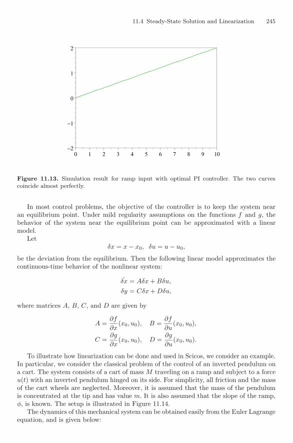
11.4 Steady-State Solution and Linearization 245
0 1 2 3 4 5 6 7 8 9 10−2
−1
0
1
2
+
Figure 11.13. Simulation result for ramp input with optimal PI controller. The two curvescoincide almost perfectly.
In most control problems, the objective of the controller is to keep the system nearan equilibrium point. Under mild regularity assumptions on the functions f and g, thebehavior of the system near the equilibrium point can be approximated with a linearmodel.
Letδx = x − x0, δu = u − u0,
be the deviation from the equilibrium. Then the following linear model approximates thecontinuous-time behavior of the nonlinear system:
˙δx = Aδx + Bδu,
δy = Cδx + Dδu,
where matrices A, B, C, and D are given by
A =∂f
∂x(x0, u0), B =
∂f
∂u(x0, u0),
C =∂g
∂x(x0, u0), D =
∂g
∂u(x0, u0).
To illustrate how linearization can be done and used in Scicos, we consider an example.In particular, we consider the classical problem of the control of an inverted pendulum ona cart. The system consists of a cart of mass M traveling on a ramp and subject to a forceu(t) with an inverted pendulum hinged on its side. For simplicity, all friction and the massof the cart wheels are neglected. Moreover, it is assumed that the mass of the pendulumis concentrated at the tip and has value m. It is also assumed that the slope of the ramp,φ, is known. The setup is illustrated in Figure 11.14.
The dynamics of this mechanical system can be obtained easily from the Euler Lagrangeequation, and is given below:
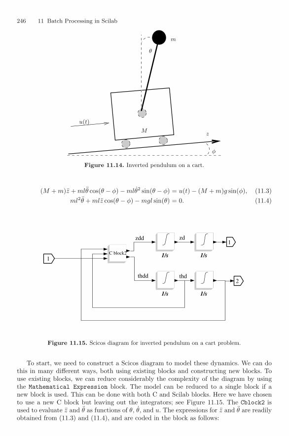
246 11 Batch Processing in Scilab
φ
θ
u(t)
z
m
M
Figure 11.14. Inverted pendulum on a cart.
(M + m)z + mlθ cos(θ − φ) − mlθ2 sin(θ − φ) = u(t) − (M + m)g sin(φ), (11.3)ml2θ + mlz cos(θ − φ) − mgl sin(θ) = 0. (11.4)
C block2C block2 1/s 1/s
1/s 1/s
zdd
thdd
zd
thd
11
11
22
Figure 11.15. Scicos diagram for inverted pendulum on a cart problem.
To start, we need to construct a Scicos diagram to model these dynamics. We can dothis in many different ways, both using existing blocks and constructing new blocks. Touse existing blocks, we can reduce considerably the complexity of the diagram by usingthe Mathematical Expression block. The model can be reduced to a single block if anew block is used. This can be done with both C and Scilab blocks. Here we have chosento use a new C block but leaving out the integrators; see Figure 11.15. The Cblock2 isused to evaluate z and θ as functions of θ, θ, and u. The expressions for z and θ are readilyobtained from (11.3) and (11.4), and are coded in the block as follows:
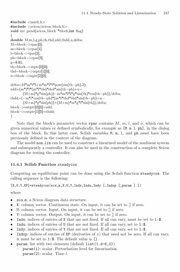
11.4 Steady-State Solution and Linearization 247
#include <math.h>#include <scicos/scicos block.h>void inv pend(scicos block *block,int flag){double M,m,l,g,ph,th,thd,zdd,thdd,u,delta;M=block−>rpar[0];m=block−>rpar[1];l=block−>rpar[2];ph=block−>rpar[3];g=9.81;th=block−>inptr[0][0];thd=block−>inptr[1][0];u=block−>inptr[2][0];
delta=M*m*l*l+m*m*l*l*pow(sin(th−ph),2);zdd=(m*l*l*(m*l*thd*thd*sin(th−ph)+u−
(M+m)*g*sin(ph))−m*m*l*l*g*sin(th)*cos(th−ph))/delta;thdd=(−m*l*cos(th−ph)*(m*l*thd*thd*sin(th−ph)+u−
(M+m)*g*sin(ph))+(M+m)*m*g*l*sin(th))/delta;block−>outptr[0][0]=zdd;block−>outptr[1][0]=thdd;}
Note that the block’s parameter vector rpar contains M , m, l, and φ, which can begiven numerical values or defined symbolically, for example as [M m l ph], in the dialogbox of the block. In this latter case, Scilab variables M, m, l, and ph must have beenpreviously defined in the context of the diagram.
The model non lin can be used to construct a linearized model of the nonlinear systemand subsequently a controller. It can also be used in the construction of a complete Scicosdiagram for testing the controller.
11.4.1 Scilab Function steadycos
Computing an equilibrium point can be done using the Scilab function steadycos. Thecalling sequence is the following:
[X,U,Y,XP]=steadycos(scs_m,X,U,Y,Indx,Indu,Indy [,Indxp [,param ] ])
where
• scs m: a Scicos diagram data structure.• X: column vector. Continuous state. On input, it can be set to [] if zero.• U: column vector. Input. On input, it can be set to [] if zero.• Y: column vector. Output. On input, it can be set to [] if zero.• Indx: indices of entries of X that are not fixed. If all can vary, must be set to 1:$.• Indu: indices of entries of U that are not fixed. If all can vary, set to 1:$.• Indy: indices of entries of Y that are not fixed. If all can vary, set to 1:$.• Indxp: indices of entries of XP (derivative of x) that need not be zero. If all can vary,
it must be set to 1:$. The default value is [].• param: list with two elements (default list(1.d-6,0))
– param(1): scalar. Perturbation level for linearization.– param(2): scalar. Time t.
248 11 Batch Processing in Scilab
The equilibrium point is, in general, not unique, and parts of the vectors x0 and u0
can be set a priori to desired values. Vector indices are used to specify parts of the stateand the input that are free to be adjusted by the program. Even by specifying properlythese indices, the equilibrium point may not be unique and the input arguments X and Ucan be used to direct the search toward a desired solution since they are used as initialguess values for the search algorithm.
Often the problem of finding an equilibrium point is that of finding a steady-statesolution for a given input, in which case Indu is set to [] and Indx to 1:$. But in theexample we are considering in this section, the equilibrium point we are looking for hasan unknown u0 and a known x0. The desired objective is to keep the cart at the centerwith the pendulum pointing upward. The force u0 is what is needed to prevent the cartfrom moving; that is, it compensates for the force of gravity. It is not difficult to see that
u0 = (M + m)g sin(φ), (11.5)
but we let the program find this by itself. This is done using the following commands:
�−→ load non_lin.cos
�−→ [X,U,Y,XP]=steadycos(scs_m,[],[],[],[],1,1:$)
XP =
1.0E-16 *
! 0.3830958 !
! 0. !
! - 0.3811819 !
! 0. !
Y =
! 0. !
! 0. !
U =
12.731756
X =
! 0. !
! 0. !
! 0. !
! 0. !
Here it is assumed that the Scicos diagram non lin has been saved in the current directory.Loading non lin.cos provides the variable scs m, which contains all the informa-
tion regarding the diagram. This variable is then used as the argument to the functionsteadycos.
11.4.2 Scilab Function lincos
Computing the linearized system around an equilibrium point can be done using the Scilabfunction lincos. The calling sequence is the following:
sys= lincos(scs_m [,x0,u0 [,param] ])
where
• scs m: a Scicos diagram data structure.• x0: column vector. Continuous-time state around which linearization is to be done
(default value is 0).• u0: column vector. Input around which linearization is to be done (default is 0).
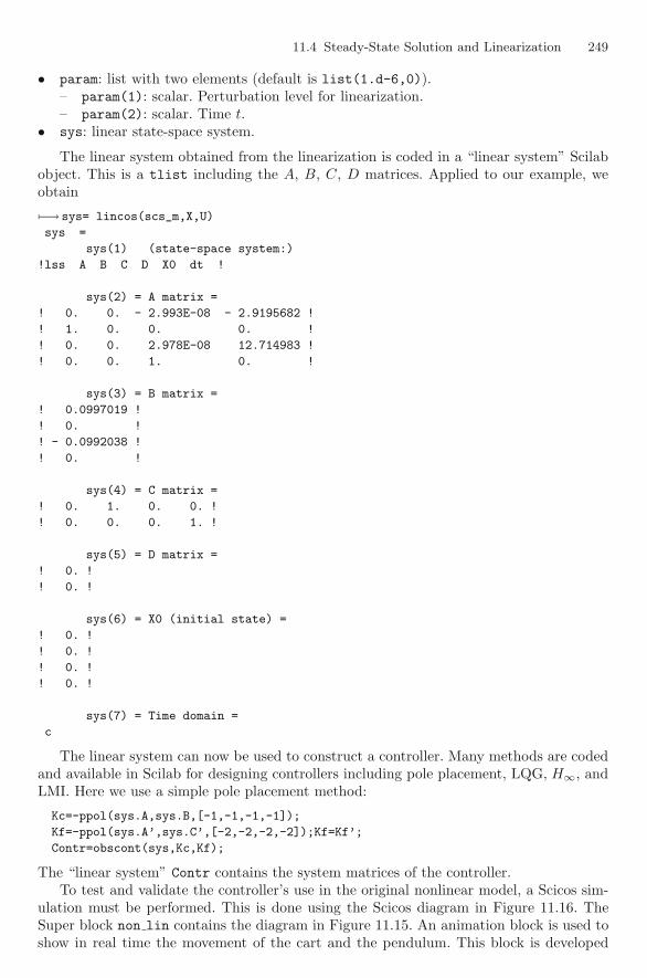
11.4 Steady-State Solution and Linearization 249
• param: list with two elements (default is list(1.d-6,0)).– param(1): scalar. Perturbation level for linearization.– param(2): scalar. Time t.
• sys: linear state-space system.
The linear system obtained from the linearization is coded in a “linear system” Scilabobject. This is a tlist including the A, B, C, D matrices. Applied to our example, weobtain
�−→ sys= lincos(scs_m,X,U)
sys =
sys(1) (state-space system:)
!lss A B C D X0 dt !
sys(2) = A matrix =
! 0. 0. - 2.993E-08 - 2.9195682 !
! 1. 0. 0. 0. !
! 0. 0. 2.978E-08 12.714983 !
! 0. 0. 1. 0. !
sys(3) = B matrix =
! 0.0997019 !
! 0. !
! - 0.0992038 !
! 0. !
sys(4) = C matrix =
! 0. 1. 0. 0. !
! 0. 0. 0. 1. !
sys(5) = D matrix =
! 0. !
! 0. !
sys(6) = X0 (initial state) =
! 0. !
! 0. !
! 0. !
! 0. !
sys(7) = Time domain =
c
The linear system can now be used to construct a controller. Many methods are codedand available in Scilab for designing controllers including pole placement, LQG, H∞, andLMI. Here we use a simple pole placement method:
Kc=-ppol(sys.A,sys.B,[-1,-1,-1,-1]);
Kf=-ppol(sys.A’,sys.C’,[-2,-2,-2,-2]);Kf=Kf’;
Contr=obscont(sys,Kc,Kf);
The “linear system” Contr contains the system matrices of the controller.To test and validate the controller’s use in the original nonlinear model, a Scicos sim-
ulation must be performed. This is done using the Scicos diagram in Figure 11.16. TheSuper block non lin contains the diagram in Figure 11.15. An animation block is used toshow in real time the movement of the cart and the pendulum. This block is developed
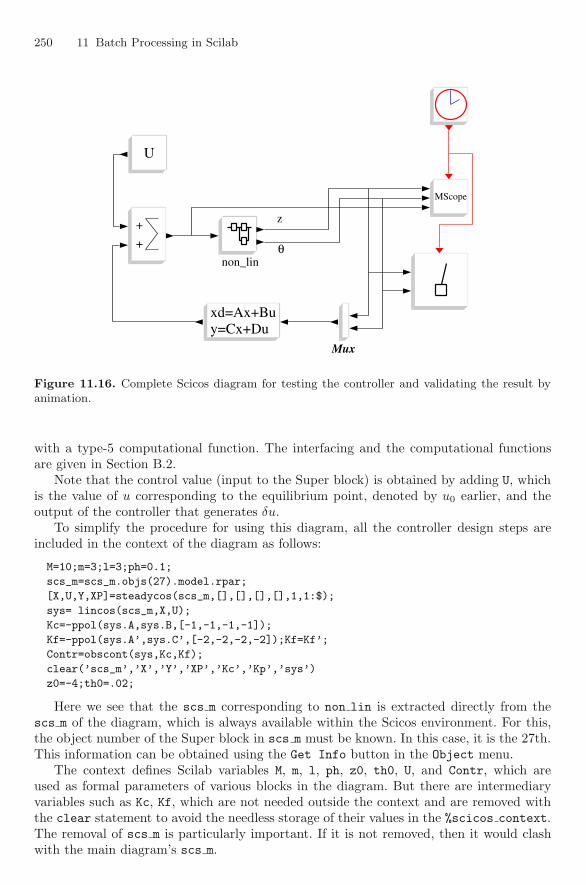
250 11 Batch Processing in Scilab
U U
MScopeMScope
y=Cx+Duxd=Ax+Buy=Cx+Duxd=Ax+Bu
Mux
+
+
+
+
non_lin
z
θ
Figure 11.16. Complete Scicos diagram for testing the controller and validating the result byanimation.
with a type-5 computational function. The interfacing and the computational functionsare given in Section B.2.
Note that the control value (input to the Super block) is obtained by adding U, whichis the value of u corresponding to the equilibrium point, denoted by u0 earlier, and theoutput of the controller that generates δu.
To simplify the procedure for using this diagram, all the controller design steps areincluded in the context of the diagram as follows:
M=10;m=3;l=3;ph=0.1;
scs_m=scs_m.objs(27).model.rpar;
[X,U,Y,XP]=steadycos(scs_m,[],[],[],[],1,1:$);
sys= lincos(scs_m,X,U);
Kc=-ppol(sys.A,sys.B,[-1,-1,-1,-1]);
Kf=-ppol(sys.A’,sys.C’,[-2,-2,-2,-2]);Kf=Kf’;
Contr=obscont(sys,Kc,Kf);
clear(’scs_m’,’X’,’Y’,’XP’,’Kc’,’Kp’,’sys’)
z0=-4;th0=.02;
Here we see that the scs m corresponding to non lin is extracted directly from thescs m of the diagram, which is always available within the Scicos environment. For this,the object number of the Super block in scs m must be known. In this case, it is the 27th.This information can be obtained using the Get Info button in the Object menu.
The context defines Scilab variables M, m, l, ph, z0, th0, U, and Contr, which areused as formal parameters of various blocks in the diagram. But there are intermediaryvariables such as Kc, Kf, which are not needed outside the context and are removed withthe clear statement to avoid the needless storage of their values in the %scicos context.The removal of scs m is particularly important. If it is not removed, then it would clashwith the main diagram’s scs m.
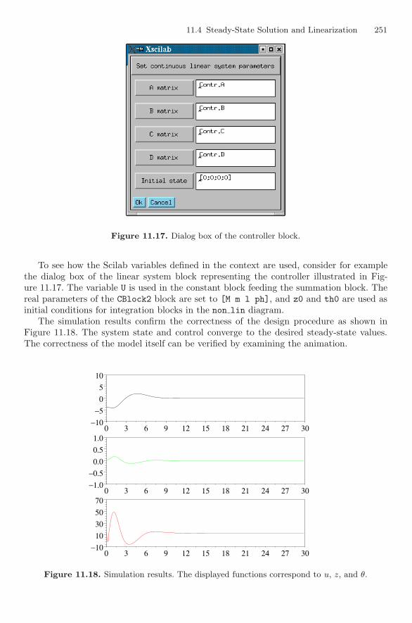
11.4 Steady-State Solution and Linearization 251
Figure 11.17. Dialog box of the controller block.
To see how the Scilab variables defined in the context are used, consider for examplethe dialog box of the linear system block representing the controller illustrated in Fig-ure 11.17. The variable U is used in the constant block feeding the summation block. Thereal parameters of the CBlock2 block are set to [M m l ph], and z0 and th0 are used asinitial conditions for integration blocks in the non lin diagram.
The simulation results confirm the correctness of the design procedure as shown inFigure 11.18. The system state and control converge to the desired steady-state values.The correctness of the model itself can be verified by examining the animation.
0 3 6 9 12 15 18 21 24 27 30−10
−505
10
+
0 3 6 9 12 15 18 21 24 27 30−1.0−0.5
0.00.51.0
+
0 3 6 9 12 15 18 21 24 27 30−10
10305070
+
Figure 11.18. Simulation results. The displayed functions correspond to u, z, and θ.
12
Code Generation
Scicos provides a code-generation facility that can be used to create C code for a modeldefined in Scicos. Code generation has many applications. It can be used to improvesimulation performance. Even though Scicos diagrams are compiled in the sense that allthe scheduling tables are precomputed, there is still some overhead in using the Scicossimulator that is eliminated by running the code that has been generated. Even if theperformance gain is not significant, replacing a Super block with a basic block may be ofinterest if the designer of the model does not want to reveal the content of the Super block.If the Super block is converted to a basic block, the designer can then simply distributea compiled version of the generated code. But the most important application of codegeneration is the creation of standalone applications (programs that run independently ofScilab), which can be used, in particular, in real-time applications.
This chapter discusses how the code-generation facility can be used and what thelimitations are. Some examples are provided.
12.1 Code Generation Procedure
The Code Generation item in the Object menu can be used to generate C code forthe submodel defined within a Super block. In addition, once invoked, Code Generationcompiles and links incrementally the generated code with Scilab and replaces the Superblock with a basic block having for computational function the generated code. Exceptin some special situations that we shall discuss later, the replacement of the Super blockwith this new block should not alter simulation results in any way. Code Generation alsocreates a main C program implementing a standalone application.
Consider the Scicos diagram in Figure 12.1. In this model, a random number is gener-ated by the random generator block at every clock event. The block parameter is set sothat the random number can be both positive and negative. If the number is positive, theIf-then-else block activates the memory block 1/z, which is updated by adding its pre-vious value to the (positive) value of the random number. Finally, the result is displayedin the scope alongside the values of the random signal.
The simulation result shows, as expected, that the output of the memory block increasesonly when the random number is positive. The output remains constant otherwise. SeeFigure 12.2.
Suppose now that we want to isolate the part of the diagram that receives a numberand, depending on its sign, adds it to a counter, in order to perform code generation for
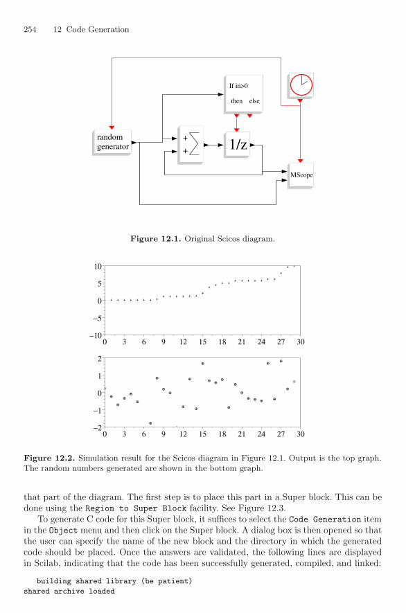
254 12 Code Generation
generatorrandomgeneratorrandom
MScopeMScope
1/z1/z
then else
If in>0
then else
If in>0
+
+
+
+
Figure 12.1. Original Scicos diagram.
0 3 6 9 12 15 18 21 24 27 30−10
−5
0
5
10
+
0 3 6 9 12 15 18 21 24 27 30−2
−1
0
1
2
+
+ +
⊕
⊕
+ +
⊕
⊕
+ +
⊕
⊕
+ +
⊕⊕
+ +
⊕
⊕
+ +
⊕
+ +
⊕
+ +
⊕
⊕
++
⊕
⊕
+ +
⊕⊕
+ +
⊕
⊕
+ +
⊕
⊕
+ +
⊕
⊕
+ +
⊕
⊕
++
⊕
⊕
+
+
⊕
⊕
++
⊕ ⊕
+ +
⊕⊕
+ +
⊕
⊕
++
⊕
⊕
+ +
⊕
⊕
+ +
⊕
⊕
+ +
⊕ ⊕
+ +
⊕ ⊕
+ +
⊕
⊕
+ +
⊕
⊕
+
+
⊕
⊕
+
+
⊕
⊕
+ +
⊕
⊕
Figure 12.2. Simulation result for the Scicos diagram in Figure 12.1. Output is the top graph.The random numbers generated are shown in the bottom graph.
that part of the diagram. The first step is to place this part in a Super block. This can bedone using the Region to Super Block facility. See Figure 12.3.
To generate C code for this Super block, it suffices to select the Code Generation itemin the Object menu and then click on the Super block. A dialog box is then opened so thatthe user can specify the name of the new block and the directory in which the generatedcode should be placed. Once the answers are validated, the following lines are displayedin Scilab, indicating that the code has been successfully generated, compiled, and linked:
building shared library (be patient)
shared archive loaded

12.1 Code Generation Procedure 255
generatorrandomgeneratorrandom
MScopeMScope
Figure 12.3. Scicos diagram in Figure 12.1 after isolating the part for which code generation isto be done.
Link done
Link done
Subsequently, the Super block is converted into a block; see Figure 12.4. Simulation canbe performed to verify that this operation has not altered system behavior.
generatorrandomgeneratorrandom
MScopeMScope
ExampleExample
Figure 12.4. Scicos diagram after code generation.
This code generation operation creates a number of files in the specified directory.Since we have named our new block Example, all of the generated file names start withExample. The main file is Example.c, which is the computational function of the new
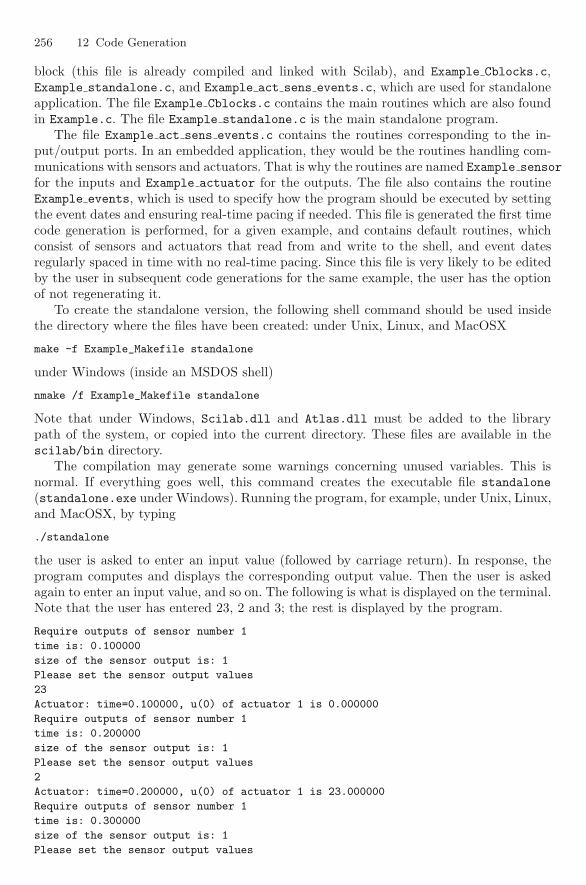
256 12 Code Generation
block (this file is already compiled and linked with Scilab), and Example Cblocks.c,Example standalone.c, and Example act sens events.c, which are used for standaloneapplication. The file Example Cblocks.c contains the main routines which are also foundin Example.c. The file Example standalone.c is the main standalone program.
The file Example act sens events.c contains the routines corresponding to the in-put/output ports. In an embedded application, they would be the routines handling com-munications with sensors and actuators. That is why the routines are named Example sensorfor the inputs and Example actuator for the outputs. The file also contains the routineExample events, which is used to specify how the program should be executed by settingthe event dates and ensuring real-time pacing if needed. This file is generated the first timecode generation is performed, for a given example, and contains default routines, whichconsist of sensors and actuators that read from and write to the shell, and event datesregularly spaced in time with no real-time pacing. Since this file is very likely to be editedby the user in subsequent code generations for the same example, the user has the optionof not regenerating it.
To create the standalone version, the following shell command should be used insidethe directory where the files have been created: under Unix, Linux, and MacOSX
make -f Example_Makefile standalone
under Windows (inside an MSDOS shell)
nmake /f Example_Makefile standalone
Note that under Windows, Scilab.dll and Atlas.dll must be added to the librarypath of the system, or copied into the current directory. These files are available in thescilab/bin directory.
The compilation may generate some warnings concerning unused variables. This isnormal. If everything goes well, this command creates the executable file standalone(standalone.exe under Windows). Running the program, for example, under Unix, Linux,and MacOSX, by typing
./standalone
the user is asked to enter an input value (followed by carriage return). In response, theprogram computes and displays the corresponding output value. Then the user is askedagain to enter an input value, and so on. The following is what is displayed on the terminal.Note that the user has entered 23, 2 and 3; the rest is displayed by the program.
Require outputs of sensor number 1
time is: 0.100000
size of the sensor output is: 1
Please set the sensor output values
23
Actuator: time=0.100000, u(0) of actuator 1 is 0.000000
Require outputs of sensor number 1
time is: 0.200000
size of the sensor output is: 1
Please set the sensor output values
2
Actuator: time=0.200000, u(0) of actuator 1 is 23.000000
Require outputs of sensor number 1
time is: 0.300000
size of the sensor output is: 1
Please set the sensor output values
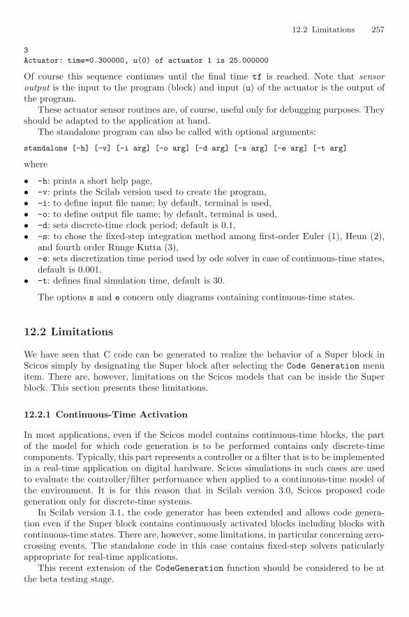
12.2 Limitations 257
3
Actuator: time=0.300000, u(0) of actuator 1 is 25.000000
Of course this sequence continues until the final time tf is reached. Note that sensoroutput is the input to the program (block) and input (u) of the actuator is the output ofthe program.
These actuator sensor routines are, of course, useful only for debugging purposes. Theyshould be adapted to the application at hand.
The standalone program can also be called with optional arguments:
standalone [-h] [-v] [-i arg] [-o arg] [-d arg] [-s arg] [-e arg] [-t arg]
where
• -h: prints a short help page,• -v: prints the Scilab version used to create the program,• -i: to define input file name; by default, terminal is used,• -o: to define output file name; by default, terminal is used,• -d: sets discrete-time clock period; default is 0.1,• -s: to chose the fixed-step integration method among first-order Euler (1), Heun (2),
and fourth order Runge Kutta (3),• -e: sets discretization time period used by ode solver in case of continuous-time states,
default is 0.001,• -t: defines final simulation time, default is 30.
The options s and e concern only diagrams containing continuous-time states.
12.2 Limitations
We have seen that C code can be generated to realize the behavior of a Super block inScicos simply by designating the Super block after selecting the Code Generation menuitem. There are, however, limitations on the Scicos models that can be inside the Superblock. This section presents these limitations.
12.2.1 Continuous-Time Activation
In most applications, even if the Scicos model contains continuous-time blocks, the partof the model for which code generation is to be performed contains only discrete-timecomponents. Typically, this part represents a controller or a filter that is to be implementedin a real-time application on digital hardware. Scicos simulations in such cases are usedto evaluate the controller/filter performance when applied to a continuous-time model ofthe environment. It is for this reason that in Scilab version 3.0, Scicos proposed codegeneration only for discrete-time systems.
In Scilab version 3.1, the code generator has been extended and allows code genera-tion even if the Super block contains continuously activated blocks including blocks withcontinuous-time states. There are, however, some limitations, in particular concerning zero-crossing events. The standalone code in this case contains fixed-step solvers paticularlyappropriate for real-time applications.
This recent extension of the CodeGeneration function should be considered to be atthe beta testing stage.

258 12 Code Generation
12.2.2 Synchronicism
We have seen that code generation is done by first converting the Super block for whichcode generation is done into a basic block. This is done, in particular, for testing thegenerated code. But we have also seen that a basic Scicos block cannot be self activated.Its activation must come from the outside. This sets some limitations on the class of Superblocks that can be handled by Code Generation. Consider the Super block model depictedin Figure 12.5.
1111 1/z1/z S/HS/H
DelayEventDelayEvent
11
Figure 12.5. Asynchronous Super block diagram.
In this example, the 1/z and the S/H blocks are not synchronous. The reason is thatS/H is activated by the output of the Event Delay block and the events correspondingto this output are not synchronous with the input events of this block that activate the1/z block. In fact, no Scicos basic block can produce output events synchronous with itsinput events, the only exceptions being the If-then-else and event select block,s which,strictly speaking, are not blocks. So a hard constraint on the blocks within the Super blockis that none should have an output activation port unless it is an If-then-else or anevent select block.
12.3 A Look Inside
Code generation is done by the Scilab function CodeGeneration , which can be found inthe directory scilab/macros/scicos. This function takes a Scicos model (model insidethe designated Super block) and converts it into a regular block by generating the cor-responding computational function in the C language. It also generates a standalone Cprogram. The code generation is done in five steps: diagram construction, compilation,code generation, block construction, and substitution.
Diagram Construction
The subdiagram within the designated Super block is extracted and used to construct anew Scicos diagram. This requires modifying the subdiagram because of the presence ofinput/output ports that are not Scicos blocks. These ports, used inside Super blocks, areeliminated at a precompilation stage when the original diagram is compiled.
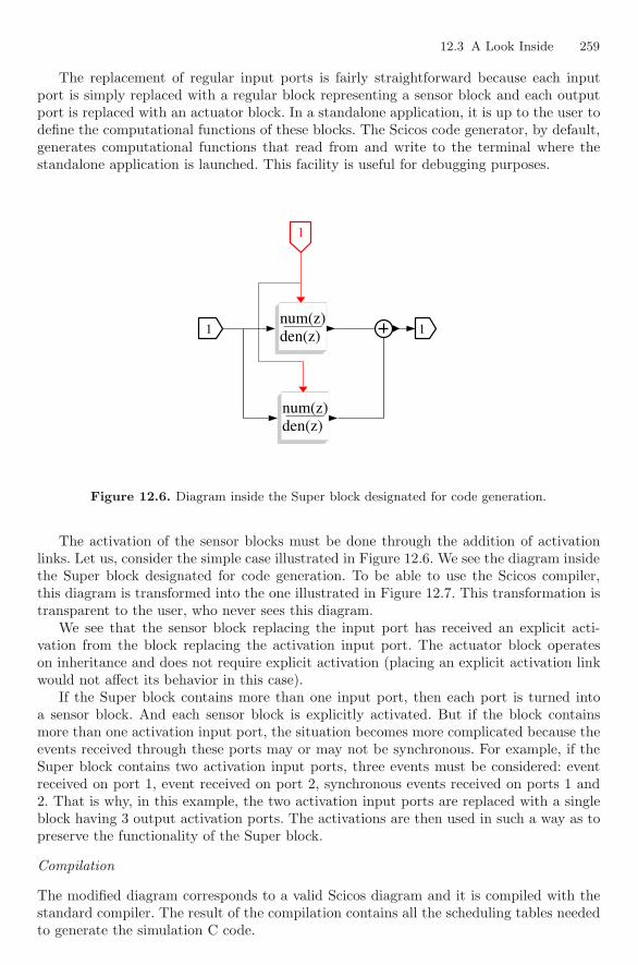
12.3 A Look Inside 259
The replacement of regular input ports is fairly straightforward because each inputport is simply replaced with a regular block representing a sensor block and each outputport is replaced with an actuator block. In a standalone application, it is up to the user todefine the computational functions of these blocks. The Scicos code generator, by default,generates computational functions that read from and write to the terminal where thestandalone application is launched. This facility is useful for debugging purposes.
den(z)num(z)den(z)num(z)
den(z)num(z)den(z)num(z)
11
11
11
Figure 12.6. Diagram inside the Super block designated for code generation.
The activation of the sensor blocks must be done through the addition of activationlinks. Let us, consider the simple case illustrated in Figure 12.6. We see the diagram insidethe Super block designated for code generation. To be able to use the Scicos compiler,this diagram is transformed into the one illustrated in Figure 12.7. This transformation istransparent to the user, who never sees this diagram.
We see that the sensor block replacing the input port has received an explicit acti-vation from the block replacing the activation input port. The actuator block operateson inheritance and does not require explicit activation (placing an explicit activation linkwould not affect its behavior in this case).
If the Super block contains more than one input port, then each port is turned intoa sensor block. And each sensor block is explicitly activated. But if the block containsmore than one activation input port, the situation becomes more complicated because theevents received through these ports may or may not be synchronous. For example, if theSuper block contains two activation input ports, three events must be considered: eventreceived on port 1, event received on port 2, synchronous events received on ports 1 and2. That is why, in this example, the two activation input ports are replaced with a singleblock having 3 output activation ports. The activations are then used in such a way as topreserve the functionality of the Super block.
Compilation
The modified diagram corresponds to a valid Scicos diagram and it is compiled with thestandard compiler. The result of the compilation contains all the scheduling tables neededto generate the simulation C code.
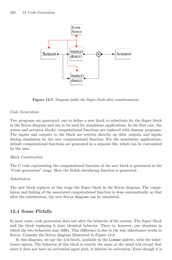
260 12 Code Generation
den(z)num(z)den(z)num(z)
den(z)num(z)den(z)num(z)
SensorSensor
SourceEventSourceEvent
ActuatorActuator
Figure 12.7. Diagram inside the Super block after transformation.
Code Generation
Two programs are generated: one to define a new block to substitute for the Super blockin the Scicos diagram and one to be used for standalone applications. In the first case, thesensor and actuator blocks’ computational functions are replaced with dummy programs.The inputs and outputs to the block are written directly on their outputs and inputsduring simulation by the new computational function. For the standalone applications,default computational functions are generated in a separate file, which can be customizedby the user.
Block Construction
The C code representing the computational function of the new block is generated at the“Code generation” stage. Here the Scilab interfacing function is generated.
Substitution
The new block replaces at this stage the Super block in the Scicos diagram. The compi-lation and linking of the associated computational function is done automatically so thatafter the substitution, the new Scicos diagram can be simulated.
12.4 Some Pitfalls
In most cases, code generation does not alter the behavior of the system. The Super blockand the block replacing it have identical behavior. There is, however, one situation inwhich the two behaviors may differ. This difference is due to the way inheritance works inScicos. Consider the Scicos diagram illustrated in Figure 12.8.
In this diagram, we use the 1/z block, available in the Linear palette, with the inher-itance option. The behavior of this block is exactly the same as the usual 1/z except thatsince it does not have an activation input port, it inherits its activation. Even though it is
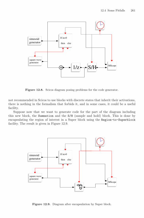
12.4 Some Pitfalls 261
MScopeMScopegeneratorsquare wavegeneratorsquare wave
then else
If in>0
then else
If in>0
1/z1/z S/HS/H
generatorsinusoidgeneratorsinusoid
Figure 12.8. Scicos diagram posing problems for the code generator.
not recommended in Scicos to use blocks with discrete states that inherit their activations,there is nothing in the formalism that forbids it, and in some cases, it could be a usefulfacility.
Suppose now that we want to generate code for the part of the diagram includingthis new block, the Summation and the S/H (sample and hold) block. This is done byencapsulating the region of interest in a Super block using the Region-to-Superblockfacility. The result is given in Figure 12.9.
MScopeMScopegeneratorsquare wavegeneratorsquare wave
then else
If in>0
then else
If in>0
generatorsinusoidgeneratorsinusoid
Figure 12.9. Diagram after encapsulation by Super block.
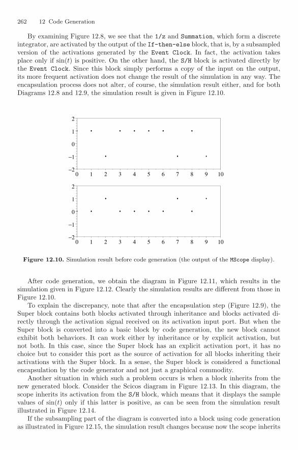
262 12 Code Generation
By examining Figure 12.8, we see that the 1/z and Summation, which form a discreteintegrator, are activated by the output of the If-then-else block, that is, by a subsampledversion of the activations generated by the Event Clock. In fact, the activation takesplace only if sin(t) is positive. On the other hand, the S/H block is activated directly bythe Event Clock. Since this block simply performs a copy of the input on the output,its more frequent activation does not change the result of the simulation in any way. Theencapsulation process does not alter, of course, the simulation result either, and for bothDiagrams 12.8 and 12.9, the simulation result is given in Figure 12.10.
0 1 2 3 4 5 6 7 8 9 10−2
−1
0
1
2
+
0 1 2 3 4 5 6 7 8 9 10−2
−1
0
1
2
+
♦ ♦
♦ ♦
♦
♦
♦
♦
♦
♦
♦
♦
♦ ♦
♦ ♦
♦ ♦
♦ ♦
♦ ♦
♦ ♦
♦
♦
♦
♦
♦
♦
♦
♦
♦
♦
♦
♦
Figure 12.10. Simulation result before code generation (the output of the MScope display).
After code generation, we obtain the diagram in Figure 12.11, which results in thesimulation given in Figure 12.12. Clearly the simulation results are different from those inFigure 12.10.
To explain the discrepancy, note that after the encapsulation step (Figure 12.9), theSuper block contains both blocks activated through inheritance and blocks activated di-rectly through the activation signal received on its activation input port. But when theSuper block is converted into a basic block by code generation, the new block cannotexhibit both behaviors. It can work either by inheritance or by explicit activation, butnot both. In this case, since the Super block has an explicit activation port, it has nochoice but to consider this port as the source of activation for all blocks inheriting theiractivations with the Super block. In a sense, the Super block is considered a functionalencapsulation by the code generator and not just a graphical commodity.
Another situation in which such a problem occurs is when a block inherits from thenew generated block. Consider the Scicos diagram in Figure 12.13. In this diagram, thescope inherits its activation from the S/H block, which means that it displays the samplevalues of sin(t) only if this latter is positive, as can be seen from the simulation resultillustrated in Figure 12.14.
If the subsampling part of the diagram is converted into a block using code generationas illustrated in Figure 12.15, the simulation result changes because now the scope inherits
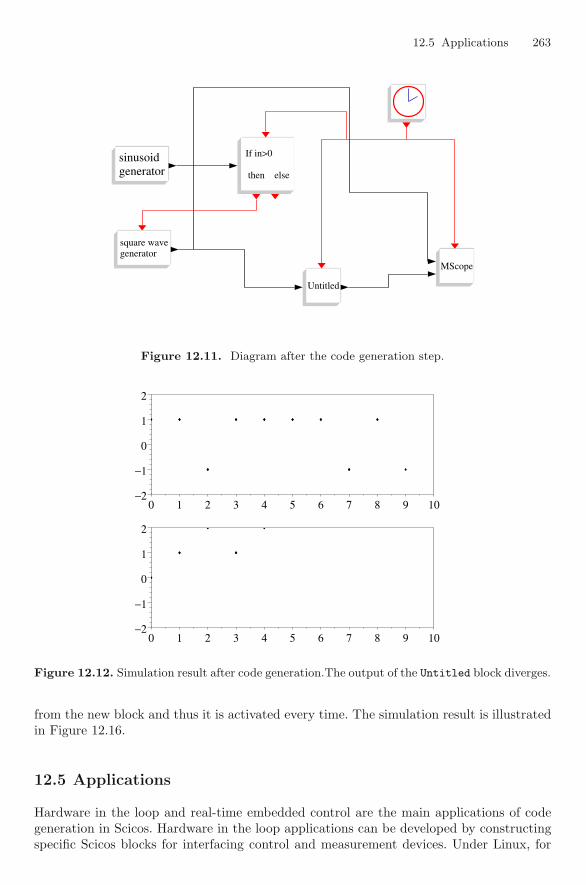
12.5 Applications 263
MScopeMScopegeneratorsquare wavegeneratorsquare wave
then else
If in>0
then else
If in>0
generatorsinusoidgeneratorsinusoid
UntitledUntitled
Figure 12.11. Diagram after the code generation step.
0 1 2 3 4 5 6 7 8 9 10−2
−1
0
1
2
+
0 1 2 3 4 5 6 7 8 9 10−2
−1
0
1
2
+
♦ ♦
♦
♦
♦
♦
♦
♦
♦
♦
♦
♦
♦ ♦
♦
♦
♦ ♦
♦
♦ ♦♦
♦♦
♦♦
♦
Figure 12.12. Simulation result after code generation.The output of the Untitled block diverges.
from the new block and thus it is activated every time. The simulation result is illustratedin Figure 12.16.
12.5 Applications
Hardware in the loop and real-time embedded control are the main applications of codegeneration in Scicos. Hardware in the loop applications can be developed by constructingspecific Scicos blocks for interfacing control and measurement devices. Under Linux, for
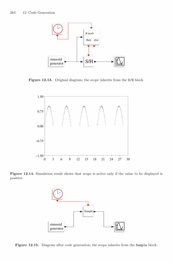
264 12 Code Generation
then else
If in>0
then else
If in>0
generatorsinusoidgeneratorsinusoid S/HS/H
Figure 12.13. Original diagram; the scope inherits from the S/H block.
0 3 6 9 12 15 18 21 24 27 30−1.50
−0.75
0.00
0.75
1.50
+
++++++++++++++++++++++
++++++++++ +
++++++++++++++++++++++
+++++++++++ +
+++++++++++++++
+++++++++++++++++ ++
++++++++++++++
+++++++++++++++++ +
+++++++++++++++++++++
+++++++++++
Figure 12.14. Simulation result shows that scope is active only if the value to be displayed ispositive.
generatorsinusoidgeneratorsinusoid
SampleSample
Figure 12.15. Diagram after code generation; the scope inherits from the Sample block.
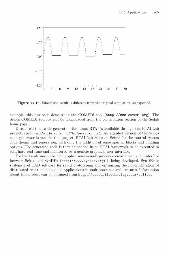
12.5 Applications 265
0 3 6 9 12 15 18 21 24 27 30−1.50
−0.75
0.00
0.75
1.50
+
++++++++++++++++++++++
++++++++++++++++++++++++++++++++++++++++++++
++++++++++++++++++++++
++++++++++++++++++++++++++++++++++++++++++++
+++++++++++++++
+++++++++++++++++++++++++++++++++++++++++++++++++++
+++++++++++++++
++++++++++++++++++++++++++++++++++++++++++++++++++++
+++++++++++++++++++++
++++++++++++++++++++++++++++
Figure 12.16. Simulation result is different from the original simulation, as expected.
example, this has been done using the COMEDI tool (http://www.comedi.org). TheScicos COMEDI toolbox can be downloaded from the contribution section of the Scilabhome page.
Direct real-time code generation for Linux RTAI is available through the RTAI-Labproject; see http://a.die.supsi.ch/~bucher/rtai.html. An adapted version of the Scicoscode generator is used in this project. RTAI-Lab relies on Scicos for the control systemcode design and generation, with only the addition of some specific blocks and buildingoptions. The generated code is then embedded in an RTAI framework to be executed insoft/hard real time and monitored by a generic graphical user interface.
For hard real-time embedded applications in multiprocessor environments, an interfacebetween Scicos and SynDEx (http://www.syndex.org) is being developed. SynDEx issystem-level CAD software for rapid prototyping and optimizing the implementation ofdistributed real-time embedded applications in multiprocessor architectures. Informationabout this project can be obtained from http://www.criltechnology.com/eclipse.

13
Debugging
When a large Scicos diagram does not yield the expected simulation results, it can befairly complicated to identify the problem. To help the user, debugging tools are providedin Scicos. We shall present these tools later in this chapter, but we will first explain Scicoserror messages.
13.1 Error Messages
When something goes wrong during the simulation, the simulation stops and an error mes-sage is displayed. Problems encountered by the simulator can be of a number of differenttypes.
13.1.1 Block Errors
An error could occur within a block, or more specifically the computational function ofthe block. These errors must be signaled by the block itself using the set block errorfunction, which should be called with a negative value depending on the type of errorencountered. The following error flag values can be used:
• −1: This means that a block has been called with input out of its domain. In general,this means that one of the input arguments of the computational function does nothave the expected value. The block can print out, in a Scilab menu, more details usingthe scifunc function.
• −2: This error is signaled if the block encounters a singularity, that is, an operationsuch as division by zero.
• −16: This error corresponds to the case that a block wants to allocate memory (forwhich it has to use the scicos malloc function) but it cannot.
Another block-related error, not detected by the block itself but by the simulator, happenswhen the block tries to program an event on an output activation port but the eventpreviously programmed on the same activation port has not been fired. This happens, forexample, if an event delay block is activated with an event clock and the period of theclock is smaller than the delay period in the delay block.
Finally, it could happen that Scicos simply cannot find the block’s computationalfunction. This could happen with a user block if the computational function is not linked inScilab before simulation or its name does not match the name in the model data structureof the block (set by the interfacing function). The message in this case is unknown block.
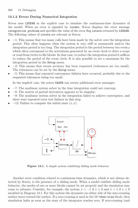
268 13 Debugging
13.1.2 Errors During Numerical Integration
Scicos uses LSODAR in the explicit case to simulate the continuous-time dynamics ofthe model. When an error is signaled by lsodat, Scicos displays the error messageintegration problem and specifies the value of the error flag istate returned by LSODAR.The following values of istate are relevant in Scicos.
• −1: This means that too many calls have been made by the solver over the integrationperiod. This often happens when the system is very stiff or nonsmooth and/or theintegration period is too long. The integration period is the period between two event,swhich often correspond to the activations generated by an event clock to drive a scopeor read-from/write-to file blocks. In that case, to reduce the integration period it sufficesto reduce the period of the event clock. It is also possible to set a maximum for theintegration period in the Setup menu.
• −2: This means that excess accuracy has been requested (tolerances are too small).The tolerances can be set by the Setup menu.
• −5: This means that repeated convergence failures have occurred, probably due to therequested tolerances being too small.
In the implicit case, the solver DASKR can return additional error messages:
• −7: The nonlinear system solver in the time integration could not converge.• −8: The matrix of partial derivatives appears to be singular.• −9: The nonlinear system solver in the integration failed to achieve convergence, and
there were repeated error test failures in this step.• −12: Failure to compute the initial state (x, x).
−1−1
then else
If in>0
then else
If in>0
11SelectorSelector
1/sMScopeMScope
Figure 13.1. A simple system exhibiting sliding mode behavior.
Another error condition related to continuous-time dynamics, which is not always de-tected by Scicos, is the presence of a sliding mode. When a model exhibits sliding modebehavior, the modes of one or more blocks cannot be set properly and the simulation maycease to advance. Consider, for example, the system x = −1 if x ≥ 0 and x = 1 if x < 0modeled in Diagram 13.1. For this system the dynamics on either side of the zero-crossingsurface move toward the surface. If a zero-crossing is used in the If-then-else block, thensimulation halts as soon as the state of the integrator reaches zero. If zero-crossing (and
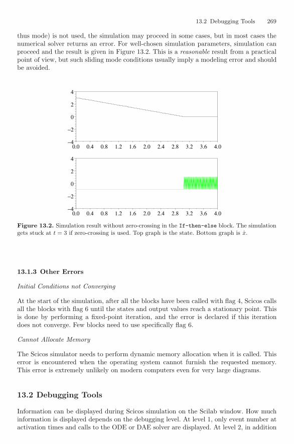
13.2 Debugging Tools 269
thus mode) is not used, the simulation may proceed in some cases, but in most cases thenumerical solver returns an error. For well-chosen simulation parameters, simulation canproceed and the result is given in Figure 13.2. This is a reasonable result from a practicalpoint of view, but such sliding mode conditions usually imply a modeling error and shouldbe avoided.
0.0 0.4 0.8 1.2 1.6 2.0 2.4 2.8 3.2 3.6 4.0−4
−2
0
2
4
+
0.0 0.4 0.8 1.2 1.6 2.0 2.4 2.8 3.2 3.6 4.0−4
−2
0
2
4
+
Figure 13.2. Simulation result without zero-crossing in the If-then-else block. The simulationgets stuck at t = 3 if zero-crossing is used. Top graph is the state. Bottom graph is x.
13.1.3 Other Errors
Initial Conditions not Converging
At the start of the simulation, after all the blocks have been called with flag 4, Scicos callsall the blocks with flag 6 until the states and output values reach a stationary point. Thisis done by performing a fixed-point iteration, and the error is declared if this iterationdoes not converge. Few blocks need to use specifically flag 6.
Cannot Allocate Memory
The Scicos simulator needs to perform dynamic memory allocation when it is called. Thiserror is encountered when the operating system cannot furnish the requested memory.This error is extremely unlikely on modern computers even for very large diagrams.
13.2 Debugging Tools
Information can be displayed during Scicos simulation on the Scilab window. How muchinformation is displayed depends on the debugging level. At level 1, only event number atactivation times and calls to the ODE or DAE solver are displayed. At level 2, in addition
270 13 Debugging
to the information displayed at level 1, the block number and activation time of everyactivated block is displayed.
The debugging level can be set to i by the Scilab command
scicos_debug(i)
It can also be set by a Scicos menu. If i is zero, the debugging is turned off.In most cases, the display of information is not enough to efficiently debug Scicos
diagrams. That is why Scicos provides a powerful debugging facility through the Debugblock (in the Others palette). This block should be placed in the diagram being debugged.
The Debug block has a Scilab computational function of type 99. This type of blockis not activated itself but it impersonates all the other blocks in the diagram, once beforeand once after their activations, provided the debug level is set to 2. The debug level isautomatically set to 2 when the dialog box of the Debug block is opened and validated.
In the dialog box of the Debug block, it is possible to place Scilab instructions to beexecuted when the computational function of the Debug block is called. This means oncebefore and once after each block activation. The default instruction in the dialog box of theDebug block is pause. This corresponds to a simulation in single-step mode. Under pause,all the block parameters can be inspected and even modified. To stop the debugging, itsuffices to set the debugging level back to zero as follows:
-1-> scicos_debug(0)
Having the possibility to use any Scilab instructions provides a powerful debuggingenvironment. For example, the pause statement can be made conditional:
if flag==1&scicos_time()>3&curblock()==2&block.inptr(1)>0 then
pause
end
This way, the user can choose exactly where and when the pause should occur. But manyother Scilab instructions can be used, as we shall see in the examples later. In theseinstructions, we have access to the environment available to any Scilab computationalfunction of type 5. We have seen in the above example the use of functions scicos timeand curblock. The other functions available to type 5 blocks presented on page 206 canalso be used, in addition to the function scicos debug count, which returns the numberof times the block Debug has been called.
In addition to these functions, which provide information about the block, the Scilabfunction getscicosvars can be used to obtain information about the global state of themodel, in particular x, z, and outtb. The continuous-time state x is obtained by thecommand getscicosvars(‘‘x’’), etc.
Other information that can be obtained from getscicosvars is xptr, zptr, rpar,rpptr, ipar, ipptr, inpptr, outptr, inplnk, outlnk, and lnkptr. These variables arepart of %cpr.sim and do not evolve as a function of time. They are essential in deter-mining which parts of x, z, and outtb correspond to which block. For more details, seeAppendix A.
13.3 Examples
The Debug block can be used in various ways to supervise, analyze, and debug a Scicosdiagram. Here we present two elementary examples to illustrate the possibilities. Typicalapplications are, of course, in general a lot more complex.
13.3 Examples 271
13.3.1 Log File
The Debug block can be used to create a log file including information concerning everysingle call to every block. The information recorded in the log file can be more or lessdetailed. Here we record the time, the block number, the values of inputs, and the computedvalues of the outputs. We do not consider the states or the way they are updated. It is forthis reason that we consider only the case of flag equal to 1 in simulation phase 1. Thefollowing statements are placed inside the Debug block:
if flag==1&phase_simulation()==1 then
unit=mopen(’scicoslog.dat’,’a’)
if scicos_debug_count()==1 then mfprintf(unit,’SIMULATION DATE ’+date()+’\n’),end
if scicos_debug_count()-int(scicos_debug_count()/2)*2>0 then
mfprintf(unit,’Block number: %3d at time %5.3f \n’,curblock(),scicos_time())
for i=1:size(block.inptr)
IN=strcat(string(block.inptr(i)’),’;’)
mfprintf(unit,’ Input number ’+string(i)+’ is [’+IN+’]\n’)
end
else
for i=1:size(block.outptr)
OUT=strcat(string(block.outptr(i)’),’;’)
mfprintf(unit,’ Output number ’+string(i)+’ is [’+OUT+’]\n’)
end
end
mclose(unit)
end
Note that the information concerning the inputs is written before the block is called,and the information concerning the outputs is written after the block is called. This isdone by testing whether or not scicos debug count is odd. Since the Debug block iscalled twice for each block execution (once before and once after), if scicos debug countis odd, then it corresponds to a call before block activation.
The information, at each call, is appended to the end of the file scicoslog.dat. Thisfile typically contains
SIMULATION DATE 11-Jan-2005
Block number: 1 at time 0.000
Input number 1 is [-0.0761649]
Output number 1 is [-2;1;2]
Block number: 3 at time 0.000
Input number 1 is [0]
Input number 2 is [-5.1904856;-2.9075105;4.7414013]
Output number 1 is [0;0;0]
Block number: 8 at time 0.000
Output number 1 is [0]
Block number: 2 at time 0.000
Input number 1 is [-2;1;2]
Output number 1 is [3;8]
and so on.
13.3.2 Animation
Here we use the Debug block to animate the block executions on the Scicos editor. This isdone by highlighting a block when it is activated.

272 13 Debugging
xset(’window’,1000) // Main Scicos editor window
k=%cpr.corinv(curblock())
if scicos_debug_count()-int(scicos_debug_count()/2)*2>0 then
hilite_obj(scs_m.objs(k(1)))
else
xpause(50000)
unhilite_obj(scs_m.objs(k(1)))
end
Note that k gives the path to the block to be highlighted, but if the block is inside aSuper block, only the first value of k is used. This means that only the Super block on themain window containing the block is highlighted.
The xpause command is used to make sure that the period of time when the blockremains highlighted is sufficiently long so that it can be seen on screen.
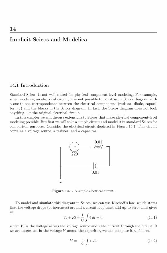
14
Implicit Scicos and Modelica
14.1 Introduction
Standard Scicos is not well suited for physical component-level modeling. For example,when modeling an electrical circuit, it is not possible to construct a Scicos diagram witha one-to-one correspondence between the electrical components (resistor, diode, capaci-tor,. . . ) and the blocks in the Scicos diagram. In fact, the Scicos diagram does not lookanything like the original electrical circuit.
In this chapter we will discuss extensions to Scicos that make physical component-levelmodeling possible. But first we will take a simple circuit and model it in standard Scicos forcomparison purposes. Consider the electrical circuit depicted in Figure 14.1. This circuitcontains a voltage source, a resistor, and a capacitor.
~
220
0.01
0.01
Figure 14.1. A simple electrical circuit.
To model and simulate this diagram in Scicos, we can use Kirchoff’s law, which statesthat the voltage drops (or increases) around a circuit loop must add up to zero. This givesus
Vs + Ri +1C
∫i dt = 0, (14.1)
where Vs is the voltage across the voltage source and i the current through the circuit. Ifwe are interested in the voltage V across the capacitor, we can compute it as follows:
V = − 1C
∫i dt. (14.2)
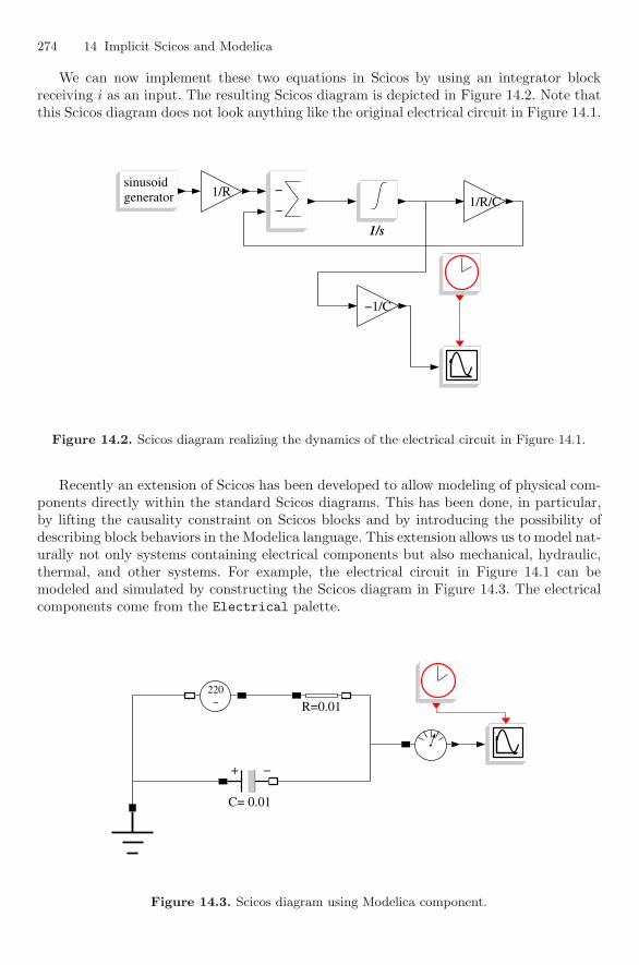
274 14 Implicit Scicos and Modelica
We can now implement these two equations in Scicos by using an integrator blockreceiving i as an input. The resulting Scicos diagram is depicted in Figure 14.2. Note thatthis Scicos diagram does not look anything like the original electrical circuit in Figure 14.1.
1/s
1/R/C1/R/C
−1/C−1/C
1/R1/R −
−
−
−generatorsinusoidgeneratorsinusoid
Figure 14.2. Scicos diagram realizing the dynamics of the electrical circuit in Figure 14.1.
Recently an extension of Scicos has been developed to allow modeling of physical com-ponents directly within the standard Scicos diagrams. This has been done, in particular,by lifting the causality constraint on Scicos blocks and by introducing the possibility ofdescribing block behaviors in the Modelica language. This extension allows us to model nat-urally not only systems containing electrical components but also mechanical, hydraulic,thermal, and other systems. For example, the electrical circuit in Figure 14.1 can bemodeled and simulated by constructing the Scicos diagram in Figure 14.3. The electricalcomponents come from the Electrical palette.
R=0.01R=0.01
+ −
C= 0.01
+ −
C= 0.01
~220~
220
Figure 14.3. Scicos diagram using Modelica component.
14.3 Implicit Blocks 275
The user should be aware that this extension is still being developed and should notbe considered a stable product. In this chapter we provide some information on how touse this facility, but we do not provide detailed documentation because things may changein the future. We also assume that the reader is familiar with Modelica; if not, consultwww.modelica.org for documentation.
14.2 Internally Implicit Blocks
The first step in extending Scicos to accept implicit blocks has been the introduction ofinternally implicit blocks. These blocks are identical to standard Scicos blocks except forthe fact that the internal continuous-time dynamics are allowed to be implicit. This meansthat (9.6) for internally implicit blocks changes to
e(t) = f0(t, x(t), x(t), z(t), u(t), nevprt, μ(t)), (14.3)
where e(t) is the residual, which in theory equals zero, and the solver tries to keep it closeto zero during numerical integration.
Internally implicit blocks have explicit input-output ports and are used in Scicos exactlythe same way as standard blocks are. This means, in particular, that the editor and, exceptfor some minor modifications, the compiler were not affected by the introduction of theseblocks. But the simulator had to be extended because a diagram containing even a singleinternally implicit block results in a system of differential algebraic equations (DAE) thatcannot be solved with an ODE solver. It is for this reason that the DAE solver DASKRhad been interfaced with the Scicos simulator. DAEs were discussed earlier, in Chapter 3where the solver dassl was presented. DASKR is a relatively new member of the family;it is DASPK with root-finding added [14].
Solving DAE systems poses specific problems [11], in particular, that of finding con-sistent initial conditions. In the case of a DAE, and in particular an internally implicitblock, the state is not just x but the pair (x, x), and not all pairs (x, x) are consistent withthe system equations. Finding consistent initial conditions can be a complex problem insome cases. This is particularly difficult in the multimode case, which is often encounteredin the Scicos environment. To help the DAE solver find consistent initial conditions, aninternally implicit block must be able to furnish information about the nature of eachstate variable. It should specify in particular which state variables are algebraic and whichones are differential [15]. This is done by the computational function of the block when itis called with flag 7.
We do not give detailed information here on how to construct internally implicit blocks.It suffices to say that the computational function is of type 10005, that (x, x) must beplaced in the continuous-time state slot in the model, that the computational functionmust return the residual e(t) when it is called with flag 0 and should provide additionalinformation when called with flag 7.
The reason we do not insist on the details is that one rarely needs to construct suchan internally implicit block. These blocks are generated automatically when the diagramcontains implicit blocks, as will be discussed in the next section.
14.3 Implicit Blocks
Implicit blocks, contrary to internally implicit blocks, have implicit ports. An implicit portis different from an input or an output port in that connecting two such ports imposes a

276 14 Implicit Scicos and Modelica
constraint on the values at these ports but does not imply the transfer of information inan a priori known direction, as is the case when we connect an output port to an inputport. For example, the implicit block Capacitor used in the diagram of Figure 14.3 hascurrent and voltage values on its ports but there is no way a priori, without analyzing thefull diagram, to designate the ports as input or output.
Implicit blocks and the construction of diagrams based on these blocks is fully in thespirit of the object-oriented Modelica language [22]. The description of block behavior inScicos is done in Modelica.1
14.3.1 Scicos Editor
Implicit and regular Scicos blocks can be used in the same diagram. The way implicitblocks are handled by the Scicos editor is similar to the way regular blocks are handled.Blocks can be copied from palettes or inserted using the Add New Block functionality.Two elementary palettes are provided by Scicos. Super blocks can be used to structurediagrams with implicit blocks. Note that Super block implicit ports are available in theSources and Sinks palettes for that. A Super block can have both explicit and implicitports.
Links are constructed as in the regular case. It is, of course, not possible to connect animplicit port to an explicit port (it would be meaningless anyway). The connection to theexplicit world can come only from the implicit blocks having one or more explicit portssuch as the voltage sensor in Diagram 14.3.
14.3.2 Scicos Compiler
The compilation with implicit blocks is again transparent to the user; however, the compilerperforms a first stage compilation by grouping all the implicit blocks into a single internallyimplicit block. This is done by generating a Modelica program for the implicit part of thediagram and generating the computational function of the new internally implicit block.The C program is compiled (this requires a C compiler) and linked with Scilab, and thenew internally implicit block replaces the implicit part of the diagram. The last stages aresimilar to the way code generation works, as we have seen in Chapter 12, except that theuser does not see the implicit blocks being replaced.
After this first compilation stage, the compilation proceeds as with standard Scicosdiagrams, and subsequently, so does the simulation.
14.3.3 Block Construction
As in the case of standard blocks, we need to provide two functions for each new block: aninterfacing function, in Scilab, and a computational function, in Modelica. The interfacingfunction is similar to that of a regular block. The only difference is an additional field inthe model structure and two additional fields in the graphics structure of the block.
model.equations is in fact present in all blocks. But in regular blocks, it is set to anempty list and not used. In the VoltageSensor block, for example, model.equations isdefined as follows:
mo=modelica()
mo.model=’VoltageSensor’
1 For the moment only a subset of the language is implemented.

14.4 Example 277
mo.inputs=’p’;
mo.outputs=[’n’;’v’]
model.equations=mo
Implicit blocks can be classified either as inputs or outputs. Here the Modelica variablein the Modelica class VoltageSensor p is defined as input and n and v as outputs. Butin fact, p and n correspond to implicit ports. The output v is explicit. It measures thevoltage across the block, i.e., between p and n.
The implicit/explicit nature of the input-output ports is characterized in two new fieldsin the graphics structure. In the case of VoltageSensor, we have
graphics.in_implicit=[’I’]
graphics.out_implicit=[’I’;’E’]
The interfacing function of this block, as with the rest of the blocks in the Electricalpalette, can be found in the directory scilab/macros/scicos blocks/Electrical. Thisdirectory contains also the Modelica sources of the blocks.
The Modelica program defining the behavior of the VoltageSensor block can be foundin the file VoltageSensor.mo:
class VoltageSensor
Pin p;
Pin n;
Real v;
equation
p.i = 0;
n.i = 0;
v = p.v - n.v;
end VoltageSensor;
For a Modelica class to be usable in the definition of an implicit block in Scicos,the corresponding .mo file must be precompiled using the Modelica compiler modelicac,available in the directory scilab/bin/modelicac. The result is a file with extension .moc.For example, if the class is named foo and is defined in the file foo.mo, the command
modelicac -c foo.mo
produces a file named foo.moc. To use foo in Scicos, the Scilab variable modelica libsmust include the path to the directory where foo.moc can be found. Initially, the pathsto the directories Electrical and Hydraulics are placed in modelica libs. Paths touser-defined *.moc files must be added by the user to modelica libs before launchingScicos.
14.4 Example
Here we consider the construction and the use of a new implicit block in Scicos. This blockis an ideal operational amplifier (infinite gain) to be used with the electrical componentsalready available in the Electrical palette. The Modelica model of this operational am-plifier is very simple and is taken from the Modelica library Electrical.Analog.Ideal,with small modifications to make it compatible with modelicac:
class IdealOpAmp3Pin
Pin in_p "Positive pin of the input port";
Pin in_n "Negative pin of the input port";
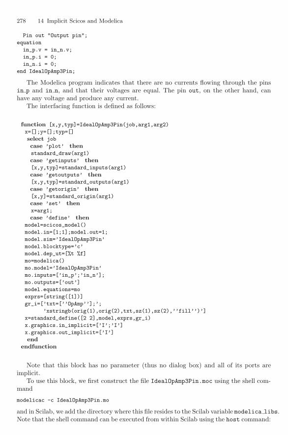
278 14 Implicit Scicos and Modelica
Pin out "Output pin";
equation
in_p.v = in_n.v;
in_p.i = 0;
in_n.i = 0;
end IdealOpAmp3Pin;
The Modelica program indicates that there are no currents flowing through the pinsin p and in n, and that their voltages are equal. The pin out, on the other hand, canhave any voltage and produce any current.
The interfacing function is defined as follows:
function [x,y,typ]=IdealOpAmp3Pin(job,arg1,arg2)
x=[];y=[];typ=[]
select job
case ’plot’ thenstandard_draw(arg1)
case ’getinputs’ then[x,y,typ]=standard_inputs(arg1)
case ’getoutputs’ then[x,y,typ]=standard_outputs(arg1)
case ’getorigin’ then[x,y]=standard_origin(arg1)
case ’set’ thenx=arg1;
case ’define’ thenmodel=scicos_model()
model.in=[1;1];model.out=1;
model.sim=’IdealOpAmp3Pin’
model.blocktype=’c’
model.dep_ut=[%t %f]
mo=modelica()
mo.model=’IdealOpAmp3Pin’
mo.inputs=[’in_p’;’in_n’];
mo.outputs=[’out’]
model.equations=mo
exprs=[string([1])]
gr_i=[’txt=[’’OpAmp’’];’;
’xstringb(orig(1),orig(2),txt,sz(1),sz(2),’’fill’’)’]
x=standard_define([2 2],model,exprs,gr_i)
x.graphics.in_implicit=[’I’;’I’]
x.graphics.out_implicit=[’I’]
endendfunction
Note that this block has no parameter (thus no dialog box) and all of its ports areimplicit.
To use this block, we first construct the file IdealOpAmp3Pin.moc using the shell com-mand
modelicac -c IdealOpAmp3Pin.mo
and in Scilab, we add the directory where this file resides to the Scilab variable modelica libs.Note that the shell command can be executed from within Scilab using the host command:
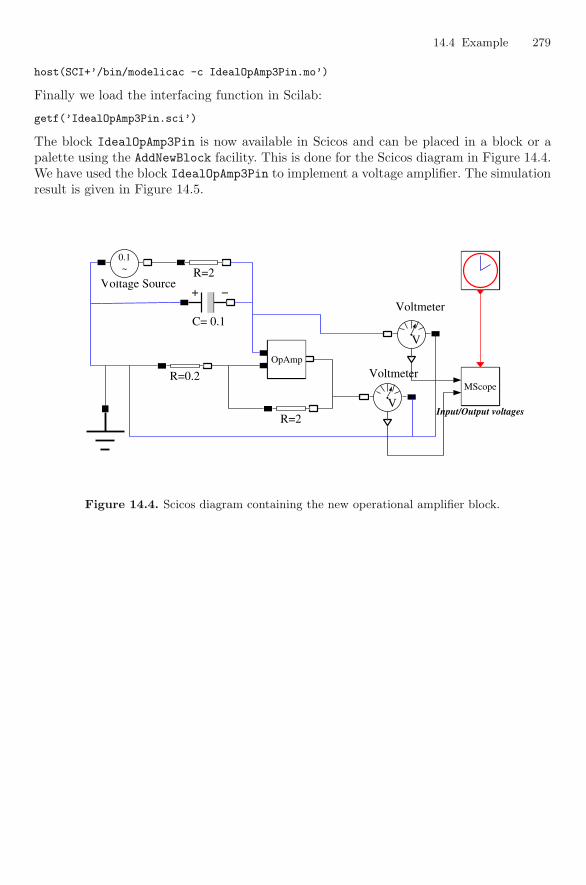
14.4 Example 279
host(SCI+’/bin/modelicac -c IdealOpAmp3Pin.mo’)
Finally we load the interfacing function in Scilab:
getf(’IdealOpAmp3Pin.sci’)
The block IdealOpAmp3Pin is now available in Scicos and can be placed in a block or apalette using the AddNewBlock facility. This is done for the Scicos diagram in Figure 14.4.We have used the block IdealOpAmp3Pin to implement a voltage amplifier. The simulationresult is given in Figure 14.5.
Voltmeter
Voltage Source
VV
~0.1~
0.1
Input/Output voltages
MScopeMScope
R=2R=2
OpAmpOpAmp
R=0.2R=0.2
R=2R=2VV
+ −
C= 0.1
+ −
C= 0.1Voltmeter
Figure 14.4. Scicos diagram containing the new operational amplifier block.

280 14 Implicit Scicos and Modelica
0.0 0.2 0.4 0.6 0.8 1.0 1.2 1.4 1.6 1.8 2.0−0.10
−0.05
0.00
0.05
0.10
+
0.0 0.2 0.4 0.6 0.8 1.0 1.2 1.4 1.6 1.8 2.0−1.0
−0.5
0.0
0.5
1.0
+
Figure 14.5. Simulation result.
A
Inside Scicos
In this chapter, we will give an overview of how the Scicos compiler and editor are im-plemented. This information is useful for advanced users who want to customize Scicos ordevelop exotic functionalities. It is also useful for developers of interfaces to other software.But it can also be of interest to the average user, in particular, for efficiently using thedebugging facilities.
Our objective here is not to give a detailed description of the underlying code but ratherto give enough information so that the code (which of course is available in the sourceversion of Scilab) becomes comprehensible. This requires explaining the data structuresused and giving the structure of the main programs.
The data structures used in Scicos are all Scilab variables. Thus they can be exam-ined and altered using standard Scilab functions. There are in particular two variablesassociated with a Scicos diagram that are of great importance:
• scs m contains all the information concerning the Scicos diagram. It is constructed bythe editor.
• %cpr contains the result of the compilation; it is used by the simulator.
We start with a brief presentation of the editor and the way scs m is constructed. Wethen look at the compilation phase, where scs m is used to obtain %cpr. %cpr is used bythe simulator to perform simulation.
A.1 Scicos Editor
The Scicos editor is written entirely in the Scilab language, including the graphical userinterface, which uses standard Scilab graphics. This facilitates customization of the editorby the user. This section provides the necessary information.
A.1.1 Main Editor Function
The main Scilab function implementing the Scicos editor is scicos, which can be foundin file SCI/macros/auto/scicos.sci. This function takes as input argument a Scicosdiagram (scs m) and opens it. Invoked without any argument, it opens an empty diagram.This function is called recursively when a Super block is opened.
The Scicos editor can be parameterized by initializing the following variables:
282 A Inside Scicos
• scicos pal: list of palettes. An n×2 matrix of strings, where the first column containsthe names of the palettes and the second the file (.cos or .cosf) in which the paletteis defined. In fact, a palette is nothing but a Scicos diagram.
• %scicos menu: Scicos menus. A Scilab list including vectors of strings, where the firstelement of each vector contains the name of the menu, and the rest, the correspondingitems of the menu. Each item corresponds to an operation (such as move, copy, save)and has a corresponding Scilab function.
• %scicos short: keyboard shortcuts. An n×2 matrix of strings, where the first columncontains the character to be used for the shortcut (only lower-case characters can beused) and the second, the name of an operation, which must be an item in one of themenus.
• %scicos help: manual pages associated with operations. A Scilab tlist where foreach operation, a vector of strings contains the corresponding manual page.
• %scicos display mode: this scalar is used to specify whether backstoring for graphicaldisplay of the diagrams should be used by the editor.
• modelica libs: a vector of strings containing the list of directories (full path), whereimplicit Modelica blocks are defined.
• scicos pal libs: a vector of strings containing the list of directories insideSCI/macros/scicos blocks to be loaded. These directories contain the interfacingfunctions of the blocks in Scicos palettes. The user should not, in general, edit thisvariable.
These variables are initialized by the function initial scicos tables, which canbe found in the directory SCI/macros/util. This function is executed as a script byscilab.star, which is executed at the startup of Scilab. They can be modified by theuser subsequently.
The function scicos contains the main event loop of the editor. When an item in oneof the menus is invoked to perform an operation, scicos calls the corresponding Scilabfunction. The name of the Scilab function is derived from the name of the menu item byremoving special characters “/”, “.”, and “-”, and adding a trailing “ ”. For example, thefunction corresponding to the item Open/set in the Object menu is OpenSet . Functionsassociated with editor operations have no input-output arguments and are executed asscripts. Scicos comes with default menus providing many elementary editor operations.The associated functions can be found in the directory SCI/macros/scicos.
Example
Here we give an example of adding a new operation to the Scicos editor. This is just a toyexample and consists in analyzing the diagram and displaying the number of blocks, thenumber of Super blocks, and the number of links in the diagram. We start by adding anew item, which we call Block Info. We place it in the last position. For that, the Scilabvariable %scicos menu should be modified. This should be done before Scicos is launched.
Default Scicos menus are Diagram, Edit, Simulate, Object, and Misc. So if we wantto place this item in Misc, we should add it to the vector %scicos menu(5). For example,it can be placed at the end of this menu.
By doing so, the item Diagram Info is added to the Misc menu in Scicos, and whenthe user selects this item, Scicos attempts to execute the function DiagramInfo . So weneed to define this function as well. To implement fully the debugging menu, the followingscript can be used.
These instructions must be executed before Scicos is launched. A convenient place forthem is in the .scilab file.

A.1 Scicos Editor 283
%scicos_menu($)($+1)="Diagram Info";
function [block_num,link_num,sup_num]=..
do_diagram_Info(scs_m,block_num,link_num,sup_num)
for i=1:length(scs_m.objs)
if typeof(scs_m.objs(i))==’Block’ thenif or(scs_m.objs(i).model.sim==[’super’,’csuper’]) thensup_num=sup_num+1;
[block_num,link_num,sup_num]=..
do_diagram_Info(scs_m.objs(i).model.rpar,block_num,link_num,sup_num)
elseif ~or(scs_m.objs(i).model.sim==[’input’,’output’]) thenblock_num=block_num+1;
endelseif typeof(scs_m.objs(i))==’Link’ thenlink_num=link_num+1;
endend
endfunction
function DiagramInfo_()
[block_num,link_num,sup_num]=do_diagram_Info(scs_m,0,0,0);
txt=["Number of basic blocks: "+string(block_num);
"Number of Super blocks: "+string(sup_num);
"Number of links: "+string(link_num)];
message(txt)
Cmenu="Open/Set"
endfunction
Note that in order to explore the scs m structure, we examine each item in the objsfield and increment the corresponding counters. When a Super block is encountered, thefunction do diagram Info is called recursively. This way we can explore the content ofthe hierarchical structure scs m.
The Cmenu variable sets the next operation to be performed. By default in Scicos, theeditor is in Open/Set operation mode.
Editor operations are, in general, more complex and involve Scilab variables definedand used in scicos. For example, in most cases, an operation modifies the variable scs m,which codes the current status of the diagram. The best way to learn about these variablesis by examining source codes of the functions associated with default operations.
A.1.2 Structure of scs m
scs m is a Scilab object of type diagram having two entries:
• props: Diagram properties. Scilab object of type params,• objs: list of objects included in the Scicos diagram.
Diagram Properties params
The diagram properties are:
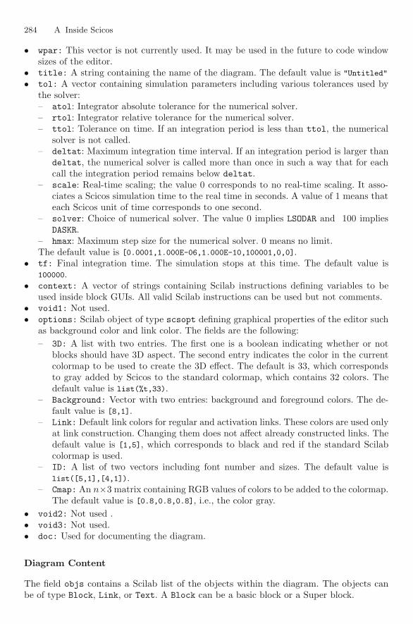
284 A Inside Scicos
• wpar: This vector is not currently used. It may be used in the future to code windowsizes of the editor.
• title: A string containing the name of the diagram. The default value is "Untitled"
• tol: A vector containing simulation parameters including various tolerances used bythe solver:– atol: Integrator absolute tolerance for the numerical solver.– rtol: Integrator relative tolerance for the numerical solver.– ttol: Tolerance on time. If an integration period is less than ttol, the numerical
solver is not called.– deltat: Maximum integration time interval. If an integration period is larger than
deltat, the numerical solver is called more than once in such a way that for eachcall the integration period remains below deltat.
– scale: Real-time scaling; the value 0 corresponds to no real-time scaling. It asso-ciates a Scicos simulation time to the real time in seconds. A value of 1 means thateach Scicos unit of time corresponds to one second.
– solver: Choice of numerical solver. The value 0 implies LSODAR and 100 impliesDASKR.
– hmax: Maximum step size for the numerical solver. 0 means no limit.The default value is [0.0001,1.000E-06,1.000E-10,100001,0,0].
• tf: Final integration time. The simulation stops at this time. The default value is100000.
• context: A vector of strings containing Scilab instructions defining variables to beused inside block GUIs. All valid Scilab instructions can be used but not comments.
• void1: Not used.• options: Scilab object of type scsopt defining graphical properties of the editor such
as background color and link color. The fields are the following:– 3D: A list with two entries. The first one is a boolean indicating whether or not
blocks should have 3D aspect. The second entry indicates the color in the currentcolormap to be used to create the 3D effect. The default is 33, which correspondsto gray added by Scicos to the standard colormap, which contains 32 colors. Thedefault value is list(%t,33).
– Background: Vector with two entries: background and foreground colors. The de-fault value is [8,1].
– Link: Default link colors for regular and activation links. These colors are used onlyat link construction. Changing them does not affect already constructed links. Thedefault value is [1,5], which corresponds to black and red if the standard Scilabcolormap is used.
– ID: A list of two vectors including font number and sizes. The default value islist([5,1],[4,1]).
– Cmap: An n×3 matrix containing RGB values of colors to be added to the colormap.The default value is [0.8,0.8,0.8], i.e., the color gray.
• void2: Not used .• void3: Not used.• doc: Used for documenting the diagram.
Diagram Content
The field objs contains a Scilab list of the objects within the diagram. The objects canbe of type Block, Link, or Text. A Block can be a basic block or a Super block.
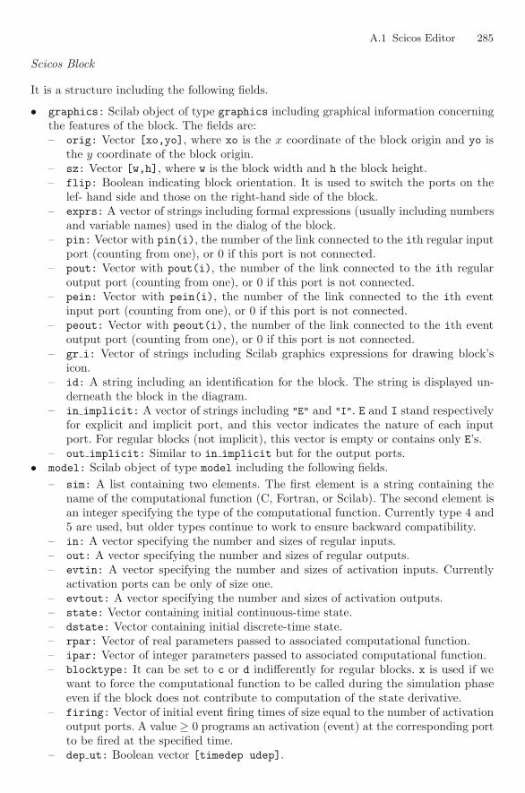
A.1 Scicos Editor 285
Scicos Block
It is a structure including the following fields.
• graphics: Scilab object of type graphics including graphical information concerningthe features of the block. The fields are:– orig: Vector [xo,yo], where xo is the x coordinate of the block origin and yo is
the y coordinate of the block origin.– sz: Vector [w,h], where w is the block width and h the block height.– flip: Boolean indicating block orientation. It is used to switch the ports on the
lef- hand side and those on the right-hand side of the block.– exprs: A vector of strings including formal expressions (usually including numbers
and variable names) used in the dialog of the block.– pin: Vector with pin(i), the number of the link connected to the ith regular input
port (counting from one), or 0 if this port is not connected.– pout: Vector with pout(i), the number of the link connected to the ith regular
output port (counting from one), or 0 if this port is not connected.– pein: Vector with pein(i), the number of the link connected to the ith event
input port (counting from one), or 0 if this port is not connected.– peout: Vector with peout(i), the number of the link connected to the ith event
output port (counting from one), or 0 if this port is not connected.– gr i: Vector of strings including Scilab graphics expressions for drawing block’s
icon.– id: A string including an identification for the block. The string is displayed un-
derneath the block in the diagram.– in implicit: A vector of strings including "E" and "I". E and I stand respectively
for explicit and implicit port, and this vector indicates the nature of each inputport. For regular blocks (not implicit), this vector is empty or contains only E’s.
– out implicit: Similar to in implicit but for the output ports.• model: Scilab object of type model including the following fields.
– sim: A list containing two elements. The first element is a string containing thename of the computational function (C, Fortran, or Scilab). The second element isan integer specifying the type of the computational function. Currently type 4 and5 are used, but older types continue to work to ensure backward compatibility.
– in: A vector specifying the number and sizes of regular inputs.– out: A vector specifying the number and sizes of regular outputs.– evtin: A vector specifying the number and sizes of activation inputs. Currently
activation ports can be only of size one.– evtout: A vector specifying the number and sizes of activation outputs.– state: Vector containing initial continuous-time state.– dstate: Vector containing initial discrete-time state.– rpar: Vector of real parameters passed to associated computational function.– ipar: Vector of integer parameters passed to associated computational function.– blocktype: It can be set to c or d indifferently for regular blocks. x is used if we
want to force the computational function to be called during the simulation phaseeven if the block does not contribute to computation of the state derivative.
– firing: Vector of initial event firing times of size equal to the number of activationoutput ports. A value ≥ 0 programs an activation (event) at the corresponding portto be fired at the specified time.
– dep ut: Boolean vector [timedep udep].
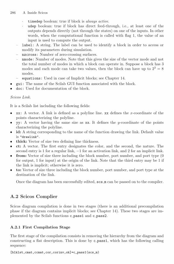
286 A Inside Scicos
· timedep boolean: true if block is always active.· udep boolean: true if block has direct feed-through, i.e., at least one of the
outputs depends directly (not through the states) on one of the inputs. In otherwords, when the computational function is called with flag 1, the value of aninput is used to compute the output.
– label: A string. The label can be used to identify a block in order to access ormodify its parameters during simulation.
– nzcross: Number of zero-crossing surfaces.– nmode: Number of modes. Note that this gives the size of the vector mode and not
the total number of modes in which a block can operate in. Suppose a block has 3modes and each mode can take two values, then the block can have up to 23 = 8modes.
– equations: Used in case of Implicit blocks; see Chapter 14.• gui: The name of the Scilab GUI function associated with the block.• doc: Used for documentation of the block.
Scicos Link.
It is a Scilab list including the following fields:
• xx: A vector. A link is defined as a polyline line. xx defines the x-coordinate of thepoints characterizing the polyline.
• yy: A vector having the same size as xx. It defines the y-coordinate of the pointscharacterizing the polyline.
• id: A string corresponding to the name of the function drawing the link. Default valueis "drawlink".
• thick: Vector of size two defining line thickness.• ct: A vector. The first entry designates the color, and the second, the nature. The
second entry is 1 for a regular link, −1 for an activation link, and 2 for an implicit link.• from: Vector of size three including the block number, port number, and port type (0
for output, 1 for input) at the origin of the link. Note that the third entry may be 1 ifthe link is implicit; otherwise it is zero.
• to: Vector of size three including the block number, port number, and port type at thedestination of the link.
Once the diagram has been successfully edited, scs m can be passed on to the compiler.
A.2 Scicos Complier
Scicos diagram compilation is done in two stages (there is an additional precompilationphase if the diagram contains implicit blocks; see Chapter 14). These two stages are im-plemented by the Scilab functions c pass1 and c pass2.
A.2.1 First Compilation Stage
The first stage of the compilation consists in removing the hierarchy from the diagram andconstructing a flat description. This is done by c pass1, which has the following callingsequence:
[blklst,cmat,ccmat,cor,corinv,ok]=c_pass1(scs_m)
A.2 Scicos Complier 287
• blklst is a list of blocks present in the diagram. It contains block information relevantto simulation. Block properties such as color, icon, size, and location, which are notuseful for simulation, have been stripped.
• cmat is an n×6 matrix. Each row corresponds to a regular link and contains the blocknumber, port number, and port type (explicit or implicit) of the source block and thesame information regarding the destination block.
• ccmat is an n× 4 matrix. Each row corresponds to an activation link and contains theblock number and port number of the source block and the block number and portnumber of the destination block.
• cor and corinv are correspondence tables (coded as lists) used to find the correspon-dence between blocks in blklst and scs m.
A.2.2 Second Compilation Stage
The second stage is done by the main compilation function c pass2, which constructs allthe scheduling tables and other information needed for simulation and code generation.The calling sequence is as follows:
%cpr=c_pass2(blklst,connectmat,ccmat,cor,corinv)
The input arguments are all generated by c pass1. connectmat is simply cmat, butthe third and last columns have been removed. The output %cpr is a Scilab structurecontaining all the information needed by the simulator. We will not explain how c pass2computes %cpr. Instead we give a detailed description of %cpr in the next section.
A.2.3 Structure of %cpr
The Scilab object %cpr contains the result of the compilation. The simulator uses only%cpr. It is thus important for an advanced user to understand how compilation results arecoded in %cpr.
• state: Scilab object of type xcs. It contains all the states of the model, that is,everything than can evolve during the simulation. It contains in particular– x: The continuous-time state, which is obtained by concatenating the continuous-
time states of all the blocks.– z: The discrete-time state, which is obtained by concatenating the discrete-time
states of all the blocks.– iz: Vector of size equal to the number of blocks. If a block needs to allocate memory
at initialization, the associated pointer is saved here.– tevts: Vector of size equal to the number of activation sources. It contains the
scheduled times for programmed activations.– evtspt: Vector of size equal to the number of activation sources. It is an event
scheduler.– pointi: The number of the next programmed event.– outtb: Vector containing all the link memories. Link memories hold block output
values.• sim: Scilab object of type scs. It contains information that does not evolve during the
simulation.– funs: A vector containing the name of the computational functions.– xptr: A vector pointer to the continuous time state x. The continuous-time state
of block i is%cpr.state.x(%cpr.sim.xptr(i):%cpr.sim.xptr(i+1)-1).
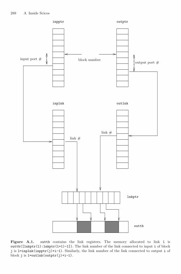
288 A Inside Scicos
outptr
inplnk outlnk
lnkptr
outtb
input port #output port #
block number
inpptr
link #
link #
Figure A.1. outtb contains the link registers. The memory allocated to link l isouttb([lnkptr(l):lnkptr(l+1)-1]). The link number of the link connected to input i of blockj is l=inplnk(inpptr(j)+i-1). Similarly, the link number of the link connected to output i ofblock j is l=outlnk(outptr(j)+i-1).
A.2 Scicos Complier 289
– zptr: A vector pointer to the discrete-time state z, which is similar to xptr.– zcptr: A vector pointer to the zero-crossing surfaces.– inpptr: A vector pointer used to find the link number and consequently the part
of outtb corresponding to a given input port. See Figure A.1.– outptr: Similar to inpptr but for output ports.– inplnk: Similar to inpptr. See Figure A.1.– outlnk: Similar to inplnk but for output ports.– lnkptr: A vector pointer to outtb indicating the region corresponding to a given
link.– rpar: Vector of real parameters that is obtained by concatenating the real param-
eters of all the blocks.– rpptr: A vector pointer to real parameters rpar. The real parameters of block i
are%cpr.sim.rpar(%cpr.sim.rpptr(i):%cpr.sim.rpptr(i+1)-1).
– ipar: Vector of integer parameters, similar to rpar.– ipptr: A vector pointer to integer parameters, similar to rpptr.– clkptr: A vector pointer to output activation ports.– ordptr: A vector pointer to ordclk designating the part of ordclk corresponding
to a given activation.– execlk: Not used.– ordclk: An n×2 matrix associated to blocks activated by output activation ports.
The first column contains the block number, and the second, the event code bywhich the block should be called. See Figure A.2.
– cord: An n×2 matrix associated to always active blocks. The first column containsthe block number, and the second, the event code by which the block should becalled.
– oord: Subset of cord, which affects the continuous-time state derivative.– zord: Subset of cord, which affects the computation of zero-crossing surfaces.– critev: A vector of size equal to the number of activations and containing zeros
and ones. The value one indicates that the activation is critical in the sense thatthe continuous-time solver must be cold restarted.
– nb: Number of blocks. Note that the number of blocks may differ from the originalnumber of blocks in the diagram because c pass2 may duplicate some conditionalblocks.
– ztyp: A vector of size equal to the number of blocks. A 1 entry indicates thatthe block may have zero-crossings, even if it doesn’t in the context of the diagram.Usually not used by the simulator.
– nblk: Not used. Set to nb.– ndcblk: Not used.– subscr: Not used.– funtyp: A vector of size equal to the number of blocks indicating the type of the
computational function of the block. Block type can be 0 through 5. Currently onlytype 4 (C language) and type 5 (Scilab language) computational functions shouldbe used. But older blocks can also be used.
– iord: An n × 2 matrix associated to blocks that must be activated at the startof the simulation. This includes blocks inheriting from constant blocks and alwaysactive blocks.
– labels: A string vector of size equal to the number of blocks containing blocklabels.
– modptr: A vector pointer to the block modes.
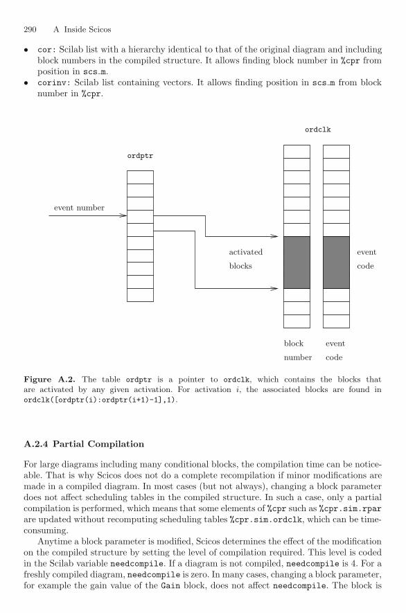
290 A Inside Scicos
• cor: Scilab list with a hierarchy identical to that of the original diagram and includingblock numbers in the compiled structure. It allows finding block number in %cpr fromposition in scs m.
• corinv: Scilab list containing vectors. It allows finding position in scs m from blocknumber in %cpr.
ordptr
ordclk
event number
activated
blocks
event
code
block
number code
event
Figure A.2. The table ordptr is a pointer to ordclk, which contains the blocks thatare activated by any given activation. For activation i, the associated blocks are found inordclk([ordptr(i):ordptr(i+1)-1],1).
A.2.4 Partial Compilation
For large diagrams including many conditional blocks, the compilation time can be notice-able. That is why Scicos does not do a complete recompilation if minor modifications aremade in a compiled diagram. In most cases (but not always), changing a block parameterdoes not affect scheduling tables in the compiled structure. In such a case, only a partialcompilation is performed, which means that some elements of %cpr such as %cpr.sim.rparare updated without recomputing scheduling tables %cpr.sim.ordclk, which can be time-consuming.
Anytime a block parameter is modified, Scicos determines the effect of the modificationon the compiled structure by setting the level of compilation required. This level is codedin the Scilab variable needcompile. If a diagram is not compiled, needcompile is 4. For afreshly compiled diagram, needcompile is zero. In many cases, changing a block parameter,for example the gain value of the Gain block, does not affect needcompile. The block is
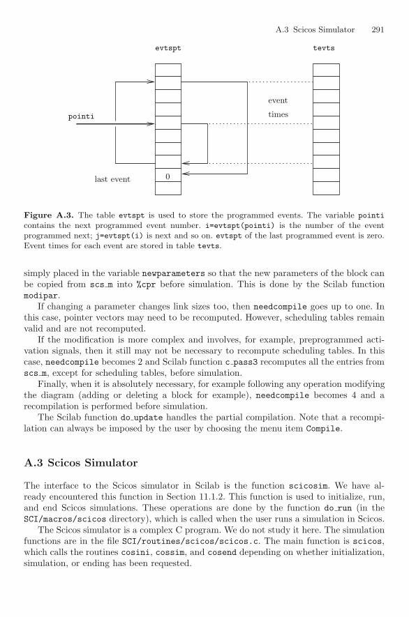
A.3 Scicos Simulator 291
evtspt tevts
0last event
pointi
event
times
Figure A.3. The table evtspt is used to store the programmed events. The variable pointi
contains the next programmed event number. i=evtspt(pointi) is the number of the eventprogrammed next; j=evtspt(i) is next and so on. evtspt of the last programmed event is zero.Event times for each event are stored in table tevts.
simply placed in the variable newparameters so that the new parameters of the block canbe copied from scs m into %cpr before simulation. This is done by the Scilab functionmodipar.
If changing a parameter changes link sizes too, then needcompile goes up to one. Inthis case, pointer vectors may need to be recomputed. However, scheduling tables remainvalid and are not recomputed.
If the modification is more complex and involves, for example, preprogrammed acti-vation signals, then it still may not be necessary to recompute scheduling tables. In thiscase, needcompile becomes 2 and Scilab function c pass3 recomputes all the entries fromscs m, except for scheduling tables, before simulation.
Finally, when it is absolutely necessary, for example following any operation modifyingthe diagram (adding or deleting a block for example), needcompile becomes 4 and arecompilation is performed before simulation.
The Scilab function do update handles the partial compilation. Note that a recompi-lation can always be imposed by the user by choosing the menu item Compile.
A.3 Scicos Simulator
The interface to the Scicos simulator in Scilab is the function scicosim. We have al-ready encountered this function in Section 11.1.2. This function is used to initialize, run,and end Scicos simulations. These operations are done by the function do run (in theSCI/macros/scicos directory), which is called when the user runs a simulation in Scicos.
The Scicos simulator is a complex C program. We do not study it here. The simulationfunctions are in the file SCI/routines/scicos/scicos.c. The main function is scicos,which calls the routines cosini, cossim, and cosend depending on whether initialization,simulation, or ending has been requested.
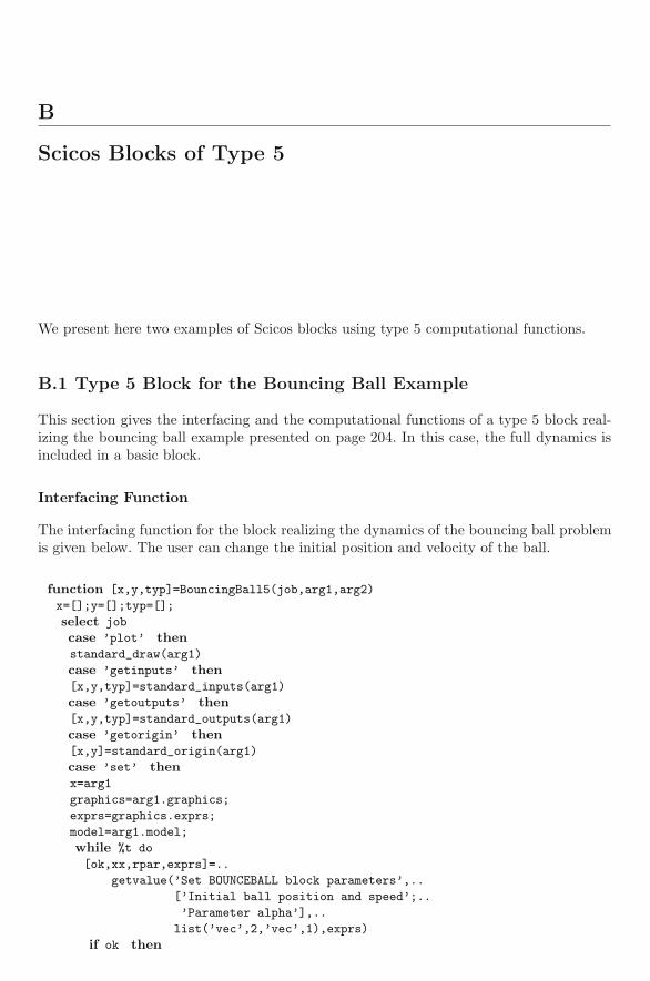
B
Scicos Blocks of Type 5
We present here two examples of Scicos blocks using type 5 computational functions.
B.1 Type 5 Block for the Bouncing Ball Example
This section gives the interfacing and the computational functions of a type 5 block real-izing the bouncing ball example presented on page 204. In this case, the full dynamics isincluded in a basic block.
Interfacing Function
The interfacing function for the block realizing the dynamics of the bouncing ball problemis given below. The user can change the initial position and velocity of the ball.
function [x,y,typ]=BouncingBall5(job,arg1,arg2)
x=[];y=[];typ=[];
select job
case ’plot’ thenstandard_draw(arg1)
case ’getinputs’ then[x,y,typ]=standard_inputs(arg1)
case ’getoutputs’ then[x,y,typ]=standard_outputs(arg1)
case ’getorigin’ then[x,y]=standard_origin(arg1)
case ’set’ thenx=arg1
graphics=arg1.graphics;
exprs=graphics.exprs;
model=arg1.model;
while %t do
[ok,xx,rpar,exprs]=..
getvalue(’Set BOUNCEBALL block parameters’,..
[’Initial ball position and speed’;..
’Parameter alpha’],..
list(’vec’,2,’vec’,1),exprs)
if ok then
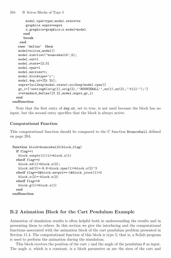
294 B Scicos Blocks of Type 5
model.rpar=rpar;model.state=xx
graphics.exprs=exprs
x.graphics=graphics;x.model=model
endbreak
endcase ’define’ thenmodel=scicos_model()
model.sim=list(’bounceball5’,5);
model.out=1
model.state=[2;0]
model.rpar=1
model.nzcross=1;
model.blocktype=’c’;
model.dep_ut=[%t %t];
exprs=[sci2exp(model.state);sci2exp(model.rpar)]
gr_i=[’xstringb(orig(1),orig(2),’’BOUNCEBALL’’,sz(1),sz(2),’’fill’’);’]
x=standard_define([3 2],model,exprs,gr_i)
endendfunction
Note that the first entry of dep ut, set to true, is not used because the block has noinput, but the second entry specifies that the block is always active.
Computational Function
This computational function should be compared to the C function Bounceball definedon page 204.
function block=bounceball5(block,flag)
if flag==1
block.outptr(1)(1)=block.x(1)
elseif flag==0
block.xd(1)=block.x(2);
block.xd(2)=-9.8-block.rpar(1)*block.x(2)^3
elseif flag==2&block.nevprt==-1&block.jroot(1)<0
block.x(2)=-block.x(2)
elseif flag==9
block.g(1)=block.x(1)
endendfunction
B.2 Animation Block for the Cart Pendulum Example
Animation of simulation results is often helpful both in understanding the results and inpresenting them to others. In this section we give the interfacing and the computationalfunctions associated with the animation block of the cart pendulum problem presented inSection 11.4. The computational function of this block is type 5; that is, a Scilab programis used to perform the animation during the simulation.
This block receives the position of the cart z and the angle of the pendulum θ as input.The angle φ, which is a constant, is a block parameter as are the sizes of the cart and
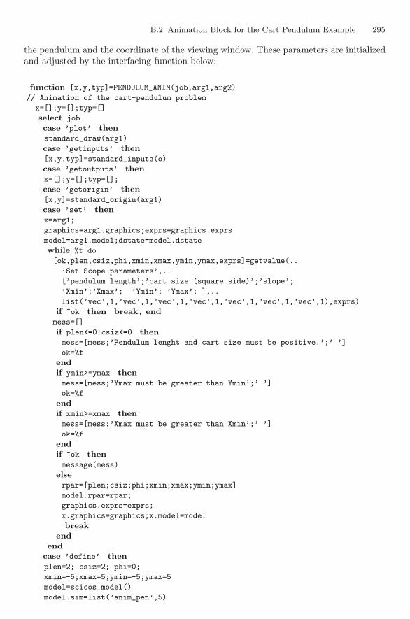
B.2 Animation Block for the Cart Pendulum Example 295
the pendulum and the coordinate of the viewing window. These parameters are initializedand adjusted by the interfacing function below:
function [x,y,typ]=PENDULUM_ANIM(job,arg1,arg2)
// Animation of the cart-pendulum problem
x=[];y=[];typ=[]
select job
case ’plot’ thenstandard_draw(arg1)
case ’getinputs’ then[x,y,typ]=standard_inputs(o)
case ’getoutputs’ thenx=[];y=[];typ=[];
case ’getorigin’ then[x,y]=standard_origin(arg1)
case ’set’ thenx=arg1;
graphics=arg1.graphics;exprs=graphics.exprs
model=arg1.model;dstate=model.dstate
while %t do
[ok,plen,csiz,phi,xmin,xmax,ymin,ymax,exprs]=getvalue(..
’Set Scope parameters’,..
[’pendulum length’;’cart size (square side)’;’slope’;
’Xmin’;’Xmax’; ’Ymin’; ’Ymax’; ],..
list(’vec’,1,’vec’,1,’vec’,1,’vec’,1,’vec’,1,’vec’,1,’vec’,1),exprs)
if ~ok then break, endmess=[]
if plen<=0|csiz<=0 thenmess=[mess;’Pendulum lenght and cart size must be positive.’;’ ’]
ok=%f
endif ymin>=ymax thenmess=[mess;’Ymax must be greater than Ymin’;’ ’]
ok=%f
endif xmin>=xmax thenmess=[mess;’Xmax must be greater than Xmin’;’ ’]
ok=%f
endif ~ok thenmessage(mess)
elserpar=[plen;csiz;phi;xmin;xmax;ymin;ymax]
model.rpar=rpar;
graphics.exprs=exprs;
x.graphics=graphics;x.model=model
breakend
endcase ’define’ thenplen=2; csiz=2; phi=0;
xmin=-5;xmax=5;ymin=-5;ymax=5
model=scicos_model()
model.sim=list(’anim_pen’,5)
296 B Scicos Blocks of Type 5
model.in=[1;1]
model.evtin=1
model.dstate=0
model.rpar=[plen;csiz;phi;xmin;xmax;ymin;ymax]
model.blocktype=’d’
model.dep_ut=[%f %f]
exprs=string(model.rpar)
gr_i=[’thick=xget(’’thickness’’);xset(’’thickness’’,2);’;
’xx=orig(1)+sz(1)*[.40.60.60.40.4]’
’yy=orig(2)+sz(2)*[.20.20.40.40.2]’
’xpoly(xx,yy,’’lines’’)’
’xx=orig(1)+sz(1)*[.50.6]’
’yy=orig(2)+sz(2)*[.40.8]’
’xpoly(xx,yy)’
’xset(’’thickness’’,thick);’]
x=standard_define([3 3],model,exprs,gr_i)
endendfunction
Note that this block has 2 regular scalar inputs and an activation input. The activationinput receives during the simulation the information concerning the time instants whenthe display has to be updated. Note also that the block has a discrete-time state, set tozero. The reason for the presence of this state is to make sure that during the simulation,the block is called with flag equal to 2. Since this block has no output (from the pointof view of Scicos; there is indeed an output to the screen), the block is never called withflag equal to 1. So in the absence of a state, the block is never called during simulation.Adding a state is one way to overcome this problem. The other is to add outputs to theblock. This latter method works even if these outputs are left unconnected. Here we havechosen to add a state, which turns out to be useful for other reasons.
The computational function of this block is defined in PENDULUM ANIM to be anim pen.This function is given below.
function [blocks] = anim_pen(blocks,flag)
win=20000+curblock()
if flag<>4 then H=scf(win), endxold=blocks.z
rpar=blocks.rpar
plen=rpar(1);csiz=rpar(2);phi=rpar(3);
if flag==4 thenxset("window",win)
set("figure_style","new")
H=scf(win)
clf(H)
H.pixmap=’on’
Axe=H.children
Axe.data_bounds=rpar(4:7)
Axe.isoview=’on’
S=[cos(phi),-sin(phi);sin(phi),cos(phi)]
XY=S*[rpar(4),rpar(5);-csiz/2,-csiz/2]
xsegs(XY(1,:),XY(2,:))
x=0;theta=0;
x1=x-csiz/2;x2=x+csiz/2;y1=-csiz/2;y2=csiz/2

B.2 Animation Block for the Cart Pendulum Example 297
XY=S*[x1 x2 x2 x1 x1;y1,y1,y2,y2,y1]
xpoly(XY(1,:),XY(2,:),"lines",1)
XY=S*[x,x+plen*sin(theta);0,0+plen*cos(theta)]
xsegs(XY(1,:),XY(2,:))
elseif flag==2 thenAxe=H.children
x=blocks.inptr(1)(1)
theta=blocks.inptr(2)(1)
XY=Axe.children(2).data’+..
[cos(phi)*(x-xold);sin(phi)*(x-xold)]*ones(1,5)
Axe.children(2).data=XY’
x1=x*cos(phi);y1=x*sin(phi)
XY=[x1,x1+plen*sin(theta);y1,y1+plen*cos(theta)]
Axe.children(1).data=XY’
blocks.z=x
show_pixmap()
endendfunction
This block uses Scilab’s new graphics (in contrast to Scicos, which still uses the oldgraphics). The window number of the graphical display is set to 20000 plus the blocknumber. This is to make sure that if two such blocks are used in the same diagram, theyuse different windows for their displays. The discrete-time state blocks.z, which has beenintroduced simply to make sure the block is called during simulation, is also used to storethe previous position of the cart. This information is then used to update the associatedgraphics data structure in a slightly more efficient way. This is done by computing thechange in the position by subtracting the old position from the new position.
The isoview property is used to make sure the horizontal and vertical scales remainproportional on the screen after resizing the window. The pixmap mode is used to createan efficient and smooth animation. In particular, the display is refreshed only after all thechanges have been done. Note that the block does not ensure real-time simulation. Thismust be done by adjusting the corresponding simulation parameter of the diagram.
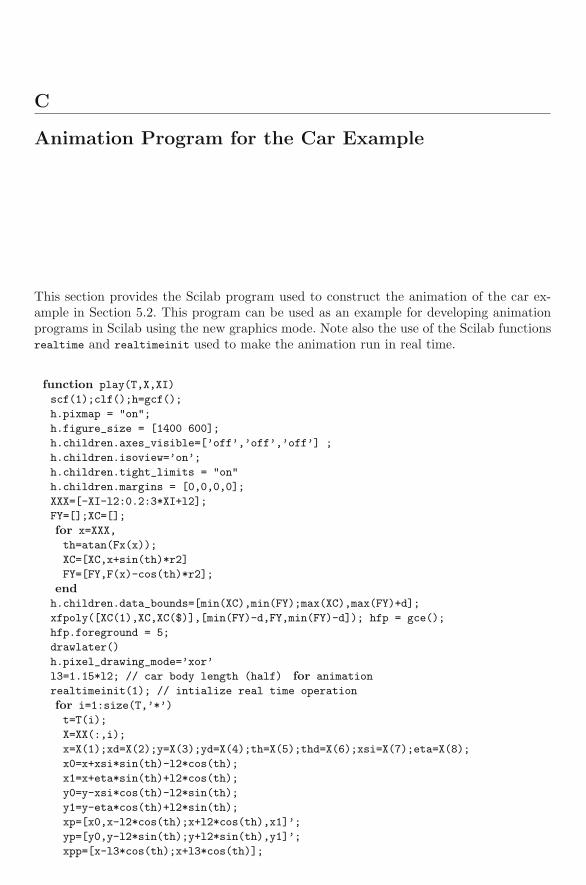
C
Animation Program for the Car Example
This section provides the Scilab program used to construct the animation of the car ex-ample in Section 5.2. This program can be used as an example for developing animationprograms in Scilab using the new graphics mode. Note also the use of the Scilab functionsrealtime and realtimeinit used to make the animation run in real time.
function play(T,X,XI)
scf(1);clf();h=gcf();
h.pixmap = "on";
h.figure_size = [1400 600];
h.children.axes_visible=[’off’,’off’,’off’] ;
h.children.isoview=’on’;
h.children.tight_limits = "on"
h.children.margins = [0,0,0,0];
XXX=[-XI-l2:0.2:3*XI+l2];
FY=[];XC=[];
for x=XXX,
th=atan(Fx(x));
XC=[XC,x+sin(th)*r2]
FY=[FY,F(x)-cos(th)*r2];
endh.children.data_bounds=[min(XC),min(FY);max(XC),max(FY)+d];
xfpoly([XC(1),XC,XC($)],[min(FY)-d,FY,min(FY)-d]); hfp = gce();
hfp.foreground = 5;
drawlater()
h.pixel_drawing_mode=’xor’
l3=1.15*l2; // car body length (half) for animation
realtimeinit(1); // intialize real time operation
for i=1:size(T,’*’)
t=T(i);
X=XX(:,i);
x=X(1);xd=X(2);y=X(3);yd=X(4);th=X(5);thd=X(6);xsi=X(7);eta=X(8);
x0=x+xsi*sin(th)-l2*cos(th);
x1=x+eta*sin(th)+l2*cos(th);
y0=y-xsi*cos(th)-l2*sin(th);
y1=y-eta*cos(th)+l2*sin(th);
xp=[x0,x-l2*cos(th);x+l2*cos(th),x1]’;
yp=[y0,y-l2*sin(th);y+l2*sin(th),y1]’;
xpp=[x-l3*cos(th);x+l3*cos(th)];
300 C Animation Program for the Car Example
ypp=[y-l3*sin(th);y+l3*sin(th)];
W1=[x0-r2,y0+r2,2*r2,2*r2,0,360*64];
W2=[x1-r2,y1+r2,2*r2,2*r2,0,360*64];
if i==1 thenxpoly(xpp,ypp); hp1 = gce();
hp1.thickness=10;
xpolys(xp,yp); hp2 = gce();hp21=hp2.children(1);hp22=hp2.children(2)
xfarcs([W1’,W2’]); ha = gce();ha1=ha.children(1);ha2=ha.children(2)
realtime(t);
draw([hp1,hp2,ha])//draw car
elsedraw([hp1,hp2,ha])//erase car
hp1.data=[xpp,ypp];
hp21.data=[xp(:,1),yp(:,1)];
hp22.data=[xp(:,2),yp(:,2)];
ha1.data=W1;
ha2.data=W2;
realtime(t);
draw([hp1,hp2,ha])//draw car
endshow_pixmap()
endh.pixel_drawing_mode=’copy’
drawnow()
show_pixmap()
endfunction

D
Extraction Program for the LATEX Graphic Example
This function exports to a file in mixed LATEX and Postscript code the content of a Scilabgraphic window. This file has been in particular used in Section 2.4.4 to produce the twofiles figps-ps.eps and figps-tex.tex.
function xs2latex(win,fname)
base=basename(fname);
I=strindex(base,’.’);
if I==[] thenfname_eps= fname+’.eps’;
fname= fname+’.ps’;
elsesuf=part(fname,I($):length(fname));
if suf<>".ps" thenerror(’xs2latex: fname must be ended by0.ps’);
return;
endfname_eps= part(fname,1:I($-1))+’.eps’;
end;xs2ps(win,fname)
unix(SCI+’/bin/Blatexpr 1 1 ’+fname);
txt=mgetl(fname_eps);
I=grep(txt,"%Latex:");
txt1=txt(I);
I=grep(txt1,"nan");
txt1(I)=[];
txt1=strsubst(txt1,"%Latex:","");
mputl(txt1,base+’-tex.tex’);
txt1=txt;
I=[];
for i=1:size(txt,’*’)
i,
l=length(txt(i));
if l-4 >= 1 thenif part(txt(i),(l-4):l) == " Show" then I=[I,i]; end
endendtxt1(I)=[];
mputl(txt1,base+’-ps.eps’);

302 D Extraction Program for the LATEX Graphic Example
endfunction
E
Maple Code Used for Modeling the N -Link Pendulum
Here we give the Maple code for the N -link pendulum presented in Section 5.1. We haveremoved from the Maple code functions devoted to LATEX code generation and to energycomputation (ener.f).
read(‘Euler.map‘);
#---------------------------------------------------------------------------------
# Lagrangian for the N-link pendulum ( l[i]: length of links r[i]:=l[i]/2;)
#---------------------------------------------------------------------------------
# number of links in the pendulum
n:=2;
# [x,y,theta] is of size three
mm:=3:
LLi:=proc(i)
(1/2)*m[i]*( ( xd[i-1]- r[i] *sin(th[i])*thd[i])**2 +
( yd[i-1]+ r[i]*cos(th[i])*thd[i])**2 ) + 1/2*J[i]*(thd[i])**2
-m[i]*g*(y[i-1]+r[i]*sin(th[i])):
end:
# The point zero is fixed
x[0]:=0:xd[0]:=0: y[0]:=0:yd[0]:=0:
L:=sum( LLi(j),j=1..n):
# Lagrangian variables:
q := [ seq (op([x[i],y[i],th[i]]),i=1..n)]:
qd := [ seq (op([xd[i],yd[i],thd[i]]),i=1..n)]:
qdd:= [ seq (op([xdd[i],ydd[i],thdd[i]]),i=1..n)]:
# Lhs of Euler equations
EL:=euler_equations(L,q,qd,qdd): EE:=map((i)->rhs(i),EL):
#-----------------------------------------------------
# Rewriting the Euler equations to have a canonical form
# used only for output
304 E Maple Code Used for Modeling the N -Link Pendulum
#-----------------------------------------------------
XX:=CEuler(EE,q,qd,qdd):
ME1:=XX[1]:
ME1:=subs(seq(m[k]*r[k]*cos(th[k])=mrc[k],k=1..n),
seq(m[k]*r[k]*sin(th[k])=mrs[k],k=1..n),eval(ME1)):
#------------------------------------------------
# Constraints on the N-link Pendulum
#------------------------------------------------
ncont:=2*n;
cont:=[ seq(op([ x[i]-x[i-1] - 2*r[i]*cos(th[i]),
y[i]-y[i-1] - 2*r[i]*sin(th[i])]),i=1..n)]:
# time derivative of constraints;
cont1:=map ( (exp)->( time_diff(exp,q,qd,qdd)),cont):
# derivatives of constraints are of type Aprim qd = 0
Aprim:=genmatrix(cont1,qd):
#----------------------------------------------
# Computing S(q);
#----------------------------------------------
SS:=linsolve(Aprim,matrix(ncont,1,0)):
#--------------------------------------------------------------
# Since the indices can be mixed we have to change SS
# so that the correspondence between the eta[i] and the thd[i]
# will be the identity. This is convenient, but not essential,
# in order to have a simple interpretation of eta
#--------------------------------------------------------------
permut:=seq(SS[mm*i,1]=t_s[i],i=1..n): SS:=subs(permut,eval(SS)):
permut:=seq(t_s[i]=eta[i],i=1..n): SS:=subs(permut,eval(SS)):
S:= genmatrix(convert(convert(SS,vector),list),[seq( eta[i],i=1..n)]):
#-----------------------------------------------------
# Left multiplication in the Euler equations.
#-----------------------------------------------------
E1:=multiply(transpose(S),EE):
#-----------------------------------------------------
# .
# q= S(q) eta ; here eta = [eta1,eta2,...]
# ..
# we use this equation to compute q
#-----------------------------------------------------
qt := [ seq (eta[i] ,i=1..n)]: qtd := [ seq (etad[i] ,i=1..n)]:
qtdd:= [ seq (etadd[i],i=1..n)]:
qqdd:=map((x,y,z,t)-> time_diff(x,y,z,t),eval(SS),
E Maple Code Used for Modeling the N -Link Pendulum 305
[op(q),op(qt)],[op(qd),op(qtd)],[op(qdd),op(qtdd)]):
#-----------------------------------------------------
# .. .
# Using q= d/dt [ S(q) eta] and q= S(q) eta
# we can substitute these expressions in E1
#-----------------------------------------------------
E2:=subs(seq(qdd[i]=qqdd[i,1],i=1..nops(qdd)),eval(E1)):
E3:=subs(seq(qd[i]=SS[i,1],i=1..nops(qd)),eval(E2)):
#-----------------------------------------------------
# The global system is now
# .
# E3 = 0 and q= S(q) eta
#-----------------------------------------------------
E3:=map((x)-> simplify(x),E3):
#------------------------------------------------------------------
# Canonical representation for the simplified Euler equations
# .
# El= ME(q) eta + RE(q,eta).
# We use CEuler with a little trick in the parameter call qt,qt,qtd
#------------------------------------------------------------------
XX1:=CEuler(E3,qt,qt,qtd):
MM3:=map((i)->factor(combine(i,trig)),XX1[1]):
RR3:=map((i)->factor(combine(i,trig)),XX1[2]):
#-----------------------------------------------------
# FORTRAN GENERATION
# First routine npend(neq,t,th,ydot)
#-----------------------------------------------------
flist:=[subroutinem,‘npend‘,[‘neq‘,‘t‘,‘th‘,‘ydot‘],
[
[ parameterf,[‘n=‘.n]],
[ declaref,‘implicit doubleprecision‘,[‘(t)‘] ],
[ declaref,doubleprecision,[‘t,th(2*n),eta(n),ydot(2*n),r(n)‘]],
[ declaref,doubleprecision,[‘me3s(n,n),const(n,1),j(n),m(n)‘]],
[ declaref,doubleprecision,[‘w(3*n),rcond ‘]],
[ declaref,integer,[‘i,k,neq,ierr‘]],
[ declaref,‘data g‘,[‘/ 9.81/‘]],
[ declaref,‘data r‘,[‘/ n*1.0/‘] ],
[ declaref,‘data m‘,[‘/ n*1.0/‘] ],
[ declaref,‘data j‘,[‘/ n*0.3/‘] ],
[ dom , ‘i ‘ ,1,‘n ‘,1,[ equalf,‘ydot(i)‘,‘th(i+n)‘]],
[ dom , ‘i ‘ ,1,‘n ‘,1,[ equalf,‘eta(i)‘,‘th(i+n)‘]],
[ matrixm,‘me3s‘,MM3 ] ,
[ matrixm,‘const‘, RR3 ] ,
[ dom , ‘i ‘ ,1,‘n ‘,1,[ equalf,‘const(i,1)‘,‘-const(i,1)‘]],
[commentf,‘ solving M z = const to obtain ydot((n+1)..2*n)‘],
[ callf , ‘dlslv‘,[‘me3s,n,n,const,n,1,w, rcond,ierr,1‘]],
306 E Maple Code Used for Modeling the N -Link Pendulum
[ if_then_m,ierr<>0,[
[writef,6,ff_w,[]],
[formatf,ff_w,[‘’Matrix is badly conditioned’‘]]]],
[ dom , ‘i ‘ ,1,‘n ‘,1,[ equalf,‘ydot(n+i)‘,‘const(i,1)‘]],
[returnf]]]:
Gener(‘npend.f‘,flist):
# New np.f
flist:=[subroutinem,‘np‘,[‘i ‘],
[[ declaref,integer,[‘i ‘]],[ equalf,‘i ‘,n],[returnf]]]:
Gener(‘np.f‘,flist):
References
1. Y. Alain. Theorie et analyse du signal. Cours et initiation pratique via Matlab et Scilab.Ellipses, Paris, 1999.
2. G. Allaire and S. Kaber. Algebre lineaire numerique. Cours et exercices. Ellipses, Paris, 2002.3. G. Allaire and S. Kaber. Introduction a Scilab - Exercices pratiques corriges d’algebre lineaire.
Ellipses, Paris, 2002.4. E. Anderson, Z. Bai, C. Bischof, S. Blackford, J. Demmel, J. Dongarra, J. D. Croz, A. Green-
baum, S. Hammarling, A. McKenney, and D. Sorensen. LAPACK Users’ Guide, Third Edi-tion. SIAM, Philadelphia, 1999.
5. R. M. Anderson and R. M. May. Infectious diseases of humans: dynamics and control. OxfordUniversity Press, Oxford, UK, 1991.
6. U. Ascher, J. Christiansen, and R. D. Russell. A collocation solver for mixed order systemsof boundary value problems. Math. Computation, 33:659–679, 1979.
7. U. Ascher, J. Christiansen, and R. D. Russell. Algorithm 569: Colsys: Collocation software forboundary-value ODEs. ACM Transactions on Mathematical Software (TOMS), 7(2):223–229,1981.
8. U. Ascher, J. Christiansen, and R. D. Russell. Collocation software for boundary-value ODEs.ACM Transactions on Mathematical Software (TOMS), 7(2):209–222, 1981.
9. J. Baumgarte. Stabilization of constraints and integrals of motion in dynamical systems.Comp. Math. Appl. Mech. Eng., 1972.
10. J. T. Betts. Practical Methods for Optimal Control Using Nonlinear Programming. SIAM,2001.
11. K. E. Brenan, S. L. Campbell, and L. R. Petzold. The Numerical Solution of Initial ValueProblems in Differential-Algebraic Equations. SIAM, 1996.
12. D. Brown, A. Herbison, J. Robinson, R. Marrs, and G. Leng. Modelling the luteinizinghormone-releasing hormone pulse generator. Neuroscience, 63(3):869–879, 1994.
13. P. N. Brown and A. C. Hindmarsh. Reduced storage matrix methods in stiff ODE systems.J. Appl. Math. Computation, 31:40–91, 1989.
14. P. N. Brown, A. C. Hindmarsh, and L. R. Petzold. Using Krylov methods in the solution oflarge-scale differential-algebraic systems. SIAM J. Sci. Comp., 15:1467–1488, 1994.
15. P. N. Brown, A. C. Hindmarsh, and L. R. Petzold. Consistent initial condition calculationfor differential-algebraic systems. SIAM Journal on Scientific Computing, 1998.
16. C. Bunks, J. Chancelier, F. Delebecque, C. Gomez, M. Goursat, R. Nikoukhah, and S. Steer.Engineering and Scientific Computing with Scilab. Birkhauser, 1999.
17. M. Caracotsios and W. E. Stewart. Sensitivity analysis of initial value problems with mixedODEs and algebraic equations. Comp. Chem. Eng., 9(4):359–365, 1985.
18. J. Chancelier, F. Delebecque, C. Gomez, M. Goursat, R. Nikoukhah, and S. Steer. Introductiona Scilab. Springer, 2001.
19. W. R. Cowell, editor. Sources and Development of Mathematical Software. Prentice-HallSeries in Computational Mathematics, Cleve Moler, Advisor. Prentice-Hall, Upper SaddleRiver, NJ 07458, USA, 1984.

308 References
20. C. Deboor and R. Weiss. Solveblok: a package for solving almost block diagonal linear systems.ACM Transactions Mathematical Software, 6:80–87, 1980.
21. F. Delebecque and R. Nikoukhah. A mixed symbolic-numeric software environment and itsapplication to control system engineering, pages 221–244. Elsevier Science Publishers, 1992.
22. P. Fritzson. Principles of Object-Oriented Modeling and Simulation with Modelica 2.1. Wiley-IEEE Press, 2004.
23. M. Goossens, F. Mittelbach, and A. Samarin. The LATEXCompanion. Addison Wesley, Read-ing, Massachusets, 1994.
24. A. Griewank, D. Juedes, H. Mitev, J. Utke, O. Vogel, and A. Walther. ADOL-C: A packagefor the automatic differentiation of algorithms written in C/C++: Algor. 755. ACM TOMS,22(2):131–167, 1996.
25. S. Guerre-Delabriere and M. Postel. Methodes d’approximation - Equations differentielles -Applications Scilab. Niveau L3. Ellipses, Paris, 2004.
26. E. Hairer, S. P. Norsett, and G. Wanner. Solving Ordinary Differential Equations I. NonstiffProblems, volume 8 of Springer Series in Comput. Mathematics. Springer-Verlag, 1993.
27. E. Hairer and G. Wanner. Solving Ordinary Differential Equations II. Stiff and Differential-Algebraic Problems, volume 14 of Springer Series in Comput. Mathematics. Springer-Verlag,1991.
28. A. C. Hindmarsh. ODEPACK, A Systematized Collection of ODE Solvers, in Scientific Com-puting. vol. 1 of IMACS Transactions on Scientific Computation. North-Holland, Amsterdam,1983.
29. C. V. Hollot and Y. Chait. Nonlinear stability analysis for a class of tcp/aqm networks.In Proc. of the 40th IEEE Conference on Decision and Control, pages 2309–2314, Orlando,Florida, December 2001.
30. F. L. Lewis. Optimal Control. Wiley, 1986.31. T. Maly and L. Petzold. Numerical methods and software for sensitivity analysis of
differential-algebraic systems. Applied Numerical Mathematics, 20:57–79, 1996.32. W. Michiels and S.-I. Niculescu. Stability analysis of a fluid flow model for tcp like behavior.
International Journal of Bifurcation and Chaos, page to appear, July 2005.33. P. S. M. Pires and D. A. Rogers. Free/open source software: An alternative for engineering
students. In Proc. 32nd ASEE/IEEE Frontiers in Education Conference, pages T3G–7 TO11, Boston, MA, 2002.
34. K. Radhakrishnan and A. C. Hindmarsh. Description and use of LSODE, the livermore solverfor ordinary differential equations. Technical Report report UCRL-ID-113855, Lawrence Liv-ermore National Laboratory, December 1993.
35. O. E. Rossler. An equation for continuous chaos. Phys. Lett., 35A:397–398, 1976.
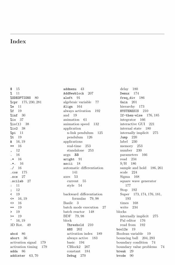
Index
$ 15% 11%ODEOPTIONS 80%cpr 175, 230, 281%e 11%f 19%inf 30%io 37%io(1) 38%io2 38%pi 11%t 19& 16, 19** 16, 12. 16.* 16.*. 16./ 16.cos 175.sce 27.scilab 27: 11; 12< 19<= 16, 19<> 16== 19> 19>= 19~ 16, 193D Rot. 49
abcd 86abort 36activation signal 179activation timing 179adda 86addinter 63, 70
addmenu 43AddNewblock 207aleft 91algebraic variable 77Align 164always activation 192and 19animation 61animation speed 132application
n-link pendulum 125pendulum 126
applicationsreal-time 253standalone 253
argn 33aright 91ascii 18automatic differentiation
141axes 53
current 55style 54
backward differentiationformulas 79, 98
Basile 3batch mode execution 27batch reactor 148BDF 79, 98blockThreshold 210ABS 202activation index 189always active 183basic 194CBlock2 207constant 184Debug 270
delay 180Demux 174freq_div 186Gain 201hierarchy 173HYSTERESIS 210If-then-else 176, 185integrator 166interactive GUI 221internal state 180internally implicit 275Jump 220label 230memory 253number 230parameters 166read 234S/H 186sample and hold 186, 261scale 224Sigma 168square wave generator
177Stop 192Super 173, 174, 176, 181,
193times 168write 234
blocksinternally implicit 275Pal editor 176read from 192
bool2s 19Boolean variable 19bouncing ball 204, 293boundary condition 74boundary value problems 74break 29bvode 90

310 Index
BVP 74
C2F 66call 63cd 42chdir 42CheckLhs 68CheckRhs 68clear 9, 27clf 48clock 164code generation 253
file names 256procedure 256
code2str 232COLNEW 90colormap 56, 58COLSYS 90COMEDI 265command history 5comparison operators 19computational function 195,
197, 294, 296type 5 205
concatenationcolumn 12row 12
conditional subsampling 186conjugate gradient 111constraint
bound 107box 107holonomic 126nonholonomic 126
constraint drift 127context 171control design 249Control flowelse 28elseif 28if 28then 28
control panel 225create_palette 208CreateVar 68csim 87impuls 87
csslti 195curblock 206, 225
DAE 76, 128, 147, 275index zero 85
dasrt 100DASSL 98dassl 128
datafit 117, 147, 241Debug
log file 271decimation operation 184deff 78delay differential equations
221delmenu 43Demos 5dep_t 183dep_u 181derivative 120, 122dgetrf 66diag 13difference equation 75differential algebraic equation
76, 147, 275differential equation
implicit 128differential variable 77differentiation
numerical 120stabilized 127
dir 42discrete 95disease spread 167disp 28, 37dom 86down-sampling 213download 7drawlater 55drawnow 55driver 60dscr 171dsimul 97
Edit 164eigenvalue assignment 171elseif 28emacs 5entity 54%eps 10equations
implicit 275nonlinear 108
equilibrium 248errcatch 19error 33eval 173eval3dp 51event 77event clock 165event generator 164event mechanism 216
Example_events 256exec 27, 36execstr 18existence and uniqueness 74exists 9exp 14expm 14extensions 27eye 13
factorial 31failure detection 213false 19fast Fourier transform 213fchamp 50feedback 212FFT 213Figure 54figure 46figure_style 54file 37File operations 7fileinfo 42find 20, 30fink 3, 4first-order 73, 76fit_dat 117fixpnt 92flts 97fopen 38for 29formatformat 38big endian 41little endian 41native 41
fplot3d 49fsolve 112, 149FSQP 109full 21fully implicit 77, 86functionsfunction 31definition 26, 31
gca() 55gcf() 55gda() 55gdf() 55GENERIC 195get 53getcwd 42getf 27getfield 22GetRhsVar 68

Index 311
getscicosvars 270global 34gradient 108, 110
approximation 109computation 147numerical 120
grand 13graph
editing 49graphic
editing 54export 49functions 56handle 54mode setting 54primitives 56
graphics modenew 53, 132old 60
grep 18%gtk 42guess 93
Hamiltonian 93helpapropos 6browser window 6help 6
Hessian 122histplot 51, 58HOME 27hormone pulse generator
218host 42, 232hybrid 77, 135hybrid system 100hypermat 12, 22
ilib_build 69ilib_for_link 63, 131, 204impl 85implicit differential equation
85implicit semiexplicit DAE
77index of a DAE 76initial condition 74
consistent 76, 148input ports 179INRIA 3int 13int16 11int32 11int8 11interface 66
builder.sce 69examples 68gateway 70interface library 67
interfacing function194, 195, 260, 293,295
inverted pendulum 245, 294ipar 91isdef 9isglobal 34isoview 297
jac 86, 99Jacobian 80
numerical 120job 195jroot 198
Kirchoff’s law 273.*. 13Kronecker product 13
Lagrangian 126LaTeX
psfrag 57least squared 16least squares 113leastsq 113
length 17length 18Levenberg-Marquardt 114LhsVar 68lincos 248line editor 5line style 54linear DAE 85linear program 119linear system 86, 171linearization
scicos 243link
color 165creation 166splitting 166
link 63links
activation 165regular 165
linpro 119linspace 13, 49list 11, 22listfiles 42load 40Load as Palette 176
loader.sce 204logical or 16logspace 13ls 42lsodar 79lsode 79lsqrsolve 113, 155ltitr 97ltol 92
MacOSX 4macros 26malloc 10Maple 126, 130matrix 12matrix 13concatenation 12exponential 14how stored 12multiplication 16sparse 21term by term 16Vandermonde 17
mclose 39mexfiles 69mget 41MINPACK 112mllst 22mode
pixmap 297mode 190mode parameter 191model
fisheries 209predator prey 209
Modelica 274modeling
component-level 273error 269
Monte Carlo 227mopen 38mput 41MSDOS 42msprintf 18msscanf 18multiple shooting 90
ncomp 91NDcost 109nevprt 189node 54norm 17not 19numdiff 120
312 Index
obscont 249observer 171, 212ode 73adams 79atol 79
default value 80discrete 79external 80fix 79fixed step 257jac 80lsoda 79real-time 257rk 79rkf 79root 79rtol 79
default value 80stiff 79type 79
ode 78, 131, 135ode optionsh0 80hmax 80hmin 80itask 80ixpr 81jactype 81maxordn 81maxords 81mi 81mu 81mxstep 81tcrit 80
ode_discrete 95ode_root 87odedc 100ODEPACK 78, 79old_style 54ones 13optim 108, 147optimal control 93or 19ordinary differential equation
73
paletteelectrical 192thermo-hydraulics 192
palettes 159, 192Branching 176, 192copying blocks 163Linear 166Others 174
Sinks 164, 192Sources 164, 192Threshold 192
param3d1 50parameters
symbolic 19318
pathconvert 42pause 35PD controller 225pendulum 125, 245, 294phase_simulation 206PI controller 237pixmap 61play 141plot
editing 49parametric 49surface 49
plot2d 48plot2d2 48plot2d3 48plot2d4 48plot3d 49pmodulo 29points 91Poisson process 216polarplot 51pole placement 171polyline
menu 54poly 20pop 36postscript 49ppol 171, 212, 249primitives 26print 37prompt 4push 36%pvm 42
quadratic program 120quapro 120quasi-Newton 111queuing system 216quit 27, 36
rand 13read 38realtime 132, 299realtimeinit 132, 299Rec 60Region-to-Super-block
173res 85, 98
residual 85resume 35, 36RK4 79RKF45 79root finding 77RTAI 265RTAI-Lab 265rtitr 97
sampled data 101sampled data system 102sampled system 86save 40scale
graphic 61SCI 4Scicos.cosf 175command names 228context 169diagram names 176editor 163error messages 267graphics style 232help 163keyboard shortcuts 163load 175loading 227Misc 163Rename 176Run 165save 175Save-as-Interf-Func
194Setup 165Simulate 165
scicos 163, 281scicos_simulate 232scicos_time 206scicos_ver 175scicosim 228Scierror 68Scifunc 193, 194scilab.ini 27scilab.star 27ScilabEval 44scope 164scripts 27scs 175scs_m 281second derivative
approximation 122select 28
case 28
Index 313
else 28semidef 120semiexplicit DAE 77set 53set_blockerror 206setbpt 36seteventhandler 44setfield 22setmenu 43setpoint 244shooting methods 90sign 18signal processing 184simulation phase 190, 198simulation start time
default 229SIR model 167SISO 87size 206sliding mode 268sparse 21sprand 21stabilization
Baumgarte 127stacksize 10state-space form 86states
continuous-time 190discrete-time 190hybrid 138
steadycos 247, 248step 87stiff 79stop button 166str2code 232strcat 18stream
input 38output 38
strindex 18strings 17string 18concatenation 17
stripblanks 18strsubst 18submatrix
deletion 14extraction 14
subplot 48swap 41Switch 176synchronism 176synchronization 176SynDEx 265syslin 86syslin list 86
Taylor approximation 122Taylor coefficients 122Tck/Tk menus 56Tcl/Tk 44, 223TCL_EvalFile 44TCL_EvalStr 44TCL_ExistVar 44TCL_GetVar 44TCL_SetVar 44%tk 42TCP/AQM Network 221tic 83timer 21, 29tlist 86tlist 11toc 83tokens 18tol 92’ 13true 19type
string 17typeof 9
uicontrol 46uimenu 46Undefined 24unixunix_g 42unix_s 42unix_w 42unix_x 42
unix 42unsetmenu 43
varargin 34vector field 50visible 55Visual C++ 161
web 7where 35whereami 35
while 29, 30who 10whos 10widget 223
definition 222Windows 27windows
dialog 43write 38
x_choices 43x_choose 43x_dialog 43x_mdialog 43x_message 43xbasc 48, 60xbasr 60xclick 44xdel 61xget 61xgetmouse 44xinit 60xload 41xor 142xpause 272xpoly 61xpolys 53xrects 61xrects 52xs2latex 59xs2ps 60xsave 41xset 61clipgrf 52pixmap 61wshow 61thickness 53window 48wwpc 61xtape 60
zero crossing 138, 191zeros 13zeta 91zoom 49