Modeling and Simulation of the Interaction Between ... · Mitarbeiter: Dr. Thomas John___ Eidesstattliche Versicherung Hiermit versichere ich an Eides statt, dass ich die vorliegende

Modeling and Simulation of the Interaction

Between Particles and Pulmonary Mucus

Dissertation zur Erlangung des Grades des Doktors der Naturwissenschaften

der Naturwissenschaftlich-Technischen Fakultät

der Universität des Saarlandes

Matthias Ernst

Saarbrücken

-2017-

Dissertation eingereicht am: _02.02.2017_

1. Gutachter: Prof. Dr. Claus-Michael Lehr

2. Gutachter: __Prof. Dr. Stefan Diebels__

Tag des Kolloquiums: _01.06.2017________

Dekan: _Univ.-Prof. Dr. Guido Kickelbick__

Berichterstatter: Prof. Dr. Claus-Michael Lehr

_ Prof. Dr. Stefan Diebels__

_______________________

Vorsitz: ___Prof. Dr. Christian Wagner_____

Akad. Mitarbeiter: __Dr. Thomas John_____

Eidesstattliche Versicherung

Hiermit versichere ich an Eides statt, dass ich die vorliegende Arbeit selbstständig und ohne

Benutzung anderer als der angegebenen Hilfsmittel angefertigt habe. Die aus anderen Quellen oder

indirekt übernommenen Daten und Konzepte sind unter Angabe der Quelle gekennzeichnet. Die

Arbeit wurde bisher weder im In- noch im Ausland in gleicher oder ähnlicher Form in einem

Verfahren zur Erlangung eines akademischen Grades vorgelegt.

Ort, Datum

(Unterschrift)

1

1 Abstract

The aim of this thesis was to simulate the interaction of particles with the protective barrier of

the lung, the mucus layer. Beginning with different diffusion models to simulate the particle

movement inside the mucus network, we also measured and compared the rheological

properties of mucus from different organs of the same species. Using the results from these

experiments, we simulated the deformation of the mucus structure. We used computational

fluid dynamic (CFD) methods to simulate the air flow in the upper airways during inhalation

and to calculate the kinetic energy of aerosol particles, which are transported by the

convective air flow to depose at the mucus layer. Finally, we did some experiments with

fluorescence recovery after photobleaching (FRAP) methods to visualize the diffusion of

particles in mucus and also the structure of this biological barrier. By applying our model, we

were able to determine the diffusivity of particles in complex, heterogeneous materials, only

by assuming few parameters. So, in this thesis we showed various models to simulate the

interaction, mainly the diffusion, of particles with pulmonary mucus, beginning with the

inhalation and deposition of the particles in the lung and at the mucus layer.

Das Ziel dieser Thesis war die Simulation der Interaktion von Partikeln mit der schützenden

Barriere der Lunge, der Mukusschicht. Angefangen mit verschiedenen Diffusionsmodellen

um die Partikelbewegung innerhalb des Mukus-Netzwerks zu simulieren, haben wir auch die

rheologischen Eigenschaften von Mukus aus verschiedenen Organen der gleichen Spezies

gemessen und verglichen. Wir simulierten die Deformation der Mukus-Struktur mithilfe der

Ergebnisse dieser Experimente. Wir benutzten CFD Methoden um den Luftstrom in den

oberen Atemwegen während der Inhalation zu simulieren und um die kinetische Energie von

Aerosol-Partikel zu berechnen, die durch den konvektiven Luftstrom transportiert werden um

sich auf der Mukusschicht abzusetzen. Letztendlich führten wir noch Experimente mit FRAP

Methoden durch, um die Diffusion von Partikel in Mukus und auch die Struktur dieser

biologischen Barriere darzustellen. Durch die Anwendung unseres Modells sind wir in der

Lage die Diffusivität von Partikeln in komplexen, heterogenen Materialien, alleine mit der

Annahme weniger Parameter zu bestimmen. In dieser Thesis zeigten wir unterschiedliche

Modelle um die Interaktion, hauptsächlich die Diffusion, von Partikeln mit pulmonalem

Mukus zu simulieren, angefangen bei der Inhalation und Ablagerung von Partikeln in der

Lunge und auf der Mukusschicht.

2

1 Abstract 1

2 Table of Contents 2

3 Introduction 5

3.1 Background and significance of the research 5

3.2 State of research and rising problems 6

3.3 Aim of the studies 7

3.4 Workflow and structure of the thesis 8

4 Modeling and Simulation of Particle Diffusion in Mucus 9

4.1 Modeling particle diffusion in mucus and transient subharmonic

behavior based on permeable membranes 9

4.1.1 Introduction 9

4.1.2 Model & numerical methods 15

4.1.3 Results & Discussion 31

4.2 A model to predict particle diffusion in mucus for short and long

time limits 40


4.2.2 Model & experimental findings 41


4.3 Modeling and Simulation of Fickian diffusion based on

concentration gradients and comparison with a Brownian

diffusion model 49


4.3.2 Fickian and Brownian diffusion models 49


4.4 Conclusions 62

3

5 Mechanical and Rheological Properties of Mucus 64

5.1 Introduction 64

5.1.1 Macro- and microrheology of mucus 64

5.1.2 Viscoelastic properties of mucus 64

5.2 Macro- and microrheological properties of native porcine

respiratory and intestinal mucus 66

5.2.1 Material & Methods 66


5.3 Calculation of the necessary deformation energy to expand the

mucus pores 73

5.3.1 Computation of the deflection and deformation of mucin fibers 73

5.3.2 Brownian diffusive energy and comparison with the necessary

deformation energy 80

5.4 Conclusions 81

6 Computational Fluid Dynamics (CFD) Simulations of the

Air Flow in the Human Lung 82

6.1 Introduction 82

6.1.1 Structure of the human lung 82

6.1.2 Development of lung models 83

6.1.3 Particle deposition processes 86

6.1.4 Computational Fluid Dynamics (CFD) 87

6.2 Computation of the velocity profile and the kinetic energy 89

6.2.1 Velocity profile 89

6.2.2 Calculation of the kinetic energy and comparison with the necessary

deformation energy 92

6.3 Conclusions 96

4

7 Fluorescence Recovery after Photobleaching (FRAP) for

Studying Particle-Mucus Interactions 97

7.1 Introduction 97

7.2 Materials & Methods 98

7.3 Imaging and Evaluation 99

7.3.1 Imaging of the particle-mucus interaction 99

7.3.2 Evaluation of the particle diffusivity in mucus 100

7.4 Conclusions 105

8 Assumptions and Hypotheses 106

9 Summary and Outlook 108

10 References 111

11 List of Abbreviations 116

12 List of Tables 119

13 List of Figures 120

14 List of Equations 123

15 Publications and Presentations 125

16 Curriculum Vitae 126

17 Acknowledgments 127

5

3 Introduction

3.1 Background and significance of the research

The interface between the atmospheric air and the blood is built by epithelial cells. To protect

these from foreign substances, such as viruses, bacteria, and dust, they are covered by a layer

of mucus. The aim of the drug application by aerosols and particulate systems through the

lungs is the non-invasive uptake of drugs and therapeutics by the lung epithelial. Thereby, the

protective barriers, thus the mucus layer, have to be overcame by the drug-loaded particles.

In the past, predominantly invasive drug delivery methods, such as injection, were used to

administer drugs into the systemic circulation of humans. So, the focus on research in the last

years was to develop novel delivery systems to achieve a non-invasive drug administration by

overcoming biological barriers, e.g. the skin or the respiratory tract. In particular, the lung

became a highly promising target for drug carrier systems, due to the relatively large surface

and low enzymatic activity. Beside these advantages, drug administration at the lung surface

also can be non-toxic and well tolerated by patients, who will be able to inhale ideally

biodegradable drug carrier systems instead of getting them injected. Otherwise, there are

protective mechanisms in the lung, which prevent a longer residence of deposited aerosol

particles at the lung epithelia by rather effective clearance processes, such as the mucociliary

clearance [1,2].

6

3.2 State of research and rising problems

Several groups deal with the experimental determination of the diffusivity of different sized

and coated particles in mucus. Their studies lead to a better knowledge of the treatment of

mucus and particles to achieve an efficient drug delivery through biological barriers.

Nevertheless, these experiments are often very expensive and time-consuming, and they have

to consider ethical aspects in yielding sufficient results. Furthermore, there are several

restrictions in the experimental settings, such as the limited time range in particle tracking

experiments. However, the investigation and improvement of drug delivery processes in the

lung is still a current topic in research and aim of this work. Subsequently, the following

chapters deal with different processes, which describe the inhalation, deposition and diffusion

of particles and their interaction with the mucus layer in the upper airways. In addition, mucus

from different organs of one mammalian species has also been investigated, concerning its

rheological properties.

7

3.3 Aim of the studies

Aim of the studies is on the one hand to develop preferably realistic diffusion models to

simulate diffusive transport processes of particles, overcoming the mucus barrier and finally

to compare the simulated results with recently performed experimental studies. So, by

applying these models, time-consuming and expensive experiments should be replaced by

simulations, which are as realistic as possible. To achieve comparable simulation results,

stochastic differential equations (SDE), partially differential equations (PDE), and analytical

approximations will be used. By numerically solving these differential equations and applying

analytical approximating equations, the Brownian diffusion, which mainly describes the

random walk of particles, can be simulated. Furthermore, the Fickian diffusion, which is

based on concentration gradients and comparable to heat transfer problems, has been

simulated, using the Finite Element Method (FEM), and finally compared with Brownian

diffusion. By assuming as few parameters as possible, our presented models are able to

predict the diffusivity of particles in mucus for a broad range of time scales.

On the other hand, the deposition, more precisely the convective flow, of aerosol particles in

the lung during inhalation will be simulated by using computational fluid dynamics (CFD).

To investigate and simulate the interaction between these particles and the mucus, besides the

diffusion, also the mechanical and rheological properties of mucus will be determined. The

results of these simulations will be used to simulate deformation processes of the mucus after

the particle impact. Finally, we will be able to determine the probability of a particle to

mechanically penetrate the mucus layer after deposition and to pass this layer by diffusion

processes. Subsequently, also the time of a particle needed to pass through the mucus and in

particular, the necessary requirements on the particle and mucus properties will be

determined. The last section of this work deals with the experimental investigation of particle-

mucus interactions by a novel fluorescence method to achieve some experimental diffusion

parameters and to compare these with our simulated results.

8

3.4 Workflow and structure of the thesis

In the first part of this thesis the Brownian diffusion of particles in mucus will be simulated by

numerical and analytical methods, based on permeable membranes, and compared with some

experimental results from literature. In addition, we develop models to simulate the Fickian

diffusion of particles in mucus, based on concentration gradients.

The second part of the thesis deals with the rheological and mechanical properties of mucus.

In this part, the rheological properties of porcine mucus from different organs will be

examined by different methods, e.g. optical tweezer, and the mechanical deformation of

mucus due to the aerosol particle impact will be simulated.

In the third part, the flow profile and deposition of the inhaled aerosol particles in the upper

airways of the lung will be simulated. The resulting kinetic energy of the inhaled particles and

their Brownian diffusive energy will then be compared with the necessary deformation energy

of mucus to investigate the possibility of the particles to penetrate the mucus layer by

deposition (impaction) and diffusion.

Finally, the last part of this thesis deals with a novel method to visualize the interaction

between mucus and particles, using the fluorescence recovery after photobleaching (FRAP).

To conclude the thesis, we will declare the necessary parameters, which are needed to

describe the transport of particles to the lung epithelial cells, beginning with the inhalation

and deposition of aerosol particles, and ending with the mechanical and diffusive processes in

the mucus layer. We will determine the role of the mucus structure as well as the role of

physical and chemical particle properties for the non-invasive administration of drugs and

therapeutics.

9

4 Modeling and Simulation of Particle Diffusion in Mucus

4.1 Modeling particle diffusion in mucus and transient subharmonic behavior

based on permeable membranes

Parts of this chapter have been published in Ernst, M., T. John, M. Günther, C. Wagner, U. F.

Schäfer, and C.-M. Lehr (2017). A Model for the Transient Subdiffusive Behavior of Particles

in Mucus. The Biophysical Journal 112:172-179.

4.1.1 Introduction

Biological barriers are crucial in protecting our body from environmental influences. Well-

known outer barriers are intestinal, pulmonary, nasal, buccal, cervico-vaginal and dermal

barriers. Except for the dermal barrier, all these are covered by a mucus layer, providing an

additional barrier to the epithelial cell layer. For particle-based drug delivery systems, this

mucus layer generates an extra challenge. Mucus is a complex, heterogeneous polymer-

scaffold with viscoelastic properties. It consists of mainly mucins, which are large semi-

flexible glycoproteins, and of an interstitial fluid with low viscosity (see Fig. 1). Either these

glycoproteins are dissolved or membrane bound. Thus, solid drug delivery systems and

penetration of particulate matter, such as viruses, bacteria, and dust are affected. The main

component of mucus is the interstitial fluid, which essentially consists of water, depending on

its site of secretion. Moreover, thickness, composition and rheological properties of the mucus

layer depend on physiological conditions, regions, species, and functions of the respective

organs. However, in the bronchial regions of the lung, pulmonary mucus is present, where its

function is the clearance of particulate xenobiotics, mucosal insults, water balance, ion

transport, and ion regulation. [1-12].

10

Figure 1: Scanning electron microscopic image of horse pulmonary mucus, Kirch et al. [8] (upper Figures), human airway mucus, Schuster et al. [11] (lower Figure, left side), and sputum from cystic fibrosis patients, Sanders et al. [13] (lower

Figure, right side). Each scale bar in the lower Figures represents 500 nm.

Mucus as a complex, biological system can be a dynamic barrier, due to the continuously

secretion and translocation of the mucus layer, it can be an interactive barrier, due to various

interactions with foreign substances, and it naturally can be a steric barrier, similar to a size

exclusion filter. In particular the steric barrier property of mucus, which leads to a size

excluding effect, will be mainly considered in this work. As shown in Fig. 2, there are

obvious differences in the steric and the interactive barrier properties: the steric barrier is size-

dependent, whereas the interactive barrier depends on the surface properties, e.g. chemical or

electrostatic properties, of the mucins as well as that of the particles [10]. Actually, our model

combines these barrier models, as the Brownian diffusion will depend on the particle size, but

the presented diffusion model also depends on different other parameters, referring to

physical-chemical properties, as described later in this work.

11

Figure 2: Steric (left) and interactive (right) barrier properties of mucus, Boegh et al. [10]. The interaction in the right Figure is based on the surface properties, e.g. chemical or electrostatic properties, of mucus and the particles.

In Figure 3 the micro-, the meso- and the macroscopic diffusion types are shown, where the

former is described by the particle diffusion within a mucus cell (A) and the latter is described

by the deformation and reorientation of the mucin fibers due to the particle movement (C).

The mesodiffusion is described by a particle motion within the mucus cells and with frequent

passages of the particles into neighbored cells (B).

Figure 3: Different types of diffusion, which are the micrscopic (A), the mesoscopic (B), and the macroscopic (C) diffusion of particles in a mucus network, Suh et al. [14].

Figure 4 shows the selectivity of mucus as a barrier to small particles, moving more or less

freely inside the mesh, to particles, interacting with the mucin fibers, and to large particles,

being trapped in the mucus mesh [6]. All these mentioned effects will be included in the

presented mucus model.

12

Figure 4: Free movement of particles (left), interaction of particles with mucin fibers (middle), and trapped particles (right), Lieleg et al. [6].

The average thickness of the mucus layer in the bronchial regions is about 55 µm [7].

Naturally, the size of particles and mucus pores, the viscosity of the interstitial fluid and the

entire mucus-structure are equally important factors for particle diffusion. The

macrorheological viscosity of sputum from cystic fibrosis patients is about 70 Pas at a shear

rate of 0.1 s-1

[14], and the amplitude of the complex viscosity at ω = 1 rad s-1

of pulmonary

mucus from humans without lung disease is about 10 Pas [11]. In contrast, the

microrheological viscosity of the interstitial fluid is similar to that of water, typically in order

of few mPas [14].

To reduce systemic side effects by the therapy of bronchial diseases, e.g. cystic fibrosis, local

applications of drug delivery systems are desirable. To better overcome the biological barriers

in the lung, encountered by inhaled pharmaceuticals, functionalized and non-toxic

nanocarriers can be used. Inspired from viruses, nanosized particles with neutrally charged

coatings such as polyethylene glycol (PEG) can efficiently penetrate the mucus layer

[1,2,11,12]. Currently, quite a few data from studies on different particle systems are

available. Particularly, biodegradable particle systems, such as poly-lactic-co-glycolic acid

(PLGA) particles are often used, because they are generally regarded as safe (GRAS) [15]. In

some cases, particles, which are able to link with the mucin fibers have been developed to

extend the time range of being connected to the mucus layer and thus to increase the residence

time in this layer. So, the probability of passing the mucus layer will also increase, assuming

the clearance effects being reduced. Otherwise, coating particles with PEG has been

commonly used to improve the diffusivity of particles in mucus due to the elimination of the

particle surface charges and subsequently vanishing attractive and repulsive effects between

the mucin fibers and the particles [7,11,12,16-20]. Furthermore, lipid and polymer particles

showed an increase of the antimicrobial efficacy in biofilms [21]. To renew the mucus layer,

the epithelium is covered by cilia and a low viscous perciliary layer, which is usually treated

as watery fluid. The cilia on top of the epithelium reach into the mucus layer by passing the

perciliary layer in between. Due to the low viscosity of the perciliary layer, the translocation

13

of the mucus layer out of the lung is enabled by the propulsion of the cilia (see Fig. 5). Mucus

is continuously transported out of the lung through the aligned movement of the cilia, and this

process is called the mucociliary clearance. Besides the mucociliary clearance, which requires

about 10 min - 20 min in the main bronchi to renew the mucus layer, mucus can also be

cleared by enzymatic or bacterial degradation [2,4,7,22]. Unfortunately, also drug carriers,

which are trapped in the mucus maybe removed before passing the mucus layer and reaching

the epithelial cells [see Fig. 5 (A)]. Otherwise, patients with lung diseases, e.g. cystic fibrosis

(CF), suffer from a significantly reduced mucociliary clearance, due to higher viscosities -up

to 100000times higher than that of water- and a denser mucus mesh size [7,13,14,19,23-25].

This effect leads to a reduced translocation of the mucus and therewith to a higher risk of

infection, but also to a higher probability for drug carriers to stay within the mucus layer. The

reduced diffusivity of particles and the increased clearance time for mucus from CF patients

come with a different passage time, compared to mucus from healthy lungs, which will be

shown in posterior sections.

Figure 5: Transport mechanism of particles in the mucus layer during the mucociliary clearance by the cilia propulsion, Kirch et al. [22].

Several studies deal with the penetration and passing of particles through biological barriers

(see Table 1). Not only mucus, but also biofilms or synthetic hydrogels have been

investigated, regarding their permeability for different coated and sized particles. Table 1 also

shows the measured diffusion coefficients, which will be compared to results from our

simulations later in this work.

14

Table 1: Exemplary studies on particle interactions with different biological barriers. Different particle coatings, sizes, and materials, as well as different biological barriers were used to determine various diffusion coefficients.

Ref. Material Coating Size [µm] Barrier Diff. [µm² s-1

]

[20] PS COOH 1.24 PoGaMu 0.003

[20] PS PEG(c) 1.06 PoGaMu 0.03

[20] PS PEG(a) 1.28 PoGaMu 0.009

[20] PS NH3 1.12 PoGaMu 0.004

[16] PS - 0.11 HuCVMu 0.0001

[16] PS - 0.22 HuCVMu 0.001

[16] PLGA - 0.15 HuCVMu 0.0009

[16] PSA - 0.2 HuCVMu 0.0005

[16] PSA PEG 0.17 HuCVMu 0.2

[18] PS COOH 0.11 HuCVMu 0.0001

[18] PS PEG 0.12 HuCVMu 0.002

[18] PS COOH 0.22 HuCVMu 0.0009

[18] PS PEG 0.23 HuCVMu 0.4

[18] PS COOH 0.52 HuCVMu 0.0002

[18] PS PEG 0.53 HuCVMu 0.2

[19] PS PEG(2) 0.1 BM-biofilm 3.2


[19] PS COOH 0.1 BM-biofilm 0.2

[19] PS DMEDA 0.1 BM-biofilm 0.3



[19] PS COOH 0.2 BM-biofilm 0.1

[19] PS DMEDA 0.2 BM-biofilm 0.1

[19] PS PEG(2) 0.1 HuCFsputum 0.7


[19] PS COOH 0.1 HuCFsputum 0.2

[19] PS DMEDA 0.1 HuCFsputum 0.2



[19] PS COOH 0.2 HuCFsputum 0.3

[19] PS DMEDA 0.2 HuCFsputum 0.1

[19] PS PEG(5) 0.1 PA-biofilm 2.8

[19] PS DMEDA 0.1 PA-biofilm 0.04

[11] PS COOH 0.09 HuReMu 0.01

[11] PS PEG 0.1 HuReMu 0.2

[11] PS COOH 0.19 HuReMu 0.001

[11] PS PEG 0.22 HuReMu 0.05

[11] PS COOH 0.51 HuReMu 0.0009

[11] PS PEG 0.55 HuReMu 0.002

Here, PS means polystyrene, PSA means polysebacic acid, and DMEDA means N,N-

dimethylethylenediamine. PEG(2) and PEG(5) is polyethylene glycol with a molecular weight

of 2 kDa and 5 kDa, respectively. PEG(a) and PEG(c) is amine-modified PEG and carboxyl-

modified PEG, respectively. PoGaMu is porcine gastric mucus, HuCVMu is human cervico

vaginal mucus, BM is burkholderia multivorans, PA is pseudomonas aeruginosa,

HuCFsputum is sputum from human CF-patients, and HuReMu is human respiratory mucus.

15

As shown, the diffusivity of particles depends on several parameters, such as the particle size

and the properties of the biological barrier, but also on the coating and the surface treatment

of the particles.

4.1.2 Model & numerical methods

The Figure 1 suggests a model of mucus, which is based on a porous structure of Newtonian

fluid-filled random-sized cells (cavities) with apertures of various sizes. In order to simplify

the system to a simple cubic lattice of cavities with connecting apertures, the mucus is

characterized by a mean cavity extension L and a mean aperture diameter [see Fig. 6(A)].

Therefore, L refers to the edge size of one cell (cavity) in the cubic lattice of cavities,

respectively the distance between the cavity interfaces. Such system is still anisotropic in the

sense of the 3D diffusion equation, due to the fact that the boundary conditions are not

separable. Hence, the details of the scaffold structure are condensed by the ”boundary

homogenization” method assuming permeable membranes in all spatial directions, and

quantified by a certain permeability of the membranes for the particles [see Fig. 6(B) and

(C)].

In this work, we modify the model from Dudko et al. [26, 27] and link it to data of particle

diffusion experiments in mucus [11, 14]. We adapt model parameters for comparison to

obtain physically interpretable quantities. In addition, to support the model, another very

efficient way of simulating particle trajectories through permeable membranes is introduced.

That approach is based on the simulation of particle trajectories in presence of Robin

boundaries. In this section, we recover the model from Dudko et al. [26, 27] and discuss the

assumptions of condensing the scaffold structure to simulate diffusion in an environment with

periodic permeable membranes. Additionally, we present a heuristic approximation, which

yields a simple analytic expression for the MSD(τ) as the function of only a few physical

interpretable parameters, related to the physical properties of the mucus and the immersed

particles. To justify the approximated formula, we introduce a simulation of Brownian

particles in presence of permeable membranes as Robin boundaries. This approach aims to

provide a better interpretation of the experimentally achieved data and may contribute new

insights for improving the design of particle-based drug delivery systems. Therefore, finally

we estimate the maximum particle size to penetrate the mucus layer by passive Brownian

16

motion. Further thoughtful experimental improvements and data analysis approaches are

discussed in the conclusion.

Figure 6: (A) A three-dimensional (3D) representation of a unit cell as single cubic cavity with edge size L, and with reflecting walls and apertures, the precursor for the mucus model. The red sphere depicts a tracer particle. (B)

Representation of the model using permeable membranes as interfaces. (C) Exemplary trajectories of particles as two-dimensional (2D) projection to visualize the Brownian diffusion inside the cavity and the restricted passing through the membranes, shown as dashed lines. To represent the trajectories, we use the initial position as the center of the cavity,

indicated by the yellow cross; otherwise, in the simulations, the initial positions are random.

The simulation of stochastic processes, e.g. the so-called Wiener process, which is used to

describe the random walk of a particle, can be done by solving stochastic differential

equations (SDE) by numerical methods. The mentioned Wiener process is a stochastic process

with the following conditions:

1) The mean has to be zero.

2) The process is continuous.

3) For all 0 = t0 < t1 < ... < tn, the random variables X(t)i+1 - X(t)i are independent.

4) For all s < t, X(t) - X(s) is N(0,t-s) - distributed.

17

The Wiener process is N(0,1) - distributed, which means that the probability density function

(pdf) is Gaussian distributed with a mean of zero and a variance of one, as described in Eq. 1:

2

2

2 2exp

2

1

xpdf (1)

with the position x, the mean µ and the variance σ².

The Wiener process also underlies the central limit theorem, which is defined as follows [28-

34]:

If (Xn)n≥1 is a sequence of independent, identically distributed random variables Sn with

mean µ and finite variance σ² > 0, 2

n

nSn converges towards N(0,1) for n → ∞.

In simple terms, a distribution of random variables converges to a normal distribution for a

sufficiently high number of observations (n → ∞).

Inside the mucus cells (cavities), the particles diffuse normally and unrestrictedly with a

diffusion coefficient given by the Stokes-Einstein relation [5,35,36]:

R

TkRD B

6,0 (2)

with the Boltzmann-constant kB, the absolute temperature T, the hydrodynamic radius R of

the particle, and the dynamic viscosity η of the interstitial fluid.

The Brownian motion is a stochastic process with the conditions of a Wiener process, as

mentioned before. In the certain case of Brownian motion, the variance of the Wiener process

is defined as follows:

0

2 2D (3)

where Δτ is the duration of the discrete time step. The mean of this process is zero and due to

the random walk of the Brownian particles, the variance has to be multiplied by a Gaussian

distributed random number.

For drug delivery and the understanding of how viruses can affect the body, it is important to

study drug and particle transport through mucus (see [4, 5] and the references therein).

Various models assumes Fick’s second law and predicts therefore a time-independent

18

diffusion coefficient D, however as the function of specific mucus, particle or drug properties.

In particular, for particles, microrheological experiments can be performed to obtain local

information about the mucus. Some experiments showed a nonlinear mean squared

displacement MSD(τ) of these particles as function of the time lag [11, 14]. Erickson et al.

suggested a mathematically motivated model of a time-scaled and a fractional subdiffusion

approach to describe a ”subdiffusive” behavior in MSD(τ) data [37].

In particular, the studies of Dudko et al. introduced a physically motivated model of normal

Brownian diffusion of molecules or particles in a scaffold structure to mimic a heterogeneous

material made from reflecting walls and apertures [26, 27]. However, these studies do not

refer to mucosal model systems. Based on normal diffusion, their model also predicts a

nonlinear ”subdiffusive” MSD(τ), but as a transient effect between intervals of normal

diffusive behavior. The mathematical properties of the model are discussed in [26,27,38–44].

The homogenization of the boundaries yields to an isotropic system for diffusing particles.

The three-dimensional system is reduced to a one-dimensional system, as it is discussed in

detail in [26, 27]. Especially an exact analytic expression for the Laplace transform of

MSD(τ) is given, but the inverse Laplace transform must be performed numerically.

Despite of the studies from Erickson et al., who justify their model with the experimental data

for HIV-virions in human cervical mucus [37,45], in this work, we recover the model from

Dudko et al. [26,27] to compare it with experimental data for coated and uncoated particles in

mucus from the respiratory tract [11,14].

The scaffold structure of mucus in Fig. 1 indicates a ”cage-effect”. Some studies call it a

transient ”cage-effect”, which is assumed as the reason of the restricted diffusion for longer

time scales and length scales respectively [46-49]. Existing theoretical approaches deal with

three-dimensional [27,41,42], two-dimensional [39,44], and one-dimensional systems [26,40]

to describe the restricted diffusion of particles. The publication of Hansing et al. [50] used a

comprehensive theoretical model to include the inter-particle and particle-boundary

interactions.

The model is isotropic due to the homogeneous membranes. Therefore we only consider the

one dimensional (1D) unbiased diffusion of particles exemplary in the x-direction from this

point onward. A very common statistical characterization of the stochastic motion of particle

trajectories is the MSD(τ) of particle positions with respect to its initial position, given as

follows:

19

2

1 0xxMSD D (4)

where the <·> denotes the ensemble average and τ the time interval. In case of a random

initial position, the particular choice of the initial time is not important. The system becomes

ergodic. To improve the statistics from experimentally obtained trajectories, and sometimes,

in numerical simulations, frequently an additional time-average is performed [49].

The MSD is also defined as the 2nd moment of the probability density function (pdf), given

by [26]:

xdxpdfxxMSD pdf ,02

(5)

The pdf of the particle displacement in a diffusion process with Brownian particles, moving

freely inside a fluid-filled mucus cell, is defined by a mean µ in [0; L] with the edge size of

the cell, respectively the distance between the boundaries, L, and a variance 0

2 2D ,

as already defined in Eq. 3.

The suitable combination of two analytical limits yields in the mentioned heuristic analytic

equation for the MSD as in [27]. At small length scales and times (τ → 0), the diffusion of a

particle is not affected by the walls, and the motion is unbounded and characterized by a

linear MSD(τ), according to the Einstein-Smoluchowski-equation [51-53]:

02 01 atDMSD D (6)

As the second analytical limit, we consider the MSD(τ) of diffusing but trapped particles in an

interval with completely reflecting walls. As common in experiments, the average of a

uniform distribution of the initial position in the interval [0; L] is taken into account. The

analytical MSDL(τ) is given as follows (see appendix in [54] and [27]):

oddm

LL

Dm

m

LLMSD

12

0

22

44

22

exp116

6

(7)

Note that the same equation is reported in [27] as Eq. 2.8, however, there is an error in the

coefficient of the sum. The series in Eq. 7 converges very quickly, and the calculation can be

truncated after a few elements (m < 15), but still maintains a reasonable accuracy. The

suitable combination of both limits yields in the mentioned heuristic analytic equation for the

20

MSD [27]. The analytically small time interval limit (τ → 0) of Eq. 7 obeys Eq. 6. In the limit

of a long time interval (τ → ∞), the MSD is saturated to a constant value of L²/6 [see Fig. 7

(A) with pM = 0].

In the case of permeable membranes, the particles can diffuse without constricting even for

periodic repetitions. Based on the central limit theorem, the diffusion at longer time periods is

considered as normal with a smaller diffusion coefficient Deff < D0. In order to quantify the

permeable membranes, we introduce the permeability pM as a parameter in our numerical

simulations. Note that pM is directly related to Deff. An approximate approach to calculate Deff

as function of the aperture size and the mean cavity size L can be found in [39, 44]. The

limiting cases of total reflection and total transmission are represented by pM = 0 (Deff = 0)

and pM = ∞ (Deff = D0), respectively [see Fig. 7 (A)]. pM is neither the permeability in units of

m2 defined using Darcy’s law nor the probability of transmission/reflection if a particle hits

the membrane. However, the probability of reflection is introduced as r(pM) in our numerical

simulations (see below).

The effective diffusion coefficient can be calculated with the MSD data in the normal

diffusive regime (α = 1) at τ → ∞ and is given by:

2

MSDDeff (8)

21

Figure 7: (A) Calculated MSD from particles with a diameter of 200 nm in mucus using a membrane distance of L = 0.35 µm and D0 = 0.65 µm²/s for various permeability of the membranes pM and the belonging Deff in the legend. Data

from numerical simulations of Brownian diffusion are shown as symbols (Δτ = 1 ms), and are from an analytic approximation using Eq. 9 as lines. (B) The calculated anomaly exponent α to MSD(τ) ~ τ

α using Eq. 10 with the same

legend as in (A).

Our numerical simulation will prove the following heuristic approach: a good analytic

approximation to calculate the MSD(τ) in case of caged diffusion in presence of periodic

permeable membranes is the appropriate superposition of the solutions for free and trapped

diffusion, Eq. 6 and Eq. 7, respectively. The diffusion coefficients D0 and Deff, as well as the

cavity size L are the only involved parameters.

effL

eff

app DMSDD

DMSD 21

0

(9)

22

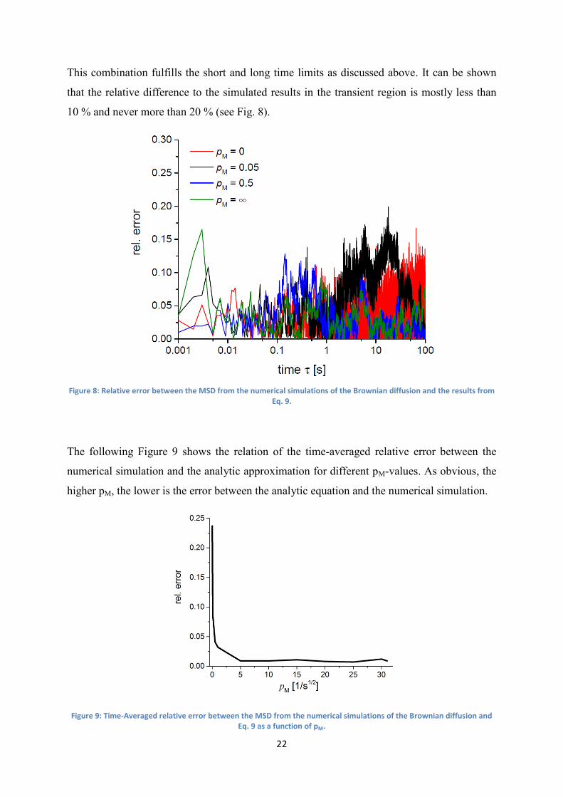
This combination fulfills the short and long time limits as discussed above. It can be shown

that the relative difference to the simulated results in the transient region is mostly less than

10 % and never more than 20 % (see Fig. 8).

Figure 8: Relative error between the MSD from the numerical simulations of the Brownian diffusion and the results from Eq. 9.

The following Figure 9 shows the relation of the time-averaged relative error between the

numerical simulation and the analytic approximation for different pM-values. As obvious, the

higher pM, the lower is the error between the analytic equation and the numerical simulation.

Figure 9: Time-Averaged relative error between the MSD from the numerical simulations of the Brownian diffusion and Eq. 9 as a function of pM.

23

So, our developed analytic approximation of the numerical simulation converges with higher

permeability pM, but also with a lower duration of the time step Δτ.

Our numerical simulation also confirms the following intuitive relation from the boundary

homogenization [38,44]: the smaller the permeability pM of the membranes, the lower Deff

will be, and vice versa. Naturally, the particle radius determines the free diffusion coefficient

D0(η, R) by Eq. 2 and the permeability through the membrane, the effective diffusion

coefficient Deff(pM(R),L,D0) respectively. Bigger particles cannot pass the apertures between

the cavities easily, thereby resulting in a reduced permeability, i.e., Deff becomes smaller.

Hence, the only essential parameters for MSD(τ) in Eq. 9 and in the simulations are D0 from

the unrestricted diffusion at short times, Deff from the restricted diffusion at long times, and L

as the cavity size [see Fig. 7(A)]. A direct consequence of the model is that the MSD ~ τα,

α < 1 appears only as a transient phenomenon, which should not be misinterpreted as

subdiffusion or abnormal diffusion (see Fig. 7(A) and Ref. [44]).

It is common to plot the MSD(τ) in a double logarithmic scale to visualize deviations from the

normal diffusive behavior. Berezhkovskii et al. provided in [40] a good method to

discriminate between anomalous diffusion (subdiffusion) and transient subdiffusive behavior

by calculating anomaly exponents α in three different ways. In case of anomalous diffusion, α

is constant and independent of the method of determination. In our study, we characterize the

transient "subdiffusive" behavior by determining a time-dependent anomaly exponent α(τ),

from the dimensionless logarithmic derivative of the MSD(τ). This is given as follows

[40,55,56]:

d

MSDd

MSDd

MSDd

log

log (10)

and shown in Fig. 7 (B).

Note that another possible characterization of the nonlinear MSD(τ) is given by a time

dependent diffusion coefficient MSD(τ) = 2D(τ)τ. Both characterizations are localized to a

specific time lag τ and do not represent the overall nature of the system.

In all experiments, the accessible time range is limited by both the frame rate of the camera

and the maximal recorded time interval that the diffusing particle is within the depth of field

of the microscope for detection, e.g., τ is between 0.05 and 5 s [11,14]. In Fig. 7, we used

various Deff and a reasonable interstitial fluid viscosity of η = 3.5 mPas, which is similar to

24

that of water. Hence, the predicted time range of transition ("subdiffusion") appears within the

typically experimental conditions.

The presented model focuses on a qualitative description, using only as few parameters as

possible. Therefore, we can neither cover the broad range of existing mucus variations nor the

various types of particle coatings. Using only three physical interpretable parameters, we can

reproduce the measured ”subdiffusive” behavior. However, the ”subdiffusion” reflected by a

MSD ~ τα, α < 1, is identified as a transient behavior. It naturally appears due to the

continuous transition from normal, unrestricted diffusion (MSD ~ τ) at short times to a

normal, restricted diffusion at long-time scales, longer distances respectively, caused by the

repeated confinement of the particles. The two limiting normal diffusion regimes are

quantized by the diffusion coefficients, D0 and Deff, respectively. The third necessary

parameter in the model is the mean cavity size L. The transition regime should not be

identified as anomalous diffusion in the sense of space-time scale invariant, continuous-time

random walks, or as a fractional Brownian motion [40]. Only one length scale is added to the

system, the mean cavity size L.

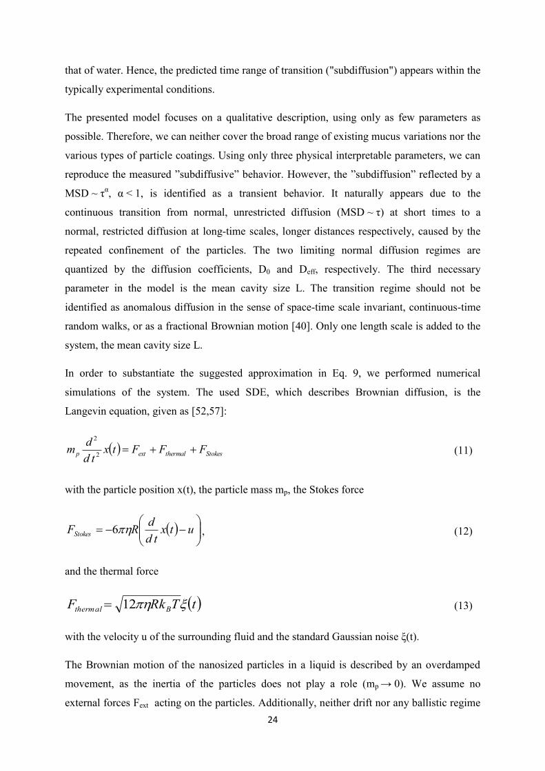
In order to substantiate the suggested approximation in Eq. 9, we performed numerical

simulations of the system. The used SDE, which describes Brownian diffusion, is the

Langevin equation, given as [52,57]:

Stokesthermalextp FFFtxtd

dm

2

2

(11)

with the particle position x(t), the particle mass mp, the Stokes force

utx

td

dRFStokes 6 , (12)

and the thermal force

tTkRF Bthermal 12 (13)

with the velocity u of the surrounding fluid and the standard Gaussian noise ξ(t).

The Brownian motion of the nanosized particles in a liquid is described by an overdamped

movement, as the inertia of the particles does not play a role (mp → 0). We assume no

external forces Fext acting on the particles. Additionally, neither drift nor any ballistic regime

25

will appear during the particle movement and we also neglect the velocity of the surrounded

fluid, as we assume the interstitial fluid to be static. Under these assumptions, the unrestricted

(free) motion of the particles at all times is then described by the massless Smoluchowski-

approximation of the Langevin equation [52,57]:

tDtxtd

d02 (14)

A very efficient way to simulate this stochastic equation at discrete times is given by the

Euler-Maruyama method [52,58-60], as follows:

1,,1;2 0

1

NkgDx

withxxx

k

kkk

(15)

where N is the maximum number of time steps and g ϵ N(0,1) is a Gaussian distributed

random number. We use a uniformly distributed initial position x0 ϵ [0,L].

In presence of reflecting walls or permeable membranes, the particle motion must comply

with the boundary conditions in each iteration. The treatment of diffusion through permeable

membranes is still a topic of current research. We adapt the algorithm, referred as the Robin

boundary condition, from [59,60] for partially reflecting and absorbing walls. The permeable

membranes in our simulations are described by a random reflecting and passing of the wall,

independent of the angle of impact. Hence, the iteration scheme from Eq. 15 has to be

modified. When the particle trace hits the membrane, the probability of reflection must

depend on the spatial resolution of the simulation, the duration of the discrete time step

respectively. It becomes clear that a shorter Δτ leads to a more fractional trajectory, and there

are more hits to an (imaginary) wall in the same time span. To preserve the ratio of

transmissions per unit time, the probability of reflection at each hit must be reduced.

According to [59,60], we introduced the reflection probability r:

Mpr 1 (16)

with the permeability pM ϵ [0,∞] of the membrane in units of s-1/2

. The iteration scheme in

Eq. 15 and the reflecting probability in Eq. 16 requires a sufficiently small Δτ to achieve

accurate statistical quantities, at least to preserve a r ϵ [0;1]. This requirement results in a

small time step Δτ, particular in the limiting case of pM → ∞, and consequently Deff → D0.

The modified iteration scheme is given as follows:

26

.

,,

1otherwisex

crossedismembraneaifrwithxxx

k

rk

kk (17)

The displacement of the particle for being reflected by the periodic membranes at x = jL,

j ϵ Z, is given as follows:

0,,mod2

0,,mod22,

kkk

kkk

rkxLxx

xLxLxx (18)

using the modulus function mod. The Δxk > 0 represents a particle motion from left to right

and Δxk < 0 is the reverse. For more details, please see the supplementary material. Some

exemplary trajectories in 2D are shown in Fig. 6(C). In this Figure, the x and y components of

each trajectory are two independent 1D simulations. The particles are mostly caged in the

current cavity, but they can also pass through the borders/membranes with a certain

probability 1-r.

In Figure 10 the relation between the permeability pM, respectively the reflection probability

r(pM), and the effective diffusion coefficient Deff(pM) is given. As shown, Deff increases with a

higher distance between the membranes L, in particular for low pM-values. Here, the

approximation at Deff = D0 is obvious for high pM-values, when the particles can move freely

without appearing permeable membranes, respectively with membranes, described by a

reflection probability of r = 0.

27

Figure 10: Calculated ratio Deff/D0 with D0 = 0.32 µm² s-1

(R = 100 nm, η = 7 mPas) as function of pM, respectively r, and various membrane distances L. A Δτ 1 ms was used in the numerical simulations of Brownian diffusion.

There is an approximation of the ratio Deff/D0 for pM → ∞ to a value of one and also an

approximation for pM → 0 to a value of zero. As obvious, the higher the distance between the

permeable membranes L, the lower is the needed pM to achieve a Deff = 0.

Similar to the analytical solution of MSDapp from Eq. 9, we developed a further analytic

approximation equation to yield the MSDanal of particles diffusing in an array of cavities, also

separated by permeable membranes. Contrary to the numerical simulations, which can be

described by Eq. 9, now, we keep the probability of a particle to pass the permeable

membrane to be constant for each time step in the numerical iteration scheme from Eq. 17 and

Eq. 18. However, to simulate this kind of diffusion by a stochastic Wiener process, we used

the same iteration scheme, but as already mentioned, with a constant instead of a random

permeation probability of a particle for each time step. The analytical solution to describe this

numerical iteration scheme, respectively to calculate the MSD, is hence given as:

021 DrMSDrMSD Lanal (19)

with the reflection probability, as described in Eq. 16. Henceforward, we name the numerical

simulation of particle diffusion, based on random permeation probabilities, respectively the

diffusion, described by Eq. 9, as Brownian diffusion. The diffusion, described by Eq. 19,

28

respectively the numerical simulation, based on constant permeation probabilities, will be

named as Fickian diffusion from this point onward. Latter can be easily compared with the

cell-window model, whereat the former diffusion model is comparable to the cell-array model

(see section 4.3.2).

Figure 11 shows the analytical solution for the MSDanal, as described in Eq. 19, and the

corresponding anomaly exponent α, which is the slope of the MSD-curve in a double

logarithmic plot. The data from numerical simulations of the Fickian diffusion are shown as

symbols.

Figure 11: (A) Calculated MSD from particles with a diameter of 200 nm in mucus using a membrane distance of L = 0.35 µm and D0 = 0.65 µm²/s for various permeability of the membranes pM and the belonging Deff in the legend. Data

from numerical simulations of Fickian diffusion are shown as symbols (Δτ = 1 ms), and are from an analytic approximation using Eq. 19 as lines. (B) The calculated anomaly exponent α to MSD(τ) ~ τ

α using Eq. 10 with the same

legend as in (A).

The combination in Eq. 19 again fulfills the short and long time limits as already discussed,

and shows that the relative difference to the simulated results in the transient region is mostly

less than 15 % and we have never found the deviation to be more than 35 % (see Fig. 12).

29

Figure 12: Relative error between the MSD from the numerical simulations of the Fickian diffusion and the results from Eq. 19.

The following Figure 13 shows the relation of the time-averaged relative error between the

numerical simulation and the analytic approximation from Eq. 19 for different pM-values.

Since here, the dependency is not that obvious as in Fig. 9, however, the higher pM, the lower

is the error between the analytic equation and the numerical simulation.

Figure 13: Averaged relative error between the MSD from the numerical simulations of the Fickian diffusion and Eq. 19 as a function of pM.

Again, our developed analytic approximation of this numerical simulation converges with

higher permeability pM and a lower duration of the time step Δτ.

Surprisingly, when the ratio between Deff and D0 is plotted against different values of pM with

a distance L of 100 nm, 300 nm and 500 nm (see Fig. 14), for the Fickian diffusion we get a

completely different shape of the curve, compared to the Brownian diffusion (see Fig. 10).

30

Here, the approximation at Deff = 0 is obvious for low pM-values, when the particle movement

is almost totally restricted (r = 1).

Figure 14: Calculated ratio Deff/D0 with D0 = 0.32 µm² s-1

(R = 100 nm, η = 7 mPas) as function of pM, respectively r, and various membrane distances L. A Δτ 1 ms was used in the numerical simulations (Fickian diffusion).

As obvious, the pM-value for Deff = 0 depends also on the distance between the permeable

membranes L. So, the Brownian diffusion converges to a Deff = D0 for high permeabilities,

whereas the Fickian diffusion converges to a Deff = 0 for low permeabilities.

As already mentioned, this analytical equation (Eq. 19) does not describe the Brownian, but

the Fickian diffusion of particles within confined geometries. So, we developed analytical

solutions for both numerical simulations and in the next section, we will compare the

Brownian diffusion with the Fickian diffusion. Additionally, we will also compare the

simulated Fickian and Brownian diffusion with experimental studies.

The numerical simulation of long trajectories opens up the possibility to determine the

relation between the permeability pM used in the simulation and the ratio of effective to free

diffusivity Deff = D0. For various fixed lattice constants L, see Fig. 10, respectively Fig. 14. As

expected, the relation is strictly increasing, nonlinear and saturates in unity for large

permeability, respectively in zero for low permeability. A general analytic derivation of this

relation is still an open question [59,60]. Note that the pM is neither in direct relation to the

31

permeability P nor the trapping rate κ in [26,27,44]; the physical units are different. Our

simulations are also different from those former approaches [26,27,44], due to the explicit

usage of permeable membranes instead of a 2D or 3D simulation of standard Brownian

motion in a cubic lattice with apertures of fixed size and reflecting walls.

Finally, the presented model predicts a transient "subdiffusive" behavior in the experimentally

accessible time range between 0.05 and 5 s for realistic parameter assumptions. For instance,

for a particle diameter of 200 nm, a cavity extension of L = 350 nm, and using a permeability

pM = 0.05, this results in an effective mucus viscosity of 100 times more as it of the interstitial

fluid (see bullets and black line in Fig. 7 and Fig. 11, respectively). A transient ”subdiffusive”

time range also remains for other particle diameters due to the following conclusion: smaller

particles belong to a larger D0 (see Eq. 2), and result in a larger expected Deff. Hence, the

MSD(τ) curve will shift upwards in the double logarithmic plot and for fixed L, the time

range with ”subdiffusion” will shift slightly to smaller values. The opposite is in the case for

bigger particles. Hence, a transient ”subdiffusive” behavior is predicted for any particle

diameter if Deff < D0. However, if the particles become very small, as they can pass the

membranes/the scaffold structure very easily (pM will increase), Deff will be in the order of

magnitude of D0 and the ”subharmonic” region will disappear.

4.1.3 Results & Discussion

In this section, model predictions with measured MSD(τ) are compared by adapting the

required parameters to obtain a good visual agreement. The physical meaning of our results

are discussed and they are compared with independent measurements, if available. There are

results from other theoretical studies, where a similar shape of the MSD-curves and anomaly

exponent α, as shown in Fig. 7 and Fig. 11, were predicted , but using other assumptions and

models [27,40-42,44,48,50,55]). We used particle tracking data from uncoated, polystyrene

(PS) particles in human sputum from cystic fibrosis (CF) patients [14] and from coated

PEGylated, as well as carboxylated polystyrene particles in pulmonary mucus from humans

without lung disease [11]. A comprehensive model with including inter-particle and particle-

boundary interactions can be found in [50], where the simulated results and the observed

transient ”subdiffusive” behavior are compared with experimental studies.

32

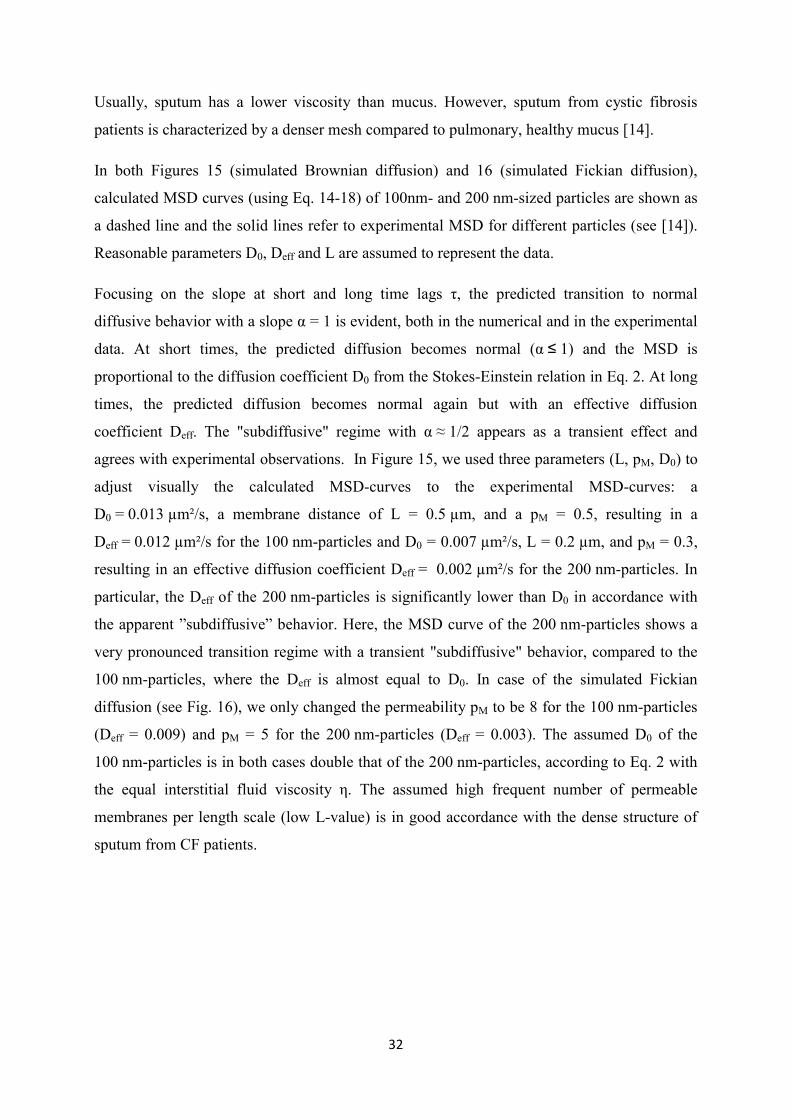
Usually, sputum has a lower viscosity than mucus. However, sputum from cystic fibrosis

patients is characterized by a denser mesh compared to pulmonary, healthy mucus [14].

In both Figures 15 (simulated Brownian diffusion) and 16 (simulated Fickian diffusion),

calculated MSD curves (using Eq. 14-18) of 100nm- and 200 nm-sized particles are shown as

a dashed line and the solid lines refer to experimental MSD for different particles (see [14]).

Reasonable parameters D0, Deff and L are assumed to represent the data.

Focusing on the slope at short and long time lags τ, the predicted transition to normal

diffusive behavior with a slope α = 1 is evident, both in the numerical and in the experimental

data. At short times, the predicted diffusion becomes normal (α ≤ 1) and the MSD is

proportional to the diffusion coefficient D0 from the Stokes-Einstein relation in Eq. 2. At long

times, the predicted diffusion becomes normal again but with an effective diffusion

coefficient Deff. The "subdiffusive" regime with α ≈ 1/2 appears as a transient effect and

agrees with experimental observations. In Figure 15, we used three parameters (L, pM, D0) to

adjust visually the calculated MSD-curves to the experimental MSD-curves: a

D0 = 0.013 µm²/s, a membrane distance of L = 0.5 µm, and a pM = 0.5, resulting in a

Deff = 0.012 µm²/s for the 100 nm-particles and D0 = 0.007 µm²/s, L = 0.2 µm, and pM = 0.3,

resulting in an effective diffusion coefficient Deff = 0.002 µm²/s for the 200 nm-particles. In

particular, the Deff of the 200 nm-particles is significantly lower than D0 in accordance with

the apparent ”subdiffusive” behavior. Here, the MSD curve of the 200 nm-particles shows a

very pronounced transition regime with a transient "subdiffusive" behavior, compared to the

100 nm-particles, where the Deff is almost equal to D0. In case of the simulated Fickian

diffusion (see Fig. 16), we only changed the permeability pM to be 8 for the 100 nm-particles

(Deff = 0.009) and pM = 5 for the 200 nm-particles (Deff = 0.003). The assumed D0 of the

100 nm-particles is in both cases double that of the 200 nm-particles, according to Eq. 2 with

the equal interstitial fluid viscosity η. The assumed high frequent number of permeable

membranes per length scale (low L-value) is in good accordance with the dense structure of

sputum from CF patients.

33

Figure 15: Comparison of experimental data and the calculated MSD for 100 nm- and 200 nm-particles, indicated as a dashed and a straight line, respectively. A membrane distance L = 0.5 µm, a diffusion coefficient D0 = 0.013 µm²/s, and a permeability pM = 0.5 were assumed for the 100 nm-particles. A membrane distance L = 0.2 µm, a diffusion coefficient

D0 = 0.007 µm²/s, and a permeability pM = 0.3 were assumed for the 200 nm-particles. These assumptions result in a ratio of Deff/D0 = 0.88 and Deff/D0 = 0.35 for the particles with a diameter of 100 and 200 nm, respectively. In the background, a figure taken from [14] with experimental data for polystyrene particles in human sputum from CF patients (solid lines) is

shown. The transient time regime of "subdiffusion" is marked.

Figure 16: Comparison of experimental data and the calculated MSD for 100 nm- and 200 nm-particles, indicated as a dashed and a straight line, respectively. A membrane distance L = 0.5 µm, a diffusion coefficient D0 = 0.013 µm²/s, and a

permeability pM = 8 were assumed for the 100 nm-particles. A membrane distance L = 0.2 µm, a diffusion coefficient D0 = 0.007 µm²/s, and a permeability pM = 5 were assumed for the 200 nm-particles. These assumptions result in a ratio of Deff/D0 = 0.7 and Deff/D0 = 0.45 for the particles with a diameter of 100 and 200 nm, respectively. In the background, a figure taken from [14] with experimental data for polystyrene particles in human sputum from CF patients (solid lines) is

shown. The transient time regime of "subdiffusion" is marked.

Note that according to the isotropy of the model, the 2D- and 3D-MSD is given by the double

and triple of the predicted 1D-MSD. In Fig. 15 and Fig. 16 we show, that our simulated 3D-

MSD data are well in line with experimental data as reported in [14].

34

Due to the less dense mesh in healthy mucus, compared to mucus from CF patients, also the

diffusivity of 500 nm particles is discussed in the following paragraphs. In sputum from CF

patients, these particles are totally trapped, but in healthy mucus, the mean pore size is high

enough to allow bigger particles to diffuse through the mucus layer. However, the time, which

is needed to pass this layer is significantly higher than that for smaller particles (see

section 4.2.3).

In each of the Figures 17 (simulated Brownian diffusion) and 18 (simulated Fickian

diffusion), three calculated MSDs are compared with the experimental MSD of different sized

carboxylated particles in pulmonary mucus from humans without lung disease [11].

Reasonable values of the parameters D0, Deff and L are assumed to represent the data. The

different offset in the MSD for the various sized particles is simply due to the different D0

(see Eq. 2) and the equal assumed interstitial fluid viscosity η. In Figure 17, we assumed the

following parameters (D0, pM, L) to adjust visually the calculated MSD-curves to the

experimental MSD-curves of particles with a size of 100 nm (straight black line), 200 nm

(grey dashed line), and 500 nm (grey dotted line), respectively: (0.017 µm²/s, 0.5, 0.5 µm);

(0.004 µm²/s, 0.1, 0.15 µm); (0.002 µm²/s, 0.05, 0.15 µm). The resulting Deff are 0.007 µm²/s,

0.0003 µm²/s, and 0.0002 µm²/s, respectively. In case of the simulated Fickian diffusion (see

Fig. 18), we changed the permeability pM to be 5 for the 100 nm-particles (Deff = 0.003),

pM = 3 for the 200 nm-particles (Deff = 0.0003), and pM = 1.5 for the 500 nm-particles

(Deff = 0.0001).

Figure 17: Comparison of calculated MSD for various parameters as dash-dotted lines and measured data as background image from [11]. A membrane distance L = 0.5 µm for the 100nm-particles and L = 0.15 µm for the 200nm- and 500nm-

particles was assumed. The parameters of (D0, Deff/D0, pM) are given as (top to bottom) (0.017 µm²/s, 0.4, 0.5), (0.004 µm²/s, 0.09, 0.1), (0.002 µm²/s, 0.09, 0.05).

35

Figure 18: Comparison of calculated MSD for various parameters as dash-dotted lines and measured data as background image from [11]. A membrane distance L = 0.5 µm for the 100nm-particles and L = 0.15 µm for the 200nm- and 500nm-

particles was assumed. The parameters of (D0, Deff/D0, pM) are given as (top to bottom) (0.017 µm²/s, 0.18, 5), (0.004 µm²/s, 0.08, 3), (0.002 µm²/s, 0.05, 1.5).

If the particles are coated by PEG and are thus neutral (uncharged), less adherent or repulsive

interaction between particles and mucus is observed [1,2]. Hence, the effective diffusion

coefficient Deff increases and becomes comparable to D0, and consequently the transient

"subdiffusive" regime becomes less pronounced. This is the topic of the following paragraph.

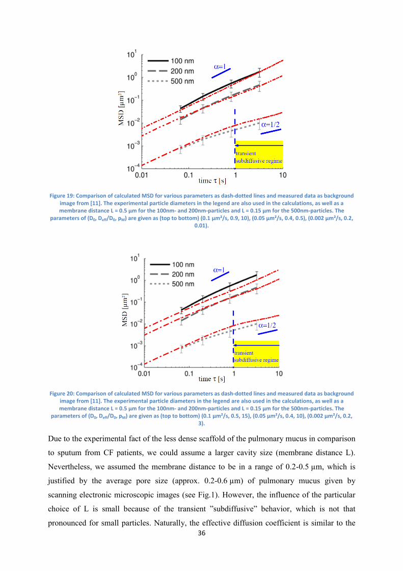
In Figure 19 (simulated Brownian diffusion) and Figure 20 (simulated Fickian diffusion),

three calculated MSDs are compared with the experimental MSD of different sized

PEGylated particles in pulmonary mucus from humans without lung disease [11]. Reasonable

values of D0, Deff and L are assumed to represent the data. Again, the different offset in the

MSD for the 100nm- and 200nm-particles is due to the different D0 (see Eq. 2). This is

because of the same assumed interstitial fluid viscosity η. We assumed a membrane distance

of L = 500 nm for the 100 nm- and 200 nm-particles, a L = 150 nm for the 500 nm-particles,

and the following values of D0 and pM: 0.1 µm²/s and 10 for the 100 nm-particles, 0.05 µm²/s

and 0.5 for the 200 nm-particles, and 0.002 µm²/s and 0.01 for the 500nm-particles; the

resulting Deff are 0.09 µm²/s, 0.02 µm²/s, and 0.0005 µm²/s, respectively. In case of the

simulated Fickian diffusion (see Fig. 20), we only changed the permeability pM to be 15 for

the 100 nm-particles (Deff = 0.04), pM = 10 for the 200 nm-particles (Deff = 0.02), and pM = 3

for the 500 nm-particles (Deff = 0.0004).

36

Figure 19: Comparison of calculated MSD for various parameters as dash-dotted lines and measured data as background image from [11]. The experimental particle diameters in the legend are also used in the calculations, as well as a membrane distance L = 0.5 µm for the 100nm- and 200nm-particles and L = 0.15 µm for the 500nm-particles. The

parameters of (D0, Deff/D0, pM) are given as (top to bottom) (0.1 µm²/s, 0.9, 10), (0.05 µm²/s, 0.4, 0.5), (0.002 µm²/s, 0.2, 0.01).

Figure 20: Comparison of calculated MSD for various parameters as dash-dotted lines and measured data as background image from [11]. The experimental particle diameters in the legend are also used in the calculations, as well as a membrane distance L = 0.5 µm for the 100nm- and 200nm-particles and L = 0.15 µm for the 500nm-particles. The

parameters of (D0, Deff/D0, pM) are given as (top to bottom) (0.1 µm²/s, 0.5, 15), (0.05 µm²/s, 0.4, 10), (0.002 µm²/s, 0.2, 3).

Due to the experimental fact of the less dense scaffold of the pulmonary mucus in comparison

to sputum from CF patients, we could assume a larger cavity size (membrane distance L).

Nevertheless, we assumed the membrane distance to be in a range of 0.2-0.5 µm, which is

justified by the average pore size (approx. 0.2-0.6 µm) of pulmonary mucus given by

scanning electronic microscopic images (see Fig.1). However, the influence of the particular

choice of L is small because of the transient ”subdiffusive” behavior, which is not that

pronounced for small particles. Naturally, the effective diffusion coefficient is similar to the

37

D0 from the unrestricted motion. It seems there is only a minor influence on the diffusion of

the small particles due to the membranes.

The situation is different for the MSD curves of bigger particles. The transient ”subharmonic”

behavior becomes significantly visible and the influence of the permeable membranes

becomes dominant. For the simulations of the diffusion of bigger particles, we assumed a

larger viscosity η as for the smaller particles. Consequently, D0 and Deff are smaller as

expected from the indicated particle size (see Eq. 2). This is in accordance with the

experimental observation: a larger apparent viscosity of the mucus at small time scales due to

a particle size comparable with the cavity size because of increased steric obstruction [3]. The

finite sized particles are affected by the scaffold structure at any time scale and the

assumption of point like tracer particles in the model is not more justified. In addition, we also

assume a smaller distance between the membranes, respectively, the mean cavity size is as

much smaller as the particle diameter. This assumption is justified by the average pore size

(approx. 0.05-0.2 µm) of pulmonary mucus given by scanning electronic microscopic images

(see Fig.1), where the pore sizes are extremely small, compared to the particle size. Despite

the fact that, the particles will be trapped in the mucus mesh, because the pore size is as much

smaller as the particle size, we assumed a L < 2R in our simulations. Nevertheless, in our

model, L as mean cavity size is the first order approximation, and the physical meaning

should not be overinterpreted in our simplified model, particularly when our particles are

assumed as non-extended tracers. Even though, the presented model does not consider

chemical or electrostatic effects. However, we are able to reproduce the experimental data of

either uncoated (charged) or coated (uncharged) particles, according to the Figures 15-20.

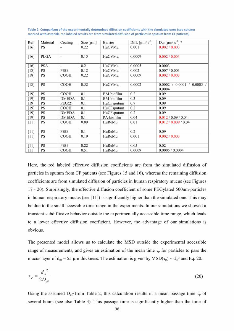
In Table 2 the computed Deff (*) from our simulations (see Figures 15-20) are compared with

the corresponding data from other experiments, as shown in Table 1. Only the best fitting data

from these studies are presented in comparison with our results.

38

Table 2: Comparison of the experimentally determined diffusion coefficients with the simulated ones (see column marked with asterisk, red labeled results are from simulated diffusion of particles in sputum from CF patients).

Ref. Material Coating Size [µm] Barrier Diff. [µm² s-1

] Deff [µm² s-1

] *

[16] PS - 0.22 HuCVMu 0.001 0.002 / 0.003

[16] PLGA - 0.15 HuCVMu 0.0009 0.002 / 0.003

[16] PSA - 0.2 HuCVMu 0.0005 0.0003

[18] PS PEG 0.12 HuCVMu 0.002 0.007 / 0.003

[18] PS COOH 0.22 HuCVMu 0.0009 0.002 / 0.003

[18] PS COOH 0.52 HuCVMu 0.0002 0.0002 / 0.0001 / 0.0005 /

0.0004

[19] PS COOH 0.1 BM-biofilm 0.2 0.09

[19] PS DMEDA 0.1 BM-biofilm 0.3 0.09

[19] PS PEG(2) 0.1 HuCFsputum 0.7 0.09

[19] PS COOH 0.1 HuCFsputum 0.2 0.09

[19] PS DMEDA 0.1 HuCFsputum 0.2 0.09

[19] PS DMEDA 0.1 PA-biofilm 0.04 0.012 / 0.09 / 0.04

[11] PS COOH 0.09 HuReMu 0.01 0.012 / 0.009 / 0.04

[11] PS PEG 0.1 HuReMu 0.2 0.09

[11] PS COOH 0.19 HuReMu 0.001 0.002 / 0.003

[11] PS PEG 0.22 HuReMu 0.05 0.02

[11] PS COOH 0.51 HuReMu 0.0009 0.0005 / 0.0004

Here, the red labeled effective diffusion coefficients are from the simulated diffusion of

particles in sputum from CF patients (see Figures 15 and 16), whereas the remaining diffusion

coefficients are from simulated diffusion of particles in human respiratory mucus (see Figures

17 - 20). Surprisingly, the effective diffusion coefficient of some PEGylated 500nm-particles

in human respiratory mucus (see [11]) is significantly higher than the simulated one. This may

be due to the small accessible time range in the experiments. In our simulations we showed a

transient subdiffusive behavior outside the experimentally accessible time range, which leads

to a lower effective diffusion coefficient. However, the advantage of our simulations is

obvious.

The presented model allows us to calculate the MSD outside the experimental accessible

range of measurements, and gives an estimation of the mean time τp for particles to pass the

mucus layer of dm = 55 µm thickness. The estimation is given by MSD(τp) ~ dm² and Eq. 20.

eff

mp

D

d

2

2

(20)

Using the assumed Deff from Table 2, this calculation results in a mean passage time τp of

several hours (see also Table 3). This passage time is significantly higher than the time of

39

τMC = 15 min required to renew the layer, given by the mucociliary clearance [4,7,10]. Even

for a free Brownian motion (MSD ~ D0) of 200 nm-particles in a fluid with η = 4 mPas, the

passage time is approximately one hour. It can be summarized that particles with a diameter

lower than 40 nm are able to pass through the mucus layer of d = 55 µm thickness (with a

viscosity of the interstitial fluid of η = 7 mPas) within a mucus turnover time of 15 min. In

chapter 4.2, we will calculate the mean passage time and the percentage of particles, passing

the mucus layer after a certain specified time range, for each presented experiment,

respectively simulation, from Fig. 15-20.

40

4.2 A model to predict particle diffusion in mucus for short and long time limits

4.2.1 Introduction

Mucus protects our body from environmental influences as it is a biological barrier for foreign

substances to the epithelial cell layer, e.g. in the lung. For particle-based drug delivery

systems, the mucus layer generates an extra challenge as drug-loaded particles must overcome

this layer. Thus, solid drug delivery systems and the penetration of particulate matter, such as

viruses, bacteria, and dust are affected. Mucus is a complex, heterogeneous polymer-scaffold

with viscoelastic properties, which consists of mainly mucins and of a low viscous interstitial

fluid (see Fig. 1). However, the main component of mucus is the interstitial space, which

essentially is filled by a fluid with a viscosity, similar to that of water, in the range of a few

mPas. To avoid systemic side effects by the therapy of bronchial diseases, e.g. cystic fibrosis,

local applications of drug delivery systems are preferable. In the bronchial regions of the lung,

pulmonary mucus is present, where its function is the clearance of particulate xenobiotics,

mucosal insults, water balance, ion transport, and ion regulation. Some functionalized and

non-toxic nanocarriers, loaded with novel pharmaceuticals, can overcome this biological

barrier after being inhaled. Inspired from viruses, nanosized particles with neutrally charged

coatings such as PEG can efficiently penetrate the mucus layer in contrast to charged

particles. Particularly, the studies from Lai et al., Suk et al., Suh et al. and Schuster et al.

showed an enhanced penetration of PEGylated particles, compared to conventionally

uncoated or carboxylated particles. For comparison, generally the mean squared displacement

as a function of the time lag (MSD(τ)) is measured by particle tracking experiments [1-12,14].

So far, the accessible time range in particle tracking experiments is limited by both the frame

rate of the camera and the maximal recorded time interval that the diffusing particle is within

the depth of field of the microscope for detection. Therefore, the particle diffusion for very

short (τ < 0.01 - 0.05 s) and very long (τ > 5 - 10 s) time periods cannot be determined. Due to

the fact that in many experiments, the transition from the transient ”subdiffusive” regime -

which is defined by a transient decrease of the slope of the MSD curve- to the normal

diffusion regime is outside the accessible time range, the diffusion is falsely interpreted as an

anomalous diffusion (subdiffusion). To predict the diffusivity of particles in confined

geometries -such as mucus- in short and long time limits, and also the observed transient

”subdiffusive” behavior, in the prior section we introduced a model, based on permeable

membranes and an effective diffusion coefficient Deff, which is lower than the diffusion

41

coefficient D0 from the Stokes-Einstein relation. This model allows to simulate the MSD of

particles in the short and long time limit. In between these limits, a transient ”subdiffusive”

regime appears, which is also observed in some experimental studies [11, 14]. So, instead of

assuming a totally restricted subdiffusion, we showed the diffusion in confined geometries to

be partially restricted with a normal diffusive behavior for short and long times, however, the

diffusion is described by the diffusion coefficient from the Stokes-Einstein relation D0 and by

an effective diffusion coefficient Deff, respectively.

4.2.2 Model & experimental findings

The Figure 6 suggests the model of mucus, which is based on a porous structure of Newtonian

fluid-filled random-sized cavities with apertures of various sizes. The system has been

simplified to a simple cubic lattice of cavities with connecting apertures and is characterized

by a mean cavity extension L and a mean aperture diameter [see Fig. 6 (A)]. L is the edge size

of one cavity in the cubic lattice, respectively the distance between the cavity interfaces. The

shown anisotropic scaffold structure in Fig. 6 (A) is condensed by the ”boundary

homogenization” method assuming permeable membranes in all spatial directions, and

quantified by a certain permeability of the membranes pM for the particles [see Fig. 6 (B) and

(C)]. The resulting three-dimensional isotropic system is then further reduced to a one-

dimensional system. Despite the numerical iteration scheme, we showed also an analytic

approximation, which is the appropriate superposition of the analytic solutions for free and

trapped particle diffusion. Sanders et al. showed a microscopic image of sputum from cystic

fibrosis (CF) patients, which illustrate the more dense structure of this sputum [13], compared

to pulmonary mucus from healthy humans (see Figure 1). Using only the three physical

interpretable parameters L, D0, and Deff(pM), the measured ”subdiffusive” behavior from

particle tracking experiments can be reproduced. The ”subdiffusive” behavior appears due to

the continuous transition from normal, unrestricted diffusion MSD ~ τ at short times to a

normal, restricted diffusion at long-time scales, longer distances respectively. The two

limiting normal diffusion regimes are quantized by the diffusion coefficients, D0 and Deff,

respectively. The permeability of the membranes is characterized by pM, affecting Deff. The

third necessary parameter in the model is the mean cavity size L as the only length scale in the

system. So, as we assume different values of the permeabilities pM and the mean cavity size L,

we are able to reproduce the experimental data and predict the diffusive behavior of either

42

uncoated (charged) or coated (uncharged) particles in mucus with different properties for each

time scale.

There exist several studies on the particle diffusion in mucus, for instance the investigations

by Suh et al. or Schuster et al. [11,14]. Unfortunately, in these studies, the accessible time

range is very short (approx. 2-3 decades) and they cannot determine the probability density

function (pdf) of the particle displacement in the mucus layer. The latter is important to know,

as it provides the percentage of particles, which are passing a specified thickness after a

certain time range. Contrary to the pdf, the mean squared displacement (MSD) provides only

the mean passage time of one particle. For this reason, we assumed the three essential

parameters Deff(pM), D0, and L to predict the short and long time diffusion, e.g. the MSD over

minimum 5 decades, and to determine the pdf.

In the prior section, we presented the experimental studies to determine the diffusivity of

particles in pulmonary mucus and finally we calculated the MSD and the effective diffusion

coefficient Deff. By assuming specific values for the distance between the permeable

membranes L and the permeability of these membranes pM, we simulated the particle

diffusion in mucus in the short and long time limits. We also predicted the effective diffusion

coefficient, assuming different values of pM and L, which are related to the observed structure

and pore size distribution of mucus (see Figure 1) and the particle properties. So, the cavity

size L is related to the mucus structure, e.g. the pore size, whereas the permeability pM is

affected by the physical and chemical properties of the particles and the mucus. Additionally,

in the posterior section we will compute the probability density function of the particle

position within the confined geometry (based on repeated permeable membranes in one

dimension). Consequently, by assuming different values of L and pM, affecting Deff, we are

able to simulate the particle diffusion in mucus (MSD) and to predict the mean passage time

of particles to pass a defined mucus layer thickness, as well as to determine the percentage of

particles, passing the mucus layer within a specified time range.

43


The parameters of L, D0, and pM, respectively Deff, from the MSD-calculations in Figure 15-

20 are also used to simulate the pdf of the particle displacement after 100 s of Brownian and

Fickian diffusion in sputum from CF patients, which is shown in Figure 21 and 22,

respectively. The pdf is helpful to calculate the percentage of particles passing a specific

mucus layer with a certain thickness.

Figure 21: Calculated pdf for various parameters with particle diameters of 100 nm (red solid line) and 200 nm (blue dashed line), as well as a membrane distance L = 0.5 µm for the 100nm-particles and L = 0.2 µm for 200nm-particles. The

parameters of D0, Deff/D0, pM are given as (top to bottom) (0.013 µm²/s, 0.88, 0.5), (0.007 µm²/s, 0.35, 0.3).

Figure 22: Calculated pdf for various parameters with particle diameters of 100 nm (red solid line) and 200 nm (blue dashed line), as well as a membrane distance L = 0.5 µm for the 100nm-particles and L = 0.2 µm for 200nm-particles. The

parameters of D0, Deff/D0, pM are given as (top to bottom) (0.013 µm²/s, 0.7, 8), (0.007 µm²/s, 0.45, 5)

44

We could show that, 50% and 0.03% of the 100nm-particles overcome a distance of 1µm and

5 µm, respectively, after 100 s. Even 20% of the 200nm-particles overcome a distance of

1 µm within this time. In case of Fickian diffusion (Figure 22), 16% and 0.12% of the 100nm-

particles overcome a distance of 1µm and 5 µm, respectively, after 100 s. 7% of the 200nm-

particles overcome a distance of 1 µm within this time. Surprisingly, a higher number of

particles overcome a distance of 5 µm by Fickian diffusion, compared to Brownian diffusion,

whereas less particles overcome a distance of 1 µm by Fickian diffusion.

The parameters from the simulation of the MSD of carboxylated and PEGylated particles,

diffusing in pulmonary mucus are used to simulate the pdf of the displacement of these

particles after 100 s. The results are shown in Figure 23 and Figure 24 for the Brownian and

Fickian diffusion of carboxylated particles, respectively, and in Figure 25 and Figure 26 for

the Brownian and Fickian diffusion of PEGylated particles, respectively. The pdf allows to

calculate the percentage of particles passing a mucus layer with a thickness of 1 µm and

5 µm.

Figure 23: Calculated pdf for various parameters with carboxylated particle diameters of 100 nm (red solid line), 200 nm (blue dashed line), and 500 nm (black dash-dotted line) as well as a membrane distance L = 0.5 µm for the 100nm-

particles and L = 0.15 µm for 200nm- and 500nm-particles. The parameters of D0, Deff/D0, pM are given as (top to bottom) (0.017 µm²/s, 0.4, 0.5), (0.004 µm²/s, 0.09, 0.1), (0.002 µm²/s, 0.09, 0.05).

45

Figure 24: Calculated pdf for various parameters with carboxylated particle diameters of 100 nm (red solid line), 200 nm (blue dashed line), and 500 nm (black dash-dotted line) as well as a membrane distance L = 0.5 µm for the 100nm-

particles and L = 0.15 µm for 200nm- and 500nm-particles. The parameters of D0, Deff/D0, pM are given as (top to bottom) (0.017 µm²/s, 0.18, 5), (0.004 µm²/s, 0.08, 3), (0.002 µm²/s, 0.05, 1.5).

We show that, after a carboxylation of particles, only 54% and 0.13% of the 100nm-particles

overcome a distance of 1 µm and 5 µm, respectively, after 100 s. Compared to the PEGylated

particles (see Figures 25 and 26), due to the charged coating (COOH), less (only 2%) of the

200nm-particles overcome a distance of 1 µm after 100 s. However, even 0.03% of the

500nm-particles overcome a distance of 1 µm within this time. In case of Fickian diffusion

(Figure 24), 11% and 0.23% of the carboxylated 100nm-particles overcome a distance of

1 µm and 5 µm, respectively, after 100 s. Similar to Brownian diffusion, only 3% of the

200nm-particles overcome a distance of 1 µm after 100 s, whereas significantly more 500nm-

particles (0.9 %) overcome a distance of 1 µm within this time. As it is obvious for the

uncoated particles in CF sputum (Figures 21 and 22), also a higher number of coated particles

overcome a distance of 5 µm by Fickian diffusion, compared to Brownian diffusion, whereas

less particles overcome a distance of 1 µm by Fickian diffusion.

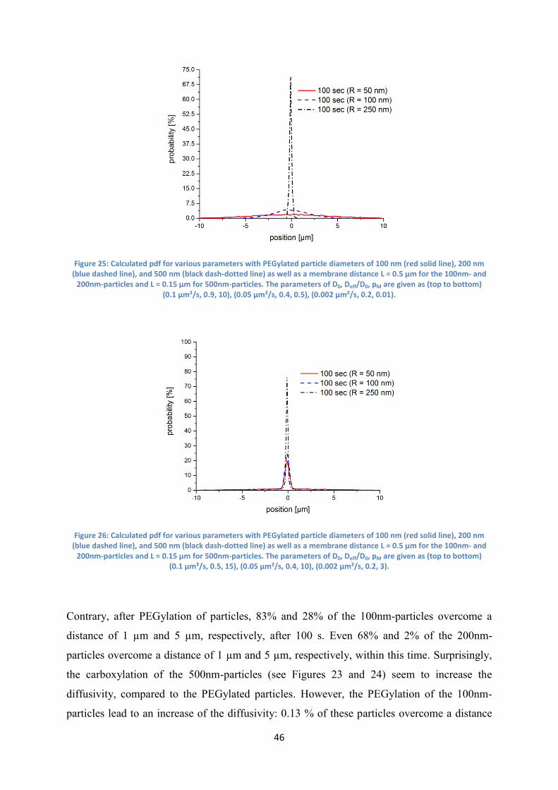
46

Figure 25: Calculated pdf for various parameters with PEGylated particle diameters of 100 nm (red solid line), 200 nm (blue dashed line), and 500 nm (black dash-dotted line) as well as a membrane distance L = 0.5 µm for the 100nm- and

200nm-particles and L = 0.15 µm for 500nm-particles. The parameters of D0, Deff/D0, pM are given as (top to bottom) (0.1 µm²/s, 0.9, 10), (0.05 µm²/s, 0.4, 0.5), (0.002 µm²/s, 0.2, 0.01).

Figure 26: Calculated pdf for various parameters with PEGylated particle diameters of 100 nm (red solid line), 200 nm (blue dashed line), and 500 nm (black dash-dotted line) as well as a membrane distance L = 0.5 µm for the 100nm- and

200nm-particles and L = 0.15 µm for 500nm-particles. The parameters of D0, Deff/D0, pM are given as (top to bottom) (0.1 µm²/s, 0.5, 15), (0.05 µm²/s, 0.4, 10), (0.002 µm²/s, 0.2, 3).

Contrary, after PEGylation of particles, 83% and 28% of the 100nm-particles overcome a

distance of 1 µm and 5 µm, respectively, after 100 s. Even 68% and 2% of the 200nm-

particles overcome a distance of 1 µm and 5 µm, respectively, within this time. Surprisingly,

the carboxylation of the 500nm-particles (see Figures 23 and 24) seem to increase the

diffusivity, compared to the PEGylated particles. However, the PEGylation of the 100nm-

particles lead to an increase of the diffusivity: 0.13 % of these particles overcome a distance

47

of 10 µm after 100 seconds. In case of Fickian diffusion (Figure 26), 39% and 14% of the

100nm-particles overcome a distance of 1 µm and 5 µm, respectively, after 100 s. 25% and

5% of the 200nm-particles overcome a distance of 1 µm and 5 µm, respectively, within this

time. Also for the Fickian diffusion, the PEGylation of particles increases the diffusivity (4 %

of the 500nm-particles overcome a distance of 1 µm and 0.08 % of the 100nm-particles even

overcome a distance of 10 µm after 100 seconds), compared to a carboxylation.

Finally, we are able to estimate the mean passage time τp for particles to pass the mucus layer

of dm = 55 μm thickness, which is given by Eq. 20. We used the Deff from the previously

mentioned simulations and some normal diffusion coefficients D0 to estimate the mean

passage time for different sized particles with various coatings, diffusing in healthy mucus

and sputum from CF patients. In Table 3, all mean passage times are presented.

Table 3:Summary of the diffusion coefficients, the mean passage times (to overcome a distance of 55 µm), the simulation parameters, the mucus- and the particle properties of the experiments and simulations, which are shown in the Figures 15-26 (the rows in red are from simulated Fickian diffusion).

D0 [µm²/s] Deff [µm²/s] Mucus Particle

size [µm]

Particle

coating

τp(D0) τp(Deff)

R = 50 nm

η = 1 mPas

4.54 - Fluid 0.1 - 5.6 min -

R = 50 nm

η = 10 mPas

0.45 - Fluid 0.1 - 55.5 min -

R = 100 nm

η = 10 mPas

0.23 - Fluid 0.2 - 111 min -

R = 250 nm

η = 10 mPas

0.09 - Fluid 0.5 - 278 min -

pM = 0.01

L = 0.15 µm

0.002 0.0005 Pulmon. 0.5 PEG 210 h 840 h

pM = 0.05

L = 0.15 µm

0.002 0.0002 Pulmon. 0.5 COOH 210 h 2100 h

pM = 0.1

L = 0.15 µm

0.004 0.0003 Pulmon. 0.2 COOH 105 h 1400 h

pM = 0.3

L = 0.2 µm

0.007 0.002 CF 0.2 - 60 h 210 h

pM = 0.5

L = 0.5 µm

0.013 0.012 CF 0.1 - 32 h 35 h

pM = 0.5

L = 0.5 µm

0.017 0.007 Pulmon. 0.1 COOH 25 h 60 h

48

pM = 0.5

L = 0.5 µm

0.05 0.02 Pulmon. 0.2 PEG 8 h 21 h

pM = 10

L = 0.5 µm

0.1 0.09 Pulmon. 0.1 PEG 4 h 5 h

pM = 3

L = 0.15 µm

0.002 0.0004 Pulmon. 0.5 PEG 210 h 1050 h

pM = 1.5

L = 0.15 µm

0.002 0.0001 Pulmon. 0.5 COOH 210 h 4200 h

pM = 3

L = 0.15 µm

0.004 0.0003 Pulmon. 0.2 COOH 105 h 1400 h

pM = 5

L = 0.2 µm

0.007 0.003 CF 0.2 - 60 h 140 h

pM = 8

L = 0.5 µm

0.013 0.009 CF 0.1 - 32 h 47 h

pM = 3

L = 0.5 µm

0.017 0.003 Pulmon. 0.1 COOH 25 h 140 h

pM = 10

L = 0.5 µm

0.05 0.02 Pulmon. 0.2 PEG 8 h 21 h

pM = 15

L = 0.5 µm

0.1 0.04 Pulmon. 0.1 PEG 4 h 11 h

As obvious, the mean passage times of all particles in mucus are significantly higher than the

mucociliary clearance time, which is assumed to be 15 minutes. So, none of these -uncoated

or coated- particles are able to overcome a mucus layer of 55 µm before being transported out

of the lung. However, the mucus turnover time is significantly higher in case of cystic fibrosis

mucus, which maybe lead to comparable mean passage times.

Furthermore, we calculate the maximal diameter of a particle, which can pass a fluid layer

with a viscosity of 1mPas and a thickness of 55 µm within the mucus turnover time of 15 min.

Additionally, we also calculate the maximal viscosity of the fluid, which allows a particle

with a diameter of 100nm to overcome a distance of 55 µm within the mucociliary clearance

time of 15 min. Only extremely small particles with a diameter below 300 nm can overcome a

fluid layer with a thickness of 55 µm (no restrictions due to apertures or membranes) within

the mucus clearance time, if the fluid viscosity is that of water. 100nm-particles can overcome

this distance within 15 min only if the fluid viscosity is not higher than 3 mPas. Due to the

fact, that we simulated passive Brownian motion, some active movement processes of the

particles should increase the diffusivity. However, in case of cystic fibrosis sputum, the

mucus clearance time is significantly higher, which leads to comparable mean passage times.

49

4.3 Modeling and Simulation of Fickian diffusion based on concentration

gradients and comparison with a Brownian diffusion model

4.3.1 Introduction

The former presented models are based on random particle trajectories and permeable

membranes [see Fig.6 (B)], however the following one is based on concentration gradients

and rigid walls with apertures [see Fig.6 (A)]. The aim of simulating the diffusion in this

aperture-model is to compare it with the membrane-model and subsequently to achieve a

relation between the physically interpretable aperture- or pore-size and the abstracted

permeability of the membranes.

In contrast to the former models, here we do not solve stochastic differential equations based

on the Langevin equation, namely Brownian diffusion, but we solve partial differential

equations (PDE) based on the Fickian law, namely Fickian diffusion. The discretization is

done by the Finite Element Method, which will be presented in the following section. So, for

each time step we yield the concentration profile of the particles as diluted species within the

presented geometry. Therefore, a mesh has to be generated and the PDE has to be solved in

each mesh cell for each time step. Contrary to the former models, which are considered in one

spatial dimension, here we have to consider a two-dimensional model, due to the fact, that we

assume the diffusion in y-direction to be totally restricted, but in the x-direction we assume a

partially restricted diffusion. The meshing of the geometry and simulation of the Fickian

diffusion is done with Comsol Multiphysics.

4.3.2 Fickian and Brownian diffusion models

The Finite Element Method (FEM) was initially developed to analyze problems in structural

mechanics. Currently, the FEM is used in many fields of science and engineering, such as

mechanics, fluid dynamics, chemical engineering, and heat transfer problems. To apply the

FEM, some initializing has to be done, which are the computer-aided design (CAD) of the

geometry, the choice of the essential system of equations with specified boundary conditions,

the meshing of the geometry, and the choice of the appropriate solver. There are several

assumptions to make before solving the mathematical equations, e.g. concerning the

geometry, the material laws, the boundary conditions, and the meshing. In particular, the latter

50

is very important to achieve reliable results, as a finer mesh leads to a higher accuracy of the

solution, but also to a higher computation time. Contrary, if the mesh is too coarse, the

solution may not converge. There are further problems in executing FEM-simulations, which

can appear: in case of missing boundary conditions, the solution also may not converge, and if

the time step in the time-dependent solver is too small, this leads to an excess of the necessary

memory capacity of the processor. So, all these assumptions have to be made before starting

the computation by the processor. The processor itself has to discretize the domains of the

geometry (pre-processing), build the system of equations with the respective boundary

conditions, and finally solve them. The post-processing means the visualization and

evaluation of the results. Detailed information of the theoretical fundamentals of FEM, such

as the use of appropriate test and initial functions, can be found in several references, e.g. [61-

64]. For each shown simulation, which is based on the FEM, we used the optimal mesh

element size, as the elements are small enough to achieve a convergence of the solution, but

not too fine to avoid extremely high computation times and necessary memory capacities. We

found a maximal mesh element size of approximately two thirds of the minimal geometry

size. The optimal mesh element size is approx. one third of the minimal size of the geometry.

The diffusion of diluted species -here, the diluted species are the particles in the interstitial

fluid- is given by the 2nd Fickian law:

00

cD

t

c (21)

with the concentration c of the diluted species in a fluid, respectively the concentration of

particles in the interstitial fluid.

To simulate the restricted Fickian diffusion in a confined geometry, two models will be

applied in this work, which are shown in Fig. 27 and Fig. 28. The first model has been

realized by two infinitely thin impermeable walls with a gap distance dp, which accords to the

size of the open windows [see Fig. 6 (A)]. The second model represents an array of squared

cells with length L, each cell with a different diffusion coefficient Deff, and separated by thin

(thickness A = 10 nm) diffusion barriers without any gap, respectively permeable membranes

[see Fig. 6 (B)].

51

Figure 27: Cell-window model of the mucus to simulate particle diffusion in a cell with one open window and thin impermeable walls.

Figure 28: Cell-array model of the mucus to simulate particle diffusion in a cell with an array of thin diffusion barriers, each with different diffusion coefficients, shown as different shades of grey (the darker the grey, the higher is the

assumed diffusion coefficient).

We discriminate two forms of the cell-array model, which differ from the regions with the

assumed diffusion coefficients: one model contains different diffusion coefficients in the cells

as well as in the walls (lower Figure in Fig. 28) and the second model contains different

diffusion coefficients only in the walls, respectively the diffusion barriers (upper Figure in

Fig. 28).

The initial concentration at the left boundary as source of diffusion has been set to a value of

1 mol m-3

. A mesh with homogeneous triangular elements and an element size between

minimum 1 and maximum 10 nm is built. To solve the differential equation system, a parallel

sparse direct time dependent solver -with a discrete time step Δτ = 10 ms- is used.

52


In a first model of mucus we assume a squared box -namely the mucus cell- with a single

open window -namely the mucus pore- in one spatial dimension (see Fig. 27). By varying the

size of this window, the probability of a particle to pass one mucus cell is expected to change.

In this section, we simulate the Fickian diffusion of particles in a 500 nm-sized cell with one

pore. We used pore sizes of dp = 100 nm, 200 nm, 300 nm, and 400 nm. The diffusion

coefficient inside each mucus cell is assumed to be 0.32 µm² s-1

.

We determine the concentration of 200 nm-particles as diluted species in a distance to the

window of 50 nm at each position in front of and behind the window (+ and -), and the

difference of the (+)- and the (-)-concentration. We expect the time dependent difference of

the concentrations to approximate different constant values, dependent on the size of the

mucus pore dp. So, the higher dp, the lower the difference should be, because there will be a

compensation of the concentration in the front of (+) and behind (-) the pore.

The Figure 29 shows the concentration profile of the 200 nm-particles as diluted species in a

500 nm-sized cell after 10 sec. The pore size dp is set to a value of 100 nm.

Figure 29: Concentration profile in a cell-window model with D0 = 0.32 µm²/s, L = 500 nm, and dp = 100 nm after τ = 10 s.

In Fig. 30 the difference of the (+)- and the (-)-concentration is plotted against the diffusion

time for different pore sizes dp. Here, the approximation to a constant value is obvious,

particularly for larger dp, whereby the difference will be zero for dp = L.

concentration

53

Figure 30: The time-dependent difference of the concentration at the left (-) and at the right (+) side of the window in a cell-window model (D0 = 0.32 µm²/s, L = 500 nm) for different window sizes dp.

To compare the pore size dp, used in these simulations, with a transmission probability,

respectively a permeability pM, of particles to pass a permeable membrane, we also did some

numerical simulations of the Brownian and Fickian diffusion (see chapter 4.1). The results of

this comparison are shown later in this section.

Additionally, we calculate the mean squared displacement (MSD) of the particles as diluted

species, as given by:

2xxcMSDc (22)

with the concentration c(x) at position x.

For short times (τ → 0) and length scales, the slope of the MSD curve should be equal to one

in a double logarithmic plot. We expect the slope to decrease, if the mucus pore becomes

smaller, whereat the slope should increase again after awhile, due to the unrestricted diffusion

beyond the mucus pore.

The following Figures 31 and 32 show what happens, if we increase the number of the

windows in our cell-window model. The size of the cells stay constant, but we inserted

additional neighbored cells, respectively windows, in the geometry, shown in Figure 27. The

influence of the repetition of the cells and windows is obvious in Figures 31 and 32.

54

Figure 31: Concentration profile with D0 = 0.32 µm²/s, L = 500 nm, and dp = 100 nm after τ = 10 s and MSD of the particles as diluted species in a cell-window model with two windows (D0 = 0.32 µm²/s, L = 500 nm, dp = 100 nm).

Here, the blue line shows the MSD (D0 = 0.32 µm²/s) with one window (dp = 100 nm),

whereas the green line shows the MSD with two windows. As obvious, the MSD decreases

with a higher number of restrictions, represented as walls with windows. In Fig. 32, this effect

becomes more significant. Approximately after 0.2 seconds, the diffusion is no longer free

(decreased slope of the MSD curve), but becomes more restricted due to the walls between

the cells. After approx. 2 seconds, the slope of the MSD curve again approximates to unity.

The transient regime between 0.2 and 2 seconds is therefore called "subdiffusive".

one window

two windows

concentration

55

Figure 32: Concentration profile with D0 = 0.32 µm²/s, L = 500 nm, and dp = 100 nm after τ = 10 s and MSD of the particles as diluted species in a cell-window model with five windows (D0 = 0.32 µm²/s, L = 500 nm, dp = 100 nm).

Here, we use five walls with windows as restrictions to a free diffusion. With a higher number

of cells and windows, the "subdiffusive" regime becomes more obvious, due to the reduced

slope of the MSD curve, but after awhile, this slope begins to increase again to a value of one.

So, this "subdiffusive" regime is transient, as the diffusion will be normally again with a slope

of one, but with a significantly lower diffusion coefficient Deff, resulting in a lower MSD,

compared to a free diffusion (MSD ~ Deff instead of MSD ~ D0).

one window

five windows

concentration

56

So, a realistic model of the cell-window geometry can be achieved by periodically appearing

windows. In Fig. 33, the MSD of 200nm-particles as diluted species (D0 = 0.32 µm² s-1) in a

cell with different sized windows is shown. Here, we use totally 15 walls and windows to

simulate a more realistic partially restricted diffusion.

Figure 33: MSD of the particles as diluted species in a cell-window model with different values of the window size dp (D0 = 0.32 µm²/s, L = 500 nm).

Here, the influence of the window size is obvious. The smaller the window, the lower the

effective diffusion coefficient at τ → ∞. After 0.2 sec, the slope of the MSD curve is

significantly lower than one, which can be interpreted as a "subdiffusive" behavior. However,

after 2 sec, the behavior is normally again, so the "subdiffusive" behavior is a transient effect.

Additionally, in a further model we assume the mucus to be an array of cells in one spatial

dimension, each restricted by a thin (A = 10 nm) diffusion barrier (Fig. 28) with different

effective diffusion coefficients, decreasing in direction of the concentration gradient. At first,

we assume the diffusion coefficient inside each mucus cell to be 0.32 µm² s-1

with decreasing

effective diffusion coefficients within the diffusive barrier (upper Figure in Fig. 28). Despite

this assumption, in a second model, we also assume the diffusion coefficient inside the cells to

decrease (lower Figure in Fig. 28). Consequently, we assume the effective diffusion

coefficient inside the mucus cell being equal to the diffusion coefficient within the

corresponding diffusion barrier.

57

We will determine the time dependent concentration profile of the 200nm-particles as diluted

species in a 500 nm-sized cell (Figure 34 and Figure 35), as well as the mean squared

displacement of these particles (Figure 36).

If we assume a decreasing diffusion coefficient only within the diffusive barriers, the

concentration profile is shaped, similar to a Gaussian distribution (Figure 34). In contrast, if

we assume decreasing diffusion coefficients in the diffusive barriers, as well as in the cells,

the shape of the concentration profile is totally different for longer time scales (Figure 35).

However, there are several sudden drops of the concentration and the drops become more

sharp for longer length and time scales. Furthermore, in Figure 35 the unstable course of the

concentration profile for longer time scales is obvious, compared to the smooth course in

Fig. 34. However, the concentration profile in Fig. 35 is more realistic for a restricted

diffusion, as similar to the cell-window model, here we have a significant difference in the

concentration on the left side and on the right side of each window or diffusive barrier. So, if

we compare the MSD-course of the cell-array model with it from the cell-window model, the

appearing anomalous behavior is obvious for both models and is expected to be periodically

in time, since the restrictions appear periodically in the geometry.

Figure 34: Time-dependent concentration profile of a cell-array model with D0 = 0.32 µm²/s (L = 500 nm) in each cell and decreasing diffusion coefficients (L = 500 nm) only in the diffusive barriers for the following times: τ = 0, 0.01, 5, 10 sec.

increasing time

58

Figure 35: Time-dependent concentration profile of a cell-array model with decreasing diffusion coefficients (L = 500 nm) in the diffusive barriers and in the cells for the following times: τ = 0, 0.01, 5, 10 sec.

We expect the mean squared displacement to increase over time, but with a lower slope of the

curve, plotted in a double logarithmic way, compared to a free diffusion without any diffusion

barriers. The Figure 36 shows the MSD of 200nm-particles as diluted species, calculated by

the concentration profile from Figure 34 (red dashed line) and Figure 35 (blue straight line),

respectively. A simulation time of totally 10 sec (left Figure) and 100 sec (right Figure) was

used.

Figure 36: MSD of a cell-array model with D0 = 0.32 µm²/s (L = 500 nm) in each cell and decreasing diffusion coefficients only in the diffusive barriers (red dashed line), and MSD of a cell-array model with decreasing diffusion coefficients

(L = 500 nm) in the diffusive barriers and in the cells (blue straight line). A simulation time of totally 10 sec (left Figure) and 100 sec (right Figure) was used.

increasing time

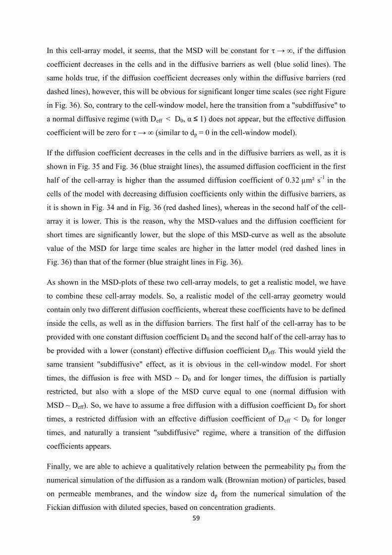
59

In this cell-array model, it seems, that the MSD will be constant for τ → ∞, if the diffusion

coefficient decreases in the cells and in the diffusive barriers as well (blue solid lines). The

same holds true, if the diffusion coefficient decreases only within the diffusive barriers (red

dashed lines), however, this will be obvious for significant longer time scales (see right Figure

in Fig. 36). So, contrary to the cell-window model, here the transition from a "subdiffusive" to

a normal diffusive regime (with Deff < D0, α ≤ 1) does not appear, but the effective diffusion

coefficient will be zero for τ → ∞ (similar to dp = 0 in the cell-window model).

If the diffusion coefficient decreases in the cells and in the diffusive barriers as well, as it is

shown in Fig. 35 and Fig. 36 (blue straight lines), the assumed diffusion coefficient in the first

half of the cell-array is higher than the assumed diffusion coefficient of 0.32 µm² s-1

in the

cells of the model with decreasing diffusion coefficients only within the diffusive barriers, as

it is shown in Fig. 34 and in Fig. 36 (red dashed lines), whereas in the second half of the cell-

array it is lower. This is the reason, why the MSD-values and the diffusion coefficient for

short times are significantly lower, but the slope of this MSD-curve as well as the absolute

value of the MSD for large time scales are higher in the latter model (red dashed lines in

Fig. 36) than that of the former (blue straight lines in Fig. 36).

As shown in the MSD-plots of these two cell-array models, to get a realistic model, we have

to combine these cell-array models. So, a realistic model of the cell-array geometry would

contain only two different diffusion coefficients, whereat these coefficients have to be defined

inside the cells, as well as in the diffusion barriers. The first half of the cell-array has to be

provided with one constant diffusion coefficient D0 and the second half of the cell-array has to

be provided with a lower (constant) effective diffusion coefficient Deff. This would yield the

same transient "subdiffusive" effect, as it is obvious in the cell-window model. For short

times, the diffusion is free with MSD ~ D0 and for longer times, the diffusion is partially

restricted, but also with a slope of the MSD curve equal to one (normal diffusion with

MSD ~ Deff). So, we have to assume a free diffusion with a diffusion coefficient D0 for short

times, a restricted diffusion with an effective diffusion coefficient of Deff < D0 for longer

times, and naturally a transient "subdiffusive" regime, where a transition of the diffusion

coefficients appears.

Finally, we are able to achieve a qualitatively relation between the permeability pM from the

numerical simulation of the diffusion as a random walk (Brownian motion) of particles, based

on permeable membranes, and the window size dp from the numerical simulation of the

Fickian diffusion with diluted species, based on concentration gradients.

60

Figure 37: Ratio of Deff and D0 for different values of pM (numerical simulation of the diffusion, based on permeable membranes with L = 500 nm and D0 = 0.32 µm²/s; blue dashed line), compared with the results of the numerical

simulation with different sized windows, based on concentration gradients (red straight line). The permeability is defined from 0 to 31.6 for Δτ = 1 ms and the window size is defined from 0 to L = 500 nm (left Figure: numerical simulation of Brownian diffusion; right Figure: numerical simulation of Fickian diffusion; both based on permeable membranes).

In Fig. 37, surprisingly, the agreement between the two diffusion models (based on permeable

membranes and based on concentration gradients) is obviously higher for the numerical

simulation of the Brownian diffusion (left Figure). However, we expected the agreement

between these two models being higher for the numerical simulation of the Fickian diffusion,

based on permeable membranes, as it is closer to the assumption of the cell-window model,

based on concentration gradients.

Nevertheless, we could show that there is a relation between the physically interpretable

window-, respectively pore-size of the cell-window model, which represents the mucus-pore

structure, and the permeability of the membranes in our abstracted numerical model.

The following Figures 38 and 39 show the resulting MSD from numerical simulations of the

Fickian and the Brownian diffusion, respectively, with different pM, equivalent to the results

from the cell-window model in Fig. 33. In addition, the differences in concentration -here,

concentration means the number of particles in relation to the total particle number- are

presented for the simulated Fickian and Brownian diffusion (right Figures). Hereby,

difference means the difference of the relative particle number in a distance to the permeable

membrane of 50 nm at the positive (+) and negative (-) position, equivalent to the results from

the cell-window model in Fig. 30.

61

Figure 38: Simulated MSD (left Figure) and the difference of concentration, respectively relative number of particles (right Figure), for Fickian diffusion of 200nm-sized particles with D0 = 0.32 µm²/s, L = 500 nm, and different

permeabilities. The time-dependent difference of the concentration (here, concentration means the relative number of particles, compared to their total number) has been calculated from the concentration at the left (-) and at the right (+)

side of the permeable membrane.

Figure 39: Simulated MSD (left Figure) and the difference of concentration, respectively relative number of particles (right Figure), for Brownian diffusion of 200nm-sized particles with D0 = 0.32 µm²/s, L = 500 nm, and different

permeabilities. The time-dependent difference of the concentration (here, concentration means the relative number of particles, compared to their total number) has been calculated from the concentration at the left (-) and at the right (+)

side of the permeable membrane.

Here, the transient anomalous ("subdiffusive") behavior becomes more obvious for the

Fickian diffusion, compared to the Brownian diffusion.

As already shown in Fig. 30, also here the difference of the concentration approximates to a

constant value for τ → ∞ and will be zero for pM = ∞ (equivalent to dp = L), in case of the

simulated Fickian diffusion. The simulation of the Brownian diffusion results in a difference

of zero for τ → ∞, independent on the permeability of the membrane, which only affects the

values at τ → 0.

62

4.4 Conclusions

We presented a model based on a cellular structure with permeable membranes [27] to

explain the experimental observed transient "subdiffusive" behavior of nanoparticles in

mucus. We applied this model to reproduce the MSD-curves from published particle tracking

experiments.

We showed that it is possible to predict the particle diffusivity in mucus for short and long

time limits by an in-silico model, based on permeable membranes. Therefore, we have to

assume only three parameters, which are the distance of the membranes L, the diffusion

coefficient for short time limits D0, and the permeability of the membranes pM, resulting in a

diffusion coefficient for long time limits Deff. We are able to replace particle-tracking

experiments by numerical simulations, if we know the properties of the particles and the

investigated mucus. Different particle coatings and particle sizes, as well as the mucus

properties lead to specific permeabilities pM, and the mucus pore-, respectively mesh-size is

related to the mean cavity size L. Naturally, the particle size and the permeability affects the

diffusion coefficient for short D0 and long Deff time limits, respectively.

Additionally, we showed different mean passage times and percentages of particles, passing

the mucus layer for various assumptions of L and pM, as well as for certain particle and mucus

properties. The advantage in using our model is obviously, that we are able to calculate the

MSD and to determine the corresponding pdf for the short and long time limits, which is

currently not possible with experimental methods. In experiments, the MSD only in a short

time range is measureable and the measurement of the pdf is still a current topic. However, by

the usage of our model, one can compute the MSD and the pdf, both in large time ranges and

just by assuming only three essential parameters. These parameters contain all physical and

chemical properties of mucus and of the particles.

Due to its confined geometry, mucus is shown to be an excellent heterogeneous material

model to predict the transient "subdiffusive" regime within the experimentally measurable

time range. The model includes two physically interpretable diffusion coefficients D0(η;R) for

shorter times and Deff(pM) for longer times, as well as the distance L between the membranes.

The assumed viscosity of the interstitial fluid is similar to that of water. The permeability of

the membranes is characterized by pM, affecting Deff. We discussed a heuristic analytic

approximation formula for the MSD(τ) with the parameters D0, Deff, and L. The

approximation was substantiated by detailed numerical simulations based on permeable

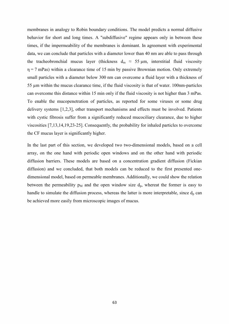
63

membranes in analogy to Robin boundary conditions. The model predicts a normal diffusive

behavior for short and long times. A "subdiffusive" regime appears only in between these

times, if the impermeability of the membranes is dominant. In agreement with experimental

data, we can conclude that particles with a diameter lower than 40 nm are able to pass through

the tracheobronchial mucus layer (thickness dm ≈ 55 µm, interstitial fluid viscosity

η = 7 mPas) within a clearance time of 15 min by passive Brownian motion. Only extremely

small particles with a diameter below 300 nm can overcome a fluid layer with a thickness of

55 µm within the mucus clearance time, if the fluid viscosity is that of water. 100nm-particles

can overcome this distance within 15 min only if the fluid viscosity is not higher than 3 mPas.

To enable the mucopenetration of particles, as reported for some viruses or some drug

delivery systems [1,2,3], other transport mechanisms and effects must be involved. Patients

with cystic fibrosis suffer from a significantly reduced mucociliary clearance, due to higher

viscosities [7,13,14,19,23-25]. Consequently, the probability for inhaled particles to overcome

the CF mucus layer is significantly higher.

In the last part of this section, we developed two two-dimensional models, based on a cell

array, on the one hand with periodic open windows and on the other hand with periodic

diffusion barriers. These models are based on a concentration gradient diffusion (Fickian

diffusion) and we concluded, that both models can be reduced to the first presented one-

dimensional model, based on permeable membranes. Additionally, we could show the relation

between the permeability pM and the open window size dp, whereat the former is easy to

handle to simulate the diffusion process, whereas the latter is more interpretable, since dp can

be achieved more easily from microscopic images of mucus.

64

5 Mechanical and Rheological Properties of Mucus

5.1 Introduction

5.1.1 Macro- and microrheology of mucus

Mucus is a biological hydrogel with a highly inhomogeneous and complex structure with

unique viscoelastic properties [3,9,65-68]. As a consequence mucus represents also an

important biological barrier that prevents immediate access to the surface of mucosal

epithelial cells which holds for both molecules as well as particles. Macrorheological

properties, which are expressed by the elastic storage and the viscous loss modules, G` and

G`` respectively, can be determined for the entire mucus structure as a consequence of a

reshape and reorientation of the mucin fibers. Both parameters are generally determined by

frequency- and amplitude-sweeps in a rheometer. Microrheological properties are expressed

by the viscosity of the interstitial fluid and the elasticity of single mucin fibers. Latter can be

determined by active measurements, using optical tweezer, whereas the viscosity of the

interstitial fluid is determined by passive Brownian motion. In rarely cases, also a meso-phase

rheology is described by the retarded movement of Brownian particles due to steric

hindrances [3]. This restricted movement of particles by topological properties of the mucus

mesh has been investigated in the first part of this work.

5.1.2 Viscoelastic properties of mucus

In the same way as mucus function may differ from organ to organ (e.g., lubrification,

protection, etc.), its viscoelastic properties are also likely to be different according to the

respective biological needs. In order to address this hypothesis, we have chosen to compare

mucus from the intestinal and the respiratory tract as mucus from either organ has to perform

rather different functions. The pig was chosen as mucus from this source can be obtained

relatively easily, also considering ethical aspects. To compare the viscoelastic properties, the

elastic storage as well as the viscous loss modules will be measured by different methods,

regarding micro- and macroscopic length scales. The elastic storage module G` describes the

elastic part -similar to a spring constant- of the mucin fibers, whereas the viscous loss module

G`` describes the viscous, dampening part of the fluid.

65

In the first part of this thesis, we assumed the fluid to be purely viscous, which is expressed

by a constant fluid viscosity, independent on the shear rate (see Fig.1 in [3]), and we also

assumed the permeable membranes to be rigid. These assumptions were made to simulate the

Brownian motion of freely diffusing particles inside the mucus mesh (microscopic rheology).

To simulate the mechanical behavior of the mucin fibers, respectively the entire mucus

structure (macroscopic rheology), we assume the fibers to be linear elastic, which is expressed

by constant Young`s modules, linear dependent on the shear rate (see Fig.1 in [3]). These

assumptions are in good agreement with the real viscoelastic properties of mucus, where the

mucin fibers are known to be semiflexible, and the interstitial fluid is known to be purely

viscous with a viscosity, similar to that of water, typically in the order of few mPas. However,

the entire mucus structure has viscoelastic properties.

The following Table 4 shows different values for the G` and G``, as well as different

macrorheological viscosities of mucus from various species and organs.

Table 4: Exemplary rheological studies of mucus from different species and organs.

Ref. Species Organ Macro η [Pas] G` [Pa] G`` [Pa]

[11] Human Lung 10 at 1 rad/s 10 at 1 rad/s 4 at 1 rad/s

[14] Human Lung (CF) 70 at 0.1 s-1

- -

[18] Human Cervical 1 at 1 s-1

- -

[13] Human Lung (CF) - 95 at 1 rad/s 22 at 1 rad/s

[13] Human Lung

(COPD)

- 3 at 1 rad/s 1 at 1 rad/s

[3] Human Cervical 40 at 1 rad/s - -

[3] Human Lung 5 at 1 rad/s - -

[3] Human Lung

(Bronchitis)

10 at 1 rad/s - -

[3] Human Lung (CF) 20 at 1 rad/s 7 at 1 rad/s 3 at 1 rad/s

[3] Dog Subglottis 1-20 at 1 rad/s 5-63 at 1 rad/s 1-20 at 1 rad/s

[3] Pig Intestinal 0.1-5 at 1 rad/s 0.2-10 at 1 rad/s 0.1-6 at 1 rad/s

[3] Rat Trachea 0.01-3 at 10 rad/s 2-8 at 10 rad/s 0.2-6 at 10 rad/s

[3] Horse Trachea 0.6-1 at 10 rad/s 18-34 at 10 rad/s 6-12 at 10 rad/s

[3] Rabbit Trachea 35-130 at 1 rad/s - -

[3] Ferret Trachea 12-110 at 1 rad/s - -

[69] Pig Trachea - 3 at 1 s-1

2 at 1 s-1

[70] Pig Gastric 10-100 at 1 rad/s 20-200 at 1 rad/s 3-30 at 1 rad/s

The rheological properties, in particular the macrorheological parameters G` and G``, are

important to calculate the deformation of the mucin fibers due to the particle impact.

Therefore, we need to simulate the fluid dynamics in the lung and compute the resulting

kinetic energy of inhaled particles. After comparing this energy with the necessary

deformation energy to expand the mucus pores -after a deformation of the mucin fibers- we

will qualitatively determine the possibility of a particle to penetrate one mucus pore.

66

5.2 Macro- and microrheological properties of native porcine respiratory and

intestinal mucus

Parts of this chapter have been published in Bokkasam H., M. Ernst, M. Günther, C. Wagner,

U. F. Schäfer, and C.-M. Lehr (2016). Different macro- and micro-rheological properties of

native porcine respiratory and intestinal mucus. International Journal of Pharmaceutics

510(1):1-12.

5.2.1 Materials & Methods

Mucus was collected from pigs used for experimental surgery studies, which had to be killed

afterwards. Therefore, no animals had to suffer or to be sacrificed to obtain this biological

material, in line with the 3R-concept. Care was taken that the preceding surgery experiments

had no influence on the organs relevant to our studies. Mucus was collected within 30 minutes

after euthanasia. The trachea was cut into halves [68] and mucus was obtained by carefully

scratching. Intestinal mucus was harvested from the ileum and duodenum of the same animal

after a short rinse with water [67].

For comparison, HEC gels of 1 and 2 % (w/v) were prepared using NatrosolHHX 250

(Hercules Aqualon, Düsseldorf, Germany).

Macrorheological studies of storage and loss module (G` and G``) were performed with a

25 mm plate-plate geometry in a MARS II rheometer (ThermoHaake, Karlsruhe, Germany) as

used in previous studies [66,67]. The volume of the mucus samples, put in the rheometer, was

between 20 and 30 µL, resulting in a gap distance between 40 and 60 µm. Measurements at

1 Hz were used for comparison.

Passive and active microbead rheology with optical tweezers provides a promising laser-based

method for investigating the Brownian motion and induced movement of microparticles in a

laser trap [8,71]. A Tweez250i system from Aresis (Ljubljana, Slovenia) was utilized.

Melamine resin beads of 2.86 and 6 µm diameter were purchased from Microparticles GmbH

(Berlin, Germany). Sample preparation was performed for both mucus and HEC gels as

described in previous experimental studies [8].

Passive microbead rheology was studied by recording the restricted Brownian motion of

microparticles at a frame rate of approx. 670 fps. Based on the experimental conditions,

67

mainly the viscosity of the interstitial fluid in the mucus pores is measured by this method.

For more details see supplementary material.

Active microbead rheology was performed by applying a sine wave (Frequency = 0.1 Hz and

Amplitude = 1 µm) to microparticles. The amplitude of particle movement (output

displacement response) to an input displacement of 1 µm is measured from the displacement

of the particle over time. As the amplitude of this active particle movement is at least 10times

larger than the movement in passive microbead rheology measurements, additional

macrorheological effects cannot be excluded.

OriginPro 2015 (Northampton, USA) and One-way ANOVA were used for Box-and-whisker

plots as well as for statistical calculations. Moreover the Scheffé`s method as post hoc

analysis was applied. The level of statistical significance is indicated by the corresponding p-

value.


Viscoelastic properties of porcine mucus from ileum, duodenum and trachea are depicted in

Fig. 41. One-way ANOVA reveals statistically significant (p < 0.05) differences between

intestinal and respiratory mucus, but there is no significant difference between mucus from

ileum and duodenum. In Figure 40 the frequency sweep of the rheometric measurements from

Figure 41 is shown. We used a frequency of 1 Hz (6.3 rad/s) to compare the results from the

rheometry with them of the active and passive microbead rheology measurements with optical

tweezer. However, the macrorheological elastic (red solid lines) and viscous (blue dashed

lines) modulus strongly depends on the frequency of the rheometer.

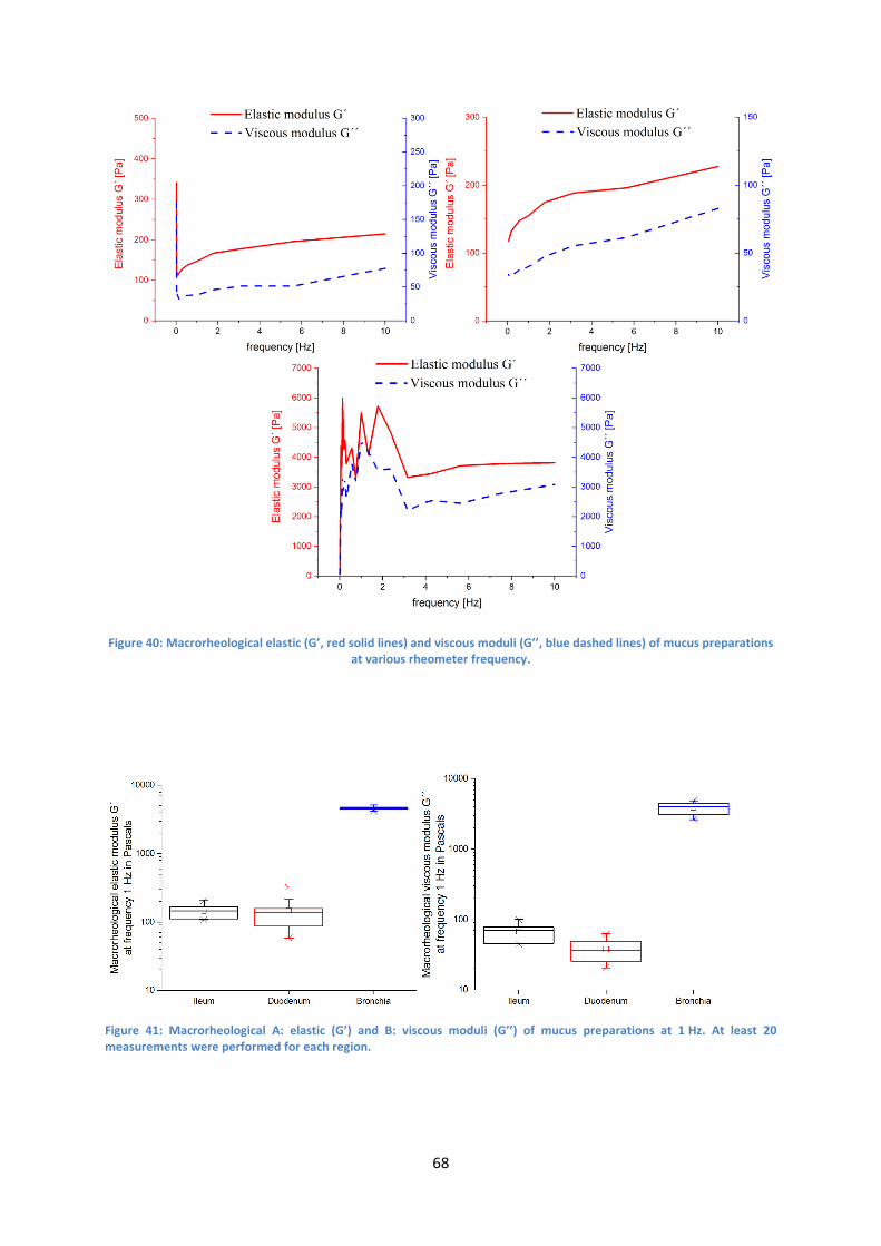
68

Figure 40: Macrorheological elastic (G’, red solid lines) and viscous moduli (G’’, blue dashed lines) of mucus preparations at various rheometer frequency.

Figure 41: Macrorheological A: elastic (G’) and B: viscous moduli (G’’) of mucus preparations at 1 Hz. At least 20 measurements were performed for each region.

69

Fig. 42 shows the results of the elastic storage modulus G` measurements from passive

microbead rheological studies by means of optical tweezers for 2.86 and 6 µm particles (for

more details see supplementary material). In contrast to the macrorheological investigations,

no statistically significant (p > 0.05) differences are found between intestinal and respiratory

mucus for both 2.86 and 6 µm beads. It can be concluded that there are no microrheological

differences between intestinal and respiratory mucus obtained from the same mammalian

species (pig).

Figure 42: Microrheological elastic moduli (G’) with optical tweezers for (A) 2.86 µm and (B) 6 µm beads. At least 20 measurements were performed for each region.

Fig. 43 reveals that microparticle movement in HEC gels (A, B; red dashed line) has similar

pattern to particle movement in water (black straight line) but not in either respiratory or

intestinal (ileal) mucus (C, D; red dashed line). Here, 6 µm particle movement is shown as an

instance of the motion of (micro)particles in complex structures and the same holds true for

2.86 µm particles. These findings correlate with previous studies on equine respiratory tract

mucus preparations with optical tweezers [8].

70

Figure 43: Optical trap displacement in µm of a 6 µm particle in (A) HEC-1%, (B) HEC-2%, (C) respiratory, and (D) ileal mucus (red dashed lines). Displacement of particles in water is shown as a black solid line in each graph for comparison. At least 20 measurements were performed for each region.

Active microbead rheology (output displacement response) measures the force of the beads

against single mucin fibers and the resistance to the bead movement. One-Way ANOVA

reveals statistically significant differences (p < 0.05) between such data for pulmonary and

intestinal mucus, whereas no statistically significant differences were found between ileal and

duodenal mucus (Fig. 44). The higher output displacement response for 2.86 and 6 µm beads,

as observed for pulmonary mucus in comparison to intestinal mucus, can be explained by

either a lower rigidity of pulmonary mucin fibers or a larger mesh size for the pulmonary

mucus network. This finding points to differences in the mucus barrier function between the

investigated organs, i.e. intestine and lung, and route of administration.

71

Figure 44: Output displacement response in µm of mucus preparations for (A) 2.86 µm and (B) 6 µm beads. At least 20 measurements were performed for each region.

In Table 5 the measured G` and G`` from our experiments (*) are compared with the

corresponding data from other studies, as shown in Table 4. Only the best fitting data from

these studies are presented in comparison with our results.

Table 5: Comparison of the experimentally determined rheology parameters (see columns marked with asterisks, red labeled results from passive microbead rheology methods) with the results from previous studies (see Table 4).

Ref. Species Organ Macro η

[Pas]

G` [Pa] G`` [Pa] G` [Pa] *

[11] Human Lung 10 at 1

rad/s

10 at 1 rad/s 4 at 1

rad/s

12

[13] Human Lung (CF) - 95 at 1 rad/s 22 at 1

rad/s 80

[3] Dog Subglottis 1-20 at 1

rad/s

5-63 at 1 rad/s 1-20 at 1

rad/s

12 / 24 / 30

/ 46 / 50 /

60

[3] Pig Intestinal 0.1-5 at 1

rad/s

0.2-10 at 1

rad/s

0.1-6 at 1

rad/s

12

[3] Horse Trachea 0.6-1 at

10 rad/s

18-34 at 10

rad/s

6-12 at

10 rad/s

12 / 24 / 30

[70] Pig Gastric 10-100 at

1 rad/s

20-200 at 1

rad/s

3-30 at 1

rad/s

24 / 30 / 46

/ 50 / 60 /

80 / 150

Here, the red labeled values are measured by passive microbead rheology methods (see

Fig. 42), whereas the remaining values are from conventional plate rheometry measurements

(see Fig. 41). Surprisingly, the measured G` and G`` of bronchial mucus in the rheometer are

extremely high (several thousand Pascal), which may be due to a progressed drying of our

72

mucus samples or maybe the scratching out of the mucus from the lung epithelial was not

carefully enough to avoid some residues of the epithelial in the samples. However, except

these extremely high G-values from experiments with bronchial mucus, the measured G`-

values from the experiments, which are shown in Fig. 41 (rheometry: G` = 150 Pa) and

Fig. 42 (optical tweezer: G` = 12-80 Pa), are comparable to the results from other studies.

Only the G``-values are significantly higher (40-70 Pa) in our experiments, compared to the

results from other studies in Table 4.

73

5.3 Calculation of the necessary deformation energy to expand the mucus pores

5.3.1 Computation of the deflection and deformation of mucin fibers

To investigate the possibility for inhaled particles to penetrate the mucus layer, the elastic

deformation of mucin fibers will be calculated in this section. We assume linear elastic fibers

to calculate this deformation by numerically computing the necessary energy to achieve a

prescribed deflection, respectively pore expansion, solving the bending equation.

The aim of these calculations is to compute the expansion of the mucus pore, which is

modeled as the void between two fibers. Due to the deflection of the fiber, e.g. in the y-

direction, there is also a deformation in the x-direction. This effect leads to a symmetrically

expansion of the mucus pore, if we assume a particle impact exactly in the center of the pore

and also a consistent fiber length, in case of a deflection vertically to the fiber position (see

Fig. 45). Finally, we qualitatively determine the possibility of a 200nm-sized particle to move

through a 100nm-sized pore.

The order to determine the probability of a particle to pass the mucus pore is first: to compute

the needed energy to expand the mucus pore in a way, that allows the particle to completely

pass the pore; and: to compare the kinetic energy from the CFD-simulations in the next

section with this deformation energy. Additionally, we will also compare the necessary

deformation energy with the Brownian kinetic energy of the same particle.

In this section, we first calculate the deflection f of the mucin fibers by solving the general

deflection equation, given as follows [72]:

lsxMIE

fM

1

(23)

with the Young`s modulus E, the second moment of area IM (the product E∙IM is the bending

stiffness), the sum of all force moments ΣM(x), the curved section s, and Δl as the distance

between the center of s (during deflection) and the end of the mucin fiber.

The second moment of area IM is defined as follows [72]:

74

12

123

3

hbyI

andhb

xI

M

M

(24)

with the width b and the height h of the mucin fiber. To simplify, we assume the fibers to be

as wide as high (h = b).

Due to the difficulties in determining the curved section s of a deformed object and therefore

in calculating the deflection analytically, consequently, we will compute the deflection

numerically, using the Finite Element Method.

As we assume a linear elastic material, the Hook´s law is valid to calculate the elastic strain

εel, as given by:

E

elel

(25)

with the assumed elastic stress σel. The elastic strain is then computed in the structural

mechanics module of Comsol Multiphysics by using the deformation w and numerically

solving the following equation:

ww

with

T

inelel

2

1

(26)

with the inelastic part of the strain εinel and the total strain ε.

Here, a mesh with homogeneous triangular elements with a size between minimum 0.1 and

maximum 1 nm is implemented to discretize the fiber geometry. To solve the differential

equations, a parallel sparse direct stationary solver is used.

75

For the sake of completeness, we also show, how to calculate the deflection by using the

theorem of Pythagoras and the analytical solution of the deflection f, assuming the fibers to be

linear elastic, as given as follows [72]:

.3

13

2

;16

2

0

0

2

0

2

0

endsbothatfixedisfibertheiflx

endoneatonlyfixedisfibertheiflx

withendsbothatfixedisfibertheifIE

lFxf

endoneatonlyfixedisfibertheifIE

lFxf

M

M

(27)

with the assumed impact force F of the particle and the length of the fiber l.

The expansion of the mucus pore is calculated by using the deflection of the mucin fiber f and

the length l of the fiber, which is assumed to stay constant in case of a deflection vertically to

the fiber position (see Fig. 45). Thus, the expansion of the pore pexp is given as:

22

exp fllp (28)

Fig. 45 shows the geometrical model of the mucus pore as a gap between two mucin fibers,

which are modeled as two thin beams in this work. Additionally, this Figure summarizes the

mentioned assumptions to calculate the expansion of the mucus pore (deformation in blue), as

well as the extension of the mucin fiber (deflection in red). It also shows the assumed

boundary conditions of the numerical model.

76

Figure 45: Schematic view of two mucin fibers and one void between these fibers, which is defined to be the mucus pore (upper Figure). The mucus pore has to be expanded to achieve a penetration of a larger particle. Schematic view of the mechanical deformation, leading to an expansion of the mucus pore (blue dash-dotted lines) due to the deflection of the mucin fiber (red dashed lines), and the angle of inclination between the initial fiber position and the position after mechanical load.

As mentioned, after the deflection of the fibers, the size of the void, respectively the mucus

pore dp, should increase to let the particle pass through.

So, we presented two ways to calculate the deflection of a mucin fiber, which are the

numerical simulation with the deflection w and the analytical solution with the resulting

deflection f. Both values can be achieved by two different methods: We could assume an

impact force F of an inhaled particle or we could prescribe the deflection to yield a necessary

pore expansion for the particle to pass through. The former method is an iterative process,

where we have to find the minimum kinetic energy of a particle to achieve the necessary force

F to deform the fiber, resulting in a pore expansion. In the latter method we prescribe the pore

expansion to be pexp = 2R - dp, with the hydrodynamic radius R of the particle. We then

compute the necessary deformation energy to achieve the prescribed pore expansion.

We assume a necessary expansion of the pore pexp = 100 nm (R = 100 nm, dp = 100 nm), a

Young´s modulus of 100 Pa, and a mucin fiber density of 1000 kg/m³.

deflection = extension of the fiber in y-direction

deformation = expansion of the pore in x-direction

angle of inclination

prescribed deflection in

the y-direction

prescribed deformation in

the x-direction

no displacement at

the left boundary

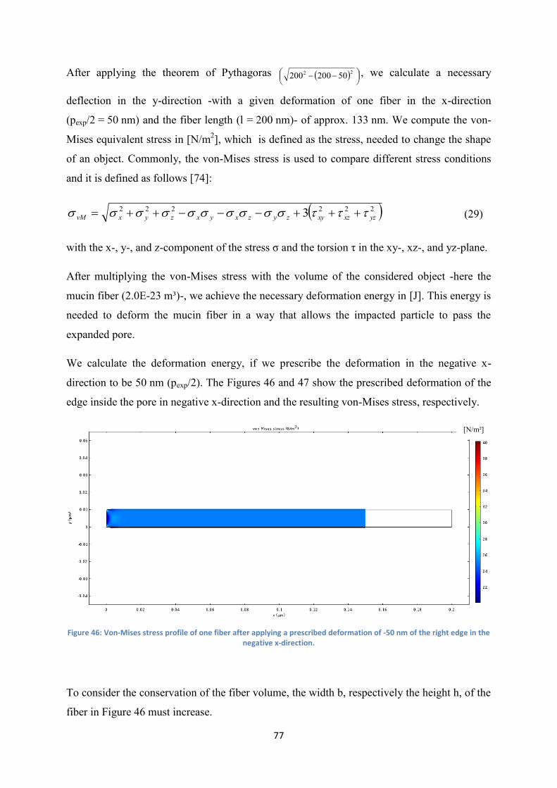
77

After applying the theorem of Pythagoras

22 50200200 , we calculate a necessary

deflection in the y-direction -with a given deformation of one fiber in the x-direction

(pexp/2 = 50 nm) and the fiber length (l = 200 nm)- of approx. 133 nm. We compute the von-

Mises equivalent stress in [N/m2], which is defined as the stress, needed to change the shape

of an object. Commonly, the von-Mises stress is used to compare different stress conditions

and it is defined as follows [74]:

222222 3 yzxzxyzyzxyxzyxvM (29)

with the x-, y-, and z-component of the stress σ and the torsion τ in the xy-, xz-, and yz-plane.

After multiplying the von-Mises stress with the volume of the considered object -here the

mucin fiber (2.0E-23 m³)-, we achieve the necessary deformation energy in [J]. This energy is

needed to deform the mucin fiber in a way that allows the impacted particle to pass the

expanded pore.

We calculate the deformation energy, if we prescribe the deformation in the negative x-

direction to be 50 nm (pexp/2). The Figures 46 and 47 show the prescribed deformation of the

edge inside the pore in negative x-direction and the resulting von-Mises stress, respectively.

Figure 46: Von-Mises stress profile of one fiber after applying a prescribed deformation of -50 nm of the right edge in the negative x-direction.

To consider the conservation of the fiber volume, the width b, respectively the height h, of the

fiber in Figure 46 must increase.

[N/m²]

78

In Fig. 47, the von-Mises stress is shown at the intersection of the fiber at y = 0.005 µm.

Figure 47: Von-Mises stress at the intersection at y = 0.005 µm in x-direction of one fiber after applying a prescribed deformation of -50 nm of the right edge in the negative x-direction.

In the Figures 48 and 49 the displacement of the middle point of the edge inside the pore is

prescribed in the negative y-direction (133 nm), and the resulting von-Mises stress is shown.

Figure 48: Von-Mises stress profile of one fiber after applying a prescribed deflection of approx. -133 nm of the middle point (y = 0.005 µm) of the right edge in the negative y-direction.

To consider the conservation of the fiber volume, the width b, respectively the height h, of the

fiber in Figure 48 must decrease. However, the deformation in Fig. 48 is not shown in a

proper way, due to the assumption of a constant geometric ratio between the width b, the

height h, and the length l of the fiber (see Fig. 45).

[N/m²]

79

In Fig. 49, again the von-Mises stress is shown at the intersection of the fiber at y = 0.005 µm.

Figure 49: Von-Mises stress at the intersection at y = 0.005 µm in x-direction of one fiber after applying a prescribed deflection of approx. -133 nm of the middle point (y = 0.005 µm) of the right edge in the negative y-direction.

All computed values are determined in Joule per cubic meters (N/m² = J/m³), which means the

energy in Joule, needed to deform an object with a volume of 1 m³. Consequently, to

determine the necessary deformation energy of the fiber, we have to multiply the von-Mises

stress by the volume of the fiber (2.0E-23 m³). This calculation results in a deformation

energy of 2.2E-24 J in case of a prescribed deflection in the y-direction (see Figures 48 and

49), and of 5.0E-22 J in case of a prescribed deformation in the x-direction (see Figures 46

and 47). As expected, the necessary deformation energy is lower in case of a vertically

deflection of the mucin fibers, e.g. by an impaction of an inhaled particle.

In addition, we have to consider the fact that, in case of a doubling of the length of the fiber,

the moment M at the edge of the fiber will double, too. However, if the width or the height of

the fiber is doubled, the second moment of area IM will be 8fold higher than before,

respectively in case of h = b, IM will be 16fold higher. So, if other geometries and length

scales of the fiber will be investigated in future, one has to consider this fact, which will yield

in totally different -probably higher- necessary deformation energies.

80

5.3.2 Brownian diffusive energy and comparison with the necessary deformation energy

The necessary deformation energy, which is computed by the numerical simulations of the

deflection of a mucin fiber will be compared with the kinetic energy from convective flow of

an aerosol (see Table 9 and Table 10) and also with the kinetic energy of Brownian motion,

whereat the latter is given by:

TkE BBrown2

3 (30)

Thus, we will check the possibility of a particle to penetrate a mucus pore by either impaction

due to the air flow (kinetic energy from CFD-simulations) or by Brownian motion. For a

given Boltzmann constant of 1.38E-23 J/K and an assumed absolute temperature of 310.15 K,

we yield a Brownian kinetic energy of 6.24E-21 J. So, this energy would be sufficiently high

enough to achieve a pore expansion, allowing the particle to pass through this pore, just by

Brownian diffusion (with the assumed fiber dimensions and parameters, as described in the

prior section).

The Brownian kinetic energy as shown in Eq. 30 contains only the Einstein-component -the

thermal energy- of the Stokes-Einstein-relation. If we consider also the Stokes friction force,

which is present in case of particle diffusion, the kinetic energy of the Brownian motion will

be reduced. As shown in Eq. 12, the Stokes friction force depends on the viscosity of the

fluid, the particle size, and the relative velocity of the particle in a flowing fluid. However, the

Brownian kinetic energy is higher for smaller particles and in fluids with a lower viscosity.

So, as we assume the fluid viscosity to be similar to that of water, extremely small particles in

the nm-range yield in a significantly higher Brownian diffusive energy, compared to

microparticles. Due to the fact that, the thermal energy of a Brownian particle is at least

10fold higher than the calculated necessary deformation energy, the effects of the Stokes

friction force on the Brownian kinetic energy is vanishing.

81

5.4 Conclusions

Macrorheological investigations (plate–plate viscosimetry) on mucus obtained from the

respiratory (trachea) and intestinal tract (ileum and duodenum) of the same species (pig)

revealed significant differences in viscoelastic properties for these two organs. Passive

microbead rheological measurements (particle tracking of Brownian dynamics), taking place

only in the interstitial fluid of the mucus pores, are not able to detect these differences.

However, active microbead rheology measurements (induced movement by optical tweezers)

again revealed significant differences between respiratory and intestinal mucus, pointing to

biomechanical differences in the constituting mucin fibers or structural differences in the

resulting hydrogel networks.

We computed the necessary deformation energy of a mucin fiber to achieve a penetration of a

particle through an expanded mucus pore. The possibility of such a particle to pass this pore

will be qualitatively described in the following section in case of a convective air flow.

However, we showed that the Brownian diffusive energy of a particle should be high enough

to achieve a vertical deflection of the mucin fiber and even high enough to achieve a

horizontal deformation of the fiber, both resulting in an expansion of the pore. The latter case

was shown to need a significantly higher energy to yield the required pore expansion,

allowing the particle to pass the pore.

82

6 Computational Fluid Dynamics (CFD) Simulations of the Air Flow in

the Human Lung

6.1 Introduction

6.1.1 Structure of the human lung

The human lungs are responsible for the gas exchange between the atmospheric air and the

blood. The right lung, pulmo dexter, is larger and consists of three lobes, the superior, the

middle and the inferior lobe. The left lung, pulmo sinister, consists only of a superior and an

inferior lobe, leaving space for the heart in the chest cavity. Breathing air passes the trachea

and flows into the lobes that contain a large system of air-carrying tubes, the respiratory

tree [75].

However, in this work only the trachea and the upper part of the respiratory tree, the main

bronchi, are considered. The left and right main bronchus, bronchus principalis sinister and

bronchus principalis dexter, respectively, are branching of from the trachea. The right

bronchus is wider in radius, shorter until it branches out and steeper in the angle, which leads

to an asymmetry of the lungs and to a higher accumulation of foreign substances in the right

bronchus. The left bronchus is less steep than the right bronchus, again to leave space for the

heart cavity. The angle γB between the two main bronchi is between 55 and 70° [75,76].

Fig. 50 shows a schematic view of the human lung [77].

Figure 50: Structure of the human lung with the oral and nasal cavity (blue region), the upper respiratory tract (green region), and the lower respiratory tract (red region), Oberdörster et al. [77].

83

6.1.2 Development of lung models

Aim of the simulation of the air flow in the upper lung is to determine the velocity profile in

different regions of the upper airways and to compute the kinetic energy of inhaled particles,

impacting on the mucus layer in these regions.

Air is used as continuous fluid to simulate the flow dynamics in the upper airways, modeled

as a simplified symmetrically geometry and as a more realistic non-symmetrically geometry

(see Fig. 51 and Fig. 52, respectively). In both Figures, on the right side, the velocity profile is

shown for an inlet velocity of 1 m/s.

Figure 51: Simplified symmetrical model of the human lung with the velocity profile on the right side (inlet velocity is 1 m/s).

Figure 52: Simplified asymmetrical model of the human lung with the velocity profile on the right side (inlet velocity is 1 m/s).

84

For the CFD-simulations, in a first geometrical model, the larynx and the trachea are

interpreted as a pipe with a diameter of 1.5 cm and with a 90°-turn after 9 cm. After additional

21 cm, the main bronchi, which are also modeled as pipes with a diameter of each 1.5 cm, are

branching of in a 90°-turn, followed by a second 90°-turn (see Fig. 51). To improve this

model of the upper airways, we also introduce a more realistic non-symmetrically model (see

Fig. 52) with a steeper angle for the right bronchi, compared to the left bronchi, resulting in an

asymmetry.

To improve our model, we also introduce a further geometrical lung model, which directly

considers the mucus layer, as steric hindrances within the trachea (see Fig. 53).

Figure 53: Realistic model of the human trachea with steric hindrances, representing the mucus layer, with the velocity profile on the right side (inlet velocity is 1 m/s).

In general, flow rates between 5 and 15 l min-1

are assumed to simulate the inhalation of an

aerosol, which leads to inlet velocities between 0.5 and 1 m s-1

, assuming a tube diameter of

1.5 cm. In the FEM-model, a no-slip boundary condition is used, which means that the fluid

velocity u is zero at the boundary.

There exist two essential parameters for the flow of aerosols and particulate matter in a fluid,

which are the Reynolds and the Stokes number. The former describes the fluid flow regime,

whereas the latter describes the drag and the inertia of a particle, which is transported within a

fluid by a convective flow. The Stokes number is defined as [75,78,79]:

Lf

p

D

uRSt

18

22

(31)

85

with the particle density ρp, the fluid velocity u, the characteristic length, respectively the

characteristic dimension, DL, and the kinematic viscosity µf of the fluid.

The typical mean ventilation rate for a sitting and awake adult man is 150 mL s-1

[75], which

results in a flow velocity of 0.85 m s-1

, assuming an inner diameter of DL = 1.5 cm, as referred

to our lung model. This leads to a Reynolds number of 750, assuming a fluid density of

1.0 kg m-3

and a dynamic viscosity of the air of 17 µPas. The Reynolds number describes the

regime of a fluid flow (turbulent or laminar flow) and is calculated as given by [75]:

f

LLf DuDu

Re (32)

with the fluid density ρf, the kinematic viscosity µf, and the dynamic viscosity η.

Due to the low Reynolds number of 750, we assume a laminar flow of the air in the upper

lung. The essential equation to simulate an incompressible laminar flow is the Navier-Stokes-

equation, given as follows [23]:

ext

T

flf FuuIpuu (33)

with the pressure pl inside the lung. Here, no external force Fext are considered.

The discretization of the geometry is done with homogeneous triangular mesh elements with a

size between minimum 0.1 and maximum 2 cm and additional homogeneous rectangular

mesh elements at the boundary to achieve a high accuracy of the numerical solution in the

boundary layer. To solve the differential equation system, a parallel sparse direct stationary

solver for the laminar flow is used.

During the inhalation, an absolute pressure of 0.4 kPa at the outlet of the main bronchi is

assumed [80]. Due to an increase of the lung volume during the inspiration, the pressure is

reduced to a slight vacuum, compared to the atmospheric pressure outside of the lung. So, in

our model of the respiratory tract, we define the inlet velocity as shown in Table 8, and the

outlet pressure to be 0.4 kPa.

As we assume an overdamped movement of the particles in the air stream, external forces,

such as the drag force or the gravity are neglected, so the Stokes-number is no longer needed.

86

However, in our study we assume the particle velocity v to be identically with the fluid

velocity u and to be stationary, which means v is constant over the time. Consequently, we

can calculate the kinetic energy of the particles as given by:

2

2

1vmE pkin (34)

with v and mp as the particle velocity and mass, respectively. To calculate the kinetic energy

of the inhaled particles, we just need the simulated fluid velocity u (= v) and the particle mass

mp. We show simulated values of the kinetic energy in Table 8 and we compare them with the

necessary deformation energy and the Brownian diffusive energy in the Tables 9 and 10.

As mentioned before in Eq. 30 (definition of the Brownian diffusive energy), also here we did

neglect the Stokes friction force, due to the assumption of an overdamped movement.

Additionally, if we assume a convective flow of microparticles in air and a Brownian motion

of nanosized particles (nanoparticles are released from microparticles) in a fluid with a

viscosity similar to that of water, the Stokes friction force is equally for both cases and can be

neglected.

6.1.3 Particle deposition processes

There are four main processes, which are relevant to the deposition of particulate matter in the

lung: the impaction due to the convective air flow -which will be simulated in the next

paragraph-, the sedimentation, the interception, and finally the Brownian motion.

In the upper airways, the diameter of deposed particles differs in each region. In the larynx

mostly extremely small particles in the range of few nm and extremely large particles with a

diameter of about 1-10 µm can be found. In the tracheobronchial region, the typically particle

size is between 1 and 100 nm, but also very large particles in a range of a few µm can depose

in this region [77,81]. In the field of drug delivery, it is common to use particulate matter with

a size of several µm as an aerosol, being inhaled in the upper lung. These particle will depose

in the upper trachea by a convective flow and then release significantly smaller particles,

which are able to penetrate the mucus layer by diffusion.

87

Due to the low Reynolds number, we assume a laminar flow in the lung. Additionally, we can

also neglect the sedimentation effect of particles, due to their negligible mass. Nevertheless,

the particle mass will be considered to calculate the kinetic energy, as shown in Eq. 34, but to

simplify, in this study we use impaction as the only essential deposition effect to simulate the

particle deposition in the lung. In our model, Brownian motion, which mostly appears in the

alveoli, and interception, which is similar to a filtration effect and mainly appears for

filamentous particles, also do not play a role for simulating the particle deposition in the upper

airways.

There exist studies, which deal with the simulation of the air flow and the particle deposition

in the lung. To compare our results, the following Table 6 shows the average velocity in

different regions of the human lung and also the size of the particles, which are mostly found

in these regions. These values are from different published studies, dealing with the

simulation of particle deposition in the lung due to a convective air flow. The inlet velocity,

respectively the percentage of deposed particles are shown in brackets.

Table 6: Exemplary studies of CFD in the human lung to simulate the velocity and size distribution of particles in different regions of the lung (the inlet velocity, respectively the percentage of the deposed particles are shown in brackets).

Ref. Velocity [m/s] in bronchia Particle size [µm]

in larynx

Particle size [µm]

in trachea

Particle size [µm]

in bronchia

[79] 0.7-0.8 (1.2) - 10 (35) 8-10 (10-7)

[82] - 0.001 (6) 0.001 (10) 0.001 (3)

[83] - - 0.001 (33) 0.001 (29)

[78] - 0.001 (36) 0.001 (15-36) 0.001 (15)

[84] 0.1 (2.0) - - -

6.1.4 Computational Fluid Dynamics (CFD)

The assumed laminar flow of the inhaled particles through the upper airways will be

simulated by using CFD. The discretization of the three-dimensional domain of the lung

geometry with an extremely fine mesh, respectively low mesh size, is very important. In

particular, this is due to the computation of the particle velocity near to the boundary, where

the mesh size has to be lower than the respective part of the lung geometry, which will be

investigated. So, to consider the effects at the boundary layer, a finer rectangular mesh instead

of a triangular mesh is used at the boundary domains.

88

The order of the necessary steps to simulate fluid dynamics is given in Table 7:

Table 7: Order and description of the steps to simulate flow dynamics.

Step-no. Step description

#1 Building the geometry

#2 Meshing (pre-processing)

#3 Choosing the material / input of the material parameters

#4 Choosing the system equations

#5 Choosing the boundary and initial conditions

#6 Choosing the solver

#7 Solving

#8 Post-processing

Finally, this method allows us to calculate the kinetic energy of the particles, impacting on the

mucus surface. This kinetic energy will then be compared with the Brownian diffusive energy

and finally with the necessary deformation energy of a mucin fiber, which have been

calculated in the prior chapter.

89

6.2 Computation of the velocity profile and the kinetic energy

6.2.1 Velocity profile

In the Figure 54 the velocity profile, respectively the absolute velocity, in the larynx and the

trachea is shown for the symmetrical lung model (upper Figure) and the mucus layer model of

the lung (lower Figure).

Figure 54: Velocity profile of the larynx and the trachea for the symmetrical lung model (upper Figure) and the mucus layer model of the lung (lower Figure) with an inlet velocity of 1 m/s.

[m/s]

[m/s]

90

Fig. 55 and Fig. 56 show the velocity profile, respectively the absolute velocity, in the upper

and the lower bronchia, respectively, each for the symmetrical (upper Figure) and the

asymmetrical (lower Figure) lung model.

Figure 55: Velocity profile of the upper bronchia for the symmetrical lung model (upper Figure) and the asymmetrical lung model (lower Figure) with an inlet velocity of 1 m/s.

Here, the asymmetrical velocity distribution and hence the asymmetrical distribution of

particles in the bronchia become obvious.

[m/s]

[m/s]

91

Figure 56: Velocity profile of the lower bronchia for the symmetrical lung model (upper Figure) and the asymmetrical lung model (lower Figure) with an inlet velocity of 1 m/s.

As expected, due to the asymmetrical geometry, in the right bronchia of the lung (lower

section in the lower Figure of Fig. 56), the velocity is significantly lower, which leads to a

higher accumulation of particles.

[m/s]

[m/s]

92

6.2.2 Calculation of the kinetic energy and comparison with the necessary deformation energy

The following Table 8 shows the results from the CFD-simulations with the corresponding

velocities at the respective region (averaged velocity of the cross section in each region).

Additionally, the resulting kinetic energy for exemplary particles with a diameter of 200 nm

and a particle density of 1000 kg/m³ is shown.

Table 8: Results of the CFD-simulations (velocity and kinetic energy of the deposed particles) in three regions of the lung for different inlet velocities.

Model Inlet-velocity

[m/s]

Velocity

[m/s]

in larynx

Velocity

[m/s]

in trachea

Velocity

[m/s]

in bronchia

Kin.

energy [J]

in larynx

Kin.

energy [J]

in trachea

Kin.

energy [J]

in bronchia

Sym. 0.5 0.5 0.45 0.23 5.2E-19 4.2E-19 1.1E-19

Asym. 0.5 0.5 0.45 0.23 5.2E-19 4.2E-19 1.1E-19

Mucus 0.5 0.47 0.4 - 4.6E-19 3.4E-19 -

Sym. 0.65 0.65 0.58 0.31 8.9E-19 7.1E-19 2.0E-19

Asym. 0.65 0.65 0.58 0.29 8.9E-19 7.1E-19 1.8E-19

Mucus 0.65 0.61 0.52 - 7.8E-19 5.7E-19 -

Sym. 0.85 0.85 0.76 0.4 1.5E-18 1.2E-18 3.4E-19

Asym. 0.85 0.85 0.77 0.39 1.5E-18 1.2E-18 3.2E-19

Mucus 0.85 0.8 0.67 - 1.3E-18 9.4E-19 -

Sym. 1 1 0.9 0.47 2.1E-18 1.7E-18 4.6E-19

Asym. 1 1 0.9 0.45 2.1E-18 1.7E-18 4.2E-19

Mucus 1 0.94 0.79 - 1.9E-18 1.3E-18 -

After comparing these results with the published data from Table 6, we can conclude that the

relative loss of velocity (difference between the inlet velocity and the velocity in the bronchia)

in [79] is not that high (37 %) as it is in our simulations (54 %), however in [84], the loss of

velocity is significantly higher (95 %) than in our simulations. Surprisingly, the deposed

particles with the highest percentage, which has been found in the bronchia, have a diameter

of only few nanometers or several micrometers (see Table 6). So, there is a negligible amount

of particles with a diameter of a few hundred nanometers in the bronchia. To achieve a drug

delivery by particulate matter, particles with a size of several micrometers have to be inhaled,

which will then release smaller particles with a size of a few hundred nanometers. These

smaller particles can penetrate the mucus layer by Brownian diffusion as shown in chapter 4.

Finally, we also compare the kinetic energy from Brownian motion (see section 5.3.2) and the

necessary deformation energy from chapter 5.3 with the computed kinetic energy from

Table 8. The results of this comparison are shown in Table 9 and 10. The lowest necessary

deformation energy has been determined, if the deformation has been prescribed in the

negative y-direction, whereas the highest necessary deformation energy was simulated for the

prescribed deformation in the negative x-direction.

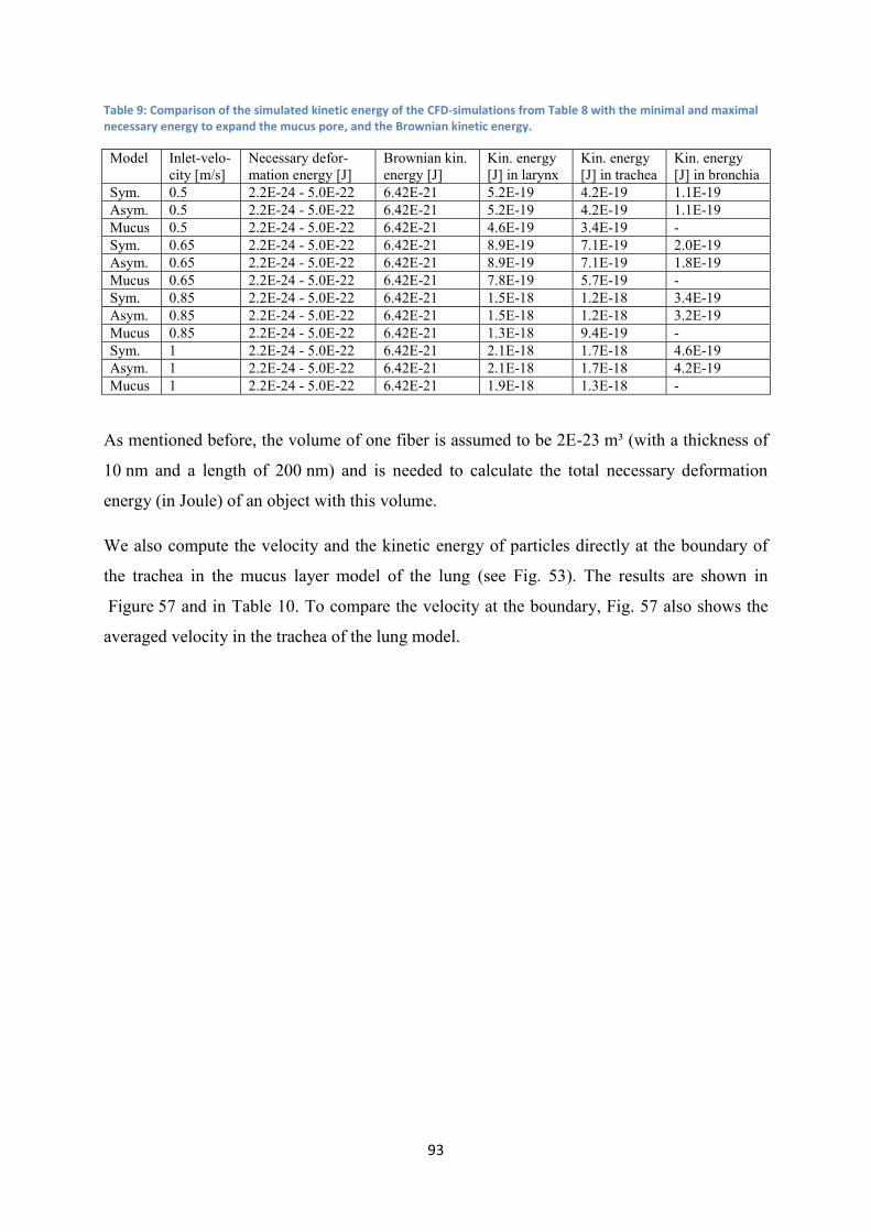
93

Table 9: Comparison of the simulated kinetic energy of the CFD-simulations from Table 8 with the minimal and maximal necessary energy to expand the mucus pore, and the Brownian kinetic energy.

Model Inlet-velo-

city [m/s]

Necessary defor-

mation energy [J]

Brownian kin.

energy [J]

Kin. energy

[J] in larynx

Kin. energy

[J] in trachea

Kin. energy

[J] in bronchia

Sym. 0.5 2.2E-24 - 5.0E-22 6.42E-21 5.2E-19 4.2E-19 1.1E-19

Asym. 0.5 2.2E-24 - 5.0E-22 6.42E-21 5.2E-19 4.2E-19 1.1E-19

Mucus 0.5 2.2E-24 - 5.0E-22 6.42E-21 4.6E-19 3.4E-19 -

Sym. 0.65 2.2E-24 - 5.0E-22 6.42E-21 8.9E-19 7.1E-19 2.0E-19

Asym. 0.65 2.2E-24 - 5.0E-22 6.42E-21 8.9E-19 7.1E-19 1.8E-19

Mucus 0.65 2.2E-24 - 5.0E-22 6.42E-21 7.8E-19 5.7E-19 -

Sym. 0.85 2.2E-24 - 5.0E-22 6.42E-21 1.5E-18 1.2E-18 3.4E-19

Asym. 0.85 2.2E-24 - 5.0E-22 6.42E-21 1.5E-18 1.2E-18 3.2E-19

Mucus 0.85 2.2E-24 - 5.0E-22 6.42E-21 1.3E-18 9.4E-19 -

Sym. 1 2.2E-24 - 5.0E-22 6.42E-21 2.1E-18 1.7E-18 4.6E-19

Asym. 1 2.2E-24 - 5.0E-22 6.42E-21 2.1E-18 1.7E-18 4.2E-19

Mucus 1 2.2E-24 - 5.0E-22 6.42E-21 1.9E-18 1.3E-18 -

As mentioned before, the volume of one fiber is assumed to be 2E-23 m³ (with a thickness of

10 nm and a length of 200 nm) and is needed to calculate the total necessary deformation

energy (in Joule) of an object with this volume.

We also compute the velocity and the kinetic energy of particles directly at the boundary of

the trachea in the mucus layer model of the lung (see Fig. 53). The results are shown in

Figure 57 and in Table 10. To compare the velocity at the boundary, Fig. 57 also shows the

averaged velocity in the trachea of the lung model.

94

Figure 57: Velocity at the boundary of the trachea (red line) and averaged velocity in the trachea (blue bullets) in the mucus layer model of the lung with an inlet velocity of 1 m/s (lower z-values for the upper trachea and higher z-values

for the lower trachea).

The velocity at the boundary is zero, if the mucus layer is present (see sketch in Fig. 57 for the

red intersection line at the boundary). Contrary, the averaged velocity at the position, where

the mucus layer is reducing the tube diameter is higher than the inlet velocity, due to the

reduction of the diameter and the resulting conservation of the volume rate. However, the

velocity of the air at the mucus layer is zero (no-slip boundary condition with a velocity of

zero at the boundaries), so the particles, which are being transported by this fluid flow, will

impact at the mucus layer in case of deceleration, due to their inertia. The resulting kinetic

energy is shown in Table 10.

95

Table 10: Comparison of the simulated kinetic energy from the CFD-simulations of the mucus layer model (velocity at the boundary of the trachea) with the minimal and maximal necessary energy to expand the mucus pore, and the Brownian kinetic energy.

Model Inlet-velo-

city [m/s]

Necessary defor-

mation energy [J]

Brownian kin.

energy [J]

Velocity [m/s]

at the boundary of

the trachea

Kin. energy [J] at

the boundary of

the trachea

Mucus 0.5 2.2E-24 - 5.0E-22 6.42E-21 0.04 3.4E-21

Mucus 0.65 2.2E-24 - 5.0E-22 6.42E-21 0.05 5.2E-21

Mucus 0.85 2.2E-24 - 5.0E-22 6.42E-21 0.07 1.0E-20

Mucus 1 2.2E-24 - 5.0E-22 6.42E-21 0.08 1.3E-20

The kinetic energy of inhaled particles is significantly higher than the necessary deformation

energy, whereat the former should be higher, if bigger particles will be inhaled due to the

mass dependency of the kinetic energy (see Eq. 34). Also the Brownian diffusive energy of a

particle at 37 °C, which is generally lower than the kinetic energy of a 200nm-particle in an

air stream, is still high enough for a particle to penetrate the mucus layer. We showed that, the

particle size should be high enough to achieve the necessary deformation energy after

impaction at the mucus layer and to depose in the bronchial regions, but only extremely small

particles yield in a Brownian diffusive energy, which is high enough to expand the pores. So,

as mentioned before, particles in the µm-range should be inhaled and release smaller

nanoparticles after impaction, to achieve a penetration of the mucus layer by diffusion.

However, it is possible for a particle, which is bigger than the mucus pore (distance between

two mucin fibers), to pass this pore by Brownian motion or inhalation without applying an

external force. Although, the mucin fibers have to be very thin (10 nm) to yield the necessary

deformation after applying relatively low energies, already particles with a diameter of 80 nm

and a velocity of 0.06 m/s achieve the necessary kinetic energy (with the mentioned

assumptions: fiber thickness of 10 nm, fiber length of 200 nm, and a Young´s modulus of

100 Pa). So, future investigations should deal with the simulation of the necessary

deformation energy of mucin fibers with different thicknesses, lengths, and Young´s moduli

and also considering various pore and particle sizes. Nevertheless, inhaling particles with a

size of several micrometers, which are releasing smaller nanoparticles -after impaction on the

mucus surface-, could be a very efficient way to deliver drugs and therapeutics to the lung

epithelial.

96

6.3 Conclusions

The air flow simulations of various upper lung models with four different inlet velocities

showed that, the resulting kinetic energy is high enough to deform the mucin fibers in a way,

that allows deposed particles to penetrate the mucus pores. So, under the given assumptions

(fiber length and thickness, rheological and mechanical properties), it is possible for a particle

to pass the mucus pore -at the interface between mucus and breathing air- after being inhaled

and impacting on the mucus layer. We showed, that there is a higher accumulation in the right

bronchia, due to the asymmetrical structure of the upper airways and the resulting lower

velocity, as it is in accordance with literature. The loss of velocity in the bronchi is also in

good agreement with literature and lies at approx. 50 %. In the mucus model of the lung,

where we modeled the mucus layer as a periodic restriction of the tube diameter, the velocity

near to the boundary is almost zero, but nevertheless high enough to yield a sufficiently high

kinetic energy. In addition, we showed a sufficiently high Brownian diffusive energy to

penetrate the mucus pores by passive Brownian motion. Finally, we can conclude, that

microparticles, which are inhaled, penetrate the mucus surface by impaction and then, after

being dispersed in extremely small nanoparticles, pass the mucus pores by Brownian diffusion

to distribute within the mucus network.

97

7 Fluorescence Recovery after Photobleaching (FRAP) for Studying

Particle-Mucus Interactions

7.1 Introduction

The determination of the fluorescence of human pulmonary mucus and polystyrene particles

after photobleaching is a very efficient way to measure the diffusivity of these particles over a

longer time range (720 s) and larger distances. FRAP means hereby a complete vanishing of

the fluorescence at a certain time (photobleaching), after which the recovery of the

fluorescence of both investigated materials will be measured, using a confocal laser

microscope [69].

The advantages of this method obviously are the very long time range and the large area, in

which the bleaching and fluorescence measurements take place, but also the possibility to

investigate the particle diffusivity on the one hand and similarly the structure of the mucus on

the other hand. One disadvantage is certainly, that the particle diffusion in the z-direction

cannot be determined. So, similar to particle tracking experiments, the diffusion in three

dimensions will be interpreted as a projected two-dimensional diffusion. However, as being

applied in [14], the 3D-MSD will be determined to be the 3/2-fold of the projected 2D-MSD.

There are also several problems, appearing during the FRAP-experiments, which are

emerging air bubbles, the adhesion of particles at the cover glass, and the missing clear

interface between particles and mucus. To avoid these problems, the particle-mucus mixture

has to be vortexed before and we used a relatively high particle concentration of 2.4% (v/v).

98

7.2 Materials & Methods

Native porcine pulmonary mucus was obtained from the tracheas of slaughtered pigs by

cutting the trachea and isolating approximately 10 cm of windpipe. The tracheas were stored

on ice for mucus extraction and prior to this extraction procedure, the tracheas were cut in half

longitudinally. The mucus was gently scratched from the luminal surface (approximately

100−300 μL of mucus per sample). The frozen mucus samples were thawed at 4 °C the day

prior to FRAP experiments. The following day, the samples reached room temperature and

thereafter 60 μL of mucus was mixed with 1.5 μL of the carboxylated green-fluorescent

polystyrene microsphere particle dispersions. The samples were then transferred into adhesive

gastight sealing chambers (Gene Frame, Thermo Scientific), and sealed with cover slides. The

FRAP experiments were conducted using a LSM 710 Axio Observer confocal laser scanning

microscope (Zeiss, Germany) with an Apochromat 40×1.1 objective equipped with a 488 nm

laser (LASOS RMC 7812 Z2). The stained mucus was detected in the green channel

(excitation 488 nm, detection 467−554 nm) and the fluorescent nanoparticles in the red

channel (excitation 561 nm, detection 624−707 nm). The sample temperature was maintained

at 37 °C. A time-series analysis was programmed with the following settings: Prebleaching

images were recorded at 2% laser transmission, immediately followed by bleaching with the

laser transmission set at 100%, and a postbleaching recovery for a duration of 760 s at a frame

rate of 30 frames per minute with the laser transmission again set at 2%. The fluorescence

intensity after bleaching was defined as zero, and the intensity at t = 0 was subtracted from all

values. The intensity values were normalized by dividing each obtained value by the

difference between the intensities prior to and directly after bleaching [69].

99

7.3 Imaging and Evaluation

7.3.1 Imaging of the particle-mucus interaction

Figure 58 shows the fluorescence imaging, using the confocal laser microscope, with the

green labeled mucus and the red labeled particles. Most of the particles are trapped in the

mucus cells, but nevertheless we see a lot of rapid particle movement in the video sequence of

these images . However, this rapid particle movement takes place in very small length scales

and therefore, the diffusivity of the particles in mucus seems to be extremely restricted. This

restricted diffusion is also obvious in Figure 60 and 61, where the fluorescence intensity

seems to approximate to a constant value for longer time scales. As shown in the passive

microrheology experiments in section 5.2.2 (Figure 42 and supplementary material) and in the

FRAP-experiments (Fig. 60 and 61), the MSD and the fluorescence intensity, respectively,

approximates to a constant value, which let us conclude, that the particle diffusion in mucus is

totally restricted for longer time and length scales. So, the MSD in particle tracking

experiments, respectively the fluorescence intensity in FRAP-experiments, can be easily fitted

and predicted by numerical simulations with pM = 0 (r = 1), as well as by analytic

approximations (see Eq. 7 in section 4.1.2).

100

Figure 58: Four different mucus samples (green area) with interacting nanoparticles (red labeled regions).

7.3.2 Evaluation of the particle diffusivity in mucus

To calculate the diffusivity of particles with a diameter of 100 nm in human pulmonary

mucus, we use a scaffold with totally 19 regions (see Fig. 59). Here, the regions #1-#10, #16-

#19, and #14 will be bleached, whereas the remaining regions serve as control-regions. After

approx. 117 s, all regions, except the control regions, are bleached and the fluorescence

intensity is determined for 718 s.

101

Figure 59: Scaffold for the fluorescence measurements after photobleaching.

Unfortunately, most of the investigated particles are more or less trapped inside a mucus cell

and therefore it is hard to determine a long-time diffusion coefficient from the FRAP data.

The following Figure 60 shows the normalized fluorescence intensity after the photobleaching

of the regions 1-5.

1 - 10

16 - 17

18 - 19

11 - 13

14

15

10 µm

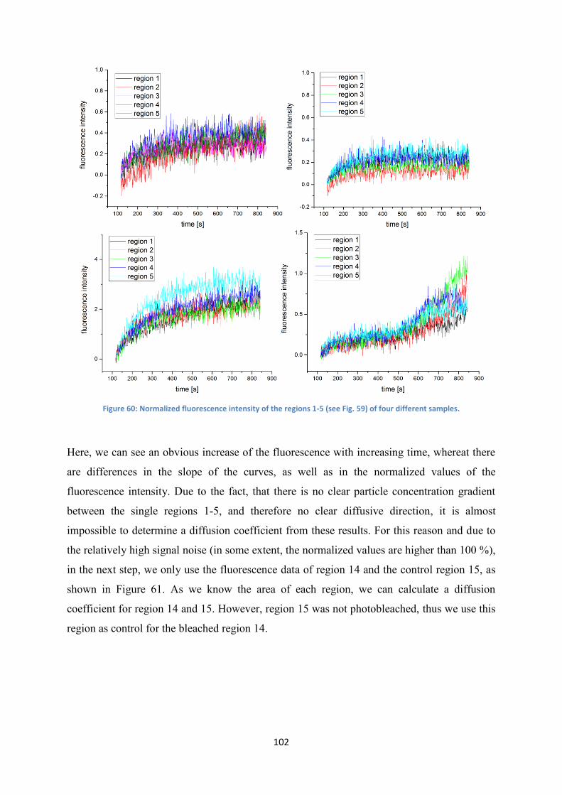
102

Figure 60: Normalized fluorescence intensity of the regions 1-5 (see Fig. 59) of four different samples.

Here, we can see an obvious increase of the fluorescence with increasing time, whereat there

are differences in the slope of the curves, as well as in the normalized values of the

fluorescence intensity. Due to the fact, that there is no clear particle concentration gradient

between the single regions 1-5, and therefore no clear diffusive direction, it is almost

impossible to determine a diffusion coefficient from these results. For this reason and due to

the relatively high signal noise (in some extent, the normalized values are higher than 100 %),

in the next step, we only use the fluorescence data of region 14 and the control region 15, as

shown in Figure 61. As we know the area of each region, we can calculate a diffusion

coefficient for region 14 and 15. However, region 15 was not photobleached, thus we use this

region as control for the bleached region 14.

103

Figure 61: Normalized fluorescence intensity of the regions 14 and 15 (see Fig. 59) of four different samples.

Here, again the differences in the shape of the curves and the normalized values are obvious,

but in particular, the results from the samples in the upper row of Figure 61 (#1 and #2 in

Table 11) are well suited to calculate a diffusion coefficient, because there is almost no

increase of the fluorescence intensity in the control region (region 15). Nevertheless, the

normalized value of the fluorescence intensity in region 14 of sample #3 (lower left Figure) is

mostly higher than one. In this case, there is a higher fluorescence intensity of the particles

than prior to the photobleaching. Subsequently, after the photobleaching there are particles

diffusing in the z-direction into the bleached area, leading to an increase of the fluorescence

intensity. Consequently, we have to consider this three-dimensional diffusion in the two-

dimensional experimental setting.

In Table 11 the calculated diffusion coefficients in [intensity µm-2

] after totally 835 s for the

regions 14 and 15, and the difference between these two regions are shown. To reduce the

diffusive effects of particles, moving in the z-direction, we have to use the difference of

intensity between region 14 and the control region 15.

104

A possibility to consider the diffusion of particles in the z-direction is to calculate the 3D-

diffusion from the projected 2D-diffusion (see Suh et al. [14]), as it is shown for region 14.

The values in brackets show the time-dependent diffusion coefficient in [intensity µm-2

s-1

].

Table 11: Diffusion coefficients after 835 s (time-dependent ones in brackets) from the fluorescence recovery after photobleaching in region 14 and 15, as well as the difference between these regions to reduce diffusive effects from particles moving in the z-direction, and the calculated 3D-diffusion from the projected 2D-diffusion in region 14 to consider the diffusion of particles in the z-direction. The upper four rows are calculated with the normalized values of the fluorescence intensity (n.).

Sample Region 14 Region 15 Difference Region 14 (3D)

#1 (15D) n. 6.9E-4 (9.5E-7) 3.7E-3 (5.1E-6) -3.0E-3 (4.2E-6) 1.0E-3 (1.4E-6)

#2 (21A) n. 6.8E-4 (9.4E-7) 1.1E-3 (1.5E-6) -4.2E-4(-5.8E-7) 1.0E-3 (1.4E-6)

#3 (21B) n. 6.6E-3 (9.1E-6) 6.5E-2 (9.0E-5) -5.8E-2 (-8.1E-5) 9.9E-3 (1.4E-5)

#4 (21D) n. 1.6E-3 (2.1E-6) 4.6E-2 (6.3E-5) -4.4E-2 (-6.1E-5) 2.4E-3 (3.3E-6)

#1 (15D) 6.2E-3 (8.6E-6) 3.7E-3 (5.1E-6) 2.5E-3 (3.5E-6) 9.3E-3 (1.3E-5)

#2 (21A) 5.9E-3 (8.1E-6) 1.1E-3 (1.5E-6) 4.8E-3 (6.6E-6) 8.9E-3 (1.2E-5)

#3 (21B) 3.0E-2 (4.2E-5) 6.5E-2 (9.0E-5) -3.5E-2 (-4.8E-5) 4.5E-2 (6.2E-5)

#4 (21D) 9.9E-3 (1.4E-5) 4.6E-2 (6.3E-5) -3.6E-2 (-5.0E-5) 1.5E-2 (2.1E-5)

As shown, in all samples, the area-specific diffusivity in the control region 15 is significantly

higher than in the bleached region 14, if the values of the fluorescence intensity are

normalized. If the values are not normalized, only in the samples #3 and #4 the diffusivity in

the control region 15 is significantly higher than in the bleached region 14. We expected the

intensity in the control region to be constant at a value of zero, due to the assumption, that as

much particles move in this region as particles move out of the region. As shown in Figure 61,

this assumption is only valid for the samples #1 and #2.

Contrary to the simulations of Brownian diffusion (see chapter 4), in these experiments, the

subdiffusive behavior of particles in mucus is not a transient effect. So, depending on the

experimental setting, the diffusion of particles is totally trapped -reflection probability r = 1 in

our simulations and a constant MSD, respectively fluorescence intensity (see sample #1)-,

subdiffusive -reflection probability r < 1 and a MSD, respectively fluorescence intensity, ~ α

with α < 1 (see sample #2)- or transient subdiffusive.

105

7.4 Conclusions

The fluorescence recovery after photobleaching is a good method to visualize the extremely

heterogeneous and complex structure of mucus. Hence, the particles are mostly trapped inside

the single mucus cells and their diffusion is extremely confined, which is expressed by the

constant fluorescence values (lower than the initial value before bleaching) even after

15 minutes. The calculation of the diffusivity of 100 nm-particles in mucus showed, that it is

very hard to quantitatively describe the diffusion in mucus by this method, due to the 2D-

projection of a 3D-movement, as it is also obvious in particle tracking experiments. So, there

are several methods to determine the diffusivity of particles in mucus, leading to different

conclusions about the type of diffusion (totally trapped, subdiffusive or transient

subdiffusive).

106

8 Assumptions and Hypotheses

To simulate the Brownian motion of particles in a confined geometry, we used a simplified

cell-aperture model, which we abstracted to a cavity-membrane model with permeable

membranes and certain transmission probabilities. The only essential parameters, needed in

this model, are the diffusion coefficients for the short and long time limits, the size of the

cavity edge, respectively the distance between the membranes, and the permeability of the

membranes. We assumed a regular array of cells and windows, respectively membranes, and

mixed boundary conditions to simulate the mucus structure and its properties. So, as we used

an isotropic geometry with permeable membranes, the complex model for simulating

Brownian motion of particles in a three-dimensional geometry can be reduced to a one-

dimensional membrane model. However, we simulated the (Fickian) diffusion of particles,

based on concentration gradients to compare it with two (Brownian and Fickian) diffusion

models, based on permeable membranes. In case of the Fickian diffusion, based on

concentration gradients, we used a two-dimensional cell-window, respectively cell-

membrane, model with an array of cells, connected by windows, membranes respectively.

only in one direction. In our diffusion models, we assumed the fluid to be purely viscous, the

membranes and walls to be rigid, and particles, respectively mucus, without any electrostatic

or chemical interactive properties. Nevertheless, we are able to simulate the diffusion of

particles with different properties and diameters in mucus from different sources, as well as to

predict the time to penetrate a certain distance in the mucus layer. To simulate the

concentration-gradient based diffusion, we assumed an equal distribution of particles as

diluted species at one boundary and vanishing particles at the opposite boundary in direction

of diffusion. The windows in this model represent the mucus pores, which are voids in the

mucin fiber network. To determine the necessary deformation energy of such a mucin fiber to

achieve a certain expansion of the mentioned void, we assumed the fiber to be an elastic beam

with a specified Young´s modulus, yielded from rheometry and optical tweezer experiments.

One edge of the fiber was assumed to be fixed, whereas the opposite edge was deflected in the

y-direction or deformed in the x-direction. Consequently, the void between two ideally

identical fibers was expanded in a way, that allows a particle to pass through. The assumption

of the fiber, being an elastic beam, is not that realistic, as the mucin fibers are more

viscoelastic and semiflexible, but in a first approach it is valid to estimate the deformation

energy.

107

To verify, if the particle impact is high enough to reach the needed deformation of the fibers,

we simulated the convective air flow in different lung models. We used various inlet

velocities, which result in realistic flow rates during the inhalation of an aerosol. As we

assumed an overdamped movement of particles in this aerosol and due to the vanishing

particle mass, we neglected the particle movement in the convective air flow. Subsequently,

we calculated the kinetic energy of the particles by computing the air velocity in different

regions of our lung models. This assumption is only valid for particles with a negligible

particle friction force in the air stream. However, our model is very simplified, concerning the

particle-air interactions, but nevertheless we used a nearly realistic asymmetrical lung model

with comparable inlet flow rates and pressure conditions. So, we are able to determine the

kinetic energy of an inhaled particle and compare this energy with the necessary deformation

energy of a mucin fiber, considering measured Young`s moduli.

108

9 Summary and Outlook

We developed four diffusion models to simulate the particle movement through a cell array,

representing the mucus network. We achieved realistic diffusion models by assuming the

mucus to be an array of cells with periodic open windows or with periodic diffusion barriers,

each barrier provided with a different diffusion coefficient. Both models were compared with

a one-dimensional model, based on periodic permeable membranes, whereat we compared the

size of the open windows with the permeability parameter and the diffusion coefficient of the

diffusive barriers with the effective diffusion coefficient, respectively. Two one-dimensional

models are based on permeable membranes with a certain permeability parameter and either

random or constant permeation probabilities of the particles for each investigated time step.

The two-dimensional models are based on a concentration gradient and with particles as

diluted species, contrary to the random particle walk, which is assumed in the one-

dimensional models. The two-dimensional models can be interpreted more easily, since they

are based on measureable parameters, such as the size of a mucus cell and of the pores in the

mucus network.

We explained the reported subdiffusion of particles in mucus by simulating the Brownian

diffusion of particles in a confined geometry, made from permeable membranes in analogy to

mixed boundary conditions. A heuristic analytic approximation formula was substantiated by

numerical simulations. The applied model predicted a normal diffusive behavior at very short

τ → 0 and long times τ → ∞, as it is observed in several particle tracking experiments. In

between these time scales, the "subdiffusive" regime appeared to be a transient effect,

MSD ~ τα, α < 1. The only necessary parameters in the model are the diffusion-coefficients D0

and Deff, and the distance between the permeable membranes L. Our results were in

agreement with published experimental data for realistic assumptions of these parameters. We

showed, that particles with a diameter lower than 40 nm are able to pass through a mucus

layer with a thickness of approx. 55 µm (interstitial fluid viscosity η = 7 mPas) within a

clearance time of 15 min by passive Brownian motion.

Simulations of the probability density function of the particle displacement showed that, even

500nm-particles pass a specific mucus layer thickness. Consequently, these big particles are

not totally restricted in their movement. None of the investigated uncoated and coated

particles with different sizes are totally trapped inside a mucus cell, but their diffusivity is

significantly different.

109

Some of the 100nm-particles are able to overcome a distance of 10 µm already after

100 seconds. After calculating the mean passage time, we concluded, that there is no

possibility for any of the investigated particles to overcome a mucus layer of 55 µm thickness

within a mucus turnover time of 15 minutes by passive Brownian motion. However, in case of

cystic fibrosis mucus, this turnover time is significantly higher. Subsequently, mucus from

patients with lung disease can be passed by some particles, if the clearance time is comparable

to the mean passage time. Nevertheless, only particles with a diameter of below 300 nm are

able to overcome a fluid layer with a viscosity of 1 mPas, respectively the maximal viscosity

of a fluid to enable a particle displacement (100nm-particle) of 55 µm within 15 minutes is

3 mPas. Consequently, there have to be some active particle motion processes to achieve a

faster particle penetration of mucus by affecting the particle displacement.

To achieve a better insight in the system, an analytic relation between the permeability pM

in s-1/2

and the effective diffusion coefficient Deff(pM) will be helpful (see Fig. 10 and Fig. 14).

The model predicted normal diffusion for short and long times and therefore, further

experiments with a wider range of time lag in the MSD(τ)-data could verify our predictions.

Additionally, an experimental validation of the Gaussian shape of the probability density

function of the particle displacement still remains missing. However, we are able to simulate

the probability density function of the particle displacement in mucus by using the assumed

values for the three essential parameters Deff(pM), D0, and L.

We investigated the similarities and differences in the viscoelastic (macro- and

microrheological) properties of mucus from pulmonary and intestinal regions of healthy pigs.

Our results revealed significant differences between respiratory and intestinal mucus, in the

macro- and microscale as well. The measured Young´s modulus was used to simulate the

necessary deformation energy of a mucus fiber. This fiber deformation yielded in a pore

expansion, which allows the particle to pass the mucus layer. The deformation of a mucin

fiber can be achieved either by impaction, due to convective particle flow, or by the Brownian

diffusive energy. The kinetic energy of an inhaled particle in a convective air flow was

computed by simulating the air dynamics in three different lung models. We showed, that the

Brownian diffusive energy of a particle, as well as the kinetic energy of an inhaled particle,

are high enough to yield a sufficient fiber deformation for the given assumptions. This

deformation results in a pore expansion, which allows the particle to pass the mucus pore.

110

Future investigations of the possibility for particles in a convective flow to penetrate the

mucus layer by impaction should deal with a variation of the mucin fiber parameters, such as

the Young`s modulus, the Poisson number, the density, the length and thickness of the fiber,

and also the pore size, as well as the particle size. Furthermore, time-dependent CFD- and

deformation-simulations should be executed, as well as flow simulations with integrated

particle deposition analysis.

In the last section of this work, we showed by applying fluorescence recovery methods, that

particles are mostly trapped inside the mucus structure, as it is also obvious in some particle

tracking experiments. Although, the particles are moving rapidly inside a mucus cell, this

displacement is within an extremely small area and time lag. Nevertheless, we could

discriminate between three different types of diffusion as these are: totally trapped diffusion,

subdiffusion, and transient subdiffusion. All of these diffusion types have been detected in the

presented experiments and can be predicted by our model simulations.

Due to the projection of the three-dimensional particle movement in mucus to a two-

dimensional dataset in experiments (particle tracking and FRAP), a simulation of the

projected particle movement in the third dimension should be helpful to quantitatively

describe the particle diffusion in non-isotropic materials. However, we must not simulate a 3D

diffusion, as we are able to simulate the particle movement through a sequence of permeable

membranes in one dimension. By assuming different values of the permeability of the

membrane, the distance between the membranes, and the diffusion coefficient in the short

time limit, we are able to predict the long-time diffusion in more than one dimension for

isotropic models. Subsequently, it is also not necessary to consider physical and chemical

properties of the mucus and the particles, as we can put these properties into the three

essential parameters Deff(pM), D0, and L.

To close this work, we can finally conclude, that it is possible to simulate the particle

impaction at the mucus layer, due to convective air flow, and to compute the resulting kinetic

energy, since we developed realistic models of the upper lung. This impaction leads to a pore

expansion, which allows the particle to penetrate into the mucus network for given

assumptions on the mucin fiber geometry and its mechanical and rheological properties. We

developed realistic diffusion models to predict the particle movement inside the mucus

structure and to explain the appearing transient "subdiffusive" behavior of the particles.

111

10 References

[1] Gehr, P., C. Mühlfeld, B. Rothen-Rutishauser, and F. Blank, 2010. Particle-Lung Interactions

Second Edition. informa Healthcare.

[2] Serda, R. E., 2013. Mass Transport of Nanocarriers. CRC Press.

[3] Lai, S. K., Y.-Y. Wang, D. Wirtz, and J. Hanes, 2009. Micro and Macrorheology of mucus. Adv

Drug Delivery 61:86–100.

[4] Khanvilkar, K., M. D. Donovan, and D. R. Flanagan, 2001. Drug Transfer through mucus.

Advanced Drug Delivery Reviews 48:173–193.

[5] Cu, Y., and W. M. Saltzmann, 2009. Mathematical modeling of molecular diffusion through

mucus. Adv Drug Delivery 61:101–114.

[6] Lieleg, O., and K. Ribbeck, 2011. Biological Hydrogels as Selective Diffusion Barriers. Trends

Cell Biology 21:543 – 551.

[7] Lai, S. K., Y.-Y.Wang, and J. Hanes, 2009. Mucus-penetrating nanoparticles for drug and gene

delivery to mucosal tissues. Advanced Drug Delivery Reviews 61:158–171.

[8] Kirch, J., A. Schneider, B. Abou, A. Hopf, U. F. Schaefer, M. Schneider, C. Schall, C. Wagner,

and C.-M. Lehr, 2012. Optical tweezers reveal relationship between microstructure and nanoparticle

penetration of pulmonary mucus. PNAS 109:18355.

[9] Sigurdsson, H. H., J. Kirch, and C.-M. Lehr, 2013. Mucus as a barrier to lipophilic drugs.

International Journal of Pharmaceutics 453:56–64.

[10] Boegh, M., and H. M. Nielsen, 2015. Mucus as a Barrier to Drug Delivery Understanding and

Mimicking the Barrier Properties. Basic & Clinical Pharmacology & Toxicology 116:179–186.

[11] Schuster, B. S., J. S. Suk, G. F. Woodworth, and J. Hanes, 2013. Nanoparticle diffusion in

respiratory mucus from humans without lung disease. Biomaterials 34:3439–3446.

[12] Suk, J. S., Q. Xu, N. Kim, J. Hanes, and L. M. Ensign, 2016. PEGylation as a strategy for

improving nanoparticle-based drug and gene delivery. Advanced Drug Delivery Reviews 99:28–51.

[13] Sanders, N. N., S. C. de Smedt, E. van Rompaey, P. Simoens, F. de Baets, and J. Demeester,

2000. Cystic Fibrosis Sputum: A Barrier to the Transport of Nanospheres. Am J Respir Crit Care Med

162:1905–1911.

[14] Suh, J., M. Dawson, and J. Hanes, 2005. Real-time multiple particle tracking: applications to drug

and gene delivery. Advanced Drug Delivery Reviews 57:63–78.

[15] Sung, J. C., B. L. Pulliam, and D. A. Edwards, 2007. Nanoparticles for Drug Delivery to the

Lungs. Trends in Biotechnology 25:563–570.

[16] Tang, B. C., M. Dawson, S. K. Lai, Y.-Y. Wang, J. S. Suk, M. Yang, P. Zeitlin, M. P. Boylee, J.

Fua, and J. Hanes, 2009. Biodegradable polymer nanoparticles that rapidly penetrate the human mucus

barrier. PNAS 106:19268–19273.

112

[17] Suk, J. S., A. J. Kim, K. Trehan, C. S. Schneider, L. Cebotaru, O. M. Woodward, N. J. Boylan,

M. P. Boyle, S. K. Lai, W. B. Guggino, and J. Hanes, 2014. Lung gene therapy with highly compacted

DNA nanoparticles that overcome the mucus barrier. Journal of Controlled Release 178:8–17.

[18] Lai, S. K., D. E. O’Hanlon, S. Harrold, S. T. Man, Y.-Y.Wang, R. Cone, and J. Hanes, 2007.

Rapid transport of large polymeric nanoparticles in fresh undiluted human mucus. PNAS 104:1482 –

1487.

[19] Forier, K., A.-S. Messiaen, K. Raemdonck, H. Deschout, J. Rejman, F. De Baets, H. Nelis, S. C.

De Smedt, J. Demeester, T. Coenye, and K. Braeckmans, 2013. Transport of nanoparticles in cystic

fibrosis sputum and bacterial biofilms by single-particle tracking microscopy. Nanomedicine 8:935–

949.

[20] Lieleg, O., I. Vladescu, and K. Ribbeck, 2010. Characterization of Particle Translocation through

Mucin Hydrogels. Biophysical Journal 98:1782 – 1789.

[21] Forier, K., K. Raemdonck, S. C. De Smedt, J. Demeester, T. Coenye, and K. Braeckmans, 2014.

Lipid and polymer nanoparticles for drug delivery to bacterial biofilms. Journal of Controlled Release

190:607–623.

[22] Kirch, J., M. Guenther, N. Doshi, U. F. Schaefer, M. Schneider, S. Mitragotri, and C.-M. Lehr,

2012. Mucociliary clearance of micro- and nanoparticles is independent of size, shape and charge: an

ex vivo and in silico approach. Journal of Controlled Release 159:128–134.

[23] Bhat, P. G., D. R. Flanagan, and M. D. Donovan, 1996. Drug Diffusion through Cystic Fibrotic

Mucus: Steady-State Permeation, Rheologic Properties, and Glycoprotein Morphology. Journal of

Pharmaceutical Sciences 85:624–630.

[24] Broughton-Head, V. J., J. R. Smith, J. Shur, and J. K. Shute, 2007. Actin limits enhancement of

nanoparticle diffusion through cystic fibrosis sputum by mucolytics. Pulmonary Pharmacology &

Therapeutics 20:708–717.

[25] Regnis, J. A., M. Robinson, D. L. Bailey, P. Cook, P. Hooper, H.-K. Chan, I. Gonda, G.

Bautovich, and P. T. P. BYE, 1994. Mucociliary Clearance in Patients with Cystic Fibrosis and in

Normal Subjects. Am J Respir Crit Care Med 150:66–71.

[26] Dudko, O. K., A. M. Berezhkovskii, and G. H. Weiss, 2004. Diffusion in the presence of

periodically spaced permeable membranes. The Journal of Chemical Physics 121:1–6.

[27] Dudko, O. K., A. M. Berezhkovskii, and G. H. Weiss, 2005. Time-Dependent Diffusion

Coefficients in Periodic Porous Materials. Journal of Physical Chemistry B 109:21296–21299.

[28] Ditlevsen, S., and A. Samson, 2013. Stochastic Biomathematical Models, Chapter 1 (Introduction

to Stochastic Models in Biology). Springer-Verlag.

[29] Nelson, E., 2001. Dynamical Theories of Brownian Motion. Princeton University Press.

[30] Muermann, M., 2014. Wahrscheinlichkeitstheorie und Stochastische Prozesse. Springer.

[31] Harrison, J. M., 1985. Brownian Motion and Stochastic Flow Systems. John Wiley & Sons.

[32] Beichelt, F., 1997. Stochastische Prozesse für Ingenieure. B.G. Teubner-Verlag.

113

[33] Behrends, E., 2013. Markovprozesse und Stochastische Differentialgleichungen. Springer-Verlag.

[34] Schwetlick, H., 1997. PC-Messtechnik. Vieweg-Verlag.

[35] Norris, D. A., and P. J. Sinko, 1997. Effect of Size, Surface Charge, and Hydrophobicity on the

Translocation of Polystyrene Microspheres Through Gastrointestinal Mucin. Journal of Applied

Polymer Science 63:14811492.

[36] Saltzmann, W. M., 2001. Drug Delivery. Oxford University Press.

[37] Erickson, A. M., B. I. Henry, J. M. Murray, P. J. Klasse, and C. N. Angstmann, 2015. Predicting

First Traversal Times for Virions and Nanoparticles in Mucus with Slowed Diffusion. Biophysical

Journal 109:164–172.

[38] Berezhkovskii, A. M., M. I. Monine, C. B. Muratov, and S. Y. Shvartsman, 2006.

Homogenization of boundary conditions for surfaces with regular arrays of traps. The Journal of

Chemical Physics 124:1–3.

[39] Makhnovskii, Y., A. Berezhkovskii, and V. Zitserman, 2010. Diffusion in a tube of alternating

diameter. Chemical Physics 367:110–114.

[40] Berezhkovskii, A. M., L. Dagdug, and S. M. Bezrukov, 2014. Discriminating between

Anomalous Diffusion and Transient Behavior in Microheterogeneous Environments. Biophysical

Journal 106:L09–L011.

[41] Berezhkovskii, A. M., L. Dagdug, and S. M. Bezrukov, 2015. Biased diffusion in three-

dimensional comb-like structures. The Journal of Chemical Physics 142:1–10.

[42] Berezhkovskii, A. M., L. Dagdug, and S. M. Bezrukov, 2014. From normal to anomalous

diffusion in comb-like structures in three dimensions. The Journal of Chemical Physics 141:1–7.

[43] Bezrukov, S., L. Schimansky-Geier, and G. Schmid, 2014. Brownian motion in confined

geometries. The European Physical Journal Special Topics 223:3021–3025.

[44] Makhnovskii, Y. A., A. M. Berezhkovskii, and V. Y. Zitserman, 2009. Time-dependent diffusion

in tubes with periodic partitions. The Journal of Chemical Physics 131:1–5.

[45] Boukari, H., B. Brichacek, P. Stratton, S. F. Mahoney, J. D. Lifson, L. Margolis, and R. Nossal,

2009. Movements of HIV-Virions in Human Cervical Mucus. Biomacromolecules 10:2482–2488.

[46] Banks, D. S., C. Tressler, R. D. Peters, F. H¨ofling, and C. Fradin, 2016. Characterizing

anomalous diffusion in crowded polymer solutions and gels over decades in time with variable-

lengthscale fluorescence correlation spectroscopy. Soft Matter 18:1–14.

[47] Weeks, E. R., and D. A. Weitz, 2002. Subdiffusion and the cage effect studied near the colloidal

glass transition. Chemical Physics 284:361–367.

[48] Martin, D. S., M. B. Forstner, and J. A. Käs, 2002. Apparent Subdiffusion Inherent to Single

Particle Tracking. Biophysical Journal 83:2109–2117.

[49] Michalet, X., 2010. Mean Square Displacement Analysis of Single-Particle Trajectories with

Localization Error: Brownian Motion in Isotropic Medium. Physical Review E: Statistical, Nonlinear,

and Soft Matter Physics 82:1–26.

114

[50] Hansing, J., C. Ciemer, W. K. Kim, X. Zhang, J. E. DeRouchey, and R. R. Netz, 2016.

Nanoparticle filtering in charged hydrogels: Effects of particle size, charge asymmetry and salt

concentration. The European Physical Journal E 39:53.

[51] Cicuta, P., and A. M. Donald, 2007. Microrheology: a review of the method and applications.

Soft Matter 3:1449–1455.

[52] Gillespie, D. T., and E. Seitaridou, 2013. Simple Brownian Diffusion. Oxford University Press.

[53] Islam, M. A., 2004. Einstein Smoluchowski Diffusion Equation: A Discussion. Physica Scripta

70:120–125.

[54] Kusumi, A., Y. Sako, and M. Yamamoto, 1993. Confined Lateral Diffusion of Membrane

Receptors as Studied by Single Particle Tracking (Nanovid Microscopy). Effects of Calcium-induced

Differentiation in Cultured Epithelial Cells. Biophysical Journal 65:2021–2040.

[55] Lucena, D., D. Tkachenko, K. Nelissen, V. Misko,W. Ferreira, G. Farias, and F. Peeters, 2012.

Transition from single-file to two-dimensional diffusion of interacting particles in a quasi one-

dimensional channel. Physical Review E: Statistical, Nonlinear, and Soft Matter Physics 85:1–12.

[56] Nandi, A., D. Heinrich, and B. Lindner, 2012. Distributions of diffusion measures from a local

mean-square displacement analysis. Physical Review E: Statistical, Nonlinear, and Soft Matter Physics

86:1–13.

[57] Burada, P. S., P. Hänggi, F. Marchesoni, G. Schmid, and P. Talkner, 2009. Diffusion in Confined

Geometries. Chem Phys Chem 10:45–54.

[58] Higham, D. J., 2001. An Algorithmic Introduction to Numerical Simulation of Stochastic

Differential Equations. Society for Industrial and Applied Mathematics 43:525–546.

[59] Schuss, Z., 2013. Brownian Dynamics at Boundaries and Interfaces, volume 186. Springer.

[60] Singer, A., Z. Schuss, A. Osipov, and D. Holcman, 2008. Partially Reflected Diffusion. SIAM

Journal on Applied Mathematics 68:844/868.

[61] Bathe, K.-J., 1996. Finite Element Procedures. Prentice-Hall.

[62] http://www.fachdidaktik.physik.ethz.ch/education/AbgeschlosseneArbeiten/TJenniF_VF

initeElemente.pdf (2011)

[63] Ripplinger, 2013. Einführung in die Finite Elemente Methode

[64] Schwarz, H. R., 1980. Methode der finiten Elemente. B. G. Teubner Stuttgart.

[65] Allen, A., L. A. Sellers, and M. K. Bennett, 1987. The Gastric Mucosal Epithelial Barrier: Role of

Mucus and Fibrin. Scandinavian Journal of Gastroenterology 22:6–13.

[66] Taylor, C., A. Allen, P. W. Dettmar, and J. P. Pearson, 2004. Two rheologically different gastric

mucus secretions with different putative functions. Biochimica et Biophysica Acta 1674:131–138.

[67] Taylor, C., K. I. Draget, J. P. Pearson, and O. Smidsrd, 2005. Mucous Systems Show a Novel

Mechanical Response to Applied Deformation. Biomacromolecules 6:1524–1530.

115

[68] Kilcoyne, M., J. Q. Gerlach, M. Kane, and L. Joshi, 2012. Construction of a Natural Mucin

Microarray and Interrogation for Biologically Relevant Glyco-Epitopes. Analytical Chemistry

84:3330–3338.

[69] Murgia, X., P. Pawelzyk, U. F. Schaefer, C. Wagner, N. Willenbacher, and C.-M. Lehr, 2016.

Size-Limited Penetration of Nanoparticles into Porcine Respiratory Mucus after Aerosol Deposition.

Biomacromolecules 17:1536–1542.

[70] Lafitte, G., O. Soderman, K. Thuresson, and J. Davies, 2007. PFG-NMR Diffusometry: A Tool

for Investigating the Structure and NMR Diffusometry: A Tool Purified Pig Gastric Mucin in a and

Dynamics of Noncommercial for Investigating the Structure: Wide Range of Concentrations.

Biopolymers 86:165–175.

[71] Capitanio, M., and F. S. Pavone, 2013. Interrogating Biology with Force: Single Molecule High-

Resolution Measurements with Optical Tweezers. Biophysical Journal 105:1293–1303.

[72] Böge, A., 2011. Technische Mechanik. Vieweg-Verlag, 29 edition.

[73] https://electures.informatik.uni-freiburg.de/portal/download/.../Vorlesung_biegelinie.ppt (2010)

[74] http://www.chemie.de/lexikon/Vergleichsspannung.html.

[75] Gengenbach, T., 2012. Numerical Simulation of Particle Deposition in the Human Lungs. Ph.D.

thesis, Karlsruhe Institut für Technologie Fakultät für Mathematik.

[76] Schünke, M., E. Schulte, and U. Schumacher, 2005. Prometheus Lernatlas der Anatomie: Hals

und Innere Organe. Thieme-Verlag.

[77] Oberdörster, G., E. Oberdörster, and J. Oberdörster, 2005. Nanotoxicology: An Emerging

Discipline Evolving from Studies of Ultrafine Particles. Environmental Health Perspectives 113:823 –

839.

[78] Zhang, Z., C. Kleinstreuer, J. Donohue, and C. Kim, 2005. Comparison of micro- and nano-size

particle depositions in a human upper airway model. Journal of Aerosol Science 36:211–233.

[79] Li, Z., C. Kleinstreuer, and Z. Zhang, 2007. Simulation of airflow fields and microparticle

deposition in realistic human lung airway models. Part I & II: Airow patterns & Particle transport and

deposition. European Journal of Mechanics B/Fluids 26:632–649 & 26:650-668.

[80] http://www.spektrum.de/lexikon/biologie/atemmechanik/5742.

[81] Hinds, W. C., 1982. Aerosol Technology. John Wiley & Sons.

[82] Yu, G., Z. Zhang, and R. Lessmann, 1998. Fluid Flow and Particle Diffusion in the Human Upper

Respiratory System. Aerosol Science and Technology 28:146–158.

[83] Farkas, A, and I. Balashazy, 2008. Quantification of particle deposition in asymmetrical

tracheobronchial model geometry. Computers in Biology and Medicine 38:508–518.

[84] Liu, Y., R. So, and C. Zhang, 2002. Modeling the bifurcating flow in a human lung airway.

Journal of Biomechanics 35:465–473.

116

11 List of Abbreviations

A - barrier thickness

α - anomaly exponent

b - width of the mucin fiber

c - concentration of diluted species in a fluid

dm - mucus layer thickness

dp - size of window, pore

DL - tube diameter / characteristic dimension, length

D0 - diffusion coefficient (Stokes-Einstein)

Deff - effective diffusion coefficient

Δl - distance between the center of the curved section (during deflection) and fiber ending

Δτ - duration of discrete time step

E - Young`s modulus

EBrown - Brownian diffusive energy

Ekin - kinetic energy

εel - elastic strain

η - dynamic viscosity

F - (particle impact) force

Fext - external force

Fthermal - thermal force

FStokes - Stokes force

f - deflection

G`, G`` - elastic, viscous modulus

g - Gaussian distributed random number

γB - bronchial angle

h - height of the mucin fiber

IM - second moment of area

kB - Boltzmann constant

117

L - edge size of cell cavity / distance between membranes

l - length of the mucin fiber

M - force moment

mp - particle mass

mod - modulus function

MSD - mean squared displacement

µ - mean

µf - kinematic viscosity

N - number of time steps, iterations

n - number of observations

Np - number of particles

ν - Poisson number

p - statistical significance

pexp - pore expansion

pdf - probability density function

pl - pressure in the lung

pM - permeability

R - hydrodynamic particle radius

r - reflection probability

Re - Reynolds number

ρf - fluid density

ρp - particle density

s - curved section during deflection

St - Stokes number

σ2 - variance

σvM - von-Mises stress

σel - elastic stress

T - absolute temperature

τMC - mucociliary clearance time

118

τp - mean passage time

τ, t, s - time interval, time

u - fluid velocity

v - particle velocity

w - deformation

ω - frequency

x - (particle) position

X, S - system of random variables

ξ - standard Gaussian noise

119

12 List of Tables

1 - Examples of particle diffusion in mucus

2 - Comparison of effective diffusion coefficients from experiments and simulations

3 - Mean passage times and diffusion coefficients for various simulation parameters,

particle sizes, mucus properties, and particle coatings

4 - Examples of rheological parameters of mucus

5 - Comparison of rheological parameters of mucus from own experiments and previous

studies

6 - Examples of CFD-simulation results of particle flow and deposition in the lung

7 - CFD-steps

8 - Velocities and kinetic energies of our CFD-simulations

9 - Comparison of Brownian diffusive energy, kinetic energy of inhaled particles in the

lung, and the necessary deformation energy

10 - Comparison of Brownian diffusive energy, kinetic energy of inhaled particles at the

boundary of the trachea, and the necessary deformation energy

11 - Diffusion coefficients from FRAP-experiments

120

13 List of Figures

1 - Microscopic images of mucus

2 - Barrier properties of mucus

3 - Diffusion types in mucus

4 - Diffusion variants in mucus

5 - Mucociliary clearance

6 - Representation of the mucus model

7 - Calculated MSD and anomaly exponent from simulated Brownian diffusion

8 - Relative error between numerical and analytical solutions of Brownian diffusion

simulations

9 - Relative error versus permeability of the membranes for simulated Brownian diffusion

10 - Ratio of Deff and D0 from simulated Brownian diffusion

11 - Calculated MSD and anomaly exponent from simulated Fickian diffusion

12 - Relative error between numerical and analytical solutions of Fickian diffusion

simulations

13 - Relative error versus permeability of the membranes for simulated Fickian diffusion

14 - Ratio of Deff and D0 from simulated Fickian diffusion

15 - MSD of uncoated PS-particles in sputum from CF patients from experiments and

calculated by Brownian diffusion simulations

16 - MSD of uncoated PS-particles in sputum from CF patients from experiments and

calculated by Fickian diffusion simulations

17 - MSD of carboxylated PS-particles in human pulmonary mucus from experiments and


18 - MSD of carboxylated PS-particles in human pulmonary mucus from experiments and


19 - MSD of PEGylated PS-particles in human pulmonary mucus from experiments and


20 - MSD of PEGylated PS-particles in human pulmonary mucus from experiments and


21 - pdf of uncoated PS-particles in sputum from CF patients from experiments and


121

22 - pdf of uncoated PS-particles in sputum from CF patients from experiments and


23 - pdf of carboxylated PS-particles in human pulmonary mucus from experiments and


24 - pdf of carboxylated PS-particles in human pulmonary mucus from experiments and


25 - pdf of PEGylated PS-particles in human pulmonary mucus from experiments and


26 - pdf of PEGylated PS-particles in human pulmonary mucus from experiments and


27 - Cell-window model of mucus

28 - Cell-array model of mucus

29 - Concentration profile from simulations, using the cell-window model

30 - Time-dependent difference of concentration from simulations, using the cell-window

model

31 - Concentration profile and MSD from simulations, using the cell-window model with

two windows

32 - Concentration profile and MSD from simulations, using the cell-window model with

five windows

33 - MSD for various window sizes from simulations, using the cell-window model

34 - Time-dependent concentration profiles from simulations, using the cell-array model

(gradient of diffusion coefficient only in diffusion barrier)

35 - Time-dependent concentration profiles from simulations, using the cell-array model

(gradient of diffusion coefficient in diffusion barrier and cells)

36 - MSD from simulations, using the cell-array model

37 - Ratio of Deff and D0 for various window sizes and permeability of the membranes from

simulations, using the cell-window model and the model, based on permeable

membranes, respectively

38 - MSD and the difference of concentration from Fickian diffusion simulations

39 - MSD and the difference of concentration from Brownian diffusion simulations

40 - G´ and G´´ in the frequency sweep

41 - G´ and G´´ at a frequency of 1 Hz

42 - G´ at a frequency of 1 Hz with optical tweezer

43 - Optical trap displacement

122

44 - Output response of microbeads

45 - Schematic view and sketch of mucin fiber deformation

46 - Von-Mises stress profile with prescribed deformation in the x-direction

47 - Von-Mises stress with prescribed deformation in the x-direction

48 - Von-Mises stress profile with prescribed deflection in the y-direction

49 - Von-Mises stress with prescribed deflection in the y-direction

50 - Structure of the human lung

51 - Velocity profile and structure of the symmetrical lung model

52 - Velocity profile and structure of the asymmetrical lung model

53 - Velocity profile and structure of the mucus layer model of the lung

54 - Velocity profile in the larynx and trachea

55 - Velocity profile in the upper bronchia

56 - Velocity profile in the lower bronchia

57 - Averaged velocity and boundary velocity in the trachea of the mucus layer model

58 - Microscopic images of particles in mucus

59 - Scaffold for fluorescence measurements

60 - Normalized fluorescence intensity of regions 1-5

61 - Normalized fluorescence intensity of regions 14 and 15

123

14 List of Equations

1 - Probability density function

2 - Diffusion coefficient from Stokes-Einstein relation D0

3 - Variance

4 - MSD1D

5 - MSDpdf

6 - MSD at τ → 0

7 - MSDL

8 - Effective diffusion coefficient Deff

9 - MSDapp

10 - Anomaly exponent α

11 - Langevin-equation

12 - Stokes force

13 - Thermal force

14 - Smoluchowski-approximation

15 - Euler-Maruyama method

16 - Robin boundary condition

17 - Modified iteration scheme

18 - Δxk,r with modulus-function

19 - MSDanal

20 - Mean passage time

21 - 2nd Fickian law

22 - MSDc

23 - General deflection equation

24 - 2nd moment of area

25 - Hooke´s law

26 - Elastic strain

27 - Deflection

124

28 - Pore expansion

29 - Von-Mises stress

30 - Brownian diffusive energy

31 - Stokes number

32 - Reynolds number

33 - Navier-Stokes equation

34 - Kinetic energy

125

15 Publications and Presentations

(1) Bokkasam H., M. Ernst, M. Günther, C. Wagner, U. F. Schäfer, and C.-M. Lehr (2016).

Different macro- and micro-rheological properties of native porcine respiratory and intestinal

mucus. International Journal of Pharmaceutics 510(1):1-12.

(2) Ernst, M., T. John, M. Günther, C. Wagner, U. F. Schäfer, and C.-M. Lehr (2017). A

Model for the Transient Subdiffusive Behavior of Particles in Mucus. The Biophysical

Journal 112:172-179.

(3) CRS German Chapter Basel 2015: Poster Presentation

(4) BioBarriers & CRS German Chapter Saarbrücken 2016: Poster Presentation

(5) PBP World Meeting Glasgow 2016: Poster Presentation

(6) RDD Phoenix 2016: Poster Presentation

(7) Matlab-EXPO München 2016: Oral Presentation

126

16 Curriculum Vitae

Name: Matthias Ernst

Address: Uhlandstraße 21, 66894 Bechhofen

Phone: 06372/8033105

Mobil: 0176/26616705

E-Mail: [email protected]

Nationality: german

Date of Birth: 26.03.1986

Place of Birth: Neunkirchen (Saar)

Grad. degree: Master of Science

School career:

10.2009 – 12.2011: Master of Science in bioprocess – engineering,

Technical University Kaiserslautern

Focus on bioprocess engineering

09.2006 – 09.2009: Bachelor of Engineering in process – engineering,

University of Applied Sciences Trier

Focus on bio-, environmental- und process – engineering

Practical courses

02.2011 – 04.2011: Flavex Naturextrakte GmbH/Rehlingen

02.2009 – 03.2009: Sulzer Chemtech GmbH/Neunkirchen

Career

since 01.2017: engineer at Ferchau Engineering GmbH in Ludwigshafen

01.2014 - 12.2016: Ph.D. - student at the Helmholtz - Institute of Pharmaceutical Research at the

Saarland University & scientific employee at the University of Applied

Science in Saarbrücken

01.2012 - 01.2014: engineer at Tebodin Peters Engineering GmbH (Bilfinger) in Ludwigshafen

127

17 Acknowledgements

This work was funded through PulMoS project (T/1-14.2.1.1- LFFP12/29) by Ministry of Education,

Culture and Science, Saarland. Harish Bokkasam, Xabier Murgia, and Thomas John are acknowledged

for their great support of planning the experimental settings and for executing most of the experiments.

Marco Günther and Thomas John are acknowledged for providing me with simulation tools and for

their encouragement in developing the described mathematical models and theoretical findings.

Especially, Christian Wagner and Thomas John are acknowledged for valuable discussions and for

their great support during the past three years. Claus-Michael Lehr, Ulrich Schäfer, and Marco

Günther are acknowledged for giving me the chance to work in this very interesting field of science

and for supporting me during my PhD-program.

Finally, I dedicated this work to my family and especially to my wife Simone, who always supported

and encouraged me in the last three years.

Supplementary Material

MATLAB/Octave script for exemplary simulations

%% Input

L = 500e-9; % distance between permeable membranes in m

R = 100e-9; % particle radius in m

N = 10000; % number of time steps / iterations

M = 10000; % number of particles

T = 10; % total time in s

ts = T/N; % time step in s

time = ts*(0:N-1); % time in s

pM = 0.5; % permeation parameter in 1/sqrt(s)

r = 1 - pM*sqrt(ts); % reflection probability

V = 0.004; % dynamic viscosity in Pa*s

kb = 1.38e-23; % Boltzmann constant in J/K

Temp = 310.15; % absolute temperature in K

D0 = (kb*Temp)/(6*pi*V*R); % diffusion coefficient (Stokes-Einstein) in m²/s

%% simulation

x_0 = repmat(L*rand(M,1),1,N);

dx = sqrt(2*D0*ts);

xpos = x_0;

for m = 1:M

for n = 1:N-1

step = dx*randn;

xpos(m,n+1) = xpos(m,n) + step;

if mod(xpos(m,n),L) + step > L && rand < r

xpos(m,n+1) = xpos(m,n) - step + 2*L - 2*mod(xpos(m,n),L);

elseif mod(xpos(m,n),L) + step < 0 && rand < r

xpos(m,n+1) = xpos(m,n) - step - 2*mod(xpos(m,n),L);

end

end

end

msd = mean((xpos-x_0).^2,1); % mean squared displacement in m

Deff = msd(end)/(2*T); % effective diffusion coefficient in m²/s

%% Output

% Create figure

figure1 = figure;

% Create axes

axes1 = axes('Parent',figure1,'YScale','log','YMinorTick','on',...

'XScale','log',...

'XMinorTick','on');

box(axes1,'on');

hold(axes1,'all');

% Create multiple lines using matrix input to loglog

loglog1 = loglog(time,[msd;2*D0*time;2*Deff*time],'Parent',axes1);

set(loglog1(1),...

'DisplayName','normal diffusion with D0 and effective diffusion coefficient (r > 0)');

set(loglog1(2),'DisplayName','normal diffusion with D0 and r = 0');

set(loglog1(3),'DisplayName','normal diffusion with Deff');

% Create xlabel

xlabel('time [s]');

% Create ylabel

ylabel('MSD [m²]');

% Create legend

legend(axes1,'show','Location','NW');

Calculation of micro elastic moduli from optical tweezers microbead

displacement data

Calculation of the mean squared displacement (msd)

To calculate the msd from the particle trajectories, the x- and y-positions were used.

Figure S1: msd(τ) of two different trajectories (blue dashed and red solid line)

Calculation of the micro elastic modulus G´

The elastic modulus G´ of the mucus in the micro scale has been calculated by using the msd at 1 sec,

given by [R1]:

Rmsd

TkG B

)(

REFERENCES

[R1] Köster, S., Lin, Y.-C., Herrmann, H. & Weitz, D., 2010. Nanomechanics of vimentin

intermediate filament networks. Soft Matter 6:1910-1914.

Documents

Modeling and Simulation of the Interaction Between ... · Mitarbeiter: __Dr. Thomas John_____ Eidesstattliche Versicherung Hiermit versichere ich an Eides statt, dass ich die vorliegende

Modeling and Simulation of the Interaction Between ... · Mitarbeiter: Dr. Thomas John___ Eidesstattliche Versicherung Hiermit versichere ich an Eides statt, dass ich die vorliegende