Modeling and verification of a stepper motor supervisory controller Master of Science Thesis

Olof Bergquist Marcus Sjödin Department of Signals and Systems Division of Automatic Control, Automation and Mechatronics

CHALMERS UNIVERSITY OF TECHNOLOGY Gothenburg, Sweden, 2008 Report No. EX041/2008

Modeling and verification of a stepper motor supervisory controller

Olof Bergquist & Marcus Sjödin

Master of Science Thesis Department of Signals and Systems

Division of Automatic Control, Automation and Mechatronics

CHALMERS UNIVERSITY OF TECHNOLOGY Gothenburg

2008

Master of Science Report No. EX041/2008 ISSN: XXXX-XXXX

Examiner: Associate professor Martin Fabian Supervisor: Associate professor Martin Fabian Department of Signals and Systems Chalmers University of Technology 412 96 Gothenburg Sweden Performed at: Volvo Technology Supervisor: Mats Andersson Volvo Technology Sven Hultins gatan 9 412 58 Gothenburg Sweden

MODELING AND VERIFICATION OF

A STEPPER MOTOR SUPERVISORY CONTROLLER

Olof Bergquist & Marcus Sjödin Copyright © 2008 Olof Bergquist & Marcus Sjödin, All Rights Reserved

Master of Science Report No. EX041/2008 ISSN XXXX-XXXX Department of Signals and Systems Division of Automatic Control, Automation and Mechatronics

CHALMERS UNIVERSITY OF TECHNOLOGY 412 96 Gothenburg Sweden The figures on first page is from the Simulink and the Stateflow environment Chalmers Reproservice Gothenburg, Sweden 2008

i

ACKNOWLEDGEMENTS

This master thesis has been carried out at Volvo Technology (VTEC) in Gothenburg during the winter of 2007 and the spring of 2008. The master thesis comprise 30 ECTS points. Our time at Volvo Technology has been very interesting and has given us insight into how system development takes place at a corporation like Volvo Technology and we hope that our thesis project and methods may benefit this company.

We would like to give credit to those of you who have been involved and thank you for your interest and patience. A special thanks to Mats Andersson for the opportunity and to Martin Fabian for your wise words and inspiration.

We would also like to thank Carl Leidner and Björn Fridholm for all the help in the HIL lab.

Gothenburg, April 2008

Olof Bergquist & Marcus Sjödin Chalmers University of Technology Automation & Mechatronics

ii

MODELING AND VERIFICATION OF A STEPPER MOTOR SUPERVISORY CONTROLLER Master of Science thesis Olof Bergquist & Marcus Sjödin Department of signals and systems, Chalmers University of Technology

ABSTRACT This master thesis has been carried out at Volvo Technology (VTEC) in Gothenburg during the winter of 2007 and the spring of 2008.

In cars with electronic climate control the air flaps are controlled by a couple of intelligent step motors or flap actuator modules (FAM). The supervision of the FAM is very complex, because every case of failure has to be handled accurately. This has been a problem for VTEC when designing the software of the supervisor. One of the problems has been to guarantee total accuracy.

The objective of this master thesis has been to find a design tool and then design a model of the FAM. With this done, the task was to design a supervisory controller of the FAM model. Formal verification has been used to guarantee accuracy of the supervisory controller and of the FAM model. VTEC has a simulation system and use it among other things for testing the software. Parts of the environment in the car are simulated in Simulink. One of the objectives of this thesis has been to try to implement the FAM into the simulated environment.

The FAM model and the supervisory controller have been designed in Mathworks Stateflow, and Mathworks Design Verifier has been used for formal verification. Using Stateflow for solving this type of modelling problem has been flexible Stateflow supports a variety of different design patterns. Stateflow’s graphical debugger makes it easy to follow the path of execution in the chart and to pin point where design errors originate. When it came to Design Verifier and formal verification, the results varied. Design errors were found in both the controller and the FAM model that would have been hard to find using only validation and simulation. In that sense formal verification could be applied for verifying models of this complexity and structure.

The final objective to implement the FAM in VTEC’s simulation system confirmed that these types of models can run without any alteration in the simulation system and that several instances of the FAM model can run in parallel in the simulation system. Also the FAM model was compatible with the existing software and its control sequences for actual stepper motors. Key words: Finite state machine, Automata, Formal verification, Simulink, Stateflow, Design Verifier

iii

MODELLERING OCH VERIFIERING AV EN STEGMOTORSTYRNING Examensarbete i civilingenjörsprogrammet Mekatronik Olof Bergquist & Marcus Sjödin Institutionen för signals and systems, Chalmers Tekniska Högskola

SAMMANFATTNING Detta examensarbete har genomförts på Volvo Technology i Göteborg under vintern 2007 och våren 2008.

I fordon med elektronisk klimatreglering (ECC) kontrolleras luftspjällen av ett antal intelligenta stegmotorer (FAM). Logiken för att sekvensstyra stegmotorerna blir komplex eftersom varje fall av fel måste behandlas individuellt och korrekt. Det har varit ett problem för VTEC att designa mjukvaran till den här övervakaren. Ett problem har varit att garantera att övervakaren är felfri.

Uppgiften med det här examensarbetet har varit att hitta ett verktyg för att sedan göra en modell av en stegmotor (FAM). När detta var genomfört var uppgiften att designa en övervakare för FAM-modellen. Formell verifiering har använts för att garantera att övervakaren och FAM-modellen är felfri. VTEC har ett simuleringssystem (HIL) och använder det bland annat för att testa programvara. En del av miljön i detta simuleringssystem är simulerad i Simulink. En av uppgifterna har varit att försöka att implementera FAM- modellen i den simulerade miljön.

FAM-modellen och övervakaren har konstruerats i Mathworks Stateflow och Design Verifier har använts för formell verifiering. Att använda Stateflow för denna typ av modelleringsproblem är flexibelt. Stateflow stödjer en rad olika design möjligheter. Stateflows grafiska debugger gör det enkelt att följa exekveringsordningen i tillstånds-maskinerna och att hitta exakt var felen härstammar. Vad det gäller Design Verifier och formell verifiering så var resultaten varierade. Brister i designen, som skulle varit svåra att hitta genom enbart simulering och validering, hittades i både övervakaren och FAM modellen. I detta avseende kan formell verifiering vara användbart för att verifiera en modell av denna komplexitet och struktur.

Den sista uppgiften, att implementera FAM-modellen i VTECs simuleringssytem, bekräftade att denna typ av modell kan köra utan att göra några ändringar i simuleringssystemet. Dessutom visade det sig, att flera instanser av FAM-modellen kan köra parallellt i systemet. FAM-modellen var dessutom kompatibel med existerande programvara och dess styrsekvenser för verkliga stegmotorer. Nyckelord: Tillståndsmaskin, automat, formell verifiering, Simulink, Stateflow, Design Verifier

iv

CONTENTS

PART I – INTRODUCTION AND METHODOLOGY ...............1 1 Introduction.......................................................................................................2

1.1 Background ..............................................................................................................2 1.2 Task..........................................................................................................................3 1.3 Delimitation..............................................................................................................4 1.4 Outline......................................................................................................................4

2 Method ...............................................................................................................5 2.1 Theory ......................................................................................................................5

2.1.1 The Finite State Machine ...................................................................................5 2.1.2 Modeling ...........................................................................................................7 2.1.3 Specification ......................................................................................................8 2.1.4 Verification........................................................................................................8 2.1.5 Validation ..........................................................................................................8 2.1.6 Synthesis............................................................................................................9

2.2 Design tools..............................................................................................................9 2.2.1 Supremica..........................................................................................................9 2.2.2 UPPAAL .........................................................................................................10 2.2.3 Stateflow..........................................................................................................10

2.3 Results of the design tool study...............................................................................11

PART II - IMPLEMENTATION IN STATEFLOW ........................12 3 Modeling ..........................................................................................................13

3.1 Modeling EATON FAM.........................................................................................13 3.1.1 Communication................................................................................................13 3.1.2 Move ...............................................................................................................14 3.1.3 Stall .................................................................................................................14 3.1.4 Failure .............................................................................................................14 3.1.5 Calibration .......................................................................................................14

3.2 Modeling the controller...........................................................................................15 3.2.1 Master..............................................................................................................16 3.2.2 RequestHandler................................................................................................16 3.2.3 ErrorHandler....................................................................................................16

4 Validation.........................................................................................................17 4.1 Interface..................................................................................................................17 4.2 Validating the FAM................................................................................................18 4.3 Validating the closed system...................................................................................18

5 Verification ......................................................................................................19 5.1 Design Verifier .......................................................................................................19

5.1.1 Strategies in Stateflow......................................................................................19 5.1.2 Strategies for Large Models .............................................................................20

5.2 About the test cases.................................................................................................20 5.3 Verifying the FAM model.......................................................................................20 5.4 Verifying the controller...........................................................................................23

5.4.1 Defining a sequence property ...........................................................................24 6 An attempt for implementation in “Hardware-in-the-loop”.........................25

v

PART III - SUMMING UP ..........................................................................26 7 Results and analyses ........................................................................................27

8 Conclussion and discussion .............................................................................28 8.1 Realization of the thesis ..........................................................................................28 8.2 Evaluation of the thesis result .................................................................................28

8.2.1 Designing in Stateflow.....................................................................................28 8.2.2 Formal verification – Mathworks’ Simulink Design Verifier............................28

8.3 Recommendation ....................................................................................................29 9 Bibliography ....................................................................................................30

APPENDICES A Appendix A ......................................................................................................32

B Appendix B ......................................................................................................36

C Appendix C ......................................................................................................38

D Appendix D ......................................................................................................48

vi

Common terms

VTEC Volvo Technology FAM Flap actuator module. Stepper motor. (from the EATON corporation) ECC Electronic Climate Control CCM Climate control module HIL Hardware-in-the-loop FSM Finite state machines, finite state automaton (plural: automata) DES Discrete event system LIN The communication protocol between the FAM and the ECC Stateflow Software integrated in MATLAB Simulink Design Verifier Software integrated in MATLAB Simulink

1

PART I

INTRODUCTION AND METHODOLOGY

1. Introduction

2

1 INTRODUCTION

This chapter will introduce the background to why Volvo Technology decided to initiate this master thesis project. On the basis of the background, the tasks of this thesis are distinguished and will be presented. The delimitation and disposal of this thesis will then finally be presented.

1.1 Background

Volvo Technology (VTEC) is the centre for innovation, research and development in the Volvo Group. The mission of the company is to develop a lead in existing and future technology areas of high importance to Volvo. This means that they focus on both hard and soft projects within a system approach framework. Their customers include all Volvo Group companies and Volvo Cars, but also some selected suppliers. VTEC participate in national and international research programmes involving universities, research institutes and other companies. VTEC is located both at Lundbystrand and at the Chalmers Science Park in Göteborg, and at Volvo’s establishments in Lyon, France, as well as in Greensboro, USA.

‘Mechatronics and Software’ is a department under VTEC that provides Volvo with specialists on embedded control systems. They provide knowledge and experience in software, hardware and control engineering. Our master thesis is subordinated under this department [11].

The Electronic Climate Control (ECC) is a fully automatic automobile climate controller; it controls the fan, the heater flaps, the A/C, the recirculation and outside air flaps, the air distribution, and the rear electric defroster. The driver selects a temperature and may choose certain manual overrides. A central part of an ECC is the control algorithm, which is implemented in the software. Since there are many inputs and outputs to and from the ECC and the system to be controlled has some non-linear behavior, the control algorithm is quite a challenge to design [9][10].

In one setup, an electrical supervisor in the ECC is communicating via a serial data bus with a number of intelligent stepper motors or flap actuator modules (FAM) (Figure 1.1). The air flaps in the climate system is controlled by these electrical stepper motors. The supervision of the stepper motors is very complex, mostly because every case of failure has to be handled accurately. This is to avoid deadlocks and forbidden states. VTEC supplies the software of the supervisor to the ECC. There have been problems when designing the software of this supervisor. One of the problems has been to guarantee total accuracy and that deadlock and forbidden states are excluded.

Figure 1.1: The EATON Stepper motor (FAM).

1. Introduction

3

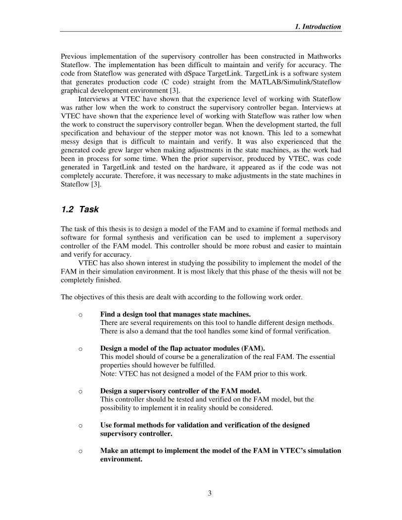
Previous implementation of the supervisory controller has been constructed in Mathworks Stateflow. The implementation has been difficult to maintain and verify for accuracy. The code from Stateflow was generated with dSpace TargetLink. TargetLink is a software system that generates production code (C code) straight from the MATLAB/Simulink/Stateflow graphical development environment [3].

Interviews at VTEC have shown that the experience level of working with Stateflow was rather low when the work to construct the supervisory controller began. Interviews at VTEC have shown that the experience level of working with Stateflow was rather low when the work to construct the supervisory controller began. When the development started, the full specification and behaviour of the stepper motor was not known. This led to a somewhat messy design that is difficult to maintain and verify. It was also experienced that the generated code grew larger when making adjustments in the state machines, as the work had been in process for some time. When the prior supervisor, produced by VTEC, was code generated in TargetLink and tested on the hardware, it appeared as if the code was not completely accurate. Therefore, it was necessary to make adjustments in the state machines in Stateflow [3].

1.2 Task

The task of this thesis is to design a model of the FAM and to examine if formal methods and software for formal synthesis and verification can be used to implement a supervisory controller of the FAM model. This controller should be more robust and easier to maintain and verify for accuracy.

VTEC has also shown interest in studying the possibility to implement the model of the FAM in their simulation environment. It is most likely that this phase of the thesis will not be completely finished. The objectives of this thesis are dealt with according to the following work order.

o Find a design tool that manages state machines. There are several requirements on this tool to handle different design methods. There is also a demand that the tool handles some kind of formal verification.

o Design a model of the flap actuator modules (FAM). This model should of course be a generalization of the real FAM. The essential properties should however be fulfilled. Note: VTEC has not designed a model of the FAM prior to this work.

o Design a supervisory controller of the FAM model. This controller should be tested and verified on the FAM model, but the possibility to implement it in reality should be considered.

o Use formal methods for validation and verification of the designed

supervisory controller.

o Make an attempt to implement the model of the FAM in VTEC’s simulation

environment.

1. Introduction

4

1.3 Delimitation

There are several tools used to design supervisory controllers. This thesis will discuss and examine which tool or tools that are most fit for the task. The model and supervisor will be implemented in only one of these tools.

To implement the model of the FAM in VTEC’s simulation environment is very complex and most likely some adjustments in the simulation design have to be made. An attempt for implementation will be made but due to the time limit of this thesis, it is not certain that this work will be finished. To implement the controller is even more complex and includes code generation. This will not be realized in this thesis.

1.4 Outline

Part one – introduction and methodology

The next chapter in this first part of the thesis will describe the method that has been used when working with this thesis. The theory behind state machines and different design tools will be presented. The thought is to investigate which design tool is the best to solve the tasks presented above.

Part two – implementation in Stateflow

The second part in this thesis is about the implementation in the chosen design tool. The first chapter in this part treats the modeling of the FAM and modeling of the supervisory controller to the FAM. The second and third chapters are about validating and verifying the models. The last chapter in this part treats the attempt to implement our FAM model in VTEC’s simulation environment: Hardware-in-the-loop.

Part three – summing up

The last part of this thesis handles the presentation and analysis of the results. Are the objectives of this thesis reached? In the last chapter there will be a discussion about the results of this thesis. There will also be some suggestions how to continue working with the kind of task this thesis handles.

2. Method

5

2 METHOD

The following chapter will describe the method that has been used when working with this thesis. First of all, some theory about finite state machines and how to design them will be presented. Second there will be information about some of the design tools available on the market.

2.1 Theory

2.1.1 The Finite State Machine

A finite state machine (FSM) is a model of behavior composed of a finite number of states, transitions between those states, and actions. [1]

The FSM is a system that at any time unit occupies a unique state of being, out of a finite set of such states. Man made, non physical systems containing information handling parts, such as manufacturing systems and communication protocols, are profitably modeled as discrete events systems (DES).[1]

transition

event

state

State name

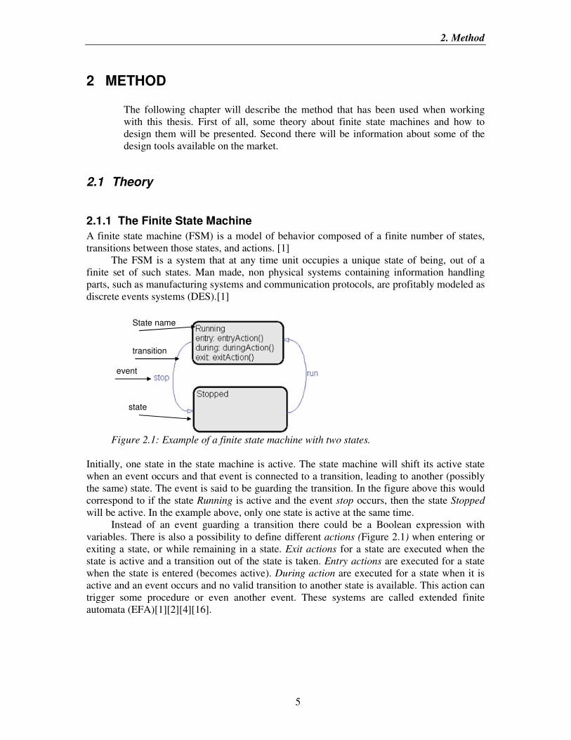
Figure 2.1: Example of a finite state machine with two states.

Initially, one state in the state machine is active. The state machine will shift its active state when an event occurs and that event is connected to a transition, leading to another (possibly the same) state. The event is said to be guarding the transition. In the figure above this would correspond to if the state Running is active and the event stop occurs, then the state Stopped will be active. In the example above, only one state is active at the same time.

Instead of an event guarding a transition there could be a Boolean expression with variables. There is also a possibility to define different actions (Figure 2.1) when entering or exiting a state, or while remaining in a state. Exit actions for a state are executed when the state is active and a transition out of the state is taken. Entry actions are executed for a state when the state is entered (becomes active). During action are executed for a state when it is active and an event occurs and no valid transition to another state is available. This action can trigger some procedure or even another event. These systems are called extended finite automata (EFA)[1][2][4][16].

2. Method

6

2.1.1.1 Mealy and Moore machines

There are generally three types of FSM: Mealy, Moore and classic. Classic statecharts includes both Mealy and Moore semantics. The Moore FSM uses only entry actions, i.e. the output depends only on the state. The advantage of the Moore model is a simplification of the behavior which in turn leads to better code generation. The Mealy FSM uses only input actions, i.e. the output depends on the input and the state. The use of a Mealy FSM often leads to a reduction of the number of states. Often a mixed, classic model is used which in many cases is the easiest solution, compared to using either Mealy or Moore [2].

2.1.1.2 Parallel states

In many systems it is not exclusively one state that is active at the same time. Imagine two machines (e.g. robots) working together in a cell. Each machine could be either running or stopped. Figure 2.2 below illustrates these two machines where machine1 and machine2 has a parallel execution order. The semantic of the system is an AND-operation between machine1 and machine2. The dotted lines indicate that the two states are parallel [4].

Figure 2.2: Example of two parallel FSM

2.1.1.3 Deadlock

It is important to avoid deadlock when designing the state machines. Deadlock refers to a specific condition when two or more processes are each waiting in a circular chain for another to release a resource. This is a state where the system is locked no matter which event occurs. Deadlock is common when several processes, i.e. several FSM, share a mutually exclusive resource, e.g. software. Deadlock may occur if there is dependence between two state machines, e.g. an event in one state machine triggers a transition in the other. This is why it is important to have the execution order in mind when designing machines with parallel states [14].

2.1.1.4 Superstate

In Figure 2.3 there are three states. Since event β takes the system to state B from either A or C, it is tempting to cluster the latter into a new superstate D, depicted in Figure 2.4. The two β arrows are replaced by one. The semantic of D is then the exclusive-or of A and C, i.e. to be in state D one must be either in A or in C, but not in both. D is an abstraction of A and C with the common property that β leads from them to B. One purpose of doing so is to economize the number of arrows, thus making the FSM much easier to survey [12].

2. Method

7

Figure 2.3: FSM with three states[12]

Figure 2.4: FSM with a superstate D[12]

A superstate can itself consist of several other superstates. In this way it is possible to construct a system with hierarchy. In a superstate with several other parallel superstates it is possible with more than one active state at the same time [4].

2.1.1.5 Default transition

Default transitions are primarily used to specify which exclusive (OR) state is to be entered when there is ambiguity among two or more neighboring exclusive (OR) states. They are required when such ambiguity exists. Default transitions have a destination but no source object. For example, default transitions specify which substate of a superstate with exclusive (OR) decomposition the system enters by default, in the absence of any other information such as a history junction (see Figure 2.5). Default transitions are also used to specify that a junction should be entered by default [4].

Figure 2.5: Example of default transition and history junction

2.1.1.6 History Junction

A history junction is used to represent historical decision points in the state machines. The decision points are based on historical data relative to state activity. Placing a history junction in a superstate indicates that historical state activity information is used to determine the next state to become active. The history junction applies only to the level of the hierarchy in which it appears. Not every design tool support history junctions [4].

History junctions override default transition paths in superstates with exclusive (OR) decomposition. In parallel states, a default transition must be present to indicate which of its states is active when the parallel state becomes active [4].

2.1.2 Modeling

A model is an abstraction that tries to capture the characteristics of an object that are important to the user. The real object has an infinite number of attributes, of which the model can only ever capture a finite number. It is therefore crucial that the model captures exactly the relevant characteristics of the real system. It is equally as important that the model

2. Method

8

captures only those aspects that are relevant. Otherwise the model may get too complicated. This implicates that it does not necessarily mean that there exists a single unique model of a given system [16].

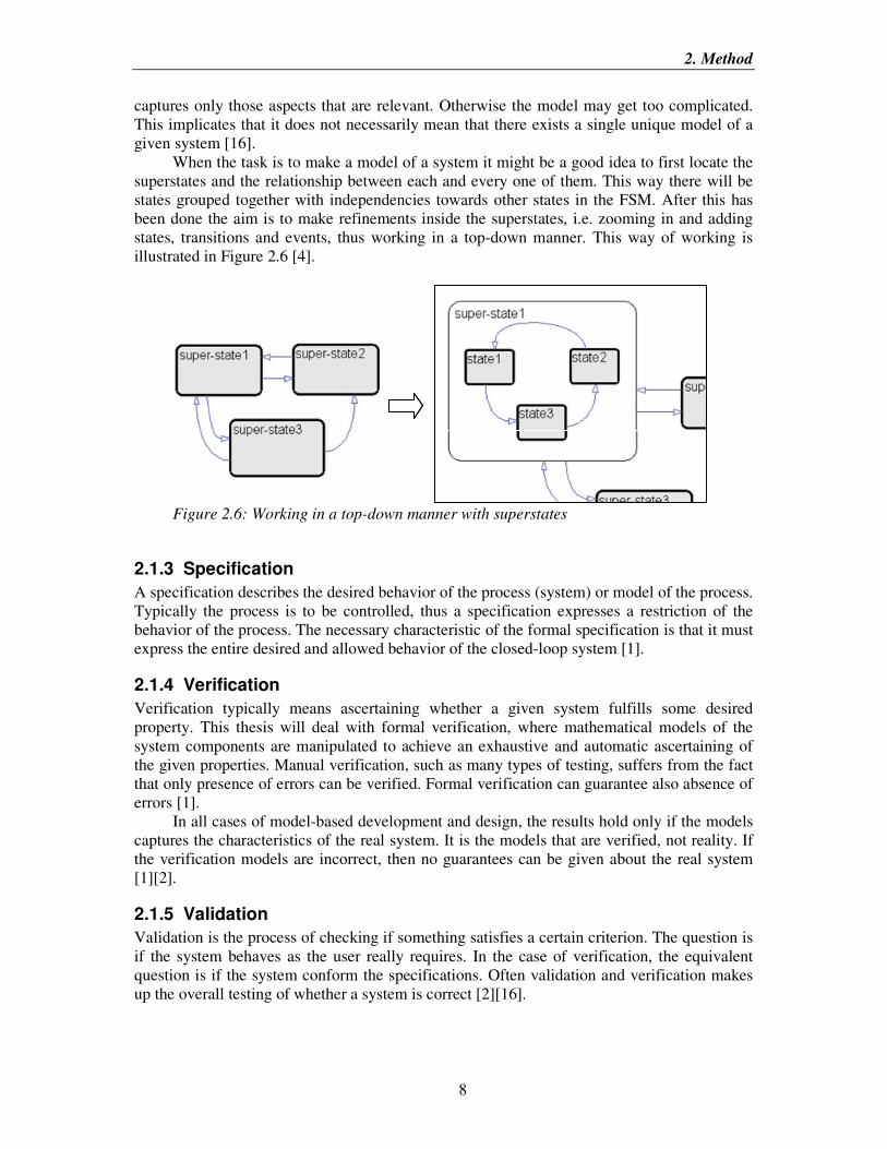
When the task is to make a model of a system it might be a good idea to first locate the superstates and the relationship between each and every one of them. This way there will be states grouped together with independencies towards other states in the FSM. After this has been done the aim is to make refinements inside the superstates, i.e. zooming in and adding states, transitions and events, thus working in a top-down manner. This way of working is illustrated in Figure 2.6 [4].

Figure 2.6: Working in a top-down manner with superstates

2.1.3 Specification

A specification describes the desired behavior of the process (system) or model of the process. Typically the process is to be controlled, thus a specification expresses a restriction of the behavior of the process. The necessary characteristic of the formal specification is that it must express the entire desired and allowed behavior of the closed-loop system [1].

2.1.4 Verification

Verification typically means ascertaining whether a given system fulfills some desired property. This thesis will deal with formal verification, where mathematical models of the system components are manipulated to achieve an exhaustive and automatic ascertaining of the given properties. Manual verification, such as many types of testing, suffers from the fact that only presence of errors can be verified. Formal verification can guarantee also absence of errors [1].

In all cases of model-based development and design, the results hold only if the models captures the characteristics of the real system. It is the models that are verified, not reality. If the verification models are incorrect, then no guarantees can be given about the real system [1][2].

2.1.5 Validation

Validation is the process of checking if something satisfies a certain criterion. The question is if the system behaves as the user really requires. In the case of verification, the equivalent question is if the system conform the specifications. Often validation and verification makes up the overall testing of whether a system is correct [2][16].

2. Method

9

2.1.6 Synthesis

Automatic generation of a controller through some form of algorithm is what we refer to as synthesis. The controller is generated from the process model and the specification. The algorithms to synthesize a controller exist, are well known and easy to implement. Furthermore, the synthesis algorithms have been mathematically proven to always return a correct result. Still there are not many design tools implementing synthesis. However, it is usual to design a controller manually and then verify correctness by formal verification. The adjustments made in the controller, due to results of the verification are a kind of manual synthesis [3][16].

2.2 Design tools

The choice of design tool is first and foremost dictated by availability, but also by the capability of formal verification and design flexibility. A main goal of this thesis work is to investigate and apply a method of verification to ascertain certain properties and control sequences. Therefore it is crucial that the chosen tool has the possibility to perform formal mathematical verification for design correctness and robustness. It is also important that the tool has the modeling potential of designing a model as tight to the specification as possible. For example, basic mathematical functions and variables need to be readily accessible and so on. Seeing that the target is embedded systems, the chosen tool should also be able to generate code, in this case C code, or work with a standalone code generator. This demand is not in main focus, but will be taken into account.

When considering the demands above, we found three software design tools of interest that we decided to look further into. They are described in the following text.

2.2.1 Supremica

Supremica is a tool that helps engineers to develop robust control systems and is developed at Chalmers University. Thus, the authors have been in contact with the software during courses at said university.

Supremica allows the user to model a plant, i.e. the uncontrolled physical system, and to create a specification that expresses the allowed sequences and events of the plant. A synthesis of the two models can then be done. This will result in a supervisory controller that restricts the uncontrolled system such that the closed-loop system fulfills the specifications. This is the main purpose of Supremica [16]. Supremica includes formal verification algorithms to verify controllability and non-blocking properties.

Supremica is also free of charge for education and research and since it is developed mainly at Chalmers, expertise and support on the software is easily available. The documentation is very insufficient and supplementary development takes place abroad.

However, implemented mathematical operators and supported syntaxes are very limited and the documentation covering this area is more or less nonexistent. The use of variable types is also currently limited.

According to Supremica developers, there is a possibility to generate some sort of C code called NQC, Not Quite C. Information regarding this function is not yet available and the function itself is not yet public, but NQC is said to include some of the most basic C commands.

2. Method

10

2.2.2 UPPAAL

UPPAAL is an integrated tool environment for modeling, simulation and verification of real-time systems, developed jointly by Basic Research in Computer Science at Aalborg University in Denmark and the Department of Information Technology at Uppsala University in Sweden. The UPPAAL software is free for non-commercial use. Typical application areas include real-time controllers and communication protocols in particular, those where timing aspects are critical [13].

UPPAAL consists of three main parts: a description language, a simulator and a model-checker. The description language is a non-deterministic guarded command language with simple data types (e.g. bounded integers, arrays, etc.). It serves as a modeling or design language to describe system behavior as networks of automata extended with clock and data variables. The simulator is a validation tool, which enables examination of possible dynamic executions of a system during early design (or modeling) stages. Thus it provides a mean of fault detection prior to verification by the model-checker, which covers the exhaustive dynamic behavior of the system [13].

A downside with UPPAAL is that larger models become hard to overview and that the support for mathematical functions is limited. There is no documentation on UPPAAL’s webpage about any possibility to generate C-code [13].

2.2.3 Stateflow

Stateflow extends Simulink with a design environment for developing state machines and flow charts. Stateflow provides the language elements required to describe complex logic in a natural, readable, and understandable form. It is tightly integrated with MATLAB and Simulink, providing an environment for designing embedded systems that contain control, supervisory, and mode logic.

Stateflow provides language elements, hierarchy, parallelism, and deterministic execution semantics for describing complex logic. It is also possible to define different actions when entering or exiting a state, or while remaining in a state. Exit actions for a state are executed when the state is active and a transition out of the state is taken. Entry actions are executed for a state when the state is entered (becomes active). During actions are executed for a state when no valid transition to another state is available.

Stateflow makes it possible to specify functions graphically using flow diagrams. Embedded MATLAB functions are possible as well as functions in tabular form (truth tables).

The simulation of Stateflow charts logs data to enhance understanding of the system and assist debugging. The debugger itself can be used for setting graphical breakpoints, stepping through charts, and browsing data variables [4].

There are two C code generators available for Stateflow, Target Link and Stateflow Coder. Target Link is developed by dSPACE and Stateflow coder is developed by Mathworks.

2.2.3.1 Design Verifier

Stateflow does not provide the possibility of performing formal verification using mathematical algorithms. However, Stateflow is compatible with the Design Verifier software (also from Mathworks), which generates tests for Stateflow models that satisfy model coverage and user-defined objectives. It also proves model properties and generates examples of violations [5].

Design Verifier does not support every feature in Stateflow. Hence, it is recommended to have this in mind when using Stateflow for modeling purposes. It does not support recursion, calls to MATLAB functions or access to MATLAB workspace variables. Also, it does not support calls to certain C math function supported in Stateflow [5].

2. Method

11

2.3 Results of the design tool study

Of the three design tools that we looked into in the previous chapter, UPPAAL showed to be the least suitable software and our supervisor at Chalmers did not recommend it for our tasks.

Initial modeling attempts were made in both Supremica and Stateflow to decide which software covers most of our modeling and verification demands. In an early stage it was clear that Supremica did not possess the design flexibility necessary for our implementation. It lacked Stateflow’s support for parallelism, mathematical functions and logic as well as history junctions. Also, there is no documentation about the syntax supported in Supremica. The possibility to follow the execution step-by-step and track all data calculations in the graphical debuggers was also a strong reason for choosing Stateflow as the final design tool. Stateflow and Simulink Design Verifier offer a complete suite for flexible modeling and formal verification.

Another strong argument for choosing Stateflow was that VTEC have already been using Simulink and Stateflow in prior work. If our work was to be integrated in VTEC’s software, it would be easier to use Mathworks’ products.

2. Method

12

PART II

IMPLEMENTATION IN STATEFLOW

3. Modeling

13

3 MODELING

The first topic in this chapter will describe how the EATON FAM model was implemented in Stateflow. Secondly, there will be an explanation of how the controller was implemented. The controller has been designed with the purpose to send and receive messages to and from the FAM. Note that both the controller and FAM model use Mealy and Moore semantics, i.e. both are of type classic state machines. The modeling task is too complex to be solved in a manageable way if limited to only Mealy or Moore (2.1.1.1).

3.1 Modeling EATON FAM

As suggested in Chapter 2.1, the first step when modeling the FAM, is to pinpoint the superstates in the system. One of the most important things is to ask which superstates should be parallel (AND) and which should be exclusive (OR).

Figure 3.1: Superstates of the EATON FAM. (dotted line indicates parallelism)

In the FAM there are five distinguished blocks. All of these blocks are working in a parallel execution order. These five blocks can be represented with five superstates in the model. In every moment when running the model, at least one state has to be active in each superstate. The superstates are: communication, move, stall, failure and calibration. These superstates have to be parallel because a change in these states respective is allowed at every time step. In the following, each superstate will be further explained. Some functions and truth tables in the superstates are removed to simplify the figures.

3.1.1 Communication

The communication superstate is where the FAM sends or receives messages to or from the controller. In reality the FAM is continuously listening to the bus for a request or response header (C.2). In the model, these headers are represented by two specific input events instead.

Figure 3.2: Principle of the communication superstate

3. Modeling

14

3.1.2 Move

The move superstate is the state where the move of the shaft is simulated. The shaft is moving when some conditions (Appendix C) in the state machine are fulfilled. The stop transition is triggered from either the stall superstate or the failure superstate.

Figure 3.3: Principle of the move superstate

3.1.3 Stall

The stall superstate handles the stall of the shaft. In the model it is hard to simulate a stall during a movement. This is because a stall depends on several factors. It obviously depends on the distance to the end stop. It also depends on acceleration and speed of the shaft. Stall is simulated with the help of the stallSimulator depicted below. The FAM is stopped, with the stop event in the state stallMode (Figure 3.4).

Figure 3.4: Principle of stall superstate

3.1.4 Failure

The failure superstate contains two states: failureMode and noFailure. When there is failure the FAM is stopped with the stop event. If the Failure Register is equal to anything other than 8, the notCalib flag is set (C.2.2.4). Failure is cleared with the stop_failure event.

Figure 3.5: Principle of the failure superstate

3.1.5 Calibration

The calibration superstate also contains two states: calibrated or notCalibrated.

Figure 3.6: Principle of calibration superstate

3. Modeling

15

3.2 Modeling the controller

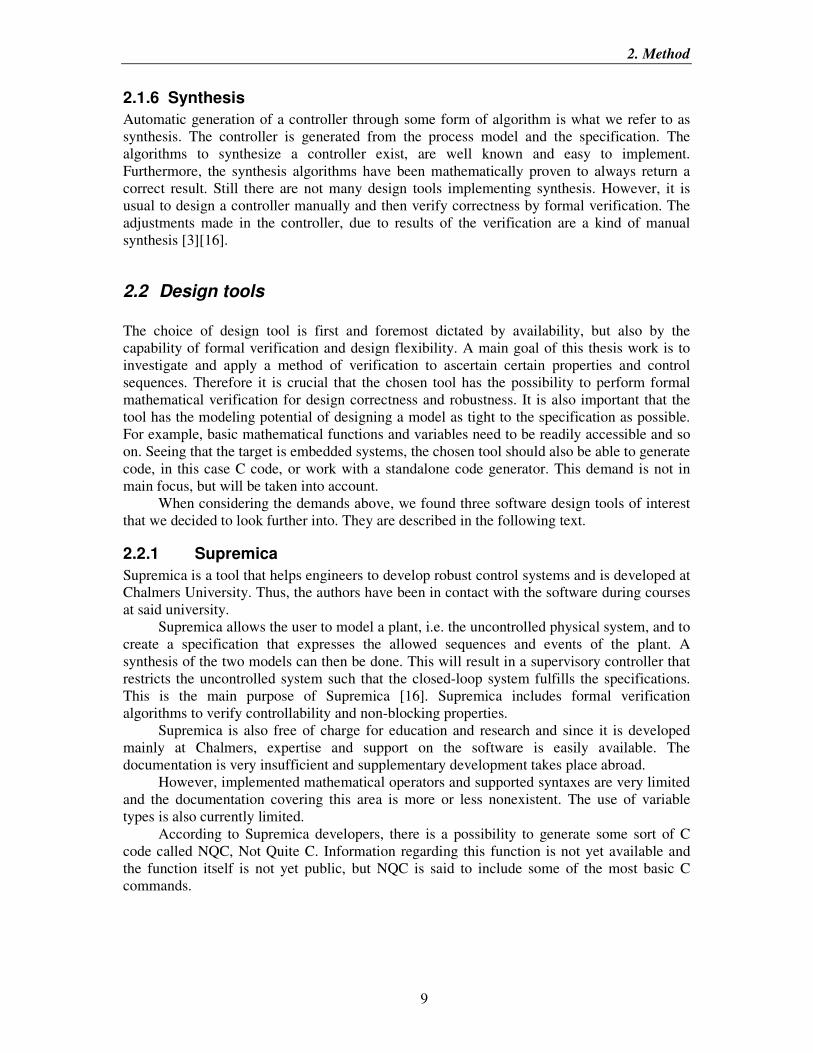
The principle of the design of the controller is very different from the FAM model. It is built based upon hierarchy and history junctions. The design of the controller is depicted in Figure 3.7 and Figure 3.8 below. The two figures are in fact the same controller, but illustrate the principle from two different perspectives. The different blocks represent superstates with different sizes, e.g the requestHandler block includes both the moveHandler and the errorHandler block (Figure 3.7).

The design of this state machine controls one FAM but it is possible to use several instances of this controller in order to control several FAMs. These instances share the same bus. That is why there is a need for a scheduler which controls when each controller is allowed to operate. After a given time interval the scheduler (not illustrated, see Appendix D) sends an event to the controller. This event could mean that the controller should send a request header followed by a request message to the bus. Another event means that the controller should send a response header and then be ready to receive the response message from the FAM. Since these events from the scheduler are generated automatically at a certain time, it is necessary to save historical state activity information by using history junctions (2.1.1.6). To control certain events in the FAM the controller has to send a sequence of different run modes (e.g. see calibration routine D.3.2.1). This is the purpose of the history junctions.

Figure 3.7: Superstates of the Controller. (dotted line indicates parallelism)

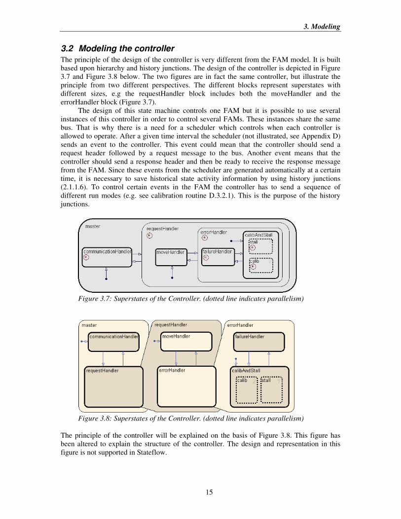
Figure 3.8: Superstates of the Controller. (dotted line indicates parallelism)

The principle of the controller will be explained on the basis of Figure 3.8. This figure has been altered to explain the structure of the controller. The design and representation in this figure is not supported in Stateflow.

3. Modeling

16

3.2.1 Master

The entire controller is included in a single superstate at the top of the state-hierarchy; the master state. The master contains two substates: communicationHandler and requestHandler. The main feature of the controller is to send and receive information from the FAM. This is managed in the communicationHandler. The states in the communicationHandler follow a specific sequence described in D.2. When the controller has received information from the FAM this information has to be interpreted, and that is when the transition is triggered from the communicationHandler to the requestHandler.

Again, at a specific time or timeout, the communicationHandler state is reentered. The information from the FAM has been processed and new control information is to be sent to the FAM. This specific time (timeout) is controlled by the scheduler outside of the controller.

3.2.2 RequestHandler

The requestHandler state processes the information sent from the FAM. The requestHandler contains two substates: moveHandler and errorHandler. When entering the requestHandler superstate for the first time it enters the substate moveHandler, because of its default transition. However, next time the requestHandler state is entered, the history junction (illustrated in Figure 3.7), determines which substate is to be active.

In the moveHandler state, targetPos, swap and runMode is set. There is a transition from the moveHandler to the errorHandler. It is triggered if failure, stall or the need of calibration is present in the FAM. (D.3.1)

3.2.3 ErrorHandler

Stall, failure and calibration are processed in the errorHandler state. There are two substates: failureHandler and calibAndStall. The default transition is assigned to the calibAndStall state. However, a failure is to be prioritized, thus immediately firing the transition from the default state to the failureHandler state if a failure is present.

The failureHandler substate handles the different procedures to reset the different failures. The procedures are further explained in D.3.2.3 When the failures have been reset then the failureHandler substate is exited.

The calibAndStall substate handles stall and calibration of the FAM. This state is also composed of two substates: calibHandler and stallHandler. These two states have a parallel execution order. The reason is because the calibration procedure uses stall detection.

4. Validation

17

4 VALIDATION

This chapter describes how the FAM and the closed system are validated with our MATLAB GUIDE interface. The closed system is our two models, FAM and controller, connected. The controller is controlling the FAM as in the physical system.

4.1 Interface

In order to test sequences and to validate that the FAM and the closed system behave as intended, we constructed a MATLAB GUIDE interface (Figure 4.1). When this application is configured to validate the FAM, it lets the user function as a controller and set all the run modes that are specified in the FAM specification, for detailed information see C.2.1.

You can also invoke stall or failure and set calibration status as well as manually specify the end positions and set the swap flag (C.2.1.1).

When the interface is configured to act upon the closed system, the user can only set a CCM value and invoke errors such as stall, failure, and lost calibration. The run modes are now restricted and set by the controller model itself. One aim of the interface in this mode is to validate correct control sequences when an error is set by the user. Another aim is to check that the FAM reaches its target position correctly.

Figure 4.1: The interface of the FAM, which is used to validate the model

4. Validation

18

4.2 Validating the FAM

The purpose of validating the FAM is to make sure that the specification is implemented correctly in Stateflow. Properties specifically tested were stall detection, swap flag functionality, run modes and also combinations of the previously mentioned features.

4.3 Validating the closed system

As previously stated, the purpose of this validation process is to validate correct control sequence as a result of one or more invoked errors. With the specification as a background, different combinations of errors are set and the behavior of the controller is correlated with the sequences stated in the specification of the controller.

5. Verification

19

5 VERIFICATION

This chapter describes the method and results of formal verification using Design Verifier with Simulink and Stateflow. The FAM and the controller model are verified separately. Attempts were made to verify the closed loop system of the FAM and controller model but the overall complexity of this system made it difficult to use Design Verifier efficiently.

5.1 Design Verifier

One option in Design Verifier is to prove properties. Here, the term property refers to a logical expression of signal values in a model. For example, one can specify that a signal in a model should attain a particular value or range of values during simulation. The Simulink Design Verifier software can then prove whether such properties are valid. The software performs a formal analysis of the model to prove or disprove the specified properties. If the software disproves a property, it provides a counterexample that demonstrates a property violation.

The Simulink Design Verifier software provides two blocks that allow you to specify properties in Simulink models. The Proof Objective block is used to define the values of a signal that the Simulink Design Verifier software will prove. The Proof Assumption block is used to constrain the values of a signal during a proof [5].

5.1.1 Strategies in Stateflow

For complex models, it is often necessary to verify the Stateflow state space directly; for example, to check if two states can be active at the same time. This can be done by assigning a Stateflow outport to an ‘in’-function. An ‘in’-function gives a true answer if the current state is active. Here, state SF_out (Figure 5.1) is parallel and passes state space information to the Simulink workspace and to Design Verifier, e.g. if state s1 is active out1 becomes true .

Figure 5.1: Passing state information to the Simulink workspace.

Another way to achieve this is to use the implemented Design Verifier functions directly in Stateflow. The following syntax invokes these functions in a Stateflow chart:

dv.prove(expr, "{values}")

dv.assume(expr, "{values}")

Design Verifier lacks the ability to directly verify a sequence of events or state entries. This is one downside of Design Verifier, particularly in our case. However, using Simulink and Stateflow blocks and charts, one can construct logic to indirectly verify sequences. This can become somewhat time consuming, and increases the overall complexity of the model. Another problem with Design Verifier occurs when verifying a model with counters. The search process proceeds in a breadth-first manner. All configurations that can be reached in a

5. Verification

20

single time step are investigated before any of the configurations that can be reached in two time steps. Likewise, all configurations that can be reached in two time steps are investigated before any configuration that requires three or more time steps, etc. Thus a counter will expand the search depth with the size of the counter. Therefore, if the design includes large counters, it could be a good idea to choose a small counter value when running Design Verifier analysis [5].

5.1.2 Strategies for Large Models

Proving large and complex models can be very time consuming. This calls for some sort of strategy when setting up the test cases and configuring Design Verifier.

First, use the bounded property proving method. This means searching for property violations to a predefined limit of time steps. If no violations are found within the time span, increase the bounded limit. There is a limit for when the bounded search can be more complex than the unbounded. A recommendation is that if no property violations are found within 50 steps, switch to unbounded property proving. We have found this method of property proving most efficient when proving our models. Often a property violation found quickly in a small bounded limit can take a great deal of time when running the unbounded property proving. However, unbounded property proving is necessary when exhaustively proving the absence of violations [5].

5.2 About the test cases

Generally, it is always better to verify the closed loop system. Parts of the system can be accurate when tested separately, but when the parts are connected different behavior could occur. Hopefully, the closed loop system’s behavior is captured by validating the closed loop system and verifying the FAM and controller separately.

The following test cases exemplify different scenarios that can be verified using Design Verifier. Some of these examples show how Design Verifier can be used to verify that the output variables have correct values. One other important thing to verify is whether some internal states are active at the same time. The reason is that some states are not allowed to be active at the same time. There are of course a lot of other examples of test cases not mentioned below.

The runModes mentioned in the tables below can be found in Table C.2. The states used together with the ‘in’-function are internal states in either the FAM-model or the controller.

5.3 Verifying the FAM model

Can the FAM be in stall-mode and still be running?

Test case 1:

Assertion: runMode={0,1,2,4,6}

Property: (in(stallHandler.stallMode) &&

in(moveHandler.running))==0

(The state stallHandler.stallMode is active when the FAM-model has stalled. The state moveHandler.running is active when the FAM-model is running.)

Results: The property was proven false. This is correct behavior since runMode==FAILURE_RUN is permitted when FAM is in stall mode.

5. Verification

21

Test case 2:

Assertion: runMode={0,1,2,6}

(runMode==5 means FAILURE RUN and is excluded) Property: (in(stallHandler.stallMode) &&

in(moveHandler.running))==0

(The state stallHandler.stallMode is active when the FAM-model has stalled. The state moveHandler.running is active when the FAM-model is running.)

Results: The property was proven true. The FAM will not be able to move when in stallMode and FAILURE_RUN is disabled. This proves that when the FAM is in stall, FAILURE_RUN is the only command that is allowed to move the actuator.

Conclusion:

These two cases prove that the FAM can move in stall mode, but only with the FAILURE_RUN command.

Can the FAM be in failure-mode and still be running?

Test case 1:

Assertion: runMode={0,1,2,4,6}, failureReg={0,1,2,3,4,5,6,7}

Property: (in(failureHandler.failure) &&

in(moveHandler.running))==0

(The state failureHandler.failure is active when failure is present. The state moveHandler.running is active when the FAM-model is running)

Results: The property was proven false. This is correct behavior since run mode FAILURE_RUN is permitted when FAM is in failure.

Test case 2:

Assertion: runMode={0,1,2,6}

(runMode==5 means FAILURE_RUN and is excluded) Property: in(failureHandler.failure) &&

in(moveHandler.running))==0

(The state failureHandler.failure is active when a failure is present. The state moveHandler.running is active when the FAM-model is running)

Results: The property was proven true. The FAM will not be able to move when in failure and FAILURE_RUN is disabled

Conclusion:

These two cases prove that the FAM can move in failure mode, but only with the FAILURE_RUN command.

5. Verification

22

Can the FAM be in notCalib-mode while a communication failure is set? The FAM should not set the notCalib-flag due to a communication failure

Test case:

Assertion: runMode={0,1,2,4,6}, failureReg={0,1,2,3,4,5,6,7}

Property: in(failureHandler.failure) &&

in(calibHandler.notCalib) && failure!=3 (The state failureHandler.failure is active if a failure is present. The state calibHandler.notCalib is active if the FAM requires calibration. Failure==3 means a communication failure.)

Results: The property was proven false. This property is broken by the following sequence of events according to Design Verifier: A failure, other than the communication failure, occurs. This sets the FAM in notCalib-mode. Now, the FAM receives STOP_FAILURE and exits the failure mode. FAM is still in notCalib until the calibration sequence is done. If a communication error would occur before calibration is completed, the above property is broken. Note that this is actually correct behavior for this sequence and not a modeling error.

Can the FAM’s actual position register to be outside the interval [0 4095]?

Test case:

Assertion: targetPos=[0 4095], runMode={0,1,2,4,6}, swap={0,1}

Property: actualPos=[0 4095]

Results: The property proven false. Design Verifier finds actualPos = 4096. Simulation of the generated test harness shows actualPos outside range at time step = 20. After 20 time steps in the graphical debugger an error in our implemented modulus function calculates actualPos to 4096. The error is corrected and the property is proven true.

5. Verification

23

5.4 Verifying the controller

Can the master send NORMAL_RUN if there is a failure in the FAM?

Test case:

Assertion: CCM=[0 1000], failureReg_bit0=[0 1],

input_actualPos=[0 1000], input_notCalib=[0 1],

input_stall=[0 1].

Property: runMode==NORMAL_RUN && getFailure()>0

Results: The property was first proven false. It appeared that if some bit of the failure register was set, there was still a possibility for the controller to send runMode==NORMAL_RUN. The failure bit was acknowledged in the controller but there was not enough time to change the runMode to STOP_FAILURE. The reason was that the controller could not execute enough states to change the run mode before there was a scheduled timeout (3.2). This timeout decides when the controller should send request messages to the FAM. Next time the controller returned to process information from the FAM, the run mode STOP_FAILURE was however set properly. The solution was to increase the number of states that are allowed to execute before there is a timeout from 5 states to 10 states. The results of this property proving were then satisfying. Note: Increasing the timeout to 10 states is not critical considering the real-time scheduling constraints

Is it possible for the Master to handle Stall and failure at the same time?

Test case:

Assertion: CCM=[0 1000], input_stall=[0 1],

failureReg_bit7=[0 7]

Property: The idea was to examine if the controller could handle that stall and failure

were set at the exact same moment, i.e. examine when stall==1 && failureReg_bit7==1.

Results: The property was proven satisfied. If stall was set at the same time as failure, failure was prioritized. When the failure was cleared, the stall procedure was commenced as expected.

5. Verification

24

Are the output variables from the controller within the boundaries?

Test case:

Assertion: CCM=[0 1000], input_stall=[0 1],

input_notCalib=[0 1], failureReg_bit7=[0 7]

Property: output_targetPos=[0 4095], output_runMode=[0 7],

output_swap=[0 1]

Results: The property was proven false. Two important discoveries were made. The first discovery was that the target position could be set in an interval between 0 and 4096. The reason for this was a miscalculation in the modulus function. This was corrected. The second discovery was that many variables in the Stateflow chart were of the type double, thus allowing floating-point values in the design. This was also corrected.

Is it possible for the output variable target position to be outside the boundaries set by the

end positions?

Test case:

Assertion: CCM=[0 1000], input_stall=[0 1], input_notCalib=[0 1], failureReg_bit7=[0 7]

. Property: The property tested was if

targetPos<endPos1 || targetPos>endPos2.

Results: The property was proven false. This property is of course supposed to give a falsified answer. However, important is that the only case when this property is allowed is when the calibration procedure is executed and the objective is to achieve stall near one of the end positions. In that case, the target position is set to 50 steps past the end position.

5.4.1 Defining a sequence property

As previously mentioned, Design Verifier does not have properties for directly verifying a given sequence. A solution to this problem is constructed using a verification subsystem, basically with a Simulink “detect change” block and a very simple state machine. When this subsystem is triggered, it starts to listen to its inport for a specific sequence. If the sequence after the trigger pulse deviates from the desired sequence, the subsystem violates its property block and Design Verifier presents a counter-example. Originally, this sequence logic was created to verify correctness of the runMode variable from the controller, i.e. to verify correct sequence of run modes as a result of an error or stall. It can however be used to verify an arbitrary signal sequence.

.

6. An attempt for implementation in “Hardware-in-the-loop”

25

6 AN ATTEMPT FOR IMPLEMENTATION IN “HARDWARE-IN-THE-LOOP”

Hardware-in-the-loop (HIL) simulation is a technique that is used in the development and testing of complex real-time embedded systems. Software, hardware and a simulated environment are tested in a real-time environment. HIL-simulation provides an efficient platform by adding the complexity of the plant under control to the test platform. The complexity of the plant under control is included in test and development by adding a mathematical representation of all related dynamic systems. These mathematical representations are referred to as the “plant simulation” [15].

VTEC has an HIL-simulation system and uses it among other things for testing of the software. Some of the environment in the car is simulated in Simulink. The idea is to implement the model of the FAM into this simulated environment. This could be helpful in the future when making tests on the HIL-system.

The first problem is to clarify if the FAM model works at all in the HIL-system. The Stateflow FAM model is hence copied into the simulated Simulink environment. Constants are connected to the inputs of the FAM. All the outputs variables except the actualPos are terminated. The system is uploaded into the HIL system. It is possible to survey the actualPos variable in the running system to determine if the FAM model is running. The results are positive and the FAM model is working in the HIL-system. The next thing is to make several instances of the FAM model and see if they are working separately. There was some uncertainty whether the variables in the FAM model are local if the compilation can be run without errors. The result was satisfactory and the variables were found to be local in each FAM model.

The following step is to connect the LIN signals, runMode, swap, targetPos, in the system to the FAM model. After some problems with for example an unconnected cable, we managed to connect the LIN signals to the FAM model and the FAM model worked satisfactory with the HIL system. The output signal actualPos from the model was easy to follow in the control program Control Desktop.

6. An attempt for implementation in “Hardware-in-the-loop”

26

PART III

SUMMING UP

7. Results and analyses

27

7 RESULTS AND ANALYSES This chapter is intended as feedback to the tasks of this thesis work and includes condensed information of our results.

o Find a design tool that manages state machines and design a model of the FAM.

Firstly, using Stateflow for solving this type of modeling problem has been ideal. Even though Supremica may have some advantages concerning verification, it would have been difficult to fully implement the specified behavior for the FAM and the controller.

In an attempt to use Stateflow efficiently from the start, different design patterns were studied to ensure a suitable basic structure for the FAM model. The parallel type structure showed itself ideal for modeling the FAM. Extending or modifying behavior late in the modeling process did not cause any problems.

Ultimately, the objective of the model is to aid the validation and verification of the controller and for that, the FAM model fills its purpose.

o Design a supervisory controller of the FAM model.

A different approach was taken in terms of basic structure for the controller model; an exclusive, non-parallel design pattern was used. By minimizing the number of parallel states and using the hierarchy concept, the sequential behavior of the model was easy to analyze. The history junctions available in Stateflow also proved to be quite useful in this non-parallel method of modeling.

o Use formal methods for validation and verification of the designed supervisory

controller.

The closed loop system, where the controller is actually controlling the FAM model ran basically as expected. Through the constructed MATLAB GUIDE interface different test scenarios were run to validate a correct sequence of the controller. Certain unwanted behavior was found, and corrected. Stateflow’s graphical debugger made it easy to follow the path of execution in the chart and to pin point where the design errors originated.

When it came to Design Verifier and formal verification, the result varied. Design errors that would have been hard to find using only validation and simulation, were found in both the controller and the FAM model. In that sense, formal verification could be applied for verifying models of this complexity and structure. However, the closed loop system grew too complex for Design Verifier and poor results were achieved when performing unbounded exhaustive searches.

o Make an attempt to implement the model of the FAM in the HIL test sytem. The final work included code generation and implementation of the FAM model in the Hardware-In-Loop (HIL) lab. The aim here was to implement five FAM models to aid validation of the existing CCM controller software. This confirmed two things; firstly that these type of models can run without alteration in the HIL and secondly that several instances of the FAM model can run parallel in the HIL environment. Also, our FAM models were directly compatible with the existing CCM software and its control sequences for the actual stepper motors.

8. Conclussion and discussion

28

8 CONCLUSSION AND DISCUSSION

This chapter comments on the results of this thesis. There will be some remarks on how it is working with the design tools Stateflow and Design Verifier. In the end of this chapter we will give some recommendation for further work with these design tools.

8.1 Realization of the thesis

The realization of the thesis has been carried out almost accordingly to the time plan. The first three weeks were used to attain knowledge about the actuators and how the bus protocol is used. Gathering this information included reading the specifications of the FAM and the bus protocol. Not all behavior of the FAM is captured in the specifications and some interviews with employees at VTEC were carried out. This information resulted in the appendices of this thesis.

We have continuously written on the report for this thesis during the work with the different tasks. If this had not been the case the time to finish the different tasks would have been shortened. Two weeks were used for research and for evaluating which design tool that was most suitable for our tasks. The modeling in Stateflow took four weeks and the formal verification also took four weeks to complete. One week was used to implement the FAM model in the HIL lab. The remaining weeks have basically been used for working on the report.

8.2 Evaluation of the thesis result

8.2.1 Designing in Stateflow

The design of the FAM and the Controller models has lead to a rather thorough assessment of Stateflow and its capabilities. Working in Simulink and Stateflow has been quite satisfactory. It is intuitive and easy to understand, especially if you have worked with similar software for modeling DES. Stateflow is flexible and supports a wide spectrum of integrated functions and extensive semantics. In practice, this means that one can almost always tailor the model to a tight fit with the specification and a modeling problem can be solved in many different ways.

The documentation of Simulink and Stateflow are quite exhaustive. The offline help documentation in MATLAB is sufficient when working in Stateflow. There is also a lot of information and examples on the web. We recommend starting with the Stateflow help if the tool is new to the user.

The possibility to graphically debug the design in Stateflow is very appealing. It is easy to observe where a failure occurs in a decision point and consequently easy to know where to correct the design. The only negative aspect of this is that the debugger zooms deeply in to the design and this is quite annoying.

8.2.2 Formal verification – Mathworks’ Simulink Design Verifier

The task to formally verify the system in Design Verifier showed to be the most challenging. One reason is that everything you want to verify must be formulated as a question. For example: If one input signal has a specific value, is it possible to get a forbidden value on the output signal? Each of these questions has to be tested separately. The formal verification tool

8. Conclussion and discussion

29

Design Verifier is quite time consuming. A test could take several hours, and was often set to run overnight.

Sometimes when the test had been running for several hours, the test stopped with the short message: “An error during analysis: Analysis produced error”. There is no possibility for debugging to find where the problem originates. Sometimes the message is “out of memory” instead. The computer capacity should be enough, since the tests were run on an Intel Core 2 Duo T7250 2 GHz with 2 GB memory. When these errors arise the only thing to do is to strip the model until the error disappears.

We used Design Verifier version 1.1 for formal verification but since March 2008, Design Verifier 1.2 has been released. This new version has additional support for Stateflow Embedded MATLAB functions and support for Stateflow Truth Table blocks. The test generation has a new strategy that is optimized for large models and it has also improved data values for detecting errors [5]. This release has not been available for testing for the authors, and maybe some of the mentioned problems have been fixed.

8.3 Recommendation

When using Stateflow in its full extent it is a very powerful tool and we believe that it could be effective when designing systems comparable to ours. A brief look at VTEC’s prior work on the FAM controller in Stateflow shows that Stateflow has not been used as intended. Their controller was designed only with graphical functions. The design is much more difficult to understand and to maintain if changes are to be made.

From the demonstration we had on the department on VTEC, we realize that there is a big interest in Design Verifier. Some of the engineers believe that it could help them in their work when designing in Simulink. It is very helpful in an early stage, when designing Simulink models, to verify correctness. However, Design Verifier does not have a lot of support for continuous blocks in Simulink. There is also no support for S-functions [5]. Design Verifier does however have good support for event driven systems, i.e. Stateflow. Thus, we recommend that Volvo Technology should get a trial license for Design Verifier if the aim is to evaluate an event driven system, specifically Stateflow designs.

We believe that, if working properly in Stateflow and using Design Verifier in an early stage of the design work, time could be saved later on. It is time consuming to test software in the HIL lab since it takes time to build the whole system after changes have been made.

9. Bibliography

30

9 Bibliography

9.1 Literature

[1] Fabian, M. (2005). Discrete Event Systems, Lecture Notes (ESS200),

Chalmers University of Technology. ISSN 1403-266X

[2] Shlaer, S., Mellor, S. (1992). Object Lifecycles – Modeling the World in States. New Jersey: Prentice-Hall inc. ISBN 0-13-629940-7

9.2 Personal Communication

[3] Andersson, Mats Volvo Technology

Fabian, Martin Chalmers university of technology Fridholm Björn Volvo Technology Köllerström, Erik Volvo Technology

9.3 Documentation

[4] Mathworks Stateflow 7.0 documentation.

Directly through Simulink/Stateflow or: <http://www.mathworks.com/access/helpdesk/help/toolbox/stateflow/>(2008-04-15)

[5] Mathworks Design Verifier 1.1 documentation. Directly through Simulink/Design Verifier or: <http://www.mathworks.com/access/helpdesk/help/toolbox/sldv/>(2008-04-15)

9.4 Volvo documentation

[6] Santander, E., Zeraffa, P. (2003). EATON SAM, Actuator and Sensor Division :

BLDC Actuator specification.

[7] Wense, H. (2000). Motorola GmbH: LIN specification package – Revision 1.2.

[8] Volvo Car Corporation (2004). Specification of bus protocol for LIN actuators.

Document id. 31806511

[9] Mårdberg, B. (2000). Volvo Technology AB. Control Design Document for the ECC-S80 project.

Document id. 06200-875.

[10] Mårdberg, B. (xxxx). Volvo Technology AB. An Algorithm for Automobile Climate Control.

SAE971790

9. Bibliography

31

9.5 Internet sources

[11] Volvo Technology AB. About.

<http://www.volvo.com/group/global/en- gb/volvo+group/our+companies/volvotechnologycorporation/> (2008-04-15)

[12] Harel, D. (1987). The Weizmann Institute of Science,Department of Applied Mathematics: Statecharts: A visual formalism for complex systems. <http://www.wisdom.weizmann.ac.il/~dharel/SCANNED.PAPERS/Statecharts.pdf > (2008-04-15)

[13] UPPAAL. About. <http://www.it.uu.se/research/group/darts/papers/texts/UPPAAL-pamphlet.pdf> (2008-04-15)

[14] Computer science: Deadlock and synchronization (2008). I: Encyclopaedia

Britannica Online.

<http://search.eb.com> (2008-04-15)

[15] Gomez, M. (2001). Embedded System Design: Hardware-in-the-Loop Simulation.

<http://www.embedded.com/15201692>(2008-04-15)

[16] Åkesson, K., Fabian, M., Flordal, H. (2007). Supremica in a Nutshell – Draft.

<http://www.supremica.org/media/SupremicaNutshell.pdf>(2008-04-15)

Appendix A

32

A APPENDIX A

SPECIFICATION OF THE COMMUNICATION PROTOCOL

A.1 General

The communication between a Slave Node (SN) and the Master Task follows a protocol, according to the LIN Specification Package, Revision 1.2. This is an extract of that package and includes relevant information when constructing a model of the SN and the master task. [7]

The VCC transmission rate is set to 9600 bit/s ± 2%. The bus consists of a single channel that carries bits. The Physical layer is a single line, wired-AND with pull-up resistors in every node, being supplied from the vehicle power net (VBAT). [7]

The bus can have two logical values: ‘dominant’ and ‘recessive’. The dominant value corresponds to the ground voltage and to the bit value 0. The recessive value corresponds to the battery voltage and the bit value 1.[7]

A.2 Message Transfer

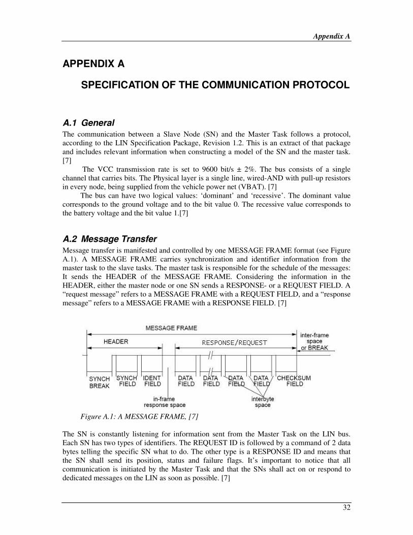
Message transfer is manifested and controlled by one MESSAGE FRAME format (see Figure A.1). A MESSAGE FRAME carries synchronization and identifier information from the master task to the slave tasks. The master task is responsible for the schedule of the messages: It sends the HEADER of the MESSAGE FRAME. Considering the information in the HEADER, either the master node or one SN sends a RESPONSE- or a REQUEST FIELD. A “request message” refers to a MESSAGE FRAME with a REQUEST FIELD, and a “response message” refers to a MESSAGE FRAME with a RESPONSE FIELD. [7]

Figure A.1: A MESSAGE FRAME, [7]

The SN is constantly listening for information sent from the Master Task on the LIN bus. Each SN has two types of identifiers. The REQUEST ID is followed by a command of 2 data bytes telling the specific SN what to do. The other type is a RESPONSE ID and means that the SN shall send its position, status and failure flags. It’s important to notice that all communication is initiated by the Master Task and that the SNs shall act on or respond to dedicated messages on the LIN as soon as possible. [7]

Appendix A

33

A.2.1 MESSAGE FRAME

A.2.1.1 BYTE fields

The BYTE FIELD format (Figure A.2) has a lenght of ten BIT TIMES. The START BIT marks the begin of the BYTE FIELD and is dominant. It is followed by eight DATA BITS with the LSB first. The STOP BIT marks the end of the BYTE FIELD and is recessive. [7]

Figure A.2: BYTE FIELD, [7]

A.2.1.2 Header fields

The Header contains three fields: SYNCH BREAK, SYNCH FIELD and IDENT FIELD.

SYNCH BREAK

Every message header is initiated with a SYNCH BREAK to clearly identify the beginning of a new message; this part is the dominant bus value with a minimum duration of TSYNBRK. Next part of the SYNCH BREAK is a recessive synchronization delimiter with a minimum duration of at least TSYNDEL. This enables the slave to recognize the start bit of the following SYNCH FIELD. [7]

Maximum time for TSYNBRK and TSYNDEL are not stated, but must fit into the message header time budget of THEADER_MAX. Minimum time for TSYNBRK and TSYNDEL is 13 Tbit respectively 1 Tbit.[7]

Figure A.3: SYNCH BREAK

SYNCH FIELD

The synch field gives information for the slave clock synchronization. The field itself is the pattern of 0x55, which gives five falling edges within 8 bit time distance. The field is initiated with a start bit and ends with a stop bit. It is recommended to measure the time between the falling edges of both, the start bit and bit 7, and to divide the obtained value by 8. This value is the time unit Tbit.[7]

Appendix A

34

Figure A.4: SYNCH FIELD [7]

IDENT FIELD

The last part of the header is the identifier field which specifies content, destination and length of a message. [7]

Figure A.5: IDENT FIELD [7]

ID0…ID3 is the ID-bits and states message type and receiver node. ID4, ID5 are the length control bits defining the length of the message, i.e. number of data bytes. Finally the parity check bits set below: [7]

)(54311

)(42100

parityoddIDIDIDIDP

parityevenIDIDIDIDP

⊕⊕⊕=

⊕⊕⊕= Equation A.1[7]

This way no pattern with all bits recessive or dominant will be possible.[7]

A.2.1.3 RESPONSE/REQUEST field

The Response/Request field contains two, four or eight DATA FIELDs (quantity specified in the IDENT FIELD). The last field in the RESPONSE/REQUEST field is the CHECKSUM FIELD) [7]

DATA FIELD

The DATA FIELD consists of a eight bits of data. The LSB is transmitted first (Figure A.6). If the MESSAGE FRAME contains a RESPONSE field, the master task expect information from the SN. And if the MESSAGE FRAME includes a REQUEST field, the SN expect information from the master task. [7]

Appendix A

35

Figure A.6: DATA FIELD [7]

CHECKSUM FIELD

The purpose of the CHECKSUM FIELD is to detect errors in the message. When all the numbers in the RESPONSE/REQUEST field is added, the sum should be ‘0xFF’. The sum is calculated by ‘ADD with Carry ‘ where the carry bit of each addition is added to the LSB of its resulting sum. The CHECKSUM FIELD is designed specificly for this purpose. [7]

A.2.2 Length of message frame

The BYTE-FIELDS within a MESSAGE FRAME are seperated by inter-byte-spaces and in-fram responce space. The length for these variables are not specified, only the total length of a MESSAGE FRAME is limited. The minimum Frame length TFRAME_MIN is the minimum time needed to transmit a complete frame (length of interbyte-spaces and in-frame response space = 0). The maximum Frame length TFRAME _MAX is the maximum time allowed for the transmission of the frame. The values are given in Table A.1. They are dependent on the number of Data Byte Fields NDATA and do not include system inherent signal delays. [7]

Table A.1: Timing of a Message Frame[7]

TIME NAME Time [Tbit]

Minimum Length of Message Frame TFRAME_MIN 10 * NDATA + 44

Minimum Length of Header THEADER_MIN 34

Maximum Length of Header THEADER_MAX (THEADER_MIN +1) * 1.4

Maximum Length of Message Frame TFRAME_MAX (TFRAME_MIN +1) * 1.4

Bus Idle Time-Out TTIME_OUT 25,000

Appendix B

36

B APPENDIX B

VARIABLES Table B.2 and B.3 are lists of the input-, output and internal variables mentioned in Appendix . The variables are used when designing the FAM model and the controller in Stateflow. The variables are also illustrated in D.2.

Table B.2: Variables used in the FAM

Type

Name Length Description

Input

(LIN):

runMode 3-bits The master requests the slave to execute this command or run mode.

targetPos 12-bits The desired position of the slave node swap 1-bit See D.3.1.1

Internal

variables:

endPos1 12-bits The first end stop

endPos2 12-bits The second end stop Range 12-bits endPos2-endPos1

Output

(LIN)

Actuator status: notCalib

stall

dir

run

1-bit 1-bit 1-bit 1-bit

Describes which state the particular slave node is in.

actualPos 12-bits Actual position of the slave node Last_min_torque 8-bits The minimum torque during a

movement. This is not used when modelling the FAM or controller.

Last_max_torque 8-bits The maximum torque during a movement. This is not used when modelling the FAM or controller.

failureReg_bit0

-

failureReg_bit7

8-bits If the slave node recognize a failure the register bits are set.

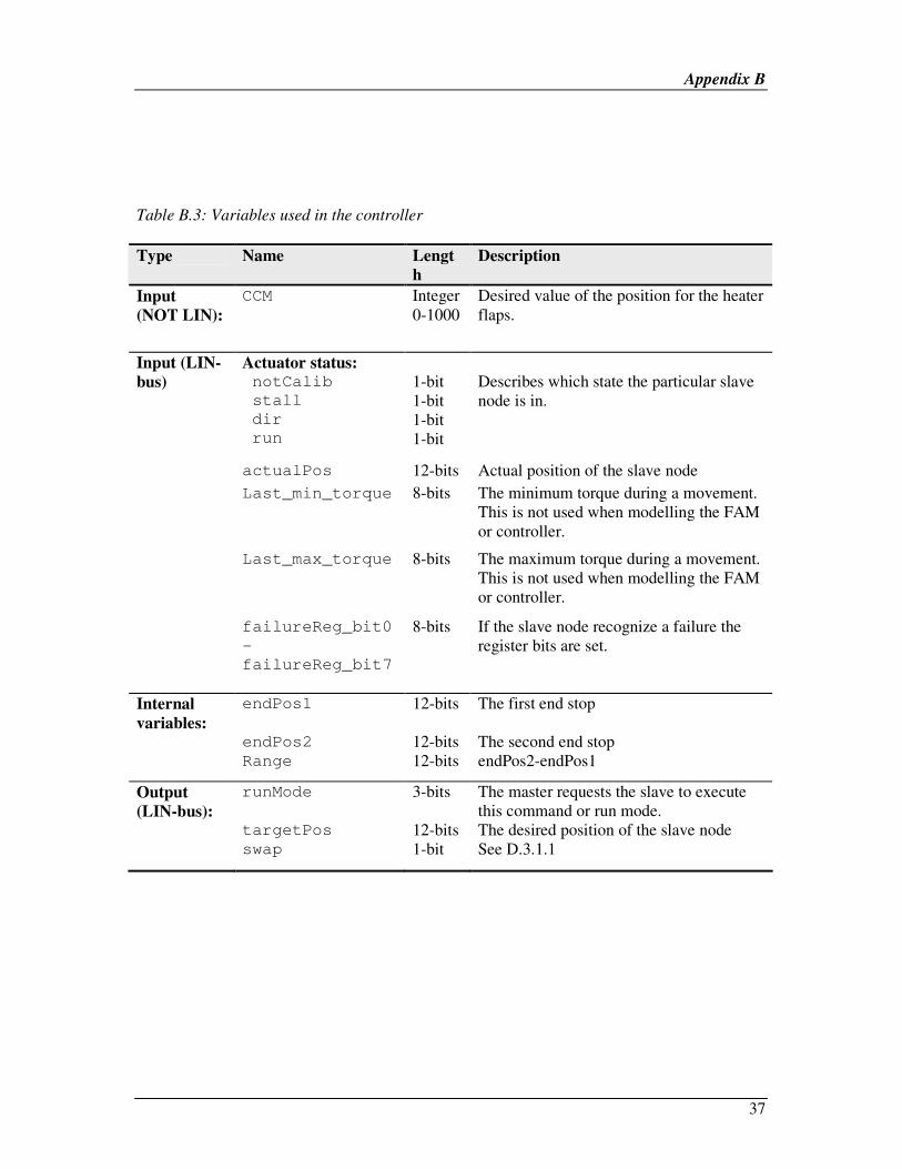
Appendix B

37

Table B.3: Variables used in the controller

Type

Name Lengt

h

Description

Input

(NOT LIN):

CCM Integer 0-1000

Desired value of the position for the heater flaps.

Input (LIN-

bus)

Actuator status: notCalib

stall

dir

run

1-bit 1-bit 1-bit 1-bit

Describes which state the particular slave node is in.

actualPos 12-bits Actual position of the slave node Last_min_torque 8-bits The minimum torque during a movement.

This is not used when modelling the FAM or controller.

Last_max_torque 8-bits The maximum torque during a movement. This is not used when modelling the FAM or controller.

failureReg_bit0

-

failureReg_bit7

8-bits If the slave node recognize a failure the register bits are set.

Internal

variables:

endPos1 12-bits The first end stop

endPos2 12-bits The second end stop Range 12-bits endPos2-endPos1

Output

(LIN-bus):

runMode 3-bits The master requests the slave to execute this command or run mode.

targetPos 12-bits The desired position of the slave node swap 1-bit See D.3.1.1

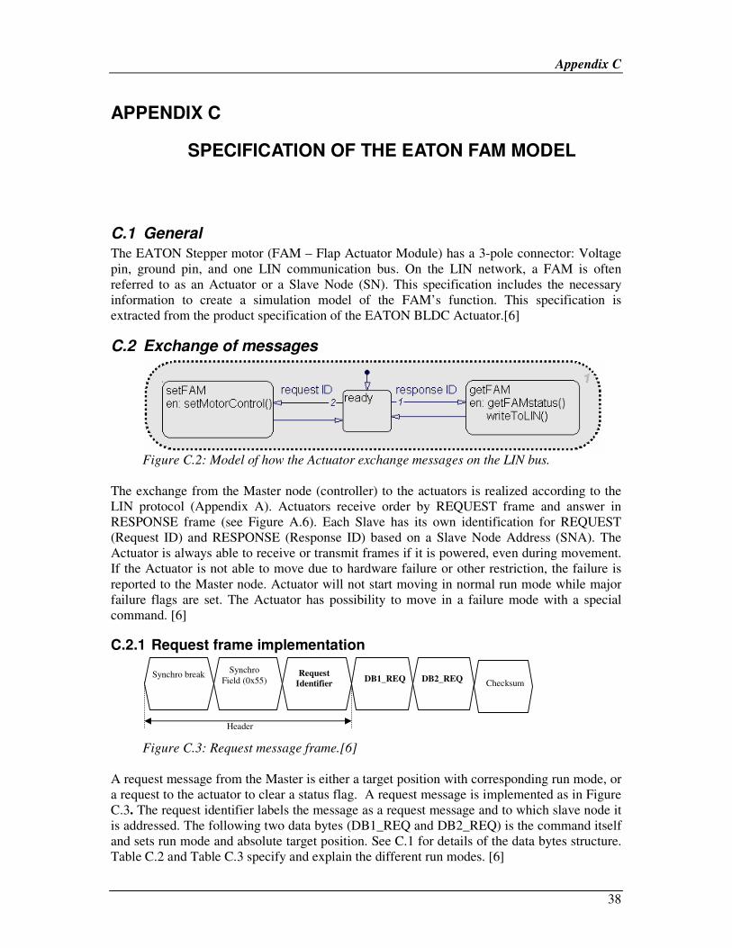
Appendix C

38

C APPENDIX C

SPECIFICATION OF THE EATON FAM MODEL

C.1 General

The EATON Stepper motor (FAM – Flap Actuator Module) has a 3-pole connector: Voltage pin, ground pin, and one LIN communication bus. On the LIN network, a FAM is often referred to as an Actuator or a Slave Node (SN). This specification includes the necessary information to create a simulation model of the FAM’s function. This specification is extracted from the product specification of the EATON BLDC Actuator.[6]

C.2 Exchange of messages

Figure C.2: Model of how the Actuator exchange messages on the LIN bus.

The exchange from the Master node (controller) to the actuators is realized according to the LIN protocol (Appendix A). Actuators receive order by REQUEST frame and answer in RESPONSE frame (see Figure A.6). Each Slave has its own identification for REQUEST (Request ID) and RESPONSE (Response ID) based on a Slave Node Address (SNA). The Actuator is always able to receive or transmit frames if it is powered, even during movement. If the Actuator is not able to move due to hardware failure or other restriction, the failure is reported to the Master node. Actuator will not start moving in normal run mode while major failure flags are set. The Actuator has possibility to move in a failure mode with a special command. [6]

C.2.1 Request frame implementation

Figure C.3: Request message frame.[6]

A request message from the Master is either a target position with corresponding run mode, or a request to the actuator to clear a status flag. A request message is implemented as in Figure C.3. The request identifier labels the message as a request message and to which slave node it is addressed. The following two data bytes (DB1_REQ and DB2_REQ) is the command itself and sets run mode and absolute target position. See C.1 for details of the data bytes structure. Table C.2 and Table C.3 specify and explain the different run modes. [6]

Header

Request Identifier

Synchro break Synchro Field (0x55) DB1_REQ Checksum DB2_REQ

Appendix C

39

Note that if the actuator experiences hardware failure, stall or other restriction, the failure flag is set and reported to the Master. The actuator cannot move in normal run mode until failure flag is acknowledged and cleared by the Master. However, the actuator can move in failure state with a special run command. For information on the checksum implementation, see A.2.1.3. [6]

Table C.1: Bit configuration of DB1_REQ and DB2_REQ.[6]

Table C.2: Run mode specification. [6]

Data Byte 1

RUN mode

bit 7 bit 6 Bit 5 Name Description

0 0 0 STOP_STALL Stop actuator and clear stall flag 0 0 1 STOP_FAILURE Stop actuator and clear failure flags

0 1 0 NORMAL_RUN Actuator moves to target position in a closed loop. Depending on requested movement angle, the actuator uses high or low speed.

0 1 1 NORMAL RUN FIXED LOW

Actuator moves (speed fixed) to target position in a closed loop.

1 0 0 FAILURE RUN Actuator moves to target without feedback

1 0 1 NORMAL RUN LOW

Actuator moves in low speed mode to target position in a closed loop.

1 1 0 CLEAR_NOT-CALIB

Clear notCalib flag

1 1 1 NORMAL RUN HIGH

Actuator moves in High speed mode to target position in a closed loop

Table C.3: Explanation of the different RUN modes. [6]

RUN MODE STOP_STALL(b000)

Actuator is

running

Stops the actuator. Stall flag is cleared when the motor has stopped completely. Note: If stall is detected and not acknowledge by LIN Master, the motor can

move only in failure mode; normal run mode is inhibited until stall flag is

cleared.

Actuator is

stopped

Actuator Stall status =1 :This command acknowledge the stall detection Actuator Stall status =0 : No action

DB1_REQ

Bit 7 Bit 6 Bit 5 Bit 4 Bit 3 Bit 2 Bit 1 Bit 0

RUN MODE SWAP FLAG TARGET POS (MSB)

DB2_REQ

Bit 7 Bit 6 Bit 5 Bit 4 Bit 3 Bit 2 Bit 1 Bit 0

TARGET POS (LSB)

Appendix C

40

RUN MODE STOP_FAILURE(b001)

Actuator is

running

Stops the actuator. Failure flag is cleared when the motor has stopped completely. Note: Except communication failure, if a failure is detected the motor can

move only in failure mode; normal run mode is inhibited until failure flag is

cleared

Actuator is

stopped

This command acknowledge the failure detection, if the reason of failure has disappeared (example over-voltage detected: this failure can’t be cleared until voltage has decreased under over-voltage detection) If no failure was detected : No action

RUN MODE NORMAL RUN (b010)

Actuator is

running

If the target position has changed, the actuator will start moving towards the new target. If the target is the same as it is serving : No action

Actuator is

stopped

LIN master requests the actuator to move in normal mode to target postion in a closed loop by a feedback hall effect sensor. The speed is controlled but not fixed. Depending on requested movement angle the actuator uses high or low speed: The low speed (low noise) is requested for movements shorter then 44 ± 0.17° and high speed for longer. In normal run mode (high or low speed) the stall detection at constant torque functionality is enabled (48Ncm ± 5Ncm). - High speed : 7.8rpm ±0.5rpm @0N.cm @ 13.5V - Low noise : speed not fixed The motor can not acknowledge this request if the motor is in failure (except communication failure) or if stall detection is not acknowledged by the Master.

RUN MODE NORMAL RUN FIXED LOW (b011)

Actuator is

running

If the target position has changed, the actuator will start moving towards the new target. If the target is the same as it is serving : No action

Actuator is

stopped

LIN Master requests the actuator to move in stepper mode to target position in a closed loop by a feedback hall effect sensor. The speed is fixed (210steps/s). Stall detection functionality is enabled but not accurate (not at constant torque), the actuator may loose step (EPM failure) when it reaches a stall. The motor can not acknowledge this request if the motor is in failure (except communication failure) or if stall detection is not acknowledge by the Master

RUN MODE FAILURE RUN (b100)

Actuator is

running

If the target position has changed, the actuator will start moving towards the new target. If the target is the same as it is serving : No action

Actuator is

stopped

Request to the actuator to moves in Failure mode to target position without feedback (stepper mode). In this mode the speed is fixed (210steps/s) Stall detection functionality is disabled. Note: This mode could be used when the motor is in failure, which can not be

cleared. No inhibition to run in this mode.

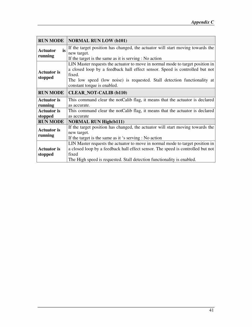
Appendix C

41

RUN MODE NORMAL RUN LOW (b101)

Actuator is

running

If the target position has changed, the actuator will start moving towards the new target. If the target is the same as it is serving : No action

Actuator is

stopped

LIN Master requests the actuator to move in normal mode to target position in a closed loop by a feedback hall effect sensor. Speed is controlled but not fixed. The low speed (low noise) is requested. Stall detection functionality at constant torque is enabled.

RUN MODE CLEAR_NOT-CALIB (b110)

Actuator is

running

This command clear the notCalib flag, it means that the actuator is declared as accurate.

Actuator is

stopped

This command clear the notCalib flag, it means that the actuator is declared as accurate

RUN MODE NORMAL RUN High(b111)

Actuator is

running

If the target position has changed, the actuator will start moving towards the new target. If the target is the same as it ‘s serving : No action

Actuator is

stopped

LIN Master requests the actuator to move in normal mode to target position in a closed loop by a feedback hall effect sensor. The speed is controlled but not fixed The High speed is requested. Stall detection functionality is enabled.

Appendix C

42

C.2.1.1 Position calculus and SWAP FLAG

The actuator uses a 12-bit position representation of the output shaft, which means 0…4095 addressable positions. If the swap flag is not toggled, the need of movement is calculated in the actuator motor control according to Table C.4 example case 1.

When the actuator receives a REQUEST message with the swap flag set, it means that the target position is shifted by the master task. The actuator motor control calculates an shifted actual position.. The actuator is fed these shifted positions and coordinates the move that now has been shifted into an addressable range. For more information of the swap flag see Appendix D.3.1.1. [6]

Table C.4: Position calculation. [6]

Ex.

case

ACTUAL

POS

Register

SWAP

flag

SHIFTED

ACTUAL POS

GOAL

POS

Register

MOTOR CONTROL

(need of movement)

1 actual

Pos 0 actualPos

Target

Pos targetPos–actualPos

2 actual

Pos 1

actualPos

XOR 0x800

Target

Pos

XOR 0x800

(targetPos XOR 0x800) – (actualPos XOR 0x800)

C.2.2 Response frame implementation

When the LIN master sends a response message header on the bus, corresponding slave will as soon as possible reply with its response data (Figure C.4). The response includes actuator information stated in Table C.5 with further explanation and implementation in Table C.6 and Table C.7. [6]

response

IdentifierSynchro

break

Synchro Field (0x55)

DB1_RES ChecksumDB2_RES DB3_RES DB4_RES DB5_RES

Header

Response field

response

IdentifierSynchro

break

Synchro Field (0x55)

response

IdentifierSynchro

break

Synchro Field (0x55)

DB1_RES ChecksumDB2_RES DB3_RES DB4_RES DB5_RESDB1_RES ChecksumDB2_RES DB3_RES DB4_RES DB5_RES

Header

Response field

Figure C.4: Response message frame and actuator response. [6]

Appendix C

43

Table C.5 : Bit configuration of DB1_RES…DB5_RES. [6]

DB1_RES

Bit 7 Bit 6 Bit 5 Bit 4 Bit 3 Bit 2 Bit 1 Bit 0 Actuator STATUS ACTUAL POS (MSB)

DB2_RES

Bit 7 Bit 6 Bit 5 Bit 4 Bit 3 Bit 2 Bit 1 Bit 0 ACTUAL POS (LSB)

DB3_RES

Bit 7 Bit 6 Bit 5 Bit 4 Bit 3 Bit 2 Bit 1 Bit 0 Last Min Torque

DB4_RES

Bit 7 Bit 6 Bit 5 Bit 4 Bit 3 Bit 2 Bit 1 Bit 0 Last Max Torque

DB5_RES

Bit 7 Bit 6 Bit 5 Bit 4 Bit 3 Bit 2 Bit 1 Bit 0 Failure Register

C.2.2.1 Implementation of the actuator status (DB1_RES bit 7...bit 4)

Table C.6: Implementation of the actuator status flags. [6]

Data Byte 1

Actuator Status

Bit 7

NOT-

CALIB

Bit 6

STALL

Bit 5

DIR

Bit 4

RUN

Description in normal condition

0 - - - actualPos is accurate 1 - - - actualPos is not accurate. Calibration is required - 0 - - Actuator has reached the goal position without stall - 1 - - Actuator has stalled - - 0 - Last or actual movement is incremental - - 1 - Last or actual movement is decremental - - - 0 Actuator is stopped - - - 1 Actuator is running

Table C.7: Activation and reset of Status flags. [6]

FLAG NOT-CALIB (bit #7)

Actuator behavior

Normal behavior

Activation condition

Flag is set when actuator has detected conditions which may have corrupted its actual position. This condition are failure, or when actuator detects an end stop after a travel length move shorter than 3.4°C (20 pos =40 steps).

Reset condition Flag is cleared when the master requests CLEAR_NOT-CALIB.

Appendix C

44

FLAG STALL (bit #6)

Actuator behavior

Actuator is blocked and no NORMAL_RUN until stall flag is acknowledged from the master. When the stall condition is detected the actuator stops and sets stall flag.

Activation condition

Flag is set when the torque reach the defined stall limit.

Reset condition Flag is cleared when the master request the STOP_STALL.

FLAG DIR (bit #5)

Actuator behavior

Presents the present or last movement direction.

Activation condition

Flag is set with decrement move direction.

Reset condition Flag is cleared with incremental move direction.

FLAG RUN (bit #4)

Actuator behavior

Actuator is Running.

Activation condition

Flag is set while the actuator is running.

Reset condition Flag is cleared when actuator is stopped.

C.2.2.2 Implementation of the Last Min Torque (DB3_RES)

The Last Min Torque is the measured information torque during the movement. The torque values are relative and without unit. This value is not implemented in the FAM model. [6]

The torque is measured continuously between two consecutive response frames. When the LIN actuator is stopped due to stall condition it shall use the « torque »value measured when the stall was detected. The value is set to 0xFF when the stall flag is cleared. [6]

C.2.2.3 Implementation of the Last Max Torque (DB4_RES)

The Last Max Torque is the measured information torque (without unit) during the movement. The torque values are relative and without unit. This value is not implemented in the FAM model. [6]

The torque is measured continuously between two consecutive response frames. When the LIN actuator is stopped due to stall condition it shall use the « torque » value measured when the stall was detected. The value is set to 0xFF when the stall flag is cleared (and motor is stopped). [6]

C.2.2.4 Implementation of the failure flags (DB5_RES)

When a failure is set, except communication failure (bit3), the actuator is kept in stop mode until failure flag is cleared from LIN master. Only run in failure mode command allows actuator to move. The notCalib flag is set when each failure, except Communication failure (bit #3), is triggered. [6]

Appendix C

45

Table C.8 describes the failure register (DB5_RES) and explanation, how the flags are set and how to reset the flags, is found in Table C.9.

Table C.8 Failure register. [6]

Data Byte 5

Failure Register

bit 7 bit 6 bit 5 Bit 4 Bit 3 Bit 2 Bit1 Bit0

Hall sensor supply current limitation

Default position restore (0x800)

Extreme position maintain-able (EPM)

Over voltage or over temperature

Communic-ation failure

Feedback failure

Coil circuit failure or coil driver failure

Calibration lost during movement when power failed

Table C.9: Activation and reset of failure flags. [6]

Flag Bit #7

Flag Name Hall Sensor supply current Limitation (HSL)

Flag Activation

condition Flag is set when the hall sensor output exceed the current limitation.

Flag Reset condition Flag is cleared when current has decreased below the limit and the master requests the STOP_FAILURE mode.

Actuator behavior

When failure flag is set the actuator is only able to run in FAILURE_RUN mode. In FAILURE_RUN mode the hall sensor feedback is disabled. No stall detection is possible. The actuator will loose positions if it was running when this failure occurred.

Flag Bit #6

Flag Name Default position restore (0x800) (DPR)

Flag Activation

condition

Flag is set after actuator is reset and default position has to be restored in actuator memory because normal position save failed

Flag Reset condition Flag is cleared when the master requests the STOP_FAILURE mode.

Actuator behavior After a reset the actuator has not been able to restore a position from the Memory bank and will retrieve the position 0x800. Actuator remains stopped until failure flag is cleared.

Flag Bit #5

Flag Name Extreme position maintainable (EPM)

Flag Activation

condition

Flag is set when actuator is stopped and is unable to keep its position. External force on the flap may trigger this event. This failure can occur, if CCM request to reach stall detection while the actuator is already in a grey zone.

Flag Reset condition Flag is cleared when the master requests the STOP_FAILURE mode.

Actuator behavior

If the external, not controlled, force or the end stop pushing force is larger then the holding torque, the actuator is not able to keep its position. Actuator remains stopped until failure flag is cleared.

Appendix C

46

Flag Bit #4

Flag Name Over voltage or over temperature (OTF)

Flag Activation

condition

Flag is set when thermal disjunction detected by the hardware (typical 140°C) or if over voltage above +18V is detected

Flag Reset condition

The thermal disjunction has to decrease to at least 20°C and the voltage has to decrease below +16V until the failure flag can be cleared. Flag is cleared when the master requests the STOP_FAILURE mode.

Actuator behavior

Coil is switched off when thermal disjunction detected or over voltage is detected. The actuator stops as soon as possible, dependent on rotor speed when the coil is switched off. Actuator remains stopped until failure flag is cleared. (It can move only in FAILURE mode) The actuator will lose positions if it was running when failure occurred.

Flag Bit #3

Flag Name Communication Failure (COF)

Flag Activation

condition

Flag is set when Communication failure occur.

Flag Reset condition Flag is cleared when the master requests the STOP_FAILURE mode.

Actuator behavior

When a problem of a LIN frame request is detected the COF flag is set. The Received message will be scrapped. The COF fag will not affect any other functionality (still able to run actuator).The problems with a LIN frame which will cause the COF flag to be set are: bit frame error synchronization oscillator error synchronization byte error parity error time out error over run error If the header is cancelled or dropped by the master task, the actuator keeps the latest OK message.

Flag Bit #2

Flag Name Feedback failure (FBF)

Flag Activation

condition

Flag is set when the synchronization between the hall sensor feedback and the coil commutation is missed.

Flag Reset condition Flag is cleared when the master requests the STOP_FAILURE mode.

Actuator behavior

When the synchronization between the hall sensor feedback and the coil commutation fails the actuator stops. Actuator remains stopped until failure flag is cleared. It may be caused if the "Hall sensors supply current limitation" appears. While failure flag is active the actuator can only run in FAILURE_RUN mode.

Appendix C

47

Flag Bit #1

Flag Name Coil circuit failure or coil driver failure (CCF)

Flag Activation

condition

Flag is set when actuator is stopped and an open coil circuit appears. On external move, the rotation of the magnet generate a back electromagnetic voltage in the motor coil up to 45 V. This failure will be diagnostic first as an EPM but also as a coil failure.

Flag Reset condition Flag is cleared when the master requests the STOP_FAILURE mode and the failure has disappeared.

Actuator behavior

Unknown behavior when coil circuit gets open when the actuator is running. Rotor can continue to rotate, stop or turn in reverse direction. Actuator is kept in stop until failure flag is cleared. While failure flag is active the actuator can only run in FAILURE_RUN mode.

Flag Bit #0

Flag Name Calibration lost during movement when Power Failed (CPF)

Flag Activation

condition

Flag is set after actuator reset and if the actuator has detected calibration lost during movement when power failed.

Flag Reset condition Flag CPF is cleared when the master requests the STOP_FAILURE mode.

Actuator behavior

The CPF will occur if power is lost (Ubat < 8V) when actuator is running. The Actuator will then brake the rotor for 10 ms before position is saved in EEPROM. The flag will also be stored in EEPROM that indicate a CPF. Actuator remains stopped until failure flag is cleared.

Appendix D

48

D APPENDIX D

SPECIFICATION OF THE MASTER TASK

D.1 General

The master task is the controller of the Slave nodes. The master task communicates with the different slave nodes in a particular sequence, according to a scheduled loop. The principle is illustrated in Figure D.1; the master task sends a message to all slave nodes, respectively. When all the slave nodes have been addressed, the master task requires the slave nodes to respond with their current status. After this the routine starts over from the top again. [6]

header Request field Addressed to slave 1

header Request field Addressed to slave n

header

Response field

Addressed to slave 1

header

Response field

Addressed to slave n

Response from slave 1

Response from slave n

header Request field Addressed to slave 1

header Addressed to slave n

header

Response field

Addressed to slave 1

header

Response field

Addressed to slave n

Response from slave 1

Response from slave n Figure D.1: Schedule for the communication between master and slaves

The master task checks the consistency of a message being initiated by the master task and being received by its own slave task. In case of inconsistency the master task can change the message schedule.

D.2 Communication

The Master task communicates with the slave node using the LIN protocol (see Appendix A). The master task initiates the message transfer between master task and the slave nodes, as described in Appendix A. After sending the header (A.2.1.2), the master task either sends a request field, or waits for a response field, from a specific slave node, according to Figure D.2. [6]

Master task

Tx

Rx Response field

Slave node

LIN

bu

s

Request field

Actuator_Status

ACTUAL_POS

Last_Min_Torque

Last_Max_Torque

Failure_Register

RUN_MODE

SWAP_FLAG

TARGET POS

Master task

Tx

Rx Response field

Slave node

LIN

bu

s

Request field

Actuator_Status

ACTUAL_POS

Last_Min_Torque

Last_Max_Torque

Failure_Register

RUN_MODE

SWAP_FLAG

TARGET POS

Figure D.2: Master task

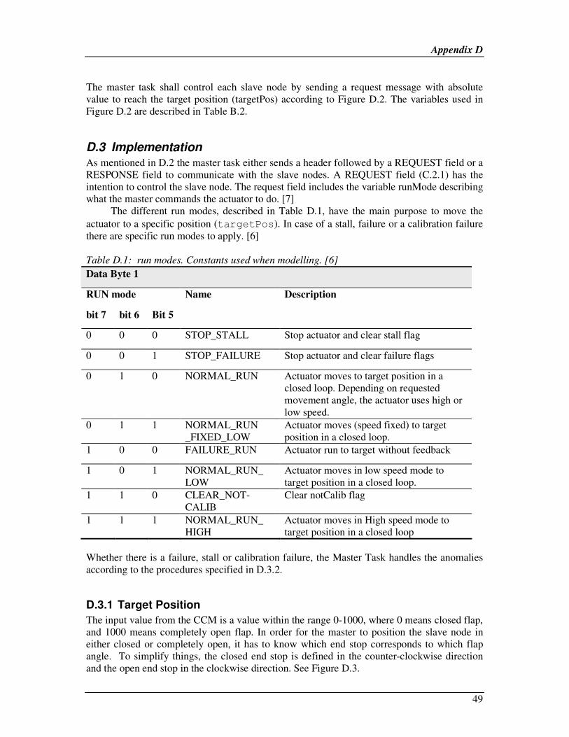
Appendix D

49

The master task shall control each slave node by sending a request message with absolute value to reach the target position (targetPos) according to Figure D.2. The variables used in Figure D.2 are described in Table B.2.

D.3 Implementation

As mentioned in D.2 the master task either sends a header followed by a REQUEST field or a RESPONSE field to communicate with the slave nodes. A REQUEST field (C.2.1) has the intention to control the slave node. The request field includes the variable runMode describing what the master commands the actuator to do. [7]

The different run modes, described in Table D.1, have the main purpose to move the actuator to a specific position (targetPos). In case of a stall, failure or a calibration failure there are specific run modes to apply. [6]

Table D.1: run modes. Constants used when modelling. [6]

Data Byte 1

RUN mode

bit 7 bit 6 Bit 5

Name Description

0 0 0 STOP_STALL Stop actuator and clear stall flag

0 0 1 STOP_FAILURE Stop actuator and clear failure flags

0 1 0 NORMAL_RUN Actuator moves to target position in a closed loop. Depending on requested movement angle, the actuator uses high or low speed.

0 1 1 NORMAL_RUN _FIXED_LOW

Actuator moves (speed fixed) to target position in a closed loop.

1 0 0 FAILURE_RUN Actuator run to target without feedback

1 0 1 NORMAL_RUN_ LOW

Actuator moves in low speed mode to target position in a closed loop.

1 1 0 CLEAR_NOT-CALIB

Clear notCalib flag

1 1 1 NORMAL_RUN_ HIGH

Actuator moves in High speed mode to target position in a closed loop

Whether there is a failure, stall or calibration failure, the Master Task handles the anomalies according to the procedures specified in D.3.2.

D.3.1 Target Position

The input value from the CCM is a value within the range 0-1000, where 0 means closed flap, and 1000 means completely open flap. In order for the master to position the slave node in either closed or completely open, it has to know which end stop corresponds to which flap angle. To simplify things, the closed end stop is defined in the counter-clockwise direction and the open end stop in the clockwise direction. See Figure D.3.

Appendix D

50

Figure D.3: Definition of actuator direction

To be able to move in the absolute range the master task shall perform “Range detection” at least once (done in factory), and store the end positions.[8] The master task calculates the targetPos according to equation below. [6]

( ) 4095mod1000

1argCCM

RangeendPosetPost ⋅+= Equation D.1

D.3.1.1 SWAP FLAG

As mentioned above, based on the actuator position variable in the Master and input value received from the CCM, the Master does a computation of absoulute targetPos. [6]

The actuator calculates the direction from targetPos-actualPos, a negative sign means a decrement direction and positive an incremental direction. [6]

Should the required path crosses the zero,see Figure D.4, a wraparound error occurs. This will make the actuator motor control to miscalculate the direction of targetPos. For example, if the correct direction is incremental, the motor control sets a decrement direction and tries to reach targetPos the other way around. Naturally this is not possible due to the flap mechanics and the actuator gets stuck in an end position of the flap before it has reached targetPos. [6]

Figure D.4: Description of the address wraparound error

Appendix D

51

In case of a predicted direction error, the Master calculates a shifted targetPos and sets the swap flag to 1. The shifted targetPos is equal to targetPos XOR 0x800 and shifts the position half a turn. The set swap flag tells the actuator to calculate a shifted actualPos. These shifted positions are the given positions to the actuator motor control which now performs a correct direction calculation. [6]

Note: When the calculated need of movement (targetPos-actuator position) exceeds a half turn (2048 pos), the master task predicts a faulty direction calculation and sets the swap flag.[8]

D.3.2 Calibration, Stall, Failure procedures

D.3.2.1 Calibration

This procedure is applied by the master when the notCalib flag is set, (see C.2.2.4). The master shall command the actuator to move until the actuator recognizes stall detection. This is done by adding or subtracting (depending on dir flag) 50 positions to the realtive move in order for the actuator to reach the end stop at full speed. This is to reach constant torque to ensure correct stall detection. When the stall flag has been reset by the stall procedure (see below), the master should request the run mode CLEAR_NOT-CALIB. This procedure is called calibration in the master task. [6]

Figure D.5: Principle of calibration procedure

Note: When the flap reaches end position, it can bounce back and continue to move in the opposite direction, back in the range towards the other end position. The actuator does not recognize the direction change and the stall flag is not set. This means that the actuator reports that its actualPos is 50 pos beyond the end stop, when it is actually 50 pos from the end stop and still inside the range. The recommended procedure is to move 100 pos at a time in the initial direction until a stall is recognized. This stall position is the new end reference point and the other is calculated using the dir flag and the stored range value. [6]

D.3.2.2 Stall

A stall status is set by the actuator motor control when the torque reaches a defined stall limit. The actuator will stop and all normal run modes are disabled, only FAILURE_RUN mode is allowed. The procedure after a stall is illustrated in Figure D.6 [6]

A stall detected inside the “gray zone” should be set as a new end reference position and the other end stop will be set using the dir flag and the stored range value. [6]

A stall detected outside the “gray zone” should be handled as a “hard flap point” and is to be ignored. A recommendation is to request STOP_STALL, move backwards a few positions and then push trough the stall area in NORMAL_RUN (this is implemented in the

Appendix D

52

figure below). Another recommendation is to directly push through the stall area in FAILURE_RUN and after that request STOP_STALL to continue in a NORMAL_RUN mode.[6]

Figure D.6: Principle of stall handling

D.3.2.3 Failure

If the master recognizes a failure through the failure register, the actuator has halted. There are eight different failure flags, and they are thoroughly described in Table C.9. The solution to each failure is similar and is described in General Solution below. There are some exceptions which are described in the header Exceptions below. In every failure, except when bit #3 in the Failure_Register is set, the notCalib flag is set. The notCalib flag remains set until all (except bit #3) failure flags are cleared and the master task has required the run mode CLEAR_NOT-CALIB. [6]

General Solution

The general idea to solve the failure is for the master to send a request with the run mode STOP_FAILURE. Next thing is to wait in this mode until the failure flags are cleared. The notCalib flag is set, and the master should request a calibration routine as described above. [6]

Exceptions

Some failures are handled differently than the procedure described above. With the run mode FAILURE_RUN it is possible to make the actuator move even if a failure flag is raised. It is recommended not to request to run to end stop with this command, it may break the flap and loose accuracy. [6]

When bit #7 is set in the failuire register the general solution is used. But if the flag remains set after some a certain timeout, then the master should assume that this failure is permanent and should use the run mode FAILURE_RUN to move the actuator. [6]

When bit #3 is set, it means that a communication failure has occurred. The request to clear this failure should have the lowest priority, because this flag does not inhibit any functionality. The notCalib flag is not set when this failure is triggered. [6]

When bit #2 is set in the Failure_Register a special routine should be applied: After the general solution has been applied, try to run the actuator in the same direction. Repeat this routine 4 times if the same failure occurs. If the flag is still set use the general solution but try to run in the opposite direction (≥17 pos) once. If the failure flag is set again immediately run in FAILURE_RUN until power off. [6]