Modeling aquatic invasions and control in a lake system: principles and approaches

Alex PotapovCentre for Mathematical Biology, University of Alberta

and Lodge Lab, University of Notre Dame http://www.math.ualberta.ca/~apotapov/

Joint work with M. Lewis and D. Finnoff

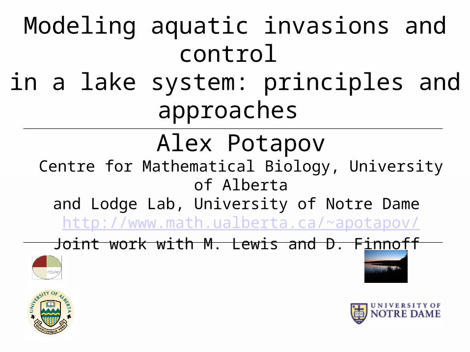
Sea Lamprey

Zebra Mussels

Motivation: Great Lakes Invasion

Rusty crayfish

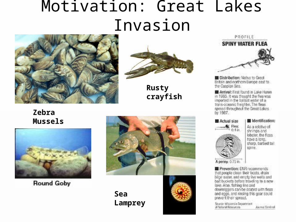
Economic and ecological damage from the invaders

Zebra mussels

Clog water pipes and water treatment facilities; yearly cost/facility ~$80,000-800,000

Ecological damage

Sea Lamprey

1 Adult kills about 40 fishes

In 1920s decreased fish harvest in GL about 50 times

Spiny waterflea

Collect on fishing equipment, may damage it.

No predators Consume lots of plankton

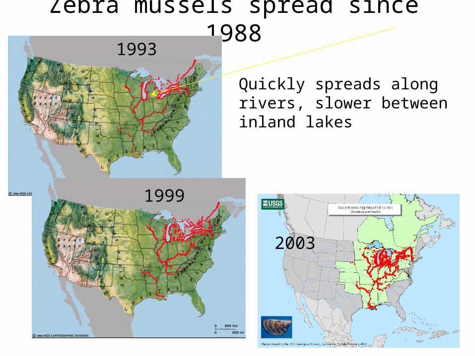
Zebra mussels spread since 1988

Quickly spreads along rivers, slower between inland lakes

1993

1999

2003

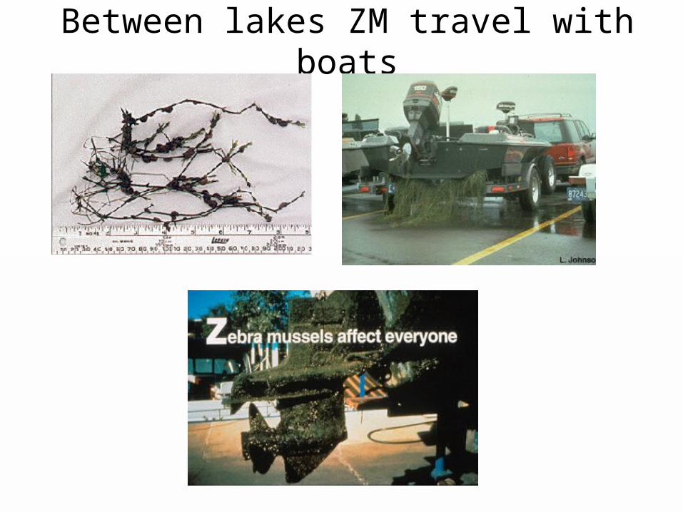
Between lakes ZM travel with boats

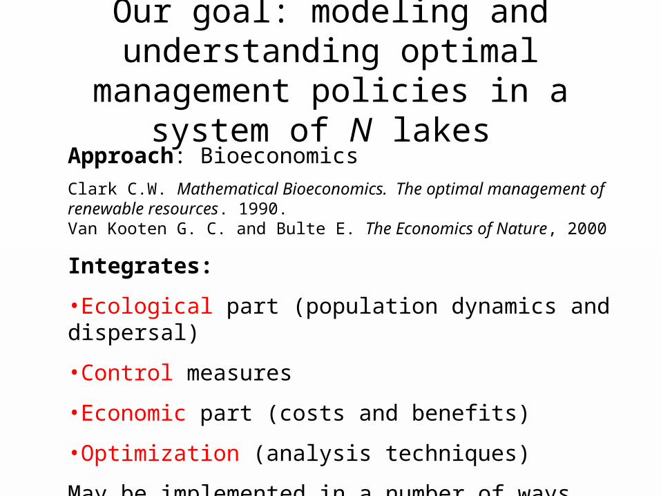
Our goal: modeling and understanding optimal management policies in a system

of N lakes Approach: Bioeconomics

Clark C.W. Mathematical Bioeconomics. The optimal management of renewable resources. 1990.Van Kooten G. C. and Bulte E. The Economics of Nature, 2000

Integrates:

•Ecological part (population dynamics and dispersal)

•Control measures

•Economic part (costs and benefits)

•Optimization (analysis techniques)

May be implemented in a number of ways

Possible model types

What details to be included?

What kind of model to be chosen?

Main choices:

Regional scale – Lake scale

Deterministic – Stochastic

Continuous – Discrete

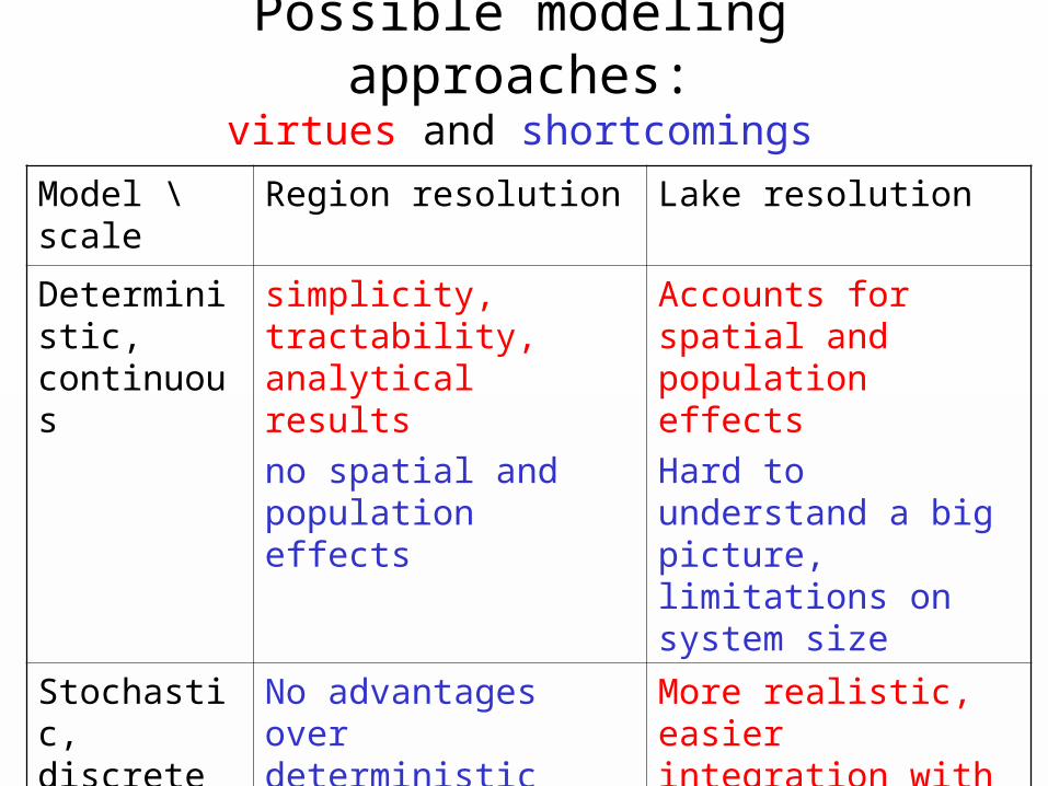
Possible modeling approaches:virtues and shortcomings

Model \ scale Region resolution Lake resolution

Deterministic, continuous

simplicity, tractability, analytical results

no spatial and population effects

Accounts for spatial and population effects

Hard to understand a big picture, limitations on system size

Stochastic, discrete

No advantages over deterministic models

More realistic, easier integration with other ecological concepts

Serious limitations on system size

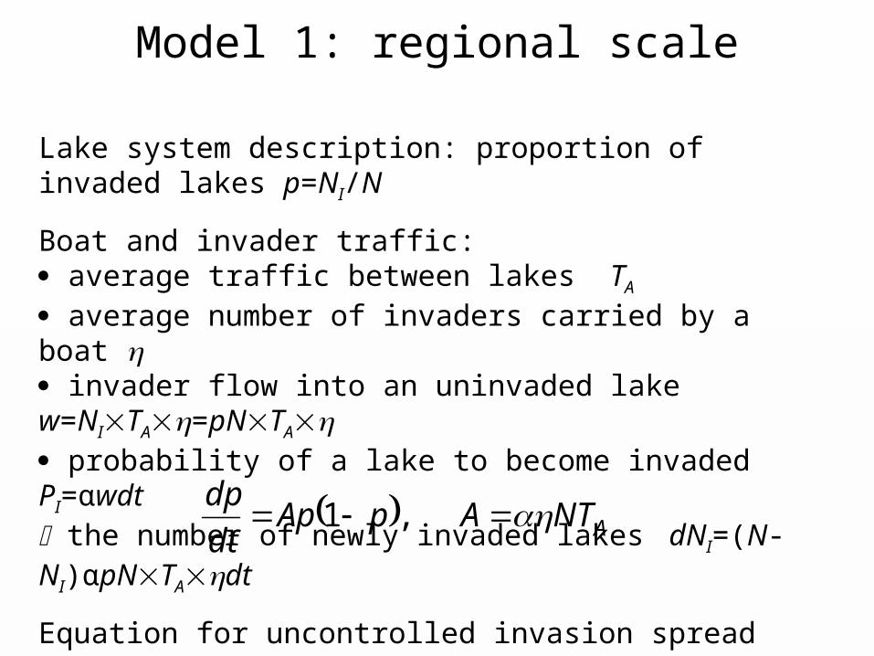
Model 1: regional scale

Lake system description: proportion of invaded lakes p=NI/N

Boat and invader traffic: average traffic between lakes TA average number of invaders carried by a boat invader flow into an uninvaded lake w=NITA=pNTA probability of a lake to become invaded PI=αwdt the number of newly invaded lakes dNI=(N-NI)αpNTAdt

Equation for uncontrolled invasion spread ANTApApdt

dp ,1

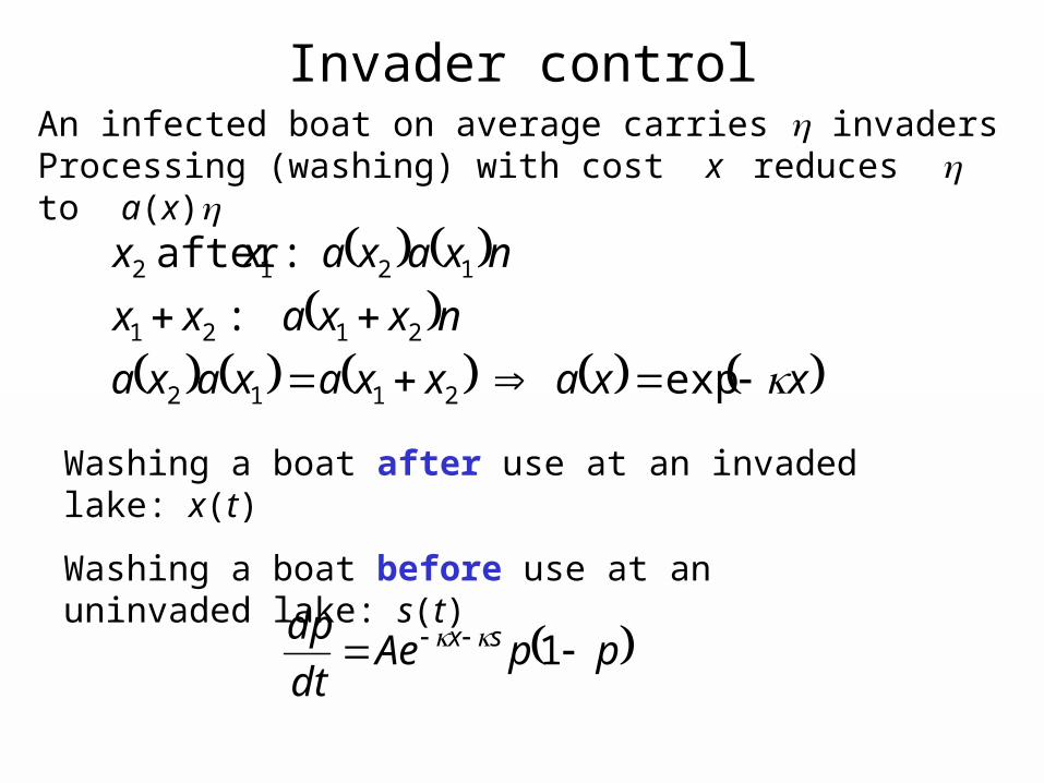
Invader controlAn infected boat on average carries invadersProcessing (washing) with cost x reduces to a(x)

xxaxxaxaxa

nxxaxx

nxaxaxx

exp

:

:after

2112

2121

1212

Washing a boat after use at an invaded lake: x(t)

Washing a boat before use at an uninvaded lake: s(t)

ppAedt

dp sx 1

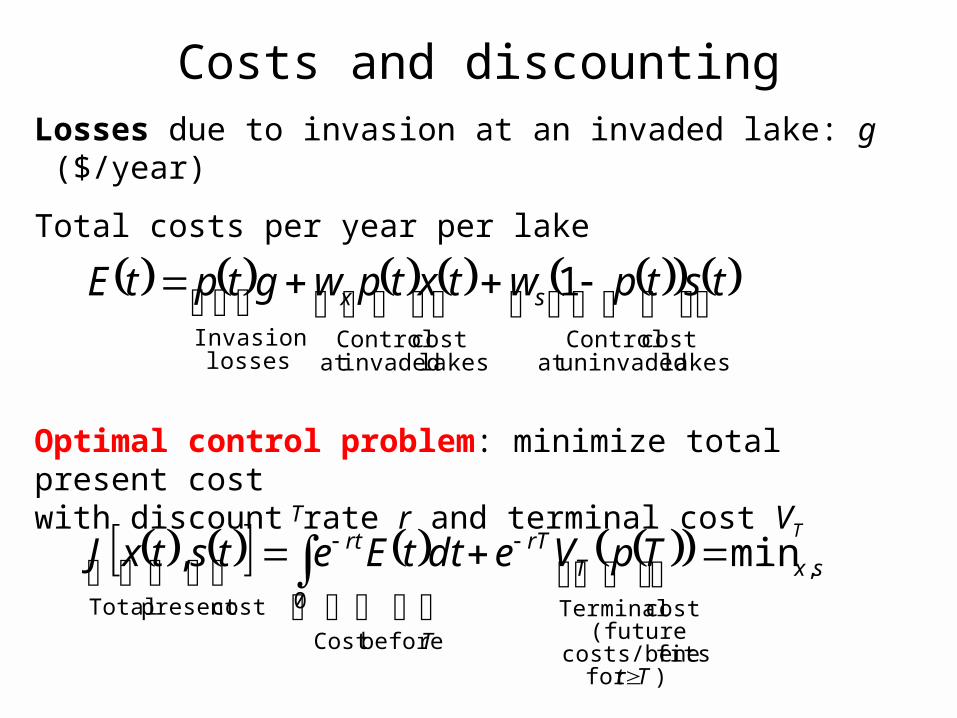
Losses due to invasion at an invaded lake: g ($/year)

Total costs per year per lake

Costs and discounting

sx

Tt

TrT

T

Trt TpVedttEetstxJ ,

)for fitscosts/bene (futurecost Terminal

beforeCost

0costpresent Total

min,

lakes uninvadedat

cost Controllakes invadedat

cost Controllosses

Invasion

1 tstpwtxtpwgtptE sx

Optimal control problem: minimize total present cost with discount rate r and terminal cost VT

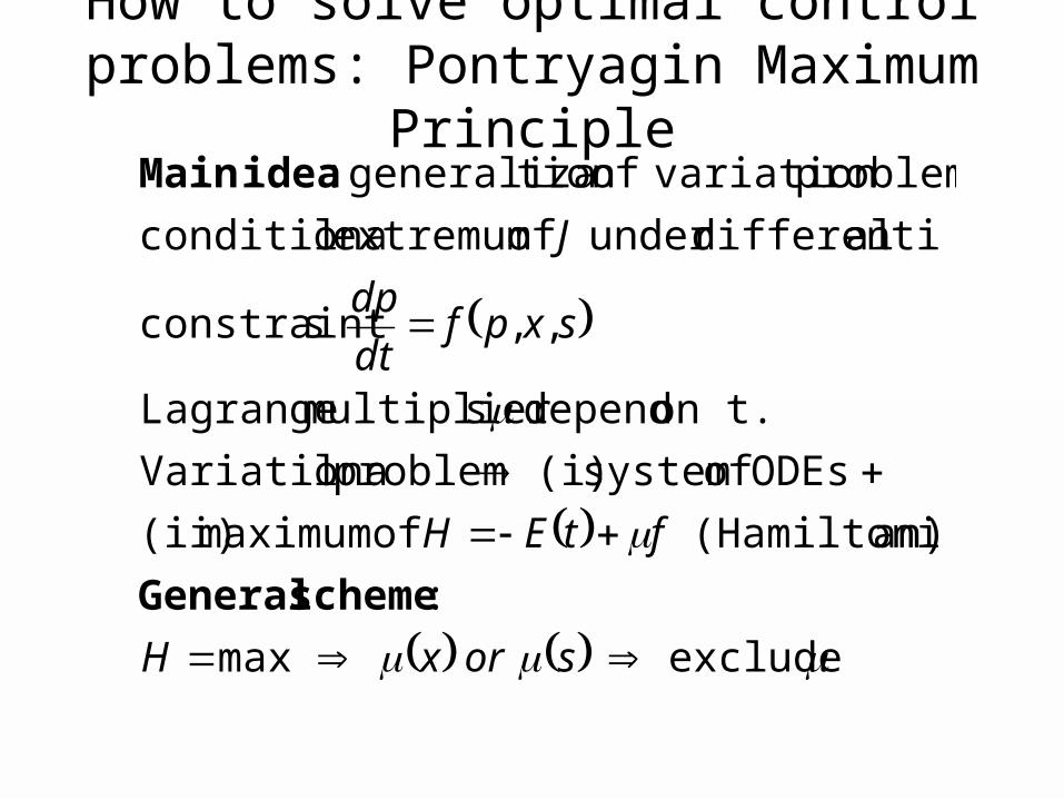
How to solve optimal control problems: Pontryagin Maximum Principle

exclude max

:

an)(Hamiltoni of maximum (ii)

ODEs of system (i) problem lVariationa

on t. depend smultiplier Lagrange

,, sconstraint

aldifferentiunder of extremum lconditiona

problem, variationoftion generaliza :

sorxH

ftEH

sxpfdt

dp

J

scheme General

idea Main

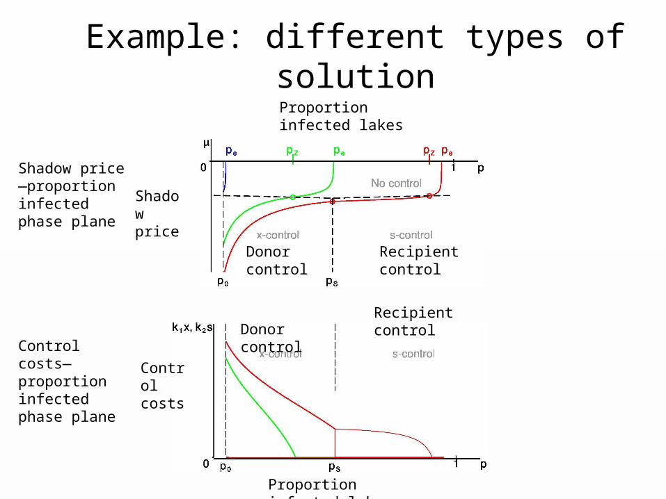
Shadow price

Proportion infected lakes

Proportion infected lakes

Control costs

Donor controlRecipient control

Recipient controlDonor control

Example: different types of solution

Control costs—proportion infected phase plane

Shadow price—proportion infected phase plane

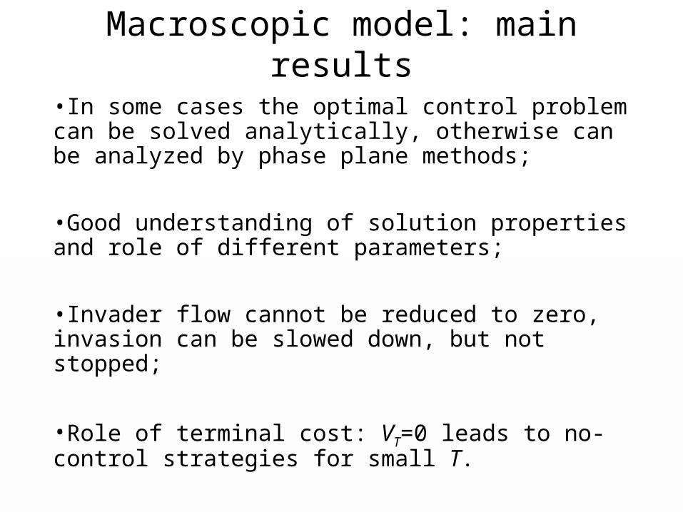
Macroscopic model: main results

•In some cases the optimal control problem can be solved analytically, otherwise can be analyzed by phase plane methods;

•Good understanding of solution properties and role of different parameters;

•Invader flow cannot be reduced to zero, invasion can be slowed down, but not stopped;

•Role of terminal cost: VT=0 leads to no-control strategies for small T.

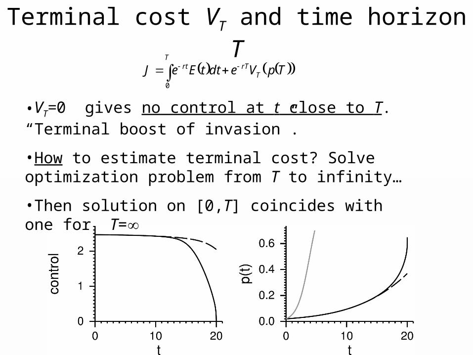
Terminal cost VT and time horizon T

•VT=0 gives no control at t close to T. “Terminal boost of invasion”.

•How to estimate terminal cost? Solve optimization problem from T to infinity…

•Then solution on [0,T] coincides with one for T=

TpVedttEeJ TrT

Trt

0

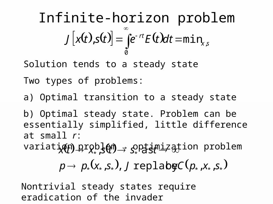
Infinite-horizon problem

sxrt dttEetstxJ ,

0

min,

Solution tends to a steady state

Two types of problems:

a) Optimal transition to a steady state

b) Optimal steady state. Problem can be essentially simplified, little difference at small r: variation problem → optimization problem

******

**

,,by replace,,

as,

sxpCJsxpp

tstsxtx

Nontrivial steady states require eradication of the invader

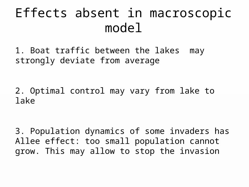
Effects absent in macroscopic model

1. Boat traffic between the lakes may strongly deviate from average

2. Optimal control may vary from lake to lake

3. Population dynamics of some invaders has Allee effect: too small population cannot grow. This may allow to stop the invasion

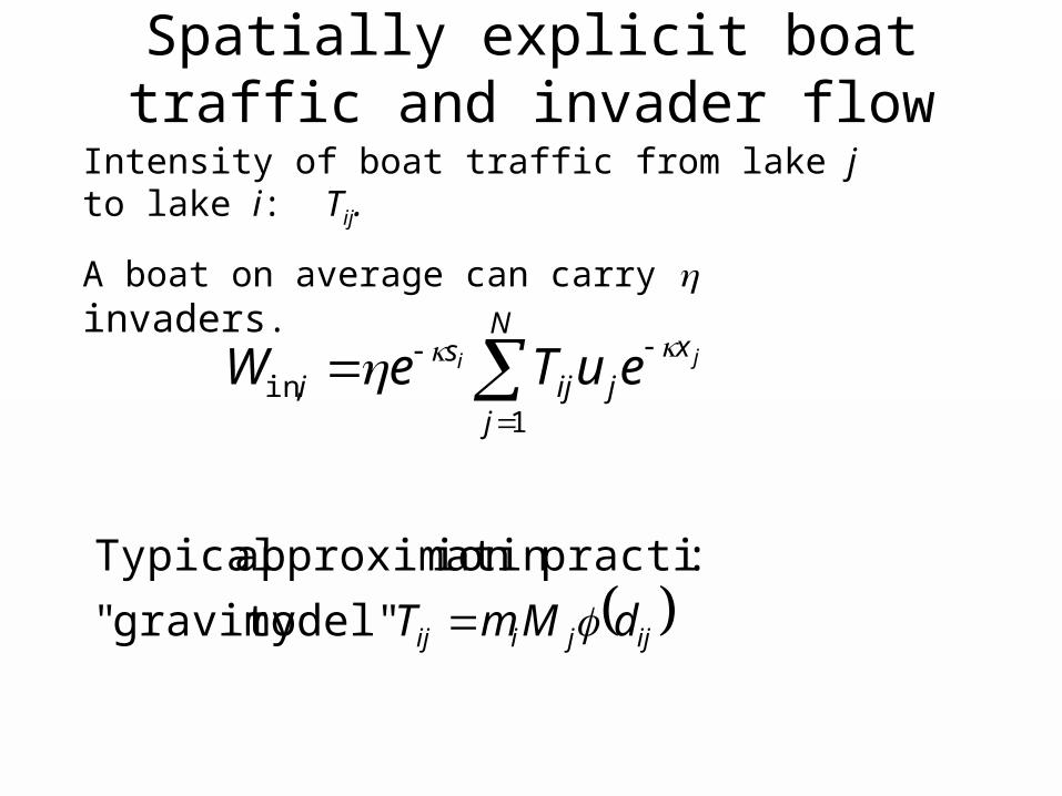
Spatially explicit boat traffic and invader flow

Intensity of boat traffic from lake j to lake i: Tij.

A boat on average can carry invaders.

jix

N

jjij

si euTeW

1

,in

ijjiij dMmT model"gravity "

:practicein ion approximat Typical

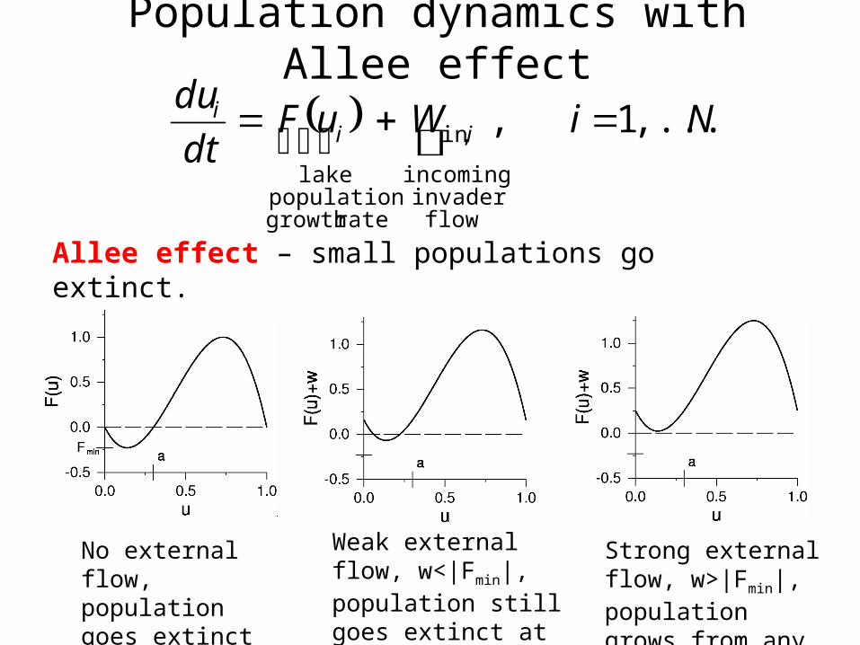
Population dynamics with Allee effect

NiWuFdt

duii

i ,...,1,

flowinvader

incoming

,in

rategrowth population

lake

No external flow, population goes extinct at small u

Weak external flow, w<|Fmin|, population still goes extinct at small u;

Strong external flow, w>|Fmin|, population grows from any u

Allee effect – small populations go extinct.

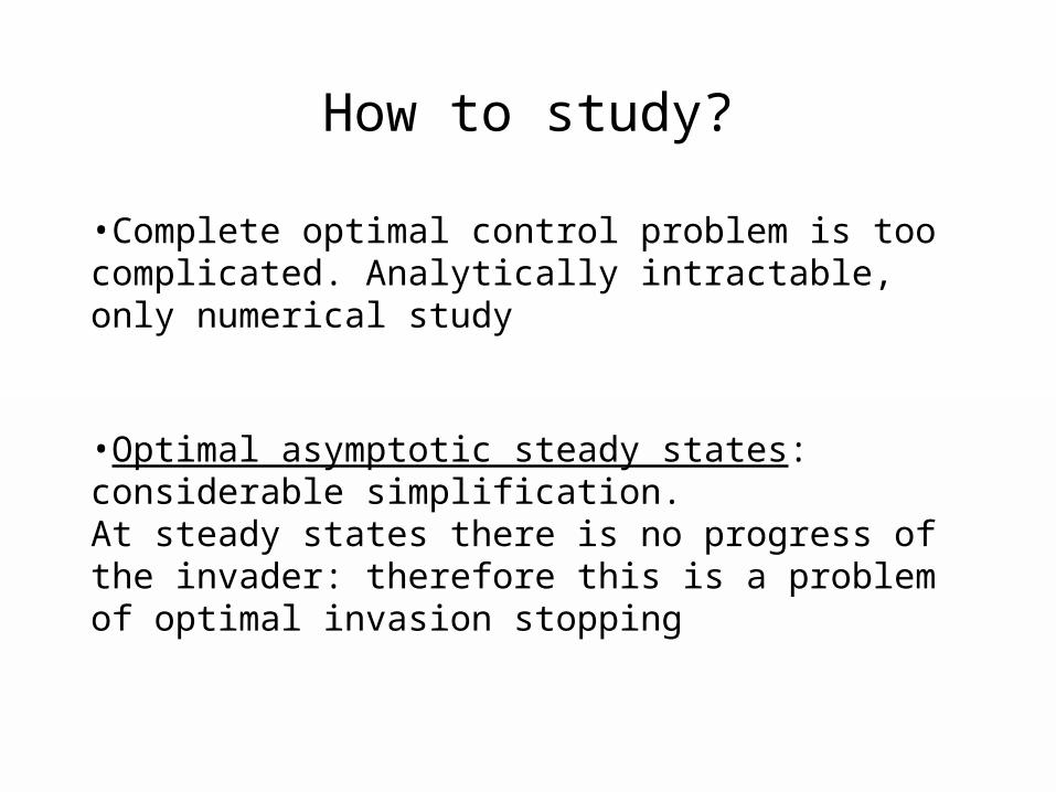
•Complete optimal control problem is too complicated. Analytically intractable, only numerical study

•Optimal asymptotic steady states: considerable simplification.At steady states there is no progress of the invader: therefore this is a problem of optimal invasion stopping

How to study?

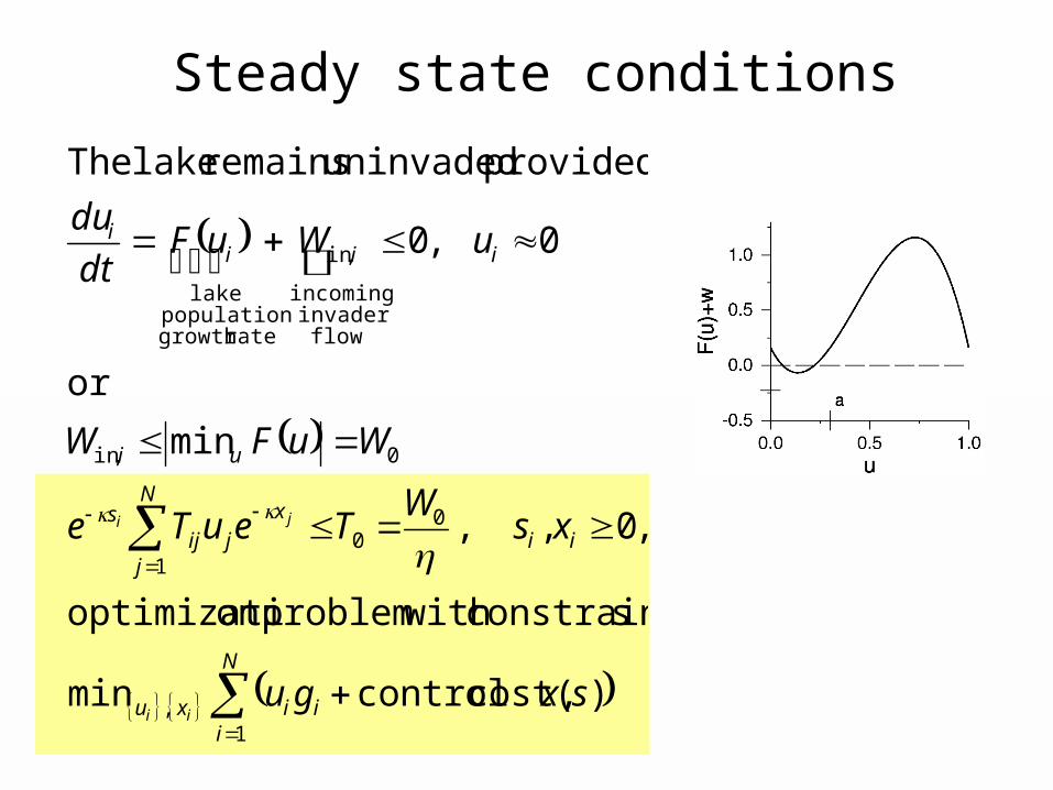
Steady state conditions

N

iiixu

iix

N

jjij

s

ui

iiii

sxgu

xsW

TeuTe

WuFW

uWuFdt

du

ii

ji

1,

00

1

0,in

flowinvader

incoming

,in

rategrowth population

lake

),cost( controlmin

sconstraint with problemon optimizati

,0,,

min

or

0,0

provided uninvaded remains lake The

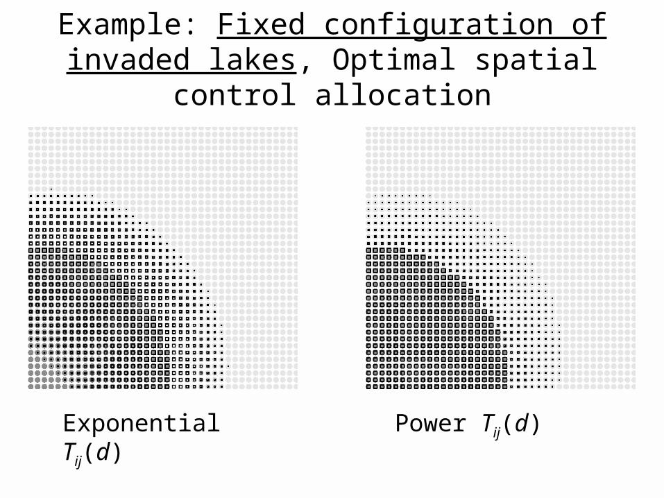
Example: Fixed configuration of invaded lakes, Optimal spatial control allocation

Exponential Tij(d) Power Tij(d)

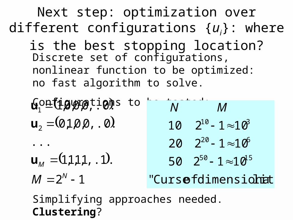
Next step: optimization over different configurations {ui}: where is the best stopping location?

Discrete set of configurations, nonlinear function to be optimized: no fast algorithm to solve.

Configurations to be tested:

12

1,...,1,1,1,1

...

0,...,0,0,1,0

0,...,0,0,0,1

2

1

N

M

M

u

u

u

lity"dimensiona of Curse"

1012

1012

1012

50

20

10

1550

620

310

MN

Simplifying approaches needed. Clustering?

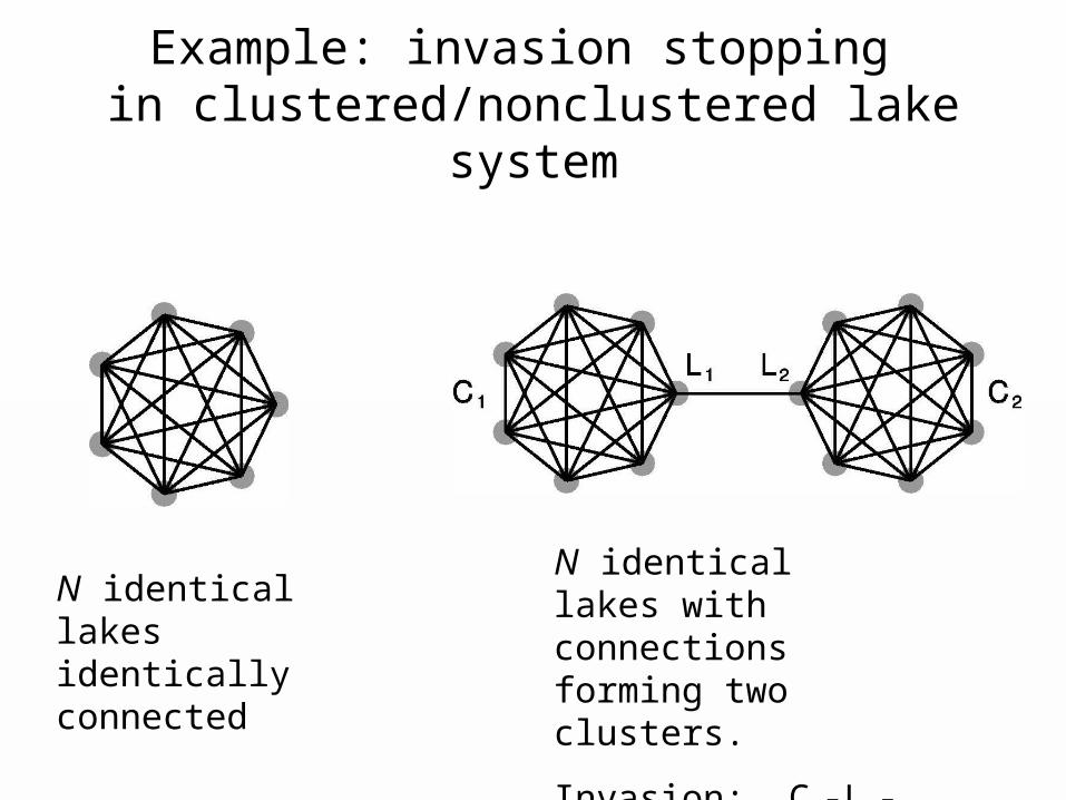
Example: invasion stopping in clustered/nonclustered lake system

N identical lakes identically connected

N identical lakes with connections forming two clusters.

Invasion: C1-L1-L2-C2

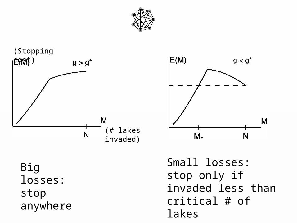
Big losses: stop anywhere

Small losses: stop only if invaded less than critical # of lakes

(Stopping cost)

(# lakes invaded)

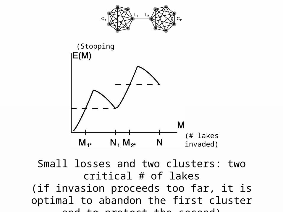
Small losses and two clusters: two critical # of lakes(if invasion proceeds too far, it is optimal to abandon

the first cluster and to protect the second)

(Stopping cost)

(# lakes invaded)

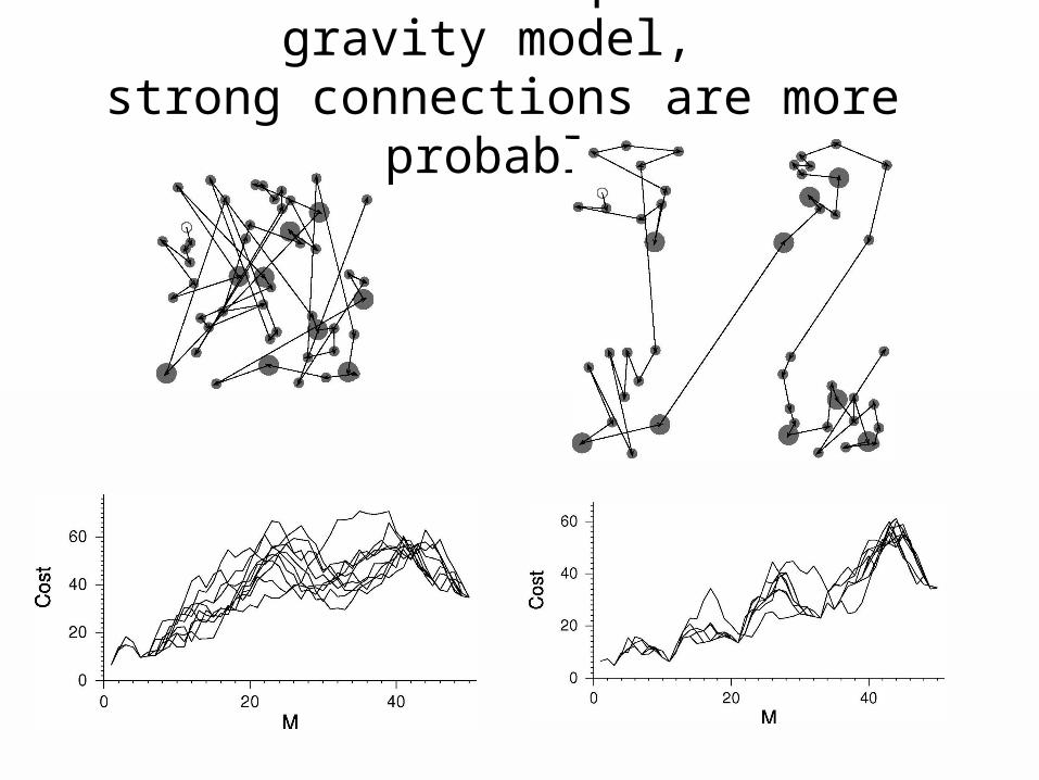
Random invasion paths in a gravity model, strong connections are more probable

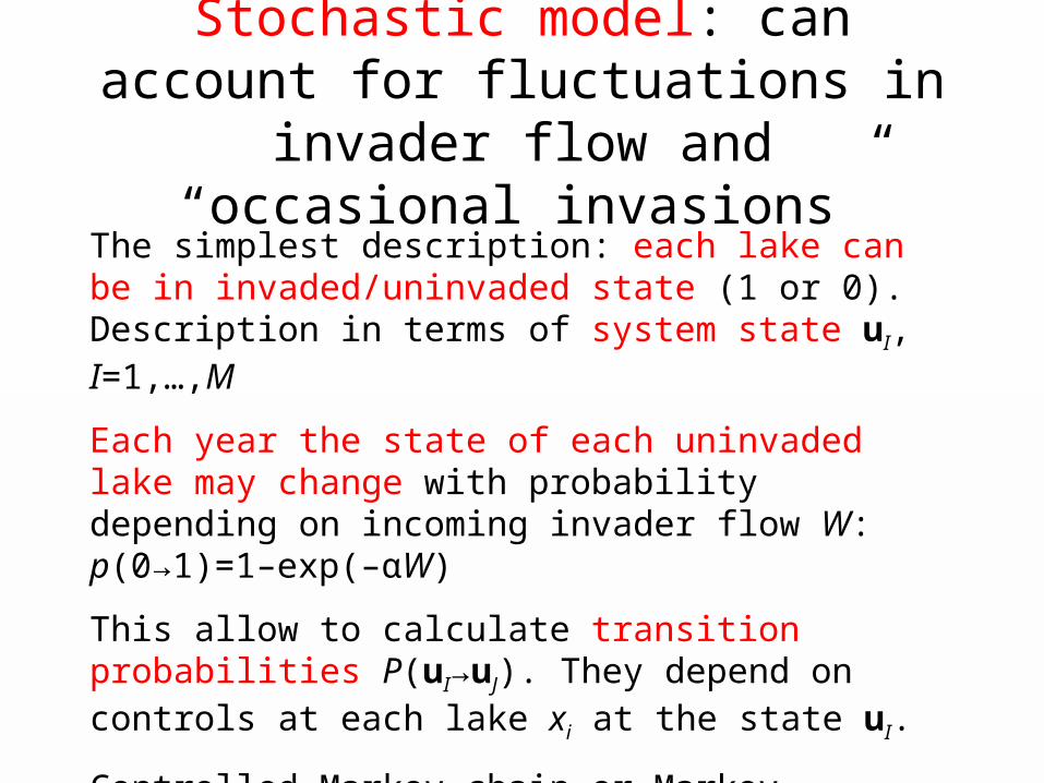
Stochastic model: can account for fluctuations in invader flow and

“occasional invasions”The simplest description: each lake can be in invaded/uninvaded state (1 or 0). Description in terms of system state uI, I=1,…,M

Each year the state of each uninvaded lake may change with probability depending on incoming invader flow W: p(0→1)=1–exp(–αW)

This allow to calculate transition probabilities P(uI→uJ). They depend on controls at each lake xi at the state uI.

Controlled Markov chain or Markov decision process

Optimal solution: minimizes total average costs

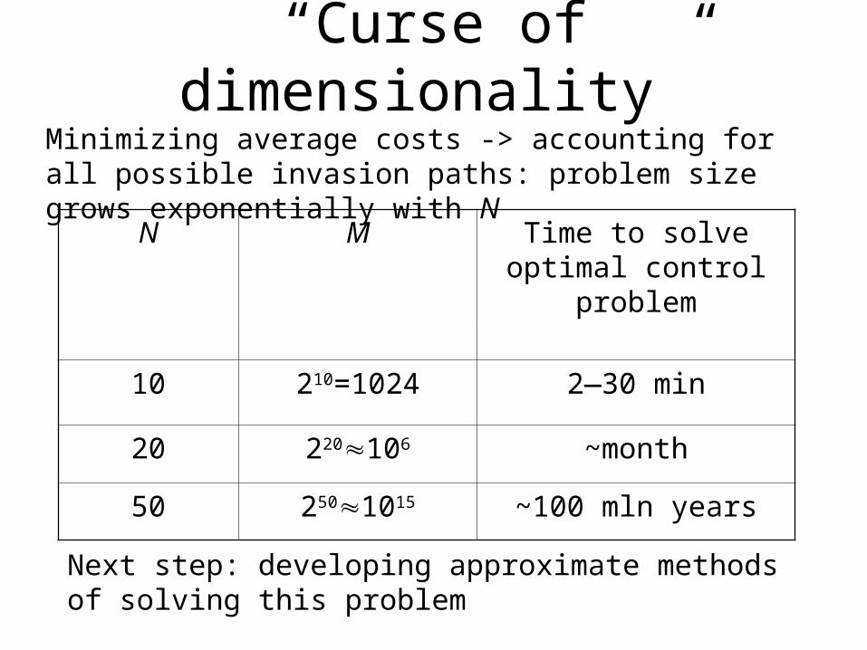
“Curse of dimensionality”

N M Time to solve optimal control problem

10 210=1024 2—30 min

20 220106 ~month

50 2501015 ~100 mln years

Minimizing average costs -> accounting for all possible invasion paths: problem size grows exponentially with N

Next step: developing approximate methods of solving this problem

Conclusions

• Spectrum of models allows us to understand different sides of models•Simple averaged models show global picture and allows us better setting up more detailed problems•Lake-scale models account for local features of population dynamics and transportation•Considering of optimal steady states allows considerable simplification: from optimal control to optimization•Stochastic problems are more realistic but much harder to solve

Acknowledgements ISIS project, (NSF DEB 02-13698) NSERC Collaboration Research Opportunity grant.

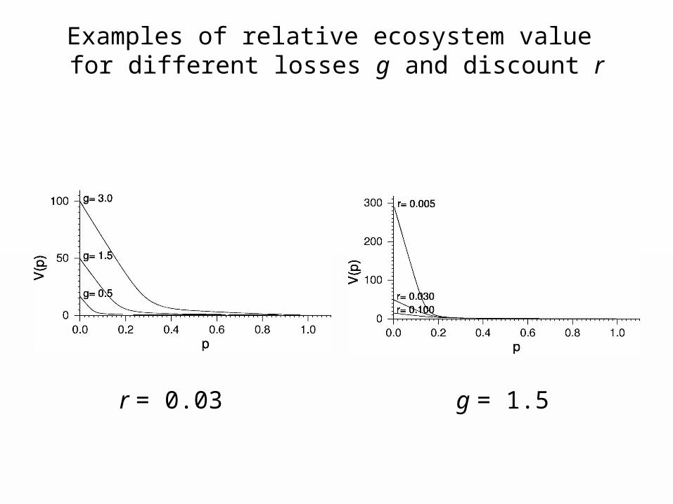
Examples of relative ecosystem value for different losses g and discount r

r = 0.03 g = 1.5