1

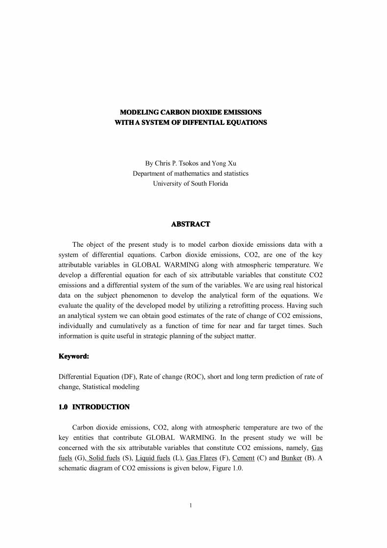
MODELINGMODELINGMODELINGMODELING CARBONCARBONCARBONCARBON DIOXIDEDIOXIDEDIOXIDEDIOXIDE EMISSIONSEMISSIONSEMISSIONSEMISSIONSWITHWITHWITHWITHAAAA SYSTEMSYSTEMSYSTEMSYSTEMOFOFOFOFDIFFENTIALDIFFENTIALDIFFENTIALDIFFENTIAL EQUATIONSEQUATIONSEQUATIONSEQUATIONS

By Chris P. Tsokos and Yong XuDepartment of mathematics and statistics

University of South Florida

ABSTRACTABSTRACTABSTRACTABSTRACT

The object of the present study is to model carbon dioxide emissions data with asystem of differential equations. Carbon dioxide emissions, CO2, are one of the keyattributable variables in GLOBAL WARMING along with atmospheric temperature. Wedevelop a differential equation for each of six attributable variables that constitute CO2emissions and a differential system of the sum of the variables. We are using real historicaldata on the subject phenomenon to develop the analytical form of the equations. Weevaluate the quality of the developed model by utilizing a retrofitting process. Having suchan analytical system we can obtain good estimates of the rate of change of CO2 emissions,individually and cumulatively as a function of time for near and far target times. Suchinformation is quite useful in strategic planning of the subject matter.

Keyword:Keyword:Keyword:Keyword:

Differential Equation (DF), Rate of change (ROC), short and long term prediction of rate ofchange, Statistical modeling

1.01.01.01.0 INTRODUCTIONINTRODUCTIONINTRODUCTIONINTRODUCTION

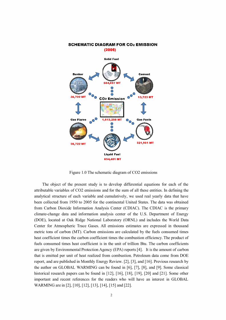
Carbon dioxide emissions, CO2, along with atmospheric temperature are two of thekey entities that contribute GLOBAL WARMING. In the present study we will beconcerned with the six attributable variables that constitute CO2 emissions, namely, Gasfuels (G), Solid fuels (S), Liquid fuels (L), Gas Flares (F), Cement (C) and Bunker (B). Aschematic diagram of CO2 emissions is given below, Figure 1.0.

2

Figure 1.0 The schematic diagram of CO2 emissions

The object of the present study is to develop differential equations for each of theattributable variables of CO2 emissions and for the sum of all these entities. In defining theanalytical structure of each variable and cumulatively, we used real yearly data that havebeen collected from 1950 to 2005 for the continental United States. The data was obtainedfrom Carbon Dioxide Information Analysis Center (CDIAC). The CDIAC is the primaryclimate-change data and information analysis center of the U.S. Department of Energy(DOE), located at Oak Ridge National Laboratory (ORNL) and includes the World DataCenter for Atmospheric Trace Gases. All emissions estimates are expressed in thousandmetric tons of carbon (MT). Carbon emissions are calculated by the fuels consumed timesheat coefficient times the carbon coefficient times the combustion efficiency. The product offuels consumed times heat coefficient is in the unit of trillion Btu. The carbon coefficientsare given by Environmental Protection Agency (EPA) reports [4]. It is the amount of carbonthat is emitted per unit of heat realized from combustion. Petroleum data come from DOEreport, and are published in Monthly Energy Review. [2], [3], and [16]. Previous research bythe author on GLOBAL WARMING can be found in [6], [7], [8], and [9]. Some classicalhistorical research papers can be found in [12], [16], [18], [19], [20] and [21]. Some otherimportant and recent references for the readers who will have an interest in GLOBALWARMING are in [2], [10], [12], [13], [14], [15] and [22].

3

2.2.2.2.0000ANALYTICALANALYTICALANALYTICALANALYTICALDEVELOPMENTSDEVELOPMENTSDEVELOPMENTSDEVELOPMENTSThomas J. Goreau, [20], in 1990 briefly mentioned that the rate of change of CO2

emissions and also CO2 in the atmosphere should be studied using differential equations.However, to our knowledge no actual differential equations have been developed on thesubject matter to study the rate of change of CO2.

Using E to represent CO2 emissions and the systematic representation of the sixattributable variables, the functional form of the differential equations is given by equation2.1 below.

(2.1)( ) ( ) ( ) ( ) ( ) ( ) ( )( , , , , , )d E d G d S d L d F d C d Bfdt dt dt dt dt dt dt

=

Without loss of generality, we can express the rate of change of CO2 emissions as afunction of time by

(2. 2)1 2 3 4 5 6 7( ) ( ) ( ) ( ) ( ) ( ) ( )d E d G d S d L d F d C d BC C C C C C Cdt dt dt dt dt dt dt

= + + + + + +

where C1 to C6 are the coefficients of each differential term and C7 is a constant. Weshall begin to formulate the differential equations of each attributable variable.

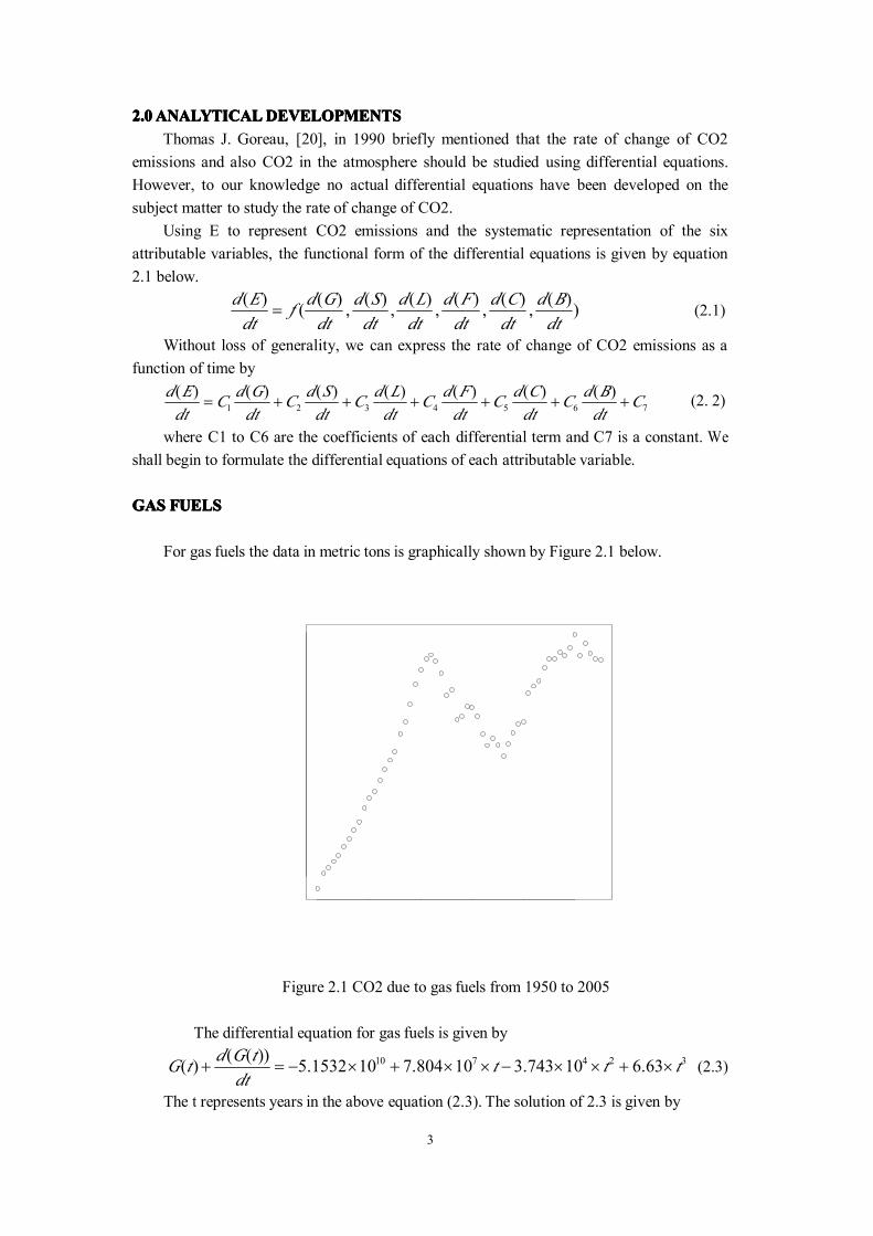
GASGASGASGAS FUELSFUELSFUELSFUELS

For gas fuels the data in metric tons is graphically shown by Figure 2.1 below.

1950 1960 1970 1980 1990 2000

1000

0015

0000

2000

0025

0000

3000

0035

0000

Year

Gas

Fue

ls

Figure 2.1 CO2 due to gas fuels from 1950 to 2005

The differential equation for gas fuels is given by

(2.3)10 7 4 2 3( ( ))( ) 5.1532 10 7.804 10 3.743 10 6.63d G tG t t t tdt

+ = − × + × × − × × + ×

The t represents years in the above equation (2.3). The solution of 2.3 is given by

4

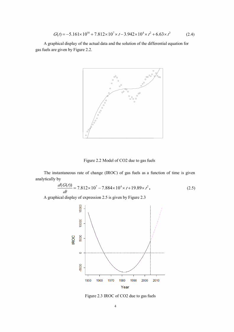
(2.4)10 7 4 2 3( ) 5.161 10 7.812 10 3.942 10 6.63G t t t t= − × + × × − × × + ×

A graphical display of the actual data and the solution of the differential equation forgas fuels are given by Figure 2.2.

1950 1960 1970 1980 1990 2000

1000

0015

0000

2000

0025

0000

3000

0035

0000

Year

Gas

Fue

ls

Figure 2.2 Model of CO2 due to gas fuels

The instantaneous rate of change (IROC) of gas fuels as a function of time is givenanalytically by

.... (2.5)7 4 2( ( )) 7.812 10 7.884 10 19.89d G t t tdt

= × − × × + ×

A graphical display of expression 2.5 is given by Figure 2.3

Figure 2.3 IROC of CO2 due to gas fuels

5

Thus one can utilize either equation 2.5 on the above graph to obtain the estimate of therate of change for CO2 due to gas fuels for short and long terms of time. The question is howgood are these estimates? The answer depends on the quality of the developed analyticalmodels using the raw data. To test for the quality of the proposed analytical models, we usethree statistical criteria, the ( adjusted), the PRESS statistic and residual analysis.2R 2R

The regression sum of squares (SSR), also called the explained sum of squares, is thevariation that is explained by the regression model. The sum of squared errors (SSE), alsocalled the residual sum of squares, is the variation that is left unexplained. The total sum ofsquares (SST) is proportional to the sample variance and equals the sum of SSR and SSE.The coefficient of determination is defined as the proportion of the total response2Rvariation that is explained by the model. It provides an overall measure of how well themodel fits. adjusted will adjust for degree of freedom of the model and it works better2Rwhen we have a lot of parameters. The prediction of residual error sum of squares (PRESS)statistics will evaluate how good the estimation will be if each time we remove one data [5].

The calculated values for the gas fuel model for ( adjusted) and PRESS statistic2R 2Rare given by Table 2.1, below.

Table 2.1 statistical evaluation criteria

The values of ( adjusted) reflect the fact that we have identified a good model2R 2Ralong with a PRESS statistic value that is the smallest of several models that we tested.Furthermore, the residual analysis we performed on the proposed differential equation of gasfuels is given in Table 2.2, below

Table 2.2 Residual analysis

Here, the empirical rate of change, Empirical ROC, is calculated using the actual data of

R square R square adjusted PRESS0.8493 0.8406 49633871512

Year Empirical ROC DF IROC residual1996 0.0007889168 0.01297814 -0.0121892211997 0.02146635 0.01470999 0.0067563671998 -0.01184225 0.01649996 -0.0283422141999 0.02542004 0.01833330 0.0070867392000 0.03846016 0.02019471 0.0182654532001 -0.06112036 0.02206862 -0.0831889782002 0.03976228 0.02393955 0.0158227382003 -0.03174238 0.02579240 -0.0575347802004 -0.01472101 0.02761275 -0.0423337532005 -0.00573488 0.02938714 -0.035122018

Mean of residual -0.02107797Standard deviation of residual (SD) 0.03406736Standard error of residual (SE) 0.01077305

6

gas fuels that we refer to as the true values and the instantaneous rate of change using thedeveloped differential equation, DF IROC, with the residual being the difference of the two.As seen from the table, the residuals are extremely small and so is the standard error. Theseresults attest to the good quality of the proposed model for gas fuels. Thus, in Table 2.3,below, we have calculated 10, 20 and 50 years ahead the instantaneous rate of change of gasfuel emissions.

Table 2.3 future estimation of IROC of CO2 due to gas fuels

LIQUIDLIQUIDLIQUIDLIQUIDFUELSFUELSFUELSFUELS

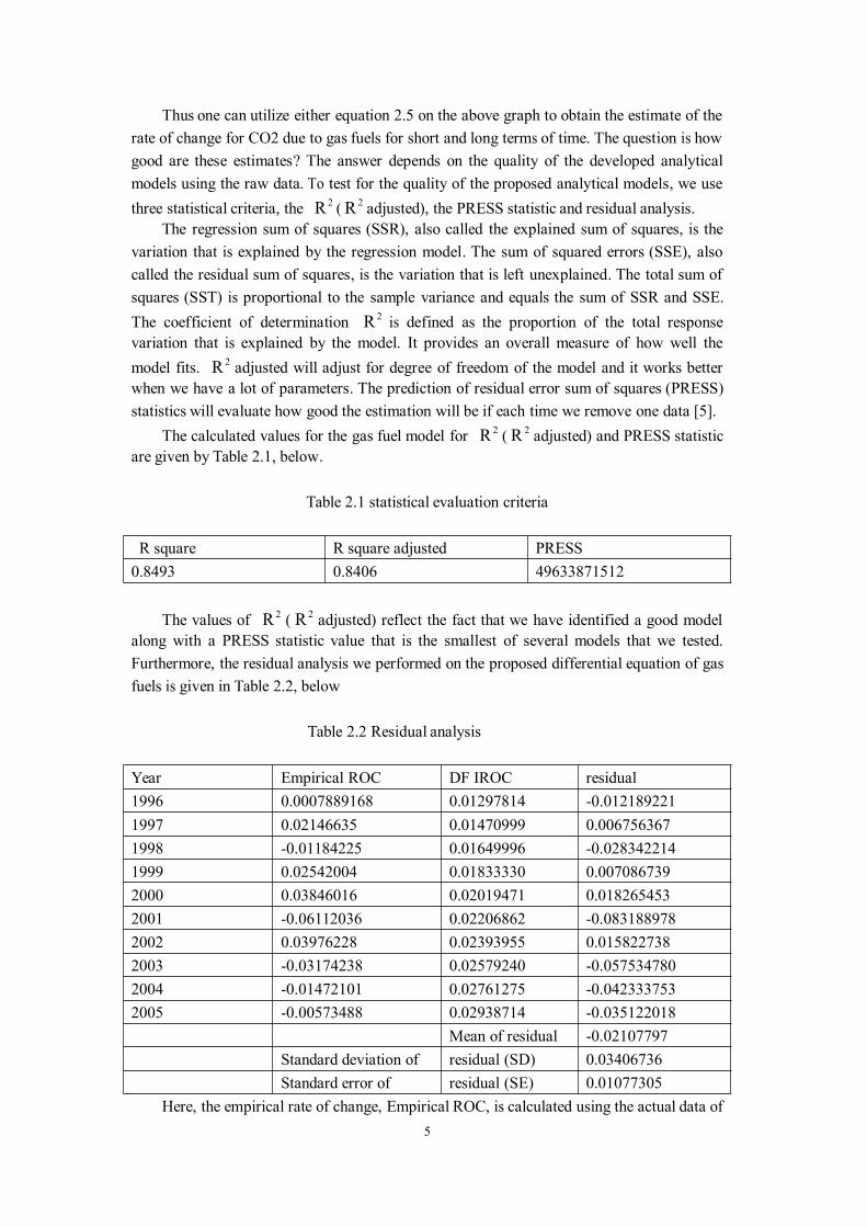
For liquid fuels the data in metric tons is graphically shown by Figure 2.4 below.

1950 1960 1970 1980 1990 2000

3e+0

54e

+05

5e+0

56e

+05

Year

Liqu

id F

uels

Figure 2.4 CO2 due to liquid fuels from 1950 to 2005

The differential equation for liquid fuels is given by

. (2.6)' 10 7 4 2 3( ) ( ) 3.2471 10 4.8971 10 2.4506 10 4.126L t L t t t t+ = − × + × × − × × + ×

The solution of 2.6 is given by

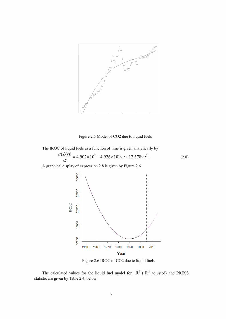
. (2.7)10 7 4 2 3( ) 3.252 10 4.902 10 2.463 10 4.126L t t t t= − × + × × − × × + ×

A graphical display of the actual data and the solution of the differential equation forliquid fuels are given by Figure 2.5

Years 10 years 20 years 50 yearsIROC in future 15275.25 30431.25 99767.25

7

1950 1960 1970 1980 1990 2000

3e+0

54e

+05

5e+0

56e

+05

Year

Liqu

id F

uels

Figure 2.5 Model of CO2 due to liquid fuels

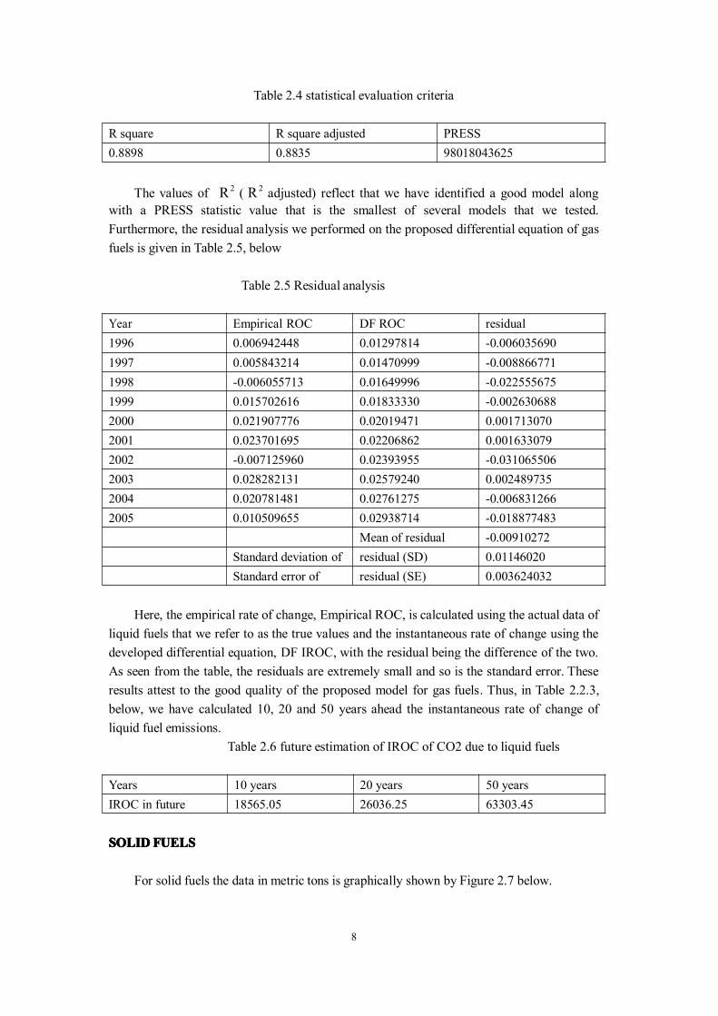
The IROC of liquid fuels as a function of time is given analytically by

. (2.8)7 4 2( ( )) 4.902 10 4.926 10 12.378d L t t tdt

= × − × × + ×

A graphical display of expression 2.8 is given by Figure 2.6

Figure 2.6 IROC of CO2 due to liquid fuels

The calculated values for the liquid fuel model for ( adjusted) and PRESS2R 2Rstatistic are given by Table 2.4, below

8

Table 2.4 statistical evaluation criteria

The values of ( adjusted) reflect that we have identified a good model along2R 2Rwith a PRESS statistic value that is the smallest of several models that we tested.Furthermore, the residual analysis we performed on the proposed differential equation of gasfuels is given in Table 2.5, below

Table 2.5 Residual analysis

Here, the empirical rate of change, Empirical ROC, is calculated using the actual data ofliquid fuels that we refer to as the true values and the instantaneous rate of change using thedeveloped differential equation, DF IROC, with the residual being the difference of the two.As seen from the table, the residuals are extremely small and so is the standard error. Theseresults attest to the good quality of the proposed model for gas fuels. Thus, in Table 2.2.3,below, we have calculated 10, 20 and 50 years ahead the instantaneous rate of change ofliquid fuel emissions.

Table 2.6 future estimation of IROC of CO2 due to liquid fuels

SOLIDSOLIDSOLIDSOLIDFUELSFUELSFUELSFUELS

For solid fuels the data in metric tons is graphically shown by Figure 2.7 below.

R square R square adjusted PRESS0.8898 0.8835 98018043625

Year Empirical ROC DF ROC residual1996 0.006942448 0.01297814 -0.0060356901997 0.005843214 0.01470999 -0.0088667711998 -0.006055713 0.01649996 -0.0225556751999 0.015702616 0.01833330 -0.0026306882000 0.021907776 0.02019471 0.0017130702001 0.023701695 0.02206862 0.0016330792002 -0.007125960 0.02393955 -0.0310655062003 0.028282131 0.02579240 0.0024897352004 0.020781481 0.02761275 -0.0068312662005 0.010509655 0.02938714 -0.018877483

Mean of residual -0.00910272Standard deviation of residual (SD) 0.01146020Standard error of residual (SE) 0.003624032

Years 10 years 20 years 50 yearsIROC in future 18565.05 26036.25 63303.45

9

1950 1960 1970 1980 1990 2000

2500

0035

0000

4500

0055

0000

Year

Sol

id F

uels

Figure 2.7 CO2 due to solid fuels from 1950 to 2005

The differential equation for solid fuels is given by

. (2.9)' 8 5 2( ) ( ) 4171.716 10 4.2818 10 109.9S t S t t t+ = × − × × + ×

The solution of 2.9 is given by

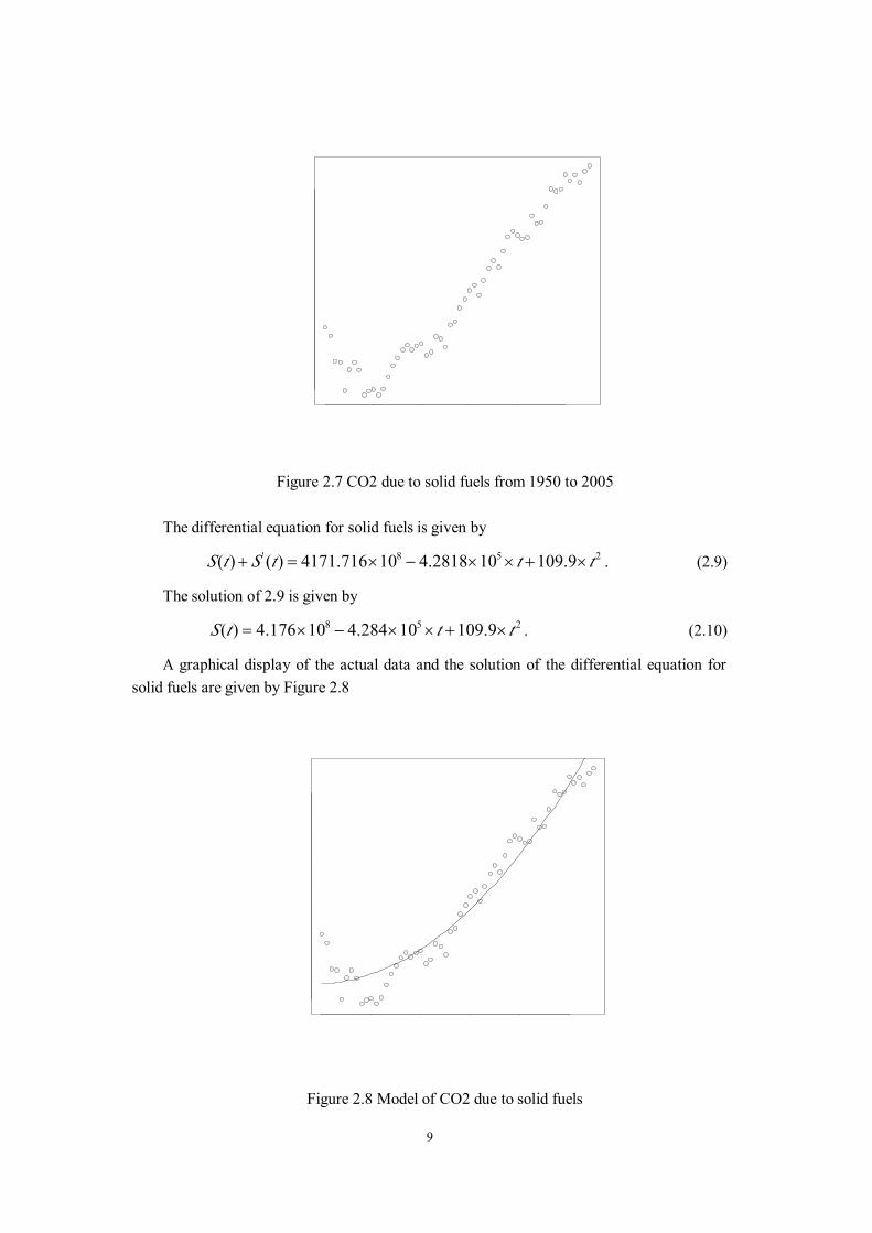
. (2.10)8 5 2( ) 4.176 10 4.284 10 109.9S t t t= × − × × + ×

A graphical display of the actual data and the solution of the differential equation forsolid fuels are given by Figure 2.8

1950 1960 1970 1980 1990 2000

2500

0035

0000

4500

0055

0000

Year

Solid

Fue

ls

Figure 2.8 Model of CO2 due to solid fuels

10

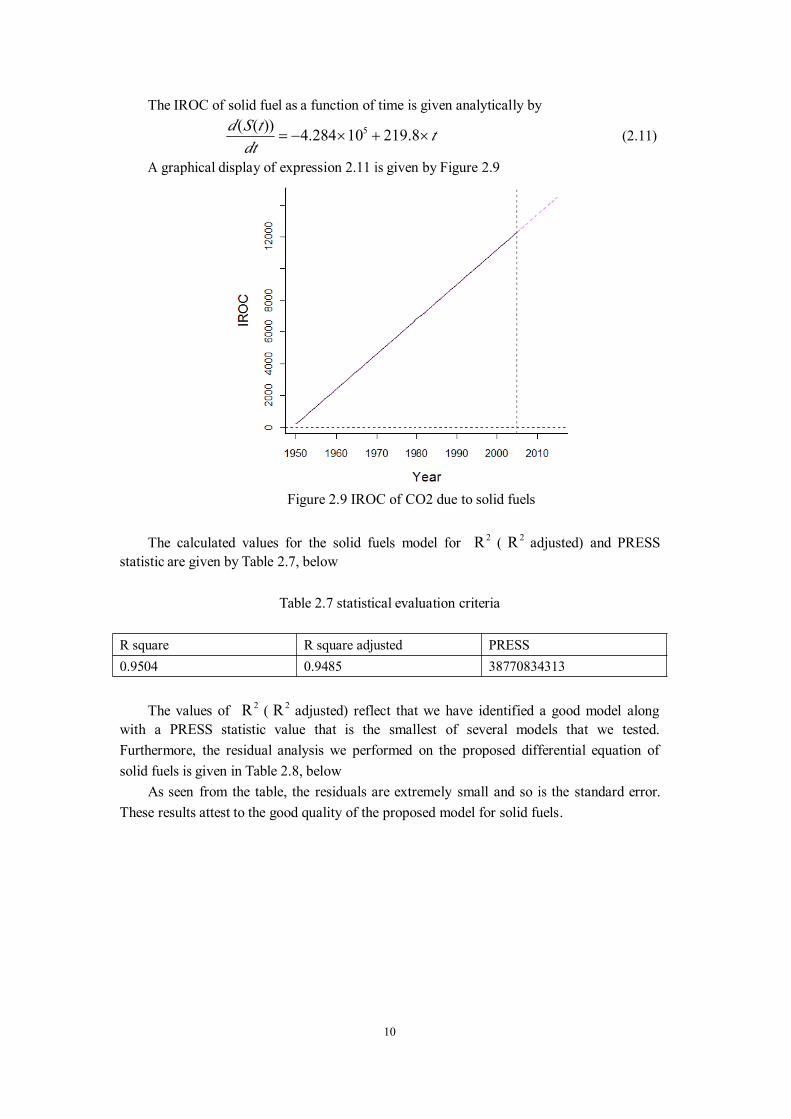
The IROC of solid fuel as a function of time is given analytically by

(2.11)5( ( )) 4.284 10 219.8d S t tdt

= − × + ×

A graphical display of expression 2.11 is given by Figure 2.9

Figure 2.9 IROC of CO2 due to solid fuels

The calculated values for the solid fuels model for ( adjusted) and PRESS2R 2Rstatistic are given by Table 2.7, below

Table 2.7 statistical evaluation criteria

The values of ( adjusted) reflect that we have identified a good model along2R 2Rwith a PRESS statistic value that is the smallest of several models that we tested.Furthermore, the residual analysis we performed on the proposed differential equation ofsolid fuels is given in Table 2.8, below

As seen from the table, the residuals are extremely small and so is the standard error.These results attest to the good quality of the proposed model for solid fuels.

R square R square adjusted PRESS0.9504 0.9485 38770834313

11

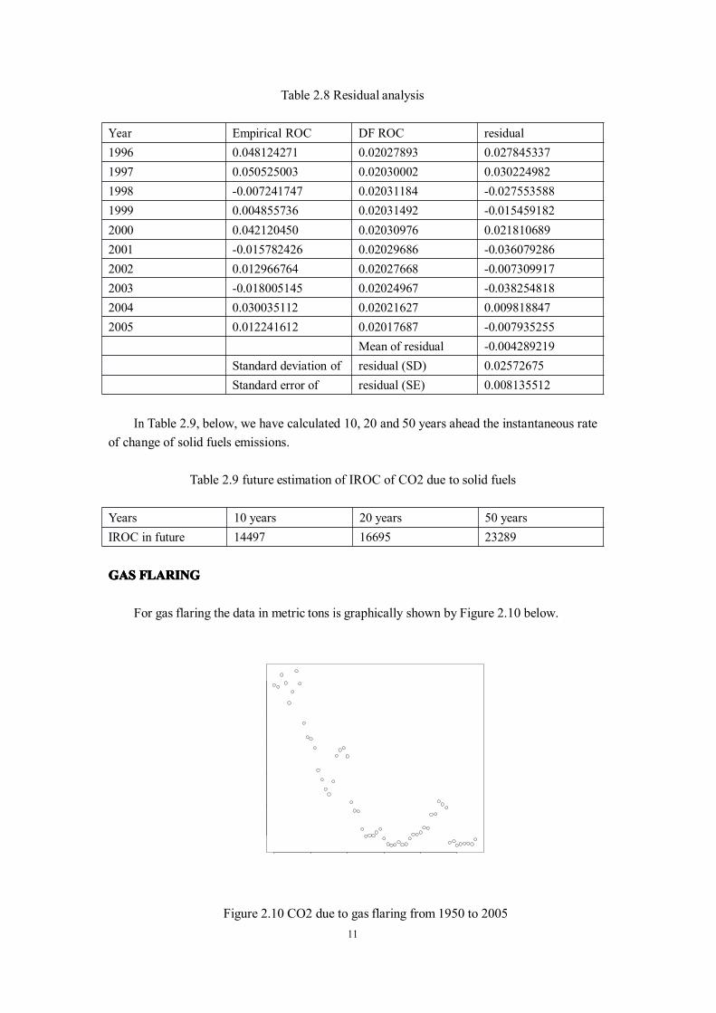
Table 2.8 Residual analysis

In Table 2.9, below, we have calculated 10, 20 and 50 years ahead the instantaneous rateof change of solid fuels emissions.

Table 2.9 future estimation of IROC of CO2 due to solid fuels

GASGASGASGAS FLARINGFLARINGFLARINGFLARING

For gas flaring the data in metric tons is graphically shown by Figure 2.10 below.

1950 1960 1970 1980 1990 2000

2000

4000

6000

8000

1000

012

000

Year

Gas

Fla

ring

Figure 2.10 CO2 due to gas flaring from 1950 to 2005

Year Empirical ROC DF ROC residual1996 0.048124271 0.02027893 0.0278453371997 0.050525003 0.02030002 0.0302249821998 -0.007241747 0.02031184 -0.0275535881999 0.004855736 0.02031492 -0.0154591822000 0.042120450 0.02030976 0.0218106892001 -0.015782426 0.02029686 -0.0360792862002 0.012966764 0.02027668 -0.0073099172003 -0.018005145 0.02024967 -0.0382548182004 0.030035112 0.02021627 0.0098188472005 0.012241612 0.02017687 -0.007935255

Mean of residual -0.004289219Standard deviation of residual (SD) 0.02572675Standard error of residual (SE) 0.008135512

Years 10 years 20 years 50 yearsIROC in future 14497 16695 23289

12

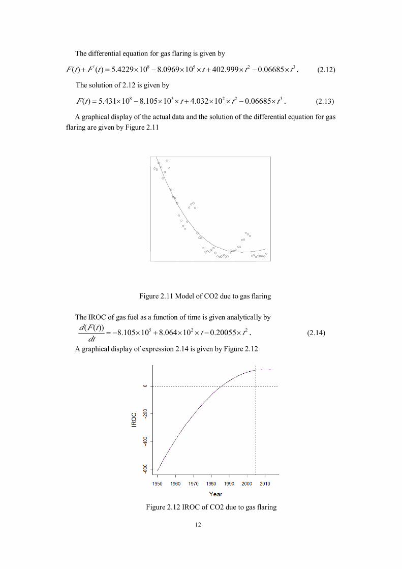
The differential equation for gas flaring is given by

. (2.12)' 8 5 2 3( ) ( ) 5.4229 10 8.0969 10 402.999 0.06685F t F t t t t+ = × − × × + × − ×

The solution of 2.12 is given by

. (2.13)8 5 2 2 3( ) 5.431 10 8.105 10 4.032 10 0.06685F t t t t= × − × × + × × − ×

A graphical display of the actual data and the solution of the differential equation for gasflaring are given by Figure 2.11

1950 1960 1970 1980 1990 2000

2000

4000

6000

8000

1000

012

000

Year

Gas

Fla

ring

Figure 2.11 Model of CO2 due to gas flaring

The IROC of gas fuel as a function of time is given analytically by

. (2.14)5 2 2( ( )) 8.105 10 8.064 10 0.20055d F t t tdt

= − × + × × − ×

A graphical display of expression 2.14 is given by Figure 2.12

Figure 2.12 IROC of CO2 due to gas flaring

13

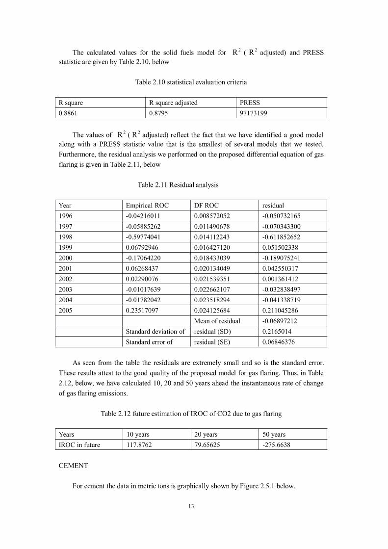
The calculated values for the solid fuels model for ( adjusted) and PRESS2R 2Rstatistic are given by Table 2.10, below

Table 2.10 statistical evaluation criteria

The values of ( adjusted) reflect the fact that we have identified a good model2R 2Ralong with a PRESS statistic value that is the smallest of several models that we tested.Furthermore, the residual analysis we performed on the proposed differential equation of gasflaring is given in Table 2.11, below

Table 2.11 Residual analysis

As seen from the table the residuals are extremely small and so is the standard error.These results attest to the good quality of the proposed model for gas flaring. Thus, in Table2.12, below, we have calculated 10, 20 and 50 years ahead the instantaneous rate of changeof gas flaring emissions.

Table 2.12 future estimation of IROC of CO2 due to gas flaring

CEMENT

For cement the data in metric tons is graphically shown by Figure 2.5.1 below.

R square R square adjusted PRESS0.8861 0.8795 97173199

Year Empirical ROC DF ROC residual1996 -0.04216011 0.008572052 -0.0507321651997 -0.05885262 0.011490678 -0.0703433001998 -0.59774041 0.014112243 -0.6118526521999 0.06792946 0.016427120 0.0515023382000 -0.17064220 0.018433039 -0.1890752412001 0.06268437 0.020134049 0.0425503172002 0.02290076 0.021539351 0.0013614122003 -0.01017639 0.022662107 -0.0328384972004 -0.01782042 0.023518294 -0.0413387192005 0.23517097 0.024125684 0.211045286

Mean of residual -0.06897212Standard deviation of residual (SD) 0.2165014Standard error of residual (SE) 0.06846376

Years 10 years 20 years 50 yearsIROC in future 117.8762 79.65625 -275.6638

14

1950 1960 1970 1980 1990 2000

6000

8000

1000

012

000

1400

0

Year

Cem

ent

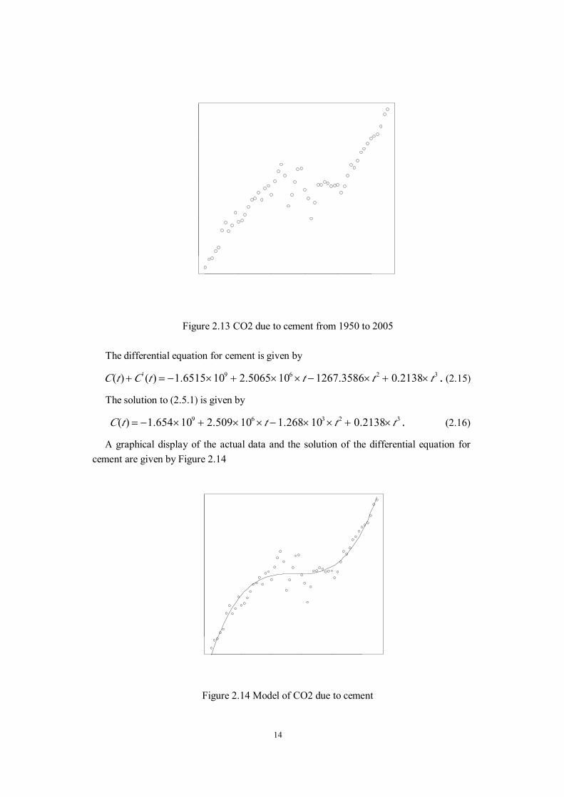
Figure 2.13 CO2 due to cement from 1950 to 2005

The differential equation for cement is given by

. (2.15)' 9 6 2 3( ) ( ) 1.6515 10 2.5065 10 1267.3586 0.2138C t C t t t t+ = − × + × × − × + ×

The solution to (2.5.1) is given by

. (2.16)9 6 3 2 3( ) 1.654 10 2.509 10 1.268 10 0.2138C t t t t= − × + × × − × × + ×

A graphical display of the actual data and the solution of the differential equation forcement are given by Figure 2.14

1950 1960 1970 1980 1990 2000

6000

8000

1000

012

000

1400

0

Year

Cem

ent

Figure 2.14 Model of CO2 due to cement

15

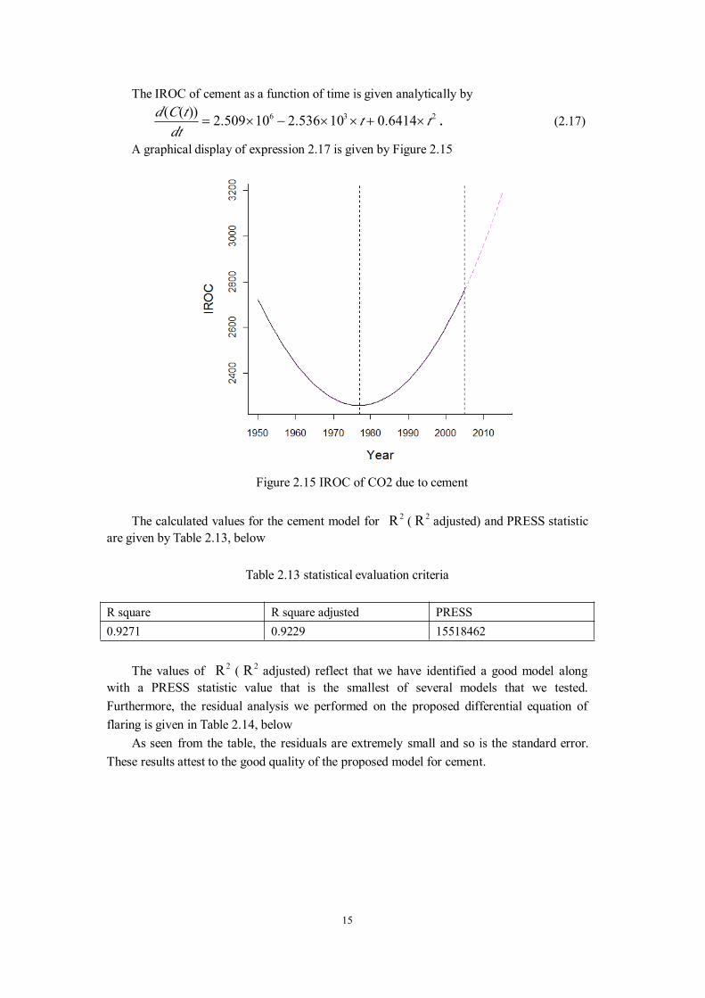
The IROC of cement as a function of time is given analytically by

. (2.17)6 3 2( ( )) 2.509 10 2.536 10 0.6414d C t t tdt

= × − × × + ×

A graphical display of expression 2.17 is given by Figure 2.15

Figure 2.15 IROC of CO2 due to cement

The calculated values for the cement model for ( adjusted) and PRESS statistic2R 2Rare given by Table 2.13, below

Table 2.13 statistical evaluation criteria

The values of ( adjusted) reflect that we have identified a good model along2R 2Rwith a PRESS statistic value that is the smallest of several models that we tested.Furthermore, the residual analysis we performed on the proposed differential equation offlaring is given in Table 2.14, below

As seen from the table, the residuals are extremely small and so is the standard error.These results attest to the good quality of the proposed model for cement.

R square R square adjusted PRESS0.9271 0.9229 15518462

16

Table 2.14 Residual analysis

Thus, in Table 2.15, below, we have calculated 10, 20 and 50 years ahead theinstantaneous rate of change of cement emissions.

Table 2.15 future estimation of IROC of CO2 due to cement

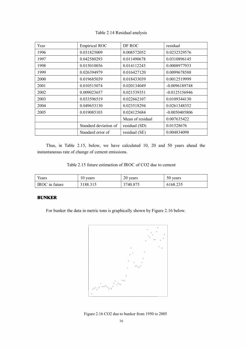
BUNKERBUNKERBUNKERBUNKER

For bunker the data in metric tons is graphically shown by Figure 2.16 below.

1950 1960 1970 1980 1990 2000

1000

015

000

2000

025

000

3000

035

000

4000

0

Year

Bunk

er

Figure 2.16 CO2 due to bunker from 1950 to 2005

Year Empirical ROC DF ROC residual1996 0.031825009 0.008572052 0.02325295761997 0.042580293 0.011490678 0.03108961451998 0.015010036 0.014112243 0.00089779331999 0.026394979 0.016427120 0.00996785882000 0.019685039 0.018433039 0.00125199992001 0.010515074 0.020134049 -0.00961897482002 0.009023657 0.021539351 -0.01251569462003 0.033596519 0.022662107 0.01093441302004 0.049653130 0.023518294 0.02613483522005 0.019085103 0.024125684 -0.0050405806

Mean of residual 0.007635422Standard deviation of residual (SD) 0.01528676Standard error of residual (SE) 0.004834098

Years 10 years 20 years 50 yearsIROC in future 3188.315 3740.875 6168.235

17

The differential equation for bunker is given by

. (2.18)' 9 6 2 3( ) ( ) 3.8941 10 5.9 10 2950.4949 .5017B t B t t t t+ = × − × × − × − ×

The solution to (2.18) is given by

. (2.19)9 6 3 2 3( ) 3.9 10 -5.906 10 2.98 10 -0.5017B t t t t= × × × + × × ×

A graphical display of the actual data and the solution of the differential equation forbunker are given by Figure 2.17

1950 1960 1970 1980 1990 2000

1000

015

000

2000

025

000

3000

035

000

4000

0

Year

Bun

ker

Figure 2.6.2 Model of CO2 due to bunker

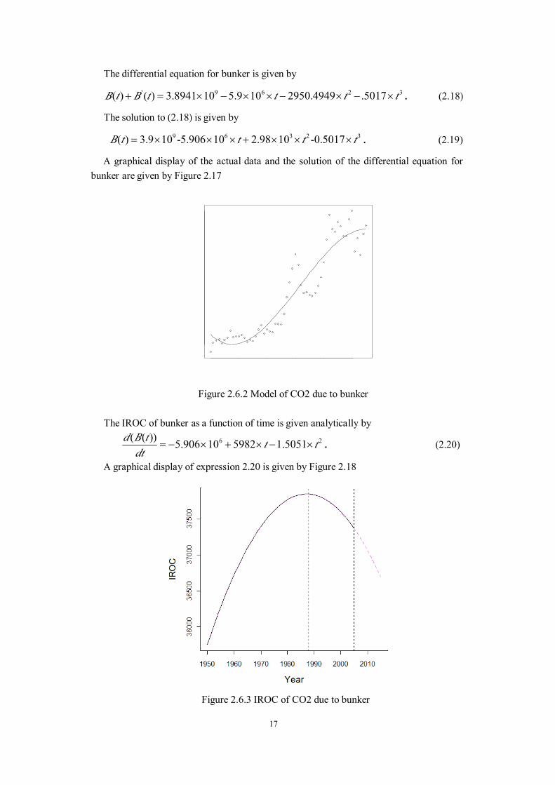
The IROC of bunker as a function of time is given analytically by

. (2.20)6 2( ( )) 5.906 10 5982 1.5051d B t t tdt

= − × + × − ×

A graphical display of expression 2.20 is given by Figure 2.18

Figure 2.6.3 IROC of CO2 due to bunker

18

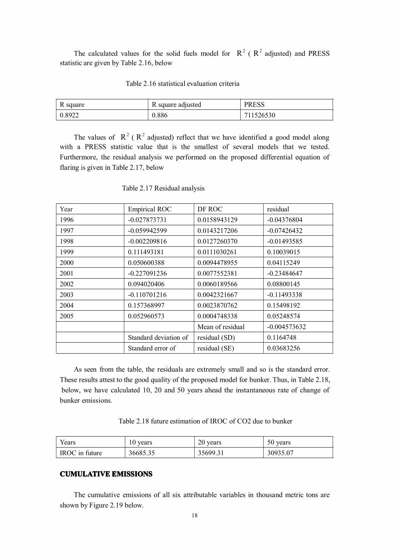
The calculated values for the solid fuels model for ( adjusted) and PRESS2R 2Rstatistic are given by Table 2.16, below

Table 2.16 statistical evaluation criteria

The values of ( adjusted) reflect that we have identified a good model along2R 2Rwith a PRESS statistic value that is the smallest of several models that we tested.Furthermore, the residual analysis we performed on the proposed differential equation offlaring is given in Table 2.17, below

Table 2.17 Residual analysis

As seen from the table, the residuals are extremely small and so is the standard error.These results attest to the good quality of the proposed model for bunker. Thus, in Table 2.18,below, we have calculated 10, 20 and 50 years ahead the instantaneous rate of change ofbunker emissions.

Table 2.18 future estimation of IROC of CO2 due to bunker

CUMULATIVECUMULATIVECUMULATIVECUMULATIVEEMISSIONSEMISSIONSEMISSIONSEMISSIONS

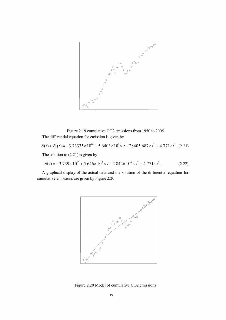
The cumulative emissions of all six attributable variables in thousand metric tons areshown by Figure 2.19 below.

R square R square adjusted PRESS0.8922 0.886 711526530

Year Empirical ROC DF ROC residual1996 -0.027873731 0.0158943129 -0.043768041997 -0.059942599 0.0143217206 -0.074264321998 -0.002209816 0.0127260370 -0.014935851999 0.111493181 0.0111030261 0.100390152000 0.050600388 0.0094478955 0.041152492001 -0.227091236 0.0077552381 -0.234846472002 0.094020406 0.0060189566 0.088001452003 -0.110701216 0.0042321667 -0.114933382004 0.157368997 0.0023870762 0.154981922005 0.052960573 0.0004748338 0.05248574

Mean of residual -0.004573632Standard deviation of residual (SD) 0.1164748Standard error of residual (SE) 0.03683256

Years 10 years 20 years 50 yearsIROC in future 36685.35 35699.31 30935.07

19

1950 1960 1970 1980 1990 2000

8000

0010

0000

012

0000

014

0000

016

0000

0

Year

cum

ulat

ive

emis

sion

s

Figure 2.19 cumulative CO2 emissions from 1950 to 2005The differential equation for emission is given by

. (2.21)' 10 7 2 3( ) ( ) 3.73335 10 5.6403 10 28405.687 4.771E t E t t t t+ = − × + × × − × + ×

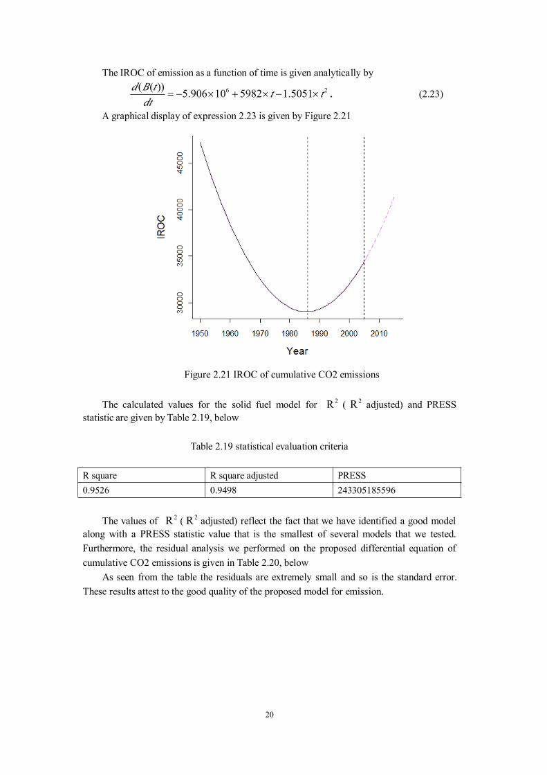
The solution to (2.21) is given by

. (2.22)10 7 4 2 3( ) 3.739 10 5.646 10 2.842 10 4.771E t t t t= − × + × × − × × + ×

A graphical display of the actual data and the solution of the differential equation forcumulative emissions are given by Figure 2.20

1950 1960 1970 1980 1990 2000

8000

0010

0000

012

0000

014

0000

016

0000

0

Year

cum

ulat

ive

emis

sion

s

Figure 2.20 Model of cumulative CO2 emissions

20

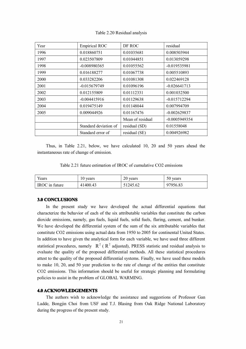
The IROC of emission as a function of time is given analytically by

. (2.23)6 2( ( )) 5.906 10 5982 1.5051d B t t tdt

= − × + × − ×

A graphical display of expression 2.23 is given by Figure 2.21

Figure 2.21 IROC of cumulative CO2 emissions

The calculated values for the solid fuel model for ( adjusted) and PRESS2R 2Rstatistic are given by Table 2.19, below

Table 2.19 statistical evaluation criteria

The values of ( adjusted) reflect the fact that we have identified a good model2R 2Ralong with a PRESS statistic value that is the smallest of several models that we tested.Furthermore, the residual analysis we performed on the proposed differential equation ofcumulative CO2 emissions is given in Table 2.20, below

As seen from the table the residuals are extremely small and so is the standard error.These results attest to the good quality of the proposed model for emission.

R square R square adjusted PRESS0.9526 0.9498 243305185596

21

Table 2.20 Residual analysis

Thus, in Table 2.21, below, we have calculated 10, 20 and 50 years ahead theinstantaneous rate of change of emission.

Table 2.21 future estimation of IROC of cumulative CO2 emissions

3.03.03.03.0 CONCLUSIONSCONCLUSIONSCONCLUSIONSCONCLUSIONSIn the present study we have developed the actual differential equations that

characterize the behavior of each of the six attributable variables that constitute the carbondioxide emissions, namely, gas fuels, liquid fuels, solid fuels, flaring, cement, and bunker.We have developed the differential system of the sum of the six attributable variables thatconstitute CO2 emissions using actual data from 1950 to 2005 for continental United States.In addition to have given the analytical form for each variable, we have used three differentstatistical procedures, namely ( adjusted), PRESS statistic and residual analysis to2R 2Revaluate the quality of the proposed differential methods. All these statistical proceduresattest to the quality of the proposed differential systems. Finally, we have used these modelsto make 10, 20, and 50 year prediction to the rate of change of the entities that constituteCO2 emissions. This information should be useful for strategic planning and formulatingpolicies to assist in the problem of GLOBAL WARMING.

4.04.04.04.0ACKNOWLEDGEMENTSACKNOWLEDGEMENTSACKNOWLEDGEMENTSACKNOWLEDGEMENTSThe authors wish to acknowledge the assistance and suggestions of Professor Gan

Ladde, Bongjin Choi from USF and T.J. Blasing from Oak Ridge National Laboratoryduring the progress of the present study.

Year Empirical ROC DF ROC residual1996 0.018860751 0.01035681 0.0085039441997 0.023507809 0.01044851 0.0130592981998 -0.008980365 0.01055562 -0.0195359811999 0.016188277 0.01067738 0.0055108932000 0.033282206 0.01081308 0.0224691282001 -0.015679749 0.01096196 -0.0266417132002 0.012155809 0.01112331 0.0010325002003 -0.004415916 0.01129638 -0.0157122942004 0.019475149 0.01148044 0.0079947092005 0.009044926 0.01167476 -0.002629837

Mean of residual -0.0005949354Standard deviation of residual (SD) 0.01558048Standard error of residual (SE) 0.004926982

Years 10 years 20 years 50 yearsIROC in future 41400.43 51245.62 97956.83

22

Reference:Reference:Reference:Reference:

1. Adrien C. Finzi and William H. Schlesinger, Aug., 2003. Ecosystems, Vol. 6, No. 5,pp. 444-456

2. Blasing, T.J. C.T. Broniak and G. Marland, 2005. The annual cycle of fossil-fuelscarbon dioxide emissions in the United States. Tellus, 57B57B57B57B, 107-115.

3. Blasing, T.J. and K. Hand. 2007. Monthly carbon emissions from natural-gas flaringand cement manufacture in the United States. Tellus 59B,59B,59B,59B, 15-21.

4. Blasing, T.J. Christine Broniak and G. Marland, 2005. State-by state carbon dioxideemissions from fossil fuels use in the United States 1960-2000. Mitigation andAdaptation Strategies for Global Change 10,10,10,10, 659-674.

5. BovasAbraham and Johannes Ledolter, 2006. Introduction to regression modeling.6. Chris P. Tsokos, June, 2007. The 5th International Conference on Dynamic Systems

and Applications, ICDSA5, Title-“Statistical Modeling of Global Warming”, IFNA,Atlanta, Georgia.

7. Chris P. Tsokos, 2008. GVP Institute of Advanced Studies, Title-“Global Warming”,Visakha patnam, India.

8. Chris P. Tsokos, 2008. GVP Institute of Advanced Studies, Title-“Carbon Dioxide inthe Atmosphere”, Visakha patnam, India.

9. Chris P. Tsokos, July, 2008. The 6th International Congress of IFNA, Title-“GlobalWarming”, IFNA, Orlando, Florida.

10. Gregory J. Retallack, Apr. 15, 2002. Philosophical Transactions: Mathematical,Physical and Engineering Sciences, Vol. 360, No. 1793, Understanding ClimateChange: Proxies, Chronology and Ocean-Atmosphere Interactions, pp. 659-673

11. Hansen, J. and Takahashi. T, 1984. Climate processes and Climate Sensitivity.Geophysical Monograph 39.American Geophysical Union, Washington DC.

12. James A. Bunce, Nov., 2001. International Journal of Plant Sciences, Vol. 162, No.6, pp. 1261-1266

13. Jason G. Hamilton, Evan H. DeLucia, Kate George, Shawna L. Naidu, Adrien C.Finzi and William H. Schlesinger, Apr., 2002. Oecologia, Vol. 131, No. 2, pp. 250-260

14. Kyaw Tha Paw U, Matthias Falk, Thomas H. Suchanek, Susan L. Ustin, JiquanChen, Young-San Park, William E. Winner, Sean C. Thomas, Theodore C. Hsiao,Roger H. Shaw, Thomas S. King, R. David Pyles, Matt Schroeder and Anthony A.Matista, Aug., 2004. Ecosystems, Vol. 7, No. 5, pp. 513-524

15. Laurie J. Osher, Pamela A. Matson and Ronald Amundson, Sep., 2003.Biogeochemistry, Vol. 65, No. 2, pp. 213-232

16. Lashof, D, 1989. The dynamic greenhouse: feedback processes that may influencefuture concentrations of atmospheric trace gases and climatic change. Climatic

23

Change 14, 213-24217. Marland, G., R. Andres, T.J. Blasing, T.A. Boden, C.T. Broniak, J.S. Gregg, L.M.

Losey, and K. Treanton, 2007. Energy, Industry, andWaste Management Activities:An Introduction to CO2 Emissions from Fossil Fuels. pp 57-64 IN: First State of theCarbon Cycle Report (SOCCR): The North American Carbon Project andImplications for the Global Carbon Cycle., United States Climate Change ScienceProgram Synthesis andAssessment Product 2.2, National Oceanic andAtmosphericAdministration, National Climatic Data Center, Asheville, NC, USA. 242 pp.

18. Pieter P. Tans, Inez Y. Fung and Taro Takahashi, Mar. 23, 1990. Science, New Series,Vol. 247, No. 4949, pp. 1431-1438

19. R. D. Cess, G. L. Potter, J. P. Blanchet, G. J. Boer, S. J. Ghan, J. T. Kiehl, H. Le Treut,Z.-X. Li, X.-Z. Liang, J. F. B. Mitchell, J.-J. Morcrette, D. A. Randall, M. R. Riches,E. Roeckner, U. Schlese, A. Slingo, K. E. Taylor, W. M. Washington, R. T. Wetheraldand I. Yagai, Aug. 4, 1989. Science, New Series, Vol. 245, No. 4917, pp. 513-516

20. Thomas J. Goreau, 1990. Balancing Atmospheric Carbon Dioxid. Ambio, Vol. 19,No. 5 (Aug., 1990), pp. 230-236

21. V. Ramanathan, Apr. 15, 1988. The Greenhouse Theory of Climate Change: A Test by

an Inadvertent Global Experiment, Science, New Series, Vol. 240, No. 4850, pp. 293-299

22. Wolfgang Cramer, Alberte Bondeau, Sibyll Schaphoff, Wolfgang Lucht, BenjaminSmith and Stephen Sitch, Mar. 29, 2004. Philosophical Transactions: BiologicalSciences, Vol. 359, No. 1443, Tropical Forests and Global Atmospheric Change, pp.331-343