Modeling changes to the historic Lower Columbia River

Drew Mahedy

Lumas Helaire

Stefan Talke

David Jay

May 30, 2014

Modeling changes to the historic Lower

Columbia River Estuary using Delft3D

Comparison: Historic and Modern LCRE

Historic 19th century Digital elevation model for

the Columbia exists (digitized by Jen Burke et

al. at U. Washington)

US Coastal

Survey, 1868

Two Delft3D hydrodynamic models

have been developed– a modern and a

Historic D3D Model

• 5 sub-domains

• Shelf/estuary, estuary, lower, upper

• ~50-200 m grid resolution

• More refined in the estuary and upstream

near the Willamette River

• Tidal boundary condition

• Along the shelf

• M2, N2, S2, K1, P1, O1

• Discharge boundary conditions

• The Dalles, 1878 USGS flow (Bonneville)

• Oregon City, 1878 USGS flow (Morrison

Bridge)

Historic Columbia River model

domain

Sample HCR model depths in the

estuary domain showing domain

decomposition boundaries

Two Delft3D hydrodynamic models have

been developed:

1. 21st century model based on 2005

bathymetry (modified from USGS model

of Gelfenbaum& Elias (2012)

2. 19th century model based on Burke

(2002) digitized bathymetry

(bathymetric surveys from 1868-1900)

1877 Columbia River Tide Data

Temporal Coverage for calibration

Long Data set from 1853-1876 available at Astoria

Vancouver, WA September 1877

Data from US National Archives

Tide Changes: Preliminary Results

Next: Tide Variations

Mean Tidal Range

has increased

by half a foot





Astoria

SF Bay Friction on a tide wave is larger when:

(1) Water is shallow (e.g. tidal flats)

(2) Bathymetry (e.g., dunes) is pronounced

(3) River Flow is larger

(4) Internal shear larger

Friction extracts energy from tidal

constituents and puts it into higher

‘harmonics’, or ‘overtides’. For example,

the twice daily M2 lunar tide produces an

M4 (4 times daily) overtide.

Both SF and especially Astoria were

much more ‘frictional’ in the past.

Spectral energy at the 4 cpd frequency

much larger in the 19th century

One way to tease apart local and basin-scale changes is to look at

the locally produced, non-linear shallow-water overtides

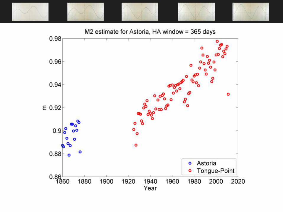
Overtide variation

M4 Astoria M4 overtide in Astoria decreased from 2

cm to 5 mm during the 20th century

Nearby Ocean stations show little

variation

Why???

Local effects: construction of the

Columbia Bar, dredging, deepening, etc.

M4 Crescent

City, CA

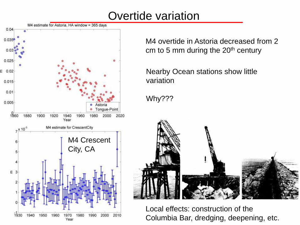
Deepening of the Elbe River, Germany since 1900

One hypothesis

Local, anthropogenic effects such as

channel deepening and streamlining

are in many cases a primary cause of

long-term change.

Depth driven by ship size

Schematic of

a convergent

estuary

Tidal heights become a balance between the

amplifying effects of convergence and the

damping by friction.

In many convergent estuaries, the first order

momentum balance is between the pressure

gradient and friction (e.g., Friedrichs & Aubrey,

1994):

Observation: Increasing depth has a similar

dynamical effect as decreasing drag coefficient

What do other studies suggest is important?

But tides in estuaries are complicated.

Factors important to tidal propagation and

overtide production include:

2. Resonance = 4LT ω/(gH)½

2

2

2

2

2

~XUC

HgS

dx

ds

UC

gHRi

d

o

d

x

3. Internal tidal asymmetry (Simpson #)

4. Other factors such as ratio of intertidal

flats/channel volume (Friedrichs and

Aubrey, 1988) and ratio of nonlinear to

local acceleration (Ianiello, 1979) can be

important.

1. Nonlinear tidal asymmetry (production of

overtides) is controlled by the ratio of

acceleration/friction:

= Ianiello # = ωH2/Km (Ianniello, 1977; this is the inverse Strouhal

number of Burchard 2009) Effects of

increasing

depth/decreasing

friction have

same dynamical

effect

Similarly , diurnal

and semidiurnal

constituents

ought to have a

different reaction

to deepening

Analyze old data…

Observations in Columbia River

1. M2 increased in estuary (km 0-

30) between 1877 and 1941

2. M2 and S2 increased in the tidal

river between 1941 and the present

3. Overtides decreased in estuary

between 1877 and 1941

4. The ‘overtide’ maximum shifted

upstream

The changed constituents produce

altered tidal behavior

1. The system is less frictional, as

observed in the M4/M22 ratio

3. The K1 behavior is mixed. More

analysis needed

2. Spring-Neap ratio has increased

(As system becomes less frictional,

S2 becomes less damped by M2;

see e.g. Godin, 1997)

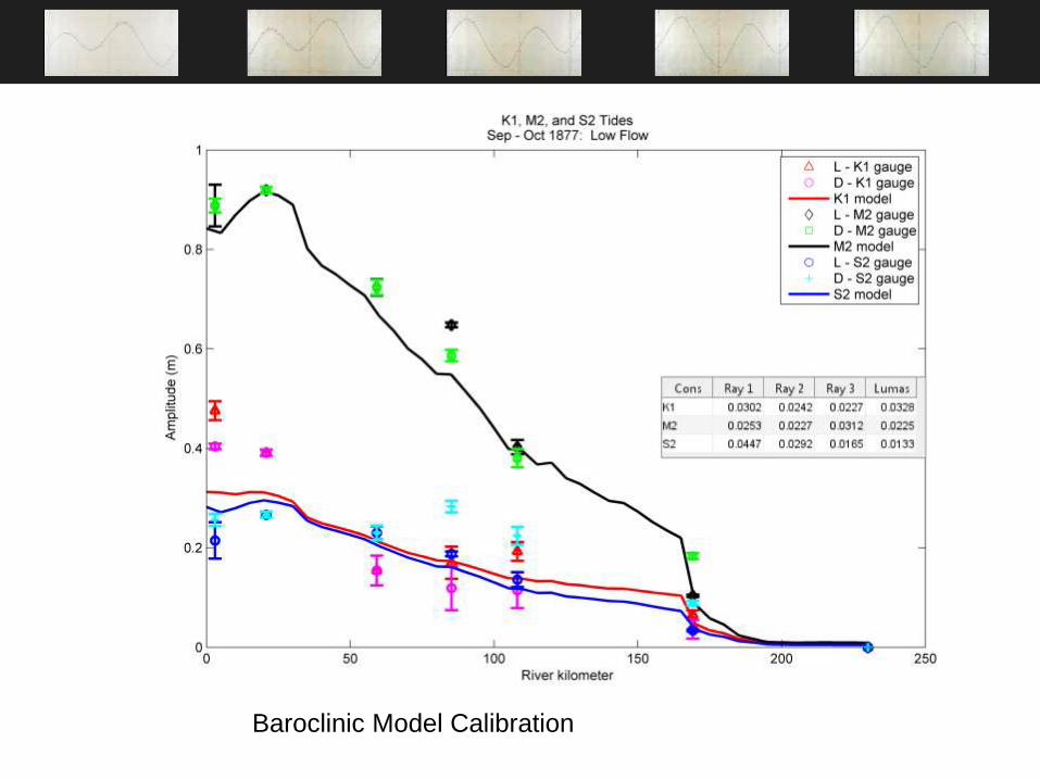
Model: A Delft3D model is

being made to determine the

causes of change.

The model is currently

calibrated to tide data and does

as well as the modern model.

Note: The M2 maximum has

moved upstream from Astoria

towards Astoria Tongue Point/

Cathlamet Bay.

Hence: The Tongue Point tide

data has actually changed

*more* than the prevous

graphs suggested.

Barotropic Model Run…

Model: A Delft3D model is

being made to determine the

causes of change.

The model is currently

calibrated to tide data and does

as well as the modern model.

Baroclinic Model Calibration

Preliminary Results

1. Increasing depth produces

greater constituent amplitudes

2. Overtide maximum is moved

upstream

3. M4/M22 ratio forced

downwards everywhere

4. Spring Neap ratio increased

5. System more diurnal, but not

everywhere.

Results from an idealized version of

the 19th cnetury model:

Spring Tide inundation

Youngs Bay, Modern Inundation Youngs Bay, Historic Inundation

Spring Tide inundation

Cathlamet Bay, Modern Inundation Youngs Bay, Historic Inundation

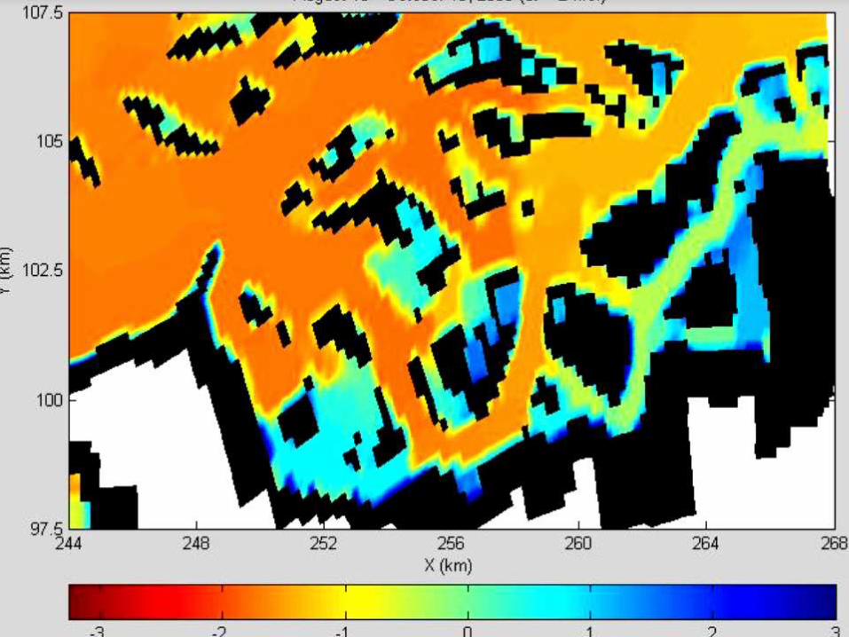
Preliminary Results

3 Videos:

1. Water levels

2. Salinity

3. Bed stress

Baker Bay

Next Steps

1. Determine how much tides have affected wetland habitat, and where

2. Determine the primary reasons for altered long-wave behavior

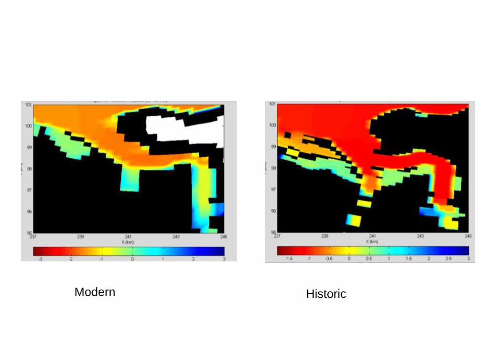
Modern Historic

Future Steps:

--Change bathymetry and see what happens.

-- Simulate extreme events (e.g., 1876 flood).

What would that flood look like today,

under both ‘virgin’ flow and regulated scenarios?

--Water Temperature and Salinity Intrusion

Although we do not have salinity data, we

have a treasure trove of temperature data,

including top/bottom from Ft. Canby, 1883-1888.

Point would be: How has the

temperature/salinity climate of wetlands changed

over time?

Finally: What lessons are there for

climate change?

Water Temperature much

larger than 1850s…

Gradient between upriver

and estuary switched (river

used to be colder)

Dotted-Vancouver;

Solid: Astoria

Final thoughts (some things to think about) An incomplete list of long-term changes to estuary boundary conditions includes: --tides --sea level --Meteorological changes (e.g., NAO index) --river flow --sediment input --nutrient input --bathymetry --habitat --???? Changes may be quite obvious, or be subtle and occur over a long time (e.g., changes to Columbia tidal components). Changes often produce a non-linear cascade of events. Everything affects everything. Moreover, both natural and anthropogenic change are often wrapped together. Anthropogenic effects include --

Tide data are the oldest oceanographic data sets that can address

these issues Recovery of these data is important


Approximate Maximum Tide amplitude, 19th century: M2 +S2 +N2 + O1 +K1

1.92m

Approximate Maximum Tide amplitude, 21st century: M2 +S2 +N2 + O1 +K1

2.05m

Greater tidal range is as much as 1 foot larger now than in 19th century.

Impacts both the high and the low waters.

However, This needs to be considered within the spatial

variation of tides in the estuary.

(Maximum Difference of 3.84m between high and low tide)

(Maximum Difference of 4.1m between high and low tide)

Documents

Modeling changes to the historic Lower Columbia River