SANDIA REPORT

SAND2004-4096 Unlimited Release Printed September 2004 Modeling Coupled Blast/Structure Interaction with Zapotec, Benchmark Calculations for the Conventional Weapon Effects Backfill (CONWEB) Tests Greg C. Bessette Prepared by Sandia National Laboratories Albuquerque, New Mexico 87185 and Livermore, California 94550 Sandia is a multiprogram laboratory operated by Sandia Corporation, a Lockheed Martin Company, for the United States Department of Energy’s

National Nuclear Security Administration under Contract DE-AC04-94AL85000. Approved for public release; further dissemination unlimited.

Issued by Sandia National Laboratories, operated for the United States Department of Energy by Sandia Corporation.

NOTICE: This report was prepared as an account of work sponsored by an agency of the United States Government. Neither the United States Government, nor any agency thereof, nor any of their employees, nor any of their contractors, subcontractors, or their employees, make any warranty, express or implied, or assume any legal liability or responsibility for the accuracy, completeness, or usefulness of any information, apparatus, product, or process disclosed, or represent that its use would not infringe privately owned rights. Reference herein to any specific commercial product, process, or service by trade name, trademark, manufacturer, or otherwise, does not necessarily constitute or imply its endorsement, recommendation, or favoring by the United States Government, any agency thereof, or any of their contractors or subcontractors. The views and opinions expressed herein do not necessarily state or reflect those of the United States Government, any agency thereof, or any of their contractors. Printed in the United States of America. This report has been reproduced directly from the best available copy. Available to DOE and DOE contractors from

U.S. Department of Energy Office of Scientific and Technical Information P.O. Box 62 Oak Ridge, TN 37831 Telephone: (865)576-8401 Facsimile: (865)576-5728

E-Mail: reports@adonis.osti.govOnline ordering: http://www.osti.gov/bridge

Available to the public from

U.S. Department of Commerce National Technical Information Service 5285 Port Royal Rd Springfield, VA 22161 Telephone: (800)553-6847 Facsimile: (703)605-6900

E-Mail: orders@ntis.fedworld.govOnline order: http://www.ntis.gov/help/ordermethods.asp?loc=7-4-0#online

2

SAND2004-4096 Printed September 2004

Modeling Coupled Blast/Structure Interaction with Zapotec, Benchmark Calculations for the Conventional Weapon

Effects Backfill (CONWEB) Tests

Greg C. Bessette Computational Physics and Simulation Frameworks (9232)

Sandia National Laboratories P.O. Box 5800

Albuquerque, NM 87185-0820

Abstract Modeling the response of buried reinforced concrete structures subjected to close-in detonations of conventional high explosives poses a challenge for a number of reasons. Foremost, there is the potential for coupled interaction between the blast and structure. Coupling enters the problem whenever the structure deformation affects the stress state in the neighboring soil, which in turn, affects the loading on the structure. Additional challenges for numerical modeling include handling disparate degrees of material deformation encountered in the structure and surrounding soil, modeling the structure details (e.g., modeling the concrete with embedded reinforcement, jointed connections, etc.), providing adequate mesh resolution, and characterizing the soil response under blast loading. There are numerous numerical approaches for modeling this class of problem (e.g., coupled finite element/smooth particle hydrodynamics, arbitrary Lagrange-Eulerian methods, etc.). The focus of this work will be the use of a coupled Euler-Lagrange (CEL) solution approach. In particular, the development and application of a CEL capability within the Zapotec code is described. Zapotec links two production codes, CTH and Pronto3D. CTH, an Eulerian shock physics code, performs the Eulerian portion of the calculation, while Pronto3D, an explicit finite element code, performs the Lagrangian portion. The two codes are run concurrently with the appropriate portions of a problem solved on their respective computational domains. Zapotec handles the coupling between the two domains. The application of the CEL methodology within Zapotec for modeling coupled blast/structure interaction will be investigated by a series of benchmark calculations. These benchmarks rely on data from the Conventional Weapons Effects Backfill (CONWEB) test series. In these tests, a 15.4-lb pipe-encased C-4 charge was detonated in soil at a 5-foot standoff from a buried test structure. The test structure was composed of a reinforced concrete slab bolted to a reaction structure. Both the slab thickness and soil media were varied in the test series. The wealth of data obtained from these tests along with the variations in experimental setups provide ample opportunity to assess the robustness of the Zapotec CEL methodology.

3

Acknowledgements This work was carried out under a Sandia National Laboratories CSRF (Project/Task 7101/04.16), titled “Modeling Coupled Blast/Target Interaction to Evaluate Facility Response and Structural Collapse”. The author would like to thank James Baylot (ERDC) for providing experimental data for code benchmarking, as well as his insights into the experimental procedure and results; Marlin Kipp (9232) for his insights into modeling blast with CTH; and Marlin Kipp (9232) and Steve Attaway (9134) for their review of this report. The author would also like to acknowledge the many contributors to Zapotec’s development. The original Zapotec code was developed in the early 1990s by John Prentice of Quetzal Computational Associates. This version of Zapotec performed a serial coupling of the CTH and EPIC codes, and was largely focused on penetration applications. Zapotec evolved over the years with a number of Sandians involved in the development. To the authors knowledge, the Sandians involved were Paul Yarrington, Stewart Silling, Courtenay Vaughan, Ray Bell, Sue Goudy, Don Peterson, Richard Koteras, and Steve Attaway. The evolution of the code development has included developing a link with Pronto3D, developing a parallel implementation of the coupling algorithm, and expanding its capabilities to model a broader class of problems.

4

Contents Page Abstract 3 Acknowledgements 4 1.0 Introduction 7 2.0 General Description of the Zapotec Coupling Algorithm 8

3.0 CONWEB Test Description 12 3.1 Experimental Setup - Test 1 12

3.2 Experimental Setup - Test 2 16 3.3 Experimental Setup - Test 3 17

4.0 CONWEB Test 1 19 4.1 Problem Setup 19 4.2 Analysis Results 26 4.3 Zapotec Code Modifications and Updated Results 49 4.4 Summary 51 5.0 CONWEB Test 2 53 5.1 Problem Setup 53 5.2 Analysis Results 54 5.3 Summary 58 6.0 CONWEB Test 3 67 6.1 Problem Setup 67 6.2 Analysis Results 67 6.3 Summary 70 7.0 Concluding Remarks 80 8.0 References 82 Appendix A – Sample Input Files, CONWEB Test 1 85 Appendix B – Development of Material Fit for Reconstituted Clay 97 Appendix C – Development of Material Fit for Compacted Concrete Sand 107 Distribution 113

5

This Page Intentionally Left Blank

6

1.0 Introduction Modeling the response of buried reinforced concrete structures subjected to close-in detonations of conventional high explosives poses a challenge for a number of reasons. Foremost, there is the potential for coupled interaction between the blast and structure. Coupling enters the problem whenever the structure deformation affects the stress state in the neighboring soil, which in turn, affects the loading on the structure. For close-in detonations, coupled interaction is generally assured since the induced loading on the structure usually results in significant deformations and/or rigid body motion within the soil. Additional challenges for numerical modeling include handling disparate degrees of material deformation encountered in the structure and surrounding soil, modeling the structure details (e.g., modeling the concrete with embedded reinforcement, jointed connections, etc.), providing adequate mesh resolution, and characterizing the soil response under blast loading. There are numerous numerical approaches for modeling this class of problem (e.g., coupled finite element/smooth particle hydrodynamics, arbitrary Lagrange-Eulerian methods, etc.). The focus of this work will be the use of a coupled Euler-Lagrange (CEL) solution approach. This approach is advantageous as it allows flexibility in modeling different portions of the problem using either Eulerian or Lagrangian techniques. For example, the explosive and soil can be modeled as Eulerian as this approach readily handles the shock transmission and large material deformations involved; the reinforced concrete structure can be modeled using a Lagrangian finite element method, as this approach allows for detailed modeling of structure components and their response. In this report, the development and application of a CEL capability within the Zapotec code is described. Zapotec links two production codes, CTH and Pronto3D. CTH, an Eulerian shock physics code, performs the Eulerian portion of the calculation, while Pronto3D, an explicit finite element code, performs the Lagrangian portion. The two codes are run concurrently with the appropriate portions of a problem solved on their respective computational domains. Zapotec handles the coupling between the two domains. The application of the CEL methodology within Zapotec for modeling coupled blast/structure interaction will be investigated by a series of benchmark calculations. These benchmarks rely on data from the Conventional Weapons Effects Backfill (CONWEB) test series. In these tests, a 15.4-lb pipe-encased C-4 charge was detonated in soil at a 5-foot standoff from a buried test structure. The test structure was composed of a reinforced concrete slab bolted to a reaction structure. Both the slab thickness and soil media were varied in the test series. The wealth of data obtained from these tests along with the variations in experimental setups provide ample opportunity to assess the robustness of the Zapotec CEL methodology.

7

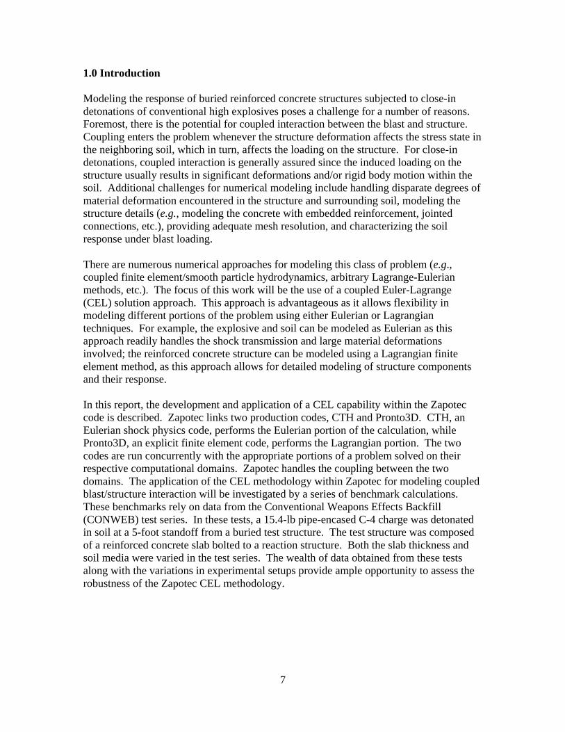
2.0 General Description of the Zapotec Coupling Algorithm Zapotec is a coupled Euler-Lagrange code that links the CTH and Pronto3D codes (Silling (2000), Bessette, et al. (2002, 2003, 2003a)). CTH, an Eulerian shock physics code, performs the Eulerian portion of the calculation, while Pronto3D, an explicit finite element code, performs the Lagrangian portion. The two codes are run concurrently with the appropriate portions of a problem solved on their respective computational domains. Zapotec handles the coupling between the two domains. Both CTH and Pronto3D are well documented (e.g., see McGlaun, et al. (1990), Hertel, et al. (1993), Bell, et al. (2000), Attaway, et al. (1998), Taylor and Flanagan (1989)) and the remaining discussion will focus on Zapotec. Zapotec controls both the time synchronization between CTH and Pronto3D as well as the interaction between materials on their respective computational domains. At a given time tn, Zapotec performs the coupled treatment between the Eulerian and Lagrangian materials in the problem. Once this treatment is complete, both CTH and Pronto3D are run independently over the next Zapotec time step (see Figure 2-1). In general, the Pronto3D stable time step will be smaller than that for CTH. When this occurs, Zapotec allows subcycling of Pronto3D for computational efficiency and accuracy. The subcycling continues until time tn+1 is reached, ensuring the two codes are synchronized.

Figure 2-1. Zapotec Time Synchronization

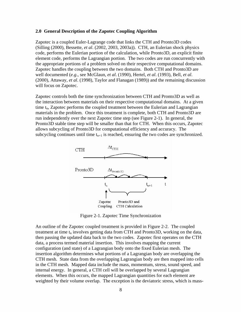
An outline of the Zapotec coupled treatment is provided in Figure 2-2. The coupled treatment at time tn involves getting data from CTH and Pronto3D, working on the data, then passing the updated data back to the two codes. Zapotec first operates on the CTH data, a process termed material insertion. This involves mapping the current configuration (and state) of a Lagrangian body onto the fixed Eulerian mesh. The insertion algorithm determines what portions of a Lagrangian body are overlapping the CTH mesh. State data from the overlapping Lagrangian body are then mapped into cells in the CTH mesh. Mapped data include the mass, momentum, stress, sound speed, and internal energy. In general, a CTH cell will be overlapped by several Lagrangian elements. When this occurs, the mapped Lagrangian quantities for each element are weighted by their volume overlap. The exception is the deviatoric stress, which is mass-

8

weighted. The weighted quantities are accumulated for all elements overlapping a cell, after which the intrinsic value is recovered for insertion. The inserted data are then passed back to CTH as a mesh update.

(1) Remove pre-existing Lagrangian material from the CTH mesh (2) Get updated Lagrangian data (3) Insert Lagrangian material into the CTH mesh (a) Compute volume overlaps (b) Map Lagrangian data – mass, momentum, stress, sound speed, internal energy (c) Pass updated mesh data back to CTH (4) Compute external forces on Lagrangian surface (a) Determine surface overlaps (b) Compute surface tractions based on Eulerian stress state (c) Compute normal force on element surface (element-centered force) (d) If friction, compute tangential force (e) Distribute forces to nodes and pass data back to Pronto3D (5) Execute Pronto3D and CTH

Figure 2-2. Summary of the Zapotec Coupling Algorithm

Once the material insertion is complete, the external loading on a Lagrangian material surface is determined from the stress state in the neighboring Eulerian mesh. Since the Lagrangian material surface is uniquely defined, it is straightforward to determine the external forces on a Lagrangian surface element from the traction vector, the element surface normal, and area. Zapotec can also evaluate frictional contact based on a Coulomb friction model, a useful option for penetration applications. After the applied loads are determined on each Lagrangian surface element, the element-centered forces are distributed to the nodes and passed back to Pronto3D as a set of external nodal forces. Once the coupled treatment is complete, both CTH and Pronto3D are run independently over the next time step with their updated data. If Lagrangian subcycling is invoked, the loading predicted at the start of the step is applied to a Lagrangian body for each subcycle. Remark-1: Although the Pronto3D formulation accommodates several element types, Zapotec supports only a limited set. The supported element types are the Flanagan-Belytschko 8-node constant strain hexahedral element (Flanagan and Belytschko (1981)), the 8-node constant strain tetrahedral element (Key, et al. (1998)), and the 4-node constant strain quadrilateral shell element (Bergmann (1991)). To date, hexahedral and shell elements have been well exercised in both Zapotec and Pronto3D analyses. There has only been limited testing with the tetrahedral element implementation. Remark-2: Material insertion can be problematic for CTH cells having a mixture of Eulerian and Lagrangian materials. In particular, there is the case of over-filled cells, where the volume of inserted Lagrangian material along with the resident Eulerian material exceeds the Eulerian cell volume. When this occurs, it is necessary to compress the materials so that they fit into the cell. The material compression will also lead to an

9

increase in material pressure and energy state. The algorithm for treating over-filled cells is outlined as follows: (a) Compute the bulk modulus Km for each material in the cell

Km = ρm (cm)2

where ρm and cm are the material density and bulk sound speed, respectively. (b) Determine material weighting factors wm used in the material compression

wm = Vm / Km

where Vm and Km are the material volume and bulk modulus, respectively. (c) Normalize the weights (d) Determine the material volume correction ΔVm

ΔVm = wm Vo

where wm and Vo are the normalized weights and over-filled cell volume, respectively. Note, the volume correction has a negative value. (e) Update the material pressure pm and volume

Δpm = -Km (ΔVm /Vm ) pm = pm + Δpm

Vm = Vm + ΔVm

(f) Update the material energy Em assuming PΔV work

Em = Em – (pm ΔVm ) The weighting term used to determine the volume change for a material is a function of both the current material volume and bulk modulus. A trade-off is made between the material stiffness and its volume. Physically, one would expect less volume change associated with stiffer materials. The algorithm reflects this behavior with the bulk modulus in the denominator of the weighting term. Numerically, one must also consider the possibility of excess compression which can be encountered when the cell contains only a small “sliver” of material. This is addressed by the material volume in the numerator of the weighting term, which tends to inhibit artificially high compression when there is only a small amount of material in the cell. The quality of the over-filled cell treatment is highly contingent on a good estimate of the bulk modulus. For metals, a linear bulk modulus is usually encountered and the estimate of the weight is generally

10

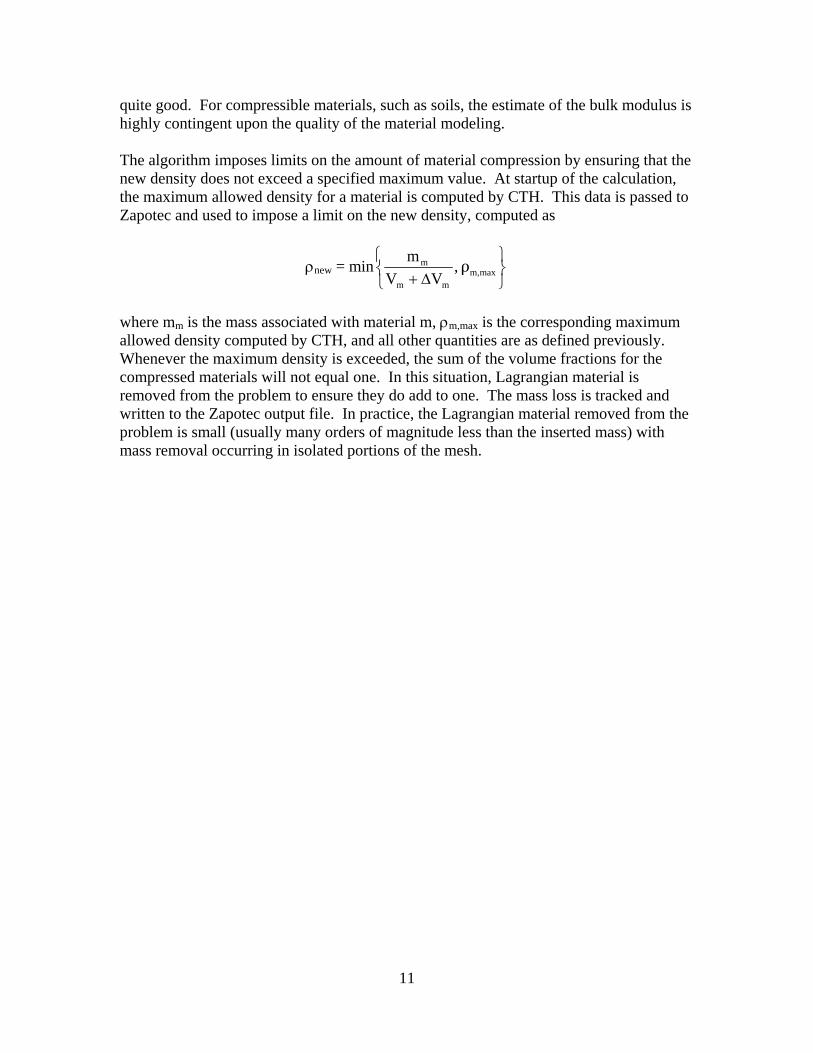
quite good. For compressible materials, such as soils, the estimate of the bulk modulus is highly contingent upon the quality of the material modeling. The algorithm imposes limits on the amount of material compression by ensuring that the new density does not exceed a specified maximum value. At startup of the calculation, the maximum allowed density for a material is computed by CTH. This data is passed to Zapotec and used to impose a limit on the new density, computed as

ρnew = min⎭⎬⎫

⎩⎨⎧

Δ+ maxm,mm

m ρ ,V V

m

where mm is the mass associated with material m, ρm,max is the corresponding maximum allowed density computed by CTH, and all other quantities are as defined previously. Whenever the maximum density is exceeded, the sum of the volume fractions for the compressed materials will not equal one. In this situation, Lagrangian material is removed from the problem to ensure they do add to one. The mass loss is tracked and written to the Zapotec output file. In practice, the Lagrangian material removed from the problem is small (usually many orders of magnitude less than the inserted mass) with mass removal occurring in isolated portions of the mesh.

11

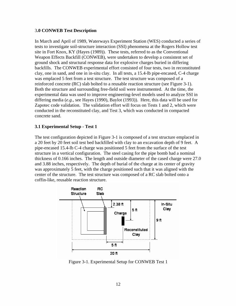
3.0 CONWEB Test Description In March and April of 1989, Waterways Experiment Station (WES) conducted a series of tests to investigate soil-structure interaction (SSI) phenomena at the Rogers Hollow test site in Fort Knox, KY (Hayes (1989)). These tests, referred to as the Conventional Weapon Effects Backfill (CONWEB), were undertaken to develop a consistent set of ground shock and structural response data for explosive charges buried in differing backfills. The CONWEB experimental effort consisted of four tests, two in reconstituted clay, one in sand, and one in in-situ clay. In all tests, a 15.4-lb pipe-encased, C-4 charge was emplaced 5 feet from a test structure. The test structure was composed of a reinforced concrete (RC) slab bolted to a reusable reaction structure (see Figure 3-1). Both the structure and surrounding free-field soil were instrumented. At the time, the experimental data was used to improve engineering-level models used to analyze SSI in differing media (e.g., see Hayes (1990), Baylot (1993)). Here, this data will be used for Zapotec code validation. The validation effort will focus on Tests 1 and 2, which were conducted in the reconstituted clay, and Test 3, which was conducted in compacted concrete sand. 3.1 Experimental Setup - Test 1 The test configuration depicted in Figure 3-1 is composed of a test structure emplaced in a 20 feet by 20 feet soil test bed backfilled with clay to an excavation depth of 9 feet. A pipe-encased 15.4-lb C-4 charge was positioned 5 feet from the surface of the test structure in a vertical configuration. The steel casing for the pipe bomb had a nominal thickness of 0.166 inches. The length and outside diameter of the cased charge were 27.0 and 3.88 inches, respectively. The depth of burial of the charge at its center of gravity was approximately 5 feet, with the charge positioned such that it was aligned with the center of the structure. The test structure was composed of a RC slab bolted onto a coffin-like, reusable reaction structure.

Figure 3-1. Experimental Setup for CONWEB Test 1

12

Only a summary description of the test structure construction is provided here. A detailed description of site preparation and construction can be found in Hayes (1989). The RC slab was 15 feet long, 65 inches high, with a thickness of 4.3 inches. The average unconfined compressive strength of the concrete on the day of the test was 6095 psi. The reinforcement layout for the slab is depicted in Figure 3-2. The reinforcement was composed of Grade 60 No. 3 rebar serving as principal steel along the slab height direction; temperature steel composed of D1 wire (0.113 inch diameter) running along the length direction; and shear steel composed of D3 wire (0.195 inch diameter) running along the slab thickness. The D3 wire was heat treated to conform as closely as possible to Grade 60 steel. The average tensile strength of the principal, temperature, and shear steel was 67,424 psi, 81,667 psi, and 73,222 psi, respectively. The slab had 1.0 percent steel reinforcement, calculated by area along the principal steel direction. The reaction structure was 15 feet long, 65 inches high, and 4 feet deep. The wall thickness was 11 inches. The reaction structure was stated to be heavily reinforced (Hayes (1989)); however, no details were available regarding the reinforcement layout. A 5/8-inch steel plate was attached to the mating surface with the RC slab to ensure a smooth mounting surface as well as provide protection to the reaction structure. Prior to the test, the slab was bolted to the reaction structure with one-inch diameter pre-tensioned bolts. Bolt holes were set at 9-inch intervals along the top and bottom of the reaction structure, resulting in a total of 38 bolts used to connect the slab to the reaction structure. The test structure was emplaced in a 20 by 20 foot test bed excavated to a depth of 9 feet. The test bed was backfilled with reconstituted clay, specified to have four percent or less of air void. The average wet and dry density of the clay was 122.5 lb/ft3 and 99.4 lb/ft3, respectively. The water content was 23.3 percent and the seismic velocity was nominally 1100 ft/sec. Care was taken during backfilling to ensure consistency of the soil properties throughout the test bed. The region outside of the test bed was composed of in-situ clay. Both the structure and surrounding free-field soil was instrumented to obtain ground shock and structure response data. The instrumentation plan is depicted in Figures 3-3 and 3-4. The gage nomenclature is denoted in the figures. Details regarding gage manufacture, mounting, and placement can be found in Hayes (1989).

13

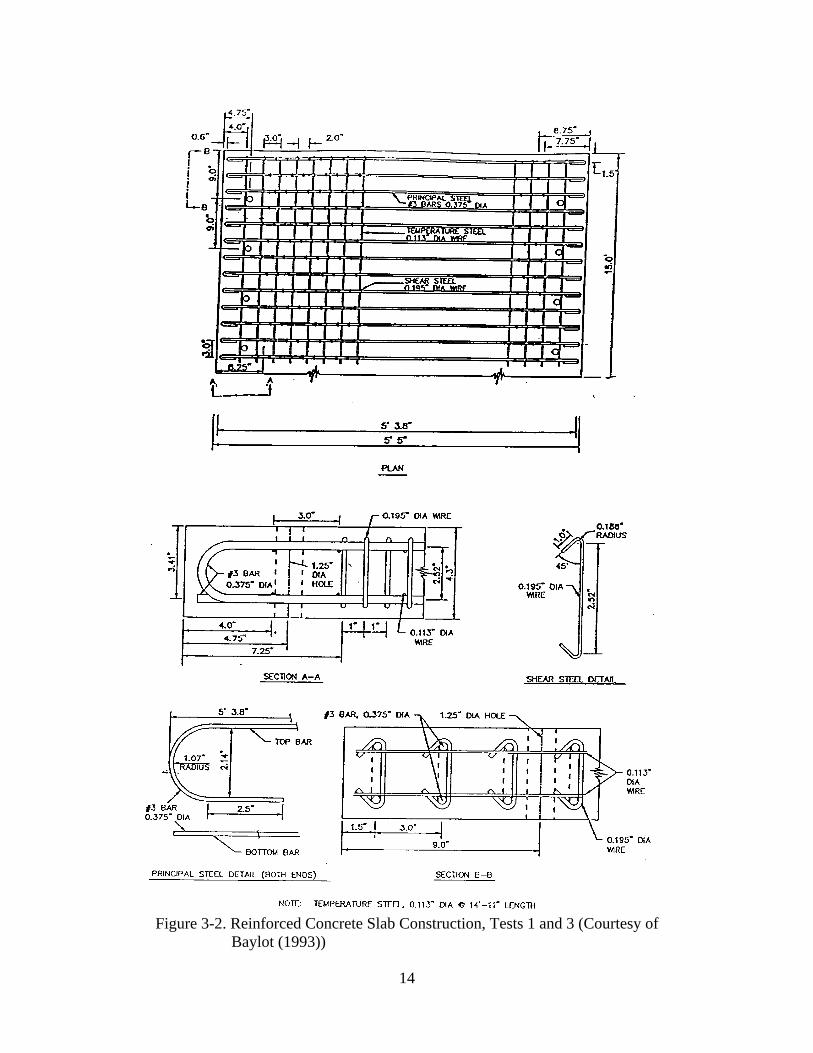
Figure 3-2. Reinforced Concrete Slab Construction, Tests 1 and 3 (Courtesy of

Baylot (1993))

14

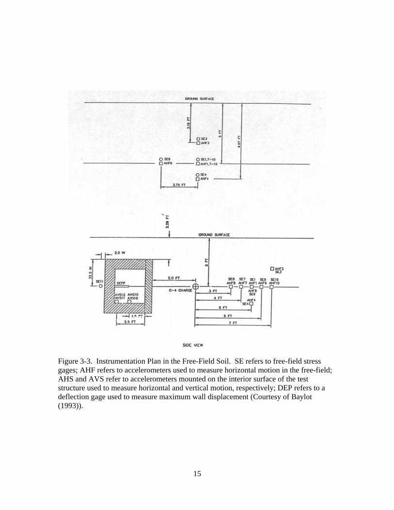
Figure 3-3. Instrumentation Plan in the Free-Field Soil. SE refers to free-field stress gages; AHF refers to accelerometers used to measure horizontal motion in the free-field; AHS and AVS refer to accelerometers mounted on the interior surface of the test structure used to measure horizontal and vertical motion, respectively; DEP refers to a deflection gage used to measure maximum wall displacement (Courtesy of Baylot (1993)).

15

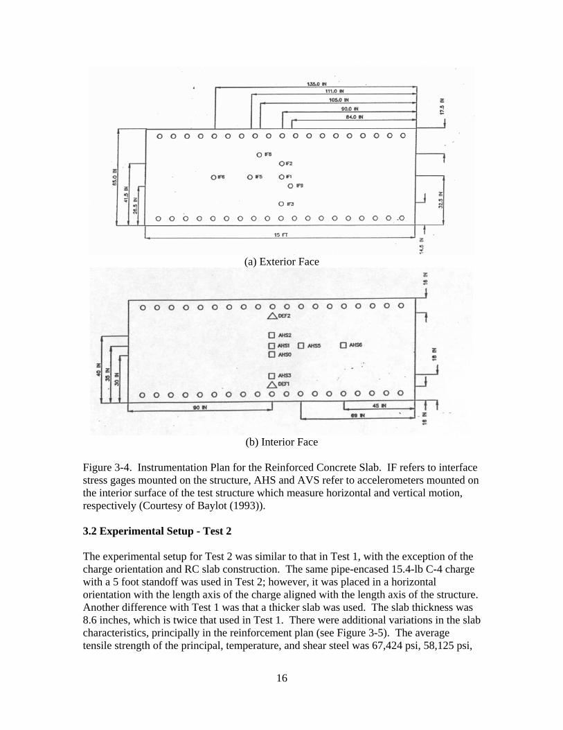
(a) Exterior Face

(b) Interior Face

Figure 3-4. Instrumentation Plan for the Reinforced Concrete Slab. IF refers to interface stress gages mounted on the structure, AHS and AVS refer to accelerometers mounted on the interior surface of the test structure which measure horizontal and vertical motion, respectively (Courtesy of Baylot (1993)). 3.2 Experimental Setup - Test 2 The experimental setup for Test 2 was similar to that in Test 1, with the exception of the charge orientation and RC slab construction. The same pipe-encased 15.4-lb C-4 charge with a 5 foot standoff was used in Test 2; however, it was placed in a horizontal orientation with the length axis of the charge aligned with the length axis of the structure. Another difference with Test 1 was that a thicker slab was used. The slab thickness was 8.6 inches, which is twice that used in Test 1. There were additional variations in the slab characteristics, principally in the reinforcement plan (see Figure 3-5). The average tensile strength of the principal, temperature, and shear steel was 67,424 psi, 58,125 psi,

16

and 58,125 psi, respectively. The slab had 0.5 percent steel reinforcement, calculated by area along the principal steel direction. The average unconfined compressive strength of the concrete on the day of the test was 6398 psi. The structure was emplaced in the excavated test bed in the same manner as described for Test 1. The average wet and dry density of the reconstituted clay in Test 2 was 123.7 lb/ft3 and 100.6 lb/ft3, respectively. The water content was 23.0 percent and the seismic velocity was nominally 1100 ft/sec. The measured soil properties are virtually identical to that in Test 1. The instrumentation plan for the structure was the same as that used in Test 1. However, there were differences in the plan for the free-field instrumentation, which are outlined in Hayes (1989). This will not be discussed here as it is not germane to this analysis. 3.3 Experimental Setup - Test 3 Test 3 used the same experimental setup as Test 1. The major difference between the two was the backfill media, where compacted concrete sand was used for Test 3. The primary goal of this test was to compare backfill effects on the structure response. Both the sand and clay have comparable seismic velocities (on the order of 1100 ft/sec), with the major difference between the two related to their shear response and porosity. The sand has a high-shear strength and porosity, while the shear strength and porosity of the clay is small by comparison. The RC slab design was identical for Tests 1 and 3; however, the concrete strength differed. In Test 3, the average unconfined concrete compressive strength on the day of the test was 5855 psi, which is slightly lower than that in Test 1 (6095 psi). The structure was emplaced in the excavated test bed in the same manner as described for Test 1. The average wet and dry density of the sand in Test 3 was 116.4 lb/ft3 and 110.8 lb/ft3, respectively. The water content was approximately 5.0 percent and the seismic velocity was nominally 1100 ft/sec. The sand is a porous medium having approximately 25.3 percent air void. The instrumentation plan for the structure was the same as that used in Test 1. However, there were differences in the plan for the free-field instrumentation, which are outlined in Hayes (1989). This will not be discussed here as it is not germane to this analysis.

17

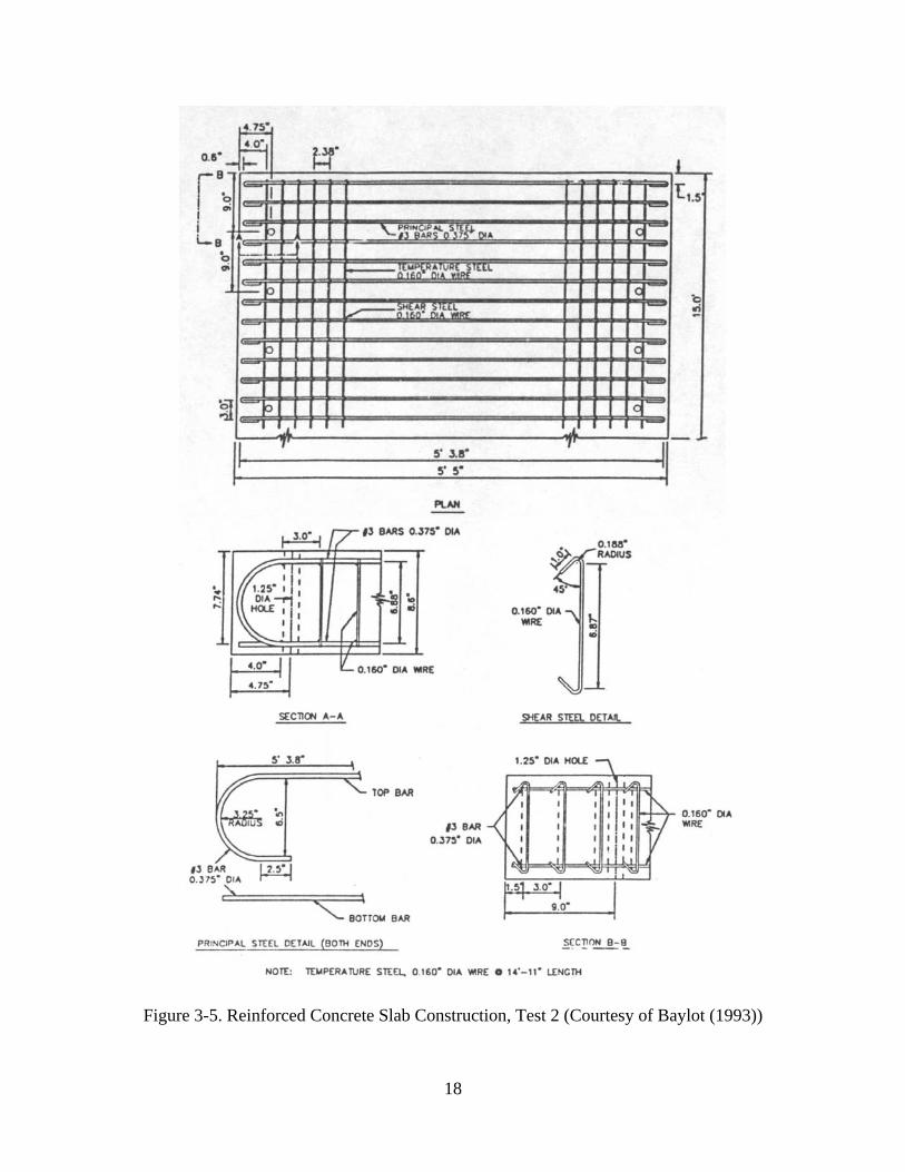
Figure 3-5. Reinforced Concrete Slab Construction, Test 2 (Courtesy of Baylot (1993))

18

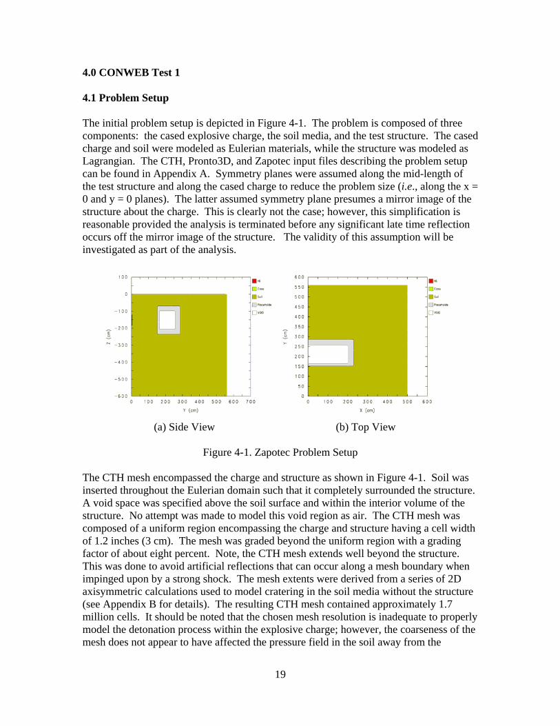
4.0 CONWEB Test 1 4.1 Problem Setup The initial problem setup is depicted in Figure 4-1. The problem is composed of three components: the cased explosive charge, the soil media, and the test structure. The cased charge and soil were modeled as Eulerian materials, while the structure was modeled as Lagrangian. The CTH, Pronto3D, and Zapotec input files describing the problem setup can be found in Appendix A. Symmetry planes were assumed along the mid-length of the test structure and along the cased charge to reduce the problem size (i.e., along the x = 0 and y = 0 planes). The latter assumed symmetry plane presumes a mirror image of the structure about the charge. This is clearly not the case; however, this simplification is reasonable provided the analysis is terminated before any significant late time reflection occurs off the mirror image of the structure. The validity of this assumption will be investigated as part of the analysis.

(a) Side View (b) Top View

Figure 4-1. Zapotec Problem Setup The CTH mesh encompassed the charge and structure as shown in Figure 4-1. Soil was inserted throughout the Eulerian domain such that it completely surrounded the structure. A void space was specified above the soil surface and within the interior volume of the structure. No attempt was made to model this void region as air. The CTH mesh was composed of a uniform region encompassing the charge and structure having a cell width of 1.2 inches (3 cm). The mesh was graded beyond the uniform region with a grading factor of about eight percent. Note, the CTH mesh extends well beyond the structure. This was done to avoid artificial reflections that can occur along a mesh boundary when impinged upon by a strong shock. The mesh extents were derived from a series of 2D axisymmetric calculations used to model cratering in the soil media without the structure (see Appendix B for details). The resulting CTH mesh contained approximately 1.7 million cells. It should be noted that the chosen mesh resolution is inadequate to properly model the detonation process within the explosive charge; however, the coarseness of the mesh does not appear to have affected the pressure field in the soil away from the

19

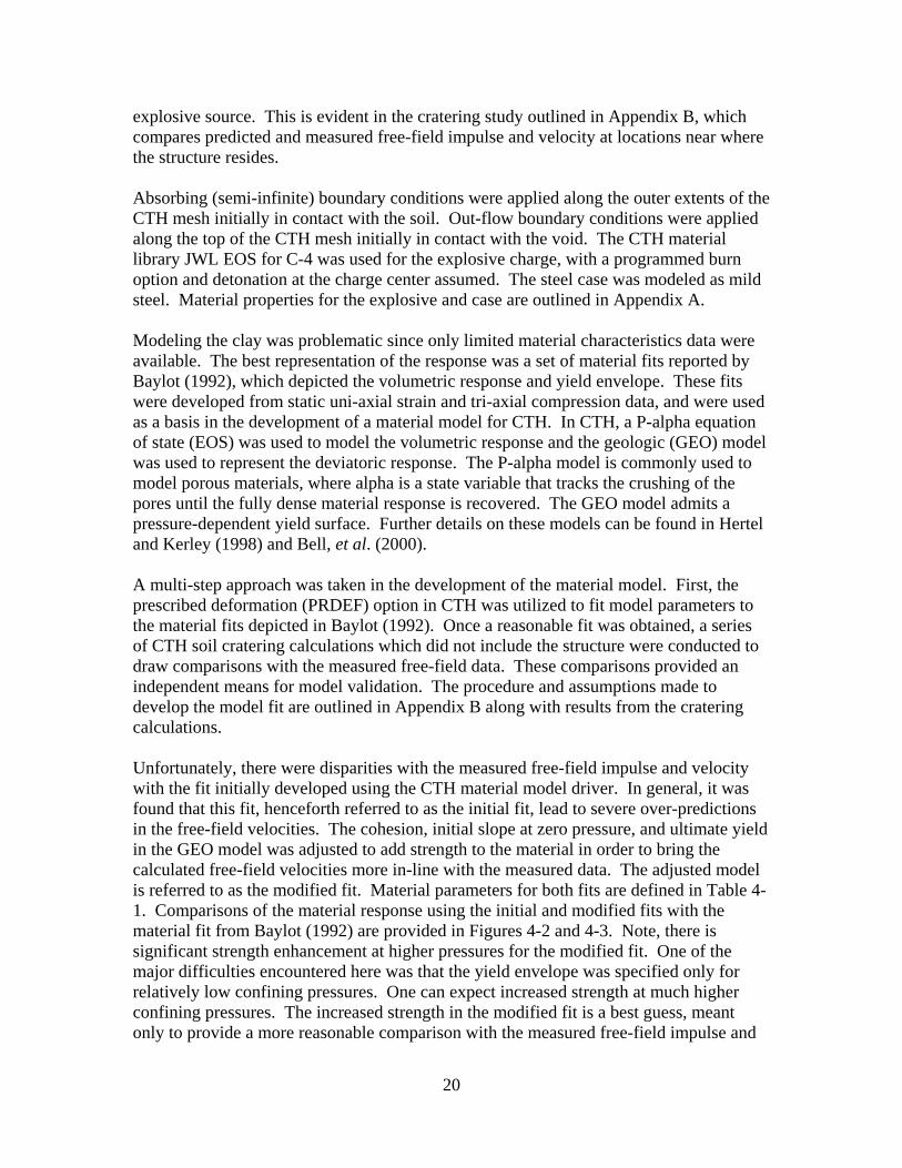
explosive source. This is evident in the cratering study outlined in Appendix B, which compares predicted and measured free-field impulse and velocity at locations near where the structure resides. Absorbing (semi-infinite) boundary conditions were applied along the outer extents of the CTH mesh initially in contact with the soil. Out-flow boundary conditions were applied along the top of the CTH mesh initially in contact with the void. The CTH material library JWL EOS for C-4 was used for the explosive charge, with a programmed burn option and detonation at the charge center assumed. The steel case was modeled as mild steel. Material properties for the explosive and case are outlined in Appendix A. Modeling the clay was problematic since only limited material characteristics data were available. The best representation of the response was a set of material fits reported by Baylot (1992), which depicted the volumetric response and yield envelope. These fits were developed from static uni-axial strain and tri-axial compression data, and were used as a basis in the development of a material model for CTH. In CTH, a P-alpha equation of state (EOS) was used to model the volumetric response and the geologic (GEO) model was used to represent the deviatoric response. The P-alpha model is commonly used to model porous materials, where alpha is a state variable that tracks the crushing of the pores until the fully dense material response is recovered. The GEO model admits a pressure-dependent yield surface. Further details on these models can be found in Hertel and Kerley (1998) and Bell, et al. (2000). A multi-step approach was taken in the development of the material model. First, the prescribed deformation (PRDEF) option in CTH was utilized to fit model parameters to the material fits depicted in Baylot (1992). Once a reasonable fit was obtained, a series of CTH soil cratering calculations which did not include the structure were conducted to draw comparisons with the measured free-field data. These comparisons provided an independent means for model validation. The procedure and assumptions made to develop the model fit are outlined in Appendix B along with results from the cratering calculations. Unfortunately, there were disparities with the measured free-field impulse and velocity with the fit initially developed using the CTH material model driver. In general, it was found that this fit, henceforth referred to as the initial fit, lead to severe over-predictions in the free-field velocities. The cohesion, initial slope at zero pressure, and ultimate yield in the GEO model was adjusted to add strength to the material in order to bring the calculated free-field velocities more in-line with the measured data. The adjusted model is referred to as the modified fit. Material parameters for both fits are defined in Table 4-1. Comparisons of the material response using the initial and modified fits with the material fit from Baylot (1992) are provided in Figures 4-2 and 4-3. Note, there is significant strength enhancement at higher pressures for the modified fit. One of the major difficulties encountered here was that the yield envelope was specified only for relatively low confining pressures. One can expect increased strength at much higher confining pressures. The increased strength in the modified fit is a best guess, meant only to provide a more reasonable comparison with the measured free-field impulse and

20

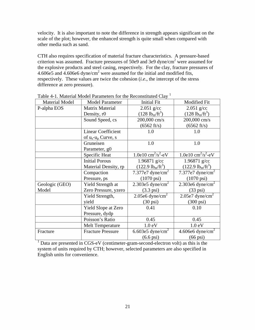
velocity. It is also important to note the difference in strength appears significant on the scale of the plot; however, the enhanced strength is quite small when compared with other media such as sand. CTH also requires specification of material fracture characteristics. A pressure-based criterion was assumed. Fracture pressures of 50e9 and 3e9 dyne/cm2 were assumed for the explosive products and steel casing, respectively. For the clay, fracture pressures of 4.606e5 and 4.606e6 dyne/cm2 were assumed for the initial and modified fits, respectively. These values are twice the cohesion (i.e., the intercept of the stress difference at zero pressure). Table 4-1. Material Model Parameters for the Reconstituted Clay 1

Material Model Model Parameter Initial Fit Modified Fit P-alpha EOS Matrix Material

Density, r0 2.051 g/cc

(128 lbm/ft3) 2.051 g/cc

(128 lbm/ft3) Sound Speed, cs 200,000 cm/s

(6562 ft/s) 200,000 cm/s

(6562 ft/s) Linear Coefficient

of us-up Curve, s 1.0 1.0

Gruneisen Parameter, g0

1.0 1.0

Specific Heat 1.0e10 cm2/s2-eV 1.0e10 cm2/s2-eV Initial Porous

Material Density, rp 1.96871 g/cc

(122.9 lbm/ft3) 1.96871 g/cc

(122.9 lbm/ft3) Compaction

Pressure, ps 7.377e7 dyne/cm2

(1070 psi) 7.377e7 dyne/cm2

(1070 psi) Geologic (GEO) Model

Yield Strength at Zero Pressure, yzero

2.303e5 dyne/cm2

(3.3 psi) 2.303e6 dyne/cm2

(33 psi) Yield Strength,

yield 2.05e6 dyne/cm2

(30 psi) 2.05e7 dyne/cm2

(300 psi) Yield Slope at Zero

Pressure, dydp 0.41 0.10

Poisson’s Ratio 0.45 0.45 Melt Temperature 1.0 eV 1.0 eV Fracture Fracture Pressure 6.603e5 dyne/cm2

(6.6 psi) 4.606e6 dyne/cm2

(66 psi) 1 Data are presented in CGS-eV (centimeter-gram-second-electron volt) as this is the system of units required by CTH; however, selected parameters are also specified in English units for convenience.

21

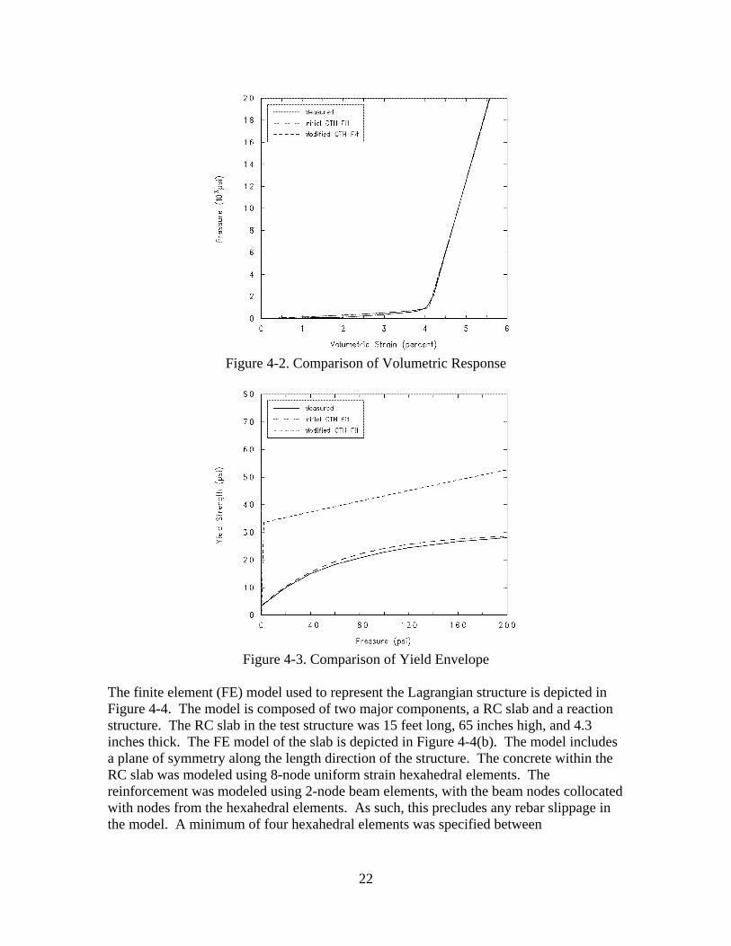
Figure 4-2. Comparison of Volumetric Response

Figure 4-3. Comparison of Yield Envelope

The finite element (FE) model used to represent the Lagrangian structure is depicted in Figure 4-4. The model is composed of two major components, a RC slab and a reaction structure. The RC slab in the test structure was 15 feet long, 65 inches high, and 4.3 inches thick. The FE model of the slab is depicted in Figure 4-4(b). The model includes a plane of symmetry along the length direction of the structure. The concrete within the RC slab was modeled using 8-node uniform strain hexahedral elements. The reinforcement was modeled using 2-node beam elements, with the beam nodes collocated with nodes from the hexahedral elements. As such, this precludes any rebar slippage in the model. A minimum of four hexahedral elements was specified between

22

reinforcement layers, admitting a nominal element size of 0.75 inches (1.9 cm). There were approximately 80,000 elements in the mesh. The reinforcement plan was not exactly followed in the model development. In the test slab, the shear steel had an alternating layout for each layer (see Figure 3-2). In the model, the shear steel spacing within a layer was assumed constant throughout the slab. This simplification was necessary since Pronto3D requires that beam and hexahedral element nodes be collocated. The true layout of the shear steel could not be modeled with the chosen mesh resolution within the concrete. Also, the hooked ends of for the reinforcement could not be modeled for similar reasons. The reaction structure was modeled using hexahedral elements with a fairly coarse mesh (see Figure 4-4(a)). No reinforcement plan was available for the reaction structure. Consequently, reinforcement was not included in the model of the reaction structure. To compensate for the loss of added structural integrity, the concrete strength was substantially increased to enhance its stiffness. This is a reasonable assumption since the reaction structure is designed to be reusable and only serves as a back-stop for the RC slab. Baylot (1993) made a similar assumption in previous analyses, which proved to be reasonable for this application. The reaction structure has a steel facing plate at the interface with the RC slab. This plate was included in the FE model and was discretized using 4-node uniform strain shell elements, based on a Key-Hoff formulation. The bolts used to attach the RC slab to the reaction structure were modeled using 2-node beam elements. The concrete response was modeled using the Karagozian and Case (K&C) constitutive model (Malvar, et al. (1997) and Attaway, et al. (2000)). This model can be described as a concrete plasticity model, which decouples the volumetric and deviatoric response. A tabulated equation of state defines the pressure as a function of the current and previous minimum volumetric strains. The deviatoric portion of the model admits three yield surfaces: the yield failure surface, the maximum failure surface, and the residual failure surface. These failure surfaces serve to track the damage evolution within the concrete. The concrete model is complex and interested readers are directed to Malvar, et al. (1997) and Attaway, et al. (2000) for further details. There are many versions of the K&C concrete model. The version implemented into Pronto3D allows the user to input a few selected material parameters (unconfined compressive strength, density, Poisson ratio, fractional dilatancy, and maximum aggregate size) which are used by the model to automatically develop additional material data used internally by the code (e.g., determination of a strain rate enhancement factor, which is derived from the unconfined compressive strength and elastic modulus). The internal data is tuned to a “WSMR” concrete, which was characterized as part of a series of blast-on-structure tests conducted at the White Sands Missile Range (WSMR), NM. Caution should be exercised when using an automated model since no two concretes are exactly alike. For this analysis, there was little choice since only the unconfined compressive strength was available for the concrete used in the CONWEB tests. User

23

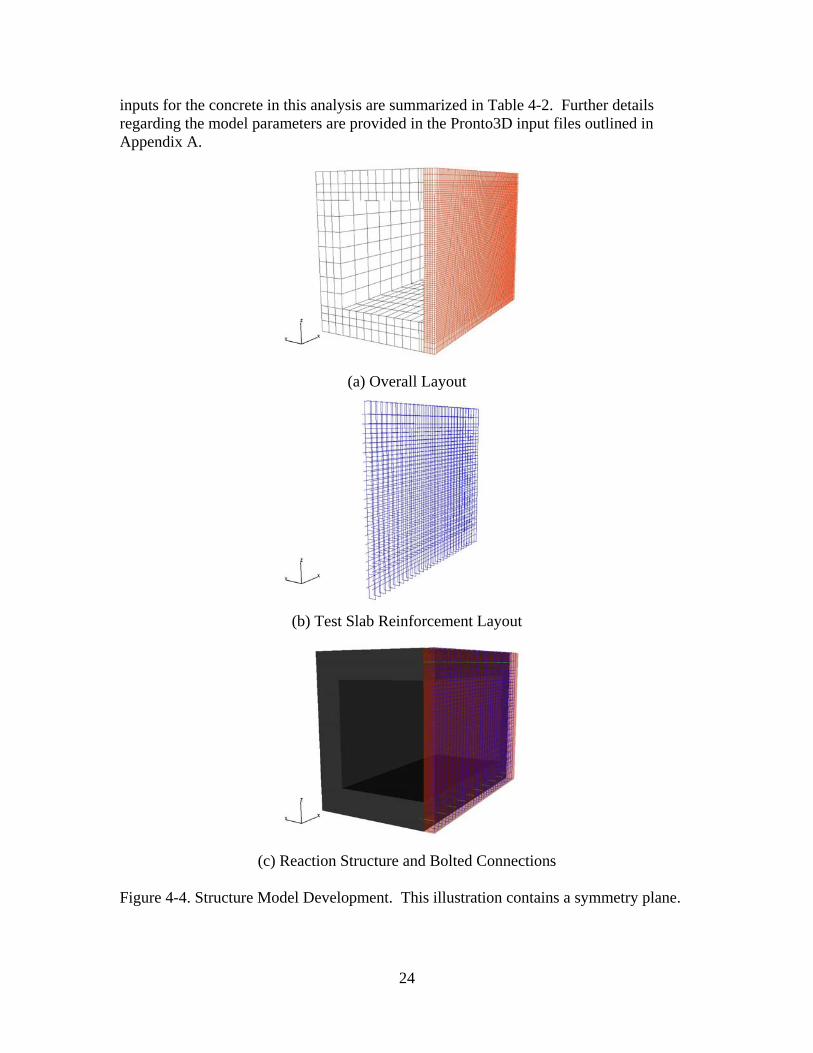
inputs for the concrete in this analysis are summarized in Table 4-2. Further details regarding the model parameters are provided in the Pronto3D input files outlined in Appendix A.

(a) Overall Layout

(b) Test Slab Reinforcement Layout

(c) Reaction Structure and Bolted Connections

Figure 4-4. Structure Model Development. This illustration contains a symmetry plane.

24

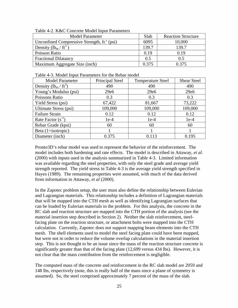
Table 4-2. K&C Concrete Model Input Parameters Model Parameter Slab Reaction Structure

Unconfined Compressive Strength, fc’ (psi) 6095 10,000 Density (lbm / ft3 ) 139.7 139.7 Poisson Ratio 0.19 0.19 Fractional Dilatancy 0.5 0.5 Maximum Aggregate Size (inch) 0.375 0.375 Table 4-3. Model Input Parameters for the Rebar model

Model Parameter Principal Steel Temperature Steel Shear Steel Density (lbm / ft3) 490 490 490 Young’s Modulus (psi) 29e6 29e6 29e6 Poissons Ratio 0.3 0.3 0.3 Yield Stress (psi) 67,422 81,667 73,222 Ultimate Stress (psi) 109,000 109,000 109,000 Failure Strain 0.12 0.12 0.12 Rate Factor (s-1) 1e-4 1e-4 1e-4 Rebar Grade (kpsi) 60 60 60 Beta (1=isotropic) 1 1 1 Diameter (inch) 0.375 0.113 0.195 Pronto3D’s rebar model was used to represent the behavior of the reinforcement. The model includes both hardening and rate effects. The model is described in Attaway, et al. (2000) with inputs used in the analysis summarized in Table 4-3. Limited information was available regarding the steel properties, with only the steel grade and average yield strength reported. The yield stress in Table 4-3 is the average yield strength specified in Hayes (1989). The remaining properties were assumed, with much of the data derived from information in Attaway, et al (2000). In the Zapotec problem setup, the user must also define the relationship between Eulerian and Lagrangian materials. This relationship includes a definition of Lagrangian materials that will be mapped into the CTH mesh as well as identifying Lagrangian surfaces that can be loaded by Eulerian materials in the problem. For this analysis, the concrete in the RC slab and reaction structure are mapped into the CTH portion of the analysis (see the material insertion step described in Section 2). Neither the slab reinforcement, steel-facing plate on the reaction structure, or attachment bolts were mapped into the CTH calculation. Currently, Zapotec does not support mapping beam elements into the CTH mesh. The shell elements used to model the steel facing plate could have been mapped, but were not in order to reduce the volume overlap calculations in the material insertion step. This is not thought to be an issue since the mass of the reaction structure concrete is significantly greater than that of the facing plate (12,699 versus 434 lbs). However, it is not clear that the mass contribution from the reinforcement is negligible. The computed mass of the concrete and reinforcement in the RC slab model are 2059 and 148 lbs, respectively (note, this is really half of the mass since a plane of symmetry is assumed). So, the steel comprised approximately 7 percent of the mass of the slab.

25

Although the mass contribution is not substantial, it is not negligible. Furthermore, there is expected to be substantially more reinforcement in the reaction structure. Unfortunately, the amount cannot be quantified since the reinforcement details were not available. The implications of not mapping the reinforcement into the CTH calculation are unclear. Intuitively, one would expect a less-massive structure to exhibit greater deformation. This has implications in the CTH portion of the Zapotec calculation where a greater predicted slab motion would affect the neighboring interface pressures computed by CTH. In turn, this would affect the loading on the Lagrangian structure. These concerns will be investigated in the analysis. The exterior surfaces of the RC slab and reaction structure were specified as Eulerian contact surfaces. Euler contact surfaces (akin to the definition of slidelines for Lagrangian contact) are used to define surfaces that can be loaded by neighboring Eulerian material. Zapotec allows several options for force application. Of interest here is the weighting scheme used for determining the stress state in the neighboring Eulerian material. Bessette, et al. (2003) examined the influence of weighting scheme for an air blast application. The analysis suggested that it is best to derive the Eulerian stress state from the cell forward of the Lagrangian structure (i.e., from a CTH cell which is comprised of only Eulerian material). This approach is taken for this analysis by selecting force option 2 in the Zapotec input. By default, the Zapotec analysis invokes Lagrangian subcycling as described in Section 2. The duration of the analysis was 20 msec, which coincides with the duration of recorded data in the test. 4.2 Analysis Results A considerable amount of data was gathered during the test. These data include pressure and velocity histories in the free-field, interface pressure data at the surface of the RC slab, and structural response data from accelerometers embedded in both the slab and reaction structure. In addition, post-test measurements were made of the soil crater and structure damage. Comparisons with the free-field data are discussed in Appendix B. These comparisons are based on standalone CTH calculations that did not include the structure in the setup. No attempt was made to model the free-field region in the Zapotec analysis. For the Zapotec analysis, data comparisons will fall into two categories, comparisons of the interface pressures computed by CTH and the structural response computed by Pronto3D. These comparisons will be discussed separately. Only limited digitized test data were available from WES. When the data records were not available, they were obtained by digitizing figures from the test report (Hayes (1989)). To simplify the process, only smooth data such as impulse or velocity were digitized. This was sufficient for the purposes of this analysis. Before proceeding with the data analysis, it is first useful to summarize the outcome of the test.

26

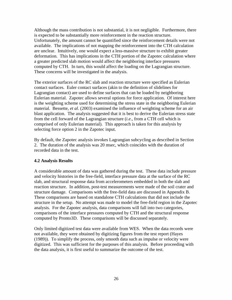
4.2.1 Summary of Test Results The explosive event resulted in the formation of a crater having an apparent depth of approximately 7.87 feet. The apparent crater width and length were 13 and 13 feet, respectively. The width direction is defined along a direction parallel to the long axis of the structure, while the crater length is defined along a direction perpendicular to the structure. Severe damage of the RC slab was noted, with an 18 by 51 inch breach observed in the front face of the slab (see Figures 4-5 and 4-6). In addition, reinforcement bars were broken along the top and bottom supports near the center of the slab. The measured deflection from the outside face to the deformed rebar at the slab center was approximately 19 inches. Significant cracking was noted along the entire length of the slab on both the front and rear faces. Comparisons with pre-test elevation measurements indicated the top of the reaction structure moved downwards an average of 1.89 inches and rotated slightly towards the charge (i.e., the structure rotated in a counter-clockwise direction with respect to the view in Figure 4-1(a)).

Figure 4-5. Front Face Damage to RC Slab (Courtesy of Hayes (1990))

Figure 4-6. Interior View of RC Slab (Courtesy of Hayes (1990))

27

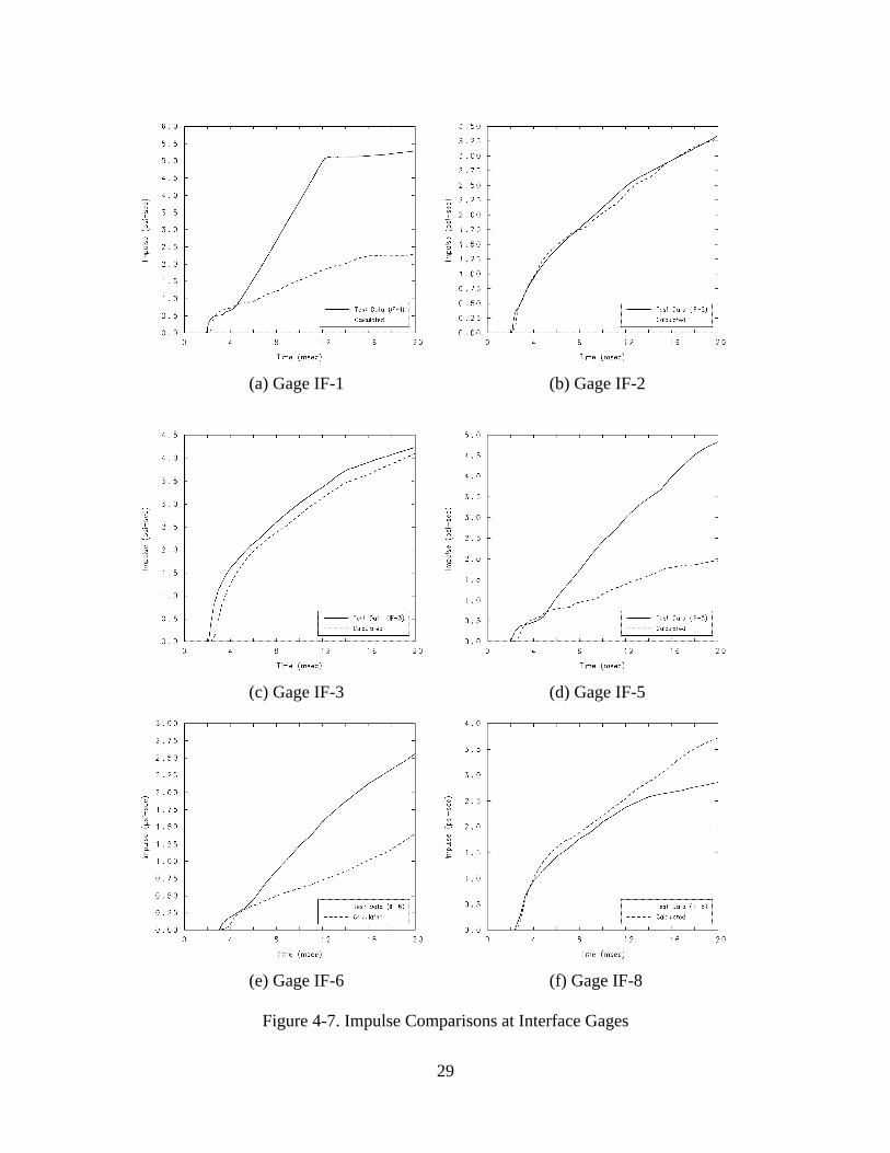
4.2.2 Interface Impulse Comparisons Comparisons of the measured and calculated impulse at the interface gage locations are provided Figure 4-7. The calculated results are derived from tracers embedded in the CTH mesh. These tracers were offset 5 cm from the structure to ensure they did not reside initially in a mixed material cell. Also, the noi or no interpolation option was set in the CTH control input. CTH pressures were integrated to obtain the specific impulse. As discussed earlier, the calculations utilized the modified fit for the reconstituted clay. One generally notes a slight lag in the calculated time-of-arrival, which can be attributed to a lack of adequate mesh resolution. One also notes obvious disparities with the impulse at several gage locations. In particular, significant differences are noted with gages IF-1, IF-5, and IF-6. The differences are best explained by viewing the pressure data. For example, consider the pressure history measured at gage IF-1 (see Figure 4-8). The pressure history is characterized by an initial peak followed by a plateau region after 4 msec. Baylot (1993) suggests the plateau region is an artifact of the instrumentation, likely introduced by the gage being squeezed as the slab deformed. A similar, but much less distinct, behavior was noted in the pressure records for gages IF-5 and IF-6. Given the similarity in gage response, it is likely the same explanation can apply for gages IF-5 and IF-6. For gage IF-8, there was no hint of gage squeezing in the pressure record and no reason can be given for the disparity in the impulse. If one considers the impulse record only to the point where gage squeezing occurs, then one might conclude there is reasonably good correlation of the measured and calculated impulses, with a slight tendency to over-predict the impulse (e.g., consider a time-shifted impulse history for IF-1 up until the point where gage squeezing becomes evident). This is a subjective statement; however, it seems reasonable and consistent for the cases where gage squeezing occurs.

28

(a) Gage IF-1 (b) Gage IF-2

(c) Gage IF-3 (d) Gage IF-5

(e) Gage IF-6 (f) Gage IF-8

Figure 4-7. Impulse Comparisons at Interface Gages

29

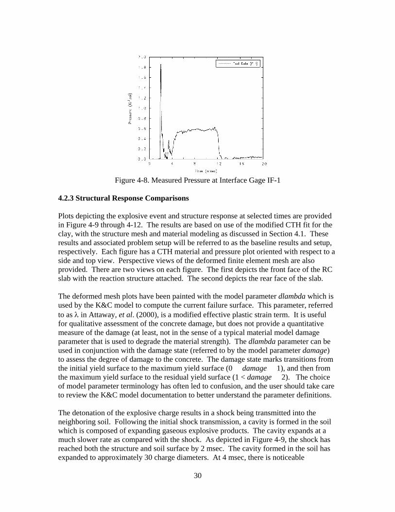
Figure 4-8. Measured Pressure at Interface Gage IF-1

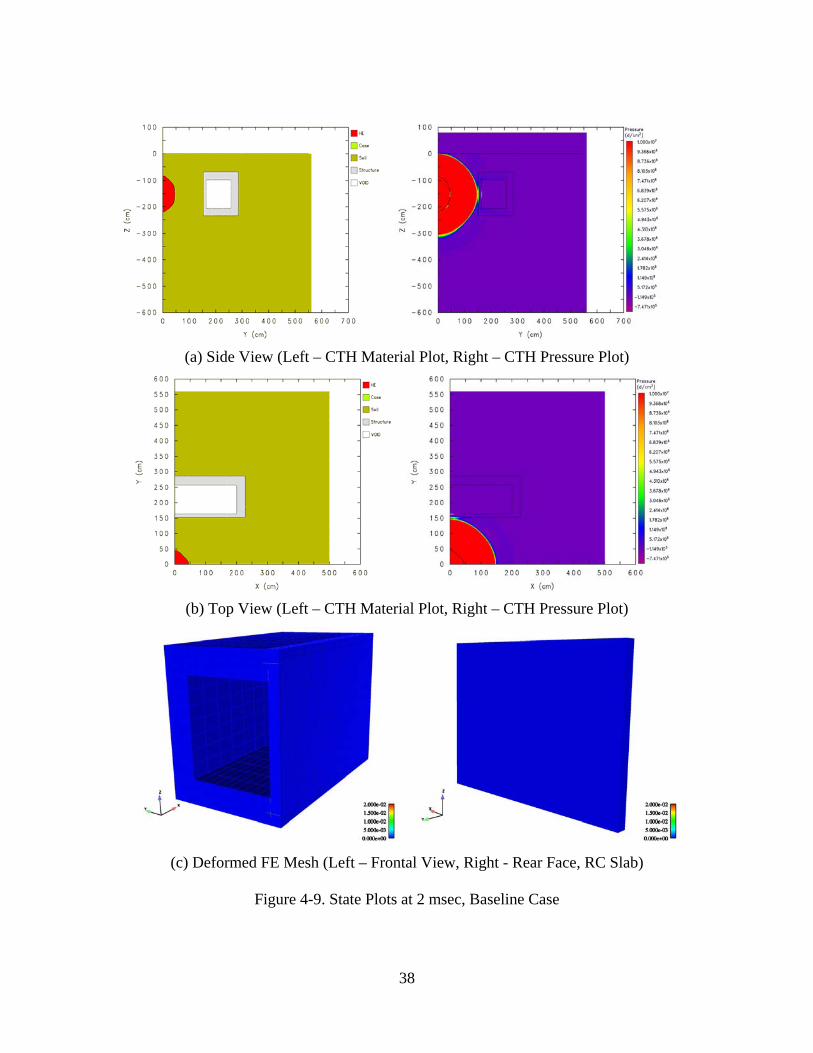
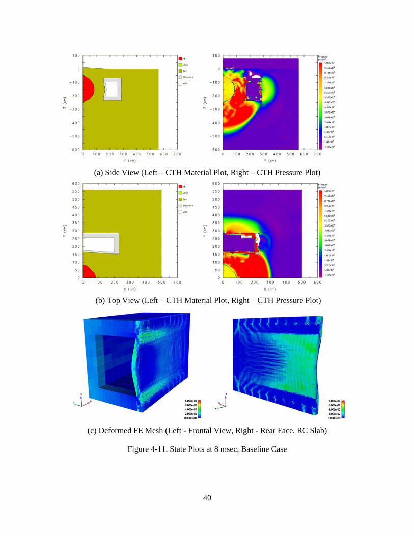
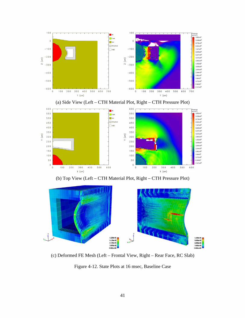
4.2.3 Structural Response Comparisons Plots depicting the explosive event and structure response at selected times are provided in Figure 4-9 through 4-12. The results are based on use of the modified CTH fit for the clay, with the structure mesh and material modeling as discussed in Section 4.1. These results and associated problem setup will be referred to as the baseline results and setup, respectively. Each figure has a CTH material and pressure plot oriented with respect to a side and top view. Perspective views of the deformed finite element mesh are also provided. There are two views on each figure. The first depicts the front face of the RC slab with the reaction structure attached. The second depicts the rear face of the slab. The deformed mesh plots have been painted with the model parameter dlambda which is used by the K&C model to compute the current failure surface. This parameter, referred to as λ in Attaway, et al. (2000), is a modified effective plastic strain term. It is useful for qualitative assessment of the concrete damage, but does not provide a quantitative measure of the damage (at least, not in the sense of a typical material model damage parameter that is used to degrade the material strength). The dlambda parameter can be used in conjunction with the damage state (referred to by the model parameter damage) to assess the degree of damage to the concrete. The damage state marks transitions from the initial yield surface to the maximum yield surface (0 � damage � 1), and then from the maximum yield surface to the residual yield surface (1 < damage � 2). The choice of model parameter terminology has often led to confusion, and the user should take care to review the K&C model documentation to better understand the parameter definitions. The detonation of the explosive charge results in a shock being transmitted into the neighboring soil. Following the initial shock transmission, a cavity is formed in the soil which is composed of expanding gaseous explosive products. The cavity expands at a much slower rate as compared with the shock. As depicted in Figure 4-9, the shock has reached both the structure and soil surface by 2 msec. The cavity formed in the soil has expanded to approximately 30 charge diameters. At 4 msec, there is noticeable

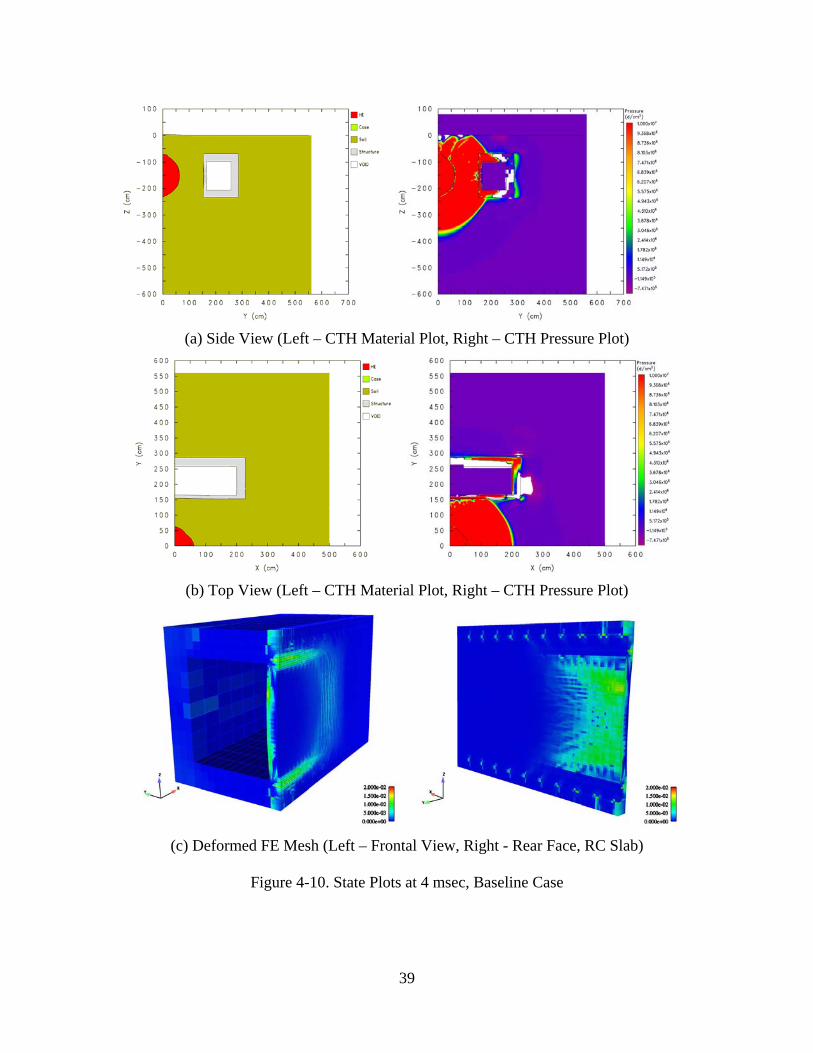
30

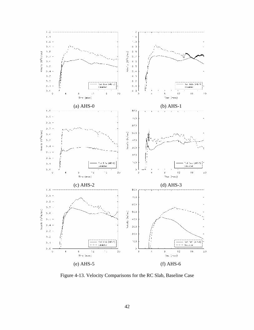
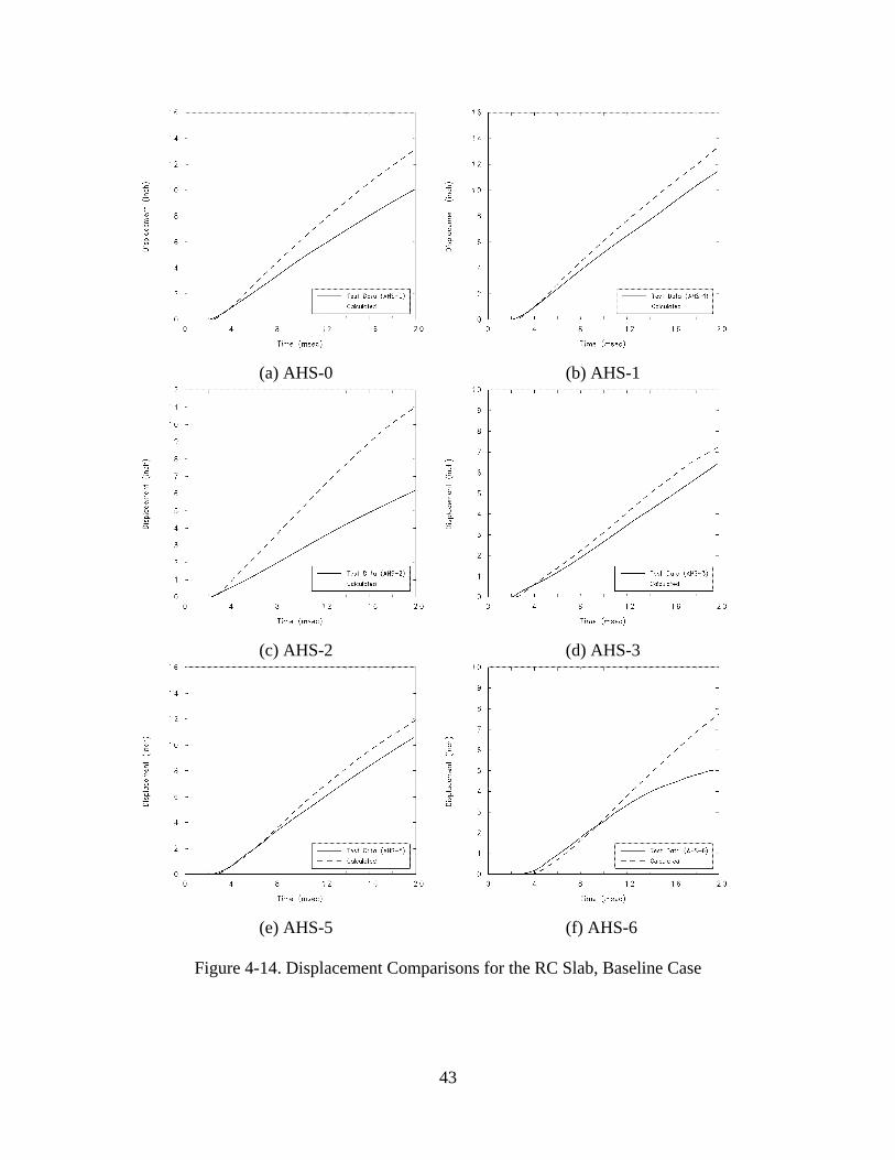
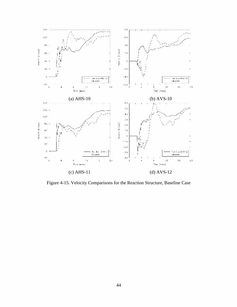
deformation of the structure (see Figure 4-10). There is also bulging at the soil surface. The continued loading on the structure as depicted in Figures 4-11 and 4-12 results in increased structure deformation. In the figures, one notes loading on the front face of the slab as well as the rear surface of the reaction structure. The latter is a consequence of soil resistance to the structure’s rigid body motion. There is also increased bulging at the soil surface. Over time, the soil overburden will be ejected upwards to form a crater. The calculation was not carried out long enough to capture the cratering phenomena. The calculation was only run for 20 msec, the extent of the available test data. Review of the data up to this point suggests the slab will be breached. The size of the breach hole cannot be determined from the analysis; however, it is evident there will be extensive damage along the slab center as well as at the end supports near the structure centerline (see the deformed mesh plots). There is also evidence of separation between the concrete slab and facing plate on the reaction structure. This is due to localized rotation of the slab along the supported edge as well as deformation of the bolted connections. Structural response comparisons are made at selected accelerometer locations in both the slab and reaction structure. In the slab, accelerometer locations AHS-0, AHS-1, AHS-2, AHS-3, AHS-5, and AHS-6 are of interest. In the reaction structure, accelerometer locations AHS-10, AHS-11, AVS-10, and AVS-12 are of interest. Nodal history data from the FE mesh was stored for comparison with the experimental data. Comparisons are made for both the velocity and displacement histories. In the evaluation of the test data, there is limited confidence in the measured late-time velocity (and displacement) data (Baylot (2004)). Unfortunately, there were no data available to independently check integrated accelerometer data (e.g., deflection gages along no-breached portions of the slab). Also, since the structure was breached, it is unknown as to when the accelerometers became detached from the structure. Hence, there is greater confidence in the initial peak velocities derived from the accelerometer records. Comparisons of structure velocities and displacements in the slab are provided in Figures 4-13 and 4-14. The rise time in the velocity compares well between the calculation and measured data; however, the initial peak velocity is generally over-predicted. In turn, the velocity over-prediction leads to an over-prediction in the calculated displacements. Additional comparisons for the reaction structure are provided in Figures 4-15 and 4-16. There is reasonably good correlation with the measured data, suggesting Zapotec is providing a good estimate of the loading on the rear surface of the reaction structure. Given the good correlation of data for the reaction structure, one can focus attention on error associated with modeling the loading on the RC slab and/or its response as the likely culprit for the disparities in the structure velocity. The reason for the disparities in the slab response is unclear. Comparisons for the interface impulse suggest reasonably good correlation of the results, with a tendency to slightly over-predict the impulse (assuming one omits that portion of the record affected by gage squeezing). It is not clear that the slight over-prediction in impulse alone can explain the disparity in the structure velocities. It is likely that additional modeling

31

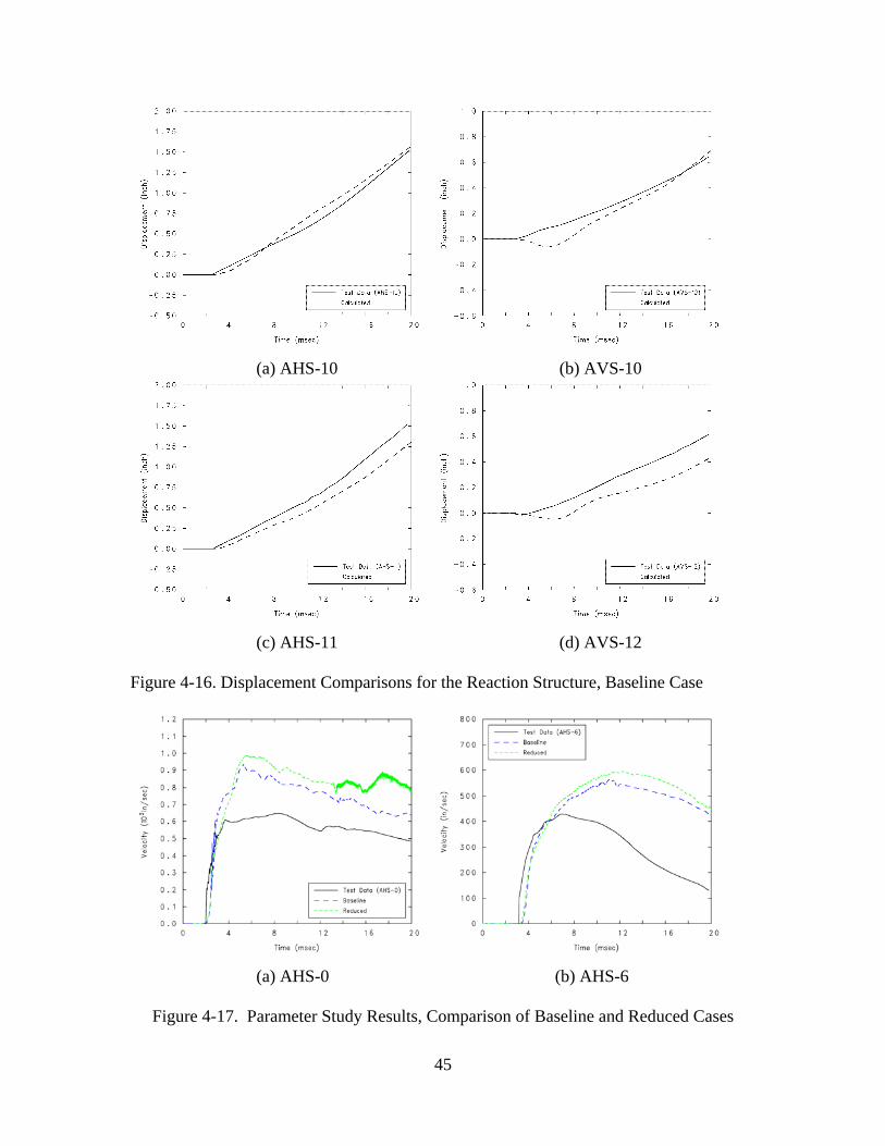
uncertainty has been introduced into the analysis. This modeling uncertainty will be investigated by a parametric study, which will primarily focus on variations in model inputs for the structure. Additional parameter variations associated with the CTH model development and Zapotec inputs will also be considered. The latter variations were considered to gain insight into the coupling algorithm and potential interplay between computational domains when modeling this class of problem. The problem setup for the parameter study is similar to that used for the baseline, with the exception that a coarser CTH mesh was considered. The revised CTH mesh has a 2 inch (5 cm) resolution in the interaction region between the blast and structure. This setup will be referred to as the reduced problem. The reduced CTH mesh contained approximately 628,000 cells. A summary of the parameter study variations is provided in Table 4-4. Each parameter variation is given a name, signifying the input data affected (e.g., case Pronto-1 denotes a parameter variation in the Pronto3D input). To simplify matters, comparisons are made for the velocity and displacement data at accelerometer locations AHS-0 and AHS-6. These locations were chosen because they exhibit bounds on the maximum and minimum slab response. The results of the parameter study are summarized in Figures 4-17 through 4-21 and Table 4-5. The calculated displacements in Table 4-5 are generally close to one another, with the final value usually within 5 inches of that measured. One should bear in mind that displacement is a doubly-integrated quantity, and that different velocity histories can reach the same end displacement. One should also recall there is greater confidence in the initial peak velocity as opposed to the later-time velocity history (Baylot (2004)). Hence, more emphasis will be placed on comparisons of the peak structure velocity. The influence of CTH mesh resolution is best illustrated in Figure 4-17 where velocity comparisons are shown for the baseline and reduced cases. One notes that a slightly higher velocity is attained with the coarser mesh calculation. The finer mesh associated with the baseline problem is better able to model the distribution of loading over the structure. This is an important point since the loading will be redistributed as the structure deforms. Although no attempt was made to assess convergence, it is conjectured that a finer CTH mesh would provide better correlation of the velocities; however, it is not believed the improvement would be enough to explain the disparity with the test data. Another likely source of modeling error resides with the development of the FE model. There are many issues here, including modeling the constitutive response of both the concrete and reinforcement, mesh resolution, and modeling the bolted connection between the RC slab and reaction structure. The Pronto-1 case addresses modeling error associated with the reinforcement (see Figure 4-18). Here, the reinforcement was modeled as a purely elastic-plastic material with the yield strength enhanced by 20 percent to account for rate effects. One notes little difference in results compared with the reduced case for the first 12 msec of the event; however, differences are noted

32

thereafter, with a stiffer structure response noted at AHS-0 and a less stiff response noted at AHS-6 as compared with the reduced case. Cases Pronto-2 through Pronto-6 focus on issues associated with modeling the concrete response (see Figures 4-18 and 4-19). As with the Pronto-1 case, there is little difference in results for the first 10 to 12 msec of the event. Thereafter, there is a noticeable departure in results from the reduced case. For this problem, neither rate effects (Pronto-4 Case) nor variations in concrete strength (Pronto Cases 5 and 6) appear to significantly affect the outcome. The initial fractional dilatancy term (omega) has more of an effect. Attaway, et al. (2000) define this term as the fraction associativity term, which is the initial ratio of the plastic volume strain increment to that which would occur if the plastic flow were fully associated in the hydrostatic plane. The initial value is used until the stress point reaches the maximum failure surface, after which the current value of omega decays to zero in order to reduce dilatancy. From the velocity comparisons in Figure 4-18, it appears that in regions where there is significant damage to the structure, i.e., near AHS-0, increasing omega results in a less stiff response of the structure (at least at later times). In regions exhibiting less damage, i.e., near AHS-6, the opposite appears to be the case, where increasing omega seems to result in enhanced stiffness. The K&C concrete model is quite complex and the details regarding the omega term and its implementation are not well understood by this author. There is clearly room for future work in better understanding the constitutive model. The Pronto-7 case considers a variation in the prescribed initial concrete density. For this case, the density was increased from 139.6 lb/ft3 to 145 lb/ft3. In hindsight, the latter value seemed a more reasonable estimate of concrete density. The increased density leads to a 3.8 percent increase in the mass of the slab. In the discussion of the Zapotec problem setup, there were concerns about not mapping the reinforcement mass, which was approximately 7 percent of the mass of the slab. It was conjectured that a less-massive structure inserted into the CTH mesh during the material insertion step might exhibit greater deformation. In turn, this could affect the neighboring interface pressure distribution computed by CTH. The Pronto-7 case indirectly addresses this concern, where the slight increase in mapped slab mass exhibits a negligible influence on the slab response. The Pronto-8 case was run to specifically address error associated with modeling the bolted connections between the slab and reaction structure. In the FE model, the bolts were modeled using beam elements whose nodes were collocated in both the slab and reaction structure. In the reduced problem, the slab was allowed to detach and rotate about the facing plate on the reaction structure, with resistance provided by the beam elements representing the bolts. The use of a fixed contact precludes any separation between the slab and facing plate. Thus any localized rotation is due to rotation within the reaction structure. As expected, the fixed contact leads to less displacement of the slab at the two accelerometer locations; however, the differences are small, suggesting that the FE model provided a reasonably good representation of the stiff bolted connections associated with the test structure.

33

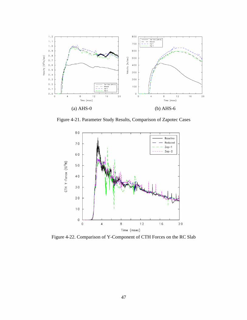
The Pronto-9 case addresses mesh resolution issues associated with the slab. In this case, the slab was better resolved, allowing a minimum of six elements between reinforcement bars. As with other cases, one sees differing trends based on the two locations. At AHS-0, a higher velocity is attained with the finer mesh. In contrast, at AHS-6, the opposite is observed. Regardless, the differences are not large at either accelerometer location, suggesting the baseline FE model provides reasonable results. Additional cases investigating modeling error in the CTH portion of the analysis are illustrated in Figure 4-20. The CTH-1 case investigates the validity of assuming a plane of symmetry opposite the face of the structure, i.e., along a plane at y = 0 in Figure 4-1. This was accomplished by extending the CTH mesh along the negative y-direction to include the free-field region. Modeling the free-field region appears to have little effect on the calculation, at least for the time duration of interest here. The second case, CTH-2, has a much more noticeable effect where the results are based on using the initial material fit for the reconstituted clay. As discussed in Appendix B, the use of this fit led to significant over-predictions in both the free-field impulse and velocity. It is not surprising that its use leads to higher computed structure velocities, since the loading is over-estimated. Cases Zap-1 and Zap-2 investigate one of the user input options available for controlling a Zapotec calculation (see Figure 4-21). Here, the focus is on selecting the number of allowed Lagrangian subcycles. Recall, the time step taken by Zapotec is generally controlled by CTH, since the stable time step for Pronto3D is usually smaller than that for CTH. This is indeed the case here following initial startup of the calculation. The net effect of reducing the number of allowed Lagrangian subcycles is to scale back the time step taken by CTH, while increasing the amount of subcycling allows CTH to operate at its maximum possible stable time step. The calculated structure velocity is affected to some degree by limiting the subcycling. In Figure 4-21, there is a noticeable difference in results at AHS-6 for the Zap-1 case, where a higher velocity is attained as compared with the reduced problem. Similar behavior is noted at AHS-0, but to a lesser degree. It is often instructive to look at the forces applied on the Lagrangian structure, which are referred to as the CTH forces. This can provide insight into non-physical loadings on the structure arising from localized “hot” zones in the CTH mesh. These hot zones are regions of artificially high pressure which can be generated by poor energy or density states in an Eulerian cell. The user can check for these localized hot zones by reviewing the spatial plot data (i.e., the CTH pressure and Pronto3D nodal force plots). The problem with using the spatial plot data is that these results are taken at a snapshot in time. The localized hot zones are transient and it is usually a matter of luck with seeing them in the spatial plot data. Pronto3D allows the user to save the CTH force history data. These forces are a global summation of forces applied to either a material surface or a pre-defined sideset as a function of time. In general, localized hot zones will result in applied forces that are much higher than that observed elsewhere in the force-time history. Thus, review of the CTH force data provides a useful tool to assess the validity of a Zapotec calculation.

34

The y-component of the CTH forces applied on the RC slab surface is shown in Figure 4-22 for several cases of interest. The results do not indicate any localized hot zones (it is usually obvious); however, the force profiles are noisy. It has been conjectured that the noisy behavior is largely due to the over-filled cell treatment (see discussion in Section 2). An over-filled cell arises when the volume of the resident Eulerian material and the inserted Lagrangian material exceeds the fixed, Eulerian cell volume. The algorithm for treating over-filled cells compresses materials so that the sum of their new volumes equals the total cell volume. A weighting scheme based on the material volume divided by its bulk modulus is used to determine the compression of individual materials in the cell. When a material is compressed, its pressure is increased in proportion to its bulk modulus and change in volume (Δp = K (ΔV/V)). The internal energy is also increased in proportion to the volumetric compression, i.e., the PΔV work. The increased pressure state in the Eulerian materials affects the stress state in the region, which in turn, affects the computed forces on the neighboring Lagrangian structure. The over-filled cell treatment is a non-smooth process in which the degree of material compression can fluctuate from time step to time step. This contributes to the noisy profile for the applied forces. The influence of various input options on the CTH forces is examined in Figure 4-22. The behavior for the baseline and reduced cases is very similar, with the exception that higher loads are noted with the baseline case very early in the calculation. The reduced and Zap-2 cases exhibit a comparable behavior; however, a somewhat erratic behavior is noted with the Zap-1 case where the calculation is limited to 5 subcycles. The maximum allowed CTH time step attained following the initial startup of the calculation is on the order of 7.5 μsec. This value was derived from the Zap-2 case, which essentially allows unlimited subcycling. Also, this value is only 55 percent of the Courant limit (by default, CTH applies a time step scale factor of 0.55 for 3D calculations). In comparison, representative CTH time steps for the reduced and Zap-1 cases were 5.1 and 2.8 μsec, respectively. Intuitively, one might expect that a lower CTH (and hence Zapotec) time step would lead to less compression in over-filled cells and a smoother force profile in time. However, the calculation suggests that a drastic cut back in the allowed CTH stable time step can have a negative effect on the smoothness of the loading. There appears to be no clear cut answer for the noisiness in the calculated forces as they appear to be influenced by both the over-filled cell treatment as well as stability concerns in the Eulerian domain. This is a common predicament faced by developers linking codes based on vastly different numerical solution approaches. Further review of the data indicates the cost of the calculation is significantly increased as the CTH time step is decreased (see Table 4-6). It is clear that better performance (in both accuracy and reduced CPU) is obtained if CTH can operate at or near its maximum possible time step. However, it is not clear how to set up the problem to take advantage of this observation a priori since estimates of initial times steps are usually not indicative of what is actually used later in the calculation. There remains much work left to do in this area.

35

In addition to benchmarking, it was also of interest to assess the computational costs as this is a key issue for production computing. Timing data summarizing CPU costs, number of computational cycles, and problem size are provided in Table 4-6 for selected cases. All analyses were run on the SNL QT cluster, which is composed of a 16-node AlphaServer™ ES45 system. Each node has four processors with an Alpha 21264 C68/1000-MHz CPU having 8-MB L2 Dual Rate Cache and 32-GB memory, running under Tru 64 Unix V5.1A. The analyses were conducted in parallel using 16 processors. The CPU time for the reduced problem was on the order of 9 hours. This time is typical for most of the parameter variations considered. As expected, CPU times increased when a finer mesh was used and decreased as the amount of Lagrangian subcycling increased. The grind time, defined here as the CPU time per processor divided by the number of Zapotec cycles times the number of CTH cells, can be used as a measure of performance. Comparable grind times are noted, with the exception of the Pronto-9 case. The volume overlap calculation is computationally expensive, representing a significant portion of the cost of a Zapotec calculation. This is reflected in the increased grind time as there are more Lagrangian finite elements considered in the overlap calculation.

36

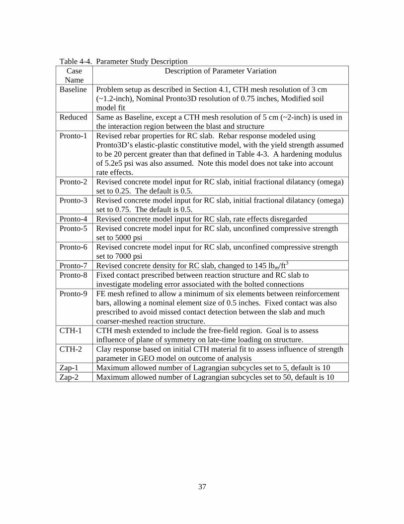
Table 4-4. Parameter Study Description

Case Name

Description of Parameter Variation

Baseline Problem setup as described in Section 4.1, CTH mesh resolution of 3 cm (~1.2-inch), Nominal Pronto3D resolution of 0.75 inches, Modified soil model fit

Reduced Same as Baseline, except a CTH mesh resolution of 5 cm (~2-inch) is used in the interaction region between the blast and structure

Pronto-1 Revised rebar properties for RC slab. Rebar response modeled using Pronto3D’s elastic-plastic constitutive model, with the yield strength assumed to be 20 percent greater than that defined in Table 4-3. A hardening modulus of 5.2e5 psi was also assumed. Note this model does not take into account rate effects.

Pronto-2 Revised concrete model input for RC slab, initial fractional dilatancy (omega) set to 0.25. The default is 0.5.

Pronto-3 Revised concrete model input for RC slab, initial fractional dilatancy (omega) set to 0.75. The default is 0.5.

Pronto-4 Revised concrete model input for RC slab, rate effects disregarded Pronto-5 Revised concrete model input for RC slab, unconfined compressive strength

set to 5000 psi Pronto-6 Revised concrete model input for RC slab, unconfined compressive strength

set to 7000 psi Pronto-7 Revised concrete density for RC slab, changed to 145 lbm/ft3 Pronto-8 Fixed contact prescribed between reaction structure and RC slab to

investigate modeling error associated with the bolted connections Pronto-9 FE mesh refined to allow a minimum of six elements between reinforcement

bars, allowing a nominal element size of 0.5 inches. Fixed contact was also prescribed to avoid missed contact detection between the slab and much coarser-meshed reaction structure.

CTH-1 CTH mesh extended to include the free-field region. Goal is to assess influence of plane of symmetry on late-time loading on structure.

CTH-2 Clay response based on initial CTH material fit to assess influence of strength parameter in GEO model on outcome of analysis

Zap-1 Maximum allowed number of Lagrangian subcycles set to 5, default is 10 Zap-2 Maximum allowed number of Lagrangian subcycles set to 50, default is 10

37

(a) Side View (Left – CTH Material Plot, Right – CTH Pressure Plot)

(b) Top View (Left – CTH Material Plot, Right – CTH Pressure Plot)

(c) Deformed FE Mesh (Left – Frontal View, Right - Rear Face, RC Slab)

Figure 4-9. State Plots at 2 msec, Baseline Case

38

(a) Side View (Left – CTH Material Plot, Right – CTH Pressure Plot)

(b) Top View (Left – CTH Material Plot, Right – CTH Pressure Plot)

(c) Deformed FE Mesh (Left – Frontal View, Right - Rear Face, RC Slab)

Figure 4-10. State Plots at 4 msec, Baseline Case

39

(a) Side View (Left – CTH Material Plot, Right – CTH Pressure Plot)

(b) Top View (Left – CTH Material Plot, Right – CTH Pressure Plot)

(c) Deformed FE Mesh (Left - Frontal View, Right - Rear Face, RC Slab)

Figure 4-11. State Plots at 8 msec, Baseline Case

40

(a) Side View (Left – CTH Material Plot, Right – CTH Pressure Plot)

(b) Top View (Left – CTH Material Plot, Right – CTH Pressure Plot)

(c) Deformed FE Mesh (Left – Frontal View, Right – Rear Face, RC Slab)

Figure 4-12. State Plots at 16 msec, Baseline Case

41

(a) AHS-0 (b) AHS-1

(c) AHS-2 (d) AHS-3

(e) AHS-5 (f) AHS-6

Figure 4-13. Velocity Comparisons for the RC Slab, Baseline Case

42

(a) AHS-0 (b) AHS-1

(c) AHS-2 (d) AHS-3

(e) AHS-5 (f) AHS-6

Figure 4-14. Displacement Comparisons for the RC Slab, Baseline Case

43

(a) AHS-10 (b) AVS-10

(c) AHS-11 (d) AVS-12

Figure 4-15. Velocity Comparisons for the Reaction Structure, Baseline Case

44

(a) AHS-10 (b) AVS-10

(c) AHS-11 (d) AVS-12 Figure 4-16. Displacement Comparisons for the Reaction Structure, Baseline Case

(a) AHS-0 (b) AHS-6

Figure 4-17. Parameter Study Results, Comparison of Baseline and Reduced Cases

45

(a) AHS-0 (b) AHS-6

Figure 4-18. Parameter Study Results, Comparison of Pronto Cases 1 to 4

(a) AHS-0 (b) AHS-6

Figure 4-19. Parameter Study Results, Comparison of Pronto Cases 5 to 9

(a) AHS-0 (b) AHS-6

Figure 4-20. Parameter Study Results, Comparison of CTH Cases

46

(a) AHS-0 (b) AHS-6

Figure 4-21. Parameter Study Results, Comparison of Zapotec Cases

Figure 4-22. Comparison of Y-Component of CTH Forces on the RC Slab

47

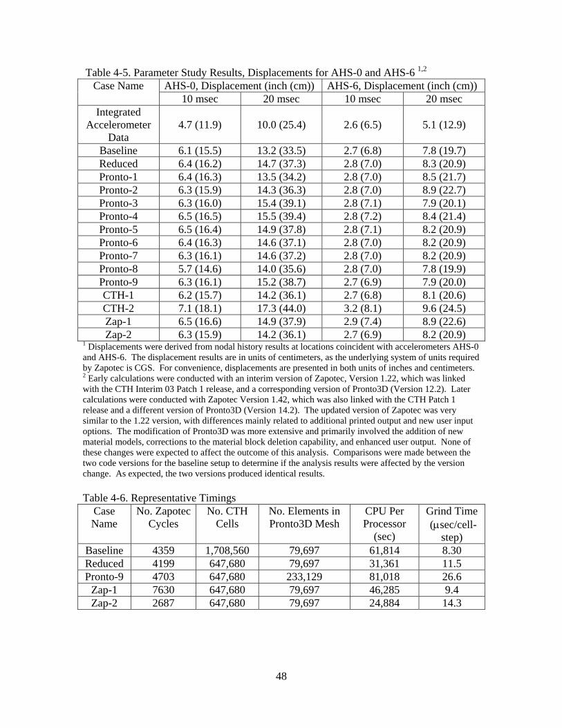
Table 4-5. Parameter Study Results, Displacements for AHS-0 and AHS-6 1,2

AHS-0, Displacement (inch (cm)) AHS-6, Displacement (inch (cm)) Case Name 10 msec 20 msec 10 msec 20 msec

Integrated Accelerometer

Data

4.7 (11.9)

10.0 (25.4)

2.6 (6.5)

5.1 (12.9)

Baseline 6.1 (15.5) 13.2 (33.5) 2.7 (6.8) 7.8 (19.7) Reduced 6.4 (16.2) 14.7 (37.3) 2.8 (7.0) 8.3 (20.9) Pronto-1 6.4 (16.3) 13.5 (34.2) 2.8 (7.0) 8.5 (21.7) Pronto-2 6.3 (15.9) 14.3 (36.3) 2.8 (7.0) 8.9 (22.7) Pronto-3 6.3 (16.0) 15.4 (39.1) 2.8 (7.1) 7.9 (20.1) Pronto-4 6.5 (16.5) 15.5 (39.4) 2.8 (7.2) 8.4 (21.4) Pronto-5 6.5 (16.4) 14.9 (37.8) 2.8 (7.1) 8.2 (20.9) Pronto-6 6.4 (16.3) 14.6 (37.1) 2.8 (7.0) 8.2 (20.9) Pronto-7 6.3 (16.1) 14.6 (37.2) 2.8 (7.0) 8.2 (20.9) Pronto-8 5.7 (14.6) 14.0 (35.6) 2.8 (7.0) 7.8 (19.9) Pronto-9 6.3 (16.1) 15.2 (38.7) 2.7 (6.9) 7.9 (20.0) CTH-1 6.2 (15.7) 14.2 (36.1) 2.7 (6.8) 8.1 (20.6) CTH-2 7.1 (18.1) 17.3 (44.0) 3.2 (8.1) 9.6 (24.5) Zap-1 6.5 (16.6) 14.9 (37.9) 2.9 (7.4) 8.9 (22.6) Zap-2 6.3 (15.9) 14.2 (36.1) 2.7 (6.9) 8.2 (20.9)

1 Displacements were derived from nodal history results at locations coincident with accelerometers AHS-0 and AHS-6. The displacement results are in units of centimeters, as the underlying system of units required by Zapotec is CGS. For convenience, displacements are presented in both units of inches and centimeters. 2 Early calculations were conducted with an interim version of Zapotec, Version 1.22, which was linked with the CTH Interim 03 Patch 1 release, and a corresponding version of Pronto3D (Version 12.2). Later calculations were conducted with Zapotec Version 1.42, which was also linked with the CTH Patch 1 release and a different version of Pronto3D (Version 14.2). The updated version of Zapotec was very similar to the 1.22 version, with differences mainly related to additional printed output and new user input options. The modification of Pronto3D was more extensive and primarily involved the addition of new material models, corrections to the material block deletion capability, and enhanced user output. None of these changes were expected to affect the outcome of this analysis. Comparisons were made between the two code versions for the baseline setup to determine if the analysis results were affected by the version change. As expected, the two versions produced identical results. Table 4-6. Representative Timings

Case Name

No. Zapotec Cycles

No. CTH Cells

No. Elements in Pronto3D Mesh

CPU Per Processor

(sec)

Grind Time (μsec/cell-

step) Baseline 4359 1,708,560 79,697 61,814 8.30 Reduced 4199 647,680 79,697 31,361 11.5 Pronto-9 4703 647,680 233,129 81,018 26.6

Zap-1 7630 647,680 79,697 46,285 9.4 Zap-2 2687 647,680 79,697 24,884 14.3

48

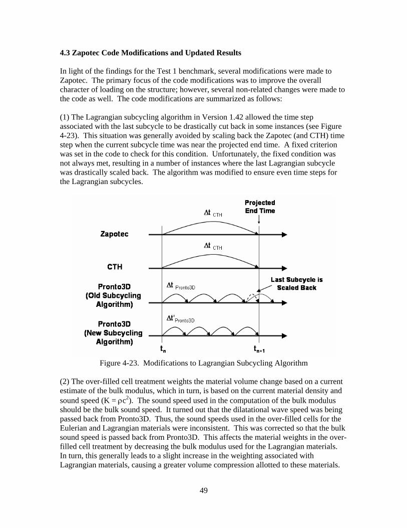
4.3 Zapotec Code Modifications and Updated Results In light of the findings for the Test 1 benchmark, several modifications were made to Zapotec. The primary focus of the code modifications was to improve the overall character of loading on the structure; however, several non-related changes were made to the code as well. The code modifications are summarized as follows: (1) The Lagrangian subcycling algorithm in Version 1.42 allowed the time step associated with the last subcycle to be drastically cut back in some instances (see Figure 4-23). This situation was generally avoided by scaling back the Zapotec (and CTH) time step when the current subcycle time was near the projected end time. A fixed criterion was set in the code to check for this condition. Unfortunately, the fixed condition was not always met, resulting in a number of instances where the last Lagrangian subcycle was drastically scaled back. The algorithm was modified to ensure even time steps for the Lagrangian subcycles.

Figure 4-23. Modifications to Lagrangian Subcycling Algorithm

(2) The over-filled cell treatment weights the material volume change based on a current estimate of the bulk modulus, which in turn, is based on the current material density and sound speed (K = ρc2). The sound speed used in the computation of the bulk modulus should be the bulk sound speed. It turned out that the dilatational wave speed was being passed back from Pronto3D. Thus, the sound speeds used in the over-filled cells for the Eulerian and Lagrangian materials were inconsistent. This was corrected so that the bulk sound speed is passed back from Pronto3D. This affects the material weights in the over-filled cell treatment by decreasing the bulk modulus used for the Lagrangian materials. In turn, this generally leads to a slight increase in the weighting associated with Lagrangian materials, causing a greater volume compression allotted to these materials.

49

(3) Enhanced diagnostic output was added to gain further insights into the over-filled cell treatment. Concurrent benchmarks involving penetration of an essentially rigid penetrator into low-strength grout have suggested there can be excessive over-compression of Eulerian materials as a result of the over-filled cell treatment (Hollenshead, et al. (2004)). The degree of material compression is limited by a maximum allowed density, which is supplied by CTH at startup of the calculation. This value has been observed to be physically unrealistic for most applications involving penetration, and likely blast loading as well. A new option was added to the Zapotec keyword input, allowing the user to control the maximum allowed material density used in the over-filled cell treatment. The Zapotec keyword for this option is “rho_max <Euler material ID> <maximum density>”. In the over-filled cell algorithm, the new density resulting from the material compression is never allowed to exceed the specified value. The Test 1 benchmark was rerun with the updated version of Zapotec, which has been named Version 1.6. This version was also linked with the Interim 03 Patch 1 release of CTH. Typical structural response results for the updated code are provided in Figure 4-24. These results compare the baseline problem setup run with both Zapotec Version 1.42 and 1.6. One notes very little difference in results at the two gage locations. This was typical of results at the other gage locations in both the slab and reaction structure. Comparisons for the computed forces on the slab are provided in Figure 4-25. One notes the Version 1.6 calculation exhibits a higher peak initial force. The reason is not altogether clear, but is related to the bug fix for getting the bulk sound speed from Pronto3D. This was confirmed by incremental testing of the code changes. One also notes less noise in the force history. This is likely due to the changes in the Lagrangian subcycling algorithm. A set of excursion calculations was also run to investigate limiting the material density for soil in the over-filled cell treatment. Three calculations were conducted setting the maximum density to 2.25, 2.5, and 3.0 g/cm3. The default value supplied by CTH was 1969 g/cm3, which is unrealistic. The updated diagnostic output provides a count on the occurrences in which the specified maximum density is exceeded. The maximum density was exceeded 30,490, 12,420, and 0 times for the specified values of 2.25, 2.5, and 3.0 g/cm3, respectively. These numbers are relatively small when put in the context of occurrences per computational cycle, which indicates a maximum average count of 7.3 times per cycle for the specified maximum density of 2.25 g/cm3. In general, the warning messages were written for cells residing along the upper edge of the structure. There did not appear to be any problem with cells near the free-span area of the slab. The velocity and displacement data at the slab and reaction structure gage locations was also reviewed. The results were independent of the choice of maximum density, suggesting the problem noted with excess compression in the penetration studies was not an issue here. However, the treatment of mixed Euler/Lagrange cells is still a research issue and is under investigation.

50

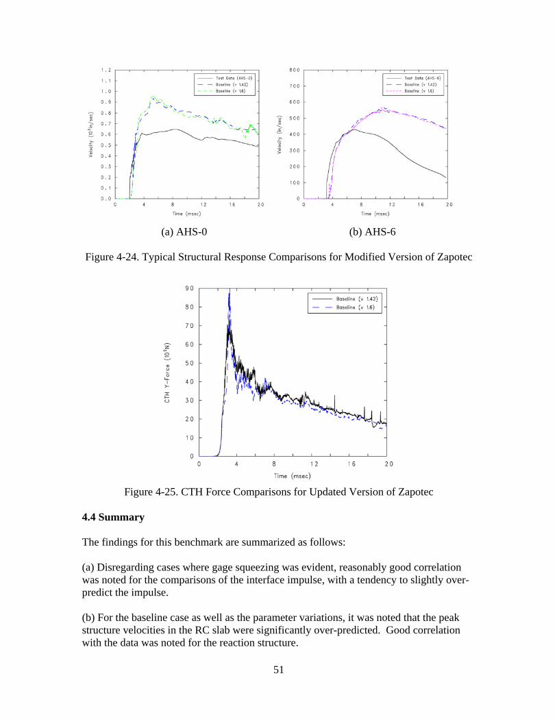
(a) AHS-0 (b) AHS-6 Figure 4-24. Typical Structural Response Comparisons for Modified Version of Zapotec

Figure 4-25. CTH Force Comparisons for Updated Version of Zapotec

4.4 Summary The findings for this benchmark are summarized as follows: (a) Disregarding cases where gage squeezing was evident, reasonably good correlation was noted for the comparisons of the interface impulse, with a tendency to slightly over-predict the impulse. (b) For the baseline case as well as the parameter variations, it was noted that the peak structure velocities in the RC slab were significantly over-predicted. Good correlation with the data was noted for the reaction structure.

51

(c) A portion of the parameter study focused on errors associated with modeling the RC slab. Specifically, variations in concrete model inputs, mesh resolution, and contact definition were of interest. Differences in the structure velocity histories were noted; however, these differences were small in comparison to the disparity with the measured data. One can conclude that modeling error associated with the slab is not a major issue for this benchmark. This is an important point as one could expect more of an influence of the various input options for problems where there is less of an over-match of the loading on the structure. (d) Better comparisons were noted with the finer CTH mesh (3 versus 5 cm resolution for the baseline and reduced cases, respectively). This is not surprising since the finer mesh can better capture the redistribution of stresses in the soil as the structure deforms. In turn, this leads to a more accurate assessment of loading on the structure. However, the reduced case did provide reasonable results and was suitable for the parameter study. (e) The influence of Lagrangian subcycling on the calculation was also investigated. The best performance (both in accuracy and reduced CPU) was obtained when CTH was allowed to operate at or near its maximum possible time step. The implications are that unlimited subcycling should be allowed. However, one must temper this notion by recalling that the loading determined at the first Lagrangian subcycle is applied to all remaining subcycles. Inaccuracies can arise if the loading varies substantially in time. In this situation, the user can minimize the amount of subcycling by better resolving the CTH mesh. (f) The parameter study suggested the material modeling for the soil had the greatest influence on the predicted peak velocities for the slab. The soil model parameters were developed based on limited data and are only expected to approximate the soil response. (g) Both Zapotec and Pronto3D were updated based on the initial findings. Improvements were made to the Lagrangian subcycling algorithm to ensure the time step associated with the last subcycle was not artificially cut off. There was also a bug fix in the sound speed retrieved from Pronto3D for the inserted Lagrangian materials. The bulk sound speed is now returned from Pronto3D, which is consistent with what is obtained from CTH. The code modifications appeared to reduce the noise in the computed forces on the slab, but had little effect on the calculated structure response.

52

5.0 CONWEB Test 2 5.1 Problem Setup The problem setup for Test 2 is comparable to that for Test 1, with some differences. The differences between the two are: (1) the same pipe-encased 15.4-lb C-4 charge was used, but set in a horizontal orientation with the length axis of the charge aligned with the length axis of the test structure, (2) the RC slab in Test 2 was thicker (8.6 inches versus 4.3 inches), (3) the unconfined concrete compressive strength on the day of the test was 6398 psi, (4) the reinforcement layout differed slightly, with a 2.38 inch spacing between the temperature steel, (5) the diameter of the temperature and shear steel differed (0.160 inch diameter bar for both in Test 2), and (6) the average yield strength for the temperature and shear steel differed (58,125 psi for both in Test 2). The CTH input was modified to account for the change in charge orientation. The Pronto3D input file was modified to account for the change in unconfined concrete compressive strength and differing properties for the temperature and shear steel. The FE model for the structure was also modified to account for the thicker slab and different reinforcement layout. The modified mesh admitted eight hexahedral elements between the front and rear rebar mats, which kept the resolution approximately the same as that used for the Test 1 benchmark. All other inputs were identical. In particular, no attempt was made to update the material fit for the reconstituted clay. This seemed reasonable as the difference in measured properties (e.g., density and porosity) for the two tests was negligible. An extensive parameter study was undertaken for the Test 1 benchmark. A reduced set of calculations, outlined in Table 5-2, will be considered here. These calculations were chosen to assess the code updates as well as further investigate the influence of Lagrangian subcycling on the calculation. Table 5-1. Parameter Study Description

Case Name

Description of Parameter Variation

Baseline (v 1.6)

Baseline problem setup. CTH mesh resolution is 3 cm (~1.2 inch). Nominal Pronto3D resolution of 0.75 inches. Modified soil model fit for reconstituted clay. Maximum allowed number of Lagrangian subcycles is 10. Analysis conducted using Zapotec Version 1.6.

Zap-2 (v 1.6)

Maximum allowed number of Lagrangian subcycles set to 50. Analysis conducted using Zapotec Version 1.6.

Baseline (v 1.42)

Same as Baseline (v 1.6) case, with analysis run using Zapotec Version 1.42.

Zap-2 (v 1.42)

Same as Zap-2 (v 1.6) case, with analysis run using Zapotec Version 1.42.

53

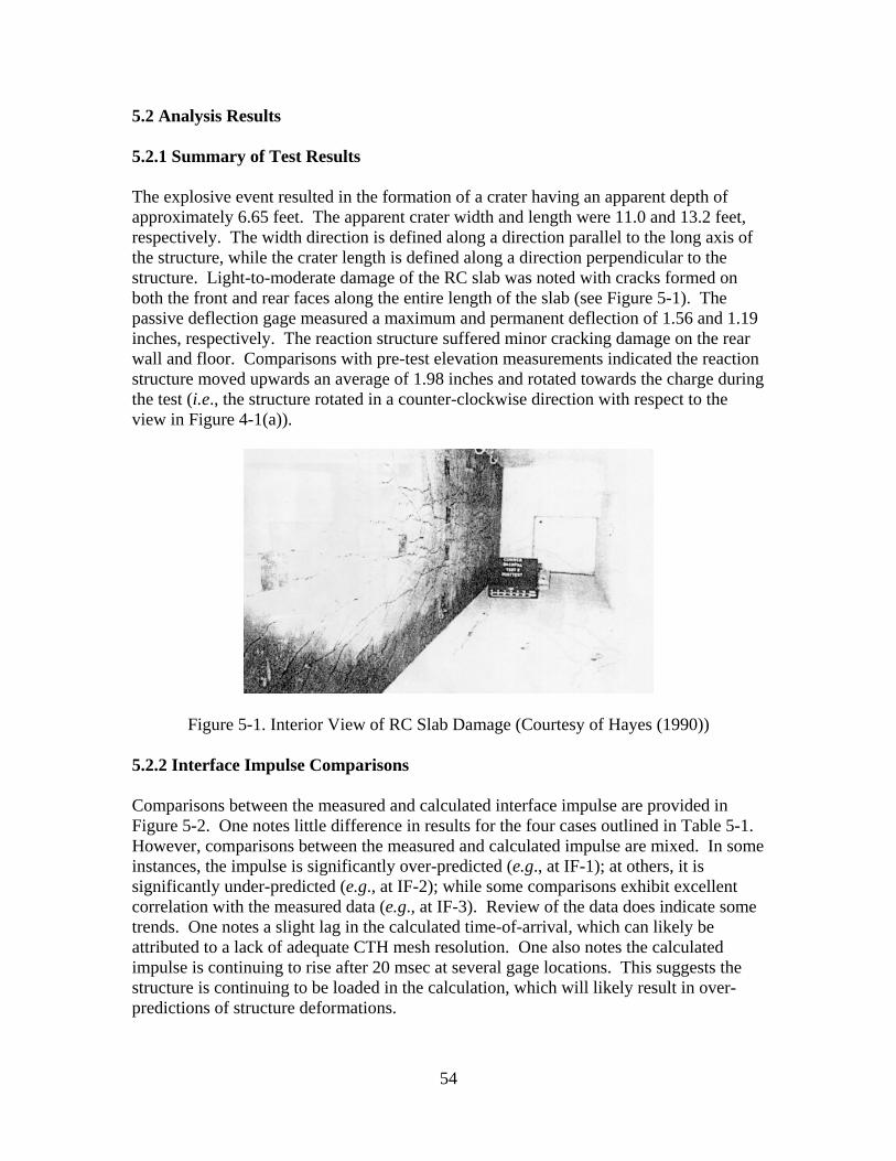
5.2 Analysis Results 5.2.1 Summary of Test Results The explosive event resulted in the formation of a crater having an apparent depth of approximately 6.65 feet. The apparent crater width and length were 11.0 and 13.2 feet, respectively. The width direction is defined along a direction parallel to the long axis of the structure, while the crater length is defined along a direction perpendicular to the structure. Light-to-moderate damage of the RC slab was noted with cracks formed on both the front and rear faces along the entire length of the slab (see Figure 5-1). The passive deflection gage measured a maximum and permanent deflection of 1.56 and 1.19 inches, respectively. The reaction structure suffered minor cracking damage on the rear wall and floor. Comparisons with pre-test elevation measurements indicated the reaction structure moved upwards an average of 1.98 inches and rotated towards the charge during the test (i.e., the structure rotated in a counter-clockwise direction with respect to the view in Figure 4-1(a)).

Figure 5-1. Interior View of RC Slab Damage (Courtesy of Hayes (1990)) 5.2.2 Interface Impulse Comparisons Comparisons between the measured and calculated interface impulse are provided in Figure 5-2. One notes little difference in results for the four cases outlined in Table 5-1. However, comparisons between the measured and calculated impulse are mixed. In some instances, the impulse is significantly over-predicted (e.g., at IF-1); at others, it is significantly under-predicted (e.g., at IF-2); while some comparisons exhibit excellent correlation with the measured data (e.g., at IF-3). Review of the data does indicate some trends. One notes a slight lag in the calculated time-of-arrival, which can likely be attributed to a lack of adequate CTH mesh resolution. One also notes the calculated impulse is continuing to rise after 20 msec at several gage locations. This suggests the structure is continuing to be loaded in the calculation, which will likely result in over-predictions of structure deformations.

54

The impulse comparisons should be used with some discretion. A detailed examination of the impulse history indicates a non-smooth (or jagged) rise in the data. This is readily apparent in the IF-1 and IF-5 data, but is also evident to some degree at the other gage locations. The jaggedness is a consequence of spurious, non-physical oscillations in the pressure data. These oscillations were short-lived, but sufficient to affect the integrated impulse. It is believed the oscillations were the result of tracers moving in and out of mixed material cells (i.e., cells composed of both Eulerian and Lagrangian materials). Attempts were made to avoid this problem by using the CTH noi option with tracers initially located in a cell forward of the structure; however, it is apparent these attempts were unsuccessful. Thus, care should be exercised in the interpretation of the interface impulse results. This problem was encountered in the Test 1 calculation, but to a much lesser degree. It is likely that the increased motion exhibited by the slab in the Test 1 calculation assisted with keeping the tracers in a cell composed only of soil.

55

(a) Gage IF-1 (b) Gage IF-2

(c) Gage IF-3 (d) Gage IF-5

(e) Gage IF-6 (f) Gage IF-8

Figure 5-2. Impulse Comparisons at Interface Gages

56

5.2.3 Structure Response Comparisons Plots depicting the explosive event and structure response at selected times are provided in Figures 5-3 through 5-6. The results presented are for the baseline (v 1.6) case; however, they are typical of those observed for the other three cases. The physics of the event are generally comparable to that noted in Test 1, with the exception that there is significantly less deformation of the RC slab. The thicker slab used in this test results in a much stiffer structure. Consequently, the interface pressures are higher resulting in more loading applied to the structure. In turn, the rigid body velocity of the structure is larger than that observed in Test 1. The slab does deform; however, there is no breach with the calculated damage characterized as moderate-to-heavy (NDRC (1946)). Comparisons of the structure velocities and displacements in the slab are provided in Figures 5-7 and 5-8, respectively. Similar comparisons for the reaction structure are provided in Figures 5-9 and 5-10. The difference in results for the four cases outlined in Table 5-1 is relatively minor, indicating the code modifications did not have a noticeable effect on the results for this benchmark. When drawing comparisons with the measured data, one generally notes good agreement of the peak initial velocity; however, the calculation indicates a sustained velocity for all cases considered. This leads to an over-prediction of the structure motion at later times (after about 7 msec). Comparisons for the reaction structure indicate reasonably good correlation with the measured data for the translational motion (i.e., for AHS-10 and AHS-11); however, there are noticeable differences along the vertical direction with very little structure rotation predicted in the calculation for all four cases. The reasons for the over-predictions in the slab response are unclear. Comparisons for this benchmark are more ambiguous since there was no clear indication from the interface impulse comparisons as to whether the structure loading was over- or under-predicted. For example, gage locations IF-3 and AHS-3 are relatively close to one another, with excellent correlation of the calculated and measured interface impulse noted at this location. However, the motion at AHS-3 is significantly over-predicted. The calculation suggests there is a continued loading on the structure, well past that observed in the test. There are a number of possible explanations for the differences. First, there is a lack of adequate modeling of the soil response. This is a likely contributor as the model parameters were developed from very limited data and were meant only to approximate the soil response. In addition, the CTH mesh resolution may not be sufficient to capture the redistribution of loading on the slab surface. Another possible contributor to the differences lies with the accuracy of the measured data itself. Recall, there was greater confidence in the measured initial peak velocity over the later-time data for the Test 1 event (Baylot (2004)). It is not unknown if this same interpretation of the data applies to this benchmark. Comparisons of the CTH forces applied to the surface of the slab are provided in Figure 5-11. One notes very little difference in results for the four cases, suggesting that the code modifications did not have a noticeable effect on the results for this benchmark.

57

Thus far, the analysis has only addressed the earlier-time blast/structure interaction, i.e., only out to 20 msec which is the extent of the experimental data. The baseline (v 1.6) calculation was run out to 90 msec to assess the later-time structural response. In particular, comparisons were drawn with the measured maximum and permanent displacements at the RC slab center, which were 1.56 and 1.19 inches, respectively. The calculated maximum and permanent slab displacements were 2.8 and 1.4 inches, respectively. These were derived from the nodal history data by taking the relative displacement between the reaction structure and the data at gage location AHS-0. The maximum displacement was reached 29.6 msec into the calculation, after which there was significant recovery of the slab displacement. Review of the nodal history data and deformed mesh plots indicated the 90 msec duration was sufficient for the purposes of determining the permanent displacement. The displacements were slightly over-predicted in the calculation, which is consistent with the over-prediction in slab velocity at later times. 5.3 Summary The findings for this benchmark are summarized as follows: (a) A parameter study was conducted evaluating the Zapotec code updates as well as selection of the maximum allowed number of Lagrangian subcycles. Comparisons of the calculated interface impulse, structure response, and CTH forces for the parameter variations of interest indicate little difference in results. This suggests the code updates and choice of maximum subcycles has little influence on the results for this benchmark. (b) Comparisons for the calculated and measured interface impulse were mixed, with the impulse over-predicted at some locations, under-predicted at others, with good correlation noted at some. However, these results should be interpreted with care since a number of non-physical spurious oscillations were noted in the pressure data. It is believed these oscillations were the result of tracers moving in and out of mixed material cells. (c) In general, there was good correlation with the measured peak velocity for the slab; however, the calculation indicated a tendency to over-predict velocities later in time. This suggests a continued predicted loading on the structure, which was not observed in the test. There are a number of possible explanations for the differences, including a lack of adequate modeling of the soil response, insufficient CTH mesh resolution at the soil/structure interface to capture the redistribution of loading on the slab face, and inaccuracies associated with the experimental data itself. (d) Comparisons for the reaction structure indicate reasonably good correlation with the measured data for the translational motion; however, there are noticeable differences along the vertical direction with very little structure rotation predicted in the calculations.

58

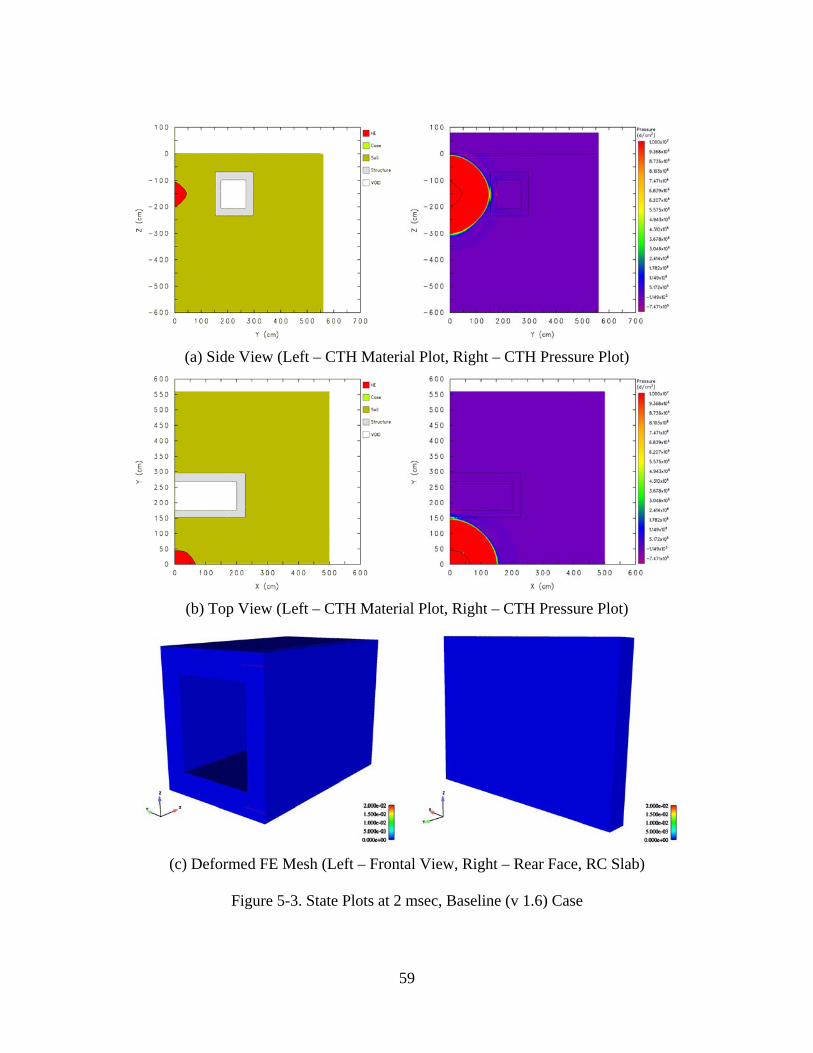
(a) Side View (Left – CTH Material Plot, Right – CTH Pressure Plot)

(b) Top View (Left – CTH Material Plot, Right – CTH Pressure Plot)

(c) Deformed FE Mesh (Left – Frontal View, Right – Rear Face, RC Slab)

Figure 5-3. State Plots at 2 msec, Baseline (v 1.6) Case

59

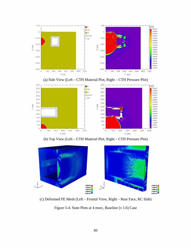
(a) Side View (Left – CTH Material Plot, Right – CTH Pressure Plot)

(b) Top View (Left – CTH Material Plot, Right – CTH Pressure Plot)

(c) Deformed FE Mesh (Left – Frontal View, Right – Rear Face, RC Slab)

Figure 5-4. State Plots at 4 msec, Baseline (v 1.6) Case

60

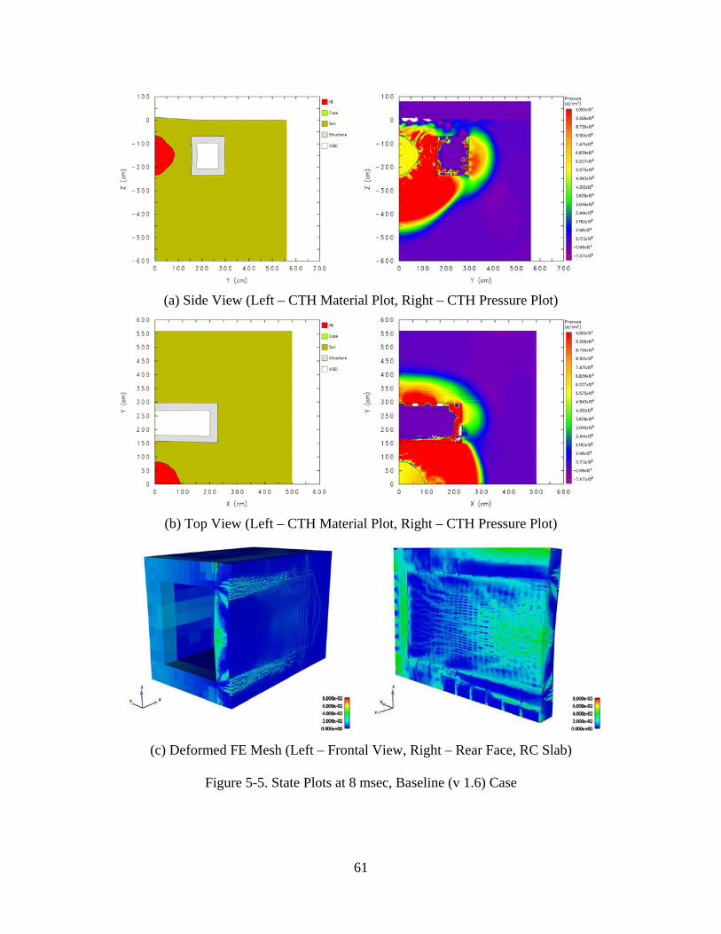
(a) Side View (Left – CTH Material Plot, Right – CTH Pressure Plot)

(b) Top View (Left – CTH Material Plot, Right – CTH Pressure Plot)

(c) Deformed FE Mesh (Left – Frontal View, Right – Rear Face, RC Slab)

Figure 5-5. State Plots at 8 msec, Baseline (v 1.6) Case

61

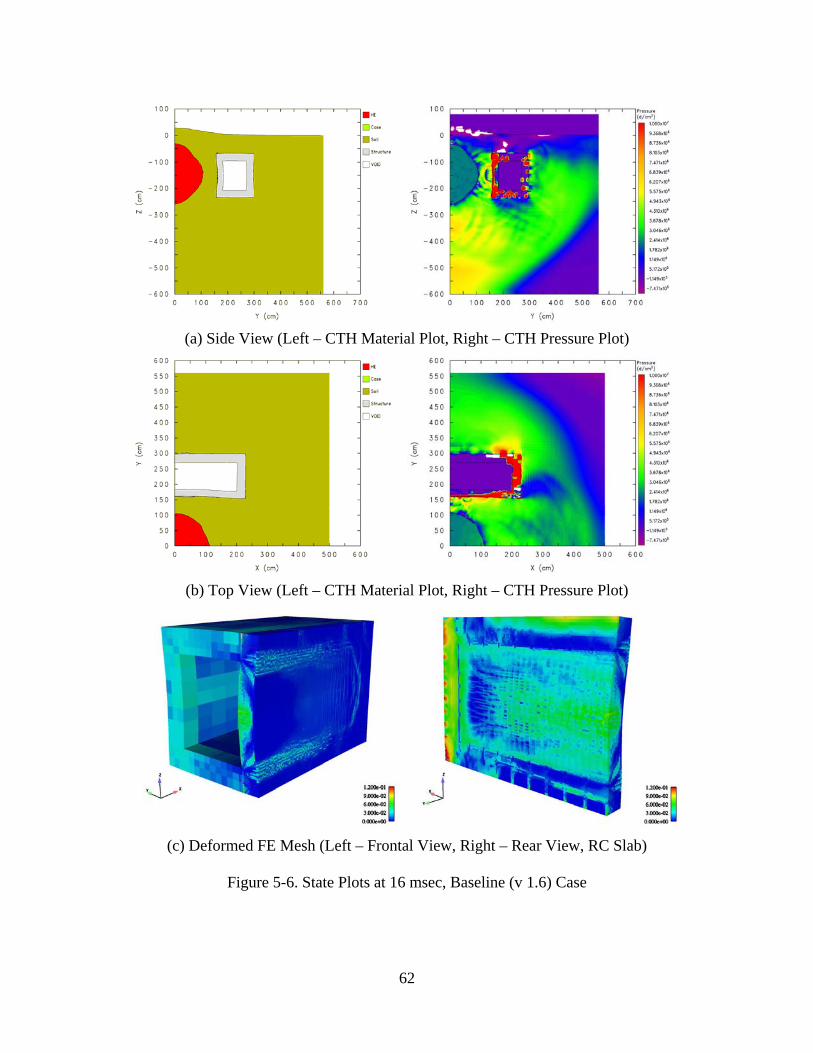
(a) Side View (Left – CTH Material Plot, Right – CTH Pressure Plot)

(b) Top View (Left – CTH Material Plot, Right – CTH Pressure Plot)

(c) Deformed FE Mesh (Left – Frontal View, Right – Rear View, RC Slab)

Figure 5-6. State Plots at 16 msec, Baseline (v 1.6) Case

62

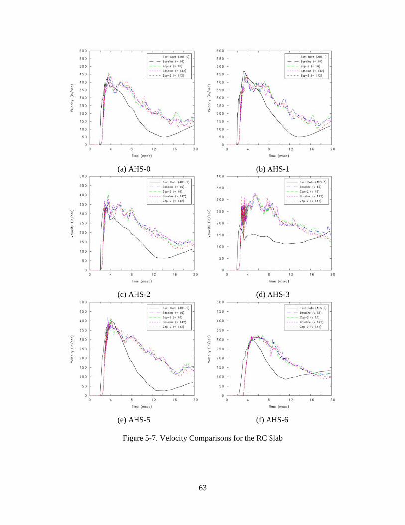
(a) AHS-0 (b) AHS-1

(c) AHS-2 (d) AHS-3

(e) AHS-5 (f) AHS-6

Figure 5-7. Velocity Comparisons for the RC Slab

63

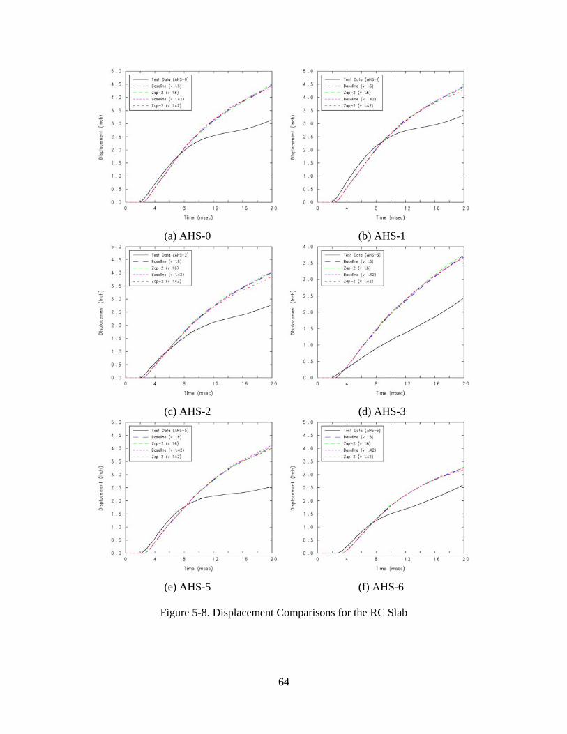
(a) AHS-0 (b) AHS-1

(c) AHS-2 (d) AHS-3

(e) AHS-5 (f) AHS-6

Figure 5-8. Displacement Comparisons for the RC Slab

64

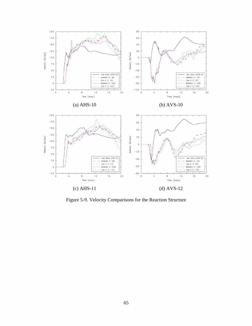
(a) AHS-10 (b) AVS-10

(c) AHS-11 (d) AVS-12

Figure 5-9. Velocity Comparisons for the Reaction Structure

65

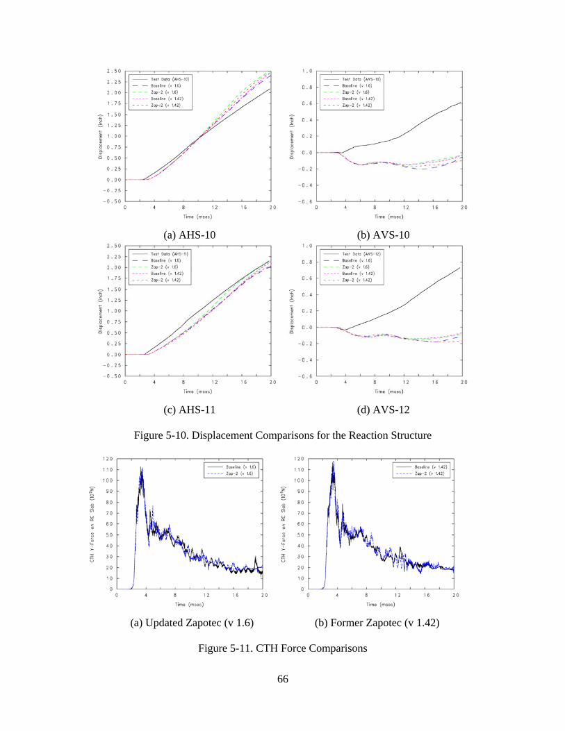
(a) AHS-10 (b) AVS-10

(c) AHS-11 (d) AVS-12

Figure 5-10. Displacement Comparisons for the Reaction Structure

(a) Updated Zapotec (v 1.6) (b) Former Zapotec (v 1.42)

Figure 5-11. CTH Force Comparisons

66

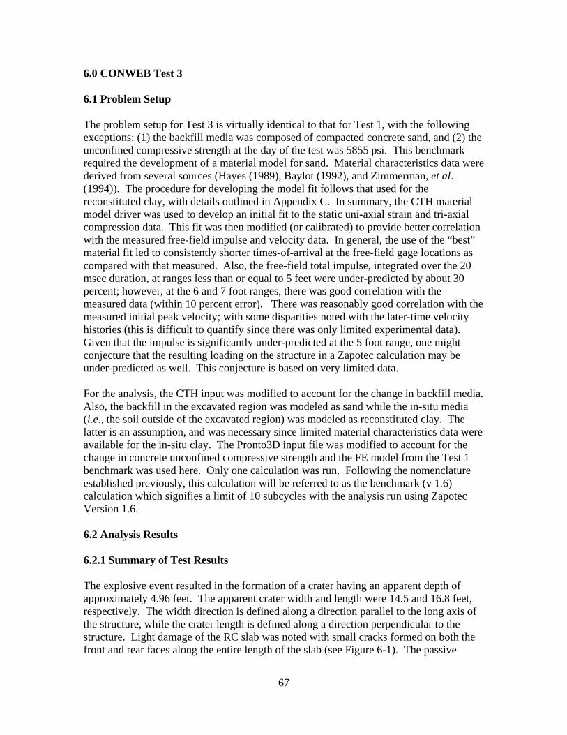
6.0 CONWEB Test 3 6.1 Problem Setup The problem setup for Test 3 is virtually identical to that for Test 1, with the following exceptions: (1) the backfill media was composed of compacted concrete sand, and (2) the unconfined compressive strength at the day of the test was 5855 psi. This benchmark required the development of a material model for sand. Material characteristics data were derived from several sources (Hayes (1989), Baylot (1992), and Zimmerman, et al. (1994)). The procedure for developing the model fit follows that used for the reconstituted clay, with details outlined in Appendix C. In summary, the CTH material model driver was used to develop an initial fit to the static uni-axial strain and tri-axial compression data. This fit was then modified (or calibrated) to provide better correlation with the measured free-field impulse and velocity data. In general, the use of the “best” material fit led to consistently shorter times-of-arrival at the free-field gage locations as compared with that measured. Also, the free-field total impulse, integrated over the 20 msec duration, at ranges less than or equal to 5 feet were under-predicted by about 30 percent; however, at the 6 and 7 foot ranges, there was good correlation with the measured data (within 10 percent error). There was reasonably good correlation with the measured initial peak velocity; with some disparities noted with the later-time velocity histories (this is difficult to quantify since there was only limited experimental data). Given that the impulse is significantly under-predicted at the 5 foot range, one might conjecture that the resulting loading on the structure in a Zapotec calculation may be under-predicted as well. This conjecture is based on very limited data. For the analysis, the CTH input was modified to account for the change in backfill media. Also, the backfill in the excavated region was modeled as sand while the in-situ media (i.e., the soil outside of the excavated region) was modeled as reconstituted clay. The latter is an assumption, and was necessary since limited material characteristics data were available for the in-situ clay. The Pronto3D input file was modified to account for the change in concrete unconfined compressive strength and the FE model from the Test 1 benchmark was used here. Only one calculation was run. Following the nomenclature established previously, this calculation will be referred to as the benchmark (v 1.6) calculation which signifies a limit of 10 subcycles with the analysis run using Zapotec Version 1.6. 6.2 Analysis Results 6.2.1 Summary of Test Results The explosive event resulted in the formation of a crater having an apparent depth of approximately 4.96 feet. The apparent crater width and length were 14.5 and 16.8 feet, respectively. The width direction is defined along a direction parallel to the long axis of the structure, while the crater length is defined along a direction perpendicular to the structure. Light damage of the RC slab was noted with small cracks formed on both the front and rear faces along the entire length of the slab (see Figure 6-1). The passive

67

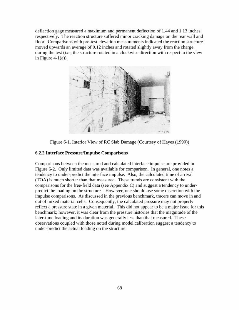
deflection gage measured a maximum and permanent deflection of 1.44 and 1.13 inches, respectively. The reaction structure suffered minor cracking damage on the rear wall and floor. Comparisons with pre-test elevation measurements indicated the reaction structure moved upwards an average of 0.12 inches and rotated slightly away from the charge during the test (i.e., the structure rotated in a clockwise direction with respect to the view in Figure 4-1(a)).

Figure 6-1. Interior View of RC Slab Damage (Courtesy of Hayes (1990)) 6.2.2 Interface Pressure/Impulse Comparisons Comparisons between the measured and calculated interface impulse are provided in Figure 6-2. Only limited data was available for comparison. In general, one notes a tendency to under-predict the interface impulse. Also, the calculated time of arrival (TOA) is much shorter than that measured. These trends are consistent with the comparisons for the free-field data (see Appendix C) and suggest a tendency to under-predict the loading on the structure. However, one should use some discretion with the impulse comparisons. As discussed in the previous benchmark, tracers can move in and out of mixed material cells. Consequently, the calculated pressure may not properly reflect a pressure state in a given material. This did not appear to be a major issue for this benchmark; however, it was clear from the pressure histories that the magnitude of the later-time loading and its duration was generally less than that measured. These observations coupled with those noted during model calibration suggest a tendency to under-predict the actual loading on the structure.

68

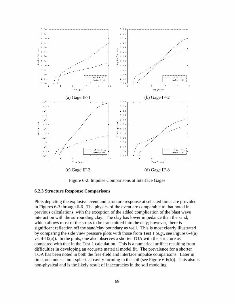
(a) Gage IF-1 (b) Gage IF-2

(c) Gage IF-3 (d) Gage IF-8

Figure 6-2. Impulse Comparisons at Interface Gages

6.2.3 Structure Response Comparisons Plots depicting the explosive event and structure response at selected times are provided in Figures 6-3 through 6-6. The physics of the event are comparable to that noted in previous calculations, with the exception of the added complication of the blast wave interaction with the surrounding clay. The clay has lower impedance than the sand, which allows most of the stress to be transmitted into the clay; however, there is significant reflection off the sand/clay boundary as well. This is most clearly illustrated by comparing the side view pressure plots with those from Test 1 (e.g., see Figure 6-4(a) vs. 4-10(a)). In the plots, one also observes a shorter TOA with the structure as compared with that in the Test 1 calculation. This is a numerical artifact resulting from difficulties in developing an accurate material model fit. The prevalence for a shorter TOA has been noted in both the free-field and interface impulse comparisons. Later in time, one notes a non-spherical cavity forming in the soil (see Figure 6-6(b)). This also is non-physical and is the likely result of inaccuracies in the soil modeling.

69

Comparisons of the structure velocities and displacements in the slab are provided in Figures 6-7 and 6-8, respectively. Similar comparisons for the reaction structure are provided in Figures 6-9 and 6-10. Overall, there is reasonable agreement with the measured peak initial velocities; however, there are notable differences in the later time velocity histories. In general, it appears there is a much faster decay from the initial velocity as compared with that measured. Much better correlation is noted for the displacements. This is not surprising since this is a doubly-integrated quantity. Comparisons for the reaction structure indicate less correlation with the measured data as compared with previous calculations. In particular, there are numerous oscillations in the translational velocity. The reason for these oscillations is unclear, but is likely attributed to mesh effects and/or inaccuracies in the soil modeling. There is much better correlation of the displacement data. The calculation was run out to 60 msec to assess the later-time structural response. The calculated permanent displacement at the slab center was approximately 1.18 inches. This compared well with the measured values of 1.13 inches. The measured maximum displacement was 1.44 inches, which indicates some elastic recovery of the slab. There did not appear to be any recovery of the slab in the calculation (at least over the time duration considered). The accuracy of the calculated loading on the structure is highly dependent on the quality of the constitutive modeling of the soil. The existing model for sand has noted inaccuracies and discretion should be used in interpreting the results (i.e., the comparisons of the maximum displacement are excellent; however, they may have been achieved for the wrong reasons in the calculation). 6.3 Summary The findings for this benchmark are summarized as follows: (a) Developing an accurate material model fit for the sand was problematic. A very coarse model was developed, which was based on the P-alpha EOS and GEO strength model. In particular, problems were encountered with matching both the TOA and pulse width for the free-field pressure data. In turn, this lead to shorter observed TOAs and an under-prediction of the total impulse at close ranges (less than or equal to 5 feet). The inaccuracies in soil modeling were reflected in the calculation, particularly for the interface impulse comparisons. (b) In general, there was good correlation with the measured peak velocity for the slab; however, there were disparities in the later-time velocity histories with a larger velocity decay following the initial peak noted in the calculation. There was reasonably good correlation with the displacements. (c) Comparisons for the reaction structure indicate less correlation with the measured data as compared with previous calculations; however, the comparisons are still within reason. (d) Even with the inaccuracies in the soil modeling, there was still reasonable correlation with the measured data. This is surprising and the reader should take care in interpreting

70

the analysis results, i.e., the right result may have been obtained for the wrong reasons. Further validation of the code is needed, particular for cases involving structures buried in sand. In addition, the use of alternate constitutive models should be explored, especially for sandy soils.

71

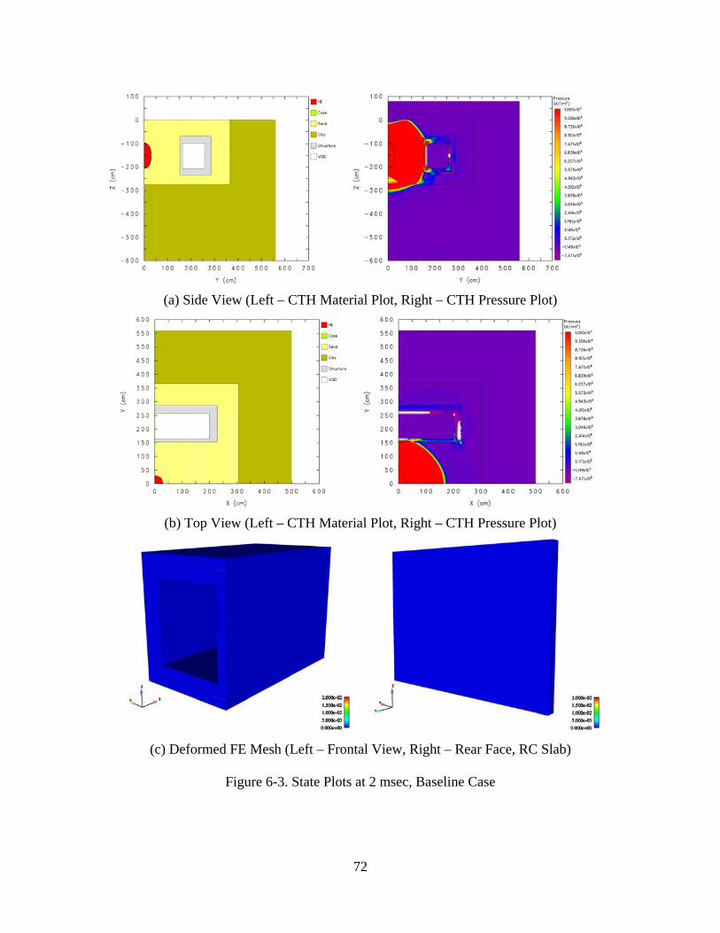
(a) Side View (Left – CTH Material Plot, Right – CTH Pressure Plot)

(b) Top View (Left – CTH Material Plot, Right – CTH Pressure Plot)

(c) Deformed FE Mesh (Left – Frontal View, Right – Rear Face, RC Slab)

Figure 6-3. State Plots at 2 msec, Baseline Case

72

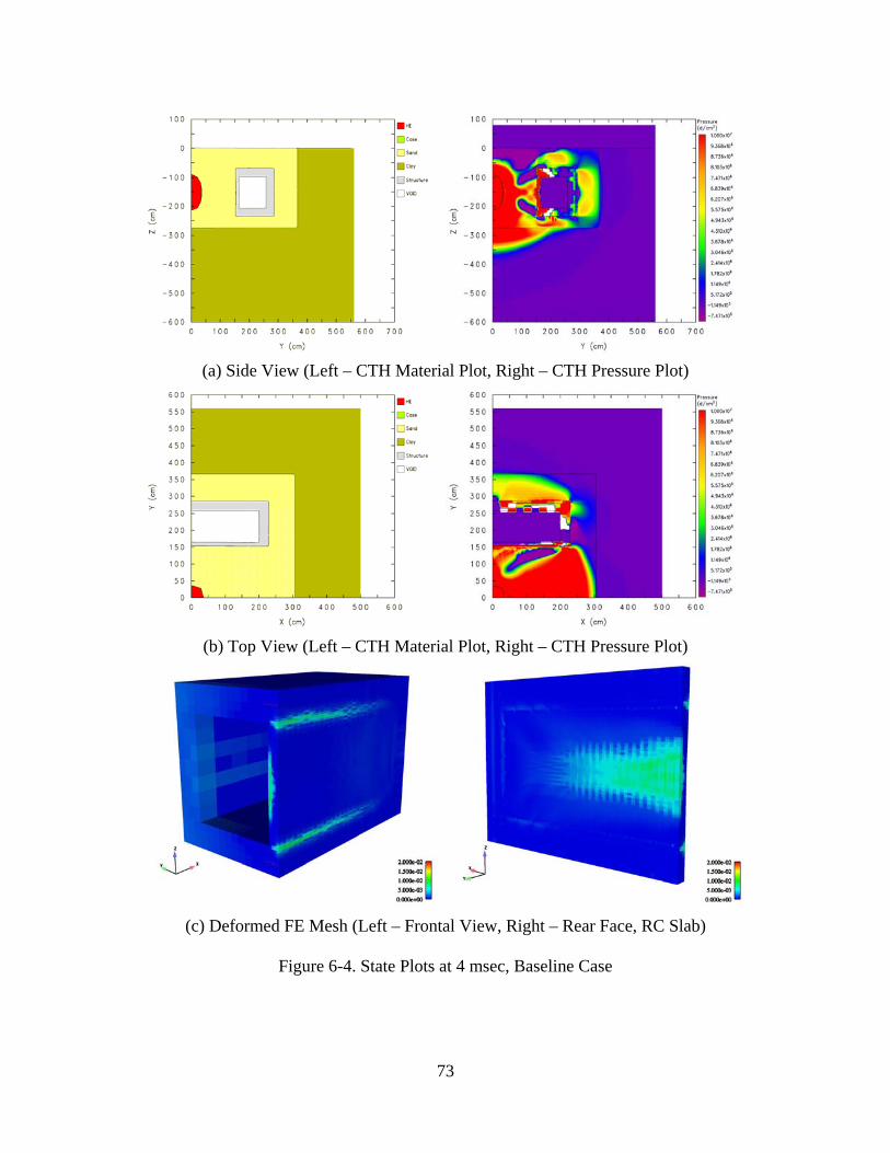
(a) Side View (Left – CTH Material Plot, Right – CTH Pressure Plot)

(b) Top View (Left – CTH Material Plot, Right – CTH Pressure Plot)

(c) Deformed FE Mesh (Left – Frontal View, Right – Rear Face, RC Slab)

Figure 6-4. State Plots at 4 msec, Baseline Case

73

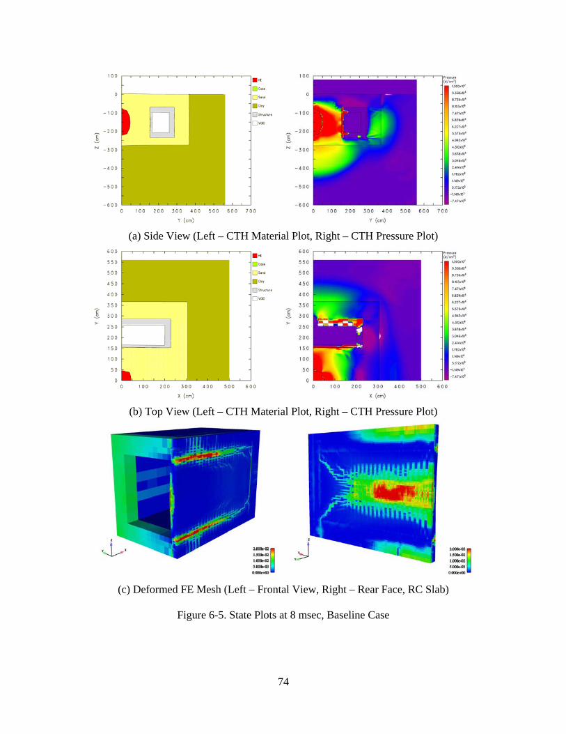
(a) Side View (Left – CTH Material Plot, Right – CTH Pressure Plot)

(b) Top View (Left – CTH Material Plot, Right – CTH Pressure Plot)

(c) Deformed FE Mesh (Left – Frontal View, Right – Rear Face, RC Slab)

Figure 6-5. State Plots at 8 msec, Baseline Case

74

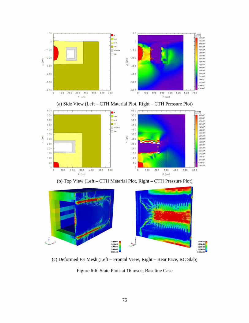
(a) Side View (Left – CTH Material Plot, Right – CTH Pressure Plot)

(b) Top View (Left – CTH Material Plot, Right – CTH Pressure Plot)

(c) Deformed FE Mesh (Left – Frontal View, Right – Rear Face, RC Slab)

Figure 6-6. State Plots at 16 msec, Baseline Case

75

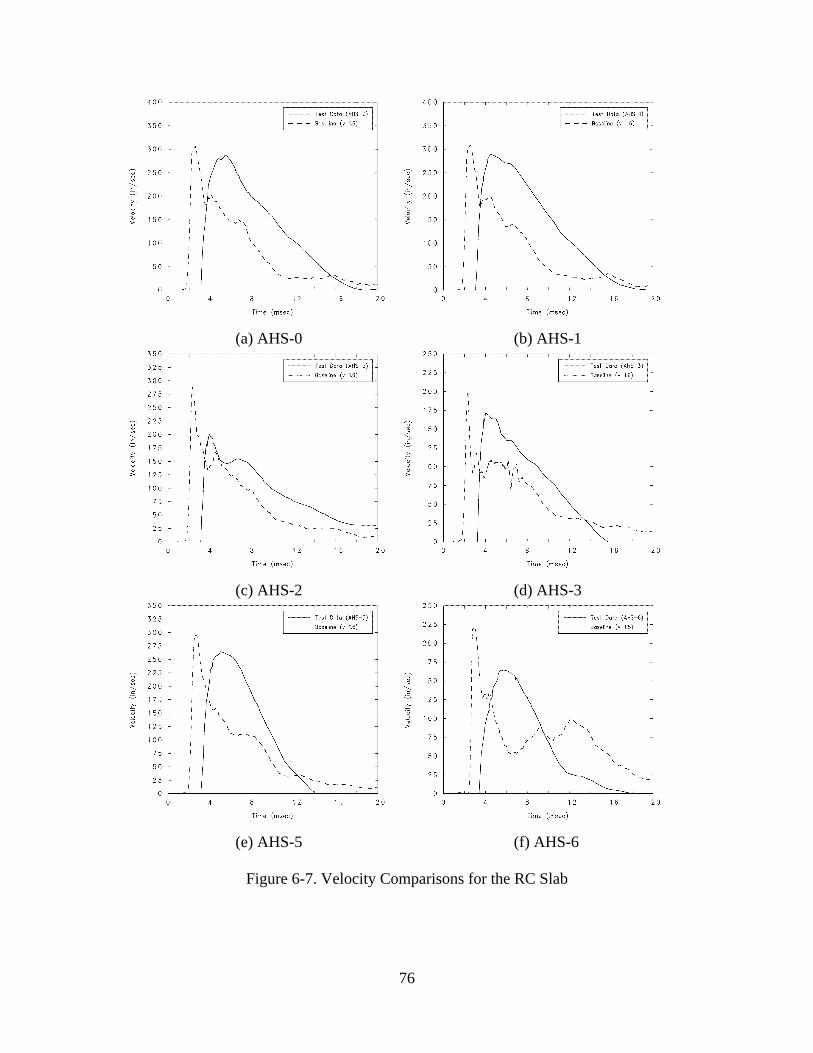
(a) AHS-0 (b) AHS-1

(c) AHS-2 (d) AHS-3

(e) AHS-5 (f) AHS-6

Figure 6-7. Velocity Comparisons for the RC Slab

76

(a) AHS-0 (b) AHS-1

(c) AHS-2 (d) AHS-3

(e) AHS-5 (f) AHS-6

Figure 6-8. Displacement Comparisons for the RC Slab

77

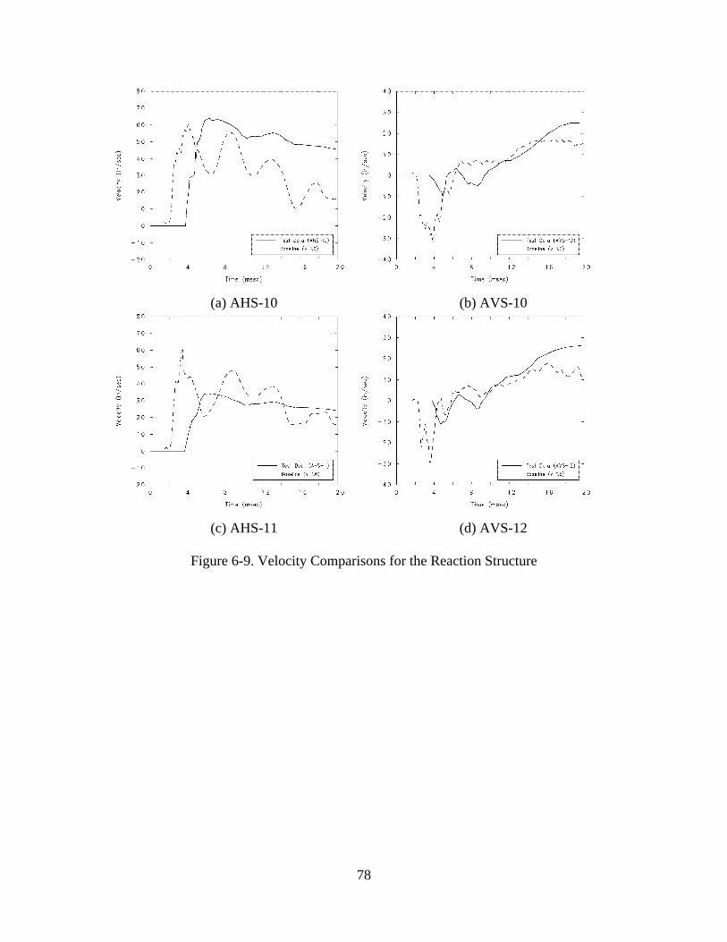
(a) AHS-10 (b) AVS-10

(c) AHS-11 (d) AVS-12

Figure 6-9. Velocity Comparisons for the Reaction Structure

78

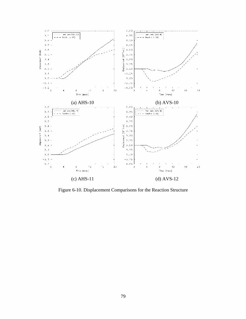
(a) AHS-10 (b) AVS-10

(c) AHS-11 (d) AVS-12

Figure 6-10. Displacement Comparisons for the Reaction Structure

79

7.0 Concluding Remarks For problems involving blast loading on buried structures from close-in detonations, one can, as a minimum, expect significant deformation in the structure. In many situations, the blast impulse will overmatch the structure capacity, resulting in a localized breach as well. The problem is inherently coupled since the structure motion affects the stress state in the neighboring soil, which in turn, affects the loading on the structure. The coupled blast/structure interaction must be taken into account in any numerical modeling of the problem. In this report, the development and application of a coupled Euler-Lagrange (CEL) methodology embedded in the Zapotec code was described. The CEL solution approach is advantageous for modeling blast/structure interaction as it allows flexibility in modeling different portions of the problem using either Eulerian or Lagrangian techniques. As illustrated with the CONWEB benchmarks, the explosive and soil were best modeled as Eulerian as this approach readily handles the shock transmission and large material deformations involved; the RC structure was best modeled using a Lagrangian finite element method since this approach readily allowed for detailed modeling of structure components and their response. The benchmark calculations for the CONWEB tests clearly illustrated the coupled nature of the physical problem. In particular, coupling arose from two sources: (1) interaction arising from the sustained direct blast on the structure, which lead to significant localized wall deformations, and (2) soil/structure interaction arising from rigid body motion of the structure. Although the latter occurs away from the region being directly loaded by the blast, it affects the problem since any rigid body motion of the structure will relieve interface pressures generated by the on-coming blast wave. Both forms of coupling must be accounted for in the numerical solution. The benchmarks illustrated Zapotec’s potential to model blast/structure interaction. These benchmarks also highlighted a number of critical modeling issues. Foremost is the need for accurate modeling of the soil response under blast loading. In this work, material data derived from static laboratory testing was used as a basis for developing a calibrated model which served to approximate the soil response under conditions of blast loading. The calibration utilized experimental data measured at free-field locations opposite the test structure. Relatively simple constitutive models were chosen to replicate the soil response, where the P-alpha EOS was used to model the volumetric response and the Geologic (GEO) model represented the deviatoric response. This combination of models was chosen because (1) there was only limited soil characteristics data to work with, and (2) the models had relatively few input parameters and seemed suited to capturing the soil response. The calibration procedure and choice of constitutive models worked well for Tests 1 and 2, which involved detonations in clay. However, difficulties were encountered during constitutive model calibration for the sand used in Test 3. In particular, the model fit lead to significant under-predictions of the pressure pulse duration as compared with that measured by the free-field soil stress gages. As a result, there was a tendency to under-predict the free-field impulse. One can expect that the interface impulse on the structure

80

was under-predicted as well. In addition, significant disparities in the time-of-arrival (TOA) were noted, where the model resulted in much shorter TOAs as compared with that measured. The sand exhibits both greater porosity and shear strength as compared with the clay. It is apparent that the EOS and strength models chosen to represent the constitutive response for sand were inadequate. There are known limitations for these models (Hertel and Kerley (1998)). These include (1) the material compaction (or current porosity), which is accounted for in the P-alpha EOS, cannot be recovered when the material goes into extension, and (2) the EOS and strength models operate independently. The later is an issue since the change in porosity accounted for in the EOS will have no influence on the material yield. These limitations were recognized prior to the analysis, and it was only expected to be able to grossly represent the soil response. Investigation of other CTH constitutive models suitable for modeling the soil response is needed. In particular, this investigation should focus on models suitable for sandy soils. Concrete constitutive modeling needs to be better addressed too. The existing K&C concrete model is very useful in situations where there is very little material data. This was the case for these benchmarks, where only the unconfined compressive strength was reported. In future benchmarking efforts, detailed concrete characteristics data may be available. Thus, there is a need to better understand the K&C model, which includes understanding the underlying automated procedure for developing internal material parameters as well as the root source for the calibrated model (Recall, the automated model is calibrated to a concrete used in a set of tests conducted at White Sands Missile Range). Although the model implementation is well understood by its developers and has been shown to perform well for selected problems, it has only been fit to a limited set of concrete data. However, there are procedures to update the model should data become available for a different concrete. On a final note, the existing analyses only modeled a portion of the blast/structure interaction problem. This point is best illustrated for the Test 1 benchmark, where the calculation was carried out to the point of incipient breach of the RC slab. The ultimate goal of performing a fully coupled analysis is to assess structure deformation and resulting damage state. The latter is a key issue when addressing collapse of complex structures (e.g., a multi-storied building or a maze of tunnels). Modeling structural failure/breach is going to require using element death within Pronto3D. Element death requires the selection of appropriate death criteria. Traditional deformation-based death criteria, such as those based on equivalent plastic strain or principal strains, are not well suited for capturing the localized breach observed in Test 1. The reason is that there are high concentrations of strain at both the slab center and wall supports. Removal of elements at the supports will lead to over-predictions in slab rotation since the element connectivity is lost at the support. A future goal of Zapotec development is to model structural failure and breach. Consequently, further investigation of the physical damage processes and methods for modeling failure is needed to support this development.

81

8.0 References Summary Technical Report of Division 2, National Defense Research Committee, Volume 1, Effects of Impact and Explosion, Washington D.C. (1946) Attaway, S.W., Mello, F.J., Heinstein, M.W., Swegle, J.W., Ratner, J.A., and Zadoks, R.I., “Pronto3D Users' Instructions: A Transient Dynamic Code for Nonlinear Structural Analysis”, SAND98-1361, Sandia National Laboratories, Albuquerque, NM, June 1998. Attaway, S.W., Matalucci, R.V., Key, S.W., Morrill, K.B., Malvar, L.J., and Crawford, J.E., “Enhancements to Pronto3D to Predict Structural Response to Blast”, SAND2000-1017, Sandia National Laboratories, Albuquerque, NM, May 2000. Baylot, J.T., “Parameters Affecting Loads on Buried Structures Subjected to Localized Blast Effects”, TR-SL-92-9, Waterways Experiment Station, Corps of Engineers, Vicksburg, MS, April 1992. Baylot, J.T., “Loads on Structures Buried in Low-Shear Strength Soils Subjected to Localized Blast Effects”, Ph.D. Dissertation, University of Illinois at Urbana-Champaign (1993). Baylot, J.T., Personal Communication by E-mail, “RE: CONWEB Test 1 Benchmark with Zapotec”, 13 January 2004. Bell, R.L., Baer, M.R., Brannon, R.M., Crawford, D.A., Elrick, M.G., Hertel, E.S., Silling, S.A., and Taylor, P.A., “CTH User’s Manual and Input Instructions, Version 6.0”, Sandia National Laboratories, Albuquerque, NM, November 2000. Bergmann, V.L., “Transient Dynamic Analysis of Plates and Shells with Pronto3D”, SAND91-1182, Sandia National Laboratories, Albuquerque, NM, September 1991. Bessette, G.C., Vaughan, C.T., and Bell, R.L., “Zapotec: A Coupled Euler-Lagrange Code for Modeling Earth Penetration”, Proceedings of the 73rd Shock and Vibration Symposium, Newport RI (2002) Bessette, G.C., Bell, R.L., Cole, R.A., Vaughan, C.T., Yarrington, L., and Attaway, S.W., “Zapotec: A Coupled Eulerian-Lagrangian Computer Code, Methodology and User Manual, Version 1.0”, SAND2003-3097, Sandia National Laboratories, Albuquerque, NM, October 2003. Bessette, G.C., Vaughan, C.T., Bell, R.L., and Attaway, S.W., “Modeling Air Blast on Thin-Shell Structures with Zapotec”, Proceedings of the 74th Shock and Vibration Symposium, San Diego, CA (2003a).

82

Flanagan, D.P., and Belytschko, T., “A Uniform Strain Hexahedron and Quadrilateral with Orthogonal Hourglass Control”, International Journal for Numerical Methods in Engineering, Vol. 17, pp. 679-706 (1981). Hayes, P.G., “Backfill Effects on Response of Buried Reinforced Concrete Slabs”, TR-SL-89-19, Waterways Experiment Station, Corps of Engineers, Vicksburg, MS, September 1989. Hayes, P.G., “Experimental Verification of Theoretical Response Predictions for Buried RC Slabs”, M.S. Thesis, Mississippi State University (1990). Hertel, E.S., Bell, R.L., Elrick, M.G., Farnsworth, A.V., Kerley, G.I., McGlaun, J.M., Petney, S.V., Silling, S.A., Taylor, P.A., and Yarrington, L., “CTH: A Software Family for Multi-Dimensional Shock Physics Analysis”, SAND92-2089C, Sandia National Laboratories, Albuquerque, NM, July 1993. Hertel, E.S., and Kerley, G.I.., “CTH Reference Manual: The Equation of State Package”, SAND98-0947, Sandia National Laboratories, Albuquerque, NM, April 1998. Hollenshead, J.T., Gardner, D.R., and Yarrington, P., Personal Communication, Issues Associated with Modeling the LSG-4 Event, Sandia National Laboratories, March 2004. Key, S.W., Heinstein, M.W., Stone, C.M., Mello, F.J., Blanford, M.L., and Budge, K.G., “A Suitable Low-Order, Eight-Node Tetrahedral Finite Element for Solids”, SAND98-0756, Sandia National Laboratories, Albuquerque, NM, March 1998. Malvar, L.J., Crawford, J.E., Wesevich, J.W., and Simons, D., “A Plasticity Concrete Material Model for DYNA3D”, International Journal of Impact Engineering, Vol. 19, pp. 847-873 (1997). McGlaun, J.M., Thompson, S.L., and Elrick, M.G., “CTH: A Three-Dimensional Shock Wave Physics Code”, International Journal of Impact Engineering, Vol. 10, pp. 351-360 (1990). Silling, S.A., “Coupled Eulerian/Lagrangian Modeling of Penetration”, in: Proceedings of the International Conference on Computational Engineering and Sciences, Los Angeles, CA (2000). Taylor, L.M., and Flanagan, D.P., “Pronto3D, A Three-Dimensional Transient Solid Dynamics Program”, SAND87-1912, Sandia National Laboratories, Albuquerque, NM, March 1989.

83

Zimmerman, H.D., Cooper, G.C., Carney, J.A., Shimano, R.T., and Ito, Y.M., “Calculational Analyses of CONWEB Test Events”, Contract Report SL-94-5, Prepared by the California Research and Technology Division, Titan Corporation, Chatsworth, CA for Waterways Experiment Station, Corps of Engineers, Vicksburg, MS, September 1994.

84

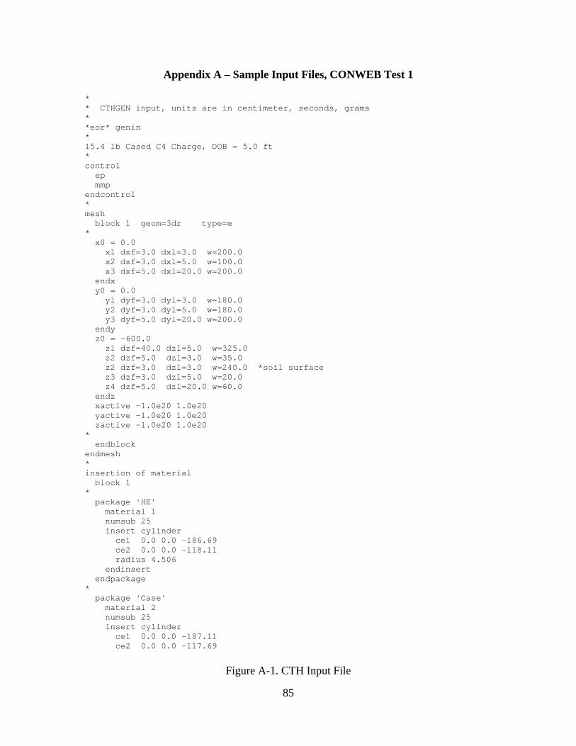
Appendix A – Sample Input Files, CONWEB Test 1 * * CTHGEN input, units are in centimeter, seconds, grams * *eor* genin * 15.4 lb Cased C4 Charge, DOB = 5.0 ft * control ep mmp endcontrol * mesh block 1 geom=3dr type=e * x0 = 0.0 x1 dxf=3.0 dxl=3.0 w=200.0 x2 dxf=3.0 dxl=5.0 w=100.0 x3 dxf=5.0 dxl=20.0 w=200.0 endx y0 = 0.0 y1 dyf=3.0 dyl=3.0 w=180.0 y2 dyf=3.0 dyl=5.0 w=180.0 y3 dyf=5.0 dyl=20.0 w=200.0 endy z0 = -600.0 z1 dzf=40.0 dzl=5.0 w=325.0 z2 dzf=5.0 dzl=3.0 w=35.0 z2 dzf=3.0 dzl=3.0 w=240.0 *soil surface z3 dzf=3.0 dzl=5.0 w=20.0 z4 dzf=5.0 dzl=20.0 w=60.0 endz xactive -1.0e20 1.0e20 yactive -1.0e20 1.0e20 zactive -1.0e20 1.0e20 * endblock endmesh * insertion of material block 1 * package 'HE' material 1 numsub 25 insert cylinder ce1 0.0 0.0 -186.69 ce2 0.0 0.0 -118.11 radius 4.506 endinsert endpackage * package 'Case' material 2 numsub 25 insert cylinder ce1 0.0 0.0 -187.11 ce2 0.0 0.0 -117.69

Figure A-1. CTH Input File

85

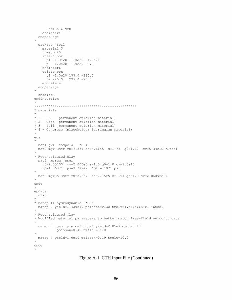
radius 4.928 endinsert endpackage * package 'Soil' material 3 numsub 25 insert box p1 -1.0e20 -1.0e20 -1.0e20 p2 1.0e20 1.0e20 0.0 endinsert delete box p1 -1.0e20 155.0 -230.0 p2 220.0 275.0 -75.0 enddelete endpackage * endblock endinsertion * ************************************************** * materials * * 1 - HE (permanent eulerian material) * 2 - Case (permanent eulerian material) * 3 - Soil (permanent eulerian material) * 4 - Concrete (placeholder lagrangian material) * eos * mat1 jwl compc-4 *C-4 mat2 mgr user r0=7.831 cs=4.61e5 s=1.73 g0=1.67 cv=5.34e10 *Steel * * Reconstituted clay mat3 mgrun user r0=2.05100 cs=2.000e5 s=1.0 g0=1.0 cv=1.0e10 rp=1.96871 ps=7.377e7 *ps = 1071 psi * mat4 mgrun user r0=2.267 cs=2.75e5 s=1.01 go=1.0 cv=2.06896e11 * ende * epdata mix 3 * * matep 1: hydrodynamic *C-4 matep 2 yield=1.430e10 poisson=0.30 tmelt=1.566566E-01 *Steel * * Reconstituted Clay * Modified material parameters to better match free-field velocity data * matep 3 geo yzero=2.303e6 yield=2.05e7 dydp=0.10 poisson=0.45 tmelt = 1.0 * matep 4 yield=1.0e10 poisson=0.19 tmelt=10.0 * ende *

Figure A-1. CTH Input File (Continued)

86

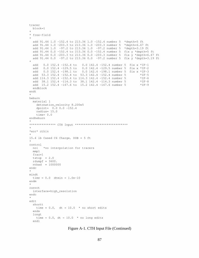
tracer block=1 * * free-field * add 91.44 1.0 -152.4 to 213.36 1.0 -152.4 number 5 *depth=5 ft add 91.44 1.0 -203.3 to 213.36 1.0 -203.3 number 5 *depth=6.67 ft add 91.44 1.0 -97.2 to 213.36 1.0 -97.2 number 5 *depth=3.19 ft add 91.44 0.0 -152.4 to 213.36 0.0 -152.4 number 5 fix y *depth=5 ft add 91.44 0.0 -203.3 to 213.36 0.0 -203.3 number 5 fix y *depth=6.67 ft add 91.44 0.0 -97.2 to 213.36 0.0 -97.2 number 5 fix y *depth=3.19 ft * add 0.0 152.4 -152.4 to 0.0 142.4 -152.4 number 5 fix x *IF-1 add 0.0 152.4 -129.5 to 0.0 142.4 -129.5 number 5 fix x *IF-2 add 0.0 152.4 -198.1 to 0.0 142.4 -198.1 number 5 fix x *IF-3 add 53.3 152.4 -152.4 to 53.3 142.4 -152.4 number 5 *IF-5 add 114.3 152.4 -152.4 to 114.3 142.4 -152.4 number 5 *IF-6 add 38.1 152.4 -114.3 to 38.1 142.4 -114.3 number 5 *IF-8 add 15.2 152.4 -167.6 to 15.2 142.4 -167.6 number 5 *IF-9 endblock endt * heburn material 1 detonation_velocity 8.200e5 dpoint= 0.0 0.0 -152.4 radius= 15.0 time= 0.0 endheburn * *************** CTH Input ****************************** * *eor* cthin * 15.4 lb Cased C4 Charge, DOB = 5 ft * control noi *no interpolation for tracers mmp1 frac=1 tstop = 2.0 rdumpf = 3600. ntbad = 1000000 endc * mindt time = 0.0 dtmin = 1.0e-10 endm * convct interface=high_resolution endc * edit shortt time = 0.0, dt = 10.0 * no short edits ends longt time = 0.0, dt = 10.0 * no long edits endl

Figure A-1. CTH Input File (Continued)

87

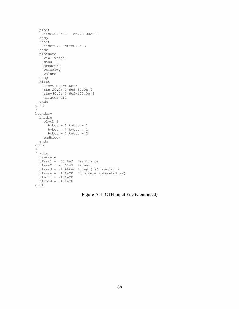
plott time=0.0e-3 dt=20.00e-03 endp restt time=0.0 dt=50.0e-3 endr plotdata vis='vzapa' mass pressure velocity volume endp histt tim=0 dtf=5.0e-6 tim=20.0e-3 dtf=50.0e-6 tim=30.0e-3 dtf=100.0e-6 htracer all endh ende * boundary bhydro block 1 bxbot = 0 bxtop = 1 bybot = 0 bytop = 1 bzbot = 1 bztop = 2 endblock endh endb * fracts pressure pfrac1 = -50.0e9 *explosive pfrac2 = -3.03e9 *steel pfrac3 = -4.606e6 *clay ( 2*cohesion ) pfrac4 = -1.0e20 *concrete (placeholder) pfmix = -1.0e20 pfvoid = -1.0e20 endf

Figure A-1. CTH Input File (Continued)

88

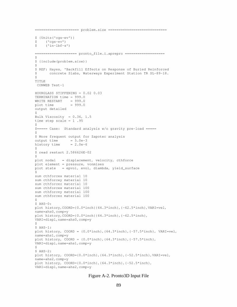
===================== problem.size ============================ $ {Units("cgs-ev")} $ ("cgs-ev") $ ("in-lbf-s") ==================== pronto_file.i.aprepro =================== $ $ {include(problem.size)} $ $ REF: Hayes, "Backfill Effects on Response of Buried Reinforced $ concrete Slabs, Waterways Experiment Station TR SL-89-18. $ TITLE CONWEB Test-1 HOURGLASS STIFFENING = 0.02 0.03 TERMINATION time = 999.0 WRITE RESTART = 999.0 plot time = 999.0 output detailed $ Bulk Viscosity = 0.36, 1.5 time step scale = 1 .95 $ $===== Case: Standard analysis w/o gravity pre-load ===== $ $ More frequent output for Zapotec analysis output time = 5.0e-3 history time = 2.0e-6 $ $ read restart 2.586626E-02 $ plot nodal = displacement, velocity, cthforce plot element = pressure, vonmises plot state = epvol, evol, dlambda, yield_surface $ sum cthforcex material 10 sum cthforcey material 10 sum cthforcez material 10 sum cthforcex material 100 sum cthforcey material 100 sum cthforcez material 100 $ $ AHS-0: plot history,COORD={0.0*inch}{64.3*inch},{-62.5*inch},VARI=vel, name=ahs0,comp=y plot history,COORD={0.0*inch}{64.3*inch},{-62.5*inch}, VARI=displ,name=ahs0,comp=y $ $ AHS-1: plot history, COORD = {0.0*inch},{64.3*inch},{-57.5*inch}, VARI=vel, name=ahs1,comp=y plot history, COORD = {0.0*inch},{64.3*inch},{-57.5*inch}, VARI=displ,name=ahs1,comp=y $ $ AHS-2: plot history, COORD={0.0*inch},{64.3*inch},{-52.5*inch},VARI=vel, name=ahs2,comp=y plot history, COORD={0.0*inch},{64.3*inch},{-52.5*inch}, VARI=displ,name=ahs2,comp=y

Figure A-2. Pronto3D Input File

89

$ $ AHS-3: plot history, COORD = {0.0*inch},{64.3*inch},{-74.5*inch},VARI=vel, name=ahs3,comp=y plot history, COORD = {0.0*inch},{64.3*inch},{-74.5*inch}, VARI=displ,name=ahs3,comp=y $ $ AHS-5: plot history, COORD = {21.0*inch},{64.3*inch},{-57.5*inch},VARI=vel, name=ahs5,comp=y plot history, COORD = {21.0*inch},{64.3*inch},{-57.5*inch}, VARI=displ,name=ahs5,comp=y $ $ AHS-6: plot history, COORD = {45.0*inch},{64.3*inch},{-57.5*inch},VARI=vel, name=ahs6,comp=y plot history, COORD = {45.0*inch},{64.3*inch},{-57.5*inch}, VARI=displ,name=ahs6,comp=y $ $ AHS-10: plot history, COORD = {0.0*inch},{82.3*inch},{-81.5*inch},VARI=vel, name=ahs10,comp=y plot history, COORD = {0.0*inch},{82.3*inch},{-81.5*inch}, VARI=displ,name=ahs10,comp=y $ $ AVS-10: plot history, COORD = {0.0*inch},{82.3*inch},{-81.5*inch},VARI=vel, name=avs10,comp=z plot history, COORD = {0.0*inch},{82.3*inch},{-81.5*inch}, VARI=displ,name=avs10,comp=z $ $ AHS-11: plot history, COORD = {0.0*inch},{94.3*inch},{-81.5*inch},VARI=vel, name=ahs11,comp=y plot history, COORD = {0.0*inch},{94.3*inch},{-81.5*inch}, VARI=displ,name=ahs11,comp=y $ $ AVS-12: plot history, COORD = {0.0*inch},{94.3*inch},{-81.5*inch},VARI=vel, name=avs12,comp=z plot history, COORD = {0.0*inch},{94.3*inch},{-81.5*inch}, VARI=displ,name=avs12,comp=z $ $ Materials $ 10 - concrete slab (hex8) $ 20 - horizontal rebar, temperature steel, 0.133-inch wire (beam) $ 30 - vertical rebar, principal steel, No. 3 (beam) $ 40 - shear steel, 0.195-inch wire (beam) $ 100 - reaction structure (RS), no rebar $ 110 - steel plate on RS, 5/8-inch thick $ 120 - bolts on plane of symmetry $ 130 - bolts not on plane of symmetry $ $ Concrete (matid = 10) $ $ design strength of 5000 psi at 28-days $ 3/8-inch crushed limestone coarse aggregate $ mix used Type II Portland cement $ Average measured strength of L/t=10 slabs at 28-days: 5128 psi $ Strength on day of test: 5855 - 6398 psi (avg ~ 6050 psi) $

Figure A-2. Pronto3D Input File (Continued)

90

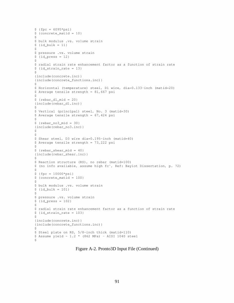
$ {fpc = 6095*psi} $ {concrete_matid = 10} $ $ bulk modulus .vs. volume strain $ {id_bulk = 11} $ $ pressure .vs. volume strain $ {id_press = 12} $ $ radial strain rate enhancement factor as a function of strain rate $ {id_strain_rate = 13} $ {include(concrete.inc)} {include(concrete_functions.inc)} $ $ Horizontal (temperature) steel, D1 wire, dia=0.133-inch (matid=20) $ Average tensile strength = 81,667 psi $ $ {rebar_d1_mid = 20} {include(rebar_d1.inc)} $ $ Vertical (principal) steel, No. 3 (matid=30) $ Average tensile strength = 67,424 psi $ $ {rebar_no3_mid = 30} {include(rebar_no3.inc)} $ $ $ Shear steel, D3 wire dia=0.195-inch (matid=40) $ Average tensile strength = 73,222 psi $ $ {rebar_shear_mid = 40} {include(rebar_shear.inc)} $ $ Reaction structure (RS), no rebar (matid=100) $ (no info available, assume high fc', Ref: Baylot Dissertation, p. 72) $ $ {fpc = 10000*psi} $ {concrete_matid = 100} $ $ bulk modulus .vs. volume strain $ {id_bulk = 101} $ $ pressure .vs. volume strain $ {id_press = 102} $ $ radial strain rate enhancement factor as a function of strain rate $ {id_strain_rate = 103} $ {include(concrete.inc)} {include(concrete_functions.inc)} $ $ Steel plate on RS, 5/8-inch thick (matid=110) $ Assume yield ~ 1.2 * (862 MPa) - AISI 1040 steel $

Figure A-2. Pronto3D Input File (Continued)

91

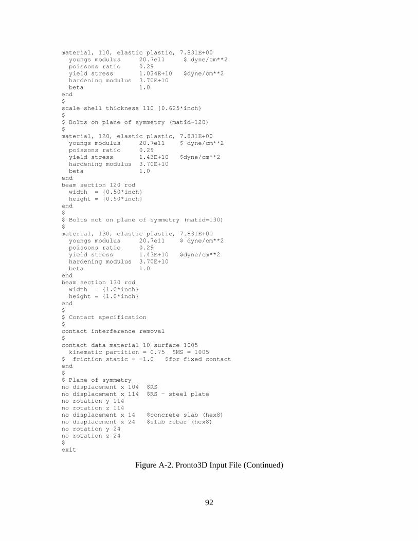
material, 110, elastic plastic, 7.831E+00 youngs modulus 20.7e11 $ dyne/cm**2 poissons ratio 0.29 yield stress 1.034E+10 $dyne/cm**2 hardening modulus 3.70E+10 beta 1.0 end $ scale shell thickness 110 {0.625*inch} $ $ Bolts on plane of symmetry (matid=120) $ material, 120, elastic plastic, 7.831E+00 youngs modulus 20.7e11 $ dyne/cm**2 poissons ratio 0.29 yield stress 1.43E+10 $dyne/cm**2 hardening modulus 3.70E+10 beta 1.0 end beam section 120 rod width = {0.50*inch} height = {0.50*inch} end $ $ Bolts not on plane of symmetry (matid=130) $ material, 130, elastic plastic, 7.831E+00 youngs modulus 20.7e11 $ dyne/cm**2 poissons ratio 0.29 yield stress 1.43E+10 $dyne/cm**2 hardening modulus 3.70E+10 beta 1.0 end beam section 130 rod width = {1.0*inch} height = {1.0*inch} end $ $ Contact specification $ contact interference removal $ contact data material 10 surface 1005 kinematic partition = 0.75 $MS = 1005 $ friction static = -1.0 $for fixed contact end $ $ Plane of symmetry no displacement x 104 $RS no displacement x 114 $RS - steel plate no rotation y 114 no rotation z 114 no displacement x 14 $concrete slab (hex8) no displacement x 24 $slab rebar (hex8) no rotation y 24 no rotation z 24 $ exit

Figure A-2. Pronto3D Input File (Continued)

92

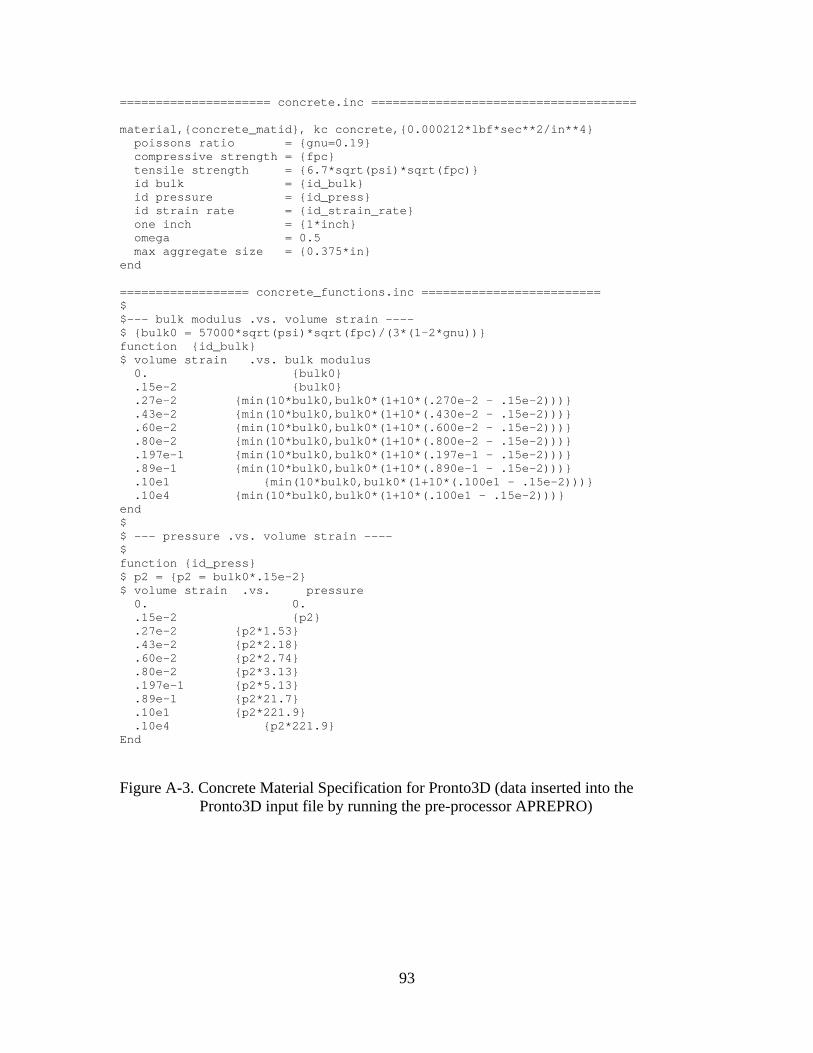
===================== concrete.inc ===================================== material,{concrete_matid}, kc concrete,{0.000212*lbf*sec**2/in**4} poissons ratio = {gnu=0.19} compressive strength = {fpc} tensile strength = {6.7*sqrt(psi)*sqrt(fpc)} id bulk = {id_bulk} id pressure = {id_press} id strain rate = {id_strain_rate} one inch = {1*inch} omega = 0.5 max aggregate size = {0.375*in} end ================== concrete_functions.inc ========================= $ $--- bulk modulus .vs. volume strain ---- $ {bulk0 = 57000*sqrt(psi)*sqrt(fpc)/(3*(1-2*gnu))} function {id_bulk} $ volume strain .vs. bulk modulus 0. {bulk0} .15e-2 {bulk0} .27e-2 {min(10*bulk0,bulk0*(1+10*(.270e-2 - .15e-2)))} .43e-2 {min(10*bulk0,bulk0*(1+10*(.430e-2 - .15e-2)))} .60e-2 {min(10*bulk0,bulk0*(1+10*(.600e-2 - .15e-2)))} .80e-2 {min(10*bulk0,bulk0*(1+10*(.800e-2 - .15e-2)))} .197e-1 {min(10*bulk0,bulk0*(1+10*(.197e-1 - .15e-2)))} .89e-1 {min(10*bulk0,bulk0*(1+10*(.890e-1 - .15e-2)))} .10e1 {min(10*bulk0,bulk0*(1+10*(.100e1 - .15e-2)))} .10e4 {min(10*bulk0,bulk0*(1+10*(.100e1 - .15e-2)))} end $ $ --- pressure .vs. volume strain ---- $ function {id_press} $ p2 = {p2 = bulk0*.15e-2} $ volume strain .vs. pressure 0. 0. .15e-2 {p2} .27e-2 {p2*1.53} .43e-2 {p2*2.18} .60e-2 {p2*2.74} .80e-2 {p2*3.13} .197e-1 {p2*5.13} .89e-1 {p2*21.7} .10e1 {p2*221.9} .10e4 {p2*221.9} End

Figure A-3. Concrete Material Specification for Pronto3D (data inserted into the Pronto3D input file by running the pre-processor APREPRO)

93

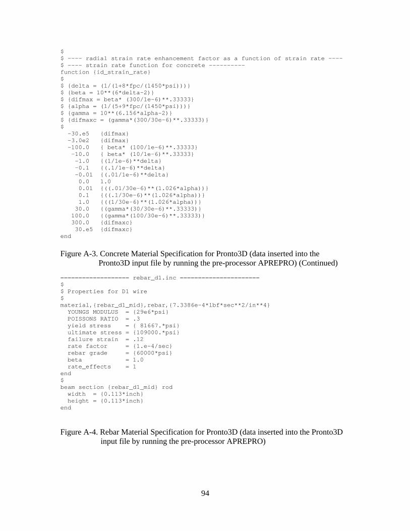
$ $ ---- radial strain rate enhancement factor as a function of strain rate ---- $ ---- strain rate function for concrete ---------- function {id_strain_rate} $ $ {delta = (1/(1+8*fpc/(1450*psi)))} $ {beta = 10**(6*delta-2)} $ {difmax = beta* (300/1e-6)**.33333} $ {alpha = (1/(5+9*fpc/(1450*psi)))} $ {gamma = 10**(6.156*alpha-2)} $ {difmaxc = (gamma*(300/30e-6)**.33333)} $ -30.e5 {difmax} -3.0e2 {difmax} -100.0 { beta* (100/1e-6)**.33333} -10.0 { beta* (10/1e-6)**.33333} -1.0 {(1/1e-6)**delta} -0.1 {(.1/1e-6)**delta} -0.01 {(.01/1e-6)**delta} 0.0 1.0 0.01 {((.01/30e-6)**(1.026*alpha))} 0.1 {((.1/30e-6)**(1.026*alpha))} 1.0 {((1/30e-6)**(1.026*alpha))} 30.0 {(gamma*(30/30e-6)**.33333)} 100.0 {(gamma*(100/30e-6)**.33333)} 300.0 {difmaxc} 30.e5 {difmaxc} end

Figure A-3. Concrete Material Specification for Pronto3D (data inserted into the Pronto3D input file by running the pre-processor APREPRO) (Continued) =================== rebar_d1.inc ====================== $ $ Properties for D1 wire $ material,{rebar_d1_mid},rebar,{7.3386e-4*lbf*sec**2/in**4} YOUNGS MODULUS = {29e6*psi} POISSONS RATIO = .3 yield stress = { 81667.*psi} ultimate stress = {109000.*psi} failure strain = .12 rate factor = {1.e-4/sec} rebar grade = {60000*psi} beta = 1.0 rate_effects = 1 end $ beam section {rebar_d1_mid} rod width = {0.113*inch} height = {0.113*inch} end

Figure A-4. Rebar Material Specification for Pronto3D (data inserted into the Pronto3D input file by running the pre-processor APREPRO)

94

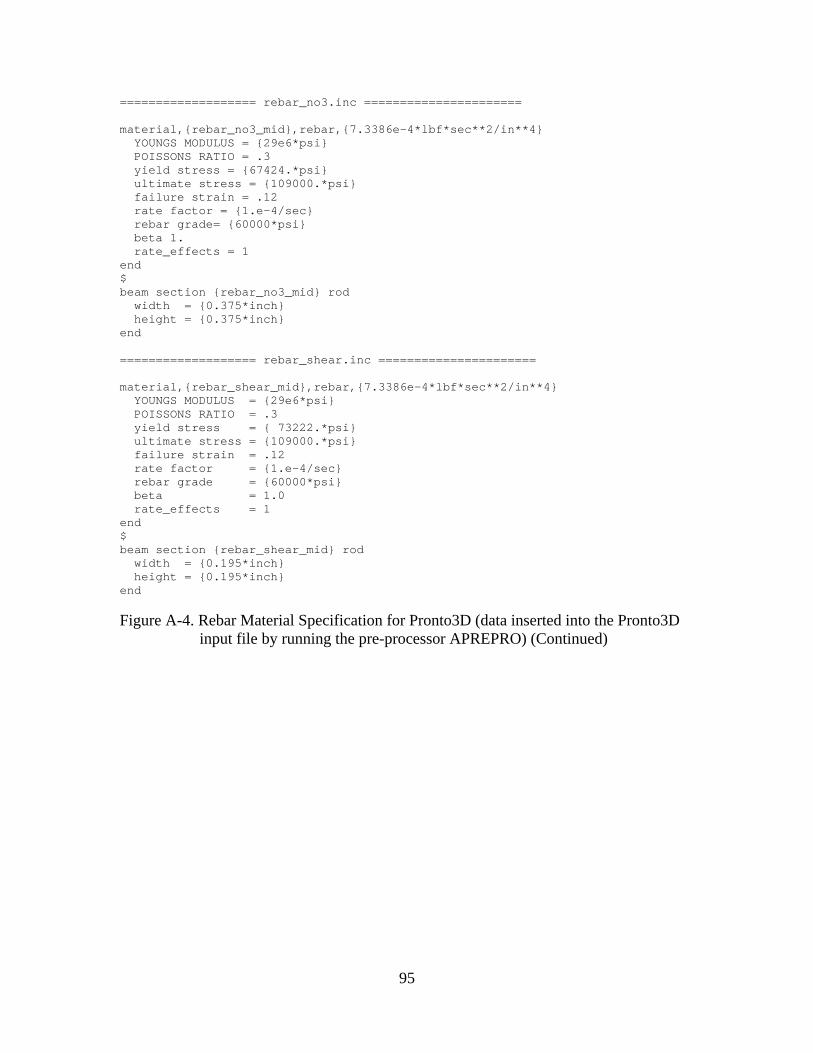
=================== rebar_no3.inc ====================== material,{rebar_no3_mid},rebar,{7.3386e-4*lbf*sec**2/in**4} YOUNGS MODULUS = {29e6*psi} POISSONS RATIO = .3 yield stress = {67424.*psi} ultimate stress = {109000.*psi} failure strain = .12 rate factor = {1.e-4/sec} rebar grade= {60000*psi} beta 1. rate_effects = 1 end $ beam section {rebar_no3_mid} rod width = {0.375*inch} height = {0.375*inch} end =================== rebar_shear.inc ====================== material,{rebar_shear_mid},rebar,{7.3386e-4*lbf*sec**2/in**4} YOUNGS MODULUS = {29e6*psi} POISSONS RATIO = .3 yield stress = { 73222.*psi} ultimate stress = {109000.*psi} failure strain = .12 rate factor = {1.e-4/sec} rebar grade = {60000*psi} beta = 1.0 rate_effects = 1 end $ beam section {rebar_shear_mid} rod width = {0.195*inch} height = {0.195*inch} end

Figure A-4. Rebar Material Specification for Pronto3D (data inserted into the Pronto3D input file by running the pre-processor APREPRO) (Continued)

95

* num_eul = 3 material_map eulerian_material 4 = lagrangian_material 10 *concrete slab eulerian_material 4 = lagrangian_material 100 *reaction structure (RS) eliminate_excess max_subcycles = 10 force material = 10 !concrete slab sideset = 1001, 1002, 1006, 1003 !exterior surface RS option = 2 !forward cell, pressure only * cpu_stop = 8.28e4 !23 hours coupling lag = pronto tcutoff = 40.0e-3 ncutoff = 1000 plot time=2.0e-3 interval=2.00e-03 time=20.0e-3 interval=10.00e-03 restart time=20.0e-3 interval=10.0e-3 time=20.0e-3 interval=20.0e-3 stop_time = 20.0e-3

Figure A-5. Zapotec Input File

96

Appendix B – Development of Material Fit for Reconstituted Clay Material characteristics data for the reconstituted clay were derived from several sources (Hayes (1989), Baylot (1992), Baylot(1993), and Zimmerman, et al. (1994)). Even with a multitude of references, there was limited documentation of the actual uni-axial and tri-axial testing conducted for the soil characterization. The best representation of the response was a material fit depicting the volumetric response and yield envelope, which was reported by Baylot (1992). These fits were reported as a “best fit” to the laboratory data and will form the basis for development of the CTH soil model. For this analysis, the volumetric response of the clay was modeled using a P-alpha equation of state (EOS), while the deviatoric response was modeled using the geologic (GEO) model. The P-alpha model is commonly used to model porous materials, where alpha is a state variable that tracks the crushing of the pores until the fully dense material response is recovered. The GEO model admits a pressure-dependent yield surface. Both models are documented in Bell, et al. (2000). A multi-step approach was taken in the development of the material model. First, the prescribed deformation (PRDEF) option in CTH was utilized to fit model parameters to the material fits depicted in Baylot (1992). Once a reasonable fit was obtained, a series of CTH soil cratering calculations which did not include the test structure were conducted to draw comparisons with the measured free-field data. These comparisons provide an independent means for model validation. As mentioned previously, there was limited soil characteristics data available. Table B-1 provides a summary of data from the site characterization for CONWEB Tests 1 and 2. Care was taken during the backfilling to ensure consistency of the media throughout the test bed. This is evident in the relatively low standard deviations for the density and water content. These data coupled with the material fits from Baylot (1992) served in the development of EOS parameters and description of the yield envelope. The material fits from Baylot (1992) are shown in Figures B-1 and B-2. The general procedure for developing the CTH model parameters is outlined in Figure B-3, with the resulting parameters summarized in Table B-2. A series of 2D axisymmetric and 3D cratering calculations were conducted to validate the model fits. For validation, comparisons were drawn with the impulse and velocity history measured at free-field gage locations residing along the radial axis from the charge center. The CTH mesh was composed of a uniform region encompassing the charge and gage locations. For the 2D axisymmetric calculations, resolutions of 1 and 2 cm in the uniform region were considered. For the 3D calculations, resolutions of 3 and 5 cm in the uniform region were considered. The mesh was graded beyond the uniform region with a grading factor of about eight percent, with the mesh extending well beyond the gage locations to avoid artificial reflection from the mesh boundaries. Absorbing (semi-infinite) boundary conditions were applied along the outer extents of the CTH mesh. Out-flow boundary conditions were applied along the top of the CTH mesh initially in contact with the void. The CTH material library JWL EOS for C-4 was used for the explosive charge, with a programmed burn option and detonation at the charge

97

center assumed. The steel case was modeled as mild steel. Material properties for the explosive and case were outlined in Appendix A. During the course of model validation, obvious disparities were noted between the calculated and measured data when using the initial CTH fit. In general, the free-field impulse and velocities were over-predicted, with the velocities severely over-predicted in a number of cases. The CTH material fit was adjusted to provide better correlation with the measured data. The model adjustment was largely an iterative process, where various EOS and strength model parameters were modified in the 2D axisymmetric calculations to assess the change in results. It was found that changes in the strength model parameters exhibited a first-order effect on the results. With this in mind, the cohesion and ultimate yield in the GEO model were adjusted to add strength to the material. The adjusted model will be referred to as the modified fit, with resultant model parameters defined in Table B-2. Comparisons of the material response using the initial and modified fits with the material fits from Baylot (1992) are provided in Figures B-1 and B-2. Note, there is a significant strength enhancement at higher pressures for the modified fit. One of the major difficulties encountered here was that the yield envelope was specified only for relatively low confining pressures. One can expect increased strength at much higher confining pressures. The increased strength in the modified fit is a best guess, meant only to provide a more reasonable comparison with the measured data. Comparisons of the free-field impulse and velocity for the 2D axisymmetric and 3D CTH calculations are provided in Figures B-4 and B-5. These results are based on use of the modified fit. The Zapotec analysis is three-dimensional. Thus, a goal of these comparisons is to assess the convergence properties of the coarser 3D calculations with that of the finer 2D axisymmetric calculations. One notes good agreement of the impulse data for all ranges, with results at the 7-foot standoff having the largest offset from the fine mesh 2D axisymmetric result. Good correlation of the initial peak velocity is noted for all calculations, with disparities between the 2DC and 3D calculations becoming significant at later times. As an aside, the influence of fracture stress was investigated for the 2D axisymmetric calculations. In these calculations, the effect of varying the fractures stress by an order of magnitude was evaluated (i.e., considering fracture stresses of 4.606e4 and 4.606e7 dyne/cm2). The choice of fracture stress was observed to have a negligible effect on the results. Comparisons of the measured data with the results from the 3D calculation (3 cm resolution) are provided in Figures B-6 and B-7. Results based on both the initial and modified fits are provided in the figures. In general, there is improved correlation with the measured data, especially for the free-field velocity. When evaluating the data, one should place emphasis on comparisons for SE-1 and AHF-1, which are at a range of 5-feet from the charge since these gages are coincident with the location of the test structure.

98

The modified fit provides an improvement, but the data comparisons are still problematic. For example, consider the disparities in impulse and velocity at gage location SE-1. These gages are located at a 5-foot standoff from the charge, but along a different azimuth measured with respect to the normal to the test slab surface. One notes reasonably good correlation of the calculated and measured impulse early in time, but a significant difference in the initial peak velocity. It is possible the differences are due to experimental error. It is also possible the disparity is due to limitations in the P-alpha EOS, where the degree of porosity affects only the volumetric response of the material, i.e., there is no mechanism to tie porosity with the deviatoric response (Hertel and Kerley (1998)). Without additional free-field test data, it is not possible to bound the experimental error. Consequently, it is not possible to further determine the reason for the disparity in results. One should bear in mind the modified fit is only a calibrated model, designed to provide a more reasonable assessment of the loading for a Zapotec calculation.

99

Table B-1. Summary of Test Site Characterization Data for Reconstituted Clay Parameter Test 1 Test 2

Average Wet Density 122.5 +/- 2.0 lb/ft3

(1.962 +/- 0.032 g/cc) 123.7 +/- 1.9 lb/ft3

(1.982 +/- 0.030 g/cc) Average Dry Density 99.4 +/- 2.5 lb/ft3

(1.593 +/- 0.040 g/cc) 100.6 +/- 2.5 lb/ft3

(1.611 +/- 0.04 g/cc) Air Void Content 4.4 +/- 2.45 % 3.7 +/- 2.5 % Water Content 23.3 +/- 2.3 % 23.0 +/- 2.4 % Average Seismic Velocity 1100 ft/sec

(33,526 cm/s) 1100 ft/sec

(33,526 cm/s) Table B-2. Material Model Parameters for the Reconstituted Clay 1

Material Model Model Parameter Initial Fit Modified Fit P-alpha EOS Matrix Material

Density, r0 2.051 g/cc

(128 lbm/ft3) 2.051 g/cc

(128 lbm/ft3) Sound Speed, cs 200,000 cm/s

(6562 ft/s) 200,000 cm/s

(6562 ft/s) Linear Coefficient

of us-up Curve, s 1.0 1.0

Gruneisen Parameter, g0

1.0 1.0

Specific Heat 1.0e10 cm2/s2-eV 1.0e10 cm2/s2-eV Initial Porous

Material Density, rp 1.96871 g/cc

(122.9 lbm/ft3) 1.96871 g/cc

(122.9 lbm/ft3) Compaction

Pressure, ps 7.377e7 dyne/cm2

(1070 psi) 7.377e7 dyne/cm2

(1070 psi) Geologic (GEO) Model

Yield Strength at Zero Pressure, yzero

2.303e5 dyne/cm2

(3.3 psi) 2.303e6 dyne/cm2

(33 psi) Yield Strength,

yield 2.05e6 dyne/cm2

(30 psi) 2.05e7 dyne/cm2

(300 psi) Yield Slope at Zero

Pressure, dydp 0.41 0.10

Poisson’s Ratio 0.45 0.45 Melt Temperature 1.0 eV 1.0 eV Fracture Fracture Pressure 4.606e5 dyne/cm2

(6.6 psi) 4.606e6 dyne/cm2

(66 psi) 1 Data are presented in CGS-eV (centimeter-gram-second-electron volt) as this is the system of units required by CTH; however, selected parameters are also specified in English units for convenience.

100

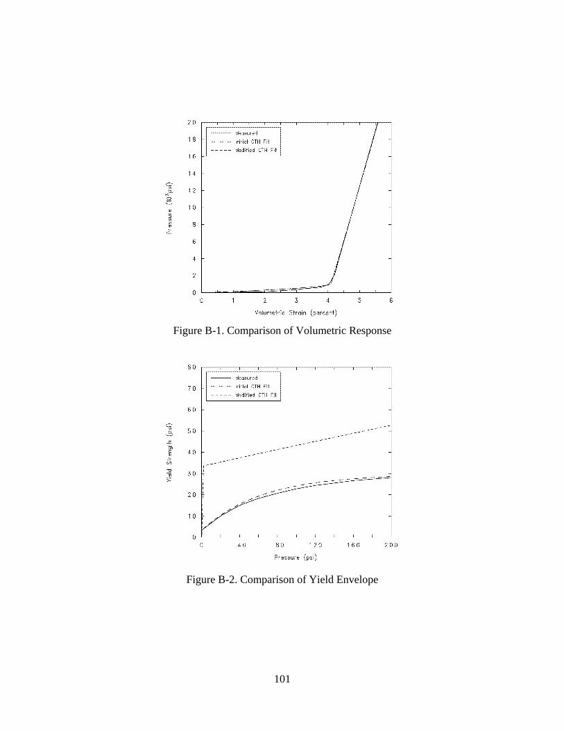
Figure B-1. Comparison of Volumetric Response

Figure B-2. Comparison of Yield Envelope

101

P-alpha EOS Data: (1) Determine the soil matrix density, which is the density at which entrained air is first squeezed out of the soil. This is derived by first determining the volumetric strain at which “lock-up” occurs, which is obtained by extrapolating the linear portion of the hydrostatic stress-strain to the strain axis. The matrix density is computed from the following relation: εv = -η = 1 - ρo / ρ (2) Determine the sound speed co from the following Mie-Gruneisen relation:

p = ρo co2 η / (1 - sη)2

First choose a convenient point on the linear portion of the hydrostatic pressure-strain curve. Determine the pressure and volumetric strain at that point, assuming the slope s of the linear portion of the us-up curve to be 1.0. Then compute the sound speed co. The slope was assumed for lack of data. (3) Assume data for the remaining parameters (Mie-Gruneisen coefficient, g0, and cv). This was necessary due to a lack of Hugoniot data for this material. (4) Iterate to get a best comparison with the published hydrostatic stress-strain curve GEO Model Data: (1) Measure the initial slope at zero pressure, dydp, from the yield envelope (2) Measure the yield strength at large pressures (3) Iterate to get a best comparison with the published yield envelope Fracture Stress: Assume a value twice that of the cohesion. Figure B-3. General Procedure for Developing the CTH Model Parameters

102

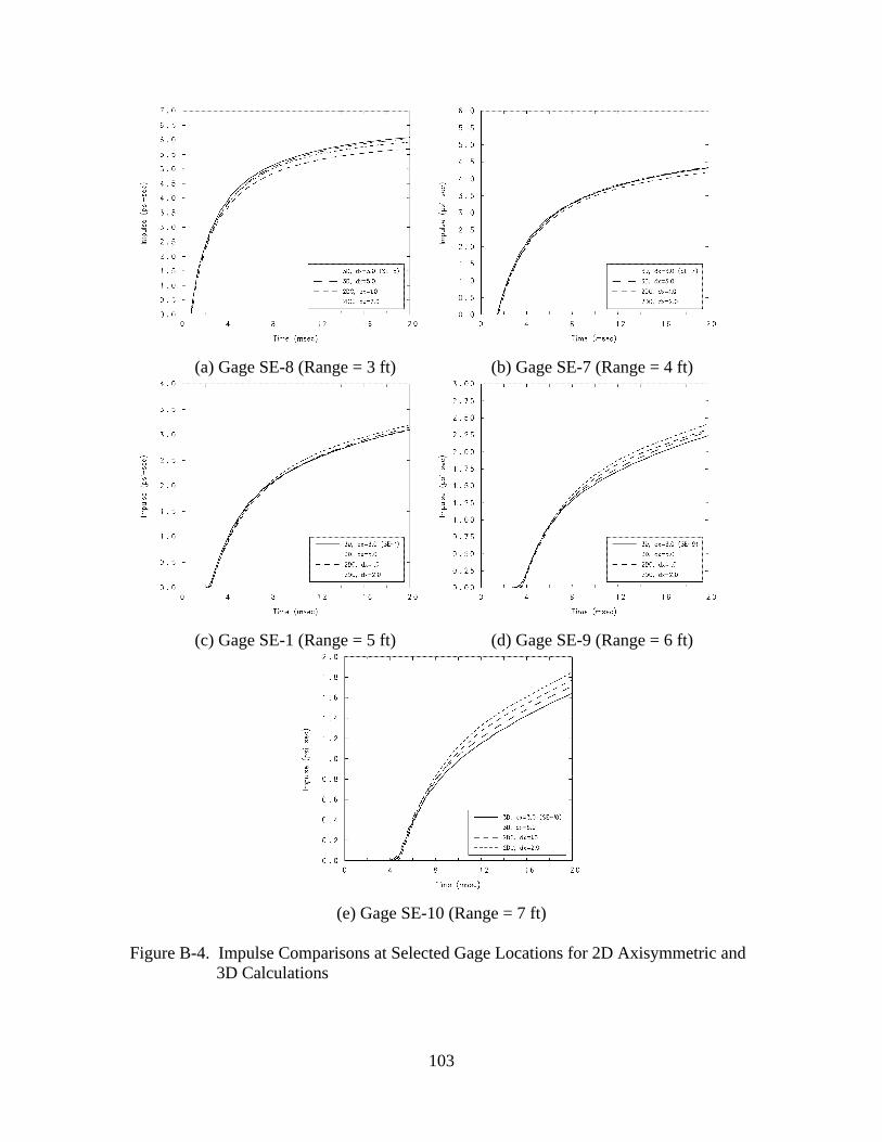
(a) Gage SE-8 (Range = 3 ft) (b) Gage SE-7 (Range = 4 ft)

(c) Gage SE-1 (Range = 5 ft) (d) Gage SE-9 (Range = 6 ft)

(e) Gage SE-10 (Range = 7 ft)

Figure B-4. Impulse Comparisons at Selected Gage Locations for 2D Axisymmetric and 3D Calculations

103

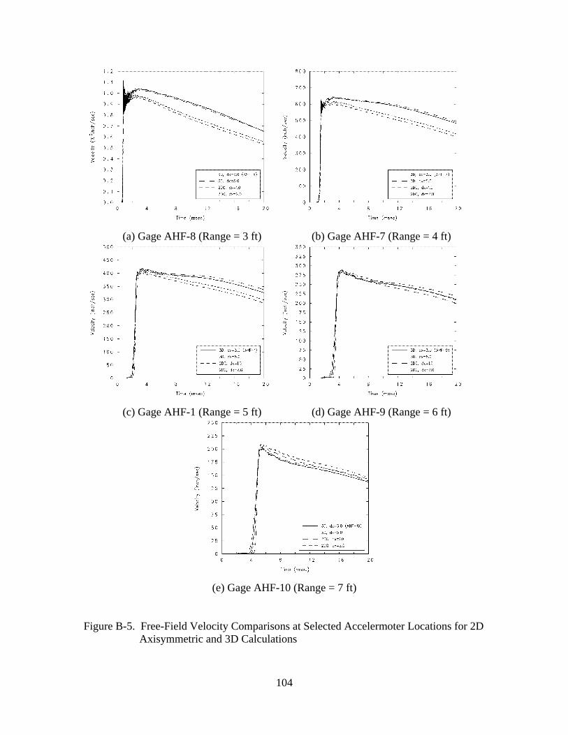
(a) Gage AHF-8 (Range = 3 ft) (b) Gage AHF-7 (Range = 4 ft)

(c) Gage AHF-1 (Range = 5 ft) (d) Gage AHF-9 (Range = 6 ft)

(e) Gage AHF-10 (Range = 7 ft)

Figure B-5. Free-Field Velocity Comparisons at Selected Accelermoter Locations for 2D Axisymmetric and 3D Calculations

104

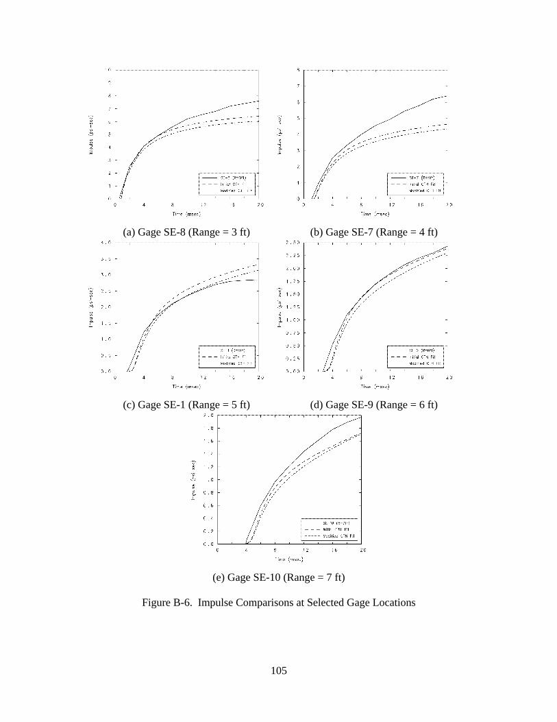
(a) Gage SE-8 (Range = 3 ft) (b) Gage SE-7 (Range = 4 ft)

(c) Gage SE-1 (Range = 5 ft) (d) Gage SE-9 (Range = 6 ft)

(e) Gage SE-10 (Range = 7 ft)

Figure B-6. Impulse Comparisons at Selected Gage Locations

105

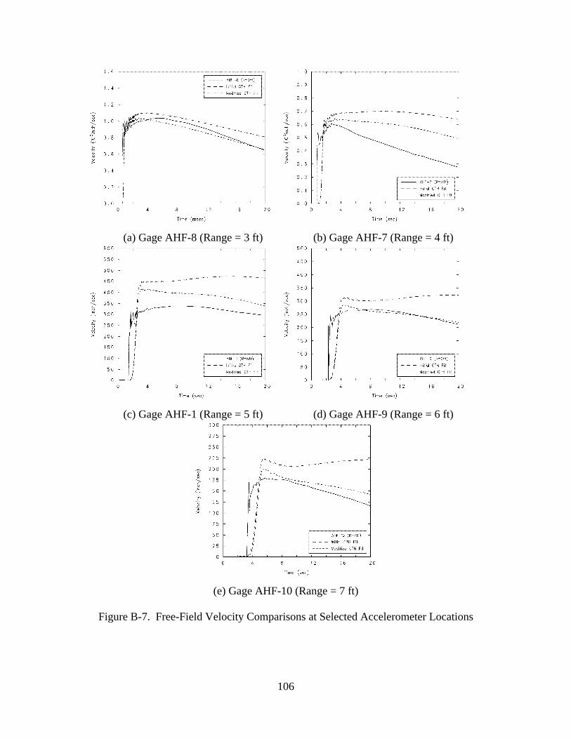
(a) Gage AHF-8 (Range = 3 ft) (b) Gage AHF-7 (Range = 4 ft)

(c) Gage AHF-1 (Range = 5 ft) (d) Gage AHF-9 (Range = 6 ft)

(e) Gage AHF-10 (Range = 7 ft)

Figure B-7. Free-Field Velocity Comparisons at Selected Accelerometer Locations

106

Appendix C – Development of Material Fit for Compacted Concrete Sand Material characteristics data for the compacted concrete sand used in Test 3 were derived from several sources (Hayes (1989), Baylot (1992), and Zimmerman, et al. (1994)). The procedure for developing the model fit follows that used for the reconstituted clay, which was described in Appendix B. As with the clay, the volumetric response of the sand was modeled using a P-alpha equation of state (EOS), while the deviatoric response was modeled using the geologic (GEO) model. The site characterization data from Hayes (1989) is summarized in Table C-1. These data coupled with material fits from Baylot (1992) and Zimmerman, et al. (1994) served in the development of the material model parameters. The material fits are shown in Figures C-1 and C-2. The CTH material model parameters are summarized in Table C-2. Baylot (1992) provides two representations for the volumetric response. The first, defined as Measured-1, was derived from the static tri-axial compression data. The second, defined as Measured-2, is a modification of the initial fit to provide a better replication of the material response in a DYNA3D analysis. The latter fit was used as a basis for the CTH EOS as it too was found to provide better correlation with the measured free-field data. Following the procedure outlined in Appendix B, a series of 2D axisymmetric and 3D cratering calculations were conducted to calibrate the model fits derived using the CTH material driver (i.e., the PRDEF option). Numerous difficulties arose during the course of these analyses. Initially, the ce and pe terms were not included in the P-alpha EOS. This resulted in an extremely “ratty” (and obviously wrong) pressure history. Marlin Kipp (SNL) suggested including the elastic component in the model, which led to much more reasonable results. As previously mentioned, Baylot (1992) provides two fits for the volumetric response. During the course of developing the EOS model inputs, the use of the Measured-2 fit consistently lead to better correlation with the measured free-field peak pressures. Given these observations, the EOS model parameters were adjusted to match the Measured-2 fit. The GEO model allows the user to model the yield envelope as either (1) a non-linear function of the initial slope and cohesion that asymptotes to a prescribed maximum yield, or (2) a linear function with a yield cutoff. For the sand, the later option was chosen. This option is invoked by using a negative value for the initial slope, dydp. The use of the linear fit was found to provide slightly improved correlation with the measured free-field velocities. Comparisons between the measured and calculated free-field impulse are provided in Figure C-3. The calculated results are based on a 3D CTH calculation having a 3 cm resolution. The results from the 2D axisymmetric calculations are not shown, but are comparable. The calculated time of arrival (TOA) is consistently shorter than that measured, with the difference between the two increasing with range from the explosive source. There is also a tendency to under-predict the total impulse at the closer ranges (less than 6 ft), with the error being on the order of 30 percent. Better correlation is noted at the larger standoffs. The under-predicted impulse is a consequence of under-predicting

107

the duration of the pressure pulse (there was excellent correlation with the peak pressures). During the course of model calibration, several attempts were made to increase the pulse width. These attempts included modifying various P-alpha EOS parameter inputs as well as considering a different EOS model. The latter involved developing a fit using the phase-transition (PTRAN), which can be readily adapted to modeling the volumetric response for this material. None of the attempts was successful in increasing the pulse width. Comparisons between the measured and calculated free-field velocities are provided in Figure C-4. The experimental data is limited. Gages AHF-7 and AHF-1 malfunctioned after the initial peak velocity was measured. Also, the measured velocity from AHF-10 is suspect since its history is out-of-character with that measured at other locations (Baylot (1992)). As with the impulse comparisons, one notes a consistently shorter calculated TOA, with the difference between the measured and calculated TOA increasing with range. Discounting gage AHF-10, one observes reasonably good correlation with the measured initial peak velocity, with a tendency to over-predict the peak. There is also a late-time rise in the calculated velocity, which is not evident in the available experimental data. The source of this late-time rise is unknown. In summary, the validation (and calibration) of the model fits for sand have been problematic. Much of the difficulty arose due to the shorter calculated pulse width in the pressure history. This leads to a significant under-prediction of the impulse at near-field gage locations. This is particularly problematic at the 5-foot range, which is coincident with the standoff for the test structure. Given that the impulse is under-predicted at this range, one might surmise that the resulting loading on the structure in a Zapotec calculation may be under-predicted as well.

108

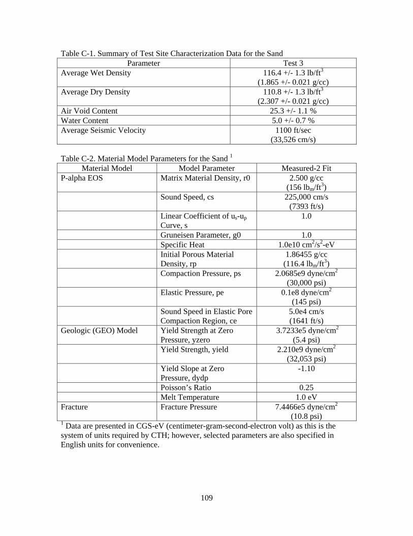
Table C-1. Summary of Test Site Characterization Data for the Sand Parameter Test 3

Average Wet Density 116.4 +/- 1.3 lb/ft3

(1.865 +/- 0.021 g/cc) Average Dry Density 110.8 +/- 1.3 lb/ft3

(2.307 +/- 0.021 g/cc) Air Void Content 25.3 +/- 1.1 % Water Content 5.0 +/- 0.7 % Average Seismic Velocity 1100 ft/sec

(33,526 cm/s) Table C-2. Material Model Parameters for the Sand 1

Material Model Model Parameter Measured-2 Fit P-alpha EOS Matrix Material Density, r0 2.500 g/cc

(156 lbm/ft3) Sound Speed, cs 225,000 cm/s

(7393 ft/s) Linear Coefficient of us-up

Curve, s 1.0

Gruneisen Parameter, g0 1.0 Specific Heat 1.0e10 cm2/s2-eV Initial Porous Material

Density, rp 1.86455 g/cc

(116.4 lbm/ft3) Compaction Pressure, ps 2.0685e9 dyne/cm2

(30,000 psi) Elastic Pressure, pe 0.1e8 dyne/cm2

(145 psi) Sound Speed in Elastic Pore

Compaction Region, ce 5.0e4 cm/s (1641 ft/s)

Geologic (GEO) Model Yield Strength at Zero Pressure, yzero

3.7233e5 dyne/cm2

(5.4 psi) Yield Strength, yield 2.210e9 dyne/cm2

(32,053 psi) Yield Slope at Zero

Pressure, dydp -1.10

Poisson’s Ratio 0.25 Melt Temperature 1.0 eV Fracture Fracture Pressure 7.4466e5 dyne/cm2

(10.8 psi) 1 Data are presented in CGS-eV (centimeter-gram-second-electron volt) as this is the system of units required by CTH; however, selected parameters are also specified in English units for convenience.

109

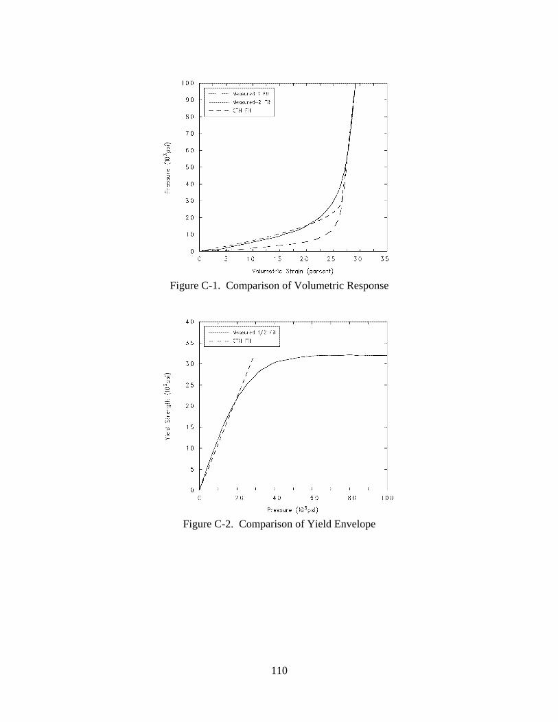
Figure C-1. Comparison of Volumetric Response

Figure C-2. Comparison of Yield Envelope

110

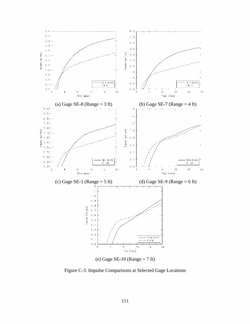
(a) Gage SE-8 (Range = 3 ft) (b) Gage SE-7 (Range = 4 ft)

(c) Gage SE-1 (Range = 5 ft) (d) Gage SE-9 (Range = 6 ft)

(e) Gage SE-10 (Range = 7 ft)

Figure C-3. Impulse Comparisons at Selected Gage Locations

111

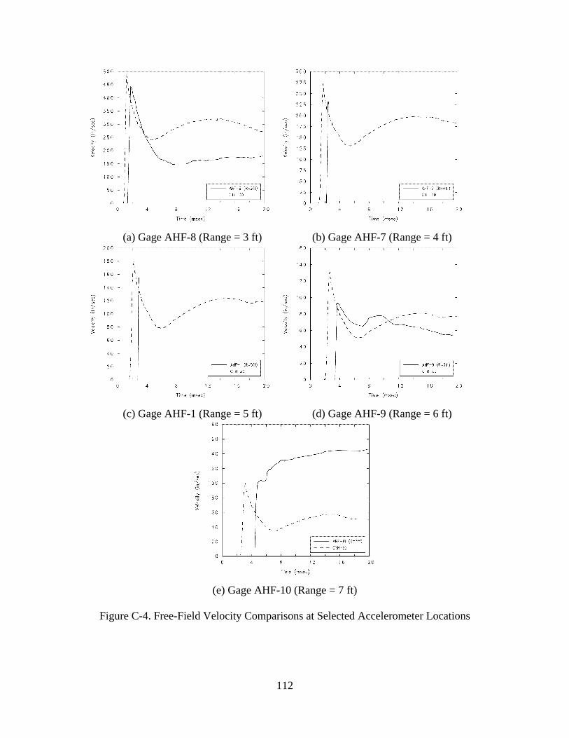
(a) Gage AHF-8 (Range = 3 ft) (b) Gage AHF-7 (Range = 4 ft)

(c) Gage AHF-1 (Range = 5 ft) (d) Gage AHF-9 (Range = 6 ft)

(e) Gage AHF-10 (Range = 7 ft)

Figure C-4. Free-Field Velocity Comparisons at Selected Accelerometer Locations

112

Distribution INTERNAL MS 0899 Technical Library, 9616 (2) MS 9018 Central Technical Files,

8945-1 MS 0316 D. R. Gardner, 9233 MS 0321 W. J. Camp, 9200 MS 0318 P. Yarrington, 9230 MS 0370 M. E. Kipp, 9232 MS 0376 J. G. Arguello, 9126 MS 0378 S. P. Burns, 9231 MS 0378 M. A. Christon, 9231 MS 0378 R. M. Summers, 9231 MS 0378 T. E. Voth, 9231 MS 0378 M. K. Wong, 9231 MS 0378 R. L. Bell, 9232 MS 0378 G. C. Bessette, 9232(6) MS 0378 P. F. Chavez, 9232 MS 0378 R. A. Cole, 9232 MS 0378 S. A. Silling, 9232 MS 0378 P. A. Taylor, 9232 MS 0718 D. J. Ammerman, 6141 MS 0718 J. A. Smith, 6141 MS 0744 V. K. Luk, 6428 MS 0817 S. P. Goudy, 9223 MS 0817 C. T. Vaughan, 9223 MS 0836 D. A. Crawford, 9116 MS 0836 E. S. Hertel, 9116 MS 0847 S. A. Attaway, 9143 MS 9042 J. T. Hollenshead, 8752 EXTERNAL Los Alamos National Laboratory Attn: Roy S. Baty Weapon Systems Engineering Group (Group ESA-WSE) – MS C936 Los Alamos NM 87545 US Nuclear Regulatory Commission Attn: John B. McKirgan 111555 Rockville Pike, Mail Stop T4DS Rockville, MD 20852

US Army Research Laboratory (5) Attn: Dr. Raju Namburu Jerry A. Clarke David J. Grove Stephen Schraml Kent Kimsey Bldg 394, Room 200 Aberdeen Proving Ground, MD 21005 Army Engineer Research and Development Center, Corps of Engineers (5) Waterways Experiment Station Attn: Jimmy Baylot (CEERD-GS-R) Tommy Bevins (CEERD-GS-S) Stephen Akers (CEERD-GS-R) Jim O’Daniel (CEERD-GS-R) Richard Weed (CEERD-IH-C) 3909 Halls Ferry Rd Vicksburg MS 39180-6199 NAWC-WD Attn: Thomas J. Gill 1 Administration Circle Warhead Development Branch Code 478200D China Lake, CA 93555 NSWC Indian Head Division Attn: Sandy Landsberg 101 Strauss Avenue, Bldg 301 Indian Head MD 20640 Air Force Institute of Technology Dept of Aeronautics and Astronautics Attn: Dr. Samir K. Naboulsi 2950 Hobson Way, AFIT/ENY, Bldg 641, Rm 317 Wright-Patterson AFB OH 45433-7765 Applied Research Associates (2) Attn: Terry Caipen Joe Crepeau 4300 San Mateo Blvd NE, Suite A-220 Albuquerque NM 87110 John Prentice 505 Hapgood St Boulder, CO 80302

113

Lockheed Martin Space Systems Company Missile and Space Operations Attn: Erik Matheson 222 Lockheed Martin Way, B157 o/L2-70 Sunnyvale CA 94088-3504 Lockheed Martin Space and Strategic Missiles Attn: Dr. Taft Dehghani 230 Mall Blvd. King of Prussia, PA 19406 Karagozian and Case Attn: Ken Morril 2550 N. Hollywood Way, Suite 500 Burbank CA 91505-5026 Trident Consulting Group Attn: Timothy W. Moore 600 Blvd South, Suite 103 Huntsville AL 35815

114