Czado, Pflüger:

Modeling dependencies between rating categoriesand their effects on prediction in a credit risk portfolio

Sonderforschungsbereich 386, Paper 511 (2006)

Online unter: http://epub.ub.uni-muenchen.de/

Projektpartner

Modeling Dependencies between rating categories

and their effects on prediction in a credit risk

portfolio

Claudia Czado

SCA Zentrum Mathematik

Technische Universitat Munchen, Germany

Carolin Pfluger

Centre for Mathematical Sciences

University of Cambridge, UK

December 13, 2006

Abstract

The internal-ratings based Basel II approach increases the need for the devel-

opment of more realistic default probability models. In this paper we follow the

approach taken in McNeil and Wendin (2006) by constructing generalized linear

mixed models for estimating default probabilities from annual data on companies

with different credit ratings. The models considered, in contrast to McNeil and

Wendin (2006), allow parsimonious parametric models to capture simultaneously

dependencies of the default probabilities on time and credit ratings. Macro-economic

variables can also be included. Estimation of all model parameters are facilitated

with a Bayesian approach using Markov Chain Monte Carlo methods. Special em-

phasis is given to the investigation of predictive capabilities of the models considered.

In particular predictable model specifications are used. The empirical study using

default data from Standard and Poor gives evidence that the correlation between

credit ratings further apart decreases and is higher than the one induced by the

autoregressive time dynamics.

Keywords and phrases: credit risk, default probability, asset correlation, generalized

linear mixed models, Markov chain Monte Carlo, prediction

1

1 INTRODUCTION

The Basel II (2004) agreement allows financial institutions to choose an internal-ratings-

based (IRB) approach to calculate the capital requirement for credit risk. McNeil, Frey,

and Embrechts (2005) provide in Chapter 8 a survey of default probability models used

in credit risk management. In particular threshold and Bernoulli mixture models are

discussed. The risk weight formulas to be used in an IRB Basel II approach can be derived

from a one-factor Gaussian threshold model with preassigned constant asset correlation

(see for example Section 8.4.5 of McNeil et al. (2005)).

However, it has long been known that the value-at-risk and other risk indicators of a credit

portfolio are sensitive to the accuracy of the estimation of default correlations. Since the

data is scarce, it is a challenge to estimate the default correlations among the creditors

correctly. In particular empirical studies have shown that credit default correlations vary

over time (Nickell et al. 2000), rating classes and industry sectors (see Demey et al. (2004),

Servigny and Renault (2003) and Gordy and Heitfield (2002)) and macroe-conomic vari-

ables (Bangia et al. 2002). This empirical evidence of varying default correlations is not

reflected so far in the Basel II approach. McNeil and Wendin (2006) have utilized gen-

eralized linear mixed models (GLMM) to capture these dependencies. As McNeil et al.

(2005) point out on page 403 a GLMM modeling approach allows for flexible models,

which can incorporate macro-economic information as well as dynamic dependence struc-

tures. In contrast to standard industry credit risk models such as Credit Metrics or the

KMV Model, in a GLMM model setup all model parameters are estimated jointly and no

external data sources are needed for model parameters. In particular McNeil and Wendin

(2006) studied Bernoulli mixture models with time dependent random effects. The time

dynamic is modeled through a latent autoregressive component. For their analysis they

used a Bayesian approach applying Markov Chain Monte Carlo (MCMC) techniques to

facilitate parameter estimation and inference in a dynamic setting. This is a very powerful

estimation method since estimation of all parameters is conducted in a single step and

the dependence structure assumed allows to borrow strength for the fit of an area with

scarce data from areas with more information. MCMC methods are summarized in Chib

(2001) and discussed in detail in Gamerman (1997), while many examples are provided in

Gilks, Richardson, and Spiegelhalter (1996). The empirical study presented in McNeil and

Wendin (2006) using Standard & Poor’s data on US firms clearly demonstrated the use-

fulness and potential of their approach. In particular they investigated an unstructured

model for modeling the dependency among default events on rating categories using a

large number of parameters.

We would like to extend their work in two directions: Firstly, it would be interesting to see

2

whether one can use more parsimonious models to uncover the structure of this depen-

dency on rating categories. For instance we would like to analyze whether the dependence

on the rating categories is constant over all categories or whether the dependence decays

for categories with their risk rating further apart. Secondly, for the application of such

models for credit portfolio management it is vital to investigate the usefulness of these

models for prediction.

For the first question we propose to model the joint dynamic over time and rating cate-

gories using a vector autoregressive latent component with different correlation structures

of the error model. This allows us to model different correlation structures among the

rating categories. The model fit of the considered models was assessed using the well es-

tablished deviance information criterion (DIC) of Spiegelhalter et al. (2002) for models

fitted by MCMC techniques in addition to graphical checks.

For the second question we consider models for prediction of one time period which

allows information to be included up to the previous time period. For the macro-economic

variables included in the models this means using a time shifted version of the variable.

In order to compare the predictions we used the Brier-score (Brier 1950), conditional

predictive ordinate (CPO) and standardized predictive residuals proposed by Gelfand

(1996) and also utilized in McNeil and Wendin (2006). Finally we also investigated the

information loss resulting from only using the macro-economic information available up

to the previous year rather than the complete information.

To illustrate our approach we analyze annual data from Standard & Poor’s from 1981 to

2005. As in McNeil and Wendin (2006) we included the Chicago Fed National Activity

Index (CFNAI) as a macro-economic variable to capture the cyclical component of the

systematic risk due to common economic conditions. With regard to prediction our anal-

ysis suggests that the dependence induced by the rating classes decays for rating classes

further apart rather than being constant over all rating classes. When considering predic-

tions using a time shifted CFNAI the model with decaying dependencies shows the best

predictive capability among the models investigated. The information loss from using this

time shifted variable in contrast to the unshifted one was seen not to be severe in this

data set.

2 Bayesian inference for binomial mixed regression

We start with a similar setup as McNeil and Wendin (2006), in particular we assume that

there are K different rating categories and T periods under consideration. Let mtk the

number of firms in category k in time-period t and Mtk the number of defaults in category

3

k in time-period t, t = 1, 2, ..., T , k = 1, 2, . . . , K. One can then consider indicator variables

Ys,t,k such that if in time-period t the sth obligor of rating category k defaults Ys,t,k takes

value 1 and value 0 otherwise. We consider models of the form

(2.1) Mtk |btk ∼ Bin(mtk, g (µk − x′tβ − btk)) independent,

where bt = (bt1, · · · , btK)′ represents the unobserved risk vector in time period t and has

a specified distribution, µ = (µ1, · · · , µK) and β are fixed, unknown parameters, xt is a

p dimensional covariate vector representing observed macro-economic risk factors in time

period t and g(·) is a known link function for binomial data such as the logit or probit

link. In our empirical study we will use the logit link. In the following, we will explore

different distributions for bt, t = 1, · · · , T .

The above model can be motivated as follows: Given bt, the default indicators Ys,t,k are

independent and take value 1 with probability g (µk − x′tβ − btk) and value 0 otherwise.

By defining

(2.2) Vs,t,k = x′tβ + btk + ǫs,t,k

where ǫs,t,k ∼ g i.i.d. we can reformulate the model as follows: The sth obligor in rating

category k defaults in time period t iff Vs,t,k < µk. Vs,t,k can be thought to represent the

asset value of the sth obligor s in rating category k in time-period t and µk can be thought

of as the critical liability as laid out in (Merton 1974). The component x′tβ represents

the asset value attributable to the observed macro-economic market conditions, while

btk is the contribution of rating category k in time period t. The idiosyncratic term ǫs,t,k

captures the contributions which cannot be explained by global or rating category factors.

The implied asset correlation cor (Vs,t,k, Vr,τ,l) is given by

(2.3) cor (Vs,t,k, Vr,τ,l) =cov (bt,k, bτ,l)

√

V ar (bt,k) + ω2√

V ar (bt,k) + ω2,

where V ar (ǫs,t,k) = ω2. For the logit link we have ω2 = π2

3. We see that the distribution

of bt, t = 1, · · · , T can be used to capture different aspects of the default correlations. We

discuss several such choices.

Our baseline model is

bt = (bt, · · · , bt)′, where bt ∼ N(0, σ2) i.i.d. (Model0)

Therefore the layout asset values Vs,t,k and Vr,τ,l are independent for t 6= τ . This assump-

tion clearly is not realistic, because one surely would expect asset values in subsequent

years to be correlated. Furthermore, the correlation of asset values of obligors in the same

time-period always is V ar(bt)V ar(bt)+ω2 , whether or not they are in the same rating category.

4

For the next model we assume asset value correlations are time-dependent but independent

of the rating category. In particular we assume

bt = (bt, · · · , bt)′, where

bt = αbt−1 + σǫt, t = 1, 2, · · · , T (Model1)

b0 = σǫ0/√

1 − α2 with ǫ0, ǫ1, · · · , T i.i.d N(0,1)

This AR(1) time series for bt has a N(0, σ2/(1 − α2)) stationary distribution for |α| < 1.

This model was considered in McNeil and Wendin (2006). The asset values of obligors in

subsequent years are now correlated with cov (bt−1, bt) = σ2/ (1 + α2), t = 1, 2, . . . , T , but

correlations between asset values of obligors in the same time-period are still constant

over rating categories.

The next two models allow for category dependent asset correlations. In Model2 btk is

assumed to be a first order vector autoregressive AR(1) time series with

bt = αbt−1 + ǫt, t = 1, 2, . . . , T

b0 = ǫ0/√

1 − α2

where ǫ0, ǫ1, ... are i.i.d. NK(0, Φ) with

(2.4) Φ =σ2

1 − ρ2

1 ρ . . . ρK−1

ρ 1 . . . ρK−2

......

. . ....

ρK−1 ρK−2 . . . 1

. (Model2)

Here Nn(µ, Σ) denotes a n-dimensional normal distribution with mean vector µ and

covariance matrix Σ. Model2 introduces implied asset correlations

(2.5) cor (Vs,t,k, Vr,τ,l) =Φk,lα

|t−τ |/ (1 − α2)

σ2/ ((1 − α2) (1 − ρ2)) + ω2=

σ2

(1−ρ2)(1−α2)ρ|k−l|α|t−τ |

σ2/ ((1 − α2) (1 − ρ2)) + ω2.

Here the asset values of obligors in the same rating category are most strongly correlated

and the asset values of obligors in similar rating categories are more closely correlated

than those of obligors in disparate rating categories.

The final model considered is similar to Model2, only the covariance matrix Φ is replaced

by

(2.6) Φ =σ2

1 − ρ2

1 ρ . . . ρ

ρ 1 . . . ρ...

.... . .

...

ρ ρ . . . 1

. (Model3)

5

The implied asset correlations for Model3 are

(2.7) cor (Vs,t,k, Vr,τ,l) =Φk,lα

|t−τ |/ (1 − α2)

σ2/ (1 − α2) + ω2=

σ2

(1−ρ2)(1−α2)ρ1(k 6=l)α|t−τ |

σ2/ (1 − α2) + ω2,

where 1(k 6= l) takes the value 1 if k 6= l and 0 otherwise. This model incorporates the

assumption that asset values of obligors in the same rating category are more closely

correlated than those of obligors in different rating categories but for obligors in different

rating categories it does not make a difference whether or not their rating categories are

similar.

To complete the model formulation for a Bayesian setup we have to specify the prior

distributions. As in McNeil and Wendin (2006) we choose non-informative priors for

the parameters and hyperparameters of our models. In all models we chose an or-

dered normal NK (0, τ 2I) distribution as prior for µ with τ = 100, i.e. we require

µ1 > µ2 > µ3 > µ4 > µ5 and the prior distribution then is NK (0, τ 2I) Iµ1>µ2>µ3>µ4>µ5.

The variance σ2 was given an improper prior decaying as 1/x. This corresponds to the lim-

iting case σ2 ∼ InvΓ (η, ν) with η = 0 and ν = 0, where InvΓ (η, ν) denotes the inverse

Gamma distribution with parameters η and ν. The coefficient β was given a N (0, τ 2I)

prior. In Model1, Model2 and Model3, α was given a normal prior with mean 0 and stan-

dard deviation 14

truncated to the interval (−1, 1). This informative prior was chosen to

improve convergence of the Markov Chain and had little influence on the quality of the

estimates. In Model2 and Model3 the parameter ρ was given a uniform prior on (−1, 1).

We used an MCMC algorithm to simulate from the posterior distributions. Our algo-

rithms update parameters one at a time. To simulate from univariate full conditional

distributions, which are only known up to a constant, we apply apply the ARS (Adaptive

Rejection Sampling) and ARMS-algorithms (Gilks (1992), Gilks (1996)). The former is

intended for log-concave densities only, whereas the latter can be applied to a wide range

of univariate densities. Only in one case this ARMS-algorithm was found not to work, and

hence a Metropolis-sampling step had to be employed. For every model 10,000 iterations

were used as a burn-in to give the sampler the opportunity to settle down to equilibrium.

The estimates were based on the following 200,000 iterations. Every 40th iteration was

used so that there was a sample of 5,000 simulations available for analysis. This sub-

sampling frequency was chosen after having considered autocorrelation functions for the

simulated values of the parameters.

For both prediction and estimation, we conducted our analyzes not only using covariate

values from the current year, but also using covariate values from the previous year. This

was done to realistically simulate the situation of predicting default probabilities for the

coming year, when only covariate values of the current year are available.

6

3 Model comparison of fit and predictive power

To assess model fit the complete data was used to estimate the posterior distributions. This

gives estimates of quantiles, median, mean and standard deviation for all parameters for

all models. Credible intervals, which are the Bayesian equivalent to confidence intervals,

are used to assess the significance of parameters.

The deviance information criterion (DIC) introduced by Spiegelhalter et al. (2002) is used

to compare the fit of different models. For a probability model p (y |θ ) with observed data

y = (y1, y2, ..., yn) it is defined as DIC := E [D (θ |y) ]+ pD. The posterior mean deviance

is defined as D (θ) = −2log (l (y |θ )) and corresponds to a Bayesian measure of fit or

adequacy, while the effective number of parameters pD := E [D (θ |y )] − D (E [θ |y ]) is a

measure of model complexity. In the case of a model with no random effects pD gives the

number of parameters. Hence, this score considers both complexity and goodness of fit.

When comparing models the model with smallest DIC is to be preferred.

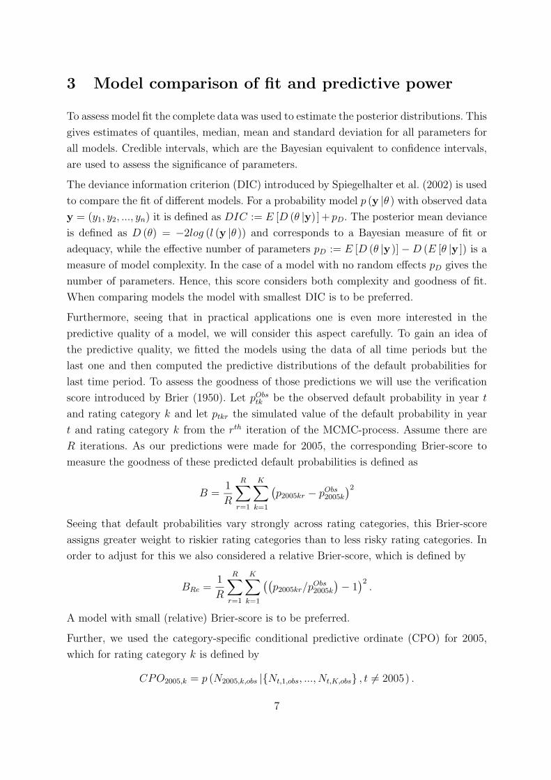
Furthermore, seeing that in practical applications one is even more interested in the

predictive quality of a model, we will consider this aspect carefully. To gain an idea of

the predictive quality, we fitted the models using the data of all time periods but the

last one and then computed the predictive distributions of the default probabilities for

last time period. To assess the goodness of those predictions we will use the verification

score introduced by Brier (1950). Let pObstk be the observed default probability in year t

and rating category k and let ptkr the simulated value of the default probability in year

t and rating category k from the rth iteration of the MCMC-process. Assume there are

R iterations. As our predictions were made for 2005, the corresponding Brier-score to

measure the goodness of these predicted default probabilities is defined as

B =1

R

R∑

r=1

K∑

k=1

(

p2005kr − pObs2005k

)2

Seeing that default probabilities vary strongly across rating categories, this Brier-score

assigns greater weight to riskier rating categories than to less risky rating categories. In

order to adjust for this we also considered a relative Brier-score, which is defined by

BRe =1

R

R∑

r=1

K∑

k=1

((

p2005kr/pObs2005k

)

− 1)2

.

A model with small (relative) Brier-score is to be preferred.

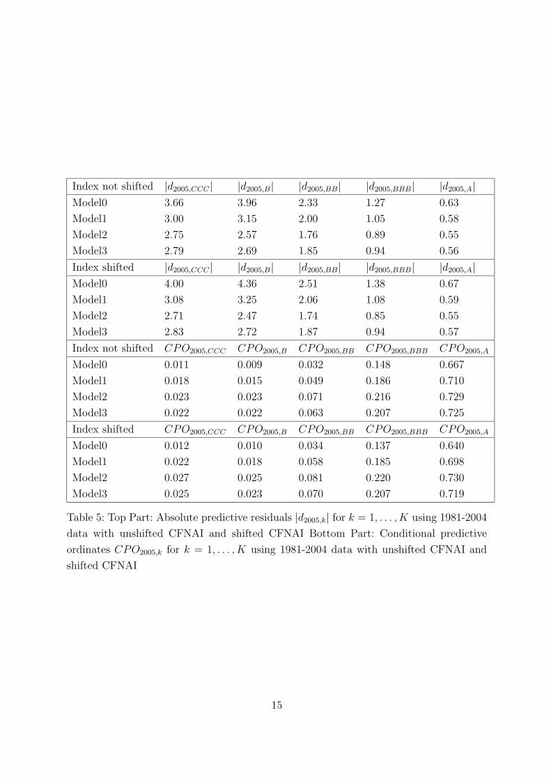
Further, we used the category-specific conditional predictive ordinate (CPO) for 2005,

which for rating category k is defined by

CPO2005,k = p (N2005,k,obs |{Nt,1,obs, ..., Nt,K,obs} , t 6= 2005) .

7

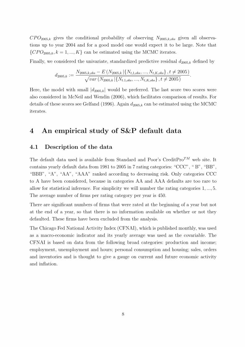
CPO2005,k gives the conditional probability of observing N2005,k,obs given all observa-

tions up to year 2004 and for a good model one would expect it to be large. Note that

{CPO2005,k, k = 1, ..., K} can be estimated using the MCMC iterates.

Finally, we considered the univariate, standardized predictive residual d2005,k defined by

d2005,k :=N2005,k,obs − E (N2005,k |{Nt,1,obs, ..., Nt,K,obs} , t 6= 2005)

√

var (N2005,k |{Nt.1,obs, ..., Nt,K,obs} , t 6= 2005).

Here, the model with small |d2005,k| would be preferred. The last score two scores were

also considered in McNeil and Wendin (2006), which facilitates comparison of results. For

details of these scores see Gelfand (1996). Again d2005,k can be estimated using the MCMC

iterates.

4 An empirical study of S&P default data

4.1 Description of the data

The default data used is available from Standard and Poor’s CreditProTM web site. It

contains yearly default data from 1981 to 2005 in 7 rating categories: “CCC”, “ B”, “BB”,

“BBB”, “A”, “AA”, “AAA” ranked according to decreasing risk. Only categories CCC

to A have been considered, because in categories AA and AAA defaults are too rare to

allow for statistical inference. For simplicity we will number the rating categories 1, ..., 5.

The average number of firms per rating category per year is 450.

There are significant numbers of firms that were rated at the beginning of a year but not

at the end of a year, so that there is no information available on whether or not they

defaulted. These firms have been excluded from the analysis.

The Chicago Fed National Activity Index (CFNAI), which is published monthly, was used

as a macro-economic indicator and its yearly average was used as the covariable. The

CFNAI is based on data from the following broad categories: production and income;

employment, unemployment and hours; personal consumption and housing; sales, orders

and inventories and is thought to give a gauge on current and future economic activity

and inflation.

8

4.2 Results

4.2.1 Estimation and model fit

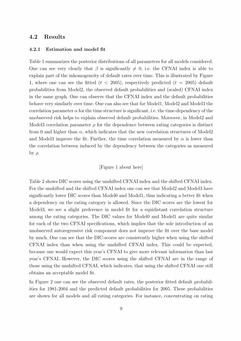
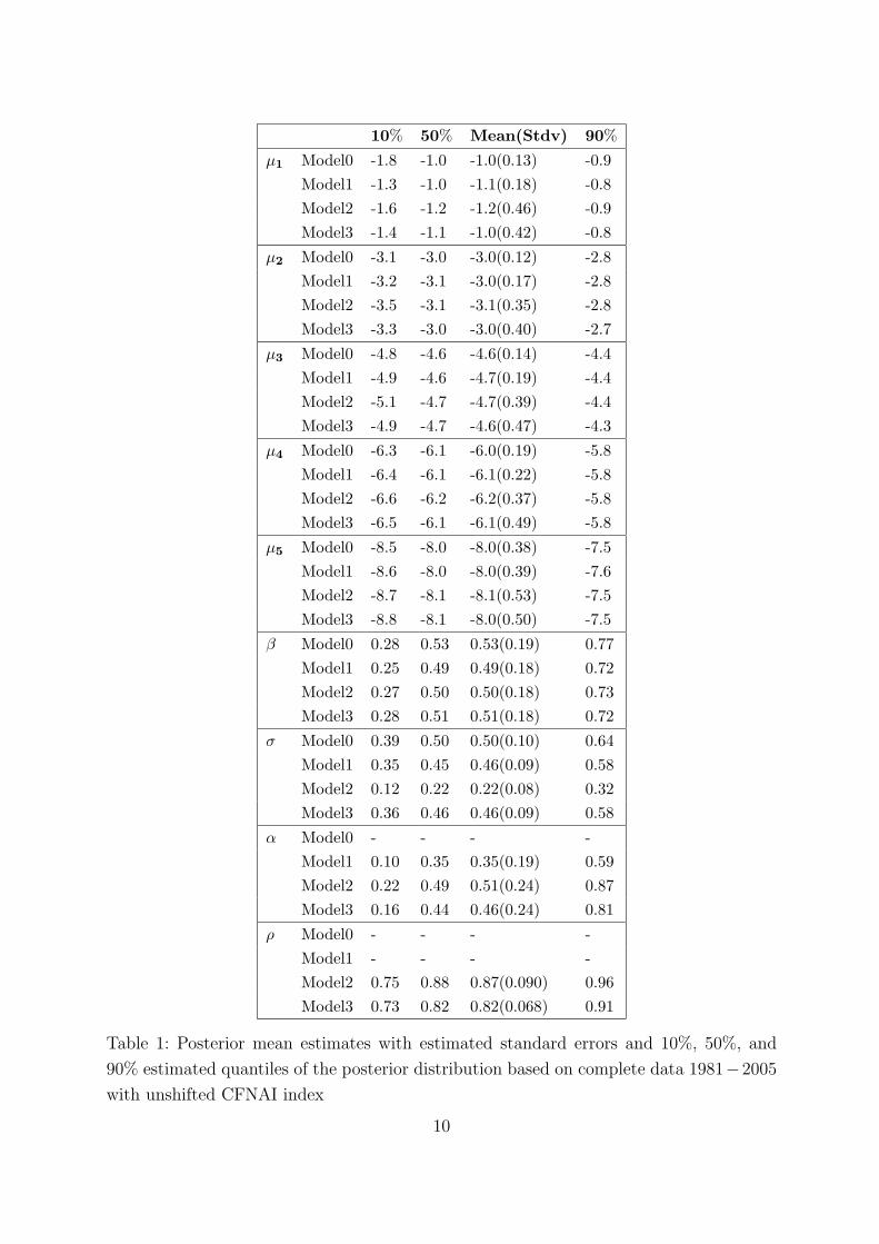
Table 1 summarizes the posterior distributions of all parameters for all models considered.

One can see very clearly that β is significantly 6= 0, i.e. the CFNAI index is able to

explain part of the inhomogeneity of default rates over time. This is illustrated by Figure

1, where one can see the fitted (t < 2005), respectively predicted (t = 2005) default

probabilities from Model2, the observed default probabilities and (scaled) CFNAI index

in the same graph. One can observe that the CFNAI index and the default probabilities

behave very similarly over time. One can also see that for Model1, Model2 and Model3 the

correlation parameter α for the time structure is significant, i.e. the time-dependency of the

unobserved risk helps to explain observed default probabilities. Moreover, in Model2 and

Model3 correlation parameter ρ for the dependence between rating categories is distinct

from 0 and higher than α, which indicates that the new correlation structures of Model2

and Model3 improve the fit. Further, the time correlation measured by α is lower than

the correlation between induced by the dependency between the categories as measured

by ρ.

[Figure 1 about here]

Table 2 shows DIC scores using the unshifted CFNAI index and the shifted CFNAI index.

For the unshifted and the shifted CFNAI index one can see that Model2 and Model3 have

significantly lower DIC scores than Model0 and Model1, thus indicating a better fit when

a dependency on the rating category is allowed. Since the DIC scores are the lowest for

Model3, we see a slight preference in model fit for a equidistant correlation structure

among the rating categories. The DIC values for Model0 and Model1 are quite similar

for each of the two CFNAI specifications, which implies that the sole introduction of an

unobserved autoregressive risk component does not improve the fit over the base model

by much. One can see that the DIC-scores are consistently higher when using the shifted

CFNAI index than when using the unshifted CFNAI index. This could be expected,

because one would expect this year’s CFNAI to give more relevant information than last

year’s CFNAI. However, the DIC scores using the shifted CFNAI are in the range of

those using the unshifted CFNAI, which indicates, that using the shifted CFNAI one still

obtains an acceptable model fit.

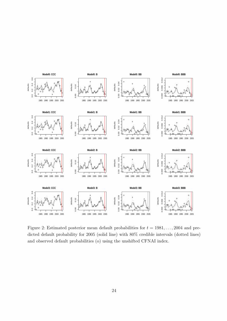
In Figure 2 one can see the observed default rates, the posterior fitted default probabil-

ities for 1981-2004 and the predicted default probabilities for 2005. These probabilities

are shown for all models and all rating categories. For instance, concentrating on rating

9

10% 50% Mean(Stdv) 90%

µ1 Model0 -1.8 -1.0 -1.0(0.13) -0.9

Model1 -1.3 -1.0 -1.1(0.18) -0.8

Model2 -1.6 -1.2 -1.2(0.46) -0.9

Model3 -1.4 -1.1 -1.0(0.42) -0.8

µ2 Model0 -3.1 -3.0 -3.0(0.12) -2.8

Model1 -3.2 -3.1 -3.0(0.17) -2.8

Model2 -3.5 -3.1 -3.1(0.35) -2.8

Model3 -3.3 -3.0 -3.0(0.40) -2.7

µ3 Model0 -4.8 -4.6 -4.6(0.14) -4.4

Model1 -4.9 -4.6 -4.7(0.19) -4.4

Model2 -5.1 -4.7 -4.7(0.39) -4.4

Model3 -4.9 -4.7 -4.6(0.47) -4.3

µ4 Model0 -6.3 -6.1 -6.0(0.19) -5.8

Model1 -6.4 -6.1 -6.1(0.22) -5.8

Model2 -6.6 -6.2 -6.2(0.37) -5.8

Model3 -6.5 -6.1 -6.1(0.49) -5.8

µ5 Model0 -8.5 -8.0 -8.0(0.38) -7.5

Model1 -8.6 -8.0 -8.0(0.39) -7.6

Model2 -8.7 -8.1 -8.1(0.53) -7.5

Model3 -8.8 -8.1 -8.0(0.50) -7.5

β Model0 0.28 0.53 0.53(0.19) 0.77

Model1 0.25 0.49 0.49(0.18) 0.72

Model2 0.27 0.50 0.50(0.18) 0.73

Model3 0.28 0.51 0.51(0.18) 0.72

σ Model0 0.39 0.50 0.50(0.10) 0.64

Model1 0.35 0.45 0.46(0.09) 0.58

Model2 0.12 0.22 0.22(0.08) 0.32

Model3 0.36 0.46 0.46(0.09) 0.58

α Model0 - - - -

Model1 0.10 0.35 0.35(0.19) 0.59

Model2 0.22 0.49 0.51(0.24) 0.87

Model3 0.16 0.44 0.46(0.24) 0.81

ρ Model0 - - - -

Model1 - - - -

Model2 0.75 0.88 0.87(0.090) 0.96

Model3 0.73 0.82 0.82(0.068) 0.91

Table 1: Posterior mean estimates with estimated standard errors and 10%, 50%, and

90% estimated quantiles of the posterior distribution based on complete data 1981−2005

with unshifted CFNAI index

10

Index not shifted DIC Effective # of parameters

Model0 7827.04 25.81

Model1 7826.28 24.93

Model2 7818.11 38.42

Model3 7816.40 38.64

Index shifted DIC Effective # of parameters

Model0 8102.44 26.23

Model1 8102.68 25.94

Model2 8096.70 38.86

Model3 8094.83 41.52

Table 2: DIC score to assess model fit for the considered models. Models are fitted with

data 1981-2005 using unshifted CFNAI (top) and shifted CFNAI (bottom)

category B and the year 1990 one can see that whereas for Model0 and Model1 the ob-

served default probability is not in the fitted 80% credible interval it is in this interval for

Model2 and Model3. One can also see that the fitted expected default probability 1990

is clearly closer to observed default probability 1990 for Model2 and Model3. This again

illustrates the improved fit of Model2 and Model3.

[Figure 2 about here]

From a model fit perspective Model3 is slightly preferrable over Model2. This result has

to be critically examined by checking the predictive capabilities of the models, since this

is the primary interest of the data analyst.

4.2.2 Analysis of predictive distributions

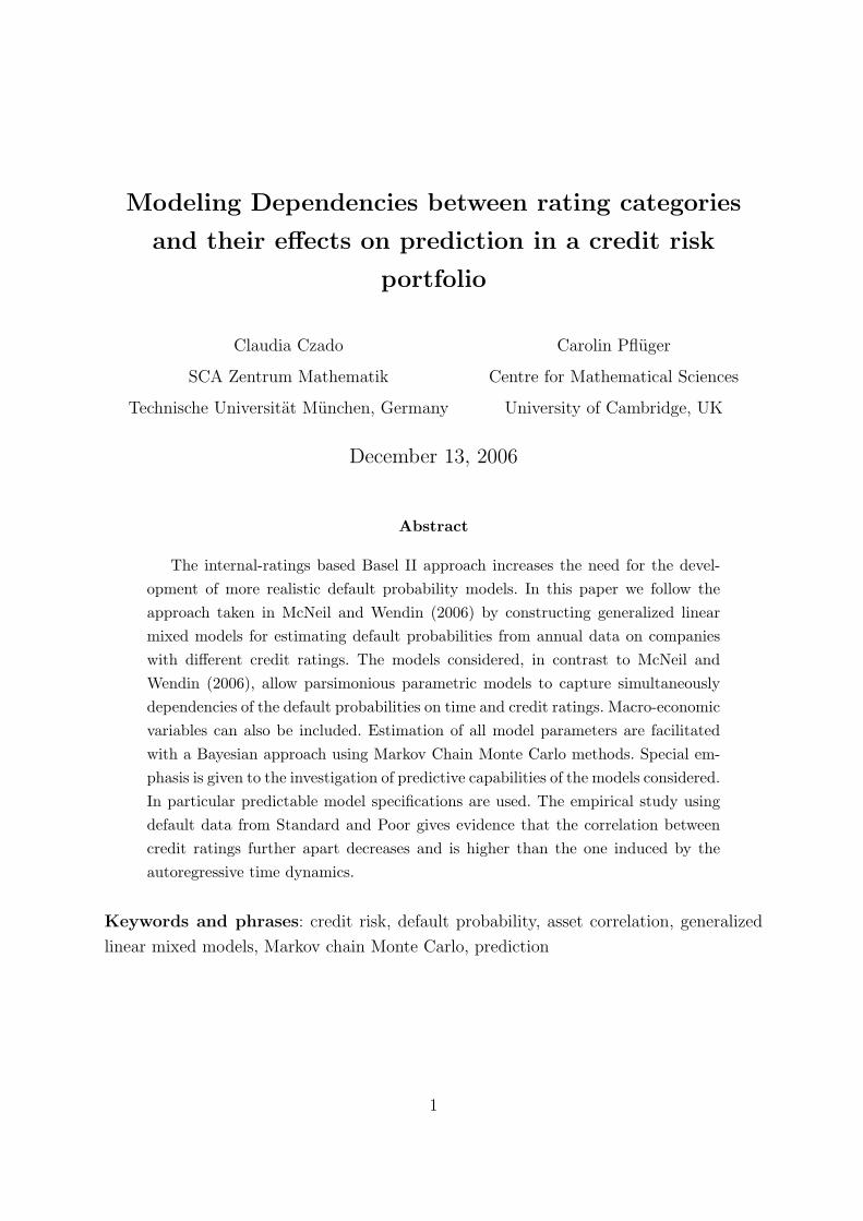
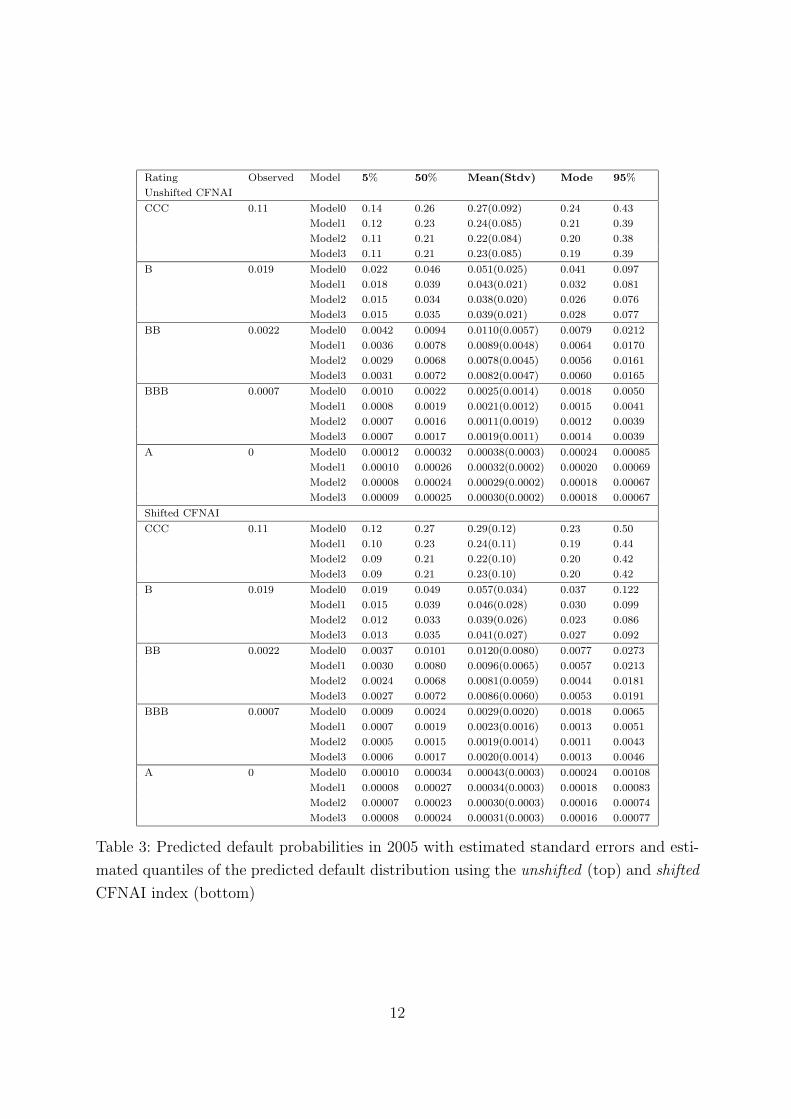
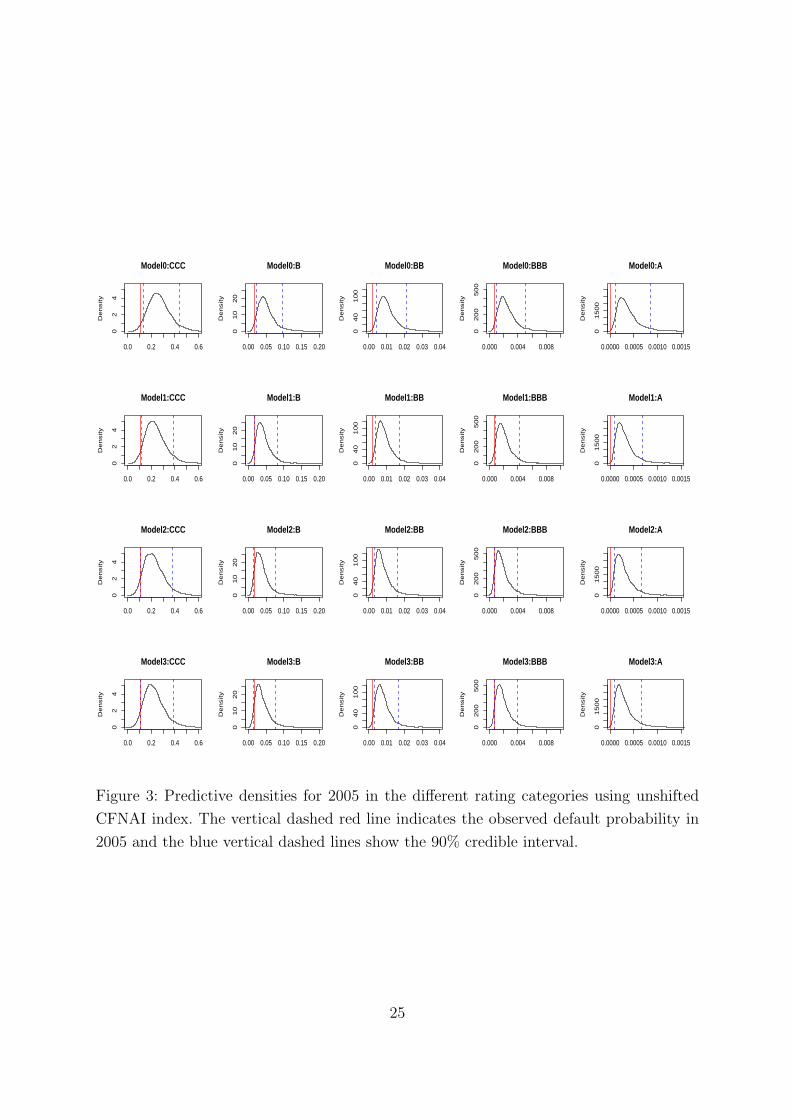
Figure 3 and the top part of Table 3 summarize the predictive distributions for 2005

obtained for the different models using the unshifted CFNAI index. In general the point

predictions such as the mode, mean and median of the predictive distribution are higher

than the observed values. Further, the predictive distributions are skewed with a long

right tail, so that mean and median are to the right of the mode of the distribution.

Comparing the distributions obtained for rating category BBB one can see in Figure 3

that the mode of the distribution is closest to the observed default probability for Model2.

The same effect can be observed in the upper part of Table 3.

[Figure 3 about here]

11

Rating Observed Model 5% 50% Mean(Stdv) Mode 95%

Unshifted CFNAI

CCC 0.11 Model0 0.14 0.26 0.27(0.092) 0.24 0.43

Model1 0.12 0.23 0.24(0.085) 0.21 0.39

Model2 0.11 0.21 0.22(0.084) 0.20 0.38

Model3 0.11 0.21 0.23(0.085) 0.19 0.39

B 0.019 Model0 0.022 0.046 0.051(0.025) 0.041 0.097

Model1 0.018 0.039 0.043(0.021) 0.032 0.081

Model2 0.015 0.034 0.038(0.020) 0.026 0.076

Model3 0.015 0.035 0.039(0.021) 0.028 0.077

BB 0.0022 Model0 0.0042 0.0094 0.0110(0.0057) 0.0079 0.0212

Model1 0.0036 0.0078 0.0089(0.0048) 0.0064 0.0170

Model2 0.0029 0.0068 0.0078(0.0045) 0.0056 0.0161

Model3 0.0031 0.0072 0.0082(0.0047) 0.0060 0.0165

BBB 0.0007 Model0 0.0010 0.0022 0.0025(0.0014) 0.0018 0.0050

Model1 0.0008 0.0019 0.0021(0.0012) 0.0015 0.0041

Model2 0.0007 0.0016 0.0011(0.0019) 0.0012 0.0039

Model3 0.0007 0.0017 0.0019(0.0011) 0.0014 0.0039

A 0 Model0 0.00012 0.00032 0.00038(0.0003) 0.00024 0.00085

Model1 0.00010 0.00026 0.00032(0.0002) 0.00020 0.00069

Model2 0.00008 0.00024 0.00029(0.0002) 0.00018 0.00067

Model3 0.00009 0.00025 0.00030(0.0002) 0.00018 0.00067

Shifted CFNAI

CCC 0.11 Model0 0.12 0.27 0.29(0.12) 0.23 0.50

Model1 0.10 0.23 0.24(0.11) 0.19 0.44

Model2 0.09 0.21 0.22(0.10) 0.20 0.42

Model3 0.09 0.21 0.23(0.10) 0.20 0.42

B 0.019 Model0 0.019 0.049 0.057(0.034) 0.037 0.122

Model1 0.015 0.039 0.046(0.028) 0.030 0.099

Model2 0.012 0.033 0.039(0.026) 0.023 0.086

Model3 0.013 0.035 0.041(0.027) 0.027 0.092

BB 0.0022 Model0 0.0037 0.0101 0.0120(0.0080) 0.0077 0.0273

Model1 0.0030 0.0080 0.0096(0.0065) 0.0057 0.0213

Model2 0.0024 0.0068 0.0081(0.0059) 0.0044 0.0181

Model3 0.0027 0.0072 0.0086(0.0060) 0.0053 0.0191

BBB 0.0007 Model0 0.0009 0.0024 0.0029(0.0020) 0.0018 0.0065

Model1 0.0007 0.0019 0.0023(0.0016) 0.0013 0.0051

Model2 0.0005 0.0015 0.0019(0.0014) 0.0011 0.0043

Model3 0.0006 0.0017 0.0020(0.0014) 0.0013 0.0046

A 0 Model0 0.00010 0.00034 0.00043(0.0003) 0.00024 0.00108

Model1 0.00008 0.00027 0.00034(0.0003) 0.00018 0.00083

Model2 0.00007 0.00023 0.00030(0.0003) 0.00016 0.00074

Model3 0.00008 0.00024 0.00031(0.0003) 0.00016 0.00077

Table 3: Predicted default probabilities in 2005 with estimated standard errors and esti-

mated quantiles of the predicted default distribution using the unshifted (top) and shifted

CFNAI index (bottom)

12

The lower part of Table 3 shows the predicted default probabilities for 2005 but this

time the shifted CFNAI index was used. As one would expect, using this less informative

covariate, one obtains slightly larger standard deviations and larger 90% credible intervals.

However, the modal values are closer to the observed values than in the upper part of

Table 3. This probably is due to the fact that the CFNAI mainly is an indicator for future

economic activity and therefore also is highly relevant for the coming year.

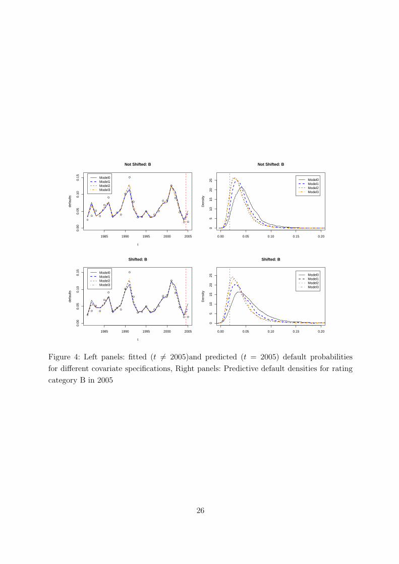
Figure 4 compares fit and prediction obtained for rating category B for all models using

the shifted CFNAI and the unshifted CFNAI. The left panels of Figure 4 give the fitted

(t 6= 2005) and the predicted (t = 2005) default probabilities, while the right panels of

Figure 4 compare the predicted densities for 2005. Clearly the base model Model0 gives

the worst predictions, while the predictions in Model1 are better than Model0 for both the

unshifted and shifted CFNAI specifications. However the predictive distribution of Model2

is the most concentrated predictive distribution with mode closest to the observed value.

[ Figure 4 about here]

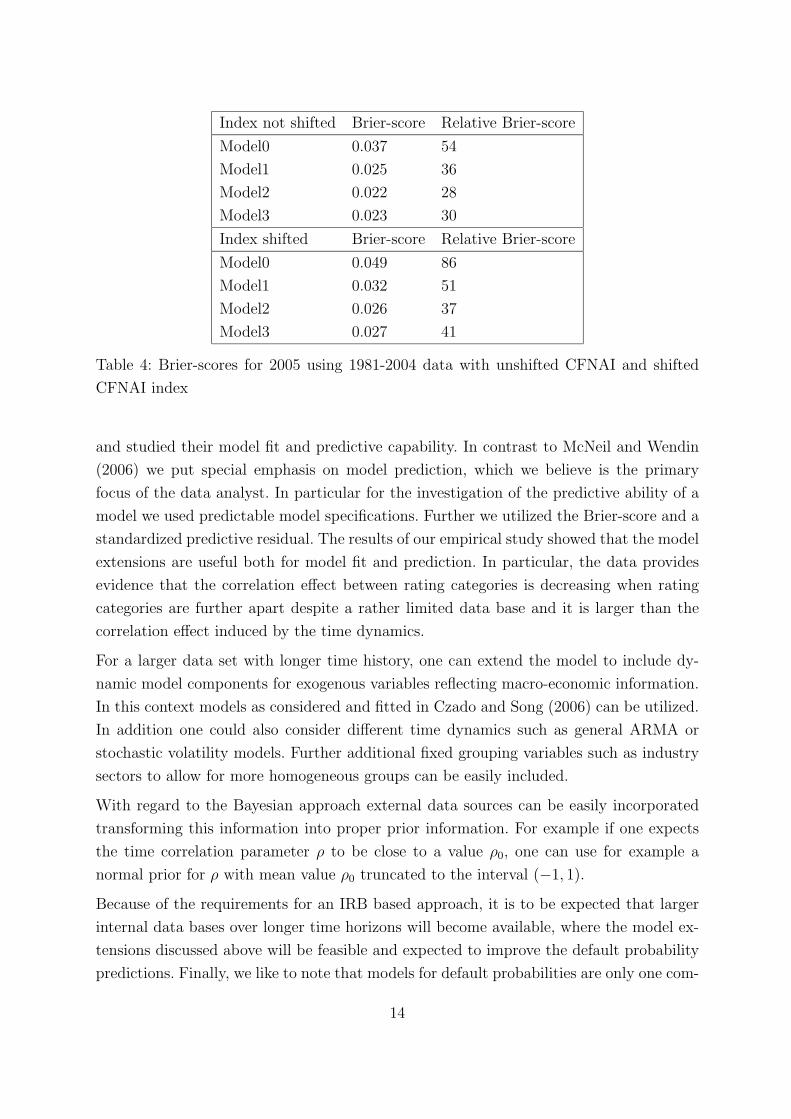
The upper part of Table 4 shows Brier-scores and relative Brier-scores for all models

using the unshifted and the shifted CFNAI index. Since in rating-category A the observed

default probability is 0, we chose to divide by 10−4 instead, which is approximately the

order of magnitude of the predictive default probabilities. Brier-scores using the shifted

CFNAI index are higher for all models but they are still in the range of Brier-scores using

the unshifted CFNAI. That means that while using the shifted CFNAI rather than the

unshifted CFNAI impairs the predictive strength of our models, the predictions obtained

using the shifted CNFAI still are reasonably good. These scores again support that Model2

has the best predictive qualities, closely followed by Model3. The same effects can also

be observed in Table 5. In the top and bottom part Model2 scores best for all rating

categories and for shifted and unshifted CNFAI. Moreover, in the bottom part one can

see that scores using the non-shifted CFNAI are very close to the scores obtained using

the shifted CFNAI. This illustrates again that using the shifted CFNAI does not impair

predictions by much.

Judging from the results on the predictive distributions one would clearly prefer Model2

over Model3.

5 Summary and discussion

We have extended the Bernoulli mixture models considered in McNeil and Wendin (2006)

by explicitly modeling the correlation structure between rating category and time period

13

Index not shifted Brier-score Relative Brier-score

Model0 0.037 54

Model1 0.025 36

Model2 0.022 28

Model3 0.023 30

Index shifted Brier-score Relative Brier-score

Model0 0.049 86

Model1 0.032 51

Model2 0.026 37

Model3 0.027 41

Table 4: Brier-scores for 2005 using 1981-2004 data with unshifted CFNAI and shifted

CFNAI index

and studied their model fit and predictive capability. In contrast to McNeil and Wendin

(2006) we put special emphasis on model prediction, which we believe is the primary

focus of the data analyst. In particular for the investigation of the predictive ability of a

model we used predictable model specifications. Further we utilized the Brier-score and a

standardized predictive residual. The results of our empirical study showed that the model

extensions are useful both for model fit and prediction. In particular, the data provides

evidence that the correlation effect between rating categories is decreasing when rating

categories are further apart despite a rather limited data base and it is larger than the

correlation effect induced by the time dynamics.

For a larger data set with longer time history, one can extend the model to include dy-

namic model components for exogenous variables reflecting macro-economic information.

In this context models as considered and fitted in Czado and Song (2006) can be utilized.

In addition one could also consider different time dynamics such as general ARMA or

stochastic volatility models. Further additional fixed grouping variables such as industry

sectors to allow for more homogeneous groups can be easily included.

With regard to the Bayesian approach external data sources can be easily incorporated

transforming this information into proper prior information. For example if one expects

the time correlation parameter ρ to be close to a value ρ0, one can use for example a

normal prior for ρ with mean value ρ0 truncated to the interval (−1, 1).

Because of the requirements for an IRB based approach, it is to be expected that larger

internal data bases over longer time horizons will become available, where the model ex-

tensions discussed above will be feasible and expected to improve the default probability

predictions. Finally, we like to note that models for default probabilities are only one com-

14

Index not shifted |d2005,CCC | |d2005,B| |d2005,BB| |d2005,BBB| |d2005,A|Model0 3.66 3.96 2.33 1.27 0.63

Model1 3.00 3.15 2.00 1.05 0.58

Model2 2.75 2.57 1.76 0.89 0.55

Model3 2.79 2.69 1.85 0.94 0.56

Index shifted |d2005,CCC | |d2005,B| |d2005,BB| |d2005,BBB| |d2005,A|Model0 4.00 4.36 2.51 1.38 0.67

Model1 3.08 3.25 2.06 1.08 0.59

Model2 2.71 2.47 1.74 0.85 0.55

Model3 2.83 2.72 1.87 0.94 0.57

Index not shifted CPO2005,CCC CPO2005,B CPO2005,BB CPO2005,BBB CPO2005,A

Model0 0.011 0.009 0.032 0.148 0.667

Model1 0.018 0.015 0.049 0.186 0.710

Model2 0.023 0.023 0.071 0.216 0.729

Model3 0.022 0.022 0.063 0.207 0.725

Index shifted CPO2005,CCC CPO2005,B CPO2005,BB CPO2005,BBB CPO2005,A

Model0 0.012 0.010 0.034 0.137 0.640

Model1 0.022 0.018 0.058 0.185 0.698

Model2 0.027 0.025 0.081 0.220 0.730

Model3 0.025 0.023 0.070 0.207 0.719

Table 5: Top Part: Absolute predictive residuals |d2005,k| for k = 1, . . . , K using 1981-2004

data with unshifted CFNAI and shifted CFNAI Bottom Part: Conditional predictive

ordinates CPO2005,k for k = 1, . . . , K using 1981-2004 data with unshifted CFNAI and

shifted CFNAI

15

ponent for credit risk management in addition to models for loss after default. Therefore

more realistic joint models which can be fitted and assessed by a Bayesian approach are

to be envisioned.

References

Bangia, A., F. Diebold, A. Kronimus, C. Schlagen, and T. Schuermann (2002). Rating

migration and the business cycle with application to credit portfolio stress testing.

J. Banking Finance 26, 445–474.

Brier, G. (1950). Verification of forecasts expressed in terms of probability. Monthly

Weather Review 7, 1–3.

Chib, S. (2001). Markov chain Monte Carlo methods: computation and inference. In

Handbook of Econometrics Vol. 5, (Heckman, J. and Leamer, E. (eds)), pp. 3569–

3649. North Holland, Amsterdam.

Czado, C. and P. X. Song (2006). State space mixed models for longitudinal obsser-

vations with binary and binomial responses. Statistical Papers , to appear, preprint

available as Discussion Paper 503 at http://www.stat.uni–muenchen.de/sfb386/.

Demey, P., J. Jouanin, C. Roget, and T. Roncalli (2004). Maximum likelihood estimate

of default correlations. Risk 17-11, 104–108.

Gamerman, D. (1997). Markov Chain Monte Carlo Stoachastic Simulation for Bayesian

Inference (1 ed.). Chapman & Hall, London.

Gelfand, A. (1996). Model determination using sampling-based methods. In Markov

Chain Monte Carlo in Practice (eds Gilks, W. and Richardson, S. and Spiegelhalter,

D., pp. 145–161. London: Chapman & Hall.

Gilks, W. (1992). Derivative-free adaptive rejection sampling for gibbs sampling. In

Bayesian Statistics 4 (eds Bernardo, J.and Berger, J. and Dawid, A. and Smith A.,

pp. 145–161. London: Chapman & Hall.

Gilks, W. (1996). Full conditional distributions. In Markov Chain Monte Carlo in Prac-

tice (eds Gilks, W. and Richardson, S and Spiegelhalter, D., pp. 75–88. London:

Chapman & Hall.

Gilks, W., S. Richardson, and D. Spiegelhalter (1996). Markov Chain Monte Carlo in

Practice (1 ed.). Chapman & Hall, London.

Gordy, M. and E. Heitfield (2002). Estimating default correlations from short panels of

credit performance data. Federal Reserve Board .

16

McNeil, A., R. Frey, and P. Embrechts (2005). Quantitative Risk Management: Con-

cepts, Techniques, and Tools. Princeton University Press.

McNeil, A. and J. Wendin (2006). Bayesian inference for generalized linear mixed mod-

els of portfolio credit risk. Journal of Emprical Finance, to appear.

Merton, R. (1974). On the pricing of corporate debt: The risk structure of interest rates.

J. Finance 29, 449–470.

Nickell, P., W. Perraudin, and S. Varotto (2000). Stability of rating transitions. J.

Banking Finance 24, 203–227.

Servigny, A. and O. Renault (2003). Correlation evidence. Risk July 2003, 90–94.

Spiegelhalter, D. J., N. G. Best, B. P. Carlin, and A. van der Linde (2002). Bayesian

measures of model complexity and fit. Journal of the Royal Statistical Society B 64,

583–639.

17

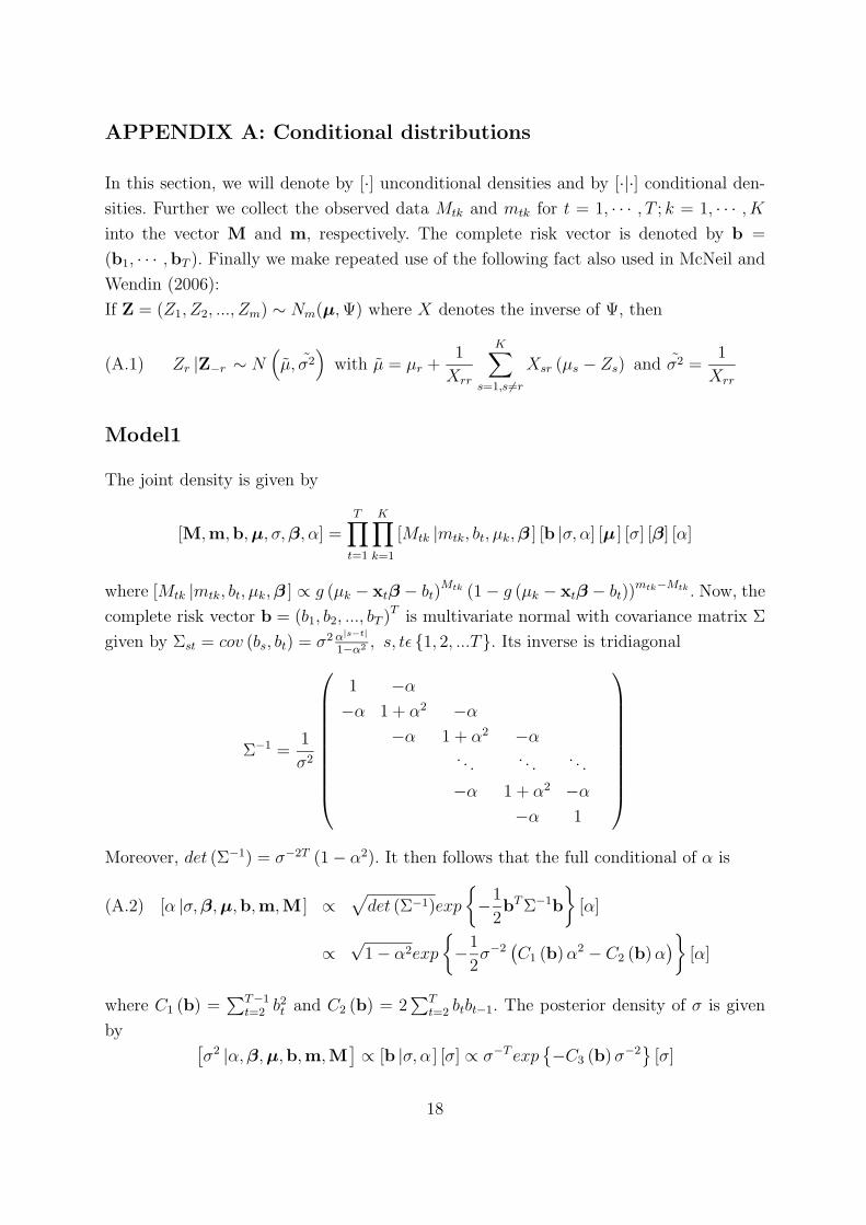
APPENDIX A: Conditional distributions

In this section, we will denote by [·] unconditional densities and by [·|·] conditional den-

sities. Further we collect the observed data Mtk and mtk for t = 1, · · · , T ; k = 1, · · · , K

into the vector M and m, respectively. The complete risk vector is denoted by b =

(b1, · · · ,bT ). Finally we make repeated use of the following fact also used in McNeil and

Wendin (2006):

If Z = (Z1, Z2, ..., Zm) ∼ Nm(µ, Ψ) where X denotes the inverse of Ψ, then

(A.1) Zr |Z−r ∼ N(

µ, σ2)

with µ = µr +1

Xrr

K∑

s=1,s 6=r

Xsr (µs − Zs) and σ2 =1

Xrr

Model1

The joint density is given by

[M,m,b,µ, σ,β, α] =T

∏

t=1

K∏

k=1

[Mtk |mtk, bt, µk,β ] [b |σ, α] [µ ] [σ] [β] [α]

where [Mtk |mtk, bt, µk,β ] ∝ g (µk − xtβ − bt)Mtk (1 − g (µk − xtβ − bt))

mtk−Mtk . Now, the

complete risk vector b = (b1, b2, ..., bT )T is multivariate normal with covariance matrix Σ

given by Σst = cov (bs, bt) = σ2 α|s−t|

1−α2 , s, tǫ {1, 2, ...T}. Its inverse is tridiagonal

Σ−1 =1

σ2

1 −α

−α 1 + α2 −α

−α 1 + α2 −α. . . . . . . . .

−α 1 + α2 −α

−α 1

Moreover, det (Σ−1) = σ−2T (1 − α2). It then follows that the full conditional of α is

[α |σ,β,µ,b,m,M ] ∝√

det (Σ−1)exp

{

−1

2bT Σ−1b

}

[α](A.2)

∝√

1 − α2exp

{

−1

2σ−2

(

C1 (b) α2 − C2 (b) α)

}

[α]

where C1 (b) =∑T−1

t=2 b2t and C2 (b) = 2

∑T

t=2 btbt−1. The posterior density of σ is given

by[

σ2 |α,β,µ,b,m,M]

∝ [b |σ, α ] [σ] ∝ σ−T exp{

−C3 (b) σ−2}

[σ]

18

where C3 (b) = 12

(

∑T

t=1 b2t + α2

∑T−1t=2 b2

1 − 2α∑T

t=2 btbt−1

)

. But now, if σ2 has an

InvΓ (η, ν) prior then

[

σ2 |α,β,µ,b,m,M]

∼ InvΓ (η + T/2, ν + C3 (b, α)) .

The risk vector b |α, σ is multivariate normal and for b−t = (b1, b2, ..., bt−1, bt+1, ..., bT ),

t = 1, 2, . . . T

[

bt

∣

∣b−t, α, σ]

∼

N (αb2, σ2) t = 1

N (αbT−1, σ2) t = T

N(

α1+α2 (bt−1 + bt+1) , σ2

1+α2

)

) otherwise

The full conditional density then is

[bt |b−t, α, σ,m,M ] ∝K∏

k=1

[Mtk |mtk, bt, µk ] [bt |b−t, α, σ ]

where [Mtk |mtk, bt, µk,β ] ∝ g (µk − xtβ − bt)Mtk (1 − g (µk − xtβ − bt))

mtk−Mtk . The full

conditional density of β is given by

[β |α, σ,µ,b,m,M ] ∝T

∏

t=1

K∏

k=1

[Mtk |mtk, bt, µk,β] [β ] .

The corresponding full conditionals for Model0 can easily be obtained by setting α = 0.

Model2

Model2 has the joint distribution

(A.3) [M,m,b,µ, σ, α,β, ρ] =T

∏

t=1

K∏

k=1

[Mtk |mtk, btk, µk, β ] [b |σ, αρ ] [µ] [σ] [α] [β] [ρ] ,

The risk vector b is again multivariate normal with zero mean vector and cov (bsk, btl) =

Φklα|t−s|

1−α2 , s, tǫ {1, 2, . . . , T}, k, lǫ {1, 2, . . . , K} so that the covariance matrix has inverse

(A.4) Σ−1 =1

σ2

Λ −αΛ

−αΛ Λ (1 + α2) −αΛ

−αΛ Λ (1 + α2) −αΛ.. . . . . . . .

−αΛ Λ (1 + α2) −αΛ

−αΛ Λ

19

where

Λ =

1 −ρ

−ρ 1 + ρ2 −ρ

−ρ 1 + ρ2 −ρ. . . . . . . . .

−ρ 1 + ρ2 −ρ

−ρ 1

is the inverse of Φ/σ2. This gives that det (Σ−1) = det (Λ)T (1 − α2) σ−2TK =

σ−2TK (1 − ρ2)T

(1 − α2). Now, b is again multivariate normal and it follows from (A.1)

that

(A.5) [bt |b−t, α,β, σ, ρ ] ∼

N (αb2, Φ) t = 1

N (αbT−1, Φ) t = T

N(

α1+α2 (bt−1 + bt+1) , 1

1+α2 Φ)

) otherwise

Again using A.1 gives that if t = 1

[btk |b−tk, α,β, ρ, σ ] ∼

N(

αb2,k − ρ (αb2,k+1 − b1,k+1) , σ2)

k = 1

N(

αb2,k − ρ (αb2,k−1 − b1,k−1) , σ2)

k = K

N(

αb2,k − ρ1+ρ2 (αb2,k−1 − b1,k−1 + αb2,k+1 − b1,k+1) , σ2

1+ρ2

)

otherwise

If t = T

[btk |b−tk, α,β, ρ, σ ] ∼

N(

αbT−1,k − ρ (αbT−1,k+1 − bT,k+1) , σ2)

k = 1

N(

αbT−1,k − ρ (αbT−1,k−1 − bT,k−1) , σ2)

k = K

N(

αbT−1,k − ρ1+ρ2 (αbT−1,k−1 − bT,k−1+

αbT−1,k+1 − bT,k+1) , σ2

1+ρ2

)

otherwise

For 1 < t < T

[btk |b−tk, α,β, ρ, σ ] ∼

N(

α1+α2 (bt−1,k + bt+1,k) − ρ

(

α1+α2 (bt−1,k+1 + bt+1,k+1) − bt,k+1

)

, σ2

1+α2

)

k = 1

N(

α1+α2 (bt−1,k + bt+1,k) − ρ

(

α1+α2 (bt−1,k−1 + bt+1,k−1) − bt,k−1

)

, σ2

1+α2

)

k = K

N

(

α

1 + α2(bt−1,k + bt+1,k) −

ρ

1 + ρ2

[

α

1 + α2(bt−1,k−1 + bt+1,k−1)

−bt,k−1 + α1+α2 (bt−1,k+1 + bt+1,k+1) − bt,k+1)

]

, σ2

(1+ρ2)(1+α2)

)

otherwise

Then [btk |b−tk, α,β, ρ, σ,m,M ] ∝ [btk |b−tk, α, ρ, σ, ] [Ntk |ntk, btk, µk,β ]. The full condi-

20

tional distribution of ρ is given by

[ρ |α, σ,β,m,M,b ] ∝ [b |σ, ρ, α ] [ρ]

∝√

det (Σ−1)exp

{

−1

2bT Σ−1b

}

[σ]

∝√

(1 − ρ2)T exp

{

−1

2σ−2

(

S1 (b, α) ρ + S2 (b, α) ρ2)

}

Now, if ci (u,v) denotes the coefficient of ρi in uT Λv, then here c1 (u,v) =

−(

∑K

k=2 ukvk−1 + uk−1vk

)

and c2 (u,v) =∑K−1

k=2 ukvk. Then for i = 1, 2

(A.6) Si (b, α) =T−1∑

t=2

(

ci (bt,bt)(

1 + α2))

+ ci (b1,b1) + ci (bT ,bT ) − 2αT

∑

t=2

ci (bt,bt)

The full conditional distribution of α can be determined as in A.2

[α |σ,β, ρ,µ,b,m,M ] ∝√

det (Σ−1)exp

{

−1

2bT Σ−1b

}

[α]

∝√

1 − α2exp

{

−1

2σ−2

(

C1 (b, Λ) α2 − C2 (b, Λ) α)

}

[α]

where C1 (b, Λ) =∑T−1

t=2 btT Λbt and C2 (b) =

∑T

t=2 btT Λbt−1 +bt−1

T Λbt. The posterior

density of σ2 is given by

[

σ2 |α,β, ρ,µ,b,m,M]

∝ [b |σ, ρ, α ] [σ] ∝√

det (Σ)−1exp

{

−1

2bT Σ−1b

}

[σ]

∝ σ−TKexp{

−C3 (b, Λ, α) σ−2}

[σ]

where C3 (b, Λ, α) = 12

(

∑T

t=1 btT Λbt + α2

∑T−1t=2 bt

T Λbt − α∑T

t=2

(

btT Λbt−1 + bt−1

T Λbt

)

)

.

Then, if σ2 has an InvΓ (η, ν) prior

[

σ2 |α,β, ρ,µ,b,m,M]

∼ InvΓ (η + TK/2, ν + C3 (b, Λ, α))

The posterior densities for β and µ can be found similarly to those in Model1.

Model3

Model3 again has joint density (A.3). Here, the covariance matrix has inverse as in (A.4)

where Λ is the inverse of Φ1−ρ2

σ2 with Φ defined in (2.6) i.e

(A.7) Λ =1 + 3ρ

1 + 3ρ − 4ρ2

1 λ λ λ λ

λ 1 λ λ λ

λ λ 1 λ λ

λ λ λ 1 λ

λ λ λ λ 1

with λ =−ρ

1 + 3ρ.

21

This then gives

det(

Σ−1)

= det (Λ)T(

1 − α2)

σ−2TK =

(

(1 − λ)4 (1 + 4λ)

(

1 + 3ρ

1 + 3ρ − 4ρ2

)K)T

σ−2TK(

1 − α2)

.

(A.5) and (A.1) hold exactly as for Model2 and with Λ as above [btk |b−tk, α,β, ρ, σ ] can

be determined. For t = 1

[btk |b−tk, α,β, ρ, σ ] ∼ N

(

αb2,k + λ∑

s 6=k

(αb2,s − b1,s) ,1 + 3ρ − 4ρ2

1 + 3ρσ2

)

.

For t = T

[btk |b−tk, α,β, ρ, σ ] ∼ N

(

αbT−1,k + λ∑

s 6=k

(αbT−1,s − bT,s) ,1 + 3ρ − 4ρ2

1 + 3ρσ2

)

.

For 1 < t < T

[btk |b−tk, α,β, ρ, σ ] ∼ N

(

α

1 + α2(bt−1,k + bt+1,k)

+λ∑

s 6=k

(

α

1 + α2(bt−1,s + bt+1,s) − bt,s

)

, σ2 1

1 + α2

1 + 3ρ − 4ρ2

1 + 3ρ

)

The full conditional density of ρ is determined by

[ρ |α, σ, β,m,M,b ] ∝ [b |σ, ρ, α ] [ρ] ∝√

det (Σ−1)exp

{

−1

2bT Σ−1b

}

[σ]

∝

(

1

1 + 4ρ

1

(1 − ρ)4

) T

2

exp

{

−1

2ρ2

(

1 + 3ρ

1 + 3ρ − 4ρ2S1 (b, α) − S2 (b, α)

ρ

1 + 3ρ − 4ρ2

)}

Now, if ci (u,v) this time denotes the coefficient of λi in uT 1+3ρ−4ρ2

1+3ρΛv for Λ defined in

(A.7) then here c1 (u,v) =∑

k ukvk and c2 (u,v) =∑

k 6=l ukvl. Then for i = 1, 2 Si is

again defined by (A.6). Since the full conditional distributions of α, β, σ and µ do not

depend on the actual form of Λ these full conditional distributions are the same as in

Model2.

22

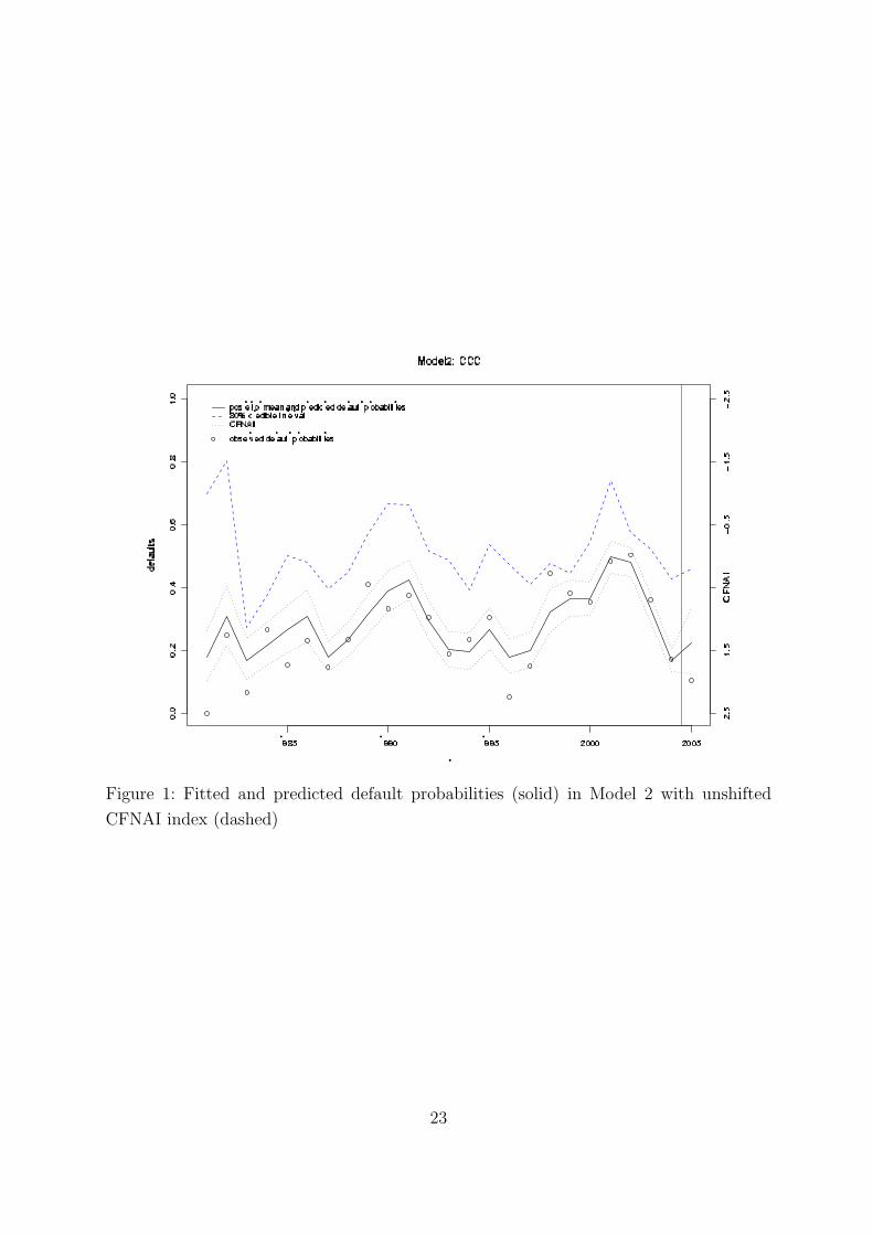
Figure 1: Fitted and predicted default probabilities (solid) in Model 2 with unshifted

CFNAI index (dashed)

23

1985 1990 1995 2000 2005

0.0

0.2

0.4

0.6

de

fau

lts

Model0: CCC

1985 1990 1995 2000 2005

0.0

0.2

0.4

0.6

de

fau

lts

Model1: CCC

1985 1990 1995 2000 2005

0.0

0.2

0.4

0.6

de

fau

lts

Model2: CCC

1985 1990 1995 2000 2005

0.0

0.2

0.4

0.6

de

fau

lts

Model3: CCC

1985 1990 1995 2000 2005

0.0

00

.10

de

fau

lts

Model0: B

1985 1990 1995 2000 2005

0.0

00

.10

de

fau

lts

Model1: B

1985 1990 1995 2000 2005

0.0

00

.10

de

fau

lts

Model2: B

1985 1990 1995 2000 2005

0.0

00

.10

de

fau

lts

Model3: B

1985 1990 1995 2000 2005

0.0

00

.02

0.0

4

de

fau

lts

Model0: BB

1985 1990 1995 2000 2005

0.0

00

.02

0.0

4

de

fau

lts

Model1: BB

1985 1990 1995 2000 2005

0.0

00

.02

0.0

4

de

fau

lts

Model2: BB

1985 1990 1995 2000 2005

0.0

00

.02

0.0

4

de

fau

lts

Model3: BB

1985 1990 1995 2000 2005

0.0

00

0.0

06

0.0

12

de

fau

lts

Model0: BBB

1985 1990 1995 2000 2005

0.0

00

0.0

06

0.0

12

de

fau

lts

Model1: BBB

1985 1990 1995 2000 2005

0.0

00

0.0

06

0.0

12

de

fau

lts

Model2: BBB

1985 1990 1995 2000 2005

0.0

00

0.0

06

0.0

12

de

fau

lts

Model3: BBB

Figure 2: Estimated posterior mean default probabilities for t = 1981, . . . , 2004 and pre-

dicted default probability for 2005 (solid line) with 80% credible intervals (dotted lines)

and observed default probabilities (o) using the unshifted CFNAI index.

24

0.0 0.2 0.4 0.6

02

4

Model0:CCC

De

nsity

0.0 0.2 0.4 0.6

02

4

Model1:CCC

De

nsity

0.0 0.2 0.4 0.6

02

4

Model2:CCC

De

nsity

0.0 0.2 0.4 0.6

02

4

Model3:CCC

De

nsity

0.00 0.05 0.10 0.15 0.20

01

02

0

Model0:B

De

nsity

0.00 0.05 0.10 0.15 0.20

01

02

0

Model1:B

De

nsity

0.00 0.05 0.10 0.15 0.20

01

02

0

Model2:B

De

nsity

0.00 0.05 0.10 0.15 0.20

01

02

0

Model3:B

De

nsity

0.00 0.01 0.02 0.03 0.040

40

10

0

Model0:BB

De

nsity

0.00 0.01 0.02 0.03 0.04

04

01

00

Model1:BB

De

nsity

0.00 0.01 0.02 0.03 0.04

04

01

00

Model2:BB

De

nsity

0.00 0.01 0.02 0.03 0.04

04

01

00

Model3:BB

De

nsity

0.000 0.004 0.008

02

00

50

0

Model0:BBB

De

nsity

0.000 0.004 0.0080

20

05

00

Model1:BBB

De

nsity

0.000 0.004 0.008

02

00

50

0

Model2:BBB

De

nsity

0.000 0.004 0.008

02

00

50

0

Model3:BBB

De

nsity

0.0000 0.0005 0.0010 0.0015

01

50

0

Model0:A

De

nsity

0.0000 0.0005 0.0010 0.0015

01

50

0

Model1:A

De

nsity

0.0000 0.0005 0.0010 0.0015

01

50

0

Model2:A

De

nsity

0.0000 0.0005 0.0010 0.0015

01

50

0

Model3:A

De

nsity

Figure 3: Predictive densities for 2005 in the different rating categories using unshifted

CFNAI index. The vertical dashed red line indicates the observed default probability in

2005 and the blue vertical dashed lines show the 90% credible interval.

25

1985 1990 1995 2000 2005

0.00

0.05

0.10

0.15

t

defa

ults

Not Shifted: B

Model0Model1Model2Model3

1985 1990 1995 2000 2005

0.00

0.05

0.10

0.15

t

defa

ults

Shifted: B

Model0Model1Model2Model3

0.00 0.05 0.10 0.15 0.20

05

1015

2025

Not Shifted: B

Den

sity

Model0Model1Model2Model3

0.00 0.05 0.10 0.15 0.20

05

1015

2025

Shifted: B

Den

sity

Model0Model1Model2Model3

Figure 4: Left panels: fitted (t 6= 2005)and predicted (t = 2005) default probabilities

for different covariate specifications, Right panels: Predictive default densities for rating

category B in 2005

26