MODELING, DESIGN, AND CONTROL OF

MODELING, DESIGN, AND CONTROL OF FORCED-FEEDBACK METERING POPPET VALVE SYSTEM

A Thesis presented to the faculty of the Graduate School University of Missouri-Columbia

In Partial Fulfillment Of the Requirements for the Degree

Master of Science

by

MATTHEW MULLER

Dr. Roger Fales, Thesis Supervisor

May 2006

The undersigned, appointed by the dean of the Graduate School, have examined the project entitled

MODELING, DESIGN, AND CONTROL OF FORCED-FEEDBACK METERING POPPET VALVE SYSTEM

Presented by MATTHEW MULLER a candidate for the degree of Masters of Science and hereby certify that in their opinion it is worthy of acceptance ------------------------------------------------------------------------------------------------------------ Dr. Roger C. Fales, Assistant Professor, Mechanical and Aerospace Engineering ------------------------------------------------------------------------------------------------------------Dr. Noah Manring, J.C. Dowell Prof (MAE), Associate Dean of Research (CoE) ------------------------------------------------------------------------------------------------------------ Dr. Steven C. Borgelt, Associate Professor, Biological Engineering

ACKNOWLEDGMENTS

The opportunity to attend graduate school at the University of Missouri has

been a blessing that I have found continually challenging and rewarding. I am

forever grateful to all the teachers and friends whom have constantly dealt with

my endless questions.

I am especially thankful to my academic advisor, Dr. Roger Fales for his

constant patience and willingness to teach me the many aspects of hydraulics

and controls theory. If it were not for his support, I would not know what a

metering poppet valve was, let alone be able to deal with the many obstacles this

research presented.

I am also thankful to Dr. Manring for his open door to my questions

regarding hydraulics and his accepting to serve on my thesis committee. His

knowledge and his book have provided a constant resource for this project.

I express my appreciation to Dr. Borgelt for generously giving up his time

to examine my thesis and serve on my masters committee.

I will forever be grateful to my parents whom have always encouraged the

quest for knowledge and whose example provides endless motivation.

Last and most profoundly, I owe this entire experience to my wife JoAnn

who not only listened to my daily challenges but made it possible for me to return

to graduate school.

ii

TABLE OF CONTENTS

Acknowledgements………………………………………………………………..……ii

List of Figures………………………………………………………………………...…vi

Abstract…………………………………………………………………………………..xi

Chapter 1. Introduction……………………………………………………………….1

1.1 Motivation and Literature Review………………………………………....1

1.2 Research Objectives……………………………………………………….2

1.3 Forced Feedback Principles……………………………………………….3

1.4 Thesis Outline……………………………………………………………….6

Chapter 2. Mathematical Modeling of the Constant Orifice Approach………8

2.1 Nonlinear Constant Orifice Model…………………………………………8

2.2 Model Linearization…………………………………………….…………10

Chapter 3. Iterative Root Locus Analysis and Design…………………………13

3.1 Iterative Design Procedure……………………………………………….13

3.2 Root Locus Plots for the Constant Orifice Model………………………14

Chapter 4. Variable Orifice Vs. Constant Orifice Models……………….…….22

4.1 Equations for the Variable Orifice Model……………………………….22

4.2 Criteria for Constant Verses Variable Orifice Model Comparisons…..22

4.3 Simulation Comparisons………………………………………………….25

4.4 Design Information Obtained from Model Comparisons………………28

Chapter 5. Examination of Previously Unmodeled Dynamics……………….32

5.1 An 8-State Model………………………………………………………….32

iii

5.2 Validation of 8-State Model Linearization………………………………34

5.3 8-State vs. 5-State Model………………………………………………37

Chapter 6. Mechanical and Electronic Control Designs………………………41

6.1 Introduction to Flow Control……………………………………...………41

6.2 Mechanical Pressure Compensation for Flow Control………………..42

6.3 Electronic Flow Control…………………………………………………...44

6.3.1 Table Look-up Control………………………………………….44

6.3.2 Table Look-up with PD Control……………………………….48

6.3.3 Gain Scheduled PD Control…………………………………..51

6.3.4 Table Look-up with Gain Scheduled PD Control…………...54

6.4 Flow Control Summary……………………………………………………56

6.5 Observer Design…………………………………………………………..57

Chapter 7. Robust Control Analysis………………………………………………64

7.1 Introduction to Robust Analysis………………………………………….64

7.2 Nominal Performance and the Sensitivity Transfer Function………..65

7.3 Derivation of Robust Stability with Multiplicative Uncertainty………...67

7.4 Multiplicative Uncertainty Weighting Function WI……………………...69

7.5 Robust Stability and Performance Results……………………………..71

Chapter 8. Conclusions……………………………………………………………..73

8.1 Overview……………………………………………………………………73

8.2 Research limitations………………………………………………………75

8.3 Scope for future work……………………………………………………..75

iv

Appendix……………………………………………………………………………..…77

References…………………………………………………………………………..…80

v

LIST OF FIGURES

Fig. 1.1 Forced feedback poppet configuration .................................................... 4

Fig. 1.2 Forced feedback poppet with a constant inlet orifice to control volume... 6

vi

sFig. 3.1 Root locus varying ( 21a 1 , 2.1 )P MPa P MPaΔ ≈ 5f N= .............................. 15 =

Fig. 3.2 Zoom of the right portion of Fig. 3.1....................................................... 15

Fig. 3.3 Root locus varying 3h ( 21 , 2.1 )sP MPa P MPaΔ ≈ 5f N= ............................ 16 =

Fig. 3.4 Root locus varying 2h ( 21 , 2.1 )sP MPa P MPaΔ ≈ 5f N= ............................ 16 =

Fig. 3.5 Root locus varying (spring rate) k ( 21 , 2.1 )sP MPa P MPaΔ ≈ 5f N= ......... 17 =

Fig. 3.6 Root locus varying xb (pilot damping) ( 21 , 2.1 )sP MPa P MPaΔ ≈ 5f N= .... 17 =

Fig. 3.7 Root locus varying k ( 21 , 2.1 )sP MPa P MPaΔ ≈ 30f N= ........................... 19 =

Fig. 3.8 Root locus varying a1 ( 35 35 )sP MPa P MPaΔ ≈ 5f N= ............................. 19 =

Fig. 3.9 Root locus varying k ( 35 35 )sP MPa P MPaΔ ≈ 5f N= .............................. 20 =

Fig. 3.10 Root locus varying 4kc ( 21 , 2.1 )sP MPa P MPaΔ ≈ 5f N= .......................... 20 =

Fig. 4.1 Control volume inlet and outlet orifices .................................................. 23

Fig. 4.2 Roots for linearization with 2.1 MPa pressure drop and valve open 0.2

mm ................................................................................................................ 24

Fig. 4.3 Zoom in for the roots on the right side of Fig. 4.2 .................................. 24

Fig. 4.4 Frequency response for both models ( 21 , 1s )P MPa P MPa= Δ = ................... 25

Fig. 4.5 Main poppet position in response to step input force from 0-.2 s, F=50.2

vii

)N for variable orifice, F= 51.4 for constant orifice ( 2.1 , 1sP MPa P MPa= Δ = ........ 26

Fig. 4.6 Main poppet position in response to step input force, F=48.8 N for

variable orifice, F= 54.6 for constant orifice ( 35 , 35s )P MPa P MPa= Δ ≈ ............... 26

Fig. 4.7 Flow out of the control volume for main poppet response of Fig. 4.6

( 35 , 35s )P MPa P MPa= Δ ≈ ................................................................................... 27

Fig. 4.8 Main poppet cracked open in response to step input force, F=8.1 N for

variable orifice, F=13.6 N for constant orifice ( 35 , 35sP MPa P MPa)= Δ ≈ ............ 28

Fig. 4.9 Main poppet response to a solenoid input force from 0-.2 s. Constant

orifice model modified for stability as compared to Fig.

4.5 ................................................................................ 29 ( 2.1 , 1sP MPa P MPa= Δ = )

)

Fig. 4.10 Main poppet response to solenoid input force. Constant orifice model

modified for stability as compared to Fig. 4.6 ( 35 , 35sP MPa P MPa= Δ ≈ ............ 30

Fig. 4.11 Frequency response for both versions of the constant orifice model

( 21 , 1s )P MPa P MPa= Δ = ..................................................................................... 31

Fig. 5.1 Main poppet position for a unit step input .............................................. 35

Fig. 5.2 Main poppet velocity for a unit step input............................................... 35

Fig. 5.3 Pilot poppet position for a unit step input ............................................... 35

Fig. 5.4 Pilot poppet velocity for a unit step input ............................................... 36

Fig. 5.5 Control volume pressure for a unit step input ........................................ 36

Fig. 5.6 Pilot control volume pressure for a unit step input ................................. 36

Fig. 5.7 Load volume pressure for a unit step input............................................ 37

Fig. 5.8 Load piston velocity for a unit step input................................................ 37

viii

)Fig. 5.9 Roots for linearization with valve open 0.2 mm ( 21 , 2.1sP MPa P MPa= Δ ≈ . 38

Fig. 5.10 Zoom in for the right side of Fig. 5.9 .................................................... 38


( 21 , 1s )P MPa P MPa= Δ = ..................................................................................... 40

Fig. 6.1 System with compensator, metering poppet valve, and load................. 42

Fig. 6.2 Valve flow for pressure compensated models (desired flow 30LPM) ... 43

Fig. 6.3 Pressure drop from supply to load pressure .......................................... 43

Fig. 6.4 Poppet valve control scheme with look-up table.................................... 44

Fig. 6.5 Look-up table control vs pressure compensation, desired flow 30 LPM,

see Fig. 6.3 for pressure drop ....................................................................... 45

Fig. 6.6 Look-up table control vs pressure compensation, desired flow 110 LPM,


Fig. 6.7 Varying desired flow between 10 and 100 LPM, pressure drop approx

30MPa........................................................................................................... 47

Fig. 6.8 Varying desired flow between 10 and 70 LPM, pressure drop approx 1

MPa............................................................................................................... 47

Fig. 6.9 Electronic control with look-up table and PD control.............................. 48

Fig. 6.10 Look-up table control vs look-up plus PD control, desired flow 110 LPM,



30MPa........................................................................................................... 50


MPa............................................................................................................... 50

Fig. 6.13 Root locus for negative feedback of flow (35 Mpa pressure drop)....... 52

Fig. 6.14 Root locus for negative feedback of flow (1 Mpa pressure drop)......... 52

Fig. 6.15 Gained scheduled PD controller based on measured pressure drop .. 53

Fig. 6.16 Look-up table control vs gain scheduled PD control, desired flow 110

LPM, see Fig. 6.3 for pressure drop.............................................................. 53


30 MPa.......................................................................................................... 54


MPa............................................................................................................... 54

Fig. 6.19 Gain scheduled Pd control with look-up table...................................... 55

Fig. 6.20 Look-up table control vs look-up table with gained PD control, desired

flow 110 LPM, see Fig. 6.3 for pressure drop................................................ 55


30MPa........................................................................................................... 56


MPa............................................................................................................... 56

Fig. 6.23 Observer estimate of main poppet position ......................................... 59

Fig. 6.24 Observer estimate of main poppet velocity.......................................... 60

Fig. 6.25 Observer estimate of pilot poppet position........................................... 60

ix

Fig. 6.26 Observer estimate of pilot poppet velocity ........................................... 60

Fig. 6.27 Observer estimate of pressure above main poppet ............................. 61

Fig. 6.28 Observer estimate of pressure above pilot poppet .............................. 61

Fig. 6.29 Observer estimate of load pressure (measured) ................................. 61

Fig. 6.30 Observer estimate of load piston velocity ............................................ 62

Fig. 6.31 Observer flow estimate vs. ‘true’ flow .................................................. 63

Fig. 7.1 PD/table look-up control with pressure drop held constant.................... 66

Fig. 7.2 Block diagram reduction for calculating sensitivity transfer function ...... 66

Fig. 7.3 Nominal Performance for 3 pressure drops when the valve is cracked

open .............................................................................................................. 67

Fig. 7.4 Control scheme with multiplicative uncertainty included........................ 68

Fig. 7.5 configuration for determining RS criteria ......................................... 68 NΔ

Fig. 7.6 Block diagram for determining robust stability criterion.......................... 69

Fig. 7.7 for worst case plant at 1 MPa pressure drop .................................... 71 IW

Fig. 7.8 Robust stability for 3 pressure drops with the valve cracked open ........ 72

Fig. 7.9 Robust performance for 3 pressure drops with the valve cracked open 72

x

ABSTRACT

This research explores valve design, dynamic modeling, and techniques

to achieve flow control for a forced-feedback metering poppet valve system. In

particular, nonlinear and linear models of a forced feedback configuration are

developed and tuned through the use of root locus techniques. Typical steady

state conditions as well as extreme high and low pressure drops are simulated in

attempts to uncover instabilities and other possible undesirable performance

characteristics of the valve. It is shown that by using a variable inlet orifice to the

control volume as opposed to a constant orifice, desired system bandwidth and

stability can be achieved. Open loop valve designs are then simulated with

several electronic control schemes which incorporate feedback of load pressure

and in some cases valve flow. An observer design is investigated as a means of

providing flow feedback without additional sensor costs. Electronic flow control

schemes are compared to standard mechanical pressure compensation and

finally a robust analysis is provided for a chosen electronic control scheme.

xi

CHAPTER 1

INTRODUCTION

1.1 Motivation and Literature Review:

Electro-hydraulic control valves are extensively used in industry to control

motion in various devices. For many years the standard has been to use spool

type valves along with separate supply pressures for the pilot and main stages of

flow control valves. Poppet valves have been available for many years but have

been limited in use to situations such as pressure relief. Over the past ten years

there has been a push to develop poppet valves that can meter flow in the way

spool valves have typically been used [1,2,3,4,5]. The incentives behind this

growing trend are the advantages that come with the use of poppet valves. In

comparison to spool valves, poppet valves require less stringent machining

tolerances, are less susceptible to contamination problems, have very low

leakage, and make it possible to eliminate two separate supply lines [6,7].

Although poppet valves present many advantages to spool valves they have yet

to take over the market due to a long history of instability issues. The instabilities

in poppet valve circuits have been studied by Hayashi [8] , Funk [9], Wandling

[10], and others but there is still no clear path to avoiding this problem. Hayashi

1

[8] suggests it is important to examine valve motions with small valve lift and

hysteresis of flow forces. Funk [9] presents claims that instability can be caused

by interaction between the poppet spring-mass system and line dynamics.

McCloy [11] examines the effects steady-state flow forces in various valve

systems while more recently Johnston et al. [12] provides experimental

investigations into poppet flow forces. In recent years there have been metering

poppet valves that have proved successful enough to become commercially

available. Zhang et al. [1] studies the dynamics of one such valve and suggest

performance limitations due to zero location. Fales [13] studies the performance

and stability of the same valve as Zang [1] and demonstrates the importance of

pressure drop in the analysis. Opdenbosch et al. [14] models a newer poppet

valve with a position follower configuration and proposes a controller based on a

Nodal Link Perceptron Network. The list of papers in the open literature in

regards to modeling the dynamics of metering poppet valves surrounds the few

commercially produced valves but there is little to no focus in the literature

providing guiding techniques for designing a metering poppet valve from a

ground up approach. Although the literature is scarce in regards to the design of

metering poppet valves, existing research provides design methods which can be

applied to poppet valves. One such example comes from Li [15], who uses root

locus analysis to redesign a two-spool flow control servo valve.

1.2 Research Objectives:

The ultimate goal of this research project is to provide methods for

2

designing a metering poppet valve which is stable while meeting performance

requirements. Specifically, it is desired that the poppet valve can accurately

meter flow from 0-120 LPM while maintaining a bandwidth of 8 Hertz or greater,

where bandwidth is defined as a 3dB drop from the low frequency gain or 0.707

of the low frequency gain in absolute terms. In attempts to achieve the ultimate

goal, the following underlying objectives will be the focus of this thesis:

1. Establish a linear and nonlinear mathematical model for a forced

feedback metering poppet valve system.

2. Use linear root locus techniques, nonlinear simulations, and Bode plots

created from the nonlinear simulations as tools for designing the open-

loop valve system.

3. Examine mechanical and electronic methods for providing flow control.

4. Analyze the robustness of electronic control design.

1.3 Forced Feedback Principles:

Fig. 1.1 embodies the forced-feedback electro-hydraulic poppet valve

which is the focus of this research. The following is a brief explanation of the

workings of the forced feedback poppet portrayed in Fig. 1.1. As shown, the

valve is in the closed position with high pressure fluid (supply) connected to the

inlet port {13} while low pressure (load) is connected to the outlet port {11}. The

main passageway from high to low pressure is sealed by the main poppet {19},

while a passageway {18} connects the control volume {8} to high pressure fluid.

High pressure in the control volume {8} holds the main poppet {19} closed via

3

pressure on its upper surface. The control volume {8} is sealed from the low

pressure port {11} via several mechanisms. These are the pilot poppet seat {5},

a ball check on passage {10}, and two dynamic o-ring seals (not shown), which

would be found between the main poppet {19} and its land and the pilot poppet

{3} and its land.

Fig. 1.1 Forced feedback poppet configuration The pilot poppet {3} is assumed to be pressure balanced via the pilot tube {4}

while the feedback spring {7} maintains the pilot poppet {3} in its closed position.

In order to raise the main poppet {19} off its seat and control flow, the pilot

poppet {3} is opened by a push from the actuator {1}. As the pilot poppet {3}

opens, the control volume outlet orifice {5} becomes large enough to create a net

outflow of fluid. This net outflow of fluid causes the control volume pressure {8}

to decrease to the point that the main poppet {19} begins to lift off its seat. The

4

main poppet {19} pushes against the feedback spring {7} which in turn pushes

pilot poppet {3} back towards its seat. After a short time, an equilibrium position

will be reached where both the main poppet {19} and the pilot poppet {3} are

open. The final position of the main poppet {19} will depend on the force imparted

by the actuator {1}. In order to close the main poppet {19}, the actuator force is

turned off allowing the feedback spring {7} to push the pilot poppet {3} back to its

seat. The control volume outlet orifice {5} is now closed while high pressure fluid

from the inlet passage {18} fills the control volume {8} and pushes the main

poppet {19} closed. In the event that load pressure {11} exceeds supply

pressure {13}, passage {10} serves as the inlet to the control volume while

passage {17} serves as the outlet. Although passages {9}, {10}, {17}, {18}, and

their corresponding ball checks make it possible for the valve to provide

bidirectional flow this aspect of the valve will not be considered in this research.

Ultimately, the valve design must provide the ability to rapidly move the

main poppet {19} to a desired position so as to control flow. Achieving desired

performance for the main poppet {19} hinges on being able to quickly reduce or

increase the pressure in the control volume {8}. Past forced-feedback

configurations have been designed with a fixed inlet orifice {21} to the control

volume as shown in Fig. 1.2. Although the design in Fig. 1.2 should be

functional, it is thought that a fixed inlet orifice could be a key factor in limiting the

performance of this type of valve. One premise of this research is to examine if

performance can be improved via the inclusion of a variable inlet orifice {6} to the

5

control volume as pictured in Fig. 1.1. In reference to Fig. 1.1, opening the pilot

poppet {3} both reduces the size of the inlet orifice {6} and opens of the outlet

orifice {5}.

Fig. 1.2 Forced feedback poppet with a constant inlet orifice to control volume It is hypothesized that this relationship will provide increased pressure rise and

fall rates for the control volume {8} and in turn reduce the time it takes to open or

close the main poppet {19}. In order to reach meaningful conclusions, both a

“constant orifice” (CO) and “variable orifice” (VO) models will be designed and

compared.

1.4 Thesis Outline:

In Chapter 2, a mathematical model is developed for the constant orifice

model coupled with an external orifice restricting load flow. Basic assumptions

are discussed and linearizations are provided. Chapter 3 establishes an iterative

6

procedure which makes use of linear root locus techniques and nonlinear

simulations to enhance the valve design. Root locus plots are presented for the

constant orifice model at various operating conditions and useful information is

gained regarding how design parameters affect stability and performance.

Chapter 4 modifies the constant orifice model to create a variable orifice and then

presents side by side design results for the two models when load pressure is

held constant. Chapter 5 expands the model presented in Chapter 2 in order to

validate assumptions made regarding the pilot poppet damping and the effects of

the restricting load orifice. The final 8-state linearized model is then compared

with nonlinear simulation results. Chapter 6 explores both electronic and

mechanical control while including an initial investigation of observer design.

Chapter 7 provides a robust analysis of a particular controller presented and

Chapter 6. Finally, Chapter 8 provides conclusions, design limitations, and the

scope for future work, while nomenclature can be found in the appendix.

7

CHAPTER 2

MATHEMATICAL MODELING OF THE CONSTANT ORIFICE APPROACH

2.1 Nonlinear Constant Orifice Model:

Initial equations were derived to reflect the dynamics of the constant

orifice model embodied in Fig. 1.2, while geometry was chosen in attempts to

produce a flow of 120 LPM with the main poppet fully open and a pressure drop

of 2.1 MPa. The general model can be broken into four basic systems or

governing equations: two spring mass damper systems with flow and pressure

forces for each poppet, a pressure rise rate equation for the control volume, and

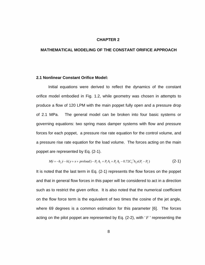
a pressure rise rate equation for the load volume. The forces acting on the main

poppet are represented by Eq. (2-1).

8

s L 23( ) 0.72 ( )y C C s s L L dMy b y k y x preload P A P A P A C h y P P= − − + + − + + − − (2-1)

It is noted that the last term in Eq. (2-1) represents the flow forces on the poppet

and that in general flow forces in this paper will be considered to act in a direction

such as to restrict the given orifice. It is also noted that the numerical coefficient

on the flow force term is the equivalent of two times the cosine of the jet angle,

where 69 degrees is a common estimation for this parameter [6]. The forces

acting on the pilot poppet are represented by Eq. (2-2), with ‘ ’ representing the F

input force from the actuator.

9

C L (2-2) 22( ) 0.72 ( )x dmx B x k y x preload C h x P P F= − − + + − − +

Equation (2-2) does not contain the pressure forces which act on each end of the

pilot poppet. For simplicity, initial efforts assume the pilot poppet is pressure

balanced while accounting for nonlinear damping forces by introducing an

artificial linear damping coefficient, xB , which represents the sum of linear and

nonlinear damping. It is noted that later efforts will introduce a more realistic

model of the forces acting on the pilot poppet. The change in control volume

pressure is given by Eq. (2-3). The assumption has been made that pilot poppet

movement has a negligible effect on the pressure of the control volume. This is

generally true due to the relatively small area and displacement of the pilot

poppet.

1 2(CC C

P Q QV A y

β= − +

−)CA y (2-3)

Realistically, load pressure is the pressure of the fluid contained between the

valve and a working piston cylinder assembly. Although later models incorporate

these dynamics, initial design is accomplished by replacing the piston cylinder

model with flow across a fixed orifice. The resulting model is shown in Eq. (2-4)

2 3 4(LL

P Q Q QVβ

= + − ) (2-4)

In order to simulate a particular pressure drops across the valve, the area of the

load orifice can be set as needed. The terms, Q1 through Q4, represent classic

orifice flow and are given be Eq. (2-5).

2dQ aC Pρ= Δ (2-5)

In cases where an orifice is variable, its area varies linearly with poppet position

with ‘h’ being the slope of the line.

2.2 Model Linearization:

Equations (2-1) through Eq. (2-5) represent a nonlinear model of the

forced feedback poppet as shown in Fig. 1.2. Although the nonlinear model is

more appropriate for examining valve behavior, a linear simplification and

accompanying tools provide means to better design the valve. In order to

achieve a linear model, the flow force terms, which are dependent on both

pressure and position, and the orifice equation, which depends on position and

the square root of pressure, are linearized about a nominal valve position.

Applying Taylor series expansion and neglecting higher order terms, the flow

force terms of Eq. (2-1) and Eq. (2-2) can be approximated by Eq. (2-6).

2 2(.72 ) (.72 )d O d Oflowforce C a P C h P displacementΔ + Δi i

(2-6) or flowforce kfc P kfq displacementΔ +i i

It is noted that displacement represents the distance the poppet has moved from

its nominal position while and represent conditions while the valve is at the

nominal position. A Taylor series expansion of the classic orifice equation results

in the linear approximation shown in Eq. (2-7).

0a 0P

10

( )01 22 2

dO d O

O

a CQ Q P hC P displacement

P ρρ

⎛ ⎞+ Δ + Δ⎜ ⎟⎜ ⎟Δ⎝ ⎠

i ii

12 Oor Q Q kc P kq displacement+ Δ +i i (2-7)

Substituting Eq. (2-6) into Eq. (2-1) and Eq. (2-2) while using nominal definitions

for displacements results in Eq. (2-8) and Eq. (2-9) respectively.

3 3 3( ) (y n n n L L L C C s s s O O )My b y k y x kfq y kfc P P A P A P A kfc P k x y preload= − − + − + + − + − − + + (2-8

) (2-9) 2 2( ) ( ) (x n n n C L O Omx B x k y x kfq x kfc P P F k x y preload= − − + − − − + − + + )

Changes in the size of the control volume will be neglected due the relatively

small displacements of y and x respectively. Substituting Eq. (2-7) into Eq. (2-3)

and Eq. (2-4) while assuming a nominal control volume results in Eq. (2-10) and

Eq. (2-11).

{ }12 1 2 1 2 12( ) ( )C c n C C L O O

COsP A y kq x kc P kc P P Q Q kc P

Vβ

= − − − − + − + (2-10)

{ }12 3 2 3 4 3 2 3 42( ) ( ) (L n n C L L L T s O O

L

P kq x kq y kc P P kc P kc P P kc P Q Q QVβ

= + + − − − − + + + − )O (2-11)

After choosing geometry, establishing a spring constant, and determining

supply and tank pressures it is possible to calculate nominal pressures and

hence to calculate the coefficients needed for the linear flow and flow force

equations. Under nominal conditions the main poppet only has static forces

acting on it and hence, neglecting flow forces, Eq. (2-1) reduces to Eq. (2-12).

(s s LO L O OCO

C

)P A P A k x y preloadPA

+ − + += (2-12)

Equation (2-2) reduces to Eq. (2-13) where is an arbitrary input to be chosen F

11

depending on the nominal position one wishes to study.

12

) ( O OF k x y preload= + + (2-13)

Static equilibrium of the each poppet also dictates that flow in equals flow out.

Examining the control volume gives 1Q Q2= , which after simplification becomes:

2

1

2(fix

LO CO s COO

aP P P P

a⎛ ⎞

= − −⎜ ⎟⎝ ⎠

)

4

(2-14)

Examining the load orifice gives 2 3Q Q Q+ = , which after simplification becomes:

2 2 2

2 3 42 2 2

2 3 4

CO O s fix TLO

O O fix

a P a P a PP

a a a

+ +=

+ + (2-15)

Given that and 2O Oa x h= 2 33O Oa y h= there are only four unknowns, ,

allowing Eq. (2-12) through Eq. (2-15) to be solved and the coefficients for the

linear model to be determined.

( , , ,CO LO O OP P x y )

CHAPTER 3

ITERATIVE ROOT LOCUS ANALYSIS AND DESIGN

3.1 Iterative Design Procedure:

Although the linearization in Chapter 2 requires geometry to be

established, a goal of this research is to use linear design tools to establish

geometric and other parameters that enhance valve performance. In order to

achieve this, an iterative procedure is utilized in which an initial linear model is

created and root locus plots serve as a guide to improving valve parameters. The

preliminary model is developed from flow requirements, basic physics, and trial

and error from nonlinear simulations until functional linearizations and root locus

plots are created. Root locus plots for various parameters, valve openings, and

pressure drops must be examined together and then a decision is made on

which parameter(s) to change in attempts to improve the stability, speed, and

damping of the system. After a constraint is changed, results can be examined

with nonlinear simulations and new linearizations can be created. New

linearizations give rise to a new set of root locus plots and the procedure is

repeated until valve performance meets necessary objectives.

To begin the iterative procedure the linearized system is rewritten in state

13

space form so as to be conducive to creating root locus plots. Removing all

terms from Eq. (2-8) through Eq. (2-11) which do not contain dynamic variables

or the input force results in equations which represent deviations from the

nominal conditions. The final deviation equations can be written in state-space

form as presented in Eq. (3-1).

0 1 0 0 0 0( ) ( )3 30 0

00 0 0 1 0 00( )2 2 20 1

00 0 ( )3 2 2 3 4 20

0 ( ) 0 ( )2 2 1 2

bk kfq kfc A Aky L cM M M M M

bk kfq kfc kfck xX Xm m m m m mkq kq kc kc kc kc

V V V VL L L L

A kq kc kc kccV V V Vco co co co

β β β β

β β β β

⎡ ⎤⎢ ⎥−− − + −−⎢ ⎥

⎡⎢ ⎥⎢⎢ ⎥⎢⎢ ⎥−− − −− ⎢⎢ ⎥= +⎢ ⎥

⎢ ⎥−⎢ ⎥+ +⎢ ⎥ ⎣⎢ ⎥− −

+⎢ ⎥⎢⎢ ⎥⎥⎣ ⎦

yyxu where X ux

PLPC

δδδ fδδ

δδ

⎤ ⎡ ⎤⎥ ⎢ ⎥⎥ ⎢ ⎥⎥ ⎢ ⎥=⎢ ⎥ ⎢ ⎥

⎢ ⎥ ⎢ ⎥⎢ ⎥ ⎢ ⎥⎢ ⎥ ⎢ ⎥⎣ ⎦⎢ ⎥⎦

=

)

(3-1)

A program is written that calculates the eigenvalues or roots of the “system

matrix” while one parameter is varied within a loop. In particular, root locus plots

are examined for the area of orifice one, the slopes for orifice two and three, the

spring rate, and the damping coefficient on the pilot poppet. It is thought that

poppet valve instabilities often arise when the main poppet is just cracked open

and hence the bulk of linearizations are for conditions in which the main poppet is

open a half a millimeter or less. In an attempt to uncover various performance

problems with the valve, separate linearizations are created for different

pressure scenarios including: ( 35 35sP MPa P MPa= Δ ≈ , ( 35 , 1s )P MPa P MPa= Δ ≈ ,

( 21 , 2.1s )P MPa P MPa= Δ ≈ , and ( 2.1 , 1s )P MPa P MPa= Δ ≈ where S LP P PΔ = − .

3.2 Root Locus Plots for the Constant Orifice Model:

Fig. 3.1 through Fig. 3.6 show root locus plots for linearizations where the

14

input force to the pilot poppet is 5 N and the pressure drop across the valve is

approximately 2.1 MPa. The root locus moves towards the X with a triangle

around it as the parameter value is increased. In Fig. 3.4 through Fig. 3.6 the

two poles to the far left, which appear in Fig. 3.3, have been excluded as they

were relatively stationary and their removal significantly improved graph

readability.

Fig. 3.1 Root locus varying (inlet orifice area),1a ( 21 , 2.1 )

15

sP MPa P MPaΔ ≈ 5f N= =

Fig. 3.2 Zoom of the right portion of Fig. 3.1

Fig. 3.1 and Fig. 3.2 demonstrate that of the parameters examined, a variation in

a1 has the greatest impact on the position of the two left most poles as well as

the right most pole. Fig. 3.3 shows that the slope of the main poppet orifice may

have little impact on the systems poles while Fig. 3.4 establishes a connection

between the slope of the pilot orifice and system oscillation. Fig. 3.5 reveals that

if the spring rate is too low the valve will be unstable while if it is too high

excessive oscillation can occur.

Fig. 3.3 Root locus varying (main orifice slope), ( 23h 1 , 2.1 )

16


Fig. 3.4 Root locus varying (pilot orifice slope),2h ( 21 , 2.1 )sP MPa P MPaΔ ≈ 5f N= =

Fig. 3.5 Root locus varying k (spring rate), ( 21 , 2.1 )PasP MPa P MΔ ≈ 5f N= =

Fig. 3.6 Root locus varying xb (pilot damping), ( 21 , 2.1 )asP MPa P MPΔ ≈ 5f N= =

Finally, Fig. 3.6 displays a correlation between the damping of the pilot poppet

and the damping of the entire system. Caution is taken in making claims on

valve performance based on Fig. 3.1 through Fig. 3.6 due to the fact these root

locus plots originate from just one operating point. There is no reason to assume

the valve will behave the same under more extreme pressure drops or larger

nominal openings due to nonlinearity. Because of the large number of root locus

plots needed to examine the valve in various scenarios, only a select few will be

17

shown to demonstrate contrasting information to what is shown in Fig. 3.1

through Fig. 3.6.

Careful examination of the root locus plots from various valve openings

and pressure drops reveals that the complex roots and the left most real root, as

seen in Fig. 3.1 through Fig. 3.6, appear almost identical for different valve

openings when the pressure drop is held constant. Fig. 3.7 supports this

statement by displaying similar root movement to that of Fig. 3.5 even though the

valve is now open 3.5 mm instead of 0.5 mm. It should be noted that the root

locus path clustered around -10 in Fig. 3.5 has shifted to the left in Fig. 3.7 and

ends at approximately -180. Although five of the six roots appear nearly

independent of valve position they shift dramatically and even take different

shape as the pressure drop is varied. Fig. 3.8 is a root locus plot for the scenario

depicted in Fig. 3.1 and Fig. 3.2 with the only change being an increase in

pressure drop from 2.1 MPa to 35 MPa. Comparing these figures, one can see

that an increase in pressure drop results in a dramatic shift of all root paths. Fig.

3.9 can be contrasted with Fig. 3.5 and demonstrates that a higher pressure drop

results in a significantly different root locus plot as the spring constant is varied.

Both figures link a higher spring rate to more oscillation but Fig. 3.9 also

establishes that optimum performance at high pressure drops demands

increasing the spring rate.

18

Fig. 3.7 Root locus varying k (spring rate), ( 21 , 2.1 )

19


Fig. 3.8 Root locus varying a1 (inlet orifice area), ( 35 35 )sP MPa P MPaΔ ≈ 5f N= =

The real root that is located at approximately -10, in Fig. 3.1 through Fig. 3.6,

initially appears problematic as it hinders the system speed. The design

variables tested do not provide a means to adequately position the pole, but a

thorough examination of its movements reveals that this pole reflects the load

dynamics or the fifth state equation.

Fig. 3.9 Root locus varying k ( 35 35 )

20


Fig. 3.10 Root locus varying 4kc ( 21 , 2.1 )sP MPa P MPaΔ ≈ 5f N= =

Fig. 3.10 brings light to the dominant effect (pressure flow coefficient for the

load orifice) has on the location of this pole. In

4kc

Fig. 3.10 the right most pole

moves from -10 to -63 as increases. Although the root at -10 in 4kc Fig. 3.1

through Fig. 3.6 appears to make the system unacceptably slow, Fig. 3.10

suggests this may not be the case. is dependent on the load orifice area 4kc

which has been arbitrarily adjusted to achieve desired pressure drops across the

valve. The impact that or the entire fifth state equation has on the system

dynamics is also dependent on V

4kc

L (load volume) which again is an arbitrary

value. This information suggests ignoring this pole in performance comparisons

and indicates that the load model should be improved to examine its impact on

stability. Due to the realized limitations of the load model presented in Chapter 2,

Chapter 4 assumes load pressure is fixed while Chapter 5 further analyzes the

impact of a varying load pressure.

21

CHAPTER 4

VARIABLE ORIFICE VS CONSTANT ORIFICE MODELS

4.1 Equations for the Variable Orifice Model:

The constant orifice model, given by Eq. (2-8) through Eq. (2-11), can be

easily modified to create the variable orifice model, as shown in Fig. 1.1.

Equation (2-8) and Eq. (2-11) remain unchanged. Equation (2-9) must have

three additional terms to account for flow forces while Eq. (2-10) gains one term

to account for decreasing flow into the control volume as the pilot poppet opens.

It should be noted that both 1kq and 1kfq will be negative due to the negative

relationship between x and the area of orifice one. The variable orifice model is

then represented by Eq. (2-8), Eq. (2-11), Eq. (4-1), and Eq. (4-2).

22

12 1 1 2( ) ( ) ( )x n n n n C C L O Omx B x k y x kfq x kfq x kfc P kfc P P F k x y preload kfc P= − − + − + − − − + − + + + s (4-1)

{ }11 2 1 2 1 2 12( ) ( )c C n n C C L O O

COsP A y kq x kq x kc P kc P P Q Q kc P

Vβ

= + − − − − + − + (4-2)

4.2 Criteria for Constant Verses Variable Orifice Model Comparisons:

The iterative root locus procedure performed on the constant orifice model

is also employed to analyze the variable orifice model although root locus plots

are not shown. In order to make the clearest comparison between the constant

and variable orifice models, the scenarios presented in this chapter are designed

so each model has nearly the same bandwidth. The models have identical

values for the pilot damping term, BBx, and for the feedback spring rate, k. The

value used for BxB is based on damping measurements from existing valves while

k comes directly from root locus analysis. The slope on the main poppet orifice is

set so as to achieve a 120 LPM flow rate for a 2.1 MPa pressure drop when the

valve is fully open. Similar bandwidths are achieved by adjusting the geometry

for the inlet and outlet orifices to the control volume. Fig. 4.1 presents the area

functions of inlet and outlet orifices for both models.

0.00E+00

5.00E-07

1.00E-06

1.50E-06

2.00E-06

2.50E-06

3.00E-06

3.50E-06

4.00E-06

0 0.5 1 1.5 2 2.5

pilot position (mm)

orifi

ce a

rea

(m^2

)

3

outlet for COinlet for COoutlet for VOinlet for VO

Fig. 4.1 Control volume inlet and outlet orifices

When the pilot poppet is closed both valves have the same inlet orifice area and

when the pilot poppet is fully open their outlet area minus their inlet area is also

23

equal. It is important to note that in each case the pilot poppet has a deadband

of approximately 1 mm before the outlet area will become larger than the inlet

area. Fig. 4.2 displays the roots for both systems with load pressure fixed and a

2.1 MPa pressure drop across the valve, while Fig. 4.3 zooms in on the right

portion of Fig. 4.2.

Fig. 4.2 Roots for linearization with 2.1 MPa pressure drop and valve open 0.2 mm

Fig. 4.3 Zoom in for the roots on the right side of Fig. 4.2

The Bode diagram appearing in Fig. 4.4 is from nonlinear simulations of the main

24

poppet position. The solenoid input force is a sinusoid such that the low

frequency amplitude is 50% of the maximum poppet stroke. The system

bandwidth is approximately 11.7 and 12.5 Hz for constant and variable orifice

models respectively when the supply pressure is 21MPa and the load pressure is

20 MPa. Although it is not shown here, the bandwidth increases as the pressure

drop across the valve increases.

Fig. 4.4 Frequency response for both models ( 21 , 1s )P MPa P MPa= Δ =

4.3 Simulation Comparisons:

Fig. 4.5 displays the main poppet position for a step input force which is

applied from 0 to 0.2 seconds. This figure demonstrates that for extremely low

pressure drops the main poppet can open or close 6 mm in approximately 0.075

seconds. The response is well damped and shows no signs of instability. An

entirely different response appears in Fig. 4.6 when the pressure drop is

increased to 35 MPa. Both models result in overshoot and oscillation, but

oscillations for the constant orifice model do not drop off as quickly. It is also

25

interesting to note that the input force required to open the valve 6 mm has

changed significantly from that of Fig. 4.5.

Fig. 4.5 Main poppet position in response to step input force from 0-.2 s, F=50.2 N for variable

orifice, F= 51.4 for constant orifice ( 2.1 , 1sP MPa P MPa)= Δ =

Fig. 4.6 Main poppet position in response to step input force, F=48.8 N for variable orifice, F=

54.6 for constant orifice ( 35 , 35s )P MPa P MPa= Δ ≈ The primary explanation for the differences in input force required to open the

valve is linked to the flow force terms included in the model. As was stated

26

previously, the flow forces are dependent on pressure drop and orifice area, and

are assumed to act in a direction to close the given orifice. For the constant

orifice model, outlet flow from the control volume results in a force to close the

pilot poppet which the solenoid must act against. This means that as the pilot

opens further or as the pressure drop increases, the flow forces grow and so

must the solenoid force. The geometry choices of Fig. 4.1 establish that there

will always be more flow through outlet orifice of the constant orifice model for a

given pressure drop and valve opening. Fig. 4.7 presents the flows out of the

control volume for the main poppet responses of Fig. 4.6.

Fig. 4.7 Flow out of the control volume for main poppet response of Fig. 4.6

( 35 , 35sP MPa P MPa)= Δ ≈ In the case of the variable orifice model, there are two orifices having an impact

on the pilot poppet. The inlet orifice acts to open the pilot poppet while the outlet

orifice acts to close it. Due to this representation, the flow forces are partially

cancelled and are thought to help stabilize the pilot poppet. Fig. 4.8

27

demonstrates that overshoot and oscillation problems can be even more

exaggerated for the case when the main poppet is cracked less than 1 mm.

Fig. 4.8 Main poppet cracked open in response to step input force, F=8.1 N for variable orifice,

F=13.6 N for constant orifice ( 35 , 35sP MPa P MPa)= Δ ≈

4.4 Design Information Obtained from Model Comparisons:

Nonlinear simulations show that constant and variable orifice models can

be designed to have similar bandwidths, but there are trade offs between the two

models. In order to obtain similar bandwidths, the constant inlet orifice had to be

enlarged so it was equal to the maximum size of the variable inlet orifice and the

slope of the outlet orifice had to be increased in the constant orifice model. Fig.

3.2 indicates that performance can be reduced if the area of the inlet orifice is set

too large while Fig. 3.4 suggests that if the outlet orifice slope is too steep

oscillation may be a problem. Although it is not possible to determine direct

cause and effect, nonlinear simulations of Fig. 4.6 and Fig. 4.8 show increased

oscillation for the constant orifice model. In short, the constant orifice model

forces a compromise between designing for a stability margin and for system

28

bandwidth. In Fig. 4.1 through Fig. 4.8 the design focused on bandwidth while

Fig. 4.9, Fig. 4.10, and Fig. 4.11 show a constant orifice model design which is

focused on stability. These figures pertain to a model that has an outlet orifice

slope equal to that of the variable orifice model and the fixed inlet orifice which

has been reduced to 4.375e-7 m2. Fig. 4.9 demonstrates how a reduction in the

inlet orifice area can slow the closing of the main poppet. This increase in the

valve close time is due to a reduction of the pressure rise rate for the control

volume. When the solenoid is shut off, the spring force quickly closes the pilot

poppet, but the main poppet will not close immediately. The spring force is not

strong enough to counter the upward force on the main poppet due to supply

pressure.

Fig. 4.9 Main poppet response to a solenoid input force from 0-.2 s. Constant orifice model

modified for stability as compared to Fig. 4.5 ( 2.1 , 1s )P MPa P MPa= Δ = The pressure in the control volume must increase enough to force the main

poppet closed. This pressure rise rate is dependent on the size of the inlet

orifice and hence why a reduction in the inlet area impacts valve closing. It is

29

noted that the simulation in Fig. 4.9 is with a low pressure drop for the purpose of

examining the worse case scenario. At higher pressure drops the variable orifice

model continues to out perform the constant orifice model but with a decreasing

margin. Although Fig. 4.9 represents a decrease in performance it was also

claimed that geometry changes would trade performance for stability.

Fig. 4.10 Main poppet response to solenoid input force. Constant orifice model modified for

stability as compared to Fig. 4.6 ( 35 , 35sP MPa P MPa)= Δ ≈ Fig. 4.10 backs this claim by showing that the adjustments to the constant orifice

model reduced both oscillation and overshoot below that of the variable orifice

model. Finally, Fig. 4.11 presents the change in system bandwidth that results

from attempts to increase the stability margin of the constant orifice model. In

particular it is shown that the bandwidth drops from approximately 11.7 to 6 Hz.

30


( 21 , 1sP MPa P MPa)= Δ =

31

CHAPTER 5

EXAMINATION OF PREVIOUSLY UNMODELED DYNAMICS

5.1 An 8-State Model:

Bode plots and nonlinear simulations, presented in Chapter 3 and Chapter

4, compare constant and variable orifice models for five-state systems, while the

original root locus plots depended on a 6-state model. Although useful

comparative results could be extracted, it is important to expand the system to

examine the validity of the assumptions made. In particular, this chapter will

study the effects of improved load dynamics and nonlinear damping on the pilot

poppet. The original load orifice will be replaced with a piston/cylinder assembly

and the artificial linear damping of the pilot poppet will be replaced by pressure

forces acting on its ends and flow through its central tube. The new model will

contain eight states: the main poppet position and velocity ( ), the pilot poppet

position and velocity (

,y y

,x x ), the control volume pressure between the two

poppets ( ), the control volume pressure above the pilot poppet (CP PP ), the load

volume pressure ( ), and the velocity of the load piston ( ). The main control

volume is connected to the pilot poppet control volume via the tube located in the

center of the pilot poppet. It is assumed that classic laminar tube flow will exist

LP z

32

between the two control volumes as presented in Eq. (5-1).

4

6 (8 C P

pilot

RQ PL

πμ

= )P− (5-1)

The artificial damping term, xB , is replaced by a more realistic linear damping

coefficient, xb . In linearizing the model, the assumption is made that variations in

each control volume size can be neglected. The piston/cylinder assembly is

modeled as a simple mass-damper system with load pressure acting on the head

end of the piston and an external load force acting on the rod end. In this

scenario, the load force, , can be adjusted to provide desired pressure drops

across the valve. Both the constant and variable orifice models are expanded to

eight states although the results are only shown for the variable orifice model. It

is also important to note that from Chapter 5 onward, all results presented will

make use of an 8-state model with the parameters given in the appendix.

Equation (5-2) through Eq. (5-7) represent the nonlinear variable orifice model

while Eq. (5-8) represents the linear equations written in state space form.

loadF

23( ) .72 (y C C s s L L d )s LMy b y k y x preload P A P A P A C h y P P= − − + + − + + − − (5-2)

(5-3) 2 2

1 1max 2

( ) ( )

.72 ( )( ) .72 ( )x pilot C p

d s C d C

mx b x k y x preload A P P

C h x a P P C h x P P F

= − − + + − −

+ + − − − L +

1 2(cC C

P Q QV A y

)cA yβ= − +

− (5-4)

6(P pilotpilot pilot

P QV A x

)A xβ= −

+ (5-5)

33

2 3(LLoad pist

P Q QV A z

)pistA zβ= +

+− (5-6)

pist L pist z loadM z P A b z F= − + (5-7)

3 3

1 22 1 2

1 2 1 2 20 0 0 0

0 0 0

3 2 20 0 0

0 1 0 0 0 0 0 0

0 0

0 0 0 1 0 0 0 0

0 0

0 ( ) 0 ( ) 0

0 0 0 0 0

0 0

y c L

p ilo t p ilo tx

CC C C C

p ilo tP P P

L L L

bk kfq A kfc AkM M M M M

kfc kfc A Abk kfq k fq k fckm m m m m m

A kq kq kc kc kcX V V V V

A kcp kcpV V V

kq kq kcV V V

β β β β

β β β

β β β

−− − − +−

− − −−− − +−

−− +=

− −

0

0

2 30 0

0 ( )

0 0 0 0 0 0

000

1

0000

p is tL L

p is t z

p is t p is t

C

P

L

X

kc kc AV V

A bM M

yyxxm u X u f

PPPz

β β

δδδδ

δδδδδ

⎡ ⎤⎢ ⎥⎢ ⎥⎢ ⎥⎢ ⎥⎢ ⎥⎢ ⎥⎢ ⎥⎢ ⎥⎢ ⎥⎢ ⎥⎢ ⎥⎢ ⎥⎢ ⎥⎢ ⎥⎢ ⎥−

+⎢ ⎥⎢ ⎥⎢ ⎥−⎢ ⎥⎢ ⎥⎢ ⎥⎣ ⎦

⎡ ⎤ ⎡ ⎤⎢ ⎥ ⎢ ⎥⎢ ⎥ ⎢ ⎥⎢ ⎥ ⎢ ⎥⎢ ⎥ ⎢ ⎥⎢ ⎥ ⎢ ⎥+ = =⎢ ⎥ ⎢ ⎥⎢ ⎥ ⎢ ⎥⎢ ⎥ ⎢ ⎥⎢ ⎥ ⎢ ⎥⎢ ⎥ ⎢ ⎥⎢ ⎥ ⎢ ⎥⎣ ⎦⎢ ⎥⎣ ⎦

(5-8)

5.2 Validation of 8-State Model Linearization:

The linear model of Eq. (5-8) is not only used to verify claims made with

the 5-state model, but is also used in Chapter 6 in efforts to create a system

observer. The accuracy of an observer depends on accuracy of the model it

employs. For this reason and as a general check on mathematical efforts thus

far, simulations are run side by side for both the linear and nonlinear models.

Fig. 5.1 through Fig. 5.8 show that the linear model provides an excellent

approximation of the nonlinear model for all 8 states in response to a unit step

input.

34

Fig. 5.1 Main poppet position for a unit step input

Fig. 5.2 Main poppet velocity for a unit step input

Fig. 5.3 Pilot poppet position for a unit step input

35

Fig. 5.4 Pilot poppet velocity for a unit step input

Fig. 5.5 Control volume pressure for a unit step input

Fig. 5.6 Pilot control volume pressure for a unit step input

36

Fig. 5.7 Load volume pressure for a unit step input

Fig. 5.8 Load piston velocity for a unit step input

5.3 8-State vs. 5-State Model:

In Chapter 3 a decision was made to replace a restrictive load orifice

model with a fixed load pressure. The assumption was made that arbitrary

settings on both the load orifice and load volume were introducing an extraneous

root at -10. Fig. 5.9 displays the roots of the expanded system and the 5-state

system for a 2.1 MPa pressure drop. It is noted that the extremely fast root

(-326,000) associated with PP has been removed from the graph for readability.

37

Fig. 5.9 Roots for linearization with valve open 0.2 mm ( 21 , 2.1s )P MPa P MPa= Δ ≈

Fig. 5.10 provides more information about how the poles have moved between

the 5-state and 8-state models. In general the 8-state model appears to have

faster roots but careful analysis determines that the imaginary poles at

are due to the variable load pressure and the load piston dynamics.

While the load pressure is not creating an extremely slow root at -10 as early

results suggested,

155 463i− ±

Fig. 5.10 suggests that load dynamics can impact system

performance and stability.

Fig. 5.10 Zoom in for the right side of Fig. 5.9

38

Again, it is imperative to remember that poles presented here are for a

linearization at only one set of operating conditions. Although not shown here,

nonlinear simulations and linearizations for an array of operating conditions

support that the system is stable with nonlinear damping and tube flow through

the pilot poppet. Examination of the Reynolds number for flow through the pilot

poppet does show spikes above 2100 which is in violation of Eq. (5-1) [16]. The

spikes in the Reynolds number occur when the pilot poppet rapidly accelerates

from a zero velocity due to the solenoid or spring forces. It is possible that flow

will transition from laminar to turbulent, and that the pilot poppet will not move as

quickly as the model indicates. The assumption is made that this will not

seriously degrade system performance and that the model captures the

important dynamics.

The 8-state model predicts, as is expected, that system performance is

degraded under extreme load forces or low pressure drops while it shows more

oscillation at high pressure drops. In order to validate that the 8-state model

meets performance requirements, Fig. 5.11 again presents a Bode plot created

from nonlinear simulations.

39


( 21 , 1sP MPa P MPa)= Δ = These results suggest that a variable load pressure as opposed to a fixed load

pressure has only a small impact on the system bandwidth. As a whole, the

results from the 8-state model indicate that the 5-state model includes the

important performance characteristics of the system but neglects stability

concerns that may arise from the interaction with load dynamics.

40

CHAPTER 6

MECHANICAL AND ELECTRONIC CONTROL DESIGNS

6.1 Introduction to Flow Control:

The first phase of this research was to design a forced-feedback metering

poppet valve which meets open loop performance requirements for the main

poppet position. The second phase focuses on methods to control flow across

the valve. Flow is dependent on both poppet position and pressure drop across

the valve which leads to two methods for achieving flow control. The first method

is to use a mechanical pressure compensator to maintain a desired pressure

drop across the valve while the operator adjusts the poppet position as needed to

provide the desired flow. Although valve design shown in Fig. 1.1 and Fig. 1.2

provides no means to attach a compensator, mathematical modeling makes the

assumption that it is possible. The second method of flow control is to allow

pressure drop to vary freely and then establish the poppet position as a function

of both desired flow and measured pressure drop. This method entails the use of

electronic control and feedback of pressure drop across the valve. Several

electronic control designs will be presented while mechanical pressure

compensation will serve as a benchmark for performance.

41

6.2 Mechanical Pressure Compensation for Flow Control:

The mechanical pressure compensator is a pre-compensator with a

restriction on supply side pressure. The model consists of a typical spring mass

damper system which affects the size of a variable orifice between supply

pressure, sP , and the compensated supply pressure, ,s cP .

Fig. 6.1 System with compensator, metering poppet valve, and load The compensator is implemented in the system as shown in Fig. 6.1 while it is

mathematically represented by Eq. (6-1), Eq. (6-2), and Eq. (6-3).

(6-1) ,comp comp comp comp comp comp L comp s c comp c prem x k x b x P A P A F= − − + + ,

, (s c compcomp

P QV 3)Qβ

= − (6-2)

,2 (comp comp d s s cQ a C P Pρ

= )− (6-3)

Assuming supply pressure is at least 2 MPa higher than load pressure, the

compensator is designed to maintain approximately a 2 MPa pressure drop

across the metering poppet valve. Fig. 6.2 displays nonlinear simulation results

for both the constant and variable orifice models with pressure compensation. In

42

these simulations the input was set to achieve a desired flow of 30 LPM while

supply pressure was constant and the load pressure varied as much as 1GPa/s.

Fig. 6.3 is a profile of the difference between supply pressure and load pressure.

Fig. 6.2 Valve flow for pressure compensated models (desired flow 30LPM)

Fig. 6.3 Pressure drop from supply to load pressure

Fig. 6.2 provides expected results for mechanical pressure compensation. For

the first 0.1 seconds the pressure drop is near 2MPa and therefore there is no

pressure compensation. The variable orifice model settles to steady state slightly

43

faster than the constant orifice model in agreement with previous results. At 0.1

seconds the load pressure begins to fall approximately 1 GPa/s. The flow quickly

spikes as the compensator lags behind but then settles to 33 LPM. When the

load pressure rises at 0.2 seconds, the compensator again lags behind but

opens fully and flow settles to 19 LPM. The final pressure drop is near 0.9 MPa

which is below the compensators designed pressure drop and therefore high

steady state error results. Due to the similar results between the two models,

plots of electronic control schemes will only be contrasted with the compensated

variable orifice model.

6.3 Electronic Flow Control:

6.3.1 Table Look-up Control:

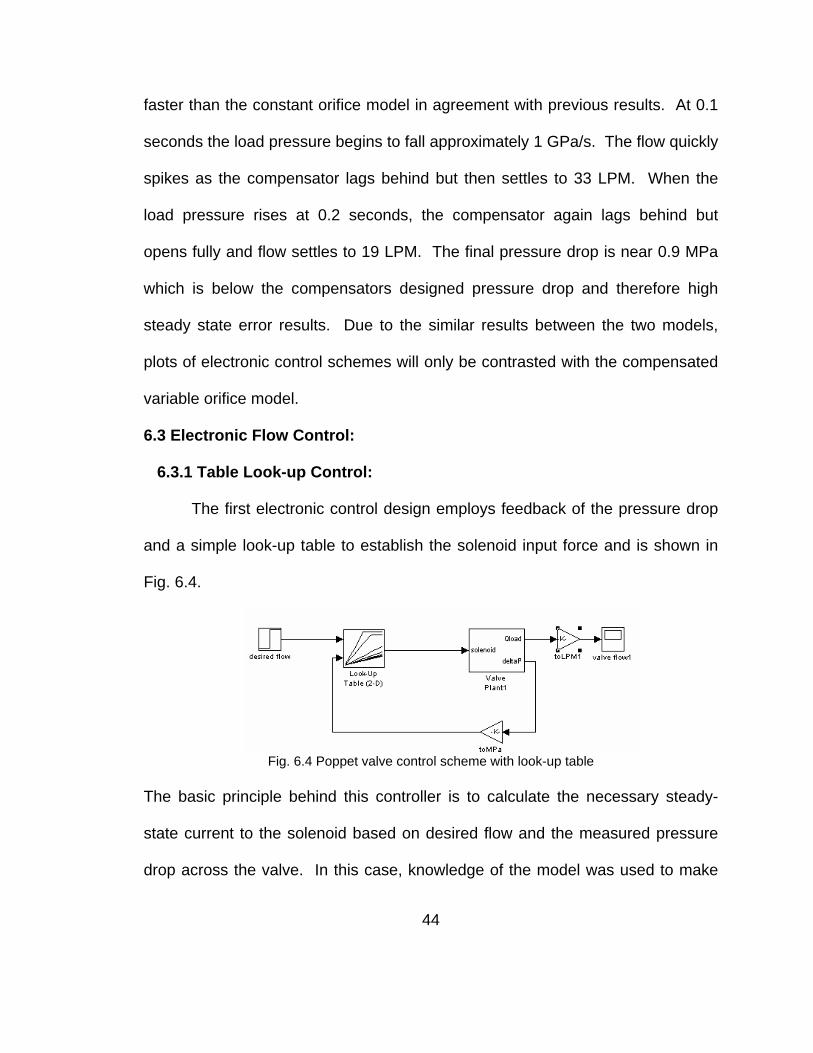
The first electronic control design employs feedback of the pressure drop

and a simple look-up table to establish the solenoid input force and is shown in

Fig. 6.4.

Fig. 6.4 Poppet valve control scheme with look-up table

The basic principle behind this controller is to calculate the necessary steady-

state current to the solenoid based on desired flow and the measured pressure

drop across the valve. In this case, knowledge of the model was used to make

44

approximate linear relationships between flow and solenoid force for a small

array of pressure drops. The best controller of this type would be designed by

creating a very precise look-up table based on actual tests of a sample of

production valves. Fig. 6.5 and Fig. 6.6 provide nonlinear simulation results

using the controller shown in Fig. 6.4. Simulations are run for desired flows of 30

and 110 LPM and the results are compared with mechanical pressure

compensation. Again, it is noted that the constant orifice model as it appears in

control design figures is the design which focuses on stability and not

performance. For a 30 LPM flow, the simulation results appear similar although

when the pressure drop becomes less than 2 MPa the mechanical compensator

provides a much higher steady-state error.

Fig. 6.5 Look-up table control vs. pressure compensation, desired flow 30 LPM, see Fig. 6.3 for

pressure drop The mechanical pressure compensator has no means to achieve the desired flow

when the pressure drop falls below its design value while electronic control can

open the valve further to minimize steady-state error. In Fig. 6.6 steady-state

45

error is similar even under low pressure drops because the valve eventually hits

its endstop. The results for the transient response are significantly different for

high flow compared to low flow. For a 30 LPM flow the percent overshoot is

comparable for all models, while for 110 LPM flow, the pressure compensator

provides a much smaller spike in flow in response to the sudden drop in load

pressure.

Fig. 6.6 Look-up table control vs. pressure compensation, desired flow 110 LPM, see Fig. 6.3 for

pressure drop

Although Fig. 6.5 and Fig. 6.6 indicate that the constant orifice model has the

highest percent overshoot this is not always the case. In Fig. 6.7 and Fig. 6.8 the

desired flow is varied over time while the pressure drop is relatively stable. The

load force is held constant at appropriate values so that pressure drop is near 30

MPa in Fig. 6.7 and 1 Mpa in Fig. 6.8. For high pressure drops the variable

orifice model with table look-up control has the highest overshoot and oscillates

more than the other models while the constant orifice model actually has the

46

fastest settling time. For low pressure drops, all models show over damped

responses but the variable orifice model has the fastest settling time.

Fig. 6.7 Varying desired flow between 10 and 100 LPM, pressure drop approx 30MPa

Fig. 6.8 Varying desired flow between 10 and 70 LPM, pressure drop approx 1 MPa

In general, as pressure drop decreases, the constant orifice model falls behind

the performance of the variable orifice model. Control of the constant orifice

model becomes limited by its poor open loop performance at low pressure drops.

Steady-state error for electronic control models appears to vary more at low

47

pressure drops but this is direct result of simplifications in look-up tables. If the

look-up tables are made more accurate, steady-state error should be identical for

both models. Trade offs in using mechanical pressure compensation are

demonstrated by its comparatively slower response at high pressure drops and

its high steady state error at low pressure drops. High steady-state error is

somewhat misleading in that an operator will intuitively provide a controlling

response when the machine operates at this condition.

6.3.2 Table Look-up with PD Control:

The next electronic controller, shown in Fig. 6.9, seeks to enhance

performance by combining look-up table control with proportional derivative (PD)

control. It is noted that integrator control is not included in this work primarily due

to slowness of response. Simulations which examined integrator control resulted

in settling times that were typically more than an order of magnitude greater than

when the integrator was not included. Because some steady-state error was

deemed acceptable, work proceeded with only PD control.

Fig. 6.9 Electronic control with look-up table and PD control

48

The controller shown in Fig. 6.9 feeds back pressure drop and valve flow. While

pressure drop is still an input to the original look-up table, the flow feedback is

used to establish a flow error signal which is incorporated into PD control. The

proportional gain on the flow error signal can shorten the transient response

while the derivative gain can be used to minimize overshoot. An additional

benefit of this type of controller is that inaccuracies contained in the look-up table

will be compensated for by gains on the flow error signal. Although a look-up

table can be designed using test data, each valve will be unique and will perform

differently as it shows wear. A drawback of using PD control on the flow error

signal is that it requires having knowledge of the flow across the valve. This

could be done either measuring flow directly or measuring the main poppet

position and then calculating flow based on position and pressure drop. An

observer design will also be considered in section 6.5 as a means of estimating

flow using pressure measurements.

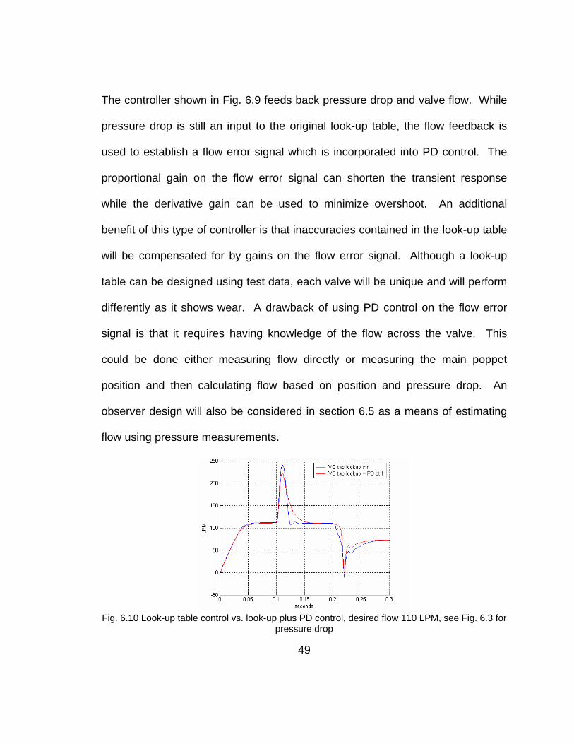
Fig. 6.10 Look-up table control vs. look-up plus PD control, desired flow 110 LPM, see Fig. 6.3 for

pressure drop

49

Fig. 6.10 indicates that the addition of PD control reduces the spike in flow due to

the sudden decrease in load pressure. Note that Fig. 6.10 and subsequent

figures use table look-up control as shown in Fig. 6.4 as a benchmark for

additional control designs. The constant orifice results are dropped from the

figures because their inclusion only provides redundant information seen in

previous figures. Fig. 6.11 and Fig. 6.12 display results for simulations where the

load force is fixed while desired flow is varied at 0.1 and 0.3 seconds.



50

Results indicate that combining the look-up table with PD control reduces steady

state error and provides damping to the transient response but does not reduce

settling time.

6.3.3 Gain Scheduled PD Control:

The gains for the constant PD control shown in Fig. 6.9 were chosen by

trial and error, but examining the root locus plots for the closed loop system with

negative feedback suggests that the system could benefit from gain scheduling.

Root locus plots are generated using the A and B matrices from Eq. ((5-8) while

the C and D matrices come from Eq. (6-4), where the output is flow.

[ ]3 2 2 2 30 0 0 ( ) 0Y kq kq kc kc kc X u= − − 0+ (6-4)

Fig. 6.13 indicates that for high pressure drops the controller gain should be kept

as small as possible to minimize overshoot and oscillation. Fig. 6.14

demonstrates that for low pressure drops increasing the controller gain can

increase the system bandwidth without significantly jeopardizing overshoot or

oscillation. In particular it is noted that the system would benefit from a control

gain of at 1 MPa pressure drop while the same gain would cause the

system to be unstable at a 35 MPa pressure drop.

42 10×

51

Fig. 6.13 Root locus for negative feedback of flow (35 MPa pressure drop)

Fig. 6.14 Root locus for negative feedback of flow (1 MPa pressure drop)

Knowledge gained from root locus plots lead to the control design shown in Fig.

6.15. This control scheme creates a flow error signal in LPM and then converts

it to meters cubed per second before entering the PD controller. As the pressure

drop increases the proportional and derivative gains are decreased. The gain

scheduling is contained in a simple linear look-up table and was tuned by trial

and error to adjust damping and achieve acceptable steady-state error.

52

Fig. 6.15 Gain scheduled PD controller based on measured pressure drop

Fig. 6.16 shows that gain-scheduled PD control results in a smaller spike in flow

as load pressure drops, as compared to look-up table control.

Fig. 6.16 Look-up table control vs. gain scheduled PD control, desired flow 110 LPM, see Fig. 6.3

for pressure drop Fig. 6.17 shows that gain-scheduled PD control can be used to reduce oscillation

at high pressure drops but Fig. 6.17 and Fig. 6.18 also emphasize that this

control method is not the best for minimizing steady-state error.

53



6.3.4 Table Look-up with Gain Scheduled PD Control:

The final controller that is examined employs both a look-up table and

gain-scheduled PD control. The block diagram for this controller is shown in Fig.

6.19. Again, the gains for the PD control decrease as the pressure drop

decreases but when the table look-up is included the gains are reduced so that

the PD control effort is much smaller.

54

Fig. 6.19 Gain scheduled PD control with look-up table

Fig. 6.20 displays the response to changes in load pressure when desired flow is

set to 110 LPM. Fig. 6.21 simulates changing the desired flow when the

pressure drop is high, while Fig. 6.22 presents a similar simulation for the case of

a low pressure drop. The effort with gain-scheduled PD control results in smaller

transient spikes and less oscillation, as expected. In comparison with Fig. 6.17

and Fig. 6.18, gain scheduling the PD control effort provides a reduction in

steady-state error.

Fig. 6.20 Look-up table control vs. look-up table with gained PD control, desired flow 110 LPM,

see Fig. 6.3 for pressure drop

55



6.4 Flow Control Summary:

In efforts to maintain flow across the metering poppet valve, mechanical

pressure compensation and four electronic controllers are presented and

compared. A mechanical pressure compensator is best able to manage flow in

response to extreme drops in the load pressure while it is the worst at minimizing

steady-state error. The simplest electronic controller uses feedback of pressure

56

drop and a look-up table to drive the valve to the desired steady-state flow. The

look-up table results in differing steady-state error as operating conditions vary

but much of this error can be eliminated by refining the look-up table to include a

larger array of pressure drops. At high pressure drops, the look-up table

approach allows oscillation to occur but the system still responds quickly. The

three remaining electronic controllers incorporated PD efforts on a flow error

signal. The first, which combined constant PD control with the look-up table, was

able to reduce transient spikes, provide damping, and reduce steady-state error.

The second, which removed the look-up table and gain scheduled PD efforts

based on pressure drop, was able to reduce transient spikes and provide

damping but resulted in higher steady-state error. The last, which combined gain

scheduled PD efforts with a look-up table, was able to reduce transient spikes

and provide damping while leading to the lowest steady-state error.

6.5 Observer Design:

The majority of electronic controllers presented in this research employ

feedback of valve flow. To avoid the cost of additional sensors it is

advantageous to use the valve model to provide real time state estimates which

can be used to calculate a flow estimate. Steps are taken here to create an

observer which is limited to constant load force conditions. If results are positive,

the methods undertaken will be useful in expanding the observer to function

under all operating conditions.

The basic principle of an observer is that a model of the system should be

57

able to predict the transient states of the valve. The observer does not have

knowledge of the real time initial conditions of the valve and so it makes use of

real time measurements to synchronize itself with the system. In simple terms,

the real system control effort is input to the valve model which mathematically

responds and predicts the states. Lack of initial conditions means the model will

be in error but real time measurements provide the observer knowledge of its

error so that it can correct itself. In the case of the metering poppet valve, the

error signal between estimated load pressure and measured load pressure is

multiplied by a gain to synchronize model estimates with real time states.

Observer design typically makes use of a state-space model of the system.

In this case the A and B matrices come from Eq. (5-8) while the measurement or

output matrix, [ ]0 0 0 0 0 0 1 0C = , and D = 0. The observer provides

estimates of the ‘true’ states based on Eq. (6-5)

[ ]ˆ ˆ( )e

uX A K C X B K

Ye⎡ ⎤

= − + ⎢ ⎥⎣ ⎦

(6-5)

ˆeY = load pressure measurement K = error gain matrix X = state estimates

Existing computer algorithms can typically calculate the matrix , given A, C and

the desired estimator poles for the system [17]. Two difficulties are realized in

this process. First, the system poles are not easily moved to any location but

must be moved far enough to the left in the complex plane to ensure that the

observer dynamics decay several times faster than the plant dynamics. A

eK

58

feasible set of closed loop poles is found by considering the eigenvalues of the

original A matrix and multiplying the real part by a factor of 8 and the imaginary

part by a factor of 0.3. The second numerical difficulty arises due to a poorly

scaled state-space system. In order to calculate the estimator gain matrix, , it

is necessary to perform a matrix transformation on the system such that

eK

transformX TX= . The transformation allows for numerical calculation of

which can then be converted to by calculating . ,e transformK eK 1,e transformT K−

Once observer gains are calculated, simulations can be run to verify that

the state estimates are able to quickly track the ‘true’ states. Performance

requirements indicate that commanded valve flow must have a settling time of

0.1 seconds or less. This requirement indicates that an observer must be able to

track actual flow in a small fraction of the demanded settling time. The

comparison of observer estimates verses the ‘true’ states are shown in Fig. 6.23

through Fig. 6.30.

Fig. 6.23 Observer estimate of main poppet position

59

Fig. 6.24 Observer estimate of main poppet velocity

Fig. 6.25 Observer estimate of pilot poppet position

Fig. 6.26 Observer estimate of pilot poppet velocity

60

Fig. 6.27 Observer estimate of pressure above main poppet

Fig. 6.28 Observer estimate of pressure above pilot poppet

Fig. 6.29 Observer estimate of load pressure (measured)

61

Fig. 6.30 Observer estimate of load piston velocity

Fig. 6.23 through Fig. 6.30 show that the observer tracks the ‘true’ states in less

than 0.02 seconds for all cases except and PP x . Although faster tracking is

desired, it is thought that 0.02 seconds will be adequate to provide desired

performance. Past work comparing linear and nonlinear models indicates that

better tracking should be obtained for and PP x but it is thought this problem may

arise due to the pole associated with originally falling near -326,000 rad/s.

Although tracking for and

PP

PP x is not achieved this does not interfere with the

ultimate goal of estimating flow. Equation (6-4) demonstrates that flow is not

dependent on either or PP x and therefore the observer designed will be

adequate. Fig. 6.31 displays ‘true’ flow against the estimate of flow calculated

from observer state estimates. These results suggest that a simpler model could

be used for observer design in which the pilot poppet can be represented

mathematically as was done in the 5-state model.

62

Fig. 6.31 Observer flow estimate vs. ‘true’ flow

63

CHAPTER 7

ROBUST CONTROL ANALYSIS

7.1 Introduction to Robust Analysis:

All control designs presented in this work are dependent on the accuracies of

the valve models used. A true test of any control scheme requires implementing

the controller on actual hardware. Although no hardware is available, an

appropriate first step is to provide a robust control analysis. A robust control

analysis will seek to determine if the system will remain stable and meet

performance criteria even when the valve model is in error. This is done by

examining the valve model and establishing which parameters and dynamics are

most likely to be in error. Establishing error bands for parameters in the system

provides a means to model uncertainty. Once an uncertainty model is

calculated, it is possible to test for stability and performance under worst case

conditions.

In particular, a robust control analysis is provided for the controller pictured in

Fig. 6.9. Analysis of system performance will include examining nominal

performance, NP, robust stability, RS, and robust performance, RP, as presented

by Skogestad [18]. NP, RS, and RP criteria as presented here after are

64

dependent on the assumption that the valve control system is nominally stable.

Although nominal stability has not been proven, this assumption is consistent

with all modeling results that have been observed thus far.

7.2 Nominal Performance and the Sensitivity Transfer Function:

If a system is nominally stable it is then a logical next step to prove that

NP is achieved. The sensitivity function, “S”, the transfer function between the

error signal and the reference input, is a good indicator of the closed-loop system

performance. An upper bound transfer function, 1/ ( )PW s can be placed on the

magnitude of “S” to verify that a given set of performance criteria is met.

is a performance weighting function given by Eq. (7-1) where lower case “ s ” is

the Laplace variable, “

( )pW s

M ” is maximum high-frequency error set equal to 2, “ bω ”

is the desired system bandwidth set equal to 50.24 rad/s, and “ A ” is the

maximum steady-state error set equal to 0.1.

bp

b

s +MW (s)=s+ A

ω

ω (7-1)

Mathematically stated, |S| will meet performance requirements if the inequality in

Eq. (7-2) is satisfied.

( )S 1pNP W s ω⇔ < ∀ (7-2)

In order to present results for Eq. (7-2), the sensitivity transfer function must be

determined from Fig. 6.9. To simplify the calculation of S, the pressure drop will

65

be assumed constant and therefore its feedback connected to the look-up table

can be removed. This leaves negative flow feedback and a feedforward path

which is only a function of the reference input. The simplified block diagram is

shown in Fig. 7.1.

Fig. 7.1 PD/table look-up control with pressure drop held constant

Linear superposition makes it possible to break the two reference input paths of

Fig. 7.1 into the two separate block diagrams shown in Fig. 7.2.

1nom

( ) 1( ) 1+KG

E sSR s

= =

f nom2

nom

( ) -K G( ) 1+K G

E sSR s

= =

Fig. 7.2 Block diagram reduction for calculating sensitivity transfer function

66

1S plus from 2S Fig. 7.2 gives the final system sensitivity shown in Eq. (7-3)

f nom

nom

1 K GS1 G K−

=+

(7-3)

Here, K represents the transfer function for the PD control effort, is a constant

pressure slope from the look-up table, and G

fK

nom is the transfer function for the

linearized valve system. Because the above derivation of “S” assumes the

pressure drop is constant, effects of pressure variation must be accounted for by

analyzing an array of controllers. “S” is calculated for three different nominal

plants with pressure drops of 1 MPa, 2.1 MPa, and 35 MPa. Fig. 7.3 plots on a

logarithmic scale for all three pressure drops. Because SPW is less than 1 for all

operating frequencies nominal performance is achieved for the tested pressure

drops.

Fig. 7.3 Nominal Performance for 3 pressure drops when the valve is cracked open

7.3 Derivation of Robust Stability with Multiplicative Uncertainty:

67

To analyze robust stability, possible errors in the valve model must be

considered as was discussed in section 7.1. This error will be considered by

building multiplicative uncertainty into the model as is shown in Fig. 7.4.

Δ

Fig. 7.4 Control scheme with multiplicative uncertainty included

The symbol is the set of stable transfer functions whose magnitude is less

than or equal to one, while is the transfer function for the upper bound on

uncertainty and is given by Eq.(7-4). Here G

Δ

IW

p is the perturbed valve plant due to

variation in system parameters (See sect 7.4 for calculation of Gp).

p nom

nom

G ( ) G ( )( )

G ( )I

s sW s

s−

≥ (7-4)

After multiplicative uncertainty is included in the system, Fig. 7.4 can be redrawn

as Fig. 7.5 through basic block diagram reduction.

Δ

N

Fig. 7.5 NΔ configuration for determining RS criteria

Assuming nominal stability and applying the Nyquist stability condition to Fig. 7.5,

68

RS is achieved if and only if the loop transfer function NΔ does not encircle -1

for all . Mathematically this criterion can be shown to reduce to Eq. (7-5). Δ

( ) 1RS N s ω⇔ < ∀ (7-5)

To find , the block diagram in ( )N s Fig. 7.4 is reconfigured with “from delta” being

the new system input and “to delta” being the new system output. The goal is to

determine if there is instability due to , therefore the flow output and the

reference input paths can removed due to the NS requirement. The resulting

block diagram manipulation is presented in

IW

Fig. 7.6 where the upper right most

block represents . ( )N s

( )N s

nom

nom

KG1 KG

IW−+

Δ

Fig. 7.6 Block diagram for determining robust stability criterion

Substituting the result of Fig. 7.6 into Eq. (7-5), the RS criterion now can be

written as Eq. (7-6).

nom

nom

KG 11 KG

IWRS ω−⇔ < ∀

+ (7-6)

7.4 Multiplicative Uncertainty Weighting Function WI:

The final step in the robust stability analysis is to establish as given by IW

69

Eq. (7-4). This is done using a computer algorithm to calculate possible as

the plant is perturbed from the nominal model. Nested ‘for’ loops are used to

vary uncertain plant parameters as they appear in the state matrix, Eq. (5-8).

The following uncertainties are introduced as plant perturbations:

IW

30%β ± ,

, , and k 5%± dC 10%± Zb 20%± . In particular, the bulk modulus can vary due to

entrained air or temperature changes, the spring constant is dependent on

manufacturing tolerances, the orifice coefficient is known to vary with geometry

and viscosity, and finally friction is always a parameter which is difficult to

determine. Systematic variation of these uncertain parameters provides an array

of possible while the final transfer function must be an upper bound on all

results found. Establishing as the upper bound for all combinations of

uncertainty ensures that the analysis is for the worst case plant. The final

transfer function for weighting uncertainty is produced via an algorithm which fits

a curve as well as a transfer function to the upper bound on all possible . For

each pressure drop examined it was possible to use a fourth order transfer

function to fit .

IW

IW

IW

IW Fig. 7.7 is a plot of possible multiplicative errors for a 1 MPa

pressure drop while the red line represents the worst case . IW

70

Fig. 7.7 for worst case plant at 1 MPa pressure drop IW

7.5 Robust Stability and Performance Results:

Skogestad [18] shows that robust performance follows NP and RS as given in

Eq. (7-7).

1pRP W S N ω⇔ + < ∀ (7-7)

Once has been calculated, plots of RS and RP easily follow and are shown in IW

Fig. 7.8 and Fig. 7.9 Because the magnitude does not exceed one, these figures

demonstrate that the valve control system of Fig. 6.9 achieves RS and RP for the

uncertainty model and the nominal conditions considered.

71

Fig. 7.8 Robust stability for 3 pressure drops with the valve cracked open

Fig. 7.9 Robust performance for 3 pressure drops with the valve cracked open

It must be emphasized that the robust analysis provided is only for one control

scheme at three specific pressure drops. Although the analysis presented does

not prove RP for the controller in question, it does provide a model which can be

used to support RP. Future work must further examine the validity of the

uncertainty model and expand the analysis to include a larger array of valve

operation conditions.

72

CHAPTER 8

CONCLUSIONS

8.1 Overview:

In this thesis, root locus techniques were coupled with nonlinear

simulations and Bode plots in efforts to design a forced-feedback metering

poppet valve that is open-loop stable while meeting performance requirements.

Two versions of the valve were presented (See Fig. 1.1 and Fig. 1.2), one with a

fixed inlet orifice to the control volume and another with a variable inlet to the

control volume. Root locus techniques indicated that the following design

parameters had a key impact on stability and performance (actual values for

design parameters can be found in the appendix).

a. The spring constant. (See Fig. 3.5 and Fig. 3.7)

b. The size or slope of the inlet orifice to the control volume.

(Fig. 3.2)

c. The slope of the outlet orifice to the control volume

(See Fig. 3.4)

d. System stability is highly dependent on effective pilot poppet

damping. (See Fig. 3.6)

73

e. Stability design must focus on high pressure drop operation,

while performance design must focus on low pressure drop

operation.

While both the variable and constant orifice models could be tuned to achieve

bandwidth requirements, the constant orifice model forced a trade off between

performance and stability. It was shown that as the constant orifice was

increased in size, the bandwidth could be increased but oscillation increased for

high pressure drops. On the other hand, as the orifice was decreased in size,

oscillation reduced while performance was hindered by a slow closing of the

main poppet for low pressure drops.

Once valve design and modeling efforts had been thoroughly explored,

mechanical and electronic flow control were presented. Mechanical pressure

compensation provided the fastest response to sudden drops in load pressure

but allowed high steady-state error and proved slower than electronic control

under high pressure drops. (See Fig. 6.5 and Fig. 6.7) Several electronic

controllers were presented using feedback of the pressure drop or feedback of

pressure drop and load flow. The simplest controller (See Fig. 6.4) used a look-

up table with pressure drop feedback to drive the system while the most

complicated design (See Fig. 6.19) included the look-up table, feedback of both

pressure and flow, and a gain scheduled PD controller. While the complex

design did minimize overshoot, oscillation, and steady-state error, it came at the

expense of having knowledge of the load flow. Due to the high cost and difficulty

74

of measuring flow, an initial attempt was made to design a flow estimator. In

particular, an observer was successfully designed to estimate flow for the

condition of constant load pressure (See Fig. 6.31). Finally, a Robust analysis of

one control design (See Fig. 6.9) was presented which indicated that the system

achieves robust stability and performance for the operating conditions which

were examined.

8.2 Research Limitations:

Despite extensive efforts to model the important dynamics of a forced-

feedback poppet valve there is no proof that this has been done. Assumptions

have been presented and defended but until prototypes are built and tested the

models herein are not supported by empirical evidence. While the work done in

this thesis provides many insights into how various parameters impact a forced-

feedback system, it does not provide a mathematical method for optimizing

stability or performance. This limitation arises from the fact that the system is a

highly nonlinear function of pressure. Although various nonlinear simulations

were examined and linear techniques were applied to an array of pressure drops

and valve openings, this method provides no guarantees.

8.3 Scope for Future Work:

Future work begins with prototyping the valve designs suggested and

presenting empirical results. The results from both a constant orifice and

variable orifice valve can be compared and contrasted with a manufacturing cost

analysis for each design. With data available, the models presented can be

75

reduced to forms which include only the important dynamics. Mechanical and

electronic control designs can be reexamined with the validated models and then

tested with actual hardware. An observer design can also be implemented with

reduced models and tested against actual measurements. Robust analysis can

be expanded to more than one control scheme and a wider array of operating

conditions.

76

APPENDIX

Parameter Description Value

Symbol O Any symbol followed by subscript represents a nominal condition O

AC Area of main poppet exposed to control pressure 3.8e-4 m2

Acomp Area of ends of compensator spool 4.9e-4 m2

AL Area of main poppet exposed to load pressure 1.9e-4 m2

AS Area of main poppet exposed to supply pressure 1.9e-4 m2

Apilot Area of pilot poppet exposed to pilot pressure 5e-5 m2

Apist Area of load piston exposed to load pressure 1.1209e-2 m2

a1 Area of inlet orifice to control volume (variable orifice) (-3.208e-4 x +1.1375e-6) m2

a1fix Area of inlet orifice to control volume (constant orifice) 4.375e-7 m2

a1max Area of variable inlet orifice when poppet is closed 1.1375e-6 m2

a2 Area of outlet orifice to control volume 8.16e-4 x

a3 Area of the main poppet orifice 6.38e-3 y

a4fix Area of orifice from load volume to tank (establishes desired PΔ ) m2

acomp Area of compensator orifice (varies nonlinearly with xcomp) (1e-2 to 7e-6) m2

BBX Artificial pilot poppet damping (lumping linear plus nonlinear) 15.75 N-s/m

bcomp Damping of compensator spool 500 N-s/m

bX Linear pilot poppet damping 1.4 N-s/m

bY Main poppet damping 1.8 N-s/m

bZ Load piston damping 17000 N-s/m

Cd Orifice discharge coefficient .62

Fc.pre Spring preload on compensator spool 981.7 N

Fload Working load force on the load piston 211,400 N

F Actuator input force to the pilot poppet (0-60) N

h1 Slope to control volume inlet orifice (for variable orifice model) -3.208e-4 m

77

h2 Slope to control volume outlet orifice 8.16e-4 m

h3 Slope to the main poppet orifice 6.38e-3 m

k Feedback spring coefficient 7000 N/m

kcomp Compensator spring coefficient 10,000 N/m

kc(1-4) Pressure flow coefficient for orifices 1 – 4 Function of nominal

kcp Pressure flow coefficient for the pilot tube 1.2272e-10

kfc(1-3) Pressure flow force coefficient for orifices 1 – 3 Function of nominal

kfq(1-3) Flow force gain for orifices 1 – 3 Function of nominal

kq(1-3) Flow gain for orifices 1 – 3 Function of nominal

Lpilot Pilot tube length 0.02 m

M Mass of the main poppet 0.166 kg

Mpist Mass of the load piston 55 kg

m Mass of the pilot poppet 0.0415 kg

mcomp Mass of compensator spool 0.06 kg

PC Control volume pressure Pa

Ps,c Pressure between compensator and poppet valve Pa

PL Fluid pressure between the valve and the load piston Pa

Pp Pressure between the pilot poppet and the actuator housing Pa

PS Fixed supply pressure 21 MPa

PT Fixed tank pressure 101,000 Pa

preload Initial displacement of feedback spring 5e-6 m

Q1 Flow rate across inlet orifice to control volume m3/s

Q2 Flow rate across outlet orifice from control volume m3/s

Q3 Flow rate across main poppet orifice m3/s

Q4 Flow rate across load orifice m3/s

Q6 Flow rate through the pilot poppet tube m3/s

Qcomp Flow rate across pressure compensator orifice m3/s

R Radius of pilot tube 0.0005 m

VC Fluid volume between main poppet and pilot poppet when closed 8.36e-6 m3

78

VL Fluid volume between valve and load orifice 0.002 m3

VLoad Fluid volume between the valve and the retracted load piston 1.27895e-2 m3

VP Fluid volume between closed pilot poppet and solenoid housing 5e-7 m3

x Position of the pilot poppet (positive is down in Fig. 1) (0-3) mm

xcomp Position of the compensator spool (0-3) mm

xn Pilot poppet position referenced from the nominal opening m

y Position of the main poppet (positive is up in Fig. 1) (0-7)mm

yn Main poppet position referenced from the nominal opening m

z Position of the load piston m/s

β Fluid bulk modulus 1.334e9 Pa

ρ Fluid density 833 kg/m3

μ Fluid viscosity 0.01 N-s/m2

79

REFERENCES

[1] Zhang, R., Alleyne, A. G., Prasetiawan, E. A., “Performance Limitations of a Class of Two-Stage Electro-Hydraulic Flow Valves,” International Journal of Fluid Power, Vol. 3, 2002, No. (1).

[2] Schexnayder, L. F., , “Poppet Valve with Force Feedback Control,” U.S.

Patent 5 421 545, Jun. 6, 1995. [3] Aardema, J. A., 1997, “Pilot Valve for a Flow Amplyifying Poppet Valve,”

U.S. Patent 5 645 263, Jul. 8, 1997. [4] Yang, X., Paik, M. J., Pfaff, J. L., “Pilot Operated Control Valve Having a

Poppet With Integral Pressure Compensating Mechanism,” U.S. Patent 6 745 992, Jun. 8, 2004.

[5] Yang, X., Stephenson, D. B., Paik, M. J., “Hydraulic Poppet Valve with

Force Feedback,” U.S. Patent 6 869 060, Mar. 22, 2005. [6] Manring, N. D., Hydraulic Control Systems, Hoboken, NJ: John Wiley &

Sons, 2005, pp. 224-228 [7] Merritt, H. E., Hydraulic Control Systems, New York: John Wiley & Sons,

1967. [8] Hayashi, S., 1995, “Instability of Poppet Valve Circuit,” JSME International

Journal Series C, Vol. 38, No. (3), pp. 357-366 [9] Funk, J. E., “Poppet Valve Stability,” Journal of Basic Engineering, June

1964, pp. 207-212 [10] Wandling, D. E., Johnson, B. L., 1972. “Hydraulic Poppet Valve Stability.”

SAE National Combined Farm, Construction & Industrial Machinery and Powerplant Meetings, Milwaukee, WI.

[11] McCloy, D., “Compensation of Steady State Flow Forces in Valves,”

Hydraulic Pneumatic Power, March 1969, pp. 150-158 [12] Johnston, D., K. Edge, N. Vaughan. 1991. “Experimental Investigation of

Flow and Force Characteristics of Hydraulic Poppet and Disc Valves.” Proceedings of the Institution of Mechanical Engineers Part A, Vol. 205, No. (A3), pp. 161-171

80

[13] Fales, R. 2005. “Stability and Performance Analysis of a Metering Poppet

Valve.” ASME International Mechanical Engineering Congress and Exposition, Orlando, FL.

[14] Opdenbosch, P., Sadegh, N., Book, W., 2004. “Modeling and Control of

an Electo-hydraulic Poppet Valve.” ASME International Mechanical Engineering Congress and Exposition, Anaheim, CA.

[15] Li, P. Y., 2002, “Dynamic Redesign of a Flow Control Servovalve Using a

Pressure Control Pilot,” Journal of Dynamic Systems, Measurement, and Control, Vol. 124, pp 428-434

[16] White, F. M., Fluid Mechanics, New York, NY: McGraw Hill, 2003. [17] Ogata, K., Modern Control Engineering, Upper Saddle River, NJ: Prentice

Hall, 2001. [18] Skogestad, S., Postlethwaite, I., Multivariable Feedback Control, Analysis

and Design, Chichester, England: John Wiley & Sons, 1996.

81

Documents

MODELING, DESIGN, AND CONTROL OF