Modeling, Designing, Building, and Testing a Microtubular Fuel Cell Stack Power Supply System for Micro Air Vehicles

(MAVs)

Matthew Michael Miller

Thesis submitted to the Faculty of Virginia Polytechnic Institute and State University for partial fulfillment of the requirements

for the degree of

Master of Science of

Mechanical Engineering

Committee:

Professor Michael R. von Spakovsky, Chair Professor Michael W. Ellis Professor Doug J. Nelson

October 2, 2009 Blacksburg, Virginia

Keywords: Microtubular Fuel Cell, Micro Air Vehicle, PEM Fuel Cell

Copyright 2009, Matthew M Miller

Modeling, Designing, Building, and Testing a Microtubular Fuel Cell Stack Power Supply System for Micro Air Vehicles (MAVs)

Matthew Michael Miller

Abstract

Research and prototyping of a fuel cell stack system for micro aerial vehicles (MAVs)

was conducted by Virginia Tech in collaboration with Luna Innovations, Inc, in an effort to

replace the lithium battery technology currently powering these devices. Investigation of planar

proton exchange membrane (PEM) and direct methanol (DM) fuel cells has shown that these

sources of power are viable alternatives to batteries for electronics, computers, and automobiles.

However, recent investigation about the use of microtubular fuel cells (MTFCs) suggests that,

due to their geometry and active surface areas, they may be more effective as a power source

where size is an issue. This research focuses on hydrogen MTFCs and how their size and

construction within a stack affects the power output supplied to a MAV, a small unmanned

aircraft used by the military for reconnaissance and other purposes. In order to conduct this

research effectively, a prototype of a fuel cell stack was constructed given the best cell

characteristics investigated, and the overall power generation system to be implemented within

the MAV was modeled using a computer simulation program.

The results from computer modeling indicate that the MTFC stack system and its balance

of system components can eliminate the need for any batteries in the MAV while effectively

supplying the power necessary for its operation. The results from the model indicate that a

hydrogen storage tank, given that it uses sodium borohydride (NaBH4), can fit inside the fuselage

volume of the baseline MAV considered. Results from the computer model also indicate that

between 30 and 60 MTFCs are needed to power a MAV for a mission time of one hour to ninety

minutes, depending on the operating conditions. In addition, the testing conducted on the

MTFCs for the stack prototype has shown power densities of 1.0, an improvement of three

orders of magnitude compared to the initial MTFCs fabricated for this project. Thanks to the

results of MTFC testing paired with computer modeling and prototype fabrication, a MTFC stack

system may be possible for implementation within an MAV in the foreseeable future.

iii

Acknowledgements

I would like to thank Dr. Michael von Spakovsky, my committee chair, without whom

this research would have not been possible. Throughout my studies at Virginia Tech, he

provided encouragement, sound advice, good teaching, good company, and lots of good ideas. I

would have been lost without him. Thanks are also due to Dr. Michael Ellis and Dr. Doug

Nelson for their great expertise and kind assistance with my research. I would also like to thank

fellow graduate students Josh Sole and David Woolard, as well as Joshua Kezele, for their

invaluable assistance in this research.

I also thank my family for their continued love and support throughout my life and in

particular for their motivation and encouragement in my graduate research. And most

importantly, I would like to thank my wife and best friend, Megan, for always believing in me

and without whose love, encouragement, and editing assistance, I would not have finished this

thesis.

iv

Table of Contents Abstract ........................................................................................................................................... ii Acknowledgements........................................................................................................................ iii Table of Contents........................................................................................................................... iv List of Figures ................................................................................................................................ vi List of Tables ................................................................................................................................. xi Acronyms Index........................................................................................................................... xiv Chemical Index ............................................................................................................................ xvi 1 Chapter One – Introduction .................................................................................................... 1

1.1 Introduction to Fuel Cell Science and Electrochemistry ................................................ 1 1.2 Fuel Cells Used for Small Electronics ............................................................................ 2

1.2.1 PEM Fuel Cells ....................................................................................................... 2 1.2.2 Direct Methanol Fuel Cells (DMFC)...................................................................... 5 1.2.3 Formic Acid Fuel Cells........................................................................................... 6

1.3 Fuel Cell Stack Design.................................................................................................... 7 1.4 Identification of the Problem .......................................................................................... 8 1.5 Thesis Objectives ............................................................................................................ 9

2 Chapter Two – Literature Review......................................................................................... 11 2.1 Electronic Dynamics of a MAV ................................................................................... 11

2.1.1 Power and Size Requirements .............................................................................. 12 2.1.2 Missions of the MAV............................................................................................ 12

2.2 Fuel Cell Geometries and Advantages of Tubular Cells .............................................. 14 2.3 Fuel Cell Stacks Using a Sodium Borohydride Fuel Storage Tank System................. 18 2.4 Characteristics and Modeling of Micro-tubular Fuel Cells and Stacks ........................ 20 2.5 Manufacturing Techniques Required to Improve the Performance of PEMFC Stacks25

3 Chapter Three - Analytical Modeling ................................................................................... 27 3.1 Model of the PEMFC stack........................................................................................... 28 3.2 Model of the Sodium Borohydride (NaBH4) Hydrogen Storage Component .............. 30 3.3 Model of the Desiccant Disc Component ..................................................................... 33 3.4 Modeling of the Capacitor Excess Energy Storage Subsystem.................................... 37 3.5 Model of the Heat Pipe Heat Exchanger Subsystem .................................................... 40 3.6 iSCRIPT™.................................................................................................................... 48

4 Chapter Four - Experimental Setup and Testing................................................................... 49 4.1 Description of an MTFC............................................................................................... 49 4.2 General Test Procedures ............................................................................................... 51 4.3 Micro-Tubular Cell Construction Improvements ......................................................... 55

4.3.1 Nafion® Membrane ............................................................................................... 56 4.3.2 Catalyst Layers and Methods of Application........................................................ 57 4.3.3 Anode and Cathode Conduction Layers ............................................................... 61

4.4 Testing Variables and Conditions................................................................................. 62 4.4.1 Relative Humidity................................................................................................. 62 4.4.2 Hydrogen Flow Rate ............................................................................................. 64

5 Chapter Five - Prototype Development and Testing............................................................. 66 5.1 Prototype MTFC Stack Design..................................................................................... 66

v

5.2 Prototype MTFC Stack Testing .................................................................................... 75 6 Chapter Six - Results and Discussion ................................................................................... 77

6.1 Mathematical Model Results ........................................................................................ 77 6.1.1 Sodium Borohydride Hydrogen Gas Storage Tank .............................................. 77 6.1.2 Desiccant Disc Component................................................................................... 79 6.1.3 Energy Storage Capacitor ..................................................................................... 81 6.1.4 Heat Pipe Heat Exchanger .................................................................................... 83 6.1.5 Fuel Cell Stack...................................................................................................... 89

6.2 Experimental Results .................................................................................................... 91 6.2.1 Best Performing Fuel Cells................................................................................... 92 6.2.2 Fuel Cells Made by Luna Innovations, Inc. .......................................................... 93

6.3 Prototype MTFCs.......................................................................................................... 99 6.4 Reasons for the MTFC Stack Prototype’s Performance ............................................. 111

7 Chapter Seven – Conclusions ............................................................................................. 114 Copyright Permissions ................................................................................................................ 116 References................................................................................................................................... 119 Appendix A................................................................................................................................. 124 Appendix B ................................................................................................................................. 126 Appendix C ................................................................................................................................. 128 Appendix D................................................................................................................................. 132

vi

List of Figures Figure 1.1. The Nafion® molecule found in the membrane. The circled section represents the

sulfonic acid group which makes this organic chain unique from PTFE Teflon®.......................... 3

Figure 1.2. Diagram of a PEMFC (EcoGeneration Solutions, 2002; used with permission of

EcoGeneration Solutions, LLC)...................................................................................................... 3

Figure 1.3. A PEMFC in a testing apparatus (U.S. Department of Energy, 2008; public domain).

......................................................................................................................................................... 4

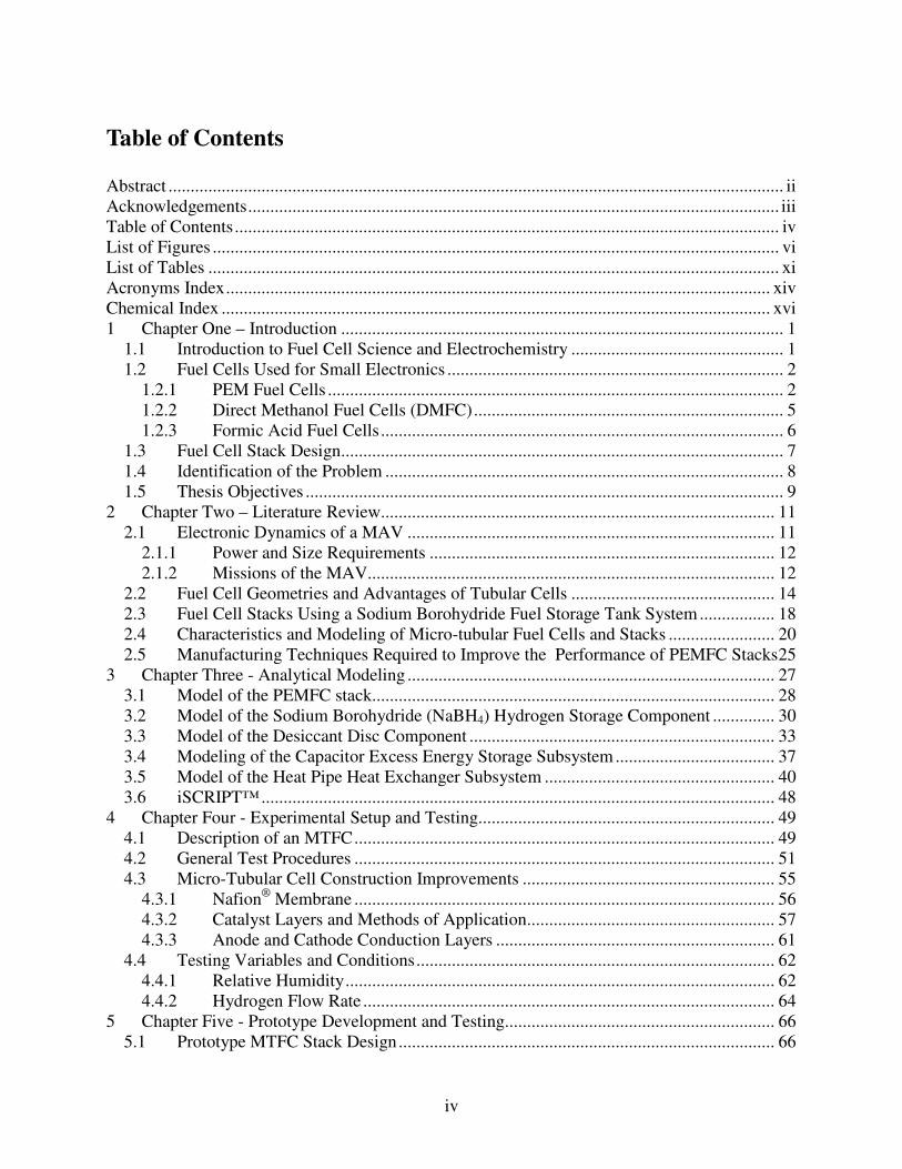
Figure 1.4. Direct methanol fuel cell diagram (DTI Energy, 2004; fair use). ............................... 6

Figure 1.5. A tubular fuel cell ready for insertion into a stack. ..................................................... 7

Figure 1.6. Diagram of four tubular fuel cells (the green circles) with the appropriate spacing, D,

between the cells to allow for airflow............................................................................................. 8

Figure 2.1. The Dragonfly MAV created by the University of Arizona (Paparazzi, 2006; fair

use). ............................................................................................................................................... 13

Figure 2.2. The mission flight trajectory for the University of Arizona’s Dragonfly MAV with

take-off, loitering, and landing (Mueller et al., 2007; used with permission of Dr. S.V.

Shkarayev). ................................................................................................................................... 13

Figure 2.3. The Casper 200/250 backpack-able UAV designed by the Israeli defense forces

(Defense Update, 2006; used with permission by N. Shental). .................................................... 14

Figure 2.4. Planar geometry for a fuel cell (Coursange, Hourri, and Hamelin, 2003; used with

permission of Dr. J. Hamelin)....................................................................................................... 16

Figure 2.5. Tubuar geometry for a fuel cell (Coursange, Hourri, and Hamelin, 2003; used with

permission of Dr. J. Hamelin)....................................................................................................... 17

Figure 2.6. Graphical comparisons between different chemical hydride storage systems,

hydrogen storage........................................................................................................................... 19

Figure 2.7. Polarization curve created from the mathematical modeling of planar and tubular

fuel cells (Coursange, Hourri, and Hamelin, 2003; used with permission of Dr. J. Hamelin). .... 24

Figure 2.8. Current density distribution. The lower curve represents planar fuel cell while the

upper curve represents the tubular fuel cell (Coursange, Hourri, and Hamelin, 2003; used with

permission of Dr. J. Hamelin)....................................................................................................... 24

vii

Figure 2.9. Polarization and power density results from testing of a PEMFC manufactured using

the techniques created by Eshraghi et al. (2005). ......................................................................... 26

Figure 3.1. Schematic of the power supply system with its subcomponents and energy and mass

flows.............................................................................................................................................. 28

Figure 3.2. Three-dimensional depiction of the NaBH4 hydrogen storage and delivery tank. .... 33

Figure 3.3. Trulite® NaBH4 tank fitting within the specified MAV fuselage parameters. The

electrical chip in front of the tank is a flow controller.................................................................. 33

Figure 3.4. The rate of absorption as a function of the relative humidity of the gas surrounding

the desiccant (Dick and Woynicki, 2002; reproduced with the permission of R. Park)............... 35

Figure 3.5. Schematic diagram of a heat pipe heat exchanger displaying the thermal cycle of the

device from the heat source to sink (Chemical Engineers’ Resource, 2008; used with permission

of S. Narayanan KR)..................................................................................................................... 41

Figure 4.1. A tubular PEMFC (i.e., MTFC) fabricated in 2007 during the previous phase with

mechanical parts labeled. .............................................................................................................. 49

Figure 4.2. MTFC schematic after fabrication............................................................................. 50

Figure 4.3. Cross sectional schematic of a MTFC....................................................................... 51

Figure 4.4. Fuel cell test station with supply lines labeled. .......................................................... 52

Figure 4.5. A MTFC (PEMFC) with gas flow inlet and outlets labeled...................................... 52

Figure 4.6. An MTFC attached to the fuel cell test station. This cell has been placed in a

humidity chamber. ........................................................................................................................ 53

Figure 4.7. The Solartron® Model 1480 8-channel potentiostat and its connection to the MTFC.

....................................................................................................................................................... 54

Figure 4.8. The chamber with a MTFC connected to the fuel cell test stand. ............................. 55

Figure 4.9. A tube of TT-060 Nafion® after being heated in deionized water............................. 56

Figure 4.10. A schematic of the catalyst layer/electrolytic membrane interface of the fuel cell.

The TPBs are shown in this figure and clearly represent the point at which all three phases meet.

....................................................................................................................................................... 59

Figure 4.11. A SEM image at 1000 �m scale of the cathode catalyst layer of a MTFC (FCF# 85)

fabricated by Luna Innovations, Inc. and tested at Virginia Tech. ............................................... 60

Figure 4.12. Photo of two of the materials used for the conduction layers: gold wire, and

Thornel® carbon fiber. .................................................................................................................. 61

viii

Figure 4.13. Planar Nafion® PEMFC polarization curves for different RHs and hydrogen and air

at standard temperature and pressure and 120° C (Zhang et al, 2008; used with permission of

Elsevier). ....................................................................................................................................... 63

Figure 4.14. Membrane conductivity (expressed as �) versus RH for a single cell operating at

120° C made with a Nafion® TT-112 membrane (Zhang et al., 2008; used with permission of

Elsevier). ....................................................................................................................................... 63

Figure 4.15. The Vaisala HUMICAP® humidity and temperature transmitter HMT337 (Vaisala,

2009; photo courtesy of Vaisala Inc.). .......................................................................................... 64

Figure 5.1. The prototype structure disassembled and labeled. ................................................... 67

Figure 5.2. Inventor™ drawing of a separation disc used in the prototype................................. 68

Figure 5.3. Inventor™ drawing of the large Teflon® sealing disc............................................... 69

Figure 5.4. Inventor™ drawing of the small Teflon® disc for the hydrogen delivery needles.... 70

Figure 5.5. Inventor™ drawing of the silicone septum placed inside the entering hydrogen gas

enclosure. ...................................................................................................................................... 70

Figure 5.6. Schematic illustrating the separation distances between MTFCs in the prototype

stack. ............................................................................................................................................. 71

Figure 5.7. The electrical PC board shown in the prototype structure. ....................................... 71

Figure 5.8. Electrical circuit of the printed circuit board placed in the prototype structure. ....... 72

Figure 5.9. Drawing of the prototype and forty tubular fuel cells in the stack. ........................... 73

Figure 5.10. Labeled design of the fuel cell stack prototype disassembled................................. 73

Figure 5.11. The prototype with six MTFCs installed and connected to the PC board on the left

side of the device. ......................................................................................................................... 74

Figure 5.12. An MAV with individual fuel cells placed in a “wingbone” like arrangement. ..... 74

Figure 5.13. Schematic of the prototype structure attached to the test stand ready for

experimentation............................................................................................................................. 76

Figure 5.14. Schematic of a prototype testing setup testing 12 MTFCs in series. ...................... 76

Figure 6.1. RH study of hydrogen gas leaving the Trulite® NaBH4 hydrogen storage tank. ....... 80

Figure 6.2. Graph of the amount of various desiccants needed to reach a specified RH. ........... 80

Figure 6.3. Cost required of each desiccant to reach a desired RH. ............................................ 81

Figure 6.4. Figure of merit for common working fluids over a broad temperature range

(Peterson, 1994; used with permission by John Wiley & Sons, Inc.)........................................... 84

ix

Figure 6.5. SolidWorks™ model presenting a schematic of the Dragonfly MAV (Mueller et al.,

2007; used with permission of Dr. S.V. Shkarayev)..................................................................... 85

Figure 6.6. Temperature profile of the water-copper heat pipe along its length. ........................ 88

Figure 6.7. Illustration of the number of Nafion® TT-060 prototype length MTFCs required for

the stack at varying temperatures to achieve a 24 W power output for the MAV........................ 90

Figure 6.8. Polarization curves calculated for various air RHs. .................................................. 91

Figure 6.9. Modeled polarization curve for MTFC with TT-050 and TT-060 type Nafion®. ..... 94

Figure 6.10. Open circuit voltage test results over a 12-minute time span................................ 103

Figure 6.11. Lifetime test of the first trial of the MTFC prototype. .......................................... 103

Figure 6.12. Second trial of the MTFC stack prototype lifetime test with 8 MTFCs................ 104

Figure 6.13. Lifetime test of the MTFC stack prototype with 12 MTFCs in the stack. ............ 104

Figure 6.14. First potentiodynamic (polarization) test of the 8-cell MTFC stack prototype..... 105

Figure 6.15. Second potentiodynamic (polarization) test of the 8-cell MTFC stack prototype. 106

Figure 6.16. Potentiodynamic test of the 12-cell MTFC stackprototype................................... 106

Figure 6.17. Second EIS of the 8-cell MTFC stack prototype................................................... 107

Figure 6.18. Electrochemical impedance spectroscopy of the 12-cell MTFC stack prototype. 107

Figure 6.19. Lifetime test of the MTFC stack prototype with 12 MTFCs in the stack dead-ended.

..................................................................................................................................................... 109

Figure 6.20. Polarization test of the MTFC stack prototype with 12 dead-ended MTFCs in the

stack. ........................................................................................................................................... 109

Figure 6.21. Electrochemical impedance spectroscopy of the MTFC stack prototype with 12

dead-ended MTFCs and a cathode relative humidity of 54%..................................................... 110

Figure 6.22. Electrochemical impedance spectroscopy of the MTFC stack prototype with 8

dead-ended MTFCs in 75% RH cathode environment. .............................................................. 111

Figure 6.23. Chemical schematic of Nafion® copper ion contamination in the MTFC membrane.

..................................................................................................................................................... 113

Figure C.1. Polarization test curve of VT 11, the best performing MTFC ever made throughout

the research. ................................................................................................................................ 128

Figure C.2. Lifetime test of VT 11, the best fabricated cell, over a 30 minute period. ............. 128

Figure C.3. Electrochemical impedance spectroscopy of VT 11 showing three distinct

impedance loss regions ............................................................................................................... 129

x

Figure C.4. Polarization curve of the best MTFC prepared by Luna Innovations and is a

modification of FCF 105 by testing it in a 100% RH air environment....................................... 130

Figure C.5. Electrochemical impedance spectroscopy of FCF 105-A, the best MTFC prepared

by Luna Innovations ................................................................................................................... 130

Figure C.6. Polarization curve of FCF 107-A, the second best performing Luna prepared fuel

cell, placed in air at an RH of 100% ........................................................................................... 131

Figure C.7. Electrochemical impedance spectroscopy (EIS) of FCF 107-A in 100% RH air... 131

xi

List of Tables Table 1.1. Comparison between the advantages and disadvantages presented when using

DMFCs............................................................................................................................................ 6

Table 2.1. Evaluation of various batteries used for electronic devices (Lund Instrument

Enginering, 2006; reproduced with permission of M.W. Lund)................................................... 18

Table 2.2. Comparison of different Nafion® membrane thicknesses using 2.0 M methanol. ..... 22

Table 2.3. Comparison of different Nafion® membrane thicknesses using 4.0 M methanol. ..... 22

Table 3.1. Model equations used to find the cell active surface area, power, and the number of

cells required in the stack.............................................................................................................. 29

Table 3.2. The variables and equations used in the NaBH4 subsystem model. ........................... 31

Table 3.3. Cost of each type of desiccant. ................................................................................... 34

Table 3.4. Equations for absorption capacity of desiccants......................................................... 35

Table 3.5. Additional model equations used for the desiccant disc component. ......................... 36

Table 3.6. Model equations used to find the surge time required by the MAV........................... 38

Table 3.7. Power surge times for various climb angles and rates................................................ 38

Table 3.8. Model equations used to determine the properties of the capacitor subsystem in the

MAV. ............................................................................................................................................ 39

Table 3.9. Governing equations for the heat transfer occurring through the heat pipe. .............. 42

Table 3.10. Table of working fluids for heat pipes, their properties, and useful range for

operation (Chemical Engineers’ Resource, 2008; used with permission of S. Narayanan KR)... 43

Table 3.11. Table of thermal conductivities and compatibility of various materials with working

fluids (Peterson, 1994). ................................................................................................................. 44

Table 3.12. Model assumptions and design options for the heat pipe model. ............................. 44

Table 3.13. Equation used to calculate the figure of merit for a working fluid........................... 45

Table 3.14. Model equations for the limitations of a heat pipe heat exchanger (Peterson, 1994).

....................................................................................................................................................... 46

Table 4.1. The Nafion® membrane tubing specifications for different model numbers (Perma

Pure, 2009). ................................................................................................................................... 56

Table 4.2. Varying hydrogen flow rates and the hydrogen mass supplied per hour for each...... 65

Table 6.1. Results of the NaBH4hydrogen storage tank iSCRIPT™ model................................ 78

xii

Table 6.2. Results of the iSCRIPT™ model for the capacitor energy storage component. ........ 82

Table 6.3. The size of the capacitor component for various climb angles and rates. .................. 82

Table 6.4. Modeled heat pipe entering and exiting temperatures for various working fluids and

building materials.......................................................................................................................... 86

Table 6.5. Values for the heat transport limitations of the heat pipe model and the heat

transferred across the device. ........................................................................................................ 88

Table 6.6. Description of operational changes made to run the best performing MTFCs........... 92

Table 6.7. Performance values for the four best fuel cells made during this research, including

data attained when they were modified. ....................................................................................... 92

Table 6.8. Average performance values for the Luna fuel cells fabricated with different Nafion®

types. ............................................................................................................................................. 94

Table 6.9. Performance values for Luna made fuel cells incorporating E-fill in the catalyst layer.

....................................................................................................................................................... 95

Table 6.10. PyVGCF study results. ............................................................................................. 96

Table 6.11. Results from the platinum study with various platinum loadings. ........................... 96

Table 6.12. Results of the sonication study on four Luna prepared fuel cells. ............................ 96

Table 6.13. Temperature study results for MTFCs processed at 150° C, 170° C, and 200°C. ... 97

Table 6.14. Catalyst ink blow out study results. .......................................................................... 98

Table 6.15. Needle type study results. ......................................................................................... 99

Table 6.16. Cathode collection layer study results. ..................................................................... 99

Table 6.17. Performance values for the MTFCs intended for the prototype (PR cells). ........... 100

Table 6.18. MTFCs used in three prototype structure setups for testing. .................................. 101

Table 6.19. Prototype cell orientation test results...................................................................... 101

Table 6.20. Prototype cells modification study results. ............................................................. 102

Table 6.21. Operating conditions for the prototype tests ran..................................................... 108

Table A.1. Variations in MTFC characteristics which were tested throughout the project....... 124

Table B.1. Model results for the amount of desiccant needed to adjust the hydrogen gas flow to

specific RHs. ............................................................................................................................... 126

Table B.2. Model results of the fuel cell stack presenting the quantity of cells required for the

MAV. The cell active area is that for the PR MTFCs. .............................................................. 126

xiii

Table B.3. Electrical characteristics of Maxwell Boostcap® ultracapacitors used for the MAV

model (Maxwell® Technologies, 2009). ..................................................................................... 127

Table D.1. Bill of materials for the fuel cell prototype.............................................................. 132

Table D.2. Procedure to prepare a Nafion® membrane in TBA in methanol............................. 132

xiv

Acronyms Index BATMAV Battlefield air trajectory

micro-air vehicle BOP Balance of plant CESR Center for Energy Systems

Research CFD Computational fluid

dynamics CNF Carbon nano-fiber DI Deionized DMFC Direct methanol fuel cell E0 Standard reduction potential EIS Electrochemical impedance

spectroscopy

ENV Emission neutral vehicle FAFC Formic acid fuel cell FCF Fuel cell fiber GDL Gas diffusion layer HOD™ Hydrogen on Demand™

ICTAS Institute for Critical Technology and Applied Science

ITAR International Traffic in Arms

Regulations

IUPAC International Union of Pure and Applied Chemistry

M Molar

MAV Micro-air vehicle MeOH Methanol MEA Membrane electrode

assembly MTFC Micro-tubular fuel cell OCV Open circuit voltage PC Printed circuit PEM Proton exchange membrane PEMFC Proton exchange membrane

fuel cell

PFSA Perflourosulfonic acid PTFE Polytetraflouroethylene

(Teflon™) PR Prototype PR(X;Y. . ) Modified Prototype PyVGCF Pyrograph vapor grown

carbon fiber RH Relative humidity SCCM Standard cubic centimeters

per minute

SEM Scanning electron microscope

STP Standard temperature &

pressure

TBA Tetra-butyl ammonium

xv

TPB Triple phase boundaries UAV Unmanned aerial vehicle

USAF United States Air Force

VT Virginia Tech

xvi

Chemical Index Ar Argon CH4 Methane CH2OH Methanol CO Carbon monoxide CO2 Carbon dioxide Cu2+ Copper ion H2 Hydrogen gas H+ Proton H2CO2 Formic Acid H2O Water H2O2 Hydrogen peroxide H2SO4 Sulfuric Acid N2 Nitrogen gas NaBH4 Sodium borohydride NaBO2 Sodium borate NaOH Sodium hydroxide O2 Oxygen Pt Platinum Ru Ruthenium

1

1 Chapter One – Introduction As societies around the world develop their defense sectors, the need for small

reconnaissance electronics and advanced technology greatens. These small electronic devices

require high power densities and more energy than has been needed in the past. Rechargeable

batteries, the current energy source for these devices, provide only limited power that does not

sufficiently meet energy needs. To accommodate advanced power requirements and quicker

recharge times, an alternative power source is needed.

One alternative energy source which has been heavily investigated is the fuel cell system.

Fuel cells are power source devices which have high energy densities, are environmentally clean

(at least locally), and have a quick fuel recharge time. These qualities make them perfect

candidates as an alternative power source in small advanced electronics and available alternative

to the current rechargeable battery.

1.1 Introduction to Fuel Cell Science and Electrochemistry Fuel cells are devices which can provide energy to electronics, motorized vehicles, etc.

These devices are a form of direct conversion energy which utilize electrochemical instead of

chemical reactions to produce electricity. This is accomplished by “capturing” and directing

electrons produced by electrochemical reactions through the use of impermeable membranes and

conduction layers. In an ideal and unrealistic world, a single cell will produce the same voltage

output as the standard reduction potentials (denoted Eo in the literature) associated with the

utilized electrochemical equations. Fuel cells never operate at these reduction potential levels

due to various associated losses. These associated losses result in lower efficiencies for the cell,

which researchers worldwide are trying to optimize. Despite their presently lower efficiencies,

fuel cells show promising power and current outputs when placed in stacks, which are

comparable to their more commonly used energy producing competitors. Additionally, fuel cells

are considered an ideal energy source because they are easily fuel rechargeable, have generally

smaller damaging effects on the environment.

2

Fuel cell technology has been in existence since before the Civil War. However, fuel cell

implementation in electronics and transportation has only been explored recently because of the

rising cost of oil and a desire for corporations to become “green.” In fact, in 2005, the first

motorcycle operated by fuel cells was produced by Intelligent Energy, a British technology firm

specializing in fuel cell production and clean energy sources. The vehicle, called the Emission

Neutral Vehicle (ENV), can travel for 100 miles before refueling (Arellano, 2006).

Fuel cells are energy factories, like the combustion engine, which oxidize the fuel with

oxygen to produce power and water. In common practice, the fuel of choice is hydrogen gas

(H2). Methane (CH4), carbon monoxide (CO), and methanol (CH2OH) have also been used as

fuels to power fuel cells. Extensive research at the university level focuses on proton exchange

membrane fuel cells (PEMFCs) and direct methanol fuel cells (DMFCs) and the advantages of

using them in electronics and for transportation. Fuel cells, unlike lithium-ion or conventional

batteries, are easily rechargeable because the only recharge requirement is refilling the fuel tank.

As long as fuel is provided to the fuel cell it will continue to operate.

1.2 Fuel Cells Used for Small Electronics

1.2.1 PEM Fuel Cells

Of the many fuel cell variations, PEMFCs have proven to be the most suitable for

transportation and portable electronic devices. PEM fuel cells are considered suitable for

transportation because they operate at lower temperatures between 50° C and 80° C and are often

made from Nafion®, a readily available electrolytic membrane formulated by DuPont®. These

membranes allow for protons to be transferred while simultaneously preventing negatively

charged electrons, fuel, or oxygen gas from passing through them. Nafion® allows protons to

pass because of the presence of sulfonic acid group sites. The proton bonds to the negative site,

then “hops” to the next polymer molecule, continuing this process until it reaches the opposite

side of the Nafion® membrane. The IUPAC chemical structure of Nafion®, with the sulfonic

acid group circled is presented in the Figure 1.1.

If the fuel supply permeates through the membrane, it is referred to as fuel or gas

crossover. Fuel crossover, whether due to a puncture or dehydration of the membrane, is one of

3

the primary causes for power loss and damage to a fuel cell. Research has been done in this area,

and great strides are being taken to reduce fuel crossover and make better PEMFCs.

Figure 1.1. The Nafion® molecule found in the membrane. The circled section represents the sulfonic acid group which makes this organic chain unique from PTFE Teflon®.

Fuel flows parallel to the anode and runs through a channel to the PEMFC, as depicted in

Figure 1.2. The anode, the negative terminal electrode of the PEMFC, is the site at which

hydrogen gas reacts with an applied catalyst ink to create a positively charged proton and an

electron. The electrochemical equation for this half-reaction and its associated oxidation

potential are (Brown et al, 2003):

H2 �2H+ + 2e- Eo(v)=0.00 (1.1)

Figure 1.2. Diagram of a PEMFC (EcoGeneration Solutions, 2002; used with permission of EcoGeneration

Solutions, LLC).

4

This is often referred to as splitting of the molecule, which, by itself produces no electrical

voltage potential. Platinum is commonly used in industry as a catalyst for fuel cell applications

and is mixed with Nafion® solution, carbon powder or ruthenium, and glycerol to create an ink,

which is then painted on the electrodes. From this point, protons (H+) flow through the Nafion®

membrane, while electrons, which cannot pass through the membrane, flow through an electrode

collector, typically a plate or conducting wire.

The electrons travel through the conducting wire or plate and provide power to an

external capacitor, motor, printed circuit board, etc. The electrons then travel to the cathode on

the opposite side of the membrane. The cathode is connected to a flow channel which supplies

oxygen (air) gas; and at this interface, protons, electrons, and oxygen (O2) unite to form pure

water. The electrochemical equation representing this half-reaction occurring on the cathode

side of the fuel cell and its reduction potential is given by (Brown et al, 2003):

4H+ + 4e- +O2� 2H2O Eo(v)=1.23 (1.2)

Water is the only natural byproduct of hydrogen fed PEMFCs, making this source of

energy locally environmentally safe1. Figure 1.3 shows a PEMFC within a testing apparatus.

Figure 1.3. A PEMFC in a testing apparatus (U.S. Department of Energy, 2008; public domain).

1 Since H2 is not a naturally occurring fuel, it must be produced via reformation or electrolysis. In both cases emissions occur in the process (the former) or upstream of the process (the latter) depending, of course, on how the electricity in the latter is produced.

5

An ideal, single membrane PEMFC should produce a starting open circuit voltage (OCV)

of Eo before any activation, ohmic, and concentration losses occur (O’Hayre et al., 2006). To

optimize the power output of the PEMFC, fuel crossover must be eliminated, catalyst must be

applied uniformly, and the membrane must be sufficiently hydrated.

1.2.2 Direct Methanol Fuel Cells (DMFC)

Another type of fuel cell that is ideal for portable electronic devices is the direct methanol

fuel cell (DMFC). DMFCs are proton exchange membrane fuel cells that use methanol

(CH3OH) as the fuel, not hydrogen. Methanol is a toxic and flammable organic chemical that is

cheap, readily available, and mass produced. Since it is a liquid at room temperature and

pressure, it is also easier to store than hydrogen gas as no pressurization is required for storage

and no conversion is required using a chemical or metal hydride.

Figure 1.4 depicts a DMFC and the chemical reactions that occur within the cell. As

shown in the diagram, a DMFC is simply a PEM fuel cell that utilizes methanol. The primary

differences between a DMFC and hydrogen PEMFC is the number of electrons that pass through

the appended load and the chemical byproduct.

In the DMFC, a methanol/water mixture is supplied to the anode, which is painted with a

platinum-ruthenium based catalyst, to produce H+ protons and carbon dioxide (CO2) gas as a

byproduct. Some unused water and methanol remains after the reaction, but are typically

recycled back into the anode fuel delivery channel. As was seen in the PEMFC, Nafion® is the

membrane used to prevent the passage of electrons and allow the permeation of H+ protons.

Using methanol fuel for a DMFC has clear advantages in ease of use and safety. As stated

earlier, methanol is stored as a liquid not under pressure. Therefore, military personnel who

carry a vehicle powered by a DMFC do not face the risk of a possible explosion due to sudden

pressure loss or physical punctures in the fuel tank. However, DMFCs and methanol also have

clear disadvantages. A list of advantages and disadvantages for DMFCs is given in Table 1.1.

As can be seen in the table, the advantages of DMFCs are that the methanol has a higher

density than hydrogen, the aqueous fuel increases the lifespan of the DMFC Nafion® membrane,

and methanol storage is easier and safer than alternative fuels (O’Hayre et al., 2006). The

disadvantages, however, are that direct methanol fuel cells have lower efficiencies, operate at a

low cell voltage and current density, and contain volatile fuel.

6

Figure 1.4. Direct methanol fuel cell diagram (DTI Energy, 2004; fair use).

Table 1.1. Comparison between the advantages and disadvantages presented when using DMFCs.

Advantages Disadvantages

Liquid fuel allows for easy storage and

handling.

Has a higher energy density than H2.

Humidification of the reactant is not

necessary.

Aqueous fuel allows the membrane to last

longer due to polymer hydration.

DMFC fuel efficiency is lower, less than

25%.

Operates at a low cell voltage and current

density.

Carbon dioxide (CO2), a greenhouse gas, is a

byproduct of the cell.

Methanol is toxic and volatile, and may cause

blindness if ingested.

1.2.3 Formic Acid Fuel Cells

Formic acid (HCOOH, or H2CO2) is a non-reformed liquid which may also be used as a

fuel supply fed directly to the cells. This alternative fuel to hydrogen is an intermediary

chemical created during the oxidation of methanol to release electrons.

Formic acid fuel cells (FAFCs) have already been used in the production of laptops and

small electronic devices. Formic acid, like methanol and hydrogen, has both advantages and

disadvantages. When formic acid is used, fuel crossover is not a significant problem in the

membrane layer. Therefore, a higher concentration of formic acid fuel supplied on the anode

side does not create performance problems and may provide more power than methanol even at

lower heating values. Additionally, formic acid is not as toxic as methanol. However, little is

known about the concentration threshold of this fuel fed to the anode before catalyst poisoning

occurs and affects the cell’s performance (Gunter, 2007).

7

1.3 Fuel Cell Stack Design

Due to high energy requirements, one fuel cell, even operating with an OCV of 1.23 v

does not provide enough power to operate today’s small electronic devices completely.

Therefore, stacks incorporating many fuel cells are required. For this to be created, a design

must be made for the stack that accounts for fuel dispersion, cell orientation, and volume

requirements within the device. Additionally, for DMFCs, ventilation holes are necessary so that

carbon dioxide (CO2) can escape. A design which allows the fuel cell stack to perform optimally

regardless of its orientation and with ease of construction is vital for creating a reliable power

source. A governing factor in determining how to design this stack is the geometry of the fuel

cell, which may be either, for example, planar or tubular. Figure 1.5 shows an example of a

tubular fuel cell, which is particularly useful for applications with limited space and non-cubical

geometries. When placed in a stack, there are small spaces separating individual tubular cells,

which allow oxygen to passively flow through the stack. Cell spacing is important because

without a supply of oxygen to the cathode, protons cannot be oxidized and produce water, and as

a result the stack will suffer a large power loss. Ideally, the spacing between individual cells

should be 0.51 mm to allow proper air flow through the stack, as shown in the diagram of Figure

1.6. This spacing was calculated by Kimble et al. (2000) who utilized a computational fluid

dynamics (CFD) flow solver called Compact 2-D, version 2.0, to calculate that effective spacing

required for air to circulate through a tubular fuel cell arrangement.

Figure 1.5. A tubular fuel cell ready for insertion into a stack.

8

Figure 1.6. Diagram of four tubular fuel cells (the green circles) with the appropriate spacing, D, between the cells

to allow for airflow.

Another important factor to be considered when designing a planar or tubular fuel cell stack

is the quantity of cells needed to reach the device’s power requirements. Quantity plays an

important role in creating a configuration of tubular fuel cells, especially if the dimensions

allotted for the cell stack are limited. Determining how many fuel cells are required is based on

the power requirement for the electronic device and the power output of the individual cell. The

power output is found by running various tests such as a potentiostatic, potentiodynamic, and

electrochemical impedance spectroscopy tests. The voltage requirement also plays a factor in

fuel cell quantity as a desired voltage to operate a vehicle must be met. Determination of cell

quantity in a stack in this fashion applies to both planar and tubular geometries.

1.4 Identification of the Problem In an effort to improve the power plant for a micro-aerial vehicle (MAV), the U.S. Air

Force is now investigating alternative energy sources to power these devices. Currently,

rechargeable batteries are being used as the MAV power plant, and until recently, have been

quite effective. However, as these devices become more vital for homeland security and

warfare, they require more advanced technology and higher power inputs and densities.

Unfortunately, with the current battery technology, rechargeable and non-rechargeable batteries

fall short of these modified MAV power requirements. The only way to potentially improve

battery power output is by increasing their volume and mass, and unfortunately, the stringent

space and payload requirements of this small vehicle cannot accommodate a size increase. In

addition, the defense forces would like to increase typical mission durations of the MAV, and

D= 0.51 mm

Flow of air

9

cannot do so given that batteries are unable to endure long time periods without required

recharge.

To accommodate the size, time, and power requirements of a MAV, energy sources

different than batteries must be implemented. One solution is a micro-fuel cell system, which is

capable of reaching higher power outputs and energy densities than conventional batteries and is

small enough to fit inside a clandestine device. Even at low efficiencies, micro-fuel cell systems

can produce a higher power output and/or have a higher energy density than rechargeable and

non-rechargeable batteries. Also, the micro-fuel cell system does not require frequent and

lengthy recharges, like its battery counterpart. The micro-fuel cell system, its cell geometry,

fabrication, and size are investigated in this thesis research.

1.5 Thesis Objectives

The aim of this thesis research is to develop a prototype micro-tubular fuel cell system

for use in a MAV. This will require computer modeling, construction of the design, and testing

of micro-tubular fuel cells and a stack prototype which can provide sufficient power to a MAV.

The lumped-parameter (or 0D) modeling will address components of the power supply system

only partially tested such as the hydrogen gas storage unit in hopes of optimizing gas output

while minimizing its occupying space. It is believed that this can be done using some type of

chemical hydride tank. The modeling will also address components of the system not tested such

as an energy storage unit which will provide additional power during maximum transient current

draws, which occurs when the vehicle is ascending or descending. The envisioned solution here

is a capacitors or set of capacitors.

Numerical modeling will be performed using iSCRIPT™, a mathematical analysis

program created by TTC technologies. Using the programming language of iSCRIPT™ and the

Crimson Editor programming text editor, models will be created of the fuel cell system and its

associated components. The model will also determine if implementation of the system within

an MAV is feasible or if design alterations must be made to the aircraft.

To accomplish both the hardware and modeling aspects of this thesis research, the

following objectives will be addressed:

10

• Provide a general overview of planar and tubular fuel cells, their fundamental

science, and electrochemistry.

• Define the power requirements and mission for a reconnaissance based MAV.

• Develop a procedure for manufacturing micro-tubular fuel cells (MTFCs) by

creating a cell of a specific length, conductor material, catalyst layers, and other

characteristics that will produce optimum performance based on experimentation.

• Model a capacitor-based energy storage unit for use when the MAV demands

high power levels during takeoff and landing.

• Model, with iSCRIPT™, a desiccant disc which regulates the hydrogen or fuel

gas relative humidity being supplied to the fuel cell stack as well as a hydrogen

gas storage tank utilizing a chemical hydride.

• Model a heat pipe using iSCRIPT™, to recover energy from a high temperature

section of the aircraft and transfer it to the fuel cell stack in order to increase its

operating temperature.

• Discuss a MTFC stack prototype, its design characteristics, results from testing it,

and provide recommendations for future implementation

11

2 Chapter Two – Literature Review

Extensive research has been conducted on MAVs as well as tubular PEMFCs and

DMFCs, which is relevant to the work presented in this thesis. This chapter provides a brief

overview of the literature, which pertains to the application (the MAV) and its possible mission

trajectory, numerical modeling of the energy system, and the fuel cell fabrication for the stack

prototype envisioned. This chapter will also explain why tubular fuel cells are more desirable

than either planar fuel cells or conventional batteries in small electronic devices like the MAV.

The literature reviewed is presented in four sections:

• The electronic dynamics of MAVs.

• Advantages of tubular fuel cells over planar PEMFCs and common batteries.

• Fuel sources for the fuel cell system and their storage methods.

• Fuel cell fabrication techniques and materials and their impact on performance.

These four topics are the basis for the research, modeling, and experimentation conducted for

this thesis.

2.1 Electronic Dynamics of a MAV

In order to place a stack of fuel cells in an MAV to serve as a power source, certain

information regarding the vehicle must be known. These include a full understanding of the

power requirements and flight mission specifications (or trajectory). This information will

specify exactly how much power is needed from the fuel cell stack, the duration of the fuel cell

stack’s operation for a single mission, and the quantity of fuel cells required for the stack to

power the mission. A complete understanding of MAV energy requirements and a detailed

description of a mission is needed before a power system can be modeled, and a PEMFC stack

can be built and placed inside the MAV.

12

2.1.1 Power and Size Requirements

Since the MAV is to be used by the United States Air Force, strict power and size

requirements are those dictated by the Air Force Solicitation F061-144-0607 (Topic # AF06-

144). In it, the Air Force states that the MAV must have a minimum current draw of at least 2 A

and 12 v for the fuel cell stack (totaling 24 W of power). The size of the fuel tank by volume

should preferably not exceed 10.16 cm × 1.59 cm × 3.18 cm (4 in × 0.625 in × 1.25 in), totaling a

volume of 0.051 L (51 cm3). This volume has traditionally been occupied by a rechargeable

battery supplying power to the MAV. This space, however, could also be occupied by the fuel

cell stack, or any component of the MAV power plant system.

2.1.2 Missions of the MAV

In addition to the power requirements, a mission of the MAV must also be specified in

order to quantify the operating period required of the fuel cell stack by the MAV. The mission

will also indicate how much time is required of additional energy storage devices, which provide

additional power during power surge periods. The mission for the MAV consists of three

segments; launch, cruise (also called loitering), and landing. The launch and landing segments

may also be called surge periods because additional power over and above what can be provided

by the fuel cell is needed for the MAV. It is because of these two surge periods that an energy

storage subsystem of capacitors will be needed as part of the fuel cell system to provide

additional power to the MAV.

The University of Arizona’s MAV project has designed a vehicle called the Dragonfly,

which spans approximately 12 in (30 cm) and has high maneuverability. The Dragonfly (shown

in Figure 2.1) is an award-winning MAV, taking first place at the U.S.-European Micro-Aerial

Vehicle Technology Demonstration and Assessment in 2005 (Mueller et al., 2007).

The Dragonfly is very similar to the MAV which will be used for the fuel cell stack

implementation here since it is equipped with a rechargeable battery, global positioning system,

video camera, and a remote control (RC) receiver. The Dragonfly is given a flight mission

trajectory lasting 30 min, and reaches an altitude of 60 m (197 ft). To accommodate for the high

wind gusts, the plane climbs during launch at low angles, 6 or 18 degrees, and at velocities of 2

m/s (4 mi/hr) to 6 m/s (13 mi/hr). During the cruise portion of the mission, the Dragonfly can

13

achieve speeds of approximately 22 m/s (49 mi/hr). The average cruise speed for the Dragonfly,

however, is around 12 m/s (27 mi/hr). For this mission trajectory, the MAV does several figure

8s during the cruise portion before beginning its descent. During the landing segment of the

mission, the Dragonfly glides at an angle of about 14.06 degrees and a speed of 2 m/s (4 mi/hr).

Due to the soft angle of descent and low speed, the MAV requires a landing distance of roughly

120 m (394 ft) (Mueller et al, 2007). The Dragonfly’s mission and flight path is a very detailed

one and can, therefore, be easily used for numerical modeling. It is shown schematically in

Figure 2.2.

Figure 2.1. The Dragonfly MAV created by the University of Arizona (Paparazzi, 2006; fair use). There are many other missions for MAVs that differ in time, rate of climb or descent,

maximum altitude, and velocity. One example is the mission of a Casper 200/250, a back-

packable surveillance MAV, which was designed by Top I Vision to meet the UAV requirements

Figure 2.2. The mission flight trajectory for the University of Arizona’s Dragonfly MAV with take-off, loitering,

and landing (Mueller et al., 2007; used with permission of Dr. S.V. Shkarayev).

14

for the Israeli Defense Forces. It is a 1.3 m (51.18 in) long MAV which can maintain speeds of

21 to 80 km/hr (13-50 mi/hr).

This vehicle has a 7 m/s (15 mi/hr) rate of climb and can reach an altitude of 250 m

(820 ft). Like the Dragonfly, the Casper 200 also descends with a soft angle and a 1:15 glide

ratio. Additionally, the vehicle has a high handling and maneuvering capability (Defense

Update, 2006).

Another MAV mission trajectory is that given for a BATMAV, created by

Aerovironment, Inc. BATMAV stands for Battlefield Air Targeting Micro-Air Vehicle and is

used for surveillance purposes. This vehicle’s mission may reach altitudes up to 152 m (500 ft.)

and a cruising speed of 17.9 m/s (40 mi/hr). Other than these details, little is found in the

literature about full missions of the BATMAV or the Casper 200 because of their current use in

the armed forces. Because of this lack of detail, it is very difficult to model an energy source for

these missions. Thus, the Dragonfly mission will be used here for modeling a fuel cell stack

system (Defense Update, 2009).

Figure 2.3. The Casper 200/250 backpack-able UAV designed by the Israeli defense forces (Defense Update, 2006;

used with permission by N. Shental).

2.2 Fuel Cell Geometries and Advantages of Tubular Cells

Fuel cells, regardless of the fuel being supplied to it, are typically created in two major

geometries, planar and tubular. Currently, planar fuel cells serve as the dominant application due

to the ease of manufacturing a membrane electrode assembly (MEA) with this geometry and due

15

to the experience and extensive research literature available on this type of configuration.

However, for many applications, tubular fuel cells may be the best option. If size allotment for

the cell stack and active surface area of the electrodes are concerns for the energy system, then

perhaps a tubular fuel cell stack may be a more desirable candidate. Planar fuel cells may

require more space due to their “box-like” arrangement. Below is a brief list of the advantages

associated with using tubular fuel cells over their planar counterparts (Steyn, 1996):

• Tubular fuel cells do not suffer parasitic losses due to edge effects.

• Metal or serpentine flow fields are eliminated.

• There is a uniform pressure applied to the MEA by the cathode current collector

applied through a conduction layer.

• The cathode surface area is greater than that of the anode, which reduces the oxygen

reduction overpotential.

• Tubular cells have higher volumetric energy densities because they can achieve a

higher active area to volume ratio.

• Tubular geometries do not require the need for pumps, fans, or other devices (Al

Baghdadi, 2008).

Although there clearly appears to be advantages to tubular fuel cells, there are also

several disadvantages to this geometry as well, i.e,

• It is difficult and more time consuming to paint the anode and cathode sides of the

cell uniformly with catalyst ink.

• It is difficult to develop an MEA for the tubular cell due to its geometry and small

size.

• It is difficult to hot press these cells due to their tubular geometry; great care must be

taken in order to avoid pinching the membrane.

• There is not much literature available devoted to tubular fuel cell research.

The use and research of low-temperature (e.g.., PEM or DMFC) tubular fuel cells is relatively

unexplored, with only a handful of articles available on the subject matter. The literature that is

available, such as that by Coursange, Hourri, and Hamelin (2003), prove that higher power

densities are achievable with micro-tubular fuel cells over planar fuel cells because MTFCs have

16

lower activation potentials. Additionally, the literature has concluded that gas is more uniformly

distributed in a tubular geometry, resulting in better use of fuel in these types of cells. This is an

ideal situation for smaller confines where fuel must be stored alongside the cell stack. The little

literature that is available suggests that a micro-tubular fuel cell, with additional experimentation

and modification according to the space allotment and application, will create a higher

performing stack for small portable devices than a planar cell configuration. Thus, for an MAV,

which can only accommodate a fuel cell stack and system fitting within a small volume and

having a low mass, the MTFC geometric configuration appear to be the best option available.

The advantages and disadvantage of planar and tubular fuel cells can perhaps be better

perceived if displayed visually. Figure 2.4 presents the planar geometry with the gas flow

direction and Figure 2.5 presents the tubular cell geometry with flow direction.

Figure 2.4. Planar geometry for a fuel cell (Coursange, Hourri, and Hamelin, 2003; used with permission of Dr. J.

Hamelin). In figures 2.4 and 2.5, (a) and (f) represent the cathode and anode flow channels, (b) and (e)

represent the gas diffusion layers, (c) and (d) are the electrochemically active regions, and (g)

and (h) represent small perforated plates (at Virginia Tech, these represent the anode and cathode

collection layer).

In figure 2.4, the catalyst layers are represented by (c) and (d). The tubular geometry,

since it only requires hydrogen gas storage and no serpentine flow channels, is more space

efficient particularly for small portable devices.

Fuel cells, regardless of their geometry, tend to have higher power densities than

conventional batteries or newer battery types. The power density required of the fuel cell by the

Air Force MAV is 0.75 W-hr/cm3 (Gunter, 2007), which is higher than that available from most

17

Figure 2.5. Tubuar geometry for a fuel cell (Coursange, Hourri, and Hamelin, 2003; used with permission of Dr. J.

Hamelin). batteries with the exception of zinc-air, as can be seen from Table 2.1. Batteries have some other

disadvantages as well. For example nickel metal hydride and nickel cadmium batteries have a

high self discharge rate and do not produce a high voltage or power density. More than a dozen

Ni-Cad or Ni-MH batteries would be needed in a pack to provide sufficient power. Similarly

Thunder Power batteries are heavy, and have virtually no charge memory. This is not a desirable

trait for an MAV with mission times of an hour or greater. In addition, the Thunder Power

batteries have a volume that is too large to fit inside the MAV fuselage. As stated earlier, the

only battery in the evaluation which has a high power density is a zinc air battery, 1.637 W-

hr/cm3. In addition, zinc air batteries also have a low self discharge rate, an advantage for MAV

technology. However, these batteries are not rechargeable, which poses a great disadvantage if

an MAV must perform several flight missions over a short period of time (i.e, one day). It has

been shown that both tubular and planar fuel cells can achieve high power levels, because their

possible fuel sources, hydrogen and methanol, have theoretical power densities of 7 W-hr/cm3

(using hydrogen gas derived from metal hydrides), and 4 W-hr/cm3 (liquid methanol) (Larminie

and Dicks, 2003). If the fuel cells have a high efficiency, a power density near these values may

be achieved. Even at low efficiencies, the power density is higher than those for the batteries

displayed in Table 2.1. In addition, fuel cells are lightweight and have a finite charge memory

dependent on the amount of fuel being supplied to them.

With the requirement of 24 W power and a 0.75 W-hr/cm3 power density, a tubular

PEMFC stack would be the most ideal for this application due to its small size and ease of use.

18

Table 2.1. Evaluation of various batteries used for electronic devices (Lund Instrument Enginering, 2006; reproduced with permission of M.W. Lund).

Volume

(cm3) Weight

(kg) Voltage

(v) Capacity (mAhr) W-hr/cm3 W-hr/kg W hr

Li-ion Polymer 32.430 0.018 3.7 650 0.07 133.61 3.80 Thunder Power I-3SPL 68.000 0.142 11.1 2100 0.34 164.15 17.55 Thunder Power I-4SPL 88.400 0.178 14.8 2100 0.35 174.61 18.00

Ni-MH 4.390 0.015 1.2 330 0.09 26.40 4.62 Ni-Cad 4.181 0.011 1 280 0.07 25.45 3.43

Zinc Oxide 0.265 0.00083 1.4 310 1.64 522.89 83.87

Currently, Lithium-ion polymer batteries are used for the MAV, which, although they fit the

volume requirement of 51.209 cm3, provides much less power than specified by the Air Force.

With an efficient and small hydrogen fuel tank fitting within the battery’s current space and a

fuel cell stack providing a greater power density than that observed for a Lithium-ion polymer

battery, a power supply system for the MAV meeting all the requirements stated by the Air Force

may be possible.

2.3 Fuel Cell Stacks Using a Sodium Borohydride Fuel Storage Tank System

Hydrogen is often stored in a gaseous form when delivered as fuel for fuel cells in the

transportation industry. However, hydrogen gas must be stored under high pressure, making it

difficult for cells in small electronics or portable devices since high pressure tanks are heavy,

bulky, and may produce an explosion or personal injury. Safety and storage are important for the

MAV, which is why using a chemical hydride for hydrogen storage is better and safer. Chemical

hydrides provide hydrogen gas by converting it from a hydride, such as sodium borohydride

(NaBH4). Sodium borohydride is the preferred hydride system because it produces pure, humid

hydrogen gas under room temperature and pressure. It also involves an exothermic reaction for

hydrogen liberation, which means it requires no heat input to activate. The chemical equation

for the reaction of sodium borohydride with water to release hydrogen gas is:

NaBH4 + 2 H2O � 4H2 + NaBO2 (aq) + approximately 300 kJ (2.1)

19

Four molecules of hydrogen gas are produced, and the sodium borate byproduct can be

recycled into NaBH4. Sodium borohydride contains 10.6% hydrogen by weight and

theoretically, can produce an energy density of 9.3 W-hr/g. Although NaBH4 has a lower weight

percentage of hydrogen than lithium chemical hydrides, the byproduct sodium borate can be

easily recycled to produce NaBH4. The lithium hydrides can not be recycled back as easily from

the product of the water/lithium hydride reaction. In addition, literature about lithium chemical

hydrides is not as available because, on a per pound basis, they are much more expensive than

NaBH4, and therefore not as heavily researched. It is because of these reasons that NaBH4 is an

ideal chemical hydride2 storage system for small electronics and portable devices. Additionally,

this reaction is an exothermic one. Thus the energy dissipated from it can be harvested to

increase the temperature of the fuel cell stack, if needed.

Figure 2.6 compares the various storage systems with respect to the percent of hydrogen

by weight and the percentage of hydrogen in a stoichiometric mix with water (Wu, 2003).

02468

101214161820

LiBH4 LiH

NaBH4

LialH4

AlH3

MgH2

NaAlH4

CaH2NaH

wt

% H

sto

red

% H by weight% H in sto ichiometric m ix w/water

Figure 2.6. Graphical comparisons between different chemical hydride storage systems, hydrogen storage.

2 . Metal hydrides are sometimes classified as classical/interstitial, chemical, and complex, light-metal (Chandra, Reilly, and Chellapa, 2006). In this classification scheme, NaBH4 is a complex, light-metal hydride as are all the metal hydrides shown in Figure 2.6. A chemical hydride in this scheme is an organic compound such as methanol, methylcyclohexane, ammonia, ammonia borane, etc. which can be reformed to generate hydrogen. However, the term “chemical hydride” as employed in this thesis work (U.S. DOE, 2008) is any metal hydride that can be used in a chemical reaction to produce hydrogen. Thus, all the so-called “complex, light-metal hydrides” fall within this definition.

20

Millennium Cell (prior to bankruptcy in August 2008) has been working vigorously to

improve chemical hydride hydrogen storage systems since they have been shown to be a

promising method of hydrogen storage for fuel cells in small electronics and portable devices

(Wu, 2008). Trulite®, another firm which is currently focused on NaBH4 hydrogen storage

tanks, has successfully reproduced a tank system which can also produce humid pure hydrogen

gas and thermal energy. In addition, the tank fabricated by Trulite® containing sodium

borohydride fits inside the volume specified for the fuselage by the Air Force. The governing

principles and equations used by both Trulite® and Millennium Cell was used to produce an

iSCRIPT™ model of the hydrogen storage system.

2.4 Characteristics and Modeling of Micro-tubular Fuel Cells and Stacks

Based on the work of R. Evans (2008), which developed the basis for the work conducted

during the research presented in this thesis, it was assumed that eventually DM MTFCs would be

modeled, developed, and tested here once work on modeling, developing, and testing of

hydrogen MTFCs had been completed. However, due to time constraint and limited resources

this did not materialize even though DM MTFCs still hold promise for their eventual use in

MAVs. With this in mind, this section reviews the relevant work in the literature both in respect

to DMFCs and PEMFCs.

To begin with, recent investigations into the use of methanol as a fuel in PEMFCs has

been conducted at many research institutions because methanol has a high energy density (6100

Whr/kg at 25° C (Liu et al., 2006)), can be stored easier than hydrogen gas, and has a relatively

low cost. These desirable qualities make it an ideal fuel for powering laptops, small electronics,

and potentially MAVs. One major challenging issue of both active and passive DMFCs is the

presence of methanol crossover, which results in fuel and cell voltage loss. Methanol crossover

is the undesired permeation of fuel through the membrane, which should be impenetrable to any

liquid or gas. Crossover often occurs due to of molecular diffusion, dehydration, and electro-

osmotic drag in the Nafion® membrane. This phenomenon leads to degradation in fuel cell

performance because it allows unused fuel to be lost and unwanted oxidation of fuel at the

cathode to occur.

21

To prevent the occurrence of methanol crossover in a DMFC, its characteristics must be

modified to create a cell with the best performance and minimal or no crossover. The

characteristics that affect crossover are the concentration of methanol in the fuel feed, the cell

operating temperature, the Nafion® membrane thickness, and permeability. Methanol crossover

decreases with increasing thickness, although an increase in thickness results in a higher

resistivity to proton exchange. Higher resistances cause the fuel cell performance to degrade,

resulting in lower voltage and current densities. Therefore, an optimal membrane thickness must

be found, which will prevent methanol crossover, while maintaining a low resistance and

preventing cell degradation.

For active DMFCs, it has been observed that with an increase in methanol concentration,

a decrease in the Nafion® membrane thickness, and an increase in cell operating temperature

results. For example, if Nafion® TT-117 is replaced with TT-112 and operated at 130˚C, an

improvement of approximately 100 mW/cm2 is observed at 0.50 v (Liu et al., 2006). Although

this information seems promising, this has only been applied to active and not passive DMFCs,

the type being implemented in MAVs. Liu et al. at the Department of Mechanical Engineering at

The Hong Kong University of Science and Technology conducted experiments to study the

effects of membrane thickness on the performance of passive DMFCs. In the experiments,

Nafion® TT-112, TT-115, and TT-117 were tested, and methanol crossover rate, operating

temperature, methanol concentration, efficiency, and current density examined. Results from the

tests are presented in Table 2.2 and 2.3 (Liu et al., 2006).

The experimentation performed by Liu et al. also shows that, as the current density

increases (i.e. becomes greater than 40 mA/cm2), the rate of methanol crossover decreases

significantly. This suggests that at higher current densities, a thinner membrane performs better

in DMFCs. However, when using higher concentrations of methanol, the thickness of Nafion®

membranes in passive DMFCs has a negligible effect on their performance. This is because of

the operating temperature’s effect on performance and mixed potential. Therefore, in order to

reach an optimal efficiency while using a high concentration of methanol, a thicker membrane

wall, such as Nafion® TT-117 is required. If the aim of the fuel cell is to reach a high current

density, while utilizing a low methanol concentration as the fuel source, then a thinner Nafion®

membrane can be used. Modeling a passive DMFC is important before construction because

setting up the requirements and goals for the cell allow the engineer to determine the needed

22

membrane thickness, operating temperature, efficiency, and current density of the DMFC (Liu et

al., 2006).

The Department of Mechanical, Industrial, and Chemical engineering at the University of

Illinois conducted similar experiments using a planar DMFC, which used a 1.25 M methanol

fuel, flowing at a rate of 1 ml/min. The maximum power density observed for the DMFC after

testing was significantly lower than a comparable PEMFC, which used H2 gas as the anode fuel.

For the hydrogen gas fed Nafion® membrane of 2 �m thickness, a maximum power density of 35

mW/cm2 (at room temperature) was observed at a cell potential of 0.60 v, whereas for the

methanol fed cell with the same thickness and atmospheric condition, a maximum power density

of approximately 0.38 mW/cm2 was observed at and a potential of 0.15 v (Yeom et al., 2005).

Table 2.2. Comparison of different Nafion® membrane thicknesses using 2.0 M methanol.

TT-112 TT-115 TT-117

Cell operating temperature after 45 minutes �25˚C 24-24.5˚C 22.5-23˚C

Current Density, J �100 mA/cm2 80-90 mA/cm2 70-80 mA/cm2

Limiting Current Density Jmax 100-125 mA/cm2 75-100 mA/cm2 50-75 mA/cm2

Internal Resistance 475-500 �/cm2 375-400 �/cm2 325-350 �/cm2

Faradaic Efficiency 40.9 % 47.5 % 50.9 %

Table 2.3. Comparison of different Nafion® membrane thicknesses using 4.0 M methanol.

TT-112 TT-115 TT-117

Cell operating temperature after 45 minutes 33-35 ˚C 30-31˚C �28˚C

Current Density, J �145 mA/cm2 130-135 mA/cm2 130-135 mA/cm2

Limiting Current Density Jmax �125 mA/cm2 �175mA/cm2 �200 mA/cm2

Internal Resistance 475-500 �/cm2 375-400 �/cm2 325-350 �/cm2

Faradaic Efficiency 23.9 % 31.2 % 36.1%

23

The causes for the low performance of the DMFC were both carbon monoxide (CO) poisoning

of the platinum catalyst and the slow room temperature decomposition kinetics of methanol

(Yeom et al., 2005). It was, therefore, suggested that heating to increase the operating

temperature of the fuel cell be used and that a platinum/ruthenium (Pt/Ru) catalyst be used on the

anode side of the membrane. A platinum/ruthenium catalyst prevents the catalyst from being

poisoned by carbon monoxide due to its chemical structure (Liu et al., 2006). The recipe for Pt

catalyst ink is provided in (preparations not included here due to ITAR restrictions).

Little is known about tubular DMFCs and their modeling. Most of the literature about

DMFCs describes planar fuel cells. One such example of a planar DMFC modeled was done by

Mench et al. (2001) at Pennsylvania State University and predicts that a twenty cell micro-planar

DMFC approximately 1 cm3 in volume produces a power of 0.5 to 1 W without a pump and

relying on a naturally thermal environment. The only tubular models are not of DMFCs but of

PEMFCs utilizing hydrogen gas at the anode. For example, Coursange, Hourri, and Hamelin

(2003) at the Université du Québec à Trois-Riviéres have produced a model and assumed

operating parameters for the cell are of 1 atm and 70° C (both electrodes). The hydrogen gas

used is water saturated and the air being supplied to the fuel cell has a 50% RH (relative

humidity) at 20° C. The governing computational fluid dynamic equations of momentum

conservation, mass conservation, and species transport are applied to the three-dimensional

model which was shown in Figure 2.5. Combining the governing equations with those for

diffusion, water transport, Darcy’s Law, and Butler-Volmer, a model is created which results in

the polarization and current density curves seen in Figure 2.7 and 2.8. Figure 2.7 shows that the

current densities for tubular hydrogen fuel cells are higher than those for planar cells, reaching a

current density of a little more than 1.3 A/cm2. The power density curves show a similarly

promising result, reaching values of around 0.55 W/cm2, relatively higher than that for planar

fuel cells. Figure 2.8 presents the current density distribution for tubular and planar fuel cells

from the mathematical model. As can be seen, the current density distribution is more uniform

for the tubular PEM cells than for the planar cells. The cause for this difference is the presence

of “edge effects.” This term simply refers to the loss of current density through the edges of a

planar, square Nafion® membrane PEMFC. Since edges do not exist on tubular fuel cells, an

“edge effect” does not affect the current density of this type of cell. Therefore, from the results

24

of the mathematical modeling of tubular and planar PEMFCs, distinct advantages are seen when

using tubular PEMFCs instead of planar ones.

Figure 2.7. Polarization curve created from the mathematical modeling of planar and tubular fuel cells (Coursange,

Hourri, and Hamelin, 2003; used with permission of Dr. J. Hamelin).

Figure 2.8. Current density distribution. The lower curve represents planar fuel cell while the upper curve represents the tubular fuel cell (Coursange, Hourri, and Hamelin, 2003; used with permission of Dr. J. Hamelin).

25

2.5 Manufacturing Techniques Required to Improve the Performance of PEMFC Stacks

As industry works at improving the performance of PEMFCs, a need to alter the current

method of manufacturing is required. This includes, but is not limited to, the methods and

chemicals used for processing, modifications of the catalyst layer, the materials used, and the

general methods of construction. For example, recent research has focused on preparing Nafion®

in tetrabutylammonium (TBA) in methanol (Osborn et al., 2006). The manufacturing process for

Nafion® in TBA in methanol, as created by Osborn et al (2006), is described in Table D.2 of

Appendix D. It is believed that preparing Nafion® in TBA in methanol prior to use in MTFCs

may change the performance of the cells significantly. This is because preparing Nafion® in

TBA increases the activity of polymer chains at lower operating temperatures, such as room

temperature. However, for the sake of time and to direct the research focus on applications that

have effectively worked specifically on MTFCs, TBA preparation of Nafion® is not investigated

in the project. In addition, the TBA preparation requires the use of nitric acid (low pH) at a high

concentration, which may damage the gold wire anode conduction layer and cause ion

contamination of the PEMFC polymer (discussed later). Therefore, the manufacturing steps used

to fabricate MTFCs for this thesis research will not utilize TBA in methanol for fuel cell Nafion®

preparation.

Other methods have also been created, to which patents have been applied, which affect

the performance of PEMFCs. For example, Eshraghi et al. (2005) have created a method to

manufacture tubular PEMFCs in which Nafion® is first extruded, then catalyst layers are coated

on the inside and outside of the tube, and finally wire is wrapped around the tubular cell and

coiled inside it as well. The wire is typically made from material which is resistant to corrosion,

such as gold or corrosive-resistant stainless steel to prevent water buildup from damaging the

electrode collector. When a potentiodynamic polarization test was conducted on a cell using the

method created by Eshraghi et al. (2005), the results shown in Figure 2.9 were produced. These

are somewhat lower in value (by a factor of 2 to 3) than those of the model presented by

Coursange, Hourri, and Hamelin (2003). However, this emphasizes the importance of

manufacturing techniques and their effect on the performance of micro-tubular PEM fuel cells.

Small changes in manufacturing can decrease (or increase) a fuel cell’s performance

26

significantly. Note that the fabrication technique used in this thesis research is similar to that

utilized by Eshraghi et al. (2005).

Da ta Ex tra pola te d from Eshra ghi e t a l., M icroce ll pa te nt

0

0.2

0.4

0.6

0.8

1

1.2

0 0.2 0.4 0.6J (A/cm ^ 2)

OC

V (v

)

0

0.05

0.1

0.15

0.2

Pow

er D

ensi

ty

(W/c

m^2

)

Figure 2.9. Polarization and power density results from testing of a PEMFC manufactured using the techniques created by Eshraghi et al. (2005).

27

3 Chapter Three - Analytical Modeling As with any research efforts for a power supply system, it can be useful to create an

analytical model of the system and its components. Such a model can provide sets of feasible

parameter values for system development. For some models, specified construction constraints

must be met for the system in order to satisfy pre-existing conditions. For this research, size is

the specified construction constraint or criteria for the power supply system due to the small size

of the MAV and fuselage where the components must reside. For the case considered here, the

fuselage compartment available is 10.16 cm × 1.59 cm × 3.18 cm (4 in × 0.625 in × 1.25 in), for

a volume of 0.0512 l (3.125 in3). If after the model simulation it is determined that the entire

power supply system is unable to fit within this volume, and the power supply system can not

according to the model be further resized downward, then the design of the MAV may have to be

altered.

An additional design constraint which must be met for the system, is that of power. The

MAV requires a power supply of 12 v and 2 A for the cruise segment of the mission. For take-

off and landing, the current may range between 5 A and 6 A.

Figure 3.1 is a schematic drawing of the power supply system envisioned for the MAV.

The system is comprised of the following components:

• Heat Pipe

• Sodium Borohydride (NaBH4) hydrogen storage system.

• Desiccant Disk

• Capacitor Subsystem (energy storage for surge power)

• Fuel Cell Stack

The capacitor component is used as an alternative power source during the take-off and landing

mission segments, which require additional power above 24 W. Heat directed to the heat pipe

from the electronics and NaBH4 gas storage tank is done with the use of a thermally conductive

block which transfers thermal energy from the components to the heat pipe.

28

Figure 3.1. Schematic of the power supply system with its subcomponents and energy and mass flows.

3.1 Model of the PEMFC stack

When modeling a fuel cell stack, some conditions should be set in order to find cell

quantity required to provide sufficient power. These conditions include the operating

temperature, current density, and the relative humidity surrounding the stack. From the model,

performance values are produced, and from this reproduction cell quantities can be determined.

The principal equations used for the fuel cell stack model are presented in the table to follow.

Using the power required of the MAV and the varying relative humidities of the anode and

cathode gas, the cell quantity needed will most likely vary greatly. It is these values in particular

which determine the efficiencies of the fuel cells, and from those efficiencies, the cell quantity in

the stack can be determined. It is from the produced quantity modeled that the amount of sodium

borohydride needed for a mission to provide enough hydrogen gas can be determined. Table 3.1

presents principal modeling equations used to calculate the number of cells required. The

equations are based on surface area, operating temperature, relative humidity, and the fuel

activities which are used to find the power of each individual fuel cell. Given the MAV power

requirement, the quantity of cells can be determined given the operating temperature and relative

29

humidity. The relative humidity is factored into the model calculation via the activity of water as

a reactant on the anode side of the fuel cell. This activity will be included in the stoichiometric

product of activities used for finding the cell power to determine the quantity of cells needed in

the stack.

Table 3.1. Model equations used to find the cell active surface area, power, and the number of cells required in the

stack.

Variable Description Model Equation

cellL Cell length (cm)

cellID Cell inner diameter

(cm)

cellSA Cell active surface

area (cm2)

cellcellcell LIDSA **π=

n Number of moles (mol)

Calculated value

j Current density (A/cm2) Varying value

M Molecular weight (kg/kmol) Given value

g∆ Gibbs free energy (kJ/mol) Given value

cellR Cell resistance (ohm) Experimental value

celli Cell current (A) Experimental value

F Faraday Constant (C/mol) 96483

R Universal gas constant (J/mol·K) 8.314

)/( prodreacta

Activity Unitless partial pressure if <100° C

(or 373 K)

iv Stoichiometric coefficients Given value

�act Activation losses )ln()ln( 0 jFn

RTj

FnRT

act ααη +=

0j Exchange current density (A/cm2) Calculated value

� Slope of the Tafel plot Given value

telectrode Thickness of the

electrode (m) Given value

j Limiting current density (A/cm2)

electrode

effij

L t

nFDj =

�conc Concentration losses ���

����

�

−=

jjj

FRT

L

Lconc ln

2η

30

Variable Description Model Equation

cellL Cell length (cm) cellcellcell LIDSA **π=

Pcell Total power per cell

(W) 2**)

))ln((ˆ

(

cellcellcellconc

reactiv

prodiv

actcell

iRin

a

a

nFRT

nnFg

P

−−

Π

Π−−

−∆

=

RH Relative humidity

(%) Given value

satP Saturated pressure (atm) Given value

vP Vapor pressure (atm) satv PRHP *=

gP Fuel pressure (atm) Given value

AP Anode interior pressure (atm) vga PPP +=

OHa 2 Activity of the anode water sat

A

A

vOH

P

PPP

a *2 =

cellj Current density per cell (A/cm2) cell

cellcell SA

ij =

cellPD Power density per cell (W/cm2) cell

cellcell SA

PPD =

MAVi Current of the MAV (A)

MAVV Voltage of MAV (v)

celln The number of cells needed

cell

MAVMAVcell P

Vin

*=

3.2 Model of the Sodium Borohydride (NaBH4) Hydrogen Storage Component

The next subsystem, which needs to be modeled, is the hydrogen storage unit. In the

U.S. Air Force solicitation, a volume of 51.21 cm3 (3.125 in3) in the fuselage of the MAV is set

aside for the power supply system. In the previous phase of this research found in Evans (2007),

it was determined that a DMFC stack with methanol storage could fit within this volume and

provide the required power for cruise. However, since the focus in the present phase of the

research has shifted (as mentioned earlier) to a hydrogen based PEM MTFC stack with hydrogen

storage, the amount of volume available in the MAV volume is simply too small to

accommodate both stack and storage. Thus, it was decided to design the storage device or tank

to fit within the fuselage volume set aside and to design the fuel cell stack so that it could

eventually in future research be fitted within the remaining confines of the fuselage and the other

31

parts of the structure such as the wings. If the latter turns out not to be possible, the MAV itself

will have to be redesigned to accommodate both the stack and the storage within the fuselage and

wing structures. Thus the NaBH4 gas storage and delivery is modeled here to fit inside the

volume set aside.

In order to model a NaBH4 subsystem effectively, a couple of key details must be known.

Information such as the mission time, fuel cell stack efficiencies, amount of hydrogen liberated

via reaction in the NaBH4 tank, and how many cells are present within the stack. The

information is used along with the model for the tank to determine the tank’s volume as well as

the mass of NaBH4 and water required. The chemical reaction mechanism for NaBH4 which is

used is,

NaBH4(aq) + 2H2O � 4H2 + NaBO2 (aq) + ~ 300kJ (3.1)

By mass, 0.213 grams of hydrogen gas is liberated for each gram of NaBH4 used in the reaction,

chemically calculated. Although this may not seem like much, because hydrogen has such a low

density (0.0899 g/l), even a small amount of mass accounts for a large volume. Pleas note that

the volume determination is simply to emphasize that hydrogen mass this small accounts for a

large quantity.

The demand on the tank is determined from the fuel consumption of the tank, which is

based on the number of fuel cells within the stack, the efficiency of each cell, and the MAV

mission duration. Thus, given the volume and mass of hydrogen fuel needed for the mission, a

mass and volume of NaBH4 and water can be calculated.

Table 3.2. The variables and equations used in the NaBH4 subsystem model.

Variable Description Model Equation

n # of moles (mol) Calculated value

R Universal gas constant (J/Kmol) 8.314

cellsn # of cells required Calculated value

M Molecular weight (g/mol) Given value

MAVi Current Required for the MAV (amp)

Given value

MAVV Voltage Required for the MAV (V)

Given value

g∆ Gibbs free energy of reaction (kJ/mol)

Given value

32

Variable Description Model Equation

F Faraday constant (C/mol) 96483

V Operating voltage of fuel cell (v) cellcell iREV −=

HHVh∆ High heating value of Hydrogen (kJ/mol)

Given value

T Operating Temperature (K) Given value

fuelV� Volumetric fuel flow rate (scm3/min)

Given value

fuelρ Density of the fuel (g/cm3) Given value

E Thermodynamically reversible

cell voltage (v) )ln(

ˆ

reactiv

prodiv

a

anFRT

nFg

EΠ

Π−−∆=

fuelv Fuel supply rate to fuel cell (mol/sec) 60

)1

(**M

Vv

fuelfuel

fuel

ρ�

=

fuelV The volume of the fuel supplied (l) fuel

fuelfuel mVρ

1=

msodbh The mass of sodium borohydride

required (g) 213.0fuel

sodbhm

m =

mH2O The mass of water required (g) OHsodbh

sodbhOH M

Mm

m 22 *0.2*)(=

Vsystem The total volume of the sodium borohydride (in3)

)()(2

2

OH

OH

sodbh

sodbhsystem

mmV

ρρ+=

The model equations for this subsystem appear in Table 3.2. To model this subsystem,

stoichiometry had to be used for the reaction equation. Using additional variables, such as

chemical molecular weight, fuel cell efficiency, current required, etc. and the known Gibbs free

energy, other unknowns are found. These include the thermodynamic and real efficiency of the

fuel cell; from those the volume and mass of NaBH4 and water can be found. The value 2

represents a proportionality constant between moles of water and NaBH4 (Kojima, 2005). The

final equation in the table determines the total volume for the water and NaBH4. This equation

and one used to determine the mass of NaBH4 and water are used for the purpose of design. All

other equations in the model were used to determine tank operation.

The NaBH4 tank which will be implemented in the MAV looks like the one shown in

Figure 3.2. The tank has two barbs, one barb which allows the inflow of water and additional

NaBH4 after operation and the other which on the opposite side of the tank allows the newly

33

formed hydrogen gas to leave the tank and travel to the fuel cell stack. The actual system made

by Trulite® appears in Figure 3.3.

Figure 3.2. Three-dimensional depiction of the NaBH4 hydrogen storage and delivery tank.

Figure 3.3. Trulite® NaBH4 tank fitting within the specified MAV fuselage parameters. The electrical chip in front

of the tank is a flow controller.

3.3 Model of the Desiccant Disc Component

Since water is an important compound used in the liberation of hydrogen from the NaBH4

fuel storage subsystem, the hydrogen which leaves is almost fully saturated. After tests were run

on the Trulite® NaBH4 subsystem, hydrogen exited the storage tank at a relative humidity (RH)

of 85 to 95%. Although this may seem ideal for keeping the Nafion® in the MTFCs wet during

operation, an elevated RH of the anode gas also leads to flooding inside the MTFC. Flooding is

a phenomenon, which many models do not take into account and leads to parasitic losses of the

power produced (O’Hayre et al., 2006). Therefore, a more moderate RH may be needed, which

avoids flooding yet keeps the Nafion® hydrated.

34

In order to lower the relative humidity of the hydrogen gas, a desiccant is inserted within

the hydrogen gas flow channel between the tank and the stack (or inside the stack prototype) to

extract water. Desiccants are ideal for dehumidification because they are relatively cheap, non-

flammable, and can be stored in tight spaces. Additionally, many desiccants are reusable

because, in many cases, heating soaked desiccants allows their particles to release water

molecules, and retain functionality as an absorbent.

Although there are many desiccants on the market, the three most economical and best

for an application with a small gas flow are silica gel, molecular sieve, and desiccant clay. Of

these three, the molecular sieve is the most expensive at $11.40 per pound. The price breakdown

of the desiccants per pound varies greatly as can be seen in Table 3.3.

Table 3.3. Cost of each type of desiccant.

Desiccant Cost per lb ($) Silica Gel 10.05

Molecular Sieve 11.40 Desiccant Clay 3.99

Another factor to consider is the absorption capacity for each of desiccant. If it is too

low, it may not work for a particular application given that not enough water for a given volume

of desiccant can be removed. Therefore, when modeling a desiccant disc, an optimal design for

the MAV is one which has both a small mass (i.e. fits within the hydrogen gas delivery pipe) and

is the least expensive. The model equations for the desiccant subsystem which relate the

absorption rate to the relative humidity of the gas entering the stream are given in Table 3.4.

Data (Dick and Woynicki, 2002) and polynomial fits showing the absorption capacity for the

silica gel, molecular sieve, and desiccant clay are presented in Figure 3.4. The equations, which

appear in Table 3.4, are in fact determined from a regression analysis of the curves in Figure 3.4

using a sixth-order polynomial fit line on the data presented in desiccant literature (Dick and

Woynicki, 2002). The absorption capacity is expressed as a percentage of the desiccant mass in

terms of water removed from the gas.

Additional desiccant subsystem model equations are given in Table 3.5 from which a

required mass of desiccant can be found for the subsystem, which reduces the relative humidity

of the hydrogen gas down to the desired level for the MTFC stack. The equations used for the

purpose of design are those which are used to find mass and cost. All other formulas find the

35

operating conditions of the desiccant. An equation used in the desiccant disc calculation is the

Antoine equation (Antoine, 1888) for finding the saturation pressure of the hydrogen gas. The

Antoine constants of A, B, and C for hydrogen gas can be found from Yaws’ Handbook of

Antoine Coefficients for Vapor Pressure (2009). Since the pressure of the hydrogen both exiting

and entering is atmospheric pressure (1 atm or 101.325 kPa), the Antoine equation can be used.

Using the relative humidity of the entering hydrogen as well as the desired relative humidity

exiting the desiccant disc, pressures, water content, amount of water removed, mass of desiccant

needed, and desiccant total cost are determined with this model.

Absorption Capacities of 3 Desiccants

y = -32.727x6 + 81.745x5 - 79.853x4 + 38.536x3 - 9.671x2 + 1.6608x - 0.0413

y = -6.3622x6 + 18.403x5 - 19.588x4 + 10.066x3 - 2.9718x2 + 0.6687x + 0.1069

y = -10.614x6 + 28.133x5 - 30.266x4 + 17.473x3 - 6.0691x2 + 1.4908x - 0.0229

0

0.05

0.1

0.15

0.2

0.25

0.3

0.35

0 0.1 0.2 0.3 0.4 0.5 0.6 0.7 0.8 0.9

RH (%/100)

Abs

orp

tion

Cap

acity

(%

)

Silica Gel Molec Sieve Clay Poly. (Silica Gel) Poly. (Molec Sieve) Poly. (Clay)

Figure 3.4. The rate of absorption as a function of the relative humidity of the gas surrounding the desiccant (Dick and Woynicki, 2002; reproduced with the permission of R. Park).

Table 3.4. Equations for absorption capacity of desiccants.

Variable Description Model Equation

RH Relative humidity of the entering gas (%) Given value

msφ Absorption capacity of molecular sieve (%) 1069.06687.0978.2066.10

588.19403.183622.623

456

++−+

−+−=

RHRHRH

RHRHRHmsφ

dcφ Absorption capacity of desiccant disc (%) 0229.04908.1069.6473.17

266.30133.28614.1023

456

−+−+

−+−=

RHRHRH

RHRHRHdcφ

sgφ Absorption capacity of silica gel (%) 0413.06608.1671.9536.38

853.79745.81727.32

23

456

−+−+

−+−=

RHRHRH

RHRHRHsgφ

36

Table 3.5. Additional model equations used for the desiccant disc component.

Variable Description Model Equation

satP Saturation pressure of the hydrogen gas (kPa)

A Constant: 8.1077

B Constant: 1750.286

C Constant: 235

T The temperature of the gas (°C)

)(10 TC

BA

satP +−

= (Antoine, 1888)

inRH The hydrogen gas RH at the

inlet of the desiccant disc

inwP

The pressure of water in the hydrogen gas at the inlet of the

desiccant disc (kPa)

satininw PRHP *=

outRH The hydrogen gas RH at the outlet of the desiccant disc

outwP The pressure of water in the hydrogen gas at the outlet of

desiccant disc (kPa)

satoutoutw PRHP *=

waterM Molar mass of water (g/mol)

2HM Molar mass of hydrogen (g/mol)

inHP 2 The hydrogen pressure at the inlet (kPa)

inX The mass fraction of water in

the hydrogen gas at the inlet of the desiccant disc (kg/kg)

)(*)(22 inwinH

inw

H

waterin PP

P

MM

X−

=

outHP 2 The hydrogen pressure at the outlet (kPa)

outX The mass fraction of water in

the hydrogen gas at the outlet of the desiccant disc (kg/kg)

)(*)(22 outwoutH

outw

H

waterout PP

P

MM

X−

=

inHV 2 The volume of hydrogen being supplied to the fuel cell system

(m3)

2Hρ Density of hydrogen gas (kg/m3)

desiccantφ Absorption capacity of the desiccant (%)

DesiccantM The mass of desiccant (g)

))*(*)(

( 22

desiccant

HinHoutinDesiccant

VXXM

φρ−

=

DesiccantC The cost of desiccant ($/g)

totalC The total cost for the desiccant disc subsystem ($)

DesiccantDesiccanttotal MCC *=

37

3.4 Modeling of the Capacitor Excess Energy Storage Subsystem

For the MAV, a specific power of 24 W is required in order for the aircraft to operate at

cruise conditions. However, in order for the MAV to take off and land, power in excess of 24 W

is required for a given period denoted as the surge time. During surge time, 12 v and 5 to 6 A are

needed during takeoff and landing. Thus, the power requirements jump from 24 W to 72 W.

Because this excess power requirement exceeds what the fuel cell stack can provide, the power

supply system must include an additional power source which here is provided by a capacitor

energy storage subsystem with enough power and energy for takeoff and landing.

The model developed here is of a series of capacitors which constitute the excess energy

storage subsystem. Given the time required for MAV takeoff and landing, ultracapacitors or

supercapacitor are needed. In addition to the longer duration of energy delivery, ultracapacitors

have several other advantages over conventional capacitors. They are as follow (Woodbank

Communications, 2005):

• High power available

• High power density

• Simple charging methods; no special charging or voltage detection circuits required

• Very fast charge and discharge; can be charged and discharged in seconds

• Can not be overcharged

• Long cycle life of more than 500,000 cycles

• No chemical reactions

• 10 to12 year lifetimes

• Low impedance

The type of capacitor which is used here is a Maxwell® ultracapacitor, which is quite

reliable. The only (albeit, big) drawback is that they tend to be heavier than conventional

capacitors. In order to determine how many ultracapacitors are required and what power draw is

needed, the mission of the MAV must be identified. As indicated in chapter 2, the MAV mission

trajectory used for this research is that for the Dragonfly MAV. For this mission, there are three

different stages of flight: take-off, loitering at an altitude of 60 meters (for the Dragonfly), and

landing. For the Dragonfly MAV, the take-off climb rate is 2 m/s to 6 m/s at inclination angles

of 6° to 18°. During the loitering period of the mission, the speed of the MAV ranges from 12

38

m/s to 22 m/s at a 100% throttle setting. This MAV can operate well at wind speeds of 11-18

mph (Mueller et al., 2007). For the landing, the MAV glides down at a 4:1 ratio or 14° (Stowell,

1996) and a descent rate of 2 m/s, requiring 120 meters of distance. These specifications for

take-off and landing are employed in the model developed here to determine what the duration

for power surge is and when it is required. Since the angle and rate of descent and ascent are

known, the time required by the MAV power surge can be determined. The model equations are

given in Table 3.6. Values formed for the Dragonfly MAV and its power surge time appear in

Table 3.7.

Table 3.6. Model equations used to find the surge time required by the MAV.

Variable Description Model Equation

bcv lim Climb rate of the MAV (m/s) Given value

bc limθ Climb angle of the MAV (degree) Given value

loih Loitering height of the MAV (m) Given value

launcht Time resuired to launch the MAV to loitering altitude (sec) ))sin(( limlim bcbc

loilaunch v

ht

θ∗=

descendv Descent rate of the MAV (m/s) Given value

descendθ Descent angle of the MAV (degrees)

Given value

landt Time required to land the MAV(sec) ))sin(( descenddescend

loiland v

ht

θ∗=

surget Time required for the power surge in the MAV (sec)

landlaunchsurge ttt +=

The surge time for the case when the MAV is simply dropped from an aircraft thus, requiring no

climb sequence, is also given in the table. Additional model equations for the capacitor (excess

energy storage subsystem) appear in Table 3.8. They are used to find the quantity of Maxwell®

Table 3.7. Power surge times for various climb angles and rates.

MAV climb angle (Degree)

Climb Rate (m/s)

Time for MAV power surge (s)

2 302.04 6

6 110.7 2 112.11

18 6 47.39

0- Dropped from plane 0 15.03

39

ultracapacitors needed, the amount of energy stored, and the volume and mass occupied by the

subsystem. The equations presented in Table 3.8 are based on Ohm’s Law, and laws governing

Table 3.8. Model equations used to determine the properties of the capacitor subsystem in the MAV.

Variable Description Model Equation

surgei Current of the MAV (A) Given value

V Voltage of the MAV (Volt) Given value

P Power of the MAV (Watt) ViP surge *=

surget The power surge time (hr) 36001

)( landlaunchsurge ttt +=

surgeP The surge power (Watt-hour) surgesurge tPP *=

capm The mass of the capacitor (kg) Given value

maxcapE The mass energy density of the

individual capacitor (Whr/kg) Given value

maxcapP The max power provided of the

capacitor (Whr) capcapcap mEP *maxmax =

capN Number of capacitors needed to provide sufficient surge power

)(max

cap

surgecap

P

PceilN =

capV The volume occupied by an individual capacitor (l)

Given value

capsysV Total volume occupied by the capacitor subsystem (l)

capcapcapsys VNV *=

capsysm Mass of the capacitor subsystem (kg)

capcapcapsys mNm *=

capC The capacitance of the individual capacitor (Farad)

Given value

storedQ The total charge stored by the capacitor subsystem (coulomb)

capcapstored NVCQ **=

storedE The energy stored by the capacitor subsystem (J)

)(21 2

cap

storedstored C

QE =

the properties of a capacitor. In addition, since a fraction of a capacitor can not exist in the

subsystem, the calculations take the next integer value for the number of capacitors needed. That

way, not only are enough capacitors included in the subsystem to satisfy MAV power surge

requirements, but additional power can be stored by the subsystem as extra backup power during

the course of the mission, if needed. It should be noted that, unlike resistors, capacitors add their

energy storage capabilities in parallel. Therefore, when the subsystem is designed, the capacitors

40

must be wired and placed so that they are electrically in parallel. Electrical specifications for the

Maxwell® ultracapacitors are provided in Table B.3 of Appendix B.

3.5 Model of the Heat Pipe Heat Exchanger Subsystem

The optimal temperature at which PEMFCs operate is approximately 80° C. However,

the fuel cell must be large enough to maintain this temperature through internal energy release.

For small PEMFCs like the MTFCs considered here, a heat transfer device may be needed to

attain an increased operating temperature. To do so in the MAV a heat pipe heat exchanger is

used. The heat pipe directs thermal energy away from a source to a sink. There are two possible

thermal energy sources within the MAV: the MAV camera electronics, and the NaBH4 hydrogen

storage subsystem. For the model of this thesis, both heat sources are combined and used as the

thermal energy source for the heat pipe. The temperature of the NaBH4 subsystem depends on

the energy released by the exothermic reaction and the amount of reactants used. The

temperature at which the reaction occurs varies between 60° C and 80° C. As to the temperature

of the electronics of the camera can reach maximum values between 35° C and 40° C. Although

with both of these solutions the optimal temperature of 80° C can not be reached using the heat

pipe, the temperature of the fuel cell stack can nonetheless be increased beyond what it would

otherwise be in the MAV.

A heat pipe has a number of characteristics, which affect how it must be designed and

constructed. In the case of the MAV, size in an important factor, since the heat pipe can only

extend as far as the distance between the thermal energy source and the fuel cell stack within the

aircraft. Additionally, the materials selected for heat pipe construction are important, because

they must have a high thermal conductivity and allow for little drop in temperature between the

high and low temperature regions. The anatomical dimensions of a heat pipe as well as the wick

material, working fluid, and conductive material between the thermal energy source and the heat

pipe are also important in the design. Figure 3.5 shows the heat pipe’s interior, and hot and cold

zones. The hot zone of the heat pipe is located at the end where the energy transfer comes in and

the cold zone at the end where it flows out. The small, circular pebble-like formations shown in

the magnifications of the figure represent the wick inside the heat pipe. The wick allows for the

passage of heat and working fluid as it condenses and evaporates. The working fluid is a liquid

41

which serves as the primary heat transfer mechanism and is discussed later. The hot zone is

surrounded by a thermal conductive layer allowing thermal energy to transfer out of the camera

electronics and so NaBH4 subsystem tank in a heat interaction and into the walls of the heat pipe.

Similarly, a thermally conductive layer surrounds the colder zone so that energy in a heat

reaction can be transferred to the fuel cells without a large drop in temperature between the outer

walls and fuel cell stack.

�

Figure 3.5. Schematic diagram of a heat pipe heat exchanger displaying the thermal cycle of the device from the heat source to sink (Chemical Engineers’ Resource, 2008; used with permission of S. Narayanan KR).

Heat pipes are quite complex, particularly when it comes to modeling. In order to model

a heat pipe and its physical properties, various building materials, wick materials, and working

fluids must be selected. The heat pipe wall, wick, and thermal outer layer must have high

thermal conductivities; and the working fluid inside the heat pipe must be able to operate within

the desired operating temperature range for the heat exchanger. The model equations appearing

in Table 3.9 are used to determine the heat transfer going through the heat pipe and the

temperatures are observed at various points of the heat pipe including the wick and working

fluid. These model equations can also aid in determining which working fluid and construction

materials increase the heat pipe’ s performance for a given application, allowing only a small

drop in temperature between the thermal energy source and the sink.

When picking a wall and wick material for heat pipe construction, the operating

temperature range of the thermal energy source should be considered. Based on the temperature

range for the application at hand of 25° C to 100° C, water, ammonia, acetone, methanol, flutec

42

PP2, and ethanol would be desirable working fluids. Most of the working fluids available for

heat pipes along with their physical properties and useful range of operating temperatures are

shown in Table 3.10. Some of these fluids, however, may be hazardous to the environment or

highly flammable and, therefore, should not be used in the MAV application. The only two

feasible working fluids are ammonia and water. Ammonia is commonly used for heat exchange

devices due to its thermo-physical properties, making it ideal as an option for the MAV heat pipe

model, in addition to water.

Table 3.9. Governing equations for the heat transfer occurring through the heat pipe.

Variable Description Model Equation

q� Heat dissipation rate (J)

k Thermal conductivity of the

material (W/mK) A Area of the material surface

)(dxdT

kAq −=�

convq� Rate of heat transfer due to convection (J)

iT Initial temperature at the inlet surface (K)

fT Final temperature at the outlet surface (K)

surfA Area of the material surface (m2)

surfconv

ficonv

Ah

TTq

*1

−=�

convh Convective heat transfer coefficient (W/m2·K)

)(surf

xconv xk

Nuh =

xNu Nusselt Number

surfx Width of the material surface (m)

g Acceleration of gravity (9.8 m/s2)

lρ The density of the liquid phase (g/l)

vρ The density of the vapor phase (g/l)

lµ The viscosity of the liquid phase (Ns/m3)

fgh The latent heat of vaporization

(J/kg)

lk The thermal conductivity of the liquid (W/m·K)

T∆ Temperature difference between

that for evaporation and the surrounding surface temperature (K)

)*

)()(

2

1(

3

Tk

xhgNu

ll

surffgvllx ∆

−=

µρρρ

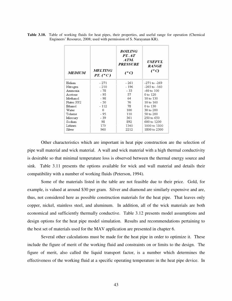
43

Table 3.10. Table of working fluids for heat pipes, their properties, and useful range for operation (Chemical

Engineers’ Resource, 2008; used with permission of S. Narayanan KR).

Other characteristics which are important in heat pipe construction are the selection of

pipe wall material and wick material. A wall and wick material with a high thermal conductivity

is desirable so that minimal temperature loss is observed between the thermal energy source and

sink. Table 3.11 presents the options available for wick and wall material and details their

compatibility with a number of working fluids (Peterson, 1994).

Some of the materials listed in the table are not feasible due to their price. Gold, for

example, is valued at around $30 per gram. Silver and diamond are similarly expensive and are,

thus, not considered here as possible construction materials for the heat pipe. That leaves only

copper, nickel, stainless steel, and aluminum. In addition, all of the wick materials are both

economical and sufficiently thermally conductive. Table 3.12 presents model assumptions and

design options for the heat pipe model simulation. Results and recommendations pertaining to

the best set of materials used for the MAV application are presented in chapter 6.

Several other calculations must be made for the heat pipe in order to optimize it. These

include the figure of merit of the working fluid and constraints on or limits to the design. The

figure of merit, also called the liquid transport factor, is a number which determines the

effectiveness of the working fluid at a specific operating temperature in the heat pipe device. In

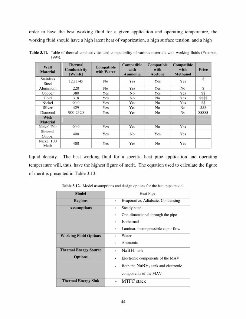
44

order to have the best working fluid for a given application and operating temperature, the

working fluid should have a high latent heat of vaporization, a high surface tension, and a high

Table 3.11. Table of thermal conductivities and compatibility of various materials with working fluids (Peterson,

1994).

Wall Material

Thermal Conductivity

(W/mK)

Compatible with Water

Compatible with

Ammonia

Compatible with

Acetone

Compatible with

Methanol Price

Stainless Steel 12.11-45 No Yes Yes Yes $

Aluminum 220 No Yes Yes No $ Copper 380 Yes No Yes Yes $$ Gold 318 Yes No No Yes $$$$

Nickel 90.9 Yes Yes No Yes $$ Silver 429 Yes Yes No No $$$

Diamond 900-2320 Yes Yes No No $$$$$ Wick

Material

Nickel Felt 90.9 Yes Yes No Yes Sintered Copper 400 Yes No Yes Yes

Nickel 100 Mesh 400 Yes Yes No Yes

liquid density. The best working fluid for a specific heat pipe application and operating

temperature will, thus, have the highest figure of merit. The equation used to calculate the figure

of merit is presented in Table 3.13.

Table 3.12. Model assumptions and design options for the heat pipe model.

Model Heat Pipe

Regions • Evaporative, Adiabatic, Condensing

Assumptions • Steady-state

• One-dimensional through the pipe

• Isothermal

• Laminar, incompressible vapor flow

Working Fluid Options • Water

• Ammonia

Thermal Energy Source

Options • NaBH4 tank

• Electronic components of the MAV

• Both the NaBH4 tank and electronic

components of the MAV

Thermal Energy Sink • MTFC stack

45

Model Heat Pipe

Wall Material Options • Stainless Steel

• Aluminum

• Copper

• Nickel

Wick Material Options • Nickel felt

• Sintered copper

• Nickel 100 mesh

Table 3.13. Equation used to calculate the figure of merit for a working fluid.

Variable Description Model Equation

lρ The liquid density (kg/m3) Given value

λ The latent heat of vaporization (J/kg) Given value

σ Surface tension of liquid (N/m) Given value

lµ Viscosity of the liquid (N·s/m3) Given value

M The figure of merit l

lMµσλρ

=

A final set of calculations, which must be made for a heat pipe, is the determination of

the thermal energy transport limitations. If these limitations are exceeded, the device will fail to

have the proper temperature distribution. This may result in drying out of the wick, complete

evaporation of the working fluid, or a drastic temperature difference between the two ends of the

heat pipe. There are five thermal energy transport limitations which conventionally must be

taken into account. They are as follows:

• Viscous Limit: The maximum thermal energy transport limitation that will allow viscous

forces to not interfere with vapor flow inside the heat pipe.

• Sonic Limit: The maximum thermal energy transport limitation that will allow the vapor

velocity to be subsonic and not exceed a critical or choked flow condition.

• Entrainment Limit: The maximum thermal energy transport limitation that will allow

condensate from the condenser to return back to the evaporator to prevent flooding on

either end.

46

• Capillary Limit: The maximum thermal energy transport limit which is acceptable before

the gravitational, liquid, and vapor flow pressure drops exceed the capillary pumping

head of the wick.

• Boiling Limit: The maximum thermal energy transport limit before nucleate boiling

occurs in the wick structure, resulting in a blockage in the wick and preventing working

liquid from returning back to the evaporator. If this limit is exceeded, the evaporative

section of the heat pipe may dry out.

The model equations for these five limitations are given in Table 3.14 and are based on Peterson

(1994). If the amount of thermal energy transfer from the MAVs thermal energy source is larger

than any of the thermal energy transport limitations listed above, then the heat pipe’ s design must

be altered. For example, the length, diameter, or some other dimension may need to be altered,

or some construction material may need to be changed such as the casing, wick, or working

fluid.

Table 3.14. Model equations for the limitations of a heat pipe heat exchanger (Peterson, 1994).

Variable Description Model Equation

VA Vapor core cross sectional area (m2) Calculated value

oρ Stagnation density (kg/m3) Given value

λ Latent heat of vaporization (J/kg) Given value

vγ Vapor specific heat ratio Given value

vR Vapor gas constant Given value

oT Stagnation temperature (K) Calculated value

sq Sonic limit (W) 2

1

)1(2 ��

�

�

+=

v

ovvoVs

TRAq

γγ

λρ

vd Vapor diameter (m) Calculated value

vP Vapor pressure (N/m2) Given value

vρ Vapor density (kg/m3) Given value

vf Vapor friction factor Given value

vRe Reynolds number Given value

eL Length of the evaporator (m) Calculated value

vµ Vapor viscosity (kg/m·s) Given value

47

Variable Description Model Equation

vq The viscous limit (W) ���

����

�=

vevv

vvvvv Lf

PAdq

µρ

λRe4

2

N Mesh number Given value

σ Surface tension (N/m) Given value

whr , Wick surface pore hydraulic radius (m) Given value

eq The entrainment limit (W) 2

1

,2 ���

�

�=

wh

vve r

Aqσρ

λ

lρ Liquid density (kg/m3) Given value

ψ Heat pipe angle of incidence (degree) Given value

cr Capillary radius (m) Nrc 2

1=

cL Condenser length (m) Given value

aL Length of the adiabatic zone in the heat pipe (m)

Given value

L Length of the heat pipe (m) cae LLLL ++=

mpP , Maximum effective pumping pressure (N/m2)

( ) ( )ψρψρσsincos)2(, gLgd

rP lvl

cmp ++=

eF Liquid friction coefficient Calculated value

vF Vapor friction coefficient Calculated value

effL Effective length (m) eaceff LLLL 5.05.0 ++=

cq Capillary limit (W) eff

ve

mp

c LFF

P

q+

=

,

lk Liquid thermal conductivity (W/m·K) Given value

wk Wicking structure thermal conductivity (W/m·K)

Given value

ε Wick porosity Calculated value

effk Effective conductivity of saturated wick (W/ m·K) ))(1(

)))(1((

wlwl

wlwlleff kkkk

kkkkkk

−−++−−−+

=εε

vT Vapor temperature (K) Given value

ir Inner radius (m) Given value

vr Vapor radius (m) Given value

nr Nucleation radius (m) Given value

48

Variable Description Model Equation

bq Boiling limit (W) ��

�

�−=

cnviv

veffeb rrrr

TkLq

σσλρ

π2

2)ln(

2

3.6 iSCRIPT™ The model for the MAV power plant and its multiple components was implemented

using iSCRIPT™. iSCRIPT™ is a computer programming and scripting language developed by

TTC Technologies with the help of Dr. Ken Alabi. The language was created to model various

engineering systems with a focus on optimization. iSCRIPT™, unlike other programs, identifies

the optimal conditions for the system. In the previous research phase, only a MTFC was

modeled for the MAV. For this thesis research and phase, the remainder of the MAV power

plant system was modeled and optimized to determine materials, size, and other necessary

properties required to manufacture the system.

Each subsystem mentioned throughout this chapter was modeled using the iSCRIPT™

language with a scripting program called Crimson Editor. All possible options regarding

manufacturing materials, length, etc. were placed into the program. The programs for each of

these subsystems then determined which sequence of options created the most optimal

performing subsystem. Some values, such as the heat pipe length, are user-input values because

they must be constrained to the dimensions of the MAV or their assigned compartments.

49

4 Chapter Four - Experimental Setup and Testing A primary focus of this research was the construction and experimental testing of

individual MTFCs as well as a stack. Combined with the analytical modeling of Chapter 3, a

prototype design of the fuel cell stack system for implementation in a MAV was realized.

4.1 Description of an MTFC The MTFC is a fuel cell that is geometrically tubular and made from small Nafion®

tubing, planar Nafion® membrane extruded into a tubular form. The fuel cell generally varies in

length and is covered in a catalyst ink. The catalyst ink covers both the interior and exterior of

the cell with a thick layer. On either end of the fuel cell, two gas delivery needles are connected

to the cell, and are done so with the use of a two-part epoxy (often made from Loctite®). Figure

4.1 is a schematic of a MTFC made during the previous phase with only the catalyst ink applied

and stainless steel gas dispersion needled attached. The stainless steel gas delivery needles, as

shown, are simply syringe-like metallic needles that are wider than those used in medicine. The

anode gas delivery on the left side of the figure serves as an exit channel for unused hydrogen

gas and water to leave the MTFC.

Figure 4.1. A tubular PEMFC (i.e., MTFC) fabricated in 2007 during the previous phase with mechanical parts labeled.

Before the catalyst ink is applied to the MTFC, the anode collection layer is placed inside

the cell. This is usually a wire that is coiled tightly so that it can be placed inside the fuel cell.

To coil a wire, a small, 19 or 20 gage rod extending no longer than a foot is place into a drill

chuck and set in place. If the rod is diametrically too small for a chuck, a small piece of sizing

foam or scotch tape is placed at the rod’ s inner tip. The coil is made by taping one end of the

50

wire spool to the drill chuck, holding the remaining wire exposed in your hand as if sewing. The

drill is turned on gently and the wire is glided around the now rotating rod until a coil of a

desired length if completed. If the gold or metallic coil can not be placed inside the Nafion®

tubing, the tubing is soaked in liquid methanol. Because of its chain-link chemistry, Nafion®

membrane absorbs methanol to expand, causing the tubular inner diameter to expand. Once

expanded, a wire coil can be placed inside the tube. The tube is then dried on a towel so that it

can shrink back to its original size.

After anode collection (or conduction) layer insertion and catalyst ink application, the

cell is often covered with cathode collection layer. Often this is carbon nanofiber (CNF)

threading which is wrapped around the MTFC entirely. Figure 4.2 is a schematic picture of a

MTFC fabricated in early 2009 during the present phase. The cell is covered in two cathode

collection layers: a carbon nanofiber wrap and gold cathode collection wire. Nearly all MTFCs

were fabricated with a cathode collection layer of some type; more information about this is

discussed in a later section.

Figure 4.2. MTFC schematic after fabrication. Once the MTFC has been fabricated, the cell will have a mechanical structure like the

schematic presented in Figure 4.3, which shows the various layers of a tubular fuel cell after it

has been fabricated. These layers include the conduction layers just mentioned, cathode and

anode, with its catalyst ink, and the Nafion® polymer. The hydrogen gas flows through the

51

interior and reacts on the catalyst surface, following which the protons are transferred through

the membrane and the electrons through the conduction layer to a circuit board.

Figure 4.3. Cross sectional schematic of a MTFC.

4.2 General Test Procedures

MTFCs are tested somewhat differently than conventional flat plate PEMFCs. Like flat

plate fuel cells, they are tested using potentiostatic, potentiodynamic (polarization), and

electrochemical impedance spectroscopy test facilities such as those at the Sustainable Energy

Lab at the Institute for Critical Technology and Applied Sciences (ICTAS) which includes a Fuel

Cell Technologies® (FCT) test station. However, MTFCs are not tested between two graphite

plates containing serpentine gas delivery channels in a plate format. Instead, rubber hoses are

connected from the test station, using luer locks, to the gas dispersion needles mentioned

previously. The rubber gas tubes supplying the fuel are attached to the needle ends, allowing

hydrogen or inert N2 purge gas to flow freely through the anode section of the MTFC. A picture

of the fuel cell test station with its anode and cathode gas supply lines labeled is presented in

Figure 4.4. Figure 4.5 is a schematic of a MTFC with the gas inlet and outlet channels labeled.

As can be seen, the anode gas flows through the interior of the cell and air passively flows

around the outside cathode side. Rubber tubing connects both ends of the MTFC to the supply

lines of the test station. A computer is attached to the test station to adjust gas flow, humidity,

and temperature.

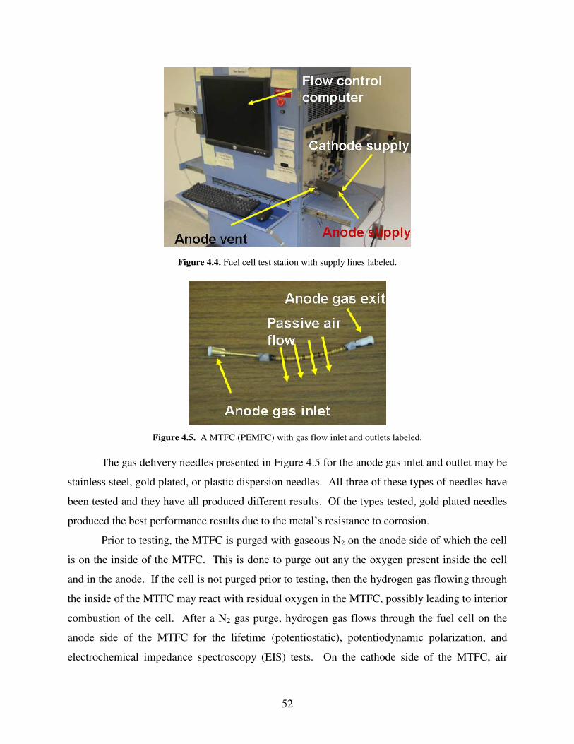
52

�

Figure 4.4. Fuel cell test station with supply lines labeled.

Figure 4.5. A MTFC (PEMFC) with gas flow inlet and outlets labeled.

The gas delivery needles presented in Figure 4.5 for the anode gas inlet and outlet may be

stainless steel, gold plated, or plastic dispersion needles. All three of these types of needles have

been tested and they have all produced different results. Of the types tested, gold plated needles

produced the best performance results due to the metal’ s resistance to corrosion.

Prior to testing, the MTFC is purged with gaseous N2 on the anode side of which the cell

is on the inside of the MTFC. This is done to purge out any the oxygen present inside the cell

and in the anode. If the cell is not purged prior to testing, then the hydrogen gas flowing through

the inside of the MTFC may react with residual oxygen in the MTFC, possibly leading to interior

combustion of the cell. After a N2 gas purge, hydrogen gas flows through the fuel cell on the

anode side of the MTFC for the lifetime (potentiostatic), potentiodynamic polarization, and

electrochemical impedance spectroscopy (EIS) tests. On the cathode side of the MTFC, air

53

flows either passively or through a hose into a humidity chamber allowing the gas to effectively

reach the external cathode side of the cell. The volumetric flow rate of hydrogen into the MTFC,

although typically 100 standard cubic centimeters per minute (sccm), is a testing variable which

may alter the performance of a cell. Air on the cathode side typically flows at 3000 sccm when

through the hose into the humidity chamber. Otherwise, it flows passively around the outside of

the MTFC by simply being in an ambient environment. A picture of the MTFC hooked up to the

fuel cell test station and inside a relative humidity chamber is shown in Figure 4.6.

Figure 4.6. An MTFC attached to the fuel cell test station. This cell has been placed in a humidity chamber.

When tested, two wires connect to the anode and cathode side of the MTFC by means of

two alligator clips. This is done to run the various tests on the cell as mentioned previously.

Figure 4.7 presents a schematic of how the alligator clips connect to the MTFC and attached to a

potentiostat external to the fuel cell test stand. Normally the current and voltage would be

measured using the FCT test station. However, the FCT potentiostat circled in Figure 4.6 is not

sensitive enough to measure the low current and voltage values of the MTFCs developed here.

Thus, these electrical properties are measured the external Solartron® Model 1480 8-channel

potentiostat shown in Figure 4.7 The MTFC is, therefore, attached both to the FCT for gas flow,

relative humidity, and control and to the external potentionstat and its accompanying software

Corrware™ and Z-plot™. These programs collect data from the Solartron device, graphically

interpret it, and generate the lifetime power density and polarization curves (Corrware™) and

EIS curves (Z-plot™). More than two hundred MTFCs have been tested in this way.

54

Figure 4.7. The Solartron® Model 1480 8-channel potentiostat and its connection to the MTFC.

When tested, the MTFCs are placed in two vice grips at an angle lower than 45° or

completely vertical when in the humidity chamber. When the MTFC is in a humidity chamber

as shown in Figure 4.6, the wires go out of the chamber through holes in a rubber stopper at the

top of the chamber. A detailed schematic of the cell in the humidity chamber with various gas

hoses labeled is presented in Figure 4.8. In the testing orientation, the cell is attached to rubber

tubing and luer locks allowing H2 gas to flow on the anode side of the MTFC. Rubber tubing

also supplies air on the cathode side of the MTFC at a flow rate of around 3000 sccm, filling up

the chamber until a desired RH is achieved for the air. For each MTFC, the testing process takes

approximately 50 minutes.

The three tests previously mentioned are used to capture various qualities of the fuel cell,

and are tested differently. The lifetime test is used to determine how the cell recovers given an

applied load (set by a constant voltage, typically 0.3 v for this research) over a long period of

time. Using Corrware™, a time is also set for the test (i.e, 30 min, 2 hours), and data point are

typically taken every few seconds (this may also be set). A polarization test is conducted to

determine the overall performance of the fuel cell, its efficiency, open circuit voltage, and

55

associated losses (by inspection of the data). Using Corrware™, the test is applied with

changing voltage and current to create a polarization curve. Finally, an EIS test is conducted to

find the amount of resistance associated with the cell by producing a Nyquist plot of real and

imaginary impedance. Before the test commences, two values are applied to the Z-plot™

program: a DC voltage and a range for AC current. The DC voltage set is ½ the maximum OCV

value observed for the cell, and the AC current range is roughly ½ the DC voltage value, but is

dependent on the results of the polarization curve. Also, a frequency is set to test the EIS which

vary from 1 kHz to100 kHz.

Figure 4.8. The chamber with a MTFC connected to the fuel cell test stand.

4.3 Micro-Tubular Cell Construction Improvements

Over the course of this research, much has been discovered regarding factors affecting

the voltage and current of the MTFCs in testing and polarization studies. One of the biggest

factors affecting performance is the method of construction. Various changes to the original

manufacturing steps have been made to determine if they are effective at increasing the power

density or current density of the tubular fuel cell. These include the material composition and

coating of the anode gas dispersion needles, diameter of the tubular Nafion® (TT-030, TT-050,

56

TT-060 or TT-110), the catalyst layer ink formula, the anode and cathode conduction layer and

collector, cell length, and the processing steps during manufacture. Some of these factors had

great impacts on the MTFC’ s open circuit voltage (OCV) and power density whereas others did

not.

4.3.1 Nafion® Membrane

As with any PEMFC, the polymer membrane is vitally important to achieving the power,

voltage, and current of the fuel cell. The thickness of the Nafion® membrane is important with

respect to proton transport, water management, and fuel crossover, regardless of whether the fuel

cell is planar or tubular. Nafion® membranes produced by Perma Pure LLC are sold at various

wall thicknesses. The wall thickness, inner diameter, outer diameter, internal volume, and

weight specifications for different product numbers are shown in Table 4.1 (Perma Pure, 2009).

A picture of the Nafion® tubing (product number TT-060) after being soaked in deionized water

is presented in Figure 4.9.

Table 4.1. The Nafion® membrane tubing specifications for different model numbers (Perma Pure, 2009).

Model Number Inner Diameter Outer Diameter Wall Thickness

TT-030 0.025 in 0.033 in 0.004 in

TT-050 0.042 in 0.053 in 0.005 in

TT-060 0.052 in 0.063 in 0.006 in

TT-070 0.060 in 0.072 in 0.006 in

TT-110 0.086 in 0.108 in 0.012 in

Figure 4.9. A tube of TT-060 Nafion® after being heated in deionized water.

57

Of the different Nafion® tubes presented in the table, all of them were used to

manufacture the MTFCs tested. Of these product numbers, MTFCs manufactured using TT-060

overall performed the best with respect to power and current density. Due to the performance,

reliability, and durability of the MTFCs manufactured with TT-060 type Nafion®, this tubing is

used to fabricate the fuel cells for the stack prototype. A performance comparison between the

MTFCs made from TT-060 and other types of Nafion® is presented in Chapter 6.

4.3.2 Catalyst Layers and Methods of Application

One important characteristic of the fuel cell which impacts performance regardless of

type is the catalyst layer, its application, formulation, and manufacture. It is well known in the

fuel cell industry that both the application of a catalyst layer and its formulation are equally

important to the success of a fuel cell. Jim Klocke, senior business development manager of

Asymtek®, a California-based jet and ink dispensing equipment company, said “ the success of

the catalyst ink depends 50% on its chemistry and 50% on its application (Asymtek®, 2007).”

Anyone conducting research in fuel cell science would concur with him that loading and ink

chemistry play equal roles in fuel cell performance, regardless of its geometry. In this research,

both application and formulation are varied for MTFC fabrication. The science behind these two

process steps, as well as how they are varied in this research, are discussed in the following

sections.

������� ������� �������� �������

Traditionally for PEMFCs, the catalyst ink is made from platinum on carbon black

powder (or for DMFCs, platinum-ruthenium powder), ethylene glycol, and Nafion® solution.

Once these are mixed together in desirable proportions, the solution is then heated at a desired

temperature and placed in a sonic bath or sonicated using, for example, a Biologics, Inc. Model

300 V/T Ultrasonic Homogenizer. The ink is sonicated so that colloidal suspension is broken up

to achieve a desirable viscosity and effectiveness. Colloidal suspension is, essentially, the

indefinite suspension of particles which may be solid or liquid within a substance of a different

phase. Sonication breaks up the particle agglomerates and prevents them from settling, making a

58

more uniform suspension. Sonicated ink should improve the catalyst layer whether for planar or

tubular PEMFCs or DMFCs.

Much care must be taken when creating the catalyst ink. A desired viscosity so that it can

bind to the fuel cell well is only part of the battle. The following requirements must be met when

formulating the catalyst ink in order for it to be effective:

• The catalyst layer should have a high mechanical strength

• The catalyst layer should be highly conductive electrically

• The catalyst layer should not easily corrode

• The catalyst layer should be fairly easy to apply

• The catalyst layer should have a high catalytic activity (a high exchange current)

It is because of these factors that the research efforts conducted at Virginia Tech have focused on

varying the catalyst ink formulation. In order to meet the above criteria and produce an ink

which is effective in catalyzing the electrochemical reactions and producing the best current and

power densities. Several variations have been created of the catalyst ink for this research. The

variations include:

• Altering the Nafion® solution content of the ink

• Varying the catalyst (Pt) loading

• Adding Pyrograph vapor grown carbon nanofiber (CNF) to the ink formula and

varying its weight percentage

• Varying the type of Nafion® solution in the ink formula (1000 or 1100

grams/equivalent equivalent weight of perflourinated resin in the Nafion® solution

(Gierke et al., 1982))

• Varying the duration of ink sonication

• Introducing E-fill (a nickel based conductive filler) into the catalyst ink, and varying

its concentration

These variations affect electrical conductivity, mechanical strength, adhesion to the membrane

wall, etc. For example, nickel E-fill is introduced into the formulation of the catalyst ink in order

to improve electrical conductivity within the catalyst layer. Altering the type and amount of

Nafion® solution affects the adhesion of catalyst ink onto the membrane; adding Pyrograph

59

vapor grown CNF plays a role in the mechanical strength of the ink, its electrical conductivity,

and the number of active reaction sites; and changing the catalyst loading increases the number

of reaction sites. A breakdown of how the catalyst ink formulation is varied can be seen in

Appendix A. The results from testing the MTFCs using these variations are presented in Chapter

6.

������� ������� ���������������

Because the catalyst promotes the electrochemical reactions, successful and uniform

application of catalyst ink determines the effectiveness of the electrochemical process, which

produces current and power from the cell. Thus, care needs to be taken in applying the catalyst

layer to the membrane. Too much catalyst ink may lead to a reduction of triple phase boundaries

(TPB) present due to a reduction of gas pores exposed to the polymer of the PEMFC. TPBs are

the sites in the catalyst layer where electrochemical reactions occur because they are locations

where the three important phases, Nafion®, gas, and electrically and ionically connected catalyst

meet. Too little application of catalyst layer may also result in a reduction of the number of TPB

points present, leading to insufficient electrochemical activity within the electrodes (O’ Hayre et

al., 2006). Therefore, extreme caution must be taken when applying catalyst ink to the Nafion®

membrane of the MTFC. Figure 4.10 is a schematic of the catalyst layer/electrolyte interface

and the TPBs.

Figure 4.10. A schematic of the catalyst layer/electrolytic membrane interface of the fuel cell. The TPBs are

shown in this figure and clearly represent the point at which all three phases meet.

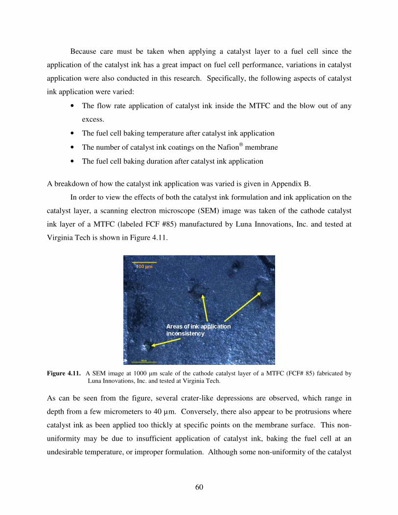
60

Because care must be taken when applying a catalyst layer to a fuel cell since the

application of the catalyst ink has a great impact on fuel cell performance, variations in catalyst

application were also conducted in this research. Specifically, the following aspects of catalyst

ink application were varied:

• The flow rate application of catalyst ink inside the MTFC and the blow out of any

excess.

• The fuel cell baking temperature after catalyst ink application

• The number of catalyst ink coatings on the Nafion® membrane

• The fuel cell baking duration after catalyst ink application

A breakdown of how the catalyst ink application was varied is given in Appendix B.

In order to view the effects of both the catalyst ink formulation and ink application on the

catalyst layer, a scanning electron microscope (SEM) image was taken of the cathode catalyst

ink layer of a MTFC (labeled FCF #85) manufactured by Luna Innovations, Inc. and tested at

Virginia Tech is shown in Figure 4.11.

Figure 4.11. A SEM image at 1000 �m scale of the cathode catalyst layer of a MTFC (FCF# 85) fabricated by

Luna Innovations, Inc. and tested at Virginia Tech. As can be seen from the figure, several crater-like depressions are observed, which range in

depth from a few micrometers to 40 µm. Conversely, there also appear to be protrusions where

catalyst ink as been applied too thickly at specific points on the membrane surface. This non-

uniformity may be due to insufficient application of catalyst ink, baking the fuel cell at an

undesirable temperature, or improper formulation. Although some non-uniformity of the catalyst

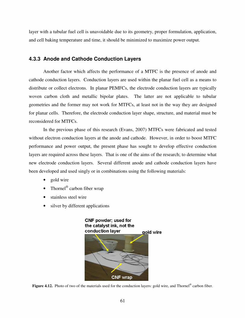
61

layer with a tubular fuel cell is unavoidable due to its geometry, proper formulation, application,

and cell baking temperature and time, it should be minimized to maximize power output.

4.3.3 Anode and Cathode Conduction Layers Another factor which affects the performance of a MTFC is the presence of anode and

cathode conduction layers. Conduction layers are used within the planar fuel cell as a means to

distribute or collect electrons. In planar PEMFCs, the electrode conduction layers are typically

woven carbon cloth and metallic bipolar plates. The latter are not applicable to tubular

geometries and the former may not work for MTFCs, at least not in the way they are designed

for planar cells. Therefore, the electrode conduction layer shape, structure, and material must be

reconsidered for MTFCs.

In the previous phase of this research (Evans, 2007) MTFCs were fabricated and tested

without electron conduction layers at the anode and cathode. However, in order to boost MTFC

performance and power output, the present phase has sought to develop effective conduction

layers are required across these layers. That is one of the aims of the research; to determine what

new electrode conduction layers. Several different anode and cathode conduction layers have

been developed and used singly or in combinations using the following materials:

• gold wire

• Thornel® carbon fiber wrap

• stainless steel wire

• silver by different applications

Figure 4.12. Photo of two of the materials used for the conduction layers: gold wire, and Thornel® carbon fiber.

62

Figure 4.12 shows two of the materials which are used for the electrode conduction

layers. A third material, CNF powder, is pictured in this figure. However, CNF powder is used

to modify the catalyst ink and not the conduction layer of the MTFC. Of the cells created by

Luna Innovations and Virginia Tech, the majority of them were manufactured with gold wire as

the anode collector (i.e. conduction layer) and gold wire and Thornel® carbon fiber wrap as the

cathode conduction layer. The wires used were typically manufactured by MWS Wire

Industries. When a cell is prepared, the carbon fiber wrap is wrapped around the coated and

dried cell until full coverage is observed. After the thread ends have been taped to gas delivery

needles, gold wiring is wrapped tightly around the cell from end to end with extra wire hanging

off the end of the shorter gas delivery needle. A picture presenting a cell after this process was

shown in Figure 4.2.

4.4 Testing Variables and Conditions Just as the fabrication method affects the power output and performance of the fuel cell,

so too does the condition of the fuel cell, which in a MAV, can vary from the standard test

conditions used with the fuel cell test station at Virginia Tech. In particular, the temperature and

relative humidity of the air surrounding the MTFC stack and supplied to the cathode can vary

quite a bit. Other conditions, which are external to the fuel cell but ultimately affect its

performance, include the hydrogen gas volumetric flow rate, “ dead ending” of the MTFC, and

the passage of time (called cell conditioning). These conditions in particular as well as how to

simulate them, are discussed in the following sections.

4.4.1 Relative Humidity

The relative humidity (RH) is an important condition, which affects MTFC performance.

RH is important to a MTFC particularly because of the Nafion® membrane utilized. Nafion® is

often referred to as a perflourosolfonic acid (PFSA) membrane, a type of membrane whose

conductivity is highly dependent on its water content. Therefore, having a high RH around the

fuel cell prevents the membrane from losing moisture and as a consequence reducing its

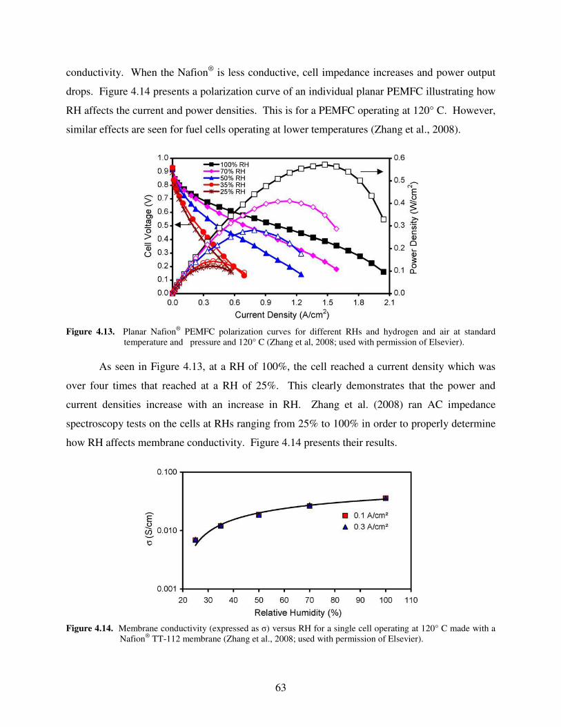
63

conductivity. When the Nafion® is less conductive, cell impedance increases and power output

drops. Figure 4.14 presents a polarization curve of an individual planar PEMFC illustrating how

RH affects the current and power densities. This is for a PEMFC operating at 120° C. However,

similar effects are seen for fuel cells operating at lower temperatures (Zhang et al., 2008).

Figure 4.13. Planar Nafion® PEMFC polarization curves for different RHs and hydrogen and air at standard

temperature and pressure and 120° C (Zhang et al, 2008; used with permission of Elsevier). As seen in Figure 4.13, at a RH of 100%, the cell reached a current density which was

over four times that reached at a RH of 25%. This clearly demonstrates that the power and

current densities increase with an increase in RH. Zhang et al. (2008) ran AC impedance

spectroscopy tests on the cells at RHs ranging from 25% to 100% in order to properly determine

how RH affects membrane conductivity. Figure 4.14 presents their results.

Figure 4.14. Membrane conductivity (expressed as �) versus RH for a single cell operating at 120° C made with a

Nafion® TT-112 membrane (Zhang et al., 2008; used with permission of Elsevier).

64

In order to simulate a varying relative humidity environment for the MTFCs, a RH

chamber was constructed. The chamber is a 4 liter Erlenmeyer flask stopped with a rubber

stopper allowing gas flow to enter and exit the chamber and fuel cell. A picture of the chamber

was shown in Figure 4.8.

To monitor the RH and operating temperature within the chamber, a Vaisala HUMICAP®

humidity and temperature transmitter HMT337 is used (see figure 4.15). Traditionally, this

device is used to measure meteorological data. A picture of the measuring device is shown

below. For testing of MTFCs, the RHs of the chamber are varied from 2% RH to 100% RH.

Figure 4.15. The Vaisala HUMICAP® humidity and temperature transmitter HMT337 (Vaisala, 2009; photo courtesy of Vaisala Inc.).

4.4.2 Hydrogen Flow Rate Hydrogen flow rate is an important aspect that affects the performance of the fuel cell.

This is because flow rate is the fuel supply rate to the cell, the driving force for the entire

electrochemical reaction. When individual fuel cells are tested, a mass flow controller sets the

hydrogen flow rate being supplied to the anode side of the MTFC. The Fuel Cell Technologies,

Inc. test stand used at Virginia Tech has a mass flow controller so that hydrogen anode and

cathode gas volumetric flow rates can be set. Typically, hydrogen flows through the tubular fuel

cell at 100 sccm. Given that the density of the hydrogen is 0.0899 g/l, or 0.0000899 g/cm3, the

mass of hydrogen supplied over one hour is 0.54 g. The volumetric flow rates for hydrogen used

ranged from 25 sccm to 125 sccm. The mass of hydrogen used for each flow rate is given in

Table 4.2.

65

Table 4.2. Varying hydrogen flow rates and the hydrogen mass supplied per hour for each.

Hydrogen flow rate (sccm)

Mass of Hydrogen supplied in one hour (g)

25 0.14 50 0.27 75 0.40

100 0.54 125 0.67

It is important to understand what a desired flow rate should be for a MTFC so that

enough hydrogen is being supplied to the anode side of the cell. If a low flow rate results in an

insufficient amount of hydrogen, then the MTFC can not reach the power level needed.

Conversely, if a higher than necessary volumetric flow rate of hydrogen is used, then NaBH4 in

the hydrogen storage tank is wasted, and a risk is taken of potentially damaging the cell structure.

Thus, the hydrogen flow rate was varied during the MTFC tests to determine how the power

output changes. Recommendations for hydrogen flow rate are discussed in Chapter 6.

66

5 Chapter Five - Prototype Development and Testing In the course of this research, a prototype fuel cell stack was designed and constructed in

order to house a set of MTFCs. The principal material used for the prototype structure is white

Teflon®, which holds the MTFCs together, while also allowing hydrogen gas to properly flow

through their anode channels. In addition, the prototype allows for air to passively flow around

the cathode exterior of the fuel cells by assuring sufficient space between each individual cell. It

should be notes that the prototype dimensions will be presented in English units, not SI. This is

to allow one to better visualize the design relative to the dimensions provided by the U.S. Air

Force without the need for unit conversion.

5.1 Prototype MTFC Stack Design The prototype structure has a tri-circular MTFC stack arrangement with two cylindrical

enclosures on either end, housing entering and exiting fuel gas. Each enclosure is 1.68 in long

and has a diameter of 3.25 in. The prototype was chosen to be cylindrical to more efficiently

accommodate a large quantity of MTFCs and to allow gas to flow effectively through the stack.

The prototype structure is also equipped with two separation discs, which are used as structural

bumpers between the individual cells. The prototype structure was designed using Autodesk

Inventor™ and constructed by the mechanical engineering machine shop at Virginia Tech. All

the machined parts of this structure are shown in Figure 5.1.

The prototype structure designed can accommodate forty MTFCs in a circular

arrangement which fits within the 3.25 in diameter of the end enclosures. The circular MTFC

arrangement has a diameter of 2.75 in. The remaining 0.5 in is used to anchor parts of the

prototype structure together, providing structural rigidity. The largest two parts of the prototype

structure are the cylindrical tanks, which serve as inlet and outlet enclosures for hydrogen gas

and are sealed off to prevent leakage by a Teflon® disc, rubber O-ring, and silicon gasket

(depending on the tank). The enclosure on the top left of Figure 5.1 is sealed closed, while the

one to the right is left open to demonstrate how the hydrogen gas enclosures are sealed shut for

assembly. Each enclosure has a hole with a depth 0.375 in into the part which is 0.25 in smaller

67

in diameter than that of the enclosure. This is done for purposes of mating the mechanical

components needed, and a small Teflon® disc into the enclosure to seal it tight and prevent

hydrogen gas leaks. The open enclosure presented in Figure 5.1 has a rubber O-ring placed snug

inside the hole.

Figure 5.1. The prototype structure disassembled and labeled.

To the right of the open enclosure are two discs with forty holes arranged in three circular

configurations. These discs are referred to as separation discs and measure 3.25 in in diameter

and are 0.125 in thick. They are used to assure a proper spacing between individual MTFCs and

the structural stability of the prototype. There are four outer holes in the disc as well, each0.125

in in diameter and 90° from the nearest neighbor. They are used for elongated screws, which

align the discs with the prototype structure and aid in the stability of the fuel cell stack. The

outermost configuration of the three circular configurations consists of 16 holes, each equally

spaced apart. The middle circular configuration also has 16 holes and an equal spacing, but

rotated counterclockwise 11.25° to the outermost configuration. This produces a staggering

effect for the tubular cells, allowing air to flow more freely through the stack. The innermost

circular configuration has only eight holes, equally spaced apart by 45°. With a diameter of 0.20

in, each hole is large enough to accommodate a single tubular cell with additional space

68

remaining. Note that the forty hole configuration described applies to all Teflon® discs that are

used to hold tubular fuel cells or their hydrogen gas delivery needles in place within the

prototype structure. An Inventor™ drawing of the separation disc is displayed in Figure 5.2.

Figure 5.2. Inventor™ drawing of a separation disc used in the prototype.

In addition to the separation discs, four Teflon® plates were fabricated for the prototype

structure, two with a 2.75 in, and two with a 3.25 in diameter. On these four plates, 40 holes

measuring 0.042 in in diameter (roughly equal to that of a 19 gage needle) each are drilled as

shown in Figure 5.3 and 5.4 in the exact same configuration as that of the separation discs

discussed previously. These holes are used to hold hydrogen delivery (or dispersion) needles

epoxied to the tubular fuel cells in place within the prototype. The purpose of these four discs

is, thus, to guarantee rigidity in the stack and to help prevent gas escaping from any of the

prototype enclosures. The diametrically smaller two plates seen in Figure 5.4 are mated with the

enclosure in the hole, while the larger plates are placed on the open-ended surface of the

enclosures to serve as a “ closing lid” for the two end tanks. The larger plates, shown in Figure

5.3 and in the center of Figure 5.1, have eight 0.125 in diameter holes along their outer edge, as

well as 40 small 0.042 in diameter holes for hydrogen gas delivery needles to pass through them.

Four of these holes are used as screw holes to anchor and align all other parts of the prototype

(such as the separation plates and opposing enclosure), while the remaining four holes seal the

smaller plates, rubber O-rings, and/or silicon septum into the end enclosures. The definition of

69

the discs and O-rings and how they are placed in the prototype structure, apply to only the end

enclosure where hydrogen gas is entering the prototype structure.

The enclosure on the opposite side of the prototype structure has an arrangement that is

very similar to the other, with a few exceptions. On this end of the prototype structure, a large

Teflon® sealing disc is used as discussed previously to seal the enclosure, and a small Teflon®

sealing disc is placed inside the enclosure to anchor the 40 hydrogen gas delivery needles in

place. However, since there is not a great concern for gas leakage in the exiting end of the

prototype stack, considering that this spent gas is no longer used, a silicone septum to prevent

leaking is not inserted into this enclosure. A silicone septum is, however, placed inside the

Figure 5.3. Inventor™ drawing of the large Teflon® sealing disc.

opposite enclosure. Instead, it is simply replaced in the exiting enclosure with a rubber O-ring,

meaning that two O-rings and the small Teflon® sealing disc are the only parts inserted in the

exiting enclosure. The opposite enclosure of the prototype structure only utilizes one O-ring to

assemble. An Inventor™ drawing of the 0.125 in thick silicone septum is presented in Figure

5.5. No holes are drilled into the silicone septum for the hydrogen delivery needles because they

can be pushed through it with ease if sharpened with a bench grinder.

70

Figure 5.4. Inventor™ drawing of the small Teflon® disc for the hydrogen delivery needles.

Figure 5.5. Inventor™ drawing of the silicone septum placed inside the entering hydrogen gas enclosure.

As stated in Chapter 2, in order for the prototype fuel cell stack to function correctly and

allow a sufficient flow of air to the MTFC cathodes, the MTFCs must have an individual

separation of at least 0.51 mm (0.020 in) (Kimble et al., 2000). The prototype allows for a

separation of this distance and greater as illustrated in the schematic of Figure 5.6.

Another part of the prototype stack is the electrical circuit disc. It is shown in Figure 5.7.

This is a printed circuit (PC) board, which is used to electrically connect the MTFCs’ electrical

connections in series. The PC board is 2.75 in in diameter and etched, using PCB etchant

71

solution, from a 2-sided copper-clad PC board (available at Radio Shack) to create a circular

series circuit for the fuel cell connections. In the circuit, the anode wire of one fuel cell is

Figure 5.6. Schematic illustrating the separation distances between MTFCs in the prototype stack.

Figure 5.7. The electrical PC board shown in the prototype structure.

connected to the adjacent cell’ s cathode connection, and is repeated until all fuel cell electrical

connections are formed into a series circuit as shown in the schematic of Figure 5.8.

An anode connection of a cell on the outermost circular assembly and a cathode

connection of a cell on the innermost circular assembly are left unconnected and serve as the

power supply wire for the MAV. Etching and creating a circuit for a circular fuel cell

72

arrangement is quite difficult given that forty cells must be connected in series in a 5.94 in2 area.

The circuit was etched using transfer paper and the design of Figure 5.8 so that only copper

connections remained in a circular fashion, beginning with the outermost cell configuration and

connecting to the middle and inner configurations. The anode and cathode wire ends are

connected to the copper circuitry on the electrical disc by creating solder points. The disc is

Figure 5.8. Electrical circuit of the printed circuit board placed in the prototype structure.

anchored to the rest of the prototype with the help of the hydrogen gas delivery needles of the

MTFCs in the stack. The needles are inserted through holes in the electrical disc and into the

enclosure tank as illustrated in Figure 5.7.

Once the electrical disc is put in place and soldered to the MTFCs, the hydrogen gas

delivery needles are inserted in the gas entry and exit tanks, and the tubular fuel cells are in the

stack, the prototype assembly can be finished. Figure 5.9 is an Autodesk Inventor™ depiction of

the MTFC prototype assembled and ready for installation into the MAV. Figure 5.10 is a labeled

depiction of the prototype exploded to provide a pictorial assembly guide in the event that any

part of the device needs to be repaired.

73

If needed, a desiccant disc can also be placed inside the gas entry enclosure to ensure a

drop in RH of the hydrogen gas flowing into the fuel cell stack. How much desiccant needed is

predicted by the system model, results for which are presented in Chapter 6.

Figure 5.9. Drawing of the prototype and forty tubular fuel cells in the stack.

Figure 5.10. Labeled design of the fuel cell stack prototype disassembled.

A partial assembly of the prototype stack with four MTFCs is displayed in Figure 5.11.

The prototype after it has been assembled is approximately 11.74 in in length and occupies a

volume of 97.4 in3. The total mass of the prototype structure is 765.0 g with 40 cells in the stack.

74

In mass and dimension, the prototype structure is too large for some MAVs but ideal for others.

If this were to be placed into the Dragonfly MAV given its wingspan of only 12 in and a mass of

186 g, it would not be able to fit and would be too heavy for the aircraft. It would, on the other

Figure 5.11. The prototype with six MTFCs installed and connected to the PC board on the left side of the device.

Figure 5.12. An MAV with individual fuel cells placed in a “ wingbone” like arrangement.

hand, fit inside the Top I Vision Casper 200/250 UAV with room to spare since it has a

wingspan of 78.74 in and a mass of 2.3 kg. However, it should be emphasized that the prototype

stack developed here with the limited time and resources available is simply that, a prototype,

75

which serves as a mockup of the cell stack which might be implemented in an MAV. Further

research and development is, thus, needed to realize the power and size requirements initially

envisioned. Furthermore, given the high quantity of MTFCs needed, an expanded application of

the cells throughout the wings (a “ wingbone” arrangement) and body of the aircraft as illustrated

in Figure 5.12 may be needed.

5.2 Prototype MTFC Stack Testing Once the MTFCs are installed into the prototype structure, testing using the fuel cell test

station can begin. The prototype structure is tested by being placed in a humidity chamber,

which allowins the cathode air to maintain a specific RH. Rubber hoses are then run from both

sides of the fuel cell test station and joined together to be placed inside the humidity chamber.

The hoses running from both anode outlets carrying hydrogen are joined, inserted into the

humidity chamber through a hole in it, and into a hole in the prototype’ s gas entry enclosure with

the help of a luer lock. The hoses running from both the cathode vents of the fuel cell test station

carrying humidified air are joined and inserted into a hole in the humidity chamber. The air

being supplied to the chamber simply fills the chamber with enough gas to sufficiently supply

the cathode sides of the prototype MTFCs. Excess hydrogen gas leaving the prototype does so

with the help of a single outlet tube running from a hole in the prototype exit enclosure through

another hole of the humidity chamber, and to the anode vent connection of the test station.

Figure 5.13 is a schematic of the prototype testing setup.

The prototype is also tested in another configuration. When individual prototype

intended cells are chosen, they are placed next to each other on a plastic slab and hinged to it

with tape in a parallel configuration. Wires from the anode side of the MTFC are wrapped with

the adjacent cells cathode wire, and repeated in such a manner until all cells are connected

electrically in a circuit. The anode gas delivery needles of the cells are inserted into a universal

plastic tube, which supplies hydrogen to the stack. The cells are left open-ended so that unused

76

Figure 5.13. Schematic of the prototype structure attached to the test stand ready for experimentation.

Figure 5.14. Schematic of a prototype testing setup testing 12 MTFCs in series. H2 can exit the cells into a ventilation device. The series connections made between these cells

are attached to the potentiostat for testing. A schematic of this prototype testing setup is

presented in Figure 5.14.

77

6 Chapter Six - Results and Discussion

After modeling the MTFC system, conducting electrical tests on many MTFCs, and

testing the MTFC stack prototype, many numerical results were found. Some of the results

found were inconclusive, while others gave clear distinctions as to which fabrication method

creates the best performing cells. This chapter presents the results of testing conducted on

individual fuel cells and the prototype and results from the computer program model of the fuel

cell system. Additional discussion will also be presented in this chapter regarding fuel cell stack

creation and implementation into an MAV and recommendations.

6.1 Mathematical Model Results

The sections to follow present numerical results of the iSCRIPT™ computer model

simulations of the fuel cell stack and balance of plant components of the MTFC system. These

include numerical results for the NaBH4 hydrogen gas storage tank, desiccant disc for gas RH

control, energy storage capacitor, and heat pipe heat exchanger. These components are

combined together with the fuel cell stack to produce the entire power supply system for the

MAV.

6.1.1 Sodium Borohydride Hydrogen Gas Storage Tank

An iSCRIPT™ computer model was created for the NaBH4 hydrogen gas storage tank as

described in Chapter 3. The computer model, using governing equations for fuel usage and

hydrogen, yields, given a mass of hydrogen released per mass NaBH4, what volume and mass are

required of the NaBH4 and reactant water. The model will provide the following values

describing the NaBH4 fuel storage component:

• Mass of the hydrogen fuel supplied

• Volume of the hydrogen fuel supplied

• Mass of the NaBH4 required

• The total required mass of water reactant

78

• The total volume of the NaBH4 fuel storage component, including electrical flow

regulator

The primary values of importance for this model are the total volume and the volume of fuel

supplied to the MTFC stack. This total volume includes a small electrical flow regulator, which

protrudes from the side of the tank and adds a volume of 2.62 cm3 (0.16 in3). The hydrogen

storage component should have a volume smaller than 51.21 cm3 (3.125 in3) to meet the size

limitation of an MAV fuselage considered here.

The NaBH4 hydrogen storage system only fits within the size limitations if the fuel cell

efficiency is greater than 77%. The MTFC must have an operating voltage of roughly 0.94 v,

and a high energy density value, to accommodate a NaBH4 hydrogen storage system with the

desired size. If certain properties of the fuel cell stack, such as the quantity of MTFCs or the

mission time were to change, then the fuel cells could operate at a lower efficiency while

meeting the size restrictions needed by the Air Force. Table 6.1 below presents the results for

the NaBH4 hydrogen storage system.

Table 6.1. Results of the NaBH4hydrogen storage tank iSCRIPT™ model.

Real Fuel Cell Efficiency 40% 60% 80%

Hydrogen gas provided (g) 0.018 0.011 0.091

Hydrogen gas volume needed for the mission (l) 20.30 13.53 10.15

Mass NaBH4 needed (g) 8.45 5.63 4.23

Mass water needed (g) 8.05 5.36 4.03

Total volume for the system (in3) 5.78 3.96 3.05

The model of the hydrogen storage system is validated using the results of Trulite®’ s

calculation for the system provided to Luna Innovations for this project. Given a fuel cell

efficiency of 50%, Trulite® calculates, through design calculations, that approximately 17

standard liters of hydrogen are needed of the system for a mission time of one hour. The

iSCRIPT™ model calculates that at a fuel cell efficiency of roughly 48.5%, 17 standard liters of

hydrogen are needed for the one hour mission. Trulite® calculated that about 7.5 g of NaBH4 are

needed for the component, whereas the iSCRIPT™ model calculates it at 6.89 g. The reason

why such discrepancies exist between the iSCRIPT™ values and Trulite®’ s is because the

79

calculated values provided by Trulite® for this project were mentioned as approximations and

ranges. Due to corporate restrictions, Trulite® could not provide the exact values calculated.

6.1.2 Desiccant Disc Component

A desiccant disc is also modeled in iSCRIPT™ and is used in the MAV to control the RH

of the hydrogen gas exiting the fuel storage component. According to the testing done by

Trulite®, the hydrogen gas which exits their storage tank has a RH between 85% and 95%.

Although this may seem like an ideal situation when the cells are tested, such RHs ay lead to

flooding when they are dead-ended or applied to an MAV. Figure 6.1 confirms this range by

presenting the results of a one hour RH study of hydrogen gas leaving the Trulite® NaBH4

system. The study of Figure 6.1 was conducted by the Center for Energy Systems Research at

Virginia Tech with the aid and supplies provided by a Trulite® representative visiting

Blacksburg.

The desiccant disc modeled lowers the gas RH significantly to reduce flooding of the

MTFCs at the anode’ s interior, given a certain type and mass of desiccant available. The

iSCRIPT™ model calculates the mass required of each type of desiccant to reduce the gas RH to

acceptable levels, and the cost to purchase this quantity.

From the model calculations, it is determined that the least amount of desiccant needed

varies as a function of the desired RH of the hydrogen gas. In the range of RHs between 40%

and 80%, silica gel is the best desiccant in terms of mass. This means that of the desiccants that

can be used, the one requiring the least amount to adjust the RH to this range is silica gel with a

mass between 1.30 g and 0.27 g. If the desired RH is 40% or less, then a molecular sieve would

be the best desiccant to use in terms of quantity since for this range the mass for molecular sieve

is between 1.3 and 2.6 g, as compared to 1.3 g and 6.6 g for silica gel, and 1.4 g and 5.0 g with

desiccant clay.

Figure 6.2 shows the results of the desiccant disc model, presenting how much silica gel,

molecular sieve, and desiccant clay is needed by mass to lower the RH between 100% and 10%.

Considering that the RH of the gas from experimentation is between 80% and 90%, the amount

of desiccant needed to lower the hydrogen gas to the desired RH would be the difference

80

Relative Hum idity Tes tTrulite NaBH4 hydrogen gas exiting tank

0

20

40

60

80

100

0 20 40 60

time (min)

RH

(%

)

Relative hum idity

Figure 6.1. RH study of hydrogen gas leaving the Trulite® NaBH4 hydrogen storage tank.

Amount of desiccant needed for hydrogen gas RH adjustment

00.20.40.60.8

11.21.41.61.8

22.22.42.62.8

33.23.43.63.8

44.24.44.64.8

55.25.4

0.1 0.2 0.3 0.4 0.5 0.6 0.7 0.8 0.9 1

RH of H2 (%/100)

Mas

s of

des

icca

nt n

eede

d (g

)

Silica Gel Molecular Sieve Desiccant Clay

Figure 6.2. Graph of the amount of various desiccants needed to reach a specified RH.

between the amount needed as displayed in the following figure, and what is required for the

desired RH. Simply put, if the RH of exiting hydrogen is 85%, and the desired RH is 70%, then

the mass of desiccant needed is 0.3 g, a difference between 0.5 g and 0.8 g for desiccant clay.

Figure 6.3 presents the cost required of the desiccant to reach a specific RH for the

hydrogen gas. Although the price of the molecular sieve is higher in the desired RH range of

81

40% to 80 %, the cost difference is only a few cents at most, thus deeming it inconsequential.

Using a molecular sieve, for example a maximum amount of 1.3 g to lower the gas RH to 40%

will cost 3.28 cents, at most 2 cents greater than the cost for desiccant clay.

Cost of desiccant to lower the relative humidity

0

0.2

0.4

0.6

0.8

1

1.2

0 0.02 0.04 0.06 0.08 0.1 0.12 0.14 0.16

Cost (US Dollars)

RH

(%)

Molecular Sieve Desiccant Clay Silica Gel

Figure 6.3. Cost required of each desiccant to reach a desired RH.

6.1.3 Energy Storage Capacitor The iSCRIPT™ model for an energy storage capacitor determines how many capacitors

are needed and the size requirement of each by volume and mass. The model also provides how

much time is required of this energy storage component, called the surge time, when the MAV is

either ascending or descending. These surge times are presented in Chapter 3 and repeated here

in Table 6.2 and 6.3 for various ascending and descending angles. As can be seen in these tables,

a different number of capacitors are needed for different surge times.

Table 6.2 presents results for three different types of Maxwell® ultra capacitors, which

have varying energy storage capabilities and size. The table shows how many capacitors are

needed, the amount of charge, and the energy stored given various climb angles and rates. Table

6.3 presents the volume and mass of the capacitor energy storage component which was

calculated from the iSCRIPT™ model. The results indicate that the Maxwell® BPAK0058 B01

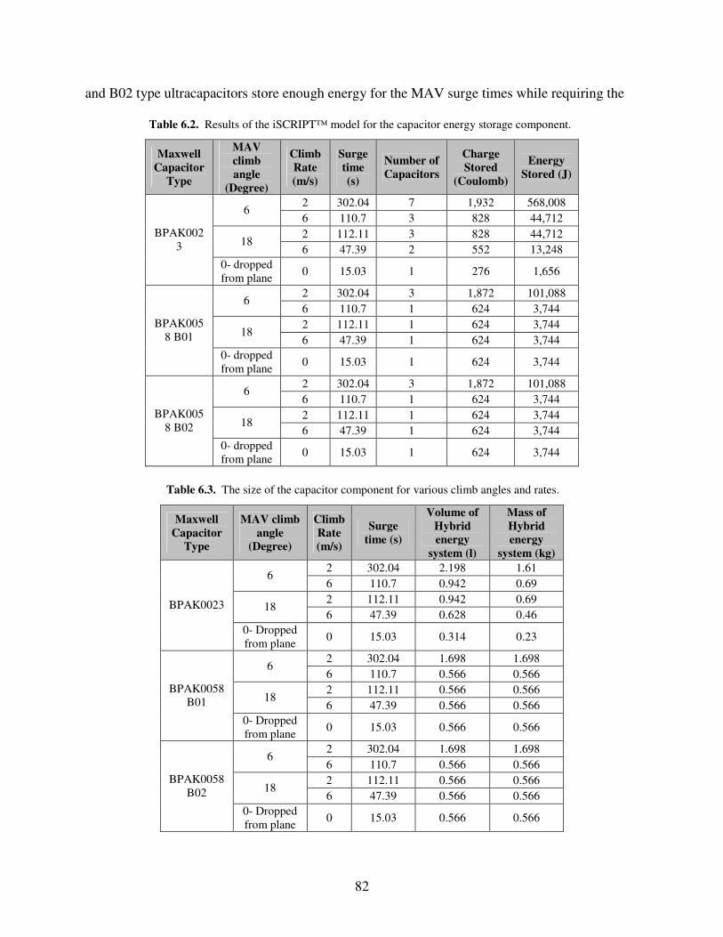
82

and B02 type ultracapacitors store enough energy for the MAV surge times while requiring the

Table 6.2. Results of the iSCRIPT™ model for the capacitor energy storage component.

Maxwell Capacitor

Type

MAV climb angle

(Degree)

Climb Rate (m/s)

Surge time (s)

Number of Capacitors

Charge Stored

(Coulomb)

Energy Stored (J)

2 302.04 7 1,932 568,008 6

6 110.7 3 828 44,712 2 112.11 3 828 44,712

18 6 47.39 2 552 13,248

BPAK0023

0- dropped from plane 0 15.03 1 276 1,656

2 302.04 3 1,872 101,088 6

6 110.7 1 624 3,744 2 112.11 1 624 3,744

18 6 47.39 1 624 3,744

BPAK0058 B01

0- dropped from plane 0 15.03 1 624 3,744

2 302.04 3 1,872 101,088 6

6 110.7 1 624 3,744 2 112.11 1 624 3,744

18 6 47.39 1 624 3,744

BPAK0058 B02

0- dropped from plane 0 15.03 1 624 3,744

Table 6.3. The size of the capacitor component for various climb angles and rates.

Maxwell

Capacitor Type

MAV climb angle

(Degree)

Climb Rate (m/s)

Surge time (s)

Volume of Hybrid energy

system (l)

Mass of Hybrid energy

system (kg) 2 302.04 2.198 1.61

6 6 110.7 0.942 0.69 2 112.11 0.942 0.69

18 6 47.39 0.628 0.46

BPAK0023

0- Dropped from plane 0 15.03 0.314 0.23

2 302.04 1.698 1.698 6

6 110.7 0.566 0.566 2 112.11 0.566 0.566

18 6 47.39 0.566 0.566

BPAK0058 B01

0- Dropped from plane 0 15.03 0.566 0.566

2 302.04 1.698 1.698 6

6 110.7 0.566 0.566 2 112.11 0.566 0.566

18 6 47.39 0.566 0.566

BPAK0058 B02

0- Dropped from plane 0 15.03 0.566 0.566

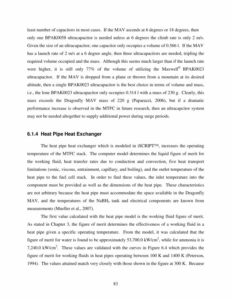
83

least number of capacitors in most cases. If the MAV ascends at 6 degrees or 18 degrees, then

only one BPAK0058 ultracapacitor is needed unless at 6 degrees the climb rate is only 2 m/s.

Given the size of an ultracapacitor, one capacitor only occupies a volume of 0.566 l. If the MAV

has a launch rate of 2 m/s at a 6 degree angle, then three ultracapacitors are needed, tripling the

required volume occupied and the mass. Although this seems much larger than if the launch rate

were higher, it is still only 77% of the volume of utilizing the Maxwell® BPAK0023

ultracapacitor. If the MAV is dropped from a plane or thrown from a mountain at its desired

altitude, then a single BPAK0023 ultracapacitor is the best choice in terms of volume and mass,

i.e., the lone BPAK0023 ultracapacitor only occupies 0.314 l with a mass of 230 g. Clearly, this

mass exceeds the Dragonfly MAV mass of 220 g (Paparazzi, 2006), but if a dramatic

performance increase is observed in the MTFC in future research, then an ultracapcitor system

may not be needed altogether to supply additional power during surge periods.

6.1.4 Heat Pipe Heat Exchanger

The heat pipe heat exchanger which is modeled in iSCRIPT™, increases the operating

temperature of the MTFC stack. The computer model determines the liquid figure of merit for

the working fluid, heat transfer rates due to conduction and convection, five heat transport

limitations (sonic, viscous, entrainment, capillary, and boiling), and the outlet temperature of the

heat pipe to the fuel cell stack. In order to find these values, the inlet temperature into the

component must be provided as well as the dimensions of the heat pipe. These characteristics

are not arbitrary because the heat pipe must accommodate the space available in the Dragonfly

MAV, and the temperatures of the NaBH4 tank and electrical components are known from

measurements (Mueller et al., 2007).

The first value calculated with the heat pipe model is the working fluid figure of merit.

As stated in Chapter 3, the figure of merit determines the effectiveness of a working fluid in a

heat pipe given a specific operating temperature. From the model, it was calculated that the

figure of merit for water is found to be approximately 53,700.0 kW/cm2, while for ammonia it is

7,240.0 kW/cm2. These values are validated with the curves in Figure 6.4 which provides the

figure of merit for working fluids in heat pipes operating between 100 K and 1400 K (Peterson,

1994). The values attained match very closely with those shown in the figure at 300 K. Because

84

water has the higher figure of merit in the operating temperature region around 300 K, it is the

more effective working fluid for the heat pipe being implemented into the MAV’ s fuel cell

system.

Figure 6.4. Figure of merit for common working fluids over a broad temperature range (Peterson, 1994; used with

permission by John Wiley & Sons, Inc.). The dimensions of the heat pipe heat exchanger must fit inside the MAV assumed here,

which has a length of 26 cm and a wingspan of 30 cm (Mueller et al., 2007). Figure 6.5 presents

a SolidWorks™ model of the Dragonfly MAV, which shows the NaBH4 tank next to the camera

and roughly in the center of the vehicle. The heat pipe’ s length must be small enough to fit

inside this MAV while being long enough to touch both the heat source (NaBH4 and electronics)

and sink (MTFC stack). A rough approximation of 10 cm is chosen as the length of the heat

pipe, and is only chosen as an assumed length through visual observation of Figure 6.5. The

radius of the heat pipe is chosen to be 2 cm for the model, which is a third the height of the

MAV’ s body (Mueller et al., 2007).

The temperature exiting the heat pipe is calculated with the computer model given an

inlet temperature into the heat pipe through an outer conductive layer from a thermal energy

source (e.g., the hydrogen storage tank and the camera). The exiting temperature values of the

heat pipe generated from the iSCRIPT™ model are provided in Table 6.4. The computer model

was only run with water as the working fluid, since it has the higher figure of merit. The table

85

presents the exiting temperature for a thermal energy source temperature between 50° C and 80°

C, which is the temperature range of the source. From this table, it is evident that a heat pipe with

Figure 6.5. SolidWorks™ model presenting a schematic of the Dragonfly MAV (Mueller et al., 2007; used with

permission of Dr. S.V. Shkarayev). copper walls, a copper conductive outer layer, and a wicking layer of either sintered copper or

nickel 100 mesh works the best for this application. By using these materials to fabricate the

heat pipe, the temperature difference between the two ends of the device is minimized,

maximizing the temperature of the fuel cell stack. For example, given a thermal energy source

temperature of 343 K (70° C), the outlet temperature going to the fuel cell stack is 336.9 K

(63.74° C) for a copper-water heat pipe. This is a temperature difference of 6.25 K. A typical

simple copper-water heat pipe has a temperature difference of 6° C, validating the model results

produced here (Peterson, 1994).

Figure 6.6 illustrates the temperature profile produced from the computer simulation

down the length of the heat pipe at important interfaces. This is in the predicted temperature

profile if the thermal energy source is at 343.15 K (70° C) and the heat pipe is a copper-water

device with a copper conductive outer layer. The figure shows profiles for all possible wicking

materials. A large temperature drop through the interior of the heat pipe is expected considering

that the working fluid thermal conductivities are much lower than for metals. The outlet

temperature of the heat pipe is always at its maximum when copper is used as the conductive

outer layer or wall material, regardless of the wick material.

The heat pipe computer model also calculates the five heat transport limitations and the

energy transferred through the device. If the energy transfer exceeds a specific limitation, then

86

Table 6.4. Modeled heat pipe entering and exiting temperatures for various working fluids and building materials.

Working Fluid Water

Wicking Material Nickel Felt Heat Pipe Wall

Material Lead Stainless Steel

Conductive Outer Layer Lead

Stainless Steel Aluminum Copper Lead

Stainless Steel Aluminum Copper

Entering Temperature

323.15 310.0 311.3 315.3 315.7 310.0 311.4 315.4 315.8 333.15 320.3 321.6 325.6 326.0 320.5 321.7 325.7 326.1 343.15 330.6 332.0 336.0 336.4 330.7 332.1 336.1 336.5 353.15 341.1 342.5 346.5 346.9 341.2 342.6 347.0 347

Heat Pipe Wall Material Aluminum Copper

Conductive Outer Layer Lead

Stainless Steel Aluminum Copper Lead

Stainless Steel Aluminum Copper

Entering Temperature

323.15 310.3 311.7 315.6 316.0 310.3 311.7 315.6 316.1 333.15 320.6 322.0 325.9 326.4 320.6 322.0 326.0 326.4 343.15 331.0 332.4 336.3 336.8 331.0 332.4 336.3 336.8 353.15 341.4 342.8 346.8 347.2 341.5 342.8 346.8 347.3

Wicking Material Sintered Copper Heat Pipe Wall

Material Lead Stainless Steel

Conductive Outer Layer Lead

Stainless Steel Aluminum Copper Lead

Stainless Steel Aluminum Copper

Entering Temperature

323.15 310.1 311.4 315.4 315.8 310.2 311.53 315.5 315.9 333.15 320.4 321.8 325.7 326.1 320.5 321.84 325.8 326.2 343.15 330.8 332.1 336.1 336.5 330.9 332.22 336.2 336.6 353.15 341.2 342.6 346.6 347.0 341.3 346.68 346.7 347.1

Working Fluid Water Wicking Material Sintered Copper

Heat Pipe Wall Material Aluminum Copper

Conductive Outer Layer Lead

Stainless Steel Aluminum Copper Lead

Stainless Steel Aluminum Copper

Entering Temperature

323.15 310.4 311.8 315.7 316.2 310.4 311.8 315.8 316.2 333.15 320.7 322.1 326.1 326.5 320.8 322.1 326.1 326.5 343.15 331.1 332.5 336.4 3369 331.1 332.5 336.5 336.9 353.15 341.6 342.9 346.9 347.4 341.6 343.0 347.0 347.4

87

Working Fluid Water Wicking Material Nickel 100 Mesh

Heat Pipe Wall Material Lead Stainless Steel

Conductive Outer Layer Lead

Stainless Steel Aluminum Copper Lead

Stainless Steel Aluminum Copper

Entering Temperature

323.15 310.1 311.4 315.4 315.8 310.2 311.5 315.5 315.9 333.15 320.4 321.8 325.7 326.1 320.5 321.8 325.8 326.2 343.15 330.8 332.1 336.1 336.5 330.9 332.2 336.2 336.6 353.15 341.2 342.6 346.6 347.0 341.3 346.7 346.7 347.1

Heat Pipe Wall Material Aluminum Copper

Conductive Outer Layer Lead

Stainless Steel Aluminum Copper Lead

Stainless Steel Aluminum Copper

Entering Temperature

323.15 310.4 311.8 315.7 316.2 310.4 311.8 315.8 316.2 333.15 320.7 322.1 326.1 326.5 320.8 322.1 326.1 326.5 343.15 331.1 332.5 336.4 336.9 331.1 332.5 336.5 336.9 353.15 341.6 342.9 346.9 347.4 341.6 343.0 347.0 347.4

modifications must be made to certain characteristics of the heat pipe. Table 6.5 presents the

results obtained from the computer model for the limitations and their comparison with the

energy transfer through the heat pipe when the thermal energy source is both the NaBH4

hydrogen storage tank and the electrical components of the MAV. The heat pipe modeled is

comprised of the materials mentioned earlier, which optimize its performance. The heat pipe is,

thus, fabricated with copper walls and a copper outer conductive layer and uses water as the

working fluid. Its total length is 10 cm; with the condenser, adiabatic, and evaporator sections

each accounting for one third the length. Furthermore, its diameter is 2 cm, and it has a wick

thickness of 0.2 mm. The thickness used is that same as found in Dunn and Reay (1994).

Based on the heat pipe results for energy transport limitations, temperature difference

across the device, and the liquid figure of merit, conclusions can me made about the construction

of the heat pipe for this application. Table 6.5 shows that the only limit exceeded (highlighted in

yellow) is the capillary limit for nickel 100 mesh, which for this mesh is lower than the energy

transferred across the heat pipe. This means that, given all the other characteristics of the heat

pipe, the working fluid extracted from the condenser end of the heat pipe can not return back to

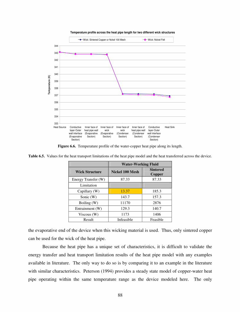
88

Temperature profile across the heat pipe length for two different wick structures

333

334

335

336

337

338

339

340

341

342

343

344

Heat Source Conductivelayer-Outer

wall interface(Evaporative

Section)

Inner face ofheat pipe wall(Evaporative

Section)

Inner face ofwick

(EvaporativeSection)

Inner face ofwick

(CondenserSection)

Inner face ofheat pipe wall(Condenser

Section)

Conductivelayer-Outer

wall interface(Condenser

Section)

Heat Sink

Tem

pera

ture

(K)

Wick: Sintered Copper or Nckel 100 Mesh Wick: Nickel Felt

Figure 6.6. Temperature profile of the water-copper heat pipe along its length.

Table 6.5. Values for the heat transport limitations of the heat pipe model and the heat transferred across the device.

Water-Working Fluid

Wick Structure Nickel 100 Mesh Sintered Copper

Energy Transfer (W) 87.33 87.33 Limitation

Capillary (W) 13.37 185.3 Sonic (W) 143.7 157.3

Boiling (W) 11170 2876 Entrainment (W) 129.3 140.7

Viscous (W) 1173 1406 Result Infeasible Feasible

the evaporative end of the device when this wicking material is used. Thus, only sintered copper

can be used for the wick of the heat pipe.

Because the heat pipe has a unique set of characteristics, it is difficult to validate the

energy transfer and heat transport limitation results of the heat pipe model with any examples

available in literature. The only way to do so is by comparing it to an example in the literature

with similar characteristics. Peterson (1994) provides a steady state model of copper-water heat

pipe operating within the same temperature range as the device modeled here. The only

89

differences are the wick structure and the size of the heat pipe. The iSCRIPT™ model

developed here is validated if the sonic and viscous limit values are in or near the range provided

by Peterson’ s example. The entrainment, boiling, and capillary limit can not be used for

validation since these values rely on the characteristics of the wick structure. In Peterson’ s

example, the sonic limit is between 48.85 W and 344.8 W, which is consistent with the results

generated here. The viscous limit of 1406 W in Table 6.5 also lies within the range provided by

Peterson’ s example, which ranges 219.3 W to 2095 W.

6.1.5 Fuel Cell Stack

The final component modeled here is the MTFC stack. This iSCRIPT™ model is based

on the one for MTFCs developed by Richard Evans (2007), which, he produces polarization

curves for MTFCs given certain environmental and fabrication conditions. The current model

expands upon this and quantifies how many MTFCs are needed in the fuel cell stack for various

operating temperatures and given cell characteristics. For example, Figure 6.7 shows the model

predictions for the number of MTFCs needed in the stack for three operating temperatures. The

power output of the fuel cell stack is 24 W and each cell operates at 0.5 v and a varying current

between 0.9 and 1.5 A. Each cell has an active surface area of 7.2 cm2. The RH for the

hydrogen anode gas is 75% and for the air cathode gas (requiring a small amount of desiccant to

lower the RH to this), 90%. The anode gas has a flow rate of 100 sccm, and the cathode flow

rate of 3000 sccm. The later is calculated based on fuel cells fabricated for experimentation at

Virginia Tech and volumetric flow rates used on them in the past. MTFCs with this active

surface area will be placed in the prototype structure. Table B.2 in Appendix B presents more

results quantifying the number of MTFCs needed in the stack at other loads, but the same

operating conditions of flow and RH. The results in Appendix B are for an operating

temperature of 343.15 K (70° C). As can be seen from this figure, if the stack operates at, for

example 325 K (52° C), then 40 MTFCs as designed for the prototype structure provides enough

power for the MAV during its cruise segments. This also requires, however, that the thermal

energy source for the heat pipe be at 333.15 K (60° C).

RH also plays a key role in determining the MTFC quantity in the fuel cell stack

component. A number of polarization curves are produced from the model at various RHs

90

between 50% and 100%. The operating conditions used to generate these curves are the same as

the previous model simulation determining the quantity of cells required at different

temperatures, with the exception of cathode gas RH (which is varied), and operating temperature.

The operating temperature used to generate this model is 343.15 K (70° C).

0

10

20

30

40

50

60Number of cells

Amount of fuel cells needed for several operating temperatures

T= 300 K T= 325 K T=350 K

Figure 6.7. Illustration of the number of Nafion® TT-060 prototype length MTFCs required for the stack at varying

temperatures to achieve a 24 W power output for the MAV.

From the preceding modeling results, conclusions can be made with respect to operating

conditions are needed to reduce the number of cells required for the fuel cell stack. Thus, for

example, to have 40 MTFCs or less in the stack (i.e., number in the prototype currently), the

operating temperature must be at least 52° C, the current density of each cell greater than 0.1

A/cm2, and the RH of the cathode air between 50% and 100%. These results also dictate that the

thermal energy source for the copper-water heat pipe should be at a temperature of at least 60° C

and that any amount and type of desiccant not exceeding one gram should suffice.

91

Polarization Curve R e lative to a Change in R H for an M TFC

0.00

0.20

0.40

0.60

0.80

1.00

1.20

0.00 0.20 0.40 0.60 0.80 1.00 1.20 1.40 1.60 1.80

J (A/cm ^ 2)

E (V

)

50% 60% 70% 80% 90% 100%

Figure 6.8. Polarization curves calculated for various air RHs.

6.2 Experimental Results

The experimental results for this section were obtained using the methods and testing

procedures described in Chapter 4. These results are used to gauge what fabrication methods and

materials should be used to create the best performing MTFCs. Some of the MTFC MEAs tested

were prepared by Luna Innovations, Inc., and others by the Center for Energy Systems Research

at Virginia Tech. Over 200 MTFC MEAs were prepared during this research project, and the

final MTFCs produced from the MEAs resulted in several hundred polarization, electrochemical

impedance spectroscopy, and lifetime tests. Due to the large volume of data produced, only the

best results will be presented in this thesis. Additional results and figures can be found in

Appendix C and in the monthly reports produced for Luna Innovations by Virginia Tech. Given

this data, a set of precise instructions is created for MTFC fabrication. The MTFC and catalyst

ink fabrication steps can be found in (preparations not included due to ITAR restrictions).

92

6.2.1 Best Performing Fuel Cells

From all the tests run, the five best performing cells were VT 11, made by Virginia Tech,

FCF 105-A, FCF 107-A, FCF 130, and FCF 115-A, which were made by Luna Innovations, Inc.

The appended letter to the number indicates that the original test conducted for the MTFC were

altered in some way and the original MTFCs tested again. Descriptions of the operational

conditions and operational changes are given in Table 6.6. Table 6.7 presents the characteristics

of these MTFCs and their performance values.

Table 6.6. Description of operational changes made to run the best performing MTFCs.

FCF # Original Operational Condition Operational Changes

VT11 100 sccm hydrogen none

VT11-A 100 sccm hydrogen reduction of anode flow rate to 75 sccm hydrogen

105-A Open to ambient air at room RH (~48%)

change from ambient air RH to 100%RH cathode air in test flask

107-A Open to ambient air at room RH (~48%)

change from open to ambient air to 100 sccm 100% RH hydrogen, 3000

sccm 100% RH air

VT11-D 100 sccm hydrogen reduction of anode floe rate to 25 sccm hydrogen

Table 6.7. Performance values for the four best fuel cells made during this research, including data attained when

they were modified.

Cell

Active Area (cm2)

Anode Conduction

Layer

Cathode Conduction

Layer Max Eoc Max PD

Min Real Impedance

VT #11 3.13 Gold Wire

Gold Wire and Nano-Fiber

Carbon Wrap 0.77 1.00E+00 1.05

VT #11-A 3.13 Gold Wire

Gold Wire and Nano-Fiber

Carbon Wrap 0.78 9.80E-01 1.64

FCF #105-A 2.76 Gold Wire

Gold Wire and Nano-Fiber

Carbon Wrap 0.78 9.36E-01 1.28

FCF #107-A 2.75 Gold Wire

Gold Wire and Nano-Fiber

Carbon Wrap 0.68 9.18E-01 1.28

VT #11-D 3.13 Gold Wire

Gold Wire and Nano-Fiber

Carbon Wrap 0.79 9.13E-01 1.38

FCF #130 3.41 Gold Wire

Gold Wire and Nano-Fiber

Carbon Wrap 0.71 9.11E-01 1.77

93

As can be seen from Table 6.7, the best performing MTFC is VT #11, having a maximum

power density of 1.00, a minimum real impedance of 1.05, and maximum open circuit voltage of

0.77. This cell was fabricated at Virginia Tech and the fact that it performed much better than

any other cells made at Luna proves that MTFC construction detail is not only important when

making MTFCs, but that it is perhaps the most vital factor that affects the cell performance.

6.2.2 Fuel Cells Made by Luna Innovations, Inc.

The MTFCs labeled as FCFs were prepared by Luna Innovations. The studies of these

cells conducted were for the purpose of finding the best fabrication conditions and materials, as

explained in Chapter 4. The purpose of these studies was to determine what Nafion® type to use

when preparing the MTFC. The different Nafion® types considered here are TT-030, TT-050,

TT-060, TT-070, and TT-110. Figure 6.9 shows the performance characteristics of the two most

promising, TT-050 and TT-060. Of these, Nafion® TT-050 performs the best with a higher

average power density and lower average high-frequency as shown in Figure 6.9. However

Table 6.8 shows otherwise, with average performance values being the highest with TT-060.

Although the cells should hypothetically be fabricated from Nafion® TT-050 given the model

results, they will use TT-060 instead because the material is more resistant to crossover, and all

testing done on FCFs favorably point to its use.

Additional studies were conducted on the Luna MTFCs aimed at determining the best

mixture for the MTFC catalyst ink to use to create the anode and cathode layers. All of these

studies were conducted in the same operating conditions, with 100 sccm hydrogen being

supplied as the humid anode gas, and 3000 sccm air being supplied as the cathode gas to a

humidity chamber. Some of these studies focused on integrating different percentages of

materials into the catalyst layer. One such material is called E-fill, which is a nickel-based

conductive powder that could improve the conductivity of the anode and cathode catalyst layers.

E-fill powder replaces a carbon nano-fiber (CNF) powder which performs the same task. Three

cells made by Luna Innovations with E-fill were tested twice, once with a gold wire and once

with a gold wire and Thornel™ carbon nano-fiber wrap conduction layer on the cathode side of

each individual MTFC. The conduction layer on the anode side of the MTFC is gold plated

copper wiring coiled inside the cell. Carbon fiber wrap was almost always used in the fuel cells

94

as a way to enhance the collection of electrons on the cathode side of the MTFCs. Table 6.9

presents data for the E-fill study. The designation “ A” designates a trial when both carbon nano-

fiber wrap and gold wire were used for the cathode conduction layers.

Table 6.8. Average performance values for the Luna fuel cells fabricated with different Nafion® types.

OCV Max PD PD @ 0.5V

High Frequency Impedance

TT-030 0.73 5.17E-02 4.32E-02 103.79 TT-050 0.58 2.57E-01 2.91E-01 5.64 TT-060 0.69 3.47E-01 3.56E-01 3.82 TT-070 0.70 5.59E-02 5.48E-02 51.03 TT-110 0.63 1.55E-01 1.46E-01 23.95

P olariz ation C urve R elative to N afion Type

0.00

0.20

0.40

0.60

0.80

1.00

1.20

0.00 0.50 1.00 1.50 2.00J (A/cm^2)

E (V

)

0

0.1

0.2

0.3

0.4

0.5

0.6

0.7

PD

(W/c

m2)

TT-050 C urrent Dens ity TT-060 C urrent D ens ityPD C urve TT-060 PD Curve TT-050

Figure 6.9. Modeled polarization curve for MTFC with TT-050 and TT-060 type Nafion®.

The following FCFs were tested with various amounts of E-fill in their catalyst layer ink:

• 3% E-fill, not CNF: FCF 159

• 7% E-fill, not CNF: FCF 158

• 10% E-fill, not CNF: FCF 157

Of the cells made with E-fill in the catalyst layer, FCF 158 containing 7% E-fill performed the

best with the highest maximum power density, OCV, and lowest impedance. These percentages

represent the proportion of E-fill present within the ink mixture by mass. It can be concluded

that, if E-fill were to be used in place of the pyrograph vapor grown carbon nano-fiber

95

(PyVGCF) in the catalyst ink, the powder should be 7% by mass of the ink. However, the

performance values presented for all fuel cells using E-fill in the catalyst are not as good as the

top performing cells prepared with PyVGCF in the catalyst layer instead. Therefore, it was

decided not to use E-fill in the ink formulation for the catalyst layer. Additionally, E-fill is not

Table 6.9. Performance values for Luna made fuel cells incorporating E-fill in the catalyst layer.

FCF # % E-fill in place of CNF

Relative Humidity

(%)

Max Power Density

Power Density at

0.5 v OCV

High Frequency Impedance

157 10 89 3.81E-01 2.79E-01 0.56 18.97 157-A 10 90 6.29E-02 N/A 0.31 17.69

158 7 87 7.45E-01 7.32E-01 0.74 14.36 158-A 7 87 6.14E-01 6.69E-01 0.74 14.62

159 3 81 2.12E-02 1.23E-02 0.64 21.28 159-A 3 84 1.71E-02 6.19E-03 0.48 14.36

used because of the nickel present in the powder and Nafion®’ s high affinity for their protons

may damage the MTFC. More information about this phenomenon is presented in a later

section.

The next question to ask is how much PyVGCF should be introduced into the catalyst

ink. In the PyVGCF study of cells prepared by Luna Innovations, the weight percentage of the

PyVGCF powder was varied from 1% to 7% in order to determine which percentage produces

the highest performing MTFC. Table 6.10 presents data from this study. Note that seven

percent represents the maximum possible mass that can be introduced into the catalyst layer

because any greater amount may result in catalyst ink clumping and ink blockage in the MTFC.

From the study, there does not seem to be a clear trend between performance and the amount of

PyVGCF added to the catalyst ink. The study does indicate that adding too much PyVGCF

powder results in a significant decrease in power density. Based on these results, it was decided

that 4% to 5% PyVGCF powder would suffice for the catalyst ink formula, since these

percentages lead to the highest power density or open circuit voltage.

Another study conducted was that for the mass percentage of platinum powder used in

the catalyst. The mass percentages are 10%, 20%, and 40% platinum in the catalyst ink. To

make the effect of platinum loading equal, the 10% solution was coated on the cell four times,

the 20% twice, and the 40% only once. Table 6.11 presents results from this study and shows

96

that 20% wt platinum catalyst ink coated twice on the MTFC has the maximum performance.

The cell using this formulation has the highest power density and the lowest impedance.

Table 6.10. PyVGCF study results.

FCF # % PyVGCF

Max Power Density

OCV High Freq. Impedance

82-A 1 2.91E-01 0.67 5.20 83-A 2 1.71E+01 0.66 5.76 84-A 3 3.08E-01 0.65 10.17 75-A 4 3.36E-01 0.84 7.31 85-A 5 6.33E-01 0.68 4.29 93-A 6 2.10E-01 0.69 3.72 94-A 7 1.72E-01 0.62 5.19

Table 6.11. Results from the platinum study with various platinum loadings.

FCF # % Platinum

Max Power Density OCV High Freq.

Impedance Coated #

times

134 10 5.06E-01 0.68 2.20 4 136 20 7.85E-01 0.76 1.89 2 137 40 2.81E-01 0.79 2.49 1

The catalyst ink to be applied must also be sonicated in order to break up colloidal

suspension of particles in the ink. The duration of this step is the subject of one study. The

sonication periods tested for this study are 1 min, 2 min, 4 min, and 8 min. Table 6.12 presents

the results. Luna’ s FCF 141 achieved the highest power density and second lowest high-

frequency impedance. Although the OCV is not as high as for the other cells in this study, the

power density is somewhat higher than that for the others when the ink sonication time is 2 min.

Although this study was not conclusive, it was determined that an intermediate sonication time

of, for example, two minutes is the best to use.

Table 6.12. Results of the sonication study on four Luna prepared fuel cells.

FCF # Sonication Time (min)

Sonication Wattage

Max Power Density OCV High Freq.

Impedance

140 1 9 5.35E-01 0.74 2.39 141 2 9 7.47E-01 0.72 1.66 142 4 9 5.97E-01 0.76 1.61 143 8 9 4.32E-01 0.75 4.22

97

When the catalyst ink is applied to the inside and outside of a micro-tubular membrane to

form an MEA, it is baked for an hour and at a certain temperature. To determine the ideal

processing temperature for MEA, a temperature study was conducted on two Luna prepared

MEAs, labeled FCF 160 and 161. They were fabricated to replace FCF 151 and 152, which had

very low maximum power densities and high impedances. The two micro-tubular MEAs were

prepared with baking temperatures of 170° C and 200° C. FCF 160 was baked at 170° C, and

161 at 200° C. The results for this study are shown in Table 6.13. Note that all the MEAs were

made of Nafion® TT-060 and a 4% PyVGCF catalyst ink. Based on the results shown in Table

6.13, FCF 144, baked at the lower temperature of 150° C, performed better than 160 at 170° C

and FCF 161 baked at 200° C. The implication is that the lower bake temperature is not only

better but may, in fact, point to some upper limitation temperature above which rapid

degradation of material occurs resulting in significantly worse performance.

Table 6.13. Temperature study results for MTFCs processed at 150° C, 170° C, and 200°C.

FCF # Process

Temperature (°C)

Max Power Density OCV High Freq.

Impedance

144 150 4.80E-01 0.81 2.38 160 170 2.43E-03 0.40 22.26 161 200 1.44E-01 0.78 7.05

In addition to bake temperature, a blowout study was conducted with the purpose of

finding a proper way to apply catalyst to the anode side of the MTFC. The anode interior is

difficult to coat uniformly and can only be coated using a needle and syringe. Blowout simply

refers to the volumetric flow rate of catalyst ink flowing into the MTFC to coat its anode interior.

The four blow out rates tested were 2.5 l/min, 5 l/min, 10 l/min, and 20 l/min. This is done using

a flow controller and sensors which can regulate flows as low as 13 ml/min. Table 6.14 presents

the performance results of this study. They seem to indicate that the rate at which catalyst ink is

applied to the anode side of the micro-tubular membrane should not exceed 10 l/min, since at

higher flow rates, the catalyst ink flows through the MTFC too fast resulting in insufficient

coverage and a loss in performance. The results for rates less than or equal to 10 l/min are

inconclusive.

The studies presented above, combined with research done on catalyst ink formulations

reported in the literature, lead to a number of conclusions regarding the catalyst ink mixture, its

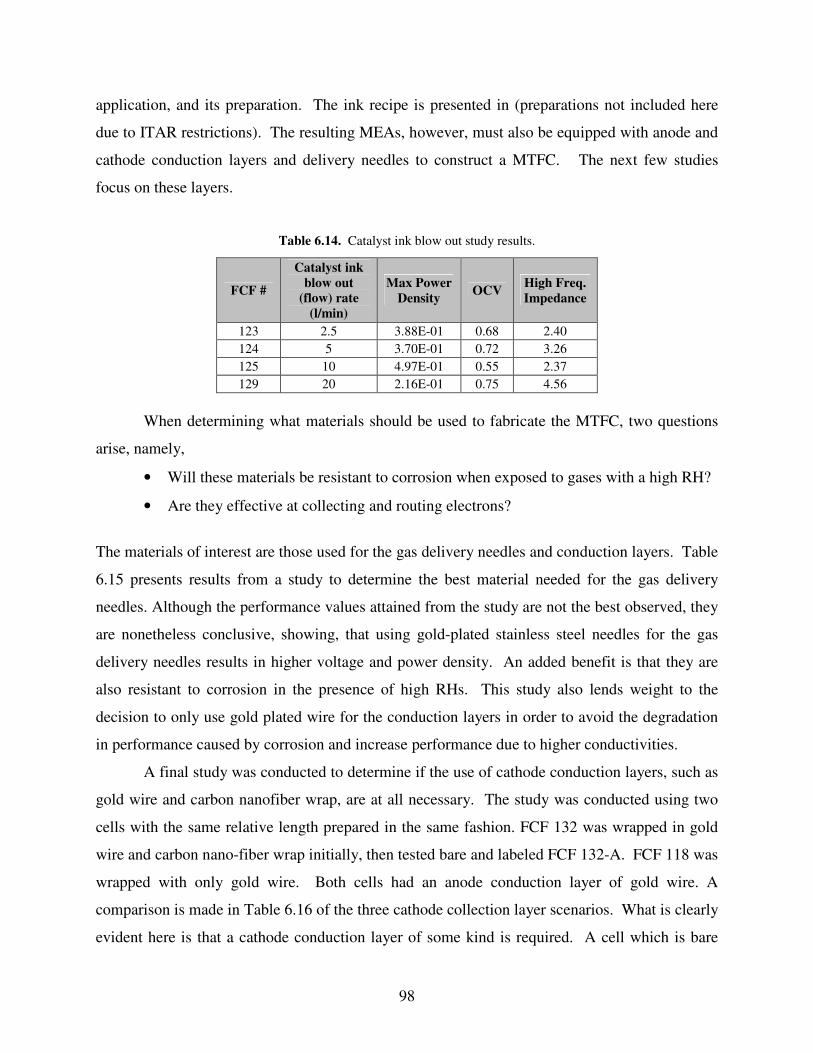
98

application, and its preparation. The ink recipe is presented in (preparations not included here

due to ITAR restrictions). The resulting MEAs, however, must also be equipped with anode and

cathode conduction layers and delivery needles to construct a MTFC. The next few studies

focus on these layers.

Table 6.14. Catalyst ink blow out study results.

FCF #

Catalyst ink blow out

(flow) rate (l/min)

Max Power Density OCV High Freq.

Impedance

123 2.5 3.88E-01 0.68 2.40 124 5 3.70E-01 0.72 3.26 125 10 4.97E-01 0.55 2.37 129 20 2.16E-01 0.75 4.56

When determining what materials should be used to fabricate the MTFC, two questions

arise, namely,

• Will these materials be resistant to corrosion when exposed to gases with a high RH?

• Are they effective at collecting and routing electrons?

The materials of interest are those used for the gas delivery needles and conduction layers. Table

6.15 presents results from a study to determine the best material needed for the gas delivery

needles. Although the performance values attained from the study are not the best observed, they

are nonetheless conclusive, showing, that using gold-plated stainless steel needles for the gas

delivery needles results in higher voltage and power density. An added benefit is that they are

also resistant to corrosion in the presence of high RHs. This study also lends weight to the

decision to only use gold plated wire for the conduction layers in order to avoid the degradation

in performance caused by corrosion and increase performance due to higher conductivities.

A final study was conducted to determine if the use of cathode conduction layers, such as

gold wire and carbon nanofiber wrap, are at all necessary. The study was conducted using two

cells with the same relative length prepared in the same fashion. FCF 132 was wrapped in gold

wire and carbon nano-fiber wrap initially, then tested bare and labeled FCF 132-A. FCF 118 was

wrapped with only gold wire. Both cells had an anode conduction layer of gold wire. A

comparison is made in Table 6.16 of the three cathode collection layer scenarios. What is clearly

evident here is that a cathode conduction layer of some kind is required. A cell which is bare

99

does not perform as well as one with such a layer and has an impedance several times higher. As

to be expected, FCF 132 with gold wire and carbon nano-fiber wrap had the best performance

with a power density higher than FCF 118 and FCF 132-A. Based on this study, it was

concluded that each cell be wrapped in gold wire and carbon nano-fiber wrap.

Table 6.15. Needle type study results.

FCF #

Gas delivery Needle Type

Max Power Density OCV High Freq.

Impedance

139 Plastic 3.49E-01 0.75 3.87 148 Steel 3.69E-01 0.53 1.72

154 Stainess Steel 5.40E-01 0.62 1.34

Table 6.16. Cathode collection layer study results.

FCF # Cathode Collection Layer Max

Power Density

OCV High Freq. Impedance

118 Gold Wire 1.72E-01 0.72 7.22 132 Gold Wire and Carbon Nanofiber 7.87E-01 0.68 1.79

132-A Bare 4.85E-02 0.64 15.77

6.3 Prototype MTFCs

Using the procedures developed from the studies above, MTFCs were made for

implementation into the MTFC stack prototype. After the cells were fabricated, each MTFC was

tested individually on the Fuel Cell Technologies test stand to determine whether it could be

utilized in the prototype. Although a few of them were labeled FCF like those prepared by Luna,

the majority of the cells were given the designation PR followed by a number. The only cells

with FCF designation were FCF 173 to 176. In addition, there were also labels such as renamed

PRH, PRW, PRX, PRY, and PRZ, depending on how those cells were prepared differently than

regular PR cells. For example, PRH 01 is a cell reheated during preparation in an inert nitrogen

environment at 150° C, which was not part of the original preparation scheme for prototype

MTFCs. The primary reason why this was done was because of poor performance values

observed when the original PR cells were tested. An explanation for the poor performance

values observed for the PR cells is discussed in a later section. The initial results from testing

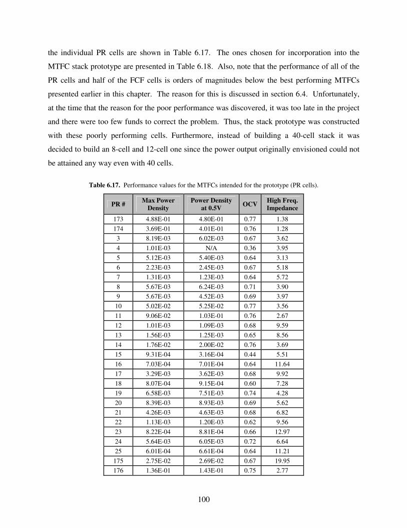
100

the individual PR cells are shown in Table 6.17. The ones chosen for incorporation into the

MTFC stack prototype are presented in Table 6.18. Also, note that the performance of all of the

PR cells and half of the FCF cells is orders of magnitudes below the best performing MTFCs

presented earlier in this chapter. The reason for this is discussed in section 6.4. Unfortunately,

at the time that the reason for the poor performance was discovered, it was too late in the project

and there were too few funds to correct the problem. Thus, the stack prototype was constructed

with these poorly performing cells. Furthermore, instead of building a 40-cell stack it was

decided to build an 8-cell and 12-cell one since the power output originally envisioned could not

be attained any way even with 40 cells.

Table 6.17. Performance values for the MTFCs intended for the prototype (PR cells).

PR # Max Power Density

Power Density at 0.5V OCV High Freq.

Impedance

173 4.88E-01 4.80E-01 0.77 1.38 174 3.69E-01 4.01E-01 0.76 1.28

3 8.19E-03 6.02E-03 0.67 3.62 4 1.01E-03 N/A 0.36 3.95 5 5.12E-03 5.40E-03 0.64 3.13 6 2.23E-03 2.45E-03 0.67 5.18 7 1.31E-03 1.23E-03 0.64 5.72 8 5.67E-03 6.24E-03 0.71 3.90 9 5.67E-03 4.52E-03 0.69 3.97

10 5.02E-02 5.25E-02 0.77 3.56 11 9.06E-02 1.03E-01 0.76 2.67 12 1.01E-03 1.09E-03 0.68 9.59 13 1.56E-03 1.25E-03 0.65 8.56 14 1.76E-02 2.00E-02 0.76 3.69 15 9.31E-04 3.16E-04 0.44 5.51 16 7.03E-04 7.01E-04 0.64 11.64 17 3.29E-03 3.62E-03 0.68 9.92 18 8.07E-04 9.15E-04 0.60 7.28 19 6.58E-03 7.51E-03 0.74 4.28 20 8.39E-03 8.93E-03 0.69 5.62 21 4.26E-03 4.63E-03 0.68 6.82 22 1.13E-03 1.20E-03 0.62 9.56 23 8.22E-04 8.81E-04 0.66 12.97 24 5.64E-03 6.05E-03 0.72 6.64 25 6.01E-04 6.61E-04 0.64 11.21

175 2.75E-02 2.69E-02 0.67 19.95 176 1.36E-01 1.43E-01 0.75 2.77

101

In addition to testing the prototype MTFCs individually, a few were also tested in series

and parallel. PR 8 and PR 9 were tested in series and parallel as a way to validate their electrical

integrity. This experiment was also conducted to attain a glimpse at what should be expected

when 40 fuel cells are placed in a stack. As expected, the voltage and resistance added in series

Table 6.18. MTFCs used in three prototype structure setups for testing.

Prototype 01

Cells Prototype 02

Cells Prototype 03

Cells PRY 04 PRY 04 PRZ 11 PRY 06 PRY 06 PRZ 12 PRZ 05 PRZ 05 PRZ 14 FCF 176 FCF 176 PRZ 07 PRZ 10 PRZ 10 PRY 01 PRY 05 PRZ 03 PRZ 13 PRZ 06 PRZ 06 PRX 01 PRY 07 PRY 07 PR 27

PRZ 01 PRY 03 PRZ 02 PR 10

and did not in parallel, while the power density remained relatively the same. Table 6.19

presents the results of the series and parallel tests of PR 08 and 09. Because resistances in series

are higher than expected, the power density is lower. This was observed for other PR cells as

well so modifications were made to these MTFCs to improve their performance before

implementation into the prototype. Although these modifications did improve cell performance,

it did not optimize them to values observed from previously prepared FCF cells by Luna. As

mentioned above, the reason why the PR cells performed so poorly is explained in a following

section.

Table 6.19. Prototype cell orientation test results.

PR # Orientation Max Power Density

Power Density at 1/2 OCV OCV High Freq.

Impedance

8 & 9 Series 3.48E-03 3.67E-03 0.73 4.04 8 & 9 Parallel 7.43E-03 6.15E-03 0.70 2.67

102

The modifications made to the prototype MTFCs processing or other operating

conditions varied. One modification was the heating conditions of the MTFC prior to use. A

cell was heated in inert nitrogen at 150° C before it was tested. This trial is referred to as PRH

01. In addition, the cell was soaked in deionized water overnight in order to hydrate the MTFC

membrane (PRW 01). The cathode flow rate was also altered to 200 sccm for one modification;

and for another, the cathode gas was supplied completely dry (both denoted PRX 01). Their

results are presented in Table 6.20. The results indicate that power density and open circuit

voltage are highest when the cathode flow is higher volumetrically. Considering that air is

supplied to the fuel cell stack in the MAV passively, this can be accomplished relatively easily

by passing as air through the stack due to the vehicle’ s motion as it flies at a velocity of about 50

kph.

Table 6.20. Prototype cells modification study results.

PR # Modification Max

Power Density

Power Density at 1/2 OCV

OCV High Freq. Impedance

PRH 01 Reheated for one hour in 150° C inert Nitrogen environment before testing 3.57E-03 3.95E-03 0.73 5.37

PRW 01 Soaked in DI H2O overnight 2.71E-03 2.20E-03 0.64 3.94 PRX 01 200 SCCM cathode flow rate 9.89E-02 4.14E-02 0.75 N/A

PRX 01 0% RH anode hydrogen flow (AKA dry) 1.37E-02 7.67E-03 0.60 5.19

The MTFC stack prototype was tested by flowing hydrogen through the stack at 100

sccm and with a high relatively high RH near 80%. Two cathode gas flow channels enter into a

chamber, of which the prototype is inside, at 3000 sccm. Both anode and cathode gas leave the

test station to enter the prototype at roughly room temperature. These conditions were applied

for testing of the prototype structure every time, unless otherwise noted. These conditions are

the test conditions for testing whose results are displayed in Figures 6.10 to 6.22. When the

prototype MTFCs are dead ended, the flow rate of hydrogen reduces to prevent a blowout of the

stack. The OCV test for the prototype lasted 12 min and displayed a maximum voltage of 0.42,

as can be seen in Figure 6.10. For the prototype testing, 12 MTFCs were placed into the

prototype stack to sample performance values. Given the data attained from the OCV test, the

MTFC prototype should produce enough voltage with only 25 MTFCs in the stack.

103

Three test sets were conducted on the prototype, two using 8 MTFCs, and another with

12 MTFCs. Results from the tests are presented graphically in Figure 6.11 through 6.18.

Figures 6.11 and 6.12 present lifetime tests for prototype 01 and prototype 02 using 8 cells as

mentioned previously. The lifetime tests were both conducted over a 30 minute span, the first

with a cathode RH of 48% and the second a RH of 100%. As is evidenced here, prototype 01

P rototype 03 Open C ircuit V oltage12 cells, 100 sccm anode gas, 48 % RH cathode

0.00E + 00

1.00E -01

2.00E -01

3.00E -01

4.00E -01

5.00E -01

0.00E+ 00

1.00E+ 02

2.00E+ 02

3.00E+02

4.00E+ 02

5.00E+ 02

6.00E+ 02

7.00E+02

8.00E+ 02

Tim e (se c)

OC

V

Figure 6.10. Open circuit voltage test results over a 12-minute time span.

P rototype 01 Life tim e Te stLong P R c ells , quantity 8, gold wire and CNF wrap c athode collec tion

layer, m edium RH of 48%

0.00E + 00

5.00E -04

1.00E -03

1.50E -03

2.00E -03

2.50E -03

3.00E -03

3.50E -03

4.00E -03

0.00 5.00 10.00 15.00 20.00 25.00 30.00

Tim e (m in)

Pow

er D

ensi

ty

Figure 6.11. Lifetime test of the first trial of the MTFC prototype.

104

lifetime test generally did not perform as well as prototype 02’ s lifetime test in terms of power

density. Over the course of the lifetime test, the power density of prototype 02 dropped and then

started to recover after 15 minutes. The lifetime test of prototype 01 did not recover at all, due to

a drying out of the membrane and lower cathode gas RH.

Figure 6.13 presents the lifetime test conducted on prototype 03, the third prototype test

P rototype 02 Life tim e Te stGold wire and CNF wrap cathode c ollec tion lay er, 8 long cells in the

prototy pe, 100% RH anode gas

0.00E + 001.00E -042.00E -04

3.00E -044.00E -045.00E -046.00E -047.00E -04

8.00E -049.00E -041.00E -03

0.00 5.00 10.00 15.00 20.00 25.00 30.00

Tim e (m in)

Pow

er D

ensi

ty

Figure 6.12. Second trial of the MTFC stack prototype lifetime test with 8 MTFCs.

Figure 6.13. Lifetime test of the MTFC stack prototype with 12 MTFCs in the stack.

105

series conducted with 12 MTFCs installed into the prototype structure. This test was also

conducted for a period of 30 min. When 12 cells were placed in a stack, the initial power density

was higher by nearly an order of magnitude, and leveled off its performance after 10 min. The

increased performance is not correlated with MTFC quantity necessarily, but that the additional

four added cells had higher power densities individually than the original 8 PR MTFCs. Figure

6.14 presents results from a polarization test conducted on the 8-cell prototype 01 test series.

Figure 6.15 is a polarization curve of the other 8-MTFC arrangement. When run with a

100% RH cathode gas flow, the maximum power density observed is over three times that of

prototype 01 with a lower RH cathode flow, as to be expected. The prototypes are not heated but

left at room temperature. Prototype 03 is run under different conditions than prototype 02 or 01.

For this test series, 12 MTFCs are laid flat and delivered hydrogen gas through a universal gas

flow tube is applied to all 12 cells. This test scenario is discussed in the second section of

Chapter 5 and the testing conditions detailed in Table 6.21.

Prototype 01 Pola riz a tion CurveLong Cells , quantity 8, gold wire and CNF wrap cathode collec tion layer,

m edium RH of 48%

0.000

0.500

1.000

1.500

2.000

2.500

3.000

3.500

0.00E +00

2.00E -05

4.00E -05

6.00E -05

8.00E -05

1.00E -04

1.20E -04

1.40E-04

1.60E -04

I(A/cm ^ 2)

E

0.00E+ 00

5.00E-04

1.00E-03

1.50E-03

2.00E-03

2.50E-03

3.00E-03

P

Figure 6.14. First potentiodynamic (polarization) test of the 8-cell MTFC stack prototype.

Figure 6.16 presents the polarization curve results for prototype 03. It shows a higher

power density than the previous polarization curves but is not impressive given the values seen

for the best performing MTFCs. The lack of a sound curve in this figure and the previous figures

does indicate that there could be a problem with the cells. A non-stable curve may indicate a

buildup of water in the anode or an elevated and non-uniform high-frequency impedance of the

106

cells. Figure 6.17 presents results from an EIS test conducted on prototype 02. Figure 6.18

presents similar results for an EIS of prototype 03.

The first EIS trial of prototype 01 with 8 cells in the stack is done with air at a 48% RH

and results in real impedances between 500 and 1025. In addition, the EIS test has an erratic

Prototype 02 Pola riz a tion CurveGold wire and CNF wrap c athode c ollec tion layer, fuel cell s tac k prototype, 8

cells , 100% RH anode gas

0.000

0.100

0.200

0.300

0.400

0.500

0.600

0.700

0.00E+ 00 5.00E -05 1.00E-04 1.50E -04 2.00E -04 2.50E -04I(A/cm ^ 2)

E

0.00E + 00

2.00E -04

4.00E -04

6.00E -04

8.00E -04

1.00E -03

1.20E -03

1.40E -03

1.60E -03

P

Figure 6.15. Second potentiodynamic (polarization) test of the 8-cell MTFC stack prototype.

P rototype 03 P ola riza tion CurveGold wire and CNF wrap cathode c ollec tion lay er, 12 c ells , high RH anode

gas

0.0000.100

0.2000.3000.400

0.5000.600

0.7000.800

0.00E +00 5.00E -05 1.00E-04 1.50E -04 2.00E -04 2.50E -04 3.00E -04I(A/cm ^2)

E

0.00E +00

2.00E -03

4.00E -03

6.00E -03

8.00E -03

1.00E -02

1.20E -02

1.40E -02P

Figure 6.16. Potentiodynamic test of the 12-cell MTFC stackprototype.

behavior, with a zigzag curve that had ranges from a few � to several hundred � in real

impedance. It should be noted that for every EIS tests for the prototype were assigned the same

107

specific settings prior to testing. The frequency set for all prototype EIS tests is 100 kHz. The

DC voltage for the EIS test was set at ½ the voltage observed for the whole stack in the

polarization curve. EIS tests for prototype 02 and 03 are much more promising and have lower

P rototype 02 EIS Gold wire and CNF wrap cathode collec tion layer, fuel cell

s tack of 8 cells , 100% RH anode gas flow

0.00

5.00

10.00

15.00

20.00

25.00

30.00

0 5 10 15 20 25

Z'(a ) (re a l im pe de nce )

-Z''(

b) (i

mag

inar

y im

pede

nce)

Figure 6.17. Second EIS of the 8-cell MTFC stack prototype.

high-frequency impedances. A detailed discussion explaining why prototype 01 has bad

impedance values is discussed in the next section. However, the principal cause is that

P rototype 03 EIS Gold wire and CNF wrap cathode collec tion layer, 12 cells

in s tack , high RH

0.00

5.00

10.00

15.00

20.00

25.00

30.00

35.00

0 5 10 15

Z'(a ) (re a l im pe de nce )

-Z''(

b) (i

mag

inar

y im

pede

nce)

Figure 6.18. Electrochemical impedance spectroscopy of the 12-cell MTFC stack prototype.

108

membranes of the PR cells are contaminated with metal cations resulting in a moisture loss in the

Nafion®. Increasing the relative humidity of the air surrounding the MTFCs introduces water

back into the polymer membranes, allowing the cells to restore their conductivity to some extent.

Once water is introduced into the membrane to offset the displaced water eliminated from the

contamination effect, the cell resistances decrease. These tests show the performance of the

prototype when equipped with 8 and 12 fuel cells. The lifetime tests of both trials indicate that

the power stays relatively constant, albeit low, over time. This fact, along with the conclusion

made from the polarization test that power increases with an increase of fuel cell quantity, is

promising for the fuel cell stack in the MAV. The impedance is lower and more stable when the

hydrogen gas RH is high, which is expected given that the Nafion® membrane should ideally be

wet.

The prototype is also tested with the MTFCs dead-ended, meaning that a controlled flow

of hydrogen travels through the cells, which are blocked at their ends. This is the basis of the

original design of the MTFC stack prototype, which has the fuel cells dead-ended. However, due

to a lack of a pressure regulator within the hydrogen entry tank of the prototype design, an exit

hydrogen enclosure is created instead. Figures 6.19 to 6.22 present the results from testing the

prototype with dead-ended MTFCs. These tests are done with 12 MTFCs in the stack and a

moderate RH of 54% for the air. A second EIS was done with 12 dead-ended MTFCs but with a

cathode air RH of 75%. For all these tests, the operating conditions are as shown in Table 6.21.

Table 6.21. Operating conditions for the prototype tests ran.

Prototype 01

Prototype 02

Prototype 03

Prototype 03- dead

ended

Prototype 03- dead ended, 2nd trial

RH anode gas 100% 100% 100% 100% 100% RH cathode gas 48% 48% 54% 54% 75% Anode flow rate 100 sccm 100 sccm 100 sccm <<100 sccm <<100 sccm

Cathode flow rate open air open air open air open air open air

Operating temperature 25-28° C 25-28° C 25-28° C 25-28° C 25-28° C

Cells in stack 8 8 12 8 8

Figure 6.19 presents the results from a lifetime test of the prototype when 12 MTFCs are

dead-ended for a thirty min duration, and a cathode RH of 54%. The power density quickly

109

dropped after two minutes and leveled of without any recovery whatsoever for the remaining 28

min. Figure 6.20 presents results from a polarization curve conducted on the dead-ended cells,

P rototype 03 Life tim e Te stGold wire and CNF Cathode c ollec tion layer, 12 tubular fuel c ells , RH

54% cathode gas , high anode gas RH, dead ended

0.00E + 00

5.00E -04

1.00E -03

1.50E -03

2.00E -03

2.50E -03

3.00E -03

0.00 5.00 10.00 15.00 20.00 25.00 30.00

Tim e (m in)

Pow

er D

ensi

ty

Figure 6.19. Lifetime test of the MTFC stack prototype with 12 MTFCs in the stack dead-ended.

Prototype 03 Pola riz a tion CurveGold wire and CNF wrap c athode collec tion layer, 12 cells in s tack , 54% RH

cathode gas , high RH anode gas , dead ended cells

0.0000.1000.2000.3000.4000.5000.6000.7000.800

0.00E+ 00

2.00E-05

4.00E -05

6.00E -05

8.00E -05

1.00E -04

1.20E -04

1.40E -04

1.60E -04

1.80E -04

I(A/cm ^2)

E

0.00E + 001.00E -042.00E -043.00E -044.00E -045.00E -046.00E -047.00E -048.00E -049.00E -04

P

Figure 6.20. Polarization test of the MTFC stack prototype with 12 dead-ended MTFCs in the stack.

which proves that the prototype cells have poor performance due to the erratic behavior of the

curve (as mentioned earlier).

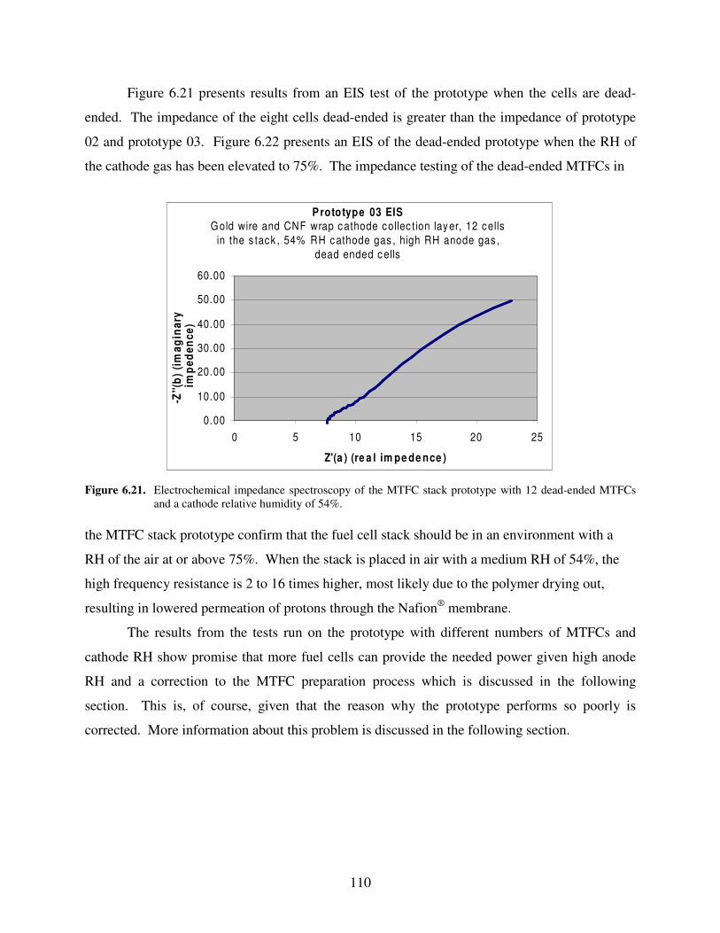
110

Figure 6.21 presents results from an EIS test of the prototype when the cells are dead-

ended. The impedance of the eight cells dead-ended is greater than the impedance of prototype

02 and prototype 03. Figure 6.22 presents an EIS of the dead-ended prototype when the RH of

the cathode gas has been elevated to 75%. The impedance testing of the dead-ended MTFCs in

P rototype 03 EIS

Gold wire and CNF wrap cathode collec tion layer, 12 cells in the s tack , 54% RH cathode gas , high RH anode gas ,

dead ended cells

0.00

10.00

20.00

30.00

40.00

50.00

60.00

0 5 10 15 20 25

Z'(a ) (re a l im pe de nce )

-Z''(

b) (i

mag

inar

y im

pede

nce)

Figure 6.21. Electrochemical impedance spectroscopy of the MTFC stack prototype with 12 dead-ended MTFCs

and a cathode relative humidity of 54%. the MTFC stack prototype confirm that the fuel cell stack should be in an environment with a

RH of the air at or above 75%. When the stack is placed in air with a medium RH of 54%, the

high frequency resistance is 2 to 16 times higher, most likely due to the polymer drying out,

resulting in lowered permeation of protons through the Nafion® membrane.

The results from the tests run on the prototype with different numbers of MTFCs and

cathode RH show promise that more fuel cells can provide the needed power given high anode

RH and a correction to the MTFC preparation process which is discussed in the following

section. This is, of course, given that the reason why the prototype performs so poorly is

corrected. More information about this problem is discussed in the following section.

111

P rototype 03 EIS Gold wire and CNF wrap cathode collec tion layer, 12 cells in series , 75% RH cathode gas , high RH anode gas , dead

ended cells

0.002.004.006.008.00

10.0012.0014.0016.0018.0020.00

0 2 4 6 8 10

Z'(a ) (re a l im pe de nce )

-Z''(

b) (i

mag

inar

y im

pede

nce)

Figure 6.22. Electrochemical impedance spectroscopy of the MTFC stack prototype with 8 dead-ended MTFCs in

75% RH cathode environment.

6.4 Reasons for the MTFC Stack Prototype’s Performance

The poor performance of the MTFC stack prototype and the low testing polarization and

high EIS values can be attributed to metal ion leaching of the gold anode collection wire,

contaminating the Nafion® polymer membrane of the MTFC. When the fuel cells are prepared

for the stack prototype, they already have gold anode wiring inside them when they are placed

into a sulfuric acid bath to be acid converted. Normally, soaking the gold plated wire in sulfuric

acid would not affect it because the gold coating is thick enough to withstand the acidic effect for

a few hours. Unfortunately, when the prototype cells were fabricated towards the end of the

project, a cheaper gold wire was used than what was previously employed to make the FCF and

VT series of MTFCs. The wire used for the prototype cells was 34 gage, having a gold (Au)

coating layer 0.0004 in (0.0010 cm) thick. When MTFCs were fabricated previously, 32 gage

wires were used, having a gold coating 0.0005 in (0.0013 cm) thick on the exterior. A difference

of 0.0001 in (0.00030 cm) of gold coating was enough to allow acid penetration of the Au

surface and cationic leaching of copper and gold to occur. This was evidenced by the sulfuric

acid turning blue in color after 20 of the PR cells were soaked in the liquid for an hour. When

metallic components are placed in a clear liquid and the liquid becomes discolored to a blue hue,

112

this suggests that copper ions have leached out of the components and are suspended in the

liquid. The first two prototype cells, FCF 173 and 174 were not affected by the effect of copper

cation contamination of the cell membranes because only those two cells were placed into the

acid bath, not 20. When a large number of cells (i.e., 20) are placed together in an acid bath,

enough copper ions are leached out of the anode collection wires to significantly influence the

polymer membrane walls of the cell, contaminating the Nafion®. The contamination of PEM

polymer membranes from metal ions, like copper, damages the conductivity and durability of the

fuel cell.

Nafion® is damaged significantly by metal ions primarily because of the polymer’ s

affinity for their charge. A copper ion is defined chemically as Cu2+, indicating that it has a

charge of +2, twice that of a hydrogen proton (H+). As discussed previously, Nafion®’ s

electronegative sulfonic acid group tail has an affinity to a positive charge that is very strong and

gets stronger with increased charge. Thus, Nafion®’s affinity to copper ions is greater than its

affinity to hydrogen protons. In terms of Nafion®’ s affinity to various ions, the following

inequality holds:

Fe3+>Ni2+>Cu2+>H+ (6.1)

This means that any leached metallic ion carrying more charge bonds to the polymer’ s sulfonic

acid groups instead of the hydrogen proton. When metallic cations bond to the Nafion® transport

sites, they displace hydrogen protons and expel water molecules with them. Water is expelled

from the Nafion® membrane because the displacing metallic ions are heavier than the hydrogen

protons, and sulfonate salt is formed whenever sulfuric acid sites bond to the copper cations.

The introduction of salt into a polymer causes the membrane to shrivel and lose moisture.

Displacement of hydrogen ions and a loss of water result in a drastic drop in cell conductivity

and an increase in resistance (St-Pierre et al., 2000). Figure 6.23 is a chemical schematic of

Nafion® contamination as a result of bathing too many MTFCs in sulfuric acid. The high

impedance values presented in Table 6.17 indicates that the conductivity dropped significantly

due to this metallic contamination effect. Had the prototype cells been bathed individually in

sulfuric acid or in small quantities, the poor MTFC performance observed during testing would

have been eliminated. This is noted in the preparation steps for the MTFC, guaranteeing that

113

next time a fuel cell stack prototype is made, the MTFC membranes will not be contaminated. In

addition, it should also be noted that gold wire gage 32 should be used in the MTFC preparation.

Figure 6.23. Chemical schematic of Nafion® copper ion contamination in the MTFC membrane.

114

7 Chapter Seven – Conclusions

The results of the iSCRIPT™ model of the MTFC stack system have been presented in

this thesis and indicate that the NaBH4 hydrogen storage tank with a volume roughly 3.0 in3 fits

within the fuselage of a MAV such as the Dragonfly with a fuselage volume of 4.65 in3 (Mueller

et al., 2007). However, more space is needed to accommodate the fuel cell stack, the

ultracapacitors used for surge energy storage, and the heat pipe used for thermal energy transfer

to the fuel cell stack. While the fuel cell stack prototype has a volume of 5.94 in3 and would fit

(at least on a volume basis though not necessarily on a dimensional basis) the heat pipe adds an

additional volume of 7.68 in3, and the capacitors 19.2 in3. The total volume for these last two

components is 26.8 in3, filling approximately half a liter. This is not large if implemented in a

slightly larger UAV (i.e., the Casper 250).

Although the size of the MTFC system is larger than desired, immense improvements

have been made to the performance of the MTFCs since the research endeavor began. The

power density of the MTFC has improved by 5000% over the course of this project due to

process changes in fuel cell preparation. In addition, compared to the best fuel cells tested in

2007 which had a maximum OCV of 0.826, OCVs exceeding 0.91 have been recorded in the

past year. Fuel cell high frequency impedances have also been lowered significantly due to

changes in MTFC preparation. In 2007, impedances were observed to range from 50 � to

10,000 �. Since then, the MTFC impedances have been reduced by several orders of magnitude

to values falling between 1 and 17.9. Even two cells when tested in series only had an

impedance of about 5.7; thanks to the new preparation method developed for the MTFCs from

modeling, experimentation, and directed trial and error.

When paired with the iSCRIPT™ model of the balance of the system, the iSCRIPT™

fuel cell stack designed provides enough power for the MAV throughout its entire mission.

Experimentation done on the MTFC stack prototype, although showing poor performance due to

copper ion contamination, did show that the stack was effective in at least providing some power

properly, given the design and cell configuration. However, more modifications and testing are

needed on the prototype to assure the complete success of the energy supply system. In addition,

the MTFC stack prototype and energy balance of system must be tested directly on an MAV in

order to truly gage what further modifications are necessary. The promising values attained from

115

the individual fuel cells when improvements were made to them by Virginia Tech and Luna

Innovations Inc, and the model of the system as a whole indicates that the designed fuel cell

stack, heat pipe, capacitor, and small chemical hydride tank could power a MAV if needed.

116

Copyright Permissions Figure 1.2. [used with permission]

EcoGeneration Solutions, LLC, 2002. http://www.cogeneration.net/carbonate_fuel_cells.htm

(accessed October 9, 2009) used with permission of M. Goodell; permission letter available.

Figure 1.3. [public domain]

U.S. Department of Energy. http://www1.eere.energy.gov/hydrogenandfuelcells/fc_anim

ation_components.html (accessed August 20, 2009)

Works by the U.S. Government are not eligible for copyright permission

Figure 1.4. [fair use]

DTI Energy, Inc., 2004, “ how Direct Methanol Fuel Cells (DMFC) work.”

http://www.dtienergy.com/process.html (accessed July 14, 2009); fair use determination

available.

Figure 2.1 [fair use]

Paparazzi, the Free Autopilot. User’ s Aircraft Gallery. http://paparazzi.enac.fr/wiki/Gallery

(accessed August 1, 2009); fair use determination available.

Figure 2.2. [used with permission]

Mueller, T.J., Kellogg, J.C., Ifju, P.G., Shkarayev, S.V., 2007. “ Introduction to the Design of

Fixed-Wing Micro Air Vehicles, Including Three Case Studies” , The American Institute of

Aeronautics and Astronautics, Inc, Reston, Virginia. Fig. 3.27, pp.144. used with permission of

Dr. S.V. Shkarayev; permission letter available.

Figure 2.3. [used with permission]

Defense Update, 2006, “ Casper 200/250 Miniature UAV” , http://defense-

update.com/products/c/casper200.htm (accessed January 14, 2009) used with permission of N.

Shental, CEO of Top I Vision; permission letter available.

Figure 2.4, Figure 2.5. [used with permission]

Coursange, J.-F., Hourri, A., and Hamelin, J., 2003, “ Performance Comparison Between Planar

and Tubular-Shaped PEM Fuel Cells by Three-Dimensional Numerical Simulation,” Fuel Cells,

Volume 3, Number 1-2, pp. 28-36, Copyright Wiley-VCH Verlag GmbH & Co. KGaA. Used

with permission of Dr. J. Hamelin; permission letter available.

117

Figure 2.7, Figure 2.8. [used with permission]

Coursange, J.-F., Hourri, A., and Hamelin, J., 2003, “ Performance Comparison Between Planar

and Tubular-Shaped PEM Fuel Cells by Three-Dimensional Numerical Simulation,” Fuel Cells,

Volume 3, Number 1-2, pp. 28-36, Copyright Wiley-VCH Verlag GmbH & Co. KGaA. Used

with permission of Dr. J. Hamelin; permission letter available.

Table 2.1. [used with permission]

Lund Instrument Engineering, inc., 2009, Powerstream Batteries and Battery Packs product

information page, http://www.powerstream.com/ (accessed August 30, 2009) reproduced with

permission of Dr. M.W. Lund; permission letter available

Figure 3.4. [used with permission]

Dick, S., Woynicki, J.T., 2002, “ Processing Technologies: Dealing with humidity” , IVD

Technology Magazine, June 2002 Issue, June 02, 2009, pp. 55, http://www.devicelink.com/

ivdt/archive/02/06/002.html (accessed June 1, 2009) used with permission of Canon

Communications, LLC; permission letter available.

Figure 3.5. [used with permission]

Chemical Engineers’ Resource, “ What is a Heat Pipe?,” http://www.cheresources.com/htpipes.sh

tml (accessed September 12, 2009) used with permission of S. Narayanan KR; permission letter

available.

Table 3.10. [used with permission]

Chemical Engineers’ Resource, “ What is a Heat Pipe?,” http://www.cheresources.com/htpipes.sh

tml (accessed September 12, 2009) used with permission of S. Narayanan KR; permission letter

available.

Figure 4.13. [used with permission]

Zhang, J., Tang, Y., Song, C., Xia, Z., Li, H., Wang, H., Zhang, J., 2008, “ PEM Fuel Cell

Relative Humidity (RH) and its Effect on Performance at High Temperatures” , Electrochimica

Acta 53 (2008), pp. 5315-5321. used with permission of Elsevier; permission letter available.

Figure 4.14. [used with permission]

Zhang, J., Tang, Y., Song, C., Xia, Z., Li, H., Wang, H., Zhang, J., 2008, “ PEM Fuel Cell

Relative Humidity (RH) and its Effect on Performance at High Temperatures” , Electrochimica

Acta 53 (2008), pp. 5315-5321 used with permission of Elsevier; permission letter available.

118

Figure 4.15 [used with permission]

Vaisala, 2009, Vaisala Humicap® Humidity and Temperature Transmitter Series HMT 330

product specification page, http://www.vaisala.com/instruments/products/hf-hmt330.html

(accessed September 11, 2009) used with permission of (courtesy of) Vaisala, Inc; permission

letter available.

Figure 6.4 [used with permission]

Peterson, G.P., 1994, “ An Introduction to Heat Pipes; Modeling, Testing, and Applications” ,

John Wiley and Sons, Inc., New York, New York, pp.212. used with permission of John Wiley

& Sons, Inc; permission letter available.

Figure 6.5 [used with permission]

Mueller, T.J., Kellogg, J.C., Ifju, P.G., Shkarayev, S.V., 2007. “ Introduction to the Design of

Fixed-Wing Micro Air Vehicles, Including Three Case Studies” , The American Institute of

Aeronautics and Astronautics, Inc, Reston, Virginia. Fig. 3.3, pp.117. used with permission of

Dr. S.V. Shkarayev; permission letter available.

119

References Al Baghdadi, M.A.R.S., 2008, “ Performance Comparison Between Planar and Tubular-

shaped Ambient Air-breathing Polymer Electrolyte Membrane Fuel Cells Using Three-

dimensional Computational Fluid Dynamics Models,” Journal of Renewable and Sustainable

Energy 1, 023105 (2009)

Antoine C., 1888, "Tensions des vapeurs; nouvelle relation entre les tensions et les

températures", Comptes Rendus des Séances de l'Académie des Sciences, 107, 681-684, 778-

780, 836-837

Arellano, J., 2006, “ Two Motorcycles that Joined the Alternative Power Movement” ,

autobloggreen.com, http://www.autobloggreen.com/tag/emissions+neutral+vehicle/

Asymtek, 2007, “ News extra: Catalyst ink is accurately dispensed on fuel cell

membranes” , Membrane Technology Journal, November 2007, pp 9

Brown, T.L., LeMay, H.E., Bursten, B.E., Burdge, J.R., 2003, “ Chemistry: The Central

Science” , 9th ed., Pearson Education, Inc., Upper Saddle River, New Jersey, pp 1046

Chandra, D., Reilly, J.J., and Chellappa, R., 2006, “ Metal Hydrides for Vehicular

Applications: The State of the Art,” Journal of Minerals, Metals, and Materials (JOM), TMS

(The Minerals, Metals, & Materials Society), February

Chemical Engineers’ Resource, 2008, “ What is a Heat Pipe?

http://www.cheresources.com/htpipes.shtml, accessed August 1, 2009

Coursange, J-F, Hourri, A., and Hamelin, J., 2003, “ Performance Comparison

between Planar and Tubular-Shaped PEM Fuel Cells by Three-Dimensional Numerical

Simulation,” Fuel Cells, Volume 3, Number 1-2, pp 28-36

Defense Update, 2006, “ Casper 200/250 Miniature UAV” , http://defense-

update.com/products/c/casper200.htm

Defense Update, 2009, “ Wasp III (BATMAV) Micro UAV” , http://defense-

update.com/products/w/wasp3.htm

Dick, S., Woynicki, J.T., 2002, “ Processing Technologies: Dealing with humidity” , IVD

Technology Magazine, June 2002 Issue, June 02, 2009, pp. 55, http://www.devicelink.com/

ivdt/archive/02/06/002.html, accessed June 1, 2009

120

DTI Energy, Inc, 2004, “ Direct Methanol Fuel Cell” ,

http://www.dtienergy.com/Resources/works.gif, accessed July 14, 2008

Dunn, P.D., Reay, D.A., 1994, “ Heat Pipes” , 4th ed., Pergamon Press, Tarrytown, New

York

Ecogeneration Solutions, LLC, 2002, “ Carbonate Fuel Cells” ,

http://www.cogeneration.net/carbonate_fuel_cells.htm

Eshragi, R.R., Lin, C., Lin, J.C., Ketterer, 2005, US Patent for Microfibrous Fuel

Cell Assemblies, Comprising Fiber-Supported Electrocatalyst Layers, and Methods of Making

Same, Patent # 20050151269, Date of Patent August 18, 2005, Assignee Microcell Corporation

Evans, R.B., 2007, “ Modeling and Testing of Micro-Tubular Low Temperature

Fuel Cell for Use in a Micro Air Vehicle” . Masters Thesis Submitted December 19, 2007.

Virginia Polytechnic Institute and State University

Gierke, T.D., Munn, G.E., Wilson, F.C., 1982, “ Perflourinated Ionomer Membranes” ,

American Chemical Society Symposium Series, Volume 180, Chapter 10, pp. 195-216

Gunter, J., 2007, “ Space Efficient Fuel Cell Fibers for Micro Air Vehicles (MAV),” U.S.

Air Force – Air Force Research Lab – Munitions Directorate –Eglin AFB Contract No. FA8651-

06-M-0192, Phase I Final Report

Ha, S., Larsen, R., Masel, R.I., 2005, “ Performance characterization of Pd/C nanocatalyst

for direct formic acid fuel cells,” Journal of Power Sources, 144, pp 28-34

J. St-Pierre, D. P. Wilkinson, S. Knights and M. Bos, 2000,“ Relationships between water

management, contamination and lifetime degradation in PEFC” , Ballard Power Systems, Burnay,

British Columbia, Journal of New Materials for Electrochemical Systems, Volume 3, pp. 99-106

Kimble, M.C., Anderson, E.B., Jane, K.D., Woodman, A.S., and Legner, H.H., 2000,

“ Electrochemical Performance of a Multi-Tubular Fuel Cell and Electrolyzer Array,”

Intersociety Energy Conversion Engineering Conference and Exhibit (IECEC), 35th, Las Vegas,

NV, July 24-28, 2000, Collection of Technical Papers. Vol. 1 (A00-37701 10-44)

Kojima, Yoshitsugu, 2005, “ Hydrogen Storage Generation Using Sodium Borohydride,”

R&D Review of Toyota CRDL Volume 40 No. 2, pp. 31-36

Larminie, J. and Dicks, A., 2003, “ Fuel Cell System Explained” , pp. 145, 148, and 149

Lin, J-L, Wei, C-Y, Lin, C-Y, 2007, “ Design and Testing of Fixed-Wing MAVs” ,

Emerald Publishing Group Limited, Taiwan

121

Liu, J.G., Zhao, T.S., Liang, Z.X., Chen, R., 2006, “ Effect of Membrane Thickness on

Performance and Efficiency of Passive Direct Methanol Fuel Cells” , Journal of Power Sources,

153, pp 61-67

Lund Instrument Engineering, inc., 2009, Powerstream Batteries and Battery Packs

product information page, http://www.powerstream.com/, accessed August 30, 2009

MAV Lab. University of Florida, 2007, “ UF MAV Lab Homepage” ,

http://mae.ufl.edu/mav/ accessed July 13, 2008.

Maxwell Technologies, 2009, Datasheet, 15 V Power and Series Ultracapacitor Packs,

http://www.maxwell.com/ultracapacitors/datasheets/DATASHEET_15V_series_1009361.pdf,

accessed February 16, 2009

Mench, M.M., Wang, Z.H., Bhatia, K., and Wang, C.Y., 2001, “ Design of a micro direct

methanol fuel cell (�DMFC),” International Mechanical Engineering Congress and Exposition

(IMECE), New York, New York, USA, November 11-16

Mueller, T.J., Kellogg, J.C., Ifju, P.G., Shkarayev, S.V., 2007, “ Introduction to

the Design of Fixed-Wing Micro Air Vehicles, Including Three Case Studies” , The American

Institute of Aeronautics and Astronautics, Inc, Reston, Virginia, pp 90,91, 80-88

O’ Hayre, R., Cha, S.W., Colella, W., and Prinz, F.B., 2006, “ Fuel Cell Fundamentals,”

John Wiley & Sons, Inc, Hoboken, New Jersey, pp 3-15, 39, 85, 239

Olson, D.H., Silin, D.H., Aki, M., Murrieta, C., Tyler, J., Kochevar, A., Jehle, A.,

Shkarayev, S., 2005 “ Wind Tunnel Testing and Design of Fixed and Flapping Wing Micro Air

Vehicles at The University of Arizona,” The University of Arizona

Osborn, S.J., Hassan, M.K., Divoux, G.M., Rhoades, D.W., Mauritz, K.A.,

Moore, R.A., 2007, “ Glass Transition Temperature of Perfluorosulfonic Acid Ionomers” ,

Macromolecules 2007, 40, pp 3886-3890

Paparazzi, the Free Autopilot, 2009, User’ s Aircraft Gallery, http://paparazzi.enac.fr/wiki

/Gallery, accessed August 1, 2009

Perma Pure LLC, 2007, Nafion® Tubing specifications

http://www.permapure.com/Products/NafionTubing.htm

Peterson, G.P., 1994, “ An Introduction to Heat Pipes; Modeling, Testing, and

Applications” , John Wiley and Sons, Inc., New York, New York, pp. 122-236, pp.212

122

Power One, 2006, power one product information for zinc-air batteries,

www.powerone-batteries.com

Steyn, W.J., 1996, United States Patent for Tubular Fuel Cell Assembly and Method of

Manufacture, Patent # 6007932, Date of Patent December 28, 1999 Assignee: Gore Enterprise

Holdings, Inc

St-Pierre, J., Wilkinson, D.P., Knights, S., and Bos, M., 2000, “ Relationships Between

Water Management, Contamination and Lifetime Degradation in PEFC” , Journal of New

Materials for Electrochemical Systems” , Volume 3, pp 99-106

Thunder Power Batteries, 2006, Thunder Power Batteries product information

www.thunderpower-batteries.com

Trulite Inc., 2009, “ Development of a 24 W-Hr Hydrogen Generator Cartridge for MAV

Application, Contract #: 1617-AFR-2S/Trulite”

US Department of Energy, 2008, Hydrogen, Fuel Cells, and Infrastructure Technologies

Program, “ Fuel Cell Components” , http://www1.eere.energy.gov/hydrogenan

dfuelcells/fc_animation_components.html

U.S. Department of Energy, 2008, “ Fuel Cell Technologies Program: Chemical

Hydrogen Storage,” http://www1.eere.energy.gov/hydrogenandfuelcells/storage/chem_storage.ht

ml

Vaisala, 2009, Vaisala Humicap® Humidity and Temperature Transmitter Series HMT

330 product specification page, http://www.vaisala.com/instruments/products/hf-hmt330.html,

accessed September 11, 2009

Wikimedia foundation Inc, 2008, “ Nafion®” . http://en.wikipedia.org/wiki/Nafion,

accessed July 15, 2008

Woodbank Communications, Ltd., 2005, Capacitors and Supercapacitor Electopaedia

resource page, http://www.mpoweruk.com/supercaps.htm, accessed March 17, 2009

Wu, Y., 2003, “ Hydrogen Storage via Sodium Borohydride- Current Status,

Barrier, and R&D Roadmap” , Millennium Cell, Inc, Eatontown, New Jersey, PowerPoint

presentation, http://gcep.stanford.edu/pdfs/hydrogen_workshop/Wu.pdf, accessed July 29, 2008

Yaws, C.L., Narasimhan, P.K., Gabbula, C., 2009, “ Yaws' Handbook of Antoine

Coefficients for Vapor Pressure (2nd Electronic Edition)” Knovel Publishing

Yeom, J., Mozsgai, G.Z., Flachsbort, B.R., Choban, E.R., Asthana, A., Shannon,

123

M.A., and Kenis, P.J.A., 2005, “ Microfabrication and Characterization of a Silicon-Based

Milimeter Scale PEM Fuel Cell Operating with Hydrogen, Methanol, or Formic Acid,” Sensors

and Actuators B Volume 107, pp 882-891

Zhang, J., Tang, Y., Song, C., Xia, Z., Li, H., Wang, H., Zhang, J., 2008, “ PEM Fuel Cell

Relative Humidity (RH) and its Effect on Performance at High Temperatures” , Electrochimica

Acta 53 (2008), pp. 5315-5321

124

Appendix A

Table A.1 presents the MTFC characteristics (cell structure, hardware, and catalyst ink

formulation and application) that were varied over the course of cell experimentation and studies.

Table A.1. Variations in MTFC characteristics which were tested throughout the project.

Characteristic Variation

Cell Structure TT-030 TT-050 TT-060 TT-070

Nafion® type TT-110 150°C 170°C 200°C 220°C

Process temperature 250°C Plastic Gold plated steel

Gas dispersion needle type Stainless steel Heat for 1 hr

Acid bath of fuel cell Leave in cold acid overnight Cell length 1.54 cm to 20.9 cm

Dry Storage method Deionized water

Catalyst ink formulation and application 1% 2% 3% 4% 5% 6%

PyVGCF (CNF) in ink by weight percent 7% PyVGCF only 3% E-fill only 7% E-fill only

E-fill to substitute PyVGCF, % wt. 10% E-fill only 1 min 2 min 4 min

Ink sonication time 8 min

125

Characteristic Variation Catalyst ink formulation and application

4 coats of 10% Pt 2 coats of 20% Pt

Platinum loading technique 1 coat of 40% Pt 2.5 l/min 5 l/min 10 l/min Volumetric flow rate of ink applied to the

anode 20 l/min Hardware

MWS® Wire Gold wire manufacturer California Fine Wire®

Bare Gold wire only Stainless steel wire Gold wire and CNF

Cathode collection layer CNF only

126

Appendix B

Table B.1 presents the results from the desiccant disc model simulation and the amount

of desiccant needed at a desired RH range from 10% to 100%. Although the mass of desiccant

needed to achieve higher relative humidities has a small difference between the three types, the

mass required for molecular sieve is much lower than the other two when the desired RH is

below 40%.

Table B.1. Model results for the amount of desiccant needed to adjust the hydrogen gas flow to specific RHs.

Desired

RH Amount Silica Gel Needed

(g) Amount Molecular Sieve

Needed (g) Amount Clay Needed

(g) 0.1 6.62 2.64 4.96 0.2 3.22 2.02 2.72 0.3 2.01 1.64 1.85 0.4 1.30 1.30 1.41 0.5 0.93 1.08 1.06 0.6 0.66 0.86 0.77 0.7 0.42 0.64 0.54 0.8 0.27 0.39 0.33 0.9 0.23 0.17 0.18 1 0 0 0

Table B.2 presents the model results for the MTFC fuel cell stack simulation which

provides the quantity of cells needed at an RH range from 50% to 100%. From the table, it is

clear that an increase in RH around the MTFC stack will result in a decrease of required cells to

meet the power of the MAV. In addition, as the current density increases, the required quantity

of MTFCs decreases.

Table B.2. Model results of the fuel cell stack presenting the quantity of cells required for the MAV. The cell

active area is that for the PR MTFCs.

Quantity of MTFCs

Active area of

cell=7.202 cm2

J (A/cm^2) RH 0.5 0.6 0.7 0.8 0.9 1 0.00 0 0 0 0 0 0 0.05 85 85 84 84 84 84 0.10 45 45 45 45 45 45 0.15 32 31 31 31 31 31 0.20 25 25 24 24 24 24 0.25 20 20 20 20 20 20

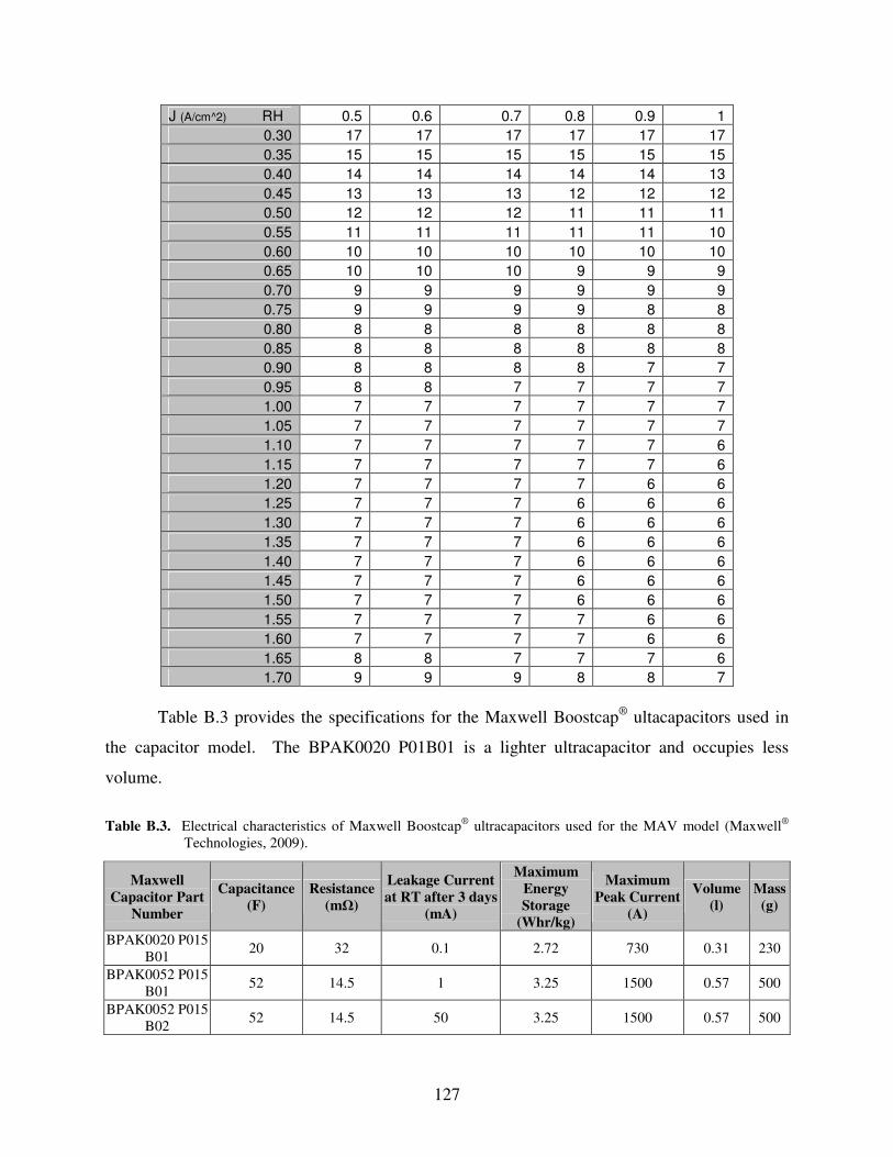
127

J (A/cm^2) RH 0.5 0.6 0.7 0.8 0.9 1 0.30 17 17 17 17 17 17 0.35 15 15 15 15 15 15 0.40 14 14 14 14 14 13 0.45 13 13 13 12 12 12 0.50 12 12 12 11 11 11 0.55 11 11 11 11 11 10 0.60 10 10 10 10 10 10 0.65 10 10 10 9 9 9 0.70 9 9 9 9 9 9 0.75 9 9 9 9 8 8 0.80 8 8 8 8 8 8 0.85 8 8 8 8 8 8 0.90 8 8 8 8 7 7 0.95 8 8 7 7 7 7 1.00 7 7 7 7 7 7 1.05 7 7 7 7 7 7 1.10 7 7 7 7 7 6 1.15 7 7 7 7 7 6 1.20 7 7 7 7 6 6 1.25 7 7 7 6 6 6 1.30 7 7 7 6 6 6 1.35 7 7 7 6 6 6 1.40 7 7 7 6 6 6 1.45 7 7 7 6 6 6 1.50 7 7 7 6 6 6 1.55 7 7 7 7 6 6 1.60 7 7 7 7 6 6 1.65 8 8 7 7 7 6 1.70 9 9 9 8 8 7

Table B.3 provides the specifications for the Maxwell Boostcap® ultacapacitors used in

the capacitor model. The BPAK0020 P01B01 is a lighter ultracapacitor and occupies less

volume.

Table B.3. Electrical characteristics of Maxwell Boostcap® ultracapacitors used for the MAV model (Maxwell®

Technologies, 2009).

Maxwell Capacitor Part

Number

Capacitance (F)

Resistance (m�)

Leakage Current at RT after 3 days

(mA)

Maximum Energy Storage

(Whr/kg)

Maximum Peak Current

(A)

Volume (l)

Mass (g)

BPAK0020 P015 B01 20 32 0.1 2.72 730 0.31 230

BPAK0052 P015 B01 52 14.5 1 3.25 1500 0.57 500

BPAK0052 P015 B02 52 14.5 50 3.25 1500 0.57 500

128

Appendix C Figure C.1 presents a polarization curve of VT 11, the best performing MTFC prepared

by Virginia Tech. Figure C.2 is a lifetime test of MTFC VT 11 conducted over a 30 min time

period in early 2009.

V T 11 P ola riz a tion Curve 100 sc cm 100% RH hy drgoen, 3000 sc cm 100% RH air

c arbon fiber & gold wrap

0.000

0.200

0.400

0.600

0.800

1.000

0.00E + 00

2.00E -02

4.00E -02

6.00E -02

8.00E -02

1.00E -01

1.20E -01

1.40E -01

I(A/cm ^ 2)

E

0.00E +00

2.00E -01

4.00E -01

6.00E -01

8.00E -01

1.00E +00

1.20E +00

P

Figure C.1. Polarization test curve of VT 11, the best performing MTFC ever made throughout the research.

V T 11 Life tim e Te st

100 scc m 100% RH hydrgoen, 3000 sc cm 100% RH aircarbon fiber & gold wrap

0.00E + 00

2.00E-01

4.00E-01

6.00E-01

8.00E-01

1.00E + 00

1.20E + 00

1.40E + 00

0.00 5.00 10.00 15.00 20.00 25.00 30.00

Tim e (m in)

Pow

er D

ensi

ty

Figure C.2. Lifetime test of VT 11, the best fabricated cell, over a 30 minute period.

129

Figure C.3 presents an electrochemical impedance spectroscopy (EIS) conducted for VT 11. In

this figure, the various loss regions are labeled to indicate where they occur.

The maximum current density observed during the lifetime test was over 1.10. Over the

lifetime test, the cell performance dropped with the applied load, and then recovered slightly

after 20 minutes. A cell that recovers during a 30 minute lifetime test is a promising sign that the

cell will perform well when placed in a stack and have a low high frequency impedance.

Figure C.3. Electrochemical impedance spectroscopy of VT 11 showing three distinct impedance loss regions

The EIS test conducted on VT 11 showed that this MTFC had one of the lowest

impedances of all cells tested at Virginia Tech. An EIS test graph of Figure C.3 is a Nyquist plot

illustrating where the loss effects occur. On VT 11, the cathode activation loss region is the

largest of the three, suggesting an increase resistivity on the cathode side of the MTFC.

Figure C.4 is a polarization curve conducted on FCF 105-A, the best MTFC prepared by

Luna Innovations to date, having a maximum power density of just below 1.0. Figure C.5

presents results from the EIS conducted on FCF 105-A. . The EIS test of FCF 105-A, done with

gold wire and carbon nanofiber wrap, illustrates a low real impedance of the MTFC. However,

unlike VT 11, the impedance increased more dramatically over the course of the test. This

suggests a cell which performs worse than VT 11. Given that VT 11 was fabricated at a Virginia

Tech laboratory and FCF 105-A was made at Luna Innovations, it can be assumed that a

difference in fabrication process led to a difference in cell membrane conductivity.

130

FCF 105-A P ola riz a tion Curve100 sc c m 100% RH hy drogen, anode - A u, c athode - CF + A u

0.0000.1000.2000.3000.4000.5000.6000.7000.8000.900

0.00E+ 00 3.00E -02 6.00E -02 9.00E -02 1.20E -01 1.50E-01

I(A/cm ^ 2)

E

0.00E + 001.00E -012.00E -013.00E -014.00E -015.00E -016.00E -017.00E -018.00E -019.00E -011.00E + 00

P

Figure C.4. Polarization curve of the best MTFC prepared by Luna Innovations and is a modification of FCF 105

by testing it in a 100% RH air environment

FCF 105-A EIS 100 s cc m 100% RH hy drogen, anode - A u, c athode - CF + A u

0.001.00

2.003.004.00

5.006.007.00

8.009.00

0 5 10 15 20

Z'(a ) (re a l im pe de nce )

-Z''(

b) (i

mag

inar

y im

pede

nce)

Figure C.5. Electrochemical impedance spectroscopy of FCF 105-A, the best MTFC prepared by Luna Innovations Figure C.6 presents the results of the polarization test conducted on MTFC FCF 107-A, a

good performing cell made by Luna Innovations. Figure C.7 presents the EIS results or FCF

107-A. The polarization curve for FCF 107-A is a cell which shows no inconsistencies or erratic

bumps. This is characteristic of a well-made cell which does not suffer from any flooding or ion

131

contamination at all. Similarly, the EIS of FCF 107-A is one that does not show any

inconsistencies.

FCF 107-A P ola riz a tion Curve150 sc cm 100% RH hy drogen, 3000 sc cm 100% RH air

c athode - CF + A u wrap

0.0000.1000.2000.3000.4000.5000.6000.7000.800

0.00E +00

2.00E -02

4.00E -02

6.00E-02

8.00E -02

1.00E -01

1.20E -01

1.40E -01

1.60E -01

I(A/cm ^ 2)

E

0.00E + 00

2.00E -01

4.00E -01

6.00E -01

8.00E -01

1.00E + 00

P

Figure C.6. Polarization curve of FCF 107-A, the second best performing Luna prepared fuel cell, placed in air at

an RH of 100%

FCF 107-A EIS 150 sccm 100% RH hydrogen, 3000 sccm 100% RH air

cathode - CF + A u wrap

0.00

0.05

0.10

0.15

0.20

0.25

0.30

0 1 2 3 4

Z'(a ) (re a l im pe de nce )

-Z''(

b) (i

mag

inar

y im

pede

nce)

Figure C.7. Electrochemical impedance spectroscopy (EIS) of FCF 107-A in 100% RH air.

132

Appendix D A bill of materials for the products used to make the prototype structure is presented in

Table D.1. In total, 73 parts will be needed to fabricate the prototype structure and MTFC stack.

Table D.1. Bill of materials for the fuel cell prototype

Item Part Number Unit

QTY QTY Material/ Source

1 hydrogentank_oneeightsinch 1 2 PTFE 2 o-ring 5 2 McMaster-Carr 3 small teflon plate 1 2 PTFE 4 Silicone Septum 1 2 Silicone 5 Big_PTFE_disc_oneeigthshole 1 2 PTFE

6 electriccollection_disc 1 1 Radio Shack PC Board

7 tubular_cell 1 40 Nafion® 8 seperation_plates_for_cells 1 2 PTFE 9 Long screws 1/8" thick & 11" length 4 4 McMaster-Carr

10 Short screws 1/8" thick & 0.375" length 4 8 McMaster-Carr 11 Bolts inner diameter 1/8" 12 8 McMaster-Carr

Table D.2 presents how Nafion® is prepared in tetrabutylammonium (TBA) in methanol prior to

being prepared as a fuel cell (Osborn et al., 2007). Details about this process were explained in

Chapter 2.

Table D.2. Procedure to prepare a Nafion® membrane in TBA in methanol.

Procedure Steps Step # Description

1 Clean the membrane in refluxing nitric acid (8 M) for 2 hours

2 Rinse the membrane three times in deionized water

3 Boil the membrane in deionized water for one hour

4 Perform partial neutralization by stirring the membranes with TBAOH/methanol solution for 12 hours with a stir bar

5 Boil the membrane in methanol for 1 hour

6 Dry the membrane in a vacuum oven overnight at 70°C

Tetrabutyl Ammonium Membrane Preparation

7 Rinse the membrane in deionized water