Modeling floods in Enxoé watershed

Student: Petre Ioana

Year: 2013

Modeling floods in Enxoé watershed

1

Abstract

Enxoé reservoir was built in 1998. Enxoé is a temporary river with tendency to flushy regime and

the flood dynamics, that may impact reservoir state, was characterized using the following approach:

Collect data in the, until then, ungauged watershed (2010-2011);

Implement MOHID Land model and validate the hydrology against existing data, and

With the model validated, quantify flood role on annual loads and depict flood dynamics.

It was observed that soil loss of permeability in Enxoé is an important factor to accurately predict

first floods or first peaks of consecutive floods and cumulative load results with orders similar to

urbanized watersheds reinforced this fact. First floods in the year had a lower weight in terms of annual

volume and annual nutrient load to the reservoir (less than 3% and 7% respectively) that floods in winter

(between 10%-20% each). However, first floods in the year transported particulates concentrations that

were 5 to 50 times the low waters value (and most of the transported occurred in the first minutes of flood,

before flow peak, from deposited material in river bed and in neighbor land areas), while in winter,

concentration remained almost constant during flood. Further work should link watershed models to a

reservoir model in order to depict the flood impact in the reservoir and test management strategies to

reduce trophic state. (David Brito, Ramiro Neves).

Modeling floods in Enxoé watershed

2

Acknowledgements

I would like to thank to Maretec team, to Professor Ramiro Neves, Mr. David Brito for their help,

for guiding our steps in MOHID Land and for their warmly receiving in their group.

This paper work is part of „EUTROPHOS Project” (PTDC/AGR-AAM/098100/2008) of the

Fundação para a Ciência e a Tecnologia (FCT) http://eutrophosproject.wordpress.com/.

Also I would like to thank to Mr. Frank Braunschweig, who gave me free license for Mohid Studio

program of Action Modulers Company, during the development of this work.

Modeling floods in Enxoé watershed

3

1st Chapter. Introduction

From a strict hydrological sense, flood is defined as a rise, usually brief, in the water level in a

stream to a peak from which the water level recedes at a slower rate (UNESCO-WMO 1974).

Flood is a natural phenomenon that occurs when the volume of water flowing in a system exceeds

its total water holding capacity.

The natural phenomenon can have several sources as: prolonged rain with considerable intensity,

dam or dike break, river blockages, storm surges.

In recent history, floods are becoming more frequent and severe and some organizations even

counted it as the most damaging natural disaster in a region. In Europe, flooding, is the most common

natural disaster and the most costly in economic terms. The Emergency Disasters Data Base (EM-DAT)

has recorded a total of 238 flood events in European region from 1975 to 2001.

The frequency of occurrence and the intensity of damages and losses of lives resulting from floods

made it known all over the world that flood is a great treat to humanity. However, since serious floods

occur in a certain location with a return period of years or decades, the lessons learned from previous

flood may have been forgotten (Miller, 1997).

The direct effects of floods includes: losses of lives, damage to property, disruption of

transportations, communications, health and community services, crop and livestock damages and

interruptions and losses in business.

The consequence of floods has called for the growing attention because of the need to prevent or

control flood damages in our society. Mitigating flood damages can be drawn in two possible ways:

structural measures and non-structural measures. Structural measures include the building of dikes, dams

and reservoirs and channel improvements designed to reduce the incidence or extent of flooding.

Structural mitigation measures are methods designed to divert flood water away from people. This type of

mitigation measures are proven effective but most often expensive.

The non – structural method of mitigating flood damages place people away from the flood.

The aim of this work was flood modeling in Enxoé watershed. The primary objectives of the

study are:

- To determine the flood behavior including design flood levels;

- To provide a model that can establish the effects on flood behavior of future development.

- To simulate watershed and reservoir dynamics and to represent the actual situation and test

management.

Modeling floods in Enxoé watershed

4

2nd

Chapter. Literature survey

2.1 Hydrologic cycle at catchment scale

At a catchment scale, considerations of hydrological cycle include the processes that take place in

the atmosphere, land surface and subsurface. The precipitation falls from the atmosphere but before it

reaches the ground, part of it is intercepted by vegetation and evaporates back into the atmosphere. The

precipitation that reaches the land surface will either infiltrate to the subsurface or will become Horton

overland flow or rill flow. As the rill flow accumulates, it becomes a stream flow then channel flow.

Channel flow also has some contribution from the groundwater flow in the form of baseflow; it becomes

the catchment runoff when it flows out from the catchment.

Rainwater that infiltrates will contribute to unsaturated flow, macro pore flow and perched flow.

Unsaturated flow will recharge the groundwater through the process of percolation. Water that passes

through macro pore and perched flow will either contribute to the groundwater flow or to the exfiltration

process depending on the soil moisture condition. When rainwater reaches the groundwater through

percolation, part of it will join the channel flow as baseflow and again evaporation will take place.

Majority of the groundwater will remain as groundwater recharge or groundwater storage. The total

evaporation is the summation of the canopy evaporation, transpiration and soil evaporation and

evaporation from open water. The catchment runoff is the accumulation of the channel flow and the

contribution from the groundwater.

2.2 Runoff processes

The concept that surface runoff is generated where and when the rainfall intensity exceeds the

rate at which water can enter the soil, most hydrologists considered that all storm runoff was generated by

this mechanism.

Infiltration. The passage of water through the soil surface into the soil is termed infiltration.

Although a distinction is made between infiltration and percolation, the gravity flow water within the soil,

the two phenomena are closely related since infiltration cannot continue unimpeded unless percolation

removes infiltrated water from the surface soil. The soil is permeated by non-capillary channels through

which gravity water flows downward toward the groundwater, following the path of least resistance.

Capillary forces continuously divert gravity water into capillary-pore spaces, so that the quantity of

gravity water passing successively lower horizons is steadily diminished. This leads to increasing

resistance to gravity flow in the surface layer and a decreasing rate of infiltration as a storm progresses.

The rate of infiltration in the early phases of a storm is less if the capillary pores are filled from a previous

storm.

The maximum rate at which water can enter the soil at a particular point under a given set of

conditions is called the infiltration capacity. Infiltration capacity depends on many factors such as soil

type, moisture content, organic matter, vegetative cover and season. Of the soil characteristics affecting

the infiltration, non-capillary porosity is perhaps the most important. Porosity determines storage capacity

and also affects resistance to flow. Thus infiltration tends to increase with porosity.

Saturation overland flow. Rain falling on the stream surfaces constitutes an effective mechanism

for flow generation even though it is not usually a major factor. Overland flow also tends to occur if water

is forced to the surface where the surface layer is saturated. Saturation overland flow occurs primarily at

Modeling floods in Enxoé watershed

5

the base of slopes marginal to stream channels, in topographic hollows where flow lines converge, and in

localized areas with thin soils underlain by relatively impervious strata.

The distinction between Hortonian and saturation overland flow is perhaps somewhat academic

since the uppermost minute layer of the soil must be saturated at any point where overland flow is present,

and saturation of a surface layer does not preclude infiltration. It has been proposed that the distinction be

clarified by specifying that overland flow is the result of a rising shallow water table or lateral subsurface

storm inflow (e.g. “surface saturation from below”). Academic or not there are catchments for which the

principal mechanism of surface runoff is not entirely in accord with the concepts of Horton or Betson.

Rainfall intensity over some forested upland catchments seldom exceeds the infiltration capacity, except

for small characteristic areas in valley bottoms and hollows. The variable source concept postulates that

these contributing (saturated) areas shrink and expand, depending on antecedent conditions and storm

rainfall.

Sub-surface storm flow. For subsurface storm flow (interflow) to provide a major contribution to

the total storm runoff requires the existence of a shallow layer of high permeability at the surface. Even

then, the effectiveness of the mechanism has been questioned.

2.3 Hydrologic modeling

The concept of watershed modeling is embedded in the interrelationships of soil, water, climate

and land use and is represented by means of mathematical abstractions. The behavior of each process is

different and controlled by its own characteristics and its interaction with other processes within a given

catchment. Rainfall is one of the predominant hydrologic processes, in addition to interception,

evapotranspiration, infiltration, surface runoff, percolation and subsurface flow. Various mathematical

models have been formulated during the last four decades. The developed models vary from empirical

models for the evaluation of flood events to simple ones containing a certain degree of physicality, to

stochastic models of different kinds and finally to the distributed models (Gosain and Mani, 2009).

The original mathematical models were mainly developed to estimate the maximum flow for

design purposes. The rational formula is one of the earliest and simplest hydrologic models (Mulvaney,

1851). The method was based on the concept of the time of concentration and assumed that when the

duration of the storm equals the time of concentration all parts of the watershed are contributing

simultaneously to the discharge at the outlet. The method was modified when applied to large and

homogeneous basins to include the effect of non-uniform rainfall distribution and spatial variation of

watershed characteristics. Later, it was introduced the unit hydrograph. The unit hydrograph represents

direct runoff at the outlet of a basin resulting from one unit of precipitation excess over the basin. The

excess occurs at a constant intensity over a specified duration. Assumptions associated with application of

a unit hydrograph are the following:

a) Precipitation excess and losses can be treated as basin-average (lumped) quantities.

b) The ordinates of a direct runoff hydrograph corresponding to precipitation excess of a given

duration are directly proportional to the volume of excess (assumption of linearity).

c) The direct runoff hydrograph resulting from a given increment of precipitation excess is

independent of the time of occurrence of the excess (assumption of time invariance).

Modeling floods in Enxoé watershed

6

For complex dynamic systems, a system approach has been involved. The response function was

obtained from the analysis of input and output data. The subsequent development of these techniques was

satisfactory from a mathematical point of view, but lost its connection with the real hydrologic system.

Although these techniques helped to obtain the unit hydrograph they failed to incorporate many other

processes and subsystems active in the rainfall-runoff processes. The flow volumes were estimated either

based on statistical analysis of data records or by using an empirical rainfall-runoff relationship.

During the 1960s continuous hydrologic simulation was introduced through conceptual models.

The models are continuously accounting volumes, based on water balances. The models have proven to be

useful for studying the catchment response over time to a wide variety of weather sequences. The basic

functioning of these models is controlled by parameters, which represent the processes of the drainage

system. These models may not be useful for ungauged catchments since long-term data for calibration are

not available (Gosain and Mani, 2009).

Hydrological modeling of ungauged catchments has focused on obtaining reliable estimates of

runoff, it was achieved by linking parameter values to catchment characteristics. Some parameters that

have a physical significance can indeed be measured from field experiments. A major difficulty with this

is caused by the catchment heterogeneity. Runoff generating processes vary spatially in a pattern

determined by many physical and topographic features. This phenomenon of spatial heterogeneity has

been taken care of by distributed models (Gosain and Mani, 2009).

Based on the parameters representation, conceptual models are classified as lumped models,

which are represented by spatially averaged watershed characteristics, and distributed models that

incorporate the spatial variability. A semi-distributed model may adopt a lumped representation for

individual sub-catchments (Gosain and Mani, 2009; Wheater, 2005).

2.3.1 Lumped conceptual models

A lumped model is one in which the spatial variations of watershed characteristics are generally

ignored. Precipitation is considered spatially uniform throughout the watershed. Average values of

watershed characteristics are utilized. The lumped catchment models are applied widely in water resource

assessment and water resources management including real time forecasting.

The first attempt of modeling arid regions by means of a lumped model has been performed by

Boughton in 1966. The model uses daily rainfall and evaporation data. It distinguishes three zones in the

soil moisture storage: upper, temporary and subsoil zones. Infiltration takes place between upper soil and

subsoil zones and is evaluated using the modified Horton equation. Runoff is produced when moisture

supply is in excess of the three soil moisture storages. Pathak, 1989, used a modified soil conservation

service SCS runoff model for simulating runoff in small catchments in semi-arid areas. The soil-water-

retention parameter is estimated based on the curve number method. The model represents the soil

characteristics which in turn have a strong influence on the runoff.

Lumped conceptual models have some limitations that can be summarized as follows:

Average values of the catchment’s characteristics are utilized to represent the various

processes of the hydrologic cycle and thus the processes are averaged. Due to the non-

linearity and the existence of threshold values, this can lead to significant errors that

affect the simulation accuracy.

Modeling floods in Enxoé watershed

7

The calibration is based on historical records, data errors may transfer to the set of

optimized parameter values, which restricts the applicability of the model to other

catchments.

Model parameters are optimized for some rainfall-runoff events over a given watershed

and the optimized values at the best represent the watershed only for the events used in

the optimization.

The parameters in most of the lumped models have some degree of dependency. Thus,

the parameter values attained through the optimization are not necessarily the best

estimates of the physical values.

2.3.2 Distributed conceptual models

Distributed models take the spatial variability of the watershed properties into account. The

underlying principle in these models is to discretize the watershed into a number of zones that are

hydrologically similar. The discretization can be made by:

Representative Elementary Areas (REA), which is equivalent to the representative

elementary volume concept (Freeze and Cherry, 1979).

Hydrological Response Units (HRU), in which the HRU is considered homogeneous

based on a distinct hydrological response such as vegetative cover, soil type, slope etc.

Grouped Response Units (GRU), in which regions in a watershed that can be grouped

based on zones of uniform meteorology or grid cells that is convenient for integrating

with map coordinates and remotely sensed data (Gosain and Mani, 2009).

The runoff generation processes such as infiltration and surface runoff are modeled separately for

each unit, hence a separate set of parameter values are required. The computed yield is then routed

through one unit to another to obtain the total catchment yield.

Distributed models are well suited for evaluating the effects of land-use change within a

watershed and the effects of spatially variable inputs and outputs; they are useful in simulating the water

quality and sediment yield on a watershed basis. The major problems that have been involved in using the

distributed models can be summarized as follows:

They require a large amount of input data, which often render them inefficient for

operational hydrology.

Lack of insufficient available information about the physical characteristics of the basin

(Loague and Freeze, 1985).

Insufficient understanding of the processes of runoff generation at the catchment scale

for building accurately models.

Some studies have demonstrated that simple models are as successful as complex models

(Gosain and Mani, 2009; Loague and Freeze, 1985; Pilgrim and McDermott, 1982).

Modeling floods in Enxoé watershed

8

2.3.3 Semi-distributed conceptual models

Semi-distributed models are developed in order to overcome the difficulties being faced with the

distributed models; they are a compromise between lumped models and fully distributed models (Arnold

et al., 1993; Williams et al., 1985). These models have simple algorithms. The spatial heterogeneity is

represented by observable physical characteristics of the basin such as land use, soils and topography. It

has been reported that semi-distributed approach is better than the lumped approach. The major advantage

is that relating the parameter values to land use characteristics provides a method of investigating the

impact of land use changes and allows the model to be more easily transferred to other basins.

Beven and Kirkby (1979) have taken into account the spatial variability in hydrological

processes, particularly those that give rise to rapid runoff during and immediately following rain. First, it

combined the distributed effects of contributing areas within the model and subsequently the model

parameters are estimated from measurements taken in the field. Kite and Kouwen (1992) applied a

hydrological model separately for each land use class in each sub-basin and routed the resulting

hydrographs to the outlet and subsequently through lower sub-basins.

2.4 Existing Models

SWAT

SWAT is the acronym for Soil and Water Assessment Tool, a river basin, or watershed, scale

model developed by Dr. Jeff Arnold for the USDA Agricultural Research Service (ARS). SWAT was

developed to predict the impact of land management practices of water, sediment and agricultural

chemical yields in large complex watersheds with varying soils, land use and management conditions over

long periods of time. To satisfy this objective, the model:

Is physically based. Rather than incorporating regression equations to describe the

relationship between input and output variables, SWAT requires specific information

about weather, soil properties, topography, vegetation and land management practices

occurring in the watershed. The physical processes associated with water movement,

sediment movement, crop growth, nutrient cycling etc. are directly modeled by SWAT

using this input data.

Benefits of this approach are:

Watersheds with no monitoring data (e.g. stream gage data) can be

modeled;

The relative impact of alternative input data (e.g. changes in

management practices, climate, vegetation, etc.) on water quality or

other variables of interest can be quantified

Uses readily available inputs. While SWAT can be used to study more specialized

processes such as bacteria transport, the minimum data required to make a run are

commonly available from government agencies.

Enable users to study long-term impacts.

Modeling floods in Enxoé watershed

9

Is computationally efficient. Simulation of very large basins or a variety of

management strategies can be performed without excessive investment of time or

money.

SWAT is a continuous time model, a long-term yield model. The model is not designed to

simulate detailed, single-event flood routing.

SWAT allows a number of different physical processes to be simulated in a watershed.

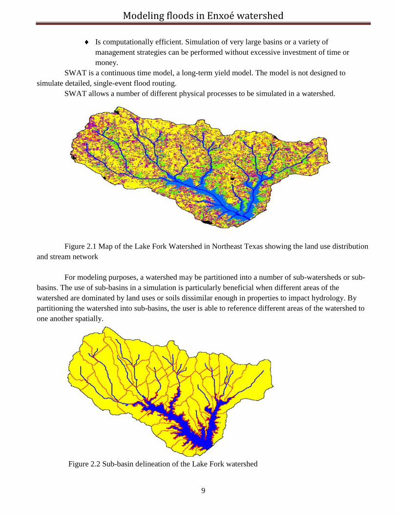
Figure 2.1 Map of the Lake Fork Watershed in Northeast Texas showing the land use distribution

and stream network

For modeling purposes, a watershed may be partitioned into a number of sub-watersheds or sub-

basins. The use of sub-basins in a simulation is particularly beneficial when different areas of the

watershed are dominated by land uses or soils dissimilar enough in properties to impact hydrology. By

partitioning the watershed into sub-basins, the user is able to reference different areas of the watershed to

one another spatially.

Figure 2.2 Sub-basin delineation of the Lake Fork watershed

Modeling floods in Enxoé watershed

10

Input information for each sub-basin is grouped or organized into the following categories:

climate, hydrologic response units or HRUs; ponds/wetlands; groundwater; and the main channel, or

reach, draining the sub-basin. Hydrologic response units are lumped land areas within the sub-basin that

are comprised of unique land cover, soil, and management combinations.

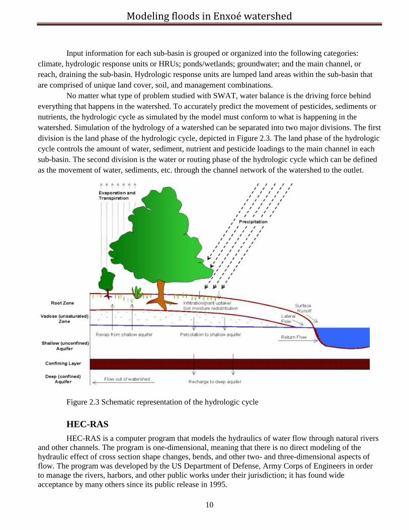
No matter what type of problem studied with SWAT, water balance is the driving force behind

everything that happens in the watershed. To accurately predict the movement of pesticides, sediments or

nutrients, the hydrologic cycle as simulated by the model must conform to what is happening in the

watershed. Simulation of the hydrology of a watershed can be separated into two major divisions. The first

division is the land phase of the hydrologic cycle, depicted in Figure 2.3. The land phase of the hydrologic

cycle controls the amount of water, sediment, nutrient and pesticide loadings to the main channel in each

sub-basin. The second division is the water or routing phase of the hydrologic cycle which can be defined

as the movement of water, sediments, etc. through the channel network of the watershed to the outlet.

Figure 2.3 Schematic representation of the hydrologic cycle

HEC-RAS

HEC-RAS is a computer program that models the hydraulics of water flow through natural rivers

and other channels. The program is one-dimensional, meaning that there is no direct modeling of the

hydraulic effect of cross section shape changes, bends, and other two- and three-dimensional aspects of

flow. The program was developed by the US Department of Defense, Army Corps of Engineers in order

to manage the rivers, harbors, and other public works under their jurisdiction; it has found wide

acceptance by many others since its public release in 1995.

Modeling floods in Enxoé watershed

11

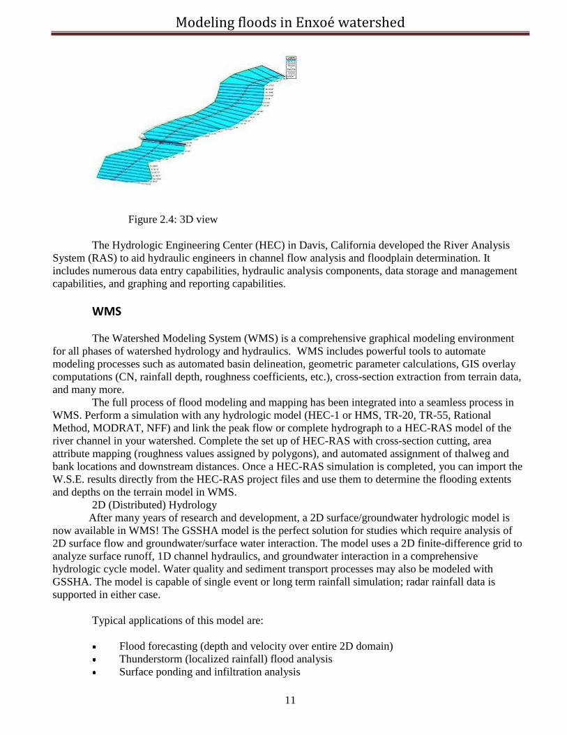
Figure 2.4: 3D view

The Hydrologic Engineering Center (HEC) in Davis, California developed the River Analysis

System (RAS) to aid hydraulic engineers in channel flow analysis and floodplain determination. It

includes numerous data entry capabilities, hydraulic analysis components, data storage and management

capabilities, and graphing and reporting capabilities.

WMS

The Watershed Modeling System (WMS) is a comprehensive graphical modeling environment

for all phases of watershed hydrology and hydraulics. WMS includes powerful tools to automate

modeling processes such as automated basin delineation, geometric parameter calculations, GIS overlay

computations (CN, rainfall depth, roughness coefficients, etc.), cross-section extraction from terrain data,

and many more.

The full process of flood modeling and mapping has been integrated into a seamless process in

WMS. Perform a simulation with any hydrologic model (HEC-1 or HMS, TR-20, TR-55, Rational

Method, MODRAT, NFF) and link the peak flow or complete hydrograph to a HEC-RAS model of the

river channel in your watershed. Complete the set up of HEC-RAS with cross-section cutting, area

attribute mapping (roughness values assigned by polygons), and automated assignment of thalweg and

bank locations and downstream distances. Once a HEC-RAS simulation is completed, you can import the

W.S.E. results directly from the HEC-RAS project files and use them to determine the flooding extents

and depths on the terrain model in WMS.

2D (Distributed) Hydrology

After many years of research and development, a 2D surface/groundwater hydrologic model is

now available in WMS! The GSSHA model is the perfect solution for studies which require analysis of

2D surface flow and groundwater/surface water interaction. The model uses a 2D finite-difference grid to

analyze surface runoff, 1D channel hydraulics, and groundwater interaction in a comprehensive

hydrologic cycle model. Water quality and sediment transport processes may also be modeled with

GSSHA. The model is capable of single event or long term rainfall simulation; radar rainfall data is

supported in either case.

Typical applications of this model are:

Flood forecasting (depth and velocity over entire 2D domain)

Thunderstorm (localized rainfall) flood analysis

Surface ponding and infiltration analysis

Modeling floods in Enxoé watershed

12

Groundwater/surface water interaction modeling

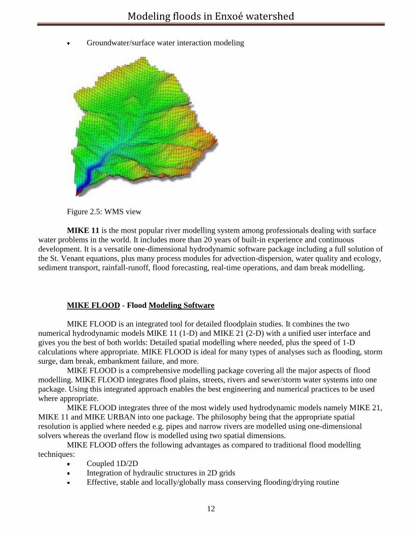
Figure 2.5: WMS view

MIKE 11 is the most popular river modelling system among professionals dealing with surface

water problems in the world. It includes more than 20 years of built-in experience and continuous

development. It is a versatile one-dimensional hydrodynamic software package including a full solution of

the St. Venant equations, plus many process modules for advection-dispersion, water quality and ecology,

sediment transport, rainfall-runoff, flood forecasting, real-time operations, and dam break modelling.

MIKE FLOOD - Flood Modeling Software

MIKE FLOOD is an integrated tool for detailed floodplain studies. It combines the two

numerical hydrodynamic models MIKE 11 (1-D) and MIKE 21 (2-D) with a unified user interface and

gives you the best of both worlds: Detailed spatial modelling where needed, plus the speed of 1-D

calculations where appropriate. MIKE FLOOD is ideal for many types of analyses such as flooding, storm

surge, dam break, embankment failure, and more.

MIKE FLOOD is a comprehensive modelling package covering all the major aspects of flood

modelling. MIKE FLOOD integrates flood plains, streets, rivers and sewer/storm water systems into one

package. Using this integrated approach enables the best engineering and numerical practices to be used

where appropriate.

MIKE FLOOD integrates three of the most widely used hydrodynamic models namely MIKE 21,

MIKE 11 and MIKE URBAN into one package. The philosophy being that the appropriate spatial

resolution is applied where needed e.g. pipes and narrow rivers are modelled using one-dimensional

solvers whereas the overland flow is modelled using two spatial dimensions.

MIKE FLOOD offers the following advantages as compared to traditional flood modelling

techniques:

Coupled 1D/2D

Integration of hydraulic structures in 2D grids

Effective, stable and locally/globally mass conserving flooding/drying routine

Modeling floods in Enxoé watershed

13

Applied for riverine, urban and coastal flood mapping

Accurate and physically based simulation of flow splits

Extensive user support and documentation.

MIKE FLOOD relieves the modeller of the burden of having to choose between the number of

horizontal dimensions and the often-prohibitive resolution requirements of modeling in a detailed 2D

grid. With MIKE FLOOD it is not an either or. Since MIKE FLOOD consists of both 1D and 2D solvers

the modeller can combine these as they see fit.

Typically the 1D model may be used

1. to represent flow in channels that may not be resolved in the 2D grid,

2. to model underlying pipe and sewer networks

3. to simulate hydraulic structures such as culverts, bridges, weirs etc. and

4. to simulate dam or levee failures

5. to route flow in longer river reaches for which a 2D models would be computationally

heavy.

Whereas the 2D model is normally used

1. to represent over bank flows, an application where 1D modeling may be insufficient. A 2D

model has the advantage of being able to accurately represent the floodplain geometry, so that discharge,

storage, and attenuation in the floodplain can be accurately simulated.

2. to relieve the modeller of the burden of having to pre-define the flow paths, the 2D model

will simulate flow splits based on the input topography.

3. to describe the complex network of streets and path ways found in urban areas.

TUFLOW TUFLOW is a powerful computational engine that provides one-dimensional (1D) and two-

dimensional (2D) solutions of the free-surface flow equations to simulate flood and tidal wave

propagation. TUFLOW also leads the way in 2D/1D flood modelling with unparalleled 1D/2D linking,

flexibility, robustness and a range of features no other product provides.

Applicability River flooding

Urban flooding

Pipe network modelling

Storm tide and tsunami inundation

Estuarine and coastal tidal hydraulics

TUFLOW is ideally suited to modelling:

flooding of rivers and creeks with complex flow patterns

overland and piped flows through urban areas

estuarine and coastal tide hydraulics

inundation from storm tides and tsunamis

TUFLOW offers unparalleled 1D/2D and 1D/1D dynamic linking capabilities with other

products.

The TUFLOW engine interfaces with GIS software such as MapInfo, ArcGIS or SAGA and/or

via the Aquaveo SMS GUI. 12D Solutions are developing a customized TUFLOW interface and

WaterRIDE displays, animates and post-processes TUFLOW output.

Modeling floods in Enxoé watershed

14

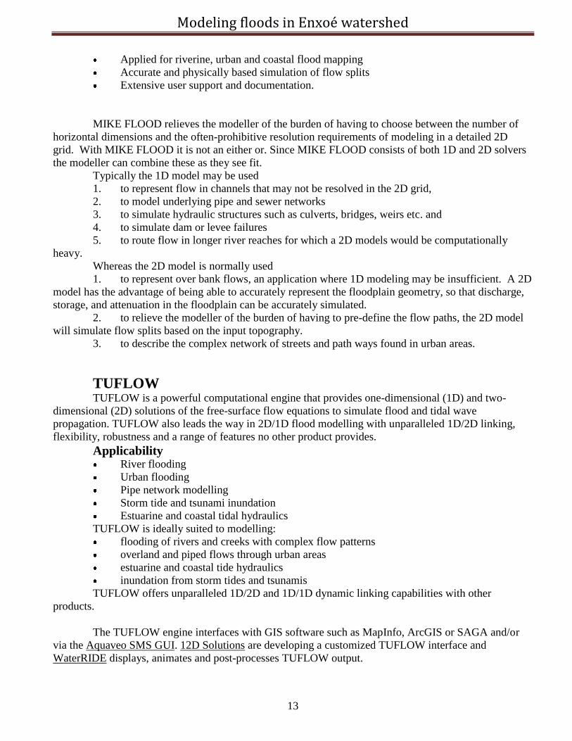
TUFLOW is the dominant 2D flood modeling software in the UK, and is the most widely used

1D/2D flood modelling software in Australia. In 2010, TUFLOW and XP-2D were given FEMA approval

in the USA.

Figure 2.6: Estuarine application

SOBEK, an one and two dimensional integrated modelling framework for integral water

solutions

SOBEK is a powerful modelling framework for flood forecasting, optimization of drainage

systems, control of irrigation systems, sewer overflow design, river morphology, salt intrusion and surface

water quality. The components within the SOBEK modelling framework simulate the complex flows and

the water related processes in almost any system. The components represent phenomena and physical

processes in an accurate way in one dimensional (1D) network systems and on two dimensional (2D)

horizontal grids.

SOBEK offers one software environment for the simulation of all management problems in the

areas of river and estuarine systems, drainage and irrigation systems and wastewater and storm water

systems. This allows for combinations of flow in closed conduits, open channels, rivers overland flows, as

well as a variety of hydraulic, hydrological and environmental processes.

ISIS FAST

ISIS FAST is an innovative flood inundation modelling tool designed to allow quick assessment

of flooding using simplified hydraulics. It provides results in seconds or minutes as opposed to hours or

days, which is up to 1,000 times faster than traditional two-dimensional models.

Modeling floods in Enxoé watershed

15

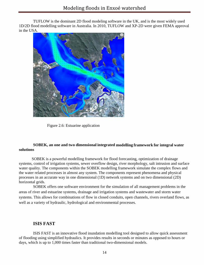
The software works by first identifying depressions on the floodplain then routing water through

these depressions. Water depths in the depressions are determined by the volume of water flowing into

each one, the level at which water can spill into neighboring depressions and the water level in the

neighboring depressions. ISIS FAST is able to do this by adopting new and innovative ways of resolving

the detailed hydraulics.

ISIS FAST allows modellers to rapidly estimate flood extents and depths from multiple sources

of water, including tide, surge and fluvial overtopping or breaching of defences, surface water and sewer

flooding. The speed with which it can calculate water depths gives modellers the flexibility to explore

uncertainty. Event magnitude and the interactions and dependency between flood sources were previously

unpractical or economical. The application of ISIS FAST includes near real-time flood inundation prediction on the Tidal Thames in

London through to prediction of areas susceptible to pluvial flooding for the whole of Scotland.

Key features of ISIS FAST:

rapidly estimates flood extents and depths from many sources of flooding, including

coastal, fluvial, surface water and sewer flooding

pluvial flood mapping and risk assessments at local, regional and national scales

real-time flood mapping when linked to forecast rainfall

used in conjunction with more detailed modelling software, such as ISIS Professional and

ISIS 2D

can remove the cost of some detailed modelling by identifying the flood risk hot spots

where detailed analysis is needed

can be used in probabilistic analysis frameworks

can test solutions that protect people, property, critical infrastructure and the urban

environment.

Modeling floods in Enxoé watershed

16

3rd

Chapter . MOHID Land. Model description

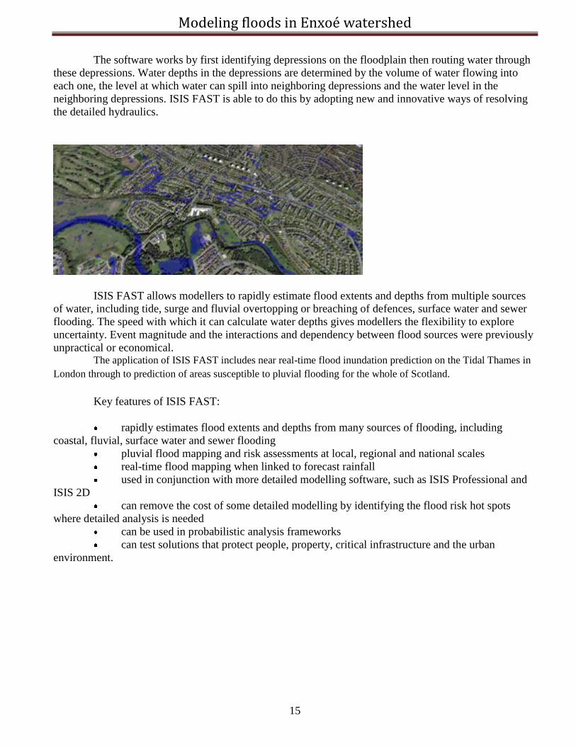
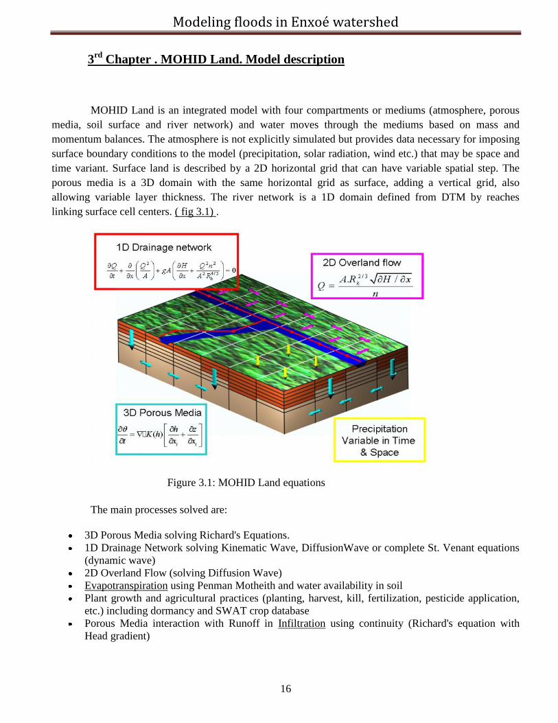
MOHID Land is an integrated model with four compartments or mediums (atmosphere, porous

media, soil surface and river network) and water moves through the mediums based on mass and

momentum balances. The atmosphere is not explicitly simulated but provides data necessary for imposing

surface boundary conditions to the model (precipitation, solar radiation, wind etc.) that may be space and

time variant. Surface land is described by a 2D horizontal grid that can have variable spatial step. The

porous media is a 3D domain with the same horizontal grid as surface, adding a vertical grid, also

allowing variable layer thickness. The river network is a 1D domain defined from DTM by reaches

linking surface cell centers. ( fig 3.1) .

Figure 3.1: MOHID Land equations

The main processes solved are:

3D Porous Media solving Richard's Equations.

1D Drainage Network solving Kinematic Wave, DiffusionWave or complete St. Venant equations

(dynamic wave)

2D Overland Flow (solving Diffusion Wave)

Evapotranspiration using Penman Motheith and water availability in soil

Plant growth and agricultural practices (planting, harvest, kill, fertilization, pesticide application,

etc.) including dormancy and SWAT crop database

Porous Media interaction with Runoff in Infiltration using continuity (Richard's equation with

Head gradient)

Modeling floods in Enxoé watershed

17

Porous Media and Runoff interaction with Drainage Network using continuity (surface gradient

between Runoff and Drainage Network. Richard's equation with level gradient between Porous

Media and Drainage Network)

Property transport in all mediums and transformation in soil and river (water quality models can be

coupled)

Biological and chemical reactions in soil as mineralization, nitrification, denitrification,

immobilization, chemical equilibrium, property decay, and processes in river as primary

production, nutrient assimilation, property decay, etc.

Linkage to MOHID Water by Module Discharges

Floods.

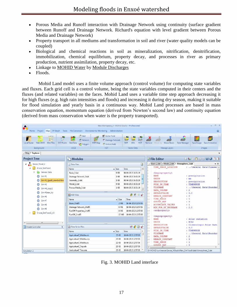
Mohid Land model uses a finite volume approach (control volume) for computing state variables

and fluxes. Each grid cell is a control volume, being the state variables computed in their centers and the

fluxes (and related variables) on the faces. Mohid Land uses a variable time step approach decreasing it

for high fluxes (e.g. high rain intensities and floods) and increasing it during dry season, making it suitable

for flood simulation and yearly basis in a continuous way. Mohid Land processes are based in mass

conservation equation, momentum equation (derived from Newton’s second law) and continuity equation

(derived from mass conservation when water is the property transported).

Fig. 3. MOHID Land interface

Modeling floods in Enxoé watershed

18

MOHID Land Modules

Some modules developed are related with specific processes which occur inside a watershed and

on a specific medium, creating thus a modular structure. For user first approach and advanced use,

processes solved, equations, input data files examples are presented below for each MOHID Land module:

Module PorousMedia which calculates infiltration, unsaturated and saturated water

movement

Module PorousMediaProperties which calculates property transport and

transformation in soil.

Module SedimentQuality which calculates property transformation in soil driven by

microorgansims (mineralization, nitrification, denitrification, etc.).

Module PREEQC which calculates property transformation in soil through chemical

equilibrium.

Module Runoff which calculates overland runoff;

Module RunoffProperties which calculates property transport in runoff.

Module DrainageNetwork which handles water and property routing and property

transformation inside rivers.

Module Vegetation which handles vegetation growth and agricultural practices.

Module Basin which handles information between modules and computes interface

forcing fluxes between atmosphere and soil (e.g. throughfall, potential

evapotranspiration, etc.).

MOHID Land also uses all the modules for data pre-processing, computation and post-processing

that are common to MOHID Water (e.g. data file read, geometry handling, results writing in HDF and

time serie, etc.) See below how you can see module source code.

Module Runoff

Module Runoff allows the calculation of the overland surface runoff over a grid as function of the water column slopes between adjacent cells (dynamic wave). The water column, namely the water located above the terrain, is given by the Module Basin after considering the precipitation input and the losses due to the evaporation and the infiltration. Overland flow is evaluated by the Manning’s equation.

Main Processes

Manning Equation

The overland surface runoff flow (m3/s) is calculated at the cell faces and it is obtained by

applying the Manning's equation <ref>Gauckler, P. (1867), Etudes Théoriques et Pratiques sur

l'Ecoulement et le Mouvement des Eaux, Comptes Rendues de l'Académie des Sciences, Paris, France,

Tome 64, pp. 818–822</ref> :

2 1

3 21

hQ A R sn

where:

Q is the overland flow (m3/s)

Modeling floods in Enxoé watershed

19

A is the area of the cross-section (m2)

n is the Manning coefficient (s/m1/3

)

Rh is the hydraulic radius (m)

S is the slope of the water surface (m/m)

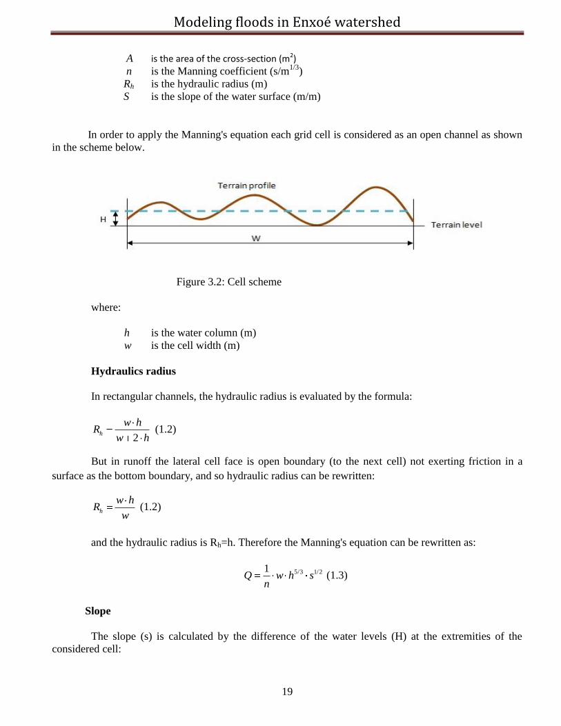
In order to apply the Manning's equation each grid cell is considered as an open channel as shown

in the scheme below.

Figure 3.2: Cell scheme

where:

h is the water column (m)

w is the cell width (m)

Hydraulics radius

In rectangular channels, the hydraulic radius is evaluated by the formula:

2h

w hR

w h (1.2)

But in runoff the lateral cell face is open boundary (to the next cell) not exerting friction in a

surface as the bottom boundary, and so hydraulic radius can be rewritten:

h

w hR

w (1.2)

and the hydraulic radius is Rh=h. Therefore the Manning's equation can be rewritten as:

5/3 1/21Q w h s

n (1.3)

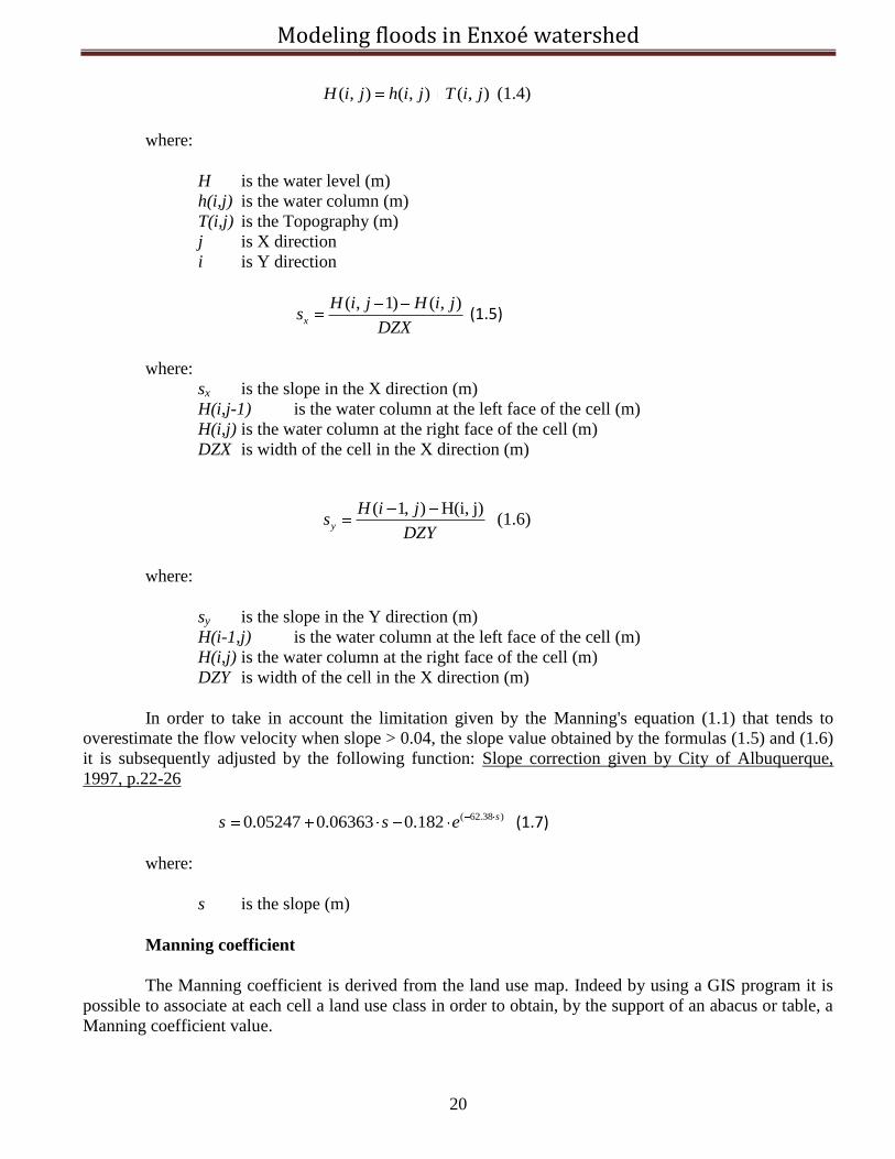
Slope

The slope (s) is calculated by the difference of the water levels (H) at the extremities of the

considered cell:

Modeling floods in Enxoé watershed

20

( , ) ( , ) ( , )H i j h i j T i j (1.4)

where:

H is the water level (m)

h(i,j) is the water column (m)

T(i,j) is the Topography (m)

j is X direction

i is Y direction

( , 1) ( , )x

H i j H i js

DZX (1.5)

where:

sx is the slope in the X direction (m)

H(i,j-1) is the water column at the left face of the cell (m)

H(i,j) is the water column at the right face of the cell (m)

DZX is width of the cell in the X direction (m)

( 1, ) H(i, j)

y

H i js

DZY (1.6)

where:

sy is the slope in the Y direction (m)

H(i-1,j) is the water column at the left face of the cell (m)

H(i,j) is the water column at the right face of the cell (m)

DZY is width of the cell in the X direction (m)

In order to take in account the limitation given by the Manning's equation (1.1) that tends to

overestimate the flow velocity when slope > 0.04, the slope value obtained by the formulas (1.5) and (1.6)

it is subsequently adjusted by the following function: Slope correction given by City of Albuquerque,

1997, p.22-26

( 62.38 )0.05247 0.06363 0.182 ss s e (1.7)

where:

s is the slope (m)

Manning coefficient

The Manning coefficient is derived from the land use map. Indeed by using a GIS program it is

possible to associate at each cell a land use class in order to obtain, by the support of an abacus or table, a

Manning coefficient value.

Modeling floods in Enxoé watershed

21

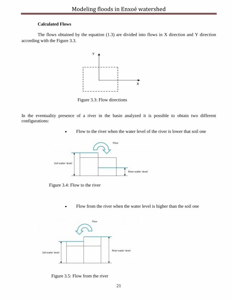
Calculated Flows

The flows obtained by the equation (1.3) are divided into flows in X direction and Y direction

according with the Figure 3.3.

Figure 3.3: Flow directions

In the eventuality presence of a river in the basin analyzed it is possible to obtain two different

configurations:

Flow to the river when the water level of the river is lower that soil one

Figure 3.4: Flow to the river

Flow from the river when the water level is higher than the soil one

Figure 3.5: Flow from the river

Modeling floods in Enxoé watershed

22

The flow between river and runoff is computed using the same formulation as in runoff cells using the

surface gradient between runoff and river.

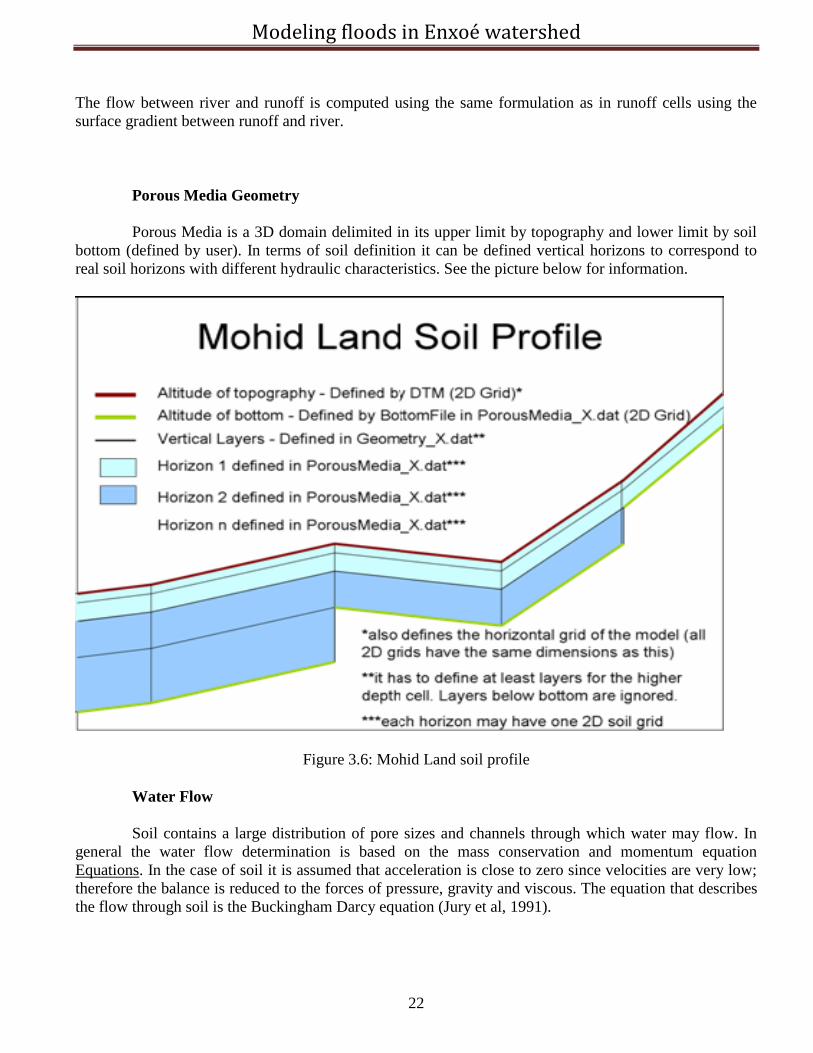
Porous Media Geometry

Porous Media is a 3D domain delimited in its upper limit by topography and lower limit by soil

bottom (defined by user). In terms of soil definition it can be defined vertical horizons to correspond to

real soil horizons with different hydraulic characteristics. See the picture below for information.

Figure 3.6: Mohid Land soil profile

Water Flow

Soil contains a large distribution of pore sizes and channels through which water may flow. In

general the water flow determination is based on the mass conservation and momentum equation

Equations. In the case of soil it is assumed that acceleration is close to zero since velocities are very low;

therefore the balance is reduced to the forces of pressure, gravity and viscous. The equation that describes

the flow through soil is the Buckingham Darcy equation (Jury et al, 1991).

Modeling floods in Enxoé watershed

23

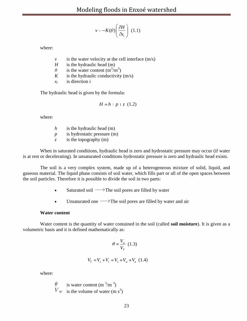
( )i

Hv K

x (1.1)

where:

v is the water velocity at the cell interface (m/s)

H is the hydraulic head (m)

θ is the water content (m3/m

3)

K is the hydraulic conductivity (m/s)

xi is direction i

The hydraulic head is given by the formula:

H h p z (1.2)

where:

h is the hydraulic head (m)

p is hydrostatic pressure (m)

z is the topography (m)

When in saturated conditions, hydraulic head is zero and hydrostatic pressure may occur (if water

is at rest or decelerating). In unsaturated conditions hydrostatic pressure is zero and hydraulic head exists.

The soil is a very complex system, made up of a heterogeneous mixture of solid, liquid, and

gaseous material. The liquid phase consists of soil water, which fills part or all of the open spaces between

the soil particles. Therefore it is possible to divide the soil in two parts:

Saturated soil The soil pores are filled by water

Unsaturated one The soil pores are filled by water and air

Water content

Water content is the quantity of water contained in the soil (called soil moisture). It is given as a

volumetric basis and it is defined mathematically as:

w

T

V

V (1.3)

T s v s w aV V V V V V (1.4)

where:

is water content (m 3/m

3)

is the volume of water (m s3)

Modeling floods in Enxoé watershed

24

is the total volume (m 3)

is the soil volume (m 3)

is the air space (m 3)

Module Basin

Module Basin works as an interface among the different modules of Mohid-Land. Indeed it

manages fluxes between modules as precipitation, evapotranspiration, infiltration etc. and updates water

column and concentration after each module call. This module is able to compute a water and mass

balance for each property transported in all mediums.

Main Processes

The processes made in the Module Basin can be summarized as following:

Reading entering data and grid construction

Atmospheric processes (precipitation, leaf interception, leaf drainage, evaporation)

in order to obtain the potential water column

Call of Module PorousMedia giving potential water column and obtain the

infiltration rate

Update of the water column and send it to ModuleRunoff (the holder of water

column)

Call of Module PorousMediaProperties and update of water column concentrations

send it to the ModuleRunoffProperties

Call of Module Runoff giving the remaining water columns to be transported

Call of Module RunoffProperties

(When Module Runoff and RunoffProperties run as they are the holders of water column and

water column concentration, no update is needed).

Call of Module DrainageNetwork to route the water in the river and the new

transfered from groundwater and from runoff.

Output of the different components of the water and property flux

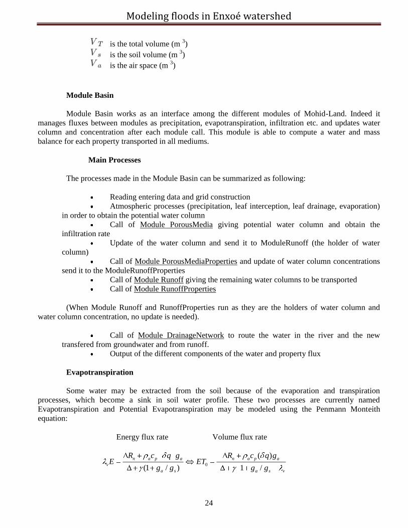
Evapotranspiration

Some water may be extracted from the soil because of the evaporation and transpiration

processes, which become a sink in soil water profile. These two processes are currently named

Evapotranspiration and Potential Evapotranspiration may be modeled using the Penmann Monteith

equation:

Energy flux rate Volume flux rate

0

( )

(1 / ) 1 /

n a p a n a p a

v

a s a s v

R c q g R c q gE ET

g g g g

Modeling floods in Enxoé watershed

25

λv = Latent heat of vaporization. Energy required per unit mass of water vaporized. (J/g)

Lv = Volumetric latent heat of vaporization. Energy required per water volume vaporized.

(Lv = 2453 MJ m-3

)

E = Mass water evapotranspiration rate (g s-1

m-2

)

ETo = Water volume evapotranspired (m3 s

-1 m

-2)

Δ = Rate of change of saturation specific humidity with air temperature. (Pa K-1

)

Rn = Net irradiance (W m-2

), the external source of energy flux

cp = Specific heat capacity of air (J kg-1

K-1

)

ρa = dry air density (kg m-3

)

δe = vapor pressure deficit, or specific humidity (Pa)

ga = Hydraulic conductivity of air, atmospheric conductance (m s-1

)

gs = Conductivity of stoma, surface conductance (m s-1

)

γ = Psychrometric constant (γ ≈ 66 Pa K-1

)

Mohid Land has a sub-daily time step. According with FAO-56 Hourly Time Step ET is

calculated with the equation below. This is the equation used in Mohid-Land.

0

2 )

0

2

37408 ( ) (

273

(1 0.34 )

n h a

h

R G u e T eT

ETu

ETo = reference evapotranspiration [mm hour-1]

Rn = net radiation at the grass surface [MJ m-2 hour-1]

G = soil heat flux density [MJ m-2 hour-1]

Th = mean hourly air temperature at 2m hight [°C]

Δ = saturation slope vapour pressure curve at Th [kPa °C-1]

γ = psychrometric constant [kPa °C-1]

e°(Th) = saturation vapour pressure at air temperature Th [kPa]

ea = average hourly actual vapour pressure [kPa]

u2 = average hourly wind speed at 2m hight [m s-1].

Calculate Psychrometric constant:

p air

p ratio

c P

MW

psychrometric constant [kPa °C-1

],

P = atmospheric pressure [kPa],

v = latent heat of water vaporization, 2.45 [MJ kg-1

],

pc = specific heat of air at constant pressure, 1.013 10-3 [MJ kg-1

°C-1

],

MWratio = ratio molecular weight of water vapor/dry air = 0.622.

Equation of becomes:

30.665 10 P

Modeling floods in Enxoé watershed

26

Calculation of the atmospheric pressure based on the heigth simplification of the ideal gas law

5.26293. 0.0065

101.3293.

ElevationP

G beneath a dense cover of grass does not correlate well with air temperature. Hourly G can be

approximated during daylight periods as: G=0.1Rn and during nighttime periods as: G=0.5Rn

The net radiation (Rn) is the difference between the incoming net shortwave radiation (Rns) and

the outgoing net long wave radiation (Rnl):

1 0.23 5.669 0.8 273.15 4hRn Rns Rnl SolarRadiation e T LwradCorrection

0.34 0.14 0.5 1.35 0.35LwradCorrection VP ATMTransmitivity

The Penman Montheith Potential Evapotranspiration computation will be active if in basin file

EVAPOTRANSPIRATION: 1

and the property evapotranspiration is not read from file.

If the user is running with vegetation than Crop Evapotranspiration is obtained from Potential

Evapotranspiration using crop coefficient from Module Vegetation (dependent on crop).

Also if the user is running with vegetation a differentiation in Crop Evapotranspiration between Potential Transpiration and Potential Evaporation may be done using LAI:

EVAPOTRANSPIRATION_METHOD: 2

3.2 Description of study area

Portugal, is a country located in Southwestern Europe, on the Iberian Peninsula. It is the

westernmost country of mainland Europe, and is bordered by the Atlantic Ocean to the west and south and

by Spain to the north and east. Apart from continental Portugal, the Portuguese Republic holds

sovereignty over the Atlantic archipelagos of Azores and Madeira, which are autonomous regions of

Portugal. The country is named after its second largest city, Porto, whose Latin name was Portus Cale.

Modeling floods in Enxoé watershed

27

3.2.1 Enxoé catchment description:

General characteristics

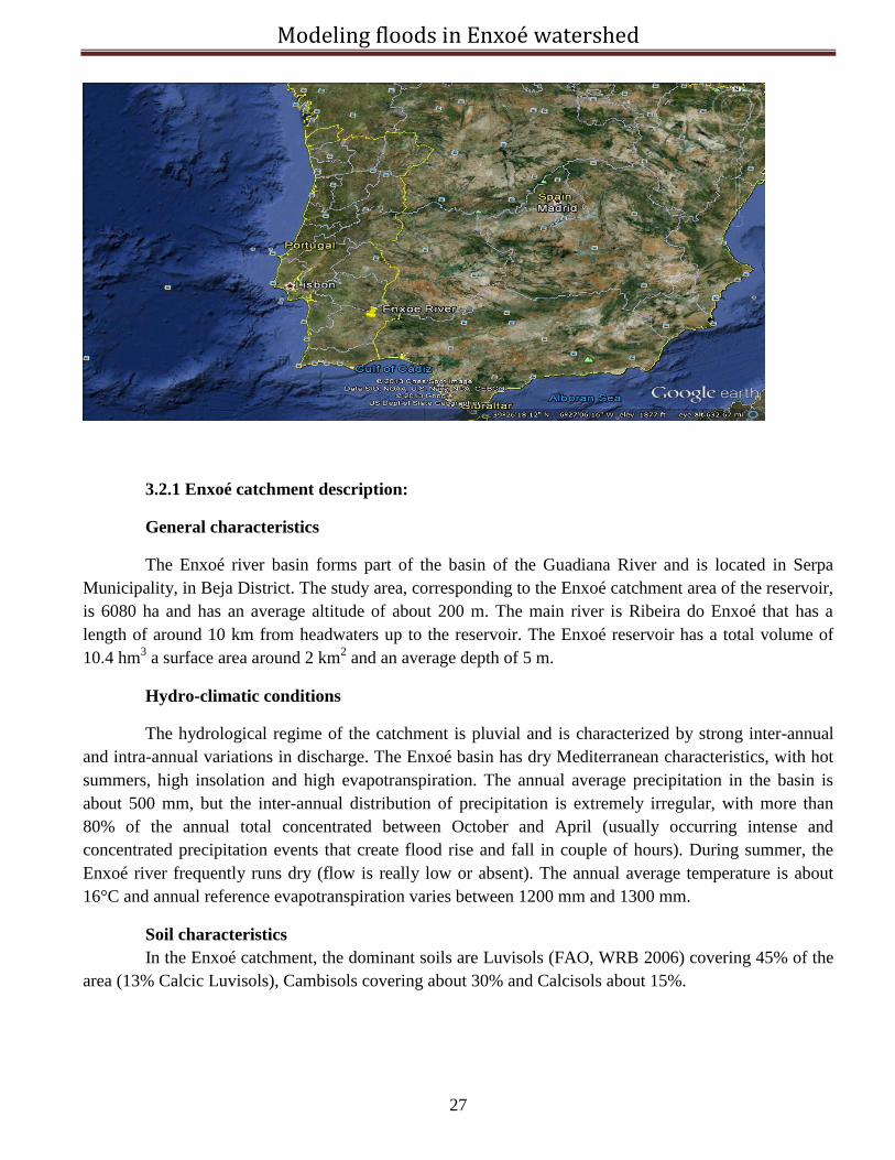
The Enxoé river basin forms part of the basin of the Guadiana River and is located in Serpa

Municipality, in Beja District. The study area, corresponding to the Enxoé catchment area of the reservoir,

is 6080 ha and has an average altitude of about 200 m. The main river is Ribeira do Enxoé that has a

length of around 10 km from headwaters up to the reservoir. The Enxoé reservoir has a total volume of

10.4 hm3 a surface area around 2 km

2 and an average depth of 5 m.

Hydro-climatic conditions

The hydrological regime of the catchment is pluvial and is characterized by strong inter-annual

and intra-annual variations in discharge. The Enxoé basin has dry Mediterranean characteristics, with hot

summers, high insolation and high evapotranspiration. The annual average precipitation in the basin is

about 500 mm, but the inter-annual distribution of precipitation is extremely irregular, with more than

80% of the annual total concentrated between October and April (usually occurring intense and

concentrated precipitation events that create flood rise and fall in couple of hours). During summer, the

Enxoé river frequently runs dry (flow is really low or absent). The annual average temperature is about

16°C and annual reference evapotranspiration varies between 1200 mm and 1300 mm.

Soil characteristics

In the Enxoé catchment, the dominant soils are Luvisols (FAO, WRB 2006) covering 45% of the

area (13% Calcic Luvisols), Cambisols covering about 30% and Calcisols about 15%.

Modeling floods in Enxoé watershed

28

Land use

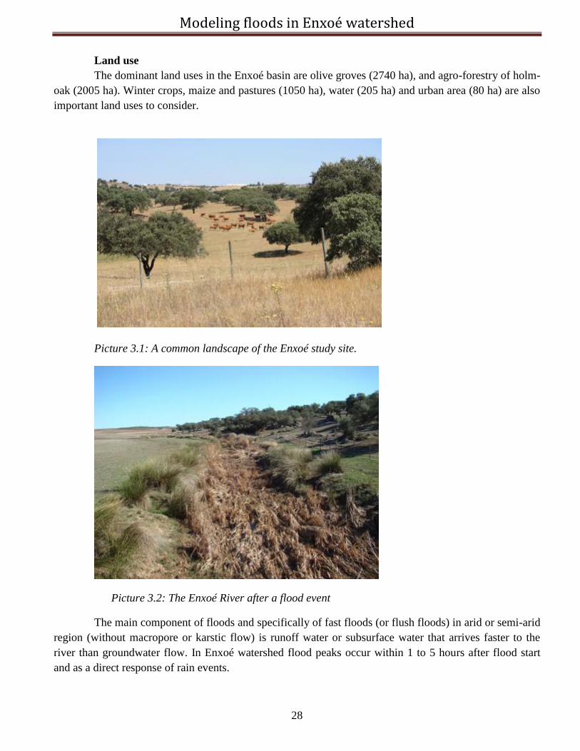
The dominant land uses in the Enxoé basin are olive groves (2740 ha), and agro-forestry of holm-

oak (2005 ha). Winter crops, maize and pastures (1050 ha), water (205 ha) and urban area (80 ha) are also

important land uses to consider.

Picture 3.1: A common landscape of the Enxoé study site.

Picture 3.2: The Enxoé River after a flood event

The main component of floods and specifically of fast floods (or flush floods) in arid or semi-arid

region (without macropore or karstic flow) is runoff water or subsurface water that arrives faster to the

river than groundwater flow. In Enxoé watershed flood peaks occur within 1 to 5 hours after flood start

and as a direct response of rain events.

Modeling floods in Enxoé watershed

29

The process of runoff generation in flush floods may have origin in water that is unable to

infiltrate (because of soil impermeabilization or storm water drainage in urban areas) or if infiltration in

soil occurs, the predominance of infiltration excess, subsurface stormflow or saturation excess will depend

on rain intensity, soil properties (e.g. conductivity, water content etc) and slope.

One aspect that may influence flood formation is soil sealing as reduces infiltration and promotes

runoff formation. Soil surface sealing may result from:

- Compaction (e.g. livestock, urban impermeabilization);

- Fire

- Biological activity

- Rain

Rain may also have a compact effect, destroy soil aggregates and the released material may fill

soil pores – locally generated or transported by runoff. In Enxoé, silty soils occur and approximately 60%

of the total area (occupied by olive trees and annual crops) has tillage and/or wheeling and in montado

area (30% of the total area) extensive cattle production exists. The observation in Enxoé of river flood

events even after dry season as a direct response to first rain events, suggest that soil sealing and/or

compaction/impermeabilization may be an important process on first flood formation.

Monitoring data is usually scarce, especially in cases where floods rise within minutes to hours

and collection frequency need to be high (need for automatic schemes that are costly). As so, in order to

fill data gaps and to be able to predict their occurrence, models have been developed especially suited for

floods.

The first feature needed to simulate a flood is that the model has to have a time step that can

represent the flood rise and fall; in flush floods that may represent hourly or sub-hourly time steps

(Boughton and Droop, 2003). The second feature, since in flush floods most of the water in the river

arrives from surface water or storm drainage systems (in urban areas) than the model should be able to

simulate impermeabilization, runoff generation and routing and storm drainage systems (Hsu et al. 2000).

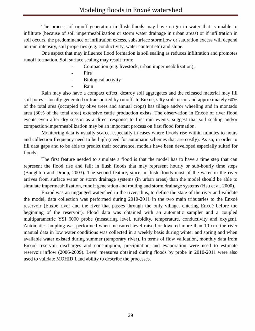
Enxoé was an ungauged watershed in the river, thus, to define the state of the river and validate

the model, data collection was performed during 2010-2011 in the two main tributaries to the Enxoé

reservoir (Enxoé river and the river that passes through the only village, entering Enxoé before the

beginning of the reservoir). Flood data was obtained with an automatic sampler and a coupled

multiparametric YSI 6000 probe (measuring level, turbidity, temperature, conductivity and oxygen).

Automatic sampling was performed when measured level raised or lowered more than 10 cm. the river

manual data in low water conditions was collected in a weekly basis during winter and spring and when

available water existed during summer (temporary river). In terms of flow validation, monthly data from

Enxoé reservoir discharges and consumption, precipitation and evaporation were used to estimate

reservoir inflow (2006-2009). Level measures obtained during floods by probe in 2010-2011 were also

used to validate MOHID Land ability to describe the processes.

Modeling floods in Enxoé watershed

30

Fig. 3.7 Enxoé watershed

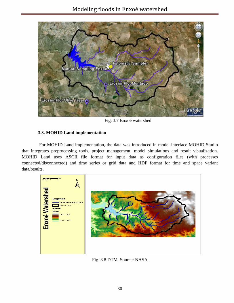
3.3. MOHID Land implementation

For MOHID Land implementation, the data was introduced in model interface MOHID Studio

that integrates preprocessing tools, project management, model simulations and result visualization.

MOHID Land uses ASCII file format for input data as configuration files (with processes

connected/disconnected) and time series or grid data and HDF format for time and space variant

data/results.

Fig. 3.8 DTM. Source: NASA

Modeling floods in Enxoé watershed

31

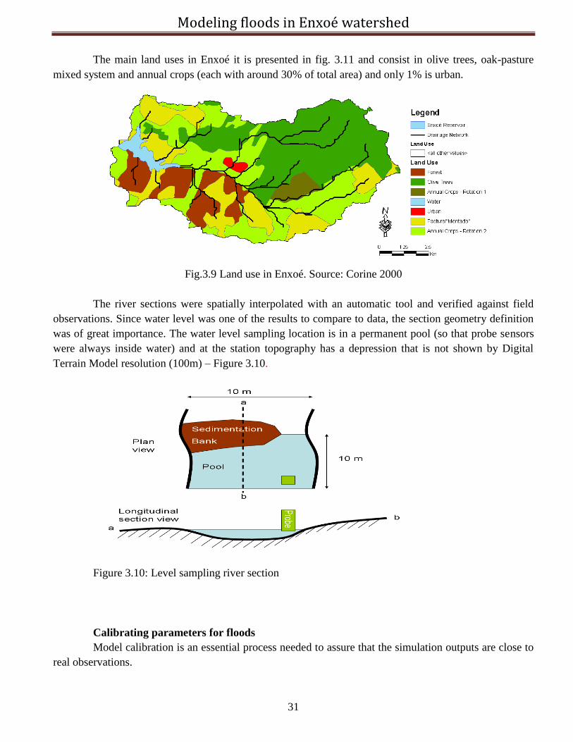
The main land uses in Enxoé it is presented in fig. 3.11 and consist in olive trees, oak-pasture

mixed system and annual crops (each with around 30% of total area) and only 1% is urban.

Fig.3.9 Land use in Enxoé. Source: Corine 2000

The river sections were spatially interpolated with an automatic tool and verified against field

observations. Since water level was one of the results to compare to data, the section geometry definition

was of great importance. The water level sampling location is in a permanent pool (so that probe sensors

were always inside water) and at the station topography has a depression that is not shown by Digital

Terrain Model resolution (100m) – Figure 3.10.

Figure 3.10: Level sampling river section

Calibrating parameters for floods

Model calibration is an essential process needed to assure that the simulation outputs are close to

real observations.

Modeling floods in Enxoé watershed

32

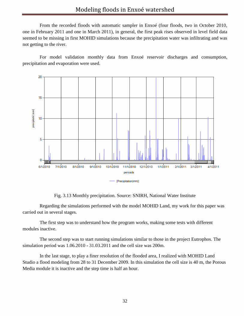
From the recorded floods with automatic sampler in Enxoé (four floods, two in October 2010,

one in February 2011 and one in March 2011), in general, the first peak rises observed in level field data

seemed to be missing in first MOHID simulations because the precipitation water was infiltrating and was

not getting to the river.

For model validation monthly data from Enxoé reservoir discharges and consumption,

precipitation and evaporation were used.

Fig. 3.13 Monthly precipitation. Source: SNIRH, National Water Institute

Regarding the simulations performed with the model MOHID Land, my work for this paper was

carried out in several stages.

The first step was to understand how the program works, making some tests with different

modules inactive.

The second step was to start running simulations similar to those in the project Eutrophos. The

simulation period was 1.06.2010 - 31.03.2011 and the cell size was 200m.

In the last stage, to play a finer resolution of the flooded area, I realized with MOHID Land

Studio a flood modeling from 28 to 31 December 2009. In this simulation the cell size is 40 m, the Porous

Media module it is inactive and the step time is half an hour.

Modeling floods in Enxoé watershed

33

4th

Chapter. Results and Conclusions

4.1 Simulation of the period 1.06.2010 – 31.03.2011

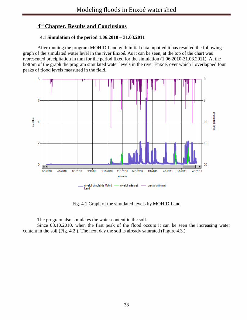
After running the program MOHID Land with initial data inputted it has resulted the following

graph of the simulated water level in the river Enxoé. As it can be seen, at the top of the chart was

represented precipitation in mm for the period fixed for the simulation (1.06.2010-31.03.2011). At the

bottom of the graph the program simulated water levels in the river Enxoé, over which I overlapped four

peaks of flood levels measured in the field.

Fig. 4.1 Graph of the simulated levels by MOHID Land

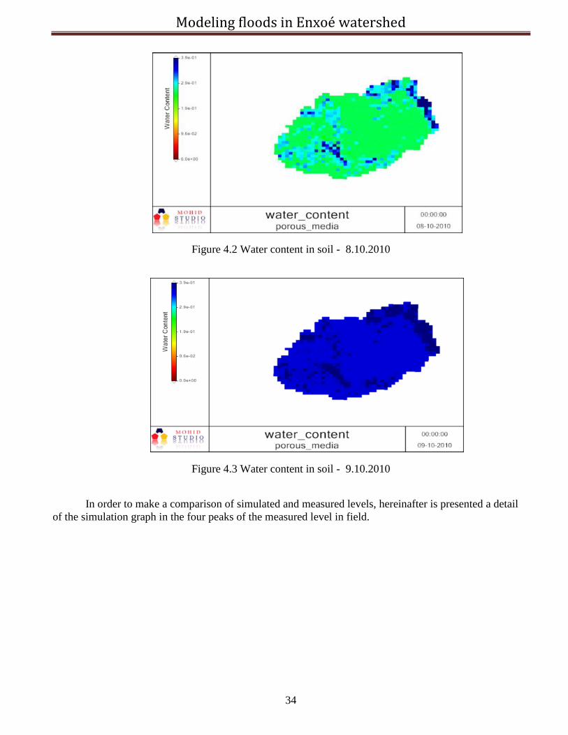
The program also simulates the water content in the soil.

Since 08.10.2010, when the first peak of the flood occurs it can be seen the increasing water

content in the soil (Fig. 4.2.). The next day the soil is already saturated (Figure 4.3.).

Modeling floods in Enxoé watershed

34

Figure 4.2 Water content in soil - 8.10.2010

Figure 4.3 Water content in soil - 9.10.2010

In order to make a comparison of simulated and measured levels, hereinafter is presented a detail

of the simulation graph in the four peaks of the measured level in field.

Modeling floods in Enxoé watershed

35

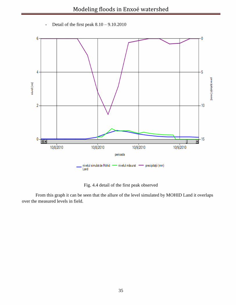
- Detail of the first peak 8.10 – 9.10.2010

Fig. 4.4 detail of the first peak observed

From this graph it can be seen that the allure of the level simulated by MOHID Land it overlaps

over the measured levels in field.

Modeling floods in Enxoé watershed

36

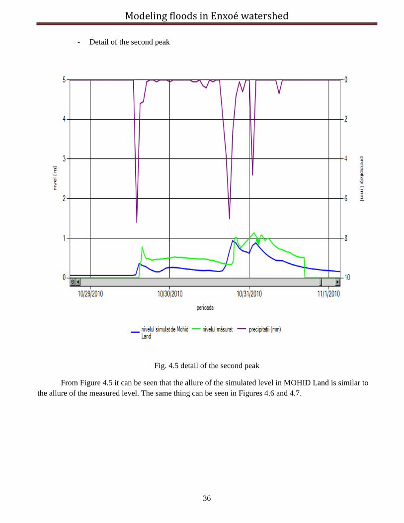
- Detail of the second peak

Fig. 4.5 detail of the second peak

From Figure 4.5 it can be seen that the allure of the simulated level in MOHID Land is similar to

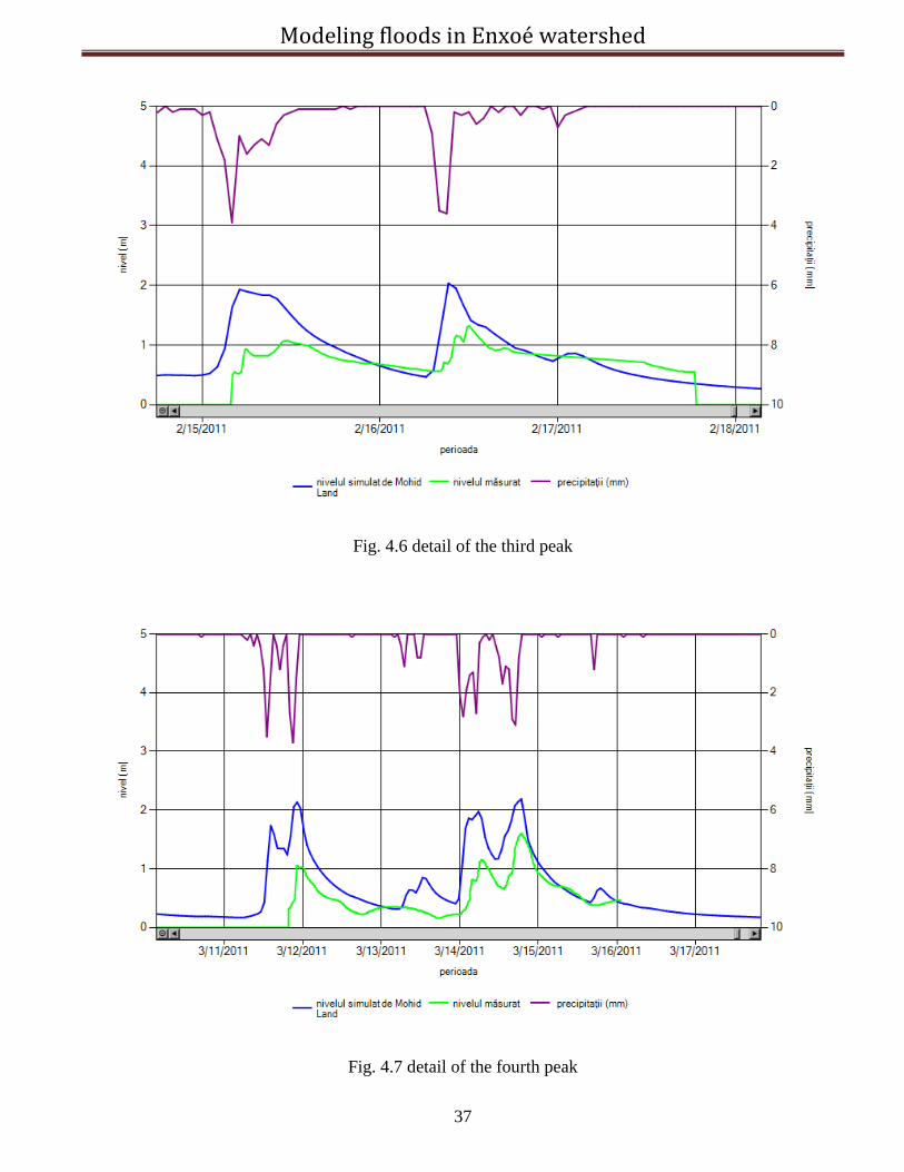
the allure of the measured level. The same thing can be seen in Figures 4.6 and 4.7.

Modeling floods in Enxoé watershed

37

Fig. 4.6 detail of the third peak

Fig. 4.7 detail of the fourth peak

Modeling floods in Enxoé watershed

38

As the results provided by MOHID Land are close to the measurements, further we made a

simulation of the flood from December 2009. For this flood there were no data measured in field.

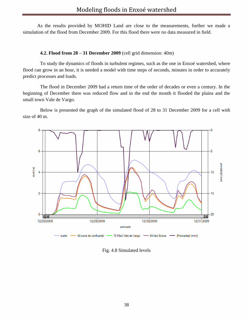
4.2. Flood from 28 – 31 December 2009 (cell grid dimension: 40m)

To study the dynamics of floods in turbulent regimes, such as the one in Enxoé watershed, where

flood can grow in an hour, it is needed a model with time steps of seconds, minutes in order to accurately

predict processes and loads.

The flood in December 2009 had a return time of the order of decades or even a century. In the

beginning of December there was reduced flow and in the end the month it flooded the plains and the

small town Vale de Vargo.

Below is presented the graph of the simulated flood of 28 to 31 December 2009 for a cell with

size of 40 m.

Fig. 4.8 Simulated levels

Modeling floods in Enxoé watershed

39

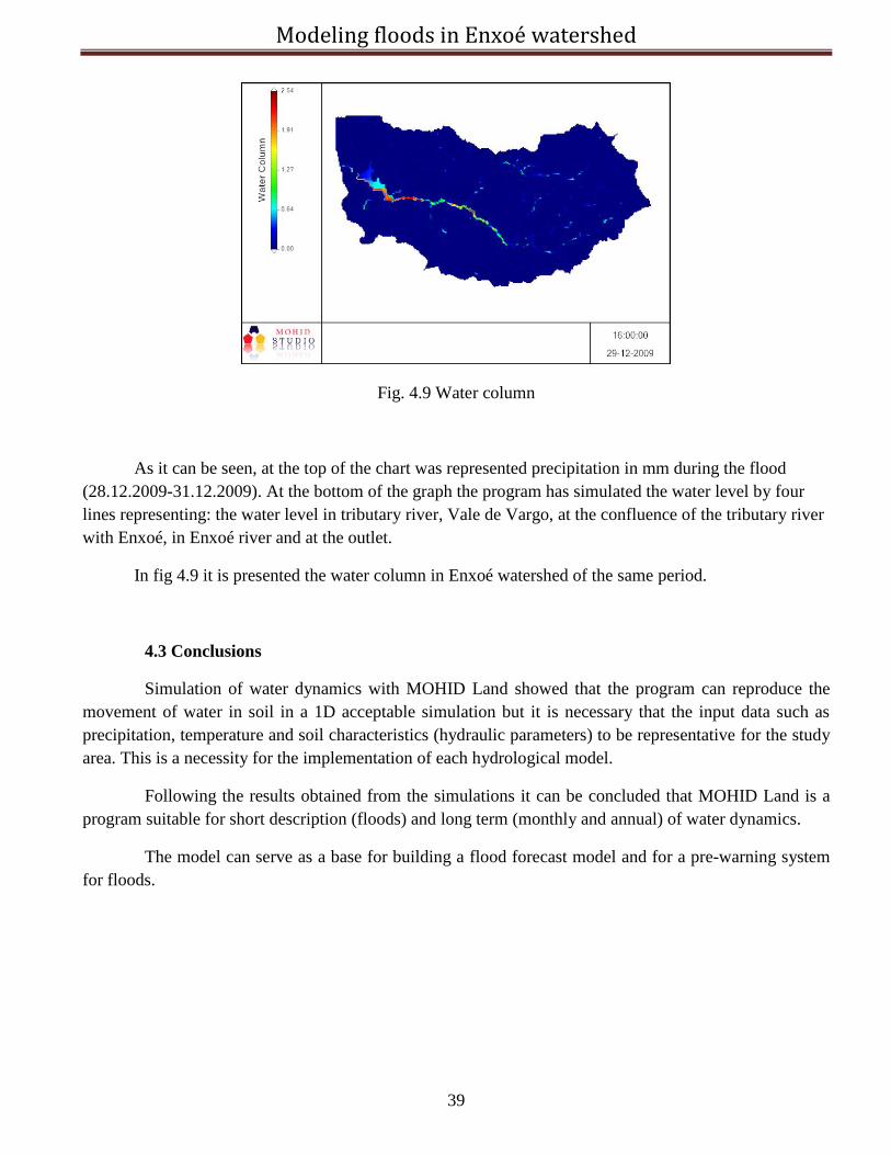
Fig. 4.9 Water column

As it can be seen, at the top of the chart was represented precipitation in mm during the flood

(28.12.2009-31.12.2009). At the bottom of the graph the program has simulated the water level by four

lines representing: the water level in tributary river, Vale de Vargo, at the confluence of the tributary river

with Enxoé, in Enxoé river and at the outlet.

In fig 4.9 it is presented the water column in Enxoé watershed of the same period.

4.3 Conclusions

Simulation of water dynamics with MOHID Land showed that the program can reproduce the

movement of water in soil in a 1D acceptable simulation but it is necessary that the input data such as

precipitation, temperature and soil characteristics (hydraulic parameters) to be representative for the study

area. This is a necessity for the implementation of each hydrological model.

Following the results obtained from the simulations it can be concluded that MOHID Land is a

program suitable for short description (floods) and long term (monthly and annual) of water dynamics.

The model can serve as a base for building a flood forecast model and for a pre-warning system

for floods.

Modeling floods in Enxoé watershed

40

References

1. Beven, K.J. – „Rainfall-runoff modeling – the primer”, John Wiley & Sons Ltd, New York,

2001

2. Boughton, W.; Droop, O.; - „Continuous simulation for design flood estimation” – a review,

Environmental Modelling & Software 18, 2003

3. Brito, D.; Neves, R.; Branco, M.; - „Modeling flood dynamics in a temporary river basin

draining to an eutrophic reservoir in southeast Portugal (Enxoé)”, Elsevier Editorial System

(tm) for Journal of Hydrology

4. Department of the Army, U.S. Army Corps of Engineers, - „Flood – Runoff analysis”,

Washington, 1994

5. Domenico, P. S., SWARTZ, F – „Physical and chemical hydrogeology”, Macmillan publishing

Company, New York, 1992

6. EUTROPHOS Project (PTDC/AGR-AAM/098100/2008) of the Fundação para a Ciência e a

Tecnologia (FCT) http://eutrophosproject.wordpress.com/

7. Freeze, R.A. and J.A. Cherry. 1979. „Groundwater” Prentice-Hall, Inc. Englewood Cliffs, NJ.

8. Ion Giurmă – „Viituri ș i măsuri de apărare”, Editura “Gh.Asachi”, Iaș i, 2003

9. Ion Giurmă, Ioan Crăciun – „Managementul integrat al resurselor de apă”, Editura

Politehnium, Iaș i, 2010

10. Ioniț ă Florentina – „Formarea viiturilor ș i delimitarea zonelor inundabile în zone

hidrografice” – Teză de doctorat, UTCB, Bucureș ti, 2011

11. Maidment, D.R. e. – „Handbook of hydrology”, McGraw-Hill, New York, 1993;

12. Mateus, V.; Brito, D.; Chambel-Leitão, P.; Caetano, M.; (2009) - Produção e utilização de

cartografia multi-escala derivada através dos sensores LISSIII, AWiFS e MERIS para

modelação da qualidade da água para a Bacia Hidrográfica do Rio Tejo. Conferência Nacional

de Cartografia e Geodesia, Caldas da Rainha, 7 e 8 de Maio de 2009.

13. Miller, J. B. – „Floods: people at risk, strategies for prevention”, United Nations, Department

of Humanitarian Affairs, New York, 1997

14. Ray K. Linsley, Joseph L.H. Paulhus - Hydrology for Engineers, Third edition, Ed. McGraw-

Hill International book company, 1982

15. http://earthexplorer.usgs.gov

16. http://dataservice.eea.europa.eu

Modeling floods in Enxoé watershed

41

17. http://www.grid.unep.ch

18. http://snirh.pt/

19. http://wiki.mohid.com/

20. http://swat.tamu.edu/

21. http://www.hec.usace.army.mil/software/hec-ras/

22. http://www.tuflow.com/

23. http://www.halcrow.com/isis/isisfast.asp

24. http://www.ems-i.com/WMS/WMS_Overview/wms_overview.html

25. http://www.mikebydhi.com/Products/WaterResources/MIKESHE.aspx

26. http://www.environmental-expert.com/software/mike-flood-flood-modeling-software-34516

27. http://www.deltaressystems.com/hydro/product/108282/sobek-suite