Modeling GARCH processes in Panel Data: Theory, Simulations and Examples

Rodolfo Cermeño Kevin B. Grier División de Economía Department of Economics CIDE, México University of Oklahoma, rodolfo.cermeno@cide.edu angus@ou.edu

April, 2001

Abstract

In this paper we propose and implement a methodology for testing and estimating GARCH effects in a panel data context. We propose simple tests based on OLS and LSDV residuals to determine whether GARCH effects exist and to test for individual effects in the conditional variance. Estimation of the model is based on direct maximization of the log-likelihood function by numerical methods. Monte Carlo studies are conducted in order to evaluate the performance of this MLE estimator for various relevant designs. We also present two empirical applications. We investigate whether investment in a panel of five large U.S. manufacturing firms, or inflation in a panel of seven Latin American countries exhibit GARCH effects. Our panel GARCH estimator satisfactorily captures the significant conditional heteroskedasticity in the data in both cases. Key words : Panel Data Models, OLS, Least Squares Dummy Variables, ARCH and GARCH models, Maximum Likelihood Estimation, Investment, Inflation. JEL classification: C32, C33.

2

1. Introduction

GARCH modeling has proven to be one of the most useful new time series tools of the

last 15 years. Modeling the conditional variance of a stochastic process with ARMA techniques

has allowed for greatly improved testing of hypotheses about the real effects of risk/uncertainty.

Further, while the OLS estimator is still best linear unbiased in the presence of conditional

heteroskedasticity, the non-linear GARCH estimator can provide large efficiency gains over

OLS.

In this paper we consider GARCH estimation and testing in panels. In existing

multivariate GARCH models, the number of parameters to be estimated grows rapidly with the

number of objects (N) under study, making them impractical for applications with even a

moderate N. We attack the problem directly from a panel perspective, employing assumptions

and techniques common in that literature. A panel GARCH estimator is extremely useful for at

least two reasons. First, uncertainty is likely to be more prevalent and have greater real effects in

developing countries. However, these countries rarely produce long time series of data for

researchers to exploit. To study the determinants and real effects of uncertainty in the

developing world, we need a panel GARCH model.

Second, the recent trend of using panel data rather than a single time series to test

macroeconomic and financial hypotheses often involves a switch from examining a single long

time series to several pooled shorter time series. As we explain below, this sample change can

significantly reduce the relative efficiency of the least squares estimator relative to a GARCH

estimator. It is therefore valuable to be able to test panel regressions of financial data for

GARCH effects and have a more efficient panel estimator available if the error term is found to

be conditionally heteroskedastic.

3

In section 2 below we review the development of GARCH models and discuss how panel

GARCH fits into this overall framework. Section 3 derives our basic panel GARCH estimator

under the assumption of total parameter homogeneity. Section 4 discusses several generalizations

that relax some of the homogeneity assumptions. Section 5 describes a testing and estimation

procedure to determine what type of panel GARCH model is appropriate for a given set of data.

Section 6 studies the finite sample performance of the GARCH estimator by way of a series of

Monte Carlo experiments. In section 7, we provide two empirical examples of our procedure in

action, investigating whether either investment in a panel of five large US manufacturing firms,

or inflation in a panel of seven countries, exhibit GARCH effects. Finally, section 8 concludes by

reviewing our contribution and making some suggestions for future work.

2. ARCH and GARCH Models

Volatility clustering, where the occurrence of large residuals is correlated over time, is

frequently observed in financial data. Engle’s (1982) ARCH paper models volatility clustering

by assuming that the conditional variance of today’s error term, given the previous errors,

follows a moving average process. Engle shows that the efficiency gain from using ARCH

estimation instead of least squares can be quite large when the degree of conditional serial

dependence in the error variance is strong.1

Two important extensions of Engle’s model are Bollerslev’s (1986) GARCH model, and

Engle, Lillien & Robbins’ (1987) ARCH-M model. GARCH models the conditional variance of

the error term as an autoregressive-moving average (ARMA) process, and the GARCH(1,1)

1 The effects of ARCH estimation on empirical results can be dramatic. For example Grier & Perry (1993) show that the sign of the coefficients on money growth in an interest rate regression can depend on accounting for the conditional heteroskedasticity in the data, and Vilauso (2001) shows that the results of Granger causality tests for money and prices also depend on modelling conditional heteroskedasticity.

4

model has become the most commonly used specification in empirical applications. Bollerslev

shows that any arbitrary ARCH model can be well approximated by the GARCH(1,1)

specification.

The ARCH-M model permits testing of economic hypotheses about the real effects of

risk or uncertainty. Fluctuations in the conditional variance of the error term are tantamount to

fluctuations in the predictability of the process. A high conditional variance implies less

predictability, or more risk/uncertainty. ARCH-M models are used to measure and test the

significance of time varying risk premia in financial data.2

Bollerslev, Engle & Wooldridge (1988) introduce the multivariate GARCH model where

the conditional covariance matrix H at time t (for the GARCH(1,1) case) is given as:

)()()( 1'

11 −−− ++= tttt vechvechvech HBACH εε (1)

Here vech refers to the column stacking operator of the lower portion of a symmetric matrix,

1−tε is the vector of errors at time 1−t , and A ,B , and C are coefficient matrices. In the three

variable case, this covariance structure requires estimating 78 coefficients. To simplify,

Bollerslev, Engle & Wooldridge assume that matrices A and B are diagonal, which in the tri-

variate case reduces the number of coefficients to be estimated to 18. Bollerslev (1990)

introduces a further simplification, the constant correlation model, further reducing the estimated

parameters in the tri-variate case to 12. Given the large number of coefficients to be estimated,

even employing extreme simplifying assumptions, existing empirical multivariate GARCH

models consider only a small number of variables.

2 While the majority of GARCH applications are in finance (see Bollerslev, Chou, and Kroner 1992 for a review), the technique is useful in macro and development economics as well. Recently, Grier and Perry (1996, 2000) use a multivariate GARCH-M model to test for the effects of inflation uncertainty on the dispersion of relative prices and on real output growth in the US.

5

Our goal is to extend the utility of GARCH modeling in economics by introducing a

tractable methodology for GARCH estimation and testing in a panel data setting. The estimator

is not designed to study the covariance of errors across entities, but rather to model the common

conditional variance in a group of entities. As noted in the introduction, the extension of

GARCH modeling to panels is important for two reasons. First, uncertainty is likely to be more

prevalent and have greater real effects in developing countries. However, these countries rarely

produce long time series of data for researchers to exploit. Thus to test for the real effects of

uncertainty where they are likely to be most important requires pooling several countries into a

single data set and then estimating the time varying conditional variances. Our panel GARCH

estimator can accomplish exactly that.

Second, the recent switch from time series to panel approaches for testing economic

theories may well exacerbate conditional heteroskedasticity problems in the data. The shorter

time series that typically are pooled to create a panel data set encompass more recent data,

which are likely to enjoy greater volatility clustering. As older observations are discarded and

the sample becomes more heavily weighted with more recent data, the strength of GARCH

effects may grow, as may the efficiency gain from using a GARCH estimator.

For example, suppose that the years 1981 – 85 contain a large amount of volatility

clustering in most countries. For a 100 year, single country time series, volatility clustering is

severe in 5% of the sample. For a 20 year, 10-country panel covering the 1970s and 1980s,

severe volatility clustering occurs in 50% of the sample. To the extent that switching from a

time series to a panel approach piles up more observations that are conditionally heteroskedastic,

least squares becomes less and less efficient compared to GARCH estimation.

6

3. The Basic Panel GARCH Model

This section describes the specification and estimation of a simple panel data model with

a time- varying conditional variance. At this stage we assume complete parameter homogeneity

across units in the panel. In the next section this assumption is relaxed to allow for some forms

of parameter heterogeneity. We consider the following general pooled regression model:

itititit uyy +++= − βφµ x1 , Ni ,,1 K= , Tt K,1= (2)

itititu εσ= , itε ~ )1,0(NID , (3)

where N and T are the number of cross sections and time periods in the panel respectively, ity is

the dependent variable, µ is the common intercept coefficient, itx is a row vector of explanatory

variables of dimension k, β is a k by 1 vector of coefficients, itu is the disturbance term, and φ

is the AR parameter. We assume that 1<φ . We also assume that T is relatively large so that we

can invoke consistency of Least Squares estimators3. Under the assumption 0=φ , the process

given by equation (1) becomes static. A general process for itσ is given by the following

GARCH (p, q):

∑∑=

−=

− ++=p

nntin

q

mmtimit u

1

2,

1

2,

2 σδγασ , (4)

which can be expressed more compactly as:

222 ),(),( ititit LBuLA σδγασ ++= , (5)

where α is a common intercept coefficient, γ and δ are column vectors of dimensions q and p

respectively, and ),( γLA , and ),( δLB are polynomials in the lag operator L. The previous

7

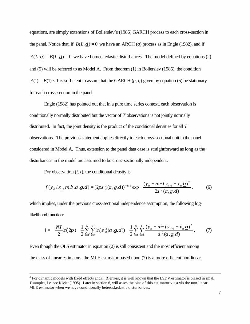
equations, are simply extensions of Bollerslev’s (1986) GARCH process to each cross-section in

the panel. Notice that, if 0),( =δLB we have an ARCH (q) process as in Engle (1982), and if

0),(),( == δγ LBLA we have homoskedastic disturbances. The model defined by equations (2)

and (5) will be referred to as Model A. From theorem (1) in Bollerslev (1986), the condition

1)1()1( <+ BA is sufficient to assure that the GARCH (p, q) given by equation (5) be stationary

for each cross-section in the panel.

Engle (1982) has pointed out that in a pure time series context, each observation is

conditionally normally distributed but the vector of T observations is not jointly normally

distributed. In fact, the joint density is the product of the conditional densities for all T

observations. The previous statement applies directly to each cross-sectional unit in the panel

considered in Model A. Thus, extension to the panel data case is straightforward as long as the

disturbances in the model are assumed to be cross-sectionally independent.

For observation (i, t), the conditional density is:

),,(2

)(exp)),,(2(),,,,,/(

2

212/12

δγασβφµ

δγαπσδγαβµit

itititititit

yyxyf

x−−−−= −− , (6)

which implies, under the previous cross-sectional independence assumption, the following log-

likelihood function:

∑ ∑∑∑= = =

−

=

−−−−−−=

N

i

N

i

T

t it

itititT

tit

yyNTl

1 1 12

21

1

2

),,(

)(

21

)),,(ln(21

)2ln(2 δγασ

βφµδγασπ

x, (7)

Even though the OLS estimator in equation (2) is still consistent and the most efficient among

the class of linear estimators, the MLE estimator based upon (7) is a more efficient non-linear

3 For dynamic models with fixed effects and i.i.d. errors, it is well known that the LSDV estimator is biased in small T samples, i.e. see Kiviet (1995). Later in section 6, will asses the bias of this estimator vis a vis the non-linear MLE estimator when we have conditionally heteroskedastic disturbances.

8

estimator. In addition, by using MLE we can obtain the parameters of both, the conditional

mean (equation 2) and conditional variance (equation 5) simultaneously.4

From MLE theory we know that under regularity conditions the MLE estimator of the

parameter vector )'',',,',( δγαβµθ = is consistent, asymptotically efficient and asymptotically

normally distributed. These excellent asymptotic properties, however do not directly speak to

the properties of the estimator in sample sizes likely to be encountered in practice. We thus

provide some evidence on the finite sample performance of this MLE estimator relative its OLS

counterpart by Monte Carlo simulations for a few designs. We present these results in Section 6

below.

Finally, it is important to notice that our model can be easily extended to the GARCH-M

class of models in which the conditional variance enters into the conditional mean equation and

also to models where exogenous regressors enter the variance equation. In the former case,

equation (2) becomes:

ititititit uyy ++++= − ρσβφµ x1 , Tt K,1= . (8)

In the later case, equation (5) can be reformulated as:

θσδγασ itititit LBuLA z+++= 222 ),(),( , (9)

where itz is a vector of explanatory variables that may or may not include the variables in itx ,

and θ is a vector of parameters.

4 We will pursue direct maximization of (7) by numerical methods as given in the Optimization module of the GAUSS computer program. The asymptotic covariance matrix of the MLE estimator will be approximated as the

9

4. Relaxing the Homogeneity Assumptions

Model A can easily be modified to allow for different forms of parameter heterogeneity.

In principle, it is possible to have heterogeneity in intercepts and/or slopes in both the mean and

variance regressions. In fact there are 16 distinct combinations. In order to have a manageable

number of cases we only allow for heterogeneity in intercepts in the mean and variance

equations. In addition to Model A, we consider the following 3 models:

(i) Individual effects in the mean equation and full parameter homogeneity in the

variance equation (Model B).

(ii) Individual effects in the variance equation and full parameter homogeneity in the

mean equation (Model C)

(iii) Individual effects in both the mean and variance equations (Model D).

The mean and variance equations for Model D are given by

itititiit uyy +++= − βφµ x1 , Ni ,,1 K= , Tt K,1= (10)

222 ),(),( ititiit LBuLA σδγασ ++= , (11)

with iµ and iα representing the corresponding individual specific effects. In this case, the full

parameter vector )'',',',','( δγαβµθ = has )12( ++++ qpkN elements since µ and α are

vectors of dimension N with typical elements iµ and iα respectively. If these individual-

specific effects are treated as fixed, the basic model given in the previous section applies directly

to this case with no modifications other than including dummy variables in both the mean and

variance equations. Model B considers individual effects in the mean equation and a common

intercept coefficient in the variance equation )( αα =i . In this case there are )2( ++++ qpkN

inverse of the outer product of the gradient vectors of l, evaluated at actual MLE estimates.

10

parameters to be estimated. The same number of parameters would have to be estimated in the

case of Model C.

If the cross-section dimension of the sample (N) is not small, however, the number of

parameters to estimate can become unusually large. In this situation it would be convenient to

sweep out the individual effects in the mean equation if they are found significant in order to

reduce the number of parameters to be estimated.

5. Choosing the Correct Panel GARCH model

We propose the following methodology to identify the appropriate statistical model.

First, test for the presence of individual effects in the mean equation. Second, test for ARCH

effects using OLS or LSDV residuals depending on the results in the first step. Third, determine

if there are individual effects in the conditional variance process. Finally, after choosing and

estimating a model, check its residuals to ensure that there is no remaining conditional

heteroskedasticity.

5.1 testing for individual effects in the mean equation

We propose testing for individual effects in the mean equation using the LSDV estimator

with heteroskedasticity and autocorrelation consistent covariance matrix, along the lines of

White (1980) and Newey and West (1987) estimators applied to panel.5

For models A and B, where the variance process is identical across units, the OLS and

LSDV are still best linear estimators. However for models C and D the unconditional variance

will be different across units and the previous estimators will no longer be efficient and inference

based upon them will not be valid. Given that we do not know a priori which is the appropriate

11

model and that we can have auto correlation problems in practice, it seems convenient to use a

covariance matrix robust to heteroskedasticity and autocorrelation. Specifically we will test the

null hypothesis NH µµµ === L210 : by means of a Wald-test, which will follow a 2)1( −Nχ

distribution asymptotically.

5.2 testing for ARCH effects and individual effects in the conditional variance

The second step uses either LSDV or OLS squared residuals (according to whether

individual effects were found or not in the mean equation) to test for ARCH effects. We can use

the estimated autocorrelation and / or partial autocorrelation coefficients to determine the

existence and possible order of ARCH effects. Also, the null hypothesis of conditional

homoskedasticity or ARCH (0), against ARCH (j) can be tested for a few relevant values of j.

This can be done via LM-test statistics based on the previous squared residuals and referred to

the 2)( jχ distribution. In practice, rejecting ARCH(0) in favor of a large number of significant

lags will lead to the estimation of a GARCH model. That is to say, we are testing for ARCH, but

given that a GARCH(1,1) approximates quite well ARCH models of arbitrarily large orders, we

are considering here as viable alternatives ARCH(1), ARCH(2), and GARCH(1,1).

Finally, we test for individual effects in the ARCH process in two ways. First we can test

whether the squared residuals have a constant mean across the cross-sectional units. Second, we

can regress the OLS/LSDV squared residuals on an appropriate number of lagged squared

residuals with and without individual effects and compare the fits via an F or Chi-square test.

5 Arellano (1987) has extended the White’s heteroskedasticity consistent covariance estimator to panel data but this estimator is not apropriate here since it has been formulated for small T and large N panels which is not our case.

12

5.3 selecting the final model

After initially choosing an appropriate conditional variance model, based on an analysis

of the squared residuals described above, and estimating the full model via maximum likelihood,

it is important to make sure that all conditional heteroskedasticty has been captured in the

estimation. We can accomplish this in two ways. First, we can add additional ARCH or GARCH

terms and check their significance. Second, we can test the squared normalized residuals for any

autocorrelation pattern. If significant patterns remain, alternative specifications of the

conditional variance should be estimated and checked.

6. Finite Sample Performance of the Panel GARCH Estimator

It is well known that in the context of time series GARCH models, the (non-linear) MLE

estimator not only has desirable asymptotic properties but also it is more efficient than the OLS

estimator. Little is known, however, on the finite sample performance of the MLE estimator

relative to its OLS counterpart in finite samples, particularly in panel data. This section presents

some Monte Carlo results that shed light on the performance of the MLE estimator in panels with

GARCH errors. In particular, we study the bias and precision of the MLE and OLS estimators of

the parameters of the conditional mean equation (equation 2) as well as the performance of the

MLE estimator of the parameters in the variance equation (equation 4).

6.1 Monte Carlo design

The data-generating model is defined by equation (2) and equation (4) given before.

Notice that the error term in the mean equation is drawn from a normal distribution with mean

zero and a variance that changes over time according to equation (4). For practical purposes the

13

simulation study is limited to the pooled regression model and to the cases of ARCH (1) and

GARCH (1,1) errors.

For the conditional mean, we consider separately the static and dynamic cases. In the

static case, only one exogenous regressor with coefficient 1=β enters the mean equation. In the

dynamic case, we consider a pure AR (1) process without exogenous regressors. In this case, the

AR parameter φ takes the alternative values {0.5, 0.8}, representing moderate and high

persistence of the AR (1) process respectively. The intercepts of the mean and variance

equations are each set to 1.0 in all cases ( 1==αµ ). For the ARCH (1) process, 1γ (the

coefficient of 21−tu ) takes on the alternative values {0.5, 0.9}, representing moderate and high

degrees of conditional heteroskedasticity. For the GARCH (1,1) process, we set 3.01 =γ (the

coefficient on the term 21−tu ) for all cases, but we allow 1δ (the coefficient on the term 2

1−tσ ) to

take on the values {0.3, 0.6,}.

Finally, we have set the number of trials in each Monte Carlo experiment to 1000 but

given that the program that solves the model numerically does not always converge, the final

number of (valid) trials is sometimes less than 1000. The results are presented in Tables A1

through A8 in the Appendix.

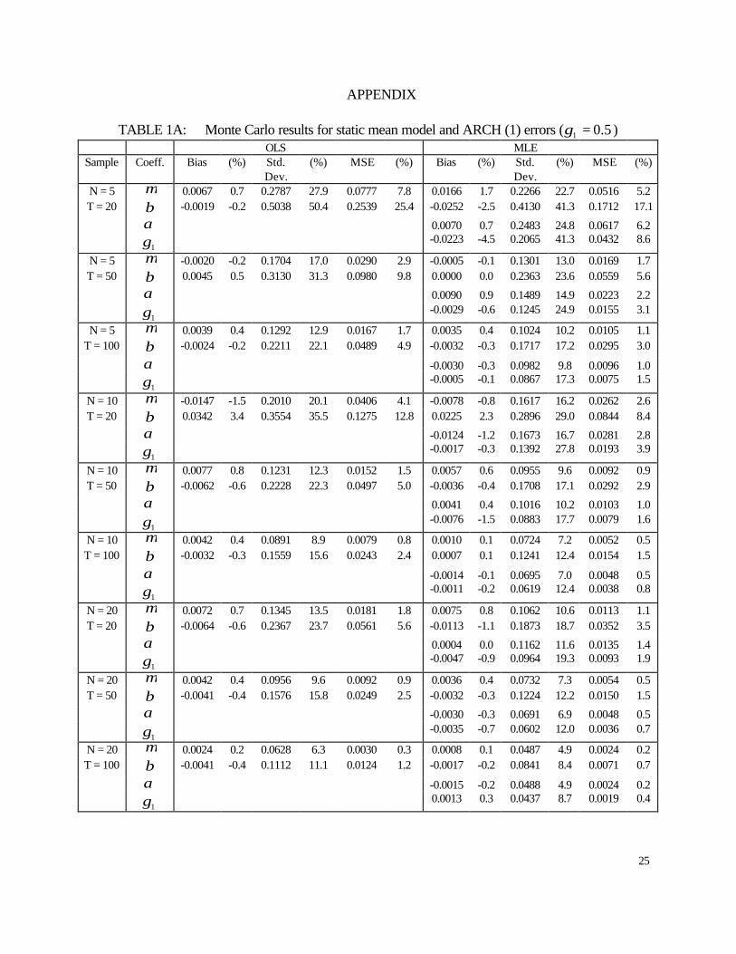
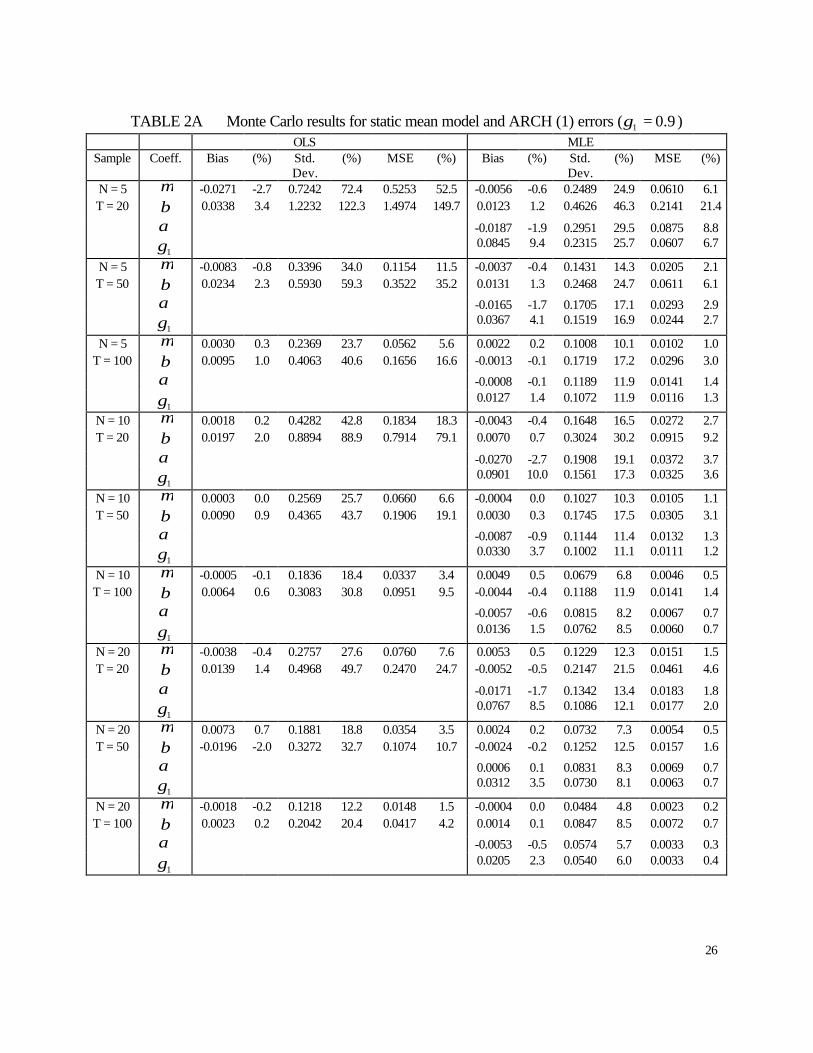
6.2 static panel ARCH results

Tables A1 and A2 contain the results for the static mean, ARCH(1), case. The first

observation is that as T increases for a given N, the OLS and MLE estimators of the intercept and

slope coefficients in the mean equation improve on a mean squared error criterion. Although we

do not observe a clear pattern in the bias of both estimators, their standard errors clearly diminish

with T. Second, when comparing the OLS and MLE estimators (for the mean equation), we find

14

that the MLE outperforms the OLS estimator in terms of precision and mean squared error. In

fact the MLE estimator consistently has a MSE of about half of that of the OLS estimator in the

case 5.01 =γ , and less than half in the case 9.01 =γ .

Turning to the MLE estimator of the variance coefficients α and 1γ (intercept and ARCH

(1) coefficient respectively), in both cases we observe improvements in precision and mean

squared error as T increases. However, there is no obvious pattern in the biases. On a mean

squared error criterion, the MLE estimator of the variance coefficients appears to be quite

acceptable.

Turning back to the mean equation, it is worth mentioning that although the MLE

estimator is better than its OLS counterpart, the MLE estimator of the intercept coefficient still

shows relatively large mean squared errors as percentage of the true parameter values. In fact, in

the case of the smallest sample (N=5, T=20) the mean squared error of this estimator 17.1% and

21.4% for the cases of 9.0,5.01 =γ respectively.

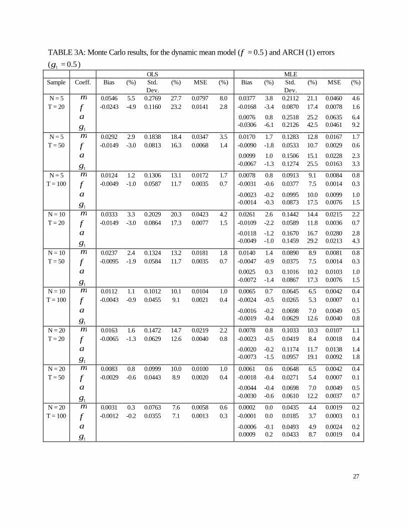
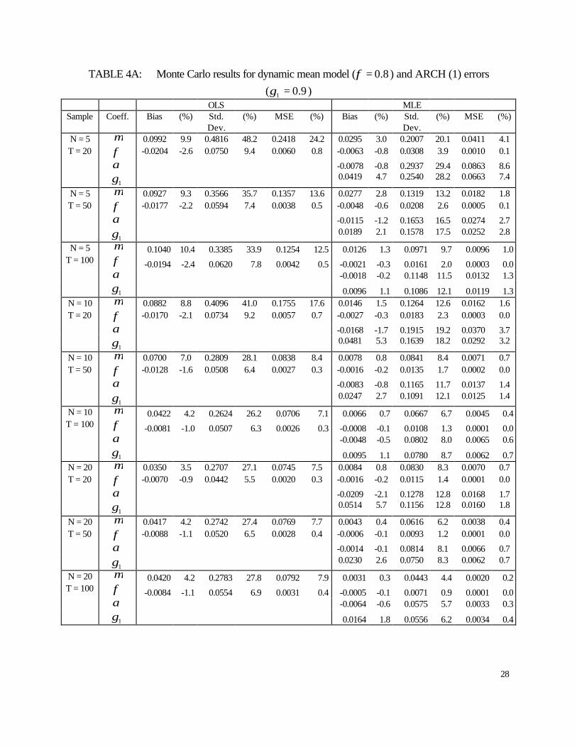
6.3 dynamic panel ARCH results

Tables A3 and A4 show the results for the ARCH (1) process in the dynamic mean case.

We find that both the OLS and MLE estimators of the coefficients of the (dynamic) mean

equation become more precise as T increases. Overall, both estimators improve as T increases

showing smaller mean squared errors in all cases. As opposed to our findings in the static case,

in this case we observe that the MLE estimator of the intercept and AR parameters in the mean

equation clearly outperforms the OLS estimator in terms of both bias and precision.

Regarding the MLE estimators of the ARCH equation, we find that their precision

increases with the sample size and that the biases generally become smaller as T increases. On a

15

mean squared error criterion, we find improvement in the MLE estimators of both parameters (α

and 1γ ) as the sample size increases in all cases.

When looking at the performance of these estimators as the persistence of the mean

process as well as the strength of the ARCH process increase, given the sample sizes, we observe

that the biases of the coefficients of the variance equation generally increase. Also, the bias of α

becomes negative while the bias of 1γ becomes positive. Another pattern that we find is that the

standard error of α increases while the standard error of 1γ decreases. Overall, on a mean

squared error criterion, we find that the results for the MLE estimator of the variance equation

are quite acceptable.

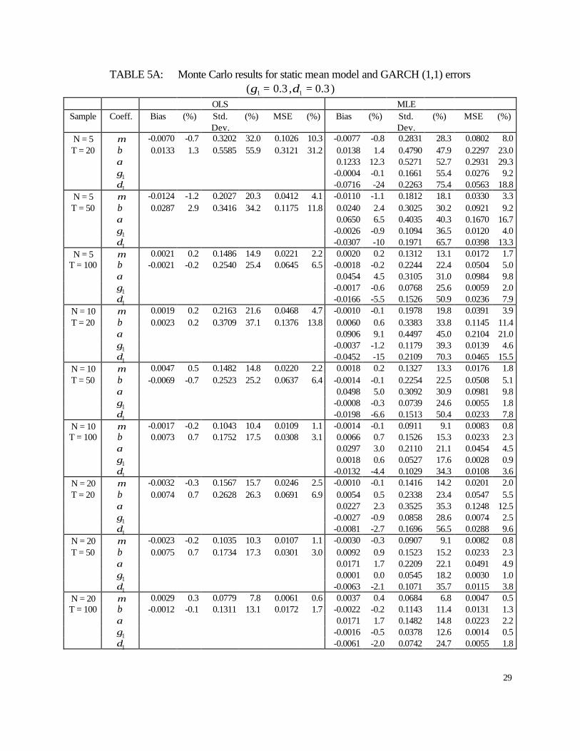
6.4 static Panel GARCH results

Monte Carlo results for the static mean case with GARCH errors are presented in Tables

A5 and A6. We observe that the MLE and OLS estimators of the coefficients of the mean

equation ( µ and β ) improve as T increases in terms of standard errors and mean squared errors.

Also the MLE estimators of the previous coefficients are less biased than their OLS counterparts

in most cases. In terms of precision, the MLE estimators outperform the OLS estimators in all

cases. A similar result is found in terms of mean squared errors.

Concerning the MLE estimators of the coefficients in the variance equation ( 11 ,, δγα ),

we find that their biases generally diminish as T increases. Similar results are found for the

standard errors and mean squared errors.

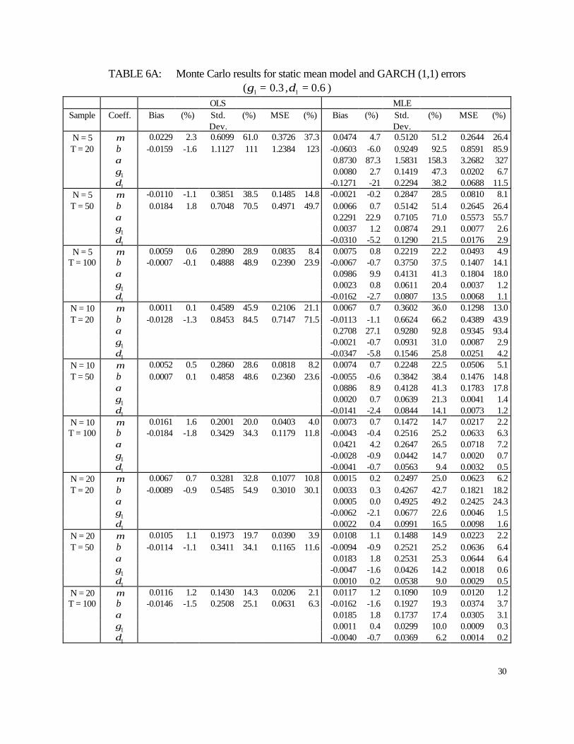
When the persistence of the GARCH process is increased, the performance of OLS and

MLE estimators of the mean coefficients worsens in terms of bias and precision, although the

MLE is still better than the OLS estimator. Regarding the MLE estimator of the variance

16

coefficients we observe that the bias increases except for the GARCH coefficient ( 1δ ). On the

other hand, the ARCH and GARCH coefficients improve in terms of dispersion. On a mean

squared error criterion, the estimators of these two coefficients improve while the estimator of

the intercept coefficient worsens.

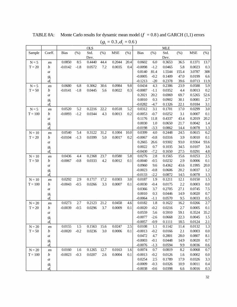
6.5 dynamic Panel GARCH results

The Monte Carlo results for the model with dynamic mean and GARCH (1,1) errors are

presented in Tables A7 and A8. In this case we find that the MLE and OLS estimators of the

parameters in the mean equation ( µ and φ) improve as T increases given N on any criterion

considered. When comparing both estimators we find that in all cases the MLE estimator is less

biased and more precise than the OLS estimator.

For the MLE estimators of the variance coefficients, except for the ARCH parameter

( 1δ ), we find that they are generally less biased as T increases. Also, all MLE estimators of the

variance coefficients perform better both in terms of standard errors and mean squared errors as

T increases in all cases considered.

When we allow for more persistence in both the dynamic mean and variance processes,

we find that for both the OLS and MLE estimators of the mean equation, the bias of the intercept

coefficient ( µ) increases while the bias of the slope coefficient (φ) decreases. The same pattern

is observed in terms of dispersion. In this case we observe again that the MLE outperforms the

OLS estimator. Regarding the MLE estimators of the variance coefficients, we find that the

intercept coefficient worsens but the ARCH and GARCH coefficients improve on a mean

squared error. In fact, the intercept becomes more biased and less precise while the ARCH and

GARCH coefficients become less biased and more precise. Overall, as the values of φ and 1δ

17

coefficients are increased we obtain less reliable estimators of the intercepts in both the mean

and variance equations. However, the estimators of the slope coefficients in the mean (φ) and

variance equations ( 11 ,δγ ) become more reliable.

7. Empirical Examples

In this section we illustrate the applicability of the panel GARCH estimation and testing

methodology proposed in section 5. Specifically we investigate whether the uncertainty

associated with investment in a panel of five large U.S. manufacturing firms, and inflation in a

panel of seven Latin American countries can in fact be captured with ARCH or GARCH models.

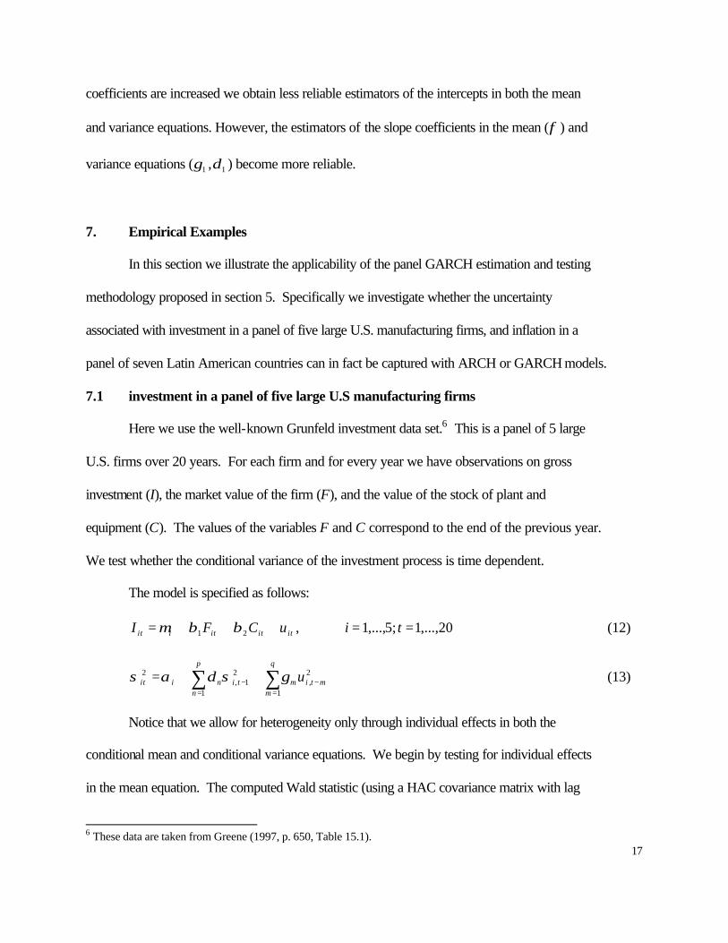
7.1 investment in a panel of five large U.S manufacturing firms

Here we use the well-known Grunfeld investment data set.6 This is a panel of 5 large

U.S. firms over 20 years. For each firm and for every year we have observations on gross

investment (I), the market value of the firm (F), and the value of the stock of plant and

equipment (C). The values of the variables F and C correspond to the end of the previous year.

We test whether the conditional variance of the investment process is time dependent.

The model is specified as follows:

itititiit uCFI +++= 21 ββµ , 20,...,1;5,...,1 == ti (12)

∑∑=

−=

− ++=q

mmtim

p

ntiniit u

1

2,

1

21,

2 γσδασ (13)

Notice that we allow for heterogeneity only through individual effects in both the

conditional mean and conditional variance equations. We begin by testing for individual effects

in the mean equation. The computed Wald statistic (using a HAC covariance matrix with lag

6 These data are taken from Greene (1997, p. 650, Table 15.1).

18

truncation equal to 2), is 226.1182)4( =χ , which ishigh enough to clearly reject the null

hypothesis of no individual effects in the mean equation. Next we attempt to identify ARCH

effects using the squared residuals from LSDV estimation of the mean equationWe compute the

partial auto correlation coefficients of the squared residuals (Table 1).

TABLE 1: Estimated partial auto-correlation coefficients on squared LSDV residuals (investment data)

Coefficient t-ratio p-value

PAC(1) 0.5225* 4.0785 0.0000 PAC(2) -0.0925 -0.6633 0.7455 PAC(3) 0.0519 0.3542 0.3621

PAC(4) 0.0728 0.4862 0.3139 PAC(5) 0.2325° 1.5168 0.0664 PAC(6) -0.1235 -0.7816 0.7817 PAC(7) 0.1293 0.7731 0.2207 PAC(8) 0.0482 0.2828 0.3889 PAC(9) 0.1245 0.6978 0.2435

PAC(10) -0.1638 -0.9763 0.8342 LSDV estimated squared residuals are used since there is evidence of individual effects in the mean equation. The symbols *, ^ and ° indicate respectively 1%, 5% and 10% significance levels.

In these data, only the first partial autocorrelation coefficient is statistically significant at

the 0.05 level. It thus appears that the conditional variance of the error process follows an

ARCH(1). Next, we try to determine if the conditional variance equation has individual effects

by regressing the LSDV squared residuals on their first lag and a set of firm specific intercepts

and then testing whether the intercepts share a common coefficient.

The computed statistics 960.2)94,4( =F and 864.112)4( =χ reject the null hypothesis of no

individual effects in the ARCH process at the 5% significance level. The model selection

process thus suggests that there are individual effects in the mean equation, and that the

conditional variance follows an ARCH (1) with individual effects, which is our model D in

section V above.

19

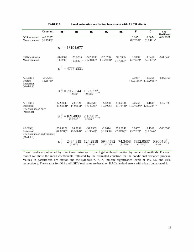
TABLE 2: Panel estimation results for Investment with ARCH effects

Constant µµ 1 µµ 2 µµ 3 µµ 4 µµ 5 F C Log-likelihood

OLS estimates -48.0297 0.1051 0.3054 -624.9927 Mean equation (-2.1903)^ (8.2850)* (3.8471)*

677.161942 =σ LSDV estimates -76.0668 -29.3736 -242.1708 -57.8994 92.5385 0.1060 0.3467 -561.8468 Mean equation (-0.7990) (-1.8587)° (-5.0185)* (-3.2350)* (1.7389)° (4.7937)* (7.1857)*

2951.47772 =σ ARCH(1): -37.4254 0.1087 0.3358 -584.8165 Pooled (-6.6876)* (40.3168)* (15.2096)* Regression (Model A)

2

1)^9566.2()5385.1(

2 ˆ5593.16344.796 −°

+= tt uσ

ARCH(1): 222.2649 20.6421 -82.6617 -4.8258 230.9331 0.0502 0.1699 -510.6109 Individual (11.6958)* (4.9555)* (-6.4023)* (-0.9006) (21.7843)* (10.4699)* (20.0284)* Effects in mean only (Model B)

2

1*)3285.5(*)0355.3(

2 ˆ1890.24899.109 −+= tt uσ

ARCH(1): 256.4222 24.7232 -51.7389 -0.2614 275.3949 0.0457 0.1518 -503.6508 Individual (8.3794)* (3.5760)* (-1.9547)^ (-0.0368) (7.8697)* (3.7677)* (3.0724)* Effects in mean and variance (Model D)

2

1*)8303.2()^0791.2()^1779.2(*)5735.2()^8053.1()9555.0(

2 ˆ9004.00537.58523458.744582.5942918.124819.2434 −+++++= tt uσ

These results are obtained by direct maximization of the log-likelihood function by numerical methods. For each model we show the mean coefficients followed by the estimated equation for the conditional variance process. Values in parenthesis are t-ratios and the symbols *, ^, °, indicate significance levels of 1%, 5% and 10% respectively. The t-ratios for OLS and LSDV estimates are based on HAC standard errors with a lag truncation of 2.

20

Table 2 presents maximum likelihood estimates of this model. For comparison we also

consider Model A, which corresponds to a pooled regression model whose conditional variance

follows an ARCH(1) process, and present OLS and LSDV estimates of the mean equation.

As noted above, the data reject the null hypothesis of no individual effects in the mean

equation at the 0.01 level. This can be seen in Table 2 either by comparing either panels one and

two (OLS vs. LSDV) or by comparing panels three and four (ARCH(1) pooled vs. ARCH(1)

with individual mean effects). The data also reject the null hypothesis of conditional

homoskedasticity, also at the 0.01 level. This can be seen either by comparing panels one and

three (OLS vs. ARCH(1) pooled), or panels two and four (LSDV vs. ARCH(1) with individual

mean effects) in Table 2. Finally the data reject the null hypothesis of no individual effects in

the conditional variance equation at the 0.01 level (as seen by comparing panels 4 and 5 in Table

2). The final preferred model is still Model D, the final estimation in Table 2, which can be

described as ARCH(1) with individual effects in both the mean and conditional variance

equations. We do not find evidence of any significant auto-correlation in the normalized squared

residuals from Model D, thus ensuring that this specification captures all conditional

heteroskedasticity from these data.

From the reported results, we can see that accounting for the conditional

heteroskedasticity in data notably changes the values of the coefficients on the explanatory

variables in the mean equation. The coefficients on C (value of the firm’s plant and equipment)

and F (the firm’s market capitalization) are both around 50% smaller and have smaller t-statistics

in the preferred model than in the OLS, LSDV or ARCH(1) pooled specifications, though both

21

coefficients are still significant at the 0.01 level.7 In sum we find significant conditional

heteroskedasticity in this well-known panel, and modeling it via panel GARCH materially

affects the results of interest.

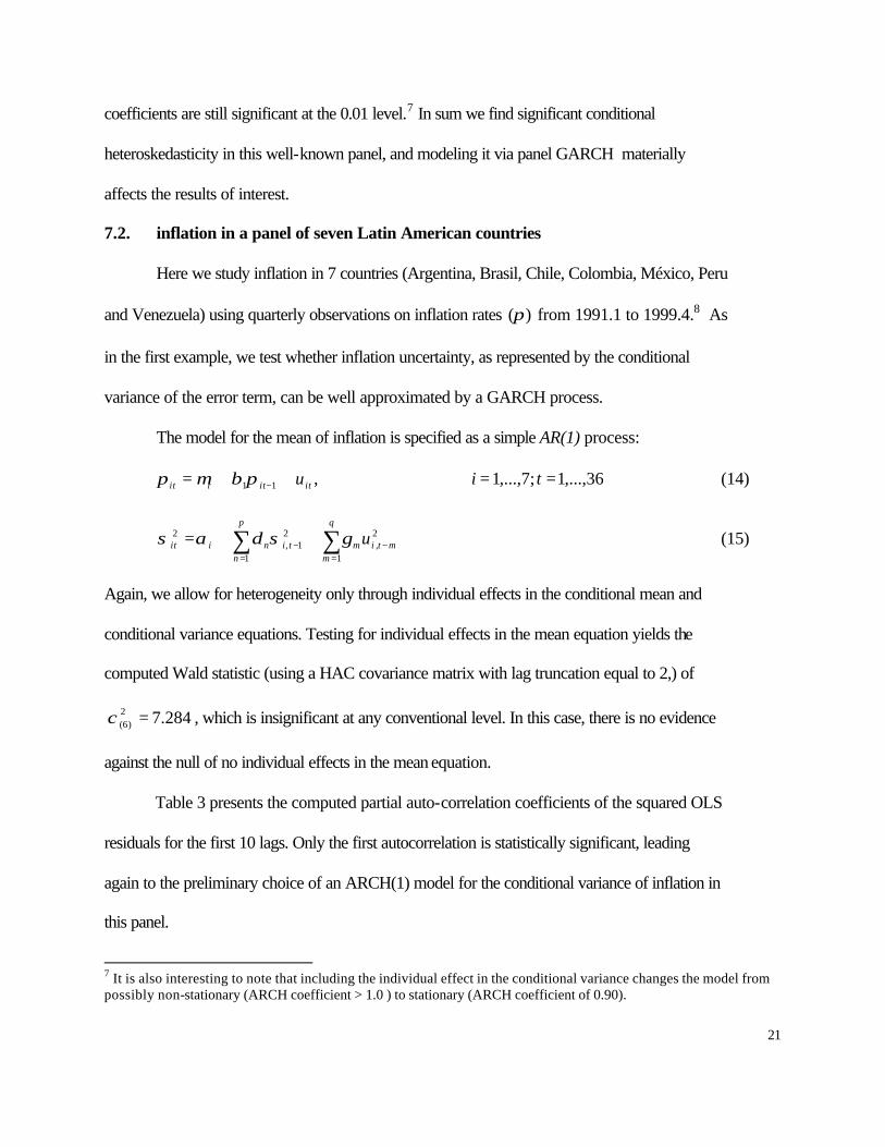
7.2. inflation in a panel of seven Latin American countries

Here we study inflation in 7 countries (Argentina, Brasil, Chile, Colombia, México, Peru

and Venezuela) using quarterly observations on inflation rates )(π from 1991.1 to 1999.4.8 As

in the first example, we test whether inflation uncertainty, as represented by the conditional

variance of the error term, can be well approximated by a GARCH process.

The model for the mean of inflation is specified as a simple AR(1) process:

ititiit u++= −11πβµπ , 36,...,1;7,...,1 == ti (14)

∑∑=

−=

− ++=q

mmtim

p

ntiniit u

1

2,

1

21,

2 γσδασ (15)

Again, we allow for heterogeneity only through individual effects in the conditional mean and

conditional variance equations. Testing for individual effects in the mean equation yields the

computed Wald statistic (using a HAC covariance matrix with lag truncation equal to 2,) of

284.72)6( =χ , which is insignificant at any conventional level. In this case, there is no evidence

against the null of no individual effects in the mean equation.

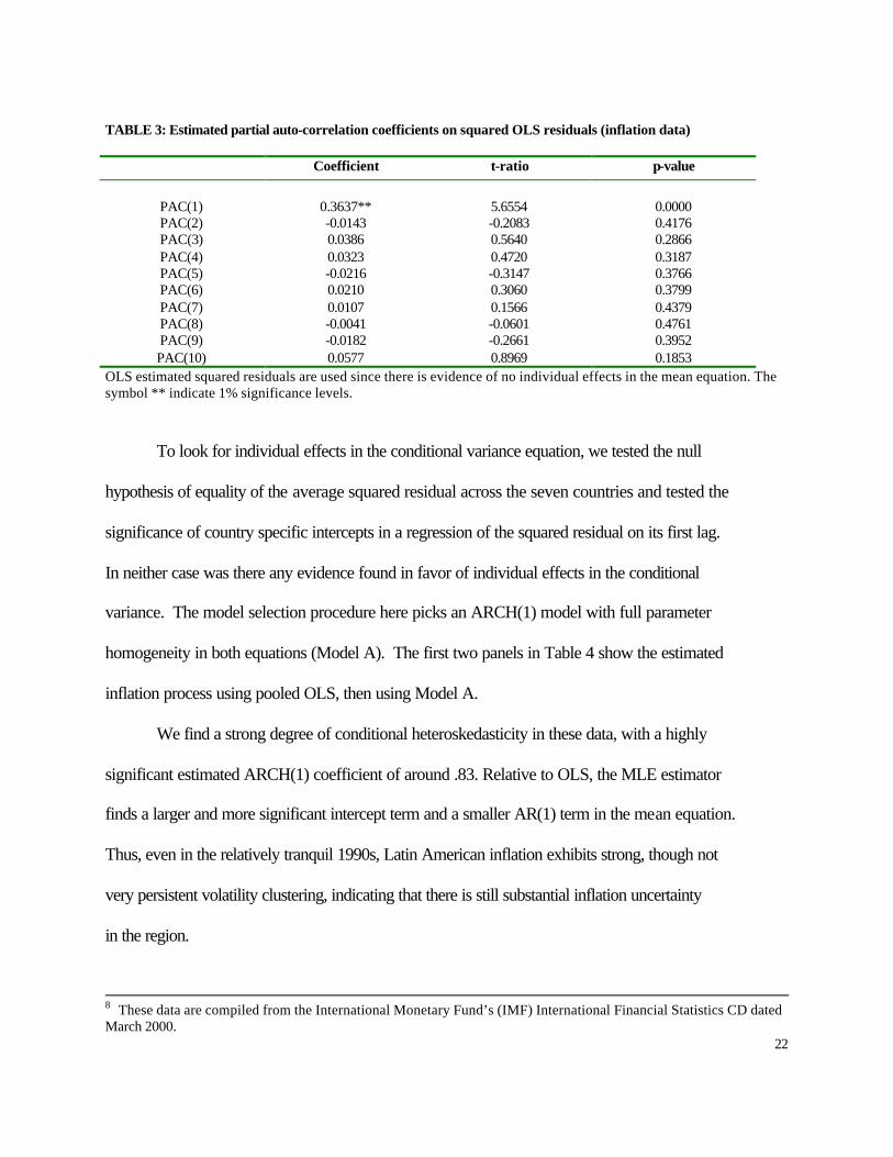
Table 3 presents the computed partial auto-correlation coefficients of the squared OLS

residuals for the first 10 lags. Only the first autocorrelation is statistically significant, leading

again to the preliminary choice of an ARCH(1) model for the conditional variance of inflation in

this panel.

7 It is also interesting to note that including the individual effect in the conditional variance changes the model from possibly non-stationary (ARCH coefficient > 1.0 ) to stationary (ARCH coefficient of 0.90).

22

TABLE 3: Estimated partial auto-correlation coefficients on squared OLS residuals (inflation data)

Coefficient t-ratio p-value

PAC(1) 0.3637** 5.6554 0.0000 PAC(2) -0.0143 -0.2083 0.4176 PAC(3) 0.0386 0.5640 0.2866 PAC(4) 0.0323 0.4720 0.3187 PAC(5) -0.0216 -0.3147 0.3766 PAC(6) 0.0210 0.3060 0.3799 PAC(7) 0.0107 0.1566 0.4379 PAC(8) -0.0041 -0.0601 0.4761 PAC(9) -0.0182 -0.2661 0.3952 PAC(10) 0.0577 0.8969 0.1853

OLS estimated squared residuals are used since there is evidence of no individual effects in the mean equation. The symbol ** indicate 1% significance levels.

To look for individual effects in the conditional variance equation, we tested the null

hypothesis of equality of the average squared residual across the seven countries and tested the

significance of country specific intercepts in a regression of the squared residual on its first lag.

In neither case was there any evidence found in favor of individual effects in the conditional

variance. The model selection procedure here picks an ARCH(1) model with full parameter

homogeneity in both equations (Model A). The first two panels in Table 4 show the estimated

inflation process using pooled OLS, then using Model A.

We find a strong degree of conditional heteroskedasticity in these data, with a highly

significant estimated ARCH(1) coefficient of around .83. Relative to OLS, the MLE estimator

finds a larger and more significant intercept term and a smaller AR(1) term in the mean equation.

Thus, even in the relatively tranquil 1990s, Latin American inflation exhibits strong, though not

very persistent volatility clustering, indicating that there is still substantial inflation uncertainty

in the region.

8 These data are compiled from the International Monetary Fund’s (IMF) International Financial Statistics CD dated March 2000.

23

TABLE 4: Panel estimation results for Inflation with ARCH effects

constant ππt-1 Log-likelihood

1.0392 (0.5216)

0.9065 (9.4187)*

-1156.3338 OLS estimates Mean equation

974.5702 =σ

1.8356 (3.3807)*

0.8195 (37.2695)*

-926.1028 ARCH(1): Pooled regression

(Model A) 2

1)*1209.6()*1457.8(

2 ˆ8297.02354.36 −+= tt uσ

1.5561

(3.33960)* 0.8368

(29.2266)*

-904.5676 ARCH(1): Pooled regression

(Model A with lagged inflation in

variance)

1*)6897.5(

21

*)0020.4(*)0068.4(

2 4664.2ˆ4091.08704.9 −− ++= ttt u πσ

These results have been obtained by direct maximization of the log-likelihood function by numerical methods. For each model we show the mean coefficients followed by the estimated variance or the estimated equation for the conditional variance process. Values in parenthesis are t-ratios and the symbol (*) indicates significance level of 1%. The t-ratios for OLS estimates are based on HAC standard errors with a lag truncation of 2.

7.3. is higher inflation less predictable in this panel?

Friedman (1977) and Ball (1992) argue that higher average inflation rates are less

predictable than lower rates. Here we test that hypothesis with our 7 country panel, using a

simple modification of our panel GARCH estimator. Specifically, we include lagged inflation

as a regressor in the ARCH equation. The results appear in the last panel of Table 4 where the

lagged inflation variable is positive and significant.9 Compared to the standard panel ARCH(1)

estimates in the middle panel, we find that the ARCH coefficient falls from around .8 to around

.4, the intercept in the conditional variance equation falls from around 36 to around 10, and the

maximized value of the likelihood function rises from –926 to –904.

24

8. Conclusions

In this paper, we present and implement a methodology to test for and estimate GARCH

effects in panel data sets. Our statistical method consists of the following steps: (i) Testing for

individual effects in the mean equation. (ii) Testing for ARCH effects using squared LSDV or

OLS residuals (depending on whether individual effects are found or not in the previous stage),

and testing for the presence of individual effects in the ARCH process. (iii) Estimating the

relevant GARCH specification by maximum likelihood and checking the squared residuals.

We present Monte Carlo results showing that the MLE estimator of the coefficients of the

mean equation is less biased and more precise relative to their OLS counterpart in practically all

cases considered. Also we find that the MLE estimator of the conditional variance coefficients

have a quite acceptable performance except for the intercept in the dynamic mean cases with

high persistence of the variance process.

Our empirical applications show that the uncertainty associated with investment decisions

(in the panel of 5 large U.S. manufacturing firms) as well as inflation (in the panel of 7 Latin

American countries), can be well approximated by a pooled conditionally heteroskedastic error

process. Our results show that accounting for this volatility clustering in the data can materially

change the estimated effects of variables of interest.

Straightforward, but important, extensions of this work include panel GARCH-M models

where the effects of uncertainty on the conditional mean can be tested, and the further

development of panel GARCH models with exogenous variables in the conditional variance

equation.

9 It should be remarked that all the parameters of the model (mean and variance) are estimated simultaneously by Maximum Likelihood. Also, for the two ARCH estimations presented here, we have not found evidence of any significant auto correlation when examining their corresponding squared normalized residuals.

25

APPENDIX

TABLE 1A: Monte Carlo results for static mean model and ARCH (1) errors ( 5.01 =γ ) OLS MLE

Sample Coeff. Bias (%) Std. Dev.

(%) MSE (%) Bias (%) Std. Dev.

(%) MSE (%)

N = 5 µ 0.0067 0.7 0.2787 27.9 0.0777 7.8 0.0166 1.7 0.2266 22.7 0.0516 5.2 T = 20 β -0.0019 -0.2 0.5038 50.4 0.2539 25.4 -0.0252 -2.5 0.4130 41.3 0.1712 17.1

α 0.0070 0.7 0.2483 24.8 0.0617 6.2

1γ -0.0223 -4.5 0.2065 41.3 0.0432 8.6

N = 5 µ -0.0020 -0.2 0.1704 17.0 0.0290 2.9 -0.0005 -0.1 0.1301 13.0 0.0169 1.7 T = 50 β 0.0045 0.5 0.3130 31.3 0.0980 9.8 0.0000 0.0 0.2363 23.6 0.0559 5.6

α 0.0090 0.9 0.1489 14.9 0.0223 2.2

1γ -0.0029 -0.6 0.1245 24.9 0.0155 3.1

N = 5 µ 0.0039 0.4 0.1292 12.9 0.0167 1.7 0.0035 0.4 0.1024 10.2 0.0105 1.1 T = 100 β -0.0024 -0.2 0.2211 22.1 0.0489 4.9 -0.0032 -0.3 0.1717 17.2 0.0295 3.0

α -0.0030 -0.3 0.0982 9.8 0.0096 1.0

1γ -0.0005 -0.1 0.0867 17.3 0.0075 1.5

N = 10 µ -0.0147 -1.5 0.2010 20.1 0.0406 4.1 -0.0078 -0.8 0.1617 16.2 0.0262 2.6 T = 20 β 0.0342 3.4 0.3554 35.5 0.1275 12.8 0.0225 2.3 0.2896 29.0 0.0844 8.4

α -0.0124 -1.2 0.1673 16.7 0.0281 2.8

1γ -0.0017 -0.3 0.1392 27.8 0.0193 3.9

N = 10 µ 0.0077 0.8 0.1231 12.3 0.0152 1.5 0.0057 0.6 0.0955 9.6 0.0092 0.9 T = 50 β -0.0062 -0.6 0.2228 22.3 0.0497 5.0 -0.0036 -0.4 0.1708 17.1 0.0292 2.9

α 0.0041 0.4 0.1016 10.2 0.0103 1.0

1γ -0.0076 -1.5 0.0883 17.7 0.0079 1.6

N = 10 µ 0.0042 0.4 0.0891 8.9 0.0079 0.8 0.0010 0.1 0.0724 7.2 0.0052 0.5 T = 100 β -0.0032 -0.3 0.1559 15.6 0.0243 2.4 0.0007 0.1 0.1241 12.4 0.0154 1.5

α -0.0014 -0.1 0.0695 7.0 0.0048 0.5

1γ -0.0011 -0.2 0.0619 12.4 0.0038 0.8

N = 20 µ 0.0072 0.7 0.1345 13.5 0.0181 1.8 0.0075 0.8 0.1062 10.6 0.0113 1.1 T = 20 β -0.0064 -0.6 0.2367 23.7 0.0561 5.6 -0.0113 -1.1 0.1873 18.7 0.0352 3.5

α 0.0004 0.0 0.1162 11.6 0.0135 1.4

1γ -0.0047 -0.9 0.0964 19.3 0.0093 1.9

N = 20 µ 0.0042 0.4 0.0956 9.6 0.0092 0.9 0.0036 0.4 0.0732 7.3 0.0054 0.5 T = 50 β -0.0041 -0.4 0.1576 15.8 0.0249 2.5 -0.0032 -0.3 0.1224 12.2 0.0150 1.5

α -0.0030 -0.3 0.0691 6.9 0.0048 0.5

1γ -0.0035 -0.7 0.0602 12.0 0.0036 0.7

N = 20 µ 0.0024 0.2 0.0628 6.3 0.0030 0.3 0.0008 0.1 0.0487 4.9 0.0024 0.2 T = 100 β -0.0041 -0.4 0.1112 11.1 0.0124 1.2 -0.0017 -0.2 0.0841 8.4 0.0071 0.7

α -0.0015 -0.2 0.0488 4.9 0.0024 0.2

1γ 0.0013 0.3 0.0437 8.7 0.0019 0.4

26

TABLE 2A Monte Carlo results for static mean model and ARCH (1) errors ( 9.01 =γ )

OLS MLE Sample Coeff. Bias (%) Std.

Dev. (%) MSE (%) Bias (%) Std.

Dev. (%) MSE (%)

N = 5 µ -0.0271 -2.7 0.7242 72.4 0.5253 52.5 -0.0056 -0.6 0.2489 24.9 0.0610 6.1 T = 20 β 0.0338 3.4 1.2232 122.3 1.4974 149.7 0.0123 1.2 0.4626 46.3 0.2141 21.4

α -0.0187 -1.9 0.2951 29.5 0.0875 8.8

1γ 0.0845 9.4 0.2315 25.7 0.0607 6.7

N = 5 µ -0.0083 -0.8 0.3396 34.0 0.1154 11.5 -0.0037 -0.4 0.1431 14.3 0.0205 2.1 T = 50 β 0.0234 2.3 0.5930 59.3 0.3522 35.2 0.0131 1.3 0.2468 24.7 0.0611 6.1

α -0.0165 -1.7 0.1705 17.1 0.0293 2.9

1γ 0.0367 4.1 0.1519 16.9 0.0244 2.7

N = 5 µ 0.0030 0.3 0.2369 23.7 0.0562 5.6 0.0022 0.2 0.1008 10.1 0.0102 1.0 T = 100 β 0.0095 1.0 0.4063 40.6 0.1656 16.6 -0.0013 -0.1 0.1719 17.2 0.0296 3.0

α -0.0008 -0.1 0.1189 11.9 0.0141 1.4

1γ 0.0127 1.4 0.1072 11.9 0.0116 1.3

N = 10 µ 0.0018 0.2 0.4282 42.8 0.1834 18.3 -0.0043 -0.4 0.1648 16.5 0.0272 2.7 T = 20 β 0.0197 2.0 0.8894 88.9 0.7914 79.1 0.0070 0.7 0.3024 30.2 0.0915 9.2

α -0.0270 -2.7 0.1908 19.1 0.0372 3.7

1γ 0.0901 10.0 0.1561 17.3 0.0325 3.6

N = 10 µ 0.0003 0.0 0.2569 25.7 0.0660 6.6 -0.0004 0.0 0.1027 10.3 0.0105 1.1 T = 50 β 0.0090 0.9 0.4365 43.7 0.1906 19.1 0.0030 0.3 0.1745 17.5 0.0305 3.1

α -0.0087 -0.9 0.1144 11.4 0.0132 1.3

1γ 0.0330 3.7 0.1002 11.1 0.0111 1.2

N = 10 µ -0.0005 -0.1 0.1836 18.4 0.0337 3.4 0.0049 0.5 0.0679 6.8 0.0046 0.5 T = 100 β 0.0064 0.6 0.3083 30.8 0.0951 9.5 -0.0044 -0.4 0.1188 11.9 0.0141 1.4

α -0.0057 -0.6 0.0815 8.2 0.0067 0.7

1γ 0.0136 1.5 0.0762 8.5 0.0060 0.7

N = 20 µ -0.0038 -0.4 0.2757 27.6 0.0760 7.6 0.0053 0.5 0.1229 12.3 0.0151 1.5 T = 20 β 0.0139 1.4 0.4968 49.7 0.2470 24.7 -0.0052 -0.5 0.2147 21.5 0.0461 4.6

α -0.0171 -1.7 0.1342 13.4 0.0183 1.8

1γ 0.0767 8.5 0.1086 12.1 0.0177 2.0

N = 20 µ 0.0073 0.7 0.1881 18.8 0.0354 3.5 0.0024 0.2 0.0732 7.3 0.0054 0.5 T = 50 β -0.0196 -2.0 0.3272 32.7 0.1074 10.7 -0.0024 -0.2 0.1252 12.5 0.0157 1.6

α 0.0006 0.1 0.0831 8.3 0.0069 0.7

1γ 0.0312 3.5 0.0730 8.1 0.0063 0.7

N = 20 µ -0.0018 -0.2 0.1218 12.2 0.0148 1.5 -0.0004 0.0 0.0484 4.8 0.0023 0.2 T = 100 β 0.0023 0.2 0.2042 20.4 0.0417 4.2 0.0014 0.1 0.0847 8.5 0.0072 0.7

α -0.0053 -0.5 0.0574 5.7 0.0033 0.3

1γ 0.0205 2.3 0.0540 6.0 0.0033 0.4

27

TABLE 3A: Monte Carlo results, for the dynamic mean model ( 5.0=φ ) and ARCH (1) errors

( 5.01 =γ ) OLS MLE

Sample Coeff. Bias (%) Std. Dev.

(%) MSE (%) Bias (%) Std. Dev.

(%) MSE (%)

N = 5 µ 0.0546 5.5 0.2769 27.7 0.0797 8.0 0.0377 3.8 0.2112 21.1 0.0460 4.6 T = 20 φ -0.0243 -4.9 0.1160 23.2 0.0141 2.8 -0.0168 -3.4 0.0870 17.4 0.0078 1.6

α 0.0076 0.8 0.2518 25.2 0.0635 6.4

1γ -0.0306 -6.1 0.2126 42.5 0.0461 9.2

N = 5 µ 0.0292 2.9 0.1838 18.4 0.0347 3.5 0.0170 1.7 0.1283 12.8 0.0167 1.7 T = 50 φ -0.0149 -3.0 0.0813 16.3 0.0068 1.4 -0.0090 -1.8 0.0533 10.7 0.0029 0.6

α 0.0099 1.0 0.1506 15.1 0.0228 2.3

1γ -0.0067 -1.3 0.1274 25.5 0.0163 3.3

N = 5 µ 0.0124 1.2 0.1306 13.1 0.0172 1.7 0.0078 0.8 0.0913 9.1 0.0084 0.8 T = 100 φ -0.0049 -1.0 0.0587 11.7 0.0035 0.7 -0.0031 -0.6 0.0377 7.5 0.0014 0.3

α -0.0023 -0.2 0.0995 10.0 0.0099 1.0

1γ -0.0014 -0.3 0.0873 17.5 0.0076 1.5

N = 10 µ 0.0333 3.3 0.2029 20.3 0.0423 4.2 0.0261 2.6 0.1442 14.4 0.0215 2.2 T = 20 φ -0.0149 -3.0 0.0864 17.3 0.0077 1.5 -0.0109 -2.2 0.0589 11.8 0.0036 0.7

α -0.0118 -1.2 0.1670 16.7 0.0280 2.8

1γ -0.0049 -1.0 0.1459 29.2 0.0213 4.3

N = 10 µ 0.0237 2.4 0.1324 13.2 0.0181 1.8 0.0140 1.4 0.0890 8.9 0.0081 0.8 T = 50 φ -0.0095 -1.9 0.0584 11.7 0.0035 0.7 -0.0047 -0.9 0.0375 7.5 0.0014 0.3

α 0.0025 0.3 0.1016 10.2 0.0103 1.0

1γ -0.0072 -1.4 0.0867 17.3 0.0076 1.5

N = 10 µ 0.0112 1.1 0.1012 10.1 0.0104 1.0 0.0065 0.7 0.0645 6.5 0.0042 0.4 T = 100 φ -0.0043 -0.9 0.0455 9.1 0.0021 0.4 -0.0024 -0.5 0.0265 5.3 0.0007 0.1

α -0.0016 -0.2 0.0698 7.0 0.0049 0.5

1γ -0.0019 -0.4 0.0629 12.6 0.0040 0.8

N = 20 µ 0.0163 1.6 0.1472 14.7 0.0219 2.2 0.0078 0.8 0.1033 10.3 0.0107 1.1 T = 20 φ -0.0065 -1.3 0.0629 12.6 0.0040 0.8 -0.0023 -0.5 0.0419 8.4 0.0018 0.4

α -0.0020 -0.2 0.1174 11.7 0.0138 1.4

1γ -0.0073 -1.5 0.0957 19.1 0.0092 1.8

N = 20 µ 0.0083 0.8 0.0999 10.0 0.0100 1.0 0.0061 0.6 0.0648 6.5 0.0042 0.4 T = 50 φ -0.0029 -0.6 0.0443 8.9 0.0020 0.4 -0.0018 -0.4 0.0271 5.4 0.0007 0.1

α -0.0044 -0.4 0.0698 7.0 0.0049 0.5

1γ -0.0030 -0.6 0.0610 12.2 0.0037 0.7

N = 20 µ 0.0031 0.3 0.0763 7.6 0.0058 0.6 0.0002 0.0 0.0435 4.4 0.0019 0.2 T = 100 φ -0.0012 -0.2 0.0355 7.1 0.0013 0.3 -0.0001 0.0 0.0185 3.7 0.0003 0.1

α -0.0006 -0.1 0.0493 4.9 0.0024 0.2

1γ 0.0009 0.2 0.0433 8.7 0.0019 0.4

28

TABLE 4A: Monte Carlo results for dynamic mean model ( 8.0=φ ) and ARCH (1) errors

( 9.01 =γ ) OLS MLE

Sample Coeff. Bias (%) Std. Dev.

(%) MSE (%) Bias (%) Std. Dev.

(%) MSE (%)

N = 5 µ 0.0992 9.9 0.4816 48.2 0.2418 24.2 0.0295 3.0 0.2007 20.1 0.0411 4.1 T = 20 φ -0.0204 -2.6 0.0750 9.4 0.0060 0.8 -0.0063 -0.8 0.0308 3.9 0.0010 0.1

α -0.0078 -0.8 0.2937 29.4 0.0863 8.6

1γ 0.0419 4.7 0.2540 28.2 0.0663 7.4

N = 5 µ 0.0927 9.3 0.3566 35.7 0.1357 13.6 0.0277 2.8 0.1319 13.2 0.0182 1.8 T = 50 φ -0.0177 -2.2 0.0594 7.4 0.0038 0.5 -0.0048 -0.6 0.0208 2.6 0.0005 0.1

α -0.0115 -1.2 0.1653 16.5 0.0274 2.7

1γ 0.0189 2.1 0.1578 17.5 0.0252 2.8

N = 5 µ 0.1040 10.4 0.3385 33.9 0.1254 12.5 0.0126 1.3 0.0971 9.7 0.0096 1.0 T = 100 φ -0.0194 -2.4 0.0620 7.8 0.0042 0.5 -0.0021 -0.3 0.0161 2.0 0.0003 0.0

α -0.0018 -0.2 0.1148 11.5 0.0132 1.3

1γ 0.0096 1.1 0.1086 12.1 0.0119 1.3 N = 10 µ 0.0882 8.8 0.4096 41.0 0.1755 17.6 0.0146 1.5 0.1264 12.6 0.0162 1.6 T = 20 φ -0.0170 -2.1 0.0734 9.2 0.0057 0.7 -0.0027 -0.3 0.0183 2.3 0.0003 0.0

α -0.0168 -1.7 0.1915 19.2 0.0370 3.7

1γ 0.0481 5.3 0.1639 18.2 0.0292 3.2

N = 10 µ 0.0700 7.0 0.2809 28.1 0.0838 8.4 0.0078 0.8 0.0841 8.4 0.0071 0.7 T = 50 φ -0.0128 -1.6 0.0508 6.4 0.0027 0.3 -0.0016 -0.2 0.0135 1.7 0.0002 0.0

α -0.0083 -0.8 0.1165 11.7 0.0137 1.4

1γ 0.0247 2.7 0.1091 12.1 0.0125 1.4

N = 10 µ 0.0422 4.2 0.2624 26.2 0.0706 7.1 0.0066 0.7 0.0667 6.7 0.0045 0.4 T = 100 φ -0.0081 -1.0 0.0507 6.3 0.0026 0.3 -0.0008 -0.1 0.0108 1.3 0.0001 0.0

α -0.0048 -0.5 0.0802 8.0 0.0065 0.6

1γ 0.0095 1.1 0.0780 8.7 0.0062 0.7 N = 20 µ 0.0350 3.5 0.2707 27.1 0.0745 7.5 0.0084 0.8 0.0830 8.3 0.0070 0.7 T = 20 φ -0.0070 -0.9 0.0442 5.5 0.0020 0.3 -0.0016 -0.2 0.0115 1.4 0.0001 0.0

α -0.0209 -2.1 0.1278 12.8 0.0168 1.7

1γ 0.0514 5.7 0.1156 12.8 0.0160 1.8

N = 20 µ 0.0417 4.2 0.2742 27.4 0.0769 7.7 0.0043 0.4 0.0616 6.2 0.0038 0.4 T = 50 φ -0.0088 -1.1 0.0520 6.5 0.0028 0.4 -0.0006 -0.1 0.0093 1.2 0.0001 0.0

α -0.0014 -0.1 0.0814 8.1 0.0066 0.7

1γ 0.0230 2.6 0.0750 8.3 0.0062 0.7

N = 20 µ 0.0420 4.2 0.2783 27.8 0.0792 7.9 0.0031 0.3 0.0443 4.4 0.0020 0.2 T = 100 φ -0.0084 -1.1 0.0554 6.9 0.0031 0.4 -0.0005 -0.1 0.0071 0.9 0.0001 0.0

α -0.0064 -0.6 0.0575 5.7 0.0033 0.3

1γ 0.0164 1.8 0.0556 6.2 0.0034 0.4

29

TABLE 5A: Monte Carlo results for static mean model and GARCH (1,1) errors ( 3.01 =γ , 3.01 =δ )

OLS MLE Sample Coeff. Bias (%) Std.

Dev. (%) MSE (%) Bias (%) Std.

Dev. (%) MSE (%)

N = 5 µ -0.0070 -0.7 0.3202 32.0 0.1026 10.3 -0.0077 -0.8 0.2831 28.3 0.0802 8.0 T = 20 β 0.0133 1.3 0.5585 55.9 0.3121 31.2 0.0138 1.4 0.4790 47.9 0.2297 23.0

α 0.1233 12.3 0.5271 52.7 0.2931 29.3 1γ -0.0004 -0.1 0.1661 55.4 0.0276 9.2 1δ -0.0716 -24 0.2263 75.4 0.0563 18.8

N = 5 µ -0.0124 -1.2 0.2027 20.3 0.0412 4.1 -0.0110 -1.1 0.1812 18.1 0.0330 3.3 T = 50 β 0.0287 2.9 0.3416 34.2 0.1175 11.8 0.0240 2.4 0.3025 30.2 0.0921 9.2

α 0.0650 6.5 0.4035 40.3 0.1670 16.7 1γ -0.0026 -0.9 0.1094 36.5 0.0120 4.0 1δ -0.0307 -10 0.1971 65.7 0.0398 13.3

N = 5 µ 0.0021 0.2 0.1486 14.9 0.0221 2.2 0.0020 0.2 0.1312 13.1 0.0172 1.7 T = 100 β -0.0021 -0.2 0.2540 25.4 0.0645 6.5 -0.0018 -0.2 0.2244 22.4 0.0504 5.0

α 0.0454 4.5 0.3105 31.0 0.0984 9.8 1γ -0.0017 -0.6 0.0768 25.6 0.0059 2.0 1δ -0.0166 -5.5 0.1526 50.9 0.0236 7.9

N = 10 µ 0.0019 0.2 0.2163 21.6 0.0468 4.7 -0.0010 -0.1 0.1978 19.8 0.0391 3.9 T = 20 β 0.0023 0.2 0.3709 37.1 0.1376 13.8 0.0060 0.6 0.3383 33.8 0.1145 11.4

α 0.0906 9.1 0.4497 45.0 0.2104 21.0 1γ -0.0037 -1.2 0.1179 39.3 0.0139 4.6 1δ -0.0452 -15 0.2109 70.3 0.0465 15.5

N = 10 µ 0.0047 0.5 0.1482 14.8 0.0220 2.2 0.0018 0.2 0.1327 13.3 0.0176 1.8 T = 50 β -0.0069 -0.7 0.2523 25.2 0.0637 6.4 -0.0014 -0.1 0.2254 22.5 0.0508 5.1

α 0.0498 5.0 0.3092 30.9 0.0981 9.8 1γ -0.0008 -0.3 0.0739 24.6 0.0055 1.8 1δ -0.0198 -6.6 0.1513 50.4 0.0233 7.8

N = 10 µ -0.0017 -0.2 0.1043 10.4 0.0109 1.1 -0.0014 -0.1 0.0911 9.1 0.0083 0.8 T = 100 β 0.0073 0.7 0.1752 17.5 0.0308 3.1 0.0066 0.7 0.1526 15.3 0.0233 2.3

α 0.0297 3.0 0.2110 21.1 0.0454 4.5 1γ 0.0018 0.6 0.0527 17.6 0.0028 0.9 1δ -0.0132 -4.4 0.1029 34.3 0.0108 3.6

N = 20 µ -0.0032 -0.3 0.1567 15.7 0.0246 2.5 -0.0010 -0.1 0.1416 14.2 0.0201 2.0 T = 20 β 0.0074 0.7 0.2628 26.3 0.0691 6.9 0.0054 0.5 0.2338 23.4 0.0547 5.5

α 0.0227 2.3 0.3525 35.3 0.1248 12.5 1γ -0.0027 -0.9 0.0858 28.6 0.0074 2.5 1δ -0.0081 -2.7 0.1696 56.5 0.0288 9.6

N = 20 µ -0.0023 -0.2 0.1035 10.3 0.0107 1.1 -0.0030 -0.3 0.0907 9.1 0.0082 0.8 T = 50 β 0.0075 0.7 0.1734 17.3 0.0301 3.0 0.0092 0.9 0.1523 15.2 0.0233 2.3

α 0.0171 1.7 0.2209 22.1 0.0491 4.9 1γ 0.0001 0.0 0.0545 18.2 0.0030 1.0 1δ -0.0063 -2.1 0.1071 35.7 0.0115 3.8

N = 20 µ 0.0029 0.3 0.0779 7.8 0.0061 0.6 0.0037 0.4 0.0684 6.8 0.0047 0.5 T = 100 β -0.0012 -0.1 0.1311 13.1 0.0172 1.7 -0.0022 -0.2 0.1143 11.4 0.0131 1.3

α 0.0171 1.7 0.1482 14.8 0.0223 2.2 1γ -0.0016 -0.5 0.0378 12.6 0.0014 0.5 1δ -0.0061 -2.0 0.0742 24.7 0.0055 1.8

30

TABLE 6A: Monte Carlo results for static mean model and GARCH (1,1) errors ( 3.01 =γ , 6.01 =δ )

OLS MLE Sample Coeff. Bias (%) Std.

Dev. (%) MSE (%) Bias (%) Std.

Dev. (%) MSE (%)

N = 5 µ 0.0229 2.3 0.6099 61.0 0.3726 37.3 0.0474 4.7 0.5120 51.2 0.2644 26.4 T = 20 β -0.0159 -1.6 1.1127 111 1.2384 123 -0.0603 -6.0 0.9249 92.5 0.8591 85.9

α 0.8730 87.3 1.5831 158.3 3.2682 327 1γ 0.0080 2.7 0.1419 47.3 0.0202 6.7 1δ -0.1271 -21 0.2294 38.2 0.0688 11.5

N = 5 µ -0.0110 -1.1 0.3851 38.5 0.1485 14.8 -0.0021 -0.2 0.2847 28.5 0.0810 8.1 T = 50 β 0.0184 1.8 0.7048 70.5 0.4971 49.7 0.0066 0.7 0.5142 51.4 0.2645 26.4

α 0.2291 22.9 0.7105 71.0 0.5573 55.7 1γ 0.0037 1.2 0.0874 29.1 0.0077 2.6 1δ -0.0310 -5.2 0.1290 21.5 0.0176 2.9

N = 5 µ 0.0059 0.6 0.2890 28.9 0.0835 8.4 0.0075 0.8 0.2219 22.2 0.0493 4.9 T = 100 β -0.0007 -0.1 0.4888 48.9 0.2390 23.9 -0.0067 -0.7 0.3750 37.5 0.1407 14.1

α 0.0986 9.9 0.4131 41.3 0.1804 18.0 1γ 0.0023 0.8 0.0611 20.4 0.0037 1.2 1δ -0.0162 -2.7 0.0807 13.5 0.0068 1.1

N = 10 µ 0.0011 0.1 0.4589 45.9 0.2106 21.1 0.0067 0.7 0.3602 36.0 0.1298 13.0 T = 20 β -0.0128 -1.3 0.8453 84.5 0.7147 71.5 -0.0113 -1.1 0.6624 66.2 0.4389 43.9

α 0.2708 27.1 0.9280 92.8 0.9345 93.4 1γ -0.0021 -0.7 0.0931 31.0 0.0087 2.9 1δ -0.0347 -5.8 0.1546 25.8 0.0251 4.2

N = 10 µ 0.0052 0.5 0.2860 28.6 0.0818 8.2 0.0074 0.7 0.2248 22.5 0.0506 5.1 T = 50 β 0.0007 0.1 0.4858 48.6 0.2360 23.6 -0.0055 -0.6 0.3842 38.4 0.1476 14.8

α 0.0886 8.9 0.4128 41.3 0.1783 17.8 1γ 0.0020 0.7 0.0639 21.3 0.0041 1.4 1δ -0.0141 -2.4 0.0844 14.1 0.0073 1.2

N = 10 µ 0.0161 1.6 0.2001 20.0 0.0403 4.0 0.0073 0.7 0.1472 14.7 0.0217 2.2 T = 100 β -0.0184 -1.8 0.3429 34.3 0.1179 11.8 -0.0043 -0.4 0.2516 25.2 0.0633 6.3

α 0.0421 4.2 0.2647 26.5 0.0718 7.2 1γ -0.0028 -0.9 0.0442 14.7 0.0020 0.7 1δ -0.0041 -0.7 0.0563 9.4 0.0032 0.5

N = 20 µ 0.0067 0.7 0.3281 32.8 0.1077 10.8 0.0015 0.2 0.2497 25.0 0.0623 6.2 T = 20 β -0.0089 -0.9 0.5485 54.9 0.3010 30.1 0.0033 0.3 0.4267 42.7 0.1821 18.2

α 0.0005 0.0 0.4925 49.2 0.2425 24.3 1γ -0.0062 -2.1 0.0677 22.6 0.0046 1.5 1δ 0.0022 0.4 0.0991 16.5 0.0098 1.6

N = 20 µ 0.0105 1.1 0.1973 19.7 0.0390 3.9 0.0108 1.1 0.1488 14.9 0.0223 2.2 T = 50 β -0.0114 -1.1 0.3411 34.1 0.1165 11.6 -0.0094 -0.9 0.2521 25.2 0.0636 6.4

α 0.0183 1.8 0.2531 25.3 0.0644 6.4 1γ -0.0047 -1.6 0.0426 14.2 0.0018 0.6 1δ 0.0010 0.2 0.0538 9.0 0.0029 0.5

N = 20 µ 0.0116 1.2 0.1430 14.3 0.0206 2.1 0.0117 1.2 0.1090 10.9 0.0120 1.2 T = 100 β -0.0146 -1.5 0.2508 25.1 0.0631 6.3 -0.0162 -1.6 0.1927 19.3 0.0374 3.7

α 0.0185 1.8 0.1737 17.4 0.0305 3.1 1γ 0.0011 0.4 0.0299 10.0 0.0009 0.3 1δ -0.0040 -0.7 0.0369 6.2 0.0014 0.2

31

TABLE 7A: Monte Carlo results for dynamic mean model ( 5.0=φ ) and GARCH (1,1) errors

( 3.01 =γ , 3.01 =δ ) OLS MLE

Sample Coeff. Bias (%) Std. Dev.

(%) MSE (%) Bias (%) Std. Dev.

(%) MSE (%)

N = 5 µ 0.0628 6.3 0.2670 26.7 0.0752 7.5 0.0422 4.2 0.2316 23.2 0.0554 5.5 T = 20 β -0.0306 -6.1 0.1031 20.6 0.0116 2.3 -0.0231 -4.6 0.0925 18.5 0.0091 1.8

α 0.1339 13.4 0.5363 53.6 0.3056 30.6 1γ -0.0030 -1.0 0.1654 55.1 0.0274 9.1 1δ -0.0718 -24 0.2307 76.9 0.0584 19.5

N = 5 µ 0.0284 2.8 0.1700 17.0 0.0297 3.0 0.0194 1.9 0.1499 15.0 0.0229 2.3 T = 50 β -0.0126 -2.5 0.0690 13.8 0.0049 1.0 -0.0086 -1.7 0.0591 11.8 0.0036 0.7

α 0.0798 8.0 0.4034 40.3 0.1691 16.9 1γ -0.0057 -1.9 0.1117 37.2 0.0125 4.2 1δ -0.0357 -12 0.1943 64.8 0.0390 13.0

N = 5 µ 0.0169 1.7 0.1240 12.4 0.0157 1.6 0.0113 1.1 0.1043 10.4 0.0110 1.1 T = 100 β -0.0078 -1.6 0.0516 10.3 0.0027 0.5 -0.0050 -1.0 0.0415 8.3 0.0017 0.3

α 0.0292 2.9 0.3114 31.1 0.0978 9.8 1γ -0.0037 -1.2 0.0766 25.5 0.0059 2.0 1δ -0.0083 -2.8 0.1547 51.6 0.0240 8.0

N = 10 µ 0.0238 2.4 0.1893 18.9 0.0364 3.6 0.0146 1.5 0.1671 16.7 0.0281 2.8 T = 20 β -0.0130 -2.6 0.0753 15.1 0.0058 1.2 -0.0090 -1.8 0.0657 13.1 0.0044 0.9

α 0.0878 8.8 0.4359 43.6 0.1977 19.8 1γ 0.0105 3.5 0.1202 40.1 0.0146 4.9 1δ -0.0460 -15 0.2078 69.3 0.0453 15.1

N = 10 µ 0.0179 1.8 0.1275 12.7 0.0166 1.7 0.0131 1.3 0.1064 10.6 0.0115 1.1 T = 50 β -0.0073 -1.5 0.0512 10.2 0.0027 0.5 -0.0054 -1.1 0.0417 8.3 0.0018 0.4

α 0.0398 4.0 0.3010 30.1 0.0922 9.2 1γ 0.0023 0.8 0.0790 26.3 0.0062 2.1 1δ -0.0200 -6.7 0.1482 49.4 0.0224 7.5

N = 10 µ 0.0139 1.4 0.0860 8.6 0.0076 0.8 0.0111 1.1 0.0712 7.1 0.0052 0.5 T = 100 β -0.0052 -1.0 0.0355 7.1 0.0013 0.3 -0.0038 -0.8 0.0288 5.8 0.0008 0.2

α 0.0259 2.6 0.2201 22.0 0.0491 4.9 1γ -0.0034 -1.1 0.0533 17.8 0.0029 1.0 1δ -0.0103 -3.4 0.1093 36.4 0.0120 4.0

N = 20 µ 0.0195 1.9 0.1357 13.6 0.0188 1.9 0.0124 1.2 0.1159 11.6 0.0136 1.4 T = 20 β -0.0074 -1.5 0.0544 10.9 0.0030 0.6 -0.0037 -0.7 0.0458 9.2 0.0021 0.4

α 0.0391 3.9 0.3611 36.1 0.1320 13.2 1γ 0.0020 0.7 0.0867 28.9 0.0075 2.5 1δ -0.0234 -7.8 0.1733 57.8 0.0306 10.2

N = 20 µ 0.0099 1.0 0.0885 8.8 0.0079 0.8 0.0081 0.8 0.0753 7.5 0.0057 0.6 T = 50 β -0.0041 -0.8 0.0354 7.1 0.0013 0.3 -0.0034 -0.7 0.0290 5.8 0.0008 0.2

α 0.0164 1.6 0.2148 21.5 0.0464 4.6 1γ -0.0002 -0.1 0.0523 17.4 0.0027 0.9 1δ -0.0094 -3.1 0.1064 35.5 0.0114 3.8

N = 20 µ 0.0045 0.4 0.0658 6.6 0.0044 0.4 0.0040 0.4 0.0548 5.5 0.0030 0.3 T = 100 β -0.0015 -0.3 0.0260 5.2 0.0007 0.1 -0.0014 -0.3 0.0206 4.1 0.0004 0.1

α 0.0111 1.1 0.1525 15.3 0.0234 2.3 1γ -0.0026 -0.9 0.0383 12.8 0.0015 0.5 1δ -0.0048 -1.6 0.0758 25.3 0.0058 1.9

32

TABLE 8A: Monte Carlo results for dynamic mean model ( 8.0=φ ) and GARCH (1,1) errors

( 3.01 =γ , 6.01 =δ ) OLS MLE

Sample Coeff. Bias (%) Std. Dev.

(%) MSE (%) Bias (%) Std. Dev.

(%) MSE (%)

N = 5 µ 0.0850 8.5 0.4440 44.4 0.2044 20.4 0.0602 6.0 0.3653 36.5 0.1371 13.7 T = 20 β -0.0142 -1.8 0.0572 7.2 0.0035 0.4 -0.0098 -1.2 0.0465 5.8 0.0023 0.3

α 0.8140 81.4 1.5544 155.4 3.0787 308 1γ -0.0005 -0.2 0.1409 47.0 0.0199 6.6 1δ -0.1213 -20 0.2378 39.6 0.0713 11.9

N = 5 µ 0.0680 6.8 0.3062 30.6 0.0984 9.8 0.0434 4.3 0.2386 23.9 0.0588 5.9 T = 50 β -0.0141 -1.8 0.0445 5.6 0.0022 0.3 -0.0087 -1.1 0.0352 4.4 0.0013 0.2

α 0.2021 20.2 0.6969 69.7 0.5265 52.6 1γ 0.0010 0.3 0.0902 30.1 0.0081 2.7 1δ -0.0282 -4.7 0.1326 22.1 0.0184 3.1

N = 5 µ 0.0520 5.2 0.2216 22.2 0.0518 5.2 0.0312 3.1 0.1701 17.0 0.0299 3.0 T = 100 β -0.0093 -1.2 0.0344 4.3 0.0013 0.2 -0.0053 -0.7 0.0252 3.1 0.0007 0.1

α 0.1176 11.8 0.4337 43.4 0.2019 20.2 1γ 0.0030 1.0 0.0650 21.7 0.0042 1.4 1δ -0.0198 -3.3 0.0862 14.4 0.0078 1.3

N = 10 µ 0.0540 5.4 0.3122 31.2 0.1004 10.0 0.0399 4.0 0.2448 24.5 0.0615 6.2 T = 20 β -0.0104 -1.3 0.0399 5.0 0.0017 0.2 -0.0067 -0.8 0.0316 3.9 0.0010 0.1

α 0.2665 26.6 0.9302 93.0 0.9364 93.6 1γ 0.0022 0.7 0.1035 34.5 0.0107 3.6 1δ -0.0430 -7.2 0.1650 27.5 0.0291 4.8

N = 10 µ 0.0436 4.4 0.2368 23.7 0.0580 5.8 0.0276 2.8 0.1565 15.6 0.0253 2.5 T = 50 β -0.0067 -0.8 0.0333 4.2 0.0012 0.1 -0.0040 -0.5 0.0232 2.9 0.0006 0.1

α 0.0960 9.6 0.4362 43.6 0.1995 20.0 1γ -0.0023 -0.8 0.0606 20.2 0.0037 1.2 1δ -0.0133 -2.2 0.0872 14.5 0.0078 1.3

N = 10 µ 0.0292 2.9 0.1717 17.2 0.0303 3.0 0.0187 1.9 0.1211 12.1 0.0150 1.5 T = 100 β -0.0043 -0.5 0.0266 3.3 0.0007 0.1 -0.0030 -0.4 0.0175 2.2 0.0003 0.0

α 0.0366 3.7 0.2705 27.1 0.0745 7.5 1γ 0.0010 0.3 0.0446 14.9 0.0020 0.7 1δ -0.0064 -1.1 0.0570 9.5 0.0033 0.5

N = 20 µ 0.0273 2.7 0.2123 21.2 0.0458 4.6 0.0182 1.8 0.1622 16.2 0.0266 2.7 T = 20 β -0.0039 -0.5 0.0296 3.7 0.0009 0.1 -0.0020 -0.2 0.0216 2.7 0.0005 0.1

α 0.0559 5.6 0.5910 59.1 0.3524 35.2 1γ -0.0077 -2.6 0.0668 22.3 0.0045 1.5 1δ -0.0057 -0.9 0.1111 18.5 0.0124 2.1

N = 20 µ 0.0155 1.5 0.1563 15.6 0.0247 2.5 0.0108 1.1 0.1142 11.4 0.0132 1.3 T = 50 β -0.0020 -0.2 0.0236 3.0 0.0006 0.1 -0.0013 -0.2 0.0166 2.1 0.0003 0.0

α 0.0472 4.7 0.2801 28.0 0.0807 8.1 1γ -0.0003 -0.1 0.0448 14.9 0.0020 0.7 1δ -0.0076 -1.3 0.0594 9.9 0.0036 0.6

N = 20 µ 0.0160 1.6 0.1265 12.7 0.0163 1.6 0.0074 0.7 0.0819 8.2 0.0068 0.7 T = 100 β -0.0023 -0.3 0.0207 2.6 0.0004 0.1 -0.0013 -0.2 0.0126 1.6 0.0002 0.0

α 0.0254 2.5 0.1789 17.9 0.0326 3.3 1γ -0.0009 -0.3 0.0326 10.9 0.0011 0.4 1δ -0.0038 -0.6 0.0398 6.6 0.0016 0.3

33

REFERENCES

Arellano, M., 1987, “Computing Robust Standard Errors for Within-Groups Estimators,” Oxford

Bulletin of Economics and Statistics, 49, 431-434, Ball, Laurence, 1992, “Why does High Inflation Raise Inflation Uncertainty?” Journal of

Monetary Economics, 29, 371-388. Bollerslev, Tim, 1986, “Generalized Autoregressive Conditional Heteroskedasticity,” Journal of

Econometrics 31, 307-327. Bollerslev, Tim, 1990, “Modeling the Coherence in Short-Run Nominal Exchange Rates: A

Multivariate Generalized ARCH Model,” Rev. of Economics and Statistics 72, 498-505. Bollerslev, Tim, R.Y. Chou, and Kenneth Kroner, 1992, “ARCH Modeling in Finance: A

Review of the Theory and Empirical Evidence”, Journal of Econometrics, 52, 5-59. Bollerslev, Tim, Robert Engle, and Jeffrey Wooldridge, 1988, “A Capital Asset Pricing Model

with Time Varying Conditional Covariances”, Journal of Political Economy, 96, 116-131.

Engle, Robert, 1982, “Autoregressive Conditional Heteroscedasticity with Estimates of the

Variance of UK Inflation”, Econometrica, 50, 987-1007. Engle, Robert, David Lillien and Russell Robbins, 1987, “Estimating Time Varying Risk Premia

in the Term Structure: The ARCH-M Model,” Econometrica 55, 391-407. Friedman, Milton, 1977, “Nobel Lecture: Inflation and Unemployment”, Journal of Political

Economy, 85, 451- 472. Greene, William, 1997, Econometric Analysis, 3rd Edition, Prentice Hall. Grier, Kevin and Mark J. Perry, 1993, “The Effect of Money Shocks on Interest Rates in the

Presence of Conditional Heteroskedasticity” Journal of Finance 48, 1445-1455. Grier, Kevin and Mark J. Perry, 1996, “Inflation, Inflation Uncertainty and Relative Price

Dispersion: Evidence from Bivariate GARCH-M Models,” Journal of Monetary Economics 38, 391-405.

Grier, Kevin and Mark J. Perry, 1998, “On Inflation and Inflation Uncertainty in the G-7

Countries,” Journal of International Money and Finance, August 1998.

34

Grier, Kevin and Mark J. Perry, 2000 “The Effects of Real and Nominal Uncertainty on Inflation and Output Growth: Some GARCH-M Evidence” Journal of Applied Econometrics, 15, 45-58.

Kiviet, J. F., 1995, “On Bias, Inconsistency, and Efficiency of Various Estimators in Dynamic Panel Data Models,” Journal of Econometrics, 68, 53-78. Newey, W. and K. West, 1987, “A Simple Positive Semi-Definite, Heteroskedasticity and

Autocorrelation Consistent Covariance Matrix,” Econometrica, 55, 703-708. Vilasuso, Jon, 2002, Causality Tests and Conditional Heteroskedasticity, Journal Of Econometrics, 101, 25-35 White, H., 1980, “A Heteroskedasticity-Consistent Covariance Estimator and a Direct Test for

Heteroskedasticity,” Econometrica, 48, 817-838.