MSc thesis

Master’s Programme in Computer Science

Modeling knowledge states in languagelearning

Anh-Duc Vu

June 8, 2020

Faculty of ScienceUniversity of Helsinki

Supervisor(s)

Prof. R. Yangarber

Examiner(s)

Prof. R. Yangarber and Prof. M. Koivisto

Contact information

P. O. Box 68 (Pietari Kalmin katu 5)00014 University of Helsinki,Finland

Email address: info@cs.helsinki.fiURL: http://www.cs.helsinki.fi/

Faculty of Science Master’s Programme in Computer Science

Anh-Duc Vu

Modeling knowledge states in language learning

Prof. R. Yangarber

MSc thesis June 8, 2020 53 pages, 6 appendice pages

Knowledge space theory, Bayesian knowledge tracing, GS algorithm, Bayesian network learning

Helsinki University Library

Algorithms, Data Analytics and Machine Learning subprogramme

Artificial intelligence (AI) is being increasingly applied in the field of intelligent tutoring systems(ITS). Knowledge space theory (KST) aims to model the main features of the process of learningnew skills. Two basic components of ITS are the domain model and the student model. Thestudent model provides an estimation of the state of the student’s knowledge or proficiency,based on the student’s performance on exercises. The domain model provides a model ofrelations between the concepts/skills in the domain. To learn the student model from data,some ITSs use the Bayesian Knowledge Tracing (BKT) algorithm, which is based on hiddenMarkov models (HMM).

This thesis investigates the applicability of KST to constructing these models. The contributionof the thesis is twofold. Firstly, we learn the student model by a modified BKT algorithm, whichmodels forgetting of skills (which the standard BKT model does not do). We build one BKTmodel for each concept. However, rather than treating a single question as a step in the HMM,we treat an entire practice session as one step, on which the student receives a score between0 and 1, which we assume to be normally distributed. Secondly, we propose algorithms tolearn the “surmise” graph—the prerequisite relation between concepts—from “mastery data,”estimated by the student model. The mastery data tells us the knowledge state of a studenton a given concept. The learned graph is a representation of the knowledge domain. We usethe student model to track the advancement of students, and use the domain model to proposethe optimal study plan for students based on their current proficiency and targets of study.

ACM Computing Classification System (CCS)Computing methodologies→ Machine learning→ Machine learning approaches→ Learning inprobabilistic graphical models → Bayesian network modelsComputing methodologies→ Artificial intelligence→ Knowledge representation and reasoning→ Probabilistic reasoningTheory of computation→ Theory and algorithms for application domains→ Machine learningtheory → Bayesian analysis

HELSINGIN YLIOPISTO – HELSINGFORS UNIVERSITET – UNIVERSITY OF HELSINKITiedekunta — Fakultet — Faculty Koulutusohjelma — Utbildningsprogram — Study programme

Tekija — Forfattare — Author

Tyon nimi — Arbetets titel — Title

Ohjaajat — Handledare — Supervisors

Tyon laji — Arbetets art — Level Aika — Datum — Month and year Sivumaara — Sidoantal — Number of pages

Tiivistelma — Referat — Abstract

Avainsanat — Nyckelord — Keywords

Sailytyspaikka — Forvaringsstalle — Where deposited

Muita tietoja — ovriga uppgifter — Additional information

Contents

1 Introduction 11.1 Motivation . . . . . . . . . . . . . . . . . . . . . . . . . . . . . . . . . . . . . 11.2 Objectives . . . . . . . . . . . . . . . . . . . . . . . . . . . . . . . . . . . . . 11.3 Structure of the thesis . . . . . . . . . . . . . . . . . . . . . . . . . . . . . . 4

2 Data 52.1 Data Description . . . . . . . . . . . . . . . . . . . . . . . . . . . . . . . . . 52.2 Data Pre-processing . . . . . . . . . . . . . . . . . . . . . . . . . . . . . . . 52.3 Data Table Format . . . . . . . . . . . . . . . . . . . . . . . . . . . . . . . . 6

3 Background 83.1 Knowledge space theory . . . . . . . . . . . . . . . . . . . . . . . . . . . . . 83.2 Bayesian network . . . . . . . . . . . . . . . . . . . . . . . . . . . . . . . . . 103.3 Grow-shrink Markov blanket algorithm . . . . . . . . . . . . . . . . . . . . . 163.4 Hidden Markov model (HMM) . . . . . . . . . . . . . . . . . . . . . . . . . . 223.5 Bayesian knowledge tracing model . . . . . . . . . . . . . . . . . . . . . . . . 23

4 Related Work 26

5 Research Methodology 295.1 Learning student models . . . . . . . . . . . . . . . . . . . . . . . . . . . . . 30

5.1.1 Threshold-based model . . . . . . . . . . . . . . . . . . . . . . . . . . 305.1.2 Bayesian Knowledge Tracing model . . . . . . . . . . . . . . . . . . . 31

5.2 Learning domain models . . . . . . . . . . . . . . . . . . . . . . . . . . . . . 325.2.1 Theory-driven method . . . . . . . . . . . . . . . . . . . . . . . . . . 325.2.2 Greedy score-based data-driven method . . . . . . . . . . . . . . . . . 335.2.3 Grow-shrink Markov blanket data-driven method . . . . . . . . . . . 35

6 Experiment Results 366.1 Concepts without CEFR . . . . . . . . . . . . . . . . . . . . . . . . . . . . . 36

6.1.1 Bayesian knowledge tracing models . . . . . . . . . . . . . . . . . . . 36

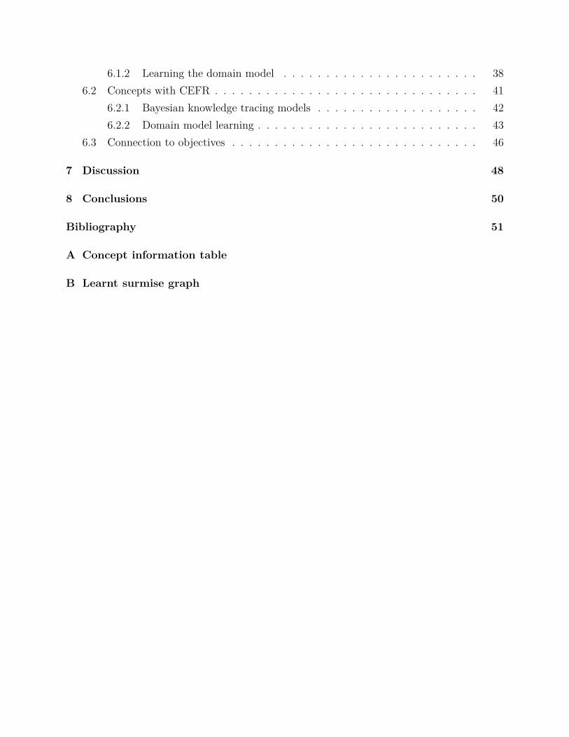
6.1.2 Learning the domain model . . . . . . . . . . . . . . . . . . . . . . . 386.2 Concepts with CEFR . . . . . . . . . . . . . . . . . . . . . . . . . . . . . . . 41

6.2.1 Bayesian knowledge tracing models . . . . . . . . . . . . . . . . . . . 426.2.2 Domain model learning . . . . . . . . . . . . . . . . . . . . . . . . . . 43

6.3 Connection to objectives . . . . . . . . . . . . . . . . . . . . . . . . . . . . . 46

7 Discussion 48

8 Conclusions 50

Bibliography 51

A Concept information table

B Learnt surmise graph

1 Introduction

1.1 Motivation

The quality education has cultivated dramatic awareness with a view to optimizing educationand heading to a sustainable development in the future. The importance of quality educationhas been acknowledged by several researchers forcing them to seek for multiple efficient ways.In the last few years, there has experimented a global evolving trend over different studydomains of utilizing Artificial intelligence or Machine learning in gauging and optimizing thestudying process.

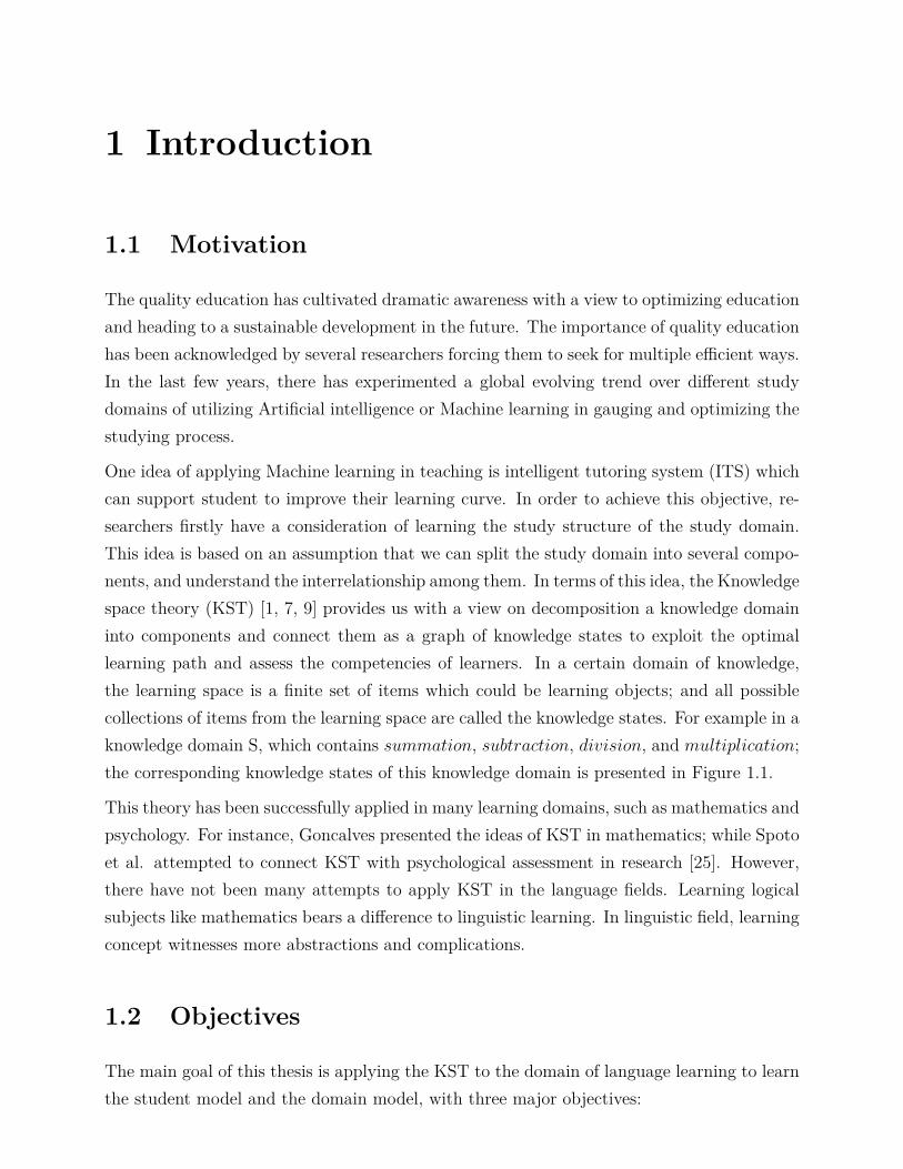
One idea of applying Machine learning in teaching is intelligent tutoring system (ITS) whichcan support student to improve their learning curve. In order to achieve this objective, re-searchers firstly have a consideration of learning the study structure of the study domain.This idea is based on an assumption that we can split the study domain into several compo-nents, and understand the interrelationship among them. In terms of this idea, the Knowledgespace theory (KST) [1, 7, 9] provides us with a view on decomposition a knowledge domaininto components and connect them as a graph of knowledge states to exploit the optimallearning path and assess the competencies of learners. In a certain domain of knowledge,the learning space is a finite set of items which could be learning objects; and all possiblecollections of items from the learning space are called the knowledge states. For example in aknowledge domain S, which contains summation, subtraction, division, and multiplication;the corresponding knowledge states of this knowledge domain is presented in Figure 1.1.

This theory has been successfully applied in many learning domains, such as mathematics andpsychology. For instance, Goncalves presented the ideas of KST in mathematics; while Spotoet al. attempted to connect KST with psychological assessment in research [25]. However,there have not been many attempts to apply KST in the language fields. Learning logicalsubjects like mathematics bears a difference to linguistic learning. In linguistic field, learningconcept witnesses more abstractions and complications.

1.2 Objectives

The main goal of this thesis is applying the KST to the domain of language learning to learnthe student model and the domain model, with three major objectives:

2

Figure 1.1: Example of knowledge states of knowledge domain S

3

1. Tracking the advancement of students: the student model takes the sequence of per-formance of a student A on a concept/skill B to estimate the proficiency level of A onB, and to predict the performance of A on B in the future.

2. Measuring the difficulty of concepts: the student model uses the performance of all stu-dents to learn the correlation between mastery states, mean scores, and score variances,which gives an estimate of the difficulty of the concepts.

3. Proposing a learning plan for students: the domain model learns the “surmise” relation—the prerequisite relation—between concepts in the domain of language learning, toestimate the most suitable learning plan for students based on the history of theirperformance.

To learn the student models to estimate student’s proficiency state, we use two algorithms:BKT and Threshold-based (Section 3.1). The learnt model is able to estimate the proficiencystate (mastery state) of students on concepts based on their performance. The state of onestudent on one concept is labeled “learnt” or “not learnt”. Estimating the state meansestimating whether a student has mastered one concept. The student model can also learnthe mean score and variance of score of each concept, which mean the student model canhelp us measure the hardness of concepts.

To learn the domain model, we construct a surmise graph of the domain as a Bayesiannetwork with each node manifesting for one corresponding concept. Bayesian network is aprobabilistic graphical model, which encodes the conditional dependencies among a set ofvariables in a directed acyclic graph. In the domain of learning Russian, the items are calledconcepts such as “Negative construction”, “I conjugation”, “Negative sentences”, . . . . Weapply five different algorithms (Section 5) to learn the structure of surmise graph from data.The surmise graph encodes the surmise relationship among concepts in topological order.The graph is able to suggest the optimal learning curve for students based on their currentproficiency state and their target of study.

The domain model is able to suggest the optimal learning curve given the proficiency states ofstudents of all concepts. The student is able to estimate the proficiency states of students ofall concepts as the input of the domain model. By the domain model and student model, wecan build a tutoring systems, which has the abilities to track the advancement of students,predict future performance of students, measure the hardness of concepts (feature of thestudent model), and provide the optimal learning curve for students (feature of the domainmodel).

4

1.3 Structure of the thesis

This thesis is organized as follows. Section 2 is the outlines of the data. In Section 3, thebackground review for all solutions and ideas used in this thesis are denoted. Section 4presents related works with this paper. It is followed by a description of our solutions inSection 5. The empirical experiments of all solutions and methodologies are then presentedin Section 6. Section 7 is the place for discussion of current obstacles and future ideas forthis topic. The last part of this thesis, Section 8, contains the conclusion along with thesummary of the whole paper and the acknowledgement. The final concept graph along withthe concept list and their information can be found on appendix pages.

2 Data

2.1 Data Description

All data for this thesis are collected from the Revita system which is a language learningplatform developed by the cooperation between Computer Science department, Modern Lan-guages department of University of Helsinki and Foreign Languages and Literatures depart-ment of University of Milan [12, 13]. Revita is a part of ICALL, Intelligent Computer-AidedLanguage Learning created to support language education over many universities and orga-nizations in the world.

There are about 5000 questions distributed over 88 concepts and 6 levels of the CommonEuropean Framework of Reference for Languages (CEFR) system which are A1, A2, B1, B2,C1, and C2. Those concepts along with their CEFR information are provided by linguisticexperts in Russian, for instance, teachers from Russian departments. The samples of studentperformances are collected directly from real Russian learners on Revita system. There areabout 500 students having done one or many tests and approximately 4000 test sessions intotal. In each test session, the time is limited and all concepts are asked with a randomizednumber of questions sampled from the corresponding question bank; however, it is unneces-sary that students answer all given questions in a test session. There are approximately 300questions in each test in such way that each question belongs to only one concept and allconcept is presented in each test session with at least one question. The timestamps, studentidentity numbers, and question CEFR levels are also recorded along with all questions ineach test session.

2.2 Data Pre-processing

This thesis presents two experiments, the first using the original 88 concepts without takinginto account their CEFR levels, and the second using a combination of concepts with CEFRlevels. For example, concept “6, Lexicology. Lexical semantics” is distributed over threeCEFR levels: B1, B2, and C1. In the second experiment, this concept is considered as 3different concepts “6B1”, “6B2” and “6C1”. The total number of these “refined” conceptsproduced by this combination process is 127. Thus we have two experiments:

1. with the set of original 88 concepts, named concepts without CEFR, and

6

2. with the set of 127 fragmented concepts, named concepts with CEFR.

The methodology of our solution contains three main steps. Firstly, we attempt to learnthe models tracking student’s advancement. In the second step, we use the models trainedafter the first step to estimate the corresponding advancement states. Lastly, we recoverthe interrelationship between concepts based on the estimated advancement data from thesecond step. To do so, the accumulated examples are split into three disjoint datasets bygrouping the students. The three disjoint datasets are:

• the “student” set (188 students, 1265 test sessions) used for training the student model,

• the “domain” set (189 students, 1489 test sessions) for constructing the domain model,and

• the “evaluation” set (189 students, 1255 test sessions) for evaluating.

Data of the first student group are used for step 1 in which the student models are built. Thestudent models learnt from the first group are utilized to estimate state data of the secondstudent group. Then, the state data of the second group is used to learn the concept graph(the knowledge structure). The third group is the evaluation data-set for the concept graph.

2.3 Data Table Format

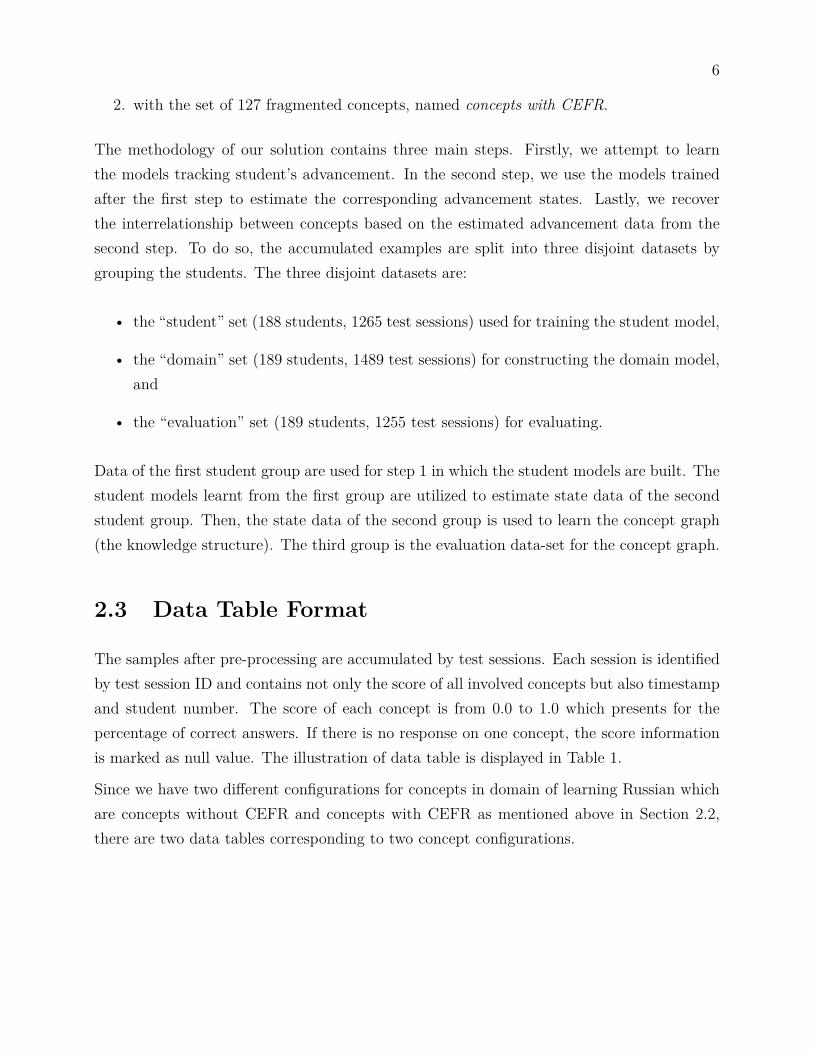
The samples after pre-processing are accumulated by test sessions. Each session is identifiedby test session ID and contains not only the score of all involved concepts but also timestampand student number. The score of each concept is from 0.0 to 1.0 which presents for thepercentage of correct answers. If there is no response on one concept, the score informationis marked as null value. The illustration of data table is displayed in Table 1.

Since we have two different configurations for concepts in domain of learning Russian whichare concepts without CEFR and concepts with CEFR as mentioned above in Section 2.2,there are two data tables corresponding to two concept configurations.

7

Test session Student ID Timestamp Concept 1 Concept 2 ... Concept N001 01 1586203202 0.2 0.6 ... null002 01 1586203206 0.6 null ... 0.9... ... ... ... ... ... ...

999 99 1586203200 1.0 0.8 ... 0.7

Table 2.1: Example of data format

3 Background

3.1 Knowledge space theory

Knowledge space theory (KST) is a framework for identifying the learning structure of aknowledge domain. This theory was invented by Doignon & Falmagne in 1985 [9] and thenimproved by Albert & Lukas in 1999 [1]. The theory assumes that in a certain study field,there is a finite set Q of problem types, skills or concepts representing some learning objectsor levels in that knowledge domain; and set K which contains some subsets of Q. Forillustration, a student needs to master basic knowledge of number in order to understandsome mathematical formulas and be able to handle all basic operations such as addition,subtraction, multiplication and division in a simple equation. Therefore, the study domainof solving a simple equation could be decomposed into two concepts: numbers and operations.However, there are some subsets of Q are not knowledge states (not belong to K) since thesesubsets are not likely to exist. For example, one student cannot understand gradient withoutany knowledge about number and operations, hence there is likely no knowledge state containsgradient without numbers and operations.

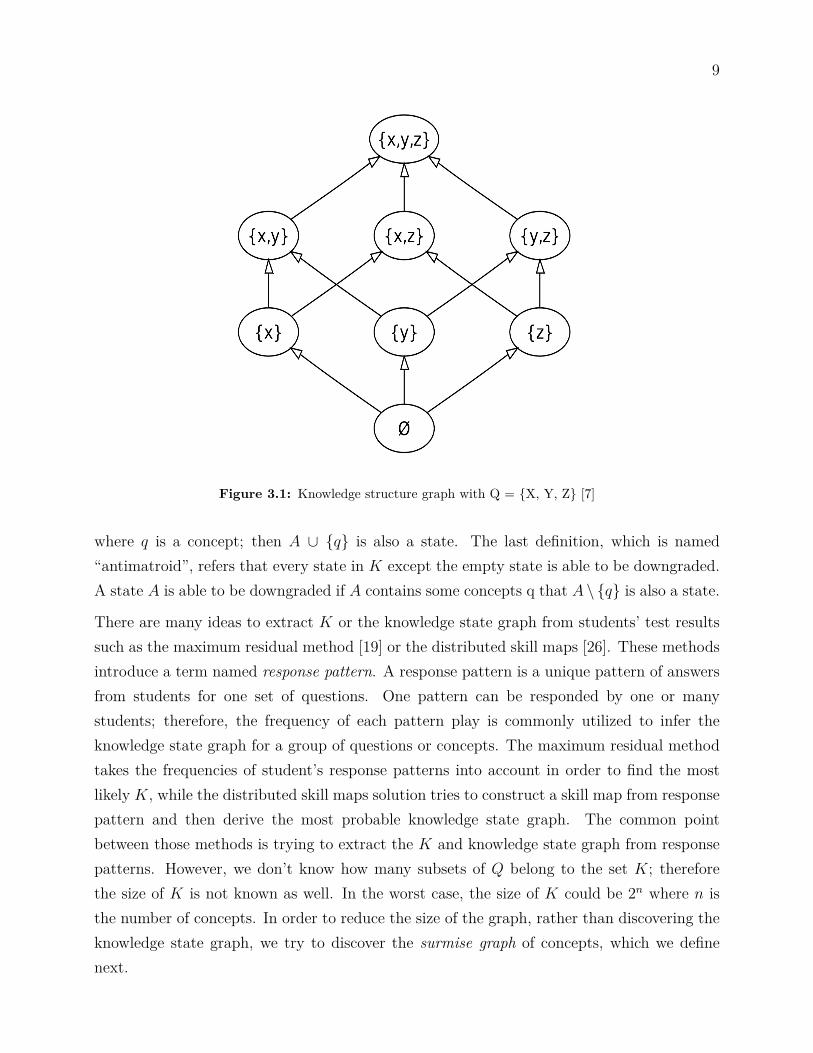
The collection K of subsets of Q which includes the empty set and the Q itself is considered asthe set of knowledge states of the study domain. All elements of K are related to each otherin a topological order and together they construct a Bayesian network (Section 3.2) that theroot node stands for the empty knowledge state and the last node stands for a knowledgestate which contains all skills in Q. This Bayesian network is named the knowledge stategraph describing the study domain. For illustration, Figure 3.1 presents an example graphof a knowledge structure with Q = {X, Y, Z}. In KST, set K and set Q define the domainmodel of a study field which is the first objective of an ITS.

To discover Q and K, there are some definitions that have been denoted by Doignon andFalmagne in paper “Knowledge space and learning space” [8]. Firstly, the discriminativedefinition that for all concepts X and Y , the two collections of all knowledge states containingX or Y are identical if and only if X is equal Y . The second definition relates to learningsmoothness that if a knowledge state A contains knowledge state B then there is at leastone topological path to reach A from B by learning concept one by one. The third definitionstates learning consistency which implies that understanding more concepts does not limitlearning new things. For example, if there is a state A contains state B and state B ∪ {q}

9

Figure 3.1: Knowledge structure graph with Q = {X, Y, Z} [7]

where q is a concept; then A ∪ {q} is also a state. The last definition, which is named“antimatroid”, refers that every state in K except the empty state is able to be downgraded.A state A is able to be downgraded if A contains some concepts q that A \ {q} is also a state.

There are many ideas to extract K or the knowledge state graph from students’ test resultssuch as the maximum residual method [19] or the distributed skill maps [26]. These methodsintroduce a term named response pattern. A response pattern is a unique pattern of answersfrom students for one set of questions. One pattern can be responded by one or manystudents; therefore, the frequency of each pattern play is commonly utilized to infer theknowledge state graph for a group of questions or concepts. The maximum residual methodtakes the frequencies of student’s response patterns into account in order to find the mostlikely K, while the distributed skill maps solution tries to construct a skill map from responsepattern and then derive the most probable knowledge state graph. The common pointbetween those methods is trying to extract the K and knowledge state graph from responsepatterns. However, we don’t know how many subsets of Q belong to the set K; thereforethe size of K is not known as well. In the worst case, the size of K could be 2n where n isthe number of concepts. In order to reduce the size of the graph, rather than discovering theknowledge state graph, we try to discover the surmise graph of concepts, which we definenext.

10

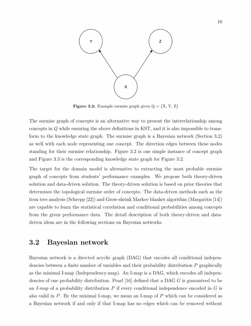
Figure 3.2: Example surmise graph given Q = {X, Y, Z}

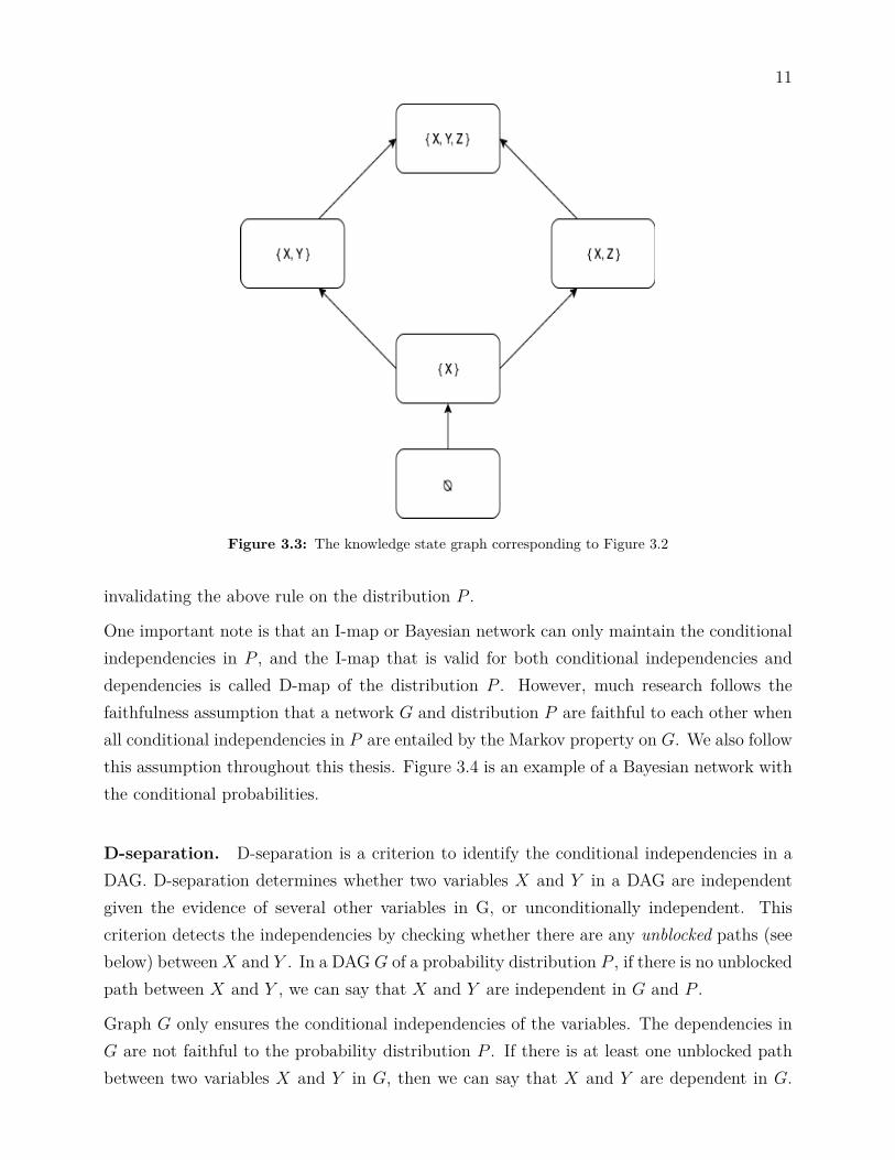
The surmise graph of concepts is an alternative way to present the interrelationship amongconcepts in Q while ensuring the above definitions in KST, and it is also impossible to trans-form to the knowledge state graph. The surmise graph is a Bayesian network (Section 3.2)as well with each node representing one concept. The direction edges between these nodesstanding for their surmise relationship. Figure 3.2 is one simple instance of concept graphand Figure 3.3 is the corresponding knowledge state graph for Figure 3.2.

The target for the domain model is alternative to extracting the most probable surmisegraph of concepts from students’ performance examples. We propose both theory-drivensolution and data-driven solution. The theory-driven solution is based on prior theories thatdetermines the topological surmise order of concepts. The data-driven methods such as theitem tree analysis (Schrepp [22]) and Grow-shrink Markov blanket algorithm (Margaritis [14])are capable to learn the statistical correlation and conditional probabilities among conceptsfrom the given performance data. The detail description of both theory-driven and data-driven ideas are in the following sections on Bayesian networks.

3.2 Bayesian network

Bayesian network is a directed acyclic graph (DAG) that encodes all conditional indepen-dencies between a finite number of variables and their probability distribution P graphicallyas the minimal I-map (Independency-map). An I-map is a DAG, which encodes all indepen-dencies of one probability distribution. Pearl [16] defined that a DAG G is guaranteed to bean I-map of a probability distribution P if every conditional independence encoded in G isalso valid in P . By the minimal I-map, we mean an I-map of P which can be considered asa Bayesian network if and only if that I-map has no edges which can be removed without

11

Figure 3.3: The knowledge state graph corresponding to Figure 3.2

invalidating the above rule on the distribution P .

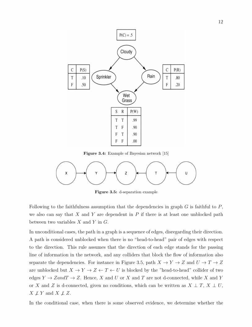
One important note is that an I-map or Bayesian network can only maintain the conditionalindependencies in P , and the I-map that is valid for both conditional independencies anddependencies is called D-map of the distribution P . However, much research follows thefaithfulness assumption that a network G and distribution P are faithful to each other whenall conditional independencies in P are entailed by the Markov property on G. We also followthis assumption throughout this thesis. Figure 3.4 is an example of a Bayesian network withthe conditional probabilities.

D-separation. D-separation is a criterion to identify the conditional independencies in aDAG. D-separation determines whether two variables X and Y in a DAG are independentgiven the evidence of several other variables in G, or unconditionally independent. Thiscriterion detects the independencies by checking whether there are any unblocked paths (seebelow) between X and Y . In a DAG G of a probability distribution P , if there is no unblockedpath between X and Y , we can say that X and Y are independent in G and P .

Graph G only ensures the conditional independencies of the variables. The dependencies inG are not faithful to the probability distribution P . If there is at least one unblocked pathbetween two variables X and Y in G, then we can say that X and Y are dependent in G.

12

Figure 3.4: Example of Bayesian network [15]

Figure 3.5: d-separation example

Following to the faithfulness assumption that the dependencies in graph G is faithful to P ,we also can say that X and Y are dependent in P if there is at least one unblocked pathbetween two variables X and Y in G.

In unconditional cases, the path in a graph is a sequence of edges, disregarding their direction.A path is considered unblocked when there is no “head-to-head” pair of edges with respectto the direction. This rule assumes that the direction of each edge stands for the passingline of information in the network, and any colliders that block the flow of information alsoseparate the dependencies. For instance in Figure 3.5, path X → Y → Z and U → T → Z

are unblocked but X → Y → Z ← T ← U is blocked by the ”head-to-head” collider of twoedges Y → ZandT → Z. Hence, X and U or X and T are not d-connected, while X and Y

or X and Z is d-connected, given no conditions, which can be written as X ⊥ T , X ⊥ U ,X 6⊥ Y and X 6⊥ Z.

In the conditional case, when there is some observed evidence, we determine whether the

13

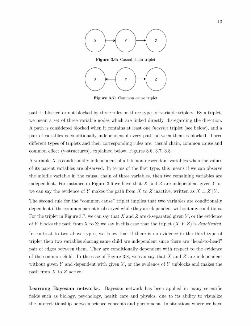
Figure 3.6: Casual chain triplet

Figure 3.7: Common cause triplet

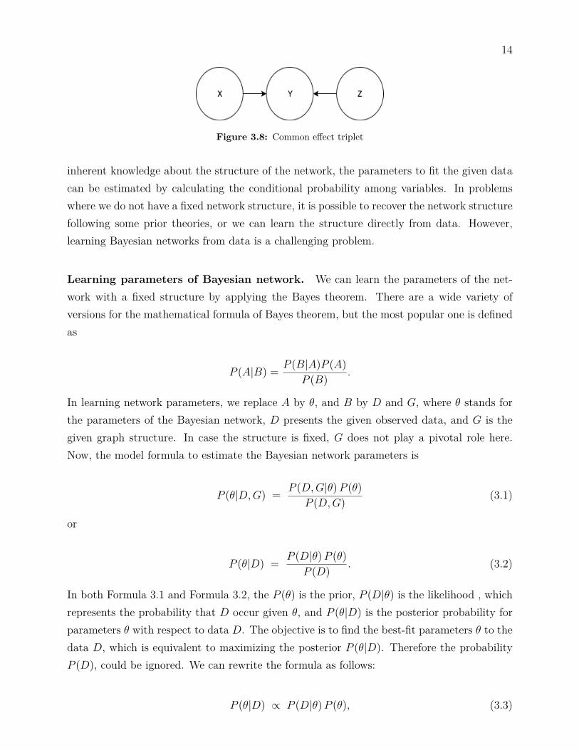
path is blocked or not blocked by three rules on three types of variable triplets. By a triplet,we mean a set of three variable nodes which are linked directly, disregarding the direction.A path is considered blocked when it contains at least one inactive triplet (see below), and apair of variables is conditionally independent if every path between them is blocked. Threedifferent types of triplets and their corresponding rules are: casual chain, common cause andcommon effect (v-structures), explained below, Figures 3.6, 3.7, 3.8.

A variable X is conditionally independent of all its non-descendant variables when the valuesof its parent variables are observed. In terms of the first type, this means if we can observethe middle variable in the causal chain of three variables, then two remaining variables areindependent. For instance in Figure 3.6 we have that X and Z are independent given Y orwe can say the evidence of Y makes the path from X to Z inactive, written as X ⊥ Z |Y .

The second rule for the “common cause” triplet implies that two variables are conditionallydependent if the common parent is observed while they are dependent without any conditions.For the triplet in Figure 3.7, we can say that X and Z are d-separated given Y , or the evidenceof Y blocks the path from X to Z; we say in this case that the triplet (X, Y, Z) is deactivated.

In contrast to two above types, we know that if there is no evidence in the third type oftriplet then two variables sharing same child are independent since there are “head-to-head”pair of edges between them. They are conditionally dependent with respect to the evidenceof the common child. In the case of Figure 3.8, we can say that X and Z are independentwithout given Y and dependent with given Y , or the evidence of Y unblocks and makes thepath from X to Z active.

Learning Bayesian networks. Bayesian network has been applied in many scientificfields such as biology, psychology, health care and physics, due to its ability to visualizethe interrelationship between science concepts and phenomena. In situations where we have

14

Figure 3.8: Common effect triplet

inherent knowledge about the structure of the network, the parameters to fit the given datacan be estimated by calculating the conditional probability among variables. In problemswhere we do not have a fixed network structure, it is possible to recover the network structurefollowing some prior theories, or we can learn the structure directly from data. However,learning Bayesian networks from data is a challenging problem.

Learning parameters of Bayesian network. We can learn the parameters of the net-work with a fixed structure by applying the Bayes theorem. There are a wide variety ofversions for the mathematical formula of Bayes theorem, but the most popular one is definedas

P (A|B) = P (B|A)P (A)P (B) .

In learning network parameters, we replace A by θ, and B by D and G, where θ stands forthe parameters of the Bayesian network, D presents the given observed data, and G is thegiven graph structure. In case the structure is fixed, G does not play a pivotal role here.Now, the model formula to estimate the Bayesian network parameters is

P (θ|D,G) = P (D,G|θ)P (θ)P (D,G) (3.1)

or

P (θ|D) = P (D|θ)P (θ)P (D) . (3.2)

In both Formula 3.1 and Formula 3.2, the P (θ) is the prior, P (D|θ) is the likelihood , whichrepresents the probability that D occur given θ, and P (θ|D) is the posterior probability forparameters θ with respect to data D. The objective is to find the best-fit parameters θ to thedata D, which is equivalent to maximizing the posterior P (θ|D). Therefore the probabilityP (D), could be ignored. We can rewrite the formula as follows:

P (θ|D) ∝ P (D|θ)P (θ), (3.3)

15

where ∝ means “proportional to.” To find the parameters of the graph, we find the value ofθ, which derives the maximum value of P (θ|D) or P (D|θ).

The posterior P (θ|D) can be maximized by maximum a posteriori estimation (MAP). MAPis useful to avoid overfitting in the situation when we have limited examples. MaximizingP (θ|D) is equivalent to maximizing P (D|θ)P (θ) according to Formula 3.3. MaximizingP (D|θ) can be solved by Maximum Likelihood Estimation (MLE). MLE is equivalent to MAPif the prior P (θ) is uniform, which means maximizing P (θ|D) is equivalent to maximizingP (D|θ).

Learning the structure of Bayesian network. In the literature, there are two basicdata-driven solutions to extract the structure of the Bayesian network from data. The firstsolution is a score-based method [28]. This method assigns a formula to calculate a scorefor each version of the graph. The formula for the score usually describes the fitting of thegraph to the observations, which is presented in Formula (3.4).

Score(G,D) = P (G|D), (3.4)

where G represents one version of network structure and D is the data. We can apply Bayestheorem here to expand Formula 3.4) to Formula (3.5.

Score(G,D) = P (G|D) = P (D|G)P (G)P (D) . (3.5)

In order to find the greatest score, we need to find structure G that maximizes the P (G|D).The denominator P (D) does not depend on G; therefore, the maximization depends onthe numerator P (D|G)P (G). In the numerator, the probability distribution of G is our priorknowledge on G, and we assume that P (G) is uniform and can be ignored. Hence, maximizingP (D|G) or P (G|D) results in the optimal score.

The second approach is constraint-based method [28], which constructs the network structurebased on the status of conditional independence to learn the relationship among each pair ofvariables. We need to follow the above faithfulness assumption of Bayesian network for thismethod. The core component of this idea is the conditional independence test Ind(Xi;Xj|S)to check the independence between Xi and Xj given the evidence S. According to thefaithfulness assumption, if Ind(Xi;Xj|S) returns that two variables Xi and Xj are dependent(or independent) given the evidence of S, then Xi and Xj are not d-separated (or d-separated,respectively) given the evidence of S. This method can be exemplified by SGS algorithmSpirtes, Glymour & Scheines [24], or Inductive Causation (IC) algorithm [18]. Both the

16

SGS algorithm and IC algorithm initializes with a complete non-directed graph, and keepsremoving edges following the independence check Ind(Xi;Xj|S), for each pair of variables.

The common problem of the two above structure learning methods is their time complexity.Those methods search for the best fit version of structure on data where the possible numberof structures is 2n, where n is the number of variables in the domain. For instance, the SGSalgorithm computes the independencies for each pair of variables X and Y , with respect toall 2n−2 subsets of set Q, containing all variables in the domain except the two variablesX and Y . Those methods with exponential complexity are impractical in our situation,when our domain is comprised of up to 127 variables (Section 2.2). Therefore, we introducetwo alternative methods in the thesis. The first is a version of the score-based method,which is modified to find an approximate answer to save computation time. The second isan independence-based algorithm, called the Grow-shrink Markov blanket algorithm, whichexploits the properties of the Markov blanket in a Bayesian network.

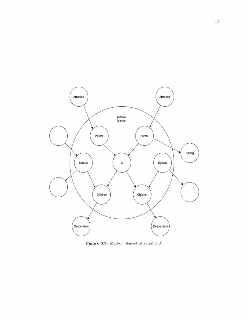
Markov blanket. For Bayesian networks in particular and directed acyclic graph in gen-eral, the Markov blanket of a node X in the graph is defined as the set of its parents, childrenand spouses, where the spouses are the nodes that share the one or more same children withX. More detail on Markov blanket can be found in the paper “Probabilistic Reasoning inIntelligent Systems: Networks of Plausible Inference” published by Pearl in 1988 [17]. Fig-ure 3.9 is an example of Markov blanket for variable X. The evidence of X’s parents blockall paths from all of X’s ancestors (except X’s parents) to X with respect to the first rule ofd-separation, while the second rule of d-separation declares that the evidence of X’s parentsalso blocks all paths from X’s siblings, where the siblings are nodes sharing one or morecommon parents with X. The evidence of X’s children blocks all paths from X to X’s de-scendants (except X’s children) due to the first rule. The evidence of spouses of X makes allpaths from all X’s children to all outside nodes of the Markov blanket inactive. Accordingly,we have that for each variable X in the network if we can observe all variables in its Markovblanket then this variable X is independent of all other variables in the graph. In otherwords, the Markov blanket is all we need to predict the information of that node.

3.3 Grow-shrink Markov blanket algorithm

The Grow-shrink Markov blanket algorithm is described by Margaritis in his doctoral thesis[14]. He indicates that the algorithm focuses on the usage of Markov blanket in reconstructingthe network structure. According to the above definition of Markov blanket, we have that allvariables (except the spouses) in a Markov blanket of a variable X are the direct neighbors

17

Figure 3.9: Markov blanket of variable X

18

of X, and the evidence of the Markov blanket of X d-separates X from all other variables inthe domain. The algorithm exploits the blanket to find all neighbors for each variable, thenestimates the direction for each connection to their neighbors.

Step 1—Markov blanket estimation. First, we need to estimate the Markov blanketfor each variable. There are two main phases to do so, which are “Growing phase” and“Shrinking phase”. Margaritis [14] defines these phases as the following pseudo-code:

Algorithm 1 Pseudo-code to extract Markov blanket1: 1. Initialization:2: S ← ∅3: U ← All variables in domain,4: X ← considering variable

5:6: 2. Growing phase:7: while ∃Y ∈ U − {X} such as X 6⊥ Y |S do8: S ← S ∪ {Y }9: end while

10:

11: 3. Shrinking phase:12: while ∃Y ∈ S such as X ⊥ Y |S − {Y } do13: S ← S − {Y }14: end while15:

16: 4. Return S as Markov blanket of X

According to the above algorithm, the growing step begins with an empty set S and keepsadding into S the variables in the domain, except the considered variable that is dependenton X with respect to current content of S. This phase simple tries to find a subset S of allvariables which does not violate the property of Markov blanket, that a blanket of a variableshould isolate it to other variables. However, this first stage does not guarantee that S isthe Markov blanket of X; therefore the shrinking phase shrinks the redundant variables ofS. The faithfulness assumption declares that any variable Y in blanket of X is dependent onX given the evidence of the blanket without Y , or we can say Y and X is d-connected givenBlanket(X) − {Y },∀Y ∈ Blanket(X). The shrink phase filters out the redundant variablein S that do not satisfy the above faithfulness assumption, then returns the Markov blanketof variable X.

19

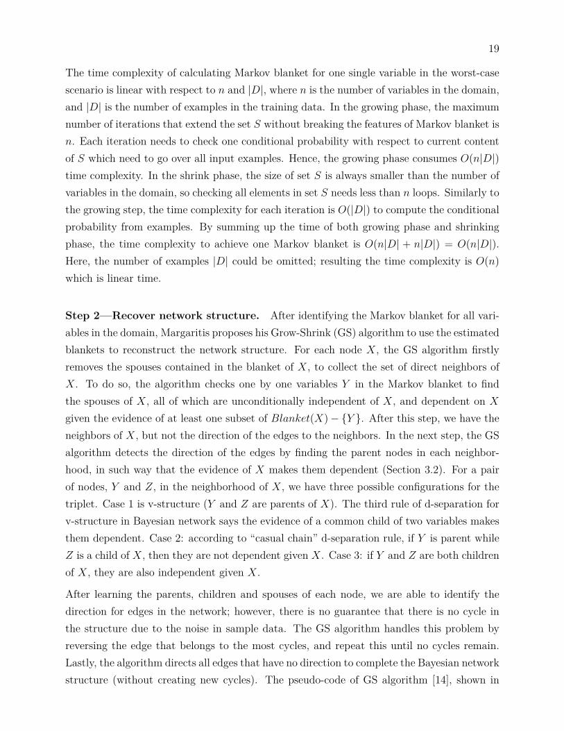
The time complexity of calculating Markov blanket for one single variable in the worst-casescenario is linear with respect to n and |D|, where n is the number of variables in the domain,and |D| is the number of examples in the training data. In the growing phase, the maximumnumber of iterations that extend the set S without breaking the features of Markov blanket isn. Each iteration needs to check one conditional probability with respect to current contentof S which need to go over all input examples. Hence, the growing phase consumes O(n|D|)time complexity. In the shrink phase, the size of set S is always smaller than the number ofvariables in the domain, so checking all elements in set S needs less than n loops. Similarly tothe growing step, the time complexity for each iteration is O(|D|) to compute the conditionalprobability from examples. By summing up the time of both growing phase and shrinkingphase, the time complexity to achieve one Markov blanket is O(n|D| + n|D|) = O(n|D|).Here, the number of examples |D| could be omitted; resulting the time complexity is O(n)which is linear time.

Step 2—Recover network structure. After identifying the Markov blanket for all vari-ables in the domain, Margaritis proposes his Grow-Shrink (GS) algorithm to use the estimatedblankets to reconstruct the network structure. For each node X, the GS algorithm firstlyremoves the spouses contained in the blanket of X, to collect the set of direct neighbors ofX. To do so, the algorithm checks one by one variables Y in the Markov blanket to findthe spouses of X, all of which are unconditionally independent of X, and dependent on X

given the evidence of at least one subset of Blanket(X)− {Y }. After this step, we have theneighbors of X, but not the direction of the edges to the neighbors. In the next step, the GSalgorithm detects the direction of the edges by finding the parent nodes in each neighbor-hood, in such way that the evidence of X makes them dependent (Section 3.2). For a pairof nodes, Y and Z, in the neighborhood of X, we have three possible configurations for thetriplet. Case 1 is v-structure (Y and Z are parents of X). The third rule of d-separation forv-structure in Bayesian network says the evidence of a common child of two variables makesthem dependent. Case 2: according to “casual chain” d-separation rule, if Y is parent whileZ is a child of X, then they are not dependent given X. Case 3: if Y and Z are both childrenof X, they are also independent given X.

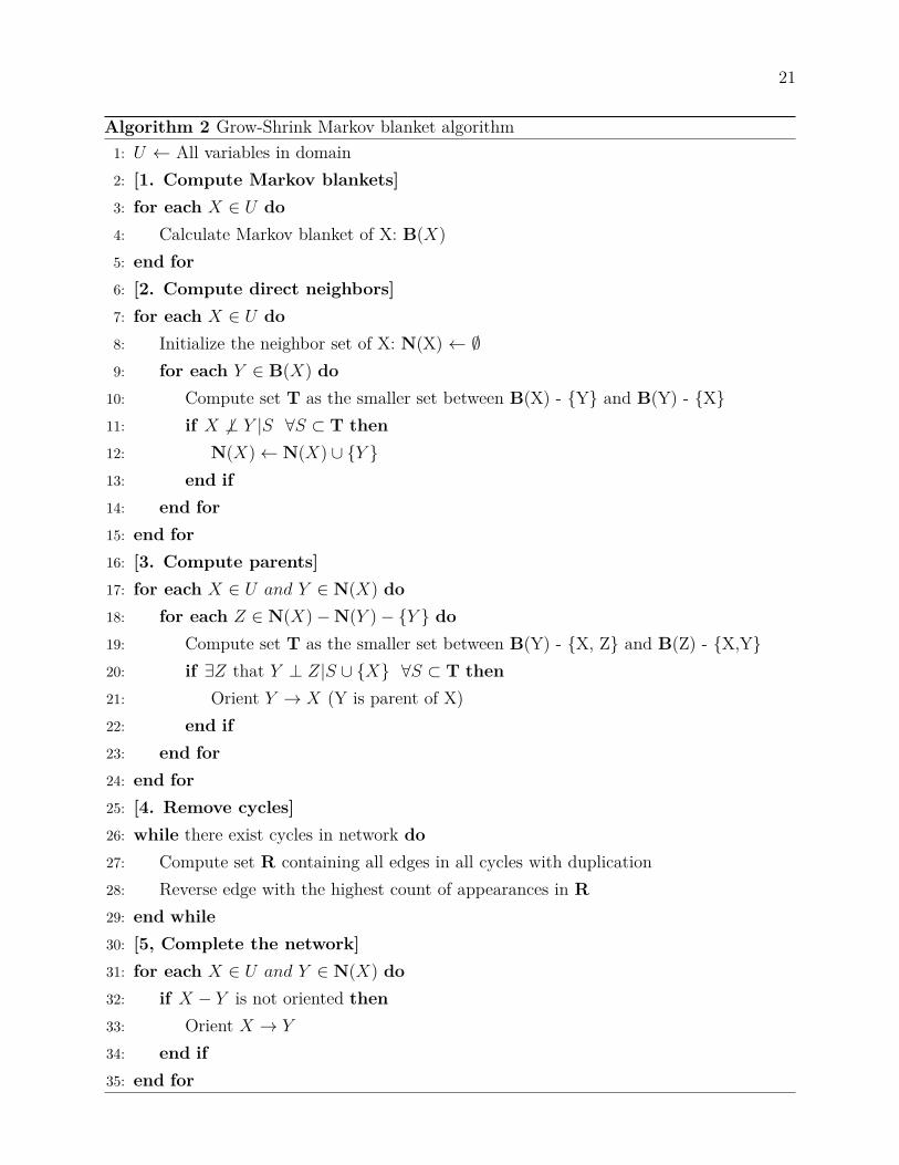
After learning the parents, children and spouses of each node, we are able to identify thedirection for edges in the network; however, there is no guarantee that there is no cycle inthe structure due to the noise in sample data. The GS algorithm handles this problem byreversing the edge that belongs to the most cycles, and repeat this until no cycles remain.Lastly, the algorithm directs all edges that have no direction to complete the Bayesian networkstructure (without creating new cycles). The pseudo-code of GS algorithm [14], shown in

20

Algorithm 2.

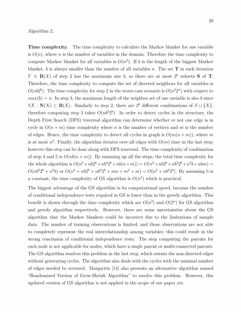
Time complexity. The time complexity to calculate the Markov blanket for one variableis O(n), where n is the number of variables in the domain. Therefore the time complexity tocompute Markov blanket for all variables is O(n2). If b is the length of the biggest Markovblanket, b is always smaller than the number of all variables n. The set T in each iterationY ∈ B(X) of step 2 has the maximum size b, so there are at most 2b subsets S of T.Therefore, the time complexity to compute the set of directed neighbors for all variables isO(nb2b). The time complexity for step 2 in the worst-case scenario is O(n22n) with respect tomax(b) = n. In step 3, the maximum length of the neighbor set of one variable is also b since∀X : N(X) ⊂ B(X). Similarly to step 2, there are 2b different combinations of S ∪ {X},therefore computing step 3 takes O(nb22b). In order to detect cycles in the structure, theDepth First Search (DFS) traversal algorithm can determine whether or not one edge is incycle in O(n + m) time complexity where n is the number of vertices and m is the numberof edges. Hence, the time complexity to detect all cycles in graph is O(m(n+m)), where mis at most n2. Finally, the algorithm iterates over all edges with O(m) time in the last step;however this step can be done along with DFS traversal. The time complexity of combinationof step 4 and 5 is O(nb(n+m)). By summing up all the steps, the total time complexity forthe whole algorithm is O(n2 +nb2b+nb22b+nb(n+m)) = O(n2 +nb2b+nb22b+n2b+nbm) =O(nb22b + n2b) or O(n2 + nb2b + nb22b +mn+m2 +m) = O(n2 + nb22b). By assuming b isa constant, the time complexity of GS algorithm is O(n2) which is practical.

The biggest advantage of the GS algorithm is its computational speed, because the numberof conditional independence tests required in GS is lower than in the greedy algorithm. Thisbenefit is shown through the time complexity which are O(n2) and O(2n) for GS algorithmand greedy algorithm respectively. However, there are some uncertainties about the GSalgorithm that the Markov blankets could be incorrect due to the limitations of sampledata. The number of training observations is limited, and those observations are not ableto completely represent the real interrelationship among variables; this could result in thewrong conclusion of conditional independence tests. The step computing the parents foreach node is not applicable for nodes, which have a single parent or multi-connected parents.The GS algorithm resolves this problem in the last step, which orients the non-directed edgeswithout generating cycles. The algorithm also deals with the cycles with the minimal numberof edges needed be reversed. Margaritis [14] also presents an alternative algorithm named“Randomized Version of Grow-Shrink Algorithm” to resolve this problem. However, thisupdated version of GS algorithm is not applied in the scope of our paper yet.

21

Algorithm 2 Grow-Shrink Markov blanket algorithm1: U ← All variables in domain2: [1. Compute Markov blankets]3: for each X ∈ U do4: Calculate Markov blanket of X: B(X)5: end for6: [2. Compute direct neighbors]7: for each X ∈ U do8: Initialize the neighbor set of X: N(X) ← ∅9: for each Y ∈ B(X) do

10: Compute set T as the smaller set between B(X) - {Y} and B(Y) - {X}11: if X 6⊥ Y |S ∀S ⊂ T then12: N(X)← N(X) ∪ {Y }13: end if14: end for15: end for16: [3. Compute parents]17: for each X ∈ U and Y ∈ N(X) do18: for each Z ∈ N(X)−N(Y )− {Y } do19: Compute set T as the smaller set between B(Y) - {X, Z} and B(Z) - {X,Y}20: if ∃Z that Y ⊥ Z|S ∪ {X} ∀S ⊂ T then21: Orient Y → X (Y is parent of X)22: end if23: end for24: end for25: [4. Remove cycles]26: while there exist cycles in network do27: Compute set R containing all edges in all cycles with duplication28: Reverse edge with the highest count of appearances in R29: end while30: [5, Complete the network]31: for each X ∈ U and Y ∈ N(X) do32: if X − Y is not oriented then33: Orient X → Y

34: end if35: end for

22

Figure 3.10: Example of Hidden Markov model [11]

3.4 Hidden Markov model (HMM)

Hidden Markov model (HMM) and Bayesian network are probabilistic graphical models,which are represented in a DAG. The basic idea of HMM is based on Markov chain. Gagniuc[11] defines that Markov chain is a model encoding the probability of a sequence of variables,where each variable is drawn from some set of variables. This technique is useful to predictthe future of a sequence with respect to the current state. Markov chain is built based on theMarkov assumption, that the probability of one variable in a sequence depends only on theprevious variable. In other words, the present is the only matter, which impacts predictingthe future.

Markov assumption: P (Xi|X1, X2, ..., Xi−1) = P (Xi|Xi−1).

HMM is an extension of the Markov chain which has a sequence of hidden states, which canbe estimated by observing the process of emissions. An HMM is described by N—the numberof possible values of the hidden state (a finite number), and 3 sets of parameters—probabilitydistributions:

1. I - initial state probability distribution,

2. E - emission probability distribution given the state,

3. T - transition probability distribution matrix given the state.

HMM is widely used to find the most probable sequence of hidden states given the sequenceof observations of emissions.

23

3.5 Bayesian knowledge tracing model

Bayesian Knowledge Tracing (BKT) model was presented by Corbett and Anderson in 1994[4], and has been applied widely in ITS field. The fundamental idea behind a BKT model is ahidden Markov model. Our purpose for a student model is to predict students’ mastery stateon one skill through their performance in multiple tests, where the observed results over testsare the emission of their state. In our BKT models, the hidden variables are the masterystates, representing whether student has “learnt” or “not-learnt” a specific skill, while theemission variables are the performance over time of student on that skill. By assessing thestudents’ performance over time, the BKT models can monitor whether the student hasunderstood the skill at each test session. The models also can predict the students’ results ofthat skill for the next upcoming test sessions, based on the latest performance of the student.

Van de Sande [20] has summarized the properties of the BKT models that a BKT modelconsider the hidden states (mastery states) to have only 2 values, which are “learnt” or “notlearnt”, with 4 parameters to optimize:

• P (L0) the probability that student has learnt the skill before the first attempt (corre-sponding to distribution I in HMM)

• P (G) is the probability that a student has not learnt the skill, but luckily guesses thecorrect answer (corresponding to distribution E in HMM)

• P (S) is the probability that a student has learnt the skill, but accidentally makes a slipand gives a wrong answer (corresponding to distribution E in HMM)

• P (T ) is the learning probability that present the chance a student can learn the skillafter one attempt. This P (T ) is assumed to be constant over time (corresponding todistributions T in HMM)

In this paper, we take into account the chance that a student can forget a skill that he haslearnt with probability P (F ) after one test session. The matrix

1 - P(T) P(T)P(F) 1 - P(F)

is the matrix of hidden state transitions. The state transition could be

• learning the skill (from “not-learnt” state to “learnt” state),

• forgetting learnt skill (from “learnt” state to “not-learnt” state)

24

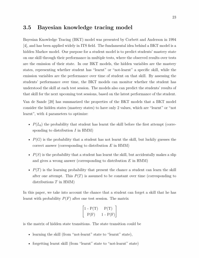
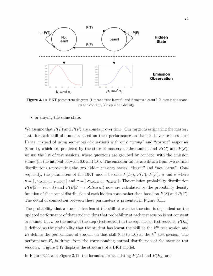
Figure 3.11: BKT parameters diagram (1 means “not learnt”, and 2 means “learnt”. X-axis is the scoreon the concept, Y-axis is the density.

• or staying the same state.

We assume that P (T ) and P (F ) are constant over time. Our target is estimating the masterystate for each skill of students based on their performance on that skill over test sessions.Hence, instead of using sequences of questions with only “wrong” and “correct” responses(0 or 1), which are predicted by the state of mastery of the student and P (G) and P (S);we use the list of test sessions, where questions are grouped by concept, with the emissionvalues (in the interval between 0.0 and 1.0). The emission values are drawn from two normaldistributions representing the two hidden mastery states: “learnt” and “not learnt”. Con-sequently, the parameters of the BKT model become P (L0), P (T ), P (F ), µ and σ whereµ = [ µnot learnt, µlearnt ] and σ = [ σnot learnt, σlearnt ]. The emission probability distributionP (E|S = learnt) and P (E|S = not learnt) now are calculated by the probability densityfunction of the normal distribution of each hidden state rather than based on P (S) and P (G).The detail of connection between these parameters is presented in Figure 3.11.

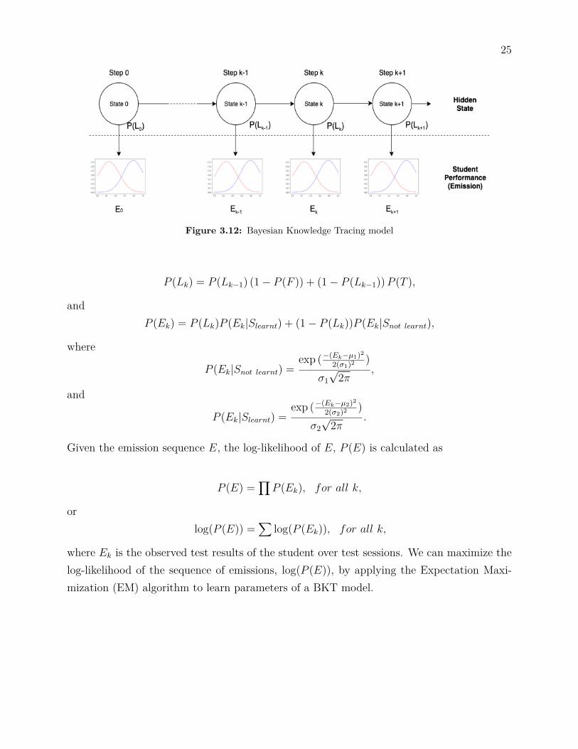
The probability that a student has learnt the skill at each test session is dependent on theupdated performance of that student; thus that probability at each test session is not constantover time. Let k be the index of the step (test session) in the sequence of test sessions; P (Lk)is defined as the probability that the student has learnt the skill at the kth test session andEk defines the performance of student on that skill (0.0 to 1.0) at the kth test session. Theperformance Ek is drawn from the corresponding normal distribution of the state at testsession k. Figure 3.12 displays the structure of a BKT model.

In Figure 3.11 and Figure 3.12, the formulas for calculating P (Lk) and P (Ek) are

25

Figure 3.12: Bayesian Knowledge Tracing model

P (Lk) = P (Lk−1) (1− P (F )) + (1− P (Lk−1))P (T ),

andP (Ek) = P (Lk)P (Ek|Slearnt) + (1− P (Lk))P (Ek|Snot learnt),

where

P (Ek|Snot learnt) =exp (−(Ek−µ1)2

2(σ1)2 )σ1√

2π,

and

P (Ek|Slearnt) =exp (−(Ek−µ2)2

2(σ2)2 )σ2√

2π.

Given the emission sequence E, the log-likelihood of E, P (E) is calculated as

P (E) =∏P (Ek), for all k,

orlog(P (E)) =

∑log(P (Ek)), for all k,

where Ek is the observed test results of the student over test sessions. We can maximize thelog-likelihood of the sequence of emissions, log(P (E)), by applying the Expectation Maxi-mization (EM) algorithm to learn parameters of a BKT model.

4 Related Work

There are three major objectives of our paper, which can be achieved by learning the studentmodel and the domain model. The student model is used to track the advancement of theproficiency level of students on concepts. The domain model is used to represent the structureof the knowledge domain and the connections among all concepts.

Bayesian Knowledge Tracing model is one common technique to track the advancement ofproficiency levels (knowledge states) of students over test sessions based on the students’performance. The standard BKT contains 2 knowledge states which are “learnt” and “not-learnt”, and probabilities to determine the advancement process [bkt˙related]. Yudelsonet al. [bkt˙related] present a promising result for applying BKT on estimating individualknowledge advancement. Zhanga and Yao [29] introduce an update version of the BKT,which has the name is three learning states BKT (TLS-BKT) with 3 states “not-learnt”,“learning” and “learnt”. They believe that the TLS-BKT has a better performance than theoriginal BKT with 2 states. The common point between BKT and TLS-BKT is that theyboth ignore the probability of forgetting. In this thesis, we utilize the standard BKT with 2states, but we take the forgetting into account to track the knowledge states of students.

There are many solutions have been proposed to learn knowledge structure as a correspondingknowledge state graph such as BLIM [10], distributed learning object [26], or maximumresiduals method [19]. One popular mechanism to construct knowledge state graph is usingthe frequency of response pattern from student’s answers. The BLIM algorithm which isinvented by Falmagne and Doignon in 1988 attempts to select the most probable knowledgestates belong to knowledge structureK. To access the states, the algorithm takes into accountboth conditional probability and frequency of knowledge states and answer response patternsfrom students to find the most likely set of knowledge states that generates the observedresponses. Schrepp [23] proposes a method to determine which response pattern is belongto the knowledge domain. He assumes that a response pattern could be generated from oneknowledge state in domain in order find an optimal frequency threshold L in such way that allresponse patterns arriving more than L times are considered as knowledge states in domain.However due to the probability of lucky guess or careless mistake, the frequency non-state-patterns are possibly higher than some state-patterns. To handle this issue, Robusto andStefanutti [19] proposed a mechanism that appends new factor named expected frequencies ofthe response patterns. This expected frequency are able to be obtained by BLIM algorithm[10]. The common point of all the above methods is around observing the frequencies of

27

response patterns to construct a DAG state graph. Constructing a state graph for a largedomain with many concepts and skills or the graph is actually flatten (the component levelis small) consumes a lot of resources since the number of possible knowledge states in thegraph could be exponential (Section 3.1).

To alter the knowledge state graph in order to represent the study domain, the surmisegraph of concepts is a decent candidate where the skill map is still able to encode the sur-mise relationships among skills in domain as well as be easily converted to knowledge stategraph. Desmarais and Gagnon have introduced quite similar idea in their research on learn-ing knowledge structure as item graph [6]. They attempt to present a knowledge domainin form of a Bayesian network presenting the item to item structure. By the item to itemstructure, they mean a DAG structure that represents all surmise relationships between allindividual items in the domain. To do so, they propose two approaches. The first approachlearns the corresponding Bayesian network on observed data with K2 algorithm [3] and PCalgorithm [24]. The second approach believes that the knowledge items in a study domain arein surmise relations following a partial order in which some skills should be mastered beforethe others. They utilize this topological theory in order to iterate over all pair of items tofind the surmise relation in each pair. They consider that itemA � itemB (the mastery ofB precedes the mastery of A) if the following conditions are satisfied

P (B|A) ≥ pc,

andP (A|B) ≥ pc,

andP (B|A) 6= P (B),

where A and B stands for “mastering” item A and item B while A and B presents for “notmastering” these items. They experiment their theory with pc = 0.5.

Hou et al. [12] try to learn the study domain as a skill map structure with Elo-basedmethodology. Their result skill map is flattened, therefore the size of corresponding statestructure is exponential if we try to recover it. Those works of learning item to item structureor the surmise graph of concepts deduces that it is possible to understand the study domainas a surmise graph in which learning surmise graph is more achievable in some scenarios.

Because our second objective is learning the surmise graph, which is a Bayesian network, fromthe mastery data; algorithms for Bayesian network learning also can be used to construct thedomain model. Yuan and Malone [28] show that there are three main approaches to learn a

28

Bayesian network: score-based learning, constraint-based learning, and hybrid methods. Thescore-based learning is NP-hard, which is only suitable for small dataset. The score-basedlearning evaluates the quality of the network by applying a score formula on all possiblenetwork structures in solution space. The constraint-based learning is able to scale thelarge dataset but vulnerable to the noises. The hybrid learning is the integration betweenthe advantages of two base learning methods: score-based learning and constraint-basedlearning. To reduce the running for score-based learning, Yuan and Malone [28] present adynamic programming approach, which constructs the order tree and then they use a searchalgorithm such A* to find the optimal path to the best network structure. By the ordertree, they mean a state space graph for learning Bayesian network, which has the most-topnode is a network structure with only one random node (a start node) and the most-bottomnodes are the network structure with all involved nodes. In terms of constraint-based andhybrid learning, Margaritis [14] presents two solution: Grow-shrink Markov blanket algorithmand Randomized Version of Grow-Shrink Algorithm, which try to identify the conditionalindependence relations from the data to construct the network structure.

5 Research Methodology

The target of this thesis is applying the KST to the domain of language learning to constructthe corresponding domain model and student model with three main objectives). The studentmodel is also used to estimate the mastery data, which is the input for learning the domainmodel.

To learn the domain model, we apply Greedy algorithm and two Bayesian network learn-ing libraries, which are Gobnilp (Globally Optimal Bayesian Network learning using IntegerLinear Programming) [5] and pomegranate [21] as baseline algorithms. We also apply GSalgorithm and Theory-based algorithm to compare with three baseline algorithms (Greedyalgorithm, Gobnilp, pomegranate).

To learn the student model, we use hmmlearn library in Python [27] to learn the BKT modelsbecause the basic idea of BKT models is Hidden Markov Models. We use GaussianHMMclass to construct the HMM of our BKT models since we assume that the score of a masterystate (“learnt” or “not-learnt”) is a variable with normal distribution (Gaussian distribution).

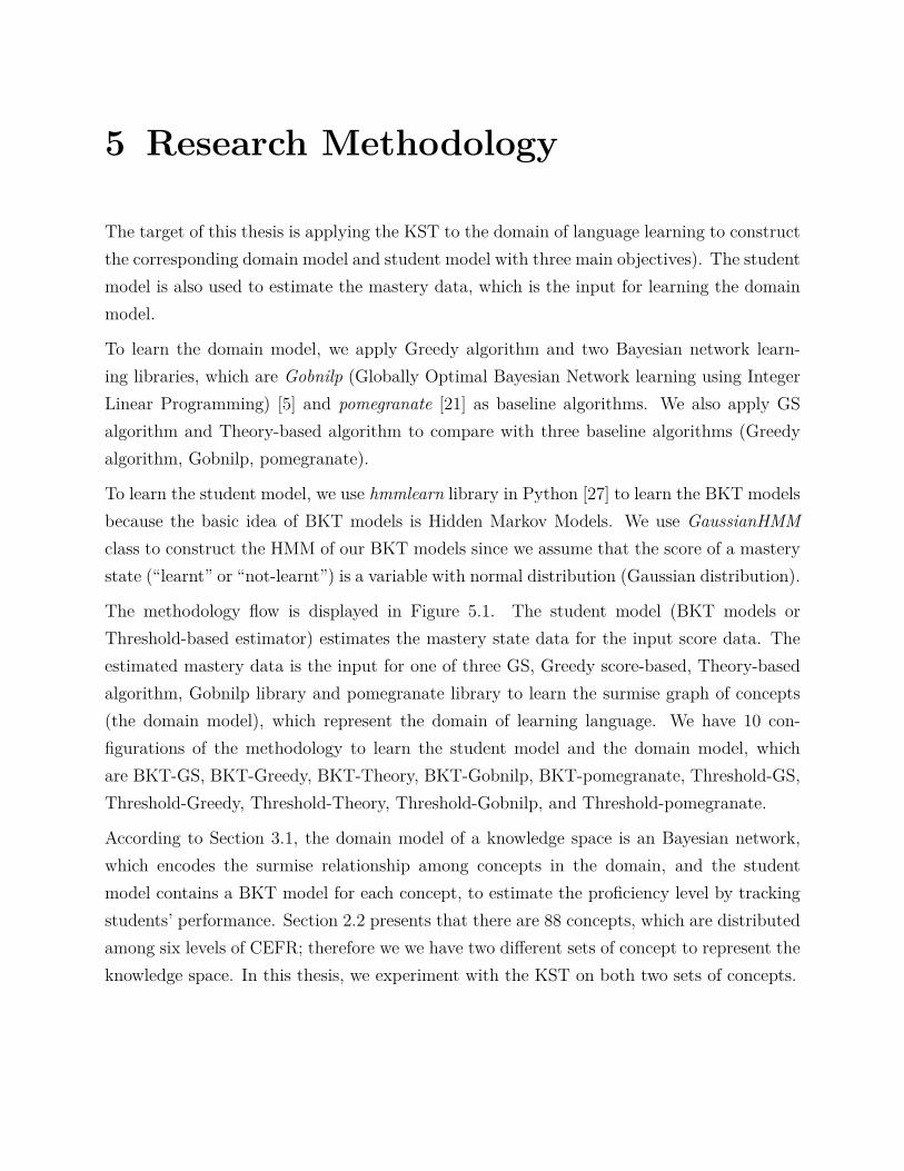
The methodology flow is displayed in Figure 5.1. The student model (BKT models orThreshold-based estimator) estimates the mastery state data for the input score data. Theestimated mastery data is the input for one of three GS, Greedy score-based, Theory-basedalgorithm, Gobnilp library and pomegranate library to learn the surmise graph of concepts(the domain model), which represent the domain of learning language. We have 10 con-figurations of the methodology to learn the student model and the domain model, whichare BKT-GS, BKT-Greedy, BKT-Theory, BKT-Gobnilp, BKT-pomegranate, Threshold-GS,Threshold-Greedy, Threshold-Theory, Threshold-Gobnilp, and Threshold-pomegranate.

According to Section 3.1, the domain model of a knowledge space is an Bayesian network,which encodes the surmise relationship among concepts in the domain, and the studentmodel contains a BKT model for each concept, to estimate the proficiency level by trackingstudents’ performance. Section 2.2 presents that there are 88 concepts, which are distributedamong six levels of CEFR; therefore we we have two different sets of concept to represent theknowledge space. In this thesis, we experiment with the KST on both two sets of concepts.

30

Figure 5.1: Methodology flow

5.1 Learning student models

The function of the student model is analysing the test result of students and assessingtheir mastery state on each skill in each test. We propose two mechanisms to learn thestudent model that can estimate the proficiency levels of students based on their sequence ofperformance. Both techniques are applied the “student” data set.

5.1.1 Threshold-based model

The first is a naive approach, which determines the mastery state by a mastery threshold, θ,(a hyper-parameter, which we tune) on the performance of students for each skill. We saythat a student has learnt the concept (mastery state) if their score on this concept is equalor higher than the mastery threshold. For example, if the score of student A on concept Bin test session C is 0.8 (or 0.6), and the mastery threshold θ is 0.7, then we consider thatstudent A has learnt (or not learnt) concept B, respectively, at the time of session C. Moredetailed examples are displayed in Table 5.1 and Table 5.2.

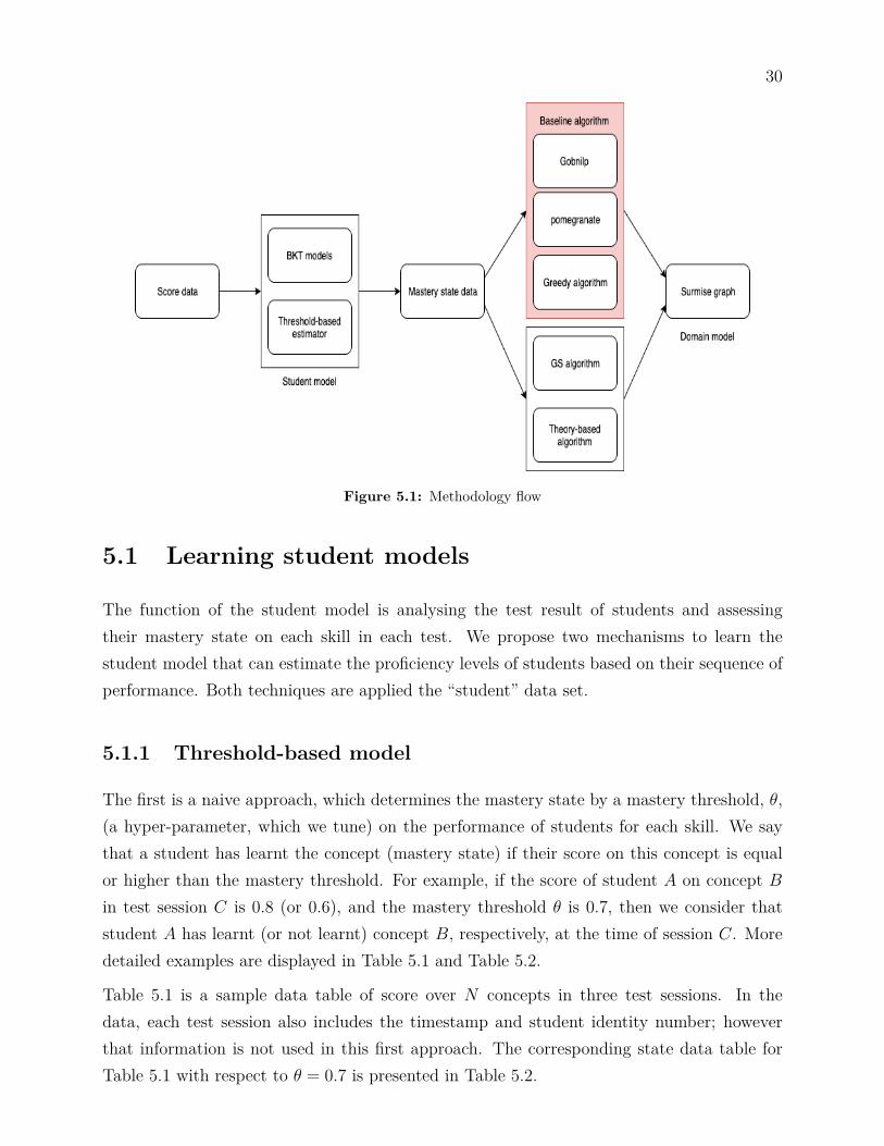
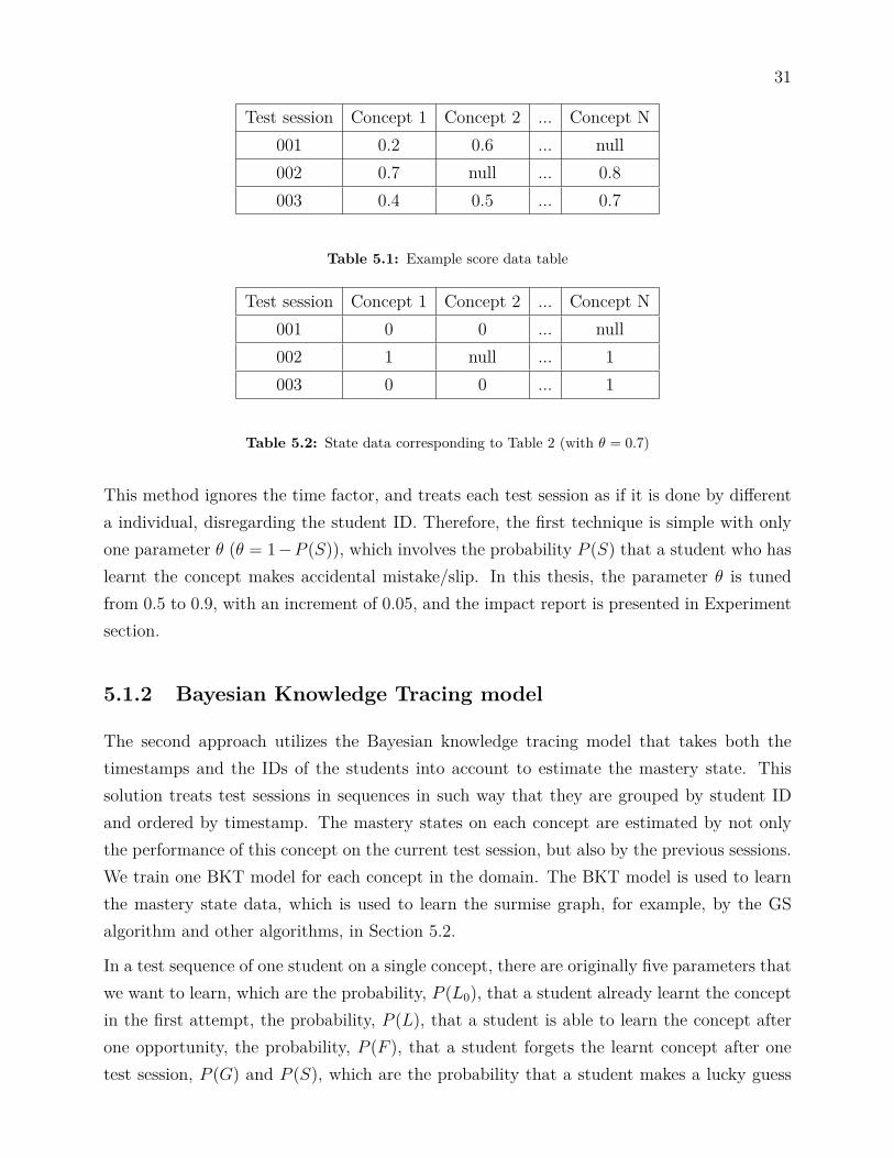
Table 5.1 is a sample data table of score over N concepts in three test sessions. In thedata, each test session also includes the timestamp and student identity number; howeverthat information is not used in this first approach. The corresponding state data table forTable 5.1 with respect to θ = 0.7 is presented in Table 5.2.

31

Test session Concept 1 Concept 2 ... Concept N001 0.2 0.6 ... null002 0.7 null ... 0.8003 0.4 0.5 ... 0.7

Table 5.1: Example score data table

Test session Concept 1 Concept 2 ... Concept N001 0 0 ... null002 1 null ... 1003 0 0 ... 1

Table 5.2: State data corresponding to Table 2 (with θ = 0.7)

This method ignores the time factor, and treats each test session as if it is done by differenta individual, disregarding the student ID. Therefore, the first technique is simple with onlyone parameter θ (θ = 1−P (S)), which involves the probability P (S) that a student who haslearnt the concept makes accidental mistake/slip. In this thesis, the parameter θ is tunedfrom 0.5 to 0.9, with an increment of 0.05, and the impact report is presented in Experimentsection.

5.1.2 Bayesian Knowledge Tracing model

The second approach utilizes the Bayesian knowledge tracing model that takes both thetimestamps and the IDs of the students into account to estimate the mastery state. Thissolution treats test sessions in sequences in such way that they are grouped by student IDand ordered by timestamp. The mastery states on each concept are estimated by not onlythe performance of this concept on the current test session, but also by the previous sessions.We train one BKT model for each concept in the domain. The BKT model is used to learnthe mastery state data, which is used to learn the surmise graph, for example, by the GSalgorithm and other algorithms, in Section 5.2.

In a test sequence of one student on a single concept, there are originally five parameters thatwe want to learn, which are the probability, P (L0), that a student already learnt the conceptin the first attempt, the probability, P (L), that a student is able to learn the concept afterone opportunity, the probability, P (F ), that a student forgets the learnt concept after onetest session, P (G) and P (S), which are the probability that a student makes a lucky guess

32

or a slip. In these parameters, P (G) and P (S) contributes to the score distribution withrespect to the mastery state of the current performance. We use two normal distributions toreplace P (G) and P (S), as we discussed in Section 3.5.

The student models learnt by this step are used to predict the mastery state for the “Domain”dataset as the input for training domain model, as well as to estimate the mastery state datafor the “Evaluation” dataset in order to evaluate the domain model (Section 2.2).

5.2 Learning domain models

The objectives of domain model is to encode the inter-dependencies among concepts in thedomain. Section 3.1 mentions that the domain model is originally a directed acyclic graph ofknowledge states (knowledge state graph), but it can be represented by a surmise graph ofconcepts. As mentioned in Section 2.2, we utilize the student models, which are learnt fromthe student dataset to estimate the mastery state data for the domain dataset. The estimatedstate data of the domain dataset is the input for learning the surmise graph of concepts. Tolearn the surmise graph of concepts from mastery state data, we apply five solutions: GSalgorithm, Theory-based algorithm, Greedy algorithm, Gobnilp library and pomegranatelibrary. The Greedy algorithm, the Gobnilp library and the pomegranate library are baselinemethods, which are used as options for comparison to the GS algorithm and Theory-basedalgorithm. The Gobnilp library [5] and the pomegranate library [21] are Python libraries tolearnt Bayesian network from data. The methodology of experiment with the GS algorithm,the Theory-based algorithm and the Greedy algorithm is described as follows.

5.2.1 Theory-driven method

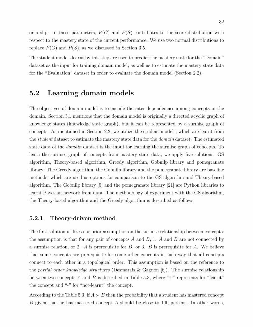
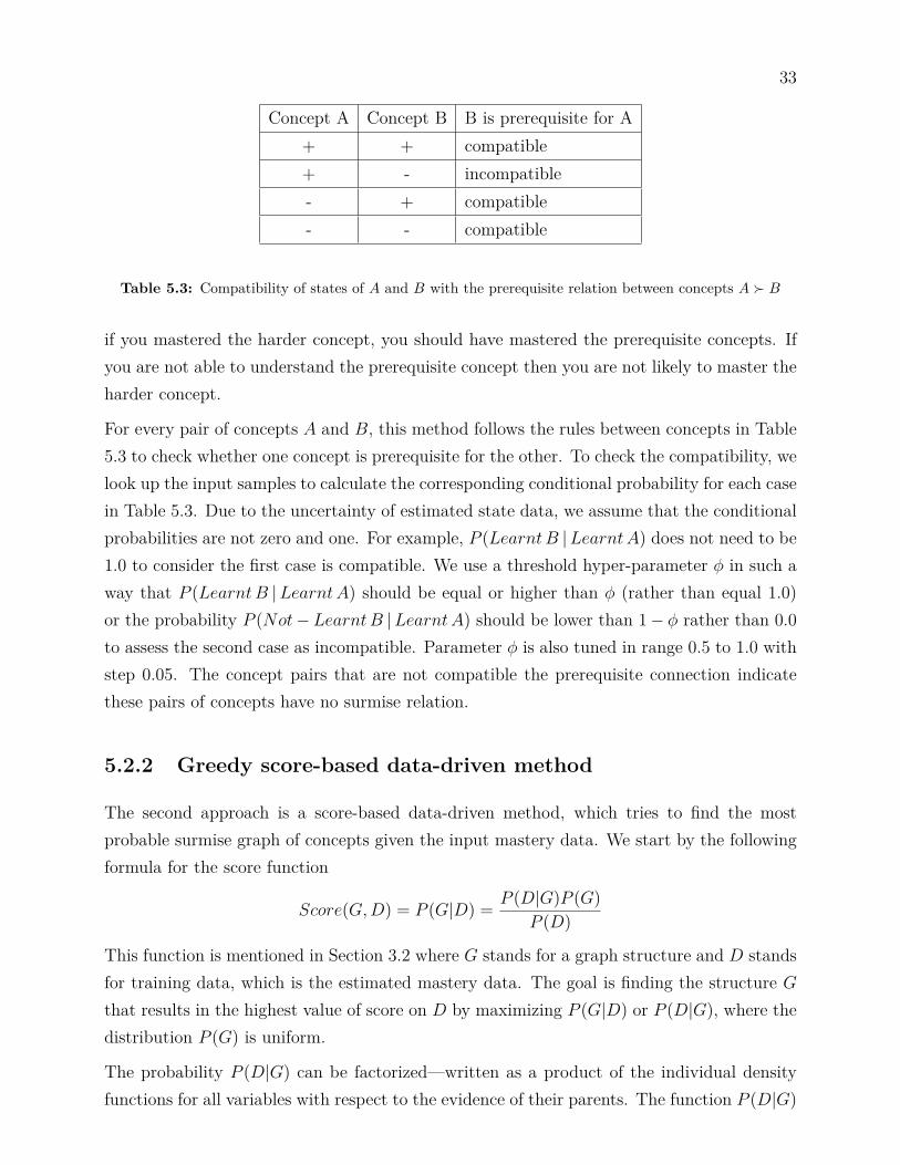
The first solution utilizes our prior assumption on the surmise relationship between concepts:the assumption is that for any pair of concepts A and B, 1. A and B are not connected bya surmise relation, or 2. A is prerequisite for B, or 3. B is prerequisite for A. We believethat some concepts are prerequisite for some other concepts in such way that all conceptsconnect to each other in a topological order. This assumption is based on the reference tothe parital order knowledge structures (Desmarais & Gagnon [6]). The surmise relationshipbetween two concepts A and B is described in Table 5.3, where “+” represents for “learnt”the concept and “-” for “not-learnt” the concept.

According to the Table 5.3, if A � B then the probability that a student has mastered conceptB given that he has mastered concept A should be close to 100 percent. In other words,

33

Concept A Concept B B is prerequisite for A+ + compatible+ - incompatible- + compatible- - compatible

Table 5.3: Compatibility of states of A and B with the prerequisite relation between concepts A � B

if you mastered the harder concept, you should have mastered the prerequisite concepts. Ifyou are not able to understand the prerequisite concept then you are not likely to master theharder concept.

For every pair of concepts A and B, this method follows the rules between concepts in Table5.3 to check whether one concept is prerequisite for the other. To check the compatibility, welook up the input samples to calculate the corresponding conditional probability for each casein Table 5.3. Due to the uncertainty of estimated state data, we assume that the conditionalprobabilities are not zero and one. For example, P (LearntB |LearntA) does not need to be1.0 to consider the first case is compatible. We use a threshold hyper-parameter φ in such away that P (LearntB |LearntA) should be equal or higher than φ (rather than equal 1.0)or the probability P (Not−LearntB |LearntA) should be lower than 1− φ rather than 0.0to assess the second case as incompatible. Parameter φ is also tuned in range 0.5 to 1.0 withstep 0.05. The concept pairs that are not compatible the prerequisite connection indicatethese pairs of concepts have no surmise relation.

5.2.2 Greedy score-based data-driven method

The second approach is a score-based data-driven method, which tries to find the mostprobable surmise graph of concepts given the input mastery data. We start by the followingformula for the score function

Score(G,D) = P (G|D) = P (D|G)P (G)P (D)

This function is mentioned in Section 3.2 where G stands for a graph structure and D standsfor training data, which is the estimated mastery data. The goal is finding the structure Gthat results in the highest value of score on D by maximizing P (G|D) or P (D|G), where thedistribution P (G) is uniform.

The probability P (D|G) can be factorized—written as a product of the individual densityfunctions for all variables with respect to the evidence of their parents. The function P (D|G)

34

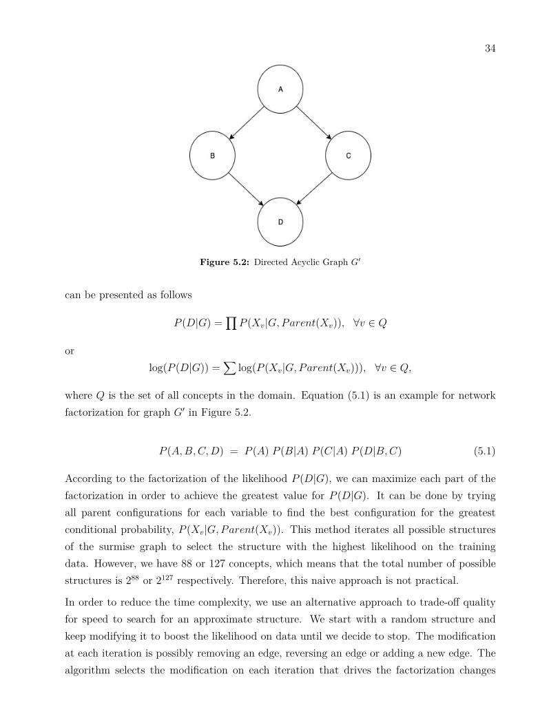
Figure 5.2: Directed Acyclic Graph G′

can be presented as follows

P (D|G) =∏P (Xv|G,Parent(Xv)), ∀v ∈ Q

orlog(P (D|G)) =

∑log(P (Xv|G,Parent(Xv))), ∀v ∈ Q,

where Q is the set of all concepts in the domain. Equation (5.1) is an example for networkfactorization for graph G′ in Figure 5.2.

P (A,B,C,D) = P (A) P (B|A) P (C|A) P (D|B,C) (5.1)

According to the factorization of the likelihood P (D|G), we can maximize each part of thefactorization in order to achieve the greatest value for P (D|G). It can be done by tryingall parent configurations for each variable to find the best configuration for the greatestconditional probability, P (Xv|G,Parent(Xv)). This method iterates all possible structuresof the surmise graph to select the structure with the highest likelihood on the trainingdata. However, we have 88 or 127 concepts, which means that the total number of possiblestructures is 288 or 2127 respectively. Therefore, this naive approach is not practical.

In order to reduce the time complexity, we use an alternative approach to trade-off qualityfor speed to search for an approximate structure. We start with a random structure andkeep modifying it to boost the likelihood on data until we decide to stop. The modificationat each iteration is possibly removing an edge, reversing an edge or adding a new edge. Thealgorithm selects the modification on each iteration that drives the factorization changes

35

with the highest increase of likelihood on the training data. The early stop rules are deter-mined by two factors: the maximum number of iterations (a suitable number of iterationsfor our environment) and a threshold of minimum likelihood score increase after each iter-ation. We experiment with this technique with several initial structures, which includes anempty network (DAG without any edges), a fully-connected network with randomly assigneddirections, and some random networks (not empty and fully-connected).

5.2.3 Grow-shrink Markov blanket data-driven method

Grow-shrink Markov blanket algorithm, as described in Section 3.3, is another data-drivenoption to learn the Bayesian network structure. This algorithm has lower time complexitythan the greedy score-based solution. In this paper, we also attempt to apply the GS algo-rithm [14] to learn the surmise graph of concepts. The detailed explanation of GS algorithmcan be found in Section 3.3. The running time and performance report for GS algorithm ispresented along with two first solutions in Section 6.

6 Experiment Results

The libraries of Gobnilp and pomegranate in Python are not able to construct the Bayesiannetwork among 88 or 127 concepts. They utilize more than 32GB memory (our maximummemory) and get stopped during the learning. Gobnilp is able to learn the network structurefor maximum 20 concepts with respect to our resource. Pomegranate is able to learn thenetwork structure for maximum 23 concepts with respect to our resource. On the other hand,the GS algorithm, Greedy score-based algorithm and Theory-based algorithm are possible tohandle all 88 or 127 concepts with less memory usage (up to 16GB)

6.1 Concepts without CEFR

In this experiment, we attempt to learn the knowledge space for the 88 concepts, not usingtheir CEFR information. The learnt surmise graphs are evaluated based on the evaluationdataset. The evaluation dataset has been transformed into mastery states by BKT model orThreshold-based estimator in Section 3.5 and Section 5.1.1. The log-likelihood is computedfrom the mastery states M(D) of the evaluation dataset given the surmise graph G, bylogP (M(D)|G). The likelihood P (M(D)|G) is computed by following formula

P (M(D)|G) =∏P (S|G), ∀S ∈M(D),

where S is one test session in M(D). The probability P (S|G) for each test session S in M(D)is calculated by the factorization, as following formula

P (S|G) =∏P (CS|Parent(CS)), ∀C ∈ Q,

where Q is set of all concepts and CS is mastery state of concept C in test session S.

6.1.1 Bayesian knowledge tracing models

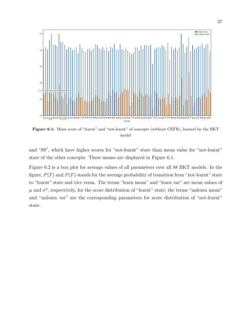
We train 88 BKT models for all concepts. The total time for training all models is ap-proximately 82 seconds, using 4 processors. The mean scores for the “learnt” state for eachconcept are mostly in the interval between 0.75 and 0.85, except concepts labeled “7”, “8”,“191”, “230”, “85” and “89”. The mean scores for the “not-learnt” state are mostly in theinterval between 0.1 and 0.3. There are two significant exceptions, which are concept “85”

37

Figure 6.1: Mean score of “learnt” and “not-learnt” of concepts (without CEFR), learned by the BKTmodel

and “89”, which have higher scores for “not-learnt” state than mean value for “not-learnt”state of the other concepts. These means are displayed in Figure 6.1.

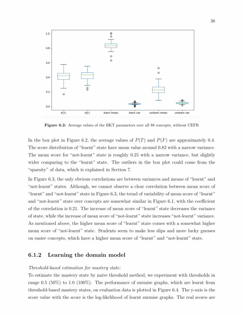
Figure 6.2 is a box plot for average values of all parameters over all 88 BKT models. In thefigure, P (T ) and P (F ) stands for the average probability of transition from “not-learnt” stateto “learnt” state and vice versa. The terms “learn mean” and “learn var” are mean values ofµ and σ2, respectively, for the score distribution of “learnt” state; the terms “unlearn mean”and “unlearn var” are the corresponding parameters for score distribution of “not-learnt”state.

38

Figure 6.2: Average values of the BKT parameters over all 88 concepts, without CEFR

In the box plot in Figure 6.2, the average values of P (T ) and P (F ) are approximately 0.4.The score distribution of “learnt” state have mean value around 0.82 with a narrow variance.The mean score for “not-learnt” state is roughly 0.25 with a narrow variance, but slightlywider comparing to the “learnt” state. The outliers in the box plot could come from the“sparsity” of data, which is explained in Section 7.

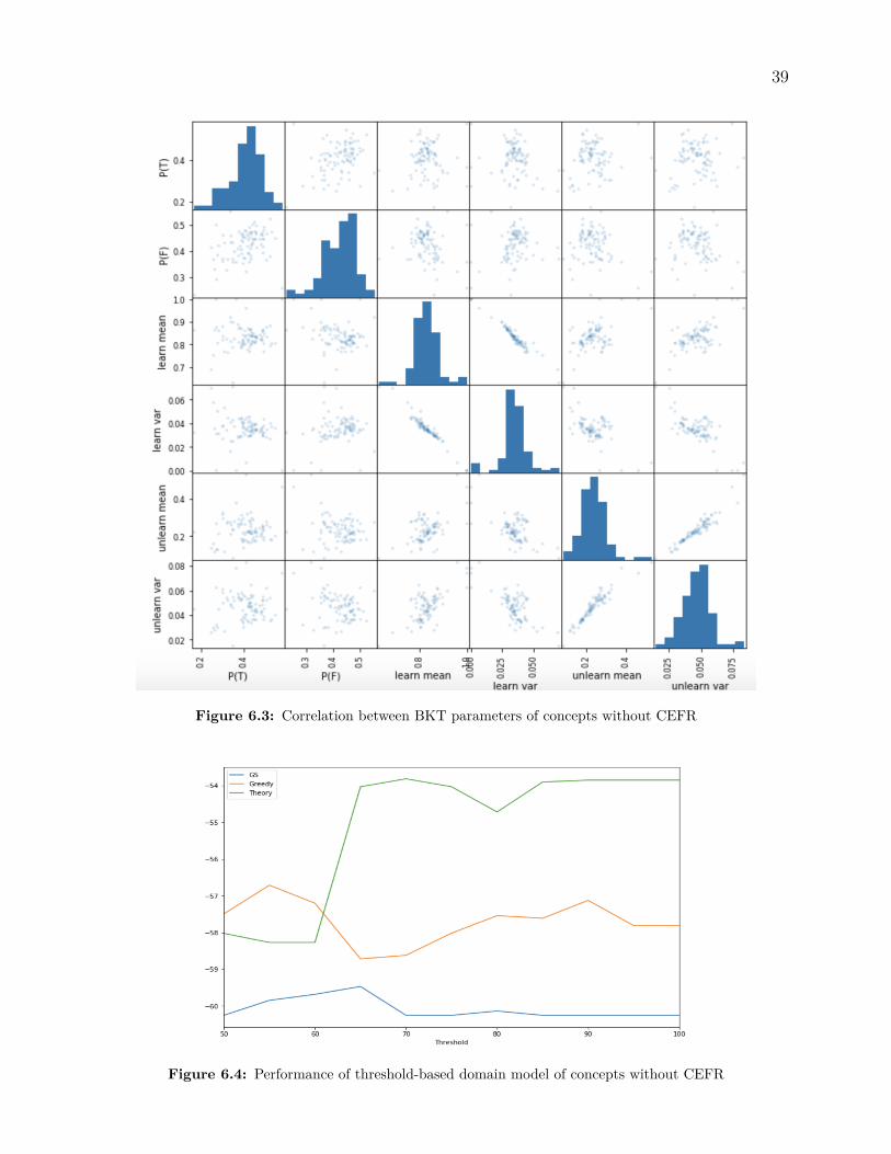
In Figure 6.3, the only obvious correlations are between variances and means of “learnt” and“not-learnt” states. Although, we cannot observe a clear correlation between mean score of“learnt” and “not-learnt” state in Figure 6.3, the trend of variability of mean score of “learnt”and “not-learnt” state over concepts are somewhat similar in Figure 6.1, with the coefficientof the correlation is 0.21. The increase of mean score of “learnt” state decreases the varianceof state, while the increase of mean score of “not-learnt” state increases “not-learnt” variance.As mentioned above, the higher mean score of “learnt” state comes with a somewhat highermean score of “not-learnt” state. Students seem to make less slips and more lucky guesseson easier concepts, which have a higher mean score of “learnt” and “not-learnt” state.

6.1.2 Learning the domain model

Threshold-based estimation for mastery state:To estimate the mastery state by naive threshold method, we experiment with thresholds inrange 0.5 (50%) to 1.0 (100%). The performance of surmise graphs, which are learnt fromthreshold-based mastery states, on evaluation data is plotted in Figure 6.4. The y-axis is thescore value with the score is the log-likelihood of learnt surmise graphs. The real scores are

39

Figure 6.3: Correlation between BKT parameters of concepts without CEFR

Figure 6.4: Performance of threshold-based domain model of concepts without CEFR

40

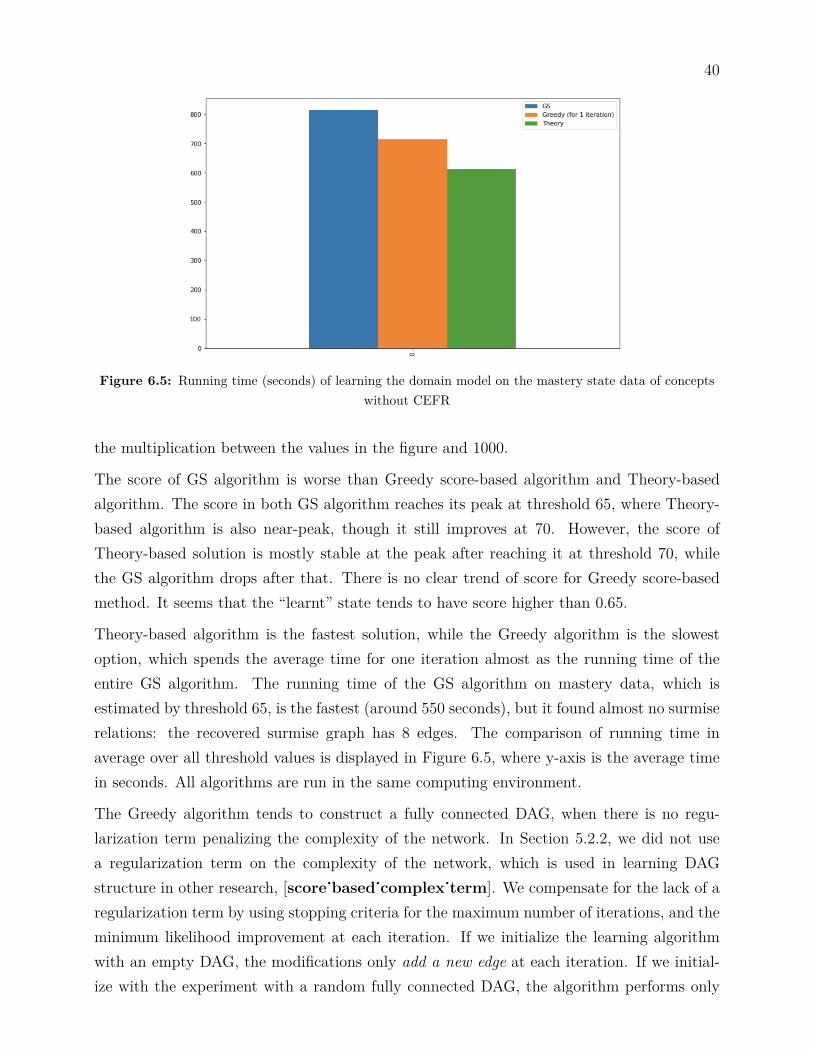
Figure 6.5: Running time (seconds) of learning the domain model on the mastery state data of conceptswithout CEFR

the multiplication between the values in the figure and 1000.

The score of GS algorithm is worse than Greedy score-based algorithm and Theory-basedalgorithm. The score in both GS algorithm reaches its peak at threshold 65, where Theory-based algorithm is also near-peak, though it still improves at 70. However, the score ofTheory-based solution is mostly stable at the peak after reaching it at threshold 70, whilethe GS algorithm drops after that. There is no clear trend of score for Greedy score-basedmethod. It seems that the “learnt” state tends to have score higher than 0.65.

Theory-based algorithm is the fastest solution, while the Greedy algorithm is the slowestoption, which spends the average time for one iteration almost as the running time of theentire GS algorithm. The running time of the GS algorithm on mastery data, which isestimated by threshold 65, is the fastest (around 550 seconds), but it found almost no surmiserelations: the recovered surmise graph has 8 edges. The comparison of running time inaverage over all threshold values is displayed in Figure 6.5, where y-axis is the average timein seconds. All algorithms are run in the same computing environment.

The Greedy algorithm tends to construct a fully connected DAG, when there is no regu-larization term penalizing the complexity of the network. In Section 5.2.2, we did not usea regularization term on the complexity of the network, which is used in learning DAGstructure in other research, [score˙based˙complex˙term]. We compensate for the lack of aregularization term by using stopping criteria for the maximum number of iterations, and theminimum likelihood improvement at each iteration. If we initialize the learning algorithmwith an empty DAG, the modifications only add a new edge at each iteration. If we initial-ize with the experiment with a random fully connected DAG, the algorithm performs only

41

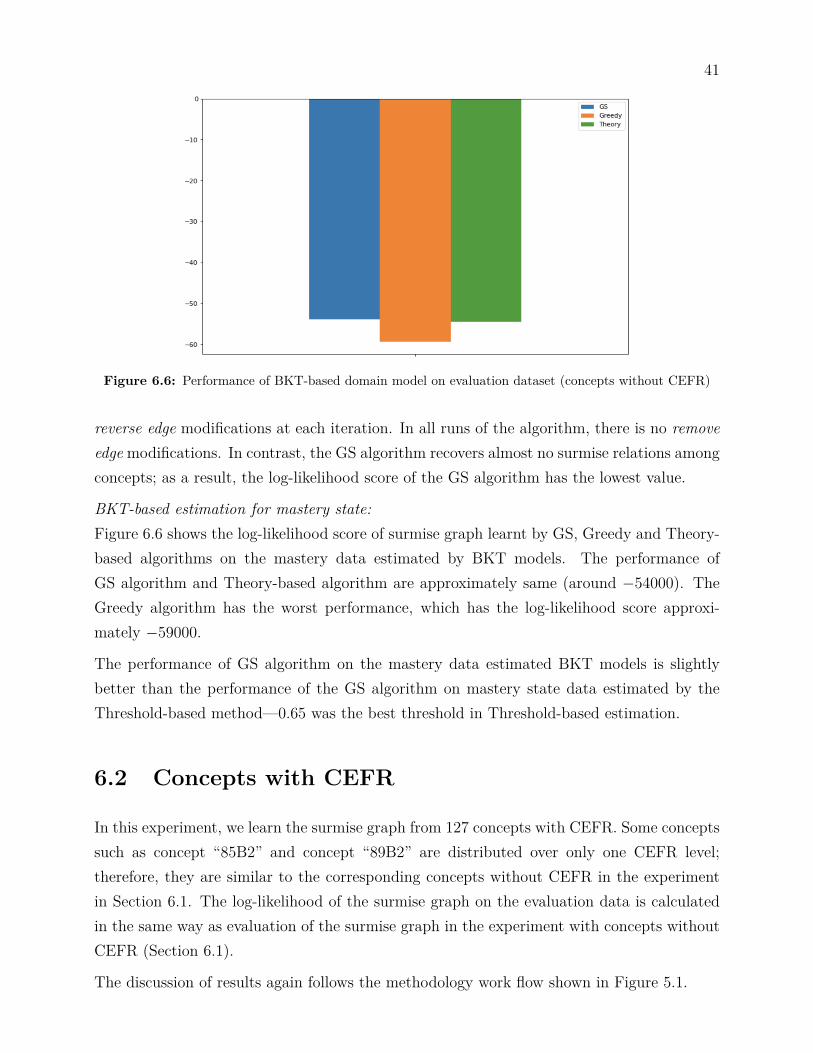
Figure 6.6: Performance of BKT-based domain model on evaluation dataset (concepts without CEFR)

reverse edge modifications at each iteration. In all runs of the algorithm, there is no removeedge modifications. In contrast, the GS algorithm recovers almost no surmise relations amongconcepts; as a result, the log-likelihood score of the GS algorithm has the lowest value.

BKT-based estimation for mastery state:Figure 6.6 shows the log-likelihood score of surmise graph learnt by GS, Greedy and Theory-based algorithms on the mastery data estimated by BKT models. The performance ofGS algorithm and Theory-based algorithm are approximately same (around −54000). TheGreedy algorithm has the worst performance, which has the log-likelihood score approxi-mately −59000.

The performance of GS algorithm on the mastery data estimated BKT models is slightlybetter than the performance of the GS algorithm on mastery state data estimated by theThreshold-based method—0.65 was the best threshold in Threshold-based estimation.

6.2 Concepts with CEFR

In this experiment, we learn the surmise graph from 127 concepts with CEFR. Some conceptssuch as concept “85B2” and concept “89B2” are distributed over only one CEFR level;therefore, they are similar to the corresponding concepts without CEFR in the experimentin Section 6.1. The log-likelihood of the surmise graph on the evaluation data is calculatedin the same way as evaluation of the surmise graph in the experiment with concepts withoutCEFR (Section 6.1).

The discussion of results again follows the methodology work flow shown in Figure 5.1.

42

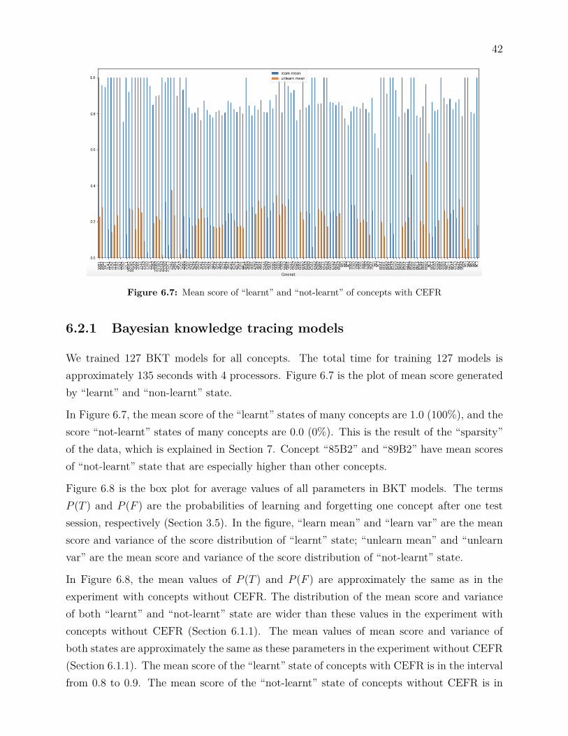
Figure 6.7: Mean score of “learnt” and “not-learnt” of concepts with CEFR

6.2.1 Bayesian knowledge tracing models

We trained 127 BKT models for all concepts. The total time for training 127 models isapproximately 135 seconds with 4 processors. Figure 6.7 is the plot of mean score generatedby “learnt” and “non-learnt” state.

In Figure 6.7, the mean score of the “learnt” states of many concepts are 1.0 (100%), and thescore “not-learnt” states of many concepts are 0.0 (0%). This is the result of the “sparsity”of the data, which is explained in Section 7. Concept “85B2” and “89B2” have mean scoresof “not-learnt” state that are especially higher than other concepts.

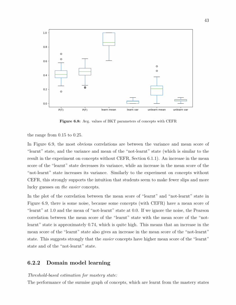
Figure 6.8 is the box plot for average values of all parameters in BKT models. The termsP (T ) and P (F ) are the probabilities of learning and forgetting one concept after one testsession, respectively (Section 3.5). In the figure, “learn mean” and “learn var” are the meanscore and variance of the score distribution of “learnt” state; “unlearn mean” and “unlearnvar” are the mean score and variance of the score distribution of “not-learnt” state.

In Figure 6.8, the mean values of P (T ) and P (F ) are approximately the same as in theexperiment with concepts without CEFR. The distribution of the mean score and varianceof both “learnt” and “not-learnt” state are wider than these values in the experiment withconcepts without CEFR (Section 6.1.1). The mean values of mean score and variance ofboth states are approximately the same as these parameters in the experiment without CEFR(Section 6.1.1). The mean score of the “learnt” state of concepts with CEFR is in the intervalfrom 0.8 to 0.9. The mean score of the “not-learnt” state of concepts without CEFR is in

43

Figure 6.8: Avg. values of BKT parameters of concepts with CEFR

the range from 0.15 to 0.25.

In Figure 6.9, the most obvious correlations are between the variance and mean score of“learnt” state, and the variance and mean of the “not-learnt” state (which is similar to theresult in the experiment on concepts without CEFR, Section 6.1.1). An increase in the meanscore of the “learnt” state decreases its variance, while an increase in the mean score of the“not-learnt” state increases its variance. Similarly to the experiment on concepts withoutCEFR, this strongly supports the intuition that students seem to make fewer slips and morelucky guesses on the easier concepts.

In the plot of the correlation between the mean score of “learnt” and “not-learnt” state inFigure 6.9, there is some noise, because some concepts (with CEFR) have a mean score of“learnt” at 1.0 and the mean of “not-learnt” state at 0.0. If we ignore the noise, the Pearsoncorrelation between the mean score of the “learnt” state with the mean score of the “not-learnt” state is approximately 0.74, which is quite high. This means that an increase in themean score of the “learnt” state also gives an increase in the mean score of the “not-learnt”state. This suggests strongly that the easier concepts have higher mean score of the “learnt”state and of the “not-learnt” state.

6.2.2 Domain model learning

Threshold-based estimation for mastery state:The performance of the surmise graph of concepts, which are learnt from the mastery states

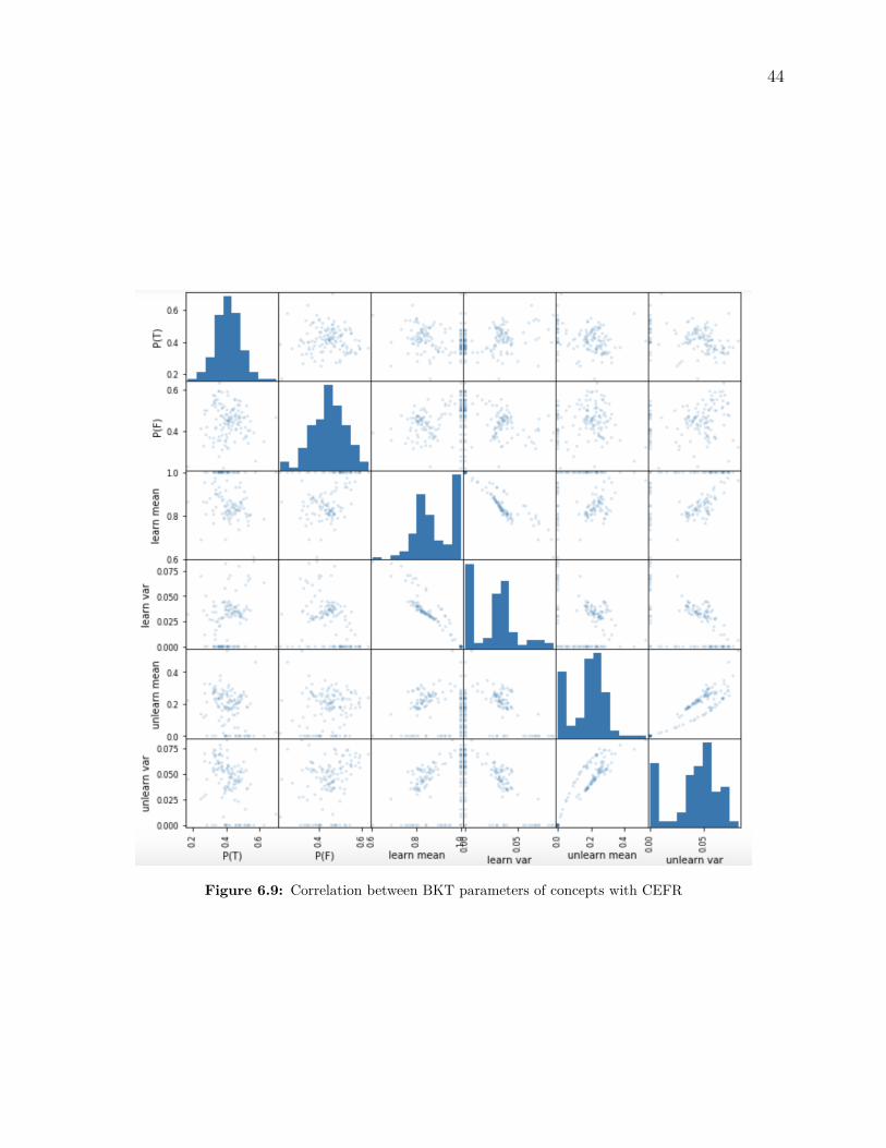
44

Figure 6.9: Correlation between BKT parameters of concepts with CEFR

45

Figure 6.10: Performance of threshold-based domain model of concepts with CEFR

by Threshold-based estimator is plotted in Figure 6.10. In the figure, the x-axis shows thevalues of thresholds and y-axis shows the log-likelihoods (the y-values are the log-likelihoodsdivided by 1000) of the surmise graphs on the evaluation dataset. We tried thresholds inrange 0.5 (50%) to 1.0 (100%). The general performance of the GS, Theory-based and Greedyscore-based algorithms on the mastery states from the Threshold-based estimator in theexperiment on concepts with CEFR have higher average log-likelihoods than in experimenton concepts without CEFR (comparing Figure 6.10 and Figure 6.4).

In Figure 6.10, the general performance of the Theory-based method on the mastery data,from the Threshold-based estimator, is better than the GS and Greedy method. The perfor-mance of the GS algorithm and Theory-based method have a similar trend, which increasesstrongly from about threshold 50 to 70 or 75 then is stable from threshold 75 to 100. Thisshows that the threshold 70 or 75 seems to be the most probable mastery threshold. Thismeans that students who learnt skill A tend to have scores for skill A higher than 0.70 or0.75.

The GS algorithm is the fastest, which is four times faster than the Theory-based algorithmand hundreds of times faster than the Greedy score-based algorithm. The details of runningtime is presented in Figure 6.11, where the running time is given on the y-axis in seconds.

BKT-based estimation for mastery state:Figure 6.12, shows the comparison between the performance of the GS, Greedy and Theory-based algorithms on the mastery data that is estimated by BKT models. The y-axis is thelog-likelihood (divided by 1000) of the surmise graphs obtained from the mastery data. TheGS algorithm is the winner with the highest log-likelihood, −22000, and the Theory-basedalgorithm is the much worse, with the log-likelihood almost −49000. The log-likelihood of

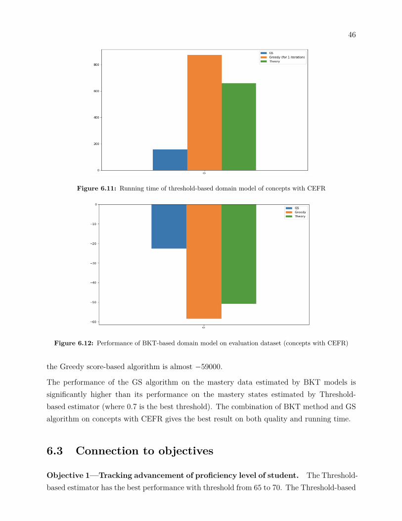
46

Figure 6.11: Running time of threshold-based domain model of concepts with CEFR

Figure 6.12: Performance of BKT-based domain model on evaluation dataset (concepts with CEFR)

the Greedy score-based algorithm is almost −59000.

The performance of the GS algorithm on the mastery data estimated by BKT models issignificantly higher than its performance on the mastery states estimated by Threshold-based estimator (where 0.7 is the best threshold). The combination of BKT method and GSalgorithm on concepts with CEFR gives the best result on both quality and running time.

6.3 Connection to objectives

Objective 1—Tracking advancement of proficiency level of student. The Threshold-based estimator has the best performance with threshold from 65 to 70. The Threshold-based

47

estimator is able to extract the probability that a student with “learnt” state makes slips.The Threshold-based estimator is decent to estimate the proficiency level of students basedon their scores, however, the Threshold-based estimator is not able to track the advance-ment, which contains the probabilities of learning and forgetting. On the other hand, theBKT models can extract both the probabilities of making slips and lucky guesses, and theprobabilities of learning and forgetting. BKT models is able to predict the future scoresbased on the historical performance, while the Threshold-based estimator is not able to doso.

Objective 2—Measuring the difficulty of concepts. BKT models is able to extractthe correlation between “learn” and “not-learnt” state, and the correlation between the meanof score and the variance of score. The variance of score can tell us the probabilities of luckyguesses and slips. The positive correlation between mean score of “learnt” state and meanscore of “not-learnt” state derives that harder concepts tend to have higher score with bothstates. The correlation between mean score and score variance derives the changes of theprobabilities of making slips and lucky guesses according to the hardness of concepts. Bythe experiment results, students seem to make more lucky guesses and fewer slips at easierconcepts.

Objective 3—Proposing learning plans for students. The student model is able toestimate the current knowledge state of a students. The domain model can detect thatcurrent knowledge state in the surmise graph and find the optimal learning curve to helpthe student achieve the study target. Refining concepts with the CEFR levels boosts theperformance of learnt domain model, which means that the surmise graph of concepts withCEFR seem to be the better guideline of learning curve for students. The Theory-basedalgorithm has a drawback that this algorithm seems to be not able to distinguish easierconcepts and prerequisite concepts. Theory-based algorithm learns that the concept “85—Place of adverbs of time, place and manner” and “89—Place of pronouns in a phrase” are theprerequisite concepts for the others, which seems to be not realistic. GS algorithm extractsbetter surmise graph with more sensible points. For example, the GS algorithm learnt thatconcept “24B1—Expressions of time, place and manner. Preposition-free expressions” isthe prerequisite of concept “85B2—Place of adverbs of time, place and manner”, which isreasonable (Figure B.1). Figure B.1 presents the learnt surmise with the best performanceon evaluation data, which is learnt by GS algorithm on the mastery data estimated by BKTmodels on concepts with CEFR.

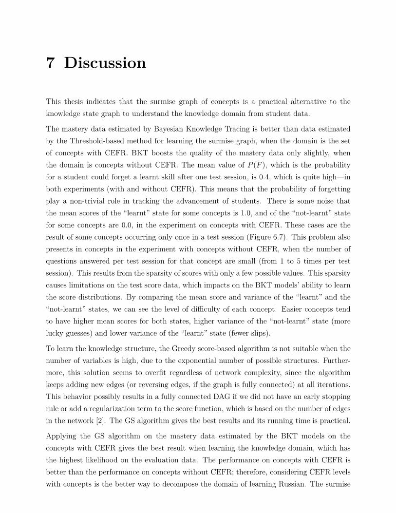
7 Discussion

This thesis indicates that the surmise graph of concepts is a practical alternative to theknowledge state graph to understand the knowledge domain from student data.

The mastery data estimated by Bayesian Knowledge Tracing is better than data estimatedby the Threshold-based method for learning the surmise graph, when the domain is the setof concepts with CEFR. BKT boosts the quality of the mastery data only slightly, whenthe domain is concepts without CEFR. The mean value of P (F ), which is the probabilityfor a student could forget a learnt skill after one test session, is 0.4, which is quite high—inboth experiments (with and without CEFR). This means that the probability of forgettingplay a non-trivial role in tracking the advancement of students. There is some noise thatthe mean scores of the “learnt” state for some concepts is 1.0, and of the “not-learnt” statefor some concepts are 0.0, in the experiment on concepts with CEFR. These cases are theresult of some concepts occurring only once in a test session (Figure 6.7). This problem alsopresents in concepts in the experiment with concepts without CEFR, when the number ofquestions answered per test session for that concept are small (from 1 to 5 times per testsession). This results from the sparsity of scores with only a few possible values. This sparsitycauses limitations on the test score data, which impacts on the BKT models’ ability to learnthe score distributions. By comparing the mean score and variance of the “learnt” and the“not-learnt” states, we can see the level of difficulty of each concept. Easier concepts tendto have higher mean scores for both states, higher variance of the “not-learnt” state (morelucky guesses) and lower variance of the “learnt” state (fewer slips).

To learn the knowledge structure, the Greedy score-based algorithm is not suitable when thenumber of variables is high, due to the exponential number of possible structures. Further-more, this solution seems to overfit regardless of network complexity, since the algorithmkeeps adding new edges (or reversing edges, if the graph is fully connected) at all iterations.This behavior possibly results in a fully connected DAG if we did not have an early stoppingrule or add a regularization term to the score function, which is based on the number of edgesin the network [2]. The GS algorithm gives the best results and its running time is practical.

Applying the GS algorithm on the mastery data estimated by the BKT models on theconcepts with CEFR gives the best result when learning the knowledge domain, which hasthe highest likelihood on the evaluation data. The performance on concepts with CEFR isbetter than the performance on concepts without CEFR; therefore, considering CEFR levelswith concepts is the better way to decompose the domain of learning Russian. The surmise

49

graph, which is obtained by GS algorithm with the mastery data estimated by BKT modelon the concepts with CEFR is presented in Figure B.1 (Appendix B).

It is interesting to compare our results with results presented in paper “Modeling languagelearning using specialized Elo ratings” [12]. That paper reports two knowledge graphs learnedby different techniques. We find some similar points between our graph and their graph. Forexample, we observe that concepts “10”, “11” and “12” are positioned very low in all graphs,meaning that they have few prerequisites, and are prerequisite to many other concepts.Similarly concept “85” is a basic concept (having no children/prerequisites) in all of thesegraphs as well. This kind agreement makes us hopeful that these methods are learning somefundamental properties of the domain.

In the scope of this paper, we have not considered the frequencies of response patterns. Fur-thermore, assuming that P (T ) and P (F ) are constant over time is not realistic. For example,the probability of forgetting a skill, which a student has mastered over many consecutive testsessions should not be not the same as for a student who just mastered it over one testsession; we would expect that

P (Fk|Sk−1 = 1, Sk−2 = 1, Sk−3 = 1) < P (Fk|Sk−1 = 1, Sk−2 = 0, Sk−3 = 0).

In future research, we will attempt to take into account the frequency into our solution,as well as experiment with shifting of P (T ) and P (F ) in BKT models over time. We willalso consider solutions to enhance the quality of the data with larger number of answeredquestions for each concept per test session. The data we used was collected last year, andthe Revita platform accumulates more data over time. We believe that the results presentedin this thesis can be improved with more data, which would reduce the data sparsenessproblems. The quality of the models can be further evaluated by actual users. We canmeasure the performance of the advancement prediction as well as the satisfaction of userson the guideline of learning curve learnt from the domain model.

8 Conclusions

This thesis presents the adaption of Bayesian knowledge tracing model to tracking student’sadvancement in language learning, as well as the application of the Grow-shrink Markovblanket algorithm, Greedy score-based algorithm and Theory-driven algorithm to learn thenetwork structure for the knowledge domain, based on data from students learning Russian.The result indicates the effectiveness of the BKT model in order to estimate students’ masterystate on every skill and of the GS algorithm on recovering the domain structure. We learnthe surmise relation among concepts and build a compete network of concepts in the domain.

These surmise connections can be used as guideline for the students to improve the learningcurve, while the tracing model can be used to estimate the proficiency levels of studentsover their test results. The experiments also suggest that decomposing the domain into finerconcepts based on their CEFR levels is more effective than ignoring the CEFR levels.

Future research will be focused on extending the BKT model with the flexible probabilitiesfor learning and forgetting a skill, as well as considering the frequency factor of knowledgestates. Furthermore, we will try to accumulate more data with high diversity in order tohave better experiments.

Acknowledgement

We would like to thank the team of the Revita Project, which conducts research on languagelearning systems, at the Department of Computer Science, Department of Digital Humanities,and the Department of Modern Languages, University of Helsinki, for their data and supportin completing this research project.

Bibliography

[1] D. Albert & J. Lukas. Knowledge Spaces: Theories, Empirical Research, Applications.Lawrence Erlbaum Associates, 1999.

[2] S. Beretta, M. Castelli, I. Goncalves, R. Henriques & D. Ramazzotti. “Learning thestructure of Bayesian Networks: A quantitative assessment of the effect of differentalgorithmic schemes”. In: Complexity 2018 (2018).

[3] G. F. Cooper & E. Herskovits. “A Bayesian method for the induction of probabilisticnetworks from data”. In: Machine Learning 9 (1992), pp. 309–347. doi: 10.1007/

BF00994110.

[4] A. T. Corbett & J. Anderson. “Knowledge tracing: Modeling the acquisition of proce-dural knowledge”. In: User Modeling and User-Adapted Interaction 4 (1994), pp. 253–278. doi: 10.1007/BF01099821.

[5] J. Cussens & M. Bartlett. GOBNILP 1.6.2 User/Developer Manual. University of York,2015.

[6] M. Desmarais & M. Gagnon. “Bayesian Student Models Based on Item to Item Knowl-edge Structures”. In: European Conference on Technology Enhanced Learning. 2006,pp. 111–124. doi: 10.1007/11876663_11.

[7] J.-P. Doignon & J.-C. Falmagne. Knowledge Spaces. Berlin: Springer-Verlag, 1999.

[8] J.-P. Doignon & J.-C. Falmagne. “Knowledge spaces and learning spaces”. In: Newhandbook of mathematical psychology 2 (2016), pp. 274–321.

[9] J.-P. Doignon & J.-C. Falmagne. “Spaces for the assessment of knowledge”. In: In-ternational Journal of Man-Machine Studies 23.2 (August 1985), pp. 175–196. doi:10.1016/S0020-7373(85)80031-6.

[10] J.-C. Falmagne, D. Albert, C. Doble, D. Eppstein & X. Hu, eds. Knowledge spaces.Applications in education. 2013. doi: 10.1007/978-3-642-35329-1.

[11] P. A. Gagniuc. Markov Chains: From Theory to Implementation and Experimentation.Hoboken, NJ : John Wiley & Sons, 2017.

52

[12] J. Hou, K. Maximilian, J. M. Hoya Quecedo, N. Stoyanova & R. Yangarber. “Modelinglanguage learning using specialized Elo rating”. In: Proceedings of the Fourteenth Work-shop on Innovative Use of NLP for Building Educational Applications. Florence, Italy:Association for Computational Linguistics, 2019, pp. 494–506. doi: 10.18653/v1/W19-

4451.

[13] A. Katinskaia, J. Nouri & R. Yangarber. “Revita: a language-learning platform at theintersection of ITS and CALL”. In: Proceedings of LREC: 11th International Conferenceon Language Resources and Evaluation. Miyazaki, Japan, 2018.

[14] D. Margaritis. “Learning Bayesian Network Model Structure from Data”. PhD thesis.Pittsburgh, PA 15213: Carnegie Mellon University, 2003.

[15] J. Pearl. “Causal Diagrams for Empirical Research”. In: Biometrika 82.4 (1995), pp. 669–688. doi: 10.2307/2337329.

[16] J. Pearl. Causality. Cambridge University Press, 2009. doi: 10.1017/CBO9780511803161.

[17] J. Pearl. Probabilistic reasoning in intelligent systems: Networks of Plausible Inference.Morgan Kaufmann Publishers, San Francisco, CA, United States, 1988.

[18] J. Pearl & T. S.Verma. “A theory of inferred causation”. In: Studies in Logic and theFoundations of Mathematics 134 (1995), pp. 789–811. doi: 10.1016/S0049-237X(06)

80074-1.

[19] E. Robusto & L. Stefanutti. “Extracting a knowledge structure from the data by a max-imum residuals method”. In: TPM - Testing, Psychometrics, Methodology in AppliedPsychology 21 (2014), pp. 421–433. doi: 10.4473/TPM21.4.4.

[20] B. V. de Sande. “Properties of the Bayesian Knowledge Tracing Model”. In: EducationalData Mining 5.2 (2013), pp. 253–278. doi: 10.5281/zenodo.3554629.

[21] J. Schreiber. “pomegranate: Fast and Flexible Probabilistic Modeling in Python”. In:Machine Learning Research 18 (2018).

[22] M. Schrepp. “A method for the analysis of hierarchical dependencies between items ofa questionnaire”. In: Methods of Psychological Research Online 8 (2003), pp. 43–79.

[23] M. Schrepp. “Extracting knowledge structures from observed data”. In: British Journalof Mathematical and Statistical Psychology 52 (1999), pp. 213–224. doi: 10.1348/

000711099159071.

[24] P. Spirtes, C. Glymour & R. Scheines. Causation, Prediction, and Search. 1993. doi:10.1007/978-1-4612-2748-9.

53

[25] A. Spoto, L. Stefanutti & G. Vidotto. “Knowledge space theory, formal concept anal-ysis, and computerized psychological assessment”. In: Behavior Research Methods 42.1(February 2010), pp. 342–350. doi: 10.3758/BRM.42.1.342.

[26] L. Stefanutti, D. Albert & C. Hockemeyer. “Derivation of Knowledge Structures forDistributed Learning Objects”. In: Cognitive Science Section (2003).

[27] A. Tandon & S. Soni. Introduction to Artificial Intelligence using Python. Book BazookaPublication, 2020. url: https://books.google.fi/books?id=ExTNDwAAQBAJ.

[28] C. Yuan & B. Malone. “Learning Optimal Bayesian Networks: A Shortest Path Per-spective”. In: Journal of Artificial Intelligence Research 48 (2013), pp. 23–65.

[29] K. Zhanga & Y. Yao. “A three learning states Bayesian knowledge tracing model”. In:Knowledge-Based Systems 148 (2018), pp. 189–201.

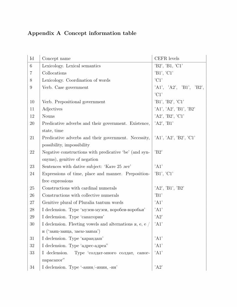
Appendix A Concept information table

Id Concept name CEFR levels

6 Lexicology. Lexical semantics ’B2’, ’B1, ’C1’7 Collocations ’B1’, ’C1’8 Lexicology. Coordination of words ’C1’9 Verb. Case government ’A1’, ’A2’, ’B1’, ’B2’,

’C1’10 Verb. Prepositional government ’B1’, ’B2’, ’C1’11 Adjectives ’A1’, ’A2’, ’B1’, ’B2’12 Nouns ’A2’, ’B2’, ’C1’20 Predicative adverbs and their government. Existence,

state, time’A2’, ’B1’

21 Predicative adverbs and their government. Necessity,possibility, impossibility

’A1’, ’A2’, ’B2’, ’C1’

22 Negative constructions with predicative ‘be’ (and syn-onyms), genitive of negation

’B2’

23 Sentences with dative subject: ‘Кате 25 лет’ ’A1’24 Expressions of time, place and manner. Preposition-

free expressions’B1’, ’C1’

25 Constructions with cardinal numerals ’A2’, ’B1’, ’B2’26 Constructions with collective numerals ’B1’27 Genitive plural of Pluralia tantum words ’A1’28 I declension. Type ‘музеи-музеи, воробеи-воробьи’ ’A1’29 I declension. Type ‘санатории’ ’A2’30 I declension. Fleeting vowels and alternations я, е, е /

и (‘заяц-заица, заем-заима’)’A1’

31 I declension. Type ‘карандаш’ ’A1’32 I declension. Type ‘адрес-адреа” ’A1’33 I declension. Type ‘солдат-много солдат, сапог-

парасапог”’A1’

34 I declension. Type ‘-анин/-янин, -ин’ ’A2’

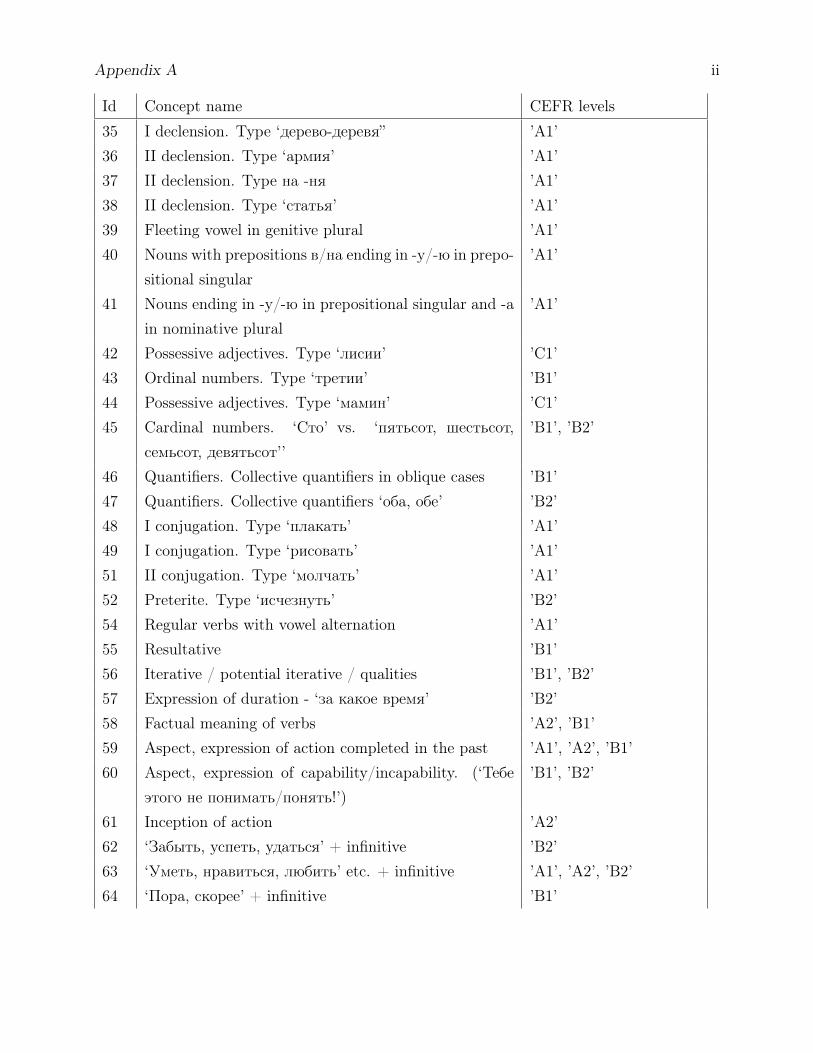
Appendix A ii

Id Concept name CEFR levels

35 I declension. Type ‘дерево-деревя” ’A1’36 II declension. Type ‘армия’ ’A1’37 II declension. Type на -ня ’A1’38 II declension. Type ‘статья’ ’A1’39 Fleeting vowel in genitive plural ’A1’40 Nouns with prepositions в/на ending in -у/-ю in prepo-

sitional singular’A1’

41 Nouns ending in -у/-ю in prepositional singular and -аin nominative plural

’A1’

42 Possessive adjectives. Type ‘лисии’ ’C1’43 Ordinal numbers. Type ‘третии’ ’B1’44 Possessive adjectives. Type ‘мамин’ ’C1’45 Cardinal numbers. ‘Сто’ vs. ‘пятьсот, шестьсот,

семьсот, девятьсот’’’B1’, ’B2’

46 Quantifiers. Collective quantifiers in oblique cases ’B1’47 Quantifiers. Collective quantifiers ‘оба, обе’ ’B2’48 I conjugation. Type ‘плакать’ ’A1’49 I conjugation. Type ‘рисовать’ ’A1’51 II conjugation. Type ‘молчать’ ’A1’52 Preterite. Type ‘исчезнуть’ ’B2’54 Regular verbs with vowel alternation ’A1’55 Resultative ’B1’56 Iterative / potential iterative / qualities ’B1’, ’B2’57 Expression of duration - ‘за какое время’ ’B2’58 Factual meaning of verbs ’A2’, ’B1’59 Aspect, expression of action completed in the past ’A1’, ’A2’, ’B1’60 Aspect, expression of capability/incapability. (‘Тебе

этого не понимать/понять!’)’B1’, ’B2’

61 Inception of action ’A2’62 ‘Забыть, успеть, удаться’ + infinitive ’B2’63 ‘Уметь, нравиться, любить’ etc. + infinitive ’A1’, ’A2’, ’B2’64 ‘Пора, скорее’ + infinitive ’B1’

Appendix A iii

Id Concept name CEFR levels

65 ‘Нельзя, невозможно, не могу’ + infinitive ’A1’, ’A2’66 ‘Не’ + infinitive ’B2’67 Negative sentences ’A2’68 Imperative ’A1’69 Proximal future ’A2’70 Impersonal sentences. Infinitival sentences. Subordi-

nate sentences (‘если / прежде чем’ + infinitive)’B2’

72 Impersonal sentences. Infinitival sentences. Sentences,with negative pronouns and adverbs

’B2’

73 Generis-personal sentences ’B2’75 Passive and its relation to indefinite-personal sentences

(equivalent of Finnish impersonal passive)’B1’

76 Stress: forms of verbal preterite ’B2’77 Stress: short adjectives ’B2’78 Stress: participles ’B2’79 Nouns. Type A: stress on the stem ’A1’80 Nouns. Type B, B1, B2: stress on the ending ’A1’, ’B1’, ’B2’81 Nouns. Type C, C1: stress on the stem in singular, on

the ending in plural’A1’, ’A2’, ’B2’

82 Nouns. Type D, D1: stress on the ending in singular,on the stem in plural

’A1’, ’B1’

83 Nouns. Type ‘нож-ножом, сторож-сторожем’ ’A1’84 Declension of adjectives. Type ‘хорошего’ ’A1’85 Place of adverbs of time, place and manner ’B2’86 Place of negation in the sentence ’B1’, ’C1’87 Place of participles in the sentence ’B1’88 Place of gerunds in the sentence ’B1’89 Place of pronouns in a phrase ’B2’90 Word order in sentences introducing direct quotations ’C1’91 Second person singular imperative in conditionals

(‘если’)’B2’

92 Usage of ‘сам’ and ’один’ ’B2’93 Sentences of type ‘Знаю его как врача ’B1’, ’B2’

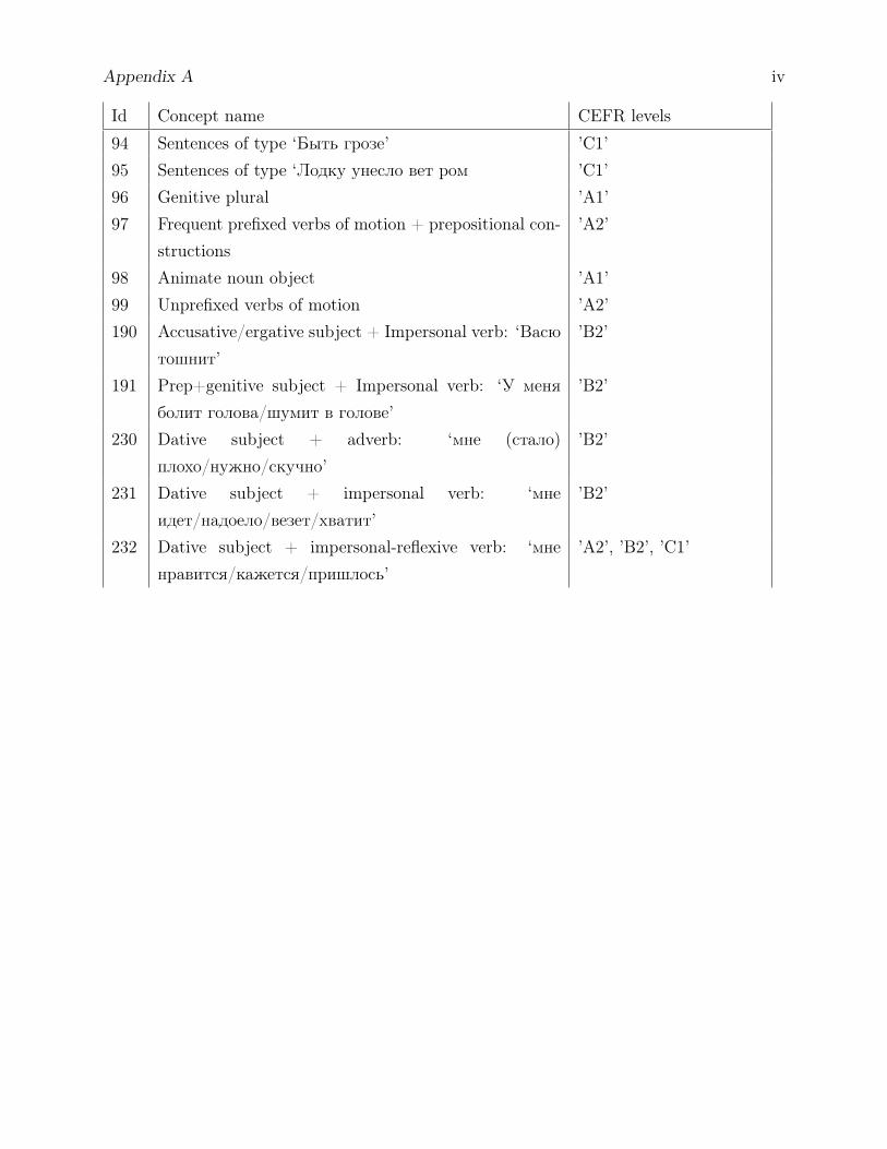
Appendix A iv

Id Concept name CEFR levels

94 Sentences of type ‘Быть грозе’ ’C1’95 Sentences of type ‘Лодку унесло вет ром ’C1’96 Genitive plural ’A1’97 Frequent prefixed verbs of motion + prepositional con-

structions’A2’

98 Animate noun object ’A1’99 Unprefixed verbs of motion ’A2’190 Accusative/ergative subject + Impersonal verb: ‘Васю

тошнит’’B2’

191 Prep+genitive subject + Impersonal verb: ‘У меняболит голова/шумит в голове’

’B2’

230 Dative subject + adverb: ‘мне (стало)плохо/нужно/скучно’

’B2’

231 Dative subject + impersonal verb: ‘мнеидет/надоело/везет/хватит’

’B2’

232 Dative subject + impersonal-reflexive verb: ‘мненравится/кажется/пришлось’

’A2’, ’B2’, ’C1’

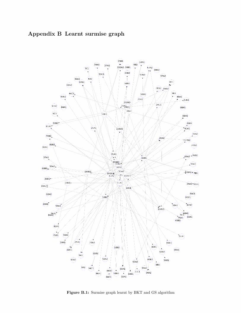
Appendix B Learnt surmise graph

Figure B.1: Surmise graph learnt by BKT and GS algorithm

Appendix B ii

Figure B.1 is the learnt surmise graph with the best performance on the evaluation data.This graph is learnt by applying Grow-Shrink Markov blanket algorithm on the mastery data,which is estimated by the Bayesian Knowledge Tracing models.

In Figure B.1, the arrows present for the surmise relationship, where A→ B means A shouldbe learnt before B. The concepts in the middle area are more likely to be the base conceptsfor the others.