Modeling land-use change and future deforestation in two ... · Modeling land-use change and future deforestation in two spatial scales ... Modeling land-use change and future deforestation

Modeling land-use change and future deforestation in two spatial scalesModelaje del cambio de uso del suelo y la deforestación futura en dos escalas espaciales

Carmina Cruz-Huerta1; Manuel J. González-Guillén1*; Tomás Martínez-Trinidad1; Miguel J. Escalona-Maurice2

1Postgrado en Ciencias Forestales, 2Desarrollo Rural, Colegio de Postgraduados. Carretera México-Texcoco

km 36.5. C. P. 56230. Montecillo, Texcoco, Edo. de México. Correo-e: [email protected] Tel.: 595 95 202 00

ext. 1464 (*Autor para correspondencia).

Abstract

Land-use changes in the Chignahuapan-Zacatlán region of the state of Puebla, Mexico, and in each of the two aforementioned counties, were determined using Landsat imagery and a bitemporal analysis of the period 1986-2011. The predominant land uses

at the regional level are the agricultural (49.7 %) and forest (46.1) groupings. In the case of Chignahuapan county, agricultural use is the main activity with 58.9 % of the territory, while in Zacatlán county the predominant activity is forest use with 57.3 % of the land base. At the regional level and for Zacatlán county, the probabilistic model of forest land-use change was significantly correlated (P ≤ 0.05) with 21 independent variables; however, for Chignahuapan, the model only considered 16 variables. At the regional level, the probability of forest land changing to other uses ranged from 5-90 % and at the county level from 7-99.8 %. Finally, the projection for the year 2030 estimates that the deforestation risk at the regional level and in Chignahuapan and Zacatlán counties is 13,063.8, 10,966.6 and 4,405.5 ha, respectively.

Resumen

En este estudio se determinó el cambio de uso de suelo en la región de Chignahuapan-Zacatlán, Puebla, mediante un análisis bitemporal entre 1986 y 2011; la evaluación se hizo también para cada municipio. El cambio de uso de suelo se detectó mediante el

manejo de imágenes Landsat. Los usos predominantes a nivel regional son el agrícola (49.7 %) y el forestal (46.1 %). En el caso de Chignahuapan, el uso agrícola representa la actividad principal con 58.9 % del territorio, mientras que en Zacatlán predomina el uso forestal con 57.3 %. A nivel regional y para el municipio de Zacatlán, el cambio de uso del suelo forestal se correlacionó significativamente (P ≤ 0.05) con 21 variables independientes, mediante un modelo probabilístico; en el caso de Chignahuapan, el modelo consideró 16 variables. A nivel regional, la probabilidad de cambio de uso de suelo forestal varió de 5 a 90 % y a nivel municipal de 7 a 99.8 %. Finalmente, la proyección para el año 2030 estima que el riesgo de deforestación a nivel regional y en los municipios de Chignahuapan y Zacatlán será de 13,063.8, 10,966.6 y 4,405.5 ha, respectivamente.

Received: June 5, 2014 / Accepted: April 24, 2015.

Palabras clave: Patrones de deforestación,

Chignahuapan, Zacatlán, usos del suelo.

Keywords: Deforestation patterns, Chignahuapan,

Zacatlán, land uses.

Please cite this article as follows (APA6): Cruz-Huerta, C., González-Guillén, M. J., Martínez-Trinidad, T., & Escalona-Maurice, M. J. (2015). Modeling land-use change and future deforestation in two spatial scales. Revista Chapingo Serie Ciencias Forestales y del Ambiente, 21 (2), 137–156. doi: 10.5154/r.rchscfa.2014.06.025

Scientific article doi: 10.5154/r.rchscfa.2014.06.025

www.chapingo.mx/revistas/forestales

138 Spatial analysis of future deforestation

Revista Chapingo Serie Ciencias Forestales y del Ambiente | Vol. XXI, núm. 2, mayo-agosto 2015.

Introduction

Deforestation is a process of change in land cover and use from natural vegetation to residential, agricultural, livestock, industrial or commercial uses (Evangelista, López, Caballero, & Martínez, 2010; Rosete, Pérez, & Bocco, 2008) at different spatial-temporal scales (Gomben, Lilieholm, & González-Guillen, 2012; Hunter et al., (2003). Deforestation has a direct impact on the reduction and fragmentation of forest ecosystems by negatively modifying their structure and functioning. The impacts of deforestation alter the natural capital (Sarukhán, Carabias, Koleff, & Urquiza-Haas, 2012) and its ability to meet human needs (Vitousek, Mooney, Lubchenco, & Melillo, 1997). Changes in land cover and use also determine, in part, the vulnerability of people and places to climatic, economic and socio-political disturbances. When these changes are aggregated globally, they affect central aspects of earth system functioning (Lambin, Geist, & Lepers, 2003).

Understanding the impact caused by changes in land cover and use means studying natural, social, cultural and institutional aspects; however, in Mexico there are few studies (Rosete et al., 2008) that provide a quantitative analysis of the relative importance of these aspects, so interpretations of how these factors interact to induce this change vary widely from one place to another (Skole, Chomentowski, Salas, & Nobre, 1994). Therefore, the impact of change in land cover and use should be analyzed under different spatial scales (O’Neill, 1989), for example at the village, town, city, county, region, state or country level. Each spatial scale represents an appropriate and unique approach to certain factors of interest (Alcaraz, Bandi, & Garbulsky, 2008; Bocco, Mendoza, & Masera, 2001). The information generated is essential for developing effective public policies related to land-use planning.

Several studies have modeled and analyzed the deforestation process at the regional level using small scales and considering socioeconomic and environmental variables (Bocco et al., 2001; Chaves & Rosero-Bixby, 2001; Pineda, Bosques, Gómez, & Plata, 2009). In general, studies at small scales are associated with large units of analysis (region, state, country) and vice versa; however, there are exceptions depending on the level of precision of the analysis. For example, the Instituto Nacional de Ecología y Cambio Climático (INECC, 2011), Mexico’s National Institute of Ecology and Climate Change, determined the national deforestation risk index considering only the national economic pressure index. The study notes that the state of Puebla has an average deforestation rate of 3.3 %, equivalent to 15,000 ha·yr-1; however, one possible downside to this study was the resolution used (9-ha cells). To avoid this, some authors like Alcaraz et al. (2008) and Trucíos, Rivera, Delgado, Estrada, and Cerano (2013) have

Introducción

La deforestación es un proceso de cambio de cobertura y uso de suelo de vegetación natural a residencial, agrícola, pecuario, industrial o comercial (Evangelista, López, Caballero, & Martínez, 2010; Rosete, Pérez, & Bocco, 2008) a diferentes escalas espacio-temporales (Gomben, Lilieholm, & González-Guillen, 2012; Hunter, et al., & Cablk 2003). La deforestación influye directamente en la reducción y fragmentación de los ecosistemas forestales modificando su estructura y funcionamiento negativamente. Los impactos de la deforestación alteran el capital natural (Sarukhán, Carabias, Koleff, & Urquiza-Haas, 2012) y su habilidad para satisfacer necesidades humanas (Vitousek, Mooney, Lubchenco, & Melillo, 1997). Los cambios de cobertura y uso del suelo también determinan, en parte, la vulnerabilidad de lugares y personas ante perturbaciones climáticas, económicas y sociopolíticas. Cuando estos cambios se agregan globalmente afectan aspectos importantes del funcionamiento del sistema Tierra (Lambin, Geist, & Lepers, 2003).

La comprensión del impacto que ocasiona el cambio de cobertura y uso del suelo significa estudiar aspectos naturales, sociales, culturales e institucionales; sin embargo, en México existen pocos estudios (Rosete et al., 2008) sobre el análisis cuantitativo de la importancia relativa de dichos aspectos, por lo que las interpretaciones de cómo estos factores interactúan para inducir ese cambio varían ampliamente de un lugar a otro (Skole, Chomentowski, Salas, & Nobre, 1994). Por tanto, el impacto del cambio de cobertura y uso del suelo debe analizarse bajo diferentes escalas espaciales (O’Neill, 1989); por ejemplo, a nivel comunidad, pueblo, ciudad, municipio, región, estado o país. Cada escala espacial representa un enfoque apropiado y único para algunos factores de interés (Alcaraz, Bandi, & Garbulsky, 2008; Bocco, Mendoza, & Masera, 2001). La información generada es esencial para el desarrollo de políticas públicas efectivas en la planificación del uso de la tierra.

Diversos estudios han modelado y analizado el proceso de deforestación a nivel regional utilizando escalas pequeñas y considerando variables socioeconómicas y ambientales (Bocco et al., 2001; Chaves & Rosero-Bixby, 2001; Pineda, Bosques, Gómez, & Plata, 2009). En general, los estudios a escalas pequeñas se asocian con unidades grandes de análisis (región, estado, país) y viceversa; sin embargo, existen excepciones que dependen del nivel de precisión del análisis. Por ejemplo, el Instituto Nacional de Ecología y Cambio Climático (INECC, 2011) determinó el índice de riesgo de deforestación a nivel nacional considerando únicamente el índice de presión económica nacional. El estudio señala que el estado de Puebla tiene un promedio de deforestación de 3.3 % equivalente a

139Cruz-Huerta et al.


analyzed the risk of deforestation at multiple scales, while Hunter et al. (2003) and Gomben et al. (2012) did it to determine land-use change.

Qualitative and quantitative analyzes allow us to understand and evaluate the environmental impacts of deforestation at different spatial and temporal scales. Although limited resources often reduce the opportunity to make such analyzes at multiple scales (Alcaraz et al., 2008; Krannich, Carroll, Daniels, & Walker, 1994; Romero & Fuentes, 2009), data and information gathering should be appropriate to the phenomenon or process to be studied (Gomben et al, 2012; Hunter et al., 2003). Because a phenomenon or process observed at one scale may or may not be repeated in another, it is important to know the environmental, social and economic patterns that stimulate deforestation and their impacts at different spatial scales. Recognizing these patterns and their interaction in the deforestation process is an important step in the generation of future land-use scenarios (Trucíos et al., 2013). Therefore, the aims of this study were to build and apply a land-use change and deforestation risk model for the Chignahuapan-Zacatlán region of Puebla, and use the regional model to analyze the effects of scale with models fitted to the county level, on the patterns that govern such processes in the study area. In addition, a future land-use change and deforestation risk scenario at the regional and county levels was generated to provide better decision-making in relation to the conservation of forest resources.

Materials and methods

Location of the study area

The study area was the Chignahuapan-Zacatlán region, located in the Sierra Norte of Puebla state. The region is bordered to the north by Huauchinango and Chiconcuatla, Puebla; to the south by Tlaxco, Tlaxcala; to the east by Aquixtla, Puebla; and to the west by Apan, Cuatepec de Hinojosa and Almoloya, Hidalgo (Secretaría del Medio Ambiente y Recursos Naturales [SMRN], 2007).

Detection of land-use change (dependent variable)

Land-use change was detected by managing two Landsat imagery scenes (1986 and 2011), obtained from the files of the U.S. Geological Survey (USGS, 2013). These were corrected and classified in a supervised manner through 250 training points and field trips, with the aid of PCI GEOMATICS version 9.1® software (PCI GEOMATICS, 2004). Later a county and regional section was made from the images using the IDRISI Taiga program with the aid of the Image Calculator model, in order to later perform a bitemporal analysis of the 1986-2011 period with the CrossTab change modeler (Eastman, 2009) and obtain three land-use change maps (one regional and two at the county

15,000 ha·año-1; sin embargo, tal estudio podría poseer una desventaja por la resolución empleada (celdas de 9 ha). Para evitar lo anterior, algunos autores como Alcaraz et al. (2008) y Trucíos, Rivera, Delgado, Estrada, y Cerano (2013) han analizado el riesgo de deforestación a escalas múltiples, mientras que Hunter et al. (2003) y Gomben et al. (2012) lo hicieron para determinar el cambio de uso de suelo.

Los análisis cualitativos y cuantitativos permiten comprender y evaluar los impactos ambientales de la deforestación a diferentes escalas espaciales y temporales. Aunque la limitación de recursos reduce frecuentemente la oportunidad de hacer dichos análisis a escalas múltiples (Alcaraz et al., 2008; Krannich, Carroll, Daniels, & Walker, 1994; Romero & Fuentes, 2009), la recolección de datos e información debe ser adecuada al fenómeno o proceso a estudiar (Gomben et al., 2012; Hunter et al., 2003). Debido a que un fenómeno o proceso observado a una escala puede o no repetirse en otra, es importante conocer los patrones ambientales, sociales y económicos que estimulan la deforestación y sus impactos a diferentes escalas espaciales. El reconocimiento de estos patrones y su interacción en el proceso de deforestación es una etapa importante en la generación de escenarios futuros de uso de terrenos (Trucíos et al., 2013). Por lo anterior, los objetivos de este trabajo fueron construir y aplicar un modelo de cambio de uso de suelo y riesgo de deforestación para la región Chignahuapan-Zacatlán, Puebla, y utilizar el modelo regional para analizar los efectos de escala con modelos ajustados a nivel municipio, sobre los patrones que rigen tales procesos en el área de estudio. Además, se generó un escenario futuro de cambio de uso de suelo y riesgo de deforestación a escalas regional y municipal, para una mejor toma de decisiones sobre la conservación de los recursos forestales.

Materiales y métodos

Ubicación del área de estudio

El área de estudio comprendió la región de Chignahuapan-Zacatlán, ubicada en la Sierra Norte del estado de Puebla. La región colinda al norte con Huauchinango y Chiconcuatla, Puebla; al sur con Tlaxco, Tlaxcala; al este con Aquixtla, Puebla; y al oeste con Apan, Cuatepec de Hinojosa y Almoloya, Hidalgo (Secretaría del Medio Ambiente y Recursos Naturales [SMRN], 2007).

Detección del cambio de uso del suelo (variable dependiente)

El cambio de uso del suelo se detectó mediante el manejo de dos escenas de imágenes Landsat (1986 y 2011), obtenidas de los archivos de U. S. Geological Survey (USGS, 2013). Éstas se corrigieron y clasificaron de manera supervisada a través de 250 puntos de



level). The stable forest cover and changes from forest use to agricultural, livestock and residential uses were obtained in the three maps. Subsequently, the hectare-level information was extracted using a 100 x 100 m grid with ArcGIS version 9.3 software (Environmental Systems Research Institute [ESRI], 2011) and the Create fishnet® module. Finally, the centroid of each polygon was obtained to develop a database of points and extract their values with the raster values to point extract command. The dependent variable in the model took the following values: 1 = Forest to forest, 2 = Forest to agriculture, 3 = Forest to livestock and 4 = Forest to other uses.

Estimation of the independent variables

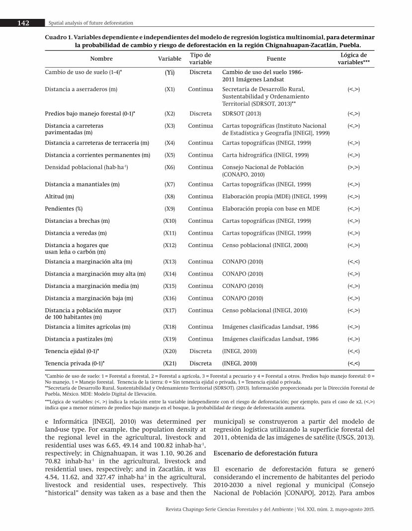
A total of 21 independent social, economic and environmental variables (Altamirano & Lara, 2010; Pineda et al., 2009; Pinedo, Pinedo, Quintana, & Martínez, 2007) correlated with the dependent variable, which are shown in Table 1, were considered. The values of the independent variables were calculated and extracted in a similar way to that used for the dependent variable. Subsequently, the database was purged by checking that each hectare or cell was represented by values of the dependent and independent variables through a visual inspection with the Microsoft Office Excel® software.

Baseline scenario for deforestation risk at regional and county levels With the independent and dependent variables, a multinomial logistic regression model was constructed (Hunter et al., 2003; Infante & Zarate, 2003; Montgomery, 2004). This type of model is a variant of the classic binary logistic model that relates the dependent variable with two or more explanatory or independent variables that are either qualitative or quantitative (Allison, 1999):

where:

Ŷi = Probability of a hectare of forest use changing use (where i = agricultural, livestock or residential uses)e = Base of natural logarithm = Intercept and estimators of the independent variables (xi )xi = Independent variables (x1, x2,…,x21)

The model was constructed using the stepwise procedure of the SAS 9.0 program (Statistical Analysis System, 2004) that lets you choose the subset of independent variables or regressors that should be considered in the model. This selection is made according to the order of importance or significance that helps explain the dependent variable (Beltrán, 2011; Silva, 1995). Finally,

entrenamiento y recorridos de campo, con apoyo del programa PCI GEOMATICS versión 9.1® (PCI GEOMATICS, 2004). Después se hizo un recorte regional y municipal de las imágenes utilizando el programa IDRISI Taiga mediante el modelo Image Calculator, para luego realizar un análisis bitemporal en el periodo 1986-2011 con el modelador de cambios CrossTab (Eastman, 2009) y obtener tres mapas de cambios de uso del suelo (uno regional y dos a nivel municipal). La superficie forestal estable y cambios ocurridos de uso forestal a usos agrícola, pecuario y residencial se obtuvieron en los tres mapas. Posteriormente, la información a nivel de hectárea se extrajo mediante una malla de 100 m x 100 m con el programa ArcGIS versión 9.3 (Environmental Systems Research Institute [ESRI], 2011) y con el modulo Create fishnet®. Finalmente, el centroide de cada polígono se obtuvo para elaborar una base de puntos y extraer sus valores con el comando extracción de valores de ráster a punto. La variable dependiente en el modelo tomó los siguientes valores: 1 = Forestal a forestal, 2 = Forestal a agrícola, 3 = Forestal a pecuario y 4 = Forestal a otros.

Estimación de las variables independientes

En total se consideraron 21 variables sociales, económicas y ambientales independientes (Altamirano & Lara, 2010; Pineda et al., 2009; Pinedo, Pinedo, Quintana, & Martínez, 2007) correlacionadas con la variable dependiente, las cuales se muestran en el Cuadro 1. Los valores de las variables independientes se calcularon y extrajeron de forma similar que la variable dependiente. Posteriormente, la base de datos se depuró revisando que cada hectárea o celda estuviera representada con valores de las variables dependiente e independientes a través de una inspección visual con el programa Microsoft Office Excel®.

Escenario base para riesgo de deforestación a nivel regional y municipal

Con las variables independientes y dependiente se construyó un modelo de regresión logística multinomial (Hunter et al., 2003; Infante & Zárate, 2003; Montgomery, 2004), el cual es una variante del modelo logístico binario clásico que relaciona la variable dependiente con dos o más variables explicativas o independientes ya sean cualitativas o cuantitativas (Allison, 1999):

donde: Ŷi = Probabilidad de que una hectárea de uso forestal cambie de uso (donde i = usos agrícola, pecuario o residencial)e = Base de logaritmo natural



the land-use change probability maps (regional and county) were built from the logistic regression model using the 2011 forest area, obtained from satellite imagery (USGS, 2013).

Future deforestation scenario

The future deforestation scenario was generated by considering the increase in inhabitants for the period 2010-2030 at the regional and county levels (Consejo Nacional de Población [CONAPO], 2012). For both levels, the average population density for the period 1985-2010 (Instituto Nacional de Estadística, Geografía

= Ordenada al origen y estimadores de las variables

independientes (xi )xi = Variables independientes (x1, x2,…,x21)

El modelo se construyó utilizando el procedimiento stepwise del programa SAS 9.0 (Statistical Analysis System, 2004) que permite elegir el subconjunto de variables independientes o regresoras que deben considerarse en el modelo. Esta selección se hace de acuerdo con el orden de importancia o significancia con que contribuyen a explicar la variable dependiente (Beltrán, 2011; Silva, 1995). Finalmente, los mapas de probabilidad de cambios de uso del suelo (regional y

Table 1. Dependent and independent variables of the multinomial logistic regression model to determine the probability of change and risk of deforestation in the Chignahuapan-Zacatlán region of Puebla.

Name Variable Type of variable

Source Logic of variables***

Land-use change (1-4)* (Yi) Discrete Land-use change, 1986-2011, based on Landsat images

Distance to sawmills (m) (X1) Continuous Secretaría de Desarrollo Rural, Sustentabilidad y Ordenamiento Territorial (SDRSOT, 2013)**

(<,>)

Properties under forest management (0-1)* (X2) Discrete SDRSOT (2013) (<,>)

Distance to paved roads (m) (X3) Continuous Topographic maps (Instituto Nacional de Estadística y Geografía [INEGI], 1999)

(<,>)

Distance to dirt roads (m) (X4) Continuous Topographic maps (INEGI, 1999) (<,>)

Distance to permanent watercourses (m) (X5) Continuous Hydrographic map (INEGI, 1999) (<,>)

Population density (inhab·ha-1) (X6) Continuous Consejo Nacional de Población (CONAPO, 2010)

(>,>)

Distance to springs (m) (X7) Continuous Topographic maps (INEGI, 1999) (<,>)

Elevation (m) (X8) Continuous Made by authors (DEM) (INEGI, 1999) (<,>)

Slopes (%) (X9) Continuous Made by authors based on DEM (<,>)

Distances to gaps (m) (X10) Continuous Topographic maps (INEGI, 1999) (<,>)

Distance to paths (m) (X11) Continuous Topographic maps (INEGI, 1999) (<,>)

Distance to homes that use firewood or charcoal (m)

(X12) Continuous Population census (INEGI, 2000) (<,>)

Distance to high-poverty areas (m) (X13) Continuous CONAPO (2010) (<,<)

Distance to extreme-poverty areas (m) (X14) Continuous CONAPO (2010) (<,>)

Distance to medium-poverty areas (m) (X15) Continuous CONAPO (2010) (<,>)

Distance to low-poverty areas (m) (X16) Continuous CONAPO (2010) (<,>)

Distance to a community with more than 100 inhabitants (m)

(X17) Continuous Population census (INEGI, 2010) (<,>)

Distance to agricultural limits (m) (X18) Continuous Classified Landsat images, 1986 (<,>)

Distance to pasture areas (m) (X19) Continuous Classified Landsat images, 1986 (<,>)

Ejidal ownership (0-1)* (X20) Discrete (INEGI, 2010) (<,<)

Private ownership (0-1)* (X21) Discrete (INEGI, 2010) (<,<)

*Change in land use: 1 = Forest to forest, 2 = Forest to agriculture, 3 = Forest to livestock and 4 = Forest to other uses. Properties under forest management: 0 = No management, 1 = Forest management. Land ownership: 0 = Without ejidal or private ownership, 1 = Ejidal or private ownership. **Secretaría de Desarrollo Rural, Sustentabilidad y Ordenamiento Territorial (SDRSOT). (2013). Information provided by the Dirección Forestal de Puebla, México. DEM: Digital Elevation Model.***Logic of variables: (<, >) indicates the relationship between the independent variable and the risk of deforestation; for example, in the case of x2, (<,>) indicates that the lower the number of properties under management in the forest, the greater the risk of deforestation.



e Informática [INEGI], 2010) was determined per land-use type. For example, the population density at the regional level in the agricultural, livestock and residential uses was 6.65, 49.14 and 100.82 inhab·ha-1, respectively; in Chignahuapan, it was 1.10, 90.26 and 70.82 inhab·ha-1 in the agricultural, livestock and residential uses, respectively; and in Zacatlán, it was 4.54, 11.62, and 327.47 inhab·ha-1 in the agricultural, livestock and residential uses, respectively. This “historical” density was taken as a base and then the

municipal) se construyeron a partir del modelo de regresión logística utilizando la superficie forestal del 2011, obtenida de las imágenes de satélite (USGS, 2013).

Escenario de deforestación futura

El escenario de deforestación futura se generó considerando el incremento de habitantes del periodo 2010-2030 a nivel regional y municipal (Consejo Nacional de Población [CONAPO], 2012). Para ambos

Cuadro 1. Variables dependiente e independientes del modelo de regresión logística multinomial, para determinar la probabilidad de cambio y riesgo de deforestación en la región Chignahuapan-Zacatlán, Puebla.

Nombre VariableTipo de variable

FuenteLógica de

variables***

Cambio de uso de suelo (1-4)* (Yi) Discreta Cambio de uso del suelo 1986-2011 Imágenes Landsat

Distancia a aserraderos (m) (X1) Continua Secretaría de Desarrollo Rural, Sustentabilidad y Ordenamiento Territorial (SDRSOT, 2013)**

(<,>)

Predios bajo manejo forestal (0-1)* (X2) Discreta SDRSOT (2013) (<,>)

Distancia a carreteraspavimentadas (m)

(X3) Continua Cartas topográficas (Instituto Nacional de Estadística y Geografía [INEGI], 1999)

(<,>)

Distancia a carreteras de terracería (m) (X4) Continua Cartas topográficas (INEGI, 1999) (<,>)

Distancia a corrientes permanentes (m) (X5) Continua Carta hidrográfica (INEGI, 1999) (<,>)

Densidad poblacional (hab·ha-1) (X6) Continua Consejo Nacional de Población (CONAPO, 2010)

(>,>)

Distancia a manantiales (m) (X7) Continua Cartas topográficas (INEGI, 1999) (<,>)

Altitud (m) (X8) Continua Elaboración propia (MDE) (INEGI, 1999) (<,>)

Pendientes (%) (X9) Continua Elaboración propia con base en MDE (<,>)

Distancias a brechas (m) (X10) Continua Cartas topográficas (INEGI, 1999) (<,>)

Distancia a veredas (m) (X11) Continua Cartas topográficas (INEGI, 1999) (<,>)

Distancia a hogares que usan leña o carbón (m)

(X12) Continua Censo poblacional (INEGI, 2000) (<,>)

Distancia a marginación alta (m) (X13) Continua CONAPO (2010) (<,<)

Distancia a marginación muy alta (m) (X14) Continua CONAPO (2010) (<,>)

Distancia a marginación media (m) (X15) Continua CONAPO (2010) (<,>)

Distancia a marginación baja (m) (X16) Continua CONAPO (2010) (<,>)

Distancia a población mayor de 100 habitantes (m)

(X17) Continua Censo poblacional (INEGI, 2010) (<,>)

Distancia a límites agrícolas (m) (X18) Continua Imágenes clasificadas Landsat, 1986 (<,>)

Distancia a pastizales (m) (X19) Continua Imágenes clasificadas Landsat, 1986 (<,>)

Tenencia ejidal (0-1)* (X20) Discreta (INEGI, 2010) (<,<)

Tenencia privada (0-1)* (X21) Discreta (INEGI, 2010) (<,<)

*Cambio de uso de suelo: 1 = Forestal a forestal, 2 = Forestal a agrícola, 3 = Forestal a pecuario y 4 = Forestal a otros. Predios bajo manejo forestal: 0 = No manejo, 1 = Manejo forestal. Tenencia de la tierra: 0 = Sin tenencia ejidal o privada, 1 = Tenencia ejidal o privada. **Secretaría de Desarrollo Rural, Sustentabilidad y Ordenamiento Territorial (SDRSOT). (2013). Información proporcionada por la Dirección Forestal de Puebla, México. MDE: Modelo Digital de Elevación.

***Lógica de variables: (<, >) indica la relación entre la variable independiente con el riesgo de deforestación; por ejemplo, para el caso de x2, (<,>) indica que a menor número de predios bajo manejo en el bosque, la probabilidad de riesgo de deforestación aumenta.



new inhabitants were “populated,” giving priority to those cells with the greatest likelihood of land-use change in the probability maps.

Comparison of scales

A comparative future analysis of the deforestation risk maps at the regional and county levels was performed qualitatively and quantitatively.

Results and discussion

Detection of land-use change (dependent variable)

Regional

The main land use in the Chignahuapan-Zacatlán region is agriculture, which increased by 7.9 % in the period from 1986 to 2011. This value is consistent with data reported by Franco, Regil, González, and Nava (2006) in a study conducted in Nevado de Toluca National Park, Mexico, during the period 1972-2000. In general, Evangelista et al. (2010) note that in the Sierra Norte de Puebla there is a trend towards increased agricultural and residential land use; the livestock area in 2011 decreased by 75 %, while agricultural and residential areas increased. For its part, forest use, second in importance, retained only 85 % of its land base due to losses caused by population growth and inordinate use of natural resources (SMRN, 2007).

County

Agricultural land is the most important in Chignahuapan county. Mahar and Schneider (1994) indicate that the advance of the agricultural frontier is one of the main causes of deforestation. On the other hand, forest use accounts for 53 % of the territory in Zacatlán. During the 25 years analyzed, livestock area decreased in both counties, while residential use increased. Despite the land-use changes, 57,693 ha of stable forest use were determined at the regional level, of which 29,654 ha (51.40 %) are in Chignahuapan and 28.039 ha (48.60 %) in Zacatlán.

Importance and significance of variables at the regional and county levels

The results of logistic regression and the significance of the variables that help explain the change in land use are shown in Tables 2, 3 and 4. At the regional level, the number of significant variables for land-use changes from forest to agriculture, forest to livestock and forest to residential were 17, 17 and 14, respectively (Table 2); for Chignahuapan, they were 14, 5 and 4 (Table 3); and for Zacatlán, they were 19, 13 and 11 (Table 4). The number of significant variables (17, 14 and 19) that predict land-use change from forest to agriculture is

niveles, la densidad poblacional promedio de 1985-2010 (Instituto Nacional de Estadística, Geografía e Informática [INEGI], 2010) se determinó por tipo de uso de suelo. Por ejemplo, la densidad poblacional a nivel región en los usos agrícola, pecuario y residencial fue de 6.65, 49.14 y 100.82 hab·ha-1, respectivamente; en Chignahuapan fue de 1.10, 90.26 y 70.82 hab·ha-1 en los usos agrícola, pecuario y residencial, respectivamente; y en Zacatlán fue de 4.54, 11.62, y 327.47 hab·ha-1 en los usos agrícola, pecuario y residencial, respectivamente. Esta densidad “histórica” se tomó como base y se procedió a “poblar”, los nuevos habitantes dando prioridad a aquellas celdas con mayor probabilidad de cambio de uso de suelo en los mapas de probabilidad.

Comparación de escalas

Un análisis comparativo futuro de los mapas de riesgo de deforestación a nivel regional y municipal se realizó cualitativa y cuantitativamente.

Resultados y discusión

Detección de cambio de uso del suelo (variable dependiente)

Regional

El uso principal de suelo en la región Chignahuapan-Zacatlán es el agrícola, el cual incrementó 7.9 % en el periodo de 1986 a 2011. Este valor concuerda con los datos reportados por Franco, Regil, González, y Nava (2006) en el estudio realizado en el Parque Nacional Nevado de Toluca, México, durante el periodo 1972-2000. En general, Evangelista et al. (2010) señalan que en la Sierra Norte de Puebla existe tendencia a incrementar los terrenos de uso agrícola y residencial; la superficie de la actividad pecuaria en 2011 disminuyó 75 %, mientras que las áreas agrícolas y residenciales incrementaron. Por su parte, el uso forestal, segundo en importancia, se conservó sólo en 85 % debido a las pérdidas ocasionadas por el incremento poblacional y al aprovechamiento desordenado de los recursos naturales (SMRN, 2007).

Municipal

La superficie agrícola es la más relevante en el municipio de Chignahuapan. Mahar y Schneider (1994) indican que el avance de la frontera agrícola es una de las principales causas de deforestación. Por otra parte, 53 % del territorio de Zacatlán es de uso forestal. Durante los 25 años analizados, la superficie pecuaria disminuyó en ambos municipios, mientras que el uso residencial aumentó. Pese a los cambios de uso del suelo, se determinaron 57,693 ha de uso forestal estable a nivel regional, de las cuales 29,654 ha (51.40 %) corresponden a Chignahuapan y 28,039 ha (48.60 %) a Zacatlán.



Table 2. Results of the logistic regression. Estimators of the independent variables, to determine the probability of change and risk of deforestation in the Chignahuapan-Zacatlán region of Puebla.

Cuadro 2. Resultados de la regresión logística. Estimadores de las variables independientes para determinar la probabilidad de cambio y riesgo de deforestación en la región Chignahuapan-Zacatlán, Puebla.

Variable = Forest-Agrícultural (1.3113)/ = Forestal-Agrícola (1.3113)

= Forest-Livestock (-2.1263)/ = Forestal-Pecuario (-2.1263)

= Forest-Residential (13.2483)/ Forestal-Residencial (13.2483)

Wald (Pr > 2 ) Pr > 2

Wald (Pr > 2 ) Wald (Pr > 2 )

(X1) 0.00001 0.0396 4.24 0.00006 0.0202 5.39 -0.00369 <.0001 72.27

(X2) -0.6253 <.0001 209.22 -0.477 0.0029 8.85 NS NS 0.08

(X3) NS NS 2.61 NS NS 0.99 0.00129 <.0001 16.25

(X4) NS NS 0.06 NS NS 0.14 0.00178 <.0001 19.25

(X5) NS NS 2.22 0.00026 <.0001 18.28 0.00383 <.0001 100.56

(X6) NS NS 3.16 1.8421 <.0001 38.21 5.3737 <.0001 16.28

(X7) -0.00002 0.0302 4.70 0.00014 0.0003 13.21 NS NS 3.64

(X8) -0.00071 <.0001 64.42 -0.0018 <.0001 100.46 -0.01470 <.0001 18.53

(X9) -0.04810 <.0001 1,699.11 -0.00363 0.0193 5.47 -0.19970 <.0001 66.28

(X10) -0.00006 <.0001 19.80 0.00020 <.0001 27.37 NS NS 1.69

(X11) -0.00048 <.0001 132.27 0.00022 0.0163 5.77 -0.00336 <.0001 21.75

(X12) -0.00016 <.0001 18.77 -0.00057 0.0003 12.94 NS NS 1.01

(X13) 0.00015 <.0001 17.55 0.00034 <.0001 18.30 0.00358 <.0001 48.60

(X14) -0.00007 <.0001 91.70 NS NS 1.86 NS NS 0.83

(X15) -0.00007 <.0001 58.84 -0.00006 0.0381 4.30 -0.00143 <.0001 26.28

(X16) -0.00002 <.0001 17.66 -0.00009 <.0001 16.60 NS NS 3.30

(X17) -0.00041 <.0001 134.60 NS NS 0.19 -0.00274 <.0001 17.67

(X18) -0.00287 <.0001 1,111.74 -0.00013 0.2044 1.61 -0.02420 <.0001 38.78

(X19) 0.00079 <.0001 135.58 -0.00241 <.0001 60.51 0.00136 0.0411 4.17

(X20) 2.0573 <.0001 303.60 -0.73350 0.0004 12.57 NS NS 0.00

(X21) 2.1117 <.0001 346.28 -1.1217 <.0001 69.99 7.34210 0.9429 0.01

(X1) Distance to sawmills, (X2) Properties under forest management, (X3) Distance to paved roads, (X4) Distance to dirt roads, (X5) Distance to permanent watercourses, (X6) Population density, (X7) Distance to springs, (X8) Elevation, (X9) Slopes, (X10) Distance to gaps, (X11) Distance to paths, (X12) Distance to homes that use firewood or charcoal. (X13) Distance to high-poverty areas, (X14) Distance to extreme-poverty areas, (X15) Distance to medium-poverty areas, (X16) Distance to low-poverty areas, (X17) Distance to a community with more than 100 inhabitants, (X18) Distance to agricultural limits, (X19) Distance to pasture areas, (X20) Ejidal ownership and (X21) Private ownership. Wald 2 : Wald test that has Chi-squared distribution. NS = Not significant (P ≤ 0.05)

(X1) Distancia a los aserraderos, (X2) Predios bajo manejo forestal, (X3) Distancia a carreteras pavimentadas, (X4) Distancia a carreteras de terracería, (X5) Distancia a corrientes permanentes, (X6) Densidad poblacional, (X7) Distancia a manantiales, (X8) Altitud, (X9) Pendientes, (X10) Distancia a brechas, (X11) Distancia a veredas, (X12) Distancia a hogares que usan leña o carbón, (X13) Distancia a marginación alta, (X14) Distancia a marginación muy alta, (X15) Distancia a marginación media, (X16) Distancia a marginación baja, (X17) Distancia a población mayor de 100 habitantes, (X18) Distancia a límites agrícolas, (X19) Distancia a pastizales, (X20) Tenencia ejidal y (X21) Tenencia privada. Wald 2 : Test de Wald que posee distribución Chi-cuadrada. NS = No significativa (P ≤ 0.05)

Pr > 2 Pr >2



Table 3. Results of the logistic regression. Estimators of the independent variables, to determine the probability of change and risk of deforestation in Chignahuapan county, Puebla.

Cuadro 3. Resultados de la regresión logística. Estimadores de las variables Independientes, para determinar la probabilidad de cambio y riesgo de deforestación en el municipio de Chignahuapan, Puebla.

Variable =

Forest / Agricultural (5.3736)*

= Forestal / Agrícola (5.3736)*

= Forest / Livestock (-3.7933)*

= Forestal / Pecuario (-3.7933)*

= Forest / Residential (23.3854)*/

= Forestal /Residencial (23.3854)*

Wald (Pr > 2 ) Wald (Pr > 2 ) Wald (Pr > 2 )

(X1) 0.00004 <.0001 18.00 NS 0.2884 1.18 NS 0.0582 3.56

(X2) -0.4791 <.0001 89.34 NS 0.6773 0.18 NS 0.4756 0.50

(X3) 0.00005 0.0003 14.05 -0.00061 0.0437 4.01 NS 0.7806 0.08

(X4) 0.00009 0.0003 13.94 NS 0.6126 0.24 NS 0.0814 3.05

(X5) -0.00006 0.0005 12.59 NS 0.7035 0.15 -0.00194 0.0024 9.11

(X6) NS NS NS NS NS NS NS NS NS

(X7) -0.00008 <.0001 35.53 NS 0.263 1.27 NS 0.1606 1.98

(X8) -0.00160 <.0001 79.49 NS 0.67030 0.21 NS 0.058 3.61

(X9) -0.05440 <.0001 703.79 NS 0.77980 0.07 -0.28490 0.0005 12.23

(X10) NS 0.4717 0.28 0.00128 0.00730 7.18 NS 0.2456 1.34


(X12) 0.00023 0.001 11.13 0.0038 0.04310 4.08 NS 0.8181 0.05

(X13) NS 0.9404 0.02 -0.0034 0.00410 8.26 0.00557 0.0308 4.67

(X14) -0.00005 0.0001 14.99 NS 0.70840 0.15 NS 0.1922 1.71


(X16) -0.0001 <.0001 54.59 NS 0.81010 0.06 NS 0.3182 0.99

(X17) -0.00046 <.0001 87.68 NS 0.16710 1.92 -0.00642 0.0325 4.57

(X18) -0.00397 <.0001 746.97 NS 0.46450 0.55 NS 0.0885 2.91

(X19) 0.00084 <.0001 113.37 0.00154 0.01640 5.80 NS 0.3769 0.79



(X1) Distance to sawmills, (X2) Properties under forest management, (X3) Distance to paved roads, (X4) Distance to dirt roads, (X5) Distance to permanent watercourses, (X6) Population density, (X7) Distance to springs, (X8) Elevation, (X9) Slopes, (X10) Distance to gaps, (X11) Distance to paths, (X12) Distance to homes that use firewood or charcoal, (X13) Distance to high-poverty areas, (X14) Distance to extreme-poverty areas, (X15) Distance to medium-poverty areas, (X16) Distance to low-poverty areas, (X17) Distance to a community with more than 100 inhabitants, (X18) Distance to agricultural limits, (X19) Distance to pasture areas, (X20) Ejidal ownership and (X21) Private ownership. Wald 2 : Wald test that has Chi-squared distribution. NS = Not significant (P ≤ 0.05). * Estimated value of the intercept.(X1) Distancia a los aserraderos, (X2) Predios bajo manejo forestal, (X3) Distancia a carreteras pavimentadas, (X4) Distancia a carreteras de terracería, (X5) Distancia a corrientes permanentes, (X6) Densidad poblacional, (X7) Distancia a manantiales, (X8) Altitud, (X9) Pendientes, (X10) Distancia a brechas, (X11) Distancia a veredas, (X12) Distancia a hogares que usan leña o carbón, (X13) Distancia a marginación alta, (X14) Distancia a marginación muy alta, (X15) Distancia a marginación media, (X16) Distancia a marginación baja, (X17) Distancia a población mayor de 100 habitantes, (X18) Distancia a límites agrícolas, (X19) Distancia a pastizales, (X20) Tenencia ejidal y (X21) Tenencia privada. Wald 2 :Test de Wald que posee distribución Chi-cuadrada. NS = No significativa (P ≤ 0.05). * Valor estimado de la ordenada al origen.

Pr > 2

similar at the regional and county level. This was not the case for land-use changes from forest to livestock and forest to residential in Chignahuapan, for which the number of variables are 5 and 4, respectively. In the same county there were five non-significant variables for the three land-use changes (Table 3). In the nine models obtained, the estimators of the 21 independent variables show either a positive or negative sign depending on the change of use in question and the scale analyzed. For example, at the regional level there is a positive correlation between the change in

Importancia y significancia de variables a nivel regional y municipal

Los resultados de la regresión logística y la significancia de las variables que contribuyen a explicar el cambio de uso de suelo se muestran en los Cuadros 2, 3 y 4. A nivel región, el número de variables significativas para los cambios de uso de suelo forestal a agrícola, forestal a pecuario y forestal a residencial fueron 17, 17 y 14, respectivamente (Cuadro 2); para Chignahuapan fueron 14, 5 y 4 (Cuadro 3); y para Zacatlán fueron 19, 13 y 11 (Cuadro 4). El número de variables significativas

Pr > 2Pr > 2



Table 4. Results of the logistic regression. Estimators of the independent variables, to determine the probability of change and risk of deforestation in Zacatlán county, Puebla.

Cuadro 4. Resultados de la regresión logística. Estimadores de las variables independientes para determinar la probabilidad de cambio y riesgo de deforestación en el municipio de Chignahuapan, Puebla.

Variable

= Forest /Agricultural (-1.3437) /

= Forestal /Agrícola (-1.3437)

= Forest / Livestock (-0.1598) / = Forestal / Pecuario (-0.1598)

= Forest /Residential (55.4306) / = Forestal /Residencial (55.4306)

Pr > 2Wald (Pr > 2 ) Pr > 2 Wald (Pr > 2 ) Pr > 2 Wald (Pr > 2 )

(X1) 0.00004 0.0366 4.37 0.00006 0.0453 4.01 -0.00856 <.0001 42.44

(X2) -0.80240 <.0001 131.32 -0.51440 0.006 7.56 NS 0.9402 0.01

(X3) 0.00005 0.0034 8.57 NS 0.0517 3.78 NS 0.2092 1.58

(X4) -0.00027 <.0001 50.89 NS 0.1164 2.46 NS 0.2598 1.27

(X5) 0.00022 <.0001 44.61 0.00042 <.0001 27.48 0.00387 <.0001 18.77

(X6) 1.08870 0.0032 8.68 NS 0.5798 0.31 -22.17910 0.0244 5.06

(X7) 0.00008 <.0001 18.36 NS 0.0525 3.76 NS 0.2474 1.34

(X8) NS 0.1030 2.66 -0.00229 <.0001 119.80 NS 0.0672 3.35

(X9) -0.0498 <.0001 960.99 -0.00411 0.0105 6.55 -0.1229 0.0004 12.52

(X10) -0.0001 <.0001 24.86 0.00009 0.0327 4.56 NS 0.0659 3.38

(X11) -0.00081 <.0001 151.02 NS 0.252 1.31 -0.00677 <.0001 18.47

(X12) -0.00032 <.0001 43.04 -0.00056 0.001 10.92 0.00582 0.0063 7.45

(X13) NS 0.8246 0.05 0.00020 0.0196 5.45 0.00318 0.0258 4.97

(X14) -0.0001 <.0001 61.81 NS 0.9674 0.00 NS 0.4854 0.49

(X15) -0.00005 <.0001 15.94 NS 0.0766 3.14 -0.00257 0.0087 6.89

(X16) -0.00004 <.0001 16.91 -0.00011 <.0001 15.61 NS 0.6108 0.26

(X17) -0.00022 0.0002 14.18 0.00046 0.0047 8.01 -0.00734 0.0001 14.82

(X18) -0.00209 <.0001 301.87 NS 0.1839 1.77 -0.01080 0.0364 4.38

(X19) 0.000637 <.0001 15.53 -0.00540 <.0001 158.11 0.01150 <.0001 20.97

(X20) 1.9632 <.0001 217.78 -0.72260 0.0042 8.19 NS 0.9584 0.00

(X21) 2.1138 <.0001 309.76 -0.99700 <.0001 50.75 NS 0.9824 0.00

(X1) Distance to sawmills, (X2) Properties under forest management, (X3) Distance to paved roads, (X4) Distance to dirt roads, (X5) Distance to permanent watercourses, (X6) Population density, (X7) Distance to springs, (X8) Elevation, (X9) Slopes, (X10) Distance to gaps, (X11) Distance to paths, (X12) Distance to homes that use firewood or charcoal, (X13) Distance to high-poverty areas, (X14) Distance to extreme-poverty areas, (X15) Distance to medium-poverty areas, (X16) Distance to low-poverty areas, (X17) Distance to a community with more than 100 inhabitants, (X18) Distance to agricultural limits, (X19) Distance to pasture areas, (X20) Ejidal ownership and (X21) Private ownership. Wald 2 : Wald test that has chi-square distribution. NS = Not significant (P ≤ 0.05)

(X1) Distancia a los aserraderos, (X2) Predios bajo manejo forestal, (X3) Distancia a carreteras pavimentadas, (X4) Distancia a carreteras de terracería, (X5) Distancia a corrientes permanentes, (X6) Densidad poblacional, (X7) Distancia a manantiales, (X8) Altitud, (X9) Pendientes, (X10) Distancia a brechas, (X11) Distancia a veredas, (X12) Distancia a los hogares que usan leña o carbón, (X13) Distancia a marginación alta, (X14) Distancia a marginación muy alta, (X15) Distancia a marginación media, (X16) Distancia a marginación baja, (X17) Distancia a población mayor de 100 habitantes, (X18) Distancia a límites agrícolas, (X19) Distancia a pastizales, (X20) Tenencia ejidal y (X21) Tenencia privada. Wald 2 :Test de Wald que posee distribución chi-cuadrada. NS = No significativa (P ≤ 0.05)

land use from forest to agriculture and the distance to sawmills (x1), distance to areas with high poverty (x13), distance to pasture areas (x19), ejidal (communal land) ownership (x20) and private ownership (x21). That is,

(17, 14 y 19) que predicen el cambio de uso de suelo de forestal a agrícola es similar a nivel región y municipio, no así para los usos de suelo de forestal a pecuario y de forestal a residencial en Chignahuapan, cuyo número



one hectare of land with forest use is more likely to be changed to agricultural use if the land is farther away from sawmills and pasture areas and if it is ejido or private land. For the same use and region, all other significant variables show negative correlation (Table 2). The interpretation of the signs is similar in other uses for the region and for the counties under study (Tables 2, 3 and 4).

All variables have different relative importance in each model at the regional and county levels (Table 5). At the regional level, and with a negative relationship, the variables minimum distance to agricultural areas (x18), elevation (x8) and slope (x9) are the ones that most influence deforestation (Tables 2 and 5). This contrasts with Chaves and Rosero-Bixby (2001), who indicate that the minimum distance to transportation routes has little influence on the deforestation process, and with Pineda et al. (2009), who agree that elevation and slope (> 20 %) are causes of deforestation. This is probably because the studies were performed with a different spatial scale. For example, at the county level, the behavior of the three aforementioned variables was different; for Chignahuapan, they were not significant, except for the change in land use from forest to agriculture (Table 3). Some variables such as the distance to: paved roads (x3), dirt roads (x4), permanent watercourses (x5) and communities with a population of more than 100 inhabitants (x17) helped explain deforestation in both counties; however, these variables were not significant at the regional level. In short, estimators of the independent variables at the regional and county levels generate a different model for each land-use change (forest-agriculture, forest-livestock and forest-residential) (Alcaraz et al, 2008; Bocco et al., 2001). This allows us to understand that the patterns of land-cover and land-use change vary widely from one region to one county and vice versa.

Model validation

In building the deforestation risk models, there was no correlation between independent variables. In addition, Table 6 shows that the models were not affected by multicollinearity, since they had tolerances of greater than 1 and variance inflation factors of less than 10. This suggests that there is no linear relationship between the model’s independent variables (Kutner, Nachtsheim, Neter, & Li, 2005). On average 80.7 % concordant observations were obtained at the regional and county levels, indicating that the independent and dependent variables are ordered in the same direction, thereby favoring the model’s predictive ability. A perfect positive association occurs when all pairs are concordant. All three models have R2

adj greater than 20 %; although the value is low, it is considered appropriate due to the inclusion of biophysical, economic and social variables. This situation has already been reported

de variables son 5 y 4, respectivamente. En este mismo municipio existieron cinco variables no significativas para los tres cambios de uso de suelo (Cuadro 3).

En los nueve modelos obtenidos, los estimadores de las 21 variables independientes muestran signo positivo o negativo dependiendo del cambio de uso que se trate y de la escala analizada. Por ejemplo, a nivel región existe correlación positiva entre el cambio de uso de suelo de forestal a agrícola y la distancia a aserraderos (x1), distancia a áreas con marginación alta (x13), distancia a pastizales (x19), tenencia ejidal (x20) y tenencia privada (x21). Es decir, una hectárea de terreno con uso forestal tiene probabilidad mayor de ser cambiada a uso agrícola, si el terreno está más alejado de los aserraderos y de los pastizales y si es terreno ejidal o privado. Para el mismo uso y región, el resto de las variables significativas presentan correlación negativa (Cuadro 2). La interpretación de los signos es similar en los otros usos para la región y para los municipios bajo estudio (Cuadros 2, 3 y 4).

Todas las variables presentan importancia relativa diferente en cada modelo a nivel regional y municipal (Cuadro 5). A nivel regional, y con una relación negativa, las variables distancia mínima a zonas agrícolas (x18), altitud (x8) y pendiente (x9) son las que más influyen en la deforestación (Cuadros 2 y 5). Esto contrasta con Chaves y Rosero-Bixby (2001), quienes indican que la distancia mínima a vías de comunicación influye poco en el proceso de deforestación, y con Pineda et al. (2009), quienes concuerdan en que la altitud y la pendiente (> 20 %) son causas de deforestación. Lo anterior probablemente se debe a que los estudios se realizaron con una escala espacial diferente. Por ejemplo, a nivel municipal, el comportamiento de las tres variables mencionadas fue distinto; para Chignahuapan no fueron significativas, excepto para el cambio de uso de suelo de forestal a agrícola (Cuadro 3). Algunas variables como la distancia a: carreteras pavimentadas (x3), terracerías (x4), corrientes permanentes (x5) y poblados con densidad mayor de 100 habitantes (x17) contribuyeron a explicar la deforestación en ambos municipios; sin embargo, estas variables no fueron significativas a nivel de región. En suma, los estimadores de las variables independientes a nivel regional y municipal generan un modelo diferente para cada cambio de uso de la tierra (forestal-agrícola, forestal-pecuario y forestal-residencial) (Alcaraz et al., 2008; Bocco et al., 2001). Lo anterior permite comprender que los patrones de cambio de cobertura y uso del suelo varían ampliamente de una región a municipio y viceversa.

Validación del modelo

En la construcción de los modelos de riesgo de deforestación no existió correlación entre variables independientes. Además, en el Cuadro 6 se observa que



Table 5. Order of importance of the independent variables and significance at scalar level, which help explain the risk of regional and county deforestation.

Cuadro 5. Orden de importancia de las variables independientes y significancia a nivel escalar, que contribuyen a explicar el riesgo de deforestación regional y municipal.

Variable

Region Chignahuapan Zacatlán

Wald (Pr > 2 ) Pr > 2

Importance*Importancia

Wald (Pr > 2 ) Pr > 2 Importance* Wald (Pr > 2 ) Pr > 2 Importance*

(X1) 118.87 < .0001 14 2,329.59 <.0001 11 189.76 <.0001 8

(X2) 584.75 < .0001 4 47.50 <.0001 6 589.12 <.0001 4

(X3) 20.29 <.0001 21 23.52 <.0001 10 13.68 0.0034 21

(X4) 25.09 < .0001 19 17.70 0.0005 15 36.99 <.0001 16

(X5) 225.17 < .0001 7 16.34 0.001 5 93.24 <.0001 13

(X6) 67.15 < .0001 18 NS NS NS 13.95 0.003 20

(X7) 22.05 < .0001 20 9.72 0.0211 8 38.84 <.0001 17

(X8) 2,551.55 < .0001 2 9.82 0.0201 1 1,139.77 <.0001 2

(X9) 1,975.69 < .0001 3 16.94 0.0007 2 1,895.10 <.0001 1

(X10) 60.49 < .0001 17 1,475.93 <.0001 13 32.43 <.0001 18

(X11) 157.76 < .0001 10 NS NS NS 181.53 <.0001 10

(X12) 325.28 < .0001 6 940.11 <.0001 14 362.59 <.0001 5

(X13) 118.39 < .0001 12 170.61 <.0001 12 108.81 <.0001 12

(X14) 162.81 < .0001 11 162.47 <.0001 16 134.38 <.0001 11

(X15) 70.65 < .0001 16 166.59 <.0001 9 15.78 0.0013 19

(X16) 76.31 < .0001 15 NS NS NS 54.48 <.0001 14

(X17) 124.64 < .0001 13 95.01 <.0001 7 46.55 <.0001 15

(X18) 3,600.43 < .0001 1 56.00 <.0001 3 1,013.95 <.0001 3

(X19) 399.22 < .0001 5 26.03 <.0001 4 197.00 <.0001 9

(X20) 404.19 < .0001 9 NS NS NS 261.09 <.0001 7

(X21) 207.78 < .0001 8 NS NS NS 331.65 <.0001 6

(X1) Distance to sawmills, (X2) Properties under forest management, (X3) Distance to paved roads, (X4) Distance to dirt roads, (X5) Distance to permanent watercourses, (X6) Population density, (X7) Distance to springs, (X8) Elevation, (X9) Slopes, (X10) Distance to gaps, (X11) Distance to paths, (X12) Distance to homes that use firewood or charcoal, (X13) Distance to high-poverty areas, (X14) Distance to extreme-poverty areas, (X15) Distance to medium-poverty areas, (X16) Distance to low-poverty areas, (X17) Distance to a community with more than 100 inhabitants, (X18) Distance to agricultural limits, (X19) Distance to pasture areas, (X20) Ejidal ownership and (X21) Private ownership. Wald 2 : Wald test that has chi-square distribution. NS = Not significant (P ≤ 0.05). *Importance: 1 more important in the deforestation process and 21 less important.(X1) Distancia a aserraderos, (X2) Predios bajo manejo forestal, (X3) Distancia a carreteras pavimentadas, (X4) Distancia a carreteras de terracería, (X5) Distancia a corrientes permanentes, (X6) Densidad poblacional, (X7) Distancia a manantiales, (X8) Altitud, (X9) Pendientes, (X10) Distancia a brechas, (X11) Distancia a veredas, (X12) Distancia a hogares que usan leña o carbón, (X13) Distancia a marginación alta, (X14) Distancia a marginación muy alta, (X15) Distancia a marginación media, (X16) Distancia a marginación baja, (X17) Distancia a población mayor de 100 habitantes, (X18) Distancia a límites agrícolas, (X19) Distancia a pastizales, (X20) Tenencia ejidal y (X21) Tenencia privada. Wald 2 : Test de Wald que posee distribución chi-cuadrada. NS = No significativa (P ≤ 0.05). *Importancia: 1 más importante en el proceso de deforestación y 21 menos importante.

in previous research (Gomben et al., 2012; Frías-Armenta, López-Escobar, & Díaz-Méndez, 2003; Hunter et al., 2003); therefore, the models were considered appropriate to predict the phenomenon of interest.

Estimating the probability of spatial deforestation in two scales

Regional: Forest-agriculture

Figure 1a shows the probability of one hectare of forest use changing to agricultural use, which is 45-90 %.

los modelos no fueron afectados por la multicolinealidad, ya que presentaron tolerancias mayores de uno y los factores de inflación de la varianza fueron menores de diez. Esto sugiere que no existe relación lineal entre las variables independientes del modelo (Kutner, Nachtsheim, Neter, & Li, 2005). En promedio se obtuvo 80.7 % de observaciones concordantes a nivel regional y municipal, lo que indica que las variables dependiente e independiente están ordenadas en la misma dirección favoreciendo la predicción del modelo. Una asociación positiva perfecta ocurre cuando todos los pares son concordantes. Los tres modelos poseen



Tables 2 and 5 indicate that the variables elevation and distance to agricultural limits are the most influential in the process. This is consistent with Mahar and Schneider (1994), who concur that the advance of the agricultural frontier increases the likelihood of deforestation.

Regional: Forest-livestock

The probability that one hectare changes from forest to livestock use varies from 10-50 %. This is related to 17 significant variables in the deforestation process due to livestock use (Table 2). The most important variables at the regional level were elevation and distance to pasture areas with a negative relationship (Table 2), indicating that forest land with lower elevation and less distance to pasture areas has a greater probability of deforestation. Figure 1b shows that this phenomenon occurs mainly in the cloud forest in the region’s northwest area (SMRN, 2007).

Regional: Forest-residential

Figure 1c plots the probability of land-use change. Table 2 shows the 14 variables that have an impact on the deforestation process. The trend towards changing

Figure 1. Probability of land-use change a) forest to agriculture, b) forest to livestock and c) forest to residential, through the Chignahuapan-Zacatlán regional model.

Figura 1. Probabilidad de cambio de uso de suelo: a) forestal a agrícola, b) forestal a pecuario y c) forestal a residencial, mediante el modelo regional Chignahuapan-Zacatlán.

R2adj mayor de 20 %; aunque el valor es bajo se considera

adecuado por la inclusión de variables biofísicas, económicas y sociales. Esta situación ya se ha reportado en investigaciones previas (Gomben et al., 2012; Frías-Armenta, López-Escobar, & Díaz-Méndez, 2003; Hunter et al., 2003), por tanto, los modelos se consideraron adecuados para predecir el fenómeno de interés.

Estimación de la probabilidad de deforestación espacial en dos escalas

Regional: Forestal-agrícola

La Figura 1a muestra la probabilidad de que una hectárea de uso forestal cambie a uso agrícola, la cual es de 45 a 90 %. Los Cuadros 2 y 5 indican que las variables altitud y distancia a límites agrícolas son las de mayor influencia en el proceso. Esto concuerda con Mahar y Schneider (1994), quienes corroboraron que el avance de la frontera agrícola incrementa la probabilidad de deforestación.

Regional: Forestal-pecuario

La probabilidad de que una hectárea cambie de uso forestal a pecuario varía de 10 a 50 %. Lo anterior se

Table 6. Measures of association of predicted probabilities and observed responses by the regional and county models.

Cuadro 6. Medidas de asociación de probabilidades predichas y respuestas observadas mediante el modelo regional y municipal.

Scale /Escala

Measures of association /Medidas de asociación

Pairs /Pares

Correlation indices /Índices de correlación

R2adj

(%)Multicollinearity / Multicolinealidad

Concordant /Concordante

(%)

Discordant /Discordante

(%)

Bound/ Ligado

(%)

Somers’D

Gamma Tau-a cTolerance /Tolerancia

VIF /FIV

Region 80.00 19.20 0.90 340,628,933 0.60 0.61 0.15 0.80 25.44 0.75 1.34

Chignahuapan 85.90 13.20 0.90 75,418,437 0.72 0.73 0.16 0.86 37.33 0.63 1.60

Zacatlán 76.30 22.90 0.80 94,900,581 0.53 0.53 0.15 0.76 20.12 0.80 1.25

VIF = Variance inflation factor. / FIV = Factor de inflación de la varianza.

a) b) c)

Symbols agricultural /Simbología agrícola

Symbols livestock /Simbología pecuaria

Symbols residential /Simbología residencial

0 - 033

0.33 -0.66

0.66 - 1

0 - 033

0.33 -0.66

0.66 - 1

0 - 033

0.33 -0.66

0.66 - 1

2210

000

2195

000

2180

000

2210

000

2195

000

2180

000

2210

000

2195

000

2180

000

2210

000

2195

000

2180

000

2210

000

2195

000

2180

000

2210

000

2195

000

2180

000

620000600000580000620000600000580000620000600000580000

620000600000580000 620000600000580000 620000600000580000

N N N



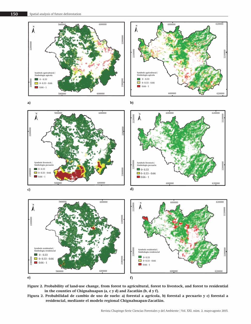
Figure 2. Probability of land-use change, from forest to agrícultural, forest to livestock, and forest to residential in the counties of Chignahuapan (a, c y d) and Zacatlán (b, d y f).

Figura 2. Probabilidad de cambio de uso de suelo: a) forestal a agrícola, b) forestal a pecuario y c) forestal a residencial, mediante el modelo regional Chignahuapan-Zacatlán.

a) b)

c)

f)

Symbols agricultural /Simbología agícola

0 - 0.33

0- 0.33 - 0.66

0.66 - 1

580000

580000

600000

600000

2200

000

2180

000

2180

000

2200

000

N

Symbols agricultural /Simbología agícola

0 - 0.33

0- 0.33 - 0.66

0.66 - 1

600000

600000 620000

620000

2210

000

2210

000

N

Symbols livestock /Simbología pecuario

0- 0.330- 0.33 - 0.660.66 - 1

600000

600000

620000

620000

2220

000

2220

000

2200

000

2200

000

N

Symbols livestock /Simbología pecuario

0- 0.33

0- 0.33 - 0.66

0.66 - 1

500000

500000

600000

600000

2200

000

2180

000

2200

000

2180

000

N

e)


0 - 0.330- 0.33 - 0.660.66 - 1

580000

580000

600000

600000

2200

000

2180

000

2200

000

2180

000

N


0- 0.330- 0.33 - 0.66

0.66 - 1

600000

600000

620000

620000

2220

000

2200

000

2220

000

2200

000

N

d)



relaciona con 17 variables significativas en el proceso de deforestación por uso pecuario (Cuadro 2). Las variables con mayor importancia relativa a nivel región fueron la altitud y la distancia a pastizales con una relación negativa (Cuadro 2), indicando que en los terrenos forestales con menor altitud y menor distancia a áreas con pastizales, la probabilidad de deforestación es mayor. En la Figura 1b se observa que dicho fenómeno se presenta principalmente en el bosque mesófilo de montaña al noroeste de la región (SMRN, 2007).

Regional: Forestal-residencial

La Figura 1c grafica la probabilidad de cambio de uso de suelo. El Cuadro 2 muestra las 14 variables que influyen en el proceso de deforestación. La tendencia de cambio a uso residencial es limitada pues las zonas forestales están alejadas de los centros urbanos y éstos se hallan rodeados de zonas agrícolas, teniendo mayor tendencia de cambio de agrícola a forestal (Pineda et al., 2009) y de residencial a uso agrícola.

Municipal: Forestal-agrícola

La probabilidad de que una hectárea de uso forestal cambie a uso agrícola (Figuras 2a, 2b) es superior de 60 %. En Chignahuapan y Zacatlán, la distancia a marginación alta no fue significativa (Cuadros 3 y 4) para determinar la probabilidad de cambio de uso forestal a uso agrícola, pese a que la agricultura es la principal actividad de ambos municipios y la principal promotora de la deforestación en México (Deininger & Minten, 1999).

Municipal: Forestal-pecuario

La probabilidad de cambio de uso forestal a pecuario (Figura 2c) está en función de las variables significativas para cada modelo; por ejemplo, para Chignahuapan se consideraron cinco variables significativas con probabilidades superiores de 95 % de cambiar una pequeña superficie forestal a uso pecuario (Cuadro 3). Por otra parte, para el municipio de Zacatlán se consideraron 13 variables significativas (Cuadro 4) para determinar la probabilidad de cambio (Figura 2d). En ese sentido, Rojas-López, González-Guillén, Gómez-Guerrero, y Romo-Lozano (2012) obtuvieron una probabilidad de 1 % para el cambio de uso forestal a pecuario; estas diferencias significativas probablemente se deben a la metodología empleada para el cálculo.

Municipal: Forestal-residencial

La probabilidad de cambio de uso forestal a uso residencial (Figuras 2e, 2f) es superior de 50 %. En ambos municipios, las variables significativas fueron distancia a corrientes permanentes, pendientes,

to residential use is limited because the forest areas are far from urban centers and surrounded by agricultural areas, having a greater tendency to change from agricultural to forest (Pineda et al., 2009) and from residential to agricultural use.

County: Forest-agriculture

The probability of one hectare of forest use changing to agricultural use (Figures 2a, 2b) is greater than 60 %. In Chignahuapan and Zacatlán, the distance to high-poverty areas was not significant (Tables 3 and 4) in determining the probability of change from forest to agricultural use, although agriculture is the main activity of both counties and the main driving force behind deforestation in Mexico (Deininger & Minten, 1999).

County: Forest-livestock

The probability of change from forest to livestock use (Figure 2c) is a function of the significant variables for each model; for example, for Chignahuapan, five significant variables with probabilities of more than 95 % to change a small forest area to livestock use were considered (Table 3). On the other hand, for Zacatlán county, 13 significant variables (Table 4) were considered to determine the probability of change (Figure 2d). In this regard, Rojas-López, González-Guillén, Gómez-Guerrero, and Romo-Lozano (2012) obtained a probability of 1 % for the change from forest to livestock use; these significant differences are probably due to the methodology used for the calculation.

County: Forest-residential.

The probability of forest use changing to residential use (Figures 2e, 2f) is greater than 50 %. In both counties, the significant variables were distance to permanent watercourses, slopes, high-poverty areas and a community of more than 100 inhabitants. The slope variable was significant with a negative sign, indicating that areas with gentle slopes are at increased risk of deforestation, while the variables permanent watercourses and a population of more than 100 inhabitants are considered indicators for establishing urban areas.

Scalar comparison of the risk of future deforestation

Figure 3 shows a qualitative comparison of the deforestation risk in Zacatlán and Chignahuapan. The regional model estimated a smaller area (2,308.2 ha) at risk of deforestation than the county-level models; however, this area is located in a different space, since the variables and estimators that determine this risk are different for each level. However, the risk of



deforestation in both scales occurs mainly in the forest-agriculture frontier (Mahar & Schneider, 1994).

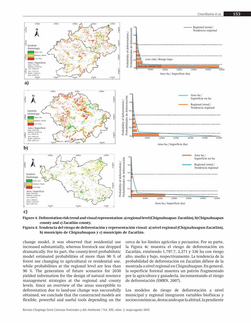
Figure 4 quantitatively compares the deforestation risk trend at the regional and county levels; it shows that the risk decreases as the area increases. At the regional level, an estimated 13,063 ha will be required to accommodate new inhabitants in 2030. Of these, 1,774.2 ha (13.6 %) are considered at high risk, 5,790.0 ha (44.3 %) at medium risk, and 5,499.6 (42.1 %) at low risk of deforestation (Figure 4a). The Chignahuapan model shows the same deforestation trend as the regional model; of the total area (29,654 ha), 7 % (2,097 ha) is at high risk, 14 % (4,395 ha) at medium risk and 15 % (2,097.2 ha) at low risk of deforestation (Figure 4b). These areas are located near agricultural and livestock limits. For its part, Figure 4c shows the deforestation risk in Zacatlán, with 1,797.7, 2,271 and 336 ha being at high, medium and low risk, respectively. The deforestation probability trend in Zacatlán differs from that shown at the regional level in Chignahuapan. Overall, the forest area shows a pattern fragmented by agriculture and livestock, increasing the risk of deforestation (SMRN, 2007).

Deforestation risk models at the county and regional levels integrated biophysical and socio-economic variables, highlighting that elevation, slope and distances to agricultural and livestock areas have a greater influence on land-use change and deforestation risk; however, distance to permanent watercourses is the most influential variable. Finally, Saab (1999) and Cueto (2006) agree that scale is a very important factor in delineating plans and strategies, so the selection of the scale to use depends on the objectives and characteristics of the study (García, Teich, & Balzarini, 2011); models built at one spatial scale and applied to another would generate biased interpretations. For example, if the regional model of land-use changes were applied to make estimates at the county level, an “ecological fallacy” would be generated, whereas if the county model were applied at the regional level, an “individualistic fallacy” would be committed. On the other hand, if the model generated for Chignahuapan county were applied to Zacatlán county or vice versa, a “cross fallacy or irregularity” would be committed (Brenner, 2001). Therefore, each scale must be appropriate to the phenomenon or process under study and must be used at the spatial level at which the policies and strategies for natural resource management, conservation and use are designed and applied. Conclusions

Through identifying patterns that govern land-use changes and deforestation risk, probabilistic models were constructed and applied for the region and the counties of Chignahuapan-Zacatlán, Puebla. Considering both study levels and the land-use

marginación alta y población mayor de 100 habitantes. La variable pendiente fue significativa con signo negativo, indicando que las áreas con pendientes poco pronunciadas tienen mayor riesgo de deforestación, mientras que las variables distancia a corrientes permanentes y a población mayor de 100 habitantes se consideran indicadores para establecer áreas urbanas.

Comparación escalar del riesgo de deforestación futura

La Figura 3 presenta una comparación cualitativa sobre el riesgo de deforestación en Chignahuapan y Zacatlán. El modelo regional estimó una menor superficie (2,308.2 ha) con riesgo de deforestación que los modelos a nivel municipal; sin embargo, esta superficie se localiza en diferente espacio, ya que las variables y estimadores que determinan tal riesgo son distintas para cada nivel. No obstante, el riesgo de deforestación en ambas escalas se presenta principalmente en la frontera forestal-agrícola (Mahar & Schneider, 1994).

La Figura 4 compara cuantitativamente la tendencia del riesgo de deforestación a nivel regional y municipal; se observa que el riesgo disminuye conforme la superficie incrementa. A nivel regional se estimaron 13,063 ha que serán requeridas para acomodar a los nuevos habitantes en el 2030. De ellas, 1,774.2 ha (13.6 %) se consideran con riesgo alto; 5,790.0 ha (44.3 %) con riesgo medio; y 5,499.6 (42.1 %) con riesgo bajo de deforestación (Figura 4a). El modelo de Chignahuapan muestra la misma tendencia de deforestación que el modelo regional; de la superficie total (29,654 ha), 7 % (2,097 ha) presenta riesgo alto, 14 % (4,395 ha) muestra riesgo medio y 15 % (2,097.2 ha) presenta riesgo bajo de deforestación (Figura 4b). Estas áreas se localizan

Figure 3. Qualitative comparison of scales concerning deforestation risk in Chignahuapan-Zacatlán, Puebla (regional and county levels).

Figura 3. Comparación cualitativa de escalas sobre riesgo de deforestación en Chignahuapan-Zacatlán, Puebla (nivel regional y municipal)

575000 587500 600000 612500 625000

575000 587500 600000 6125000 625000

2180

0022

0000

2220

000

2180

0022

0000

2220

000

Simbologia / Symbols

County scale / Escala municipal

Regional scale / Escala regional

Area / Superficie

Municipal: 15,372 ha / County: 15,372 haRegional: 13,063.8 ha / Regional: 13,063.8 ha



Figure 4. Deforestation risk trend and visual representation: a) regional level (Chignahuapan- Zacatlán), b) Chignahuapan county and c) Zacatlán county.

Figura 4. Tendencia del riesgo de deforestación y representación visual: a) nivel regional (Chignahuapan-Zacatlán), b) municipio de Chignahuapan y c) municipio de Zacatlán.

cerca de los límites agrícolas y pecuarios. Por su parte, la Figura 4c muestra el riesgo de deforestación en Zacatlán, existiendo 1,797.7, 2,271 y 336 ha con riesgo alto, medio y bajo, respectivamente. La tendencia de la probabilidad de deforestación en Zacatlán difiere de la mostrada a nivel regional en Chignahuapan. En general, la superficie forestal muestra un patrón fragmentado por la agricultura y ganadería, incrementando el riesgo de deforestación (SMRN, 2007).

Los modelos de riesgo de deforestación a nivel municipal y regional integraron variables biofísicas y socioeconómicas, destacando que la altitud, la pendiente

change model, it was observed that residential use increased substantially, whereas livestock use dropped dramatically. For its part, the county-level probabilistic model estimated probabilities of more than 90 % of forest use changing to agricultural or residential use, while probabilities at the regional level are less than 90 %. The generation of future scenarios for 2030 yielded information for the design of natural resource management strategies at the regional and county levels. Since an overview of the areas susceptible to deforestation due to land-use change was successfully obtained, we conclude that the constructed models are flexible, powerful and useful tools depending on the

SymbolsSimbología

High / Alto

Medium / Medio

Low / Bajo

Area / SuperficieHigh: 2,097.0 haMedium: 4,395.0 haLow: 2,097.6 ha

Alto: 2,097.0 haMedio: 4,395.0 haBajo: 2,097.2 ha

SymbolsSimbología

High / Alto

Medium / Medio

Low / Bajo



High / Alto

Medium / Medio

Low / Bajo



SymbolsSimbología

a)

b)

c)

565000 578000 591000 604000 617000

565000 578000 591000 604000 617000

578000 591000 604000

578000 591000 604000

591000 504000 617000

591000 504000 617000

2216

000

2204

000

2192

000

2180

000

2216

000

2204

000

2192

000

2180

000

2204

000

2192

000

2180

000

2204

000

2192

000

2180

000

2216

000

2204

000

2216

000

2204

000

Prob

abil

ity

of d

efor

esta

tion

/Pr

obab

ilid

ades

de

defo

rest

ació

n

Prob

abil

ity

of d

efor

esta

tion

/Pr

obab

ilid

ades

de

defo

rest

ació

n

Prob

abil

ity

of d

efor

esta

tion

/Pr

obab

ilid

ades

de

defo

rest

ació

n

Area ha / Superficie (ha)



Regional trend /Tendencia regional

Low risk / Riesgo bajo

Zero risk / Riesgo nulo00

1.0

0.8

0.6

0.4

0.2

10.000 20.000 30.000 40.000 50.000 60.000


Area ha /Superficie en ha

00

1.0

0.8

0.6

0.4

0.2

10.000 20.000 30.000 40.000 50.000 60.000

10.000 20.000 30.000 40.000 50.000 60.000


Area ha /Superficie en ha

00

1.0

0.8

0.6

0.4

0.2

0

0

0



y los límites a zonas agrícolas y pecuarias tienen mayor influencia en el cambio de uso del suelo y riesgo de deforestación; aunque, para el cambio de uso forestal a residencial, la distancia a corrientes permanentes es la variable que más influye. Finalmente, Saab (1999) y Cueto (2006) concuerdan que la escala es un factor muy importante en la delineación de planes y estrategias, por lo que la selección de la escala a utilizar depende de los objetivos y características del estudio (García, Teich, & Balzarini, 2011); los modelos construidos a una escala espacial y aplicados a otra, generaría interpretaciones sesgadas. Por ejemplo, si se quisiera aplicar el modelo regional de cambios de uso de suelo, para hacer estimaciones a nivel municipal se generaría una “falacia ecológica”, contrariamente se cometería la “falacia individualista”. Por otra parte, si se quisiera aplicar el modelo generado para el municipio de Chignahuapan y aplicarlo al municipio de Zacatlán o viceversa se cometería la “falacia o irregularidad transversal” (Brenner, 2001). Por tanto, cada escala debe ser apropiada al fenómeno o proceso bajo estudio y debe utilizarse al nivel espacial al cual se diseñen y apliquen las políticas y estrategias de manejo, conservación y aprovechamiento de los recursos naturales.

Conclusiones

A través de la identificación de patrones que rigen los cambios de uso del suelo y riesgo de deforestación, se construyeron y aplicaron modelos probabilísticos para la región y los municipios de Chignahuapan-Zacatlán, Puebla. Considerando ambos niveles de estudio y el modelo de cambio de uso de suelo, se observó que el uso residencial incrementó sustancialmente; sin embargo, se identificó que el uso pecuario disminuyó drásticamente. Por su parte, el modelo probabilístico a nivel municipal estimó probabilidades mayores de 90 % de cambios de uso forestal a uso agrícola o residencial, mientras que a nivel regional existen probabilidades menores de 90 %. La generación de escenarios futuros para el 2030 permitió obtener información para el diseño de estrategias de manejo sobre los recursos naturales a nivel regional y municipal. Debido a que se obtuvo un panorama de las áreas susceptibles a la deforestación por cambio de uso, se considera que los modelos construidos son herramientas flexibles, poderosas y útiles dependiendo de la escala a la cual se deseen generar estrategias de uso de los recursos naturales.

Agradecimientos

A la Línea Prioritaria de Investigación 1 (LPI1): Manejo Sustentable de los Recursos Naturales del Colegio de Postgraduados por el financiamiento.

scale at which one wishes to generate strategies for use of natural resources.

Acknowledgments

The authors are grateful to the Colegio de Postgraduados for providing funding for this study under Priority Research Line 1 (known by the Spanish acronym LPI1): Sustainable Management of Natural Resources.

References / Referencias

Alcaraz, S. D., Baldi, P. G., & Garbulsky, M. F. (2008). Análisis de la dinámica temporal del NDVI en áreas protegidas: Tres casos de estudio a distintas escalas espaciales, temporales y de gestión. Ecosistemas, 17, 108–117. Obtenido de http://www.redalyc.org/articulo.oa?id=54017106010

Allison, P. D. (1999). Logistic regression using the SAS system: Theory and application. Cary, NC, USA: John Wiley & Sons-SAS Institute Inc.

Altamirano, A., & Lara, A. (2010). Deforestación en ecosistemas templados de la precordillera andina del centro-sur de Chile. Bosque, 31, 53–64. doi: 10.4067/S0717-92002010000100007

Beltrán, C. (2011). Aplicación del análisis de regresión logística multinomial en la clasificación de textos académicos: Biometría, filosofía y lingüística informática. INFOSUR, 5, 53–64. Obtenido de http://www.infosurrevista.com.ar/biblioteca/INFOSUR-Nro5-2011-Beltran.pdf

Bocco, G., Mendoza, M., & Masera, O. R. (2001). La dinámica del cambio del uso del suelo en Michoacán: Una propuesta metodológica para el estudio de los procesos de deforestación. Investigaciones Geográficas, 44, 18–36. Obtenido de http://www.oikos.unam.mx/Bioenergia/images/PDF/CC/CC-Bosques/la_dinamica_del_cambio_del_uso_del_suelo.pdf

Brenner, N. (2001). The limits to scale? Methodological reflections on scalar structuration. Progress in Human Geography, 25, 591–610. doi: 10.1191/030913201682688959

Chaves, E. E., & Rosero-Bixby, L. (2001). Valoración del riesgo de deforestación futura en Costa Rica. Uniciencia, 18, 29–38. Obtenido de http://ccp.ucr.ac.cr/bvp/pdf/bosques/chaves.pdf

Consejo Nacional de Población (CONAPO). (2012). Índice de marginación por localidad 2010. México, D. F.: Autor.

Cueto, V. R. (2006). Escalas en ecología: Su importancia para el estudio de la selección de hábitat en aves. Hornero, 21, 1–13. Obtenido de http://www.scielo.org.ar/pdf/hornero/v21n1/v21n1a01.pdf

Deininger, K. W., & Minten, B. (1999). Poverty, policies, and deforestation: The case of Mexico. Economic Development and Cultural Change, 47, 313–344. Obtenido de http://www.jstor.org/stable/10.1086/452403

End of English version

Fin de la versión en Español



Eastman, R. J. (2009). IDRISI Taiga Guide to GIS and image processing. Worcester, MA, USA: Clark Labs.

Environmental Systems Research Institute (ESRI). (2011). Software ArcGIS, versión 10.0. Redlands, CA, USA: Autor.

Evangelista, O. V., López, B. J., Caballero, N. J., & Martínez, A. M. A. (2010). Patrones espaciales de cambio de cobertura y uso del suelo en el área cafetalera de la Sierra Norte de Puebla. Investigaciones Geográficas, 72, 23–38. Obtenido de http://www.revistas.unam.mx/index.php/rig/article/view/19273

Franco, M., S., Regil, G. H. H., González, E. C., & Nava, B. G. (2006). Cambio de uso del suelo en el Parque Nacional Nevado de Toluca, México, en el periodo 1972-2000. Investigaciones Geográficas, 61, 38–57. Obtenido de http://www.redalyc.org/pdf/569/56906105.pdf

Frías-Armenta, M., López-Escobar, A. E., & Díaz-Méndez, S. G. (2003). Predictores de la conducta antisocial juvenil: Un modelo ecológico. Estudios de Psicología, 8, 15–24. doi: 10.1590/S1413-294X2003000100003

García, C. L., Teich. I., & Balzarini, M. (2011). Una aproximación multivariada para identificar la escala de análisis en estudios de asociación entre comunidades de aves y la composición del paisaje. Revista de la Asociación Argentina de Ecología de Paisaje, 2, 26–34.

Gomben, P., Lilieholm, R., Gonzalez-Guillen, M. (2012). Impact of demographic trends on future development patterns and the loss of open space in the California Mojave Desert. Environmental Management, 49, 305–324. doi: 10.1007/s00267-011-9749-6

Hunter, L. M., Gonzalez, M. J., Stevenson, M., Karish, K. S., Toth, R. E., Edwards, T. C., Lilieholm, R.J. & Cablk, M. (2003). Population and land use change in the California Mojave: Natural habitat implications of alternative futures. Population Research and Policy Review, 22, 373–397. doi: 10.1023/A:1027311225410

Infante, G. S., & Zárate, L. G. P. (2003). Métodos estadísticos: Un enfoque interdisciplinario. México, D. F.: Editorial Trillas.

Instituto Nacional de Ecología y Cambio Climático (INECC). (2011). Usos del índice de presión económica (riesgo) de la deforestación. Consultado 10-01-2014 en http://www.inecc.gob.mx/irdef-usos

Instituto Nacional de Estadística y Geografía (INEGI). (1999). Conjunto de datos vectoriales (E14B13-E14B14-E14B15-E14B23-E14B24-E14B25-E14B33-E14B34-E14B35-F14D83-F14D84-F14D85) de las cartas topográficas escala 1:50000. Aguascalientes, Ags., México: Autor.

Instituto Nacional de Estadística y Geografía (INEGI). (2000). Censo de población y vivienda 2000. Consultado 03-10-2012 en http://www.inegi.org.mx/est/contenidos/proyectos/ccpv/cpv2000/default.aspx

Instituto Nacional de Estadística y Geografía (INEGI). (2010). Conteo de la población y vivienda. Base de datos digital del periodo 1985-2010. Consultado 07-09-2013 en http://www.inegi.org.mx/

Krannich, R. S., Carroll, M. S., Daniels, S. E., & Walker, G. B. (1994). Incorporating social assessment and public involvement processes into ecosystem-based resource management: Applications to the east side ecosystem

management project. Walla, WA, USA: Interior Columbia Basin Ecosystem Management Project, USDA Forest Service.

Kutner, M. H., Nachtsheim, Ch. J., Neter, J., & Li, W. (2005). Applied linear statiscal models. USA: McGraw-Hill.

Lambin, E. F., Geist, H. J., & Lepers, E. (2003). Dynamics of land-use and land-cover change in tropical regions. Annual Review of Environment Resources, 28, 205–241. doi: 10.1146/annurev.energy.28.050302.105459

Mahar, D., & Schneider, R. R. (1994). Incentives for tropical deforestation: Some examples from Latin America. In K. Brown, & D. W. Pearce (Eds.), The causes of tropical deforestation (pp. 56–78). London, UK: University College London Press.

Montgomery, D. C. (2004). Diseño y análisis de experimentos. México, D. F.: Editorial Limusa.

O`Neill, R. V. (1989). Perspectives in hierarchy and scale, in perspectives in ecological theory. Princeton, NJ, USA: Princeton University Press.

PCI GEOMATICS. (2004). PCI Geomatics software. Canadá: Autor. Obtenido de http://www.pcigeomatics.com/

Pineda, J. N. B., Bosque, S. J., Gómez, D. M., & Plata, R. W. (2009). Análisis de cambio del uso del suelo en el estado de México mediante sistemas de información geográfica y técnicas de regresión multivariantes. Una aproximación a los procesos de deforestación. Investigaciones Geográficas, 69, 33–52. Obtenido de http://www.revistas.unam.mx/index.php/rig/article/view/18003

Pinedo, A., C., Pinedo, A., A., Quintana, M. R. M., & Martínez, S., M. (2007). Análisis de áreas deforestadas en la región centro-norte de la Sierra Madre Occidental, Chihuahua, México. Tecnociencia, 1, 36–43. Obtenido de http://tecnociencia.uach.mx/numeros/v1n1/data/analisis_de_areas_deforestadas.pdf

Rojas-López, O., González-Guillén, M. J., Gómez-Guerrero, A., & Romo-Lozano, J. L. (2012). Renta de la tierra y pago de servicios ambientales en la Sierra Norte de Puebla. Revista Mexicana de Ciencias Forestales, 3(11), 41–56. Obtenido de http://www.scielo.org.mx/pdf/remcf/v3n11/v3n11a4.pdf

Romero, H., & Fuentes, C. (2009). Análisis multiescalar de los cambios en los complejos dinámicos territoriales en la Cuenca del rio Itata. Chile: Universidad de Concepción.

Rosete, V. F. A., Pérez, D. J. L., & Bocco, G. (2008). Cambio de uso de suelo y vegetación en la península de Baja California, México. Investigaciones Geográficas, 67, 39–58. Obtenido de http://www.scielo.org.mx/pdf/igeo/n67/n67a4.pdf

Statistical Analysis System (SAS Institute Inc.). (2004) SAS/STAT 9.1 User s Guide. Cary, NC, USA: Autor.

Saab, V. (1999). Importance of spatial scale to habitat use by breeding birds in riparian forests: A hierarchical analysis. Ecological applications, 9, 135–151. doi: 10.1890/1051-0761(1999)009[0135:IOSSTH]2.0.CO;2

Sarukhán, J., Carabias, J., Koleff, P., & Urquiza-Haas, T. (2012). Capital natural de México: Acciones estratégicas para su valoración, preservación y recuperación. México: Comisión Nacional para el Conocimiento y Uso de la Biodiversidad.



Secretaria del Medio Ambiente y Recursos Naturales (SMRN). (2007). Diagnóstico socioeconómico y de manejo forestal. Unidad de manejo forestal, Zacatlán. México: Autor.

Silva, A. L. C. (1995). Excursión a la regresión logística en ciencias de la salud. Madrid, España: Edición Díaz Santos, S. A.

Skole, D. L., Chomentowski, H., Salas, W. A., & Nobre, A. D. (1994). Physical and human dimensions of deforestation in Amazonia. BioScience, 44(5), 314–322. Obtenido de http://www.jstor.org/stable/1312381

Trucíos, C. R., Rivera, G. M., Delgado, R. G., Estrada, A. J., & Cerano, P. J. (2013). Análisis sobre cambio de uso de

suelo en dos escalas de trabajo. Terra Latinoamericana, 31(4), 339–346. Obtenido de http://www.chapingo.mx/terra/?module=resumenes&volumen=31&numero=4

U. S. Geological Survey (USGS). USGS global visualization viewer. Consultado 14-08-14 en http://glovis.usgs.gov/index.shtml

Vitousek, P. M., Mooney, H. A., Lubchenco, J., & Melillo, J. M. (1997). Human domination of Earth s ecosystems. Science, 277, 494–499. doi: 10.1126/science.277.5325.494

Documents

Modeling land-use change and future deforestation in two ... · Modeling land-use change and future deforestation in two spatial scales ... Modeling land-use change and future deforestation