Embed Size (px)
Citation preview

Modeling land use patterns and water quality:
An evaluation of the pySPARROW model
by
Emily Chambliss
Dr. Dean Urban, Advisor May 2008
Masters project submitted in partial fulfillment of the
requirements for the Master of Environmental Management degree in
the Nicholas School of the Environment and Earth Sciences of
Duke University
2008

i
Abstract
Modeling the effects of land use and land cover changes on water quality is important for
watershed managers to better understand how human modifications to land surfaces may alter
stream nutrient loads. One model available to resource managers for this purpose is the U.S.
Geological Survey's SPARROW (Spatially Referenced Regressions on Watershed Attributes)
model. SPARROW estimates total nitrogen and total phosphorus loads for watersheds by
relating water quality information to nutrient sources, land-surface characteristics, stream
connectivity, and downstream travel time. This project evaluates the pySPARROW model,
which is an application of SPARROW written in the Python programming language for North
Carolina's non-tidal stream network. By analyzing estimated nutrient loads of the Falls Lake
subbasin under current land uses, this project assesses how well pySPARROW predicts the long
term mean total nitrogen concentration. A regression analysis of the observed versus predicted
total nitrogen concentrations shows that pySPARROW most likely needs to be recalibrated to
improve its accuracy. The model is also used to assess watershed impacts of a development
scenario under which forests and agricultural lands are converted to urban uses. Under this
scenario, the total nitrogen loading of the Falls Lake subbasin increases and the loading of most
catchments which experienced some development also increases. With the population of the
Falls Lake subbasin expected to increase by 50 percent from 2000 to 2025, it is especially
important that watershed managers have tools, such as pySPARROW, that may be used to
predict the impact of land use changes on water quality in this region.

ii
Table of Contents Acknowledgements ............................................................................................................................ iii
1. Introduction ....................................................................................................................................... 1
2. Study Area and Model Scenarios .................................................................................................... 4
3. Methods ............................................................................................................................................. 7
3.1. pySPARROW Model Description ........................................................................................... 7
3.2. pySPARROW Model Validation ........................................................................................... 12
3.3 Current Land Use Scenario ...................................................................................................... 15
3.4 Development Scenario ............................................................................................................. 16
4. Results ............................................................................................................................................. 19
5. Discussion ....................................................................................................................................... 24
6. Conclusion ...................................................................................................................................... 30
References ........................................................................................................................................... 32
Appendix ............................................................................................................................................. 36
Figures
Figure 1. Continuum of water quality models .................................................................................... 3 Figure 2. Location of Falls Lake subbasin .......................................................................................... 5 Figure 3. Region covered by pySPARROW ....................................................................................... 9
Figure 4. Comparison of data resolution used for SPARROW and pySPARROW ....................... 10 Figure 5. Illustration of a reach network ........................................................................................... 11 Figure 6. Log residuals (predicted minus observed total nitrogen concentration values) .............. 13
Figure 7. Observed vs. predicted total nitrogen concentration for all stations ............................... 14 Figure 8. Observed vs. predicted total nitrogen concentration for selected stations ...................... 14 Figure 9. Current land use (NLCD 2001) ......................................................................................... 15
Figure 10. NLCD 1992/2001 land cover changes. ........................................................................... 17 Figure 11. Forest and agricultural lands urbanized between 1992 and 2001 .................................. 17 Figure 12. Percentage that each catchment contributes to the total loading ................................... 20
Figure 13. Relative percentage change.............................................................................................. 21 Figure 14. Relative total nitrogen loading change ............................................................................ 22 Figure 15. Comparison of relative loading change........................................................................... 23
Figure 16. Location of monitoring stations used to calibrate SPARROW model .......................... 25
Tables
Table 1. LULC of Falls Lake subbasin under NLCD 2001 scenario and development scenario.... 7
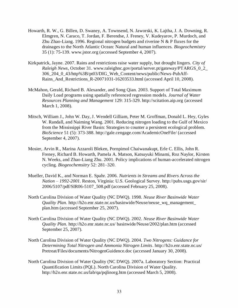
Table A.1. Attributes included in pySPARROW database .............................................................. 36
Table A.2. Observed and predicted total nitrogen concentrations................................................... 37
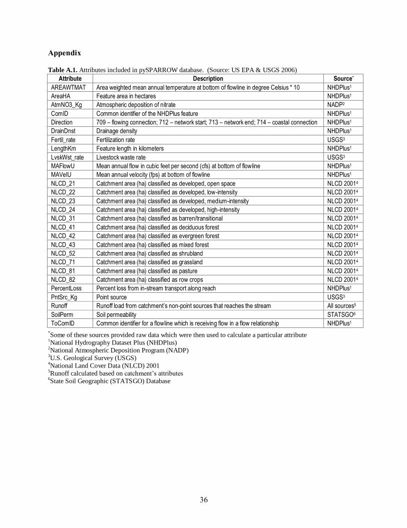
Table A.3. NLCD 1992 and 2001 land cover change matrix .......................................................... 38

iii
Acknowledgements
I would like to thank Dr. Dean Urban, my master’s project advisor, for his vital guidance
and encouragement. Many thanks to John Fay for helping me better understand Python and
pySPARROW and for patiently answering all of my technical questions. I would like to thank
Dr. Jon Goodall for his pySPARROW assistance and David Vinson for providing total nitrogen
references. A big thanks to the Assessment of US Habitat Conservation and Provision of
Ecosystem Services project, which is funded by the National Council for Science and the
Environment as part of their Wildlife Habitat Policy Research Program, for funding this
research. Finally, many thanks to my family and friends for their unending support and
motivation.

1
1. Introduction
Ecosystems provide vital benefits to humans, plants, and animals ranging from
preserving biodiversity to generating soil (Prato 2007). These services are of extreme
importance to society and have an estimated economic value of about $33 trillion per year for the
entire biosphere (Costanza et al. 1997). In particular, many of these benefits influence water
quality and quantity. For example, floodplains, wetlands, and riparian buffers help purify and
supply water, provide flood and erosion control, and maintain groundwater supplies (Federal
Interagency Floodplain Management Task Force 1992; Chan et al. 2006; Verhoeven et al. 2006).
Land use and land cover changes, however, may compromise many of these watershed
services. For instance, land converted to agricultural or urban uses may have increased erosion,
runoff, or flooding (Prato 2007). Furthermore, land use modifications may degrade water
quality. In particular, the nitrogen loading of a waterbody may be influenced by the land cover
of its drainage area because different land covers are likely to be sources or sinks of nitrogen.
For example, wetlands and forests tend to store nitrogen while agricultural and urban lands tend
to be sources of nitrogen (Howarth et al. 2000). Wetlands and forests may retain nitrogen over
the long-term in vegetation and soil organic matter and buffer streams from nonpoint source
pollution (Mosier et al. 2001). Croplands and pastures may increase the levels of nitrogen in
waterbodies through the runoff of surplus fertilizer and livestock manure, the cultivation of
nitrogen-fixing crops, and the plowing of agricultural lands (see, for example, Howarth et al.
1996; Worrall and Burt 1999; Houlahan and Findlay 2004; Verhoeven et al. 2006). Developed
areas may also increase the nitrogen loading through the various point and nonpoint sources
associated with urban land. For instance, significant anthropogenic nitrogen sources include:
fossil fuel combustion, which deposits nitrogen in the atmosphere; municipal wastewater, which
2
is the principal point source of nitrogen in U.S. waterbodies; and runoff from impervious
surfaces (Howarth et al. 1996; Howarth et al. 2000; Mitsch et al. 2001).
Anthropogenic sources of nitrogen, such as those associated with agricultural and urban
land uses, have significantly affected the nitrogen cycle by doubling the amount of biologically
available nitrogen (Mosier et al. 2001). Across the globe, land is being converted from land
covers that tend to store nitrogen to uses that are associated with nitrogen sources. Over the past
three hundred years, croplands have increased by 12 million km2 worldwide through conversions
of forests and grasslands (Ramankutty and Foley 1999). Urbanized land is also increasing. For
example, between 1982 and 1997, 121,000 km2 of land in the U.S. were developed (Prato 2007).
Excess nitrogen reaching waterbodies from agricultural or urban lands may result in
eutrophication, increased levels of nitrates in groundwater, and microbial problems (Berka et al.
2001).
By testing the physical and chemical characteristics of water, researchers may examine
the relationship between land use changes and water quality and determine which waterbodies
are failing to meet water quality standards. Under the Clean Water Act, states must identify
impaired waterbodies on a state 303(d) List and implement total maximum daily load (TMDL)
programs for contaminated waterbodies. TMDLs, a calculation of the maximum amount of a
pollutant that a waterbody can receive while still meeting water quality standards, are used to
restore water quality by controlling point and nonpoint contaminant sources. States have
identified nearly 500,000 kilometers (km) of impaired rivers and shorelines and 2 million
hectares (ha) of contaminated lakes (McMahon et al. 2003).
While testing water quality to examine the effects of land cover changes on water quality
is extremely important, monitoring can be expensive and time consuming so it is unrealistic to
gather data for all of the streams in the U.S. Furthermore, watershed managers need tools to

3
develop TMDL programs. To address these problems, researchers have developed a wide
variety of hydrologic models to extrapolate from sampled locations to unsampled locations and
to predict nutrient loadings under scenarios with varying nutrient sources and landscape
properties. These models differ in their complexity and the temporal and spatial scales they use
to describe nutrient sources and flow through watersheds. Water quality models generally fall on
a continuum with statistical models on one side and deterministic models on the other (fig. 1.).
Purely statistical models are
simple linear regressions that
correlate observed water
quality data with nutrient
sources and land-surface
characteristics. In contrast,
deterministic models, such as
SWAT (Soil Water
Assessment Tool) and HSPF (Hydrologic Simulation Program – Fortran), tend to be more
complex with finer temporal and spatial scales (Schwarz et al. 2006).
This project evaluates an application of the U.S. Geological Survey’s SPARROW
(Spatially Referenced Regressions on Watershed Attributes) model. SPARROW estimates total
nitrogen and total phosphorus loads for watersheds by relating water quality information to
nutrient sources, landscape properties, stream connectivity, and downstream travel time (Smith et
al. 1997). As shown in Figure 1, SPARROW uses a hybrid approach to describe water quality
because it is a nonlinear regression model that works in a geospatial framework (Schwarz et al.
2006).
Figure 1. Continuum of water quality models. Water quality models
generally fall on a continuum between statistical models, which are simpler,
and deterministic models, which have more complex model processes and
finer temporal and spatial scales. (Source: Schwarz et al. 2006.)

4
The primary objective of this project was to assess pySPARROW, an application of
SPARROW written in the Python programming language for North Carolina's non-tidal stream
network. pySPARROW was developed in May of 2007 by Jon Goodall and Dave Bollinger so it
is still being frequently updated. By comparing the estimated total nitrogen concentrations of
several catchments in the Falls Lake subbasin with observed water quality data, this project
evaluates how well pySPARROW predicts the long term mean total nitrogen concentration. The
model was also used to assess watershed impacts of a development scenario under which forest
and agricultural lands were converted to urban land uses. Improving the accuracy of this model
and making it available to the public is important so that watershed managers and policymakers
may identify which watersheds are most sensitive to land cover changes and may better plan for
meeting water quality standards with the projected development in their region.
2. Study Area and Model Scenarios
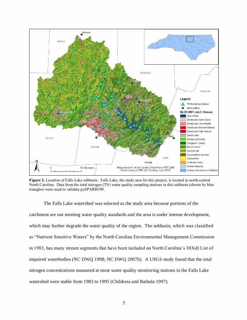
The Falls Lake subbasin was selected as the study area (fig. 2). Falls Lake is located in
the Upper Neuse River Basin in north-central North Carolina. This watershed is nearly 2,000
km2, with about 83 km
2 in water and the remaining area in land. Around 73 percent of the
subbasin is covered in forests and wetlands, 14 percent is pastureland, seven percent is urban
land uses, and three percent is cultivated crops (NC DWQ 2002). Falls Lake contains at least
part of eight municipalities, with the City of Durham and the Town of Hillsborough being the
two notably developed areas in the watershed. The subbasin also falls within the jurisdiction of
six counties. Around 66 percent of the households in the watershed are found in Durham
County, of which about 40 percent are found in the City of Durham (UNRBA 2003). The
estimated population density for Falls Lake is around 100 people/km2
(NC DWQ 2002).
5
The Falls Lake watershed was selected as the study area because portions of the
catchment are not meeting water quality standards and the area is under intense development,
which may further degrade the water quality of the region. The subbasin, which was classified
as “Nutrient Sensitive Waters” by the North Carolina Environmental Management Commission
in 1983, has many stream segments that have been included on North Carolina’s 303(d) List of
impaired waterbodies (NC DWQ 1998; NC DWQ 2007b). A USGS study found that the total
nitrogen concentrations measured at most water quality monitoring stations in the Falls Lake
watershed were stable from 1983 to 1995 (Childress and Bathala 1997).
Figure 2. Location of Falls Lake subbasin. Falls Lake, the study area for this project, is located in north-central North Carolina. Data from the total nitrogen (TN) water quality sampling stations in this subbasin (shown by blue
triangles) were used to validate pySPARROW.

6
The major nitrogen sources of this subbasin are urban runoff, agricultural runoff, and
failing septic tanks. Treated municipal wastewater is also discharged into Falls Lake. Because
of these nitrogen sources, eutrophication threatens the lakes in this region. Eutrophication,
which may be caused by an increase in nitrogen reaching bodies of water, promotes algal
blooms, which in turn may deplete the oxygen in the water on which aquatic life rely. Algal
blooms may also influence the recreational uses of lakes by limiting boating and fishing
opportunities. Further downstream, the aquatic life and recreational and commercial uses of the
Neuse Estuary have been impaired due to eutrophication. Eutrophication may also affect
drinking water quality by causing taste and odor problems and an increased risk of toxics from
algal blooms (UNRBA 2003). The Falls Lake subbasin contains nine drinking water supply
reservoirs, with Falls Lake being the primary water supply of Raleigh (UNRBA 2003;
Kirkpatrick 2007). Altogether, it is estimated that this subbasin supplies water for around
450,000 residents, so protecting the water quality of this region is extremely important (UNRBA
2003).
Falls Lake was also selected as the study area because it is rapidly developing. The
population of the subbasin increased by 21 percent from 1990 to 2000 and is projected to
increase an additional 53 percent between 2000 and 2025 (UNRBA 2003). Given this expected
population growth, over 280 km2 of forests and agricultural land in the Falls Lake watershed are
expected to be developed into residential and urban uses by 2025 (UNRBA 2003). Therefore,
estimating the effects of this increasing urbanized land on the nitrogen loads for this region is
especially important for watershed managers. Furthermore, planning to meet water quality
standards may be complicated by development so it is essential for these managers and planners
to have a hydrologic model to predict how development may affect water quality and to mitigate
these potential impacts.
7
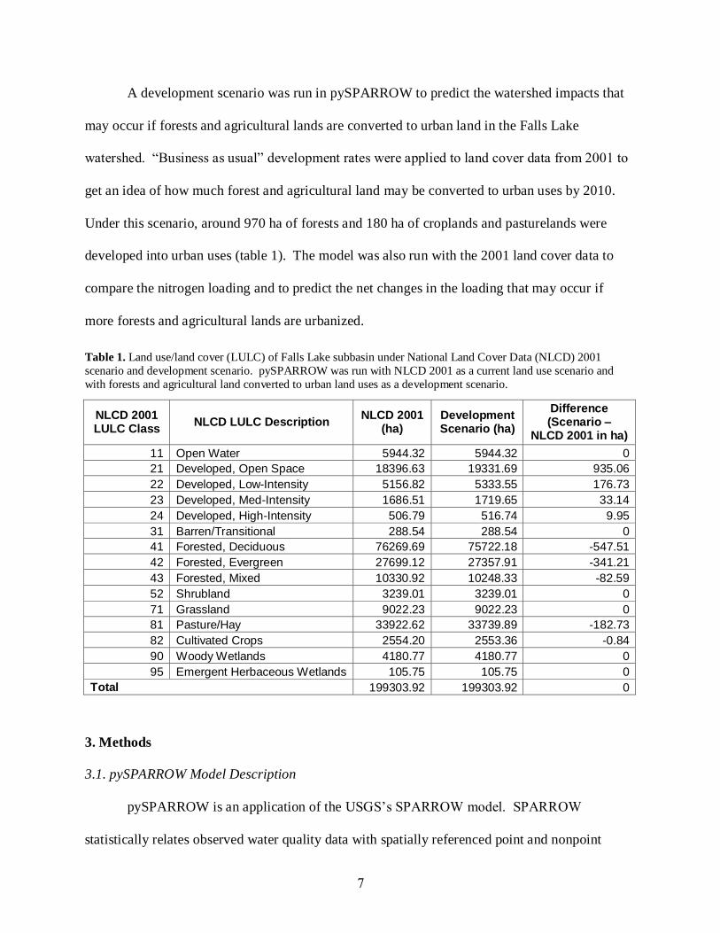
A development scenario was run in pySPARROW to predict the watershed impacts that
may occur if forests and agricultural lands are converted to urban land in the Falls Lake
watershed. “Business as usual” development rates were applied to land cover data from 2001 to
get an idea of how much forest and agricultural land may be converted to urban uses by 2010.
Under this scenario, around 970 ha of forests and 180 ha of croplands and pasturelands were
developed into urban uses (table 1). The model was also run with the 2001 land cover data to
compare the nitrogen loading and to predict the net changes in the loading that may occur if
more forests and agricultural lands are urbanized.
Table 1. Land use/land cover (LULC) of Falls Lake subbasin under National Land Cover Data (NLCD) 2001
scenario and development scenario. pySPARROW was run with NLCD 2001 as a current land use scenario and
with forests and agricultural land converted to urban land uses as a development scenario.
NLCD 2001 LULC Class
NLCD LULC Description NLCD 2001
(ha) Development Scenario (ha)
Difference (Scenario –
NLCD 2001 in ha)
11 Open Water 5944.32 5944.32 0
21 Developed, Open Space 18396.63 19331.69 935.06
22 Developed, Low-Intensity 5156.82 5333.55 176.73
23 Developed, Med-Intensity 1686.51 1719.65 33.14
24 Developed, High-Intensity 506.79 516.74 9.95
31 Barren/Transitional 288.54 288.54 0
41 Forested, Deciduous 76269.69 75722.18 -547.51
42 Forested, Evergreen 27699.12 27357.91 -341.21
43 Forested, Mixed 10330.92 10248.33 -82.59
52 Shrubland 3239.01 3239.01 0
71 Grassland 9022.23 9022.23 0
81 Pasture/Hay 33922.62 33739.89 -182.73
82 Cultivated Crops 2554.20 2553.36 -0.84
90 Woody Wetlands 4180.77 4180.77 0
95 Emergent Herbaceous Wetlands 105.75 105.75 0
Total 199303.92 199303.92 0
3. Methods
3.1. pySPARROW Model Description
pySPARROW is an application of the USGS’s SPARROW model. SPARROW
statistically relates observed water quality data with spatially referenced point and nonpoint

8
contaminant sources, land-surface characteristics, and stream characteristics. To predict total
nitrogen, the national SPARROW model uses 18 parameters (Schwarz et al. 2006).
The first set of parameters describes loads from upstream basins and pollutant inputs that
drain directly to a catchment (Preston and Brakebill 1999). These source parameters include
point sources, atmospheric deposition, fertilizer use, livestock waste, forestland, grassland,
shrubland, transitional land, and urban land (Schwarz et al. 2006).
The second set of parameters describes landscape properties that influence the delivery of
nutrients from land to water (Preston and Brakebill 1999). Soil permeability, drainage density,
and temperature are land-to-water delivery factors used in SPARROW. For example,
catchments with more impervious surfaces tend to increase the delivery of nutrients from land
surfaces to waterbodies (Schwarz et al. 2006).
Finally, the third set of parameters describes stream decay. As nutrients travel
downstream, stream processes, such as denitrification, usually cause a portion of the
contaminants to decay (Preston and Brakebill 1999). This in-stream loss is a function of
downstream travel time, channel depth, and whether or not a stream segment is part of a
reservoir. For instance, deeper streams tend to have lower rates of decay because the major in-
stream loss processes occur at the bottom of the stream channel (Smith et al. 1997).
These three sets of parameters are the independent variables that are related in a nonlinear
regression model to estimate the total nitrogen loading. Observed water quality data is used as
the dependent variable to calibrate SPARROW (Preston and Brakebill 1999).
The pySPARROW model uses the same parameters and coefficients as SPARROW.
There are, however, three major differences between SPARROW and pySPARROW.
First, SPARROW was written in the Statistical Analysis System (SAS) language, while
pySPARROW was developed in the Python programming language (Schwarz et al. 2006).

9
pySPARROW was written in Python for two predominant reasons. First, the geoprocessor
object of ArcGIS 9.2 allows Python scripts to execute ArcGIS geoprocessing functions and tools.
Therefore, because the model is in Python, Python scripts may be written to create ArcGIS tools
that use pySPARROW. Creating tools that use this model is important so that pySPARROW
internet tools may be developed and shared with watershed managers and planners. Second,
pySPARROW was written in Python so that it may use the Python module NetworkX, a library
of network analysis functions (Hagberg et al. 2006). By using NetworkX, the stream network of
pySPARROW was constructed as a hydrologic network so that the model may be used to
identify which streams segments are upstream or downstream from a particular stream.
A second difference between SPARROW and pySPARROW is the geographic region
and nutrients that each model predicts. SPARROW estimates the long-term, steady-state total
nitrogen and total phosphorus loading for the non-tidal continental U.S. (Schwarz et al. 2006).
At this point in time, pySPARROW has only been developed to predict the long-term, average
total nitrogen loading and concentration for non-tidal North Carolina, but the model can, and
hopefully will, be
expanded to cover a larger
geographic region in the
future (fig. 3). Because
the stream network of
pySPARROW was
developed as a hydrologic
network, it does not
currently predict the Figure 3. Region covered by pySPARROW. Currently, pySPARROW has been
developed to predict the long-term, mean total nitrogen loading and
concentration for non-tidal North Carolina (region shaded in blue).

10
nutrient loading for the western portion of North Carolina, which drains to the Gulf of Mexico
while the rest of the state drains to the Atlantic Ocean. pySPARROW has also not yet been
developed to estimate total phosphorus.
Finally, the spatial resolution of SPARROW and pySPARROW differ. SPARROW uses
the U.S. Environmental Protection Agency’s (EPA) Reach File 1 (RF1) data at a 1:500,000 scale
while pySPARROW uses the USGS and EPA’s 1:100,000 National Hydrography Dataset Plus
(NHDPlus) data (fig. 4)
(Schwarz et al. 2006; US
EPA 2006). By using
higher resolution stream
data, pySPARROW has
the potential to describe
water quality at a much
finer scale than
SPARROW.
pySPARROW is
a fairly straightforward
model to use. To run
pySPARROW, users must have the pySPARROW database and Python script and the module
dependencies of pySPARROW, such as NetworkX, on their computers. The database includes
attributes for 96,201 stream segments, 1,600 of which are located in the Falls Lake subbasin, that
make up the hydrologic network of NHDPlus flowlines for which pySPARROW predicts the
nitrogen loading. These spatially referenced attributes are the parameters that are related to
Figure 4. Comparison of data resolution used for SPARROW and
pySPARROW. SPARROW uses the EPA’s Reach File 1 (RF1) data for its
stream network while pySPARROW uses the USGS and EPA’s National
Hydrography Dataset Plus (NHDPlus). By using higher resolution data,
pySPARROW may describe the total nitrogen loading at a finer spatial scale
than SPARROW.

11
predict the total nitrogen loading and concentration (table A.1). For this project, the database file
data_v400.h5 was used.
The pySPARROW script includes functions that are used to relate the parameters to
calculate water quality. The script includes four objects: the database, reach, network, and
waterbody classes. The database class allows users to do such functions as open, close, create, or
delete a table. Tables may be created, for example, so that land use modifications may be saved
to a new table. The reach object is the most basic spatial unit in pySPARROW. A reach is a
stream channel between two tributary junctions (fig. 5) (Schwarz et al. 2006). A unique
common identifier (ComID)
is assigned to each NHDPlus
flowline segment and its
corresponding catchment,
which is the area of land that
drains to the reach. The
attributes of the database are
assigned to each reach. A
user may get the land use
and land cover (LULC), set
the LULC, get the runoff
load, or get the concentration of a reach. The network class is set of reaches connected into a
graph. This object allows users to identify upstream or downstream reaches of a particular river
segment. Finally, the waterbody object is a reach that receives contaminants from upstream river
segments. The total nitrogen loading or concentration may be calculated for a waterbody. For
this project, version 0.301 of the pySPARROW script was used.
Figure 5. Illustration of a reach network. Stream reaches are the most basic
spatial unit in pySPARROW. pySPARROW predicts the total nitrogen
loading and concentration for individual reaches and incremental
waterbodies. (Source: Schwarz et al. 2006.)
12
3.2. pySPARROW Model Validation
pySPARROW was first validated to assess how well the model predicts the long-term,
mean total nitrogen concentration. To validate pySPARROW, the observed total nitrogen
concentrations for monitoring stations in the Falls Lake watershed were plotted against the
predicted concentrations. The observed total nitrogen data were based on all of the available
water quality data that met certain criteria that were used by the developers of SPARROW. In
particular, data from a monitoring station were used to calibrate SPARROW only if there were at
least 15 water quality observations taken at the station between 1970 and 2000 (Schwarz et al.
2006). Therefore, to validate pySPARROW, all available data from stations in the Falls Lake
subbasin with at least 15 total nitrogen observations from 1970 to 2000 were used (see fig. 2 for
the locations of the total nitrogen water quality sampling sites). Total nitrogen data from 47
monitoring stations in Falls Lake met these criteria. The observed data were from the EPA’s
STORET (Storage and Retrieval) data system and the USGS’s National Water Information
System (NWIS).
Total nitrogen consists of organic nitrogen, ammonia nitrogen, nitrite, and nitrate (NC
DWQ 2004). To calculate the total nitrogen concentration from the STORET data, total Kjeldahl
nitrogen, which is equal to organic nitrogen plus ammonia nitrogen, was added to nitrite and
nitrate (NC DWQ 2004). NWIS includes water quality data for both filtered and unfiltered water
samples. For this study, the filtered total nitrogen concentrations were used to validate
pySPARROW because the nitrogen data used to calibrate SPARROW were from filtered
samples (Mueller and Spahr 2006; Schwarz et al. 2006).
pySPARROW was then run to find the predicted total nitrogen concentration. In
ArcGIS, the ComIDs of the catchments in which the 47 monitoring stations were located were
identified. pySPARROW was then run for each of these catchments. Finally, the observed total

13
nitrogen concentrations were plotted against the predicted concentrations (see table A.2 for the
data used in the regression analysis).
A regression analysis of the observed versus predicted total nitrogen concentration shows
that pySPARROW most likely needs to be recalibrated (fig. 7). The regression analysis has a
probability value of 0.14 and an adjusted R-squared value of 0.03. A map of log residuals shows
the predicted minus the observed total nitrogen concentration values for the water quality
monitoring sites in Falls Lake (fig. 6). pySPARROW tends to under-predict the concentration.
The model over-predicted nine out of the 47 stations and under-predicted the other 38 stations.
The highest the model over-estimated the total nitrogen concentration was by 0.5 milligrams per
Figure 6. Log residuals (predicted minus observed total nitrogen concentration values). Data from these 47 water
quality monitoring stations in Falls Lake were used to validate pySPARROW.

14
liter (mg/L). The model under-
predicted 15 stations by less than 0.5
mg/L, 15 sites by between 0.5 mg/L
and 1.0 mg/L, and eight stations by
greater than 1.0 mg/L. The most the
model under-estimated was by 15.47
mg/L.
A second regression analysis
was run with only those stations in the
Falls Lake subbasin that had at least
two years of observations, 24 or more
observations, and an observed mean
total nitrogen concentration of 2.0
mg/L or less (fig. 8). The developers
of SPARROW recommended that
water quality data meet these first two
criteria so stations that did not meet
these suggestions were removed to
reduce biased observations (Schwarz
et al. 2006). Eight of the 47 stations
were removed because they did not
have samples over at least two years or
24 or more observations. An
Figure 7. Observed versus predicted total nitrogen concentration
(mg/L) for the monitoring stations in the Falls Lake subbasin with
at least two years of observations, 24 or more observations, and
mean concentrations less than 2.0 mg/L. This regression analysis
has a probability value of 0.003 and an adjusted R-squared value
of 0.19.
Figure 8. Observed versus predicted total nitrogen concentration
(mg/L) for the Falls Lake subbasin. This regression analysis has a probability value of 0.14 and an adjusted R-squared value of 0.03.
Figure 7. Observed versus predicted total nitrogen concentration
(mg/L) for the Falls Lake subbasin. This regression analysis has a probability value of 0.14 and an adjusted R-squared value of 0.03.
Figure 8. Observed versus predicted total nitrogen concentration
(mg/L) for the monitoring stations in the Falls Lake subbasin with
at least two years of observations, 24 or more observations, and
mean concentrations less than 2.0 mg/L. This regression analysis
has a probability value of 0.003 and an adjusted R-squared value
of 0.19.

15
additional seven stations were removed for this analysis because they had mean concentrations
above 2.0 mg/L with mean concentrations ranging from 4.04 mg/L to 16.27 mg/L. The results
from this analysis have a probability value of 0.01 with an adjusted R-squared of 0.18. For this
project, relative changes in the total nitrogen loading, rather than absolute changes, will be
compared under current land use and a development scenario.
3.3 Current Land Use Scenario
To calculate the net changes that may occur in Falls Lake if forests and agricultural lands
are developed, pySPARROW was run with a current land use scenario using National Land
Cover Data (NLCD) from 2001. This dataset was developed by the Multi-Resolution Land
Characteristics (MRLC) Consortium, a group of federal agencies (US DOI and USGS 2008b).
The NLCD 2001
data includes 21
land use and land
cover classes at a
30 meter cell
resolution. A
shapefile of the
1,600 NHDPlus
catchments
located in the Falls
Lake watershed
was converted to a Figure 9. Current land use (NLCD 2001). A current land use scenario was run with the
National Land Cover Data (NLCD) from 2001. The NLCD 2001 data includes 21 land
use and land cover (LULC) classes at a 30 meter cell resolution.

16
raster and then combined with the NLCD 2001 raster (fig. 9). A script was used to create a new
table in the pySPARROW database and to update this table for each catchment in the study area
to include the number of hectares of each land cover class according to the NLCD 2001 data.
The model was then run to find the total nitrogen loading of Falls Lake in kilograms per year (kg
N/yr) and the relative contribution of each of the 1,600 catchments to the total loading.
3.4 Development Scenario
A development scenario was then run in pySPARROW to assess the potential watershed
impacts that may occur if forests and agricultural lands are urbanized. NLCD is available for
both 1992 and 2001. The MRLC Consortium, however, recommends that users do not directly
compare these two products. Slightly different classifications were used for these two datasets
so some perceived changes over these nine years may be due to changes in the classification
technique rather than actual change (US DOI and USGS 2008a). To address this problem, the
MRLC Consortium developed the NLCD 1992/2001 Retrofit Land Cover Change Product. To
produce this dataset, the data from1992 and 2001 were both reclassified using Anderson Level I
land use and land cover classes. Anderson Level I classes are more generalized than the
Anderson Level II classes that were used in the NLCD 1992 and 2001 products. For example,
the NLCD 2001 data differentiates cultivated crops from pasture and hay, while the land cover
change dataset consolidates these land uses into a generalized agriculture class.
The 1992/2001 land cover change data were used to calculate what percentage of forests
and agricultural land were converted to urban uses between 1992 and 2001 for each catchment in
the study area. The land cover change raster was combined with a raster of the NHDPlus
catchments in Falls Lake (fig. 10). As shown in figure 10, all the blue highlighted areas are
locations where the land cover was modified between 1992 and 2001. For this study, only those

17
areas where forests and agricultural lands were converted to urban uses were considered (fig.
11).
Figure 10. Forest and agricultural lands urbanized between 1992 and 2001. For each
catchment in Falls Lake, the percentage of the area of forests and agricultural lands that
were urbanized between 1992 and 2001 was found and this same percentage was then
developed between 2001 and 2010 under the development scenario.
Figure 11. NLCD 1992/2001 land cover changes. All of the blue highlighted areas are
locations where the land cover was modified between 1992 and 2001.
Figure 11. Forest and agricultural lands urbanized between 1992 and 2001. For each
catchment in Falls Lake, the percentage of the area of forests and agricultural lands that
were urbanized between 1992 and 2001 was found and this same percentage was then
developed between 2001 and 2010 under the development scenario.
Figure 10. NLCD 1992/2001 land cover changes. All of the blue highlighted areas are
locations where the land cover was modified between 1992 and 2001.

18
The data from the combined raster were then exported to Microsoft Access. In Access,
the percentage of all of the pixels classified as forests in 1992 that were converted to urban uses
in 2001 was found for each catchment. The percentage of the area of agricultural land that was
urbanized between 1992 and 2001 was also calculated for each catchment. A total of 310
catchments had forests developed and 186 catchments had agricultural land urbanized from 1992
to 2001. Under the development scenario, the same percentage of forests and agricultural land
that were developed between 1992 and 2001 are urbanized from 2001 to 2010. The percentage
of forests converted to urban uses ranges from 0.03 percent to 100 percent and the percentage of
agricultural land developed ranges from 0.02 percent to 100 percent under the development
scenario.
The number of hectares developed was calculated for each catchment. For those
catchments with conversions from forests to urban uses, equal percentages of hectares were
subtracted from each of the three forest classes (i.e., deciduous, evergreen, and mixed forests).
pySPARROW adds the area of these three Anderson Level II forest classes so different
percentages did not need to be subtracted from these classes. pySPARROW does, however,
differentiate between the Anderson Level II agricultural classes (i.e., cultivated crops and
pasture/hay). The area of cultivated crops is used to calculate the fertilization runoff while the
area of pasture and hay is used to estimate the runoff of livestock waste. According to the U.S.
Department of Agriculture’s 2002 Census of Agriculture, land used for pastures and hay
decreased between 1992 and 2002 in North Carolina while the area of cultivated crops increased
in the state during this time period (USDA 2004). Therefore, the area of agricultural lands
developed was subtracted from the area of pasture and hay in each catchment. Three
catchments, however, did not have any pasture and hay land so the area developed was
subtracted from the area of cultivated crops.

19
Next, the hectares subtracted from the forests and agricultural land covers were added to
the developed land uses. pySPARROW uses different coefficients for the urban Anderson Level
II classes. In particular, pySPARROW treats developed open space land as grassland and
developed low-, medium-, and high-intensity land as urban land. To calculate what percentage
of the developed forests and agricultural land should be converted to each of the four urban
classes, a change matrix was created for a random one percent sample of the NLCD 1992 and
2001 data in Falls Lake (table A.3). The same percentage of forests and agricultural lands that
were converted to each of the four urban uses from 1992 to 2001 were converted under the
development scenario. Of the forest land changed to urban uses under the development scenario,
around 82 percent was converted to developed open space, 14 percent to developed low-
intensity, three percent to developed medium-intensity, and one percent to developed high-
intensity. For the urbanized agricultural land, around 85.9 percent was converted to developed
open space, 13.7 percent to developed low-intensity, and 0.4 percent to developed medium-
intensity. Overall, the land uses of 378 catchments in the Falls Lake subbasin were modified and
slightly less than one percent of the all of the forests and around 0.5 percent of the agricultural
land were urbanized in the study area under the development scenario.
These changes in the land uses were incorporated into a new table in the pySPARROW
database using a script. The model was then run to find the total nitrogen loading of the Falls
Lake watershed under this development scenario and the relative contribution of each of the
catchments in the study area.
4. Results
Under the development scenario, the total nitrogen loading was predicted to increase by
0.23 percent from around 908,855 kg N/yr to 910,952 kg N/yr (fig. 12). Under the current land

20
use scenario, a catchment in Hillsborough was the largest contributor of the total loading of the
watershed by supplying 5.5 percent of the total nitrogen load. The second largest contributing
catchment, responsible for 4.4 percent of the total loading, was located in the City of Durham.
The seven catchments that contribute the largest percentages of the total loading were all located
in Hillsborough or Durham. Under the development scenario, these same seven catchments
remained the largest suppliers of nitrogen.
The percentage values of each catchment under the current land use scenario were
subtracted from the percentage values under the development scenario to find the relative
percentage change of what each catchment is contributing to the total loading, (fig. 13). A total
of 1,313 catchments had a decrease in the percentage that they contribute to the total loading, 39
catchments had no change, and 248 catchments had an increase in the percentage that they
Figure 12. Percentage that each catchment contributes to the total loading of the Falls Lake subbasin under current land use (NLCD 2001) (A) and the development scenario (B). Under both scenarios, the seven catchments
that contribute the greatest share of the nitrogen load are located in the Town of Hillsborough and the City of
Durham.

21
contribute to the total loading. A 0.014 percent increase was the largest percentage increase
estimated under the development scenario. The two largest percentage increases occurred in
Hillsborough, the third greatest increase took place in a catchment located in the outskirts of the
City of Durham, the fourth largest increase was estimated along Interstates 40 and 85 in the
south-western edge of the study area, and the fifth greatest increase was predicted along
Interstate 85, which runs northward through the center of the watershed. A 0.007 percent
decrease was the maximum decline in the percentage that a catchment contributed to the total
nitrogen loading of Falls Lake. The five catchments with the greatest declines in percentages
Figure 13. Relative percentage change (percentage values of each catchment under the development scenario minus
percentage values under current land use). A total of 1,313 catchments had a decrease in the percentage of the total
loading that they contribute (shown in blue), 39 catchments had no change (shown in green), and 248 catchments
had an increase in the percentage of the total loading that they contribute (shown in orange and red) under the
development scenario.

22
were all located in the Town of Hillsborough or the City of Durham.
The relative change in the total nitrogen loading of each catchment was also calculated
(fig. 14). The total nitrogen load of each catchment under the current land use scenario was
subtracted from the total nitrogen load under the development scenario. Of the 378 catchments
that experienced land cover conversions under the development scenario, five catchments were
predicted to have a decrease in the nitrogen loading under the development scenario and 373
catchments were estimated to have an increase in their loads. All five of the catchments that
were predicted to have a decrease in their loadings were estimated to have a decrease of 0.05 kg
Figure 14. Relative total nitrogen loading change (total nitrogen load under the development scenario minus load
under current land use). Of the 378 catchments that experienced land cover conversions under the development
scenario, five catchments were predicted to have a decrease in the nitrogen loading under the development scenario
(shown in blue) and 373 catchments were estimated to have an increase in their loads (shown in red).

23
N/yr or less. The catchment with the greatest predicted increase in its total nitrogen loading (an
estimated increase of 173.73 kg N/yr) was located in Hillsborough. Three of the five catchments
with the largest increases in their nitrogen loadings were located in Hillsborough.
Under the development scenario, 192 catchments had just forests developed, 67
catchments had just agricultural lands urbanized, and 119 catchments had both forests and
agricultural lands developed (fig. 15). Of the 192 catchments with just forests converted, only
one was predicted to have a decrease in its total nitrogen loading under the development
scenario, while all of the other catchments were predicted to experience an increase. Four of the
67 catchments that lost just agriculture to urban uses experienced a decrease in their total
nitrogen loadings, while the remaining 63 catchments were predicted to have an increase.
Finally, all of the catchments with both forests and agricultural lands developed had an increase
in their total nitrogen loadings.
Figure 15. Comparison of relative loading change for catchments with development of just forests (A), catchments with development of just agricultural lands (B), and catchments with development of both forests and agricultural
lands (C). All but one of the 192 catchments with just forests developed were predicted to have an increase in their
total nitrogen loading under the development scenario. All but four of the 67 catchments with just agricultural land
developed were predicted to have an increase in their total nitrogen loading under the development scenario. All
119 catchments with both forests and agricultural lands developed were predicted to have an increase in their total
nitrogen loadings.

24
5. Discussion
The results from the regression analysis used to validate pySPARROW show that the
model probably should be recalibrated to more accurately predict total nitrogen (fig. 7). Many of
the predicted values were less than the practical quantification limit (PQL), a reliable detection
level, for nitrogen. As mentioned above, total nitrogen is the sum of total Kjeldahl nitrogen
(TKN), nitrite, and nitrate. According to the North Carolina Division of Water Quality, the PQL
for TKN as nitrogen is 0.20 mg/L and for nitrite and nitrate as nitrogen is 0.01 mg/L (NC DWQ
2007a). Therefore, seven of the 47 predicted total nitrogen concentrations for the monitoring
sampling sites were less than the detectable level for nitrite and nitrate and 25 of the predicted
concentrations were less than the PQL for TKN (table A.3). All seven of the stations that had
estimated concentrations below the PQL for nitrite and nitrate had seven or fewer catchments
that contributed to their total nitrogen loading. In contrast, the monitoring site with the second
highest predicted concentration of 1.06 mg/L had 1,584 upstream catchments. While these
results suggest that the predicted concentration may be strongly correlated to the number of
upstream catchments, there were some exceptions. For example, the monitoring site with the
highest predicted total nitrogen concentration of 1.86 mg/L only had 46 contributing reaches. If
pySPARROW were calibrated to statistically relate the observed water quality to the parameters,
then it may more accurately predict the total nitrogen loading and concentration of catchments
with fewer upstream catchments. Furthermore, pySPARROW under-estimated the total nitrogen
concentration for 30 of the 31 sampling sites that had fewer than 500 upstream catchments. For
the 16 sites that had more than 500 upstream catchments, pySPARROW under-estimated the
concentration of eight of these sites.
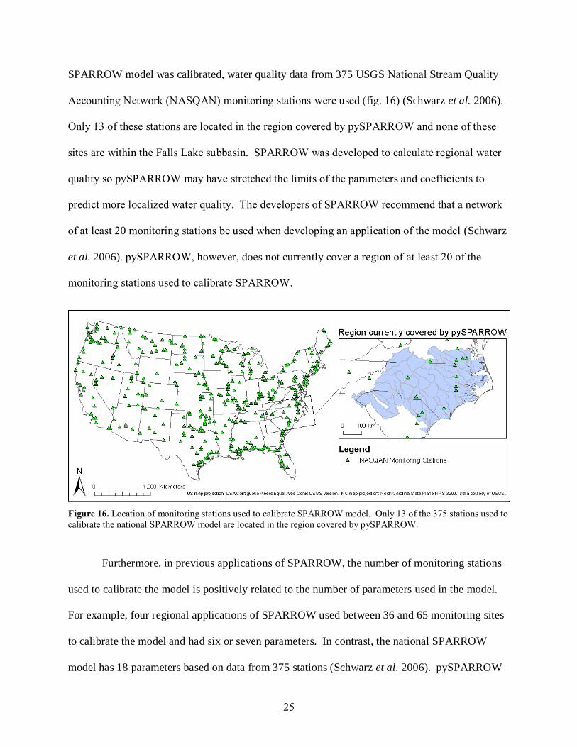
Overall, the regression analysis shows that applying the SPARROW parameters and
coefficients to the higher resolution NHDPlus data reduces the accuracy of the model. When the
25
SPARROW model was calibrated, water quality data from 375 USGS National Stream Quality
Accounting Network (NASQAN) monitoring stations were used (fig. 16) (Schwarz et al. 2006).
Only 13 of these stations are located in the region covered by pySPARROW and none of these
sites are within the Falls Lake subbasin. SPARROW was developed to calculate regional water
quality so pySPARROW may have stretched the limits of the parameters and coefficients to
predict more localized water quality. The developers of SPARROW recommend that a network
of at least 20 monitoring stations be used when developing an application of the model (Schwarz
et al. 2006). pySPARROW, however, does not currently cover a region of at least 20 of the
monitoring stations used to calibrate SPARROW.
Furthermore, in previous applications of SPARROW, the number of monitoring stations
used to calibrate the model is positively related to the number of parameters used in the model.
For example, four regional applications of SPARROW used between 36 and 65 monitoring sites
to calibrate the model and had six or seven parameters. In contrast, the national SPARROW
model has 18 parameters based on data from 375 stations (Schwarz et al. 2006). pySPARROW
Figure 16. Location of monitoring stations used to calibrate SPARROW model. Only 13 of the 375 stations used to
calibrate the national SPARROW model are located in the region covered by pySPARROW.

26
uses the same parameters as the national model so recalibrating pySPARROW’s coefficients
with data from a regional network of monitoring stations would be expected to improve the
accuracy of the model.
There were several limitations to the methods used to validate pySPARROW. The
observed water quality data used to validate the model was likely biased. Water quality samples
are often sparse, due to the high cost of monitoring. Samples may also be unrepresentative
because locations that are suspected of having water quality problems tend to be monitored
(Schwarz et al. 2006). The data used to validate pySPARROW were no exception. As shown in
Table A.3, the stations with the two highest observed total nitrogen concentrations (J1269000
and J1280000) were only sampled over the course of two years. This short sampling period and
high mean concentration suggest that these stream segments may have experienced specific
water quality problems. Furthermore, biases may also exist in when samples were taken. If
most of the samples were collected during one particular season, then the calculated average total
nitrogen concentration may be higher or lower than the long-term mean. For instance, one
station’s data used to validate pySPARROW had few samples from the fall, while another station
had a smaller percentage of samples from the summer. Finally, the locations of the sampling
sites may also be biased. As shown in figure 2, most of the water quality monitoring stations
were located in the southern portion of the subbasin and are concentrated around Falls Lake.
A second regression analysis was run to try to remove some biases by using only those
stations in the Falls Lake subbasin that had at least two years of observations, 24 or more
samples, and a concentration less than 2.0 mg/L (fig. 8). The probability value and R-squared
value both improved by removing the data from the 15 stations that did not meet these criteria.
Eight stations were removed from the analysis because they had short records. Unfortunately, it
is common for water quality stations to have observations from a short period of time.

27
Therefore, when pySPARROW is recalibrated, the observed water quality data used to calibrate
the model should cover a sufficient amount of time so that a short-term trend is not extrapolated
and assumed to be a longer-term trend. Although the developers of SPARROW only required 15
water quality observations over a 30 year period, they recommend using data from 20 or more
monitoring sites with a minimum of 24 to 30 observations over at least two years (Schwarz et al.
2006).
Seven additional stations were removed for the second regression analysis because they
had a mean total nitrogen concentration greater than 2.0 mg/L. Six of these seven sites are
located in Durham County, with two of these stations located in Durham’s city boundaries. The
seventh site is located in the Town of Butner. These stations may be located in stream segments
which have point sources that are not being predicted by pySPARROW. SPARROW was
developed to predict the regional total nitrogen loading so point sources were not substantial
contributors for the national model. The developers found that while total nitrogen point sources
were a statistically significant model parameter and may contribute greatly to the loading of
individual reaches, they were only responsible for about two percent of the overall nitrogen
loading for waterbodies (Schwarz et al. 2006). Because pySPARROW is being developed to
examine higher resolution data, the model needs to be recalibrated to better predict the influence
of point sources.
The current land use scenario shows that Hillsborough and Durham are clearly the largest
contributors to the nitrogen loading in the subbasin (fig. 12). In pySPARROW, urban land has
the second largest coefficient of all of the land uses, with the model predicting that only
transitional barren land has a greater effect on the nitrogen loading than developed land.
Because the watershed does not have extensive tracts of transitional barren land, the catchments
with the largest urban areas tend to also be the greatest contributors. The largest contributor is a

28
catchment in Hillsborough, which has 503 ha of urban land, the second largest area of urban land
of all of the catchments in the study area. The second largest contributor has the largest area of
urban land (nearly 756 ha). The largest contributor, however, also has about 40 ha more of
agriculture (62 ha and 22 ha, respectively, for the largest and second largest contributors). The
largest contributor also has around 400 ha of forests, which is 325 ha more than the second
largest contributor. Although this catchment has more forests, which may store the nitrogen, the
influence of the urban and agricultural sources is far greater. Overall, the five catchments with
the largest area of urban land are within the top seven largest contributors to the total nitrogen
loading of the Falls Lake subbasin.
The results from the development scenario suggest that converting forests and
agricultural lands to urban uses will increase the nitrogen loading of the Falls Lake subbasin (fig.
12). As shown in figure 12, catchments will contribute a similar proportion of the total loading
under the development scenario. Overall, the largest 45 contributors keep their relative position
in how much they contribute under the development scenario (i.e., the largest contributor under
current land use remains the top contributor under the development scenario, the second largest
contributor remains the second biggest contributor, etc.).
The map of relative percentage change under the development scenario shows that those
catchments predicted to contribute a greater proportion of the subbasin’s loading tend to occur on
the outskirts of Hillsborough, the City of Durham, Raleigh, and Wake Forest and along the
highways (fig. 13). This is not surprising because this is where much of the development took
place between 1992 and 2001 and therefore continues to occur under this development scenario.
The stream reach that had the greatest percentage increase under the development scenario is
also the catchment that had the greatest increase in urban lands under this scenario. The
catchment with the second largest increase in its percentage contribution only had the sixth

29
largest amount of land urbanized. All of the land developed in this catchment was lost from
forests, however, suggesting that conversions from forests to urban uses have a larger effect on
the nitrogen loading than conversions from agriculture to urban. Many of the catchments located
in Hillsborough and downtown Durham were predicted to contribute a smaller percentage of the
total loading under the development scenario. Even though these areas are also being developed
under this scenario, their contribution to the loading is being offset by other areas.
The maps of the relative loading changes show that most catchments that are developed
will experience an increase in their total nitrogen loading (fig. 14 and fig. 15). Only five of the
378 catchments that were developed had a decrease in their loadings. The one catchment that
was predicted to have a decrease in its total nitrogen loading with just conversions from forests
to urban land uses was the catchment with the smallest increase in developed land (0.06 ha). The
four catchments that had just agriculture developed also had smaller conversions, all with less
than 0.17 ha developed. There are complicated net changes occurring when agriculture is
converted to urban uses and further research is needed to better understand why the model is
predicting such changes.
There are some constraints to the methods used to run the current land use and
development scenarios. First, the NLCD 2001 and NLCD 1992/2001 land cover changes data
are not completely accurate. An informal accuracy assessment found that the NLCD 2001
dataset is around 84% accurate (Homer et al. 2007). Furthermore, in several instances a
catchment was predicted to lose forest or agricultural land under the development scenario, but
the catchment did not have any forests, croplands, or pastures according to the NLCD 2001 data.
These discrepancies were caused by different classification techniques used for the NLCD 2001
and NLCD 1992/2001 land cover change datasets. By using data with some inaccuracies, it is
not surprising that the results will also contain some mistakes. Second, the development scenario

30
is overly simplified. According to the NLCD 2001 data, there are 15 land use classes in the
region but only three were altered for this scenario. In reality, most, if not all, of these land uses
would experience some net change over a nine year period.
6. Conclusion
In conclusion, pySPARROW has the potential to be an extremely powerful model. Once
the model is recalibrated, tools may be developed for watershed managers to better predict the
potential impacts of land use changes on water quality. Land use changes may complicate
TMDL programs or threaten drinking water supplies so these tools will be especially useful in
regions under a lot of development pressure. User-friendly GIS tools may be created and shared
on the internet so that resource managers may have easy access to pySPARROW to evaluate
potential development impacts on water quality and to prioritize land for conservation.
Once pySPARROW is recalibrated, the scope of the model may also be expanded. First,
pySPARROW may be broadened to cover a larger geographic region. Water quality models that
use higher resolution data, such as the NHDPlus data, are important so that resource managers
may identify particular regions that are more sensitive to development. Extending the area
covered by pySPARROW could give more managers access to the model’s tools that may be
used to locate land critical to protecting watershed services. Second, the model may become
more comprehensive by including more parameters, such as riparian buffers. Because
pySPARROW uses higher resolution data, its accuracy may be improved if it considers more
catchment attributes. Finally, the model may be expanded to predict total phosphorus, which is
also an important part of water quality.
Water quality models are essential for predicting the impacts of land use changes on
water quality, for developing TMDL programs, for monitoring water quality changes, and for

31
identifying land key to preserving watershed services. Future applications of pySPARROW will
hopefully meet these needs.

32
References
Berka C., H. Schreier, and K. Hall. 2001. Linking water quality with agricultural intensification
in a rural watershed. Water, Air, and Soil Pollution 127: 389-401. www.springer.com
(accessed September 4, 2007).
Chan, Kai M. A., M. Rebecca Shaw, David R. Cameron, Emma C. Underwood, and Gretchen C.
Daily. 2006. Conservation planning for ecosystem services. PLoS Biology 4 (11): 2138-
2152. http://gale.cengage.com/AcademicOneFile/ (accessed September 4, 2007).
Childress, C.J. Oblinger, and Neeti Bathala. 1997. Water-quality trends for streams and
reservoirs in the research triangle area of North Carolina, 1983-95. USGS Water-
Resources Investigations Reports 97-4061. http://pubs.usgs.gov/wri/wri974061/
(accessed January 28, 2008).
Costanza, Robert, Ralph d’Arge, Rudolf de Groot, Stephen Farber, Monica Grasso, Bruce
Hannon, Karin Limburg, Shahid Naeem, Robert V. O’Neill, Jose Paruelo, Robert G.
Raskin, Paul Sutton, and Marjan van den Belt. 1997. The value of the world's ecosystem
services and natural capital. Nature 387 (6630): 253-260. www.nature.com (accessed
September 3, 2007).
Federal Interagency Floodplain Management Task Force. 1992. Floodplain Management in the
United States: An Assessment Report, Volume 1: Summary. Washington, DC: Federal
Emergency Management Agency. www.fema.gov/library/viewRecord.do?id=1416
(accessed September 4, 2007).
Hagberg, Aric, Dan Schult, and Pieter Swart. 2006. NetworkX. NetworkX. https://networkx.
lanl.gov/wiki (accessed April 23, 2008).
Homer, Collin, Jon Dewitz, Joyce Fry, Michael Coan, Nazmul Hossain, Charles Larson,
Nate Herold, Alexa McKerrow, J. Nick VanDriel, and James Wickham. 2007.
Completion of the 2001 National Land Cover Database for the conterminous United
States. Photographic Engineering and Remote Sensing 73 (4): 337-341.
http://64.233.169.104/search?q=cache:7hTa91B2jpQJ:www.mrlc.gov/pdfs/April_07_
highlight.pdf+nlcd+2001+accuracy&hl=en&ct=clnk&cd=7&gl=us&client=firefox-a
(accessed April 15, 2008).
Houlahan, Jeff E., and C. Scott Findlay. 2004. Estimating the 'critical' distance at which adjacent
land-use degrades wetland water and sediment quality. Landscape Ecology 19 (6): 677-
690. www.springer.com (accessed September 4, 2007).
Howarth, Robert, Donald Anderson, James Cloern, Chris Elfring, Charles Hopkinson, Brian
Lapointe, Tom Malone, Nancy Marcus, Karen McGlathery, Andrew Sharpley, and Dan
Walker. 2000. Nutrient pollution of coastal rivers, bays, and seas. Issues in Ecology No.
7.
33
Howarth, R. W., G. Billen, D. Swaney, A. Townsend, N. Jaworski, K. Lajtha, J. A. Downing, R.
Elmgren, N. Caraco, T. Jordan, F. Berendse, J. Freney, V. Kudeyarov, P. Murdoch, and
Zhu Zhao-Liang. 1996. Regional nitrogen budgets and riverine N & P fluxes for the
drainages to the North Atlantic Ocean: Natural and human influences. Biogeochemistry
35 (1): 75-139. www.jstor.org (accessed September 4, 2007).
Kirkpatrick, Jayne. 2007. Rains and restrictions raise water supply, but drought lingers. City of
Raleigh News, October 31. www.raleighnc.gov/portal/server.pt/gateway/PTARGS_0_2_
306_204_0_43/http%3B/pt03/DIG_Web_Content/news/public/News-PubAff-
Rains_And_Restrictions_R-20071031-16203533.html (accessed April 10, 2008).
McMahon, Gerald, Richard B. Alexander, and Song Qian. 2003. Support of Total Maximum
Daily Load programs using spatially referenced regression models. Journal of Water
Resources Planning and Management 129: 315-329. http://scitation.aip.org (accessed
March 1, 2008).
Mitsch, William J., John W. Day, J. Wendell Gilliam, Peter M. Groffman, Donald L. Hey, Gyles
W. Randall, and Naiming Wang. 2001. Reducing nitrogen loading to the Gulf of Mexico
from the Mississippi River Basin: Strategies to counter a persistent ecological problem.
BioScience 51 (5): 373-388. http://gale.cengage.com/AcademicOneFile/ (accessed
September 4, 2007).
Mosier, Arvin R., Marina Azzaroli Bleken, Pornpimol Chaiwanakupt, Erle C. Ellis, John R.
Freney, Richard B. Howarth, Pamela A. Matson, Katsuyuki Minami, Roz Naylor, Kirsten
N. Weeks, and Zhao-Liang Zhu. 2001. Policy implications of human-accelerated nitrogen
cycling. Biogeochemsitry 52: 281–320.
Mueller, David K., and Norman E. Spahr. 2006. Nutrients in Streams and Rivers Across the
Nation – 1992-2001. Reston, Virginia: U.S. Geological Survey. http://pubs.usgs.gov/sir/
2006/5107/pdf/SIR06-5107_508.pdf (accessed February 25, 2008).
North Carolina Division of Water Quality (NC DWQ). 1998. Neuse River Basinwide Water
Quality Plan. http://h2o.enr.state.nc.us/basinwide/Neuse/neuse_wq_management_
plan.htm (accessed September 25, 2007).
North Carolina Division of Water Quality (NC DWQ). 2002. Neuse River Basinwide Water
Quality Plan. http://h2o.enr.state.nc.us/ basinwide/Neuse/2002/plan.htm (accessed
September 25, 2007).
North Carolina Division of Water Quality (NC DWQ). 2004. Two Nitrogens: Guidance for
Determining Total Nitrogen and Ammonia Nitrogen Limits. http://h2o.enr.state.nc.us/
Pretreat/Files/documents/NitrogenGuidence.doc (accessed January 30, 2008).
North Carolina Division of Water Quality (NC DWQ). 2007a. Laboratory Section: Practical
Quantification Limits (PQL). North Carolina Division of Water Quality.
http://h2o.enr.state.nc.us/lab/qa/pqlinorg.htm (accessed March 5, 2008).

34
North Carolina Division of Water Quality (NC DWQ). 2007b. North Carolina 2006 303(d) List.
http://h2o.enr.state.nc.us/tmdl/documents/303d_Report.pdf (accessed April 11, 2008).
Prato, Tony. 2007. Selection and evaluation of projects to conserve ecosystem services.
Biological Modelling 203 (3-4): 290-296. www.elsevier.com (accessed September 4,
2007).
Preston, Stephen D., and John W. Brakebill. 1999. Application of spatially referenced regression
modeling for the evaluation of total nitrogen loading in the Chesapeake Bay watershed.
USGS Water-Resources Investigations Reports 99-4054. http://md.water.usgs.gov/
publications/wrir-99-4054/ (accessed March 1, 2008).
Ramankutty, Navin, and Jonathan A. Foley. 1999. Estimating historical changes in global land
cover: Croplands from 1700 to 1992. Global Biogeochemical Cycles 13 (4): 997–1027.
www.agu.org (accessed September 5, 2007).
Schwarz, G. E., A. B. Hoos, R. B. Alexander, and R. A. Smith. 2006. The SPARROW Surface
Water-Quality Model: Theory, Application and User Documentation. Reston, Virginia:
U.S. Geological Survey. http://pubs.usgs.gov/tm/2006/tm6b3/ (accessed January 15,
2008).
Smith, Richard A., Gregory E. Schwarz, and Richard B. Alexander. 1997. Regional
interpretation of water-quality monitoring data. Water Resources Research 33 (12): 2781-
2798. http://water.usgs.gov/nawqa/sparrow/intro/intro.html (accessed September 3,
2007).
Upper Neuse River Basin Association (UNRBA). 2003. Upper Neuse Watershed Management
Plan. ftp://ftp.tjcog.org/pub/unrba/finlplan.pdf (accessed January 28, 2008).
U.S. Department of Agriculture (USDA). 2004. 2002 Census of Agriculture: North Carolina
State and County Data. www.nass.usda.gov/census/census02/volume1/nc/ NCVolume
104.pdf (accessed March 19, 2008)
U.S. Department of the Interior (US DOI), and U.S. Geological Survey (USGS). 2008a.
Frequently Asked Questions. MRLC Consortium. www.mrlc.gov/mrlc2k_faq.asp
(accessed April 13, 2008).
U.S. Department of the Interior (US DOI), and U.S. Geological Survey (USGS). 2008b. Multi-
Resolution Land Characteristics Consortium. MRLC Consortium. www.mrlc.gov/
(accessed April 13, 2008).
U.S. Environmental Protection Agency (US EPA). 2006. EPA Reach File References. EPA –
WATERS Reach File References. www.epa.gov/waters/doc/rfindex.html (accessed
February 25, 2008)

35
U.S. Environmental Protection Agency (US EPA) and U.S. Geological Survey (USGS).
2006. NHDPlus User Guide. www.glo.state.tx.us/coastal/grants/cycle10/06-
040_TresPalacios/NHDPLUS_UserGuide.pdf (accessed February 24, 2008).
Verhoeven, Jos T. A., Berit Arheimer, Chengqing Yin, and Mariet M. Hefting. 2006. Regional
and global concerns over wetlands and water quality. Trends in Ecology & Evolution 21
(2): 96-103.
Worrall F., and T. P. Burt. 1999. The impact of land-use change on water quality at the
catchment scale: The use of export coefficient and structural models. Journal of
Hydrology 221 (1-2): 75-90. www.elsevier.com (accessed September 4, 2007).
36
Appendix
Table A.1. Attributes included in pySPARROW database. (Source: US EPA & USGS 2006)
Attribute Description Source*
AREAWTMAT Area weighted mean annual temperature at bottom of flowline in degree Celsius * 10 NHDPlus1
AreaHA Feature area in hectares NHDPlus1
AtmNO3_Kg Atmospheric deposition of nitrate NADP2
ComID Common identifier of the NHDPlus feature NHDPlus1
Direction 709 – flowing connection; 712 – network start; 713 – network end; 714 – coastal connection NHDPlus1
DrainDnst Drainage density NHDPlus1
Fertil_rate Fertilization rate USGS3
LengthKm Feature length in kilometers NHDPlus1
LvskWst_rate Livestock waste rate USGS3
MAFlowU Mean annual flow in cubic feet per second (cfs) at bottom of flowline NHDPlus1
MAVeIU Mean annual velocity (fps) at bottom of flowline NHDPlus1
NLCD_21 Catchment area (ha) classified as developed, open space NLCD 20014
NLCD_22 Catchment area (ha) classified as developed, low-intensity NLCD 20014
NLCD_23 Catchment area (ha) classified as developed, medium-intensity NLCD 20014
NLCD_24 Catchment area (ha) classified as developed, high-intensity NLCD 20014
NLCD_31 Catchment area (ha) classified as barren/transitional NLCD 20014
NLCD_41 Catchment area (ha) classified as deciduous forest NLCD 20014
NLCD_42 Catchment area (ha) classified as evergreen forest NLCD 20014
NLCD_43 Catchment area (ha) classified as mixed forest NLCD 20014
NLCD_52 Catchment area (ha) classified as shrubland NLCD 20014
NLCD_71 Catchment area (ha) classified as grassland NLCD 20014
NLCD_81 Catchment area (ha) classified as pasture NLCD 20014
NLCD_82 Catchment area (ha) classified as row crops NLCD 20014
PercentLoss Percent loss from in-stream transport along reach NHDPlus1
PntSrc_Kg Point source USGS3
Runoff Runoff load from catchment’s non-point sources that reaches the stream All sources5
SoilPerm Soil permeability STATSGO6
ToComID Common identifier for a flowline which is receiving flow in a flow relationship NHDPlus1
*Some of these sources provided raw data which were then used to calculate a particular attribute
1National Hydrography Dataset Plus (NHDPlus)
2National Atmospheric Deposition Program (NADP)
3U.S. Geological Survey (USGS)
4National Land Cover Data (NLCD) 2001
5Runoff calculated based on catchment’s attributes
6State Soil Geographic (STATSGO) Database

37
Table A.2. Observed and predicted total nitrogen (TN) concentrations (mg/L). All available data from monitoring stations located in
the Falls Lake subbasin with at least 15 samples from 1970 to 2000 were used to validate pySPARROW
Source Station ID ComID Mean Observed
TN Conc. (mg/L)
Predicted
pySPARROW TN Conc. (mg/L)
Log Residuals
(Pred. - Obs. TN Conc. in mg/L)
First
Sampling Date
Last
Sampling Date
Number
of Samples
pySPARROW Number of
Contributing Reaches
NWIS 02085000 8780571 0.668070 0.112168 -0.555902 10/10/1989 12/19/2000 57 95
NWIS 02085079 8777849 1.643778 1.050485 -0.593293 11/17/1982 8/26/1999 90 239
NWIS 0208524090 8777381 0.641786 0.028435 -0.613351 2/9/1988 12/6/2000 56 16
NWIS 0208524845 8777535 0.615909 0.157888 -0.458021 11/22/1988 10/27/2000 22 150
NWIS 0208524850 8777535 0.807083 0.157888 -0.649195 10/26/1988 6/18/1991 24 150
NWIS 0208524950 8777529 0.709388 8.441730E-14 -0.709388 7/21/1994 12/7/2000 49 1
NWIS 0208524975 8777529 0.583636 8.441730E-14 -0.583636 6/30/1995 12/7/2000 55 1
NWIS 02085500 8778363 0.567556 0.186112 -0.381443 2/9/1988 12/6/2000 45 355
NWIS 02086500 8777373 0.898788 0.186179 -0.712609 11/17/1982 3/24/1993 33 405
NWIS 0208650112 8777415 0.348947 0.000563 -0.348385 2/9/1988 12/7/2000 19 3
NWIS 02086849 8777953 9.126000 1.858075 -7.267925 11/17/1982 8/24/1993 15 46
NWIS 0208700780 8782409 4.038750 0.090071 -3.948679 11/17/1982 1/28/1994 16 26
STORET J0450000 8780733 0.962069 0.099798 -0.862271 3/26/1975 12/9/1980 29 149
STORET J0770000 8778383 0.695771 1.020027 0.324256 1/9/1981 12/18/2000 227 214
STORET J0810000 8777849 1.265189 1.050485 -0.214704 9/5/1972 12/18/2000 212 239
STORET J0820000 8777369 0.617740 0.166504 -0.451235 6/14/1988 12/18/2000 146 99
STORET J0830000 8777353 0.668750 0.189028 -0.479722 2/18/1985 5/23/1988 24 105
STORET J0840000 8777523 0.553185 0.160272 -0.392913 6/14/1988 12/18/2000 157 137
STORET J0890000 8780241 0.604730 0.007382 -0.597348 11/26/1973 12/5/1984 74 7
STORET J0970000 8780271 0.767162 0.014364 -0.752798 8/15/1973 12/5/1984 74 9
STORET J1070000 8777167 0.654803 0.189202 -0.465601 1/9/1981 12/18/2000 231 353
STORET J1090000 8778503 0.654483 0.186726 -0.467756 1/9/1974 8/10/1988 29 404
STORET J1100000 8777403 0.654803 0.187898 -0.466904 3/11/1979 12/18/2000 152 408
STORET J1210000 8777467 4.861260 0.114543 -4.746716 9/8/1971 12/18/2000 262 106
STORET J1250000 8777743 0.827536 0.831904 0.004367 5/18/1983 7/10/1996 69 963
STORET J1250030 8777743 0.973000 0.831904 -0.141096 5/18/1983 2/21/1985 20 963
STORET J1269000 8778127 14.367119 0.062730 -14.304389 8/6/1981 11/28/1983 59 17
STORET J1270000 8778199 1.157045 8.906591E-17 -1.157045 10/4/1976 9/29/1977 88 1
STORET J1280000 8778101 16.274340 0.802061 -15.472278 10/21/1981 11/28/1983 53 14
STORET J1330000 8777953 10.804943 1.858075 -8.946868 9/8/1971 12/18/2000 261 46
STORET J1370000 8778381 1.439351 0.866762 -0.572589 9/8/1971 7/10/1996 77 1027
STORET J1370030 8778381 1.808723 0.866762 -0.941962 5/18/1983 7/1/1987 47 1027
STORET J1430000 8777927 1.312692 0.836670 -0.476022 5/18/1983 7/10/1996 52 1066
STORET J1430030 8777927 1.493684 0.836670 -0.657014 5/18/1983 2/21/1985 19 1066
STORET J1530000 8782409 9.009060 0.090071 -8.918989 1/11/1983 6/12/1996 149 26
STORET J1590000 8778397 0.713774 0.794941 0.081167 5/18/1983 7/10/1996 53 1142
STORET J1590030 8778397 0.969500 0.794941 -0.174559 5/18/1983 2/21/1985 20 1142
STORET J1675000 8778403 0.676316 6.176864E-24 -0.676316 4/26/1983 7/10/1996 76 1
STORET J1675030 8778403 0.998298 6.176864E-24 -0.998298 4/26/1983 7/1/1987 47 1
STORET J1715000 8778417 0.583947 0.825125 0.241177 4/26/1983 7/10/1996 76 1272
STORET J1715030 8778417 0.801250 0.825125 0.023875 4/26/1983 7/1/1987 48 1272
STORET J1725000 8782415 0.578727 1.045014 0.466286 4/26/1983 7/10/1996 55 1465
STORET J1725030 8782415 0.860000 1.045014 0.185014 4/26/1983 2/21/1985 22 1465
STORET J1727000 8782477 0.588312 1.042470 0.454158 4/26/1983 7/10/1996 77 1467
STORET J1727040 8782477 1.276122 1.042470 -0.233653 4/26/1983 7/1/1987 49 1467
STORET J1740000 8782583 0.556667 1.056450 0.499783 4/26/1983 7/10/1996 78 1585
STORET J1740030 8782583 1.170612 1.056450 -0.114162 4/26/1983 7/1/1987 49 1585
38
Table A.3. NLCD 1992 and 2001 land cover change matrix. A change matrix was created for one percent of the NLCD 1992 and
2001 data in Falls Lake to calculate what percentage of the developed forest an agricultural area should be converted to developed
open space, low-intensity, medium-intensity, and high-intensity
NLCD 2001 Land Use and Land Cover (LULC) Classes and Number of Pixels (30 m x 30 m)
NL
CD
199
2 L
ULC
Cla
sses
an
d N
um
ber
of
Pix
els
Open Water
Developed, Open Space
Developed, Low-Intensity
Developed, Med-Intensity
Developed, High-Intensity
Barren/ Transitional
Forested, Deciduous
Forested, Evergreen
Forested, Mixed
Shrub-land
Grass-land
Pasture/ Hay
Cultivated Crops
Woody Wetlands
Emergent Herbaceous Wetlands
Open Water 501 4 0 2 0 2 26 24 3 0 16 15 0 2 3
Developed, Open Space 0 37 10 2 1 0 0 0 0 0 1 13 1 0 0 Developed, Low-Intensity 1 392 131 26 6 0 223 113 32 8 30 84 5 3 0 Developed, Med-Intensity 0 61 54 24 5 0 0 1 0 0 1 1 0 0 0 Developed, High-Intensity 0 93 93 67 24 0 5 3 0 0 2 1 0 0 0
Barren/ Transitional 6 6 5 2 2 0 11 16 3 1 13 38 7 0 3
Forested, Deciduous 43 515 104 22 7 8 5755 501 401 163 401 838 49 113 1
Forested, Evergreen 40 361 41 11 2 15 1104 1778 398 77 234 257 18 30 0
Forested, Mixed 19 229 42 4 2 4 806 476 281 27 117 293 17 16 0
Shrubland 5 220 35 1 0 1 348 94 70 31 71 1637 98 5 1
Cultivated Crops 1 119 69 15 5 1 38 46 4 16 70 686 90 1 0
Woody Wetlands 23 13 8 3 3 1 94 33 20 10 22 16 0 261 1
Emergent Herbaceous Wetlands 26 1 0 0 0 2 9 6 0 1 7 2 0 9 1