Embed Size (px)
Citation preview
Institut für Technische Informatik und KommunikationsnetzeComputer Engineering and Networks Laboratory
TIK-SCHRIFTENREIHE NR. 74
ALEXANDER MAKSYAGIN
Modeling Multimedia Workloads forEmbedded System Design
Eidgenössische Technische Hochschule ZürichSwiss Federal Institute of Technology Zurich
A dissertation submitted to theSwiss Federal Institute of Technology (ETH) Zurichfor the degree of Doctor of Sciences
Diss. ETH No. 16285
Prof. Dr. Lothar Thiele, examinerProf. Dr. Petru Eles, co-examinerExamination date: October 13, 2005
Diss. ETH No. 16285
Modeling Multimedia Workloads forEmbedded System Design
A dissertation submitted to the
SWISS FEDERAL INSTITUTE OF TECHNOLOGYZURICH
for the degree of
Doctor of Sciences
presented by
ALEXANDER MAKSYAGIN
Dipl. Radio-Eng. MTUCI, Russia
born 15.03.1973citizen of Russia
accepted on the recommendation of
Prof. Dr. Lothar Thiele, examinerProf. Dr. Petru Eles, co-examiner
2005

Abstract
To design a successful computer system, designers need to know characteristicsof the computational workload that this system is supposed to process. Thisknowledge forms the necessary basis for optimizations of the system. In orderto use this knowledge in the design process, designers need to characterize theworkload using a formal workload model. This model represents an abstractionof the concrete workload and serves as an input to a number of critical designtasks, such as system performance analysis. The quality of the workload modellargely determines the quality of the design decisions madebased on it.
Coming up with a proper workload model represents a difficult problem inmany computer system design contexts. One such context, addressed in this the-sis, is system-level design of embedded computers whose main functionality in-volves real-time processing of media streams (e.g. streamsof audio-video data).Of late, there is a growing demand for such computers becausethey are increas-ingly being embedded into many electronic products, especially those found inconsumer electronics domain, e.g., digital TVs, audio and video players, digitalvideo cameras, advanced set-top boxes, multimedia-enabled mobile phones anda myriad of other electronic devices supporting multimediaapplications. To meethigh performance requirements and stringent constraints pertaining to cost, sizeand energy consumption, these embedded computers tend to have complex, het-erogeneous multiprocessor architectures. This architectural complexity, coupledwith the ever-growing complexity of the multimedia applications themselves, re-sults in a very complex workload behavior and by that poses many challenges tothe workload modeling.
In this thesis, we argue that the variability of various parameters of the multi-media workloads is the key property to be captured in a workload model for theembedded systems design. We show that conventional workload models fail toaccurately characterize the dynamic nature of the multimedia workloads and, asa result, return overly pessimistic estimations of system performance (especially,if worst-case performance bounds are of interest). As a solution, we propose anovel workload model capable of accurately capturing the workload’s dynamicnature. We demonstrate the advantages of the proposed workload model overconventional ways to characterize the workload and developa number of system-level design methods which use this model. These methods include system-levelperformance analysis, automatic identification of representative workload sce-
iv Abstract
narios for system simulation, design and optimization of resource managementpolicies and a run-time processor rate adaptation strategyfor energy-efficientprocessing of media streams on heterogeneous multiprocessor embedded archi-tectures with stringent memory constraints. We demonstrate the utility of ourworkload model and evaluate it through a number of case studies involving com-parisons to detailed simulation models.

Zusammenfassung
Um ein erfolgreiches Computersystem zu entwerfen, mussen die Entwickler dieRechenanforderungen fur das System kennen. Daher ist es notwendig dieseAnforderungen mittels eines formalen Auslastungsmodellszu charakterisieren.Dieses Modell reprasentiert eine Abstraktion der konkreten Rechenauslastungund dient beim Entwurf als Eingabe fur verschiedene kritische Entwurfsaufgaben.Die Qualitat des Auslastungsmodells wirkt sich hierbei direkt auf dieQualitat derhierauf basierenden Entwurfsentscheidungen aus.
Oftmals ist es schwierig, ein geeignetes Modell fur die Auslastung von Com-putersystemen in verschiedenen Einsatzgebieten zu finden.Ein solches Gebiet,mit welchem sich auch diese Arbeit befasst, ist der Systementwurf von einge-betteten Computern, deren Hauptfunktion die Echtzeit-Verarbeitung von Media-Datenstromen beinhaltet (z.B. Datenstrome von Audio- und Video-Daten). Inletzter Zeit ist die Nachfrage nach solchen Computern stark gewachsen, dasie zunehmend in den meisten elektronischen Produkten verwendet werden.Besonders im Unterhaltungselektroniksbereich finden sich viele Beispiele wiedigitale Fernseher, Audio- und Video-Recorder, digitale Videokameras, Digi-talempfanger, Multimedia-Mobiltelefone und andere elektronische Gerate, dieMultimedia-Anwendungen unterstutzen. Um die hohen Anspruche an die Leis-tung eines solchen Systems zu erfullen, gleichzeitig aber die Budgets bezuglichKosten, Grosse und Energieverbrauch nicht zu sprengen, werden diese einge-betteten Computer als komplexe, heterogene Multiprozessorsysteme entwor-fen. Die standig wachsende Komplexitat dieser Systeme und der darauf aus-gefuhrten Multimedia-Anwendungen fuhren zu einem sehr komplexen Verhaltender Rechenauslastung, das die Modellierung erschwert.
In dieser Arbeit zeigen wir, dass die Variabilitat verschiedener Kenngrossenvon der Multimedia-Rechenauslastung die Haupteigenschaftist, die ein geeig-netes Auslastungsmodell umfassen sollte. Wir zeigen weiterhin, dass herkomm-liche Auslastungsmodelle diese dynamischen Eigenschaften der Rechenauslas-tung nicht genau modellieren und demzufolge zu pessimistische Abschatzungender Systemleistung liefern, besonders dann, wenn die Extremwerte der Leistungvon Interesse sind. Als Losung schlagen wir ein neuartiges Auslastungsmodellvor, welches die dynamischen Eigenschaften der Rechenauslastung gut charak-terisieren kann. Wir zeigen die Vorteile des vorgeschlagenen Modells gegenuberherkommlichen Auslastungsmodellen, und entwickeln einige Systementwurfs-
vi Zusammenfassung
methoden, welche auf diesem Modell beruhen. Diese Methodenumfassen dieLeistunganalyse auf Systemebene, die automatische Identifizierung der charak-teristischen Rechenauslastung fur die System-Simulation, den Entwurf und dieOptimierung der Strategien zum Management der Systemressourcen, und einVerfahren fur die Anpassung der Prozessortaktfrequenz zur Laufzeit fur eineenergieeffiziente Verarbeitung von Media-Datenstromen auf heterogenen einge-betteten Multiprozessorsystemen mit Speicherplatzeinschrankungen. Wir zeigenden Nutzen unseres Auslastungsmodells und evaluieren es durch eine Reihe vonFallstudien, unterstutzt durch detaillierte Simulationen.

vii
I would like to thank
• Prof. Dr. Lothar Thiele for advising my research work and providing an excellentresearch environment,
• Prof. Dr. Petru Eles, for his willingness to be the co-examiner of my thesis,
• Prof. Dr. Samarjit Chakraborty for a very fruitful research cooperation,
• Dr. Jens Benndorf and Alexander Zhvania for their great encouragement and sup-port, and
• my family for their love and understanding.

viii

ix
To my wife, Natalia, andto my daughter, Ekaterina.

x
Contents
1 Introduction 11.1 Embedded Computers for Media Processing . . . . . . . . . . . 2
1.1.1 Multiprocessor systems-on-chips . . . . . . . . . . . . . 31.1.2 System-level view of media processing . . . . . . . . . 5
1.2 System-Level Design Issues . . . . . . . . . . . . . . . . . . . 51.2.1 Issues in design of multimedia MpSoCs . . . . . . . . . 7
1.3 The Workload Modeling Problem . . . . . . . . . . . . . . . . 81.4 Thesis Contributions . . . . . . . . . . . . . . . . . . . . . . . 111.5 Thesis Overview . . . . . . . . . . . . . . . . . . . . . . . . . 12
2 System-Level Performance Analysis 132.1 Introduction . . . . . . . . . . . . . . . . . . . . . . . . . . . . 14
2.1.1 Requirements . . . . . . . . . . . . . . . . . . . . . . . 142.1.2 Input specification . . . . . . . . . . . . . . . . . . . . 142.1.3 Existing approaches to performance analysis . . . . . . 16
2.2 Modular Performance Analysis . . . . . . . . . . . . . . . . . . 172.2.1 Basic idea . . . . . . . . . . . . . . . . . . . . . . . . . 172.2.2 Real-Time Calculus . . . . . . . . . . . . . . . . . . . . 19
3 Modeling Variable Workload 233.1 Related Work . . . . . . . . . . . . . . . . . . . . . . . . . . . 253.2 Variability Characterization Curves . . . . . . . . . . . . . . . . 28
3.2.1 Definitions . . . . . . . . . . . . . . . . . . . . . . . . 283.2.2 Properties . . . . . . . . . . . . . . . . . . . . . . . . . 303.2.3 Discussion . . . . . . . . . . . . . . . . . . . . . . . . 31
3.3 Variability Characterization Curves for ModelingMultimedia Workload . . . . . . . . . . . . . . . . . . . . . . . 323.3.1 Execution model . . . . . . . . . . . . . . . . . . . . . 333.3.2 Definitions of multimedia VCC types . . . . . . . . . . 34
3.4 Workload Transformations . . . . . . . . . . . . . . . . . . . . 373.4.1 The workload transformation operation . . . . . . . . . 383.4.2 Workload transformations for multimedia VCCs . . . . 393.4.3 Extended Modular Performance Analysis Framework . . 42
xii Contents
3.5 Obtaining Variability Characterization Curves . . . . . . . .. . 473.5.1 Objectives and limitations . . . . . . . . . . . . . . . . 473.5.2 Obtaining VCCs from traces . . . . . . . . . . . . . . . 493.5.3 Obtaining VCCs from constraints . . . . . . . . . . . . 503.5.4 Obtaining VCCs from formal system specifications . . . 52
3.6 Experimental Evaluation . . . . . . . . . . . . . . . . . . . . . 533.6.1 Processor clock rate optimization under buffer constraint 553.6.2 Processor clock rate optimization under delay constraint 64
3.7 Summary . . . . . . . . . . . . . . . . . . . . . . . . . . . . . 70
4 Workload Design 714.1 Introduction . . . . . . . . . . . . . . . . . . . . . . . . . . . . 724.2 Related Work . . . . . . . . . . . . . . . . . . . . . . . . . . . 744.3 Overview . . . . . . . . . . . . . . . . . . . . . . . . . . . . . 754.4 Workload Characterization . . . . . . . . . . . . . . . . . . . . 764.5 Workload Classification . . . . . . . . . . . . . . . . . . . . . . 79
4.5.1 Dissimilarity based on a single VCC type . . . . . . . . 794.5.2 Dissimilarity based on several VCC types . . . . . . . . 804.5.3 Clustering . . . . . . . . . . . . . . . . . . . . . . . . . 80
4.6 Empirical Validation . . . . . . . . . . . . . . . . . . . . . . . 814.7 Summary . . . . . . . . . . . . . . . . . . . . . . . . . . . . . 86
5 Designing Stream Scheduling Policies 875.1 Stream Scheduling under Buffer Constraints . . . . . . . . . . . 89
5.1.1 Set-top box application scenario . . . . . . . . . . . . . 895.1.2 The stream scheduling problem . . . . . . . . . . . . . 90
5.2 Related work . . . . . . . . . . . . . . . . . . . . . . . . . . . 935.3 Design Framework . . . . . . . . . . . . . . . . . . . . . . . . 955.4 Applying Modular Performance Analysis . . . . . . . . . . . . 96
5.4.1 Problem formulation . . . . . . . . . . . . . . . . . . . 965.4.2 Computing the required buffer space . . . . . . . . . . . 995.4.3 Illustrative case study . . . . . . . . . . . . . . . . . . . 101
5.5 Checking Feasibility of Stream Schedulers . . . . . . . . . . . .1065.5.1 Problem formulation . . . . . . . . . . . . . . . . . . . 1075.5.2 Service bounds . . . . . . . . . . . . . . . . . . . . . . 1085.5.3 Feasibility check . . . . . . . . . . . . . . . . . . . . . 1115.5.4 Case study: Evaluating TDMA schedulers . . . . . . . . 112
5.6 Summary . . . . . . . . . . . . . . . . . . . . . . . . . . . . . 119
6 Energy-Efficient Stream Processing 1216.1 Introduction . . . . . . . . . . . . . . . . . . . . . . . . . . . . 1226.2 Related Work . . . . . . . . . . . . . . . . . . . . . . . . . . . 1246.3 Motivating example . . . . . . . . . . . . . . . . . . . . . . . . 128
Contents xiii
6.4 Adaptive Run-Time Scheduling with VCCs . . . . . . . . . . . 1316.4.1 Workload and service characterization . . . . . . . . . . 1326.4.2 Safe service rate . . . . . . . . . . . . . . . . . . . . . 1336.4.3 Adapting processor speed at run time . . . . . . . . . . 1346.4.4 Accounting for variable execution demand . . . . . . . 1366.4.5 Using dynamic VCCs . . . . . . . . . . . . . . . . . . 1376.4.6 Notes on implementation . . . . . . . . . . . . . . . . . 139
6.5 Experimental Results . . . . . . . . . . . . . . . . . . . . . . . 1416.5.1 Experimental setup . . . . . . . . . . . . . . . . . . . . 1416.5.2 Qualitative examination . . . . . . . . . . . . . . . . . 1426.5.3 Quantitative comparison . . . . . . . . . . . . . . . . . 1436.5.4 Energy savings vs. implementation overhead . . . . . . 145
6.6 Summary . . . . . . . . . . . . . . . . . . . . . . . . . . . . . 146
7 Conclusions 147
A Simulation Framework 149A.1 Instruction set simulator . . . . . . . . . . . . . . . . . . . . . 150A.2 System simulator . . . . . . . . . . . . . . . . . . . . . . . . . 151
Bibliography 153

xiv Contents
1Introduction
Design of virtually any computer system starts from definingthe system’s in-tended range ofapplications. Subsequently, designers try to architect the com-puter system such that it supports its target applications in a most efficient andeconomical way. The designers optimize the system architecture based on suchcriteria as system’s cost, size, performance and energy consumption. In thisprocess, knowing the characteristics of theworkloadwhich the target applica-tions will impose on the architecture is essential for arriving at an optimal archi-tectural solution.
Those workload characteristics that are important in a given design contextcan be captured in aworkload model. Using such a model is an established prac-tice in computer system design and performance evaluation.A workload modelserves to formally characterize the workload and on the basis of this characteriza-tion to distinguish between different workload scenarios.Such a characterizationrepresents an important input to the system architecture design and optimizationprocess. Further, a workload model is indispensable duringdesign of variousresource management policies and run-time adaptation strategies for the archi-tecture. Typically, it is also an integral part of aperformance modelused forperformance analysis. How good (e.g. accurate, reliable and efficiently analyz-able) a workload model is largely determines the quality of the design solutionsand the accuracy of the performance estimations based on it.In many computerdesign contexts, finding an appropriate workload model represents a difficultproblem.
In this thesis, we address the problem of modelingmultimedia workloadsfor system-level design of embedded systems whose functionality involves real-time processing of media streams, e.g., streams containingaudio and video data.
2 Chapter 1. Introduction
Driven by application requirements and fuelled by technological advances, thearchitectures of such embedded systems are increasingly being designed to con-tain a composition of diverse parallel processing elementsintegrated on a singlechip. Suchheterogeneous multiprocessor system-on-chip(MpSoC) architectureshave a potential to provide high performance and flexibilityin a cost- and energy-efficient manner. However, in many cases, this potential is difficult to realize asthere is still a lack of methods and tools that could streamline the design processof MpSoC architectures while producing high-quality results. This problem toa large extent stems from the inability of the models traditionally used for thesystem-level design to accurately capture important characteristics of the multi-media workloads imposed on the MpSoC architectures as a result of processingmedia streams.
This chapter first introduces the workload modeling problemarising in thesystem-level design context of heterogeneous multiprocessor embedded comput-ers for media processing, such as multimedia MpSoCs. After that, it summarizescontributions and gives an outline of this thesis.
1.1 Embedded Computers for Media ProcessingThe number of various consumer electronics products supporting multimedia ap-plications rapidly grows. Digital TVs, DVD players, digital video cameras, ad-vanced set-top boxes, media adapters, game consoles and multimedia-enabledcell phones are just a few examples of such products. The vastmajority ofthese products have special-purpose computers embedded inthem. The work-loads imposed on theseembedded computersare dominated by applications in-volving digital processing of media streams, such as audio,video, graphics, aswell as other kinds of streaming data (e.g. web or voice-over-IP traffic). Atypical multimedia application includes receiving data streams from the envi-ronment (e.g. from a microphone or a broadband communication network),processing these streams using various algorithms — mainlyfalling into fourcategories: compression-decompression algorithms, digital signal processing,content analysis and network packet processing [38, 173] — and sending theprocessed streams back to the environment (e.g. to display devices).
Embedded systems like those just described have to process media streamsunder stringent timing constraints determined by the environment. For example,a digital video camera has to process video frames at the ratewith which theyarrive at its input. Furthermore, strict delay and jitter constraints may be asso-ciated with the processing of each individual frame. If these timing constraintsare not met, the quality of the processed video stream may seriously degrade.Therefore, during design of suchreal-time embedded systems, ensuringtempo-ral correctnessof their behavior is equally important as ensuring its functionalcorrectness.
1.1. Embedded Computers for Media Processing 3
The need to execute complex media processing algorithms under tight tim-ing constraints implies that the embedded computers have tobe designed tosustainhigh computational loads. On the other hand, to be suitable for thedeployment in the consumer electronics products, these embedded computersmust be aggressively optimized to havelow energy consumption and cost. Inaddition, continuous evolution of multimedia standards and emergence of newmedia formats, coupled with ever increasing complexity of multimedia applica-tions, motivateflexiblearchitectures. This combination of requirements calls forapplication-specific,heterogeneous architecturescontaining multiple computa-tional components with different degrees of programmability, ranging from fullyprogrammable processors to dedicated function blocks.
1.1.1 Multiprocessor systems-on-chips
Rapid advances of the integrated circuit technology make it possible to designand implement embedded systems asmultiprocessor systems-on-chips(MpSoCs)[172]. According to the MpSoC paradigm, multiple coarse-grain components ofan embedded architecture (e.g. multiple processors, busses, memories, periph-eral devices, etc.) are integrated on a single chip. This enables creation of flex-ible heterogeneous architectures that can satisfy high performance requirementsof the multimedia applications in a cost- and energy-efficient way. Hence, in-creasingly, embedded computers for media processing are being implemented asMpSoCs.
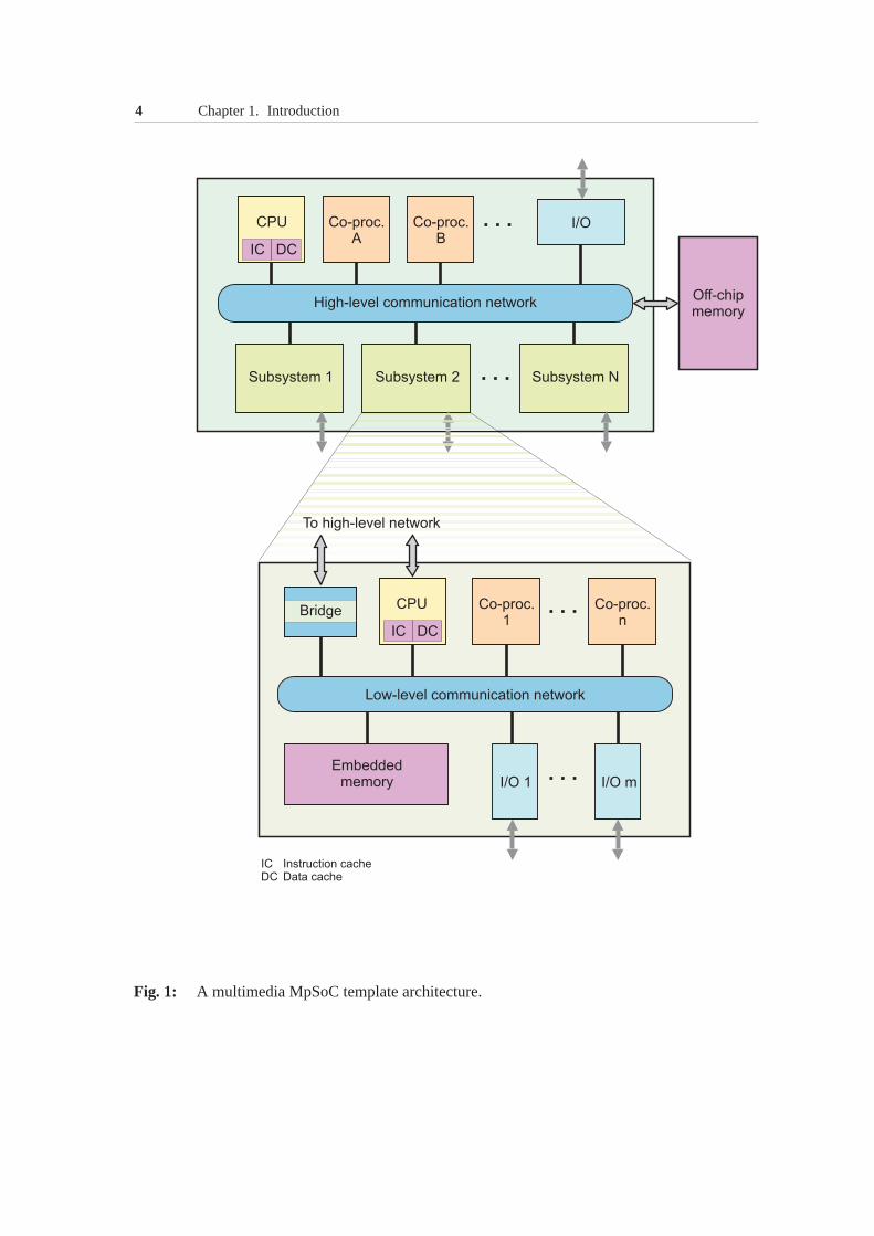
There are many examples of multimedia MpSoCs available from the indus-try and academy [38, 62, 63, 151, 155]. Most of them follow thedesign patternshown in Fig. 1: A typical multimedia MpSoC contains a numberof softwareprogrammable processors (CPUs, DSPs, media processors, etc.), weakly pro-grammable co-processors, fixed-function hardware modules, and peripheral de-vices (e.g. video and audio I/O blocks). These coarse-graincomputational com-ponents are interconnected by an on-chip communication network which mayencompass various types of busses, bridges, direct memory access (DMA) con-trollers, distributed memories, and other communication components. Followingthe emergingnetwork-on-chip(NoC) paradigm [31, 79], the on-chip communi-cation infrastructure may resemble a large-scale computernetwork, involvingsuch concepts as routers, switches, protocols, communication queues, etc.
The on-chip communication network may have a complex architecture con-sisting of several subnetworks interconnected by bridges,as shown in Fig. 1. Asubnetwork (low-level network) combines intensively communicating computa-tional components into a tight cluster (subsystem). In thisway, the local commu-nication traffic between the components within a subsystem is isolated from thesystem-wide data exchange taking place via a high-level on-chip network. Be-sides supporting the system-wide communication, this high-level network pro-vides an arbitrated access to a relatively large amount of inexpensiveoff-chip
4 Chapter 1. Introduction
Fig. 1: A multimedia MpSoC template architecture.
1.2. System-Level Design Issues 5
memory. This memory is primarily devoted for storing global data structures aswell as large data sets (e.g. full video frames) not fitting into smallerembeddedmemorieslocated on the chip. The on-chip memory is typically more expensivebut faster than the off-chip memory. Distributed around thearchitecture, the em-bedded memories store frequently accessed program code anddata structures.They are also used to implement performance-critical data exchange betweenthe on-chip computational components. To communicate certain data types, thecomponents may need to bypass the bridges interconnecting different subnet-works. For this, the components may be connected to more thanone subnetworkor directly to each other, thereby resulting in an irregularapplication-specificcommunication architecture.
1.1.2 System-level view of media processing
At the system level, a multimedia application executing on aheterogeneous mul-tiprocessor architecture, such as a multimedia MpSoC, can beviewed as a setof tasks (or processes) concurrently running on different execution resources ofthe architecture. These tasks communicate with each other solely throughuni-directional data streams[134, 135]. Each stream is sent from a producer task tothe corresponding consumer task through a first-in-first-out (FIFO) buffer. Thebuffer allows forasynchronous communicationbetween the tasks, thereby lead-ing to reduced communication overheads and increased utilization of the execu-tion resources [95]. Within the architecture, the buffers are allocated in sharedmemories or instantiated as dedicated hardware FIFO memoryblocks.
1.2 System-Level Design IssuesAlthough the integrated circuit technology provides greatopportunities for man-ufacturing increasingly complex MpSoCs, optimally designing such systems un-der high time-to-market pressures becomes more and more difficult. The grow-ing complexity of MpSoCs poses many challenges to their system-level design.Currently, there is a lack of methods and tools that could helpsystem designersto effectively tackle this complexity. A comprehensive discussion of the system-level design issues can be found elsewhere [72]. This section concentrates onlyon few of them relevant to the workload modeling problem addressed in this the-sis.
The goal of embedded system designers is to construct system’s architec-ture out of a set of hardware and software components. Due to alarge numberof such components and their heterogeneity, integrating them into a consistentworking whole (such as an MpSoC) represents an excessive design effort. Well-defined (and standardized) component interfaces and protocols can significantly
6 Chapter 1. Introduction
reduce this effort [72]. Although they may easy the task of building a function-ally correct system, they cannot help inverifying whether the resulting systemarchitecture meets performance requirements of the targetapplications.
Platform-based designfurther reduces the system design complexity by pro-viding a generic, domain-specific template architecture that only needs to becustomized for the target application range. Examples of such platforms inthe multimedia domain include OMAP from Texas Instruments [53], Nomadikfrom STMicroelectronics [6] and Nexperia [38] from Philips. The platformcustomization involves tuning various parameters of the template architecture,such as bus widths, memory sizes, cache configurations, clock rates of proces-sor cores,etc.; selecting and configuring resource management policies; and,possibly, adding to the basic architecture some application-specific components(e.g. co-processors), with the aim of obtaining an architecture that represents adesirable tradeoff between performance, energy consumption and cost.
Already for systems of moderate complexity, the resulting design space formedby all possible platform configurations may be huge and highly irregular. To effi-ciently explore this space, system architects must be able to quickly evaluate theperformance of candidate architectures. The performance evaluation has to pre-dict with a sufficient accuracy such characteristics of the prospective system asthroughput, memory requirements, utilization of execution resources, process-ing delays,etc. It should also help system designers to identify performancebottlenecks within the system.
Nowadays the mainstream in system-level performance evaluation of com-plex real-time embedded systems relies on simulation. Although simulationmay return very accurate performance estimations, its coverage is limited onlyto those workload instances that have been simulated. Hence, achieving a goodcoverage necessitates multiple simulation runs using carefully chosenrepresen-tative workload scenarios. In addition, accurate simulators oftentimes exhibithigh running times making them poorly suitable for a fast design space explo-ration cycle.
Irrespective of how many and which workload scenarios have been simu-lated, the simulation can never achieve, in a reasonable time, the full coveragerequired for theperformance verification. Because of this, it may not be used, forexample, to verify whether an embedded system satisfies the imposed on it tim-ing constraints in all possible workload scenarios. Such a verification is possibleusing formal analytic approaches that performworst-case performance analysis,i.e. return worst-case performance bounds.
The worst-case performance analysis uses aperformance modelwhich repre-sents an abstraction encompassing all system’s states and behaviors and all pos-sible workload scenarios. The performance analysis can therefore provide thefull coverage needed for the performance verification. Moreover, it is typicallyfaster than the simulation. However, due to the complexity of both the analyzedarchitectures and their workloads, it is extremely difficult to find proper sys-
1.2. System-Level Design Issues 7
tem abstractions that would lead to accurate (i.e. tight) worst-case performancebounds. This explains why in many design contexts, embeddedsystem engineersprefer to use simulation for the performance evaluation, inspite of its drawbacks.
1.2.1 Issues in design of multimedia MpSoCs
The performance evaluation issues discussed so far arise invarious system-leveldesign contexts and are not pertinent exclusively to the domain of multimediaMpSoCs. The discussion in this subsection concentrates on the design issuesthat are more specific to this domain.
Users expect from the media devices a high-quality and stable delivery of amultimedia content, and these expectations are growing fast. A central concernin the design of multimedia MpSoCs is therefore to ensure a specified quality ofservice(QoS) to the processed media streams. If a device has committed to pro-vide a certain QoS level, it has to guarantee this level underany circumstances.This requirement is especially difficult to fulfill because many multimedia appli-cations imposehighly variable and unpredictable workloadson the underlyingarchitectures [14, 57, 142, 165]. The designers of multimedia MpSoCs thereforeface a challenging problem of designing architectures capable of providing apredictable performanceunder uncertain workload conditions and stringent costand energy constraints.
The quality of media streams processed on an MpSoC depends ontwo fac-tors:
• First, as mentioned in Section 1.1, a violation of thetiming constraintsassociatedwith the stream processing may seriously impair the qualityof media streams.
• Second, the quality may also degrade if the FIFO buffers between the applicationtasks executing on the MpSoC experienceoverflows or underflows. This leadsto the concept ofbuffer constraints: An overflow (underflow) buffer constraintrequires that the corresponding buffer never overflows (underflows).
Hence, the QoS guarantees are specified in terms of the timingand buffer con-straints.
To provide the QoS guarantees under uncertain workload conditions, the re-sources of an embedded architecture for media processing have to be dimen-sioned for theworst-case workload. However, since the worst-case workloadoccurs rarely, the resources may remain underutilized mostof the time. A wayto improve the utilization is to share the resources among several independentconcurrent applications (or application tasks). Such a sharing has to respect theQoS guarantees associated with the processed media streams. This necessitatesdeployment of sophisticatedresource management policies. These policies mustbe able to satisfy timing and buffer constraints associatedwith several concur-rent streams imposing varying resource demands on the shared communicationand computational components of the architecture. Whereas the current practice
8 Chapter 1. Introduction
relies on computationally expensive dynamic schemes [135,137], the goal is todesign low-overhead resource management policies.
A major design effort is directed towards making embedded systems energy-efficient. This issue is crucial in the design of battery-operated multimedia de-vices, such as portable media players or cell phones. Achieving the energy effi-ciency requires multimedia MpSoCs to be adaptable to changing workload con-ditions. For this, the architectures provide various energy-saving mechanisms,e.g., support a variety of power modes. Intelligentrun-time adaptation strate-giesare needed to control these mechanisms. For instance, to reduce the energydissipated on an MpSoC component, the operating frequency and voltage of thiscomponent can be dynamically adjusted in response to workload fluctuations ex-perienced by it. Such a run-time energy management must be performed withoutjeopardizing the QoS guarantees associated with the media streams processed bythis component. This implies that the run-time adaptation strategies must be ableto handle the worst-case workload, which may occur sporadically.
1.3 The Workload Modeling ProblemEffectively addressing the system-level design issues outlined in the precedingsection requires a proper workload model:
• The selection of representative workload for an effective simulation-based per-formance evaluation necessitates a comparison of different workload scenarios.For the comparison, the workload scenarios have to be characterized based on amodel which captures interesting for the performance evaluation workload prop-erties. For example, if designers intend to determine by thesimulation the re-quired FIFO buffer sizes, they may want to identify a diverseset of workloadscenarios which produce maximum backlogs in different FIFObuffers of thearchitecture. Thus, the model they use for the workload characterization mayinclude such a property as burstiness of the communication patterns betweenapplication tasks.
• A workload model also forms the basis of any analytic performance model. It istherefore responsible for tightness of the worst-case bounds returned by the per-formance analysis. Tighter bounds imply less pessimism in the resource dimen-sioning, thereby leading to lower system cost and energy consumption. Hence,having a workload model which provides a pessimistic butaccurateworkloadcharacterization is essential in this context. Additionally, a successful workloadmodel should allow for an efficient analysis.
• Finally, a workload model is necessary in design of the resource managementpolicies and the energy-saving run-time adaptation strategies. These techniqueshave to be aware of the workload dynamics. This implies that these dynamics
1.3. The Workload Modeling Problem 9
(a)
0 0.2 0.4 0.6 0.8 1 1.2 1.4 1.6 1.8 20
2
4
6
8
macroblock index [×104]
exec
utio
n re
quire
men
t[p
roce
ssor
cyc
les
× 10
4 ]
(b)
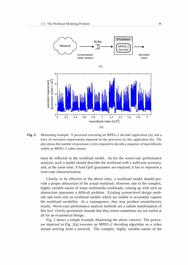
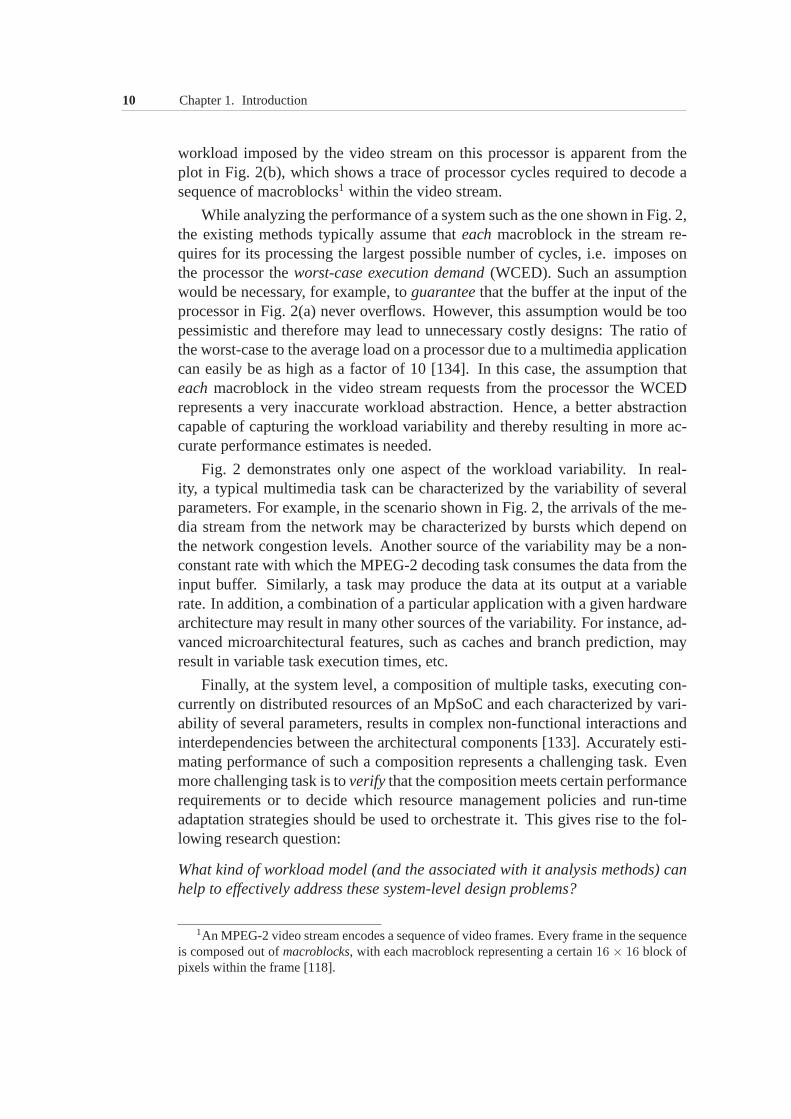
Fig. 2: Motivating example: A processor executing an MPEG-2 decoder application (a); and atrace of execution requirements imposed on the processor by this application(b). Theplot shows the number of processor cycles required to decode a sequence of macroblockswithin an MPEG-2 video stream.
must be reflected in the workload model. As for the worst-caseperformanceanalysis, such a model should describe the workload with a sufficient accuracy,and, at the same time, if hard QoS guarantees are required, ithas to represent awort-case characterization.
Clearly, to be effective in the above roles, a workload model should pro-vide a proper abstraction of the actual workload. However, due to the complex,highly variable nature of many multimedia workloads, coming up with such anabstraction represents a difficult problem. Existing system-level design meth-ods and tools rely on workload models which are unable to accurately capturethe workload variability. As a consequence, they may produce unsatisfactoryresults. Worst-case performance analysis methods are a salient manifestation ofthis fact: Overly pessimistic bounds that they return sometimes are not useful atall for an economical design.
Fig. 2 shows a simple example illustrating the above concern: The proces-sor depicted in Fig. 2(a) executes an MPEG-2 decoding algorithm on a videostream arriving from a network. The complex, highly variable nature of the
10 Chapter 1. Introduction
workload imposed by the video stream on this processor is apparent from theplot in Fig. 2(b), which shows a trace of processor cycles required to decode asequence of macroblocks1 within the video stream.
While analyzing the performance of a system such as the one shown in Fig. 2,the existing methods typically assume thateachmacroblock in the stream re-quires for its processing the largest possible number of cycles, i.e. imposes onthe processor theworst-case execution demand(WCED). Such an assumptionwould be necessary, for example, toguaranteethat the buffer at the input of theprocessor in Fig. 2(a) never overflows. However, this assumption would be toopessimistic and therefore may lead to unnecessary costly designs: The ratio ofthe worst-case to the average load on a processor due to a multimedia applicationcan easily be as high as a factor of 10 [134]. In this case, the assumption thateachmacroblock in the video stream requests from the processor the WCEDrepresents a very inaccurate workload abstraction. Hence,a better abstractioncapable of capturing the workload variability and thereby resulting in more ac-curate performance estimates is needed.
Fig. 2 demonstrates only one aspect of the workload variability. In real-ity, a typical multimedia task can be characterized by the variability of severalparameters. For example, in the scenario shown in Fig. 2, thearrivals of the me-dia stream from the network may be characterized by bursts which depend onthe network congestion levels. Another source of the variability may be a non-constant rate with which the MPEG-2 decoding task consumes the data from theinput buffer. Similarly, a task may produce the data at its output at a variablerate. In addition, a combination of a particular application with a given hardwarearchitecture may result in many other sources of the variability. For instance, ad-vanced microarchitectural features, such as caches and branch prediction, mayresult in variable task execution times, etc.
Finally, at the system level, a composition of multiple tasks, executing con-currently on distributed resources of an MpSoC and each characterized by vari-ability of several parameters, results in complex non-functional interactions andinterdependencies between the architectural components [133]. Accurately esti-mating performance of such a composition represents a challenging task. Evenmore challenging task is toverify that the composition meets certain performancerequirements or to decide which resource management policies and run-timeadaptation strategies should be used to orchestrate it. This gives rise to the fol-lowing research question:
What kind of workload model (and the associated with it analysis methods) canhelp to effectively address these system-level design problems?
1An MPEG-2 video stream encodes a sequence of video frames. Every frame in the sequenceis composed out ofmacroblocks, with each macroblock representing a certain16 × 16 block ofpixels within the frame [118].
1.4. Thesis Contributions 11
1.4 Thesis ContributionsIn this thesis, we propose a new model for characterization of multimedia work-loads in the system-level design of heterogeneous multiprocessor embedded com-puters. This workload model allows to effectively address many of the designissues described in the preceding sections. In particular,this thesis makes thefollowing main contributions:
• We introduce the concept ofVariability Characterization Curves(VCCs) as ameans to characterize entire classes of increasing functions or sequences basedon their worst-case and best-case variability. We then define several VCC typesfor the multimedia workload characterization (collectively referred to asmulti-media VCCs).
• We extend the modeling capabilities of theModular Performance Analysisframe-work [159, 160] and its mathematical foundation, theReal-Time Calculus[24,121, 157, 158], with the multimedia VCCs. Towards this, we introduce the con-cept ofworkload transformations, which enable anaccurate and efficientperfor-mance analysis of heterogeneous multiprocessor embedded systems under vari-able multimedia workloads. The extended analysis framework can return signif-icantly tighter performance bounds than those achievable without the workloadtransformations.
• We formulate the problem ofscheduling bursty media streams under strict bufferconstraintsand propose methods to address this problem. In particular,wepresenta framework for design of resource management policiesfor multimediaMpSoCs. The framework provides methods to quickly evaluate the quality andcheck the feasibility of various resource management policies to be deployedin an MpSoC. It fully relies on the VCC-based characterization of the mediastreams.
• We show how the VCC-based workload model can be used forenergy-efficientmedia stream processing. Towards this, we develop a run-time processor rateadaptation strategy which can be used in conjunction with the dynamic voltagescaling to achieve considerable energy savings while processing bursty multime-dia workloads under strict buffer constraints. In comparison to other methodsaddressing similar problems, our scheme handles multimedia workloads char-acterized by both, the data-dependent variability in the execution time of mul-timedia tasks and the burstiness in the on-chip traffic arising out of multimediaprocessing, and at the same time it provides hard QoS guarantees.
• We introduce the problem ofselecting representative workloadfor system-levelperformance evaluation of MpSoCs and propose a solution to this problem forthe case of multimedia workloads. Our method employs VCCs for the work-load characterization and supportsautomatic identification of the representativeworkload.

12 Chapter 1. Introduction
• Finally, we demonstrate the utility and experimentally assess the quality of theVCC-based workload model through several case studies involving realistic ap-plication scenarios. In the experiments, we compare our model with the existinganalytic approaches and with a detailed (transaction-level) system simulator.
1.5 Thesis Overview• The main purpose of Chapter 2 is to introduce the MPA frameworkwhose mod-
eling capabilities we extend in Chapter 3.
• Chapter 3 introduces the concepts of VCCs and workload transformations, de-fines the multimedia VCC types and proposes several workload transforma-tions based on them. This chapter also discusses possible ways to obtain VCCsand presents results of an experimental evaluation of the VCC-based workloadmodel.
• In Chapter 4, we address the problem of selecting representative workload forsystem-level performance evaluation of MpSoCs. We show how the VCC-basedworkload characterization model can be used for quantitative comparison andclassification of media streams and present results of an empirical validation ofthe proposed method.
• Chapter 5 introduces the problem of stream scheduling under buffer constraintsand presents the framework for design of resource management policies for mul-timedia MpSoCs. It focuses mainly on the methods for quick feasibility tests ofstream schedulers and estimation of buffer memory requirements resulting fromdeploying these schedulers on the processing elements of anMpSoC.
• Chapter 6 presents the VCC-based run-time processor rate adaptation techniquefor energy-efficient media stream processing under buffer constraints.
• Finally, Chapter 7 summarizes main results of this work.
2System-Level Performance Analysis
System-level performance analysis plays a key role in the design of complex em-bedded systems. It is used early in the design cycle to estimate characteristicsof the prospective embedded system and based on this estimation make criticaldesign decisions. The quality of these decisions thereforelargely depends on thequality of the estimates obtained from the performance analysis. This explainswhy a significant research effort is being invested in devising efficient perfor-mance analysis methods capable of producing accurate and reliable estimates ofthe system performance.
This chapter introduces the problem of system-level performance analysisof heterogeneous multiprocessor embedded systems. It briefly outlines existingapproaches to solving this problem and treats in detail one of them — the Mod-ular Performance Analysis (MPA) framework based on the Real-Time Calculus(RTC). This framework provides powerful abstractions and mathematical sup-port for a compositional performance analysis of distributed embedded systems.However, the basic abstractions it offers are not sufficientfor an accurate per-formance modeling of heterogeneous multiprocessor embedded computers formedia processing. We will address this problem in the next chapter by extendingthe modeling capabilities of the MPA framework.
14 Chapter 2. System-Level Performance Analysis
2.1 Introduction
2.1.1 Requirements
Early in the design cycle, embedded system designers face the problem of eval-uating many candidate hardware-software architectures with respect to variousperformance indexes. These indexes may include system’s throughput, responsetimes, end-to-end delays, resource utilization, memory requirements, etc. Inmost cases, building a prototype for each design alternative to directly measurethese performance characteristics is infeasible because of high implementationcosts and stringent time-to-market constraints. On the other hand, due to theincreasing complexity of modern embedded systems, back-of-the-envelope esti-mations cannot be used without taking the risk of being totally incorrect. Hence,the only option left for the designers is to carry out the performance analysisbased on some kind of aperformance modelof the system. This can be a simu-lator or a mathematical model. In any case, it should return sufficiently accurateestimates of the system performance. Furthermore, to allowfor a fast designspace exploration, the performance model should also be efficiently analyzableand easily constructible. The latter property is especially important for support-ing automated design space exploration.
Designing embedded systems that must satisfy real-time constraints faces ad-ditional challenges associated with the need toverify timing correctness of theirbehavior. For instance, it might be necessary to verify whether the time elapsedbetween two specified events within the systemeverexceeds a given value. Sucha verification can only be accomplished using a formal systemmodel support-ing worst-case analysis, which implies a complete coverageof all possible statesof the system and of its environment. Neither system’s prototype nor its simu-lator can be employed for the performance verification purposes as (due to thehigh system complexity) it is hardly possible to check all system states within areasonable time frame.
2.1.2 Input specification
A starting point for the system-level performance analysisis a specificationwhich typically describes the following aspects of an embedded system:
• Application task structureThe application task structure is typically modeled by atask graph(or a set oftask graphs) that captures a partitioning of the target application into individ-ual tasks, and models data and control dependencies betweenthem. Interactionsbetween the tasks in a task graph may be governed by a specificmodel of com-putation. For example, multimedia applications are often modeled using the for-malism ofKahn Process Networks[70, 134, 135], which assumes that the taskscommunicate via FIFO channels.
2.1. Introduction 15
• Task assignment to processing elementsThe application tasks performing data transformations areassigned for executionto computational resourcessuch as CPUs, DSPs and co-processors, while thetasks responsible for data transfers are assigned tocommunication resourcessuchas busses, DMA controllers, bridges, etc. Throughout this thesis we refer toboth resource types asprocessing elements(PEs) because in principle for theperformance analysis it is irrelevant whether an architectural resource executescomputation or communication tasks.
• Resource management policiesAs a result of the task assignment, multiple tasks may be mapped on to one PE.In this case, a scheduling (or arbitration) policy is deployed to manage tasks’access to this PE. In general, several different schedulingand arbitration policiesmay be deployed within the architecture.
• Storage resource allocationData arrays manipulated by the tasks, for example, the buffers implementing theFIFO communication channels, are assigned to the off- and on-chip memories.
• Characteristics of processing elementsFor the performance analysis we need to specify capabilities of processing el-ements. Therefore, such parameters as clock rates of processors and effectivecommunication bandwidths of busses typically form a part ofthe input specifi-cation.
• Task propertiesThese include a variety of relevant to the performance analysis task characteris-tics, for example, the number of processor cycles needed to complete a task on agiven PE and the size of data items to be exchanged between thetasks.
• Characteristics of the environmentThe input specification should also capture characteristics of the event streams tobe processed by the embedded system. These characteristicsmay include timingproperties of the event streams (e.g. their arrival rates) as well as their possiblecontents, for example, different event types that may appear in a given event flow.
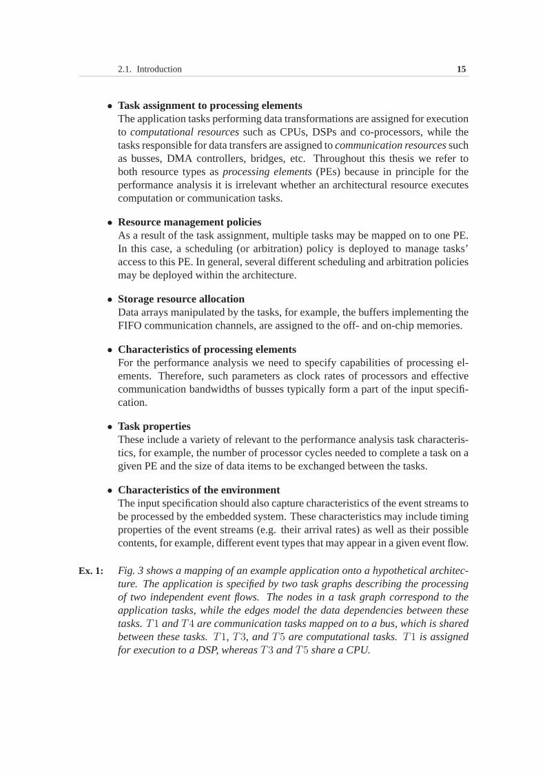
Ex. 1: Fig. 3 shows a mapping of an example application onto a hypothetical architec-ture. The application is specified by two task graphs describing the processingof two independent event flows. The nodes in a task graph correspond to theapplication tasks, while the edges model the data dependencies between thesetasks.T1 andT4 are communication tasks mapped on to a bus, which is sharedbetween these tasks.T1, T3, andT5 are computational tasks.T1 is assignedfor execution to a DSP, whereasT3 andT5 share a CPU.
16 Chapter 2. System-Level Performance Analysis
Fig. 3: An example application-to-architecture mapping.
2.1.3 Existing approaches to performance analysis
Based on the kind of specification described in the previous subsection, design-ers need to build a performance model of the system. They can do this in severalways. For example, they could construct a system simulator [15], use a trace-based performance evaluation technique [83, 125], create astochastic model ofthe system [93] or employ a worst-case performance analysismethod. Theirchoice depends on the analysis goals (and on the available expertise and tools).A comparative overview of various approaches to the performance analysis ofembedded systems can be found elsewhere (see, e.g. [159]). In this chapter, weconcentrate on techniques suitable for theperformance verification, i.e. on theworst-case performance analysis methods. Furthermore, here we limit the dis-cussion only to those methods that can be applied to distributed (multiprocessor)embedded systems having heterogeneous hardware-softwarearchitectures. Bytheheterogeneitywe mean not only the diversity of processing elements makingup the architecture but also the variety of scheduling and arbitration policies thatmight be deployed on those processing elements.
The need to ensure the timing correctness ofdistributed real-time embed-ded systems has led to the development of methods that can analyze worst-caseend-to-end response times of entire task chains mapped ontomultiple processornodes communicating via a shared bus. Such methods have beentermedholis-tic scheduling analysisbecause they tightly integrate the schedulability analysisof individual processing elements (i.e. processors and communication channels)into an overall piece of analysis [163]. The first holistic method proposed inTindell et al. [163] addressed systems with fixed priority scheduling policy de-ployed on processor nodes communicating via a bus using a time division multi-ple access (TDMA) protocol. Later many extensions and generalizations of thismethod appeared in the literature (see, e.g. [48, 128, 130] and references therein).
2.2. Modular Performance Analysis 17
These methods can be very effective in modeling complex timing relations (e.g.phasing) between the tasks. However, they are often attributed a lack of scalabil-ity and modularity [68, 159], which are needed for modeling large heterogeneoussystems (perhaps, with hundreds of nodes) and for quick modifications of theseperformance models during a design space exploration cycle. In other words,these techniques might need to be redesigned for each new system configura-tion.
The above problem has been partially addressed in Ernstet al. [68, 133].Their approach advocates acompositional performance analysismethodologywhich uses propagation of abstract event streams between various schedulinganalysis techniques locally applied to the processing elements (components).The basic idea is to reuse existing (standard) scheduling techniques for the lo-cal analysis. This entails using standard event models (e.g. sporadic, periodic,periodic with jitter, periodic with bursts) and adapting them between the com-ponents which use incompatible event models. These adaptations as well as thestandard event models themselves may be overly pessimistic, leading to a loss inaccuracy. Furthermore, since the method heavily relies on the existing schedul-ing analysis techniques, supporting any new (not yet existing) scheduling policynecessitates devising an analysis for it; i.e. essentiallythe method suffers fromthe same problem as the holistic scheduling analysis discussed above.
In the next section, we describe the MPA framework [159, 160], which triesto overcome the drawbacks of other scheduling analysis methods by following acompletely different approach to the performance analysis, which does not relyneither on the standard event models nor on the traditional scheduling analysismethods, while offering a high degree of generality and modularity.
2.2 Modular Performance Analysis
2.2.1 Basic idea
In essence, any performance analysis involves two basic concepts — theservicerequestedby an application (task) and theservice offeredby the architecture tothis application (task). Temporal interactions between the requested and the of-fered service determine performance characteristics of the system. The ultimategoal of any performance analysis method is therefore to properly capture theseinteractions. In this subsection, we describe how this is achieved in the MPAframework.
The basic idea behind the MPA framework is to model the interactions be-tween the requested and the offered service using the concept of scheduling net-work. In a scheduling network, the requested and the offered service are modeledby event and resource streams. These streams flow through the network nodes,
18 Chapter 2. System-Level Performance Analysis
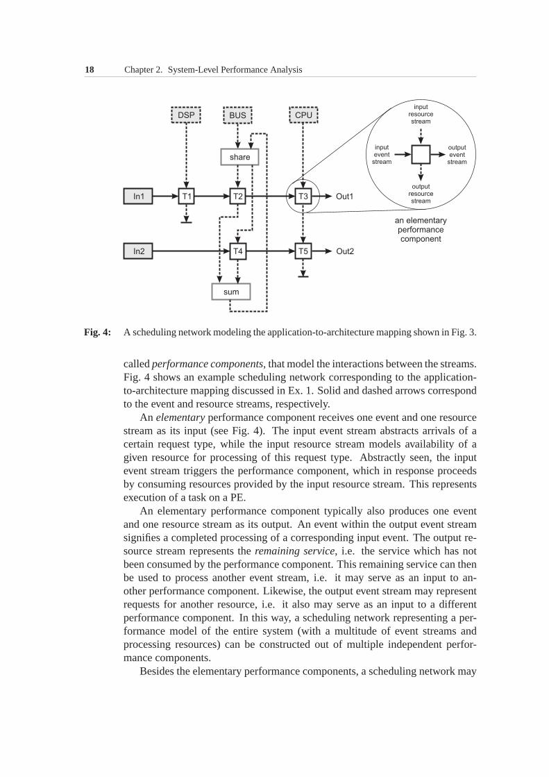
Fig. 4: A scheduling network modeling the application-to-architecture mapping shownin Fig. 3.
calledperformance components, that model the interactions between the streams.Fig. 4 shows an example scheduling network corresponding tothe application-to-architecture mapping discussed in Ex. 1. Solid and dashed arrows correspondto the event and resource streams, respectively.
An elementaryperformance component receives one event and one resourcestream as its input (see Fig. 4). The input event stream abstracts arrivals of acertain request type, while the input resource stream models availability of agiven resource for processing of this request type. Abstractly seen, the inputevent stream triggers the performance component, which in response proceedsby consuming resources provided by the input resource stream. This representsexecution of a task on a PE.
An elementary performance component typically also produces one eventand one resource stream as its output. An event within the output event streamsignifies a completed processing of a corresponding input event. The output re-source stream represents theremaining service, i.e. the service which has notbeen consumed by the performance component. This remainingservice can thenbe used to process another event stream, i.e. it may serve as an input to an-other performance component. Likewise, the output event stream may representrequests for another resource, i.e. it also may serve as an input to a differentperformance component. In this way, a scheduling network representing a per-formance model of the entire system (with a multitude of event streams andprocessing resources) can be constructed out of multiple independent perfor-mance components.
Besides the elementary performance components, a scheduling network may
2.2. Modular Performance Analysis 19
contain other types of nodes:
• Resource modulesmodel processing capabilities of PEs within the architecture.A resource module produces a stream corresponding to theunloadedresourcethat it models. In Fig. 4, resource modules are marked with dashed boxes. Theyrepresent the bus, DSP and CPU resources from Ex. 1.
• Input modules inject into the scheduling network event streams generatedbythe system’s environment. In Fig. 4, these areIn1 andIn2 modules.
• Scheduling modulesdistribute resource streams between different performancecomponents in accordance with a given resource management policy. A schedul-ing module receives and produces only resource streams (originated by the sameresource). Using scheduling modules we can model differentscheduling and ar-bitration policies deployed on the PEs of the architecture.In Fig. 4, for example,we haveshare andsum scheduling modules.
• Hierarchical modules are complex performance components containing sub-networks of other components.
For the performance analysis, in addition to thestructuralperformance viewof the system provided by the scheduling network, we need also to characterizebehaviorof the event and resource streams, and of the associated performancecomponents. That is we need to characterize timing properties of the streamsand determine how these properties change when the streams pass through theperformance components in the scheduling network. This canbe done in manydifferent ways. For example, we could simply simulate the scheduling networkusing appropriate event traces. However, our objective is amethod which can beused for the worst-case performance analysis. To achieve this objective, we canrely on the mathematical foundation provided by the Real-Time Calculus, whichis briefly introduced in the next section.
2.2.2 Real-Time Calculus
The Real-Time Calculus [24, 121, 157, 158] provides powerful abstractions ofthe event and resource streams and uses these abstractions to mathematicallymodel the behavior of an elementary performance component.This basic modelcan then be used for a component-wise evaluation of a whole scheduling net-work. In addition, the Real-Time Calculus allows to compute various perfor-mance indexes of the system, such as upper bounds on the delayand backlogexperienced by the events while being processed in the system.
Characterization of event and resource streamsTiming properties of event and resource streams are captured usingarrival andservice curves.
20 Chapter 2. System-Level Performance Analysis
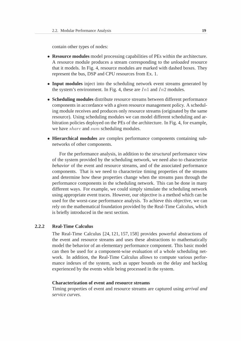
Fig. 5: Modeling periodic event streams with jitter using arrival curves.
An event stream is abstracted by a pair of arrival curves,αu(∆) andαl(∆),which give respectively upper and lower bounds on the numberof events seen inthe event stream within any time interval of length∆.
A resource stream is modeled by a pair of service curves,βu(∆) andβl(∆),which give respectively upper and lower bounds on the resource amount (e.g.number of processor cycles) offered within any time interval of length∆.
The arrival and service curves can accurately describe streams with arbitrarycomplex timing behavior. On the other hand, a single pair of upper and lowercurves can capture an entire class of streams with similar timing properties. Forexample, many standard event models (e.g. sporadic, periodic, periodic withjitter, periodic with bursts) can be represented by the arrival curves [24]. Fig. 5illustrates this fact by showing how the arrival curves model a class of periodicevent streams with jitter.
Scheduling network evaluationThe performance analysis using the MPA approach entails a scheduling networkevaluation. The evaluation can be accomplished component-wise, by propagat-ing the event and resource streams through the network. Doing this requires amodel describing how the timing properties of the event and resource streams getchanged as a result of passing through the performance components. Since eventand resource streams are abstracted by the arrival and service curves, we needa mathematical model describing how an elementary performance componenttransforms the shapes of these curves. Such a model, provided by the Real-TimeCalculus, is given by the following set of equations [24]:
αuO = [(αu
I ⊗ βuI )⊘ βl
I ] ∧ βuI (2.1)
αlO = [(αl
I ⊘ βuI )⊗ βl
I ] ∧ βlI (2.2)
βuO = (βu
I − αlI)⊘ 0 (2.3)
βlO = (βl
I − αuI )⊗ 0 (2.4)
αuI , αl
I , βuI and βl
I denote the arrival and the service curves characterizing theevent and the resource streams at the input of an elementary performance com-ponent, respectively.αu
O, αlO, βu
O andβlO provide the corresponding characteri-
2.2. Modular Performance Analysis 21
zation of the streams at the output of the component. The model assumes thatthe events belonging to the same stream are processed in their arrival order andthat they are stored in a FIFO buffer while waiting to be served.
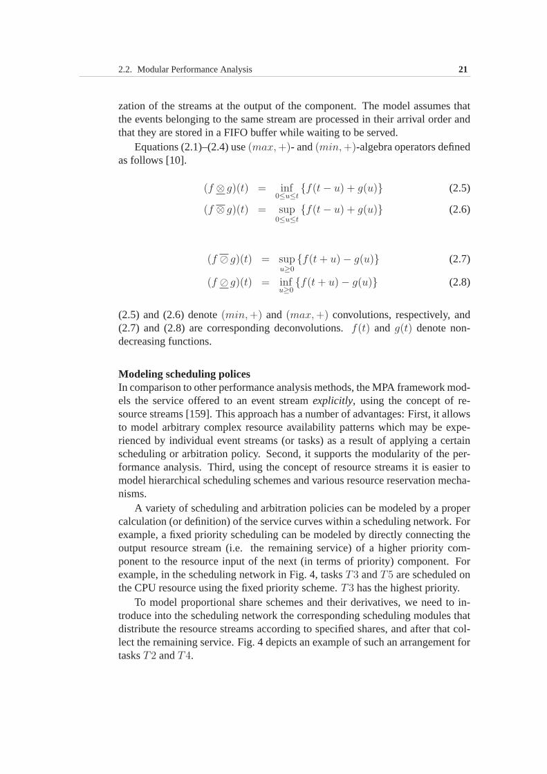
Equations (2.1)–(2.4) use(max,+)- and(min,+)-algebra operators definedas follows [10].
(f ⊗ g)(t) = inf0≤u≤t
{f(t− u) + g(u)} (2.5)
(f ⊗ g)(t) = sup0≤u≤t
{f(t− u) + g(u)} (2.6)
(f ⊘ g)(t) = supu≥0
{f(t+ u) − g(u)} (2.7)
(f ⊘ g)(t) = infu≥0
{f(t+ u) − g(u)} (2.8)
(2.5) and (2.6) denote(min,+) and (max,+) convolutions, respectively, and(2.7) and (2.8) are corresponding deconvolutions.f(t) and g(t) denote non-decreasing functions.
Modeling scheduling policesIn comparison to other performance analysis methods, the MPA framework mod-els the service offered to an event streamexplicitly, using the concept of re-source streams [159]. This approach has a number of advantages: First, it allowsto model arbitrary complex resource availability patternswhich may be expe-rienced by individual event streams (or tasks) as a result ofapplying a certainscheduling or arbitration policy. Second, it supports the modularity of the per-formance analysis. Third, using the concept of resource streams it is easier tomodel hierarchical scheduling schemes and various resource reservation mecha-nisms.
A variety of scheduling and arbitration policies can be modeled by a propercalculation (or definition) of the service curves within a scheduling network. Forexample, a fixed priority scheduling can be modeled by directly connecting theoutput resource stream (i.e. the remaining service) of a higher priority com-ponent to the resource input of the next (in terms of priority) component. Forexample, in the scheduling network in Fig. 4, tasksT3 andT5 are scheduled onthe CPU resource using the fixed priority scheme.T3 has the highest priority.
To model proportional share schemes and their derivatives,we need to in-troduce into the scheduling network the corresponding scheduling modules thatdistribute the resource streams according to specified shares, and after that col-lect the remaining service. Fig. 4 depicts an example of suchan arrangement fortasksT2 andT4.
22 Chapter 2. System-Level Performance Analysis
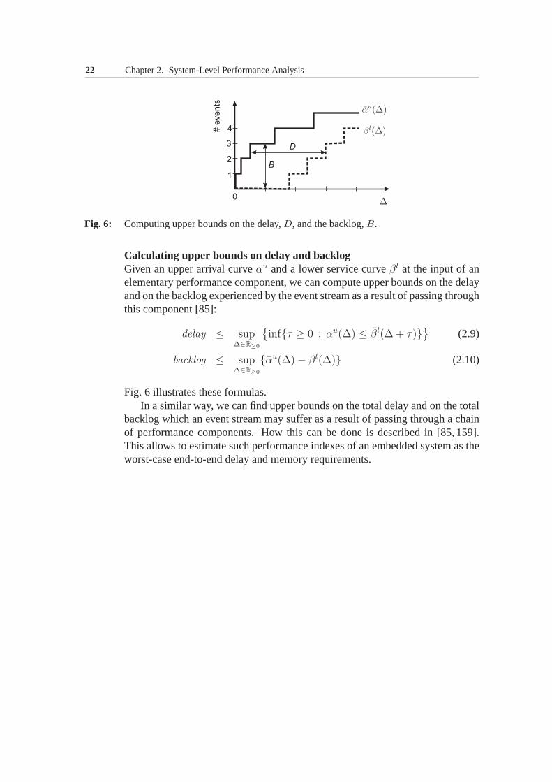
Fig. 6: Computing upper bounds on the delay,D, and the backlog,B.
Calculating upper bounds on delay and backlogGiven an upper arrival curveαu and a lower service curveβl at the input of anelementary performance component, we can compute upper bounds on the delayand on the backlog experienced by the event stream as a resultof passing throughthis component [85]:
delay ≤ sup∆∈R≥0
{
inf{τ ≥ 0 : αu(∆) ≤ βl(∆ + τ)}}
(2.9)
backlog ≤ sup∆∈R≥0
{αu(∆) − βl(∆)} (2.10)
Fig. 6 illustrates these formulas.In a similar way, we can find upper bounds on the total delay andon the total
backlog which an event stream may suffer as a result of passing through a chainof performance components. How this can be done is describedin [85, 159].This allows to estimate such performance indexes of an embedded system as theworst-case end-to-end delay and memory requirements.
3Modeling Variable Workload
This chapter introduces two central to this thesis concepts:
• Variability Characterization Curves (VCCs); and
• Workload Transformations.
VCCs allow to capture variability of different workload characteristics. Inthis chapter, we define several VCC types for modeling multimedia workloadsin the system-level design context of MpSoC architectures and describe variousways to obtain VCCs.
Tightly coupled with the concept of VCCs are the workload transformations.They extend the modeling capabilities of the RTC-based Modular PerformanceAnalysis (MPA) framework introduced in the previous chapter. This extensionpotentially leads to considerably tighter analytic performance bounds than thoseobtained using traditional workload models. This chapter provides a discus-sion on how the workload transformations can be optimally placed in an RTCscheduling network.
Towards the end of this chapter we present the results of an experimentalstudy comparing the proposed VCC-based workload model with a conventionalmodel. We also assess the quality of the VCC-based model using asystem sim-ulator. As a basis for the experimental study we consider twodesign problemsfrom the area of media processors and show how they can be solved using theVCC-based model. We thereby demonstrate first applications ofVCCs in thesystem-level design context of multimedia MpSoC architectures. Other applica-tions of VCCs in this context will be presented in the followingchapters.
24 Chapter 3. Modeling Variable Workload
Contributions of this chapter
• We introduce the concept of Variability Characterization Curves—a general modelfor compact representation of whole classes of increasing functions or sequencesbased on their worst-case and best-case variability.
• We propose and define VCC types for workload modeling of multimedia appli-cations mapped onto multiprocessor heterogeneous architectures.
• We extend the existing RTC-based MPA framework with workloadtransforma-tion operations which enable system-level performance analysis of heteroge-neous multiprocessor architectures under workloads characterized by variabilityof several parameters, such as task’s execution demands andI/O rates. We showhow such workload transformations can be optimally used in the analysis.
• Through experiments we evaluate the VCC-based workload model. We quantifythe gain from using this model by comparing it to a traditional task model widelyused in the literature. We also demonstrate utility and assess the accuracy of theVCC-based model using measurements obtained from a detailed system simula-tor. This experimental study gives important insights on the nature of MPEG-2video workloads and their characterization with VCCs.
Organization of this chapter
• Section 3.1 gives an overview of the related work
• Section 3.2 introduces the concept of VCCs and develops the necessary theoret-ical background.
• Section 3.3 reviews key properties of multimedia workloadsand on this basisdefines VCC types for multimedia workload modeling (multimedia VCCs).
• Section 3.4 introduces the concept of workload transformations and proposesseveral such transformations based on the multimedia VCCs defined in Sec-tion 3.3. Furthermore, this section discusses optimal placement of workloadtransformations in a RTC scheduling network.
• Section 3.5 elaborates on the ways to obtain VCCs.
• Section 3.6 presents results of the experimental evaluation of the VCC-basedmodel.
• Finally, Section 3.7 concludes the chapter.
3.1. Related Work 25
3.1 Related Work
This section outlines the existing approaches to model the workload for real-timescheduling and performance analysis of embedded systems.
Many results in the classical real-time scheduling theory [41, 150] are basedon the task model introduced in [100] by Liu and Layland. In this model, tasksare characterized by tuples(Ci, Ti), whereCi is execution time of taskτi andTi is the period with whichτi arrives into the system; tasks are assumed to beindependent and have deadlines equal to their periods. Subsequent research workmainly aimed at relaxing the assumptions about strict periodicity of task arrivalsand deadlines. For instance, [97] considers tasks with arbitrary deadlines, lessthan their periods, whereas in the model of [92] the deadlines are greater thanthe task periods. The model in [96] allows periodic tasks to arrive with fixedoffsets in time. In [162] tasks can have arbitrary deadlines, release jitter andbursty arrivals. Sporadic tasks are often modeled by constraining their minimuminter-arrival time [101].
To provide hard real-time guarantees workload models used in the classicalreal-time scheduling theory assume that every task instance requires WCET tocomplete. This assumption, although safe, is too pessimistic for a large classof applications characterized by high execution time variability; it may lead topoor processor utilization and, as a consequence, to designs with unreasonablyhigh cost or power consumption or both. Different approaches addressing thisproblem have been reported in the literature [140]. In the sequel we focus thediscussion on those approaches that further generalize theworkload model.
One important direction in modeling tasks characterized byvariable execu-tion demands and irregular arrivals is to usestochastic models. For example,task models in [7, 71, 109, 161] specify task execution demands using probabil-ity distributions and assume periodic arrivals. Methods in[7, 161] handle sets ofindependent tasks, while [71, 109] consider task sets with precedence relations.Real-Time Queuing Theory, first introduced in [93], uses stochastic character-ization for inter-arrival times, execution demands and deadlines, and relies onqueuing theoretic methods for performance evaluation. These and other stochas-tic workload models can result in tighter analytic bounds and hence in moreeconomical designs, but at the expense of some (usually controlled) fraction ofmissed deadlines. Because of this their application area is limited to soft real-timesystems only.
Another line of research work aims at reducing the pessimismof the clas-sical real-time task models by developing more expressive “deterministic” taskmodels suitable for the analysis ofhard real-timesystems. Mok and Chen [117]proposes amultiframe task model. As its basis this model has the classical pe-riodic task model of Liu and Layland [100]; however, it permits tasks whoseWCETs may vary from one instance to another. Such a task can be representedby a set of subtasks, each characterized by its own WCET. The subtasks in the
26 Chapter 3. Modeling Variable Workload
set are cyclically triggered in a predetermined order and with a time separationequal to the period of the task they represent. In [13] this multiframe model hasbeen extended to allow for the time separation between subtask activations to bealso variable (i.e. to cycle through a fixed pattern).
Baruah [11, 12] presents arecurring real-time task model(RRT)—a furthergeneralization of the multiframe models. In the RRT model, a task is modeledby a set of subtasks arranged in a directed acyclic graph representing the con-ditional, non-deterministic behavior of the task. Each subtask is characterizedby its WCET, a relative deadline and a minimum triggering separation from itsdirect predecessors. The whole task graph is triggered sporadically with a spec-ified minimum time separation between the triggering of the last subtask in thegraph and the triggering of the next task instance. Another workload model, alsousing conditional directed acyclic graphs to model tasks, is reported by Pop etal. in [127]. Instead of associating a deadline toeachsubtask in a task graph,the model in [127] associates a single deadline with the whole graph. Further-more, it exposes the parallelism within a task for mapping ona multiprocessorarchitecture.
In comparison to classical task models, the RRT model offers agreat flexi-bility in modeling variability of the execution demand and irregular inter-arrivaltimes. This flexibility is, however, limited torecurring patterns. If workloadbursts (characterized by periods with dense arrivals of tasks or increased execu-tion demand or both) occur relatively seldom, then avoidingoverly pessimisticresults under the RRT model necessitates to consider very large task graphs,leading to inefficiency of the analysis. In other words, designers have to tradeoff the accuracy of the analysis for the analysis time, whichfor the RRT modelincreases exponentially with the problem size [12].
Inspired by traffic characterization models in the domain ofcommunicationnetworks [85], an alternative workload model generalizingmany previous re-sults, including the RRT model, has been proposed by Thiele etal. [121, 158].The workload imposed by a task on a processor or a communication resource isabstracted by anarrival curvegiving the maximum amount ofresourceswhichcan be requested by the task within any time interval of a given length. In ad-dition, this model also captures the variability of the service offered to a task:a service curvegives the minimum amount of resources offered to a given taskon a resource within any time interval of a given length. The resulting work-load model can be efficiently analyzed using the mathematical framework ofReal-Time Calculus(RTC) [158], having its roots in the min-max algebra [10].As the RRT model, the arrival curves allow to capture arbitrary complex pat-terns of inter-arrival times and execution demands; however, in contrast to theRRT model, an accurate characterization of both short-term and long-term be-havior of the workload is achieved in a relatively compact form. Furthermore,the complexity of the analysis in general is not dependent onthe accuracy ofthe workload model, and efficient approximations can be doneif needed [156].
3.1. Related Work 27
Another important feature of the workload model presented in [121, 158] is thatunlike previous lines of work this model explicitly characterizes the service vari-ability, thereby allowing to effectively abstract arbitrary complex scheduling andarbitration policies deployed on communication and computational resources, aswell as such architectural features as caches, pipelines, write buffers, protocolsetc. Continuing this line of work, Chakraborty and Thiele [26]proposed a newtask model for streaming applications combining the concept of arrival curveswith the RRT model, which may help to reduce the size of task graphs of theRRT model while modeling complex event streams.
Most of the approaches discussed so far are not concerned with modellingtasks whichasynchronouslyinteract while processing event streams; meaningthat these approaches assume that a task producing an event (or a stream object)is never activated again before the dependent task consumesthis event (and fin-ishes its processing). Hence, these approaches are not interested in the propertiesof output event streams (activating the consumer tasks) andin variations of inputand output rates of tasks (i.e. in the number of events consumed or produced bya task per activation). However, these properties of the workload become impor-tant in context of distributed execution platforms for stream processing applica-tions. In this context different event streams may interacton shared resources,leading toscheduling anomalies: when a best-case load on one architecturalcomponent may cause a worst-case load scenario for another component [133].In this situation it becomes important to capture in the model not only worst-casebut also best-case behavior of the workload.
The importance of modeling both the worst-case and the best-case workloadbehavior in design context of embedded systems has been recognized in suchmodeling frameworks as SPI (System Property Intervals) [171, 182, 183]. Incontrast to the research work on real-time scheduling mentioned above, the SPIframework has a different focus: its prime goal is modeling of heterogeneous em-bedded systems for theirglobal performance analysis, design space exploration,optimization and synthesis. The SPI model represents a system as a network ofcommunicating processes which allows (besides other communication modes)the asynchronous communication via unidirectional FIFO channels. In the SPImodel each process is characterized by a set ofbehavioral intervalscapturingworst-case and best-case values of various process properties such as executiontime and the number of tokens consumed from input and produced to outputchannels. The SPI framework allows for refinement of this workload modelthrough the concept ofprocess modes. Following this concept, each process isassociated with a set of modes, each of which is characterized by its own setof the behavioral intervals. When the model is evaluated (e.g. executed), theprocess may change its modes depending on, for example, input values.
Through the concepts of behavioral intervals and process modes the SPIframework can model the workload with a high accuracy. However, this re-quires anexplicitspecification of conditions upon which the modes are changed,
28 Chapter 3. Modeling Variable Workload
and therefore significantly complicates the workload modeling process and maypreclude an efficient analyzability of the model. In fact, the SPI model offers aflexible tradeoff between the accuracy of the workload modeland the modelingoverhead: depending on the scenario a designer may decide how many differentmodes to associate with a process. In the simplest case, a process may have onlyone mode, as it is the case, for example, in [67] where the input (output) rate ofa process is specified with a single behavioral interval. This approach, however,results in overly pessimistic bounds and does not accurately capture the long-term behavior of the workload, which is important, for instance, in multimediaapplications.
Another framework for analysis of system properties proposed in [23, 24,157] is based on RTC developed in [121, 158]. In comparison tothe model usedin [121, 158], the workload model in [23, 24, 157] has a concept of lower andupperarrival and service curves which capture the best- and worst-case behaviorof the workload. In addition, [23, 24, 157] enhance the analytical framework in[121, 158] with mechanisms to determine properties of the output event streams.These developments pave the way to amodular approach to the performanceanalysis [159, 160]. However, the workload model in [23, 24,157] can modelonly tasks that consume and produce only one event per activation. Furthermore,for computing the output event streams it becomes necessaryto convert the ar-rival curves expressed in terms of event-based units into equivalents expressedin resource-based units and backwards. Since this conversion is performed byscaling the curves with a constant factor corresponding to WCED for process-ing of one event, the execution time variability is not accounted for, resulting inoverly pessimistic analytic bounds for workloads with large variations in execu-tion demand of tasks. These limitations of the framework have been addressedin [113, 115]. The results of [113, 115] are included in this chapter. Furtherrefinements of this workload model can be found in [166, 168, 169].
3.2 Variability Characterization Curves
This section defines Variability Characterization Curves (VCCs) in a genericway, i.e. without regard to any concrete system property that they character-ize. It also states some properties which are common to all VCCsand which willbe useful in the course of this thesis.
3.2.1 Definitions
Let A denote a set of increasing functionsAi, i = 1, 2, . . . andT denote thedomain of these functions, such thatAi : T → R≥0. T can be either theset of nonnegative real numbers (T = R≥0) or the set of nonnegative inte-

3.2. Variability Characterization Curves 29
gers (T = Z≥0).1 In the latter case, the functions inA represent sequences, i.e.Ai = 〈Ai(0), Ai(1), . . .〉. Formally, a functionf is increasingif f(x1) ≤ f(x2)for anyx1 < x2. In contrast,f is strictly increasingif f(x1) < f(x2) wheneverx1 < x2. Using this notation we define VCCs as follows.
Def. 1: (Upper VCC) An upper VCC for the set of increasing functionsA is an increas-ing functionVu
A satisfying the condition
Ai(t+ s) − Ai(t) ≤ VuA(s) ∀t, s ∈ T, ∀Ai ∈ A and Vu
A(0) = 0
Def. 2: (Lower VCC) A lower VCC for the set of increasing functionsA is an increasingfunctionV l
A satisfying the condition
Ai(t+ s) − Ai(t) ≥ V lA(s) ∀t, s ∈ T, ∀Ai ∈ A and V l
A(0) = 0
In caseT = R≥0 we adopt the convention that any upper VCC is a left-continuous function and any lower VCC is a right-continuous function. Notethat functionsAi are not required to conform to this convention. They can beeither left-continuous or right-continuous without restriction.
In caseT = Z≥0 the corresponding VCC is a sequence. If necessary a VCCwhich is a sequence can be converted into an equivalent VCC defined onR≥0.The conversion can be done by a continuation inT which respects the aboveconvention about continuity of VCCs. More specifically, letVu
AZ≥0
andV lAZ≥0
denote upper and lower VCCs defined onZ≥0. They can be converted into theircontinuous equivalentsVu
AR≥0
andV lAR≥0
as follows
VuAR≥0
(s) = VuAZ≥0
(⌈s/τ⌉) (3.1)
V lAR≥0
(s) = V lAZ≥0
(⌊s/τ⌋) (3.2)
whereτ denotes the desired spacing between samples ofVuAZ≥0
(or V lAZ≥0
) in
R≥0.A conversion in the opposite direction, i.e.VAZ≥0
→ VAR≥0
, is also possible:
VuAZ≥0
(k) = VuAR≥0
(kτ) k ∈ Z≥0 (3.3)
V lAZ≥0
(k) = V lAR≥0
(kτ) k ∈ Z≥0 (3.4)
Remark on notation: To simplify the notation, in some contexts we will skipsubscriptA in Vu
A and inV lA if it is irrelevant which function set is characterized
by the VCCs, i.e. we will simply writeVu andV l instead ofVuA andV l
A.
1Throughout this thesis, whenever we useT without specifying whetherT = R≥0 or T =Z≥0 we mean that both cases are possible, i.e.T is a placeholder forR≥0 andZ≥0.
30 Chapter 3. Modeling Variable Workload
From Defs. 1 and 2 it follows that a VCC is a mapping fromT to R≥0. Of-ten, however, while modeling systems with VCCs, there is a needfor the inversetransformation. Such a transformation could be possible via inverse functionsof VCCs. Unfortunately, since VCCs in general are not strictly increasing func-tions, they are not invertible in the conventional sense, i.e. for a given VCC theremay not exist a functionV−1 such thatV−1(V(t)) = t for all t. Therefore, weneed to introduce a notion ofpseudo-inverse functions.
Def. 3: (Pseudo-inverse of Upper VCC)The pseudo-inverse of an upper VCCVu is thefunction
Vu−1
(v) = sup{t : Vu(t) ≤ v; t ∈ T} (3.5)
Def. 4: (Pseudo-inverse of Lower VCC)The pseudo-inverse of a lower VCCV l is thefunction
V l−1
(v) = inf{t : V l(t) ≥ v; t ∈ T} (3.6)
3.2.2 Properties
Several useful properties of VCCs follow from the definitions given in Sec-tion 3.2.1.
Prop. 1: (Pseudo-inversion of Upper VCC)For any upper VCCVu and its pseudo-inverseVu−1
the following always holds
Vu(t) ≤ v ⇔ Vu−1
(v) ≥ t (3.7)
Prop. 2: (Pseudo-inversion of Lower VCC)For any lower VCCV l and its pseudo-inverseV l−1
the following always holds
V l(t) ≥ v ⇔ V l−1
(v) ≤ t (3.8)
Prop. 3: (Duality of Upper VCC) If VuA is an upper VCC for a set of functionsA, then
Vu−1
A′ is a lower VCC for the set of functionsA′, where
A′ = {A′ : A′(v) = sup{t : A(t) ≤ v; t ∈ T};A ∈ A}
Prop. 4: (Duality of Lower VCC) If V lA is a lower VCC for a set of functionsA, then
V l−1
A′ is an upper VCC for the set of functionsA′, where
A′ = {A′ : A′(v) = inf{t : A(t) ≥ v; t ∈ T};A ∈ A}
Prop. 5: (Lower and Upper VCCs for the Same Set)If Vu andV l are upper and lowerVCCs, respectively, characterizing the same set of functionsA then the followingrelation always holds:
Vu(t) ≥ V l(t) ∀t ∈ T (3.9)
3.2. Variability Characterization Curves 31
Proof.
Prop. 1 Define subsetSv = {t : Vu(t) ≤ v} ⊆ T. Note that by Def. 3Vu−1
(v) = supSv. Suppose thatVu(t) ≤ v, thent ∈ Sv. This implies thatt ≤ supSv, that ist ≤ Vu−1
(v). Thus, it follows thatVu(t) ≤ v ⇒ Vu−1
(v) ≥ t.Now suppose thatVu−1
(v) ≥ t, this is equivalent to saying thatsupSv ≥ t.This implies thatt ∈ Sv, i.e. t satisfiesVu(t) ≤ v. Thus, we have shown thatVu−1
(v) ≥ t⇒ Vu(t) ≤ v. This proves (3.7).Prop. 2 Define subsetSv = {t : V l(t) ≥ v} ⊆ T. Note that by Def. 4
V l−1
(v) = inf Sv. Suppose thatV l(t) ≥ v. This implies thatt ∈ Sv. Hence,t ≥inf Sv which is equivalent tot ≥ V l−1
(v). ThusV l(t) ≥ v ⇒ V l−1
(v) ≤ t. Nowsuppose thatV l−1
(v) ≤ t. Thent ≥ inf Sv, which implies thatt ∈ Sv. It followsthat t satisfiesV l(t) ≥ v. Thus, we have shown thatV l−1
(v) ≤ t ⇒ V l(t) ≥ v.This proves (3.8).
�
Two important relations directly follow from Prop. 1 and Prop. 2. Namely,by lettingVu(t) = v in Prop. 1 we get
Vu−1
(Vu(t)) ≥ t (3.10)
Similarly, Prop. 2 implies that
V l−1
(V l(t)) ≤ t (3.11)
If VuA andV l
A characterize the same function setA, from Props. 3–5 we canconclude that
V l−1
A (t) ≥ Vu−1
A (t) ∀t ∈ T (3.12)
Furthermore, if we combine (3.10) and (3.11) with (3.12) we obtain
V l−1
A (VuA(t)) ≥ t ∀t ∈ T (3.13)
Vu−1
A (V lA(t)) ≤ t ∀t ∈ T (3.14)
Remark on notation: Sometimes we will denote a pair of a lower and an upperVCCs characterizing the same function setA by tupleVA = (V l
A,VuA).
3.2.3 Discussion
SupposeA is a set of increasing functions andVA is a VCC corresponding to it,then we say thatVA characterizesA. More precisely,VA bounds the variabilityof functions inA. In particular, an upper VCC represents an upper bound onthe maximum change in function value that can occur on any interval of a givenlength for any function inA. Correspondingly, a lower VCC is a lower boundon the minimum change in function value that can occur on any interval of a
32 Chapter 3. Modeling Variable Workload
given length. Thus, VCCs characterizeworst- and best-case variabilityof thefunctions or sequences.
Le Boudec and Thiran [85] presents the concept ofarrival and service curvesused for characterization of traffic and nodes (e.g. routers) in communication net-works. These arrival and service curves respectively characterize timing prop-erties of data flows and the service offered to these flows on the network nodes(service flows). Such arrival and service curves represent concrete VCC types.In other words, in this thesis we generalize the concept of arrival and servicecurves to characterize any other properties of abstract sequences, and not onlythe timing of the data and service flows. However, the theory developed in [85]is applicable to a large extent to the generic VCCs defined in this section. Morebasic theory which may also be useful for system analysis with VCCs can befound in [10]. For this reason, we limited the discussion in this section to thosetheoretical concepts that are either new or differ in some way from those de-scribed in [10, 85]. This means that in the course of this thesis we may rely onsome mathematical background which is not covered in this section but can befound in [10, 85].
Finally, before defining concrete VCC types for modeling of multimediaworkloads (which we will do in the next section), we would like to point outan important property of any VCC, irrespective of its particular type: A singleVCC can serve as a compactabstractionof a wholeclassof sequences or func-tions with similar worst-case or best-case variability. Therefore, VCCs representan attractive means for capturing various aspects of systembehavior in the de-sign context of heterogeneous embedded systems where such abstractions areneeded to tame the complexity of the design problems.
3.3 Variability Characterization Curves for ModelingMultimedia Workload
While the previous section presents the VCC concept in a generic way, this sec-tion introduces several concrete VCC types which enable effective modeling ofmultimedia workloads [113, 115]. These VCC types are useful in system-leveldesign of embedded systems whose functionality involves distributed real-timeprocessing of digital media streams. Later in this thesis, we demonstrate severalapplications of these VCC types to the performance evaluation and schedulingof multimedia MpSoC architectures, which represent such embedded systems.
In workload modeling there are two generally conflicting goals [12]:
• First, a workload model should be as general as possible suchthat it could accu-rately capture all relevant properties of the workload.
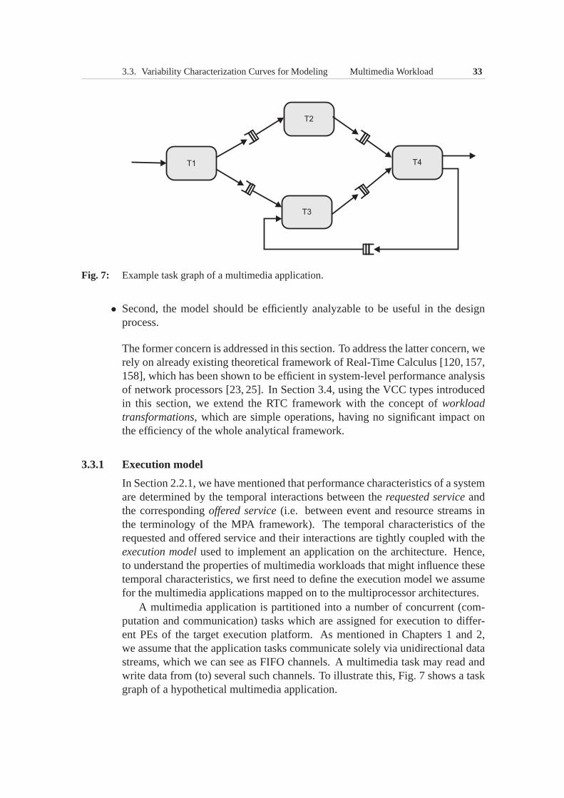
3.3. Variability Characterization Curves for Modeling Multimedia Workload 33
Fig. 7: Example task graph of a multimedia application.
• Second, the model should be efficiently analyzable to be useful in the designprocess.
The former concern is addressed in this section. To address the latter concern, werely on already existing theoretical framework of Real-TimeCalculus [120, 157,158], which has been shown to be efficient in system-level performance analysisof network processors [23, 25]. In Section 3.4, using the VCC types introducedin this section, we extend the RTC framework with the conceptof workloadtransformations, which are simple operations, having no significant impact onthe efficiency of the whole analytical framework.
3.3.1 Execution model
In Section 2.2.1, we have mentioned that performance characteristics of a systemare determined by the temporal interactions between therequested serviceandthe correspondingoffered service(i.e. between event and resource streams inthe terminology of the MPA framework). The temporal characteristics of therequested and offered service and their interactions are tightly coupled with theexecution modelused to implement an application on the architecture. Hence,to understand the properties of multimedia workloads that might influence thesetemporal characteristics, we first need to define the execution model we assumefor the multimedia applications mapped on to the multiprocessor architectures.
A multimedia application is partitioned into a number of concurrent (com-putation and communication) tasks which are assigned for execution to differ-ent PEs of the target execution platform. As mentioned in Chapters 1 and 2,we assume that the application tasks communicate solely viaunidirectional datastreams, which we can see as FIFO channels. A multimedia taskmay read andwrite data from (to) several such channels. To illustrate this, Fig. 7 shows a taskgraph of a hypothetical multimedia application.
34 Chapter 3. Modeling Variable Workload
We refer to the elementary data unit that a particular task can read from (writeto) a particular channel asstream object. A stream object might be a bit belong-ing to a compressed bitstream representing a coded video clip, or a macroblock,or a video frame, or an audio sample — depending on where in thetask graphthe corresponding stream exists.
A task becomes active whenever there is a predetermined amount of streamobjects available in the incoming channels. There may be some activation rulesassociated with the task [181]. These rules define specific conditions on the in-coming channels upon which this task is activated (e.g. availability of a specifiednumber of stream objects inall or only insomeincoming channels).
Whenever the task is activated it requests from the PE on whichit executes acertain amount of processor cycles. The task also consumes from the incomingchannels a number of stream objects. We assume that this number equals tothe amount of stream objects that were necessary to trigger the task. Whileexecuting (i.e. consuming the processor cycles) the task may write data intooutgoing channels. We assume non-blocking writing.
Finally, a sequence of task activations can be abstractly seen as arequeststream; and the availability of the PE for processing this stream can be seen as aresource stream.
3.3.2 Definitions of multimedia VCC types
The key workload characteristics to be captured in the workload model are thosecharacteristics that affect the timing properties of the request and resource streamsand their interactions. In this subsection, we pinpoint these key characteristicsand define VCC types to characterize them. Some of the VCC types that willbe introduced below are indicated in Fig. 8, which shows an abstract view of amultimedia task.
Event-based arrival curvesThe timing of task’s requests for service is influenced by thetiming of arrivals ofstream objects into the incoming channels of this task. These arrivals depend onthe tasks writing into these incoming channels (or on the system’s environment,if the stream is received from outside of the system). Each arrival into a channelcan be modeled as an event. Hence, a sequence of arrivals intoa given channelcan be represented as an event stream. Similar to the characterization modeldescribed in Section 2.2.2, we model the timing properties of such event streamswith VCCs calledevent-based arrival curves[85, 158].
Def. 5: (Event-Based Arrival Curves α = (αl, αu)) A lower event-based arrival curveαl and an upper event-based arrival curveαu are VCCs characterizing timingproperties of a given event stream.αl(∆) bounds from below andαu(∆) fromabove the number of events that can occur in the stream within any time intervalof length∆.
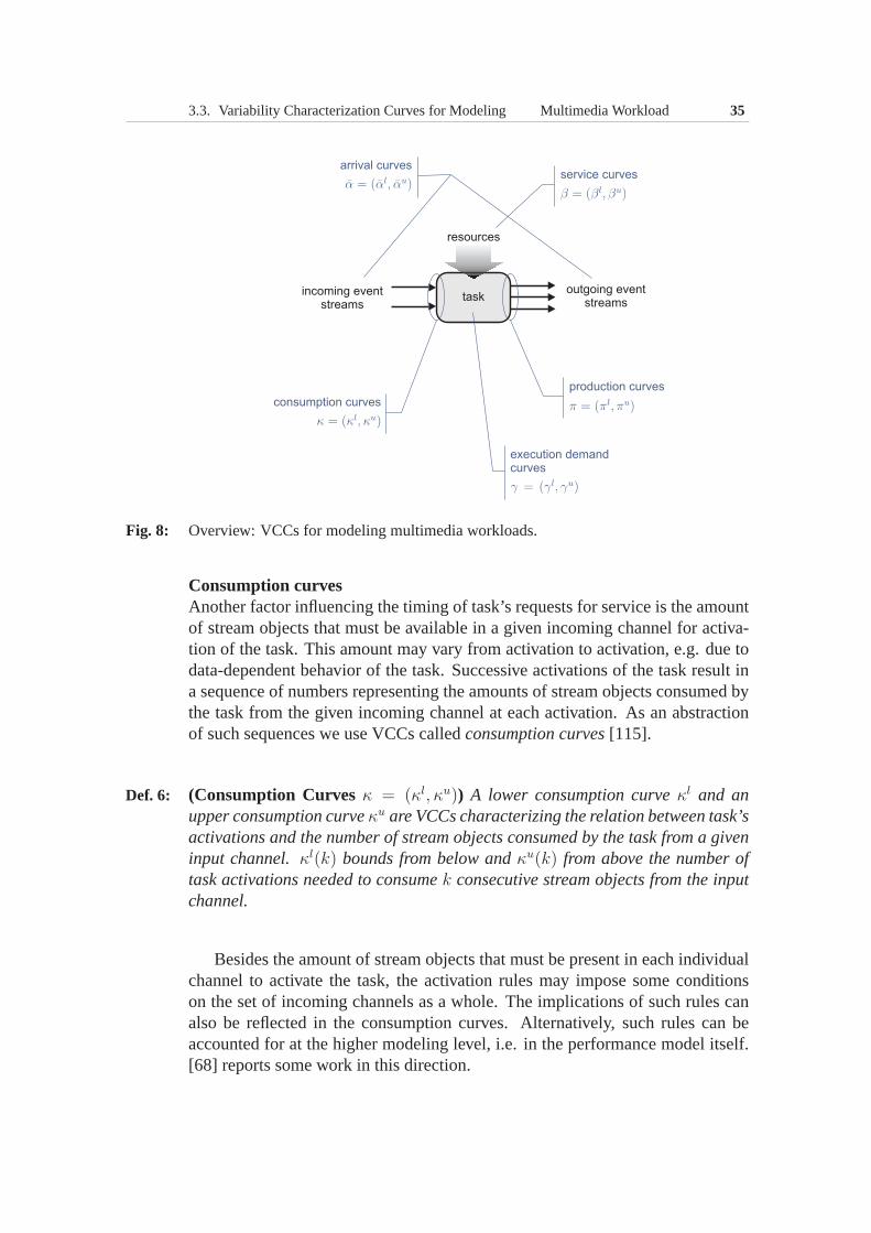
3.3. Variability Characterization Curves for Modeling Multimedia Workload 35
Fig. 8: Overview: VCCs for modeling multimedia workloads.
Consumption curvesAnother factor influencing the timing of task’s requests forservice is the amountof stream objects that must be available in a given incoming channel for activa-tion of the task. This amount may vary from activation to activation, e.g. due todata-dependent behavior of the task. Successive activations of the task result ina sequence of numbers representing the amounts of stream objects consumed bythe task from the given incoming channel at each activation.As an abstractionof such sequences we use VCCs calledconsumption curves[115].
Def. 6: (Consumption Curvesκ = (κl, κu)) A lower consumption curveκl and anupper consumption curveκu are VCCs characterizing the relation between task’sactivations and the number of stream objects consumed by thetask from a giveninput channel.κl(k) bounds from below andκu(k) from above the number oftask activations needed to consumek consecutive stream objects from the inputchannel.
Besides the amount of stream objects that must be present in each individualchannel to activate the task, the activation rules may impose some conditionson the set of incoming channels as a whole. The implications of such rules canalso be reflected in the consumption curves. Alternatively,such rules can beaccounted for at the higher modeling level, i.e. in the performance model itself.[68] reports some work in this direction.
36 Chapter 3. Modeling Variable Workload
Execution demand curvesThe amount of execution resources requested by a task at eachactivation mayvary depending, for example, on the task’s current state andthe values of processedstream objects, or on such architectural features as caches, branch predictors andpipelines. A sequence of task activations results in a sequence of execution de-mands imposed by the task on the PE. For modeling such sequences we useexecution demand curves[113, 115].
Def. 7: (Execution Demand Curvesγ = (γl, γu)) A lower execution demand curveγl and an upper execution demand curveγu are VCCs characterizing executiondemand of a given task.γu(k) bounds from above andγl(k) from below theamount of resource units (such as processor cycles) needed to complete anykconsecutive task executions.
Production curvesThe timing properties of event streams generated by a task atits outputs dependon the amount of stream objects produced by the task into the outgoing channelsat each activation. Again, from activation to activation this amount may vary. Tocharacterize this aspect of task’s activation sequences, we employ VCCs calledproduction curves[115].
Def. 8: (Production Curves π = (πl, πu)) A lower production curveπl and an upperproduction curveπu are VCCs characterizing the relation between task’s execu-tions and the number of stream objects produced by the task into a given outputchannel.πl(k) bounds from below andπu(k) from above the number of streamobjects produced by the task into the output channel as a result of k consecutiveexecutions of this task.
Resource-based service curvesAn important factor largely influencing the performance characteristics is avail-ability of execution resources for a given task over the time. Several tasksmapped onto a single PE may compete for the execution resource of this PE.A scheduling or arbitration policy then determines in whichorder these tasks areto be executed on the PE. As a consequence, the supply of resources to the tasksis not anymore uniformly distributed in time. This variability of the PE’s process-ing capacity as seen by an individual task is characterized using resource-basedservice curves[113, 115].
Def. 9: (Resource-Based Service Curvesβ = (βl, βu)) A lower resource-based servicecurveβl and an upper resource-based service curveβu are VCCs characterizingthe service offered to a given task on a given execution resource. βl(∆) boundsfrom below the number of resource units (such as processor cycles) that areguaranteedto be provided to the task within any time interval of length∆. βu(∆)
3.4. Workload Transformations 37
bounds from above the number of resource units thatcanbe provided to the taskwithin any time interval of length∆.
Type rate curvesIn some cases, for the performance analysis it is useful to distinguish within anevent stream (or any other sequence) different event types.For instance, thismight be useful in case if different event types impose different execution de-mands on a PE. The different event types may follow in variouspatterns withinthe stream. For the characterization of these patterns we employ so calledtyperate curves[166].
Def. 10: (Type Rate Curvesϑ = (ϑl, ϑu)) A lower type rate curveϑl and an upper typerate curveϑu are VCCs characterizing the containment of a given event type in agiven event stream.ϑl(k) bounds from below andϑu(k) from above the numberof events of the given type in any subsequence ofk consecutive events within theevent stream.
Event-based service curves and resource-based arrival curvesIn contrast to the resource-based service curves, the event-based service curvesexpress the availability of a PE for a given task in terms of the task executionsin-stead of processor cycles. Similarly, in contrast to the event-based arrival curves,the resource-based arrival curves express the amount ofresources(e.g. processorcycles) requested by a task.
Def. 11: (Event-Based Service Curvesβ = (βl, βu)) A lower event-based service curveβl and an upper event-based service curveβu are VCCs characterizing the ser-vice offered to a given task on a given execution resource.βl(∆) bounds frombelow the number of task executions that areguaranteedto be completed withinany time interval of length∆. βu(∆) bounds from above the number of taskexecutions thatcanbe completed within any time interval of length∆.
Def. 12: (Resource-Based Arrival Curvesα = (αl, αu)) A lower resource-based arrivalcurveαl(∆) and an upper resource-based arrival curveαu(∆) are VCCs char-acterizing the service requested by a given task from a givenexecution resource.αl(∆) bounds from below andαu(∆) from above the number ofresource units(such as processor cycles) that may be requested by the task within any timeinterval of length∆.
3.4 Workload TransformationsBeing able to analytically compute different performance figures of a system re-quires both the requested and the offered service being expressed in common
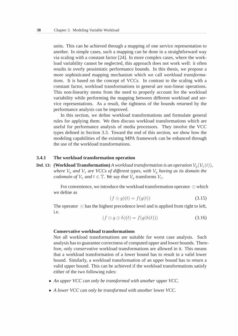
38 Chapter 3. Modeling Variable Workload
units. This can be achieved through a mapping of one service representation toanother. In simple cases, such a mapping can be done in a straightforward wayvia scaling with a constant factor [24]. In more complex cases, where the work-load variability cannot be neglected, this approach does not work well: it oftenresults in overly pessimistic performance bounds. In this thesis, we propose amore sophisticated mapping mechanism which we callworkload transforma-tions. It is based on the concept of VCCs. In contrast to the scaling with aconstant factor, workload transformations in general are non-linear operations.This non-linearity stems from the need to properly account for the workloadvariability while performing the mapping between different workload and ser-vice representations. As a result, the tightness of the bounds returned by theperformance analysis can be improved.
In this section, we define workload transformations and formulate generalrules for applying them. We then discuss workload transformations which areuseful for performance analysis of media processors. They involve the VCCtypes defined in Section 3.3. Toward the end of this section, we show how themodeling capabilities of the existing MPA framework can be enhanced throughthe use of the workload transformations.
3.4.1 The workload transformation operation
Def. 13: (Workload Transformation) A workload transformation is an operationVy(Vx(t)),whereVy andVx are VCCs of different types, withVy having as its domain thecodomain ofVx andt ∈ T. We say thatVy transformsVx.
For convenience, we introduce the workload transformationoperator⊙whichwe define as
(f ⊙ g)(t) = f(g(t)) (3.15)
The operator⊙ has the highest precedence level and is applied from right toleft,i.e.
(f ⊙ g ⊙ h)(t) = f(g(h(t))) (3.16)
Conservative workload transformationsNot all workload transformations are suitable for worst case analysis. Suchanalysis has to guarantee correctness of computed upper andlower bounds. There-fore, onlyconservativeworkload transformations are allowed in it. This meansthat a workload transformation of a lower bound has to resultin a valid lowerbound. Similarly, a workload transformation of an upper bound has to return avalid upper bound. This can be achieved if the workload transformations satisfyeither of the two following rules:
• An upper VCC can only be transformed with anotherupperVCC.
• A lower VCC can only be transformed with anotherlowerVCC.
3.4. Workload Transformations 39
f ⊙ g g =
Vu V l Vu−1 V l−1
Vu√ √
f = V l√ √
Vu−1 √ √
V l−1 √ √
Tab. 1: Conservative workload transformations (marked with√
).
Tab. 1 lists all possible workload transformations which satisfy the above rules.2
3.4.2 Workload transformations for multimedia VCCs
This subsection describes a set of conservative workload transformations whichare defined on the multimedia VCC types proposed in Section 3.3. These trans-formations are needed to extend the existing RTC-based performance analysisframework introduced in Chapter 2. They significantly improve the modeling ca-pabilities of the framework and thereby enable an accurate performance analysisof distributed execution platforms under multimedia workloads characterized bythe variability of several parameters. This subsection explains the role of each in-dividual transformation within the RTC-based performance analysis framework.
Suppose that different properties of the system whose performance we wishto analyze are specified using a subset of VCCs which were definedin Sec-tion 3.3. For the performance analysis, we need to build a performance modelout of these VCCs. The first step in constructing such a model is to quantify therequested and the offered service in some common units. The choice of unitsdepends on particular goals of the analysis and on the input specification. Aswe will see later in this chapter (in Section 3.4.3), within asingle performancemodel we may need to carry out some computations using resource-based unitsand other computations using event-based units. Hence, a variety of workloadtransformations may be required during constructing a performance model. Inwhat follows, we list and explain different sorts of workload transformationswhich can be useful in the performance analysis.
Input stream arrivals −→ task activationsThis workload transformation maps the arrival process of a stream to the activa-tion process of the task which processes this stream. The timing of the activationprocess depends on the timing of the stream arrivals. This isbecause, according
2To correctly interpret Tab. 1, recall Props. 3 and 4 shown in Section 3.2, stating that thepseudo-inverse of an upper VCC is a lower VCC, and the pseudo-inverse of a lower VCC is anupper VCC.
40 Chapter 3. Modeling Variable Workload
to our model of computation, a task is activated only if the number of streamobjects present at its input is larger or equal to the amount of stream objects thatthe task will consume during its next execution. The stream’s arrival process isspecified by event-based arrival curves(αl
I , αuI ). The goal of the workload trans-
formation is to obtain arrival curves(αlta, α
uta)(∆) that represent upper and lower
bounds on the number of tasks activations which may occur in any time interval∆. The workload transformation can be performed using consumption curves(κl, κu) as follows.
αuta(∆) = (κu ⊙ αu
I )(∆) (3.17)
αlta(∆) = (κl ⊙ αl
I)(∆) (3.18)
Task activations−→ execution demandThis workload transformation maps the activation process of a task to the exe-cution demand imposed by this task on the resource on which itexecutes. Theamount of the imposed execution demand, measured in resource-based units pertime interval, depends on the timing of the task activationsand on the execu-tion demand imposed by each individual activation. The goalof this workloadtransformation is to obtain arrival curves(αl
I , αuI )(∆) which represent upper and
lower bounds on the number of resource units that can be requested by the taskwithin any time interval∆. Suppose that the timing of task activations is givenby arrival curves(αl
ta, αuta) as defined by (3.17) and (3.18). Then using execution
demand curves(γl, γu) we can transform(αlta, α
uta) into (αl
I , αuI ) as follows.
αuI (∆) = (γu ⊙ αu
ta)(∆) (3.19)
αlI(∆) = (γl ⊙ αl
ta)(∆) (3.20)
Input stream arrivals −→ execution demandCombining (3.17) with (3.19) and (3.18) with (3.20) gives a mapping of streamarrivals expressed in number of stream objects (i.e. in event-based quantities) pertime interval on to the execution demand which is imposed by this stream on theexecution resource. The execution demand is then expressedin resource-basedquantities per time interval.
αuI (∆) = (γu ⊙ κu ⊙ αu
I )(∆) (3.21)
αlI(∆) = (γl ⊙ κl ⊙ αl
I)(∆) (3.22)
The resulting resource-based arrival curves(αlI , α
uI ) can be combined in RTC
computations with resource-based service curves(βl, βu). Note that if a taskalways consumes only one stream object per one execution, i.e. if κu(k) =κl(k) = k, then (3.21) and (3.22) can be reduced to
αuI (∆) = (γu ⊙ αu
I )(∆) (3.23)
αlI(∆) = (γl ⊙ αl
I)(∆) (3.24)
3.4. Workload Transformations 41
Consumed resources−→ task executionsSuppose we know resource-based arrival curves(αl
O, αuO)(∆) which represent
the upper and lower bounds on the amount of resource units that a task may con-sume within any time interval∆. The goal of this workload transformation is toconvert these arrival curves into arrival curves(αl
te, αute) that represent the upper
and lower bounds on the number of task executions that could be performed forthe given amount of resources modeled by(αl
O, αuO)(∆). This workload trans-
formation can be performed through pseudo-inverses of the execution demandcurves as follows.
αute(∆) = (γl−1 ⊙ αu
O)(∆) (3.25)
αlte(∆) = (γu−1 ⊙ αl
O)(∆) (3.26)
Task executions−→ output stream arrivalsThis workload transformation maps the execution process ofa task to the arrivalprocess of a stream produced by this task. The timing of the stream arrivalsdepends on the timing of task executions (since the task can produce streamobjects only as a result of its execution). In addition, the amount of producedstream objects may vary from execution to execution. The goal of this workloadtransformation is to obtain event-based arrival curves of the stream at the outputof the task, i.e.(αl
O, αuO). Let (αl
te, αute)(∆) denote arrival curves that represent
upper and lower bounds on the number of the task executions that can occur inany time interval∆. Then, using production curves(πl, πu), we can perform therequired workload transformation as follows.
αuO(∆) = (πu ⊙ αu
te)(∆) (3.27)
αlO(∆) = (πl ⊙ αl
te)(∆) (3.28)
Consumed resources−→ output stream arrivalsCombining (3.25) with (3.27) and (3.26) with (3.28) gives a mapping of theamount of resources consumed by a task per time interval to the number ofstream objects produced by this task per time interval. Thisworkload trans-formation is performed as follows.
αuO(∆) = (πu ⊙ γl−1 ⊙ αu
O)(∆) (3.29)
αlO(∆) = (πl ⊙ γu−1 ⊙ αl
O)(∆) (3.30)
Note that if a task always produces only one stream object perone execution, i.e.if πu(k) = πl(k) = k, then (3.29) and (3.30) can be reduced to
αuO(∆) = (γl−1 ⊙ αu
O)(∆) (3.31)
αlO(∆) = (γu−1 ⊙ αl
O)(∆) (3.32)

42 Chapter 3. Modeling Variable Workload
Offered resources−→ task executionsThe goal of this workload transformation is to map the amountof resourceswhich a task is offered per time interval to the number of executions that thistask can perform per time interval if it uses the offered amount of resources.The offered amount of resources is modeled by resource-based service curves(βl, βu). The number of executions which can be performed for the offerednumber of resources per time interval is modeled by event-based service curves(βl, βu). The workload transformation can be achieved using pseudo-inverses ofthe execution demand curves as follows.
βu(∆) = (γl−1 ⊙ βu)(∆) (3.33)
βl(∆) = (γu−1 ⊙ βl)(∆) (3.34)
Task executions−→ offered resourcesThe goal of this workload transformation is to map the service expressed in num-ber of task executions (i.e. in event-based quantities) which can be performed pertime interval on to the amount of resources which are necessary per time intervalin order to offer this service. The number of task executionsofferedper timeinterval is modeled by event-based service curves(βl, βu), and the amount ofresource units offered per time interval is modeled by resource-based servicecurves(βl, βu). The workload transformation is performed via execution de-mand curves(γl, γu) as follows.
βu(∆) = (γu ⊙ βu)(∆) (3.35)
βl(∆) = (γl ⊙ βl)(∆) (3.36)
3.4.3 Extended Modular Performance Analysis Framework
This subsection explains how the MPA framework described inSection 2.2 canbe extended with the workload transformations introduced in the previous sub-section.
The workload transformations can be applied at different points within ascheduling network. Since the transformations must be conservative, each trans-formation is typically associated with some loss of accuracy of the bounds.Hence, as a rule of thumb, the total number of workload transformations withina scheduling network should be minimized. There is, however, a more specificguideline for the optimal placement of the workload transformations within ascheduling network. We elaborate on it now.
If we use Real-Time Calculus to analyze a scheduling network then all eventand resource flows in the network are modeled with arrival andservice curves. Ingeneral, we are free to choose whether an arrival (service) curve existing betweenany two performance components is expressed in event-basedor resource-based
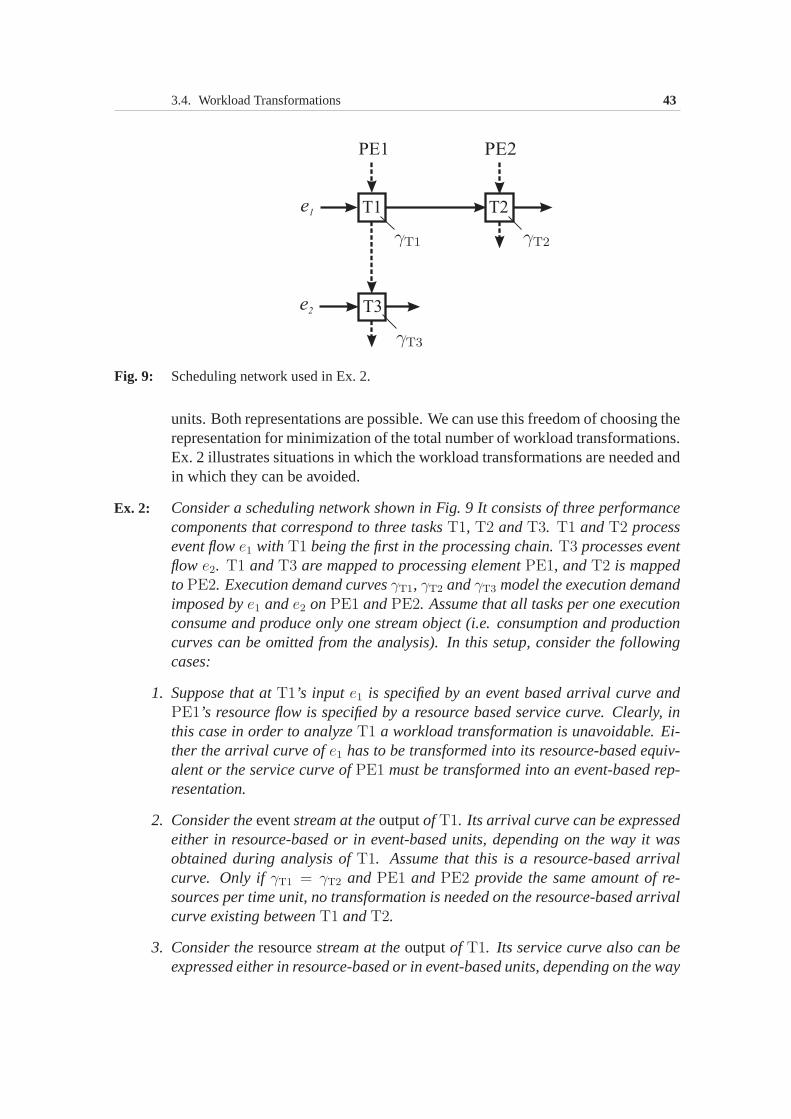
3.4. Workload Transformations 43
T1 T2
T3
e1
e2
PE1 PE2
Fig. 9: Scheduling network used in Ex. 2.
units. Both representations are possible. We can use this freedom of choosing therepresentation for minimization of the total number of workload transformations.Ex. 2 illustrates situations in which the workload transformations are needed andin which they can be avoided.
Ex. 2: Consider a scheduling network shown in Fig. 9 It consists of three performancecomponents that correspond to three tasksT1, T2 andT3. T1 andT2 processevent flowe1 with T1 being the first in the processing chain.T3 processes eventflow e2. T1 andT3 are mapped to processing elementPE1, andT2 is mappedto PE2. Execution demand curvesγT1, γT2 andγT3 model the execution demandimposed bye1 ande2 onPE1 andPE2. Assume that all tasks per one executionconsume and produce only one stream object (i.e. consumption and productioncurves can be omitted from the analysis). In this setup, consider the followingcases:
1. Suppose that atT1’s input e1 is specified by an event based arrival curve andPE1’s resource flow is specified by a resource based service curve. Clearly, inthis case in order to analyzeT1 a workload transformation is unavoidable. Ei-ther the arrival curve ofe1 has to be transformed into its resource-based equiv-alent or the service curve ofPE1 must be transformed into an event-based rep-resentation.
2. Consider theeventstream at theoutputof T1. Its arrival curve can be expressedeither in resource-based or in event-based units, depending on the way it wasobtained during analysis ofT1. Assume that this is a resource-based arrivalcurve. Only ifγT1 = γT2 and PE1 and PE2 provide the same amount of re-sources per time unit, no transformation is needed on the resource-based arrivalcurve existing betweenT1 andT2.
3. Consider theresourcestream at theoutputof T1. Its service curve also can beexpressed either in resource-based or in event-based units, depending on the way
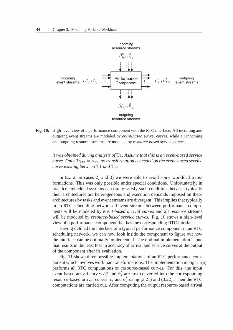
44 Chapter 3. Modeling Variable Workload
PerformanceComponent
incomingevent streams
outgoingevent streams
outgoingresource streams
incomingresource streams
Fig. 10: High-level view of a performance component with the RTC interface. All incoming andoutgoing event streams are modeled byevent-basedarrival curves, while all incomingand outgoing resource streams are modeled byresource-basedservice curves.
it was obtained during analysis ofT1. Assume that this is an event-based servicecurve. Only ifγT1 = γT3, no transformation is needed on the event-based servicecurve existing betweenT1 andT3.
In Ex. 2, in cases 2) and 3) we were able to avoid some workload trans-formations. This was only possible under special conditions. Unfortunately, inpractice embedded systems can rarely satisfy such conditions because typicallytheir architectures are heterogeneous and execution demands imposed on thesearchitectures by tasks and event streams are divergent. This implies that typicallyin an RTC scheduling network all event streams between performance compo-nents will be modeled byevent-based arrival curvesand all resource streamswill be modeled byresource-based service curves. Fig. 10 shows a high-levelview of a performance component that has the corresponding RTC interface.
Having defined the interface of a typical performance component in an RTCscheduling network, we can now look inside the component to figure out howthe interface can be optimally implemented. The optimal implementation is onethat results in the least loss in accuracy of arrival and service curves at the outputof the component after its evaluation.
Fig. 11 shows three possible implementations of an RTC performance com-ponent which involves workload transformations. The implementation in Fig. 11(a)performs all RTC computations on resource-based curves. For this, the inputevent-based arrival curvesαu
I andαlI are first converted into the corresponding
resource-based arrival curvesαuI andαl
I using (3.21) and (3.22). Then the RTCcomputations are carried out. After computing the output resource-based arrival
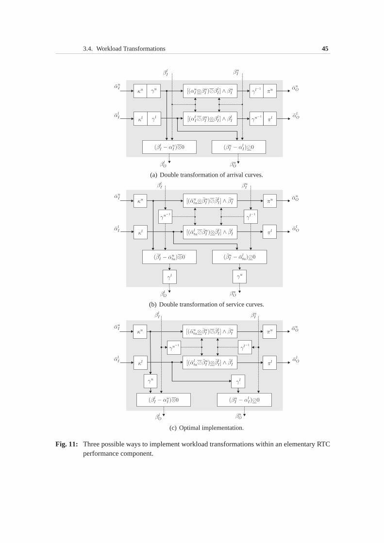
3.4. Workload Transformations 45
(a) Double transformation of arrival curves.
(b) Double transformation of service curves.
(c) Optimal implementation.
Fig. 11: Three possible ways to implement workload transformations within an elementaryRTCperformance component.
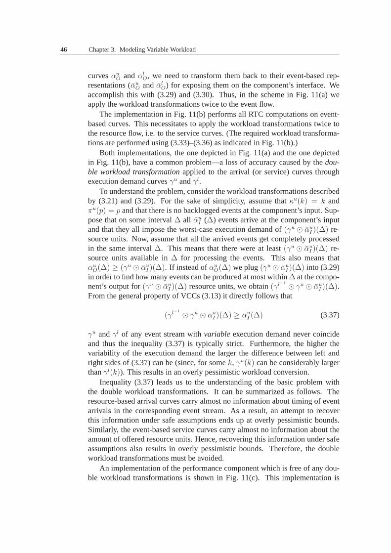
46 Chapter 3. Modeling Variable Workload
curvesαuO andαl
O, we need to transform them back to their event-based rep-resentations (αu
O andαlO) for exposing them on the component’s interface. We
accomplish this with (3.29) and (3.30). Thus, in the scheme in Fig. 11(a) weapply the workload transformations twice to the event flow.
The implementation in Fig. 11(b) performs all RTC computations on event-based curves. This necessitates to apply the workload transformations twice tothe resource flow, i.e. to the service curves. (The required workload transforma-tions are performed using (3.33)–(3.36) as indicated in Fig. 11(b).)
Both implementations, the one depicted in Fig. 11(a) and the one depictedin Fig. 11(b), have a common problem—a loss of accuracy caused by thedou-ble workload transformationapplied to the arrival (or service) curves throughexecution demand curvesγu andγl.
To understand the problem, consider the workload transformations describedby (3.21) and (3.29). For the sake of simplicity, assume thatκu(k) = k andπu(p) = p and that there is no backlogged events at the component’s input. Sup-pose that on some interval∆ all αu
I (∆) events arrive at the component’s inputand that they all impose the worst-case execution demand of(γu ⊙ αu
I )(∆) re-source units. Now, assume that all the arrived events get completely processedin the same interval∆. This means that there were at least(γu ⊙ αu
I )(∆) re-source units available in∆ for processing the events. This also means thatαu
O(∆) ≥ (γu ⊙ αuI )(∆). If instead ofαu
O(∆) we plug(γu ⊙ αuI )(∆) into (3.29)
in order to find how many events can be produced at most within∆ at the compo-nent’s output for(γu ⊙ αu
I )(∆) resource units, we obtain(γl−1 ⊙ γu ⊙ αuI )(∆).
From the general property of VCCs (3.13) it directly follows that
(γl−1 ⊙ γu ⊙ αuI )(∆) ≥ αu
I (∆) (3.37)
γu andγl of any event stream withvariable execution demand never coincideand thus the inequality (3.37) is typically strict. Furthermore, the higher thevariability of the execution demand the larger the difference between left andright sides of (3.37) can be (since, for somek, γu(k) can be considerably largerthanγl(k)). This results in an overly pessimistic workload conversion.
Inequality (3.37) leads us to the understanding of the basicproblem withthe double workload transformations. It can be summarized as follows. Theresource-based arrival curves carry almost no informationabout timing of eventarrivals in the corresponding event stream. As a result, an attempt to recoverthis information under safe assumptions ends up at overly pessimistic bounds.Similarly, the event-based service curves carry almost no information about theamount of offered resource units. Hence, recovering this information under safeassumptions also results in overly pessimistic bounds. Therefore, the doubleworkload transformations must be avoided.
An implementation of the performance component which is free of any dou-ble workload transformations is shown in Fig. 11(c). This implementation is
3.5. Obtaining Variability Characterization Curves 47
optimal in a sense that it minimizes the inaccuracy introduced into the resultingbounds as a result of workload transformations.
SummaryIn this subsection, we addressed the problem of extending the existing MPAframework with workload transformations. We showed that inorder to avoida considerable loss of accuracy while introducing the workload transformationsinto an RTC scheduling network, the following two principles have to be fol-lowed:
• the total number of workload transformations in a network should be minimized;
• the double workload transformations should be avoided.
Based on these principles we developed a mathematical model of an RTC per-formance component which can be used in the extended MPA framework. Themodel represents the main result of this subsection. It is captured by the follow-ing set of equations:
αuO = πu ⊙ ([(κu ⊙ αu
I ⊗ γl−1 ⊙ βuI )⊘ γu−1 ⊙ βl
I ] ∧ γl−1 ⊙ βuI ) (3.38)
αlO = πl ⊙ ([(κl ⊙ αl
I ⊘ γl−1 ⊙ βuI )⊗ γu−1 ⊙ βl
I ] ∧ γu−1 ⊙ βlI) (3.39)
βuO = (βu
I − γl ⊙ κl ⊙ αlI)⊘ 0 (3.40)
βlO = (βl
I − γu ⊙ κu ⊙ αuI )⊗ 0 (3.41)
3.5 Obtaining Variability Characterization CurvesThe quality of results delivered by performance evaluationand scheduling meth-ods using VCCs largely depends on the quality of VCCs supplied to them as aninput for the analysis. The quality of the VCCs, in turn, depends on the wayin which they have been obtained. This section discusses relevant issues andoutlines several approaches to obtaining VCCs.
3.5.1 Objectives and limitations
Recall from Section 3.2 that a VCC is essentially an upper or a lower boundonthe worst-case or, respectively, best-case variability offunctions belonging to agiven set. Hence, any considerations that can be made about worst-case boundsin general are also applicable to VCCs. Nevertheless, to provide a framework fora discussion of different ways for obtaining VCCs, in this subsection we revisitsome of the relevant general issues by putting them in the VCC context.
At least two objectives have to be pursued while obtaining a VCC:
48 Chapter 3. Modeling Variable Workload
• Guarantee: A VCC has to guarantee that itfully captures the worst-case (orbest-case) variability of a given function set, i.e. it has to be a proper bound.This guarantee is a necessary condition for obtaining reliable results from anyanalysis based on the given VCC.
• Tightness: A VCC has to be as tight as possible. The tightness of the VCC caninfluence the accuracy of the analytical results. The tighter the VCC the moreaccurate variability characterization it provides and, hence, the more accurateanalytical results can be achieved through its use.
In order to see the whole range of possibilities for obtaining VCCs we haveto make a clear distinction between a given set of increasingfunctions to be char-acterized by a VCC (refer to Defs. 1 and 2) and the information based on whichthe VCC characterizing this set is constructed. We refer to such information asthe source information. In the simplest case the source information representsthe function set itself. The corresponding VCC can then be derived directly fromthis set. In other cases the function set might not be explicitly available or itmay be incomplete, however, some knowledge about it still can be at our dis-posal. This knowledge, which can serve as the source information in such cases,may be in the form of assumptions, formal specifications, various bounds andparameter estimates pertaining to the system at hand or to its environment or toboth. Sections 3.5.2, 3.5.3 and 3.5.4 provide some concreteexamples of possibleforms of the source information.
Having drawn the distinction between the function set to be characterizedand the source information based on which a VCC is constructed, we make thefollowing assertions.
• The guarantee, which a VCC is required to provide, depends on the particularmodeling and analysis goals. These goals, therefore, determine the function setto be characterized by the VCC.
• Whether or not a VCC provides the required guarantee depends onhow guaran-teed (i.e. reliable and sufficient) is the source information based on which theVCC has been constructed and does not depend on a particular method used toconstruct it.3
• The tightness of a VCC depends on the accuracy of the source information aswell as on the method which has been used for constructing theVCC.
In summary, we identify the following principle limitations in achieving theobjectives set forth in the beginning of this subsection. The guarantee provided
3If the source information is reliable and sufficient for providing the required guarantee butnevertheless the resulting VCC does not provide this guarantee, then the method is wrong (e.g.contains some faults). We exclude such cases from the consideration by assuming that anymethod for obtaining VCCs is correct.
3.5. Obtaining Variability Characterization Curves 49
by a VCC is limited by the reliability and sufficiency of its source information,whereas the tightness of the VCC is limited by the accuracy of both the sourceinformation and the method by which the VCC has been obtained.
3.5.2 Obtaining VCCs from traces
As Section 3.5.1 mentions, one of the possible ways to obtaina VCC is to con-struct it directly from the function set which this VCC has to characterize (i.e. inthis case the source information for the VCC is the function set itself). Obviously,being able to obtain a guaranteed VCC in this way requires all the functions inthe set to be precisely defined. Furthermore, by constructing a VCC directlyfrom the function set we can obtain the tightest possible VCC for this set. Suchtightest upper and lower VCCscan be computed as defined below.
Def. 14: (Tightest Upper VCC) The tightest upper VCCVuA∗ for a given set of increasing
functionsA is computed as
VuA∗(s) = sup
∀Ai∈A, ∀t∈T
{Ai(t+ s) − Ai(t)} ∀s ∈ T (3.42)
Def. 15: (Tightest Lower VCC) The tightest lower VCCV lA∗
for a given set of increasingfunctionsA is computed as
V lA
∗(s) = inf
∀Ai∈A, ∀t∈T
{Ai(t+ s) − Ai(t)} ∀s ∈ T (3.43)
Showing thatVuA∗ computed with (3.42) is thetightestupper VCC forA is
straightforward: any other functionV , such thatV (s) < VuA∗(s) for somes, is
not an upper VCC forA by Def. 1. By following a similar reasoning,V lA∗
com-puted with (3.43) can be shown to be the tightest lower VCC.
In practice, the increasing functionsAi(t) from which a VCC is constructedcan be computed fromtraces. A trace is a sequence of events which have oc-curred as a result of a system execution at a given point in thesystem or itsenvironment (e.g. at a specified input or output or processing element). Letvj ∈ R≥0 andtj ∈ T denote, respectively, the value and the occurrence time ofjth event recorded in a trace. Then the increasing functionA corresponding tothis trace can be computed as follows.
A(t) =∑
j: tj≤t
vj and A(0) = 0
Traces are collected by measuring the parameters of interest in a real systemor its simulator. The event valuesvj can represent different parameters of thesystem’s behavior. For example, they can indicate arrivalsof events at an inputof the system, or they can be execution times of a task which are recorded into
50 Chapter 3. Modeling Variable Workload
the trace each time the task finishes its execution, etc. The occurrence timetjdoes not need to be an absolute time. It can also be a sequence number of anevent in the trace.
Note that in order to obtain the VCCs it is not necessary to first convertthe traces into the increasing functions. The VCCs can be constructed directlyfrom the traces. For this purpose, the traces are analyzed bysliding along themwindows of different sizes. The window size corresponds to the argument valuefor which a VCC is computed. The value of upper (lower) VCC for a givenargument value is then the maximum (the minimum) sum of tracevaluesvj thatfall into a window of the corresponding size.
DiscussionAlthough VCCs obtained from traces can accurately capture worst-case and best-case variability in the event streams, they have a restricted applicability. In partic-ular, such VCCs cannot be used for the timing analysis of hard real-time systems.The hard real-time analysis has to fully cover all possible system states and in-teractions with the environment. Hence, if such an analysisuses VCCs that havebeen obtained from a set of traces, then this set must containall possible traces.For most of the realistic systems, however, generating the exhaustive set of tracesis infeasible.
Despite their limitation mentioned above, the VCCs obtained from traceshave a wide range of applications in the analysis and design of soft real-timesystems. For this class of systems the full coverage of the analysis is not soessential as for the hard real-time systems. Some rare or exceptional systembehaviors can be omitted from the consideration especiallyin the context of asystem-level design space exploration. Therefore, a set oftraces representingtypical cases may be sufficient for obtaining a VCC for analysis of soft real-timesystems.
Since most of the multimedia systems belong to the class of soft real-timesystems, in this thesis for experimental case studies we useVCCs that have beenobtained from traces. Appendix A gives details on the simulation frameworkused to collect the traces and obtain from them the VCCs.
3.5.3 Obtaining VCCs from constraints
Sometimes no complete information is available about functionsAi belonging toa given setA to be characterized by VCCs. The set of functionsA might not beexplicitly defined or it might be defined only partially. For instance, exact valuesof functionsAi may not be known because of some uncertainty in parametersof a modeled system or its environment. In such situations the tightest upperand lower VCCs cannot be obtained using (3.42) and (3.43). ThenVCCs can beconstructed based on some other kind of source information than the function setitself. This subsection and Section 3.5.4 are devoted to a discussion of such ap-
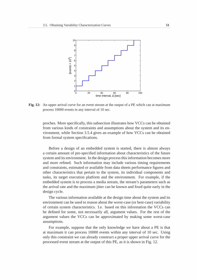
3.5. Obtaining Variability Characterization Curves 51
0 20 40 60 80 1000
1
2
3
4
5
6
7
8
9
10
time interval, ∆ [sec]
[eve
nts
× 10
4 ]
Fig. 12: An upper arrival curve for an event stream at the output of a PE which can at maximumprocess 10000 events in any interval of 10 sec.
proches. More specifically, this subsection illustrates how VCCs can be obtainedfrom various kinds of constraints and assumptions about thesystem and its en-vironment, while Section 3.5.4 gives an example of how VCCs canbe obtainedfrom formal system specifications.
Before a design of an embedded system is started, there is almost alwaysa certain amount of pre-specified information about characteristics of the futuresystem and its environment. In the design process this information becomes moreand more refined. Such information may include various timing requirementsand constraints, estimated or available from data sheets performance figures andother characteristics that pertain to the system, its individual components andtasks, its target execution platform and the environment. For example, if theembedded system is to process a media stream, the stream’s parameters such asthe arrival rate and the maximum jitter can be known and fixed quite early in thedesign cycle.
The various information available at the design time about the system and itsenvironment can be used to reason about the worst-case (or best-case) variabilityof certain system characteristics. I.e. based on this information the VCCs canbe defined for some, not necessarily all, argument values. For the rest of theargument values the VCCs can be approximated by making some worst-caseassumptions.
For example, suppose that the only knowledge we have about a PE is thatat maximum it can process 10000 events within any interval of10 sec. Usingonly this constraint we can already construct a proper upperarrival curve for theprocessed event stream at the output of this PE, as it is shownin Fig. 12.
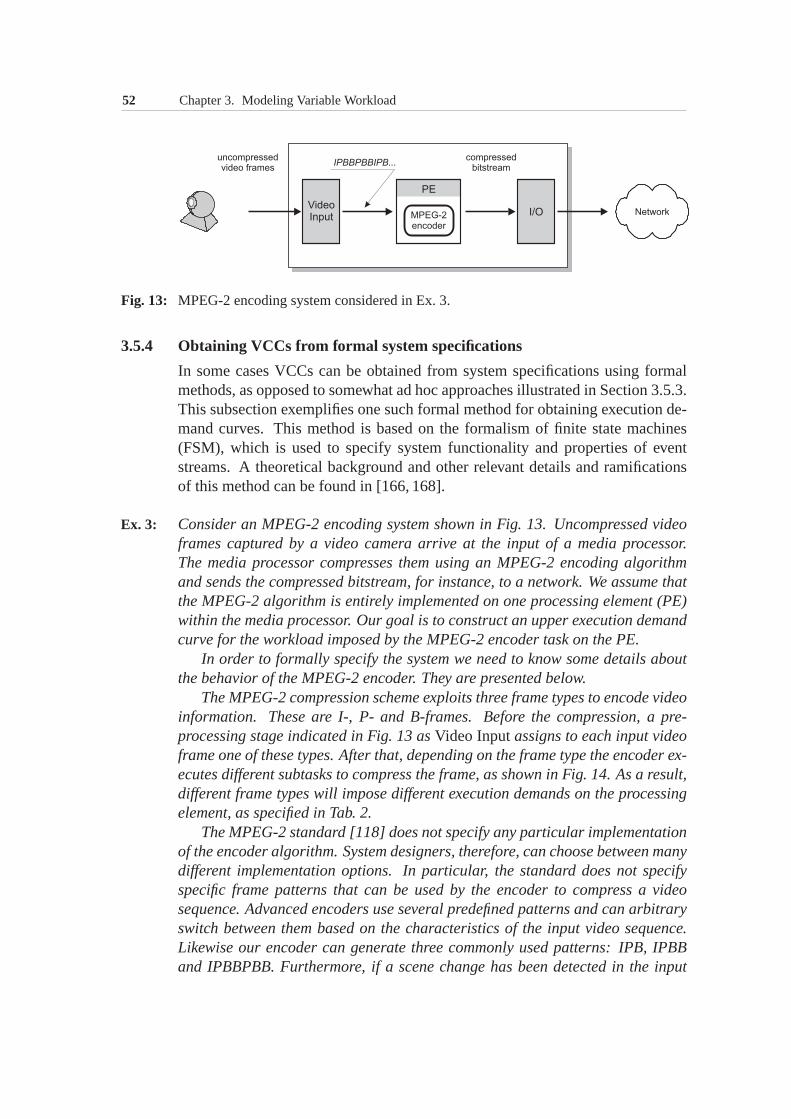
52 Chapter 3. Modeling Variable Workload
Fig. 13: MPEG-2 encoding system considered in Ex. 3.
3.5.4 Obtaining VCCs from formal system specifications
In some cases VCCs can be obtained from system specifications using formalmethods, as opposed to somewhat ad hoc approaches illustrated in Section 3.5.3.This subsection exemplifies one such formal method for obtaining execution de-mand curves. This method is based on the formalism of finite state machines(FSM), which is used to specify system functionality and properties of eventstreams. A theoretical background and other relevant details and ramificationsof this method can be found in [166, 168].
Ex. 3: Consider an MPEG-2 encoding system shown in Fig. 13. Uncompressed videoframes captured by a video camera arrive at the input of a media processor.The media processor compresses them using an MPEG-2 encoding algorithmand sends the compressed bitstream, for instance, to a network. We assume thatthe MPEG-2 algorithm is entirely implemented on one processing element (PE)within the media processor. Our goal is to construct an upper execution demandcurve for the workload imposed by the MPEG-2 encoder task on the PE.
In order to formally specify the system we need to know some details aboutthe behavior of the MPEG-2 encoder. They are presented below.
The MPEG-2 compression scheme exploits three frame types toencode videoinformation. These are I-, P- and B-frames. Before the compression, a pre-processing stage indicated in Fig. 13 asVideo Inputassigns to each input videoframe one of these types. After that, depending on the frame type the encoder ex-ecutes different subtasks to compress the frame, as shown in Fig. 14. As a result,different frame types will impose different execution demands on the processingelement, as specified in Tab. 2.
The MPEG-2 standard [118] does not specify any particular implementationof the encoder algorithm. System designers, therefore, canchoose between manydifferent implementation options. In particular, the standard does not specifyspecific frame patterns that can be used by the encoder to compress a videosequence. Advanced encoders use several predefined patterns and can arbitraryswitch between them based on the characteristics of the input video sequence.Likewise our encoder can generate three commonly used patterns: IPB, IPBBand IPBBPBB. Furthermore, if a scene change has been detected in the input
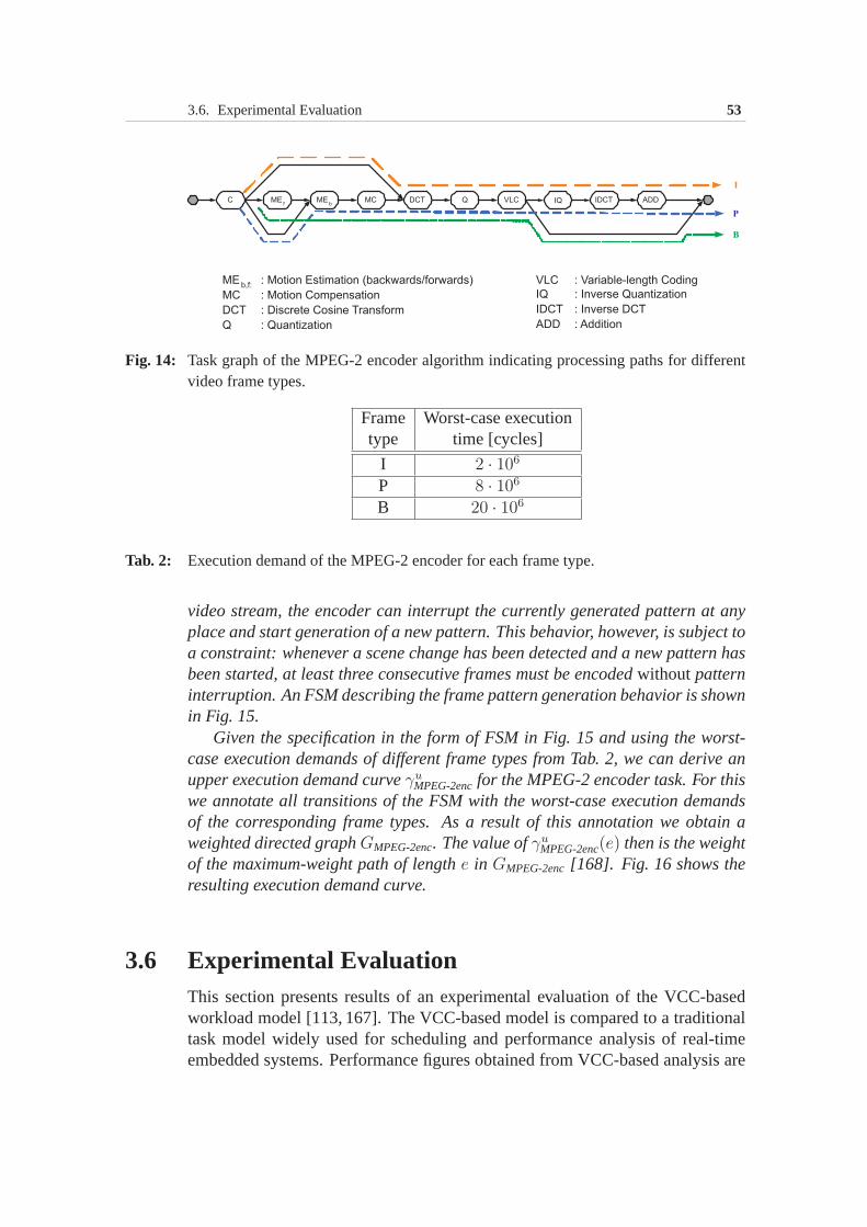
3.6. Experimental Evaluation 53
C MEf
MEb
QMC DCT VLC IQ IDCT ADD
I
P
B
MEb,f:
MC
DCT
Q
: Motion Estimation (backwards/forwards)
: Motion Compensation
: Discrete Cosine Transform
: Quantization
VLC
IQ
IDCT
ADD
: Variable-length Coding
: Inverse Quantization
: Inverse DCT
: Addition
Fig. 14: Task graph of the MPEG-2 encoder algorithm indicating processing pathsfor differentvideo frame types.
Frame Worst-case executiontype time [cycles]
I 2 · 106
P 8 · 106
B 20 · 106
Tab. 2: Execution demand of the MPEG-2 encoder for each frame type.
video stream, the encoder can interrupt the currently generated pattern at anyplace and start generation of a new pattern. This behavior, however, is subject toa constraint: whenever a scene change has been detected and a new pattern hasbeen started, at least three consecutive frames must be encodedwithout patterninterruption. An FSM describing the frame pattern generation behavior is shownin Fig. 15.
Given the specification in the form of FSM in Fig. 15 and using the worst-case execution demands of different frame types from Tab. 2,we can derive anupper execution demand curveγu
MPEG-2encfor the MPEG-2 encoder task. For thiswe annotate all transitions of the FSM with the worst-case execution demandsof the corresponding frame types. As a result of this annotation we obtain aweighted directed graphGMPEG-2enc. The value ofγu
MPEG-2enc(e) then is the weightof the maximum-weight path of lengthe in GMPEG-2enc[168]. Fig. 16 shows theresulting execution demand curve.
3.6 Experimental EvaluationThis section presents results of an experimental evaluation of the VCC-basedworkload model [113, 167]. The VCC-based model is compared to atraditionaltask model widely used for scheduling and performance analysis of real-timeembedded systems. Performance figures obtained from VCC-based analysis are
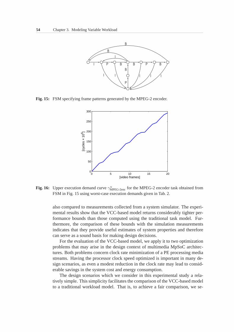
54 Chapter 3. Modeling Variable Workload
Fig. 15: FSM specifying frame patterns generated by the MPEG-2 encoder.
0 5 10 15 200
50
100
150
200
250
300
[video frames]
[cyc
les
× 10
6 ]
Fig. 16: Upper execution demand curveγuMPEG-2encfor the MPEG-2 encoder task obtained from
FSM in Fig. 15 using worst-case execution demands given in Tab. 2.
also compared to measurements collected from a system simulator. The experi-mental results show that the VCC-based model returns considerably tighter per-formance bounds than those computed using the traditional task model. Fur-thermore, the comparison of these bounds with the simulation measurementsindicates that they provide useful estimates of system properties and thereforecan serve as a sound basis for making design decisions.
For the evaluation of the VCC-based model, we apply it to two optimizationproblems that may arise in the design context of multimedia MpSoC architec-tures. Both problems concern clock rate minimization of a PE processing mediastreams. Having the processor clock speed optimized is important in many de-sign scenarios, as even a modest reduction in the clock rate may lead to consid-erable savings in the system cost and energy consumption.
The design scenarios which we consider in this experimentalstudy a rela-tively simple. This simplicity facilitates the comparisonof the VCC-based modelto a traditional workload model. That is, to achieve a fair comparison, we se-
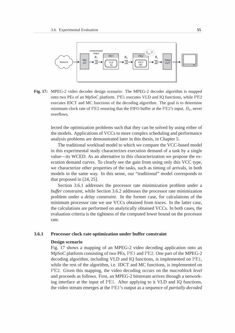
3.6. Experimental Evaluation 55
Fig. 17: MPEG-2 video decoder design scenario: The MPEG-2 decoder algorithm is mappedonto two PEs of an MpSoC platform.PE1 executes VLD and IQ functions, whilePE2
executes IDCT and MC functions of the decoding algorithm. The goal is to determineminimum clock rate ofPE2 ensuring that the FIFO buffer at thePE2’s input,B2, neveroverflows.
lected the optimization problems such that they can be solved by using either ofthe models. Applications of VCCs to more complex scheduling and performanceanalysis problems are demonstrated later in this thesis, inChapter 5.
The traditional workload model to which we compare the VCC-based modelin this experimental study characterizes execution demandof a task by a singlevalue—its WCED. As an alternative to this characterization wepropose the ex-ecution demand curves. To clearly see the gain from using only this VCC type,we characterize other properties of the tasks, such as timing of arrivals, in bothmodels in the same way. In this sense, our “traditional” model corresponds tothat proposed in [24, 25].
Section 3.6.1 addresses the processor rate minimization problem under abuffer constraint, while Section 3.6.2 addresses the processor rate minimizationproblem under adelay constraint. In the former case, for calculations of theminimum processor rate we use VCCs obtained from traces. In thelatter case,the calculations are performed on analytically obtained VCCs. In both cases, theevaluation criteria is the tightness of the computed lower bound on the processorrate.
3.6.1 Processor clock rate optimization under buffer constraint
Design scenarioFig. 17 shows a mapping of an MPEG-2 video decoding application onto anMpSoC platform consisting of two PEs,PE1 andPE2. One part of the MPEG-2decoding algorithm, including VLD and IQ functions, is implemented onPE1,while the rest of the algorithm, i.e. IDCT and MC functions, isimplemented onPE2. Given this mapping, the video decoding occurs on themacroblock leveland proceeds as follows. First, an MPEG-2 bitstream arrivesthrough a network-ing interface at the input ofPE1. After applying to it VLD and IQ functions,the video stream emerges at thePE1’s output as a sequence ofpartially decoded
56 Chapter 3. Modeling Variable Workload
macroblocks. Each such partially decoded macroblock represents a data struc-ture containing decompressed IDCT coefficients and, if applicable, motion vec-tors. PE1 writes this stream of partially decoded macroblocks into FIFO bufferB2. PE2 reads fromB2 one macroblock at a time and completes its decodingby processing it with IDCT and, if necessary, MC functions. After that,PE2writes the fully decoded macroblock into bufferBv which is read by a video out-put interface. Finally, after some additional post-processing in the video outputinterface, the resulting video signal appears at the systemoutput for renderingon a display device.
The design goal in the scenario described above is to determine an optimalclock rate ofPE2. Suppose that one of the criterion for the selection of the clockrate is to ensure that bufferB2 at PE2’s input never overflows. That is, we areinterested in finding alower boundon the clock rate ofPE2 ensuring thatB2
never overflows. For simplicity, we assume that both PEs in Fig. 17 executeno tasks other than the tasks performing the MPEG-2 video decoding functions.This assumption means that processing capacity ofPE1 andPE2 is fully devotedto execution of the MPEG-2 decoding tasks.
Intuitively, avoiding infinite growth of the backlog atPE2’s input necessitatesPE2 to run at a rate which is high enough to fully process in along termtheworkload imposed on it by the video stream. This condition isnecessary butnot sufficient for preventing overflows ofB2. For this condition to be sufficient,bufferB2 has to be large enough to completely absorb transient overloads ofPE2due to workload bursts. However, in this design scenario, weassume that the sizeof B2 is insufficient to completely absorb such transient overloads. This meansthat to avoid overflows ofB2 the clock rate ofPE2 may need to be substantiallyhigher than the rate determined by the long-term average workload imposed onthis PE. In other words,B2 imposes a constraint on the minimum clock rateat whichPE2 is allowed to run. In this situation, we say that there is abufferconstrainton the clock rate of the PE. Again, for simplicity, we will assume thatin Fig. 17 no buffers are constrained besidesB2.
Modeling workload with VCCsThe minimum clock rate at whichPE2 in Fig. 17 has to run in order to guaranteethat bufferB2 at its input never overflows depends on how bursty is the workloadimposed onPE2. For a given size ofB2, the higher the workload variability is,the higher the clock rate must be. Hence, for the analysis we need somehow tocapture this workload variability onPE2. For this we employ VCCs.
Workload variability onPE2 originates from two sources: (i) execution timeof VLD and IQ functions onPE1 is highly variable resulting in bursty arrivalsinto bufferB2; and (ii) execution time of IDCT and MC functions onPE2 itselfis also variable. To characterize the burstiness of the stream at thePE1’s output,we use upper event-based arrival curveαu, while for the characterization of the
3.6. Experimental Evaluation 57
execution demand of IDCT and MC functions onPE2 we employ upper execu-tion demand curveγu. Furthermore, since at each execution the task performingIDCT and MC functions always consumes fromB2 exactly one macroblock, itsconsumption curvesκl(k) = κu(k) = k.
Lower bound on processor rate under buffer constraintLet L denote the size of bufferB2 measured in number of stream objects (i.e.macroblocks). The upper bound on the backlog experienced bya stream at theinput of a processing element can be computed using (2.10). Based on (2.10) wecan formulate a constraint which requires that this upper bound never exceedsL:
L ≥ (αu − βl)(∆) ∀∆ ≥ 0
Using this constraint, we can easily compute the required lowerevent-basedser-vice curveβl which ensures no buffer overflows for the stream constrainedbyαu. However, instead ofβl we are interested in finding the requiredresource-basedservice curveβl which is expressed in number of processor cycles pertime unit. Fromβl we will be able to compute the requiredclock rate. Thus, weneed to reformulate the above constraint forβl. We can do this using workloadtransformations viaγu in two ways:
(i) βl(∆) ≥ γu ⊙ ((αu(∆) − L) ∨ 0); and
(ii) βl(∆) ≥ ((γu ⊙ αu)(∆) − γl(L)) ∨ 0.
The latter constraint is more intuitive and more conservative than the former andhence there may be a temptation to consider it as the only correct one. We showthat the former constraint also leads to a correct bound onβl and therefore, toachieve a tighter bound onβl, the former constrained has to be used. Since thisbasic result will be used in other parts of the thesis we formulate it as a theorem:
Thm. 1: (Buffer-constrained service)The backlog in front of a processing element causedby an event stream characterized by upper event-based arrival curveαu and up-per execution demand curveγu never exceedsL events if the lower resource-based service curveβl offered to the event stream on this processing elementsatisfies
βl(∆) ≥ γu ⊙ ((αu(∆) − L) ∨ 0) ∀∆ ≥ 0 (3.44)
under the assumption that the consumption curvesκl(k) = κu(k) = k ∀k ≥ 0.
Proof. We have to show that ifβl satisfies (3.44) thenL represents a valid upperbound for the maximum backlog. For this, it is sufficient to show thatL is largeror equal to the known upper bound on the backlog determined by(2.10) [85], i.e.we need to show that
L ≥ (αu − βl)(∆) ∀∆ ≥ 0 (3.45)
58 Chapter 3. Modeling Variable Workload
Using Prop. 1 of upper VCCs, we can rewrite (3.44) as follows
(γu−1 ⊙ βl)(∆) ≥ (αu(∆) − L) ∨ 0 ∀∆ ≥ 0 (3.46)
Assume thatαu(∆) − L > 0, then (3.46) takes the form
L ≥ (αu − γu−1 ⊙ βl)(∆) ∀∆ ≥ 0 : αu(∆) − L > 0
From (3.34) we know thatβl(∆) = (γu−1 ⊙ βl)(∆), and hence we get:
L ≥ (αu − βl)(∆) ∀∆ ≥ 0 : αu(∆) − L > 0
Now, if we assume thatαu(∆) − L ≤ 0, then (3.46) takes the form
(γu−1 ⊙ βl)(∆) ≥ 0 ∀∆ ≥ 0 : αu(∆) − L ≤ 0
i.e.
βl(∆) ≥ 0 ∀∆ ≥ 0 : αu(∆) − L ≤ 0
The same hods true for (3.45) ifαu(∆) − L ≤ 0.
Thus we have shown that in both cases, whenαu(∆) − L > 0 and whenαu(∆) − L ≤ 0, (3.44) implies (3.45), i.e.L represents a valid upper boundfor the maximum backlog.�
Since the full processing capacity ofPE2 is devoted to the video decod-ing task, the shape of the lower resource-based service curve is determined byβl(∆) = f · ∆, wheref denotes the clock rate ofPE2. Hence, to find the lowerbound on the clock rate ofPE2, we can rewrite (3.44) as follows
f ≥ γu ⊙ ((αu(∆) − L) ∨ 0)
∆∀∆ > 0
Finally, we obtain
fmin = sup∀∆>0
{
γu ⊙ ((αu(∆) − L) ∨ 0)
∆
}
(3.47)
(3.47) gives the analytical lower bound on the clock rate ofPE2 which guar-antees that the buffer constraintL is satisfied.
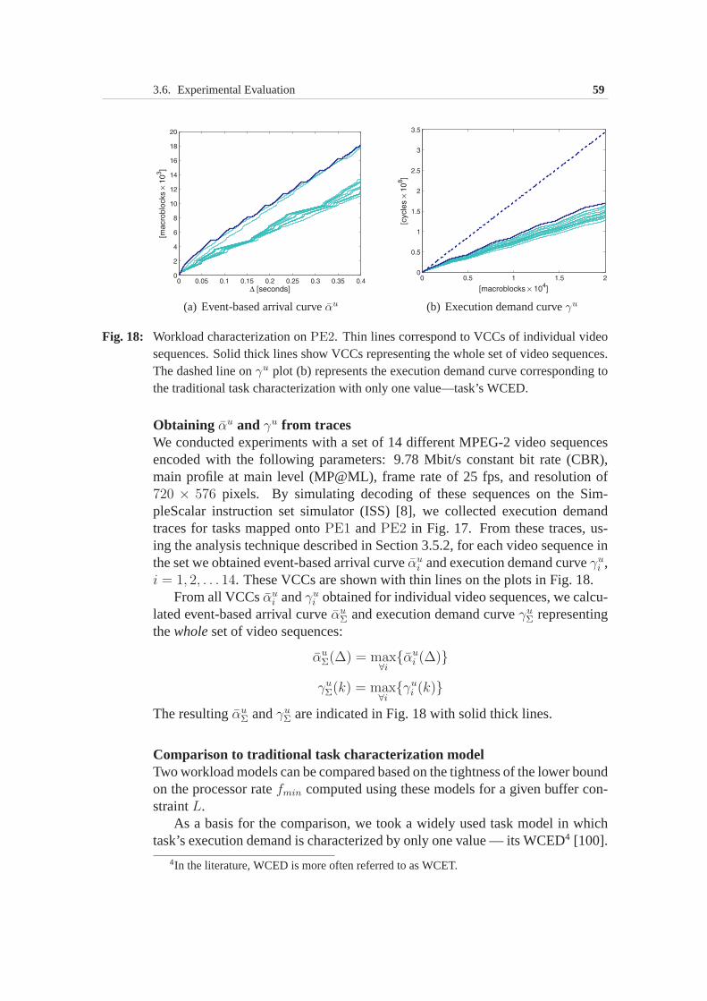
3.6. Experimental Evaluation 59
(a) Event-based arrival curveαu (b) Execution demand curveγu
Fig. 18: Workload characterization onPE2. Thin lines correspond to VCCs of individual videosequences. Solid thick lines show VCCs representing the whole set of video sequences.The dashed line onγu plot (b) represents the execution demand curve corresponding tothe traditional task characterization with only one value—task’s WCED.
Obtaining αu and γu from tracesWe conducted experiments with a set of 14 different MPEG-2 video sequencesencoded with the following parameters: 9.78 Mbit/s constant bit rate (CBR),main profile at main level (MP@ML), frame rate of 25 fps, and resolution of720 × 576 pixels. By simulating decoding of these sequences on the Sim-pleScalar instruction set simulator (ISS) [8], we collected execution demandtraces for tasks mapped ontoPE1 andPE2 in Fig. 17. From these traces, us-ing the analysis technique described in Section 3.5.2, for each video sequence inthe set we obtained event-based arrival curveαu
i and execution demand curveγui ,
i = 1, 2, . . . 14. These VCCs are shown with thin lines on the plots in Fig. 18.From all VCCsαu
i andγui obtained for individual video sequences, we calcu-
lated event-based arrival curveαuΣ and execution demand curveγu
Σ representingthewholeset of video sequences:
αuΣ(∆) = max
∀i{αu
i (∆)}
γuΣ(k) = max
∀i{γu
i (k)}The resultingαu
Σ andγuΣ are indicated in Fig. 18 with solid thick lines.
Comparison to traditional task characterization modelTwo workload models can be compared based on the tightness ofthe lower boundon the processor ratefmin computed using these models for a given buffer con-straintL.
As a basis for the comparison, we took a widely used task modelin whichtask’s execution demand is characterized by only one value —its WCED4 [100].
4In the literature, WCED is more often referred to as WCET.
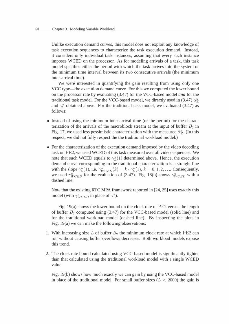
60 Chapter 3. Modeling Variable Workload
Unlike execution demand curves, this model does not exploitany knowledge oftask execution sequences to characterize the task execution demand. Instead,it considers only individual task instances, assuming thatevery such instanceimposes WCED on the processor. As for modeling arrivals of a task, this taskmodel specifies either the period with which the task arrivesinto the system orthe minimum time interval between its two consecutive arrivals (the minimuminter-arrival time).
We were interested in quantifying the gain resulting from using only oneVCC type—the execution demand curve. For this we computed thelower boundon the processor rate by evaluating (3.47) for the VCC-based model and for thetraditional task model. For the VCC-based model, we directly used in (3.47)αu
Σ
andγuΣ obtained above. For the traditional task model, we evaluated (3.47) as
follows:
• Instead of using the minimum inter-arrival time (or the period) for the charac-terization of the arrivals of the macroblock stream at the input of bufferB2 inFig. 17, we used less pessimistic characterization with themeasuredαu
Σ. (In thisrespect, we did not fully respect the the traditional workload model.)
• For the characterization of the execution demand imposed bythe video decodingtask onPE2, we used WCED of this task measured over all video sequences. Wenote that such WCED equals toγu
Σ(1) determined above. Hence, the executiondemand curve corresponding to the traditional characterization is a straight linewith the slopeγu
Σ(1), i.e. γuWCED(k) = k · γu
Σ(1), k = 0, 1, 2, . . .. Consequently,we usedγu
WCED for the evaluation of (3.47). Fig. 18(b) showsγuWCED with a
dashed line.
Note that the existing RTC MPA framework reported in [24, 25]uses exactly thismodel (withγu
WCED in place ofγu).
Fig. 19(a) shows the lower bound on the clock rate ofPE2 versus the lengthof bufferB2 computed using (3.47) for the VCC-based model (solid line) andfor the traditional workload model (dashed line). By inspecting the plots inFig. 19(a) we can make the following observations:
1. With increasing sizeL of bufferB2 the minimum clock rate at whichPE2 canrun without causing buffer overflows decreases. Both workload models exposethis trend.
2. The clock rate bound calculated using VCC-based model is significantly tighterthan that calculated using the traditional workload model with a single WCEDvalue.
Fig. 19(b) shows how much exactly we can gain by using the VCC-based modelin place of the traditional model. For small buffer sizes (L < 2000) the gain is
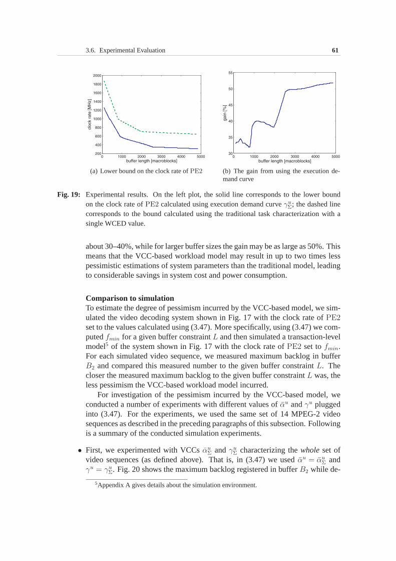
3.6. Experimental Evaluation 61
(a) Lower bound on the clock rate ofPE2 (b) The gain from using the execution de-mand curve
Fig. 19: Experimental results. On the left plot, the solid line corresponds to the lower boundon the clock rate ofPE2 calculated using execution demand curveγu
Σ; the dashed linecorresponds to the bound calculated using the traditional task characterization with asingle WCED value.
about 30–40%, while for larger buffer sizes the gain may be aslarge as 50%. Thismeans that the VCC-based workload model may result in up to two times lesspessimistic estimations of system parameters than the traditional model, leadingto considerable savings in system cost and power consumption.
Comparison to simulationTo estimate the degree of pessimism incurred by the VCC-based model, we sim-ulated the video decoding system shown in Fig. 17 with the clock rate ofPE2set to the values calculated using (3.47). More specifically, using (3.47) we com-putedfmin for a given buffer constraintL and then simulated a transaction-levelmodel5 of the system shown in Fig. 17 with the clock rate ofPE2 set tofmin.For each simulated video sequence, we measured maximum backlog in bufferB2 and compared this measured number to the given buffer constraint L. Thecloser the measured maximum backlog to the given buffer constraintL was, theless pessimism the VCC-based workload model incurred.
For investigation of the pessimism incurred by the VCC-based model, weconducted a number of experiments with different values ofαu andγu pluggedinto (3.47). For the experiments, we used the same set of 14 MPEG-2 videosequences as described in the preceding paragraphs of this subsection. Followingis a summary of the conducted simulation experiments.
• First, we experimented with VCCsαuΣ andγu
Σ characterizing thewholeset ofvideo sequences (as defined above). That is, in (3.47) we usedαu = αu
Σ andγu = γu
Σ. Fig. 20 shows the maximum backlog registered in bufferB2 while de-
5Appendix A gives details about the simulation environment.
62 Chapter 3. Modeling Variable Workload
1 2 3 4 5 6 7 8 9 10 11 12 13 140
0.2
0.4
0.6
0.8
norm
aliz
ed m
ax. b
ackl
og
video sequence #
Buffer size:
250
500
1000
3000
Fig. 20: Normalized maximum backlogs registered in bufferB2 in Fig. 17 when the clock rate ofPE2 was set to the values obtained from the VCC-based model characterizing thewholeset of the MPEG-2 video sequences.
coding different video sequences in the set. The maximum backlog shown inFig. 20 is normalized to buffer constraintL (”buffer size”) for which the corre-spondingfmin was computed. The bar plot in Fig. 20 shows that for all but onevideo sequence (#1) the maximum backlog inB2 was less than half of buffer sizeL. For video sequence #1 and buffer sizesL = {250, 1000, 3000}, the maximumbacklog was about half ofL. However, for buffer sizeL = 500, video sequence#1 causedB2 to be filled up to 80%. Although for the rest of video sequencesthecomputed bound on the clock rate is seemingly pessimistic, given the fact that weperformed worst-case analysis by abstracting thewholeset of video sequenceswith only one pair of VCCs,αu
Σ andγuΣ, we can conclude that the pessimism
incurred by the VCC-based model is relatively low. The simulation results pre-sented in Fig. 20 indicate that sequence #1, probably, imposes a highly burstyworkload onPE2, and represents for the system the most ”adverse” (in termsof the imposed workload) video sequence among all other sequences in the set.VCCs could accurately capture this worst-case.
• To estimate how pessimistic a VCC abstraction of asinglevideo sequence canbe, we conducted a series of experiments in which for computation of the lowerbound on the clock rate ofPE2, we plugged into (3.47) VCCs characterizingindividual video sequences. That is, in (3.47) we usedαu = αu
i andγu = γui ,
wherei = 1, 2, . . . , 14. Thus, for a given buffer sizeL we computed values offmin for each video sequence in the set and simulated decoding of each videosequence with the corresponding to it value offmin. The resulting normalizedmaximum backlogs registered in bufferB2 are depicted in Fig. 21. The simula-tion results in Fig. 21 show that for all video sequences and all buffer sizesL themaximum backlogs inB2 were larger than 50%. Moreover, in Fig. 21 we cansee that in many configurations the buffer was almost full. This indicates that
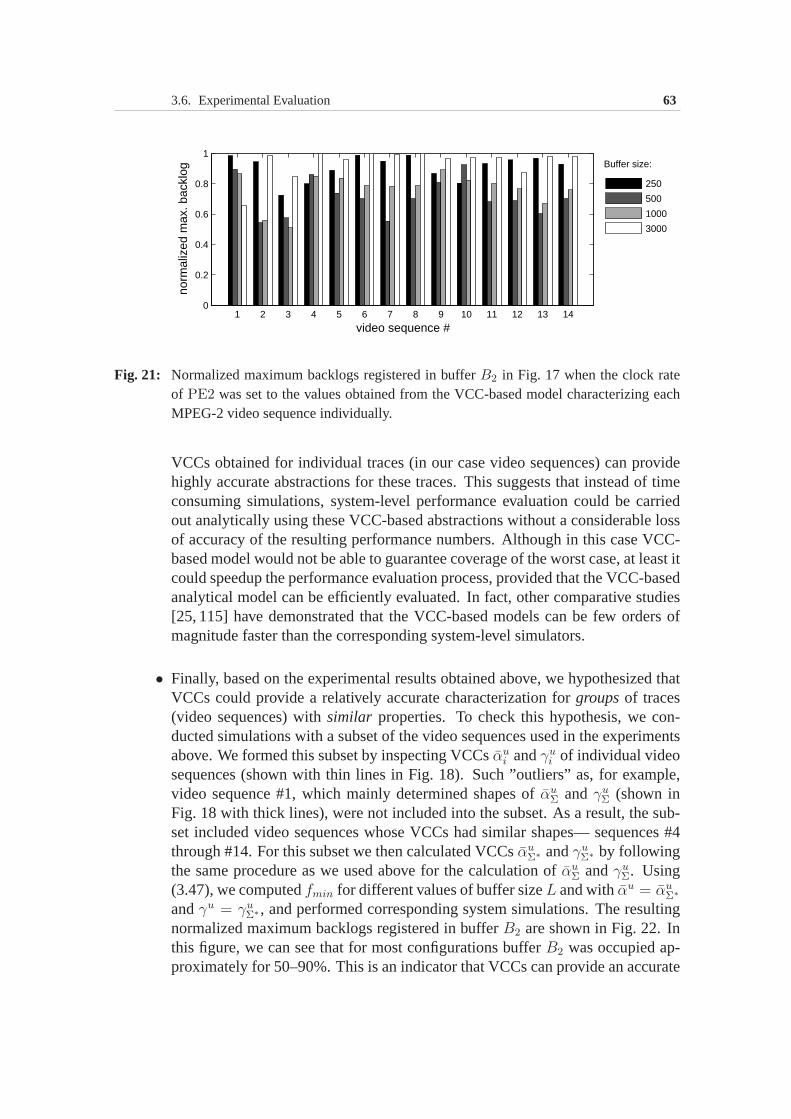
3.6. Experimental Evaluation 63
1 2 3 4 5 6 7 8 9 10 11 12 13 140
0.2
0.4
0.6
0.8
1
norm
aliz
ed m
ax. b
ackl
og
video sequence #
Buffer size:
250
500
1000
3000
Fig. 21: Normalized maximum backlogs registered in bufferB2 in Fig. 17 when the clock rateof PE2 was set to the values obtained from the VCC-based model characterizing eachMPEG-2 video sequence individually.
VCCs obtained for individual traces (in our case video sequences) can providehighly accurate abstractions for these traces. This suggests that instead of timeconsuming simulations, system-level performance evaluation could be carriedout analytically using these VCC-based abstractions withouta considerable lossof accuracy of the resulting performance numbers. Althoughin this case VCC-based model would not be able to guarantee coverage of the worst case, at least itcould speedup the performance evaluation process, provided that the VCC-basedanalytical model can be efficiently evaluated. In fact, other comparative studies[25, 115] have demonstrated that the VCC-based models can be few orders ofmagnitude faster than the corresponding system-level simulators.
• Finally, based on the experimental results obtained above,we hypothesized thatVCCs could provide a relatively accurate characterization for groupsof traces(video sequences) withsimilar properties. To check this hypothesis, we con-ducted simulations with a subset of the video sequences usedin the experimentsabove. We formed this subset by inspecting VCCsαu
i andγui of individual video
sequences (shown with thin lines in Fig. 18). Such ”outliers” as, for example,video sequence #1, which mainly determined shapes ofαu
Σ andγuΣ (shown in
Fig. 18 with thick lines), were not included into the subset.As a result, the sub-set included video sequences whose VCCs had similar shapes— sequences #4through #14. For this subset we then calculated VCCsαu
Σ∗ andγuΣ∗ by following
the same procedure as we used above for the calculation ofαuΣ andγu
Σ. Using(3.47), we computedfmin for different values of buffer sizeL and withαu = αu
Σ∗
andγu = γuΣ∗, and performed corresponding system simulations. The resulting
normalized maximum backlogs registered in bufferB2 are shown in Fig. 22. Inthis figure, we can see that for most configurations bufferB2 was occupied ap-proximately for 50–90%. This is an indicator that VCCs can provide an accurate
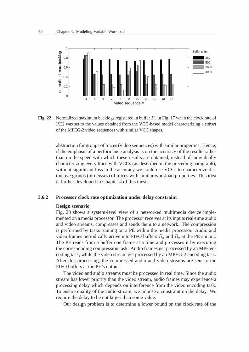
64 Chapter 3. Modeling Variable Workload
4 5 6 7 8 9 10 11 12 13 140
0.2
0.4
0.6
0.8
1
norm
aliz
ed m
ax. b
ackl
og
video sequence #
Buffer size:
250
500
1000
3000
Fig. 22: Normalized maximum backlogs registered in bufferB2 in Fig. 17 when the clock rate ofPE2 was set to the values obtained from the VCC-based model characterizing asubsetof the MPEG-2 video sequences with similar VCC shapes.
abstraction for groups of traces (video sequences) with similar properties. Hence,if the emphasis of a performance analysis is on the accuracy of the results ratherthan on the speed with which these results are obtained, instead of individuallycharacterizing every trace with VCCs (as described in the preceding paragraph),without significant loss in the accuracy we could use VCCs to characterize dis-tinctive groups (orclasses) of traces with similar workload properties. This ideais further developed in Chapter 4 of this thesis.
3.6.2 Processor clock rate optimization under delay constraint
Design scenarioFig. 23 shows a system-level view of a networked multimedia device imple-mented on a media processor. The processor receives at its inputs real-time audioand video streams, compresses and sends them to a network. The compressionis performed by tasks running on a PE within the media processor. Audio andvideo frames periodically arrive into FIFO buffersBa andBv at the PE’s input.The PE reads from a buffer one frame at a time and processes it by executingthe corresponding compression task: Audio frames get processed by an MP3 en-coding task, while the video stream get processed by an MPEG-2 encoding task.After this processing, the compressed audio and video streams are sent to theFIFO buffers at the PE’s output.
The video and audio streams must be processed in real time. Since the audiostream has lower priority than the video stream, audio frames may experience aprocessing delay which depends on interference from the video encoding task.To ensure quality of the audio stream, we impose a constrainton the delay. Werequire the delay to be not larger than some value.
Our design problem is to determine a lower bound on the clock rate of the
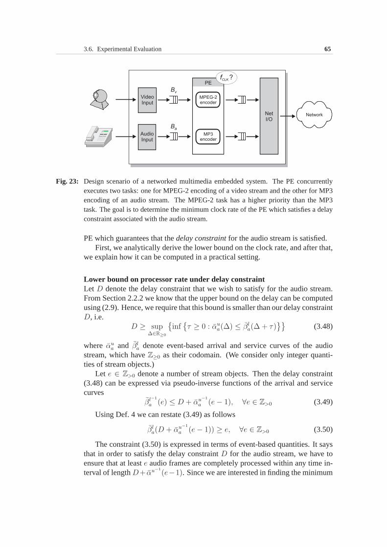
3.6. Experimental Evaluation 65
Fig. 23: Design scenario of a networked multimedia embedded system. The PE concurrentlyexecutes two tasks: one for MPEG-2 encoding of a video stream and the other for MP3encoding of an audio stream. The MPEG-2 task has a higher priority than theMP3task. The goal is to determine the minimum clock rate of the PE which satisfies a delayconstraint associated with the audio stream.
PE which guarantees that thedelay constraintfor the audio stream is satisfied.First, we analytically derive the lower bound on the clock rate, and after that,
we explain how it can be computed in a practical setting.
Lower bound on processor rate under delay constraintLet D denote the delay constraint that we wish to satisfy for the audio stream.From Section 2.2.2 we know that the upper bound on the delay can be computedusing (2.9). Hence, we require that this bound is smaller than our delay constraintD, i.e.
D ≥ sup∆∈R≥0
{
inf{
τ ≥ 0 : αua(∆) ≤ βl
a(∆ + τ)}}
(3.48)
where αua and βl
a denote event-based arrival and service curves of the audiostream, which haveZ≥0 as their codomain. (We consider only integer quanti-ties of stream objects.)
Let e ∈ Z>0 denote a number of stream objects. Then the delay constraint(3.48) can be expressed via pseudo-inverse functions of thearrival and servicecurves
βl−1
a (e) ≤ D + αu−1
a (e− 1), ∀e ∈ Z>0 (3.49)
Using Def. 4 we can restate (3.49) as follows
βla(D + αu−1
a (e− 1)) ≥ e, ∀e ∈ Z>0 (3.50)
The constraint (3.50) is expressed in terms of event-based quantities. It saysthat in order to satisfy the delay constraintD for the audio stream, we have toensure that at leaste audio frames are completely processed within any time in-terval of lengthD+ αu−1
(e−1). Since we are interested in finding the minimum
66 Chapter 3. Modeling Variable Workload
rate of the PE expressed in terms ofclock cycles, we have to apply a workloadtransformation to (3.50). This will give us a constraint on the amount of clockcycles required to satisfy (3.50). For the workload transformation we employ theexecution demand curves of the audio task(γl
a, γua ). Under pessimistic assump-
tions we get
(γla ⊙ βl
a)(D + αu−1
a (e− 1)) ≥ γua ⊙ e, ∀e ∈ Z>0
and using (3.36) we obtain
βla(D + αu−1
a (e− 1)) ≥ γua (e), ∀e ∈ Z>0 (3.51)
The left hand side of (3.51) denotes the required resource-based service curve forthe audio stream, while the right-hand side denotes the upper bound on the num-ber of processor cycles that may be required to completely process any numbere of consecutive audio frames.
From the problem definition we know that the video encoding task has ahigher priority than the audio task. Hence, the video streamcan acquire the fullprocessor capacity, while the audio stream can get only the service which hasbeen left after the processing of the video stream. To find theremaining servicefor the audio stream, we can use (2.4) as follows.
βla(τ) = sup
∀∆∈[0,τ ]
{
βlv(∆) − αu
v(∆)}
∨ 0 (3.52)
whereβlv andαu
v denote the resource-based service and arrival curves of thevideo stream.
Using (3.52) and by noting that the service curve corresponding to the fullprocessor capacity is determined asf · ∆, wheref denotes the processor clockrate, we can restate constraint (3.51) as follows.
sup∀∆∈[0,D+αu−1
a (e−1)]
{f · ∆ − αuv(∆)} ≥ γu
a (e), ∀e ∈ Z>0 (3.53)
To satisfy (3.53) for a given value ofe, it is sufficient to selectf large enoughsuch that there exists∆′ ∈ [0, D + αu−1
a (e− 1)] for which
f(e) · ∆′ ≥ αuv(∆
′) + γua (e)
holds true. Since we are looking for the lower bound on the clock rate we requirethat
f(e) ≥ inf∀∆∈[0,D+αu−1
a (e−1)]
{
αuv(∆) + γu
a (e)
∆
}
, ∀e ∈ Z>0 (3.54)
To ensure that for anye ∈ Z>0 the above constraint is satisfied, we take themaximum value of all possible values off(e).
fmin = sup∀e∈Z>0
{
inf∀∆∈[0,D+αu−1
a (e−1)]
{
αuv(∆) + γu
a (e)
∆
}
}
(3.55)
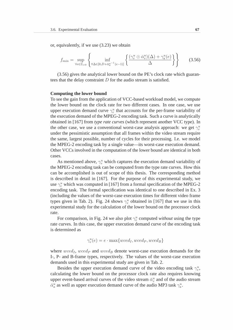
3.6. Experimental Evaluation 67
or, equivalently, if we use (3.23) we obtain
fmin = sup∀e∈Z>0
{
inf∀∆∈[0,D+αu−1
a (e−1)]
{
(γuv ⊙ αu
v)(∆) + γua (e)
∆
}
}
(3.56)
(3.56) gives the analytical lower bound on the PE’s clock rate which guaran-tees that the delay constraintD for the audio stream is satisfied.
Computing the lower boundTo see the gain from the application of VCC-based workload model, we computethe lower bound on the clock rate for two different cases. In one case, we useupper execution demand curveγu
v that accounts for the per-frame variability ofthe execution demand of the MPEG-2 encoding task. Such a curve is analyticallyobtained in [167] fromtype rate curves(which represent another VCC type). Inthe other case, we use a conventional worst-case analysis approach: we getγu
v
under the pessimistic assumption that all frames within thevideo stream requirethe same, largest possible, number of cycles for their processing. I.e. we modelthe MPEG-2 encoding task by a single value—its worst-case execution demand.Other VCCs involved in the computation of the lower bound are identical in bothcases.
As mentioned above,γuv which captures the execution demand variability of
the MPEG-2 encoding task can be computed from the type rate curves. How thiscan be accomplished is out of scope of this thesis. The corresponding methodis described in detail in [167]. For the purpose of this experimental study, weuseγu
v which was computed in [167] from a formal specification of theMPEG-2encoding task. The formal specification was identical to onedescribed in Ex. 3(including the values of the worst-case execution times fordifferent video frametypes given in Tab. 2). Fig. 24 showsγu
v obtained in [167] that we use in thisexperimental study for the calculation of the lower bound onthe processor clockrate.
For comparison, in Fig. 24 we also plotγuv computedwithoutusing the type
rate curves. In this case, the upper execution demand curve of the encoding taskis determined as
γuv (e) = e · max{wcedI , wcedP , wcedB}
wherewcedI , wcedP andwcedB denote worst-case execution demands for theI-, P- and B-frame types, respectively. The values of the worst-case executiondemands used in this experimental study are given in Tab. 2.
Besides the upper execution demand curve of the video encoding taskγuv ,
calculating the lower bound on the processor clock rate alsorequires knowingupper event-based arrival curves of the video streamαu
v and of the audio streamαu
a as well as upper execution demand curve of the audio MP3 taskγua .
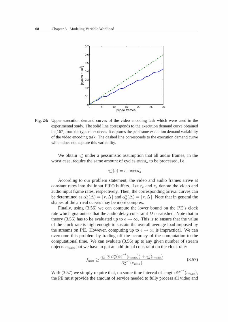
68 Chapter 3. Modeling Variable Workload
0 5 10 15 20 25 300
0.1
0.2
0.3
0.4
0.5
0.6
0.7
[video frames]
[cyc
les
× 10
9 ]
Fig. 24: Upper execution demand curves of the video encoding task which were used in theexperimental study. The solid line corresponds to the execution demand curve obtainedin [167] from the type rate curves. It captures the per-frame executiondemand variabilityof the video encoding task. The dashed line corresponds to the executiondemand curvewhich does not capture this variability.
We obtainγua under a pessimistic assumption that all audio frames, in the
worst case, require the same amount of cycleswceda to be processed, i.e.
γua (e) = e · wceda
According to our problem statement, the video and audio frames arrive atconstant rates into the input FIFO buffers. Letrv andra denote the video andaudio input frame rates, respectively. Then, the corresponding arrival curves canbe determined asαu
v(∆) = ⌈rv∆⌉ andαua(∆) = ⌈ra∆⌉. Note that in general the
shapes of the arrival curves may be more complex.Finally, using (3.56) we can compute the lower bound on thePE’s clock
rate which guarantees that the audio delay constraintD is satisfied. Note that intheory (3.56) has to be evaluated up toe→ ∞. This is to ensure that the valueof the clock rate is high enough to sustain the overall average load imposed bythe streams onPE. However, computing up toe→ ∞ is impractical. We canovercome this problem by trading off the accuracy of the computation to thecomputational time. We can evaluate (3.56) up to any given number of streamobjectsemax, but we have to put an additional constraint on the clock rate:
fmin ≥ γuv ⊙ αu
v(αu−1
a (emax)) + γua (emax)
αu−1
a (emax)(3.57)
With (3.57) we simply require that, on some time interval of lengthαu−1
a (emax),the PE must provide the amount of service needed to fully process all video and
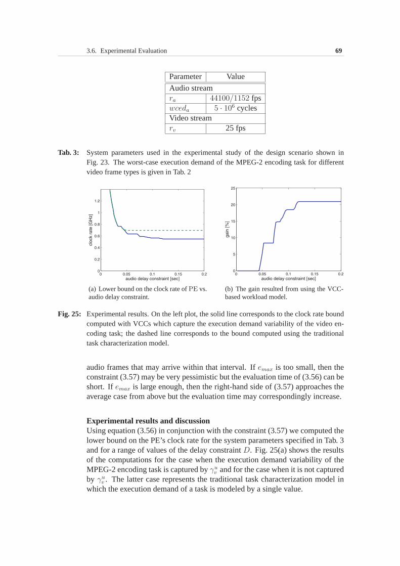
3.6. Experimental Evaluation 69
Parameter Value
Audio streamra 44100/1152 fpswceda 5 · 106 cyclesVideo streamrv 25 fps
Tab. 3: System parameters used in the experimental study of the design scenario shown inFig. 23. The worst-case execution demand of the MPEG-2 encoding task for differentvideo frame types is given in Tab. 2
(a) Lower bound on the clock rate ofPE vs.audio delay constraint.
(b) The gain resulted from using the VCC-based workload model.
Fig. 25: Experimental results. On the left plot, the solid line corresponds to the clock rate boundcomputed with VCCs which capture the execution demand variability of the video en-coding task; the dashed line corresponds to the bound computed using the traditionaltask characterization model.
audio frames that may arrive within that interval. Ifemax is too small, then theconstraint (3.57) may be very pessimistic but the evaluation time of (3.56) can beshort. Ifemax is large enough, then the right-hand side of (3.57) approaches theaverage case from above but the evaluation time may correspondingly increase.
Experimental results and discussionUsing equation (3.56) in conjunction with the constraint (3.57) we computed thelower bound on the PE’s clock rate for the system parameters specified in Tab. 3and for a range of values of the delay constraintD. Fig. 25(a) shows the resultsof the computations for the case when the execution demand variability of theMPEG-2 encoding task is captured byγu
v and for the case when it is not capturedby γu
v . The latter case represents the traditional task characterization model inwhich the execution demand of a task is modeled by a single value.
70 Chapter 3. Modeling Variable Workload
In Fig. 25(b), we plot the gain resulted from the usage of the VCC-basedworkload model. For different values of the audio delay constraint, the plotshows the percentage by which the lower bound on the clock rate computed us-ing γu
v that captures the execution demand variability of the videotask is smallerthan the corresponding bound computed usingγu
v that does not capture this vari-ability (i.e. which was obtained under the assumption that all video frames havethe same execution requirement in the worst case). By inspecting the plot inFig. 25(b), we can see that for large values of the delay constraint we can gain upto 20% of savings in the clock rate by capturing the workload variability usingVCCs.
3.7 SummaryIn this chapter, we presented two central to this thesis concepts —VariabilityCharacterization CurvesandWorkload Transformations. We discussed differentways to obtaining VCCs and defined several VCC types for modelingmulti-media workloads. We also proposed and justified the optimal placement of theworkload transformations in an MPA scheduling network. Finally, we presentedresults of an experimental evaluation of the VCC-based workload model. Ourexperiments showed that the VCC-based model results in significantly tighteranalytic bounds than a traditional model. The simulation study suggested thatthese bounds represent useful estimates of system properties and therefore canserve as a sound basis for making design decisions. In this simulation studywe also investigated the effect of grouping the traces for obtaining VCCs on thetightness of the analytic bounds. We came to the conclusion that in certain de-sign contexts it might be of advantage to distinguish between different workloadclasses.
In the rest of this thesis, we demonstrate the utility of the VCC-based work-load model and of the workload transformations in differentdesign contexts ofmultimedia MpSoC architectures. In particular, in the nextchapter we further ex-plore the idea of distinguishing between different workload classes: we employVCCs for automatic exploration of theworkloaddesign space.
4Workload Design
Chapter 3 introduced the concept of Variability Characterization Curves (VCCs)and demonstrated how they can capture different propertiesof multimedia work-loads. This chapter shows how VCCs can help to address an emerging and chal-lenging problem ofworkload designfor system-level performance evaluation ofmultimedia MpSoC architectures.
“Workload design” refers to a process of selecting representative workloadfor performance evaluation and comparison of computer architectures [39]. Itis a well recognized problem in the domain of microprocessordesign. In thisdomain, different program characteristics that influence the selection of a rep-resentative workload include microarchitecture-centricproperties such as cachemiss rates, instruction mix and accuracy of branch prediction. However, work-load properties that are pertinent to the context of system-level design of multi-processor SoC architectures are very different. To date theproblem of workloaddesign, in this specific context, has not been sufficiently addressed. This chap-ter presents results appeared in [114], which suggests how this problem can beapproached in the specific case of media processor design. This chapter has thefollowing structure:
• Section 4.1 introduces and motivates the problem of workload design for system-level performance evaluation of multiprocessor SoC platform architectures.
• Section 4.2 summarizes relevant research work.
• Section 4.3 outlines the proposed approach.
• Section 4.4 proposes VCCs as a basis for workload characterization necessaryfor quantitative comparison and classification of media streams.
72 Chapter 4. Workload Design
• Section 4.5 describes how various media streams can be classified based onVCCs characterizing them.
• Section 4.6 presents results of an empirical validation of the proposed workloadclassification method.
• Finally, Section 4.7 concludes this chapter.
4.1 IntroductionA typical design process of a complex embedded system such asa multimediaMpSoC platform involves a thorough exploration of the available design space.Starting from some template architecture — the platform, system designers it-eratively evolve this platform with the goal to arrive at an architecture whichwould be optimal for the target application range. Searching for the optimal ar-chitecture necessitates evaluating and comparing to each other many alternativeplatform configurations. Traditionally, performance evaluation of architecturesheavily relies on simulations. For system designers to be sure in representa-tiveness of performance numbers obtained from such simulations, ideally, eachcandidate architecture needs to be simulated for a large anddiverse set of possi-ble inputs (or application scenarios). However, in most cases this is impractical.This is because simulating a single design point may be prohibitively expensivein terms of the simulation time. For example, simulation of only a few minutesof video, for a video decoding application, may take tens of hours [165]. Thissignificantly limits the number of different inputs for which simulations can beperformed within an allotted design time. Therefore, from the large set of pos-sible inputs, the system designers have to choose a small subset which wouldbe representative1 of the workload that the system would experience in reality.Simulations can then be restricted to this subset only.
Obtaining a representative input set is, of course, not a newconcern—workloaddesign and other relevant problems, such as workload characterization, bench-mark construction, synthetic workload generation, etc., are well recognized prob-lems in different areas of computer performance evaluation. However, issuesinvolved in solving these problems are almost always domain-specific. This isbecause they depend on the nature of applications and architectures, and on theabstraction level at which systems are evaluated. For example, the main issues
1Many sources in the literature refer to “representative workload” as the workload (e.g. a col-lection of traces) which represents arealisticgeneral case, and is not biased towards a particulararchitecture, environment, etc. This term is often used in conjunction with asynthetic workload,to indicate that the synthetic workload closely resembles the real workload. In context of thisthesis, we use the term “representative workload” in a slightly different way. By “representativeworkload” we mean a workload which was selected from a largercollection of real workloads,such that it best represents (covers) all important classes of the workload within this collection.
4.1. Introduction 73
in the domain of microprocessor design are microarchitecture-centric, where adesigner is mostly concerned with program characteristicslike instruction mix,data and instruction cache miss rates and branch predictionaccuracy. On theother hand, the concerns in the case of system-level design of SoC platform ar-chitectures are very different and these are not suitably reflected in a benchmarksuite designed for microarchitecture evaluation.
In this chapter, we attempt to address this issue of workloaddesign in thespecific context of system-level design of SoC platform architectures for multi-media processing (i.e. media processors). Although simulation-oriented designand evaluation are widespread in the domain of system-levelSoC design, to thebest of our knowledge the issue of methodically selecting representative inputsfor architecture evaluation has not received any attentionso far. Most of the workreported in the Embedded Systems literature, on novel system models or simu-lation schemes, shirk off this problem and leave the responsibility of choosing arepresentative input or stimuli to the architecture on system designers (see, forexample, [83]).
There are many reasons why this problem is interesting in thespecific caseof multimedia processing on multiprocessor SoC platforms.First, media streamsmay impose very complex and diverse workloads on such platforms. Manymultimedia applications exhibit a large degree of data-dependent variability thatcomplicates the problem of choosing a representative inputset. Second, in con-trast to general-purpose architectures, MpSoC platforms,which are optimizedfor stream processing, have heterogeneous distributed architectures. This factfurther complicates the problem. Third, multimedia processing is in generalcomputationally intensive, requiring for performance evaluation to simulate arelatively large number of events. This makes selection of the representativeworkload for design of media processors an important problem.
Arbitrarily selecting inputs to form the “representative”input set is certainlynot a good idea. The goal of “representative” workload design should be to se-lect inputs such that they cover, as much as possible, the whole space of possibleworkloads, including those that representcorner casesfor the target architecture.Such corner cases are represented by inputs which impose worst- and best-caseloads on different parts of the architecture. Determining what constitutes a “cor-ner case” is, however, not a trivial undertaking due to the complex nature ofmost multimedia workloads. Attempts towards using somequalitative(i.e. sub-jective) technique to judge the properties of media streamsbased on their content(for example, by simply viewing video clips to be processed by the architectureand classifying them based on experience or intuition) might easily fail. Hence,a quantitative methodology is necessary, using which it should be possible toobjectively assess and compare the properties of differentmedia streams. Basedon such a comparison, a smallrepresentativesubset can then be chosen from alarge collection of samples.
We propose a methodology to classify media streams which canbe used to
74 Chapter 4. Workload Design
identify a small representative set meant for architectureevaluation. Towardsthis, we first hypothesize that key characteristics of mediastreams that influencethe performance of an MpSoC platform architecture, are related to their “vari-ability”. This variability stem from the fact that execution time requirements ofmultimedia tasks and the amount of data consumed (produced)by these tasksat their inputs (outputs) depend on the properties of particular audio/video sam-ples being processed. Now, given a collection of media streams, we classifytwo streams from this collection assimilar if both of them exhibit the same kindof variability with respect to the execution time requirements and the task in-put/output rates, as mentioned above. Therefore, given a set of video streamswhich aresimilar, it would be sufficient to simulate an architecture with onlyone video stream from this set, as all the other streams wouldimpose similarload on the architecture. To quantitatively characterize the variability associatedwith a stream, with respect to a given architecture, we use the concept of VCCs,introduced in Chapter 3. As an illustration of our methodology, throughout thischapter we use a case study of an MPEG-2 decoder system whose system-levelarchitecture, including the mapping of MPEG-2 tasks onto it, is shown in Fig. 17and described in Section 3.6.1.
We would like to point out here that the kinds of variabilities that should beconsidered in a media stream for an effective classificationwould depend on theplatform architecture and the application at hand. This is mainly due to the factthat SoC architectures are often highly specialized for a narrow application spec-trum. For this reason, defining a set of workload attributes which would result inan effective stream classification inanydesign scenario is difficult, if not impos-sible. Also, we note that defining a common benchmark for multimedia MpSoCplatforms is out of scope of this chapter. The contribution of this chapter is topoint out that the properties of media streams which should be considered forrepresentative workload identification in the context of performance evaluationof multimedia MpSoC platforms can be expressed in the form ofVCCs, and topropose the corresponding stream classification method.
Finally, we note that, in a system-level design framework, the selection ofthe representative workload can be carried out outside of the time-critical designspace exploration loop (namely, prior to the exploration) and does not requiretime-consuming system simulations. Furthermore, the workload characteriza-tion and classification procedures presented in this chapter can be fully auto-mated, reducing to minimum designers’ participation in theworkload selectionprocess.
4.2 Related WorkThe construction of representative workloads for performance evaluation of com-puter systems has always been an area of active research since early 70s (see
4.3. Overview 75
[148] and references therein). Since then the termworkload has been widelyunderstood as a mix of programs (or jobs, or applications) for which the perfor-mance of a computer system was evaluated. Domain-specific collections of suchprograms, calledbenchmarks, have been designed and widely used as a stan-dard means to evaluate and compare computer architectures.Examples of these,in the multimedia domain, are MediaBench [86] and the Berkeleymultimediaworkload [146]. Design of such representative workloads was mainly concen-trated on proper selection of theprogramsto be included in the workload. Theselection of corresponding input data sets was limited to the definition of theirsize (e.g. sampling rate, resolution etc.) The dependency of program behavioron the values of the input data sets did not receive enough consideration in theprocess of forming such representative workloads.
Recently Eeckhout et al. [39] have shown that theworkload design spacemay be very complex and therefore should be systematically explored duringthe construction of representative workloads. Their workload design space con-sists ofprogram-input pairsthat capture both, the variety of programs as wellas various input data sets to those programs. They use techniques such as prin-ciple component analysis and cluster analysis to efficiently explore the space ofpossible workloads and select representative program-input pairs from it.
The problem of reducing simulation time has been addressed using tracesampling techniques(see [82] and references therein). The goal of such tech-niques is to identify representative fragments in the program execution and sim-ulate only those fragments, thereby eliminating the need for simulating the en-tire program. Trace sampling techniques heavily rely on thecharacterization andclassification of the workload imposed on the architecture by the different frag-ments in the program execution trace. However, it should be noted that all theabove mentioned research efforts were primarily targeted towards characteriza-tion and composition of representative workloads in the domain of microproces-sor design.
4.3 OverviewWe assume that system designers have at their disposal a large collection of me-dia streams that fully represents streams which the designed system may haveto process in reality. Then, forming a representative workload from this largecollection involves several steps:
1. Identifying key workload properties: The first step in the workload design isto decide which workload properties are important for the given design context.Based on these properties the workload classification will becarried out. Inthe case of performance evaluation, we have to select those properties that havelargest influence on the performance of the architecture.
76 Chapter 4. Workload Design
2. Characterizing media streams:The next step is to characterize each stream inthe collection. It is accomplished by measuring the properties upon which theworkload classification will be performed. We refer to this step, together withthe preceding step, asworkload characterization.
3. Defining the dissimilarity metric: Based on the workload characterization, weneed to define how the dissimilarity between two workloads (media streams)will be measured. That is, we need to define ametric that would represent thedissimilarity between a pair of media streams as a value. After all media streamsin the collection have been characterized (i.e. their relevant properties have beenmeasured), we compute this metric for each pair of streams inthe collection.
4. Classifying media streams: Having computed the pairwise dissimilarity be-tween the streams in the collection, we can identify groups of streams that mayimpose similar workload on the architecture. Such a group would consists ofstreams that have similar properties. From these groups, wecan then select rep-resentatives. They will form the representative workload for our architecture.We refer to this step and the preceding step asworkload classification.
The next two sections describe particular considerations that we made while re-alizing the above steps.
4.4 Workload CharacterizationWorkload characterization should be based onkey propertiesthat are importantin a particular design context. These are properties that have a strong impact onthe performance of the architecture being designed. For instance, in microar-chitectural design such properties would be instruction mix, branch predictionaccuracy and cache miss rates [39]. As mentioned in Section 4.1, our hypothesisis thaton the system levelthe performance of multimedia MpSoC architecturesis largely influenced by various kinds ofdata-dependent variabilityassociatedwith the processing of media streams. This hypothesis restson the observationthat such variability is the major source of the burstiness of on-chip traffic in suchmultimedia MpSoC platforms [165]. The burstiness of the on-chip traffic neces-sitates insertion of additional buffers between architectural entities processingthe media streams, and deployment of sophisticated scheduling policies acrossthe platform. Both of these inevitably translate into increased design costs andpower consumption [57].
Individual media streams withidentical parameters, such as bit rate, framerate and resolution, may impose significantlydifferent workload on the archi-tecture; in particular, the streams may exhibit different kinds of the variability.This phenomenon can be explained by the fact that, although these streams haveidentical parameters, they contain diverse multimedia information and may have
4.4. Workload Characterization 77
different structure (e.g., in MPEG video streams, different frame types may bearranged in various patterns). For MPEG-2 video streams, this fact is supportedby our experiments reported in Section 4.6. [57] demonstrates the variabilityin streams of several other multimedia formats. Therefore,in the system-leveldesign context of multimedia MpSoC architectures, it is certainly meaningful tocharacterize and classify multimedia workloads with respect to their variabilityproperties.
In a typical MpSoC architecture, consisting of a heterogeneous collection ofinterconnected PEs, often there are several sources of variability that dependson properties of the processed media streams. Consider, as anexample, theMPEG-2 decoding system shown in Fig. 17 in Chapter 3. The system consistsof two programmable processors,PE1 andPE2, and input and output interfaces.PE1 executes a task performing VLD and IQ functions, whereasPE2 executesa task performing IDCT and MC functions of the MPEG-2 decodingalgorithm.For brevity, we will refer to these tasks as VLD and IDCT, respectively. InFig. 17, stream objects belonging to the input stream emerging from the networkinterface are single bits. Stream objects sent fromPE1 to PE2 are partiallydecoded macroblocks, whereas stream objects entering the video interface arefully processed macroblocks. What are the sources of variability associated withmedia streams processed on such an MpSoC platform?
• First, arrival patterns of media streams at the input of the system may have abursty nature, i.e. stream objects may arrive at the system’s input in highly irreg-ular intervals. A typical example of this is a multimedia device receiving streamsfrom a congested network.
• Second, each activation of a task may consume and produce a variable numberof stream objects from the associated streams. For example,each activation ofVLD in Fig. 17 consumes a variable number of bits from the network interface,although it always produces one macroblock at its output.
• Third, the execution demand of a task may vary from activation to activation dueto data-dependent program flow. Both the tasks in our running example of theMPEG-2 decoder—VLD and IDCT—possess this property.
• Finally, stream objects belonging to the same stream may require different amountsof memory to store them in communication channels between PEs. Again, in theexample architecture in Fig. 17, we note that the partially decoded macroblocksstored in bufferB2, depending on their type, may or may not include motionvectors.
All these types of variability must be carefully consideredand characterized dur-ing the workload design process. In this chapter, we will be concerned with thevariability of the execution demand and the consumption andproduction rates oftasks. As mentioned before, depending on the architecture and the application
78 Chapter 4. Workload Design
at hand, it might be meaningful to consider other types of variabilities as well.2
However, we show that the two variability types we consider here already leadto meaningful results.
We propose to use VCCs introduced in Section 3.2 as a model for the work-load characterization that can capture different kinds of variability in mediastreams. To each streami in a stream collection, we associate a set of tuplesSi = {(V l
P ,VuP)}, whereV l
P andVuP denote lower and upper VCCs characteriz-
ing variability of propertyP in streami. For anyP, V lP andVu
P must representthetightest upper and lower VCCs, as defined by Defs. 14 and 15. To obtain suchtightestV l
P andVuP , we use (3.42) and (3.43) under the condition that thefunction
setfor which the VCCs are calculated contains only one function—the functionwhich corresponds to propertyP of the stream being characterized. Thus, theresulting VCCs,V l
P andVuP , representtightestbounds on the worst- and best-
case variability of propertyP in a singlestream. The set of all such VCCs,Si,represents a complete characterization of streami. As a result, in form ofSi, wehave an accurate, compact and easy-to-obtain abstraction of streami.
In Section 3.3, we defined some VCC types useful for multimediaworkloadcharacterization. Out of them, for the workload design in this chapter, we use theexecution demand curves and the consumption and productioncurves, denotedby tuples(γl, γu), (κl, κu), and(πl, πu), respectively. Each task in a multimediastream-processing application is characterized by these VCC types.
We note that(γl, γu) depends on the PE type on which the corresponding ap-plication task is to be executed. For example, if a PE has an application specificinstruction set which may significantly alter the executiondemand of tasks, thenthis will be reflected in(γl, γu). In contrast,(κl, κu) and(πl, πu) are not depen-dent on the architecture, but on the dataflow properties within the application.Hence, the assumption here is that, prior to the workload characterization, weneed to know the partitioning of the application into tasks and the mapping ofthose tasks onto PE types. We believe that this assumption isnot too restrictive.Similar assumptions are common in the Embedded Systems design community,where applications are modeled by task graphs in which the (worst-case) exe-cution demands of tasks are known. In fact, thesameassumption is made in anumber of trace-based performance evaluation techniques recently reported inthe literature [74, 75, 83, 116]. These trace-based performance evaluation tech-niques rely on pre-collected execution traces of tasks on PEs of the MpSoC plat-form being evaluated. Our method can be useful especially inthis context, byproviding such techniques with the representative set of traces.
2It might be also necessary to account for correlations existing between different variabilitytypes. However, this question goes beyond the scope of this chapter.
4.5. Workload Classification 79
4.5 Workload Classification
In the previous section, we described how media streams can be quantitativelycharacterized to enable their comparison and classification. In this section, weexplainhowsuch a comparison and classification can be accomplished based onthis characterization.
We propose to classify streams based on theshapesof the VCCs associatedwith them. If two streams are characterized by VCCs having similar shapes,then their behavior, in the worst/best-case, will also be similar. Each streammight be associated with several VCC types, characterizing different aspects ofvariability within the stream. Therefore, if two streams have similarly shapedVCCs of respective types, then these streams will impose similar workload on thearchitecture (in the worst- and best-case). For example, the maximum backlogsthat such streams will create in the buffers of the architecture as a result of theirprocessing will almost be the same.
4.5.1 Dissimilarity based on a single VCC type
Let us first define a metric that would allow to compare two streams based ononly one VCC type. This metric should be a measure ofdissimilarity betweenshapes of two VCCs of the same type.
In general, any measure of dissimilarity between two objects depends on thespecific problem at hand [45]. Each property, based on which two objects are tobe compared, is associated with a variable. That is, if therearen properties uponwhich two objects have to be compared, then there will ben variables describingeach object. Any valuation of these variables constitutes arepresentation of anobject. The dissimilarity between two objects is then foundby computing somemetric defined over thesen variables. In our case, a VCC, which is defined for aset of pointsk = 1, 2, .., n, can be seen as an object described byn variables.
Intuitively, to see how dissimilar the shapes of two VCCs are, we need tocompare their values for each of the pointsk = 1, 2, .., n. By noting that alln variables represent a VCC along essentiallyseparabledimensions, we canquantitatively measure the dissimilarity between two VCCs using the City Blockmetric [45]. We decided to use this metric as a measure of dissimilarity, because,in comparison to other known metrics (e.g. Euclidean Distance), it is more “sen-sitive” to differences in each of the dimensions (variables). I.e., in our case, themetric is more “sensitive” to the differences in the shapes of two VCCs. A for-mal definition of the dissimilarity between two VCCs based on the City Blockmetric is given below.
Let Vri (k), k = 1, 2, .., n, denote a VCC of typer associated with stream
i. The measure of the pairwise dissimilarity between two streamsi andj, with
80 Chapter 4. Workload Design
respect to VCCVr, is then defined as
drij =n
∑
k=1
ωr(k) |Vri (k) − Vr
j (k)| (4.1)
whereωr(k) = 1/k are weights that are necessary to normalize the differences|Vr
i (k) − Vrj (k)| with respect to the lengthk of the analysis interval. The longer
the analysis intervalk is, the lesscritical the difference in the values of the twoVCCs becomes. For example, suppose that we want to compare upper executiondemand curves of two streams. Assume from the execution demand curves weknow that any two consecutive stream objects (i.e.k = 2) in the first streammay cause a maximum execution demand of 100 units, while for the secondstream this value is 150. Suppose that we also know that any 10consecutivestream objects (k = 10) in the first stream may cause a maximum executiondemand of 1000 units, and it is 1150 units for the second stream. Although theabsolute difference between the curves fork = 2 is smaller than that fork = 10,the difference in the execution demand computedper stream objectfor k = 2is larger than fork = 10 ( |100−150|
2> |1000−1150|
10). For k = 10 the absolute
difference isdistributedover a larger number of stream objects than in the caseof k = 2, and therefore this difference becomes less critical. The weightsωr
allow to correctly compare the streams for largek, e.g. to properly account forlong-term average execution demands.
4.5.2 Dissimilarity based on several VCC types
Media streams may be characterized by more than one VCC type. How can thedissimilarity between the streams be quantified then?
First, we propose to compute the dissimilarities between VCCsof identicaltypes as defined by (4.1). Then, the computed “single-type” dissimilarities canbe combined in a variety of ways. One possibility is to simplysum up all ofthem. Our experiments showed that this simple approach works relatively good.Hence, we define the pairwise dissimilarity between two streamsi andj withrespect to VCCs of typesr ∈ R as [114]
dij =∑
∀r∈R
drij (4.2)
An improved version of (4.2) sums upnormalizeddissimilarities drij
max∀i,j drij, i.e.
dij =∑
∀r∈R
drij
max∀i,j drij
(4.3)
4.5.3 Clustering
Finally, toclassifystreams using the dissimilarity measures described above,weemploy a conventional hierarchical clustering algorithm which uses thecomplete
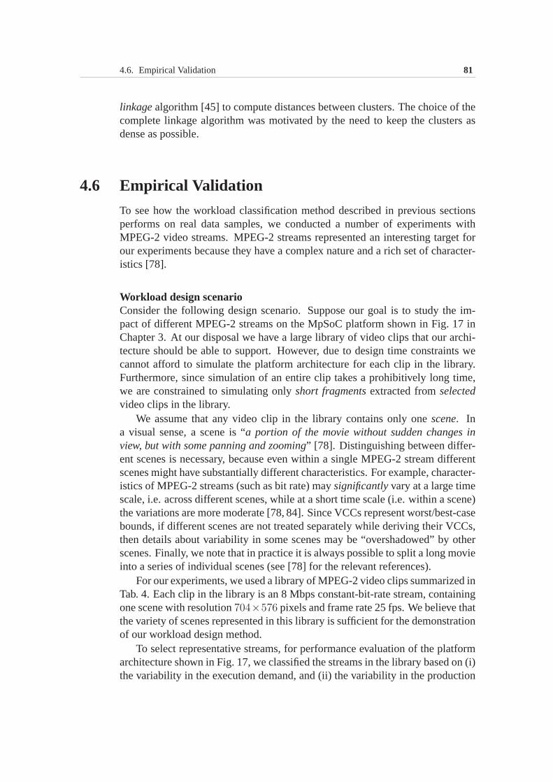
4.6. Empirical Validation 81
linkagealgorithm [45] to compute distances between clusters. The choice of thecomplete linkage algorithm was motivated by the need to keepthe clusters asdense as possible.
4.6 Empirical Validation
To see how the workload classification method described in previous sectionsperforms on real data samples, we conducted a number of experiments withMPEG-2 video streams. MPEG-2 streams represented an interesting target forour experiments because they have a complex nature and a richset of character-istics [78].
Workload design scenarioConsider the following design scenario. Suppose our goal is to study the im-pact of different MPEG-2 streams on the MpSoC platform shownin Fig. 17 inChapter 3. At our disposal we have a large library of video clips that our archi-tecture should be able to support. However, due to design time constraints wecannot afford to simulate the platform architecture for each clip in the library.Furthermore, since simulation of an entire clip takes a prohibitively long time,we are constrained to simulating onlyshort fragmentsextracted fromselectedvideo clips in the library.
We assume that any video clip in the library contains only onescene. Ina visual sense, a scene is “a portion of the movie without sudden changes inview, but with some panning and zooming” [78]. Distinguishing between differ-ent scenes is necessary, because even within a single MPEG-2stream differentscenes might have substantially different characteristics. For example, character-istics of MPEG-2 streams (such as bit rate) maysignificantlyvary at a large timescale, i.e. across different scenes, while at a short time scale (i.e. within a scene)the variations are more moderate [78, 84]. Since VCCs represent worst/best-casebounds, if different scenes are not treated separately while deriving their VCCs,then details about variability in some scenes may be “overshadowed” by otherscenes. Finally, we note that in practice it is always possible to split a long movieinto a series of individual scenes (see [78] for the relevantreferences).
For our experiments, we used a library of MPEG-2 video clips summarized inTab. 4. Each clip in the library is an 8 Mbps constant-bit-rate stream, containingone scene with resolution704×576 pixels and frame rate 25 fps. We believe thatthe variety of scenes represented in this library is sufficient for the demonstrationof our workload design method.
To select representative streams, for performance evaluation of the platformarchitecture shown in Fig. 17, we classified the streams in the library based on (i)the variability in the execution demand, and (ii) the variability in the production
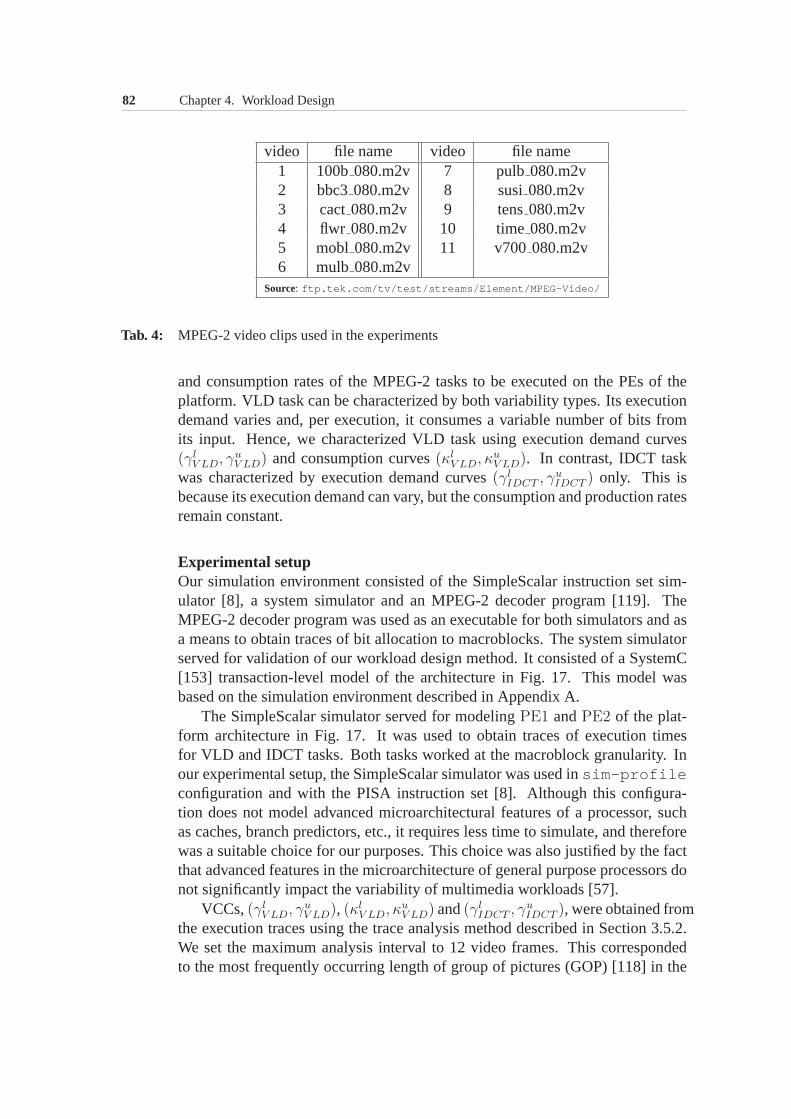
82 Chapter 4. Workload Design
video file name video file name1 100b080.m2v 7 pulb 080.m2v2 bbc3080.m2v 8 susi080.m2v3 cact080.m2v 9 tens080.m2v4 flwr 080.m2v 10 time 080.m2v5 mobl 080.m2v 11 v700 080.m2v6 mulb 080.m2v
Source: ftp.tek.com/tv/test/streams/Element/MPEG-Video/
Tab. 4: MPEG-2 video clips used in the experiments
and consumption rates of the MPEG-2 tasks to be executed on the PEs of theplatform. VLD task can be characterized by both variabilitytypes. Its executiondemand varies and, per execution, it consumes a variable number of bits fromits input. Hence, we characterized VLD task using executiondemand curves(γl
V LD, γuV LD) and consumption curves(κl
V LD, κuV LD). In contrast, IDCT task
was characterized by execution demand curves(γlIDCT , γ
uIDCT ) only. This is
because its execution demand can vary, but the consumption and production ratesremain constant.
Experimental setupOur simulation environment consisted of the SimpleScalar instruction set sim-ulator [8], a system simulator and an MPEG-2 decoder program[119]. TheMPEG-2 decoder program was used as an executable for both simulators and asa means to obtain traces of bit allocation to macroblocks. The system simulatorserved for validation of our workload design method. It consisted of a SystemC[153] transaction-level model of the architecture in Fig. 17. This model wasbased on the simulation environment described in Appendix A.
The SimpleScalar simulator served for modelingPE1 andPE2 of the plat-form architecture in Fig. 17. It was used to obtain traces of execution timesfor VLD and IDCT tasks. Both tasks worked at the macroblock granularity. Inour experimental setup, the SimpleScalar simulator was used insim-profileconfiguration and with the PISA instruction set [8]. Although this configura-tion does not model advanced microarchitectural features of a processor, suchas caches, branch predictors, etc., it requires less time tosimulate, and thereforewas a suitable choice for our purposes. This choice was also justified by the factthat advanced features in the microarchitecture of generalpurpose processors donot significantly impact the variability of multimedia workloads [57].
VCCs,(γlV LD, γ
uV LD), (κl
V LD, κuV LD) and(γl
IDCT , γuIDCT ), were obtained from
the execution traces using the trace analysis method described in Section 3.5.2.We set the maximum analysis interval to 12 video frames. Thiscorrespondedto the most frequently occurring length of group of pictures(GOP) [118] in the
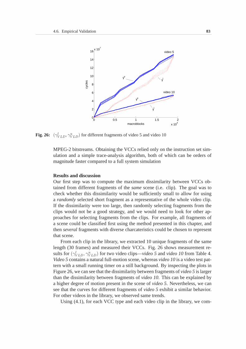
4.6. Empirical Validation 83
0 0.5 1 1.5 2
x 104
0
2
4
6
8
10
12
14
16x 10
7
macroblocks
cycl
es
γu
γl
γu
γl
video 5
video 5
video 10
Fig. 26: (γlV LD, γu
V LD) for different fragments of video 5 and video 10
MPEG-2 bitstreams. Obtaining the VCCs relied only on the instruction set sim-ulation and a simple trace-analysis algorithm, both of which can be orders ofmagnitude faster compared to a full system simulation
Results and discussionOur first step was to compute the maximum dissimilarity between VCCs ob-tained from different fragments of thesamescene (i.e. clip). The goal was tocheck whether this dissimilarity would be sufficiently small to allow for usinga randomlyselected short fragment as a representative of the whole video clip.If the dissimilarity were too large, then randomly selecting fragments from theclips would not be a good strategy, and we would need to look for other ap-proaches for selecting fragments from the clips. For example, all fragments ofa scene could be classified first using the method presented inthis chapter, andthenseveralfragments with diverse charcateristics could be chosen to representthat scene.
From each clip in the library, we extracted 10 unique fragments of the samelength (30 frames) and measured their VCCs. Fig. 26 shows measurement re-sults for(γl
V LD, γuV LD) for two video clips—video 5andvideo 10from Table 4.
Video 5contains a natural full-motion scene, whereasvideo 10is a video test pat-tern with a small running timer on a still background. By inspecting the plots inFigure 26, we can see that the dissimilarity between fragments ofvideo 5is largerthan the dissimilarity between fragments ofvideo 10. This can be explained bya higher degree of motion present in the scene ofvideo 5. Nevertheless, we cansee that the curves for different fragments ofvideo 5exhibit a similar behavior.For other videos in the library, we observed same trends.
Using (4.1), for each VCC type and each video clip in the library, we com-
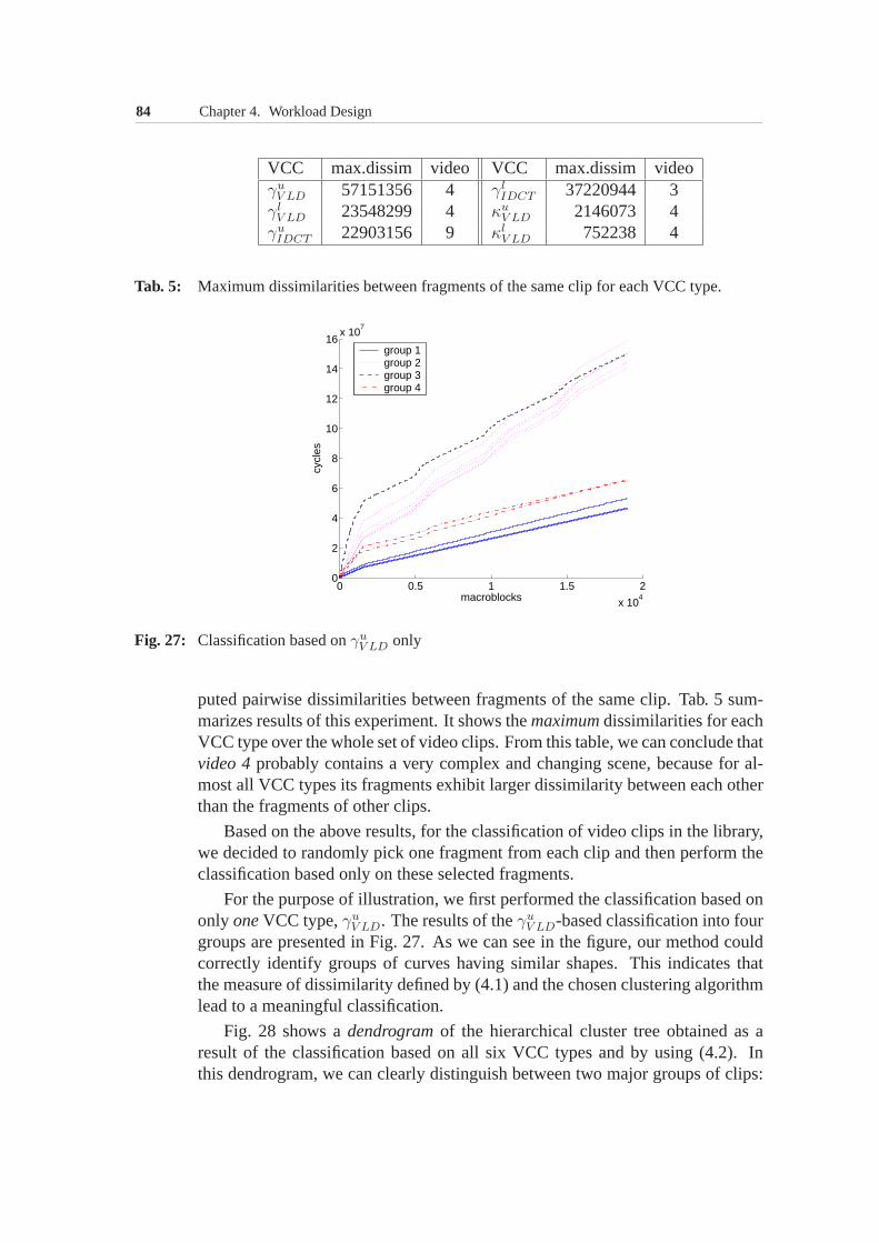
84 Chapter 4. Workload Design
VCC max.dissim video VCC max.dissim videoγu
V LD 57151356 4 γlIDCT 37220944 3
γlV LD 23548299 4 κu
V LD 2146073 4γu
IDCT 22903156 9 κlV LD 752238 4
Tab. 5: Maximum dissimilarities between fragments of the same clip for each VCC type.
0 0.5 1 1.5 2
x 104
0
2
4
6
8
10
12
14
16x 10
7
macroblocks
cycl
es
group 1group 2group 3group 4
Fig. 27: Classification based onγuV LD only
puted pairwise dissimilarities between fragments of the same clip. Tab. 5 sum-marizes results of this experiment. It shows themaximumdissimilarities for eachVCC type over the whole set of video clips. From this table, we can conclude thatvideo 4probably contains a very complex and changing scene, because for al-most all VCC types its fragments exhibit larger dissimilarity between each otherthan the fragments of other clips.
Based on the above results, for the classification of video clips in the library,we decided to randomly pick one fragment from each clip and then perform theclassification based only on these selected fragments.
For the purpose of illustration, we first performed the classification based ononly oneVCC type,γu
V LD. The results of theγuV LD-based classification into four
groups are presented in Fig. 27. As we can see in the figure, ourmethod couldcorrectly identify groups of curves having similar shapes.This indicates thatthe measure of dissimilarity defined by (4.1) and the chosen clustering algorithmlead to a meaningful classification.
Fig. 28 shows adendrogramof the hierarchical cluster tree obtained as aresult of the classification based on all six VCC types and by using (4.2). Inthis dendrogram, we can clearly distinguish between two major groups of clips:
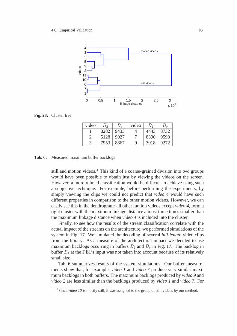
4.6. Empirical Validation 85
0 0.5 1 1.5 2 2.5 3
x 109
1 7 61011 2 9 5 3 8 4
linkage distance
vide
os
motion videos
still videos
Fig. 28: Cluster tree
video B2 Bv video B2 Bv
1 8282 9433 4 4443 87322 5128 9027 7 8390 95933 7953 8867 9 3018 9272
Tab. 6: Measured maximum buffer backlogs
still and motion videos.3 This kind of a coarse-grained division into two groupswould have been possible to obtain just by viewing the videoson the screen.However, a more refined classification would be difficult to achieve using sucha subjective technique. For example, before performing theexperiments, bysimply viewing the clips we could not predict thatvideo 4would have suchdifferent properties in comparison to the other motion videos. However, we caneasily see this in the dendrogram: all other motion videos exceptvideo 4, form atight cluster with the maximum linkage distance almost three times smaller thanthe maximum linkage distance whenvideo 4is included into the cluster.
Finally, to see how the results of the stream classification correlate with theactual impact of the streams on the architecture, we performed simulations of thesystem in Fig. 17. We simulated the decoding of severalfull-lengthvideo clipsfrom the library. As a measure of the architectural impact wedecided to usemaximum backlogs occurring in buffersB2 andBv in Fig. 17. The backlog inbufferB1 at thePE1’s input was not taken into account because of its relativelysmall size.
Tab. 6 summarizes results of the system simulations. Our buffer measure-ments show that, for example,video 1andvideo 7produce very similar maxi-mum backlogs in both buffers. The maximum backlogs producedby video 9andvideo 2are less similar than the backlogs produced byvideo 1andvideo 7. For
3Sincevideo 10is mostly still, it was assigned to the group of still videos by our method.
86 Chapter 4. Workload Design
video 9andvideo 2, the differences in the backlogs inB2 andBv are 2110 and245 macroblocks, respectively. We can also see thatvideo 9is more similar tovideo 2than tovideo 3. The maximum backlogs forvideo 3andvideo 9differin 4935 and 405 macroblocks forB2 andBv, respectively. Hence, we can con-clude that the simulation results exhibit the same tendencyas that shown by theclassification in Fig. 28.
4.7 SummaryIn this chapter, we presented an approach for workload design in the specificcontext of system-level performance evaluation of multimedia MpSoC architec-tures. The two main contributions of this chapter were: (i) establishing the utilityof VCCs as a model for multimedia workload characterization, and (ii) a work-load classification method based on VCCs which allows to identify groups ofmedia streams that impose similar workload on a platform architecture. Systemdesigners can use this classification method for constructing small representativeworkload sets for performance evaluation of MpSoC platforms for multimediaprocessing. We presented experimental results that validate and show usefulnessof this approach. However, there is a considerable scope forfurther research inthis direction. For example, a more systematic study needs to be done to identify“variability types” beyond the ones considered in this chapter.
5Designing Stream Scheduling Policies
In Chapter 4, we demonstrated one possible application of Variability Characteri-zation Curves: we proposed a method to automate the selectionof representativeworkload for performance evaluation of the multimedia MpSoC architectures.In this chapter, we demonstrate another application of VCCs. The focus of thischapter is on design ofplatform management policiesfor such MpSoC architec-tures.
A platform management policy specifies how the computational and commu-nication resources of an execution platform should be shared among applicationtasks, i.e. it defines the scheduling and arbitration1 policies implemented onthese resources. These policies are the knobs which designers can use to tune upthe system such that a desired tradeoff is achieved between system’s cost, perfor-mance and power consumption. That is why a proper selection and optimizationof platform management policies play an important role in the system-level de-sign of multimedia MpSoC platforms.
There is a large body of research work on real-time scheduling, coveringa broad spectrum of applications—from control-dominated to signal process-ing systems. However, the scheduling problems arising in the domain of me-dia processing execution platforms (such as multimedia MpSoC architectures)involve a number of specific issues that are not effectively addressed by the ex-isting scheduling methods: Due to the streaming nature of multimedia applica-tions, the scheduling of processing elements in a multimedia MpSoC architecturemore resembles scheduling of packet flows in a communicationnetwork than thetraditional real-time task scheduling. Many existing real-time task scheduling
1Hereafter, we use the termsschedulingandarbitration interchangeably.
88 Chapter 5. Designing Stream Scheduling Policies
techniques aredeadline-driven; in contrast, streaming multimedia applicationshavequality of service requirementswhich do not directly translate into taskdeadlines. Additionally, multimedia workloads are highlydynamic and variable,making it difficult to identify optimal scheduling strategies. As a result, platformmanagement policies for multimedia MpSoC architectures often have very largeand irregular design spaces.
All these factors call for new approaches to designing schedulers for mul-timedia MpSoC architectures. We explore this direction in this chapter. TheVCC-based workload model and the extended Modular Performance Analysisframework developed in Chapter 3 serve in this chapter as a basis for an efficientframework for design space exploration of the platform management policies. Inthis framework we mainly concentrate on fast and accurate performance evalua-tion methods and on schedulability tests which can effectively speedup and guidethe design space exploration process. To demonstrate the utility of the frame-work, we describe two case studies involving Time-DivisionMultiplex Access(TDMA) scheduling policy.
Contributions of this chapter
• We formulate the problem of scheduling media streams under strict QoS con-straints imposed by available buffer space. This problem ismotivated by thetight on-chip memory constraints associated with the current multimedia MpSoCarchitectures.
• We propose a framework for fast system-level design space exploration and op-timization of platform management policies for the media processing executionplatforms, such as multimedia MpSoC architectures. The framework features acombination of an initial one-time simulation of individual architectural compo-nents to obtain relevant workload characteristics, and a subsequent fastanalyticperformance evaluation, iteratively performed in the time-critical design spaceexploration loop.
• Based on the extended Modular Performance Analysis framework, we proposea method for computation of the buffer space requirements under different plat-form management policies. In comparison to the previously published methodsaddressing similar problems, the main novelty of our methodis in its ability toaccount for specific QoS requirements associated with processing media streamson buffer-constrained architectures. In addition, in thismethod we demonstratehow the VCC types defined in Section 3.3 can be used for themodular per-formance analysisof distributed heterogeneous architectures. By applying ourmethod to a case study of an MpSoC architecture, we demonstrate the complex-ity of the design space of the seemingly simple, widely used TDMA schedulingpolicy.
5.1. Stream Scheduling under Buffer Constraints 89
• We propose a method for a fast feasibility test ofstream schedulingpoliciesunder given QoS requirements. Towards this, we introduce the concept ofserviceboundsand show how they can be computed and used for the feasibilitytest.Through a detailed case study, we demonstrate how the service bounds can guidethe optimization of stream scheduling policies.
Organization of this chapter
• Section 5.1 introduces the problem of stream scheduling on buffer-constrainedarchitectures through a motivating example of aset-top boxapplication scenario.This scenario will be used in the course of this chapter for the case studies.
• Section 5.2 outlines the related work.
• Section 5.3 presents the framework for design space exploration and optimiza-tion of platform management policies for the media processing execution plat-forms.
• Section 5.4 addresses the problem of estimating buffer memory requirementsresulting from deploying different scheduling policies onprocessing elements ofan MpSoC architecture.
• Section 5.5 introduces the concept ofservice boundsused for quick feasibilitytests of stream schedulers for the buffer-constrained architectures.
• Section 5.6 concludes the chapter.
5.1 Stream Scheduling under Buffer ConstraintsThis section introduces the stream scheduling problem arising on the systemlevel in multimedia MpSoC architectures. We first describe aset-top boxappli-cation scenario; and then, using this scenario as an example, we introduce thescheduling problem and point out its specifics.
5.1.1 Set-top box application scenario
Fig. 29 shows a simple system-level model of a set-top box device implement-ing an audio-video decoder. Audio and video streams enter the device, whichincludes two PEs:PE1 andPE2. The MPEG-2 video decoding algorithm is par-titioned into two tasks—one mapped ontoPE1, the other ontoPE2. The MP3audio decoder includes a single task, mapped ontoPE2. On-chip buffersB1,B2,andB3 store the partially processed streams, whereasBv andBa, so calledplay-out buffers, store the fully decoded streams. These buffers are read by the video
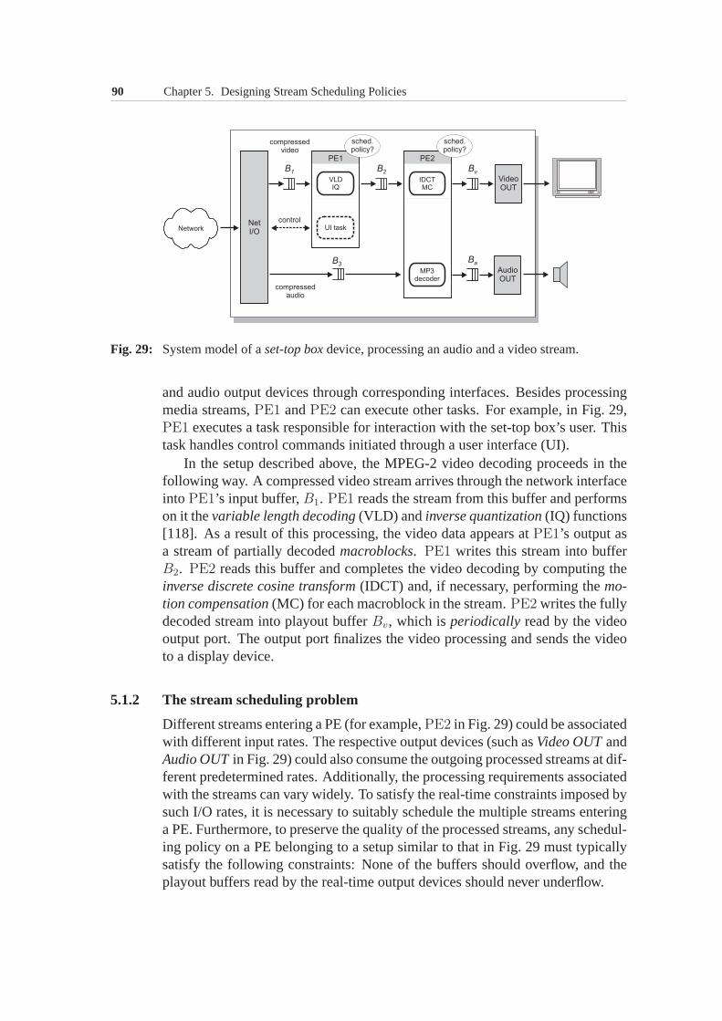
90 Chapter 5. Designing Stream Scheduling Policies
Fig. 29: System model of aset-top boxdevice, processing an audio and a video stream.
and audio output devices through corresponding interfaces. Besides processingmedia streams,PE1 andPE2 can execute other tasks. For example, in Fig. 29,PE1 executes a task responsible for interaction with the set-top box’s user. Thistask handles control commands initiated through a user interface (UI).
In the setup described above, the MPEG-2 video decoding proceeds in thefollowing way. A compressed video stream arrives through the network interfaceinto PE1’s input buffer,B1. PE1 reads the stream from this buffer and performson it thevariable length decoding(VLD) and inverse quantization(IQ) functions[118]. As a result of this processing, the video data appearsat PE1’s output asa stream of partially decodedmacroblocks. PE1 writes this stream into bufferB2. PE2 reads this buffer and completes the video decoding by computing theinverse discrete cosine transform(IDCT) and, if necessary, performing themo-tion compensation(MC) for each macroblock in the stream.PE2 writes the fullydecoded stream into playout bufferBv, which isperiodically read by the videooutput port. The output port finalizes the video processing and sends the videoto a display device.
5.1.2 The stream scheduling problem
Different streams entering a PE (for example,PE2 in Fig. 29) could be associatedwith different input rates. The respective output devices (such asVideo OUTandAudio OUTin Fig. 29) could also consume the outgoing processed streams at dif-ferent predetermined rates. Additionally, the processingrequirements associatedwith the streams can vary widely. To satisfy the real-time constraints imposed bysuch I/O rates, it is necessary to suitably schedule the multiple streams enteringa PE. Furthermore, to preserve the quality of the processed streams, any schedul-ing policy on a PE belonging to a setup similar to that in Fig. 29 must typicallysatisfy the following constraints: None of the buffers should overflow, and theplayout buffers read by the real-time output devices shouldnever underflow.
5.1. Stream Scheduling under Buffer Constraints 91
The output devices read the playout buffers at specified rates, depending onthe required output quality. Therefore, the constraint on such a buffers under-flow is to ensure that this required output quality is guaranteed. Guaranteeingthat none of the buffers overflows is needed because, in many cases, using block-ing writes to prevent the overflows is infeasible. Efficiently implementing suchblocking mechanisms requires either a multithreaded processor architecture orsubstantial run-time operating-system support for context switching, and neces-sitates platform-wide flow-control mechanisms [134, 151] which might be diffi-cult to implement in a distributed architecture.
The motivation for thisbuffer-centricdesign of schedulers is that buffers areavailable only at a very high premium because of their large on-chip area re-quirements [165]. On the other hand, the off-chip memory quickly becomes abottleneck in high bandwidth applications such as multimedia; and its bandwidthcannot be easily increased due to a number of technology constraints (e.g. a lim-ited number of I/O pins in a chip) [52]. Hence, the buffers play a central role inthe design of any scheduling or MpSoC platform management policy.
Specifics of the scheduling problemThe scheduling problem just described has a number of characteristics that makeit notably different from other real-time scheduling problems. These character-istics are summarized below.
• Implicit deadlines: The real-time scheduling traditionally relies on the notion of(hard and soft)deadlines: each task instance has anexplicit deadline. This way,the deadlines specify thereal-time constraintsto be satisfied by the scheduler.In contrast to this, in the stream scheduling problem the real-time constraints arenot naturally expressed through the deadlines. The main goal of a stream sched-uler is to satisfy theQoS requirementsassociated with the processed streams.Hence, the real-time constraints are determined by these QoS requirements. TheQoS requirements may, for example, include the required throughput, end-to-end processing delay2 and the underflow/overflow buffer constraints. In general,these QoS requirements do notdirectly translate into the deadlines.
In fact, the deadlines are not considered at all in the proposed method since weare not interested in individual task instances meeting their deadlines but in thewhole stream satisfying given QoS constraints. Although the deadlines are notspecified in the scheduling problem addressed in this chapter, thereal-time con-straintsstill exist and if needed can behard. Finally, we note that due to the highvariability of several workload characteristics and due tothe buffering involvedinto the stream processing, it would be difficult to translate the QoS requirementsinto the deadlines for each task instance without introducing a significant amountof pessimism and runtime overhead.
2The delay through the whole stream processing chain.
92 Chapter 5. Designing Stream Scheduling Policies
• “Too much service is as bad as too little service”:The goal of the conventionalreal-time scheduling is to improve task response times. Therefore, the moreservice a task gets, the better it is (provided that schedulability of other tasks isnot jeopardized). In contrast, in scheduling tasks processing streams under thebuffer constraints, providing too much service to a task maybe as dangerous asproviding too little service. A higher service rate offeredto a task increases theburstiness of the stream at the task’s output, and thereforemay cause overflows ofdownstream buffers. Hence, in stream scheduling we are seeking for abalancedservice.
• Asynchronous communication style:The majority of task models used in real-time scheduling assume that the tasks having data dependencies communicatesynchronously3: a next instance of a producer task is not allowed to start execu-tion before the output from the previous instance has been read by the consumertask. (The communication channel in this case represents a channel with de-structive write, i.e. aregister.) The underlying computation model of a streamprocessing application is different. In this model, tasks communicateasynchro-nouslythrough the buffered channels. This communication style relaxes the tim-ing coupling between dependent tasks, thereby creating a larger decision (or de-sign) space for a scheduler.
• Workload variability: As discussed in Section 3.1, there are not many taskmodels (and therefore scheduling techniques) that can effectively and efficientlyhandle the variable workloads. On the other hand, the major complication inscheduling of streaming multimedia applications on distributed execution plat-forms stems from the high workload variability, which leadsto bursty and com-plex communication traffic between the multimedia tasks.
The communication traffic on an MpSoC platform, such as the one shown inFig. 29, tends to be highly complex and bursty for three main reasons [165].First, the execution time of many media processing tasks highly depends on theproperties of the particular audio-video sample being processed [14, 57, 134].Second, the quantity of the I/O data consumed and produced bya task can alsovary widely. An example of this is the VLD task in Fig. 29. Third, the inputmedia streams already tend to be highly bursty when they enter a processingdevice. For example, in Fig. 29, the arrival pattern of the input streams enteringthe set-top box would depend on the networks congestion levels. In addition tothese effects, the burstiness in the streams arrival pattern could increase as theypass from one PE to the next, depending on these PEs’ congestion levels andscheduling policies [133].
3See the discussion in Section 3.1.
5.2. Related work 93
5.2 Related workIn real-time scheduling, the QoS requirements of tasks are typically specifiedwith deadlines (which are explicit and fixed for a given task). Thus, many exist-ing scheduling methods proposed in this area are “deadline-driven” [41, 150].4
However, there is a class of real-time tasks which rather require a guaranteedrate of progress(average throughput) than the satisfaction of the fixed deadlines[140]. Tasks that process continuous media streams fall into this category. Thereare scheduling techniques that can guarantee the required average throughput tosuch tasks in presence of other tasks by effectivelyreservinga portion of theprocessor bandwidth for execution of these tasks. Examplesof such techniquesinclude various kinds of aperiodic taskservers[1, 22, 94, 147, 152] and therate-based executionmodel [65]. Scheduling techniques based on the bandwidthreservation principle are also used to guarantee QoS to packet flows in commu-nication networks (see e.g. [179]). The same principle can also be applied toschedule streams on an MpSoC execution platform. The scheduling techniquesmentioned above may serve as a basis for designing platform management poli-cies for the media processors. However, their direct application in this domain islimited because most of them are concerned with scheduling of a single PE (e.g.a processor or a communication link) without considering system-level issuessuch as the restricted buffer space.
There is a large body of research on scheduling of directed acyclic task graphson multiprocessor architectures [40, 76, 80]. A task graph specifies precedencerelations between tasks. These relations model data dependencies between thetasks. An application is typically modeled by asetof independent task graphs;each task graph is associated with a deadline and an activation period. Thisset is then scheduled on heterogeneous architectures [98, 132]. Several hard-ware/software co-synthesis frameworks use this model [32,33, 35]. The methodin [32] schedules task graphs with periodic and aperiodic activations. To guar-antee QoS to aperiodic task graphs it employs resource reservations. [127] pro-poses an algorithm to schedule task graphs which model both data and controldependencies. Only a few approaches in this category consider memory con-straints while scheduling the tasks [108, 131, 154].
All scheduling methods just mentioned assumesingle-rate data dependen-ciesbetween tasks, i.e. the execution rate of any consumer task exactly matchesthe execution rate of the corresponding producer task. Thistask model is toorestrictive for a large class of multimedia applications inwhich tasks havemulti-rate data dependencies[67]. A more adequate task model for multimedia appli-cations relies on the concept of dataflow process networks [89], which permitsthe multi-rate data dependencies as well as cycles in the task graph. Schedulingof dataflow process networks on multiprocessor architectures received a lot ofattention in the digital signal processing (DSP) domain [50, 88, 149]. The basic
4Some of these methods have been mentioned in Section 3.1.
94 Chapter 5. Designing Stream Scheduling Policies
model used to represent DSP applications, called Synchronous Dataflow (SDF),assumes tasks with constant I/O rates [88]. A generalization of this model, thecyclo-static dataflow[19], allows for the I/O rates to cyclically change. Schedul-ing of the dataflow graphs is mainly concerned with minimization of data andprogram memory needed to execute a graph [18]. Although different tasks mayexecute at different rates, all these rates are tightly related to each other and fixed.
The existing dataflow scheduling algorithms focus on scheduling of only onegraph, ignoring the fact that several independent graphs, each having its own QoSrequirements, may need to be concurrently executed on the target architecture.Combining these algorithms with the results known from real-time scheduling(e.g. with the bandwidth reservation techniques discussedabove) may help toaddress this problem. An interesting approach going in thisdirection is presentedin [43] where the rate-based execution model [65] based onearliest deadline firstpolicy is used to schedule an SDF graph on a single processor architecture. Forthis setup, [65] provides an analysis of buffer requirements and the latency.
A number ofsystem-level performance analysisframeworks have been pro-posed in the literature for evaluation and optimization of platform managementpolicies. [71] proposes a framework for evaluation of run-time schedulers inembedded multimedia systems. Given a system architecture,a set of periodictask graphs with execution times characterized by probability distributions, anda scheduling policy implemented on PEs of the architecture,for each task graphthe framework in [71] computes a probability distribution of the processing de-lay. The framework in [129] performs a system-level schedulability analysis ofdistributed real-time systems which rely on the time-triggered protocol (TTP)[76] as the communication infrastructure. Along with the schedulability tests,[129] reports techniques to optimize the parameters of the TTP-based commu-nication infrastructure and select suitable message passing strategies for it. Thework in [51] uses evolutionary multi-objective optimization techniques and theSymTA/S performance evaluation framework [68, 133] to find suitable periodand time slot lengths of the TDMA scheduling policy. [25, 156] address theproblem of performance evaluation and design space exploration of networkprocessors. Similar to the framework presented in this chapter, the approachin [25, 156] relies on the Real-Time Calculus [121, 158]. It estimates variousperformance metrics, such as required buffer sizes and packet delays, resultingfrom implementing different scheduling policies on PEs of anetwork processor.However, unlike the framework presented in this chapter, the work in [25, 156]does not account for the buffer constraints (especially those related to theplay-out buffers) and the variability of the task I/O rates, which are naturalfor me-dia stream processing on distributed execution platforms,such as multimediaMpSoC architectures.
Finally, we note that designing schedulers for on-chip PEs involves signif-icantly different constraints from those for scheduling and buffer managementof multimedia applications in operating systems and communication networks
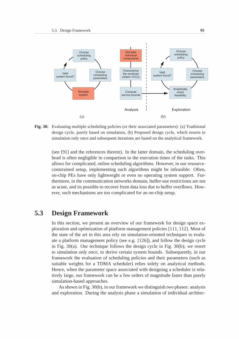
5.3. Design Framework 95
(a) (b)
Fig. 30: Evaluating multiple scheduling policies (or their associated parameters): (a) Traditionaldesign cycle, purely based on simulation, (b) Proposed design cycle, which resorts tosimulation only once and subsequent iterations are based on the analytical framework.
(see [91] and the references therein). In the latter domain,the scheduling over-head is often negligible in comparison to the execution times of the tasks. Thisallows for complicated, online scheduling algorithms. However, in our resource-constrained setup, implementing such algorithms might be infeasible: Often,on-chip PEs have only lightweight or even no operating system support. Fur-thermore, in the communication networks domain, buffer-use restrictions are notas acute, and its possible to recover from data loss due to buffer overflows. How-ever, such mechanisms are too complicated for an on-chip setup.
5.3 Design FrameworkIn this section, we present an overview of our framework for design space ex-ploration and optimization of platform management policies [111, 112]. Most ofthe state of the art in this area rely on simulation-orientedtechniques to evalu-ate a platform management policy (see e.g. [126]), and follow the design cyclein Fig. 30(a). Our technique follows the design cycle in Fig.30(b); we resortto simulationonly once, to derive certain system bounds. Subsequently, in ourframework the evaluation of scheduling policies and their parameters (such assuitable weights for a TDMA scheduler) relies solely on analytical methods.Hence, when the parameter space associated with designing ascheduler is rela-tively large, our framework can be a few orders of magnitude faster than purelysimulation-based approaches.
As shown in Fig. 30(b), in our framework we distinguish two phases: analysisand exploration. During the analysis phase a simulation of individual architec-
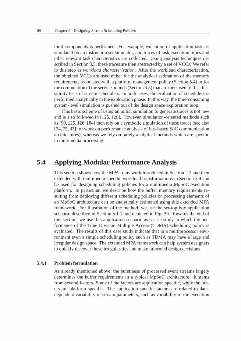
96 Chapter 5. Designing Stream Scheduling Policies
tural components is performed. For example, execution of application tasks issimulated on an instruction set simulator, and traces of task execution times andother relevant task characteristics are collected. Using analysis techniques de-scribed in Section 3.5, these traces are then abstracted by aset of VCCs. We referto this step asworkload characterization. After the workload characterization,the obtained VCCs are used either for the analytical estimation of the memoryrequirements associated with a platform management policy(Section 5.4) or forthe computation of the service bounds (Section 5.5) that arethen used for fast fea-sibility tests of stream schedulers. In both cases, the evaluation of schedulers isperformed analytically in the exploration phase. In this way, the time-consumingsystem-level simulation is pushed out of the design space exploration loop.
This basic scheme of using an initial simulation to generatetraces is not newand is also followed in [125, 126]. However, simulation-oriented methods suchas [99, 125, 126, 184] then rely on a symbolic simulation of these traces (see also[74, 75, 83] for work on performance analysis of bus-based SoC communicationarchitectures), whereas we rely on purely analytical methods which are specificto multimedia processing.
5.4 Applying Modular Performance AnalysisThis section shows how the MPA framework introduced in Section 2.2 and thenextended with multimedia-specific workload transformations in Section 3.4 canbe used for designing scheduling policies for a multimedia MpSoC executionplatform. In particular, we describe how the buffer memory requirements re-sulting from deploying different scheduling policies on processing elements ofan MpSoC architecture can be analytically estimated using this extended MPAframework. For illustration of the method, we use the set-top box applicationscenario described in Section 5.1.1 and depicted in Fig. 29.Towards the end ofthis section, we use this application scenario as a case study in which the per-formance of the Time Division Multiple Access (TDMA) scheduling policy isevaluated. The results of this case study indicate that in a multiprocessor envi-ronment even a simple scheduling policy such as TDMA may havea large andirregular design space. The extended MPA framework can helpsystem designersto quickly discover these irregularities and make informeddesign decisions.
5.4.1 Problem formulation
As already mentioned above, the burstiness of processed event streams largelydetermines the buffer requirements in a typical MpSoC architecture. It stemsfrom several factors. Some of the factors are application specific, while the oth-ers are platform specific. The application specific factors are related to data-dependent variability of stream parameters, such as variability of the execution
5.4. Applying Modular Performance Analysis 97
Fig. 31: A chain of performance components induced in a scheduling network by a media stream.
demand. The burstiness caused by the platform specific factors is associatedwith contention of event streams on shared communication and computationalresources (PEs) of the architecture. The scheduling and arbitration policies usedto manage the access to these resources influence the degree of the burstiness in-duced in the event streams and, therefore, largely determine the amount of bufferspace required to process these streams at a certain QoS level.
Scheduling policies can be designed such that the buffer space requirementsare minimized. However, in many cases, besides the minimization of the bufferspace, there are also other design criteria. These criteriaare often in conflictwith the buffer space minimization goal. For example, minimizing the bufferrequirements necessitates scheduling streams at a finer granularity. However,this may increase scheduling overhead and, therefore, result in wasting precioussystem resources (e.g. energy). While designing schedulingstrategies for mediaprocessors, system designers are often concerned with identifying such trade-offs. In many cases, these tradeoffs are difficult to identify since they representcomplex relationships between the application at hand and different system pa-rameters, including those pertaining to the resource sharing policies. Identifyingthese tradeoffs, therefore, necessitates evaluation of many alternative points inthe design space. One of the major problems in this context ishow to quicklyevaluate a large number of the design points. The method proposed in this sec-tion employs the MPA framework to address this problem.
In order to use the MPA framework, we need to formulate our problem as ascheduling network. Such a scheduling network represents a performance modelof a given application-to-architecture mapping. It specifies how event streamsflow between different PEs of the architecture and how these PEs are shared be-tween those streams. The scheduling network, therefore, consists of performancecomponents interconnected through resource and event flows(see Section 2.2 fordetails). Concrete instances of event and resource flows are abstracted by arrivaland service curves,α = (αl, αu) andβ = (βl, βu). Additionally, in the MPAframework with multimedia extensions, performance components are character-ized by consumption, production and execution demand curves, i.e. each com-ponent is associated with VCCsκ = (κl, κu), π = (πl, πu), andγ = (γl, γu).
Consider a chain of performance componentsC1 → C2 → . . . → Ci →
98 Chapter 5. Designing Stream Scheduling Policies
. . . → Cn−1 → Cn induced in a scheduling network by a media stream, asshown in Fig. 31. This chain models a sequence of tasks mappedonto differentPEs of the architecture, which process the media stream in a pipelined fashion.In Fig. 31, performance componentCi (i = 1, 2, . . .) has as its input event-basedarrival curveαi. This curve is transformed byCi into event-based arrival curveαi+1. αi+1, appearing atCi’s output, serves as an input to the next performancecomponent in the chain,Ci+1. The way in whichCi transformsαi into αi+1
depends on the workload variability atCi, specified by VCCs(κi, πi, γi), and onthe scheduling policy implemented on the PE with whichCi is associated. Thescheduling policy determines the amount of resources (e.g.processor cycles)received byCi from the PE in any given time interval. This amount is modeledby resource-based service curveβi. In other words,βi characterizes the serviceoffered to the media stream on the PE.
At the input of each performance component, there is an implicit buffer (notshown in Fig. 31). As explained above, to maintain the quality of the processedmedia stream at an acceptable level, we require that none of the buffers in theprocessing chain ever overflows. Furthermore, there may be some performancecomponents in the processing chain whose input has to be continuous. Thismeans that they cannot tolerate waiting on the empty input buffer for new eventsto arrive. Whenever such a component reads from the buffer, the data mustbe available for it. We refer to such buffers asplayout buffers. Typically, aplayout buffer is associated with the last performance component in a processingchain. This is because the last component often represents an output interface ina multimedia MpSoC architecture, e.g. a video or audio output, at which eventstreams have to satisfy strict real-time constraints imposed by external devices(such as digital-to-analog converters). Again, to ensure an acceptable quality ofthe processed stream, we require that any playout buffer neither overflows norunderflows.
Assume that, in Fig. 31,Cn represents the performance component that needsto have at its input a playout buffer. To model the timing withwhichCn reads itsplayout buffer, we useevent-basedservice curvesβl
n andβun. βl
n(∆) andβun(∆)
specify, respectively, the minimum and the maximum number of events (streamobjects) thatCn reads from the playout buffer within any time interval of length∆.
Given a processing chain such as one shown in Fig. 31, our goalis to computethe maximal backlog which may occur in each of the buffers in this processingchain as a result of applying a given scheduling policy. After finding the maximalbacklog in each of the buffers, we will be able to compute the maximum memoryrequirements associated with this scheduling policy.
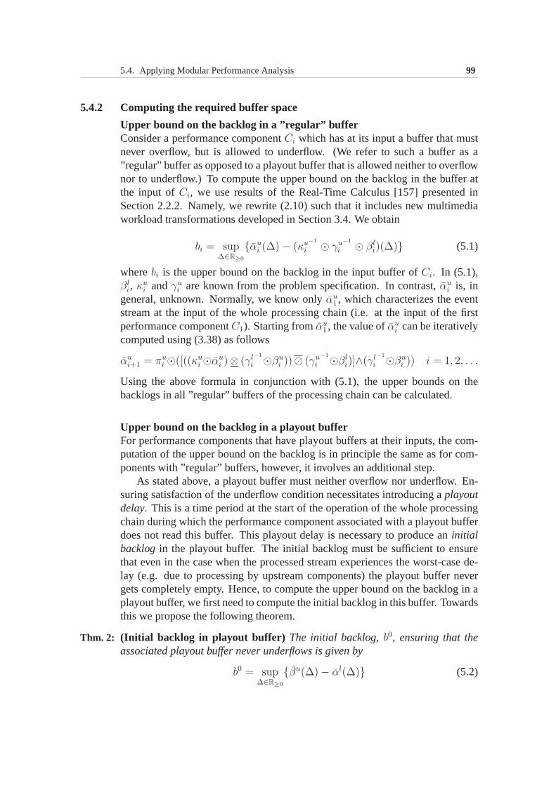
5.4. Applying Modular Performance Analysis 99
5.4.2 Computing the required buffer space
Upper bound on the backlog in a ”regular” bufferConsider a performance componentCi which has at its input a buffer that mustnever overflow, but is allowed to underflow. (We refer to such abuffer as a”regular” buffer as opposed to a playout buffer that is allowed neither to overflownor to underflow.) To compute the upper bound on the backlog inthe buffer atthe input ofCi, we use results of the Real-Time Calculus [157] presented inSection 2.2.2. Namely, we rewrite (2.10) such that it includes new multimediaworkload transformations developed in Section 3.4. We obtain
bi = sup∆∈R≥0
{αui (∆) − (κu−1
i ⊙ γu−1
i ⊙ βli)(∆)} (5.1)
wherebi is the upper bound on the backlog in the input buffer ofCi. In (5.1),βl
i, κui andγu
i are known from the problem specification. In contrast,αui is, in
general, unknown. Normally, we know onlyαu1 , which characterizes the event
stream at the input of the whole processing chain (i.e. at theinput of the firstperformance componentC1). Starting fromαu
1 , the value ofαui can be iteratively
computed using (3.38) as follows
αui+1 = πu
i ⊙([((κui ⊙αu
i )⊗ (γl−1
i ⊙βui ))⊘ (γu−1
i ⊙βli)]∧(γl−1
i ⊙βui )) i = 1, 2, . . .
Using the above formula in conjunction with (5.1), the upperbounds on thebacklogs in all ”regular” buffers of the processing chain can be calculated.
Upper bound on the backlog in a playout bufferFor performance components that have playout buffers at their inputs, the com-putation of the upper bound on the backlog is in principle thesame as for com-ponents with ”regular” buffers, however, it involves an additional step.
As stated above, a playout buffer must neither overflow nor underflow. En-suring satisfaction of the underflow condition necessitates introducing aplayoutdelay. This is a time period at the start of the operation of the whole processingchain during which the performance component associated with a playout bufferdoes not read this buffer. This playout delay is necessary toproduce aninitialbacklogin the playout buffer. The initial backlog must be sufficientto ensurethat even in the case when the processed stream experiences the worst-case de-lay (e.g. due to processing by upstream components) the playout buffer nevergets completely empty. Hence, to compute the upper bound on the backlog in aplayout buffer, we first need to compute the initial backlog in this buffer. Towardsthis we propose the following theorem.
Thm. 2: (Initial backlog in playout buffer) The initial backlog,b0, ensuring that theassociated playout buffer never underflows is given by
b0 = sup∆∈R≥0
{βu(∆) − αl(∆)} (5.2)
100 Chapter 5. Designing Stream Scheduling Policies
whereαl denotes the lower event-based arrival curve of the stream at the inputof the playout buffer, andβu denotes the upper event-based service curve offeredto the stream by the performance component reading the playout buffer.
Proof. Letx(t) denote the total number of events that have arrived in the playoutbuffer within time interval[0, t]. Similarly, let y(t) denote the total number ofevents that have been read out of the playout buffer within time interval[0, t].Assume thatx(0) = y(0) = 0. From the definitions of the arrival and servicecurves, we havex(t + s) − x(t) ≥ αl(s) andy(t + s) − y(t) ≤ βu(s) for alls, t ∈ R≥0 [85]. The playout buffer never underflows ifx(t) > y(t) for allt ∈ R>0.
Now, consider somet up to which the conditionx(t) > y(t) holds. To ensurethat this condition also holds for somet′ = t+ s the following relation has to besatisfied
x(t) + αl(s) ≥ y(t) + βu(s) ∀t, s ∈ R>0
Here, αl (s) is the minimum number of events that may arrive in the interval[t, t + s], whereasβu (s) is the maximum number of events that can be read outof the playout buffer in the same interval. Letb(t) = x(t) − y(t) denote thebacklog in the buffer at timet. Then we have
b(t) ≥ βu(s) − αl(s) ∀t, s ∈ R>0
By putting t = 0 in the above condition, we obtain a constraint for the initialbacklogb(0) ≥ βu(s) − αl(s) for all s ∈ R>0. This is equivalent to requiringthatb(0) ≥ b0, whereb0 = sups∈R≥0
{βu(s) − αl(s)}�
Whenever even-based service curveβui is specified, we can directly use (5.2)
to compute initial backlogb0i in the playout buffer ofCi. Otherwise, we need toapply corresponding workload transformations to resource-based service curveβu
i . After applying these transformations, (5.2) takes the following form.
b0i = sup∆∈R≥0
{(κl−1
i ⊙ γl−1
i ⊙ βui )(∆) − αl
i(∆)} (5.3)
In (5.3), αli can be computed in a similar way asαu
i , as explained above, butusing (3.39):
αli+1 = πl
i ⊙ ([(κli ⊙ αl
i ⊘ γl−1
i ⊙ βui )⊗ γu−1
i ⊙ βli] ∧ γu−1
i ⊙ βli)
The computation of the above formula starts fromαl1 (which is known from the
problem specification) and iteratively proceeds up to the required indexi.Taking into account the required initial backlogb0i , the upper bound on the
backlog in the playout buffer at the input of the performancecomponentCi canbe calculated as
b∗i = b0i + bi (5.4)
wherebi is determined by (5.1).
5.4. Applying Modular Performance Analysis 101
Maximum memory requirementsHaving computed the upper bounds on the backlogs in the buffers within a streamprocessing chain, we can calculate the maximum memory requirement associ-ated with this chain. For this, letSi denote the maximum size of a stream objectin the input buffer of performance componentCi. Then the maximum memoryrequirement,M, of the whole processing chain can be computed as follows.
M =n
∑
i=1
bi × Si +∑
∀i∈P
b0i × Si (5.5)
whereP = {i : Ci has at its input a playout buffer}.
5.4.3 Illustrative case study
This subsection presents results of a case study published in [115], where theconcepts of the modular performance analysis and the new VCC types developedin the previous sections of the thesis are applied to evaluate performance of theTDMA scheduling policy in a multiprocessor environment. This multiproces-sor environment is represented by the system architecture shown in Fig. 29. Inthis architecture, the TDMA scheduling policy is used for scheduling processingelementsPE1 andPE2, with each PE having its own TDMA scheduler.
There are three main reasons for choosing TDMA for this case study. First,it is simple enough to implement in a SoC setup, and it has low scheduling over-head, therefore it is widely used for scheduling on-chip PEsand communicationresources [44, 76, 129]. Second, since TDMA is fully predictable in terms of theworst-case delay and bandwidth provided to individual event flows, it is espe-cially suitable for scheduling media streaming applications associated with real-time guarantees. Third, TDMA is also relatively easy to characterize in terms ofservice curves; hence, it provides a simple illustration ofthe theoretical conceptspresented above. However, it may be noted here that our evaluation frameworkis not restricted to analyzing only TDMA schedulers. Systemdesigners can useit to analyze any static- or dynamic-priority scheduling algorithm, including pre-emptive and nonpreemptive versions. These include scheduling policies suchas fixed-priority, weighted round-robin, and earliest-deadline first. In fact, ourframework can evaluate any scheduling policy that is characterizable using ser-vice curves. Moreover, it can evaluate a platform in which different schedulingpolicies are used on the different PEs [24].
For this case study, we consider the set-top box applicationscenario de-scribed in Section 5.1.1 and also shown in Fig. 29. In this scenario, each PEprocesses two independent concurrent event flows.PE1 performs partial decod-ing of the MPEG-2 video stream (by applying to it VLD and IQ functions) andhandles control events (e.g. user’s commands).PE2 finalizes the decoding ofthe MPEG-2 stream (with IDCT and MC functions) and decodes an MP3 audiostream. The TDMA schedulers, therefore, regulate sharing of PE1 andPE2 by
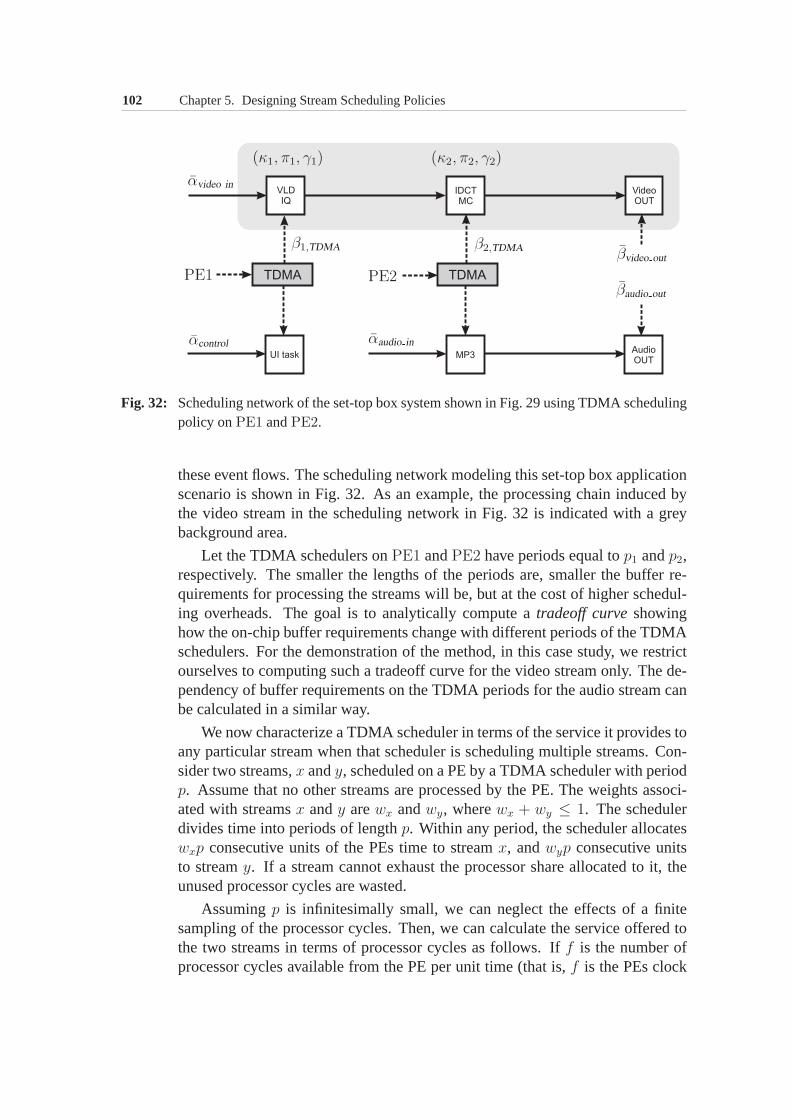
102 Chapter 5. Designing Stream Scheduling Policies
Fig. 32: Scheduling network of the set-top box system shown in Fig. 29 using TDMA schedulingpolicy onPE1 andPE2.
these event flows. The scheduling network modeling this set-top box applicationscenario is shown in Fig. 32. As an example, the processing chain induced bythe video stream in the scheduling network in Fig. 32 is indicated with a greybackground area.
Let the TDMA schedulers onPE1 andPE2 have periods equal top1 andp2,respectively. The smaller the lengths of the periods are, smaller the buffer re-quirements for processing the streams will be, but at the cost of higher schedul-ing overheads. The goal is to analytically compute atradeoff curveshowinghow the on-chip buffer requirements change with different periods of the TDMAschedulers. For the demonstration of the method, in this case study, we restrictourselves to computing such a tradeoff curve for the video stream only. The de-pendency of buffer requirements on the TDMA periods for the audio stream canbe calculated in a similar way.
We now characterize a TDMA scheduler in terms of the service it provides toany particular stream when that scheduler is scheduling multiple streams. Con-sider two streams,x andy, scheduled on a PE by a TDMA scheduler with periodp. Assume that no other streams are processed by the PE. The weights associ-ated with streamsx andy arewx andwy, wherewx + wy ≤ 1. The schedulerdivides time into periods of lengthp. Within any period, the scheduler allocateswxp consecutive units of the PEs time to streamx, andwyp consecutive unitsto streamy. If a stream cannot exhaust the processor share allocated toit, theunused processor cycles are wasted.
Assumingp is infinitesimally small, we can neglect the effects of a finitesampling of the processor cycles. Then, we can calculate theservice offered tothe two streams in terms of processor cycles as follows. Iff is the number ofprocessor cycles available from the PE per unit time (that is, f is the PEs clock
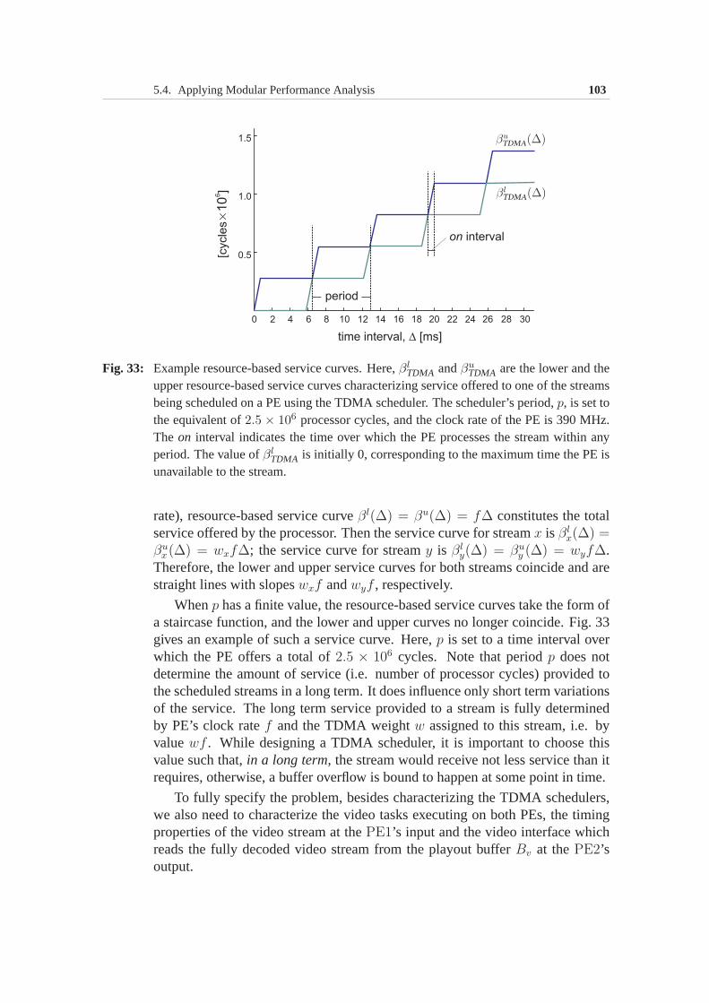
5.4. Applying Modular Performance Analysis 103
Fig. 33: Example resource-based service curves. Here,βlTDMA andβu
TDMA are the lower and theupper resource-based service curves characterizing service offered to one of the streamsbeing scheduled on a PE using the TDMA scheduler. The scheduler’s period, p, is set tothe equivalent of2.5 × 106 processor cycles, and the clock rate of the PE is 390 MHz.The on interval indicates the time over which the PE processes the stream within anyperiod. The value ofβl
TDMA is initially 0, corresponding to the maximum time the PE isunavailable to the stream.
rate), resource-based service curveβl(∆) = βu(∆) = f∆ constitutes the totalservice offered by the processor. Then the service curve forstreamx is βl
x(∆) =βu
x(∆) = wxf∆; the service curve for streamy is βly(∆) = βu
y (∆) = wyf∆.Therefore, the lower and upper service curves for both streams coincide and arestraight lines with slopeswxf andwyf , respectively.
Whenp has a finite value, the resource-based service curves take the form ofa staircase function, and the lower and upper curves no longer coincide. Fig. 33gives an example of such a service curve. Here,p is set to a time interval overwhich the PE offers a total of2.5 × 106 cycles. Note that periodp does notdetermine the amount of service (i.e. number of processor cycles) provided tothe scheduled streams in a long term. It does influence only short term variationsof the service. The long term service provided to a stream is fully determinedby PE’s clock ratef and the TDMA weightw assigned to this stream, i.e. byvaluewf . While designing a TDMA scheduler, it is important to choose thisvalue such that,in a long term, the stream would receive not less service than itrequires, otherwise, a buffer overflow is bound to happen at some point in time.
To fully specify the problem, besides characterizing the TDMA schedulers,we also need to characterize the video tasks executing on both PEs, the timingproperties of the video stream at thePE1’s input and the video interface whichreads the fully decoded video stream from the playout bufferBv at thePE2’soutput.
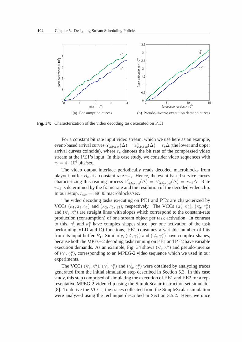
104 Chapter 5. Designing Stream Scheduling Policies
(a) Consumption curves (b) Pseudo-inverse execution demand curves
Fig. 34: Characterization of the video decoding task executed onPE1.
For a constant bit rate input video stream, which we use here as an example,event-based arrival curvesαl
video in(∆) = αuvideo in(∆) = rc∆ (the lower and upper
arrival curves coincide), whererc denotes the bit rate of the compressed videostream at thePE1’s input. In this case study, we consider video sequences withrc = 4 · 106 bits/sec.
The video output interface periodically reads decoded macroblocks fromplayout bufferBv at a constant ratermb. Hence, the event-based service curvescharacterizing this reading processβl
video out(∆) = βuvideo out(∆) = rmb∆. Rate
rmb is determined by the frame rate and the resolution of the decoded video clip.In our setup,rmb = 39600 macroblocks/sec.
The video decoding tasks executing onPE1 andPE2 are characterized byVCCs (κ1, π1, γ1) and (κ2, π2, γ2), respectively. The VCCs(πl
1, πu1 ), (πl
2, πu2 )
and(κl1, κ
u1) are straight lines with slopes which correspond to the constant-rate
production (consumption) of one stream object per task activation. In contrastto this, κl
1 andκu1 have complex shapes since, per one activation of the task
performing VLD and IQ functions,PE1 consumes a variable number of bitsfrom its input bufferB1. Similarly, (γl
1, γu1 ) and(γl
2, γu2 ) have complex shapes,
because both the MPEG-2 decoding tasks running onPE1 andPE2 have variableexecution demands. As an example, Fig. 34 shows(κl
1, κu1) and pseudo-inverse
of (γl1, γ
u1 ), corresponding to an MPEG-2 video sequence which we used in our
experiments.
The VCCs(κl1, κ
u1), (γl
1, γu1 ) and(γl
2, γu2 ) were obtained by analyzing traces
generated from the initial simulation step described in Section 5.3. In this casestudy, this step comprised of simulating the execution ofPE1 andPE2 for a rep-resentative MPEG-2 video clip using the SimpleScalar instruction set simulator[8]. To derive the VCCs, the traces collected from the SimpleScalar simulationwere analyzed using the technique described in Section 3.5.2. Here, we once
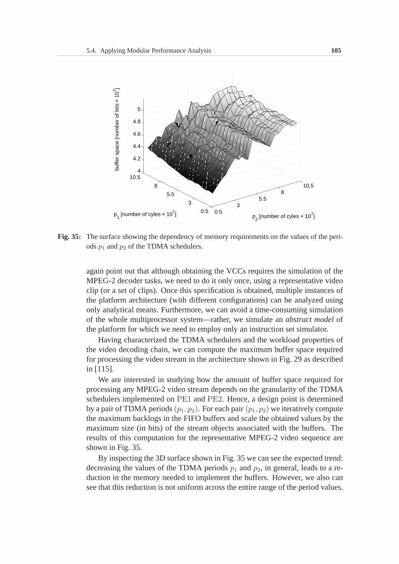
5.4. Applying Modular Performance Analysis 105
0.53
5.58
10.5
0.5
3
5.5
8
10.54
4.2
4.4
4.6
4.8
5
p2 [number of cyles × 107]p
1 [number of cyles × 107]
buffe
r sp
ace
[num
ber
of b
its ×
107 ]
Fig. 35: The surface showing the dependency of memory requirements on the values of the peri-odsp1 andp2 of the TDMA schedulers.
again point out that although obtaining the VCCs requires the simulation of theMPEG-2 decoder tasks, we need to do it only once, using a representative videoclip (or a set of clips). Once this specification is obtained,multiple instances ofthe platform architecture (with different configurations)can be analyzed usingonly analytical means. Furthermore, we can avoid a time-consuming simulationof the whole multiprocessor system—rather, we simulate anabstract modelofthe platform for which we need to employ only an instruction set simulator.
Having characterized the TDMA schedulers and the workload properties ofthe video decoding chain, we can compute the maximum buffer space requiredfor processing the video stream in the architecture shown inFig. 29 as describedin [115].
We are interested in studying how the amount of buffer space required forprocessing any MPEG-2 video stream depends on the granularity of the TDMAschedulers implemented onPE1 andPE2. Hence, a design point is determinedby a pair of TDMA periods(p1, p2). For each pair(p1, p2) we iteratively computethe maximum backlogs in the FIFO buffers and scale the obtained values by themaximum size (in bits) of the stream objects associated withthe buffers. Theresults of this computation for the representative MPEG-2 video sequence areshown in Fig. 35.
By inspecting the 3D surface shown in Fig. 35 we can see the expected trend:decreasing the values of the TDMA periodsp1 andp2, in general, leads to a re-duction in the memory needed to implement the buffers. However, we also cansee that this reduction is not uniform across the entire range of the period values.
106 Chapter 5. Designing Stream Scheduling Policies
Even for a simple scheduling discipline like TDMA, there arelarge irregulari-ties in the design space. This makes it virtually impossibleto come up with anappropriate tradeoff, based only on a designer’s experience on how the mem-ory requirements typically change with small changes in theparameters of theschedulers. Since on-chip buffers have large area requirements, such an infor-mation about the design space is, however, essential for determining optimalplatform management policies. Using our framework it is therefore possible todiscover the irregularities in the design space, and from itarrive at an appropri-ate tradeoff—in this case between scheduling overheads andbuffer requirements.This capability of the framework can be attributed to the underlying concept ofVCCs which can be used to precisely represent the different types of variabilitiesassociated with multimedia processing on multiprocessor SoC platforms.
Finally, we note that evaluating a single design point(p1, p2) by simulatingan abstract transaction-level model of the platform architecture in SystemC [153](using the system simulator described in Appendix A) for a2 sec long video cliprequired almost an hour of simulation time. This simulationtime was around100 times longer than the time needed for evaluating a designpoint with ouranalytical framework implemented using a combination of Mathematica5 andMatlab6 models. (We believe that an efficient C/C++ implementation would beat least 5-10 times faster than our current prototype implementation of the an-alytical framework.) Considering the time involved in simulating even a singledesign point for a relatively short video clip, it is almost infeasible to obtain adesign surfacesuch as the one shown in Fig. 35 in a reasonable time using purelysimulation-based techniques. In contrast, using the proposed analytical frame-work system designers can learn about the structure of the entire design space intens of minutes.
5.5 Checking Feasibility of Stream Schedulers
In this section, we introduce the concept ofservice bounds[102, 103, 111]. Theservice bounds allow to quickly verify whether in principlethere exists a schedul-ing policy that can satisfy QoS requirements of a stream (such as the delay andbuffer constraints), and to check feasibility of a given scheduler against theserequirements. Furthermore, they can direct the design space exploration processby providing the information by how much a given scheduler does not (or does)satisfy a given set of QoS requirements.
In this section, we limit the presentation to the service bounds obtained fromthe buffer constraints; however, the principles presentedin this section can beapplied to derive the service bounds also for the delay constraints.
5http://www.wolfram.com6http://www.mathworks.com
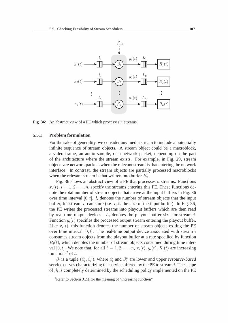
5.5. Checking Feasibility of Stream Schedulers 107
Fig. 36: An abstract view of a PE which processesn streams.
5.5.1 Problem formulation
For the sake of generality, we consider any media stream to include a potentiallyinfinite sequence of stream objects. A stream object could bea macroblock,a video frame, an audio sample, or a network packet, depending on the partof the architecture where the stream exists. For example, inFig. 29, streamobjects are network packets when the relevant stream is thatentering the networkinterface. In contrast, the stream objects are partially processed macroblockswhen the relevant stream is that written into bufferB2.
Fig. 36 shows an abstract view of a PE that processesn streams. Functionsxi(t), i = 1, 2, . . . , n, specify the streams entering this PE. These functions de-note the total number of stream objects that arrive at the input buffers in Fig. 36over time interval[0, t]. li denotes the number of stream objects that the inputbuffer, for streami, can store (i.e.li is the size of the input buffer). In Fig. 36,the PE writes the processed streams into playout buffers which are then readby real-time output devices.Li denotes the playout buffer size for streami.Functionyi(t) specifies the processed output stream entering the playout buffer.Like xi(t), this function denotes the number of stream objects exitingthe PEover time interval[0, t]. The real-time output device associated with streamiconsumes stream objects from the playout buffer at a rate specified by functionRi(t), which denotes the number of stream objects consumed duringtime inter-val [0, t]. We note that, for alli = 1, 2, . . . , n, xi(t), yi(t), Ri(t) are increasingfunctions7 of t.
βi is a tuple(βli, β
ui ), whereβl
i andβui are lower and upperresource-based
service curves characterizing the service offered by the PEto streami. The shapeof βi is completely determined by the scheduling policy implemented on the PE
7Refer to Section 3.2.1 for the meaning of ”increasing function”.
108 Chapter 5. Designing Stream Scheduling Policies
to schedule the different streams and possibly other tasks processed on this PE.We require the PE to process the streams under the followingbuffer con-
straints.
1. The PE’s input buffers must never overflow.
2. The playout buffers, at the PE’s output, must neither overflow nor underflow.
Our evaluation framework can solve the following two problems:
• For the PE in Fig. 36, given functionsxi(t) andRi(t), and buffer sizesli andLi
for streami, the first problem is to compute functionsσli andσu
i , which we referto asservice bounds. The service bounds have to guarantee that if the actualservice provided to the stream satisfies them, then none of the buffers overflowand the playout buffer never underflows.
• Once we have obtained the service bounds for each stream being processed bythe PE, the second problem is to check whether a given scheduler (specified bythe set of resource-based service curvesβ1, β2, . . . , βn) is feasible. The givenscheduler is feasible if it satisfies the above buffer constraints for all the streams.If the scheduler is feasible, a designer can then further evaluate it by consideringother factors, such as scheduling overhead and implementation complexities.
5.5.2 Service bounds
In this subsection, we describe how to compute upper and lower service boundsthat have to be satisfied for each input stream if the buffer constraints associatedwith the stream are to be satisfied.
Assume streami receives serviceβi from the PE in Fig. 36.βi is a tuple(βl
i, βui ), whereβl
i and βui are the lower and upperevent-basedservice curves
characterizing the service provided by the PE to streami. Two factors determineβi:
• the execution time of the stream objects belonging to streami, and
• the scheduling policy implemented on the PE.8
Note the distinction between event-based service curvesβi, which are unknownin our setup, and resource-based service curvesβi, which are fully determined bya given scheduling policy. In this subsection, we will deal only with event-basedservice curves.
8Although there may be other factors influencing the service provided to a stream on the PE,such as the number of consumed and produced stream objects per task execution, for simplicitywe do not consider them here. In particular, we assume in thissection that a task processinga stream consumes and produces only one stream object per oneexecution. Our framework,however, is not restricted to this special case.
5.5. Checking Feasibility of Stream Schedulers 109
Now, consider the streamsi = 1, 2, . . . , n in Fig. 36. For simplification,we drop identifieri. We express the playout buffer underflow constraint for thestream as
y(t) ≥ R(t), ∀t ≥ 0 (5.6)
Similarly, we express the constraint on the playout buffer overflow as
y(t) ≤ R(t) + L, ∀t ≥ 0 (5.7)
Finally, we express the constraint on the overflow of the input buffer associatedwith the stream as
y(t) ≥ x(t) − l, ∀t ≥ 0 (5.8)
Combining (5.6) and (5.8), we obtain constraint
y(t) ≥ R(t) ∨ (x(t) − l), ∀t ≥ 0 (5.9)
If lower event-based service curveβl represents the minimum service thatthe PE guarantees to the stream, then ([85])
y(t) ≥ (βl ⊗x)(t), ∀t ≥ 0 (5.10)
Hence, the minimum value ofy(t) at any timet is (βl ⊗x)(t). Then, substitutingfor y(t) in the constraint (5.9), we obtain
(βl ⊗x)(t) ≥ R(t) ∨ (x(t) − l), ∀t ≥ 0
Since for any increasing functionsf ,g andh, g⊗h ≥ f if and only if h ≥ f ⊘ g[85], we can further reformulate the above constraint as
βl(∆) ≥ ((R ∨ (x− l))⊘x)(∆), ∀∆ ≥ 0
or, equivalently, if we expend the min-plus deconvolution operator, we have
βl(∆) ≥ sup∆≥0
{(R(t+ ∆) ∨ (x(t+ ∆) − l)) − x(t)}, ∀∆ ≥ 0
Finally, after rearranging the above inequality we obtain
βl(∆) ≥ (R⊘x ∨ (x⊘x− l))(∆), ∀∆ ≥ 0 (5.11)
If the upper event-based service curveβu represents the maximum servicethat the stream can receive from the PE, then ([85])
y(t) ≤ (βu ⊗x)(t), ∀t ≥ 0
holds. Therefore, using(βu ⊗x)(t) as the maximum value ofy(t), we can refor-mulate the constraint on the playout buffer overflow, (5.7),as
(βu ⊗x)(t) ≤ R(t) + L, ∀t ≥ 0
110 Chapter 5. Designing Stream Scheduling Policies
or equivalently,βu(∆) < (R⊘x)(∆) + L, ∀∆ ≥ 0 (5.12)
Inequalities (5.11) and (5.12) give lower and upper bounds on the values ofβl and βu that satisfy the buffer constraints associated with the stream. Thesebounds represent the service bounds,σl andσu, which we were aiming to find inthis subsection. Hence, for streami, we have
σli(∆) = (Ri ⊘xi ∨ (xi ⊘xi − li))(∆) (5.13)
σui (∆) = (Ri ⊘xi)(∆) + Li (5.14)
Thus, any feasible scheduler implemented on the PE must satisfy
βli(∆) ≥ σl
i(∆), ∀∆ ≥ 0 (5.15)
βui (∆) < σu
i (∆), ∀∆ ≥ 0 (5.16)
for all i = 1, 2, . . . , n.
Computing service bounds for class of streamsService boundsσl
i and σui , obtained above, are only for a concrete instance of
streami, which is specified by cumulative arrival functionxi(t). Hence, theycan guarantee satisfaction of the buffer constraints only for this specific instance.However, we would like to derive the service bounds for a wholeclass of streamsthat can appear at inputi of the PE. We assume that this class is specified byevent-based arrival curvesαl
xiandαu
xi, i.e. for anyxi(t)
αlxi
(∆) ≤ xi(t+ ∆) − xi(t) ≤ αuxi
(∆), ∀∆, t ≥ 0
always holds. Furthermore, for the specification of the real-time output devicereading processed streami from the playout buffer, instead of using cumulativefunctionRi(t), we use event-based service curvesβl
Riand βu
Ri. βl
Ri(∆) and
βuRi
(∆) return minimum and, respectively, maximum number of stream objectsthat the output device can read from the playout buffer within any time intervalof length∆.
Consider the lower service bound determined by (5.13). First, we note thatself-deconvolution(xi ⊘xi)(∆) ≤ αu(∆). Second, sinceRi(t) ≤ βu
Ri(t) and
xi(t) ≥ αlxi
(t), we have
(Ri ⊘xi)(∆) ≤ (βuRi
⊘ αlxi
)(∆), ∀∆ ≥ 0
Hence, we can reformulate (5.13) as follows.
σli(∆) = (βu
Ri⊘ αl
xi∨ (αu
xi− li))(∆) (5.17)
Now consider the upper service bound determined by (5.14). Because ofRi(t) ≥ βl
Ri(t) andxi(t) ≤ αu
xi(t), the following inequality holds
(Ri ⊘xi)(∆) ≥ (βlRi
⊘ αuxi
)(∆), ∀∆ ≥ 0
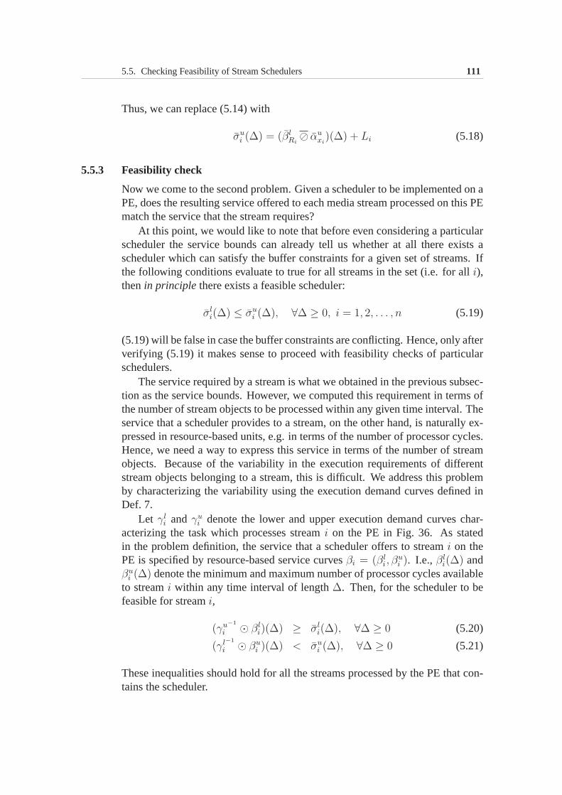
5.5. Checking Feasibility of Stream Schedulers 111
Thus, we can replace (5.14) with
σui (∆) = (βl
Ri⊘ αu
xi)(∆) + Li (5.18)
5.5.3 Feasibility check
Now we come to the second problem. Given a scheduler to be implemented on aPE, does the resulting service offered to each media stream processed on this PEmatch the service that the stream requires?
At this point, we would like to note that before even considering a particularscheduler the service bounds can already tell us whether at all there exists ascheduler which can satisfy the buffer constraints for a given set of streams. Ifthe following conditions evaluate to true for all streams inthe set (i.e. for alli),thenin principle there exists a feasible scheduler:
σli(∆) ≤ σu
i (∆), ∀∆ ≥ 0, i = 1, 2, . . . , n (5.19)
(5.19) will be false in case the buffer constraints are conflicting. Hence, only afterverifying (5.19) it makes sense to proceed with feasibilitychecks of particularschedulers.
The service required by a stream is what we obtained in the previous subsec-tion as the service bounds. However, we computed this requirement in terms ofthe number of stream objects to be processed within any giventime interval. Theservice that a scheduler provides to a stream, on the other hand, is naturally ex-pressed in resource-based units, e.g. in terms of the numberof processor cycles.Hence, we need a way to express this service in terms of the number of streamobjects. Because of the variability in the execution requirements of differentstream objects belonging to a stream, this is difficult. We address this problemby characterizing the variability using the execution demand curves defined inDef. 7.
Let γli andγu
i denote the lower and upper execution demand curves char-acterizing the task which processes streami on the PE in Fig. 36. As statedin the problem definition, the service that a scheduler offers to streami on thePE is specified by resource-based service curvesβi = (βl
i, βui ). I.e.,βl
i(∆) andβu
i (∆) denote the minimum and maximum number of processor cycles availableto streami within any time interval of length∆. Then, for the scheduler to befeasible for streami,
(γu−1
i ⊙ βli)(∆) ≥ σl
i(∆), ∀∆ ≥ 0 (5.20)
(γl−1
i ⊙ βui )(∆) < σu
i (∆), ∀∆ ≥ 0 (5.21)
These inequalities should hold for all the streams processed by the PE that con-tains the scheduler.
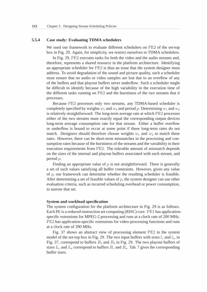
112 Chapter 5. Designing Stream Scheduling Policies
5.5.4 Case study: Evaluating TDMA schedulers
We used our framework to evaluate different schedulers onPE2 of the set-topbox in Fig. 29. Again, for simplicity, we restrict ourselvesto TDMA schedulers.
In Fig. 29,PE2 executes tasks for both the video and the audio streams and,therefore, represents a shared resource in the platform architecture. Identifyingan appropriate scheduler forPE2 is thus an issue that the system designer mustaddress. To avoid degradation of the sound and picture quality, such a schedulermust ensure that no audio or video samples are lost due to an overflow of anyof the buffers and that playout buffers never underflow. Sucha scheduler mightbe difficult to identify because of the high variability in the execution time ofthe different tasks running onPE2 and the burstiness of the two streams that itprocesses.
BecausePE2 processes only two streams, any TDMA-based scheduler iscompletely specified by weightsw1 andw2 and periodp. Determiningw1 andw2
is relatively straightforward. The long-term average rateat whichPE2 processeseither of the two streams must exactly equal the corresponding output deviceslong-term average consumption rate for that stream. Eithera buffer overflowor underflow is bound to occur at some point if these long-termrates do notmatch. Designers should therefore choose weightsw1 andw2 to match theserates. However, there can be short-term mismatches in the processing and con-sumption rates because of the burstiness of the streams and the variability in theirexecution requirements fromPE2. The tolerable amount of mismatch dependson the sizes of the internal and playout buffers associated with each stream, andperiodp.
Finding an appropriate value ofp is not straightforward. There is generallya set of such values satisfying all buffer constraints. However, given any valueof p, our framework can determine whether the resulting scheduler is feasible.After determining a set of feasible values ofp, the system designer can use otherevaluation criteria, such as incurred scheduling overheador power consumption,to narrow that set.
System and workload specificationThe system configuration for the platform architecture in Fig. 29 is as follows.Each PE is a reduced-instruction set computing (RISC) core.PE1 has application-specific extensions for MPEG-2 processing and runs at a clockrate of 200 MHz.PE2 has application-specific extensions for video-processingfunctions and runsat a clock rate of 390 MHz.
Fig. 37 shows an abstract view of processing elementPE2 in the systemmodel of the set-top box in Fig. 29. The two input buffers withsizeslv andla, inFig. 37, correspond to buffersB2 andB3 in Fig. 29. The two playout buffers ofsizesLv andLa correspond to buffersBv andBa. Tab. 7 gives the correspondingbuffer sizes.
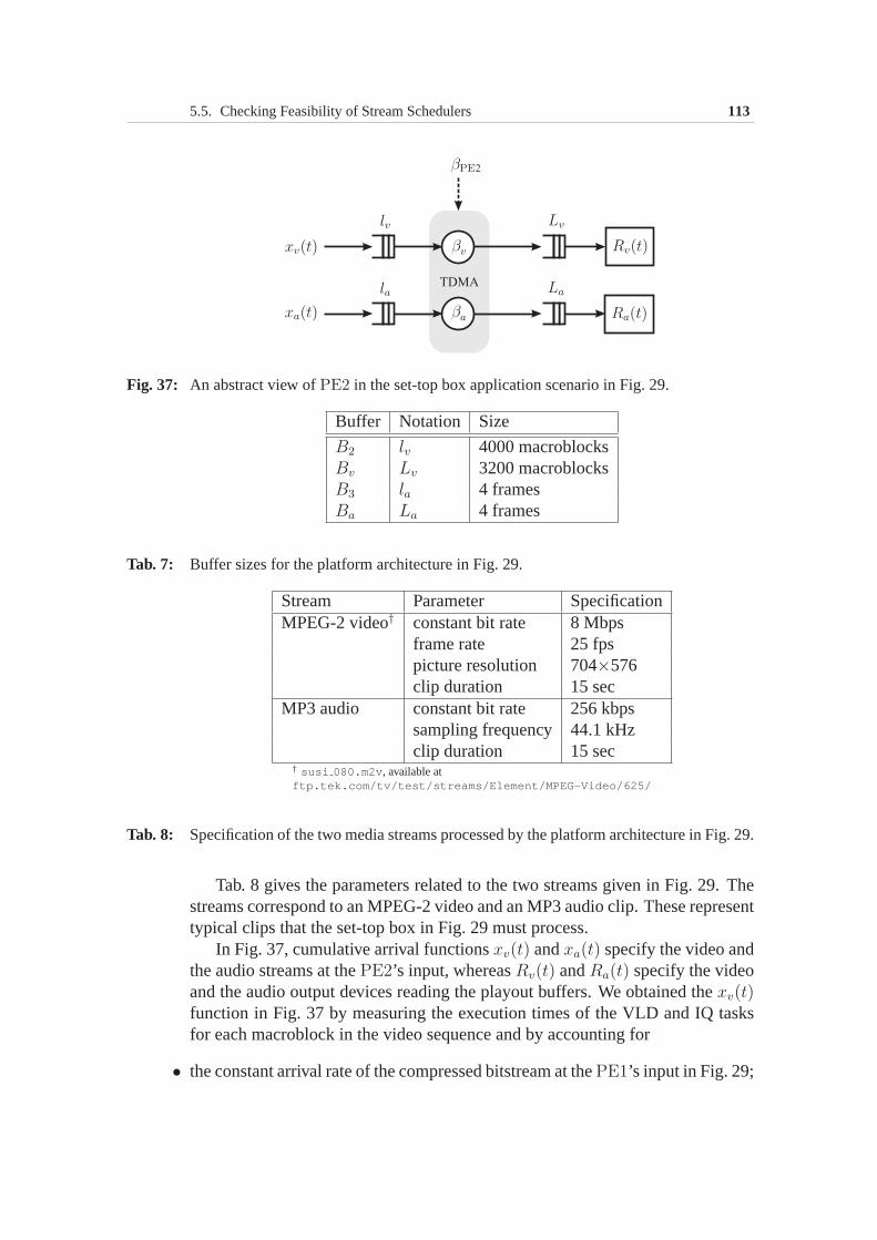
5.5. Checking Feasibility of Stream Schedulers 113
Fig. 37: An abstract view ofPE2 in the set-top box application scenario in Fig. 29.
Buffer Notation Size
B2 lv 4000 macroblocksBv Lv 3200 macroblocksB3 la 4 framesBa La 4 frames
Tab. 7: Buffer sizes for the platform architecture in Fig. 29.
Stream Parameter SpecificationMPEG-2 video† constant bit rate 8 Mbps
frame rate 25 fpspicture resolution 704×576clip duration 15 sec
MP3 audio constant bit rate 256 kbpssampling frequency 44.1 kHzclip duration 15 sec
† susi 080.m2v, available atftp.tek.com/tv/test/streams/Element/MPEG-Video/625/
Tab. 8: Specification of the two media streams processed by the platform architecturein Fig. 29.
Tab. 8 gives the parameters related to the two streams given in Fig. 29. Thestreams correspond to an MPEG-2 video and an MP3 audio clip. These representtypical clips that the set-top box in Fig. 29 must process.
In Fig. 37, cumulative arrival functionsxv(t) andxa(t) specify the video andthe audio streams at thePE2’s input, whereasRv(t) andRa(t) specify the videoand the audio output devices reading the playout buffers. Weobtained thexv(t)function in Fig. 37 by measuring the execution times of the VLD and IQ tasksfor each macroblock in the video sequence and by accounting for
• the constant arrival rate of the compressed bitstream at thePE1’s input in Fig. 29;

114 Chapter 5. Designing Stream Scheduling Policies
Fig. 38: Specification of the video stream: functionsxv(t) andRv(t) from Fig. 37.
and
• the number of bits per macroblock, which is variable becauseof the VLD task.
Further, in our setup,PE1 executed only the task performing the VLD and IQfunctions. I.e., the full processing capacity ofPE1 was devoted exclusively tothis task, and no scheduler, therefore, was employed to schedulePE1.
Fig. 38 shows the resulting function,xv(t). Similarly, functionRv(t), shownin Fig. 38, specifies the consumption of the video stream by video output device.The value of this function is0 for the first 0.34 seconds, corresponding to aplayout delay. After this delay, the function increases with a constant slope,representing a periodic consumption pattern of39.600 macroblocks per second.(One macroblock corresponds to a16 × 16 pixel block in a frame; thus, oneframe with resolution704 × 576 pixels contains1.584 macroblocks. Therefore,25 frames per second result in39.600 macroblocks per second.)
The execution demand curves shown in Fig. 39 capture the total executionrequirements of the task performing the IDCT and MC functionsonPE2. Ratherthan using a constant value, we use the execution demand curves to capture thevariation in the total execution requirements of this task.To obtain these curves,we first collected a trace of execution times for the task and then analyzed thistrace with the method described in Section 3.5.2.
Functionsxv(t) andRv(t), combined with the execution demand curves,completely specify the video stream. We obtain the specification of the audiostream similarly. Once such a specification of the streams isavailable, designerscan use our framework to evaluate any scheduler using the process in Fig. 30 andwithout resorting to further simulations.
Evaluating TDMA schedulers with different periodsGiven functionsxv, xa, Rv, andRa for the representative video and audio clips,Fig. 40 shows the service bounds,σl and σu, for the video and audio streams.
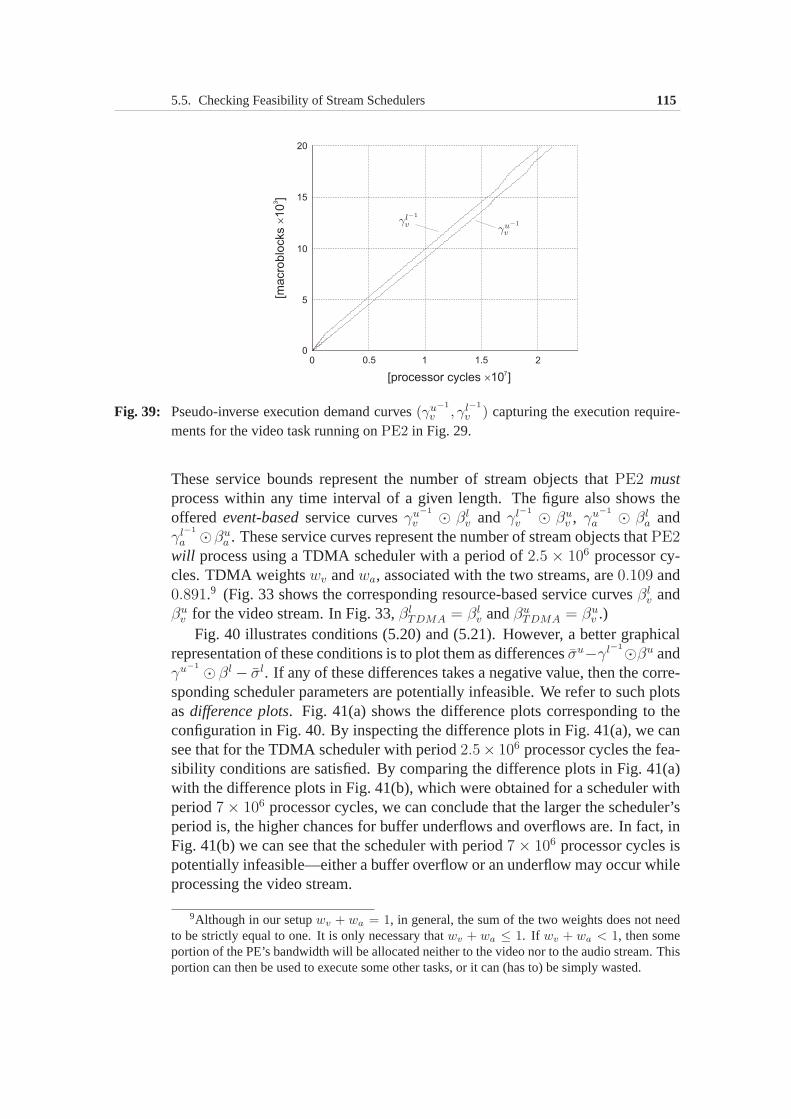
5.5. Checking Feasibility of Stream Schedulers 115
Fig. 39: Pseudo-inverse execution demand curves(γu−1
v , γl−1
v ) capturing the execution require-ments for the video task running onPE2 in Fig. 29.
These service bounds represent the number of stream objectsthat PE2 mustprocess within any time interval of a given length. The figurealso shows theoffered event-basedservice curvesγu−1
v ⊙ βlv and γl−1
v ⊙ βuv , γu−1
a ⊙ βla and
γl−1
a ⊙βua . These service curves represent the number of stream objects thatPE2
will process using a TDMA scheduler with a period of2.5 × 106 processor cy-cles. TDMA weightswv andwa, associated with the two streams, are0.109 and0.891.9 (Fig. 33 shows the corresponding resource-based service curvesβl
v andβu
v for the video stream. In Fig. 33,βlTDMA = βl
v andβuTDMA = βu
v .)Fig. 40 illustrates conditions (5.20) and (5.21). However,a better graphical
representation of these conditions is to plot them as differencesσu−γl−1⊙βu andγu−1 ⊙ βl − σl. If any of these differences takes a negative value, then thecorre-sponding scheduler parameters are potentially infeasible. We refer to such plotsasdifference plots. Fig. 41(a) shows the difference plots corresponding to theconfiguration in Fig. 40. By inspecting the difference plots in Fig. 41(a), we cansee that for the TDMA scheduler with period2.5× 106 processor cycles the fea-sibility conditions are satisfied. By comparing the difference plots in Fig. 41(a)with the difference plots in Fig. 41(b), which were obtainedfor a scheduler withperiod7 × 106 processor cycles, we can conclude that the larger the scheduler’speriod is, the higher chances for buffer underflows and overflows are. In fact, inFig. 41(b) we can see that the scheduler with period7 × 106 processor cycles ispotentially infeasible—either a buffer overflow or an underflow may occur whileprocessing the video stream.
9Although in our setupwv + wa = 1, in general, the sum of the two weights does not needto be strictly equal to one. It is only necessary thatwv + wa ≤ 1. If wv + wa < 1, then someportion of the PE’s bandwidth will be allocated neither to the video nor to the audio stream. Thisportion can then be used to execute some other tasks, or it can(has to) be simply wasted.

116 Chapter 5. Designing Stream Scheduling Policies
Fig. 40: Service requirements specified by service boundsσ and the actually provided servicespecified by curveγ−1 ⊙ β for the video (top) and audio (bottom) streams. The up-per and lower curves corresponding toγ−1 ⊙ β lie completely between the upper andlower service bounds,σ. This implies that the service provided to a stream matches itsrequirements; hence, the scheduler satisfies all the buffer constraints.For an infeasiblescheduler, the resulting upper and lower curves ofγ−1 ⊙ β would not completely liebetween the upper and lower curves ofσ.
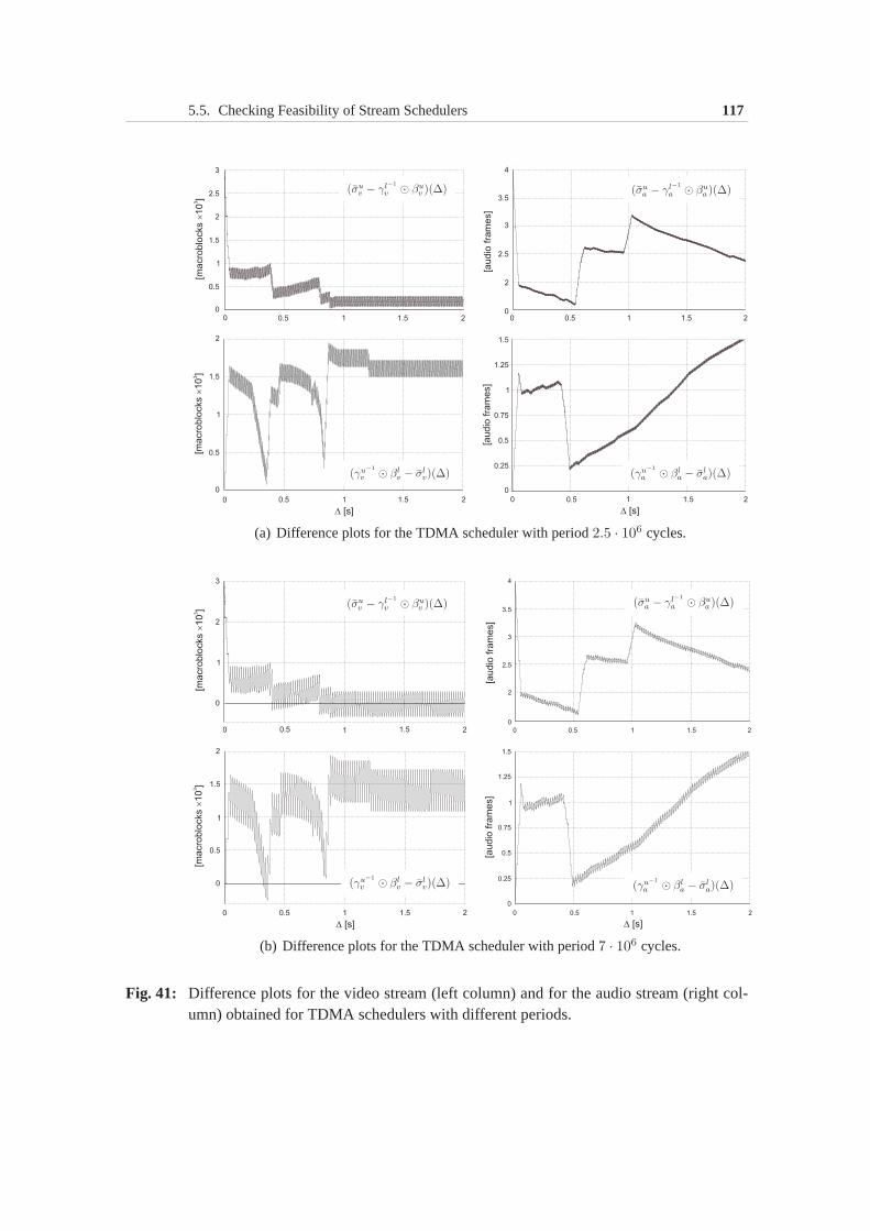
5.5. Checking Feasibility of Stream Schedulers 117
(a) Difference plots for the TDMA scheduler with period2.5 · 106 cycles.
(b) Difference plots for the TDMA scheduler with period7 · 106 cycles.
Fig. 41: Difference plots for the video stream (left column) and for the audio stream (right col-umn) obtained for TDMA schedulers with different periods.
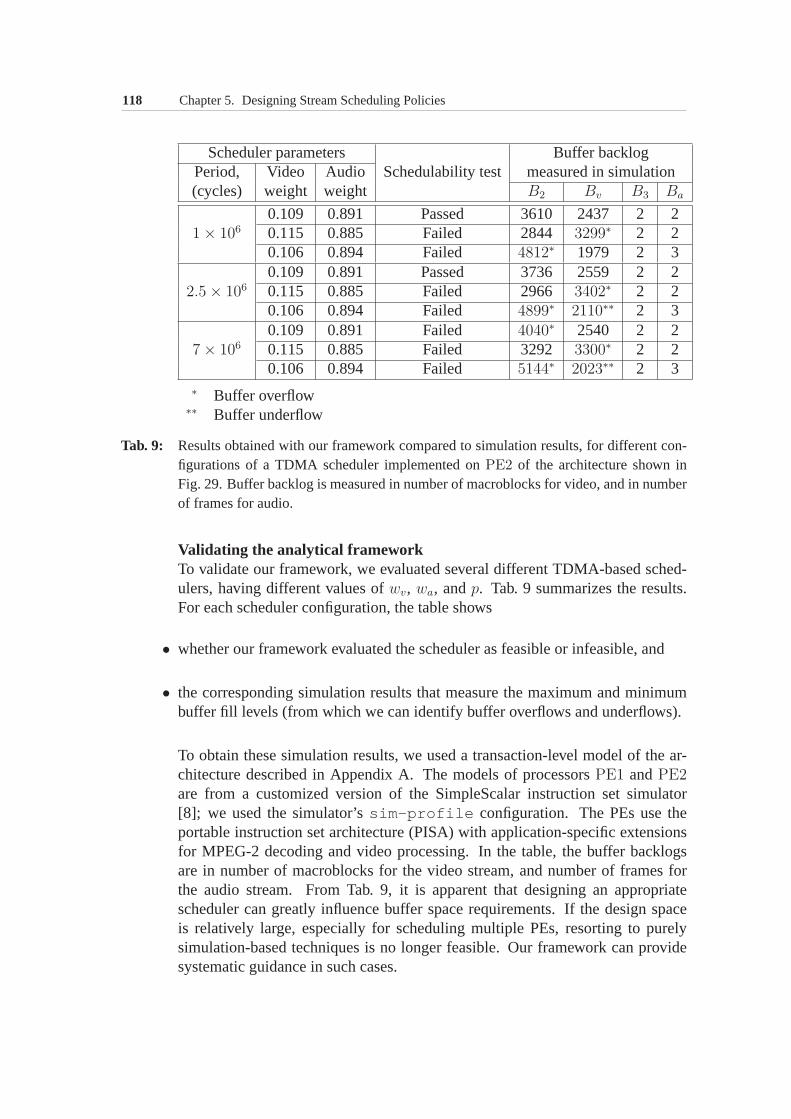
118 Chapter 5. Designing Stream Scheduling Policies
Scheduler parameters Buffer backlogPeriod, Video Audio Schedulability test measured in simulation(cycles) weight weight B2 Bv B3 Ba
0.109 0.891 Passed 3610 2437 2 21 × 106 0.115 0.885 Failed 2844 3299∗ 2 2
0.106 0.894 Failed 4812∗ 1979 2 30.109 0.891 Passed 3736 2559 2 2
2.5 × 10⁶ 0.115 0.885 Failed 2966 3402∗ 2 20.106 0.894 Failed 4899∗ 2110∗∗ 2 30.109 0.891 Failed 4040∗ 2540 2 2
7 × 10⁶ 0.115 0.885 Failed 3292 3300∗ 2 20.106 0.894 Failed 5144∗ 2023∗∗ 2 3
∗ Buffer overflow∗∗ Buffer underflow
Tab. 9: Results obtained with our framework compared to simulation results, for different con-figurations of a TDMA scheduler implemented onPE2 of the architecture shown inFig. 29. Buffer backlog is measured in number of macroblocks for video,and in numberof frames for audio.
Validating the analytical frameworkTo validate our framework, we evaluated several different TDMA-based sched-ulers, having different values ofwv, wa, andp. Tab. 9 summarizes the results.For each scheduler configuration, the table shows
• whether our framework evaluated the scheduler as feasible or infeasible, and
• the corresponding simulation results that measure the maximum and minimumbuffer fill levels (from which we can identify buffer overflows and underflows).
To obtain these simulation results, we used a transaction-level model of the ar-chitecture described in Appendix A. The models of processors PE1 andPE2are from a customized version of the SimpleScalar instruction set simulator[8]; we used the simulator’ssim-profile configuration. The PEs use theportable instruction set architecture (PISA) with application-specific extensionsfor MPEG-2 decoding and video processing. In the table, the buffer backlogsare in number of macroblocks for the video stream, and numberof frames forthe audio stream. From Tab. 9, it is apparent that designing an appropriatescheduler can greatly influence buffer space requirements.If the design spaceis relatively large, especially for scheduling multiple PEs, resorting to purelysimulation-based techniques is no longer feasible. Our framework can providesystematic guidance in such cases.
5.6. Summary 119
5.6 SummaryIn this chapter, we proposed a framework for design space exploration and opti-mization of platform management policies for multimedia MpSoC architectures.This framework relies on the VCC-based workload model and usesthe extendedMPA framework developed in Chapter 3. It features a combination of simu-lation and analytical performance evaluation phases. The simulation phase isperformed only once, before the design space exploration loop is started. Theoutcome of this phase is a set of VCCs capturing relevant workload character-istics. These VCCs are then used within the time-critical exploration loop forfast analytic performance evaluation and optimization of platform managementpolicies. The performance evaluation and optimization of the platform manage-ment policies rely on two techniques: The first technique computes upper boundon the buffer memory requirements associated with a given platform manage-ment policy, while the second technique allows for fast schedulability checksfor a given PE within the architecture. Both techniques account for the QoS re-quirements associated with processing media streams on buffer-constrained mul-tiprocessor architectures. The utility of the framework was demonstrated in thischapter through the case studies of a set-top box application scenario involvingthe TDMA scheduling policy.

120 Chapter 5. Designing Stream Scheduling Policies
6Energy-Efficient Stream Processing
Chapters 4 and 5 demonstrated applications of VCCs in system-level design ofmedia processors. Unlike these applications, where VCCs wereused in anoff-line setting, this chapter demonstrates anonline application of VCCs. “Onlineapplication” means that VCCs are used in a multimedia embeddedsystem whileit is operating, i.e. at run time. Based on the run-time information about theworkload, certain system parameters can be dynamically adapted such that tooptimally suit current user needs and to improve the qualityof service offeredby the system to its users. Reducing energy consumption of embedded systemsthrough online adaptations to the varying workload is one important incarnationof this basic idea. In this chapter, we explore this direction — we show howVCCs can be used to perform such adaptations to achieve energy savings inmedia processors. Although this chapter has a clear focus onthe energy-awareadaptations, the main concept behind the presented approach can be applied in abroader context of adaptive stream scheduling for real-time embedded systems.
The focus of this chapter is on a scheme for dynamic voltage scaling (DVS)for processing media streams on architectures with restricted buffer sizes. Themain advantage of this scheme is its ability to providehard QoS guaranteeswhile still achieving considerable energy savings. VCCs are central to the wholemethod. They allow to handle multimedia workloads characterized by both,the data-dependent variability in the execution time of multimedia tasks and theburstiness in the on-chip traffic arising out of multimedia processing. The mainnovelty of the scheme lies in a online DVS strategy which usesfor the adap-tationsdynamic VCCs, i.e. VCCs that are computed at run time based on the“conventional”static VCCsand the workload history. The DVS scheme is fullyscalable and has a bounded application-independent run-time overhead.
122 Chapter 6. Energy-Efficient Stream Processing
This chapter has the following structure:
• Section 6.1 introduces our DVS technique, outlining main differences to similarapproaches.
• Section 6.2 gives an overview of existing DVS techniques.
• Using a motivating example, Section 6.3 describes the problem addressed by ourmethod.
• Section 6.4 describes the method.
• Section 6.5 presents results of an experimental evaluationof the proposed DVStechnique, including a comparison with a similar method.
• Finally, some concluding remarks come at the end of this chapter, in Section 6.6.
6.1 IntroductionMultimedia applications constitute a significant portion of the workload runningon battery-powered devices such as PDAs, mobile phones and portable audio-video players [36, 77]. A major challenge faced by the designers of such devicesis the need for minimizing energy consumption and at the sametime handlingcomputationally expensive multimedia workloads and providing QoS guaran-tees. The bursty and highly irregular nature of such a workload, coupled withstringent memory and cost constraints associated with portable devices makesthis problem even more difficult.
One important research direction aimed at solving this problem relies on dy-namically changing the processor’s clock frequency and voltage in response toa time-varying workload [27]. This technique, called Dynamic Voltage Scaling(DVS), rests on the fact that reducing the supply voltage of CMOS circuits resultsin approximately quadratic reduction in dynamic energy dissipation. Althoughthis energy reduction does not come for free (a lower supply voltage leads toincreased gate delays), DVS is known to be more effective than another energysaving technique, called Dynamic Power Management (DPM) [16]. In contrastto DVS, DPM simply puts a processor into a low power state whenthe proces-sor is idle. With the availability of variable-voltage processors [3, 58, 60, 164],research on DVS scheduling techniques has gained a lot of momentum.
Govil et al. [46] proposed to look at different DVS scheduling techniquesfrom two perspectives: the way how those techniquespredict the workload andhow theysmoothit. In order to make a decision at which speed to run the proces-sor during next interval of time, a DVS scheduler first has to make some as-sumptions about the workload on this interval. Making such assumptions canbe regarded as predicting the future workload. On the other hand, workload
6.1. Introduction 123
smoothing refers to apolicy followed by the DVS scheduler while deciding theprocessor speed. The concrete decision is based on the assumptions about the fu-ture workload, while the policy is typically determined by the performance goalsand constraints associated with the application(s) executed on the processor.
One promising approach forsmoothing outthe workload is to employ buffers.This technique usually achieves considerable energy savings, but at the expenseof increased processing delay. Nevertheless, it is especially useful in a large classof multimedia applications, which can tolerate such delays.
Recently, a number of DVS techniques has appeared in the literature whichuse buffers for smoothing out the workload [49, 59, 104, 106,144, 174]. Thesetechniques can be broadly classified into three groups basedon the way how theyperform theworkload prediction. [49, 144] predict the future workload based onstochastic models. [106, 174] employ feedback control loops to track workloadchanges and extrapolate the future workload. [59, 104] relyon off-line worst-case characterization of tasks and statically use this characterization at run-timefor making conservative scheduling decisions (i.e. essentially they do not useprediction as such, but assume at any time that the worst case workload willhappen).
Although it has been shown that the above lines of work lead toconsiderableenergy savings, all of them still suffer from a number drawbacks. The schemesbased on stochastic prediction models and feedback controlloops are power-ful in handling workloads which are characterized by both, the data-dependentvariability in the execution time of multimedia tasks and the burstiness in the on-chip traffic arising out of multimedia processing. However,usually it is difficultto provide hard QoS guarantees with such schemes. On the other hand, schemesthat rely on worst-case characterization of the workload can provide hard QoSguarantees. However, they account only for the task execution time variability,assuming that real-time tasks arrive strictly periodically.
In this chapter, we present a DVS scheduling technique whichaddresses theabove mentioned shortcomings of the previous approaches. It takes into accountboth, the burstiness in a stream and the data-dependent variability in the exe-cution time of a task. On the other hand, our scheme offers a guaranteed QoSalong with energy savings that are comparable with those obtained by previousapproaches. Furthermore, one of the main assumptions made by many exist-ing DVS schemes has been the availability of large buffers. However, in reality,many portable devices have severe cost and memory constraints. We addressthis issue by targeting our DVS scheme specifically towardsbuffer-constrainedarchitectures.
Our scheme relies on an off-line analysis to determineboundson the variabil-ity of the workload associated with aclassof media streams. These bounds arerepresented by VCCs introduced in Chapter 3. At run-time, by using a boundedamount of history of the actually incurred workload, the VCCs obtained from theoff-line analysis are revised. Such revised VCCs, which we refer to asdynamic
124 Chapter 6. Energy-Efficient Stream Processing
VCCs, are then used to adjust the processor’s voltage and clock frequency. Thesedynamic VCCs can be much tighter than their respectivestatic VCCs, i.e. thoseVCCs obtained from the off-line analysis. At the same time, thedynamic VCCsare “safe” in terms of guaranteeing QoS constraints.
The main results of this chapter are:
• A strategy for online processor rate adaptations for energy-efficient processingof media streams on buffer-constrained architectures.
• A formalization of this strategy as an algorithm which employs dynamic VCCsto provide hard QoS guarantees to the processed media streams.
• An efficient algorithm for run-time computation of dynamic VCCs from staticVCCs using the workload history.
• An experimental evaluation of the resulting DVS scheme, including its compar-ison to another up-to-date DVS scheme [174] and an estimation of the run-timeoverhead.
Although we present our VCC-based DVS scheme in the context of asim-ple setup, where DVS is implemented on a single processor running a multime-dia task, it can also be applied to more involved architectures such as on-chipnetworks [17, 31, 79, 144] and multiple clock domain processors [64, 123, 138,174].
6.2 Related WorkAlthough dynamic voltage scaling emerged almost a decade ago (see, e.g. [21,46, 122, 170]), it still remains a very active research area (e.g [5, 59, 81, 144]).Early explorations of this technique were primarily directed towards non-real-time computing systems [46, 124, 170]. Later on, DVS schemeshave been devel-oped for real-time systems, including off-line and on-linescheduling algorithmsfor a single processor [55, 61, 87, 177], multiple processors [69, 107, 176, 180]and heterogeneous distributed platform architectures [4,47, 136]. Some DVSschemes were designed for hard real-time applications [69,90, 139, 142], whileothers targeted soft real-time applications [56, 178]. Yetanother class of DVStechniques were specifically devised for systems processing media streams [29,30, 59, 106, 143]. With constantly shrinking technology feature sizes, there isa growing concern about rapid increase in leakage power dissipation of CMOScircuits [2, 20], which cannot be reduced by scaling the supply voltage. Conse-quently, new research directions, reconsidering DVS techniques and combiningthem, for example, with adaptive body-biasing [73, 110], recently has started toappear in the literature [5, 66, 175].
6.2. Related Work 125
As mentioned before, it is useful to view different DVS schemes from twoperspectives: how they predict the workload and which policy they use to smoothit [46]. These characteristics are tightly related to the energy-performance trade-offs made in the system. For instance, tasks in non-real-time systems do nothave stringent timing constraints, therefore the prime concern of DVS schemesdeveloped for this kind of systems is to maintain someaveragelevel of perfor-mance (e.g. average task response times) while maximizing the energy savings[42, 46, 124, 145, 170]. Since these DVS schemes do not need toprovide hardperformance guarantees, they allow for some inaccuracy in the workload pre-dictions. Hence, these schemes rely on different sorts of statistics for predict-ing the workload. [46, 124, 170] propose and experimentallyevaluate variousDVS schemes which calculate how busy the processor was during a number ofpast intervals and then apply various techniques, such as a weighted average, topredict the future workload from these calculations. [145]extends the work in[46, 124, 170] by introducing a concept ofworkload history filteringand propos-ing several prediction strategies based on this concept. [42] further improves theabove workload prediction mechanisms by taking into consideration activitiesof individual tasks. The majority of the DVS schemes just described employrelatively simple smoothing policies, such as setting the processor speed highenough to complete the predicted work before next adaptation point in time [46].
In hard real-time systems, guaranteeing that tasks complete within their dead-lines is of prime concern [22]. Consequently, DVS schemes forhard real-timesystems employ notably different mechanisms than those used in non-real-timesystems. In particular, since hard performance guaranteeshave to be provided,such DVS schemes cannot rely on statistics to predict the future workload. Infact, they perform a kind of degenerate form of prediction—at any time theseDVS schemes assume that theworst-caseworkload will happen. Hence, theyfully rely on worst-case characterization of tasks. As in traditional real-timescheduling [100], most of the DVS techniques designed for hard real-time sys-tems characterize tasks by their worst-case execution time(WCET) andexplicitlydefined arrival times and deadlines. Since such a characterization is inherentlystatic, the only mechanism which these DVS schemes can use at run time to savethe energy is the workload smoothing.
The main challenge in hard real-time scheduling of variable-voltage proces-sors is to smooth the workload as much as possible but still toguarantee thatall tasks complete within their deadlines. The workload smoothing is equivalentto increasing the processor utilization by minimizing theworst-case slack time(WST) and theworkload-variation slack time(VST) [90]. The worst-case slacktime is the time during which the processor is idle even if alltasks run at theirWCET. It is inherent to many real-time schedules. The workload-variation slacktime is the idle time which occurs as a result of tasks not always running at theirWCET. Different DVS techniques for hard real-time systems differ in the wayhow they exploit these two kinds of slack time and what assumptions they make
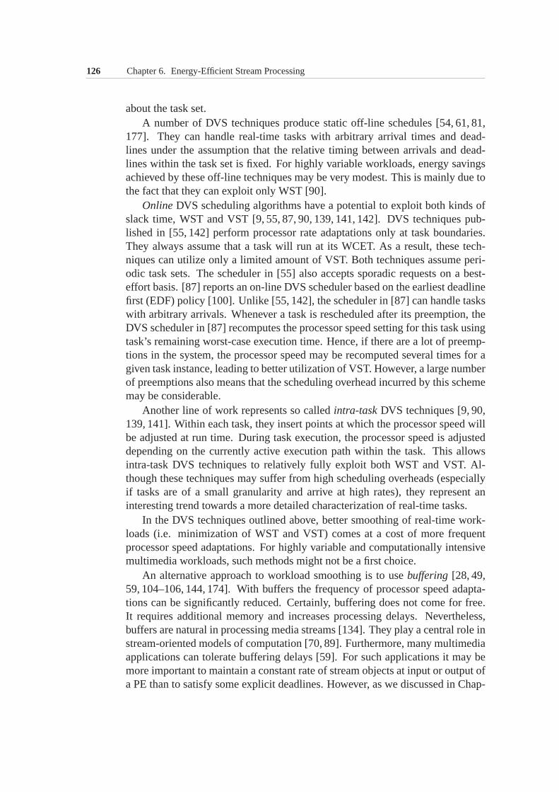
126 Chapter 6. Energy-Efficient Stream Processing
about the task set.A number of DVS techniques produce static off-line schedules [54, 61, 81,
177]. They can handle real-time tasks with arbitrary arrival times and dead-lines under the assumption that the relative timing betweenarrivals and dead-lines within the task set is fixed. For highly variable workloads, energy savingsachieved by these off-line techniques may be very modest. This is mainly due tothe fact that they can exploit only WST [90].
OnlineDVS scheduling algorithms have a potential to exploit both kinds ofslack time, WST and VST [9, 55, 87, 90, 139, 141, 142]. DVS techniques pub-lished in [55, 142] perform processor rate adaptations onlyat task boundaries.They always assume that a task will run at its WCET. As a result, these tech-niques can utilize only a limited amount of VST. Both techniques assume peri-odic task sets. The scheduler in [55] also accepts sporadic requests on a best-effort basis. [87] reports an on-line DVS scheduler based onthe earliest deadlinefirst (EDF) policy [100]. Unlike [55, 142], the scheduler in [87] can handle taskswith arbitrary arrivals. Whenever a task is rescheduled after its preemption, theDVS scheduler in [87] recomputes the processor speed setting for this task usingtask’s remaining worst-case execution time. Hence, if there are a lot of preemp-tions in the system, the processor speed may be recomputed several times for agiven task instance, leading to better utilization of VST. However, a large numberof preemptions also means that the scheduling overhead incurred by this schememay be considerable.
Another line of work represents so calledintra-taskDVS techniques [9, 90,139, 141]. Within each task, they insert points at which the processor speed willbe adjusted at run time. During task execution, the processor speed is adjusteddepending on the currently active execution path within thetask. This allowsintra-task DVS techniques to relatively fully exploit bothWST and VST. Al-though these techniques may suffer from high scheduling overheads (especiallyif tasks are of a small granularity and arrive at high rates),they represent aninteresting trend towards a more detailed characterization of real-time tasks.
In the DVS techniques outlined above, better smoothing of real-time work-loads (i.e. minimization of WST and VST) comes at a cost of morefrequentprocessor speed adaptations. For highly variable and computationally intensivemultimedia workloads, such methods might not be a first choice.
An alternative approach to workload smoothing is to usebuffering [28, 49,59, 104–106, 144, 174]. With buffers the frequency of processor speed adapta-tions can be significantly reduced. Certainly, buffering does not come for free.It requires additional memory and increases processing delays. Nevertheless,buffers are natural in processing media streams [134]. Theyplay a central role instream-oriented models of computation [70, 89]. Furthermore, many multimediaapplications can tolerate buffering delays [59]. For such applications it may bemore important to maintain a constant rate of stream objectsat input or output ofa PE than to satisfy some explicit deadlines. However, as we discussed in Chap-
6.2. Related Work 127
ter 5, buffer overflows and underflows may be of concern for this processingstyle.
One of the first DVS schemes employing buffers has appeared in[49]. AFIFO buffer is placed at the input of a PE whose clock rate and voltage are tobe regulated. The DVS scheme computes a moving average of theexecutiondemand to estimate the minimum sufficient processing rate for the samples cur-rently in the buffer. This technique assumes that exact execution demands ofindividual samples are knowna priori, i.e. before they have been processed.Only under this critical assumption and for periodic arrivals, the DVS scheme in[49] can guarantee absence of buffer over- and underflows. Based on the sameassumptions, [28] improves the rate estimation algorithm of [49] by extending itto the case when the selection of operating frequency/voltage levels is limited toa set of discrete values.
[104] proposes to insert buffers between tasks processing avideo stream ina pipelined fashion on a single PE. The buffers serve to maintain a constant out-put rate while allowing energy savings on a processor that has only few fixedfrequency levels. In addition, inserting the buffers improves response timesfor sporadic tasks executed on the same processor. [104] constructs frequency-assignment graphs capturing relevant information such as buffer states, and thendevelops efficient graph-walking algorithms to to find optimal frequency/voltagesettings at run time. It assumes that all frames to be processed are available atthe start of the operation (e.g. stored in memory or on a hard disk) and that thetasks have constant execution demands.
[59] shows that hard real-time DVS techniques not employingbuffers cannotfully utilize VST and therefore there is a potential to achieve higher energy sav-ings. To fully exploit both kinds of slack time, WST and VST, [59] proposes touse buffers to delay the processing such that whenever the processor has com-pleted execution of one task instance, italwaysfinds next task instance waitingin a buffer. Hence, if a preceding task instance has finished earlier than its WCETresulting in a slack time, then the next task instance is ableto fully utilize thisslack time while running at a lower clock rate. To guarantee that the buffersnever overflow and underflow, [59] has to assume that tasks arrivals are purelyperiodic.
In order to give the performance guarantees, DVS techniquesin [28, 49, 59,104] have to assume either periodic arrivals or, even worse,a completea prioriknowledge of the workload. These assumptions rarely hold inpractice. Otherbuffer-based DVS schemes published in [105, 106, 144, 174] are free from theseassumptions, however, as we will see, they fail to provide hard performanceguarantees.
[144] presents a buffer-based combined DVS-DPM scheme which fully relieson stochastic workload characterization: stream arrivalsand execution demandsare characterized by probability distributions. These distributions are obtainedby fitting statistics collected through extensive stochastic simulations to standard
128 Chapter 6. Energy-Efficient Stream Processing
Fig. 42: MPEG-2 decoder implemented on two PEs. Supply voltage and clock rate ofPE2 can becontrolled (DVS).x(t) ande(k) are cumulative arrival and execution demand functions.
probability distributions. At run time the workload history is collected and usedto detect, on the basis of these distributions, changes in the workload intensity.The processor rate is then adjusted accordingly. Clearly, due to its use of sto-chastic models the method in [144] can provide only probabilistic guarantees. Italso depends on the accuracy with which real workload is approximated usingstandard probability distributions.
DVS schemes presented in [105, 106, 144, 174] use different flavors of a PID(Proportional-Integral-Derivative) controller [37] to regulate the processor rate.The processor with the buffer at its input (or output) represents the controlledplant. Typically, the buffer occupancy level serves as a feedback signal to thecontroller. The main difficulty in these techniques is non-linearity of the con-trolled plant. Because of this non-linearity, it becomes extremely difficult toformally proof the properties of a control algorithm and analytically find op-timal settings for its parameters (such as controller gains). Furthermore, pro-viding hard performance guarantees (e.g. with respect to the buffer and delayconstraints) under highly bursty workloads requires an overshoot-free controllerwith a short reaction time. However, such a controller is difficult to design be-cause the requirements to have a short response time and to completely avoidovershoots are conflicting.
6.3 Motivating example
As a motivating example consider the system shown in Fig. 42.(A similar sys-tem has been already considered in Chapter 3 in Fig. 17 and in Chapter 4.) Thissystem performs decoding of MPEG-2 video streams. It includes two process-ing elementsPE1 andPE2. They can be embedded processor cores specializedfor specific tasks such as video processing or any other kind of processing ele-ments. A compressed video stream first entersPE1, which executes a part of theMPEG-2 decoding algorithm. The task running onPE1 performs VLD and IQfunctions. After processing onPE1, the video stream enters bufferB at PE2’s
6.3. Motivating example 129
input. At this place in the system the stream exists as a sequence of partiallydecodedmacroblocks. PE2 consumes fromB one macroblock at a time andapplies to it IDCT and MC functions. Finally, the fully decoded video streamemerges atPE2’s output.
Our objective is to minimize the energy consumed byPE2 without deteriorat-ing the quality of the processed video stream. The stream’s quality is preservedif bufferB at thePE2’s input never overflows and if the processing delay, experi-enced by the stream onPE2, does not exceed some specified value. Our ultimategoal is to design apredictable system. This means that we want to ensure that thesystem satisfies the above mentioned QoS requirements underall possible loadscenarios and not only in the average case.
We assume thatPE2 supports DVS, i.e. its clock rate and supply voltage canbe changed at run time.1 Such changes can be controlled by the software onPE2or by some other hardware or software entity, external toPE2. We refer to timeinstants at which the processor speed is altered asadaptation points.
We assume that the adaptation points are fixed in time. For obtaining en-ergy savings while providing the QoS guarantees, such an assumption is lessfavorable than the assumption that we can adapt the processor’s clock rate at anytime. Our method though can handle both cases. In any case, the spacing ofthe adaptation points in time in our method is completely decoupled from theexecution state and granularity of tasks onPE2. This means that the adaptationsare not restricted to occur at task boundaries, and their frequency, in general, isindependent of the rate at which the video stream arrives at thePE2’s input.
A DVS scheduler can reduce the energy dissipated onPE2 by exploiting thevariability of the workload imposed on this PE. This variability comes from twosources. First, the execution time of the task running onPE2 is variable. Second,the data-dependent variability of the execution time of thetask running onPE1causes the stream of macroblocks at thePE2’s input to bebursty.
One traditional way of reducing the energy dissipated onPE2 would be tofully average out the workload imposed on it using bufferB. If buffer B is suf-ficiently large, it can completely absorb the workload fluctuations. This allowsPE2 to run at a lowconstantclock rate which is just sufficient to sustain thelong-term average arrival rate of the stream. In this mode, one can ensure thatBnever gets empty (as a playout buffer). In this case, no cycles are wasted evenduring low-load periods, i.e. the available slack isfully exploited. This strategywould yield the most energy savings onPE2. However, such a strategy is of-ten unaffordable since it requires large buffers for processing bursty multimediaworkloads like MPEG streams. As an example, our experimentsshowed that thecomplete averaging of the workload imposed by DVD-quality videos onPE2 inFig. 42 required in the worst case the buffer space of at least8100 macroblocks(or about 3.7 MByte). Such a large buffer would be too expensive to imple-
1Throughout this chapter whenever we say that the processor’s rate is changed we assumethat to reduce energy its supply voltage is changed accordingly.
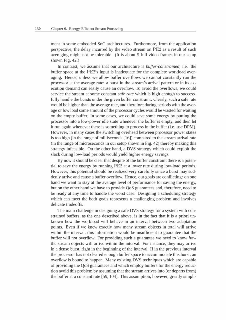
130 Chapter 6. Energy-Efficient Stream Processing
ment in some embedded SoC architectures. Furthermore, fromthe applicationperspective, the delay incurred by the video stream onPE2 as a result of suchaveraging might not be tolerable. (It is about 5 full video frames in our setupshown Fig. 42.)
In contrast, we assume that our architecture isbuffer-constrained, i.e. thebuffer space at thePE2’s input is inadequate for the complete workload aver-aging. Hence, unless we allow buffer overflows we cannot constantly run theprocessor at the average rate: a burst in the stream’s arrival pattern or in its ex-ecution demand can easily cause an overflow. To avoid the overflows, we couldservice the stream at some constantsafe ratewhich is high enough to success-fully handle the bursts under the given buffer constraint. Clearly, such a safe ratewould be higher than the average rate, and therefore during periods with the aver-age or low load some amount of the processor cycles would be wasted for waitingon the empty buffer. In some cases, we could save some energy by putting theprocessor into a low-power idle state whenever the buffer isempty, and then letit run again whenever there is something to process in the buffer (i.e. use DPM).However, in many cases the switching overhead between processor power statesis too high (in the range of milliseconds [16]) compared to the stream arrival rate(in the range of microseconds in our setup shown in Fig. 42) thereby making thisstrategy infeasible. On the other hand, a DVS strategy whichcould exploit theslack during low-load periods would yield higher energy savings.
By now it should be clear that despite of the buffer constraintthere is a poten-tial to save the energy by runningPE2 at a lower rate during low-load periods.However, this potential should be realized very carefully since a burst may sud-denly arrive and cause a buffer overflow. Hence, our goals areconflicting: on onehand we want to stay at the average level of performance for saving the energy,but on the other hand we have to provide QoS guarantees and, therefore, need tobe ready at any time to handle the worst case. Designing a scheduling strategywhich can meet the both goals represents a challenging problem and involvesdelicate tradeoffs.
The main challenge in designing a safe DVS strategy for a system with con-strained buffers, as the one described above, is in the fact that it is a priori un-known how the workload will behave in an interval between twoadaptationpoints. Even if we knew exactly how many stream objects in total will arrivewithin the interval, this information would be insufficientto guarantee that thebuffer will not overflow. For providing such a guarantee we need to knowhowthe stream objects will arrive within the interval. For instance, they may arrivein a dense burst, right in the beginning of the interval. If inthe previous intervalthe processor has not cleared enough buffer space to accommodate this burst, anoverflow is bound to happen. Many existing DVS techniques which are capableof providing the QoS guarantees and which employ buffers forthe energy reduc-tion avoid this problem by assuming that the stream arrives into (or departs from)the buffer at a constant rate [59, 104]. This assumption, however, greatly simpli-
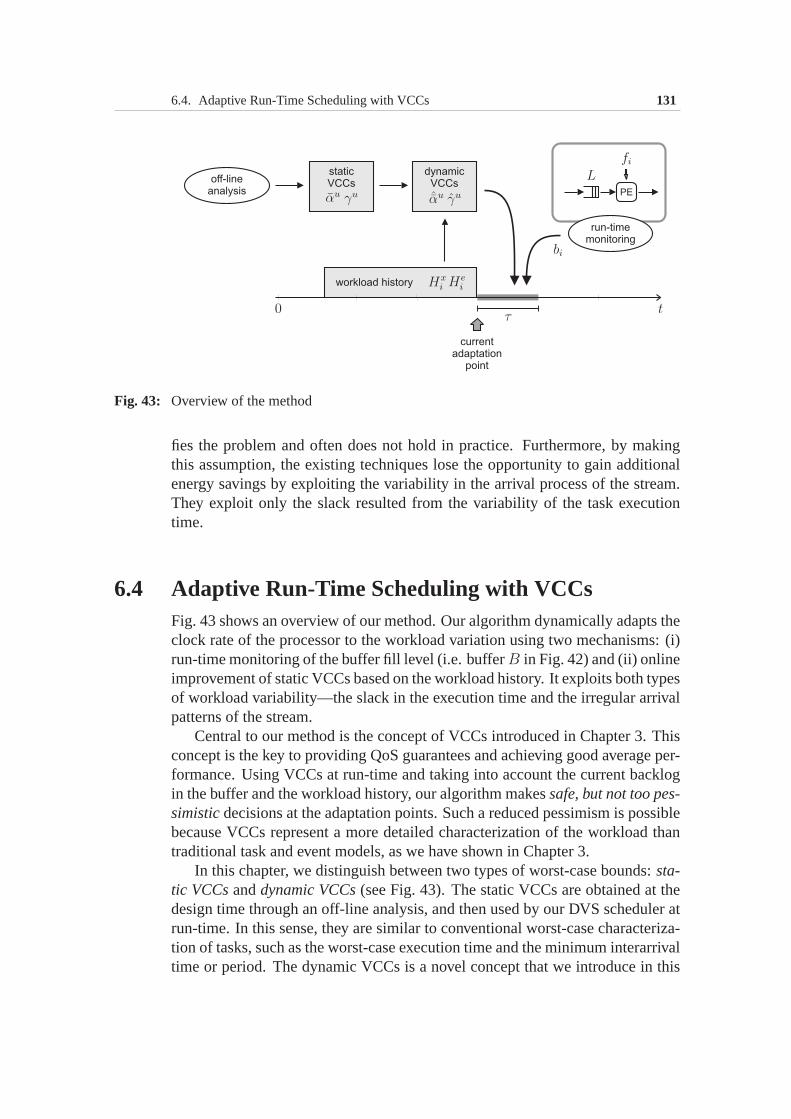
6.4. Adaptive Run-Time Scheduling with VCCs 131
Fig. 43: Overview of the method
fies the problem and often does not hold in practice. Furthermore, by makingthis assumption, the existing techniques lose the opportunity to gain additionalenergy savings by exploiting the variability in the arrivalprocess of the stream.They exploit only the slack resulted from the variability ofthe task executiontime.
6.4 Adaptive Run-Time Scheduling with VCCsFig. 43 shows an overview of our method. Our algorithm dynamically adapts theclock rate of the processor to the workload variation using two mechanisms: (i)run-time monitoring of the buffer fill level (i.e. bufferB in Fig. 42) and (ii) onlineimprovement of static VCCs based on the workload history. It exploits both typesof workload variability—the slack in the execution time andthe irregular arrivalpatterns of the stream.
Central to our method is the concept of VCCs introduced in Chapter3. Thisconcept is the key to providing QoS guarantees and achievinggood average per-formance. Using VCCs at run-time and taking into account the current backlogin the buffer and the workload history, our algorithm makessafe, but not too pes-simisticdecisions at the adaptation points. Such a reduced pessimism is possiblebecause VCCs represent a more detailed characterization of the workload thantraditional task and event models, as we have shown in Chapter3.
In this chapter, we distinguish between two types of worst-case bounds:sta-tic VCCsanddynamic VCCs(see Fig. 43). The static VCCs are obtained at thedesign time through an off-line analysis, and then used by our DVS scheduler atrun-time. In this sense, they are similar to conventional worst-case characteriza-tion of tasks, such as the worst-case execution time and the minimum interarrivaltime or period. The dynamic VCCs is a novel concept that we introduce in this
132 Chapter 6. Energy-Efficient Stream Processing
chapter. The novelty of this concept lies in the fact that these VCCs are ob-tainedat run-time. They represent an online improvement of the static VCCs.The dynamic VCCs are obtained using the workload history. Depending on theworkload situation, these VCCs can be much tighter than the corresponding staticVCCs. They allow our scheduler to be less pessimistic about thefuture work-load and through this to achieve considerable energy savings. Furthermore, thedynamic VCCs provide the same level of guarantee as that provided by the staticVCCs from which these dynamic VCCs were derived.
Following subsections give details about our method.
6.4.1 Workload and service characterization
We shall consider a stream to be composed of a potentially infinite sequence ofstream objects. Depending on the application at hand a stream object can bean audio sample, a video (macro)block or a whole frame, etc. Astream can bemodeled by two cumulative functionsx(t) ande(k) (see Fig. 42).x(t) denotesthe total number of stream objects that arrived at the bufferB during the time in-terval[0, t], wherease(k) denotes the total number of execution cycles requestedfrom the processor byk consecutive stream objects starting from the first streamobject in the sequence. Our objective is to characterize a whole classof streamsthat the processor has to handle. We achieve this by using upper event-basedarrival curveαu and upper execution demand curveγu, defined in Section 3.3.For any streami belonging to the class,αu andγu have to satisfy
xi(t+ ∆) − xi(t) ≤ αu(∆) ∀t,∆ ∈ R≥0 (6.1)
ei(k + ǫ) − ei(k) ≤ γu(ǫ) ∀k, ǫ ∈ Z>0 (6.2)
Thus, tuple(αu, γu) represents a particular class of streams. In practice, a classmay encompass all streams belonging to one application scenario. For instance,all MPEG-2 video sequences with identical parameters like resolution, framerate, bit rate etc. can belong to one class.
Besides the workload model represented by the arrival and execution demandcurves, we need a similar abstraction for the service offered to process this work-load. Note that the rate of a DVS processor can change over time. Hence, wehave to model these changes properly. For this we use the concept of aservicecurves. The theoretical framework presented in this chapter involves both, event-based and resource-based lower service curves, denotedβl andβl, respectively.In the simplest case, when the processor constantly runs at aclock ratef , theservice curveβl(∆) = f · ∆. For a processor which may be switched off formaximumδ time units and in the rest of the time runs at a constant speedf , e.g.as in the case of DPM,βl(∆) = sup{f · (∆ − δ), 0}.
6.4. Adaptive Run-Time Scheduling with VCCs 133
6.4.2 Safe service rate
To simplify exposition of the method, we introduce the concept of safe servicerate and make the following assumption: all stream objects in a stream imposethe same execution demand on the processor. This assumptionimplies that ifthe processor clock rate is constant on some time interval, then the service ratemeasured in number of stream objects per time unit which the processor offers tothe stream is also constant on that interval. We will relax this assumption later,in Section 6.4.4, by accounting for the execution demand variability.
Def. 16: (Safe service rate)Service rate is safe ifcontinuouslyservicing a stream at thisrate guarantees that the buffer at the input of the processornever overflows andthe delay constraint associated with the processed stream issatisfied.
Our goal is to determine theminimumsafe rate. For this, suppose that theprocessor services a stream at aconstantrateR, whereR is measured in numberof stream objects that can be serviced per time unit. Hence, we can model theoffered service asβl(∆) = R · ∆. Then, from (2.10) we can find the minimumservice rateRL which ensures that the buffer of sizeL never overflows:
RL = sup∀∆≥0
{
αu(∆) − L
∆
}
(6.3)
Similarly, from (2.9) we can determine the minimum service rateRD satisfyingthe delay constraintD:
RD = sup∀∆≥0
{
αu(∆)
D + ∆
}
(6.4)
Thus, the minimum safe service rateRsafe = max{RL, RD}, i.e.
Rsafe = sup∀∆∈R≥0
{
αu(∆)
D + ∆,αu(∆) − L
∆
}
(6.5)
To guarantee satisfaction of the buffer and delay constraints,L andD, it issufficient (but not necessary) that the processor offers a service rate which isnot lower thanRsafe determined by (6.5). In other words,Rsafe guarantees theconstraint satisfaction in the worst case, e.g. during a burst in the stream arrivalpattern. However, the appearance of the worst case is bounded, and therefore it isnot necessary for the processor to offer to the stream a safe service rate throughall the time. Whenever the worst case does not happen, the processor could offera service rate which is lower than the minimum safe rate. In doing so, care mustbe taken to timely react to changes in the workload by increasing the servicerate if necessary. This principle forms a basis for the dynamic processor rateadaptations which we will consider in the next subsection.
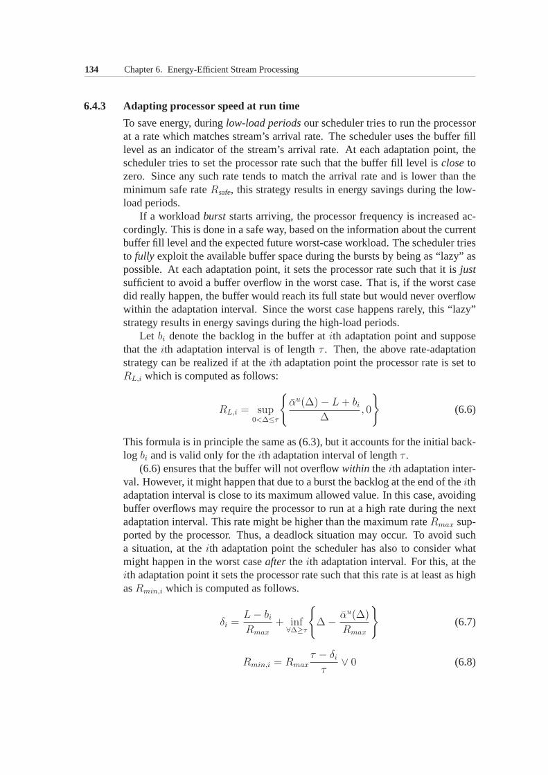
134 Chapter 6. Energy-Efficient Stream Processing
6.4.3 Adapting processor speed at run time
To save energy, duringlow-load periodsour scheduler tries to run the processorat a rate which matches stream’s arrival rate. The scheduleruses the buffer filllevel as an indicator of the stream’s arrival rate. At each adaptation point, thescheduler tries to set the processor rate such that the buffer fill level is closetozero. Since any such rate tends to match the arrival rate and is lower than theminimum safe rateRsafe, this strategy results in energy savings during the low-load periods.
If a workloadburst starts arriving, the processor frequency is increased ac-cordingly. This is done in a safe way, based on the information about the currentbuffer fill level and the expected future worst-case workload. The scheduler triesto fully exploit the available buffer space during the bursts by being as “lazy” aspossible. At each adaptation point, it sets the processor rate such that it isjustsufficient to avoid a buffer overflow in the worst case. That is, if the worst casedid really happen, the buffer would reach its full state but would never overflowwithin the adaptation interval. Since the worst case happens rarely, this “lazy”strategy results in energy savings during the high-load periods.
Let bi denote the backlog in the buffer atith adaptation point and supposethat theith adaptation interval is of lengthτ . Then, the above rate-adaptationstrategy can be realized if at theith adaptation point the processor rate is set toRL,i which is computed as follows:
RL,i = sup0<∆≤τ
{
αu(∆) − L+ bi∆
, 0
}
(6.6)
This formula is in principle the same as (6.3), but it accounts for the initial back-log bi and is valid only for theith adaptation interval of lengthτ .
(6.6) ensures that the buffer will not overflowwithin theith adaptation inter-val. However, it might happen that due to a burst the backlog at the end of theithadaptation interval is close to its maximum allowed value. In this case, avoidingbuffer overflows may require the processor to run at a high rate during the nextadaptation interval. This rate might be higher than the maximum rateRmax sup-ported by the processor. Thus, a deadlock situation may occur. To avoid sucha situation, at theith adaptation point the scheduler has also to consider whatmight happen in the worst caseafter the ith adaptation interval. For this, at theith adaptation point it sets the processor rate such that thisrate is at least as highasRmin,i which is computed as follows.
δi =L− biRmax
+ inf∀∆≥τ
{
∆ − αu(∆)
Rmax
}
(6.7)
Rmin,i = Rmax
τ − δiτ
∨ 0 (6.8)
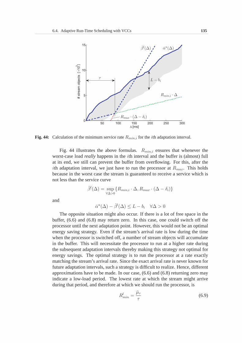
6.4. Adaptive Run-Time Scheduling with VCCs 135
Fig. 44: Calculation of the minimum service rateRmin,i for theith adaptation interval.
Fig. 44 illustrates the above formulas.Rmin,i ensures that whenever theworst-case loadreally happens in theith interval and the buffer is (almost) fullat its end, we still can prevent the buffer from overflowing. For this, after theith adaptation interval, we just have to run the processor atRmax. This holdsbecause in the worst case the stream is guaranteed to receivea service which isnot less than the service curve
βl(∆) = sup∀∆>0
{Rmin,i · ∆, Rmax · (∆ − δi)}
andαu(∆) − βl(∆) ≤ L− bi ∀∆ > 0
The opposite situation might also occur. If there is a lot of free space in thebuffer, (6.6) and (6.8) may return zero. In this case, one could switch off theprocessor until the next adaptation point. However, this would not be an optimalenergy saving strategy. Even if the stream’s arrival rate islow during the timewhen the processor is switched off, a number of stream objects will accumulatein the buffer. This will necessitate the processor to run at ahigher rate duringthe subsequent adaptation intervals thereby making this strategy not optimal forenergy savings. The optimal strategy is to run the processorat a rate exactlymatching the stream’s arrival rate. Since the exact arrivalrate is never known forfuture adaptation intervals, such a strategy is difficult torealize. Hence, differentapproximations have to be made. In our case, (6.6) and (6.8) returning zero mayindicate a low-load period. The lowest rate at which the stream might arriveduring that period, and therefore at which we should run the processor, is
Rlmin =
µτ
τ(6.9)
136 Chapter 6. Energy-Efficient Stream Processing
whereµτ denotes the minimum number of stream objects that might arrive withinany interval of lengthτ . 2
Finally, our algorithm can be summarized as follows:
Ri = max{RL,i, Rmin,i, Rlmin, RD} (6.10)
whereRi is the rate set at theith adaptation point.
6.4.4 Accounting for variable execution demand
The above discussion was based on the assumption that all stream objects im-pose exactly the same execution demand on the processor. Although in realitythis rarely happens, this assumption helped to illustrate the principles of the pro-posed rate adaptation algorithm by simplifying the formulation of the servicerate constraints in the preceding subsections. However, ifwe were to apply thisassumption in practice, we would also have to assume theworst-caseexecu-tion demand for each stream object. As our experiments showed in Section 3.6,such an assumption may result in overly pessimistic bounds.Therefore, to avoidthis problem, our method employs the upper execution demandcurveγu, whichrepresents a more detailed characterization of the worst-case execution demandimposed by a stream on the processor.
As discussed in Section 3.4, the workload transformation(γu ⊙ αu)(∆) givesan upper bound on the number of processor cycles that can be requested withinany time interval of length∆ by any stream belonging to the class characterizedby tuple(αu, γu). Using this workload transformation and Thm. 1, and by fol-lowing the same principles as were used for deriving (6.4), (6.6), and (6.8), wecan obtain constraints on the processorclockrate:
fD = sup∀∆≥0
{
γu ⊙ αu(∆)
D + ∆
}
(6.11)
fL,i = sup0<∆≤τ
{
γu ⊙ ((αu(∆) − L+ bi) ∨ 0))
∆
}
(6.12)
fmin,i = sup∀∆≥τ
{
fmax(τ − ∆) + γu ⊙ ((αu(∆) − L+ bi) ∨ 0)
τ
}
(6.13)
wherefD, fL,i andfmin,i are clock frequencies, corresponding to event-basedservice ratesRD, RL,i andRmin,i derived in the previous subsection under theassumption that all stream objects impose the same execution demand on theprocessor.
2In fact,µτ = αl(τ), whereαl is the lower event-based arrival curve of the stream. To reduceclutter, we do not introduce in this chapter any lower VCCs, although they also can be useful inrealizing an energy-conscious stream scheduling strategy.
6.4. Adaptive Run-Time Scheduling with VCCs 137
Similarly, clock rate constraintf lmin, corresponding toRl
min, can be formu-lated as
f lmin =
µτ
τ(6.14)
whereµτ denotes the minimum number of processor cycles that might bere-quested by the stream withinany interval of lengthτ . 3
Finally, our clock rate adaptation algorithm can be summarized as follows.
fi = max{fL,i, fmin,i, flmin, fD} (6.15)
wherefi is the value of the processor clock rate set by our DVS scheduler at theith adaptation point.
6.4.5 Using dynamic VCCs
The algorithm described in the previous subsections usesstatic VCCsαu andγu.It was derived under the assumption that at any point in time nothing is knownabout the past workload. Now suppose that we keep a finite-length workloadhistory. By exploiting this history we can improve the energysavings withoutjeopardizing the safety property of the algorithm. We use the history to revisestatic VCCsαu andγu into their dynamic equivalentsαu andγu. This subsectionexplains how this is exactly done.
The basic idea behind deriving the dynamic VCCs from the staticVCCsusing the knowledge about the workload’s behavior in the past is fairly simpleand can be illustrated with the following example.
Ex. 4: Suppose that the upper bound on the workload imposed by a stream on a proces-sor within any time interval of length∆ equals toA processor cycles. Since thisbound holds at all intervals of length∆, it is a static worst-case bound. Now,suppose that we observe the system at some point in timet. If we know thatthe execution demand requested by the stream during time interval [t − ∆p, t](∆p < ∆) wasB processor cycles, then we can guarantee that over the nexttime interval(t, t + ∆ − ∆p], the stream will not request more thanA − B cy-cles. The valueA− B represents a dynamic worst-case bound over the interval(t, t+ ∆ − ∆p]. At timet, the scheduler can safely use this dynamic worst-casebound for computing the frequency at which the processor needs to be run duringthe interval(t, t+ ∆ − ∆p].
In Ex. 4, we employed a static bound which provided us with theinformationabout the worst-case workload only on intervals of length∆. We used this in-formation asa constraintto compute the dynamic worst-case bound for a futureinterval of a smaller length. Note that we can derivemanysuch constraints from
3µτ = (γl ⊙ αl)(τ), whereαl is the lower event-based arrival curve of the stream andγl isits lower execution demand curve.
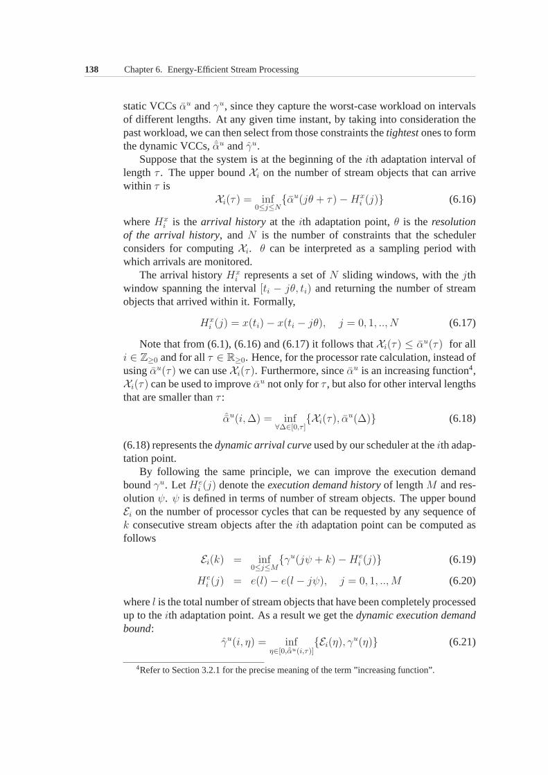
138 Chapter 6. Energy-Efficient Stream Processing
static VCCsαu andγu, since they capture the worst-case workload on intervalsof different lengths. At any given time instant, by taking into consideration thepast workload, we can then select from those constraints thetightestones to formthe dynamic VCCs,αu andγu.
Suppose that the system is at the beginning of theith adaptation interval oflengthτ . The upper boundXi on the number of stream objects that can arrivewithin τ is
Xi(τ) = inf0≤j≤N
{αu(jθ + τ) −Hxi (j)} (6.16)
whereHxi is thearrival history at theith adaptation point,θ is the resolution
of the arrival history, andN is the number of constraints that the schedulerconsiders for computingXi. θ can be interpreted as a sampling period withwhich arrivals are monitored.
The arrival historyHxi represents a set ofN sliding windows, with thejth
window spanning the interval[ti − jθ, ti) and returning the number of streamobjects that arrived within it. Formally,
Hxi (j) = x(ti) − x(ti − jθ), j = 0, 1, .., N (6.17)
Note that from (6.1), (6.16) and (6.17) it follows thatXi(τ) ≤ αu(τ) for alli ∈ Z≥0 and for allτ ∈ R≥0. Hence, for the processor rate calculation, instead ofusingαu(τ) we can useXi(τ). Furthermore, sinceαu is an increasing function4,Xi(τ) can be used to improveαu not only forτ , but also for other interval lengthsthat are smaller thanτ :
ˆαu(i,∆) = inf∀∆∈[0,τ ]
{Xi(τ), αu(∆)} (6.18)
(6.18) represents thedynamic arrival curveused by our scheduler at theith adap-tation point.
By following the same principle, we can improve the executiondemandboundγu. LetHe
i (j) denote theexecution demand historyof lengthM and res-olutionψ. ψ is defined in terms of number of stream objects. The upper boundEi on the number of processor cycles that can be requested by anysequence ofk consecutive stream objects after theith adaptation point can be computed asfollows
Ei(k) = inf0≤j≤M
{γu(jψ + k) −Hei (j)} (6.19)
Hei (j) = e(l) − e(l − jψ), j = 0, 1, ..,M (6.20)
wherel is the total number of stream objects that have been completely processedup to theith adaptation point. As a result we get thedynamic execution demandbound:
γu(i, η) = infη∈[0, ˆαu(i,τ)]
{Ei(η), γu(η)} (6.21)
4Refer to Section 3.2.1 for the precise meaning of the term ”increasing function”.
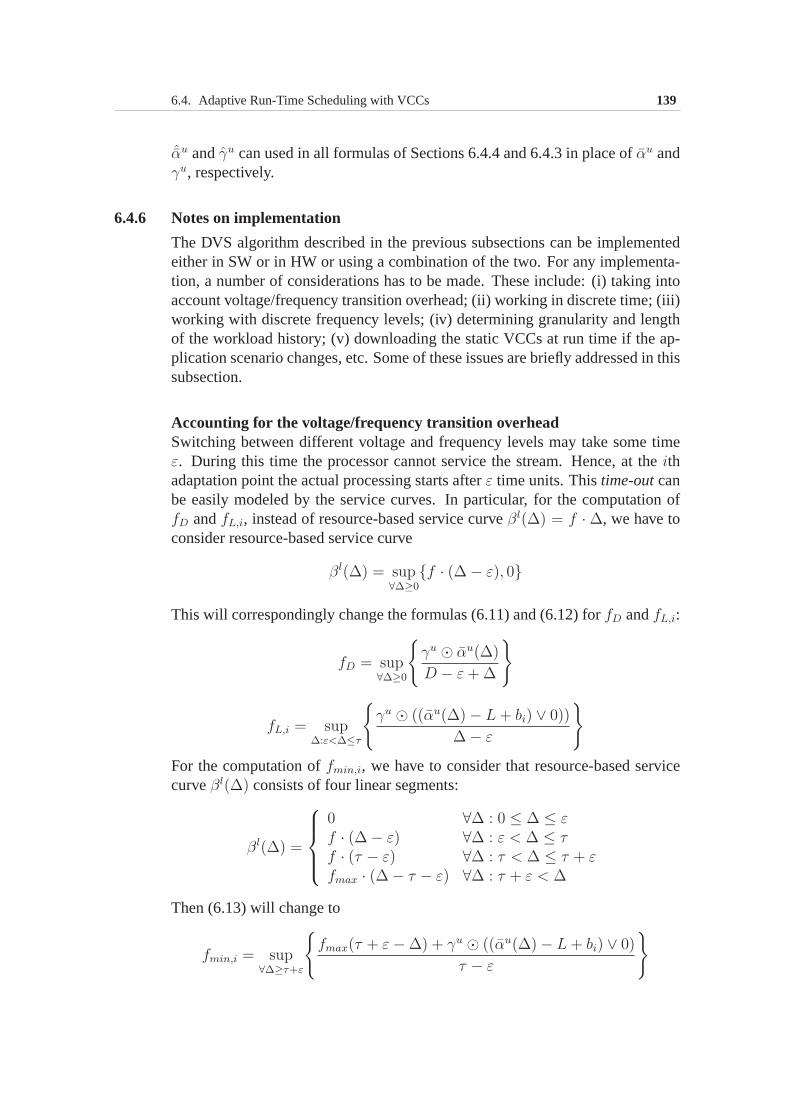
6.4. Adaptive Run-Time Scheduling with VCCs 139
ˆαu andγu can used in all formulas of Sections 6.4.4 and 6.4.3 in place of αu andγu, respectively.
6.4.6 Notes on implementation
The DVS algorithm described in the previous subsections canbe implementedeither in SW or in HW or using a combination of the two. For any implementa-tion, a number of considerations has to be made. These include: (i) taking intoaccount voltage/frequency transition overhead; (ii) working in discrete time; (iii)working with discrete frequency levels; (iv) determining granularity and lengthof the workload history; (v) downloading the static VCCs at runtime if the ap-plication scenario changes, etc. Some of these issues are briefly addressed in thissubsection.
Accounting for the voltage/frequency transition overheadSwitching between different voltage and frequency levels may take some timeε. During this time the processor cannot service the stream. Hence, at theithadaptation point the actual processing starts afterε time units. Thistime-outcanbe easily modeled by the service curves. In particular, for the computation offD andfL,i, instead of resource-based service curveβl(∆) = f · ∆, we have toconsider resource-based service curve
βl(∆) = sup∀∆≥0
{f · (∆ − ε), 0}
This will correspondingly change the formulas (6.11) and (6.12) forfD andfL,i:
fD = sup∀∆≥0
{
γu ⊙ αu(∆)
D − ε+ ∆
}
fL,i = sup∆:ε<∆≤τ
{
γu ⊙ ((αu(∆) − L+ bi) ∨ 0))
∆ − ε
}
For the computation offmin,i, we have to consider that resource-based servicecurveβl(∆) consists of four linear segments:
βl(∆) =
0 ∀∆ : 0 ≤ ∆ ≤ εf · (∆ − ε) ∀∆ : ε < ∆ ≤ τf · (τ − ε) ∀∆ : τ < ∆ ≤ τ + εfmax · (∆ − τ − ε) ∀∆ : τ + ε < ∆
Then (6.13) will change to
fmin,i = sup∀∆≥τ+ε
{
fmax(τ + ε− ∆) + γu ⊙ ((αu(∆) − L+ bi) ∨ 0)
τ − ε
}
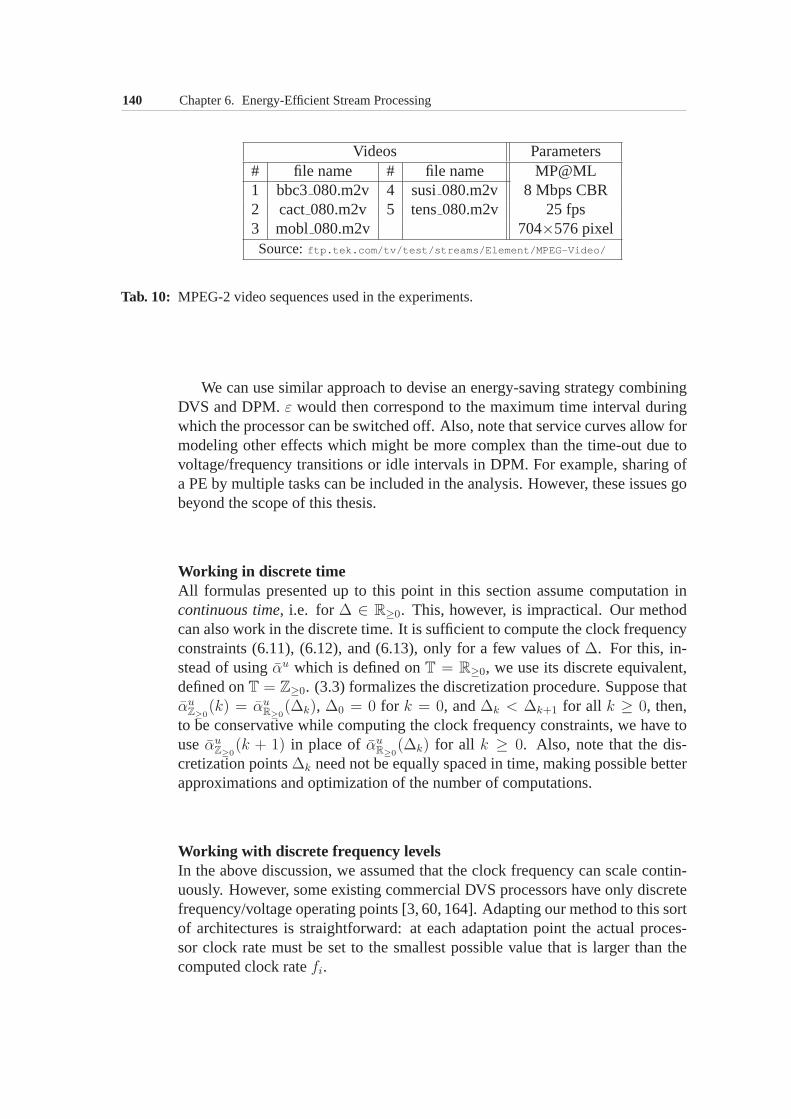
140 Chapter 6. Energy-Efficient Stream Processing
Videos Parameters# file name # file name MP@ML1 bbc3080.m2v 4 susi080.m2v 8 Mbps CBR2 cact080.m2v 5 tens080.m2v 25 fps3 mobl 080.m2v 704×576 pixelSource:ftp.tek.com/tv/test/streams/Element/MPEG-Video/
Tab. 10: MPEG-2 video sequences used in the experiments.
We can use similar approach to devise an energy-saving strategy combiningDVS and DPM.ε would then correspond to the maximum time interval duringwhich the processor can be switched off. Also, note that service curves allow formodeling other effects which might be more complex than the time-out due tovoltage/frequency transitions or idle intervals in DPM. For example, sharing ofa PE by multiple tasks can be included in the analysis. However, these issues gobeyond the scope of this thesis.
Working in discrete timeAll formulas presented up to this point in this section assume computation incontinuous time, i.e. for ∆ ∈ R≥0. This, however, is impractical. Our methodcan also work in the discrete time. It is sufficient to computethe clock frequencyconstraints (6.11), (6.12), and (6.13), only for a few values of ∆. For this, in-stead of usingαu which is defined onT = R≥0, we use its discrete equivalent,defined onT = Z≥0. (3.3) formalizes the discretization procedure. Suppose thatαu
Z≥0(k) = αu
R≥0(∆k), ∆0 = 0 for k = 0, and∆k < ∆k+1 for all k ≥ 0, then,
to be conservative while computing the clock frequency constraints, we have touseαu
Z≥0(k + 1) in place ofαu
R≥0(∆k) for all k ≥ 0. Also, note that the dis-
cretization points∆k need not be equally spaced in time, making possible betterapproximations and optimization of the number of computations.
Working with discrete frequency levelsIn the above discussion, we assumed that the clock frequencycan scale contin-uously. However, some existing commercial DVS processors have only discretefrequency/voltage operating points [3, 60, 164]. Adaptingour method to this sortof architectures is straightforward: at each adaptation point the actual proces-sor clock rate must be set to the smallest possible value thatis larger than thecomputed clock ratefi.
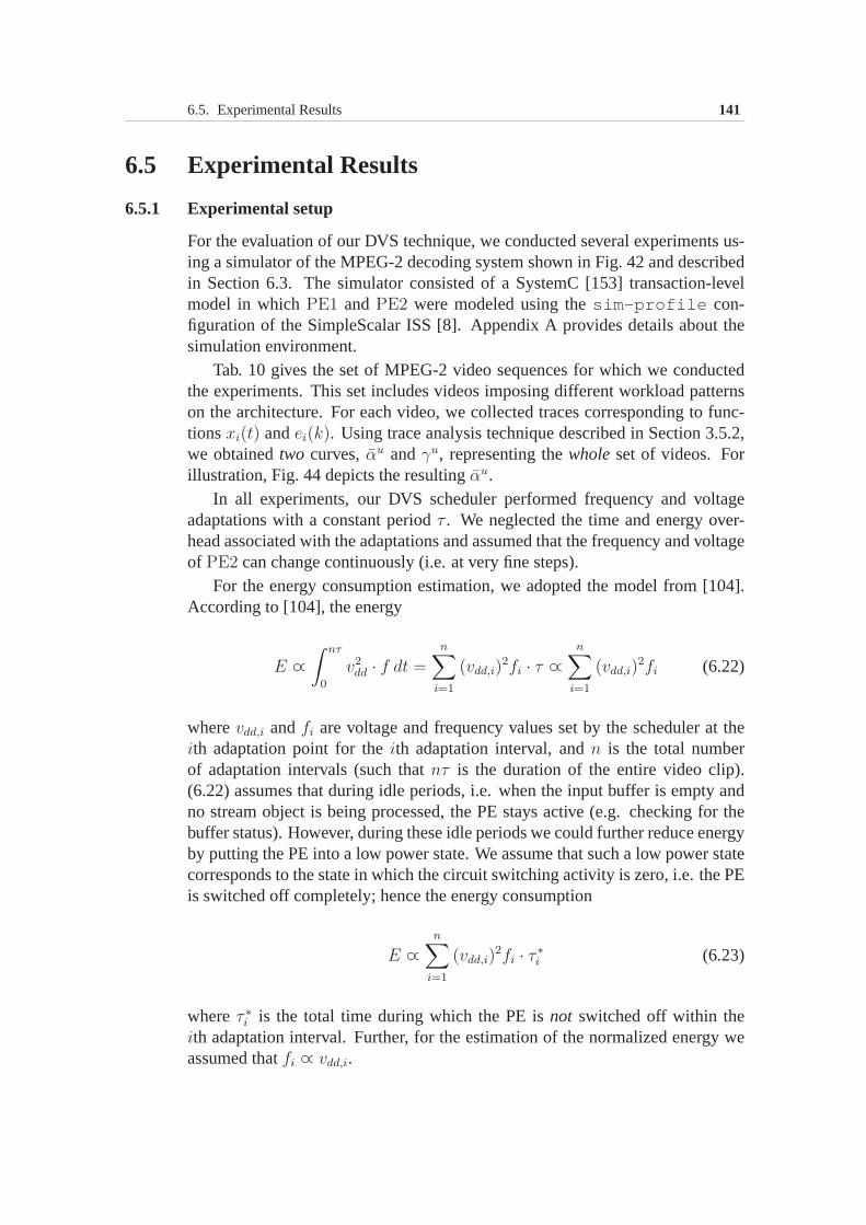
6.5. Experimental Results 141
6.5 Experimental Results
6.5.1 Experimental setup
For the evaluation of our DVS technique, we conducted several experiments us-ing a simulator of the MPEG-2 decoding system shown in Fig. 42and describedin Section 6.3. The simulator consisted of a SystemC [153] transaction-levelmodel in whichPE1 andPE2 were modeled using thesim-profile con-figuration of the SimpleScalar ISS [8]. Appendix A provides details about thesimulation environment.
Tab. 10 gives the set of MPEG-2 video sequences for which we conductedthe experiments. This set includes videos imposing different workload patternson the architecture. For each video, we collected traces corresponding to func-tionsxi(t) andei(k). Using trace analysis technique described in Section 3.5.2,we obtainedtwo curves,αu andγu, representing thewholeset of videos. Forillustration, Fig. 44 depicts the resultingαu.
In all experiments, our DVS scheduler performed frequency and voltageadaptations with a constant periodτ . We neglected the time and energy over-head associated with the adaptations and assumed that the frequency and voltageof PE2 can change continuously (i.e. at very fine steps).
For the energy consumption estimation, we adopted the modelfrom [104].According to [104], the energy
E ∝
∫ nτ
0
v2dd · f dt =
n∑
i=1
(vdd,i)2fi · τ ∝
n∑
i=1
(vdd,i)2fi (6.22)
wherevdd,i andfi are voltage and frequency values set by the scheduler at theith adaptation point for theith adaptation interval, andn is the total numberof adaptation intervals (such thatnτ is the duration of the entire video clip).(6.22) assumes that during idle periods, i.e. when the inputbuffer is empty andno stream object is being processed, the PE stays active (e.g. checking for thebuffer status). However, during these idle periods we couldfurther reduce energyby putting the PE into a low power state. We assume that such a low power statecorresponds to the state in which the circuit switching activity is zero, i.e. the PEis switched off completely; hence the energy consumption
E ∝
n∑
i=1
(vdd,i)2fi · τ ∗i (6.23)
whereτ ∗i is the total time during which the PE isnot switched off within theith adaptation interval. Further, for the estimation of the normalized energy weassumed thatfi ∝ vdd,i.
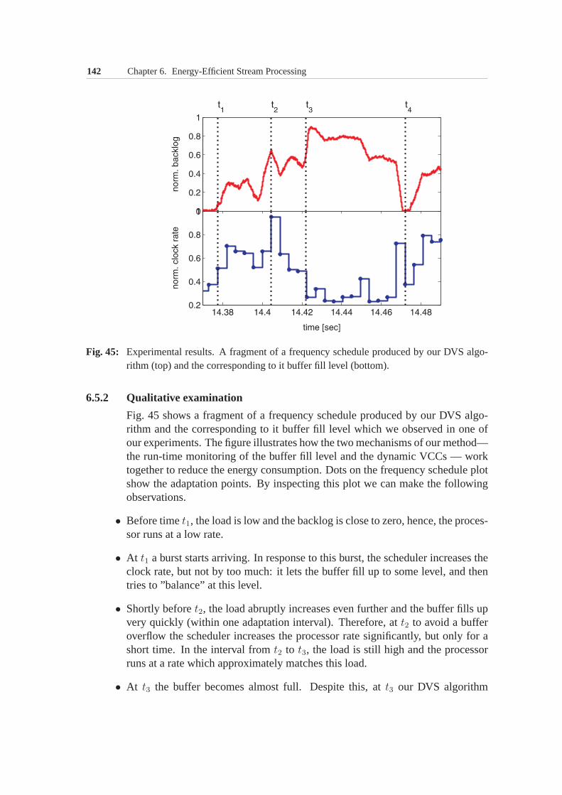
142 Chapter 6. Energy-Efficient Stream Processing
Fig. 45: Experimental results. A fragment of a frequency schedule produced by our DVS algo-rithm (top) and the corresponding to it buffer fill level (bottom).
6.5.2 Qualitative examination
Fig. 45 shows a fragment of a frequency schedule produced by our DVS algo-rithm and the corresponding to it buffer fill level which we observed in one ofour experiments. The figure illustrates how the two mechanisms of our method—the run-time monitoring of the buffer fill level and the dynamic VCCs — worktogether to reduce the energy consumption. Dots on the frequency schedule plotshow the adaptation points. By inspecting this plot we can make the followingobservations.
• Before timet1, the load is low and the backlog is close to zero, hence, the proces-sor runs at a low rate.
• At t1 a burst starts arriving. In response to this burst, the scheduler increases theclock rate, but not by too much: it lets the buffer fill up to some level, and thentries to ”balance” at this level.
• Shortly beforet2, the load abruptly increases even further and the buffer fills upvery quickly (within one adaptation interval). Therefore,at t2 to avoid a bufferoverflow the scheduler increases the processor rate significantly, but only for ashort time. In the interval fromt2 to t3, the load is still high and the processorruns at a rate which approximately matches this load.
• At t3 the buffer becomes almost full. Despite this, att3 our DVS algorithm
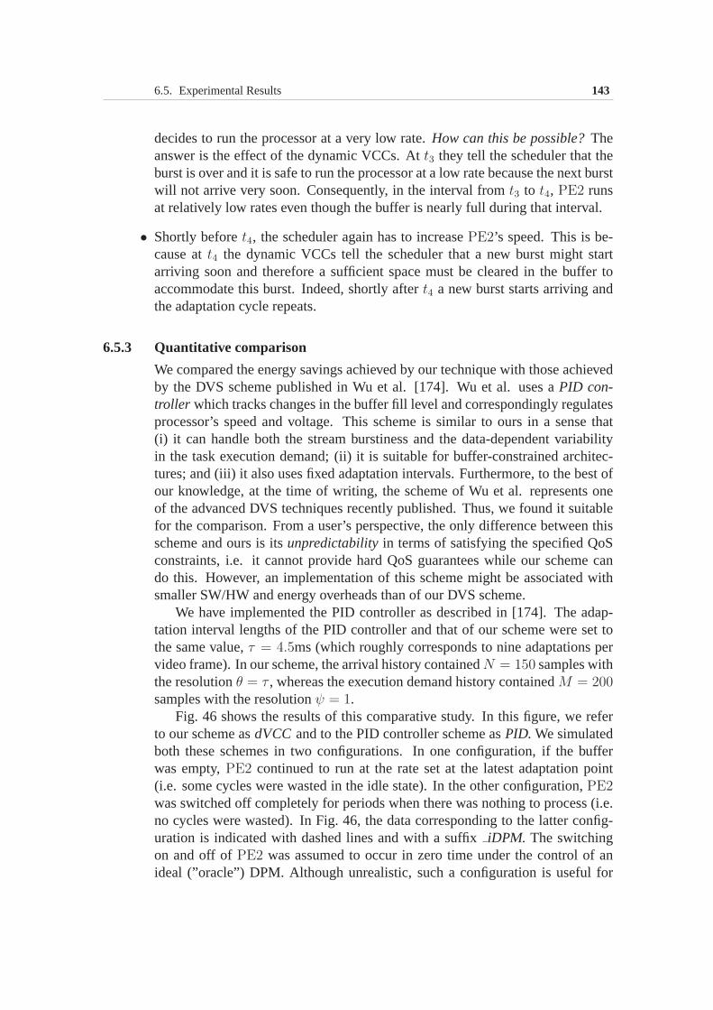
6.5. Experimental Results 143
decides to run the processor at a very low rate.How can this be possible?Theanswer is the effect of the dynamic VCCs. Att3 they tell the scheduler that theburst is over and it is safe to run the processor at a low rate because the next burstwill not arrive very soon. Consequently, in the interval fromt3 to t4, PE2 runsat relatively low rates even though the buffer is nearly fullduring that interval.
• Shortly beforet4, the scheduler again has to increasePE2’s speed. This is be-cause att4 the dynamic VCCs tell the scheduler that a new burst might startarriving soon and therefore a sufficient space must be cleared in the buffer toaccommodate this burst. Indeed, shortly aftert4 a new burst starts arriving andthe adaptation cycle repeats.
6.5.3 Quantitative comparison
We compared the energy savings achieved by our technique with those achievedby the DVS scheme published in Wu et al. [174]. Wu et al. uses aPID con-troller which tracks changes in the buffer fill level and correspondingly regulatesprocessor’s speed and voltage. This scheme is similar to ours in a sense that(i) it can handle both the stream burstiness and the data-dependent variabilityin the task execution demand; (ii) it is suitable for buffer-constrained architec-tures; and (iii) it also uses fixed adaptation intervals. Furthermore, to the best ofour knowledge, at the time of writing, the scheme of Wu et al. represents oneof the advanced DVS techniques recently published. Thus, wefound it suitablefor the comparison. From a user’s perspective, the only difference between thisscheme and ours is itsunpredictabilityin terms of satisfying the specified QoSconstraints, i.e. it cannot provide hard QoS guarantees while our scheme cando this. However, an implementation of this scheme might be associated withsmaller SW/HW and energy overheads than of our DVS scheme.
We have implemented the PID controller as described in [174]. The adap-tation interval lengths of the PID controller and that of ourscheme were set tothe same value,τ = 4.5ms (which roughly corresponds to nine adaptations pervideo frame). In our scheme, the arrival history containedN = 150 samples withthe resolutionθ = τ , whereas the execution demand history containedM = 200samples with the resolutionψ = 1.
Fig. 46 shows the results of this comparative study. In this figure, we referto our scheme asdVCC and to the PID controller scheme asPID. We simulatedboth these schemes in two configurations. In one configuration, if the bufferwas empty,PE2 continued to run at the rate set at the latest adaptation point(i.e. some cycles were wasted in the idle state). In the otherconfiguration,PE2was switched off completely for periods when there was nothing to process (i.e.no cycles were wasted). In Fig. 46, the data corresponding tothe latter config-uration is indicated with dashed lines and with a suffixiDPM. The switchingon and off ofPE2 was assumed to occur in zero time under the control of anideal (”oracle”) DPM. Although unrealistic, such a configuration is useful for
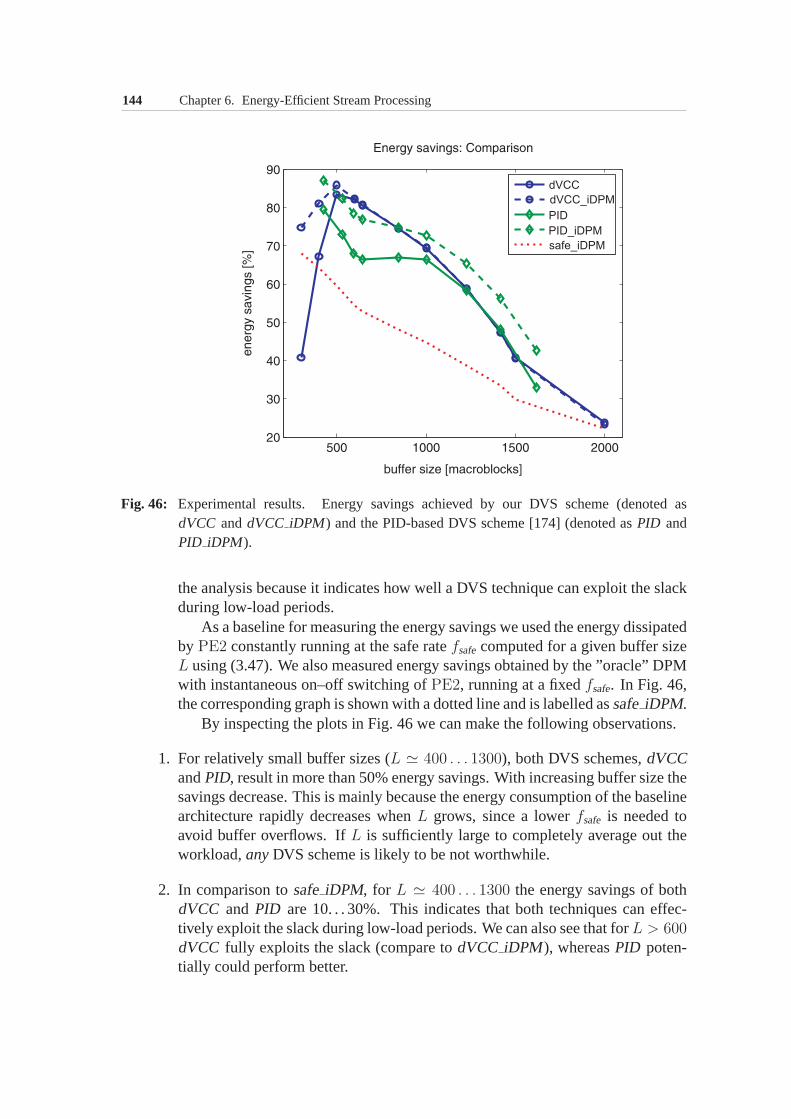
144 Chapter 6. Energy-Efficient Stream Processing
Fig. 46: Experimental results. Energy savings achieved by our DVS scheme (denoted asdVCC anddVCC iDPM ) and the PID-based DVS scheme [174] (denoted asPID andPID iDPM ).
the analysis because it indicates how well a DVS technique can exploit the slackduring low-load periods.
As a baseline for measuring the energy savings we used the energy dissipatedby PE2 constantly running at the safe ratefsafecomputed for a given buffer sizeL using (3.47). We also measured energy savings obtained by the ”oracle” DPMwith instantaneous on–off switching ofPE2, running at a fixedfsafe. In Fig. 46,the corresponding graph is shown with a dotted line and is labelled assafeiDPM.
By inspecting the plots in Fig. 46 we can make the following observations.
1. For relatively small buffer sizes (L ≃ 400 . . . 1300), both DVS schemes,dVCCandPID, result in more than 50% energy savings. With increasing buffer size thesavings decrease. This is mainly because the energy consumption of the baselinearchitecture rapidly decreases whenL grows, since a lowerfsafe is needed toavoid buffer overflows. IfL is sufficiently large to completely average out theworkload,anyDVS scheme is likely to be not worthwhile.
2. In comparison tosafeiDPM, for L ≃ 400 . . . 1300 the energy savings of bothdVCC andPID are 10. . . 30%. This indicates that both techniques can effec-tively exploit the slack during low-load periods. We can also see that forL > 600dVCC fully exploits the slack (compare todVCC iDPM ), whereasPID poten-tially could perform better.
6.5. Experimental Results 145
Fig. 47: Experimental results. Energy savings vs. adaptation interval length, fordifferent buffersizesL.
3. ForL > 450 energy savings fromdVCC are at least as high as fromPID, whilefor L < 450 PID saves 15% more energy thandVCC. This is the price forthe hard QoS guarantees provided bydVCC. If the user specifiesL as the bufferconstraint,dVCC guarantees that the maximum buffer fill level will never exceedL. In contrast,PID cannot guarantee this. InPID the user can only specify atarget, not themaximum, buffer fill level. The PID controller will then try tokeep the backlog at this level. Bursty workloads and stringent buffer constraintsrequire the PID controller to quickly respond to workload changes. This leads to(large) oscillations around the target level during adaptations, which means thatif the target level has been set improperly a buffer overflow may occur. As anexample, the left most point in thePID graph was obtained by setting the targetbuffer fill level to 20 macroblocks, while the maximum backlog registered in thebuffer for this setting was about 450 macroblocks. This problem withPID mightbe less acute for smoother workloads and larger buffers.
6.5.4 Energy savings vs. implementation overhead
The estimated computational requirement of our DVS algorithm, for parame-ters (τ,N, ψ,M) set as described above, (i.e.τ = 4.5ms,N = 150, ψ = 1,M = 200), is about 0.5 MIPS. This overhead scales linearly with the values ofthese parameters. It is also relatively low in comparison tothe average workloadimposed onPE2 by a DVD-quality video stream (about 45 MIPS in our setup).
146 Chapter 6. Energy-Efficient Stream Processing
Fig. 47 shows measured tradeoff plots between the adaptation interval lengthτ and the energy savings obtained by our scheme for different buffer sizesL.In Fig. 47, we can see that smaller adaptation intervals leadto higher energysavings. Achieving the energy reduction for smaller buffersizes comparable tothat achieved for larger buffer sizes necessitates more frequent adaptations andtherefore results in higher run-time overhead. This is again the price for theguaranteed QoS.
6.6 SummaryIn this chapter, we described a new DVS scheduling scheme specifically tar-geted towards processing media streams on architectures with restricted buffersizes. In contrast to previously proposed DVS schemes, our scheme provideshard QoS guarantees and accounts for both, the variability of the task execu-tion demand and the burstiness of processed streams. Our experiments showedthat the scheme achieves energy savings comparable to thoseobtained by pre-vious approaches. The advantages of our scheme can be attributed to the novelcombination of the off-line worst-case workload characterization based on VCCswith the run-time improvement of the worst-case bounds. Theimplementationand run-time overhead of our scheme, although modest, mightbe slightly higherthan that of previous schemes. However, this is the price that has to be paid forpredictability of the system, i.e. for its ability to provide hard QoS guarantees.
7Conclusions
In this thesis, we have addressed the problem of workload modeling for system-level design of heterogeneous multiprocessor embedded computers whose mainfunctionality involves real-time processing of media streams. The complex, vari-able nature of the multimedia workloads imposed on these computers greatlycomplicates their system-level design. The central resultof this thesis is awork-load modelthat helps to reduce this design complexity by providing a set of sim-ple but powerful abstractions to accurately capture the variability characteristicsof the multimedia workloads. We have formally defined this workload model,demonstrated its advantages over existing workload characterization methodsand showed some of its applications in the system-level design of heterogeneousmultiprocessor system-on-chip (MpSoC) architectures. In particular, we wouldlike to point out the following main outcomes of this work:
• We have introduced the concept ofVariability Characterization Curves(VCCs)—a generic model for the worst- and best-case variability characterization of en-tire classes of increasing functions and sequences — and based on this conceptdefined our model for the multimedia workload characterization (multimediaVCCs).
• We have used our workload model to enhance modeling capabilities of theMod-ular Performance Analysis[159, 160] framework based onReal-Time Calculus[24, 121, 157, 158]. This has resulted in the definition of newmodeling con-structs, calledworkload transformations, which have enabled an accurate andefficient performance analysis of heterogeneous multiprocessor embedded sys-tems under variable multimedia workloads. Our experimental results showedthat the workload transformations allow to obtain significantly tighter perfor-
148 Chapter 7. Conclusions
mance bounds than those achievable without using our workload model.
• We have demonstrated application of our workload model in design of resourcemanagement policies for multimedia MpSoCs. Our workload model permits toformulate and address a class of scheduling problems which has not been ad-dressed before:stream scheduling on buffer-constrained architectures with hardQoS guarantees. We have proposed a design framework for efficient explorationand optimization of this class of schedulers and showed its utility using casestudies involving TDMA scheduling disciplines.
• Based on our workload model we have developed arun-time processor rateadaptation strategywhich can be used in conjunction with the dynamic volt-age scaling for energy-efficient media stream processing onbuffer-constrainedarchitectures. In comparison to other methods addressing similar problems,our scheme can handle multimedia workloads characterized by both, the data-dependent variability in the task execution timeand the burstiness in the on-chiptraffic arising out of multimedia processing; and at the sametime it can providehard QoS guarantees. An experimental evaluation showed that our scheme canachieve considerable energy savings, comparable to those obtainable with an-other state-of-the-art DVS scheme (which is, however, unable to provide hardQoS guarantees).
• Finally, we have demonstrated how our workload model can be used to de-sign representative workload scenariosfor simulation-based system-level per-formance evaluation of multimedia MpSoCs. We have proposed amethod for(automatic) classification of media streams based on the variability characteris-tics of the workload they may impose on the architecture. We are not aware ofany other method addressing this important issue in the system-level design ofMpSoCs.
ASimulation Framework
This chapter describes the simulation framework which was used in experimen-tal case studies presented throughout this thesis.
Fig. 48 shows an overview of the simulation framework and itsrelations withthe methods developed in this thesis. Two major components of the simulationframework are
• an instruction set simulator(ISS) and
• asystem simulator.
ISS is used to collect information about behavior of application tasks mapped forexecution on to programmable processing elements of a target MpSoC architec-ture. This information is collected and stored in the form oftraces. These tracesare then used in two different ways. First, we can compute from them VCCs,which are needed by the VCC-based methods presented in this thesis. Second,the traces serve as an input to the system simulator to simulate execution of theapplication on the target MpSoC architecture.
The system simulator allows to measure various performanceindexes of agiven application-to-architecture mapping (system configuration). These mea-surements can then be compared with corresponding numbers obtained frommathematical performance models.
The following two sections give details on ISS and the systemsimulator.
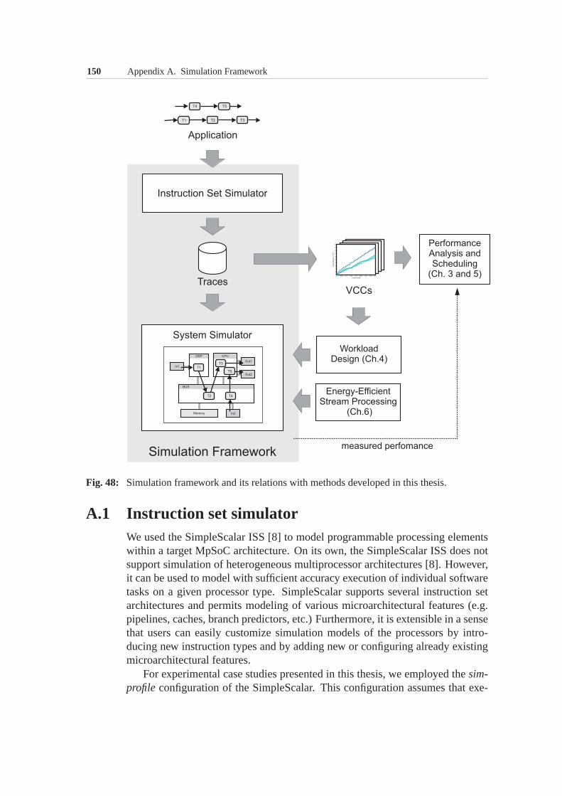
150 Appendix A. Simulation Framework
Fig. 48: Simulation framework and its relations with methods developed in this thesis.
A.1 Instruction set simulatorWe used the SimpleScalar ISS [8] to model programmable processing elementswithin a target MpSoC architecture. On its own, the SimpleScalar ISS does notsupport simulation of heterogeneous multiprocessor architectures [8]. However,it can be used to model with sufficient accuracy execution of individual softwaretasks on a given processor type. SimpleScalar supports several instruction setarchitectures and permits modeling of various microarchitectural features (e.g.pipelines, caches, branch predictors, etc.) Furthermore,it is extensible in a sensethat users can easily customize simulation models of the processors by intro-ducing new instruction types and by adding new or configuringalready existingmicroarchitectural features.
For experimental case studies presented in this thesis, we employed thesim-profile configuration of the SimpleScalar. This configuration assumes that exe-
A.2. System simulator 151
cution of every instruction in a program code takes exactly one processor cycle,i.e. it does not account for possible stalls due to, for example, pipeline hazardsor cache misses. Although thesim-profileconfiguration might be too inaccuratefor the microarchitecture design, for the system level at which we considered theMpSoC architectures, it represents an appropriate choice.
For modeling processing elements we used an instruction setsimilar to thatused in MIPS3000 processors, but without floating point support. This instruc-tion set had application-specific extensions for video decoding, e.g. instructionsfor bitstream access, IDCT computation and special block-based memory ad-dressing modes. To collect useful information about the data-dependent behav-ior of application tasks, we had to augment the SimpleScalarwith logging andtrace collection facilities.
A.2 System simulatorOur simulation framework allows to easily construct a simulation model of agiven application-to-architecture mapping. We refer to such a simulation modelas the system simulator. The system simulator represents atransaction-levelmodel [34] of the system in which implementation details of individual hard-ware components and application tasks are abstracted away.Instead, the hard-ware architecture is represented by a set of (coarse-grain)computation and com-munication resources with certain processing capabilities, while the applicationtasks are modeled as clients requesting these resources (i.e. generating demandsfor these resources). At this level of abstraction, there isno principle differencebetween computation and communication resources (or tasks).
An application is represented by a set of concurrent tasks communicating viaunidirectional FIFO channels. The execution model is the same as the one de-scribed in Section 3.3.1 besides the fact that the FIFO channels have finite sizesand block write operations whenever they are full. The finitechannel sizes allowto model the buffer space constraints resulting from mapping of the applicationonto the hardware architecture. A write operation into a FIFO channel is re-garded as a transaction. A task may accomplish several such transactions duringits execution.
When a task is activated it generates a request for the resource onto which itis mapped. In the current implementation, the amount of resources requested iseither fixed to a constant value or obtained from the traces collected using the ISSdescribed in the previous section. A resource is distributed to tasks in accordancewith the scheduling (or arbitration) policy implemented onthat resource. Theframework supports both preemptive and non-preemptive scheduling policies. Inprinciple, task switching and operating system overheads can be modeled withinthe framework but were not modeled in the experiments presented in this thesis.
The implementation of the system simulator just described fully rests on the

152 Appendix A. Simulation Framework
SystemC C++ library [153] and correspondingly uses of its discrete event simu-lation engine. We have added an abstraction level on top of the SystemC librarywhich allows to quickly construct a new application-to-architecture mapping orto easily change an existing system configuration.
Bibliography
[1] L. Abeni and G. Buttazzo. Resource reservation in dynamic real-timesystems.Real-Time Systems, 27(2):123–167, 2004.
[2] A. Agarwal, C. H. Kim, S. Mukhopadhyay, and K. Roy. Leakage in nano-scale technologies: mechanisms, impact and design considerations. InProceedings of the 41st Annual Conference on Design Automation (DAC),pages 6–11, New York, NY, USA, 2004. ACM Press.
[3] Advanced Micro Devices, Inc. AMD PowerNow! technology.http://www.amd.com, 2005.
[4] A. Andrei, M. Schmitz, P. Eles, Z. Peng, and B. M. Al-Hashimi.Overhead-conscious voltage selection for dynamic and leakage energy re-duction of time-constrained systems. InDesign, Automation and Test inEurope (DATE), page 10518, Washington, DC, USA, 2004. IEEE Com-puter Society.
[5] A. Andrei, M. T. Schmitz, P. Eles, Z. Peng, and B. M. A. Hashimi. Quasi-static voltage scaling for energy minimization with time constraints. InDesign, Automation and Test in Europe (DATE), pages 514–519, Wash-ington, DC, USA, 2005. IEEE Computer Society.
[6] A. Artieri, V. DAlto, R. Chesson, M. Hopkins, and M. C. Rossi. Nomadikopen multimedia platform for next-generation mobile devices. STMicro-electronics Technical Article TA305,http://www.st.com, 2003.
[7] A. Atlas and A. Bestavros. Statistical rate monotonic scheduling. InPro-ceedings of the 19th IEEE Real-Time Systems Symposium (RTSS), page123, Washington, DC, USA, 1998. IEEE Computer Society.
[8] T. Austin, E. Larson, and D. Ernst. SimpleScalar: An infrastructure forcomputer system modeling.IEEE Computer, 35(2):59–67, 2002.
[9] A. Azevedo, I. Issenin, R. Cornea, R. Gupta, N. Dutt, A. Veidenbaum,and A. Nicolau. Profile-based dynamic voltage scheduling using programcheckpoints. InDesign, Automation and Test in Europe (DATE), page168, Washington, DC, USA, 2002. IEEE Computer Society.
154 Bibliography
[10] F. Baccelli, G. Cohen, G. Olsder, and J.-P. Quadrat.Synchronization andLinearity. John Wiley, Sons, New York, 1992.
[11] S. K. Baruah. A general model for recurring real-time tasks. InProceed-ings of the IEEE Real-Time Systems Symposium (RTSS), pages 114–122,1998.
[12] S. K. Baruah. Dynamic- and static-priority scheduling of recurring real-time tasks.Real-Time Systems, 24(1):93–128, 2003.
[13] S. K. Baruah, D. Chen, S. Gorinsky, and A. K. Mok. Generalized multi-frame tasks.Real-Time Systems, 17(1):5–22, 1999.
[14] A. C. Bavier, A. B. Montz, and L. L. Peterson. Predicting MPEG execu-tion times. InSIGMETRICS, pages 131–140, 1998.
[15] L. Benini, D. Bertozzi, D. Bruni, N. Drago, F. Fummi, and M. Pon-cino. SystemC cosimulation and emulation of multiprocessor SoC de-signs.IEEE Computer, 36(4):53–59, 2003.
[16] L. Benini, A. Bogliolo, and G. D. Micheli. A survey of design techniquesfor system-level dynamic power management.IEEE Transactions on VLSISystems, 8(3):299–316, June 2000.
[17] L. Benini and G. D. Micheli. Powering networks on chips: energy-efficient and reliable interconnect design for SoCs. InProceedings of the14th International Symposium on Systems Synthesis (ISSS), pages 33–38,New York, NY, USA, 2001. ACM Press.
[18] S. S. Bhattacharyya, P. K. Murthy, and E. A. Lee. Synthesis of embed-ded software from synchronous dataflow specifications.Journal of VLSISignal Processing Systems, 21(2):151–166, 1999.
[19] G. Bilsen, M. Engels, R. Lauwereins, and J. Peperstraete.Cyclo-staticdataflow.IEEE Transactions on Signal Processing, 44(2):397–408, 1996.
[20] S. Borkar. Design challenges of technology scaling.IEEE Micro,19(4):23–29, 1999.
[21] T. D. Burd and R. W. Brodersen. Energy efficient CMOS microprocessordesign. InHICSS (1), pages 288–297, 1995.
[22] G. C. Buttazzo. Hard Real-time Computing Systems: PredictableScheduling Algorithms And Applications (Real-Time Systems Series).Springer-Verlag Telos, 2004.
[23] S. Chakraborty.System-Level Timing Analysis and Scheduling for Embed-ded Packet Processors. PhD thesis, ETH Zurich, Apr. 2003.
Bibliography 155
[24] S. Chakraborty, S. Kunzli, and L. Thiele. A general framework foranalysing system properties in platform-based embedded system designs.In Design, Automation and Test in Europe (DATE), pages 190–195, Mu-nich, Germany, Mar. 2003. IEEE Press.
[25] S. Chakraborty, S. Kunzli, L. Thiele, A. Herkersdorf, and P. Sagmeister.Performance evaluation of network processor architectures: Combiningsimulation with analytical estimation.Computer Networks, 41(5):641—-665, 2003.
[26] S. Chakraborty and L. Thiele. A new task model for streaming applica-tions and its schedulability analysis. InDesign, Automation and Test inEurope (DATE), pages 486–491, 2005.
[27] A. P. Chandrakasan and R. W. Brodersen.Low Power Digital CMOSDesign. Kluwer Academic Publishers, 1995.
[28] L. H. Chandrasena, P. Chandrasena, and M. J. Liebelt. An energy efficientrate selection algorithm for voltage quantized dynamic voltage scaling. InProceedings of the 14th International Symposium on SystemsSynthesis(ISSS), pages 124–129, New York, NY, USA, 2001. ACM Press.
[29] K. Choi, K. Dantu, W.-C. Cheng, and M. Pedram. Frame-based dynamicvoltage and frequency scaling for a MPEG decoder. InProceedings ofthe 2002 IEEE/ACM International Conference on Computer-AidedDe-sign (ICCAD), pages 732–737, 2002.
[30] K. Choi, R. Soma, and M. Pedram. Off-chip latency-driven dynamic volt-age and frequency scaling for an MPEG decoding. InProceedings of the41st Annual Conference on Design Automation (DAC), pages 544–549,2004.
[31] W. J. Dally and B. Towles. Route packets, not wires: on-chip inteconnec-toin networks. InProceedings of the 38th Conference on Design Automa-tion (DAC), pages 684–689, New York, NY, USA, 2001. ACM Press.
[32] B. P. Dave and N. K. Jha. CASPER: Concurrent hardware-software co-synthesis of hard real-time aperiodic and periodic specifications of em-bedded system architectures. InDesign, Automation and Test in Europe(DATE), pages 118–124, 1998.
[33] B. P. Dave, G. Lakshminarayana, and N. K. Jha. COSYN: Hardware-software co-synthesis of embedded systems. InProceedings of the 34thConference on Design Automation (DAC), pages 703–708, 1997.

156 Bibliography
[34] A. K. Deb, A. Jantsch, and J.Oberg. System design for dsp applications intransaction level modeling paradigm. InProceedings of the 41st AnnualConference on Design Automation (DAC), pages 466–471. ACM Press,2004.
[35] R. P. Dick and N. K. Jha. MOCSYN: Multiobjective core-based single-chip system synthesis. InDesign, Automation and Test in Europe (DATE),pages 263–270, 1999.
[36] K. Diefendorff and P. K. Dubey. How multimedia workloads will changeprocessor design.Computer, 30(9):43–45, 1997.
[37] R. C. Dorf and R. H. Bishop.Modern Control Systems. Addison-WesleyLongman Publishing Co., Inc., Boston, MA, USA, 1994.
[38] S. Dutta, R. Jensen, and A. Rieckmann. Viper: A multiprocessor SOCfor advanced set-top box and digital TV systems.IEEE Design & Test ofComputers, 18(5):21–31, 2001.
[39] L. Eeckhout, H. Vandierendonck, and K. D. Bosschere. Workload de-sign: Selecting representative program-input pairs. InProceedings of the2002 International Conference on Parallel Architectures and CompilationTechniques, pages 83–94. IEEE Computer Society, 2002.
[40] H. El-Rewini, H. H. Ali, and T. G. Lewis. Task scheduling in multi-processing systems.IEEE Computer, 28(12):27–37, 1995.
[41] C. J. Fidge. Real-time schedulability tests for preemptive multitasking.In Selected papers from the 4th Workshop on Parallel and DistributedReal-Time Systems (WPDRTS), pages 61–93, Norwell, MA, USA, 1998.Kluwer Academic Publishers.
[42] K. Flautner, S. Reinhardt, and T. Mudge. Automatic performance settingfor dynamic voltage scaling.Wireless Networks, 8(5):507–520, 2002.
[43] S. Goddard and K. Jeffay. Managing latency and buffer requirements inprocessing graph chains.The Computer Journal, 44(6):486–503, 2001.
[44] K. Goossens, J. Dielissen, J. van Meerbergen, P. Poplavko, A. Radulescu,E. Rijpkema, E. Waterlander, and P. Wielage. Guaranteeing the qualityof services in networks on chip. In A. Jantsch and H. Tenhunen, editors,Networks on Chip, pages 61–82. Kluwer Academic Publishers, Hingham,MA, USA, 2003.
[45] A. D. Gordon.Classification. Chapman & Hall/CRC, 1999.
Bibliography 157
[46] K. Govil, E. Chan, and H. Wasserman. Comparing algorithmsfor dynamicspeed-setting of a low-power CPU. InProceedings of the 1st Annual In-tern. Conf. on Mobile Computing and Networking, pages 13–25. ACMPress, 1995.
[47] F. Gruian and K. Kuchcinski. LEneS: task scheduling forlow-energysystems using variable supply voltage processors. InProceedings of the2001 Conference on Asia South Pacific Design Automation (ASP-DAC),pages 449–455, 2001.
[48] J. C. P. Gutierrez and M. G. Harbour. Offset-based response time analysisof distributed systems scheduled under EDF. InProceedings of the 15thEuromicro Conference on Real-Time Systems (ECRTS), pages 3–12, 2003.
[49] V. Gutnik and A. P. Chandrakasan. Embedded power supply for low-power DSP.IEEE Transactions on VLSI Systems, 5(4):425–435, 1997.
[50] S. Ha and E. A. Lee. Compile-time scheduling of dynamic constructs indataflow program graphs.IEEE Transactions on Computers, 46(7):768–778, 1997.
[51] A. Hamann and R. Ernst. TDMA time slot and turn optimization withevolutionary search techniques. InDesign, Automation and Test in Europe(DATE), pages 312–317, Washington, DC, USA, 2005. IEEE ComputerSociety.
[52] F. Harmsze, A. H. Timmer, and J. L. van Meerbergen. Memory arbitrationand cache management in stream-based systems. InDesign, Automationand Test in Europe (DATE), pages 257–262, 2000.
[53] J. Helmig. Developing core software technologies for TI’s OMAP plat-form. Texas Instruments,http://www.ti.com, 2002.
[54] I. Hong, D. Kirovski, G. Qu, M. Potkonjak, and M. B. Srivastava. Poweroptimization of variable voltage core-based systems. InProceedings ofthe 35th Annual Conference on Design Automation (DAC), pages 176–181, New York, NY, USA, 1998. ACM Press.
[55] I. Hong, M. Potkonjak, and M. B. Srivastava. On-line scheduling ofhard real-time tasks on variable voltage processor. InProceedings ofthe 1998 IEEE/ACM International Conference on Computer-AidedDe-sign (ICCAD), pages 653–656, New York, NY, USA, 1998. ACM Press.
[56] S. Hua, G. Qu, and S. S. Bhattacharyya. Energy reduction techniques formultimedia applications with tolerance to deadline misses. In Proceed-ings of the 40th Conference on Design Automation (DAC), pages 131–136,New York, NY, USA, 2003. ACM Press.

158 Bibliography
[57] C. J. Hughes, P. Kaul, S. V. Adve, R. Jain, C. Park, and J. Srinivasan.Variability in the execution of multimedia applications and implicationsfor architecture. InProceedings of the 28th Annual International Sympo-sium on Computer Architecture, pages 254–265. ACM Press, 2001.
[58] IBM PowerPC.http://www.chips.ibm.com/products/powerpc/,2005.
[59] C. Im, S. Ha, and H. Kim. Dynamic voltage scheduling with buffers inlow-power multimedia applications.Transactions on Embedded Comput-ing Systems, 3(4):686–705, 2004.
[60] Intel Corporation, Enhanced Intel SpeedStep technology.http://www.intel.com, 2005.
[61] T. Ishihara and H. Yasuura. Voltage scheduling problemfor dynamicallyvariable voltage processors. InProceedings of the 1998 InternationalSymposium on Low Power Electronics and Design (ISLPED), pages 197–202, New York, NY, USA, 1998. ACM Press.
[62] S. Ishiwata, T. Yamakage, Y. Tsuboi, T. Shimazawa, T. Kitazawa,S. Michinaka, K. Yahagi, H. Takeda, A. Oue, T. Kodama, N. Matsumoto,T. Kamei, M. Saito, T. Miyamori, G. Ootomo, and M. Matsui. A single-chip MPEG-2 codec based on customizable media embedded processor.IEEE Journal of Solid-State Circuits, 38(3):530–540, 2003.
[63] H. Iwasaki, J. Naganuma, K. Nitta, K. Nakamura, T. Yoshitome,M. Ogura, Y. Nakajima, Y. Tashiro, T. Onishi, M. Ikeda, and M.Endo.Single-chip MPEG-2 422P@HL CODEC LSI with multi-chip configura-tion for large scale processing beyond HDTV level. InDesign, Automationand Test in Europe (DATE), pages 20002–20007, 2003.
[64] A. Iyer and D. Marculescu. Power and performance evaluation of globallyasynchronous locally synchronous processors. InProceedings of the 29thAnnual International Symposium on Computer Architecture (ISCA), pages158–168, Washington, DC, USA, 2002. IEEE Computer Society.
[65] K. Jeffay and S. Goddard. A theory of rate-based execution. In Pro-ceedings of the 20th IEEE Real-Time Systems Symposium (RTSS), pages304–314, 1999.
[66] R. Jejurikar, C. Pereira, and R. Gupta. Leakage aware dynamic volt-age scaling for real-time embedded systems. InProceedings of the 41stAnnual Conference on Design Automation (DAC), pages 275–280, NewYork, NY, USA, 2004. ACM Press.
Bibliography 159
[67] M. Jersak and R. Ernst. Enabling scheduling analysis of heterogeneoussystems with multi-rate data dependencies and rate intervals. In Proceed-ings of the 40th conference on Design automation (DAC), pages 454–459,New York, NY, USA, 2003. ACM Press.
[68] M. Jersak, K. Richter, and R. Ernst. Performance analysisfor complexembedded applications.International Journal of Embedded Systems, Spe-cial Issue on Codesign for SoC, 2004.
[69] N. K. Jha. Low power system scheduling and synthesis. InProceedingsof the 2001 IEEE/ACM International Conference on Computer-Aided De-sign (ICCAD), pages 259–263, Piscataway, NJ, USA, 2001. IEEE Press.
[70] G. Kahn. The semantics of simple language for parallel programming. InIFIP Congress, pages 471–475, 1974.
[71] A. Kalavade and P. Moghe. A tool for performance estimation of net-worked embedded end-systems. InProceedings of the 35th Conferenceon Design Automation Conference (DAC), pages 257–262. ACM/IEEE,June 1998.
[72] K. Keutzer, S. Malik, A. R. Newton, J. M. Rabaey, and A. Sangiovanni-Vincentelli. System-level design: Orthogonalization of concerns andplatform-based design.IEEE Transactions on Computer-Aided Design,19(12), 2000.
[73] C. Kim and K. Roy. Dynamic Vth scaling scheme for active leakage powerreduction. InDesign, Automation and Test in Europe (DATE), page 163,Washington, DC, USA, 2002. IEEE Computer Society.
[74] S. Kim, C. Im, and S. Ha. Schedule-aware performance estimation ofcommunication architecture for efficient design space exploration. InPro-ceedings of the 1st IEEE/ACM/IFIP International Conference on Hard-ware/Software Codesign and System Synthesis (CODES+ISSS), pages195–200, New York, NY, USA, 2003. ACM Press.
[75] S. Kim, C. Im, and S. Ha. Efficient exploration of on-chip bus architec-tures and memory allocation. InProceedings of the 2nd IEEE/ACM/IFIPInternational Conference on Hardware/Software Codesign and SystemSynthesis (CODES+ISSS), pages 248–253, New York, NY, USA, 2004.ACM Press.
[76] H. Kopetz.Real-time Systems: Design Principles for Distributed Embed-ded Applications. Boston Kluwer Academic Publishers, 1997.
[77] C. E. Kozyrakis and D. A. Patterson. A new direction for computer archi-tecture research.Computer, 31(11):24–32, 1998.
160 Bibliography
[78] M. Krunz and S. K. Tripathi. On the characterization of VBR MPEGstreams.SIGMETRICS Perform. Eval. Rev., 25(1):192–202, 1997.
[79] S. Kumar. On packet switched networks for on-chip communication. InA. Jantsch and H. Tenhunen, editors,Networks on Chip, pages 85–106.Kluwer Academic Publishers, Hingham, MA, USA, 2003.
[80] Y.-K. Kwok and I. Ahmad. Static scheduling algorithms for allocat-ing directed task graphs to multiprocessors.ACM Computing Surveys,31(4):406–471, 1999.
[81] W.-C. Kwon and T. Kim. Optimal voltage allocation techniques for dy-namically variable voltage processors.Transactions on Embedded Com-puting Systems, 4(1):211–230, 2005.
[82] T. Lafage and A. Seznec. Choosing representative slicesof program exe-cution for microarchitecture simulations: a preliminary application to thedata stream. InWorkload characterization of emerging computer applica-tions, pages 145–163. Kluwer Academic Publishers, 2001.
[83] K. Lahiri, A. Raghunathan, and S. Dey. System level performance analy-sis for designing on-chip communication architectures.IEEE Trans-actions on Computer Aided-Design of Integrated Circuits and Systems,20(6):768–783, 2001.
[84] A. A. Lazar, G. Pacifici, and D. E. Pendarakis. Modeling video sourcesfor real-time scheduling.Multimedia Systems, 1(6):253–266, 1994.
[85] J.-Y. Le Boudec and P. Thiran.Network calculus: a theory of deterministicqueuing systems for the Internet. Springer-Verlag New York, Inc., 2001.
[86] C. Lee, M. Potkonjak, and W. H. Mangione-Smith. MediaBench: a toolfor evaluating and synthesizing multimedia and communicatons systems.In Proceedings of the 30th annual ACM/IEEE International Symposiumon Microarchitecture, pages 330–335. IEEE Computer Society, 1997.
[87] C.-H. Lee and K. G. Shin. On-line dynamic voltage scalingfor hardreal-time systems using the EDF algorithm. InProceedings of the 25thIEEE International Real-Time Systems Symposium (RTSS), pages 319–327, Washington, DC, USA, 2004. IEEE Computer Society.
[88] E. A. Lee and D. G. Messerschmitt. Static scheduling of synchronousdata flow programs for digital signal processing.IEEE Transactions onComputers, 36(1):24–35, 1987.
Bibliography 161
[89] E. A. Lee and T. M. Parks. Dataflow process networks. InReadings inhardware/software co-design, pages 59–85. Kluwer Academic Publishers,Norwell, MA, USA, 2002.
[90] S. Lee and T. Sakurai. Run-time voltage hopping for low-power real-timesystems. InProceedings of the 37th Conference on Design Automation(DAC), pages 806–809. ACM Press, 2000.
[91] S. H. Lee, K.-Y. Whang, Y.-S. Moon, and I.-Y. Song. Dynamic bufferallocation in video-on-demand systems. InProceedings of the 2001 ACMSIGMOD International Conference on Management of Data, pages 343–354. ACM Press, 2001.
[92] J. P. Lehoczky. Fixed priority scheduling of periodic task sets with arbi-trary deadlines. InProceedings of the 11th Real-Time Systems Symposium(RTSS), pages 201–213. IEEE, 1990.
[93] J. P. Lehoczky. Real-time queueing theory. InProceedings of the 17thIEEE Real-Time Systems Symposium (RTSS), page 186, Washington, DC,USA, 1996. IEEE Computer Society.
[94] J. P. Lehoczky, L. Sha, and J. K. Strosnider. Enhanced aperiodic respon-siveness in hard real-time environments. InIEEE Real-Time Systems Sym-posium, pages 261–270, 1987.
[95] S. Leibson and J. Kim. Configurable processors: A new era in chip design.IEEE Computer, 38(7):51–59, 2005.
[96] J. Y.-T. Leung and M. L. Merrill. A note on preemptive scheduling ofperiodic, real-time tasks.Information Processing Letters, 11(3):115–118,1980.
[97] J. Y.-T. Leung and J. Whitehead. On the complexity of fixed-priority scheduling of periodic, real-time tasks.Performance Evaluation,2(4):237–250, 1982.
[98] Y. Li and W. Wolf. A task-level hierarchical memory model for systemsynthesis of multiprocessors. InProceedings of the 34th Conference onDesign Automation (DAC), pages 153–156, 1997.
[99] P. Lieverse, T. Stefanov, P. van der Wolf, and E. F. Deprettere. Systemlevel design with Spade: an M-JPEG case study. In2001 InternationalConference on Computer-Aided Design (ICCAD), pages 31–38, 2001.
[100] C. L. Liu and J. W. Layland. Scheduling algorithms for multiprogrammingin a hard-real-time environment.Journal of the ACM, 20(1):46–61, 1973.
162 Bibliography
[101] J. W. S. W. Liu. Real-Time Systems. Prentice Hall PTR, Upper SaddleRiver, NJ, USA, 2000.
[102] Y. Liu, A. Maxiaguine, S. Chakraborty, and W. T. Ooi. Processor fre-quency selection for SoC platforms for multimedia applications. InPro-ceedings of the 25th IEEE International Real-Time Systems Symposium(RTSS), pages 336–345, Lisbon, Portugal, Dec. 2004. IEEE ComputerSociety.
[103] Y. Liu, A. Maxiaguine, S. Chakraborty, and W. T. Ooi. Processor fre-quency selection in energy-aware SoC platform design for multimedia ap-plication. Technical Report TRC8/04, National University of Singapore,Nov. 2004.
[104] Y.-H. Lu, L. Benini, and G. D. Micheli. Dynamic frequency scaling withbuffer insertion for mixed workloads.IEEE Transactions on Computer-Aided Design of Integrated Circuits and Systems, 21(11):1284–1305, No-vember 2002.
[105] Z. Lu, J. Hein, M. Humphrey, M. Stan, J. Lach, and K. Skadron. Control-theoretic dynamic frequency and voltage scaling for multimedia work-loads. InProceedings of the 2002 International Conference on Compil-ers, Architecture, and Synthesis for Embedded Systems (CASES), pages156–163, New York, NY, USA, 2002. ACM Press.
[106] Z. Lu, J. Lach, M. Stan, and K. Skadron. Reducing multimedia decodepower using feedback control. InProceedings of the 21st InternationalConference on Computer Design (ICCD), page 489. IEEE Computer So-ciety, 2003.
[107] J. Luo and N. K. Jha. Power-conscious joint schedulingof periodictask graphs and aperiodic tasks in distributed real-time embedded sys-tems. InProceedings of the 2000 IEEE/ACM International Conference onComputer-Aided Design (ICCAD), pages 357–364, Piscataway, NJ, USA,2000. IEEE Press.
[108] J. Madsen and P. Bjørn-Jørgensen. Embedded system synthesis undermemory constraints. InProceedings of the 7th International Workshop onHardware/Software Codesign (CODES), pages 188–192, 1999.
[109] S. Manolache, P. Eles, and Z. Peng. Schedulability analysis of applica-tions with stochastic task execution times.Transactions on EmbeddedComputing Systems, 3(4):706–735, 2004.
Bibliography 163
[110] S. M. Martin, K. Flautner, T. Mudge, and D. Blaauw. Combined dynamicvoltage scaling and adaptive body biasing for lower power microproces-sors under dynamic workloads. InProceedings of the 2002 IEEE/ACM In-ternational Conference on Computer-Aided Design (ICCAD), pages 721–725, New York, NY, USA, 2002. ACM Press.
[111] A. Maxiaguine, S. Chakraborty, S. Kunzli, and L. Thiele. Evaluatingschedulers for multimedia processing on buffer-constrained SoC plat-forms. IEEE Design & Test, 21(5):368–377, Sept. 2004.
[112] A. Maxiaguine, S. Kunzli, S. Chakraborty, and L. Thiele. Rate analysis forstreaming applications with on-chip buffer constraints. In Proceedings ofthe Asia South Pacific Design Automation Conference (ASP-DAC), pages131–136, Yokohama, Japan, Jan. 2004.
[113] A. Maxiaguine, S. Kunzli, and L. Thiele. Workload characterizationmodel for tasks with variable execution demand. InDesign, Automationand Test in Europe (DATE), pages 1040–1045, Paris, France, Feb. 2004.IEEE Computer Society.
[114] A. Maxiaguine, Y. Liu, S. Chakraborty, and W. T. Ooi. Identifying ”rep-resentative” workloads in designing MpSoC platforms for media process-ing. In Proceedings of the 2nd Workshop on Embedded Systems for Real-Time Multimedia (ESTImedia), pages 41–46. IEEE, 2004.
[115] A. Maxiaguine, Y. Zhu, S. Chakraborty, and W.-F. Wong. Tuning SoCplatforms for multimedia processing: identifying limits and tradeoffs.In Proceedings of the 2nd IEEE/ACM/IFIP International Conferenceon Hardware/software Codesign and System Synthesis (CODES+ISSS),pages 128–133. ACM Press, 2004.
[116] T. Meyerowitz, C. Pinello, and A. Sangiovanni-Vincentelli. A tool for de-scribing and evaluating hierarchical real-time bus scheduling policies. InProceedings of the 40th Conference on Design Automation (DAC), pages312–317, New York, NY, USA, 2003. ACM Press.
[117] A. K. Mok and D. Chen. A multiframe model for real-time tasks. IEEETransactions on Software Engineering, 23(10):635–645, 1997.
[118] International Standard Organization, ”InformationTechnology – GenericCoding of Moving Pictures and Associated Audio Information –Part 2:Video,” ISO/IEC 13818-2.
[119] MPEG Software Simulation Group.http://www.mpeg.org, 2005.
[120] M. Naedele.On the Modeling and Evaluation of Real-Time Systems. PhDthesis, ETH Zurich, Mar. 2000.
164 Bibliography
[121] M. Naedele, L. Thiele, and M. Eisenring. Characterising variable taskreleases and processor capacities. InProceedings of the 14th IFAC WorldCongress 1999, Beijing, July 1999.
[122] L. S. Nielsen and C. Niessen. Low-power operation usingself-timed cir-cuits and adaptive scaling of the supply voltage.IEEE Transactions onVLSI Systems, 2(4):391–397, 1994.
[123] J. Oliver, R. Rao, P. Sultana, J. Crandall, E. Czernikowski, L. W. J. IV,D. Franklin, V. Akella, and F. T. Chong. Synchroscalar: A multiple clockdomain, power-aware, tile-based embedded processor. InProceedingsof the 31st Annual International Symposium on Computer Architecture(ISCA), page 150, Washington, DC, USA, 2004. IEEE Computer Society.
[124] T. Pering, T. Burd, and R. Brodersen. The simulation and evaluation ofdynamic voltage scaling algorithms. InProceedings of the 1998 Interna-tional Symposium on Low Power Electronics and Design (ISLPED), pages76–81, New York, NY, USA, 1998. ACM Press.
[125] A. D. Pimentel, L. O. Hertzberger, P. Lieverse, P. van der Wolf, and E. F.Deprettere. Exploring embedded-systems architectures with Artemis.IEEE Computer, 34(11):57–63, 2001.
[126] A. D. Pimentel, S. Polstra, F. Terpstra, A. W. van Halderen, J. E. Coffland,and L. O. Hertzberger. Towards efficient design space exploration of het-erogeneous embedded media systems. InEmbedded Processor DesignChallenges, pages 57–73, 2002.
[127] P. Pop, P. Eles, and Z. Peng. Performance estimation for embedded sys-tems with data and control dependencies. InProceedings of the 8th In-ternational Workshop on Hardware/Software Co-Design (CODES), pages62–66, 2000.
[128] P. Pop, P. Eles, and Z. Peng. Schedulability analysis and optimization forthe synthesis of multi-cluster distributed embedded systems. InDesign,Automation and Test in Europe (DATE), pages 10184–10189, 2003.
[129] P. Pop, P. Eles, and Z. Peng. Schedulability-driven communication synthe-sis for time triggered embedded systems.Real-Time Systems, 26(3):297–325, 2004.
[130] T. Pop, P. Eles, and Z. Peng. Holistic scheduling and analysis ofmixed time/event-triggered distributed embedded systems. In Proceed-ings of the 10th International Symposium on Hardware/Software Code-sign (CODES), pages 187–192, 2002.
Bibliography 165
[131] S. Prakash and A. C. Parker. Synthesis of application-specific multi-processor systems including memory components.Journal of VLSI SignalProcessing Systems, 8(2):97–116, 1994.
[132] K. Ramamritham. Allocation and scheduling of precedence-related pe-riodic tasks. IEEE Transactions on Parallel and Distributed Systems,6(4):412–420, 1995.
[133] K. Richter, M. Jersak, and R. Ernst. A formal approach to MpSoC perfor-mance verification.IEEE Computer, 36(4), 2003.
[134] M. J. Rutten, J. T. J. van Eijndhoven, E. G. T. Jaspers, P.van der Wolf,E.-J. D. Pol, O. P. Gangwal, and A. Timmer. A heterogeneous multi-processor architecture for flexible media processing.IEEE Design & Testof Computers, 19(4):39–50, 2002.
[135] M. J. Rutten, J. T. J. van Eijndhoven, and E.-J. D. Pol. Robust mediaprocessing in a flexible and cost-effective network of multi-tasking co-processors. InProceedings of the 14th Euromicro Conference on Real-Time Systems (ECRTS), page 223, Washington, DC, USA, 2002. IEEEComputer Society.
[136] M. T. Schmitz, B. M. Al-Hashimi, and P. Eles.System-Level Design Tech-niques for Energy-Efficient Embedded Systems. Kluwer Academic Pub-lishers, Boston, 2004.
[137] K. Sekar, K. Lahiri, and S. Dey. Dynamic platform management for con-figurable platform-based system-on-chips. InProceedings of the Interna-tional Conference on Computer Aided Design (ICCAD), pages 641–649,2003.
[138] G. Semeraro, D. H. Albonesi, S. G. Dropsho, G. Magklis,S. Dwarkadas,and M. L. Scott. Dynamic frequency and voltage control for a multi-ple clock domain microarchitecture. InProceedings of the 35th AnnualACM/IEEE International Symposium on Microarchitecture (MICRO 35),pages 356–367, Los Alamitos, CA, USA, 2002. IEEE Computer SocietyPress.
[139] J. Seo, T. Kim, and K.-S. Chung. Profile-based optimal intra-task voltagescheduling for hard real-time applications. InProceedings of the 41st An-nual Conference on Design Automation (DAC), pages 87–92, New York,NY, USA, 2004. ACM Press.
[140] L. Sha, T. F. Abdelzaher, K.-E.Arzen, A. Cervin, T. P. Baker, A. Burns,G. Buttazzo, M. Caccamo, J. P. Lehoczky, and A. K. Mok. Real timescheduling theory: A historical perspective.Real-Time Systems, 28(2-3):101–155, 2004.
166 Bibliography
[141] D. Shin, J. Kim, and S. Lee. Low-energy intra-task voltage schedulingusing static timing analysis. InProceedings of the 38th Conference onDesign Automation (DAC), pages 438–443, New York, NY, USA, 2001.ACM Press.
[142] Y. Shin and K. Choi. Power conscious fixed priority scheduling for hardreal-time systems. InProceedings of the 36th ACM/IEEE Conference onDesign Automation (DAC), pages 134–139. ACM Press, 1999.
[143] T. Simunic, L. Benini, A. Acquaviva, P. W. Glynn, and G. D. Micheli.Dynamic voltage scaling and power management for portable systems. InProceedings of the 38th Conference on Design Automation (DAC), pages524–529, 2001.
[144] T. Simunic, S. P. Boyd, and P. Glynn. Managing power consumption innetworks on chips.IEEE Transactions on VLSI Systems, 12(1):96–107,2004.
[145] A. Sinha and A. P. Chandrakasan. Dynamic voltage scheduling usingadaptive filtering of workload traces. InProceedings of the 14th Interna-tional Conference on VLSI Design (VLSID), page 221, Washington, DC,USA, 2001. IEEE Computer Society.
[146] N. T. Slingerland and A. J. Smith. Design and characterization of theBerkeley multimedia workload.Multimedia Systems, 8(4):315–327, 2002.
[147] B. Sprunt, L. Sha, and J. P. Lehoczky. Aperiodic task scheduling for hardreal-time systems.Real-Time Systems, 1(1):27–60, 1989.
[148] K. Sreenivasan and A. J. Kleinman. On the constructionof a represen-tative synthetic workload.Communications of the ACM, 17(3):127–133,1974.
[149] S. Sriram and S. S. Bhattacharyya.Embedded Multiprocessors: Schedul-ing and Synchronization. Marcel Dekker, Inc., New York, NY, USA, 2000.
[150] J. A. Stankovic, M. Spuri, M. D. Natale, and G. C. Buttazzo. Implicationsof classical scheduling results for real-time systems.IEEE Computer,28(6):16–25, 1995.
[151] M. T. J. Strik, A. H. Timmer, J. L. van Meerbergen, and G.-J. vanRootselaar. Heterogeneous multiprocessor for the management of real-time video and graphics streams.IEEE Journal of Solid-State Circuits,35(11):1722–1731, 2000.
Bibliography 167
[152] J. K. Strosnider, J. P. Lehoczky, and L. Sha. The deferrable server al-gorithm for enhanced aperiodic responsiveness in hard real-time environ-ments.IEEE Transactions on Computers, 44(1):73–91, 1995.
[153] Open SystemC Initiative.http://www.systemc.org, 2002.
[154] R. Szymanek and K. Kuchcinski. A constructive algorithm for memory-aware task assignment and scheduling. InProceedings of the 9th Interna-tional Symposium on Hardware/Software Codesign (CODES), pages 147–152, 2001.
[155] D. Talla, C.-Y. Hung, R. Talluri, F. Brill, D. Smith, D. Brier, B. Xiong, andD. Huynh. Anatomy of a portable digital mediaprocessor.IEEE Micro,24(2):32–39, 2004.
[156] L. Thiele, S. Chakraborty, M. Gries, and S. Kunzli. A framework for eval-uating design tradeoffs in packet processing architectures. InProceedingsof the 39th Design Automation Conference (DAC), pages 880–885, NewOrleans LA, USA, June 2002. ACM Press.
[157] L. Thiele, S. Chakraborty, M. Gries, A. Maxiaguine, andJ. Greutert. Em-bedded software in network processors - models and algorithms. InPro-ceedings of the 1st International Workshop on Embedded Software (EM-SOFT), pages 416–434, London, UK, 2001. Springer-Verlag.
[158] L. Thiele, S. Chakraborty, and M. Naedele. Real-time calculus forscheduling hard real-time systems. InInternational Symposium on Cir-cuits and Systems (ISCAS), volume 4, pages 101–104, Geneva, Switzer-land, Mar. 2000.
[159] L. Thiele and E. Wandeler. Performance analysis of embedded systems.In The Embedded Systems Handbook. CRC Press, 2004.
[160] L. Thiele, E. Wandeler, and S. Chakraborty. A stream-oriented componentmodel for performance analysis of multiprocessor DSPs.IEEE SignalProcessing Magazine, special Issue on Hardware/Software Co-design forDSP, 22(3):38—-46, May 2005.
[161] T.-S. Tia, Z. Deng, M. Shankar, M. Storch, J. Sun, L.-C. Wu, and J. W.-S.Liu. Probabilistic performance guarantee for real-time tasks with varyingcomputation times. InProceedings of the IEEE Real-Time Technologyand Applications Symposium (RTAS), pages 164 – 173. IEEE ComputerSociety, 1995.
[162] K. Tindell, A. Burns, and A. J. Wellings. An extendible approach for an-alyzing fixed priority hard real-time tasks.Real-Time Systems, 6(2):133–151, 1994.
168 Bibliography
[163] K. Tindell and J. Clark. Holistic schedulability analysis for distributedhard real-time systems.Microprocessing & Microprogramming, 40(2-3):117–134, 1994.
[164] Transmeta Corporation, LongRun technology.http://www.transmeta.com, 2005.
[165] G. Varatkar and R. Marculescu. On-chip traffic modelingand synthesis forMPEG-2 video applications.IEEE Transactions on VLSI Systems, 12(1),January 2004.
[166] E. Wandeler, A. Maxiaguine, and L. Thiele. Quantitative characterizationof event streams in analysis of hard real-time applications. In Proceedingsof the 10th IEEE Real-Time and Embedded Technology and ApplicationsSymposium (RTAS), pages 450–459, Toronto, Canada, May 2004.
[167] E. Wandeler, A. Maxiaguine, and L. Thiele. Quantitative characterizationof event streams in analysis of hard real-time applications. Journal ofReal-time Systems, page to appear, Mar. 2005.
[168] E. Wandeler and L. Thiele. Abstracting functionalityfor modular perfor-mance analysis of hard real-time systems. InProceedings of the Asia andSouth Pacific Desing Automation Conference (ASP-DAC), pages 697—-702, Shanghai, P.R. China, Jan. 2005.
[169] E. Wandeler and L. Thiele. Characterizing workload correlations in multiprocessor hard real-time systems. InProceedings of the 11th IEEE Real-Time and Embedded Technology and Applications Symposium (RTAS),San Francisco, USA, Mar. 2005.
[170] M. Weiser, B. Welch, A. J. Demers, and S. Shenker. Scheduling for re-duced CPU energy. InOSDI, pages 13–23, 1994.
[171] F. Wolf. Behavioral Intervals in Embedded Software: Timing and PowerAnalysis of Embedded Real-Time Software Processes. Kluwer AcademicPublishers, 2002.
[172] W. Wolf. The future of multiprocessor systems-on-chips. In Proceed-ings of the 41th Conference on Design Automation (DAC), pages 681–685,2004.
[173] W. Wolf. Multimedia applications of multiprocessor systems-on-chips. InDesign, Automation and Test in Europe (DATE), pages 86–89, 2005.
[174] Q. Wu, P. Juang, M. Martonosi, and D. W. Clark. Formal online meth-ods for voltage/frequency control in multiple clock domainmicroproces-sors. InProceedings of ASPLOS-XI, pages 248–259, New York, NY, USA,2004. ACM Press.
Bibliography 169
[175] L. Yan, J. Luo, and N. K. Jha. Combined dynamic voltage scaling andadaptive body biasing for heterogeneous distributed real-time embeddedsystems. InProceedings of the 2003 IEEE/ACM International Conferenceon Computer-Aided Design (ICCAD), page 30, Washington, DC, USA,2003. IEEE Computer Society.
[176] C.-Y. Yang, J.-J. Chen, and T.-W. Kuo. An approximation algorithm forenergy-efficient scheduling on a chip multiprocessor. InDesign, Automa-tion and Test in Europe (DATE), pages 468–473, Washington, DC, USA,2005. IEEE Computer Society.
[177] F. Yao, A. Demers, and S. Shenker. A scheduling model for reduced CPUenergy. InProceedings of the 36th Annual Symposium on Foundations ofComputer Science (FOCS), page 374, Washington, DC, USA, 1995. IEEEComputer Society.
[178] W. Yuan and K. Nahrstedt. Integration of dynamic voltage scaling andsoft real-time scheduling for open mobile systems. InProceedings of the12th International Workshop on Network and Operating SystemsSupportfor Digital Audio and Video (NOSSDAV), pages 105–114, New York, NY,USA, 2002. ACM Press.
[179] H. Zhang. Service disciplines for guaranteed performance service inpacket-switching networks.Proceedings of the IEEE, 83(10):1374–1396,1995.
[180] D. Zhu, R. Melhem, and B. Childers. Scheduling with dynamic volt-age/speed adjustment using slack reclamation in multi-processor real-timesystems. InProceedings of the 22nd IEEE Real-Time Systems Symposium(RTSS), page 84, Washington, DC, USA, 2001. IEEE Computer Society.
[181] D. Ziegenbein, R. Ernst, K. Richter, J. Teich, and L. Thiele. Combiningmultiple models of computation for scheduling and allocation. In Pro-ceedings of the 6th International Workshop on Hardware/software Code-sign (CODES/CASHE), pages 9–13, Washington, DC, USA, 1998. IEEEComputer Society.
[182] D. Ziegenbein, K. Richter, R. Ernst, J. Teich, and L. Thiele. Represen-tation of process mode correlation for scheduling. InProceedings of theInternational Conference on Computer Aided Design (ICCAD), pages 54–61, 1998.
[183] D. Ziegenbein, K. Richter, R. Ernst, L. Thiele, and J. Teich. SPI – Asystem model for heterogeneously specified embedded systems. IEEETransactions on VLSI Systems, 10(4):397 – 389, August 2002.
170 Bibliography
[184] V. D. Zivkovic, E. A. de Kock, P. van der Wolf, and E. F. Deprettere. Fastand accurate multiprocessor architecture exploration with symbolic pro-grams. InDesign, Automation and Test in Europe (DATE), pages 10656–10661, 2003.