Embed Size (px)
Citation preview
MODELING MULTIPLE OBJECT SCENARIOS FORFEATURE RECOGNITION AND CLASSIFICATION
USING CELLULAR NEURAL NETWORKS
Tendani Calven Malumedzha
A Dissertation submitted to the Faculty of Engineering and Built Environment,
University of the Witwatersrand, in fulfillment of the requirements of the degree
of Master of Science in Engineering
Johannesburg 2009
MODELING MULTIPLE OBJECT SCENARIOS FOR FEATURE
RECOGNITION AND CLASSIFICATION USING CELLULAR
NEURAL NETWORKS
by
ABSTRACT
Cellular neural networks (CNNs) have been adopted in the spatio-temporal processing
research field as a paradigm of complexity. This is due to the ease of designs for com-
plex spatio-temporal tasks introduced by these networks. This has led to an increase
in the adoption of CNNs for on-chip VLSI implementations. This dissertation proposes
the use of a Cellular Neural Network to model, detect and classify objects appearing in
multiple object scenes. The algorithm proposed is based on image scene enhancement
through anisotropic diffusion; object detection and extraction through binary edge de-
tection and boundary tracing; and object classification through genetically optimised
associative networks and texture histograms. The first classification method is based
on optimizing the space-invariant feedback template of the zero-input network through
genetic operators, while the second method is based on computing diffusion filtered
and modified histograms for object classes to generate decision boundaries that can be
used to classify the objects. The primary goal is to design analogic algorithms that
can be used to perform these tasks. While the use of genetically optimized associative
networks for object learning yield an efficiency of over 95%, the use texture histograms
has been found very accurate though there is a need to develop a better technique for
histogram comparisons. The results found using these analogic algorithms affirm CNNs
as well-suited for image processing tasks.
i
Declaration
I declare that this dissertation was composed by myself, that the work contained herein
is my own except where explicitly stated otherwise in the text, and that this work has
not been submitted for any other degree or professional qualification except as specified.
...............................................................................
Tendani Calven Malumedzha
ii
Acknowledgements
Special thanks to my supervisors Prof. Tshilidzi Marwala and Dr. Vincent Nelwamondo
for a great deal of time i spent under their guidance. Their confidence in me was an
inspiration. I also thank Dr. Anthony Gidudu for a good introduction to satellite
imaging and applications, which gave more purpose and direction to my research.
Thanks to my beloved parents Mr C. Malumedzha and Mrs D. Malumedzha for the
undying support, encouragement and patience they have shown me during my research.
They have shown me that they believe in what i do. I also thank my Atos Origin SA
VAS colleagues for some intellectual and challenging conversations that have always
kept me on the edge. I also wish to acknowledge Themba and Tshepo for the support
and guidance they have given me since i joined Atos Origin SA.
Lastly, i thank God for giving me the strength to work through even with the challenges
that i have been facing during this research.
iii
to my parents, Colbert and Dorcus Malumedzha
iv
Contents
Abstract i
Declaration ii
Acknowledgements iii
iv
List of Figures viii
1 Introduction 1
1.1 Artificial Object Modeling and Complexity . . . . . . . . . . . . . . . . 1
1.2 AI Approaches to Object Modeling . . . . . . . . . . . . . . . . . . . . . 2
1.3 CNNs as a Platform for Spatio-temporal Processing . . . . . . . . . . . 3
1.4 Contribution to Research . . . . . . . . . . . . . . . . . . . . . . . . . . 4
1.5 Objectives . . . . . . . . . . . . . . . . . . . . . . . . . . . . . . . . . . . 5
1.6 Chapters and their Respective Contribution . . . . . . . . . . . . . . . . 7
2 CNNs in Image Processing 9
2.1 Local Processing, Coupling and Nonlinear Dynamics . . . . . . . . . . . 9
2.2 The Chua-Yang CNN Model . . . . . . . . . . . . . . . . . . . . . . . . . 10
2.2.1 CNN Classes . . . . . . . . . . . . . . . . . . . . . . . . . . . . . 13
2.2.2 Space Invariant CNNs . . . . . . . . . . . . . . . . . . . . . . . . 14
2.2.3 Associative Memories in CNN . . . . . . . . . . . . . . . . . . . . 15
2.3 The CNN Analogic Algorithm . . . . . . . . . . . . . . . . . . . . . . . . 17
v
2.4 The Adoption of the CNN Architectures for Image Processing . . . . . . 19
3 Multiple Object Scenario Modeling using CNNs 22
3.1 Defining a Multiple Object Scene . . . . . . . . . . . . . . . . . . . . . . 22
3.2 Image Preparation . . . . . . . . . . . . . . . . . . . . . . . . . . . . . . 24
3.3 CNN Image Processors . . . . . . . . . . . . . . . . . . . . . . . . . . . . 25
3.3.1 Constrained Diffusion . . . . . . . . . . . . . . . . . . . . . . . . 25
3.3.2 Adaptive Thresholding . . . . . . . . . . . . . . . . . . . . . . . . 29
3.3.3 CNN-based Object Detection, Segmentation and Extraction Strate-
gies . . . . . . . . . . . . . . . . . . . . . . . . . . . . . . . . . . 31
3.4 The Analogic Algorithm for Object Extraction in Multiple Object Scenarios 32
3.4.1 The Proposed Algorithm . . . . . . . . . . . . . . . . . . . . . . 33
3.4.2 A Practical Example . . . . . . . . . . . . . . . . . . . . . . . . . 33
4 Feature Selection and Extraction Strategies for CNN Classification
Models 35
4.1 Signature Filtering and Decision Boundaries . . . . . . . . . . . . . . . . 35
4.2 Texture Measurement Methods . . . . . . . . . . . . . . . . . . . . . . . 37
4.2.1 CNN Template Design for Texture Analysis . . . . . . . . . . . . 38
4.2.2 Histogram Based Texture Learning Methods . . . . . . . . . . . 38
4.3 Template Synthesis Procedures For Learning Object Features . . . . . . 46
4.4 Feature Selection and Learning using Genetically Optimized CNNs . . . 47
4.4.1 Genetic Algorithms(GAs) . . . . . . . . . . . . . . . . . . . . . . 47
4.4.2 Integrating GAs into the CNN Architecture . . . . . . . . . . . . 48
5 The Analogic Algorithms for Object Detection and Classification in
Multiple Object Scenarios 51
5.1 Classification Using CNN Associative Memories and GAs . . . . . . . . 52
5.1.1 The Extraction and Training Algorithms . . . . . . . . . . . . . 52
5.2 Texture-based Feature Extraction Using DF and MD Histograms . . . . 56
5.3 Classification Algorithm . . . . . . . . . . . . . . . . . . . . . . . . . . . 57
vi
6 Application Examples and Analysis 61
6.1 Application Example 1: Satellite Data Classification using Genetically
Optimized CNNs . . . . . . . . . . . . . . . . . . . . . . . . . . . . . . . 62
6.2 Application Example 2: Texture Classification using DF and MD His-
tograms . . . . . . . . . . . . . . . . . . . . . . . . . . . . . . . . . . . . 67
6.3 Analysis . . . . . . . . . . . . . . . . . . . . . . . . . . . . . . . . . . . . 70
6.3.1 Analysis Procedure . . . . . . . . . . . . . . . . . . . . . . . . . . 70
6.3.2 Analysis of the Results . . . . . . . . . . . . . . . . . . . . . . . . 71
6.3.3 Efficiency of the texture-based approach . . . . . . . . . . . . . . 75
6.4 Comparison with other Network Models . . . . . . . . . . . . . . . . . . 75
7 Conclusion, Discussions and Recommendations 77
7.1 On Suitability of the CNN to Spatio-temporal Processing . . . . . . . . 77
7.2 On Feature Learning and Classification . . . . . . . . . . . . . . . . . . 78
7.3 Research Contribution . . . . . . . . . . . . . . . . . . . . . . . . . . . . 78
7.4 Future Work and Recommendations . . . . . . . . . . . . . . . . . . . . 79
vii
List of Figures
1.1 Example of a CNN array . . . . . . . . . . . . . . . . . . . . . . . . . . . 4
2.1 CNN output activation functions . . . . . . . . . . . . . . . . . . . . . . 11
2.2 Block diagram of a CNN cell . . . . . . . . . . . . . . . . . . . . . . . . 12
2.3 Neighbourhood representation in the CNN array . . . . . . . . . . . . . 12
2.4 Zero-feedback CNN . . . . . . . . . . . . . . . . . . . . . . . . . . . . . . 13
2.5 Zero input CNN . . . . . . . . . . . . . . . . . . . . . . . . . . . . . . . 14
2.6 Uncoupled CNN . . . . . . . . . . . . . . . . . . . . . . . . . . . . . . . 15
2.7 Comparing the Hopfield and the CNN associative network models . . . 17
2.8 Analogic implementation of boolean XOR operator . . . . . . . . . . . . 18
3.1 A multiple object scene with coins as objects . . . . . . . . . . . . . . . 23
3.2 A multiple feature scene with built-up vegetation and water areas . . . . 24
3.3 A visual scene containing objects belonging to 4 texture classes . . . . . 26
3.4 Mean and Variance . . . . . . . . . . . . . . . . . . . . . . . . . . . . . . 26
3.5 Nonlinear, linearly constrained anisotropic diffusion . . . . . . . . . . . . 29
3.6 Nonlinear, nonlinearly constrained anisotropic diffusion . . . . . . . . . 30
3.7 Proposed object/feature extraction algorithm . . . . . . . . . . . . . . . 33
3.8 Objects Extracted using the proposed extraction algorithm . . . . . . . 34
4.1 Class 1 texture objects . . . . . . . . . . . . . . . . . . . . . . . . . . . . 39
4.2 Class 1 object (a) Histograms . . . . . . . . . . . . . . . . . . . . . . . . 40
4.3 Class 1 object (b) Histograms . . . . . . . . . . . . . . . . . . . . . . . . 40
4.4 Class 2 texture objects . . . . . . . . . . . . . . . . . . . . . . . . . . . . 41
4.5 Class 2 object (a) Histograms . . . . . . . . . . . . . . . . . . . . . . . . 41
4.6 Class 2 object (b) Histograms . . . . . . . . . . . . . . . . . . . . . . . . 42
4.7 Class 3 texture objects . . . . . . . . . . . . . . . . . . . . . . . . . . . . 42
viii
4.8 Class 3 object (a) Histograms . . . . . . . . . . . . . . . . . . . . . . . . 43
4.9 Class 3 object (b) Histograms . . . . . . . . . . . . . . . . . . . . . . . . 43
4.10 Comparison diagram: Diffusion filtered and modified histograms for Class
1 to Class 3 . . . . . . . . . . . . . . . . . . . . . . . . . . . . . . . . . . 45
4.11 Proposed CNN optimization model using GAs . . . . . . . . . . . . . . . 49
5.1 Proposed algorithm for feature extraction and learning . . . . . . . . . . 54
5.2 Optical flow of the proposed algorithm . . . . . . . . . . . . . . . . . . . 55
5.3 A Typical diffusion filtered histogram . . . . . . . . . . . . . . . . . . . 58
5.4 Flow diagram using Histograms . . . . . . . . . . . . . . . . . . . . . . . 59
5.5 Classification algorithm . . . . . . . . . . . . . . . . . . . . . . . . . . . 60
6.1 Input Image of the landsat Scene . . . . . . . . . . . . . . . . . . . . . . 62
6.2 Extracted Built-up area . . . . . . . . . . . . . . . . . . . . . . . . . . . 63
6.3 Extracted Vegetation area . . . . . . . . . . . . . . . . . . . . . . . . . . 64
6.4 Extracted Water area . . . . . . . . . . . . . . . . . . . . . . . . . . . . 64
6.5 Built-up areas versus Vegetation areas . . . . . . . . . . . . . . . . . . . 65
6.6 Vegetation areas versus Water areas . . . . . . . . . . . . . . . . . . . . 66
6.7 Built-up areas versus Water areas . . . . . . . . . . . . . . . . . . . . . . 66
6.8 4-Class Texture objects scene . . . . . . . . . . . . . . . . . . . . . . . . 67
6.9 Class 1 MD and DF histograms . . . . . . . . . . . . . . . . . . . . . . . 67
6.10 Class 2 MD and DF histograms . . . . . . . . . . . . . . . . . . . . . . . 68
6.11 Class 3 MD and DF histograms . . . . . . . . . . . . . . . . . . . . . . . 68
6.12 Class 4 MD and DF histograms . . . . . . . . . . . . . . . . . . . . . . . 68
6.13 Classification images for texture objects . . . . . . . . . . . . . . . . . . 69
6.14 GA learning curves . . . . . . . . . . . . . . . . . . . . . . . . . . . . . . 72
6.15 Error pixels: Built vs Vegetation . . . . . . . . . . . . . . . . . . . . . . 73
6.16 Error pixels:Vegetation vs Water . . . . . . . . . . . . . . . . . . . . . . 73
6.17 Error pixels: Built vs Water . . . . . . . . . . . . . . . . . . . . . . . . . 74
ix
Chapter 1
Introduction
1.1 Artificial Object Modeling and Complexity
The human visual system is equipped with a highly intelligent technique to segment
and distinguish between multiple objects appearing in one visual scene. With this tech-
nique, the human eye can perform segmentation and extraction, classification, tracking
and recognition tasks to a very high degree of accuracy. There are however limitations
in this accurate system, which are normally a result of the state of the human brain,
which is prone to the disturbances such as emotional reactions, tiredness etc. With
these disturbances it becomes a challenge for a human eye to monitor a visual task or
process constantly while making correct decisions at all times. For this reason, science
and engineering have found it important to model the behaviour and processing tech-
niques employed in the human visual system through Artificial Intelligence (AI) and
visual capturing tools implemented into an artificial visual processor.
As industrialization of engineering processes grows, it is accompanied by the grow-
ing need to monitor the processes through visual robots capable of detecting errors
and defects that can hamper productivity in the process. The visual robots also serve
as a quality assurance method as defective materials and/or erroneous behaviour in
the process are detected as they happen and corrected before they impact on prof-
its/performance. The use of these online visual tools also provide an added advantage
in case the raw material of the process could have been reusable if the process was
1
2
stopped just in time the material becomes defective.
The recent growth in urbanization, land cover/use changes, climatic changes and in-
creased security surveillance require highly intelligent and sophisticated tools for anal-
ysis and study. For these tasks to be carried out, there is a need to perform object
detection, segmentation, extraction or classification. This is achieved through the de-
sign of models that accurately represent the object artificially. Object modeling for
visual processing in a computer is a complex process that require certain mathematical
formulation to describe the dynamics of the object. This dissertation will address the
following challenges:
(i) designing a mathematical model that represent the dynamics of the object. The
model must capture most of the object’s features such as shape, colour and texture.
This include the ability to map the object spatial data on a one-to-one bases with
the model,
(ii) creating a model sensitive to small changes in the object’s features(i.e. high spatial
and temporal resolutions in the model),
(iii) creating a model less intensive in mathematical computations (i.e. reducing model
complexity and designing a model easy to understand),
(iv) restricting the system to consume a reasonable amount of memory and CPU time,
and
(v) creating a model that is adaptive.
1.2 AI Approaches to Object Modeling
Modeling objects for image processing tasks has been part of an ongoing research.
Though presently advanced and simplified, image processing has been classified as one
of the most complex spatio-temporal processes. Traditionally, the nonlinear spatio-
temporal computing was achieved by 32-bit floating point digital calculations on non-
linear Partial Differential Equations (PDEs); this is a complex problem to solve even
with digital supercomputers [1]. There are several disadvantages that are inherent in
linear PDE methods, these include mathematical intensiveness and the difficulty in
3
achieving an accurate mapping of the spatial and temporal parameters of the model to
those of the problem being modeled [1].
AI approaches have been seen to yield advantages over classical mathematical ap-
proaches, with the overall performance of over 90% in visual computing tasks [2]. Among
these techniques is the application of Artificial Neural Networks (ANN), Fuzzy logics,
Markov Random Fields (MRF) and agent-based models to capture the object features
into the model. The inherent problems with the use of these methods are the complexity
of the algorithms and the sacrifice in processing speed when Very Large Scale System
Integration (VLSI) chips are implemented [3]. An integration of on-chip sensors and
array computers to process real time signals originating from space distributed sources
(e.g. images and videos) using traditional neural architectures such as the Hopfield
Networks and Kohonen’s Self-Organized Feature-Mapping (SOFM) algorithms presents
implementation difficulties as these architectures are not well suited to nonlinear spatio-
temporal computing [3][4].
In view of the above, more focus was directed to the design of analog-based processors
with analogic instead of digital computational capabilities. A major breakthrough came
in 1988, when Chua and Yang [5] presented their work on a Cellular Neural Networks
(CNNs) architecture.
1.3 CNNs as a Platform for Spatio-temporal Processing
Cellular Neural Networks are composed of cells that are coupled together to form a
dynamic nonlinear array. Each cell in the array is a dynamical system on its own
and exhibits a specific behaviour that is related to the neighbouring cells through rules
defined between each cell and its neighbours. In the initial formulation of the model,
CNNs are defined as a model of complexity [6]. The formulation was also inspired by the
model of universal complexity from the smallest particle of matter, the cell, in which it
is argued that the complexity of the universe can be made easier through understanding
the behaviour of a cell, i.e modeling and computing the dynamics of the cell and using
coupling rules between cells to propagate the overall dynamical behavior of the cells
forming the universe [7].
Due to its array nature, the CNN model gives a platform of computation for data that is
4
distributed in both space and time, i.e. spatio-temporal data. CNNs are analogic arrays,
possessing both the fast computing nature of analog circuits and the logic nature that
defines the circuit rules in their digital counterparts. Each cell in a CNN array is a
processor, this makes CNNs more suited to parallel and synchronous processing and
hence the ideal candidates for VLSI implementation. A CNN cell is only coupled with
its neighbours, thus suggesting that the processing in the network is local and hence the
decreased mathematical computation and model complexity. There is also a one-to-one
mapping between a CNN cell and the pixel on the image being modeled [8]. Amongst
many other advantages, the behaviour of the CNN can be easily altered by changing the
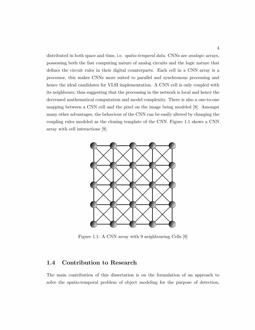
coupling rules modeled as the cloning template of the CNN. Figure 1.1 shows a CNN
array with cell interactions [9].
Figure 1.1: A CNN array with 9 neighbouring Cells [9]
1.4 Contribution to Research
The main contribution of this dissertation is on the formulation of an approach to
solve the spatio-temporal problem of object modeling for the purpose of detection,
5
segmentation, extraction and classification in multiple object scenes with emphasis to
reduce model complexity, increase computational speed and create an easy-to-implement
method of training and classification using CNNs. To achieve this contribution we
address the problems stated in section 1.1. The inspiration to undertake this research
was derived from an observation that most existing spatio-temporal solutions do not
address the problem of complexity of the model. There is also a rising need to implement
visual processing tasks on-chip, which in turn demands that the model complexity is
reduced in order to work in harmony with the chip resources. The reduction of the model
complexity involves choosing a modeling technique that best suits the application, and
the best algorithm that increases memory efficiency and computational speed while
maintaining high accuracy. For this reason, Cellular Neural Networks (CNN) were
chosen as a platform for computing. Through examining the reported work in the
field of CNNs, it was noted that there has not been more focus on the methods of
handling classification of multiple objects/features appearing on one image scene [63].
The available work only lay foundations as to how isolated objects can be classified, but
however does not take into account that learning object features may be more effective
if the environment in which the object appears in is taken into account. This document
formulates the techniques in the Cellular Neural Network domain that can be used to
achieve models of the objects and the application of optimisation techniques to improve
the model performance for applications in object detection, extraction and classification
based on multiple object scenes.
1.5 Objectives
This document proposes the methods of handling object modeling and computation
in multiple object scenarios for the purpose of detection, segmentation, extraction and
classification. Within this main objective, there are several sub-objectives that must
be fulfilled. The following are the sub-objectives through which the main objective is
achieved:
(a) define multiple object classification in terms of modeling and complexity. This
gives answers to the possible causes of model complexity and how artificial intel-
ligent techniques can be employed to reduce the complexity.
6
(b) device techniques through which an efficient object model can be achieved and
accounted for. This follows an exploration of possible CNN techniques that can
be integrated to yield an algorithm that can solve the problem defined on the
point above. This involves evaluation of certain approaches and the adoption of
others owing to their suitability and applicability to spatio-temporal modeling.
(c) formulate optimisation techniques that best optimizes the object models achieved
by the chosen modeling technique. Selecting the best method for optimization
implies the achievement of a global solution that best captures all the object
traits. A selection of an inadequate method result in the solution trapped in local
maxima.
(d) to create an easy-to-implement algorithm for the training and classification of
objects modeled using CNNs. This will serve to indicate the possible advantages
of the choice of CNNs as the proper model for the application of object detection,
extraction and classification.
(e) design an object-based algorithm that consists of reusable parts for all tasks i.e.
segmentation, extraction and classification. This means that a task that is required
by both CNN based image processing tasks is implemented in a polymorphic
approach.
(f) integrate all the algorithm parts into a single analogic framework that defines how
multiple object scenarios are handled using CNNs.
(g) develop a proof-of-concept application that demonstrates the strength of the al-
gorithm proposed in this research work. This objective seeks to demonstrate how
the proposed methods can be applied to solve practical problems.
(h) develop an analysis procedure that is to be used to determine the performance of
the model. Here the accuracy, efficiency and resource intensiveness of the proposed
methods are determined in order to numerically scale their performance.
7
1.6 Chapters and their Respective Contribution
This dissertation is organized into chapters each serving one or more objectives detailed
above. While Chapter 2 builds up a background required to understand the main
direction of this research, the rest of the chapters build up the solution to the problem
of multiple object scenario handling, with each chapter focusing on a specific building
block of the entire solution proposed. The following is a brief discussion on the content
and objectives of each chapter:
1. Chapter 2 gives a thorough background to CNNs. In this chapter the CNN
architecture and its dynamics are presented. The suitability of the architecture to
the spatio-temporal applications is explored and its limitations in general. This
will involve a look at some practical images and their corresponding CNN models.
2. Chapter 3 The objective of this chapter is to formulate and present a series of
CNN based image processing tasks that allow the object to be separated from the
background and other objects in the image without altering its features. In order
to achieve this we employ image processing methods such as nonlinear diffusion,
CNN based thresholding and edge detection. A successful extraction technique
leads to the image model that can be used during learning and classification.
3. Chapter 4 presents various strategies that can be used to select the features
that best represent the object being studied. This chapter deals mainly with how
the object features are represented as sets of stable memories and stored in the
CNN templates. This chapter also presents the types of CNN networks that can
be used for learning object features. Several features that are regarded as more
distinctive to objects will also be examined. Of this we study texture through
texture histograms and apply heuristics to design bounds for texture classes.
4. Chapter 5 is an integration of all the chapters above into analogic algorithms that
can be used to train the CNN to classify objects. The algorithm proposed here is
general and can be adopted to different application scenarios. Two algorithms are
proposed, namely (1) genetically optimized CNNs for feature learning and texture
histograms for boundary conditions design for class objects.
8
5. Chapter 6 gives an introduction to some practical examples where the proposed
algorithms are applicable. Example 1 is a practical application of the algorithm
designed during this research and submitted to the International Association of
Science and Technology for Development(IASTED). This example is in the clas-
sification of satellite sensed data using genetically optimized CNNs. Another
example presented is on the use of diffusion filtered and modified histograms to
perform texture based classification of objects based on multiple texture object
scenes. This chapter further details the analysis procedure to be used to evaluate
the performance of the algorithms proposed in this document. The procedure in-
volves setting up certain standards of acceptability for any algorithm in this case
by looking at measures of efficiency such as memory utilisation, processing time,
percentage accuracy and applicability in real world problems.
6. Chapter 7 summarizes all the chapters by looking back at the goals set in section
1.5. It further details the impact of this research to the modern world and paves
way to challenges in this research that require further investigation. The chapter
also gives the weight of the material covered in this research in terms of originality
and referencing.
Chapter 2
CNNs in Image Processing
2.1 Local Processing, Coupling and Nonlinear Dynamics
In the introduction of the CNNs a paradigm of complexity, a CNN is defined as a regular
array of MXN dimensions composed of nonlinear units with only local interaction
within a neighbourhood radius [5,6]. The most distinctive features of this model are [8]:
1. local processing, which ensures that all cell interactions are local (i.e. within
each cell and its neighbours). This decreases the complexity of the model.
2. coupling, defines the rules of cell interactions within the neighbouring cells. The
behavior of the network is altered by changing these rules. The complexity of the
model increases if there is no coupling in the network. Uncoupled cells in an array
can present chaos and instability. The relational rules for mapping input and
output becomes difficult to model and define when there is no inter-relationships
between local cells [9].
3. nonlinear dynamics, define the nature of the processing elements, the cells.
“dynamic” implies the dependency of the cells on the state of the neighbouring
cells, while “nonlinear” defines the nature of the output activation caused by the
Chua-Yang’s choice of the piecewise-linear function.
In analogy to the universe, local processing describes the dynamics and functioning of
the smallest building blocks of matter, the cells, while coupling defines the the influence
9
10
that neighbouring cells have on the state of the cell and propagation of the cell behaviour
throughout the entire universe to give it an overall dynamic behavior. Through coupling
and local interaction, the dynamics of very complex nonlinear systems can be modeled
and analysed. Section 2.2 introduces one of such models for complexity introduced by
Chua and Yang in [5].
2.2 The Chua-Yang CNN Model
The idea proposed by Chua and Yang to address the problem of complexity was to
use an array of dynamical cells to process a large amount of data in real time [1].
Processing data in real time require analog processors, while processing large amounts
of data may require parallel synchronous processors. This supports their choice of a
cellular array wherein each cell is an analog processor that serves as an input-output
stage of the network. In order to control the behaviour of the model with respect
to the dynamic range and stability, Chua and Yang apply logic theory that is widely
used in digital circuits. This result into a computer that possesses both the speed and
computational power of analogue and digital circuits, which is presently known as the
Analogic Computer [10].
In the original Chua-Yang model, the neighbourhood, r, of a dynamical cell in the i -th
row and the j -th column, termed Cij , on an M X N CNN array is defined by:
N rij = { Ckl|max{|k − i|, |l − j|} ≥ r; 1 ≤ k ≤ N1, 1 ≤ l ≤ N2} (2.1)
where r is a positive integer, and i and j are row and column indexes respectively
[5,6,7,10].
Each cell of the CNN has a continuous valued state variable x, an input variable u,
and the output y. The nonlinear dynamics of the CNN is defined by the following set
of equations:
Cdxij(t)
dt= − 1
Rxij(t) +
∑CklεN
rij
A(i, j; k, l)ykl(t) +∑
CklεNrij
B(i, j; k, l)ukl + Iij
and
yij(t) =12(|xij(t) + 1| − |xij(t)− 1|) (2.2)
11
where C and R are integral constants of the system, xij is the state of a cell, I is an
independent bias constant, and yij is the activation function [5,7].
The matrices A and B that operate on the input and the output respectively are called
the Cloning Templates or the CNN Kernel. The former acts as feedback template and
the latter as an input control template [5,8,10]. The cloning template represented by A
and B may be linear or nonlinear, space variable or invariable depending on the appli-
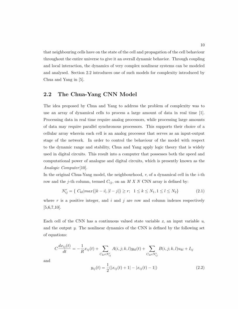
cation. The output function of the CNN is chosen based on the desired application of
the CNN. [5] and [10] lists the following output activation functions and their areas of
application:
1. piecewise-linear model - shown in equation 2.2.
2. nonlinearity model - most applicable to on-chip VLSI
3. hyperbolic function - used for training applications where the learning follows the
gradient descent rule.
The activation functions described above are as shown in Figure 2.1.
Figure 2.1: The learning functions used in the CNN output activation:(a) the piecewise-linear model, (b) the nonlinearity model and (c) the tangential hyperbolic function [9]
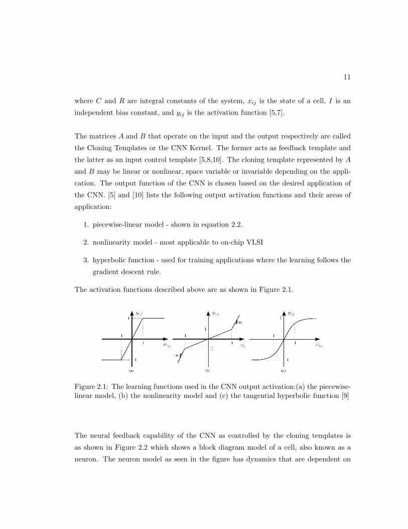
The neural feedback capability of the CNN as controlled by the cloning templates is
as shown in Figure 2.2 which shows a block diagram model of a cell, also known as a
neuron. The neuron model as seen in the figure has dynamics that are dependent on
12
Figure 2.2: The block diagram depicting the signal flow on a CNN Cell [11]
coupling rules set on the templates A and B.
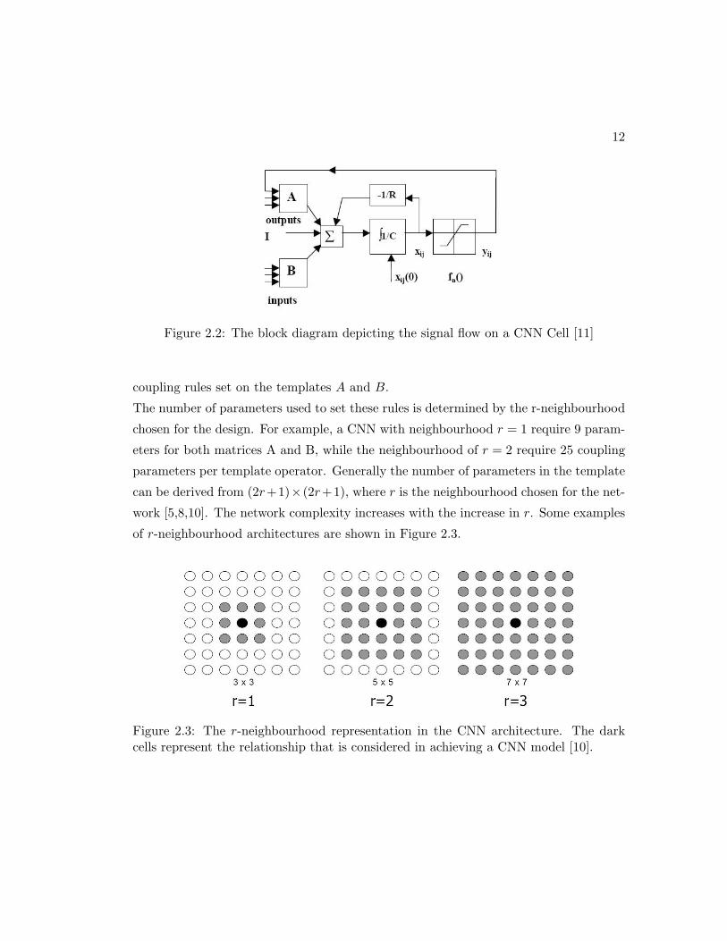
The number of parameters used to set these rules is determined by the r-neighbourhood
chosen for the design. For example, a CNN with neighbourhood r = 1 require 9 param-
eters for both matrices A and B, while the neighbourhood of r = 2 require 25 coupling
parameters per template operator. Generally the number of parameters in the template
can be derived from (2r+1)×(2r+1), where r is the neighbourhood chosen for the net-
work [5,8,10]. The network complexity increases with the increase in r. Some examples
of r-neighbourhood architectures are shown in Figure 2.3.
Figure 2.3: The r-neighbourhood representation in the CNN architecture. The darkcells represent the relationship that is considered in achieving a CNN model [10].

13
2.2.1 CNN Classes
The most categorizing parameter of a CNN is the cloning template . With alteration
of the cloning template, a wide range of CNNs with unique behaviours are defined.
However, Chua and Roska define three classes from which all the subclasses inherit
their behaviour [10].
(a). Zero-Feedback or Feedforward CNNs
A CNN that belongs to this class is defined by the following equation:
Cdxij(t)
dt= − 1
Rxij(t) +
∑CklεN
rij
B(i, j; k, l)ukl + Iij (2.3)
This class is characterized by an uncoupled behaviour between the input of the network
and the corresponding output. The signal flow system structure associated with the cell
forming this type of network is shown in Figure 2.4.
Figure 2.4: The system structure depicting the signal flow of the zero-feedback CNNcell [10]
(b). Zero-Input CNNs
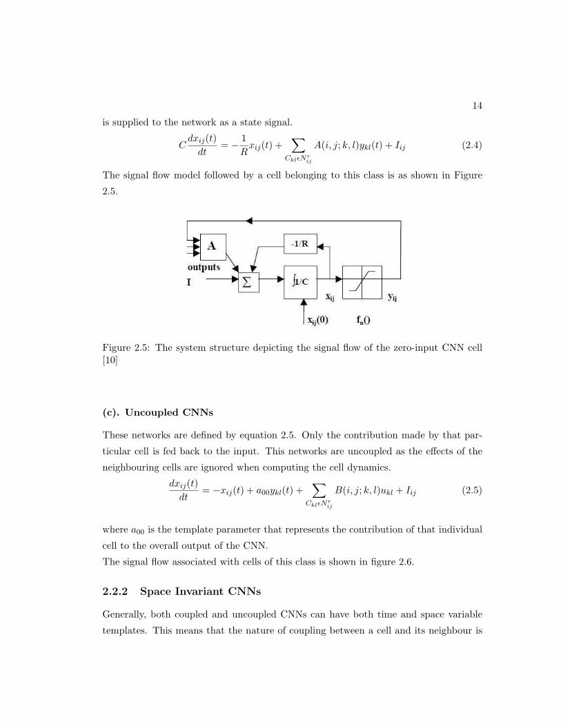
A CNN belonging to this class is defined by equation 2.4. This network does not take
any input as there is no input control template (i.e the B template is zero). The input
14
is supplied to the network as a state signal.
Cdxij(t)
dt= − 1
Rxij(t) +
∑CklεN
rij
A(i, j; k, l)ykl(t) + Iij (2.4)
The signal flow model followed by a cell belonging to this class is as shown in Figure
2.5.
Figure 2.5: The system structure depicting the signal flow of the zero-input CNN cell[10]
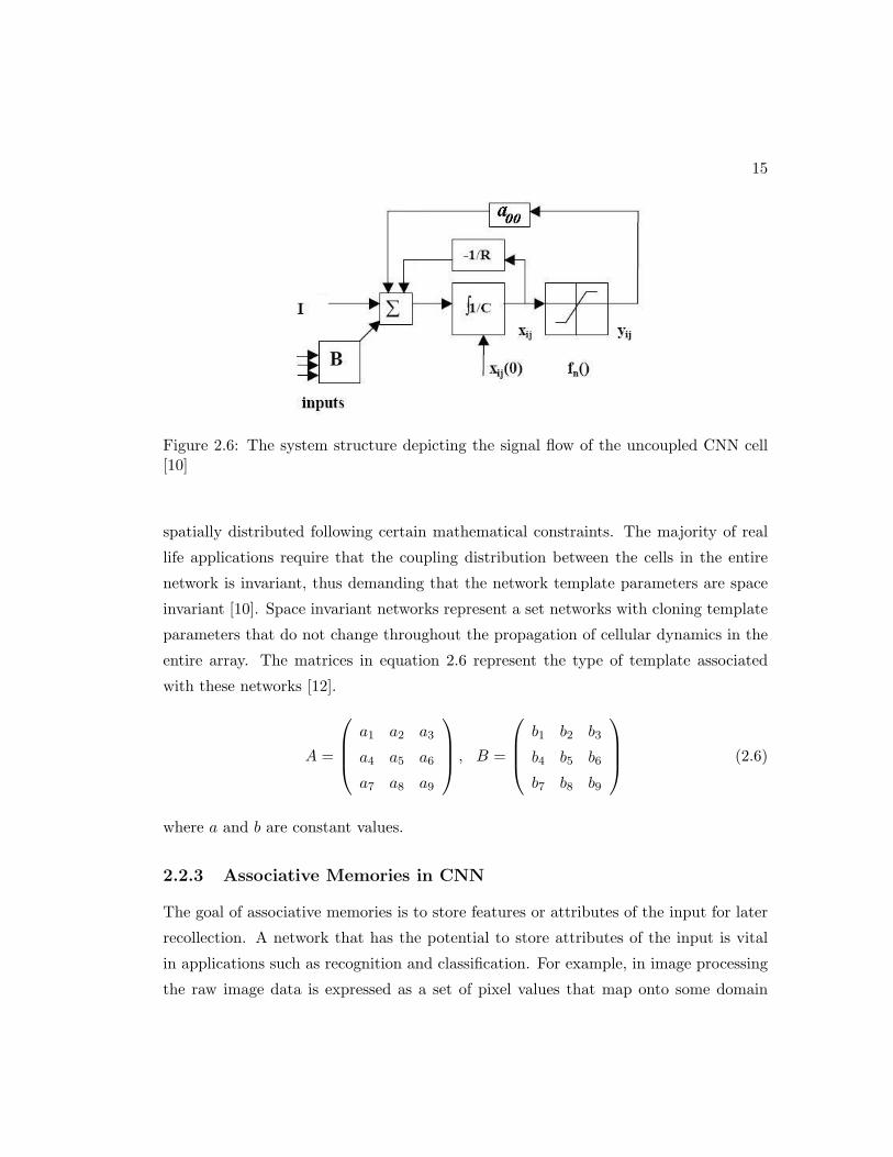
(c). Uncoupled CNNs
These networks are defined by equation 2.5. Only the contribution made by that par-
ticular cell is fed back to the input. This networks are uncoupled as the effects of the
neighbouring cells are ignored when computing the cell dynamics.
dxij(t)dt
= −xij(t) + a00ykl(t) +∑
CklεNrij
B(i, j; k, l)ukl + Iij (2.5)
where a00 is the template parameter that represents the contribution of that individual
cell to the overall output of the CNN.
The signal flow associated with cells of this class is shown in figure 2.6.
2.2.2 Space Invariant CNNs
Generally, both coupled and uncoupled CNNs can have both time and space variable
templates. This means that the nature of coupling between a cell and its neighbour is
15
Figure 2.6: The system structure depicting the signal flow of the uncoupled CNN cell[10]
spatially distributed following certain mathematical constraints. The majority of real
life applications require that the coupling distribution between the cells in the entire
network is invariant, thus demanding that the network template parameters are space
invariant [10]. Space invariant networks represent a set networks with cloning template
parameters that do not change throughout the propagation of cellular dynamics in the
entire array. The matrices in equation 2.6 represent the type of template associated
with these networks [12].
A =
a1 a2 a3
a4 a5 a6
a7 a8 a9
, B =
b1 b2 b3
b4 b5 b6
b7 b8 b9
(2.6)
where a and b are constant values.
2.2.3 Associative Memories in CNN
The goal of associative memories is to store features or attributes of the input for later
recollection. A network that has the potential to store attributes of the input is vital
in applications such as recognition and classification. For example, in image processing
the raw image data is expressed as a set of pixel values that map onto some domain
16
that may represent an edge or some other features that distinctively characterize the
object or one of its class. The goal of an associative processor in this case is to asso-
ciate any other input that it has never learned with the one of its kind that has been
learned. Generation of associative memories in the CNN architecture means the design
of coupling rules between each cell and its neighbours that can be stored as kernel maps
(template) for the recollection of a particular input pattern [13].
There are several methods of implementing associative memories in CNNs. Szolgay
et al [14] propose a fixed point learning method for associative memory design with
space varying templates. The design is based on the autonomous (Zero-input) CNN
model defined in section 2.2.1. The method is based on computing the cost function
that provides the best convergence speed. During learning the equilibrium state of a cell
should be located outside the region of saturation. For this condition to be sufficient,
the magnitude of the equilibrium point is evaluated by equation 2.7.
Enij = AT
ij .pnij + Iij .y
nij : En
ij ≤ E ≤ 1 (2.7)
where n = 1, , , , p;i = 1, , ,M ;j = 1, , , N and E is the constant around which magnitude
of an equilibrium point of a cell is set.
With the satisfaction of the condition in equation 2.7, Szolgay et al uses the Herbial
Lerning Rule to compute the matrix Aij using a weighting factor Wnij of the nth pattern
as shown in equation 2.8.
Aij =p∑
n=1
Wnij .p
nij (2.8)
Using the Zero-input network, Liu and Lu [15] propose a procedure for the synthesis of
space invariant CNN templates. The design algorithm is based on the eigenstructure
method where a set matrices representing cloning template parameters of the Network
are derived through singular value decomposition. The method is implemented with a
view of the perceptron learning algorithm to ensure convergence at an optimal solution
(i.e. termination of algorithm with stable memories)
17
The synthesis procedure for this approach is based on the discrete time CNN model
with the following set equations:
x = −xij + Tij,klsat(x) + Iij where yij = sat(x) (2.9)
where A is chosen to be an identity matrix, Tij,kl is the feedback cloning template and
Iij is the threshold or bias current.
There are several comparisons that can be drawn between the CNN associative model
and its Hopfield counterpart. While the weights of the hopfield network are computed
through a herbian rule, the CNN learning is not limited to any specific rule. The
Hopfield model operates asynchronously, whereas the CNN model can operate in a syn-
chronous mode. Due to local connectivity, the interconnection matrix that is required
to store the stable memories in the CNN is very small. A fully connected hopfield net-
work require more space to store all interconnection weights between the inputs, hidden
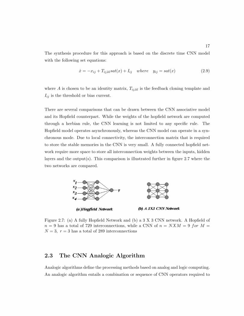
layers and the output(s). This comparison is illustrated further in figure 2.7 where the
two networks are compared.
Figure 2.7: (a) A fully Hopfield Network and (b) a 3 X 3 CNN network. A Hopfield ofn = 9 has a total of 729 interconnections, while a CNN of n = NXM = 9 for M =N = 3, r = 3 has a total of 289 interconnections
2.3 The CNN Analogic Algorithm
Analogic algorithms define the processing methods based on analog and logic computing.
An analogic algorithm entails a combination or sequence of CNN operators required to
18
solve a complex problem in real time. For example, the necessary steps required to
perform CNN-based image morphology are implemented as a series of CNN operators.
Analogic algorithm implies the application of one or more CNN space and/or time
variant/invariant template(s) to an input in a predefined sequence and time to generate
a spatio-temporal solution. These algorithms are key to the formulation of a CNN based
solution to spatio-temporal problems. By altering the cloning templates of a network
at specific times and order, the input parameters are processed into some output that
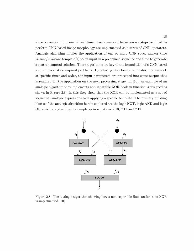
is required for the application on the next processing stage. In [10], an example of an
analogic algorithm that implements non-separable XOR boolean function is designed as
shown in Figure 2.8. In this they show that the XOR can be implemented as a set of
sequential analogic expressions each applying a specific template. The primary building
blocks of the analogic algorithm herein explored are the logic NOT, logic AND and logic
OR which are given by the templates in equations 2.10, 2.11 and 2.12.
Figure 2.8: The analogic algorithm showing how a non-separable Boolean function XORis implemented [10]
19
(i). The logic NOT
A =
0 0 0
0 1 0
0 0 0
, B =
0 0 0
0 −2 0
0 0 0
, I = 0 (2.10)
(ii). The logic AND
A =
0 0 0
0 2 0
0 0 0
, B =
0 0 0
0 2 0
0 0 0
, I = −2 (2.11)
(iii). The logic OR
A =
0 0 0
0 2 0
0 0 0
, B =
0 0 0
0 2 0
0 0 0
, I = 2 (2.12)
2.4 The Adoption of the CNN Architectures for Image
Processing
Image processing involves the manipulation of the visual and non-visual aspects of an
image with a goal of extracting and studying the information contained in it. Image
processing is a well developed field and has found application in areas such as visual
quality inspection, tracking, pattern recognition and visual classification. Though ar-
tificial intelligent models have been found to be more accurate, most of them do not
address the problem of complexity, memory and computational speed. The emergence
of CNNs have introduced a paradigm of solving complex image processing problems
with increased computational speed and reduction of memory utilisation [1].
Since inception, the CNN architecture has been actively researched for application to
spatio-temporal processing and industries have witnessed the realisation of VLSI-based
visual processors. The simplicity of the CNN architecture has attracted more research
for applicability in visual computing. Highly complex image models have been designed
using CNNs, for example the CNN retina model [16][17], the DNA microprocessor arrays
20
[1] and Cellular Wave Computers for Brain-like Spatial-temporal Sensory Computing
[18]. Wang et al [19] investigated the use of CNNs to perform object segmentation
in image sequence, taking advantage of the image statistical data. That is, by map-
ping the image spatial domain to its statistical domain, a robust image segmentation
method can be achieved even in cases of changing background. Szabo and Szolgay [20]
have described an analogic-based (CNN) diffusion algorithm for segmentation of image
by performing CNN-based binary mathematical morphology. The use of bayesian tech-
niques combined with CNNs has also been proposed by many researchers. Milanova,
Elmaghraby and Rubin [11] have discussed the MRF-based method which takes ad-
vantage of the Maximum of a posteriori (MAP) and the CNN energy function. This
method also tries to map the CNN model of an image onto its statistical representation.
There are many CNN templates that exist to handle the image segmentation in different
imaging environments.
Various methods of using CNNs in feature extraction and classification have also been
reported in many publications. Rekeczky et al [21] have developed a framework for
a cellular (visual) sensor computer which performs feature detection based on terrain
classification; and motion analysis based on navigation parameter estimation. In [22]
and [23], Rekeczky et al also detail a method of feature extraction by computing topo-
graphic feature maps from video terrain flows, feature selection by Principal Component
Analysis (PCA) and Decision Trees; and feature classification using Nearest Neighbor
Family (NNF) methods.
Optimization techniques have also been deployed to enhance techniques of feature detec-
tion in CNN architectures. Vandewalle and Dellaert [24] outline a method for automatic
design of CNNs using Genetic Algorithms (GAs) to perform image feature detection.
In order to perform classification using CNN templates, a synthesis of autoassociative
memory (as in the case of Hopfield Networks) is essential. CNN associative memory for
feature recall and classification purposes is achieved through design procedures that try
to mimic the nature of associative recall in Hopfield Networks. [14,15,24] and [25] pro-
pose a variety of methods such as GAs, fixed-point learning and eigenstructure methods
which can be used in template design for associative memories.
These applications unleash CNNs as networks highly suited for complex systems mod-
eling and analysis. In Chapter 3, the use of these networks to derive models for objects
21
embedded in multiple object scenarios is explored. The accurate models in these case
are achieved through accurate detection, segmentation and extraction of the object from
the scene in order to study the object in isolation.
Chapter 3
Multiple Object Scenario
Modeling using CNNs
This chapter forms the base of the proposed algorithms for dealing with object modeling
in multiple object scenes. For the purpose of this chapter, a definition of a “multiple
object” scene is outlined first, with emphasis to the inherent complexities in modeling
objects in multiple object views. This chapter extends the available methods for the
designing analogic algorithms that are suitable for this task. The first step required
for a successful model is the filtering stage that normalizes the image and enhance
the pixel intensities to ensure consistency. Various techniques of image filtering are
introduced. The importance of computing statistical tools such as mean, variance,
diffusion and threshold images is also evaluated. The object model is considered accurate
if it successfully leads to an accurate extraction of that object from the scene. In this
chapter, the focus is mainly on the development of analogic algorithms that output the
extracted object. These algorithms are based on the image operators mentioned herein
(i.e. mean, variance etc). With a successful extraction algorithm, a CNN model of the
object can be achieved.
3.1 Defining a Multiple Object Scene
Consider the problem of learning about one object which can appear at various locations
in an image. The object is in the foreground, with a background behind it. This
22
23
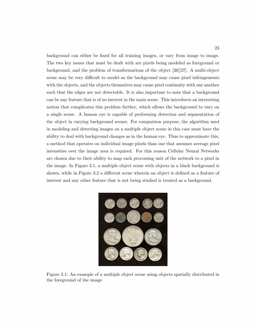
background can either be fixed for all training images, or vary from image to image.
The two key issues that must be dealt with are pixels being modeled as foreground or
background, and the problem of transformations of the object [26][27]. A multi-object
scene may be very difficult to model as the background may cause pixel infringements
with the objects, and the objects themselves may cause pixel continuity with one another
such that the edges are not detectable. It is also important to note that a background
can be any feature that is of no interest in the main scene. This introduces an interesting
notion that complicates this problem further, which allows the background to vary on
a single scene. A human eye is capable of performing detection and segmentation of
the object in varying background scenes. For comparison purpose, the algorithm used
in modeling and detecting images on a multiple object scene in this case must have the
ability to deal with background changes as in the human eye. Thus to approximate this,
a method that operates on individual image pixels than one that assumes average pixel
intensities over the image area is required. For this reason Cellular Neural Networks
are chosen due to their ability to map each processing unit of the network to a pixel in
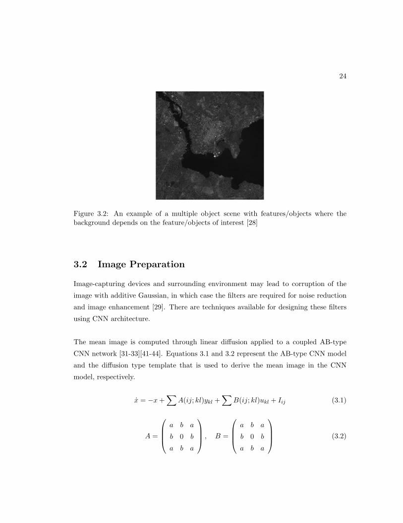
the image. In Figure 3.1, a multiple object scene with objects in a black background is
shown, while in Figure 3.2 a different scene wherein an object is defined as a feature of
interest and any other feature that is not being studied is treated as a background.
Figure 3.1: An example of a multiple object scene using objects spatially distributed inthe foreground of the image
24
Figure 3.2: An example of a multiple object scene with features/objects where thebackground depends on the feature/objects of interest [28]
3.2 Image Preparation
Image-capturing devices and surrounding environment may lead to corruption of the
image with additive Gaussian, in which case the filters are required for noise reduction
and image enhancement [29]. There are techniques available for designing these filters
using CNN architecture.
The mean image is computed through linear diffusion applied to a coupled AB-type
CNN network [31-33][41-44]. Equations 3.1 and 3.2 represent the AB-type CNN model
and the diffusion type template that is used to derive the mean image in the CNN
model, respectively.
x = −x +∑
A(ij; kl)ykl +∑
B(ij; kl)ukl + Iij (3.1)
A =
a b a
b 0 b
a b a
, B =
a b a
b 0 b
a b a
(3.2)
25
where 0 ≤ a, b ≤ 1
The variance of the image in the CNN domain is computed through the average dif-
ference method implemented as a nonlinear B-type template or the Laplace [32]. The
network of this type is as represented in equation 3.3.
xij = −xij +∑
B(ij; kl)(∆ukl) +∑
B(ij; kl)(∆ukl) + Iij (3.3)
where B is the nonlinear input control template.
The CNN template associated with the architecture defined by equation 3.3 is shown
in equation 3.2.
Bb =1n
1 1 1
1 0 1
1 1 1
,
b = [interp pnum x1y1, x2y2 . . . xnyn] (3.4)
where A = 0, A = 0, nε< > 1 is the scaling factor, interp is the interpolation method
(i.e. piecewise constant or piecewise linear), pnum is the number of points and x1y1
. . .xnyn are the interpolation points.
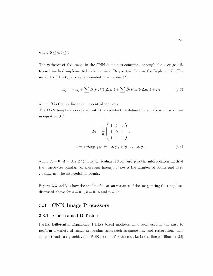
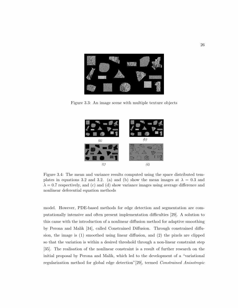
Figures 3.3 and 3.4 show the results of mean an variance of the image using the templates
discussed above for a = 0.1, b = 0.15 and n = 16.
3.3 CNN Image Processors
3.3.1 Constrained Diffusion
Partial Differential Equations (PDEs) based methods have been used in the past to
perform a variety of image processing tasks such as smoothing and restoration. The
simplest and easily achievable PDE method for these tasks is the linear diffusion [33]
26
Figure 3.3: An image scene with multiple texture objects
Figure 3.4: The mean and variance results computed using the space distributed tem-plates in equations 3.2 and 3.2. (a) and (b) show the mean images at λ = 0.3 andλ = 0.7 respectively, and (c) and (d) show variance images using average difference andnonlinear deferential equation methods
model. However, PDE-based methods for edge detection and segmentation are com-
putationally intensive and often present implementation difficulties [29]. A solution to
this came with the introduction of a nonlinear diffusion method for adaptive smoothing
by Perona and Malik [34], called Constrained Diffusion. Through constrained diffu-
sion, the image is (1) smoothed using linear diffusion, and (2) the pixels are clipped
so that the variation is within a desired threshold through a non-linear constraint step
[35]. The realisation of the nonlinear constraint is a result of further research on the
initial proposal by Perona and Malik, which led to the development of a “variational
regularization method for global edge detection”[29], termed Constrained Anisotropic
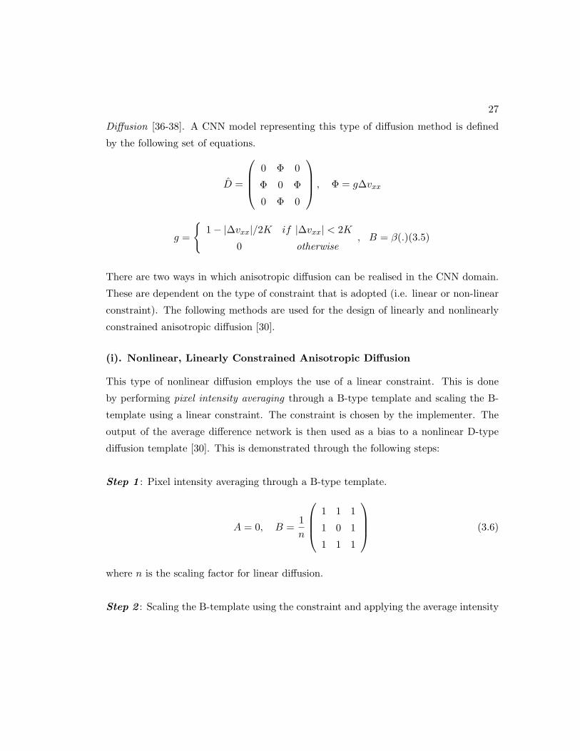
27
Diffusion [36-38]. A CNN model representing this type of diffusion method is defined
by the following set of equations.
D =
0 Φ 0
Φ 0 Φ
0 Φ 0
, Φ = g∆vxx
g =
{1− |∆vxx|/2K if |∆vxx| < 2K
0 otherwise, B = β(.)(3.5)
There are two ways in which anisotropic diffusion can be realised in the CNN domain.
These are dependent on the type of constraint that is adopted (i.e. linear or non-linear
constraint). The following methods are used for the design of linearly and nonlinearly
constrained anisotropic diffusion [30].
(i). Nonlinear, Linearly Constrained Anisotropic Diffusion
This type of nonlinear diffusion employs the use of a linear constraint. This is done
by performing pixel intensity averaging through a B-type template and scaling the B-
template using a linear constraint. The constraint is chosen by the implementer. The
output of the average difference network is then used as a bias to a nonlinear D-type
diffusion template [30]. This is demonstrated through the following steps:
Step 1 : Pixel intensity averaging through a B-type template.
A = 0, B =1n
1 1 1
1 0 1
1 1 1
(3.6)
where n is the scaling factor for linear diffusion.
Step 2 : Scaling the B-template using the constraint and applying the average intensity
28
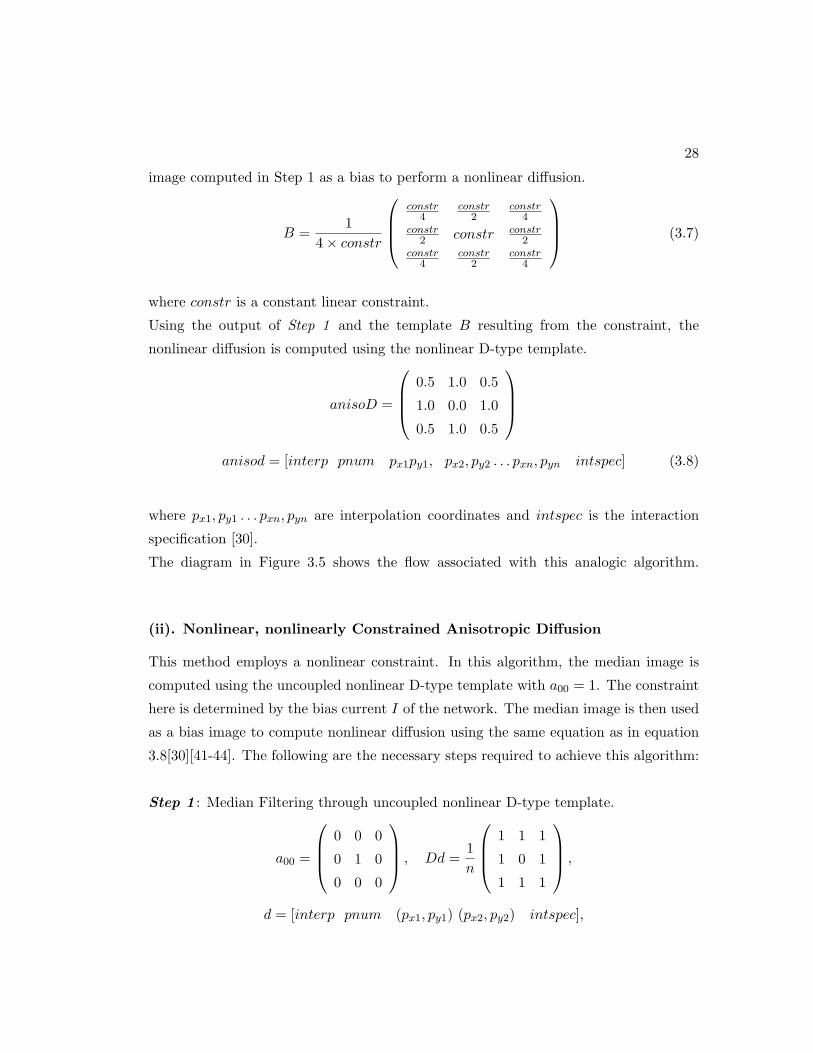
image computed in Step 1 as a bias to perform a nonlinear diffusion.
B =1
4× constr
constr
4constr
2constr
4constr
2 constr constr2
constr4
constr2
constr4
(3.7)
where constr is a constant linear constraint.
Using the output of Step 1 and the template B resulting from the constraint, the
nonlinear diffusion is computed using the nonlinear D-type template.
anisoD =
0.5 1.0 0.5
1.0 0.0 1.0
0.5 1.0 0.5
anisod = [interp pnum px1py1, px2, py2 . . . pxn, pyn intspec] (3.8)
where px1, py1 . . . pxn, pyn are interpolation coordinates and intspec is the interaction
specification [30].
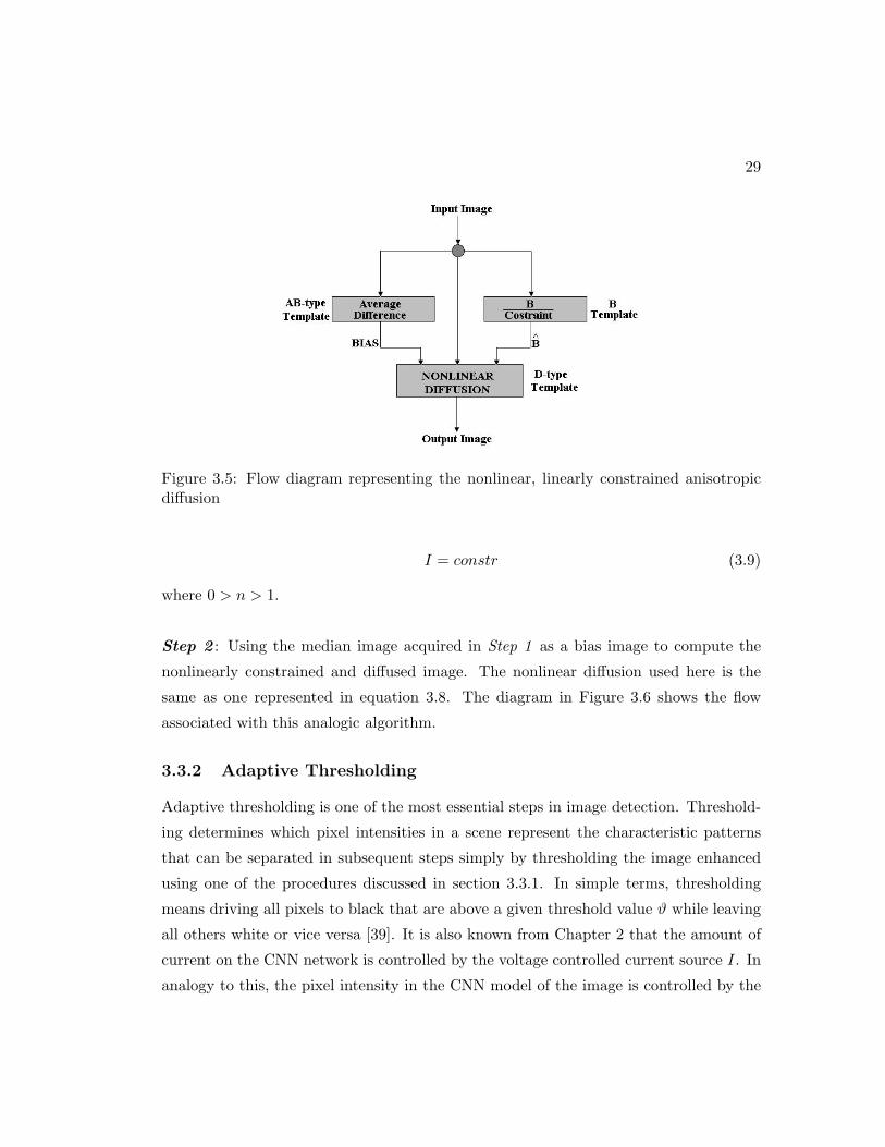
The diagram in Figure 3.5 shows the flow associated with this analogic algorithm.
(ii). Nonlinear, nonlinearly Constrained Anisotropic Diffusion
This method employs a nonlinear constraint. In this algorithm, the median image is
computed using the uncoupled nonlinear D-type template with a00 = 1. The constraint
here is determined by the bias current I of the network. The median image is then used
as a bias image to compute nonlinear diffusion using the same equation as in equation
3.8[30][41-44]. The following are the necessary steps required to achieve this algorithm:
Step 1 : Median Filtering through uncoupled nonlinear D-type template.
a00 =
0 0 0
0 1 0
0 0 0
, Dd =1n
1 1 1
1 0 1
1 1 1
,
d = [interp pnum (px1, py1) (px2, py2) intspec],
29
Figure 3.5: Flow diagram representing the nonlinear, linearly constrained anisotropicdiffusion
I = constr (3.9)
where 0 > n > 1.
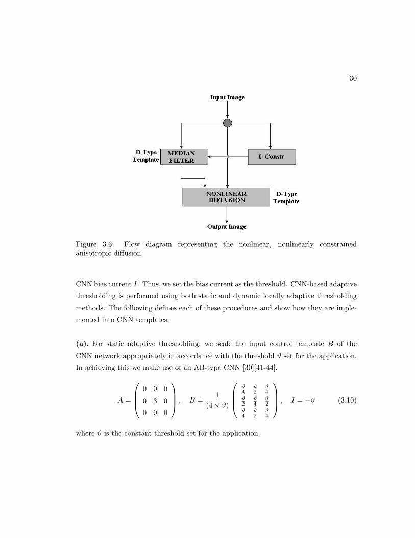
Step 2 : Using the median image acquired in Step 1 as a bias image to compute the
nonlinearly constrained and diffused image. The nonlinear diffusion used here is the
same as one represented in equation 3.8. The diagram in Figure 3.6 shows the flow
associated with this analogic algorithm.
3.3.2 Adaptive Thresholding
Adaptive thresholding is one of the most essential steps in image detection. Threshold-
ing determines which pixel intensities in a scene represent the characteristic patterns
that can be separated in subsequent steps simply by thresholding the image enhanced
using one of the procedures discussed in section 3.3.1. In simple terms, thresholding
means driving all pixels to black that are above a given threshold value ϑ while leaving
all others white or vice versa [39]. It is also known from Chapter 2 that the amount of
current on the CNN network is controlled by the voltage controlled current source I. In
analogy to this, the pixel intensity in the CNN model of the image is controlled by the
30
Figure 3.6: Flow diagram representing the nonlinear, nonlinearly constrainedanisotropic diffusion
CNN bias current I. Thus, we set the bias current as the threshold. CNN-based adaptive
thresholding is performed using both static and dynamic locally adaptive thresholding
methods. The following defines each of these procedures and show how they are imple-
mented into CNN templates:
(a). For static adaptive thresholding, we scale the input control template B of the
CNN network appropriately in accordance with the threshold ϑ set for the application.
In achieving this we make use of an AB-type CNN [30][41-44].
A =
0 0 0
0 3 0
0 0 0
, B =1
(4× ϑ)
ϑ4
ϑ2
ϑ4
ϑ2
ϑ4
ϑ2
ϑ4
ϑ2
ϑ4
, I = −ϑ (3.10)
where ϑ is the constant threshold set for the application.
31
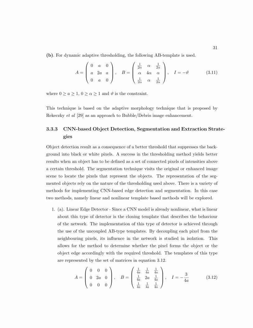
(b). For dynamic adaptive thresholding, the following AB-template is used.
A =
0 a 0
a 2a a
0 a 0
, B =
12α α 1
2α
α 4α α12α α 1
2α
, I = −ϑ (3.11)
where 0 ≥ a ≥ 1, 0 ≥ α ≥ 1 and ϑ is the constraint.
This technique is based on the adaptive morphology technique that is proposed by
Rekeczky et al [29] as an approach to Bubble/Debris image enhancement.
3.3.3 CNN-based Object Detection, Segmentation and Extraction Strate-
gies
Object detection result as a consequence of a better threshold that suppresses the back-
ground into black or white pixels. A success in the thresholding method yields better
results when an object has to be defined as a set of connected pixels of intensities above
a certain threshold. The segmentation technique visits the original or enhanced image
scene to locate the pixels that represent the objects. The representation of the seg-
mented objects rely on the nature of the thresholding used above. There is a variety of
methods for implementing CNN-based edge detection and segmentation. In this case
two methods, namely linear and nonlinear template based methods will be explored.
1. (a). Linear Edge Detector - Since a CNN model is already nonlinear, what is linear
about this type of detector is the cloning template that describes the behaviour
of the network. The implementation of this type of detector is achieved through
the use of the uncoupled AB-type templates. By decoupling each pixel from the
neighbouring pixels, its influence in the network is studied in isolation. This
allows for the method to determine whether the pixel forms the object or the
object edge accordingly with the required threshold. The templates of this type
are represented by the set of matrices in equation 3.12.
A =
0 0 0
0 2a 0
0 0 0
, B =
14a
14a
14a
14a 2a 1
4a14a
14a
14a
, I = − 34a
(3.12)
32
where a is normally chosen to be greater than 1.
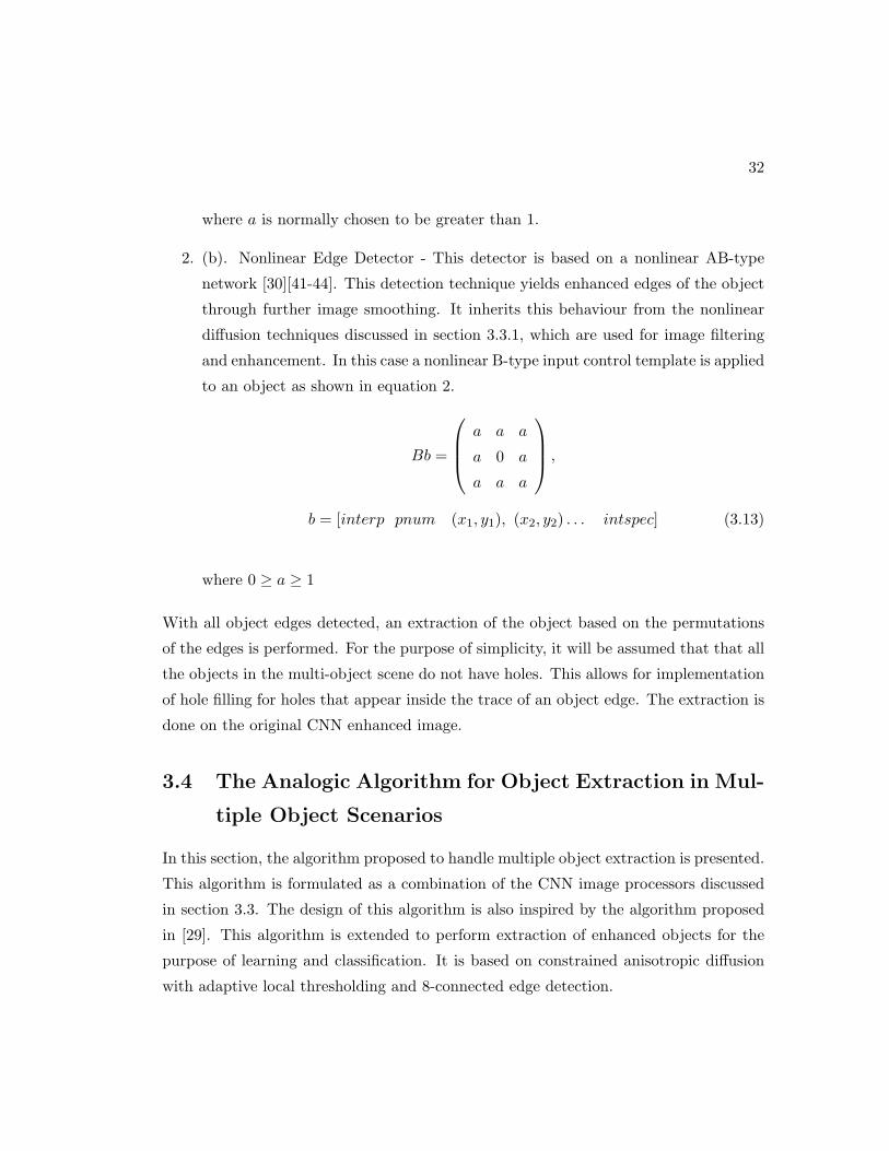
2. (b). Nonlinear Edge Detector - This detector is based on a nonlinear AB-type
network [30][41-44]. This detection technique yields enhanced edges of the object
through further image smoothing. It inherits this behaviour from the nonlinear
diffusion techniques discussed in section 3.3.1, which are used for image filtering
and enhancement. In this case a nonlinear B-type input control template is applied
to an object as shown in equation 2.
Bb =
a a a
a 0 a
a a a
,
b = [interp pnum (x1, y1), (x2, y2) . . . intspec] (3.13)
where 0 ≥ a ≥ 1
With all object edges detected, an extraction of the object based on the permutations
of the edges is performed. For the purpose of simplicity, it will be assumed that that all
the objects in the multi-object scene do not have holes. This allows for implementation
of hole filling for holes that appear inside the trace of an object edge. The extraction is
done on the original CNN enhanced image.
3.4 The Analogic Algorithm for Object Extraction in Mul-
tiple Object Scenarios
In this section, the algorithm proposed to handle multiple object extraction is presented.
This algorithm is formulated as a combination of the CNN image processors discussed
in section 3.3. The design of this algorithm is also inspired by the algorithm proposed
in [29]. This algorithm is extended to perform extraction of enhanced objects for the
purpose of learning and classification. It is based on constrained anisotropic diffusion
with adaptive local thresholding and 8-connected edge detection.
33
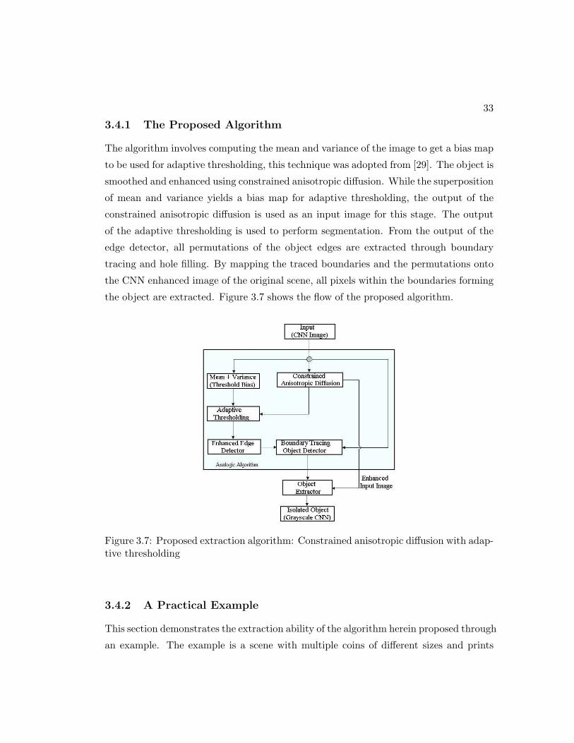
3.4.1 The Proposed Algorithm
The algorithm involves computing the mean and variance of the image to get a bias map
to be used for adaptive thresholding, this technique was adopted from [29]. The object is
smoothed and enhanced using constrained anisotropic diffusion. While the superposition
of mean and variance yields a bias map for adaptive thresholding, the output of the
constrained anisotropic diffusion is used as an input image for this stage. The output
of the adaptive thresholding is used to perform segmentation. From the output of the
edge detector, all permutations of the object edges are extracted through boundary
tracing and hole filling. By mapping the traced boundaries and the permutations onto
the CNN enhanced image of the original scene, all pixels within the boundaries forming
the object are extracted. Figure 3.7 shows the flow of the proposed algorithm.
Figure 3.7: Proposed extraction algorithm: Constrained anisotropic diffusion with adap-tive thresholding
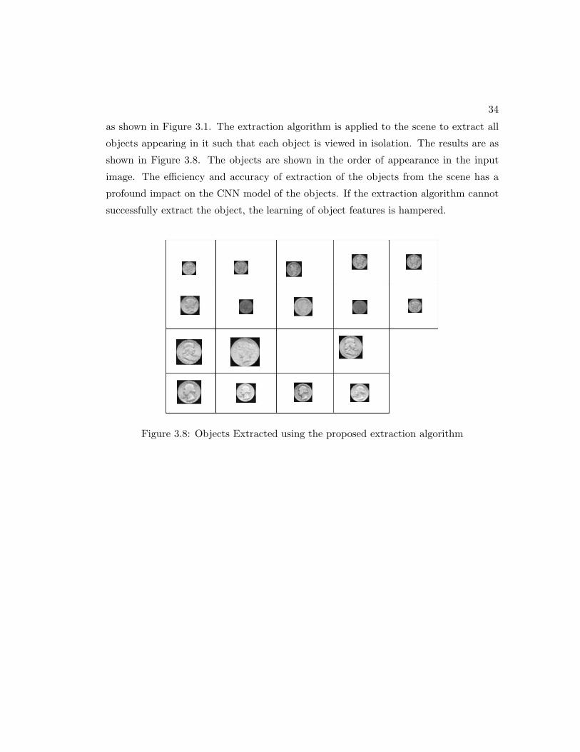
3.4.2 A Practical Example
This section demonstrates the extraction ability of the algorithm herein proposed through
an example. The example is a scene with multiple coins of different sizes and prints
34
as shown in Figure 3.1. The extraction algorithm is applied to the scene to extract all
objects appearing in it such that each object is viewed in isolation. The results are as
shown in Figure 3.8. The objects are shown in the order of appearance in the input
image. The efficiency and accuracy of extraction of the objects from the scene has a
profound impact on the CNN model of the objects. If the extraction algorithm cannot
successfully extract the object, the learning of object features is hampered.
Figure 3.8: Objects Extracted using the proposed extraction algorithm
Chapter 4
Feature Selection and Extraction
Strategies for CNN Classification
Models
The performance of a classification method relies on the art of gathering the most unique
attributes of the learned object. This art can be derived from both mathematical and
analytical methods. In this chapter, some feature extraction strategies are formulated
based on existing theories. Some existing methods will be adopted based on their per-
formance in the field of multiple object learning and classification. The methodologies
for gathering, analysing and manipulating object features to create decision boundaries
are also formulated. This chapter will first outline the strategies used to create decision
boundaries and then further introduces methods of extracting features such as texture,
shape and colour with reference to the storage and representation in the CNN domain.
4.1 Signature Filtering and Decision Boundaries
Features gathered from different objects representing one class must be checked for
consistency and uniqueness [23]. This is to avoid listing features that are only local to an
object as global features representing a class. The procedure formulated in [23] involves
defining threshold values for an acceptable standard deviation and mean between two
35
36
signatures. For a signature to be unique in a class, it must have a standard deviation
and mean unique to the class. This ensures that all signatures containing the same
features as those already learned are ignored. Thus,
Scaling all signatures belonging to a class, we use
stddev(Xsb) < thres1mean(Xsb) (4.1)
where Xsb represent the measured signature Xs belonging to class b.
For each class, ensure that the mean for each specific measurement varies within a de-
fined range. This means that any measurement Xs of with a mean outside the threshold
range of a class does not belong to that particular class.
Mean(Xsc)−Mean(Xsc) < thres2 (4.2)
where Xsc is a new measurement belonging to class c.
In [23] a strategy for feature selection for supervised learning algorithms is also pre-
sented. This is done by predefining the required classes and capturing the most distinc-
tive features for each class. A strict discrimination of features in the classes is designed
to avoid conflicts. Thus,
arg maxs |(mean(Xsa)−mean(Xsb)| > thres3 (4.3)
and for signatures belonging to one class a:
arg maxs |(mean(Xsa)−mean(Xsa)| > thres4 (4.4)
where Xsa is a new measurement belonging to class a.
These techniques have been adopted and modified to suit this application. Of great
importance is the procedure of storing this information [47]. For complex processing
the patterns or signatures must be stored in the CNN network itself. We explore how
features can be stored as stable memories in the CNN architecture.
37
4.2 Texture Measurement Methods
Texture is a description of the spatial arrangement of color or intensities in an image
or a selected region of an image [48]. While edges and image lines are visual aspects of
the image, texture is the statistical measure of intensity distribution in the image. The
most common aspects of textures that are normally encountered are size or granularity
(e.g. sand versus pebbles versus boulders), directionality (e.g. stripes versus sand),
random or regular (e.g. sawdust versus woodgrain; stucko versus bricks) and spatial
arrangement of texels [48]. The process of segmenting texels in real images is quite
difficult. As a result, numeric quantities or statistics that describe a texture are used.
Several measures of texture are described below:
(i) First Order Measures - These techniques measure the edge density and direction
of the texels in one texture. The number of pixels representing the texture in one
specific area carries information about how busy that area is [48]. The character-
ization of the texture in that specific area is done by computing the direction of
the edges. This procedure follows the steps below:
Step 1. Compute the edgeness of the texture per unit area.{p|gradientmag(p) ≥ threshold|
}A
where p is a pixel forming a texel and A is the unit area.
Step 2. Compute Magnitude and Directions histograms and develop heuristic
for measurements.
Hist = (Histmag,Histdir)
where Histmag and Histdir are magnitude and direction histograms, respectively.
(ii) Statistical Measures - This is the best model for most natural textures [48]. Sta-
tistical filters are used to measure the first order grey level metrics of a texture
based on histograms. Gabor filters [49] are then used to get a strong response
(frequency) at points in an image where there are components that locally have a
particular spatial frequency and orientation.
38
4.2.1 CNN Template Design for Texture Analysis
In chapter 2, it was shown that the behaviour of a CNN is influenced by the convolution
kernels A, B and I which are commonly referred to as the Cloning Templates. For
a CNN network to successfully extract features and store them for a later recall, the
Cloning Templates must capture the features of the object, which include texture. There
are various CNN templates that can be used to achieve this, but the simplest and to
implement is the linear AB-type template. For most spatio-temporal processes, the
templates are required to be space invariant. In [41], a template that can be used in
a texture classification problem when the number of different examined textures is, for
instance, more than 10 and the input textures have the same flat grayscale histograms
is designed. The template parameters are set as shown in equation 4.5:
A =
4.21 −1.56 1.56 3.36 0.62
−2.89 4.53 −0.23 3.12 −2.89
2.65 2.18 −4.68 −3.43 −2.81
3.98 1.56 −1.17 −3.12 −3.20
−3.75 −2.18 3.28 2.19 −0.62
,
B =
4.06 −5 0.39 2.11 −1.87
3.90 0.31 −1.95 4.84 −0.31
0 −4.06 0.93 −0.31 0.46
−0.62 −5 2.34 0.62 −1.87
3.59 −0.93 0.15 2.81 −1.87
, z = −5 (4.5)
As highlighted above, this template is only suitable for a certain class of textures. The
templates remain fixed for any data input, thus suggesting that the method is not
adaptive and hence cannot be conveniently used for general classification purposes. We
explore other methods of designing adaptive cellular neural networks that can be used
to capture spatio-temporal properties of objects.
4.2.2 Histogram Based Texture Learning Methods
Histograms store important information about the texels in the object [48]. This infor-
mation is normally represented by the amplitudes of the histogram or the distribution.
39
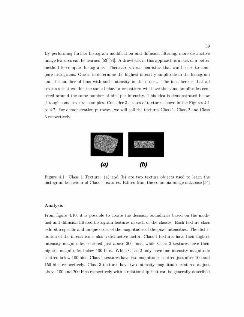
By performing further histogram modification and diffusion filtering, more distinctive
image features can be learned [53][54]. A drawback in this approach is a lack of a better
method to compare histograms. There are several heuristics that can be use to com-
pare histograms. One is to determine the highest intensity amplitude in the histogram
and the number of bins with such intensity in the object. The idea here is that all
textures that exhibit the same behavior or pattern will have the same amplitudes cen-
tered around the same number of bins per intensity. This idea is demonstrated below
through some texture examples. Consider 3 classes of textures shown in the Figures 4.1
to 4.7. For demonstration purposes, we will call the textures Class 1, Class 2 and Class
3 respectively.
Figure 4.1: Class 1 Texture: (a) and (b) are two texture objects used to learn thehistogram behaviour of Class 1 textures. Edited from the columbia image database [54]
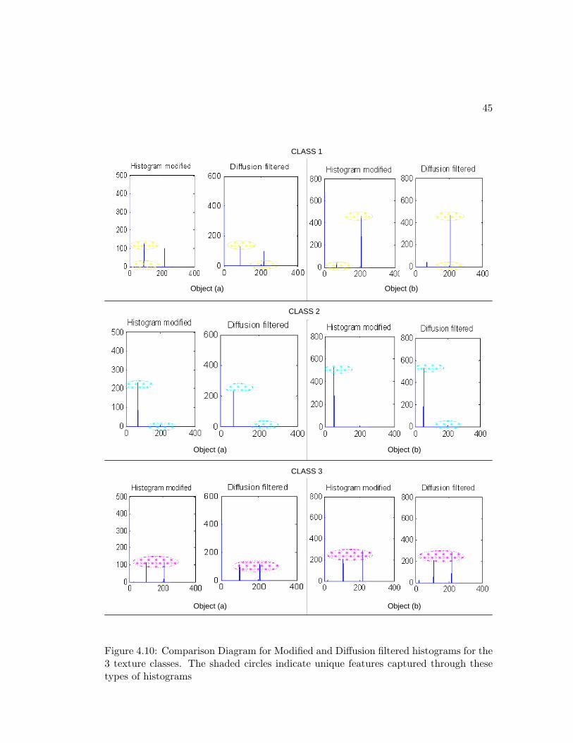
Analysis
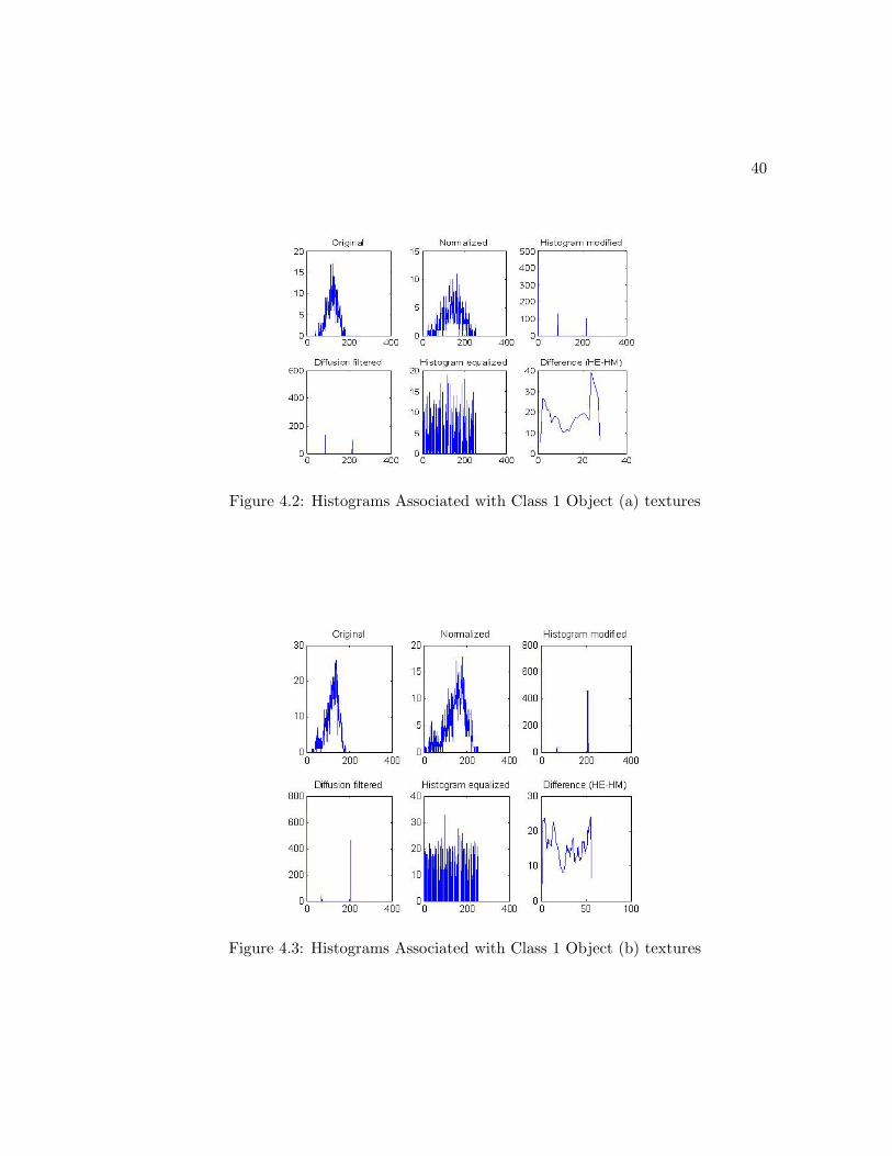
From figure 4.10, it is possible to create the decision boundaries based on the modi-
fied and diffusion filtered histogram features in each of the classes. Each texture class
exhibit a specific and unique order of the magnitudes of the pixel intensities. The distri-
bution of the intensities is also a distinctive factor. Class 1 textures have their highest
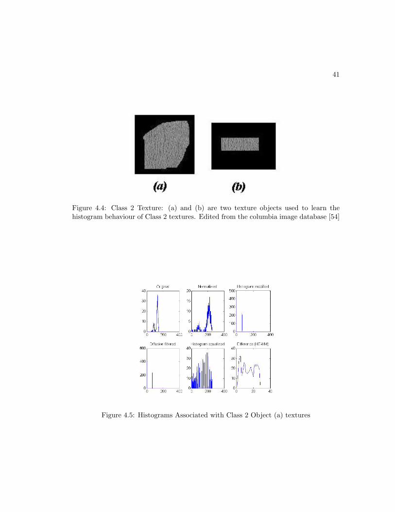
intensity magnitudes centered just above 200 bins, while Class 2 textures have their
highest magnitudes below 100 bins. While Class 2 only have one intensity magnitude
centred below 100 bins, Class 1 textures have two magnitudes centred just after 100 and
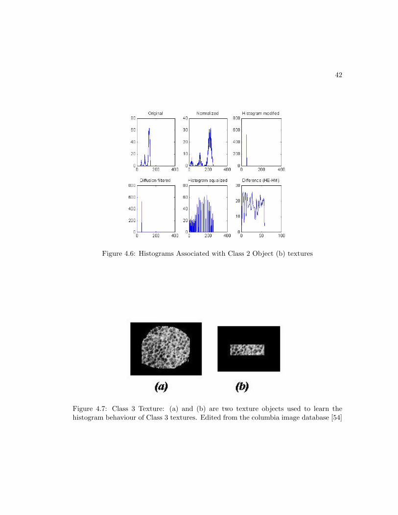
150 bins respectively. Class 3 textures have two intensity magnitudes centered at just
above 100 and 200 bins respectively with a relationship that can be generally described
40
Figure 4.2: Histograms Associated with Class 1 Object (a) textures
Figure 4.3: Histograms Associated with Class 1 Object (b) textures
41
Figure 4.4: Class 2 Texture: (a) and (b) are two texture objects used to learn thehistogram behaviour of Class 2 textures. Edited from the columbia image database [54]
Figure 4.5: Histograms Associated with Class 2 Object (a) textures
42
Figure 4.6: Histograms Associated with Class 2 Object (b) textures
Figure 4.7: Class 3 Texture: (a) and (b) are two texture objects used to learn thehistogram behaviour of Class 3 textures. Edited from the columbia image database [54]
43
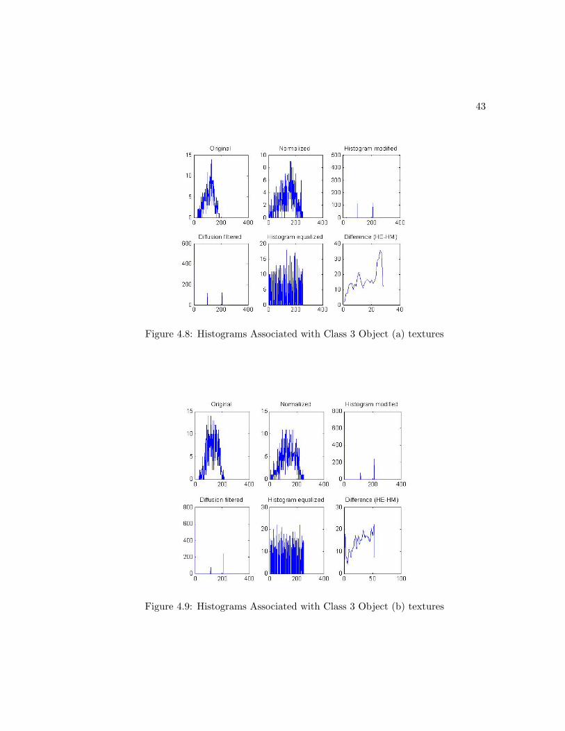
Figure 4.8: Histograms Associated with Class 3 Object (a) textures
Figure 4.9: Histograms Associated with Class 3 Object (b) textures
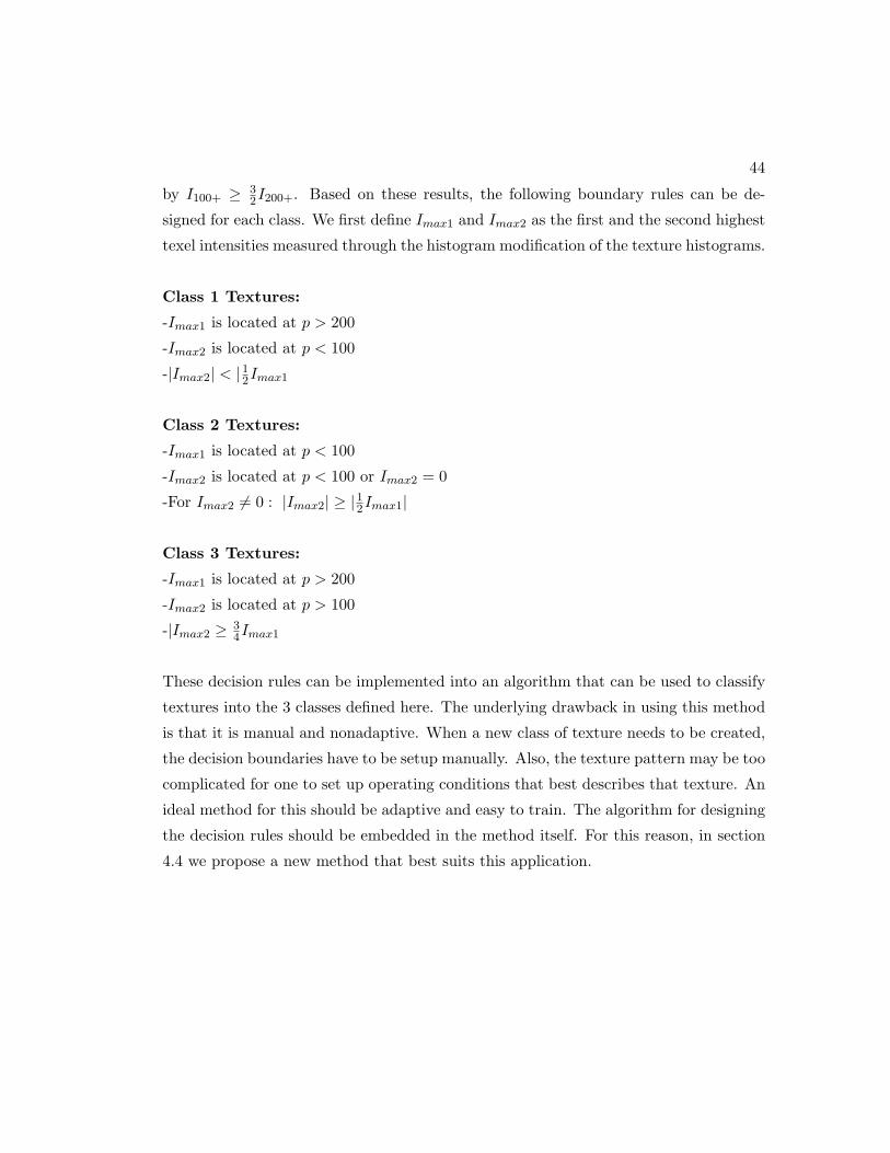
44
by I100+ ≥ 32I200+. Based on these results, the following boundary rules can be de-
signed for each class. We first define Imax1 and Imax2 as the first and the second highest
texel intensities measured through the histogram modification of the texture histograms.
Class 1 Textures:
-Imax1 is located at p > 200
-Imax2 is located at p < 100
-|Imax2| < |12Imax1
Class 2 Textures:
-Imax1 is located at p < 100
-Imax2 is located at p < 100 or Imax2 = 0
-For Imax2 6= 0 : |Imax2| ≥ |12Imax1|
Class 3 Textures:
-Imax1 is located at p > 200
-Imax2 is located at p > 100
-|Imax2 ≥ 34Imax1
These decision rules can be implemented into an algorithm that can be used to classify
textures into the 3 classes defined here. The underlying drawback in using this method
is that it is manual and nonadaptive. When a new class of texture needs to be created,
the decision boundaries have to be setup manually. Also, the texture pattern may be too
complicated for one to set up operating conditions that best describes that texture. An
ideal method for this should be adaptive and easy to train. The algorithm for designing
the decision rules should be embedded in the method itself. For this reason, in section
4.4 we propose a new method that best suits this application.
45
Object (a) Object (b)
Object (a) Object (b)
Object (a) Object (b)
CLASS 1
CLASS 2
CLASS 3
Figure 4.10: Comparison Diagram for Modified and Diffusion filtered histograms for the3 texture classes. The shaded circles indicate unique features captured through thesetypes of histograms
46
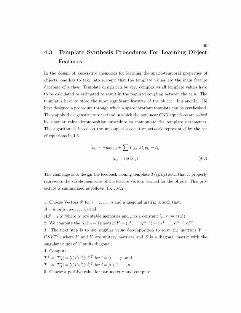
4.3 Template Synthesis Procedures For Learning Object
Features
In the design of associative memories for learning the spatio-temporal properties of
objects, one has to take into account that the template values are the main feature
database of a class. Template design can be very complex as all template values have
to be calculated or estimated to result in the required coupling between the cells. The
templates have to store the most significant features of the object. Liu and Lu [15]
have designed a procedure through which a space invariant template can be synthesised.
They apply the eigenstructure method in which the nonlinear CNN equations are solved
by singular value decomposition procedure to manipulate the template parameters.
The algorithm is based on the uncoupled associative network represented by the set
of equations in 4.6.
xij = −a00xij +∑
T (ij, kl)yij + Iij
yij = sat(xij) (4.6)
The challenge is to design the feedback cloning template T (ij, kj) such that it properly
represents the stable memories of the feature vectors learned for the object. This pro-
cedure is summarized as follows [15, 50-52]:
1. Choose Vectors βi for i = 1, . . . , n and a diagonal matrix A such that:
A = diag(a1, a2, . . . , ai) and,
Aβi = µαi where αi are stable memories and µ is a constant (µ ≥ max(a))
2. We compute the nx(m− 1) matrix Y = (y1, . . . , ym−1) = (α1, . . . , αm−1, αm)
3. The next step is to use singular value decomposition to solve the matrices Y =
USV T T , where U and V are unitary matrices and S is a diagonal matrix with the
singular values of Y on its diagonal.
4. Compute
T+ = [T+ij ] =
∑i(ui)(ui)T for i = 0, . . . , p, and
T− = [T−ij ] =∑
i(ui)(ui)T for i = p + 1, . . . , n
5. Choose a positive value for parameter τ and compute
47
T = µT+ + τT+ and I = µαm − Tαm
6. Then α1, ...., αm will be stored as memory vectors in the system 4.6.
This procedure yields a template T (ij, kl) which is symmetric and stable [15].
4.4 Feature Selection and Learning using Genetically Op-
timized CNNs
In this method, we propose the use of genetic algorithms to create stable memories that
store the features of the object. It is proposed that using the simplest CNN architecture,
the template parameters that best captures the features of the input can be estimated
through genetic algorithms. The method is based on optimising the parameters of the
kernel matrix (or cloning template) of the associative network described in chapter 2. In
practice, it may not be sufficient for the algorithm to be restricted into capturing certain
input traits modeled as deterministic rules or mathematical equations. An algorithm
that successfully selects the features without human intervention may yield better results
as there is no mathematical restrictions to govern the selection procedure. The selection
based on genetic algorithm tries to achieve this in practice.
4.4.1 Genetic Algorithms(GAs)
The main challenge that any optimization technique faces is termination at an optimal
solution that describes the global behavior of a process. During optimization, a poor
optimization method can get trapped in the local maxima, which may not be the best
solution in the solution space. This problem is common to most linear optimization
solutions.
Genetic Algorithms inherit their origins from the Darwinian theories of evolution [24,37,55-
59]. In this theory, the survival of a gene is a result of natural selection through fitness.
This natural process is achieved by applying certain genetic operators such as crossover
and mutation. Through these operators new genes that adapt to the competition en-
vironment are created, therefore getting rid of unfit genes that do not optimize the
solution.
Artificial GAs are based on stochastic sampling methods that increase the probability of
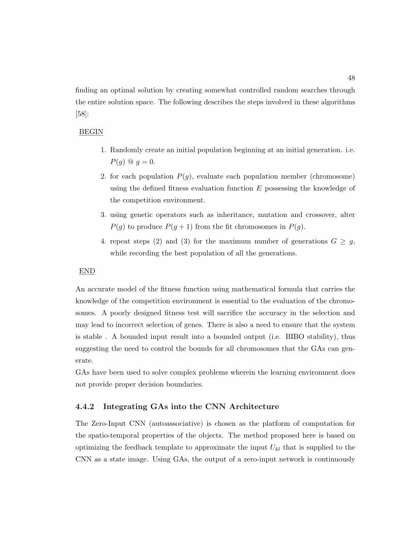
48
finding an optimal solution by creating somewhat controlled random searches through
the entire solution space. The following describes the steps involved in these algorithms
[58]:
BEGIN
1. Randomly create an initial population beginning at an initial generation. i.e.
P (g) @ g = 0.
2. for each population P (g), evaluate each population member (chromosome)
using the defined fitness evaluation function E possessing the knowledge of
the competition environment.
3. using genetic operators such as inheritance, mutation and crossover, alter
P (g) to produce P (g + 1) from the fit chromosomes in P (g).
4. repeat steps (2) and (3) for the maximum number of generations G ≥ g,
while recording the best population of all the generations.
END
An accurate model of the fitness function using mathematical formula that carries the
knowledge of the competition environment is essential to the evaluation of the chromo-
somes. A poorly designed fitness test will sacrifice the accuracy in the selection and
may lead to incorrect selection of genes. There is also a need to ensure that the system
is stable . A bounded input result into a bounded output (i.e. BIBO stability), thus
suggesting the need to control the bounds for all chromosomes that the GAs can gen-
erate.
GAs have been used to solve complex problems wherein the learning environment does
not provide proper decision boundaries.
4.4.2 Integrating GAs into the CNN Architecture
The Zero-Input CNN (autoassociative) is chosen as the platform of computation for
the spatio-temporal properties of the objects. The method proposed here is based on
optimizing the feedback template to approximate the input Ukl that is supplied to the
CNN as a state image. Using GAs, the output of a zero-input network is continuously
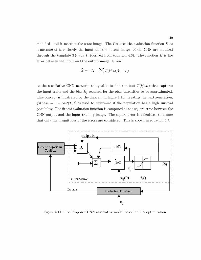
49
modified until it matches the state image. The GA uses the evaluation function E as
a measure of how closely the input and the output images of the CNN are matched
through the template T (i, j; k, l) (derived from equation 4.6). The function E is the
error between the input and the output image. Given:
X = −X +∑
T (ij, kl)Y + Iij
as the associative CNN network, the goal is to find the best T (ij; kl) that captures
the input traits and the bias Iij required for the pixel intensities to be approximated.
This concept is illustrated by the diagram in figure 4.11. Creating the next generation,
fitness = 1 − cost(T, I) is used to determine if the population has a high survival
possibility. The fitness evaluation function is computed as the square error between the
CNN output and the input training image. The square error is calculated to ensure
that only the magnitudes of the errors are considered. This is shown in equation 4.7:
Figure 4.11: The Proposed CNN associative model based on GA optimization
50
E = −∑
(Yij − Uij)2 (4.7)
where Yij is the output of the CNN and Uij is the training image (i.e. a small CNN
image containing details about the feature(s) characterizing a class). GA evaluation
technique is based on ensuring the highest value possible for the evaluation function
(i.e. finding chromosomes that maximise E). However, in this case it is required that
the smallest value possible be the optimal solution (i.e. reduced error). To ensure that
GA minimizes the error, error equation is negated such that the maximum possible
solution achievable in the network is zero.
With the CNN architecture adopted in this algorithm and a 3X3 template, the to-
tal number of parameters that need to be stored is 10, 9 of which represent a 3 X 3
convolution kernel Tij,kl and one represents the CNN bias Iij . It is well known that GA
performance decreases when searching in large parameter space as it becomes computa-
tionally challenging to iterate through all elements and observing their contribution to
the overall solution [38]. It thus becomes important to limit the number of parameters
that require optimization. Also, it has been reported in [38] that a CNN based on a
3X3 network has the ability to capture enough information on the training data.
The set of matrices in equation 4.8 represents a model of the chromosomes generated
by GAs and used to create a CNN kernel [62]:
T (i, j; k, l) =
seed(1) seed(2) seed(3)
seed(4) seed(5) seed(6)
seed(7) seed(8) seed(9)
,
Iij = seed(10) (4.8)
The GA solution bounds for the elements in matrices Tij,kl and Iij must be set in order
to have result in a bounded output (i.e. bounds [−x; +x] where −x and +x respectively
denotes the lowest and the highest chromosome values expected in the generations).
Chapter 5
The Analogic Algorithms for
Object Detection and
Classification in Multiple Object
Scenarios
This Chapter is the integration of all chapters that build up the basis of the proposed
algorithms. In this chapter, both the learning and classification methods based on the
discussions and propositions made in chapter 4 are developed. The main building blocks
of the learning and classification algorithms proposed in this case are the object extrac-
tion from a multiple object scene, feature extraction and learning; and the classification
of learned features into predefined classes. Two feature selection strategies for multiple
object scenes are proposed, namely (1) feature learning through GA optimization and
(2) texture learning through histograms.
The first method is based on designing autoassociative memories in the CNN model
and optimizing feature learning using GAs. This is achieved through the use of a zero-
input CNNs and genetically optimized, space-invariant cloning templates. For GAs to
efficiently optimize the kernel matrices of the CNN, the number of kernel parameters
51
52
that require GA modification should be small. The choice of the autonomous CNN net-
work facilitates the reduction of parameters in the kernel as the network only requires
the feedback template and the bias current to be set up. With the choice of a 3X3
network, the number of chromosomes required by the GA is reduced to 10.
The second approach that is proposed in this research is based on the comparisons
of the diffusion filtered(DF) and modified(MD) histograms generated for each object
texture. The shape and the locations of maximum intensities for different textures in
the DF and MD histograms are different. This information is used to design decision
boundaries for each texture class. A procedure for designing class boundaries by exam-
ining specific features in the histograms is proposed and outlined.
Firstly, this chapter introduces the spatio-temporal learning algorithm based on 3 stages,
namely the preprocessing stage that removes gaussian noise and enhance the image, the
object extraction technique that is based on boundary tracing and hole filling meth-
ods and the spatio-temporal learning of features in the object is done and the features
therein are grouped into categories or classes. As these parts have already been dis-
cussed in the chapters above, the discussions in this chapter will mainly be centered on
how they integrate to form a complete classification algorithm. Finally, the classification
algorithm proposed for this application is outlined.
5.1 Classification Using CNN Associative Memories and
GAs
5.1.1 The Extraction and Training Algorithms
An efficient algorithm for spatio-temporal learning is one that learns the most distin-
guishing features of the object from the environment in which the object appears in. If
the object appears in a different environment alone, the algorithm should possess the
knowledge to be able to detect the object. Taking this into account, the extraction
of the object in order to learn it separately from the environment becomes the first
step of the learning algorithm. The learning algorithm proposed here first implements
53
an analogic technique that filters out the noise and extract the object from a multiple
object environment before learning takes place. This is an important step as objects
in natural scenes do not often appear in the image alone. The extraction algorithm is
based on anisotropic diffusion and adaptive thresholding discussed in section 3.3.1 and
3.3.2 respectively. The second part of the algorithm is training the CNN associative
architecture for extraction and storage of input features as stable memories in cloning
templates. The training is implemented as a recursive genetic learning approach that
truncates the learning error towards an optimal solution (i.e globally stable memories).
This algorithm is summerised by the flow diagram in figure 5.1. The learning algorithm
can be described as follows:
1. For a 3X3 network, start off with a gene population of 10 and generation 1. -
estimate T (ij, kl) and I(ij) such that Y = U .
2. Evaluate the genes using the evaluation function E = Y − U where Y is the
output of the CNN and U is the training set. The smallest value of E indicates
the similarity between the input and the output, and thus the optimal stable
memories that must be stored in T (ij, kl) and I(ij)
3. The process must be repeated for a number of n generations, while the genetic
operators such as crossover and mutations are applied to yield the population for
the next generation.
4. A class is a set of template parameters that represent learned features of objects
with a similar behaviour (i.e. T (ij, kl) and I(ij) that are generated for each class).
Consider a multiple object image shown as an input of the learning algorithm in figure
5.2, the image is transformed for feature learning as shown by the optical flow in the
processing stages of the proposed algorithm.
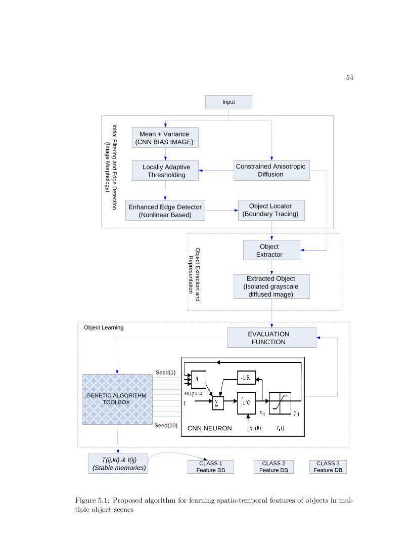
54
Input
CNN NEURON
GENETIC ALGORITHMTOOLBOX
EVALUATION FUNCTION
Mean + Variance(CNN BIAS IMAGE)
Constrained Anisotropic Diffusion
Locally Adaptive Thresholding
Enhanced Edge Detector(Nonlinear Based)
Object Locator(Boundary Tracing)
Object Extractor
Extracted Object(Isolated grayscale
diffused image)
Seed(1)
Seed(10)
T(ij,kl) & I(ij)(Stable memories)
Initial Filtering and Edge D
etection(Im
age Morphology)
Object E
xtraction and R
epresentation
Object Learning
CLASS 1Feature DB
CLASS 3Feature DB
CLASS 2Feature DB
Figure 5.1: Proposed algorithm for learning spatio-temporal features of objects in mul-tiple object scenes
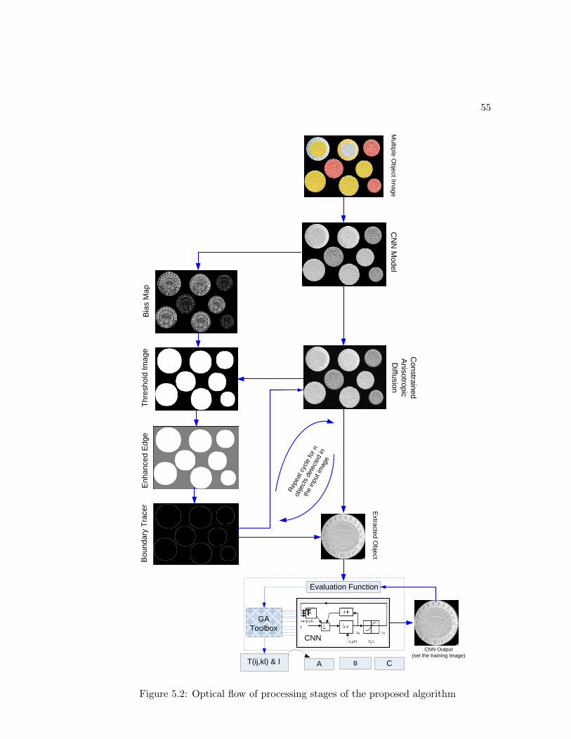
55
CN
N M
odel M
ultiple Object Im
age
Constrained
Anisotropic D
iffusion
Bia
s M
apTh
resh
old
Imag
eE
nhan
ced
Edge
Boun
dary
Tra
cer
A B C
GAToolbox
Evaluation Function
Repe
at c
ycle
for n
obje
cts
dete
cted
in
the
inpu
t im
age
T(ij,kl) & I
Extracted O
bject
CNNCNN Output
(set the training Image)
T
Figure 5.2: Optical flow of processing stages of the proposed algorithm
56
5.2 Texture-based Feature Extraction Using DF and MD
Histograms
The concept of using histograms to perform classification tasks was outlined in sec-
tion 4.2.2. Using diffusion filtered and modified histograms, different texel intensity
magnitudes in the object are detected. The number of bins with the highest texel in-
tensities in the histogram also represent how repetitive the texture pattern is. The
number of non-zero intensity magnitudes represent the unevenness of that texture and
the repetitiveness of each intensity. There are no established rules known in research for
comparing different histograms. In this section, various heuristics are used to formulate
a method for designing boundary conditions for each class based on the information
captured in the DF and MD histograms.
Using the CNN model, the training objects are extracted from a scene and enhanced
through CNN analogic algorithms for nonlinear diffusion and then MD and DF his-
tograms are generated. The histograms for each of the textures are then compared to
generate the decision boundaries that can be used to classify the textures. To generate
the decision boundaries, three highest texel intensities and their respective number of
bins are determined from the histograms and this information is compared for all ob-
jects in the same texture class. The bounds for the maximum intensities and number of
bins per area A of a certain texture are determined and the information is then stored
as class features.
Heuristics for Designing Texture-based Class Boundaries
From the illustrative DF histogram in Fig 5.3, we define:
-Imax3, Imax1 and Imax1 as the first, second and third highest intensities measured by
the histogram for a particular texture object. Imax3 > Imax2 > Imax1
-nbin is the number of bins with a particular texel intensity in the image per predefined
area A
-pos defines the bounds of an intensity magnitude in terms of number of bins
-nomax2 the boolean indicator for Imax2 measurements
57
-nomax1 the boolean indicator for Imax1 measurements
-n is a constant multiplier between texel intensities
-For A Class X texture shown in figure 5.3
• Imax2 > n ∗ Imax3. This condition determines the difference factor between the
highest and second highest intensities in the texture image.
• For Imax3: 0.75∗nbin < pos < nbin. The condition gives the bounds for number
of bins with highest maximum intensities in area A.
• For Imax2: 0.5∗nbin < pos < 0.75∗nbin. This condition is necessary to determine
the bounds for number of bins with Imax2 intensities
• If Imax2 == 0 : nomax2 = 0 else nomax2 = 1. This condition is necessary for
textures with only 1 non-zero intensity magnitudes.
• If Imax1 == 0 : nomax1 = 0 else nomax1 = 1. This condition is necessary for
textures with only 2 non-zero intensity magnitudes.
• Repeat these steps for other texture classes by studying the intensities and their
locations in the histograms and setting the parameters above accordingly.
The texture based feature learning approach outlined above is summerised in the flow
diagram shown in figure 5.4.
5.3 Classification Algorithm
The input of the classification is a multi-object scenario that has not been encountered
before. The entire image is passed into each class template for processing. The classi-
fication only require a constrained anisotropic diffusion filtering stage for noise removal
and enhancement of the image. An object belonging to Class A, for example, is only
visible if the template representing Class A features is applied, and so is for the rest of
the classes. Any object in the multiple object scene belonging to a class other than that
of the applied template is suppressed into a black background. The objects appear as a
set of white pixels distributed in the multiple object image. Colour coding can also be
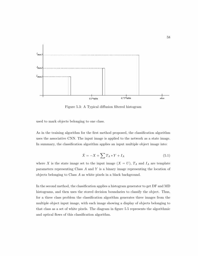
58
Figure 5.3: A Typical diffusion filtered histogram
used to mark objects belonging to one class.
As in the training algorithm for the first method proposed, the classification algorithm
uses the associative CNN. The input image is applied to the network as a state image.
In summary, the classification algorithm applies an input multiple object image into:
X = −X +∑
TA ∗ Y + IA (5.1)
where X is the state image set to the input image (X = U), TA and IA are template
parameters representing Class A and Y is a binary image representing the location of
objects belonging to Class A as white pixels in a black background.
In the second method, the classification applies a histogram generator to get DF and MD
histograms, and then uses the stored decision boundaries to classify the object. Thus,
for a three class problem the classification algorithm generates three images from the
multiple object input image, with each image showing a display of objects belonging to
that class as a set of white pixels. The diagram in figure 5.5 represents the algorithmic
and optical flows of this classification algorithm.
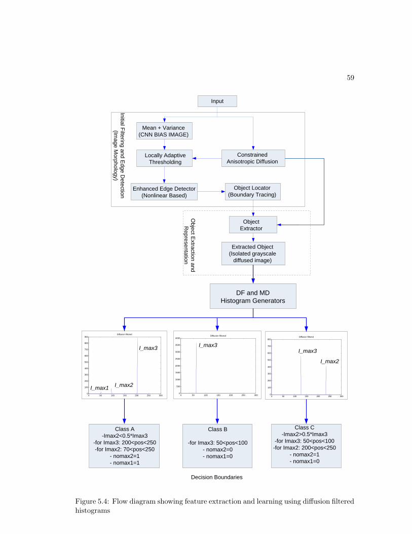
59
Input
Mean + Variance(CNN BIAS IMAGE)
Constrained Anisotropic Diffusion
Locally Adaptive Thresholding
Enhanced Edge Detector(Nonlinear Based)
Object Locator(Boundary Tracing)
Object Extractor
Extracted Object(Isolated grayscale
diffused image)
Initial Filtering and Edge D
etection(Im
age Morphology)
Object E
xtraction and R
epresentation
DF and MDHistogram Generators
0 50 100 150 200 250 3000
100
200
300
400
500
600
700
800
900Diffusion filtered
0 50 100 150 200 250 3000
500
1000
1500
2000
2500
3000
3500
4000Diffusion filtered
0 50 100 150 200 250 3000
100
200
300
400
500
600
700
800Diffusion filtered
I_max3
I_max2
I_max3I_max3
I_max2
Class A-Imax2<0.5*Imax3
-for Imax3: 200<pos<250-for Imax2: 70<pos<250
- nomax2=1- nomax1=1
Class B
-for Imax3: 50<pos<100- nomax2=0- nomax1=0
Class C-Imax2>0.5*Imax3
-for Imax3: 50<pos<100-for Imax2: 200<pos<250
- nomax2=1- nomax1=0
Decision Boundaries
I_max1
Figure 5.4: Flow diagram showing feature extraction and learning using diffusion filteredhistograms
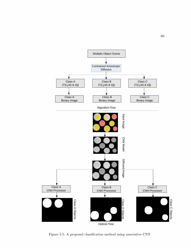
60
Multiple Object Scene
Class A(T(I,j,kl) & I(ij)
Class B(T(I,j,kl) & I(ij)
Class C(T(I,j,kl) & I(ij)
Contrained Anisotropic Diffusion
Class ABinary Image
Class BBinary Image
Class CBinary Image
Class ACNN Processor
Class BCNN Processor
Class CCNN Processor
Input Image
CN
N M
odelD
iffused Image
Class A
Objects
Class A
Objects
Class C
Objects
Algorithm Flow
Optical Flow
Figure 5.5: A proposed classification method using associative CNN
Chapter 6
Application Examples and
Analysis
In this chapter, application examples using the proposed algorithms are presented. The
first algorithm is applied to the field of satellite data modeling for landuse/cover classi-
fication purposes. In the resent past, there has been an increase in research for satellite
data interpretation. This is due to the increasing need to study the global phenom-
ena such as global warming, urbanization, climatic changes and land cover and land
use pattern changes. This is also yielded by the cheap availability of satellite data for
public use. Satellite sensing technologies have also improved significantly in the past,
now yielding satellite sensors with very high spatial, spectral and temporal resolutions.
Landsat have launched landsat 7 satellite that provides geographical data for the United
States Geographical Survey (USGS). The second algorithm is applied to a scene with
4-class texture objects. The Histogram modification is done and the decision bound-
aries for each class are established. The objects are then classified using the boundaries
formulated.
61
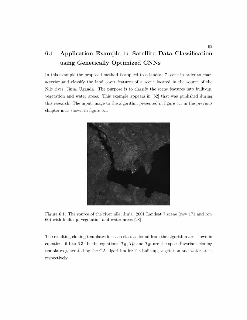
62
6.1 Application Example 1: Satellite Data Classification
using Genetically Optimized CNNs
In this example the proposed method is applied to a landsat 7 scene in order to char-
acterize and classify the land cover features of a scene located in the source of the
Nile river, Jinja, Uganda. The purpose is to classify the scene features into built-up,
vegetation and water areas. This example appears in [62] that was published during
this research. The input image to the algorithm presented in figure 5.1 in the previous
chapter is as shown in figure 6.1.
Figure 6.1: The source of the river nile, Jinja: 2001 Landsat 7 scene (row 171 and row60) with built-up, vegetation and water areas [28]
The resulting cloning templates for each class as found from the algorithm are shown in
equations 6.1 to 6.3. In the equations, TB, TV and TW are the space invariant cloning
templates generated by the GA algorithm for the built-up, vegetation and water areas
respectively.
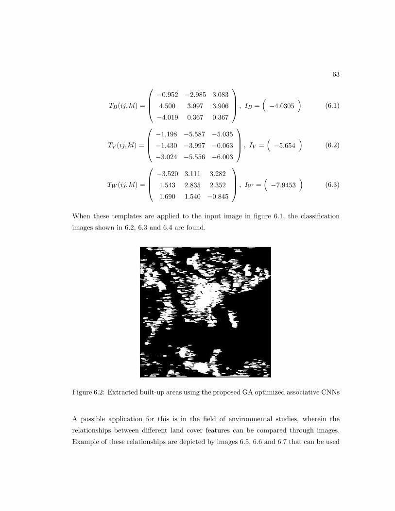
63
TB(ij, kl) =
−0.952 −2.985 3.083
4.500 3.997 3.906
−4.019 0.367 0.367
, IB =(−4.0305
)(6.1)
TV (ij, kl) =
−1.198 −5.587 −5.035
−1.430 −3.997 −0.063
−3.024 −5.556 −6.003
, IV =(−5.654
)(6.2)
TW (ij, kl) =
−3.520 3.111 3.282
1.543 2.835 2.352
1.690 1.540 −0.845
, IW =(−7.9453
)(6.3)
When these templates are applied to the input image in figure 6.1, the classification
images shown in 6.2, 6.3 and 6.4 are found.
Figure 6.2: Extracted built-up areas using the proposed GA optimized associative CNNs
A possible application for this is in the field of environmental studies, wherein the
relationships between different land cover features can be compared through images.
Example of these relationships are depicted by images 6.5, 6.6 and 6.7 that can be used
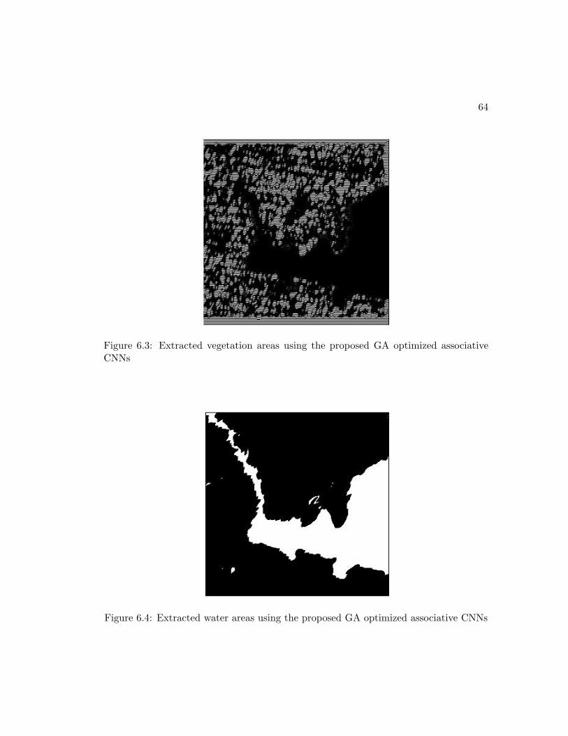
64
Figure 6.3: Extracted vegetation areas using the proposed GA optimized associativeCNNs
Figure 6.4: Extracted water areas using the proposed GA optimized associative CNNs
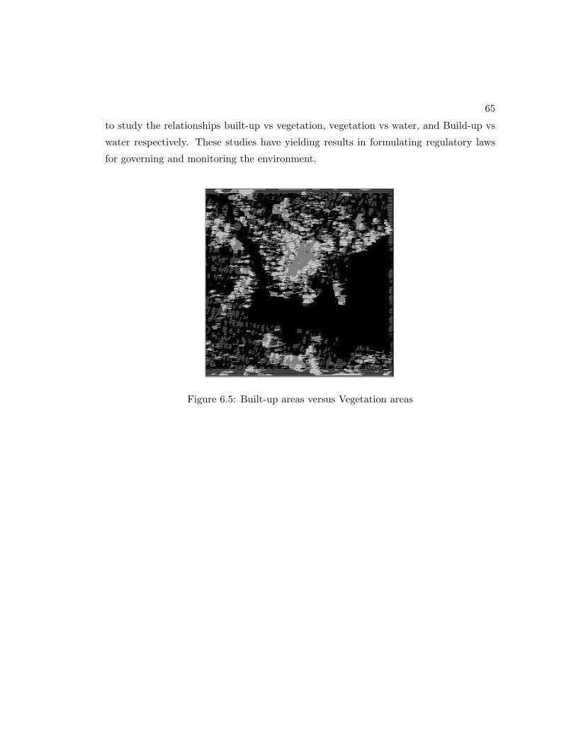
65
to study the relationships built-up vs vegetation, vegetation vs water, and Build-up vs
water respectively. These studies have yielding results in formulating regulatory laws
for governing and monitoring the environment.
Figure 6.5: Built-up areas versus Vegetation areas
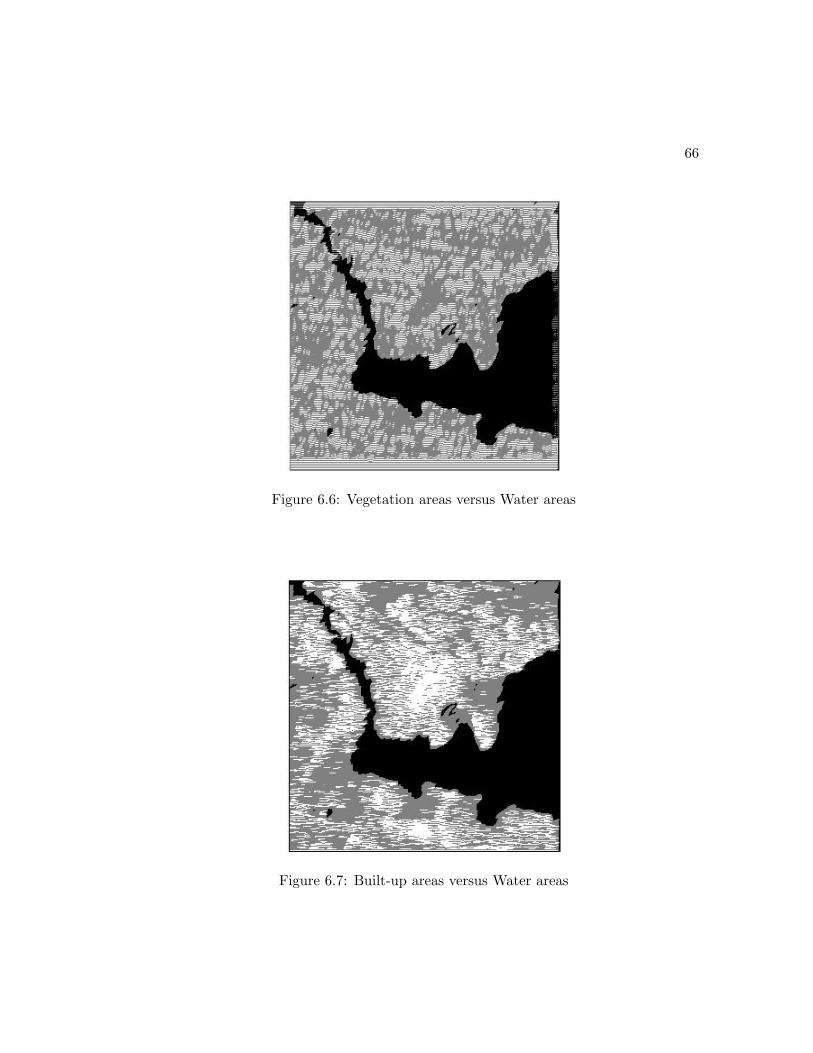
66
Figure 6.6: Vegetation areas versus Water areas
Figure 6.7: Built-up areas versus Water areas
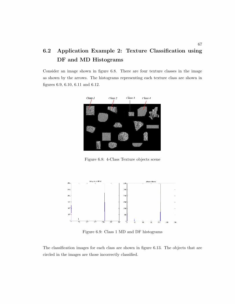
67
6.2 Application Example 2: Texture Classification using
DF and MD Histograms
Consider an image shown in figure 6.8. There are four texture classes in the image
as shown by the arrows. The histograms representing each texture class are shown in
figures 6.9, 6.10, 6.11 and 6.12.
Figure 6.8: 4-Class Texture objects scene
Figure 6.9: Class 1 MD and DF histograms
The classification images for each class are shown in figure 6.13. The objects that are
circled in the images are those incorrectly classified.
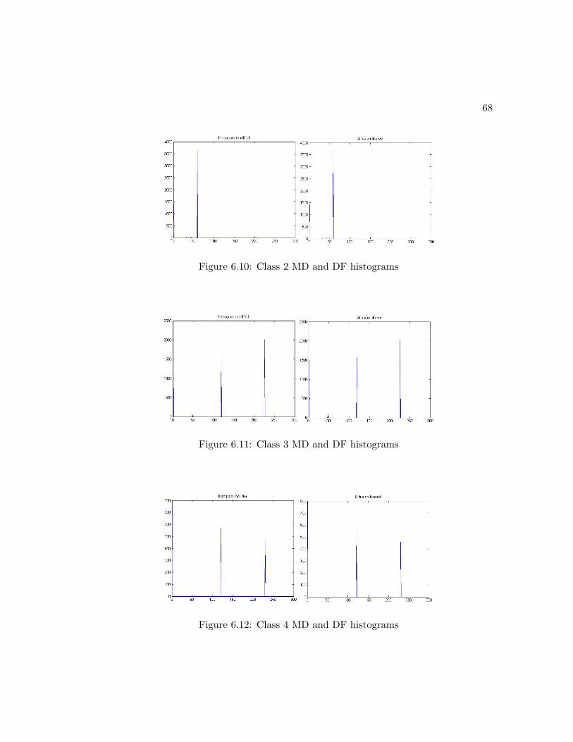
68
Figure 6.10: Class 2 MD and DF histograms
Figure 6.11: Class 3 MD and DF histograms
Figure 6.12: Class 4 MD and DF histograms
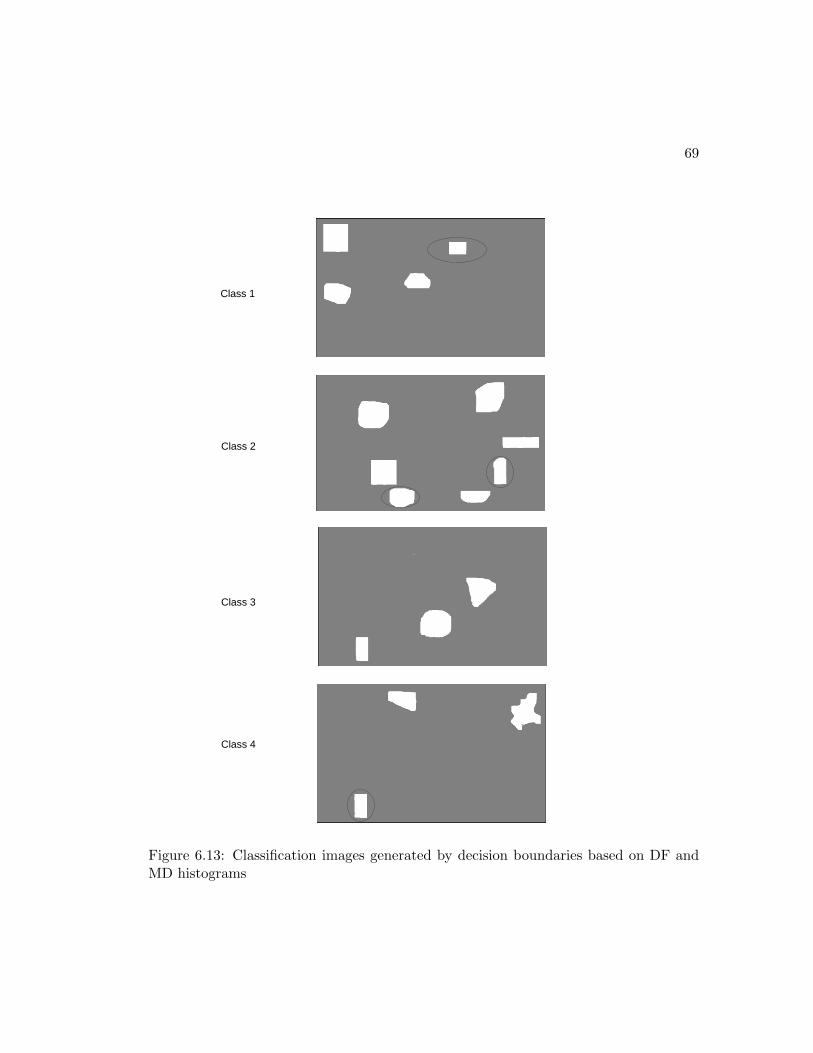
69
Class 1
Class 2
Class 3
Class 4
Figure 6.13: Classification images generated by decision boundaries based on DF andMD histograms
70
6.3 Analysis
Cellular Neural networks were introduced in Chapters 1 and 2 as a paradigm for com-
plexity. In this dissertation, a method of computing and understanding the spatio-
temporal properties of multiple object scenes was proposed, making use of CNNs as a
platform for computing. This chapter attempts to justify the suitability of CNNs for
spatio-temporal processing tasks through the analysis of the results from application
examples presented in sections 6.1 and 6.2. First the analysis procedure to be used is
presented, followed by the analysis of results from each example. The last section draws
the differences between CNN architectures and a well-known Hopfield network as a way
of demonstrating a number of advantages inherent in the use of the CNN the model in
spatio-temporal processing.
6.3.1 Analysis Procedure
In this section, the procedure to evaluate the performance of the solution proposed
for multiple object scenario is developed. The following aspects will be considered to
develop an analysis procedure:
• Architectural Efficiency - This test will measure the efficiency of the architec-
ture used in modeling the problem that this research has embarked to solve. The
aspects of architecture that are of concern are the simplicity of the model, integra-
tion suitability for on-chip spatio-temporal solutions, scalability and synchronous
processing.
• Memory efficiency and learning ability - This procedure will evaluate the
computational speed for both learning and classification algorithms.
• Processing Accuracy and Efficiency - Here the error rate of the proposed
solution is measured and the efficiency of the algorithm calculated based on the
application example presented in Chapter 6.
• Comparison with other network architectures - In this procedure the CNN
is compared with its counterparts based on established theories and limitations
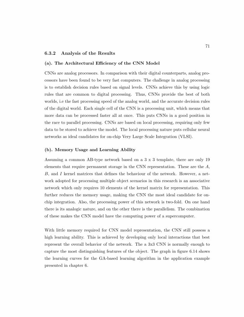
71
6.3.2 Analysis of the Results
(a). The Architectural Efficiency of the CNN Model
CNNs are analog processors. In comparison with their digital counterparts, analog pro-
cessors have been found to be very fast computers. The challenge in analog processing
is to establish decision rules based on signal levels. CNNs achieve this by using logic
rules that are common to digital processing. Thus, CNNs provide the best of both
worlds, i.e the fast processing speed of the analog world, and the accurate decision rules
of the digital world. Each single cell of the CNN is a processing unit, which means that
more data can be processed faster all at once. This puts CNNs in a good position in
the race to parallel processing. CNNs are based on local processing, requiring only few
data to be stored to achieve the model. The local processing nature puts cellular neural
networks as ideal candidates for on-chip Very Large Scale Integration (VLSI).
(b). Memory Usage and Learning Ability
Assuming a common AB-type network based on a 3 x 3 template, there are only 19
elements that require permanent storage in the CNN representation. These are the A,
B, and I kernel matrices that defines the behaviour of the network. However, a net-
work adopted for processing multiple object scenarios in this research is an associative
network which only requires 10 elements of the kernel matrix for representation. This
further reduces the memory usage, making the CNN the most ideal candidate for on-
chip integration. Also, the processing power of this network is two-fold. On one hand
there is its analogic nature, and on the other there is the parallelism. The combination
of these makes the CNN model have the computing power of a supercomputer.
With little memory required for CNN model representation, the CNN still possess a
high learning ability. This is achieved by developing only local interactions that best
represent the overall behavior of the network. The a 3x3 CNN is normally enough to
capture the most distinguishing features of the object. The graph in figure 6.14 shows
the learning curves for the GA-based learning algorithm in the application example
presented in chapter 6.
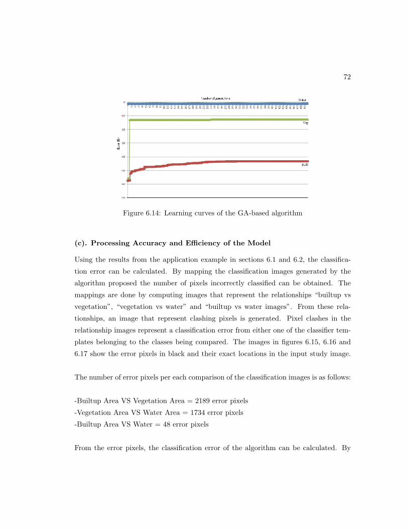
72
Figure 6.14: Learning curves of the GA-based algorithm
(c). Processing Accuracy and Efficiency of the Model
Using the results from the application example in sections 6.1 and 6.2, the classifica-
tion error can be calculated. By mapping the classification images generated by the
algorithm proposed the number of pixels incorrectly classified can be obtained. The
mappings are done by computing images that represent the relationships “builtup vs
vegetation”, “vegetation vs water” and “builtup vs water images”. From these rela-
tionships, an image that represent clashing pixels is generated. Pixel clashes in the
relationship images represent a classification error from either one of the classifier tem-
plates belonging to the classes being compared. The images in figures 6.15, 6.16 and
6.17 show the error pixels in black and their exact locations in the input study image.
The number of error pixels per each comparison of the classification images is as follows:
-Builtup Area VS Vegetation Area = 2189 error pixels
-Vegetation Area VS Water Area = 1734 error pixels
-Builtup Area VS Water = 48 error pixels
From the error pixels, the classification error of the algorithm can be calculated. By
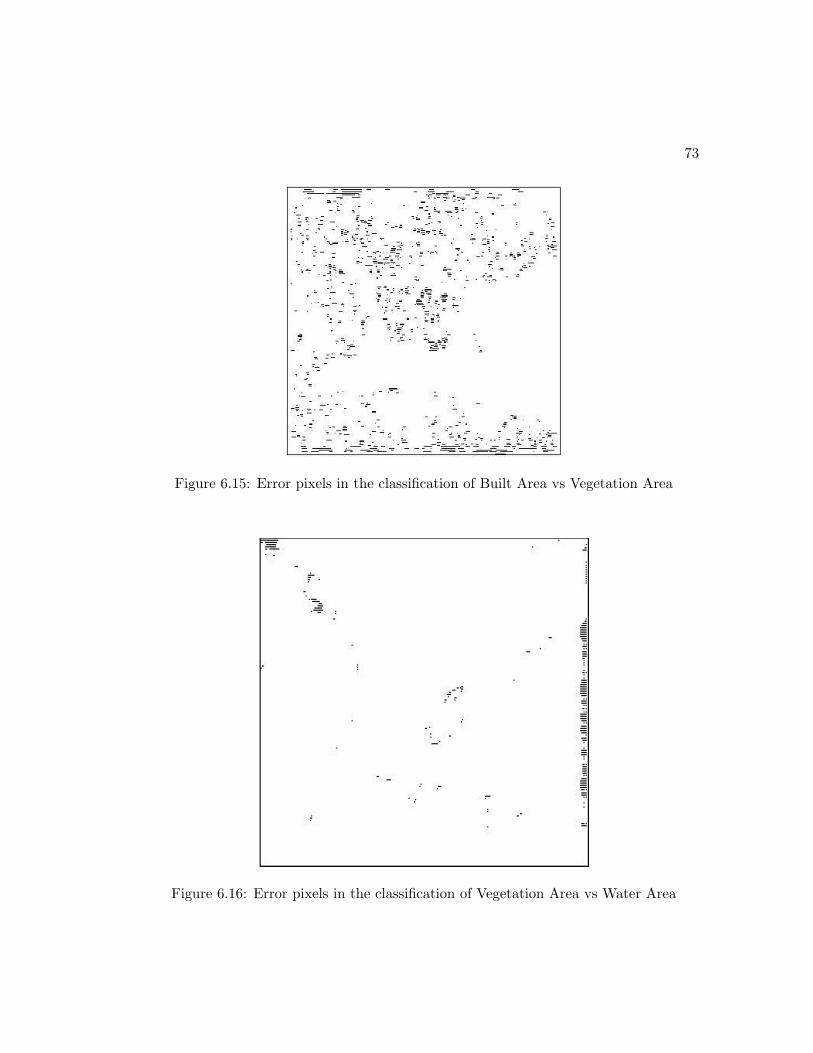
73
Figure 6.15: Error pixels in the classification of Built Area vs Vegetation Area
Figure 6.16: Error pixels in the classification of Vegetation Area vs Water Area
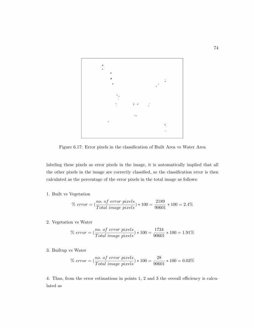
74
Figure 6.17: Error pixels in the classification of Built Area vs Water Area
labeling these pixels as error pixels in the image, it is automatically implied that all
the other pixels in the image are correctly classified, so the classification error is then
calculated as the percentage of the error pixels in the total image as follows:
1. Built vs Vegetation
% error = (no. of error pixels
Total image pixels) ∗ 100 =
218990601
∗ 100 = 2.4%
2. Vegetation vs Water
% error = (no. of error pixels
Total image pixels) ∗ 100 =
173490601
∗ 100 = 1.91%
3. Builtup vs Water
% error = (no. of error pixels
Total image pixels) ∗ 100 =
2890601
∗ 100 = 0.03%
4. Thus, from the error estimations in points 1, 2 and 3 the overall efficiency is calcu-
lated as
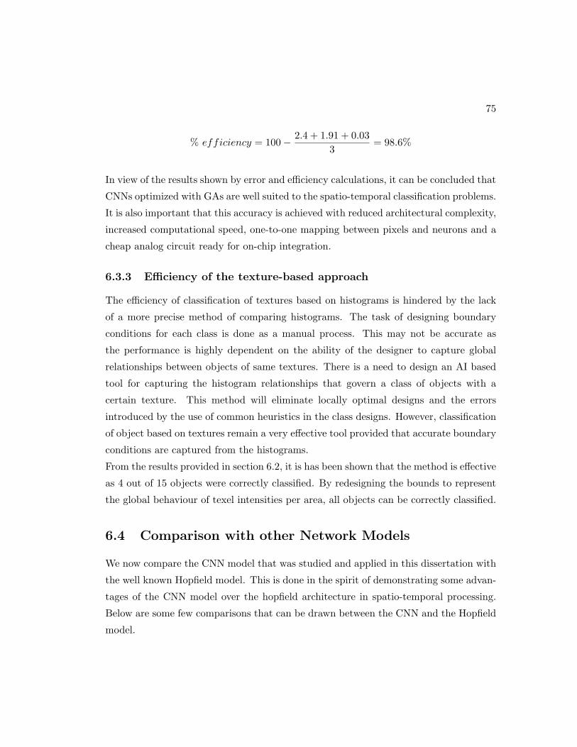
75
% efficiency = 100− 2.4 + 1.91 + 0.033
= 98.6%
In view of the results shown by error and efficiency calculations, it can be concluded that
CNNs optimized with GAs are well suited to the spatio-temporal classification problems.
It is also important that this accuracy is achieved with reduced architectural complexity,
increased computational speed, one-to-one mapping between pixels and neurons and a
cheap analog circuit ready for on-chip integration.
6.3.3 Efficiency of the texture-based approach
The efficiency of classification of textures based on histograms is hindered by the lack
of a more precise method of comparing histograms. The task of designing boundary
conditions for each class is done as a manual process. This may not be accurate as
the performance is highly dependent on the ability of the designer to capture global
relationships between objects of same textures. There is a need to design an AI based
tool for capturing the histogram relationships that govern a class of objects with a
certain texture. This method will eliminate locally optimal designs and the errors
introduced by the use of common heuristics in the class designs. However, classification
of object based on textures remain a very effective tool provided that accurate boundary
conditions are captured from the histograms.
From the results provided in section 6.2, it is has been shown that the method is effective
as 4 out of 15 objects were correctly classified. By redesigning the bounds to represent
the global behaviour of texel intensities per area, all objects can be correctly classified.
6.4 Comparison with other Network Models
We now compare the CNN model that was studied and applied in this dissertation with
the well known Hopfield model. This is done in the spirit of demonstrating some advan-
tages of the CNN model over the hopfield architecture in spatio-temporal processing.
Below are some few comparisons that can be drawn between the CNN and the Hopfield
model.
76
Table 6.1: Comparison of the CNN and the Hopfield Models.
Area CNN Hopfield
Network Connectiv-
ity
Local Global
Operating mode Synchronous mode Asynchronous
Associative Memo-
ries
Coupling rules set by tem-
plate synthesis procedures or
Optimization
Weights are computed by the
Hebb rule
Processing Circuitry Analog circuit Digital Circuit
Processing Elements Cells Nodes
Spatio-temporal
Mapping
One-to-one with image pixels Depends on representation
Number of Inputs vs
Network Nodes
A CNN of n = NXM =
9 for M = N = 3, r = 3 has
a total of 289 interconnections
A Hopfield Network of n = 9
has a total of 729 interconnec-
tions
Template symmetry No assumption about tem-
plate symmetry
Template is required to be
symmetric
Chapter 7
Conclusion, Discussions and
Recommendations
7.1 On Suitability of the CNN to Spatio-temporal Pro-
cessing
Using the CNN model, it has been illustrated in this dissertation that a complex system
can be modeled using an associative network. The model only requires few elements and
is mathematically easy. Through achieving the model of a cell that best represent the
data structure and its patterns in the network, a complex environment is reduced into
a model easy to understand and compute. In this dissertation, we chose autonomous
CNNs as the platform for modeling the spatio-temporal properties of objects. The model
has led to a proper extraction of the objects and the ease of formulation for learning
methods. An accuracy of 98% in the classification problem outlined in section 6 indicates
that these networks have high performance in spatio-temporal environments. There is
also a notable difference in structural constituents between the CNNs and the Hopfield
as tabulated in Table 6.1 of section 6. This has yielding factors in terms of computa-
tional speed, memory usage and implementation difficulties. These further motivates
the adoption of CNNs by many researchers as an image processing platform. Through
this research, the powerful processing nature of the CNN has been demonstrated.
77
78
7.2 On Feature Learning and Classification
Like any other network, the CNN performance in classification also require further opti-
mization to terminate at a global solution for each class of objects. This document has
proposed the use of Genetic Algorithms to optimize autoassociative CNNs to perform
learning of spatio-temporal features. It is important to note that most of the feature
learning algorithms known in research are instructed by a user program to capture
certain specific features (measured through mathematical computations) of the object.
The proposed algorithm using GAs in this research does not make this assumption. It
however allows the learning algorithm to extract any feature(s) from the object that
best distinguish it from the rest. This presents an advantage in cases where there may
not be a better mathematical model for extracting features. We single out one statisti-
cal feature extractor that is worth noting, this is the texture histograms. Though this
method requires a lot of manual computations in forming decision boundaries for object
classes, it remains effective. With accurate class design all the objects in a multiple
object scene can be correctly classified.
The efficiency of the CNN network also lies in the ability to implement analogic algo-
rithms. This means that certain templates required in more than one processing stages
can be reused whenever the need arise. These analogic algorithms take place at pixel
level and hence are applied in accordance with the required or existing coupling rules
on the network. This very nature of CNNs makes them more easier to design and scale
according to the application requirements.
7.3 Research Contribution
This section serves as a reaffirmation of the contributions stated in section 1.4. The
algorithms developed on chapters 4 and 5 yield a solution which reduces model com-
plexity, increases the computational speed as well as the easy-to-implement training
algorithm for samples to be detected. This document has outlined various advantages
of CNNs over classic image processing methods. Also, this research work has also ad-
dressed a solution of modeling with multiple image scenes. By learning each object from
its surrounding environment (i.e. in a multiple image scene of its existence), the object
appearing in a multiple image scene can be easily detected and classified. The solutions
79
proposed in this research are applicable to industrial processing tasks such as visual
quality inspection, surveillance and monitoring as well as geographical data analysis.
This research proposes an efficient way of handling scenes with more than one object
belonging to different classes.
7.4 Future Work and Recommendations
Though the algorithm proposed in this dissertation was reported to be efficient, there
are areas of concern that require further research. The accuracy of Genetic Algorithms
has shown a decrease when the need to use templates with neighbourhoods greater than
2 arise. While templates with more parameters may capture more data on the input,
they cannot be optimized using GAs unless the parameters are reduced by setting some
to constant values. Setting some parameters to constant values may sacrifice the tem-
plate’s feature capturing abilities, while leaving them as variables for GA optimization
may result in a large GA solution space that may not terminate at optimal templates.
Arriving at a trade-off between these two is a matter of further research.
There is also the need to devise a standardized method for histogram comparisons in
texture-based feature extractions. Histograms provide more important aspects about
textures on the image, thus a better way of establishing texture classes will be in support
of the strength of histograms in this field.
References
[1] L. Fortuna, P. Arena, D. Balya and A. Zarandy, “Cellular Neural Networks: A
Paradigm for Nonlinear Spatio-temporal Processing”, Circuits and Systems Magazine,
IEEE, Vol. 1, Issue: 4, 2001, pp. 6-21.
[2] O. V. de Paul, “Remote Sensing: New Applications for Urban Areas”, Proceed-
ings of the IEEE, Dec. 2007, Volume 95, Issue 12, pp. 2267 - 2268.
[3] M. H. ter Brugge, R. J. Krol, J. A. G. Nijhuis, L. Spaanenburg, “Design of Discrete-
Time Cellular Neural Networks Based on Mathematical Morphology”, Proceedings of the
fourth IEEE International Workshop on Cellular Neural Networks (CNNA-96), Seville
(Spain), June 1996, pp. 1-5.
[4] L. Spaanenburg et al, “Natural learning of neural networks by reconfiguration”,
Proc. SPIE, Bioengineered and Bioinspired Systems, Vol. 5119, April 2004, pp. 273-
284
[5] L. O. Chua and L. Yang, “Cellular Neural Networks: Theory”, IEEE Trans. On
Circuits and Systems, Vol. 35, No. 10, October 1988, pp. 1257-1272.
[6] L. O. Chua. “CNN: A Paradigm for Complexity”,World Scientific Series on Non-
linear Science,Vol 1, Series A, June 1998.
80
81
[7] L. M. Lederman and D. N. Schramm, “From Quarks to the Cosmos: Tools of Dis-
covery”, volume 28 of Scientific American Library Series. W.H. Freeman and Company,
1995. [8] L.O. Chua and T. Roska, Cellular Neural Networks Paradigm, IEEE Trans.
on Circuits and Systems I: Fundamental Theory and Applications, Vol. 40, No. 3, Mar
1993, pp. 147-156.
[9] S. Xavier-de-Souza, J. A. K. Suykens, and J. Vandewalle. “Learning of Spatiotem-
poral Behavior in Cellular Neural Networks”. International Journal of Circuit Theory
and Applications - Special Issue on CNN Technology (Part 1), 34:127140, Jan 2006.
[10] L.O. Chua and T. Roska, Cellular neural networks and visual computing, Foun-
dations and applications (Cambridge UK: Cambridge University Press, 2002) 205-231.
[11] M. G. Milanova, A. Elmaghraby, S. Rubin, “Cellular Neural Networks for Seg-
mentation of Image Sequence”, Journal on Neurocomputing, Vol. 31(1-4), 2000, pp.
125-141.
[12] W. Aziz and T. Lala, “Controllability, Applications, and Numerical Simulations
of Cellular Neural Networks”, 2003 Colloquium on Differential Equations and Applica-
tions, Maracaibo, Venezuela. Electronic Journal of Differential Equations, Conference
13, 2005, pp. 111.
[13] J. Austin, “The cellular neural network associative processor, C-NNAP”, Fifth
International Conference on Image Processing and its Applications, 1995, pp. 622-626.
[14] P. Szolgay, I. Szatmari, and K. Laszlo, “A Fast Fixed Point Learning Method
to Implement Associative Memory on CNNs”, Circuits and Systems I: Fundamental
Theory and Applications, IEEE Transactions on Circuits and Systems I, Vol. 44, Issue
4, Apr 1997, pp. 362-366.
82
[15] Z. Lu and D. Liu, A New Synthesis Procedure for a Class of Cellular Neural Net-
works with Space-Invariant Cloning Template, IEEE Trans. on Circuits and Systems
IIAnalog and Digital Signal Processing, Vol. 45, No. 12, December 1998.
[16] T. Roska, K. Lotz, J. Hamori, E. Labos, and J. Takacs, “The CNN model in
the visual system”, Part 1: The CNN-retina and some direction and length-selective
mechanisms, Research Report of the Analogic (Dual) and Neural Computing Systems
Laboratory (DNS-8-1991), Budapest, MTA SZTAKI.
[17] J.L. Teeters F.S. Weblin, “Real-time simulation of retina allowing visualization
of each processing stage”,SPIE, 1472. [18] T. Roska, “Cellular Wave Computers for
Brain-like Spatial-temporal Sensory Computing”, IEEE ISCAS 2004 Plenary Lecture,
Vancouver, May, 2004.
[19] Y. Wang, W. Zhou and X. Wang, “Cellular Neural Networks for Object Segmenta-
tion of Image Sequence”, Asian Journal of Information Technology , Vol. 4(11), 2005,
pp. 1098-1101.
[20] T. Szabo and P. Szolgay, “Analogic Diffusion-Based Algorithm for the segmenta-
tion of CT/MRI Images”,Circuit Theory and Design. Proceedings of the 16th European
Conference ECCTD’03, Vol. 1, 2003, pp. 237-239.
[21] C. Rekeczky, “Adaptive Multi-rate, Multi-grid and Multi-scale Algorithms Run-
ning on Analogic Architecture”,Circuit Theory and Design. Proceedings of the 16th
European Conference ECCTD’03. Vol. 1, 2003, pp. 404-404.
[22] D. Balya, T. Gergely, I. Szatmari, and C. Rekeczky, “Classification of Spatio-
Temporal Features: The Nearest Neighbor Family”, The 16th European Conference on
Circuits Theory and Design, ECCTD’03, Vol. 3, 2003, pp. 129-132.
[23] D. Balya, G. Timar, I. Szatmari, and Cs. Rekeczky, “Efficient Off-line Feature
83
Selection Strategies for On-line Classifier Systems”, in Proc. of the IEEE Int. Joint
Conference IJCNN’04, Vol. 1, 2004, pp. 171-176.
[24] F. Dellaert and J. Vandewalle, “Automatic Design of Cellular Neural Networks
by means of Genetic Algorithms: Finding a Feature Detector”, in Proc. IEEE Int.
Workshop on Cellular Neural Networks and Their Applications, 1994, pp. 189-194.
[25] O. Dekhtyarenko, A. Reznik and A. Sitchov, “Associative Cellular Neural Net-
works with Adaptive Architecture”, In proc. of The 8th IEEE International Biannual
Workshop on Cellular Neural Networks and their Application (CNNA’04), Budapest,
Hungary, July 2004, pp. 219-224.
[26] C. K. I. Williams and M. K. Titsias. “Learning about multiple objects in images:
Factorial learning without factorial search”. Advances in Neural Information Processing
Systems,2003, pp. 1415-1422.
[27] Williams, C. K. I. and Titsias, M. T. (2003). Learning about multiple objects
in images:Factorial learning without factorial search. In Becker, S., Thrun, S., and
Obermayer, K., editors, Advances in Neural Information Processing Systems. MIT
Press.
[28] R. Simmon, “NASA image based on Landsat-7 data provided by the UMD Global
Land Cover Facility”. U.S Geological Survey, Internet Listing, Last accessed: 17 De-
cember 2008, Last updated: 22 Sep 2008,
http://earthobservatory.nasa.gov/IOTD/
[29] A. Schultz, C. Rekeczky, I. Szatmri, T. Roska, and L.O. Chua, “Spatio-temporal
CNN Algorithm for Object Segmentation and Object Recognition”, 5th IEEE Int.
Workshop on Cellular Neural Networks and their Applications (CNNA-98), pp. 347-
352, London, April 14-19, 1998.
84
[30] C. Rekeczky, “Analogic CNN Simulation Toolbox for MATLAB”, Analogical and
Neural Computing Laboratory,Computer and Automation Institute, Hungarian Academy
of Sciences,H-1111 Budapest, Kende u. 13-17.
[31] T. Boros, K. Lotz, A. Radvnyi, and T. Roska, Some Useful New Nonlinear and
Delay-type Templates, Research report of the Analogical and Neural Computing Labo-
ratory, Computer and Automation Research Institute, Hungarian Academy of Sciences
(MTA SzTAKI), DNS-1-1991, Budapest, 1991.
[32] H. Harrer, P. L. Venetianer, J. A. Nossek, T. Roska, and L. O. Chua, “Some Ex-
amples of Preprocessing Analog Images with Discrete-Time Cellular Neural Networks”,
Proceedings of the International Workshop on Cellular Neural Networks and their Ap-
plications (CNNA-94), pp. 201-206, Rome, 1994.
[33] J. Weickert,“Anisotropic diffusion in image processing”, ECMI Series, Teubner,
Stuttgart, 1998. ISBN 3-519-02606-6.
[34] P. Perona and J.Malik, “Scale-Space and Edge Detection Using Anisotropic Diffu-
sion”, IEEE Trans.on PAMI, Vol. 12, July 1990, pp. 629-639.
[35] D. Keysers and C. H. Lampert and T. M. Breuel, “Color image dequantization
by Constrained Diffusion”,SPIE Electronic Imaging, 2006.
[36] J. Weickert, Applications of Nonlinear Diffusion In Image Processing and Com-
puter Vision, Proceedings of Algoritmy 2000. Acta Math., Univ. Comenianae Vol.
LXX, 1(2001), pp. 3350.
[37] M. J. Black, G. Sapiro, D. H. Marimont,and D. Heeger, “Robust Anisotropic Dif-
fusion”, IEEE Trans on Image Processing, VOL. 7, NO. 3, MARCH 1998.
[38] T. Sziranyi and M. Csapodi, Texture Classification and Segmentation by Cellular
85
Neural Networks Using Genetic Learning, Computer Vision and Image Understanding,
Vol. 71, No. 3, September 1998, pp. 255-270.
[39] Cs. Rekeczky, T. Roska, and A. Ushida, “CNN-based Difference-Controlled Adap-
tive Nonlinear Image Filters”, International Journal of Circuit Theory ans Applications,
Vol 26,1998, pp 375-423.
[40] L. Nemes, L. O. Chua, and T. Roska, “Implementation of Arbitrary Boolean Func-
tions on the CNN Universal Machine”, International Journal of Circuit Theory ans
Applications, Vol 26 (6), 1998,pp 593-610.
[41] T. Roska, L. Kk, L. Nemes, and . Zarndy (ed),“CNN Software Library (Templates
and Algorithms) Version 7.0”, Research report of the Analogic (Dual) and Neural Com-
puting Systems Laboratory, (DNS-1-1997), Budapest MTA SZTAKI, 1997.
[42] M. Gilli, “Template Design Methodologies and Tools”, European Conference on Cir-
cuit Theory and Design - ECCTD’99, Design Automation Day proceedings, (ECCTD’99-
DAD), pp. 113-126, Stresa, Italy, 1999.
[43] . Zarndy, “The Art of CNN Template Design”, Int. J. Circuit Theory and Appli-
cations - Special Issue: Theory, Design and Applications of Cellular Neural Networks:
Part II: Deign and Applications, (CTA Special Issue - II), Vol.17, No.1, pp.5-24, guest
ed: T. Roska, A. Rodriguez-Vazquez and J. Vandewalle, 1999,
[44] B. Mirzai, D. Lim, G.S. Moschytz, “Robust CNN Templates: Theory and Sim-
ulations”, Proceedings of IEEE Int. Workshop on Cellular Neural Networks and Their
Applications, (CNNA’96), pp.393-398, Sevilla, 1996,
[45] K. R. Crounse and L. O. Chua, “Methods for image processing and pattern forma-
tion in cnn:A tutorial.” 42, no. 10, (1995),pp 583601.
86
[46] Leon O. Chua and L. Yang, “Cellular neural networks: Applications”, IEEE.
Transc. Circuits Syst. 35 (1988),pp 12731290.
[47] P. Liu, N. Wu, J. Zhu, J. Yin, and W. Zhang, “A Unified Strategy of Feature
Selection”,Lecture Notes in Computer Science, Advanced Data Mining and Applica-
tions, Vol 4093, July 2006, pp. 457-464.
[48] M. Tuceryan and A. K. Jain, “Texture Analysis”,The Handbook of Pattern Recog-
nition and Computer Vision (2nd Edition), Chapter 2.1, pp. 207-248, World Scientific
Publishing Co., 1998.
[49] B. E. Shi and K. Boahen, “Competitively Coupled Orientation Selective Cellu-
lar Neural Networks”, IEEE Trans. On Circuits and SystemsI: Fundamenta Theory
and Applications, VOL. 49, NO. 3, MARCH 2002.
[50] D. Liu and A. N. Michel, “Dynamical Systems with Saturation Nonlinearities:
Analysis and Design”, New York: Springer-Verlag, 1994.
[51] D. Liu and A. N. Michel, “Sparsely interconnected neural networks for associa-
tive memories with applications to cellular neural networks”, IEEE Trans. Circuits
Syst. II, vol. 41, pp. 295309, Apr. 1994
[52] D. Liu and A. N. Michel, “Robustness analysis and design of a class of neural
networks with sparse interconnecting structure”, Neurocomputing, vol. 12, pp. 5976,
June 1996.
[53] R. A. Hummel, “Histogram Modification Techniques”, Computer Graphics and
Image Processing, vol. 4, 1975, pp.209-224.
[54] K. J. Dana, B. Van Ginneken, S. K. Nayar, and J. J. Koenderink, “Reflectance and
Texture of Real World Surfaces”, ACM Transactions on Graphics (TOG), Vol.18, No.1,
87
pp.1-34, Jan, 1999. Accessed via “The Columbia Image Database, CuRRET:Columbia-
Utrecht Reflectance and Texture Database”,
URL:http://www1.cs.columbia.edu/CAVE/exclude/curet/dataComp/, Last updated: 1999,
Last Accessed: 17 December 2008.
[55] D.E. Goldberg, Genetic Algorithms in Search, Optimization, and Machine Learn-
ing, Reading, Mass: Addison-Whesley, 1989.
[56] Z. Michalewicz, Genetic Algorithms + Data Structures = Evolution Programs,
AI Series Springer Verlag, New York, 1994.
[57] H. Bersini and B. Renders, “Hybridizing genetic algorithms with hill-climbing
methods for global optimization - Two possible ways”, In 1994 IEEE International
Symposium on Evolutionary Computation, Orlando, Fl, 1994, pp. 312 -317.
[58] C. R. Houck, J. Joines, and M. Kay, “A genetic algorithm for function optimization:
A Matlab implementation”. ACM Transactions on Mathmatical Software, Submitted
1996.
[59] T. Kozek, T. Roska, and L. O. Chua, “Genetic algorithm for CNN template learn-
ing”, Memorandum UCB/ERL, M92/82, Berkeley University of California at Berkeley,
1992,
[60] K. R. Crounse and L. O. Chua, “Methods for image processing and pattern forma-
tion in cnn: A tutorial. 42”, no. 10, (1995), pp.583 - 601.
[61] M. Tanaka, K. R. Crounse and T. Roska, “Template Synthesis of Cellular Neural
Networks for Information Coding and Decoding”,Proceedings of IEEE Int. Workshop on
Cellular Neural Networks and Their Applications, (CNNA’92),Munich, 1992, pp.29-35.
88
[62] T.C. Malumedzha and T. Marwala, “Classification of Satellite Sensed Data us-
ing Genetically Optimized Auto-associative Cellular Neural Networks”,From Proceeding
(633) Intelligent Systems and Control - 2008, November 2008, Orlando, USA, Accepted
for publication.
[63] K. Mikolajczyk, “Multiple Object Class Detection with a Generative Model”, Pro-
ceedings of the 2006 IEEE Computer Society Conference on Computer Vision and Pat-
tern Recognition - Volume 1, IEEE Computer Society, 2006, pp. 26 - 36.


![Feature Segmentation for Object Recognition Using Robot ... · Feature Segmentation for Object Recognition Using Robot Manipulation ... [Cyr and Kimia, 2004], allow-ing recognition,](https://img.pdfslide.net/doc/110x75/5c83bdc809d3f290718bf9a6/feature-segmentation-for-object-recognition-using-robot-feature-segmentation.jpg)