HAL Id: hal-01583617https://hal.archives-ouvertes.fr/hal-01583617

Submitted on 7 Sep 2017

HAL is a multi-disciplinary open accessarchive for the deposit and dissemination of sci-entific research documents, whether they are pub-lished or not. The documents may come fromteaching and research institutions in France orabroad, or from public or private research centers.

L’archive ouverte pluridisciplinaire HAL, estdestinée au dépôt et à la diffusion de documentsscientifiques de niveau recherche, publiés ou non,émanant des établissements d’enseignement et derecherche français ou étrangers, des laboratoirespublics ou privés.

Modeling non-Equilibrium Crystallization of GasHydrates under Stratified Flow Conditions

Jean-Michel Herri, Amadeu K. Sum, Ana Cameirao, Baptiste Bouillot

To cite this version:Jean-Michel Herri, Amadeu K. Sum, Ana Cameirao, Baptiste Bouillot. Modeling non-EquilibriumCrystallization of Gas Hydrates under Stratified Flow Conditions. 9th International Conference onGas Hydrates - ICGH9, Center for Hydrate Research; Colorado School of Mines, Jun 2017, Denver,United States. pp.02C004_2156_Herri_sec. �hal-01583617�

Modeling non-Equilibrium Crystallization of Gas Hydrates

under Stratified Flow Conditions J-M. HERRI

1*, A.K. SUM

2, P. GLENAT

3, A. CAMEIRAO

1, B. BOUILLOT

1

1 GasHyDyn Team, Centre SPIN, Department PEG, Laboratory LGF (UMR 5307),

Ecole Nationale Supérieure des Mines de Saint-Etienne, 158 Cours Fauriel, Saint-

Etienne 42023, France 2 Hydrates Energy Innovation Laboratory, Chemical & Biological Engineering

Department, Colorado School of Mines, Golden, CO 80401, USA 3 TOTAL S.A., CSTJF, Avenue Larribau, Pau Cédex 64018, France

*Corresponding author. Email address: herri@emse.fr

Abstract

The strategy of transportability in multiphase flow systems for oil & gas production requires a solid understanding of the coupling between thermodynamics and hydrodynamics to design the flow pattern along the pipe sections. Engineers are using commercial software in order to evaluate the coupling between production flow rates, pressure drops, and flow patterns. Along the flow, from the well head to the on-shore or off-shore facilities, engineers have also to estimate the risk of hydrates formation, and to propose a solution to prevent their formation. It is the classical conservative approach implying to insulate the pipes in some sections, or to inject specific thermodynamic additives to shift the crystallization thermodynamic conditions out of the operative conditions of pressure and temperature. These solutions do not modify radically the anticipated flow pattern. Another less conservative solution is to accept the risk of solid hydrate formation, but to manage it by using other kinds of additives to disperse the solids and to prevent their agglomeration, sticking and plugging. It adds a new degree of complexity in the pipe design because the flow pattern becomes coupled to the solid content via kinetics, and inversely. This contribution resumes our efforts to develop and connect the models of thermodynamics, hydrodynamics and kinetics of hydrate formation. Our case study is based on the description of stratified flow, but the modeling framework can be applied to any other geometry and flow condition. One of the key outcomes of this work is to give the equations and procedures to be implemented in in-house softwares so that academics can master completely their flow modelling, including the coupling with kinetics. In addition, this work also shows that the hypothesis of thermodynamic equilibrium is shifted from the bulk phase to the interfaces between the phases. In turn, the bulk composition becomes dependent on the kinetics of hydrate formation and the geometry of the system. In the first part of the model, calculations are done to determine the partition coefficient (from thermodynamics) at the interfaces between the respective Liquid Water, Liquid Oil and Gas phases. Then, the calculations for the geometry of the system could be performed. This work reviews the literature models to model the flow patterns. It identifies the two current models. One based on a well-established flow mechanic approach, and the other based on a recent energetic approach. We propose a special focus on the energetic approach, up to now applied to diphasic flow only, and we give the general equation to applying it to a three-phase system. One of the main advantages of the energetic approach is that it avoids implementing closure relationships, which are generally expressed under the form of a shear stress at interfaces, which often remains a private known-how of commercial softwares. The final part deals with the kinetics, and uses the geometry (interfacial areas), for determining the crystallization of hydrates. The crystallization model is based on a non-equilibrium hypothesis where the thermodynamic equilibrium is assumed only at the local scale, that is, at the liquid-solid interface. Finally, some examples are given to explain how the composition of hydrates is affected by the flow pattern and vice-versa.

Keywords : flow pattern, cristallisation, hydrates

1. Introduction

The description of multiphase flow characteristics for gas, oil, water, including the possible formation of solid

gas hydrates, is a main concern in the flow assurance for the oil and gas industry. Gas hydrates crystallization in

multiphase systems consumes water and light gases (e.g., methane, ethane, propane, n-butane, i-butane, carbon

dioxide, nitrogen, hydrogen sulfide), which are combined non-stoichiometrically to form either structure I or

structure II hydrates. Upon hydrate formation in these multiphase flow systems, the solid hydrates can

agglomerate, form a bed, and/or deposit on the pipe walls, as a consequence of the flow regime. Hydrate

prevention (no formation of any quantity of hydrate) strategies involve major capital expenses, CAPEX

(insulation of pipelines, chemical injection lines) and operational expenses, OPEX (continuous injection of

inhibitors, such as alcohols, glycols, or low dose hydrate inhibitors). The large and increasing cost associated

with hydrate prevention is increasingly worrisome to the industry producing fields transitioning from low to

high water cut (amount of water). The source of water in oil production comes from well production itself

(known as “connate water”), water layers from adjacent oil reservoirs, injected water to maintain the reservoir

pressure and enhance oil recovery, and condensed water formed from hot fluids cooling inside production lines

(Abubakar et al, 2015).

Depending on the producing field (gas or oil) and on its age (young fields with low water cut to mature fields

with high water cut), multiphase production flow is concerned with the different proportions of gas (G), liquid

oil (LO), and liquid water (LW), plus other solid phases (e.g., solid minerals (sand), precipitated mineral

(carbonates), precipitated organics (waxes, asphaltenes, naphtenates)), which are not of concern and discussed in

this particular work. Modelling and simulation of the corresponding three (G-LO-LW) phase flow regime is a

critical part in the design and operation of flow lines. In addition, multiphase flow simulation is essential to

check production stability steady-state time in the case for hydrate formation, to understand transient periods

involving shut-in and restart, to optimize mixing of flow lines coming from different wells, to monitor flow rate

fluctuations of a single well, etc.

The flow pattern, without hydrates, depends of numerous factors, including flow rates Q of each phase and

their respective physical properties. In engineering flow simulators, such as Olga®, LEDAflow

® and PipeSim

®,

the first required input set of variables is the vector of superficial velocities, v Q A , 2 / 4A D ,

where D is the internal pipe section diameter. These simulator packages are coupled with thermodynamic

models to estimate the corresponding properties of the phases at equilibrium, among which dynamic viscosity,

density and surface tension are the three other indispensable vectors of properties required as input variables.

Once the inclination angle of a section of a pipe is defined, the simulators can predict the flow pattern and

corresponding pressure drop at a given temperature, pressure, and fluid composition.

The formation of hydrates ( H ) as a solid phase introduces significant complexity to the multiphase flow,

from at least two concerns. First, there is a coupling between the kinetics of crystallization and flow

morphology. The flow simulator can determine the geometry of the system prior to the crystallisation and it

must also capture the change in flow pattern caused by the amount of solid, for example, by increasing the

viscosity of the fluid phase(s), by consuming water and gas and modifying the repartition of the phases, or by

destabilising the emulsion in some cases. A second concern for the flow simulator comes from the fact that the

phases are no longer at thermodynamic equilibrium, meaning that the distribution and composition of the phases

determined by the flash calculations is no longer representative of the complete system. For example, if the

dissolved methane in the oil phase is depleted in the process of hydrate formation, the viscosity of the oil phase

increases in a way which no longer corresponds to the value at equilibrium where the concentration is fixed only

by the thermodynamic conditions. As a conclusion, the kinetic-controlled vector of local composition becomes

an input parameter for the flow simulator. It is not only calculated from a thermodynamic flash algorithm from

the local Temperature and Pressure only, but also depends on local kinetics.

In this document, we discuss how to implement a kinetic module (kinetics of crystallization and mass transfers)

to couple the rate of crystallisation of gas hydrates with a general module of flow pattern modelling. The case

study is the stratified flow.

2. Description of geometries

2.1. Description of the geometry of phases

Figure 1: Distribution of phases, continuous and dispersed. Left side is for hold-up and right side for interfacial area.

In the discussion pertaining here, the case study corresponds to stratified flow, which is defined as the flow of

the fluids as layered without bulk mixing. The system of interest is composed of three phases: gas ( G ),

liquid oil ( OL ), and liquid water ( WL ). Each phase is partitioned under the form of a continuous

carrying phase transporting dispersed phases, denoted as , with , , ;O wG L L . Each

continuous carrying phase is also composed by the dispersed phases, denoted as ,cH . The following

relationships can be written:

,

, , ,

, , ,O W

O W c

G L L

G L L H H H

(1)

, ,

1O WG L L

H

(2)

,

, , ,

, , ,O W

O W c

G L L

G L L H H H

(3)

, ,

1O WG L L

H

(4)

The notations 2 3a m m

stands for the density of interfacial area of the dispersed phase in the

continuous phase . For example, W OL La

stands for the total interfacial area of water droplets dispersed in the

continuous Liquid Oil stratified phase. 2

//S m m stands for the density of surface area per length unit of

pipe between the continuous and phases.

Because the flow regime is assumed to be stratified, we assume there is no gas bubbles dispersed in the liquid

phases. Therefore, the density of liquid phases is given by:

( )W W W W O W O O WL L L L L L L L LH H H H (5)

( )O O O O W O W W OL L L L L L L L LH H H H (6)

However, the gas phase is assumed to contain a fraction of both dispersed oil and water:

( )W O W W O OG G G G L G L G L L G L L GH H H H H H (7)

2.2. Flow Geometry Description

Figure 2 : Cross sectional view of a pipe.

For the geometry of the flow system, we consider the general case of stratified flow in an inclined pipe. The

superficial velocities, , ,O WL L Gv v v /m s of pure phases are at the entry of the pipe at condition specified

temperature and pressure. A is the cross sectional area2m for each phase in stratified flow. S is the

surface area 2 /m m of each phase on the pipe wall per unit of pipe length, and is the corresponding

shear stress. / / is the shear stress at the / / interface. The geometry of the system is completely fixed

from two variables, the two angular positions of the interfaces / / OG L and / /O WL L , and from the fraction of the

dispersed phases O WL LH ,

W OL LH , OL GH ,

WL GH .

2.3. Hydrate Crystallization Geometry Description

We consider particles of gas hydrate growing at a rate 1.G m s in the system from the consumption of gas

and water to form the solid. The crystallization can be assumed to occur close to a Liquid Water/Liquid Oil

interface where the reactants are present, with water coming from Liquid Water and solute gases coming from

the Liquid Oil after dissolution from at the Gas/Liquid Oil interface, or from the Liquid Water after dissolution

from the Liquid Oil/Liquid Water interface.

3. Thermodynamic Fluid Properties

The fluids at the entry of the pipe are considered at thermodynamic equilibrium at the given pressure P and

given temperature T. The total mole flow rate of hydrocarbon molecules is 1.

OL GF mole s . Its mole

fraction composition is 1.. #gj Sz . gS is the number of hydrocarbon molecules, not including water.

1.WLF mole s is the input water mole flow rate. In our approach, the flash calculation does not take into

account the mole number of hydrocarbon molecules that are solubilised in the water, which is considered

negligible.

The mole composition of each phase at equilibrium is given by the calculation from Danesh (1998). It allows

outputting the Gas and Liquid Oil mole flow rates3 1.GF m s ,

3 1.OLF m s , the compositions at

thermodynamic equilibrium 1.. ,gj S Gx

and 1.. ,g Oj S Lx

, and compressibility factors GZ and GZ . From these

outputs, we can calculate (Figure 3) the input parameters to model the flow pattern. These inputs are the volume

flow rates and densities of phases.

Two additional input variables for the flow simulator are physico-chemical properties: the viscosity of the pure

phases and the surface tension between the pure phases. They can be computed from correlations. Surface

tensions can be calculated from the Parachor Method or the corresponding state correlations (Danesh, 1998).

The viscosity of hydrocarbon phases can also be correlated to the composition (Danesh, 1998). The viscosity of

continuous water can be considered as Temperature dependent only.

Figure 3 : Input parameters for the flow pattern calculation.

4. Modelling Phases Geometry

From the outputs given above, the flow simulators allows calculating the superficial and real velocities of the

continuous phase ( ,c ), dispersed phase ( ), and carrying phase . In addition, the fraction of phases,

position and interfaces are also calculated.

All the simulator write first the momentum conservation for steady state flow assuming no acceleration, as

initially proposed by Taitel and Duckler (1976), but here considering three (gas, liquid oil, and liquid water)

phases:

, / / / sin 0O OG G G i G L G L G G

dPA S S A g

dz (8)

, / / / / / , / sin 0O O O O O O W O W O OL L L i G L G L L L i L L L L

dPA S S S A g

dz (9)

/ / , / sin 0W W W O W O W W WL L L L L i L L L L

dPA S S A g

dz (10)

4.1. Modeling the wall shear stress

The shear stresses G , OL and

WL at the walls can be implemented following the original approach of

Taitel and Duckler (1976), also used by Lee et al. (2013) and Sharma et al. (2011). The shear stress is evaluated

as follows for the three carrying phases , ,O WG L L 2. 2f u . The liquid and gas

friction factors are evaluated from correlations Ren

f C

. For laminar flow ( Re 2000 )

16 Ref . For turbulent flow ( Re 2000 ) 0.20.046 Ref with Re /u d .

Equivalent hydraulic diameters are determined on the basis of which phase is moving faster. In other words,

closed and open channel flows are assumed for faster and slower moving phases, respectively. For equal

velocities, both phases are assumed to behave as open channel flow. The equivalent hydraulic diameter Gd of

the continuous gas phase, considered as an open channel is given by 4G G G id A S S . The

equivalent hydraulic diameters of both continuous liquid phases, considered as closed channels are given by

4O O OL L Ld A S ; 4

W W WL L Ld A S .

4.2. Modeling the viscosity of dispersed phases

The viscosity of the liquids with dispersed phases can be complex to model. At low fraction of well

dispersed phases, a simple Einstein (1906) equation is enough 1 2.5H . At high fraction of a

well dispersed phase, this equation can be transformed in a correlation by adding new fitting parameters, as the

famous of Thomas (1965) 21 2.5 10.05 0.00273exp 16.6H H H . If

agglomeration occurs, different authors like Mills (1985) or Graham, Steele and Bird (1984) consider an

effective volume fraction of solid particles which includes the proper volume of the elementary particles and a

volume of immobilized suspending medium. This effective volume fraction can justify viscosity values higher

than those predicted by usual relations. The corresponding total volume of the agglomerate is the volume

occupied by the solid particles plus the liquid volume immobilized in between them. This approach states that

the solid are fractal-like (Mills, 1985) which shape and size are dependent on the agglomeration mechanisms. It

can be achieved after a complete modeling of the agglomeration, implying a population balance approach, as

developed by Palermo et al (2005) with an agglomeration Kernel of order 2, or by Fidel-Dufour et al (2006)

with an agglomeration Kernel of order 3.

But, it can be stated that the strategy of oil companies is to avoid the agglomeration because of its dramatic

consequence on the viscosity. If the modelling of the agglomeration is interesting from an academic point of

view, it is not for an oil company which is operating the production with additives to prevent it. In this case, an

appropriate modified Thomas equation is relevant where adapted parameters constitutes a known-how of oil

companies.

4.3. Modeling shear stress at phase interfaces

To solve equations (8), (9) and (10), ones have to add closure equations to fix the shear stresses at the fluid

interfaces, / / OG L and / /O WL L . These closure equations constitute a main known-how of the commercial

softwares. They need to be expressed in term of the controlling variables, i.e. the superficial or real velocities of

the continuous phases for example, or velocities dependent variables.

For example, in the case of a Liquid/Liquid stratified flow, the interfacial shear stress is calculated by Sharma et

al (2011) and Zhang et al (2003, 2010) from a mixing rule of the wall shear stress. For Gas/Liquid stratified

flow, the shear stress at the Gas/Liquid interface is evaluated from 2 2 / 2i i G G if u u . According to

Taitel and Duckler (1976), citing the work of Gazley (1949), it has been established that for smooth stratified

flow i Gf f .

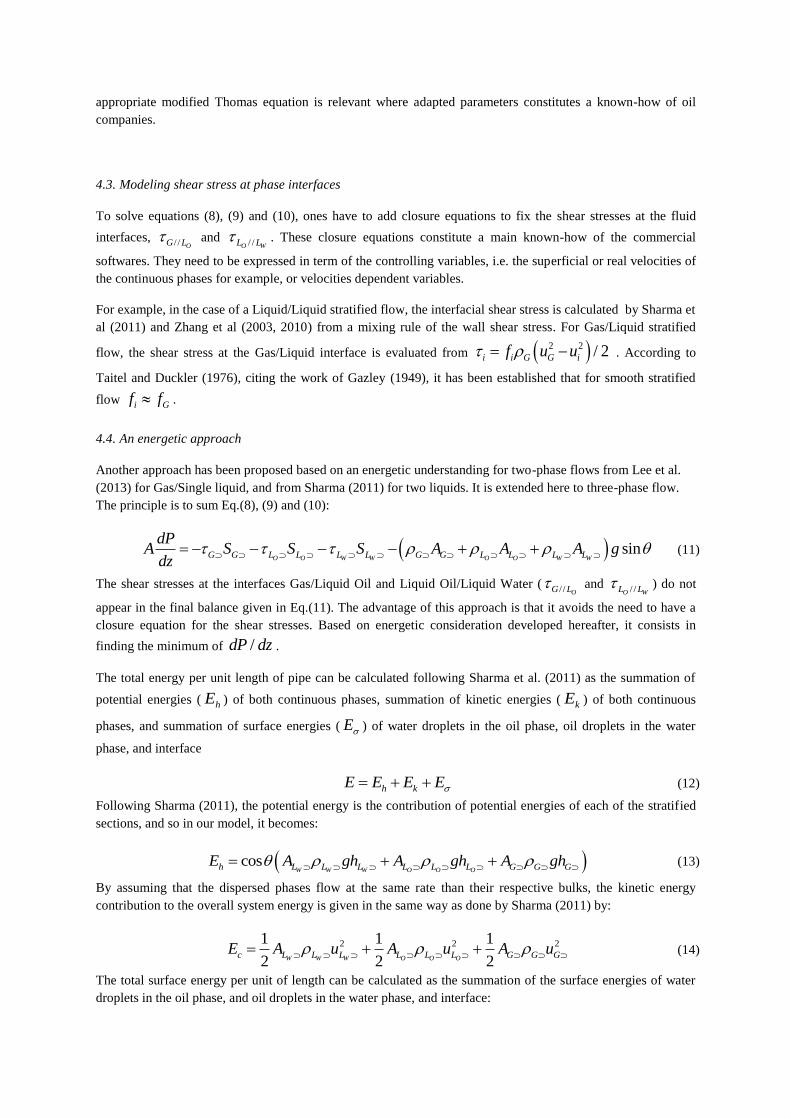
4.4. An energetic approach

Another approach has been proposed based on an energetic understanding for two-phase flows from Lee et al.

(2013) for Gas/Single liquid, and from Sharma (2011) for two liquids. It is extended here to three-phase flow.

The principle is to sum Eq.(8), (9) and (10):

sinO O W W O O W WG G L L L L G G L L L L

dPA S S S A A A g

dz (11)

The shear stresses at the interfaces Gas/Liquid Oil and Liquid Oil/Liquid Water ( / / OG L and / /O WL L ) do not

appear in the final balance given in Eq.(11). The advantage of this approach is that it avoids the need to have a

closure equation for the shear stresses. Based on energetic consideration developed hereafter, it consists in

finding the minimum of /dP dz .

The total energy per unit length of pipe can be calculated following Sharma et al. (2011) as the summation of

potential energies ( hE ) of both continuous phases, summation of kinetic energies ( kE ) of both continuous

phases, and summation of surface energies ( E ) of water droplets in the oil phase, oil droplets in the water

phase, and interface

h kE E E E (12)

Following Sharma (2011), the potential energy is the contribution of potential energies of each of the stratified

sections, and so in our model, it becomes:

cosW W W O O Oh L L L L L L G G GE A gh A gh A gh (13)

By assuming that the dispersed phases flow at the same rate than their respective bulks, the kinetic energy

contribution to the overall system energy is given in the same way as done by Sharma (2011) by:

2 2 21 1 1

2 2 2W W W O O Oc L L L L L L G G GE A u A u A u (14)

The total surface energy per unit of length can be calculated as the summation of the surface energies of water

droplets in the oil phase, and oil droplets in the water phase, and interface:

/ / / /

/ /

6 6sin sin

2 2

O W W O O W O

O W O

W O O W

L L L L L L G L

L L G L

L L L L

AH AHE D D

l l

(15)

This equation assumes an average diameter (O WL Ll ,

W OL Ll ) of the respective dispersed phases.

The solution is the condition where the total energy is a minimum (Eq.(12)), corresponding to a minimum in the

pressure drop (Eq.(11)). This type of approach has been validated for Gas/Single liquid flow modelling by Lee

et al. (2013) and for Two Liquid flow modelling by Sharma (2011). In this review, we propose to extend this

approach to three-phase flow modelling, by minimisation of the following product:

min h k

dPE E E A

dz

(16)

In the end, Eq.(16) becomes dependent on the two angular positions of the interfaces / / OG L and / /O WL L

(Figure 2), and dependent also on four fractions of the dispersed phases O WL LH ,

W OL LH , OL GH ,

WL GH .

5. Crystallization Model Implementation

As stated before, the controlling variables of a flow model description are at the number of six, and the two

angular positions of the interfaces / / OG L and / /O WL L (Figure 2), and the four fractions of the dispersed

phases O WL LH ,

W OL LH , OL GH ,

WL GH . These variables determine completely the other variables, such

as the interfacial areas and the velocities according to equation given in the appendix.

In the following part, we give the method to couple a model of crystallization to these fundamental variables.

Stating for a crystallization model, the first variables to define are the growing rate 1.G m s and a moving

surface resulting from this growing rate. As discussed in the introduction, the moving surface can be localised in

the Liquid Water ( ,wL cH ), at the interface / /O WL LS between the carrying Liquid Water ( wL ) and carrying

Liquid Oil ( OL ), or dispersed at the interface W OL La

between the Liquid Water droplets of volume fraction

W OL LH dispersed in the continuous Liquid Oil of volume fraction

,OL cH .

One has to assume a geometric model describing the specific understanding of the crystallization. We retain

here an example to support the discussion. We assume that water covers and continuously wets the hydrate

surface at the vicinity of the Liquid Oil. If Liquid Water is the continuous phase (,WL cH ), the presence of water

is unquestionable and the crystallization occurs at / / ,O WL L cS .

However, if Liquid Water is dispersed as an emulsion in the Liquid Oil, this case is more complex. Upon

hydrate formation, a crust can form isolating the Liquid Oil from the Liquid Water. If this crust is consolidated

and thick, it creates a barrier for diffusion and further hydrate growth becomes diffusion-limited by either gas

and/or water inside or outside the droplet. This type of model has very low rates of crystallization which

becomes the limiting rate and control the gas consumption rate in the end. This specific has been previously

studied by Gong (2010) and it is not the focus of the current example in which we want to emphasize the role

mass transfers in the fluid phases. Here, even if hydrates are dispersed as a crust around the water droplets, this

dispersion is wetted with water that permeates through channels from the interior of the water droplets via

microchanels (Mori and Mochizuki , 1997) or for an another source of water, such as after collision of the

hydrate particle with a unconverted water droplet.

As such, the crystallization occurs in a water medium, even if the water layer around the solid hydrate is thin. In

this water layer has a finite amount of solutes (gas). The concentration of these solutes depends on the gas

consumption rate from the growth of particle and on the gas diffusion along the different barriers, that is, the

Gas/Liquid Oil interface and interface around the particles. This section presents the hydrate growth model, the

following section will present the diffusion model from the Gas phase along the barriers discussed herein, and

the final section will present the coupling between the growth rate and gas diffusion.

If we consider the surface of the growing hydrate, the water molecules form a network of cavities that

encapsulate the gas molecules, constantly generating new site of encapsulation. The combination of water and

gas to form hydrates is non-stoichiometric and can be written as

1

5.75gS

j j s

j

n Gas Water Hydrate

(17)

1..., ,5.75gSn n are the stoichiometry factors of the formation, and

1

1gS

s j

j

n n

is a non-stoichiometry

factor relative to the probably that cavities are empty/occupied with a guest molecule.

The fundamental equation expressing the hydrate stability is deduced from statistical thermodynamics, as

originally developed by van der Waals and Platteew. It demonstrates that the hydrates become stable once the

cavities are sufficiently filled, without considering the chemical nature of the components. This point is an

important concept of our understanding, because the model yields a kinetic control of the gas composition, and a

thermodynamic control of the total gas content. The fundamental rule of clathrate hydrate stability is:

cav

H

w ( , )ln 1

β

i i

i S

T P

RT

(18)

where, R is the universal molar gas constant and i is the vector of independent occupancy factors of the

cavities. The summation is over all types of cavities (e.g., the two types of cavities, 512

and 512

62 in case of a sI

hydrate with a stoichiometry of 1 =2 and 2 6, respectively. H

w

β is the chemical potential difference of

water in the hydrate phase and water in an hypothetical empty hydrate lattice, denoted as . It can be calculated

since, at equilibrium, the chemical potential of water in the solid phase and in the liquid phase are equal, as

explained in Sloan (1998) and Sloan and Koh (2007). In case the activity of water in the liquid phase is not the

value of 1 (because of a high solubility of gases, or/and in the presence of polar molecules or even salts), the

activity coefficient L

w needs to be computed as provided for example by a simple Pitzer-Debye-Hückel model

accounting for the long range electrostatic interactions, or a more elaborate model like the eNRTL as discussed

in Kwaterki and Herri (2012). In the approach discussed here, we consider the Liquid Water to be pure water

and so L

w 1 . Complete details on the method of calculation of L

w

can be found in Herri et al. (2011).

Considering a kinetic control of the composition of the gas in the hydrate structure, and a thermodynamic

control of the total content in the cavities, the occupancy of the cavities can be correlated to the local

composition from the following equation, given in Herri and Kwaterki (2012)

g

,

11

1 (1 )i

x j i j j

j S

C x G k

(19)

where, 1.jk m s is an intrinsic kinetic constant relative to each of the components entering the structure,

,x jiC is the Langmuir constant of the solute j for the type of cavity i, 1.G m s is the growth rate, and jx is

the mole fraction of the guest at the immediate vicinity of the growing hydrate. At thermodynamic equilibrium

0G and Eq.(19) simplifies to

g

,1 1/ (1 )i x j i j

j S

C x

, which can be defined everywhere, except in the

case of unity of the Langmuir constant. In fact, the Langmuir constant is given here in terms of the mole fraction

jx of the guest component j whereas, in thermodynamic calculations at equilibrium, it is generally calculated

as ,f j iC in terms of the corresponding fugacity

jf . Expressing the relationship between the Langmuir constant

,x jiC and ,f j iC is detailed in Herri and Kwaterki (2012). The Langmuir constant is calculated following

classical methods given in Sloan (1998), Sloan and Koh (2007). It implies to determine the so-called Kihara

parameters given by Herri et al. (2011), Herri and Chassefière (2012), and Chassefière et al. (2012) for the

different types of gases of interest.

Therefore, the local thermodynamic equilibrium is obtained by satisfying the following equation:

g gcav

H

w,

,

( , )1exp 1 1 (1 )

,

iβ

W j x ji j j

j S j Si Seq Hyd

T Px C x G k

K T P RT

(20)

where, jx is the local composition outside the hydrate, and as stated earlier, it depends on the relative rate of

gas consumption from hydrate growth, and gas diffusion from the Gas phase to the immediate surroundings of

the hydrate particle crossing different barriers detailed on Figure 4, the Gas/Liquid Oil interface, rather than the

Liquid-Water-surrounding-Hydrate/Liquid Oil interface. jx is assumed to be at steady state and its value is

determined from a mass balance considering the the gas diffusion rate. This calculation is performed in the

following section.

6. Calculation of Overall Diffusion Rate Across Interfaces

Figure 4. Model of diffusion barriers from the gas phase to the water phase.

Local G/LO/LW Phase Equilibrium

Equilibrium is assumed at the interfaces only and only local equilibrium matters in our kinetic model approach.

Firstly, there is chemical equilibrium at the Gas/Liquid interface ( , / int,O Oj G L Lx ), and at the /W OL L interface (

, / / int,O W Oj L L Lx and , / / int,O W Wj L L Lx ). The local equilibrium at the Gas/Liquid interface is evaluated from the

partition coefficient.

, / int,

, /

,

O O

O

j G L L

j L G

j G

xK

x (21)

, /Oj L GK is the so-called partition coefficient, and is determined from an equation of state. Secondly, there is

chemical equilibrium at the interface between the solutes in the bulk OL and WL phases,

, / / int,

, , /

, / / int,

O W O

O W

O W W

j L L L

x j L L

j L L L

xX

x (22)

, , /O Wx j L LX is a partition coefficient of solutes j expressed in term of molar fraction x between the OL and WL

phases, and it can be calculated from the Henry’s constant in water:

, / / int, , , ,

, , /

, , /, / / int, H, , , ,exp

O W O

O W

OO W W W O

j L L L j G j G j G

x j L L

x j G Lj L L L x j L j L

x x x PX

Xx k Pv RT

(23)

H, , , ,

, , /

, , , /

exp 1W O

O W

O

x j L j L

x j L L

j G x j G L

k Pv RTX

P X

(24)

where H, , , Wx j Lkis the Henry’s constant of component j in liquid water and ,j G is the coefficient of fugacity j

in the gas phase at pressure P.

Mass Transfer at the G//L O Interface

The gas transfer rate at the Gas// OL interface is given as the product of the interfacial area 2

// /OG LS m m

and the surface mass transfer rate. The surface mass transfer rate1 2. .mole s m is given by:

1 2

/ , , , , / / int, , , , / / in, ,. .O O

G LG L j x G j G j G L G j x L j G L L j L

G L

J mole s m k x x k x xM M

(25)

(a)

(b)

Figure 5 : Mass transfer across a gas/liquid interface: (a) both liquid side and gas side are limiting rate, and (b) only liquid side is limiting rate.

Micro-models are required to model this interphase transport of mass that often takes place in combination with

a chemical reaction. Frequently applied micro-models are the stagnant film model in which mass transfer is

postulated to proceed via stationary molecular diffusion in a stagnant film of thickness l (Lewis and Whitman

,1924, /k l D ), the penetration model in which the residence time of a fluid element at the interface is the

characteristic parameter (Higbie,1935), and the surface renewal model in which a probability of replacement is

introduced (Danckwerts, 1951).

All of these micro-models assume the presence of a well-mixed bulk liquid. Mass transfer under the specific

case of laminar flow has been studied over the last decades by Boyadjiev and co-workers. Their original study

dated from 1978, proposed an original treatment of the equation of mass transfer that has been simplified over

the years. Their main concern is that in the conditions of fast mass transfer, the kinetics of mass transfer exhibits

effects which cannot be described by the linear theory of diffusion in the boundary layer approximation. They

therefore developed a non-linear theory of mass transfer and applied it in the study of “gas-liquid” systems.

They also conducted many experimental studies to support the model. All that work is summarized in Boyadjiev

and Babak (2000). We present here only the specific cases where diffusion is limited on the gas side or on the

liquid side. For the case with diffusion limited in the liquid side,

L L 2

2Sh Pe

Eq.(26); Sherwood number Sh

kl

D Eq.(27); Peclet number Pe

ul

D Eq.(28)

where the functions 1 and 2 are,

1L

G

u

u Eq.(29); and

1/2 1/2

3/2 3/2

2,2000 1 2,1978 1G G G G

L L L L

(30)

There are two forms proposed for 2 in Boyadjiev and Babak (2000) and Mitev and Boyadjiev (1978), but for

one purposes, we use 2,2000 as the applicable one.

1/2 1/2

3/2

2,2000 1G G

L L

(31)

The other variable given in Boyadjiev and Babak (2000) is 0.33205 .

Mass Transfer at the LO //LW Interface

We can assume a dispersion of a phase (the water) in another phase (the liquid oil). Moreover, we have to

assume an average diameter of the dispersed water in oil to be given by W OL Ll , with the water droplet

considered as a particle. The rate of gas consumption (per unit length of pipe) of component j around a particle

is given by:

1

, , , , bulk , int. Lj j x j j

L

r mole m d a A x xM

, (32)

where 2A m

is the cross sectional interfacial area of the carrying phase (see figure Figure 2) and

2 3.a m m

is the surface area of droplets of phase dispersed in carrying phase , , bulkjx is the

mole fraction of j in the bulk phase, and , ,j x Ld (1ms ) the mass transfer coefficient of the guest species j

around the particle, respectively. , ,j xd can be estimated from a classical correlation between the

dimensionless Reynolds, Sherwood and Schmidt numbers of/around the crystal particle (index “P”), ReP , ShP

and Sc , for example, as done by Armenante and Kirwan (1989),

0.52 1 3Sh 2 0.52Re ScP P (33)

, ,

PShj x

j

d l

D

,

4/3 1/3

ReP

l

, Sc

jD

(34)

In the equations above, l is the particle diameter and / is the kinematic viscosity of the liquid phase,

approximated by the kinematic viscosity of the pure solvent. jD (2 1[ ] m sjD ) denotes the diffusivity of the

gas in the solvent.

The dissipation energy per unit mass can be estimated from Angelli and Hewitt (2000)

3

2

uf

d

(35)

7. Overall Gas Diffusion Rate

The modelling of the overall diffusion rate is the connecting equation between the thermodynamic, the flow

mechanics and the kinetics because it fixes the relationships between the compositions.

Once the interface gas transfer properties are fixed, it is possible to write successive mass balance at steady state

across the different interfaces. On one hand, gas is fed at the gas/liquid interface, Eq.(25), and on the other hand,

it is transferred to the growing hydrate via the water diffusion layer around the particles, Eq. (32). The specific

example presented here considers a dispersion of water droplets in the oil. During crystallisation, the droplets

are covered with hydrates but a thin liquid water layer remains around the particles. It is finally possible to

express all the intermediate gas molar fraction as a function of the two limit conditions, first being the gas molar

fractions ,j Gx , and second being the molar fractions of species at the immediate vicinity of the growing hydrate

, / / int,W Wj H L Lx , for example:

,

, , / , / / int,

, , /

, ,1

O W O W W

O

O

j G

x j L L j L L L j

x j G L

j bulk L

j

xX x B

Xx

B

(36)

O W

, , / ,

, L //L int, , / / int,

, , /

11 1

O W

W W W

O

x j L L j j j G

j L j H L L

j j j j x j G L

X B B xx x

A B B A X

(37)

With

with

0

,

,

W W O

O W

j L L L

j

j L L L

d MA

d M

(38)

0

, , / /

, / /

O O

W O

j x L G L

j

j L L L

k SB

d S (39)

Constants jA and jB contains the geometrical properties of the interfaces / / OG LS and

/ / WH LS (given from the

flow model), the partition coefficients (given from the local thermodynamic model), and physical properties,

such as the diffusion coefficients, densities and molar mass.

As a result, this mass transport-based equation is coupled to the local thermodynamic equilibrium at the hydrate

surface, which is given in the next subsection.

8. Dynamic Hydrate Equilibrium

We propose here a local description of the growth which is independent of the different approaches of the

litterature. We can consider only the Solid/Liquid interface with its interface layers, and write a mass balance.

In fact, the composition of the gas hydrate can be evaluated from the mass balance in the liquid layer around the

particle. At steady state, there is equality between the integration rate due to the Langmuir type of enclathration

(left-hand-side) and the gas diffusion (right-hand-side):

O W

gcav

/ / , / / , L //L int, , / / int,W

W W W O W W W

W

L

H L i ji j L L L j L j H L Lj S

i S L

GS c d S x xM

, (40)

where O W, L //L int, Wj Lx is the mole fraction of j at the interface between the water liquid surrounding the hydrate

particle and the oil, , / / int,W Wj H L Lx is the mole fraction of j at the interface between the water liquid

surrounding the hydrate particle and the hydrate surface. , Wj Ld (1

,[ ] msWj Ld ) is the mass transfer

coefficient of the guest species j around the crystal, respectively. wL and

wLM stands for the density (

w

3[ ] kg mL ) and the molar mass (

w

1[ ] g molLM ) of the solvent (water), respectively. 3.ic mole m

is the concentration of cavity type i in the structure of the hydrate. j i is the occupancy factor of this cavity

type i by a component type j. As given by Herri and Kwaterski (2012), under non-equilibrium condition, the

occupancy assumes a similar form to Eq.(19):

g

, , int

, , int '

(1 )

1 (1 )

x j i j j

j i

x j i j j

j S

C x G k

C x G k

, (41)

Once numerical values for jk (1[ ] msjk ) and for G are determined, the , / / int,W Wj H L Lx values can be

calculated as the solution for the system of N non-linear equations. This set of equations is obtained by

substituting the expressions for j i into Eq.(40)

O W

gcav

g

, , / / int,

, , L //L int, , / / int,

, , / / int, '

(1 )

1 (1 )

W W W

W W W W

W W W

x ji j H L L j L

i j L j L j H L Lj S

i S x j i j H L L j L

j S

C x G kG c d x x

C x G k M

(42)

where the quantity , W W Wj L L Ld M has the dimension of a molar flux and thus

2 1

,[ ] mol m sW W Wj L L Ld M . This last equation completely accounts as the relationship expressing the

hydrate stability in Eq. (20).

Finally, the local equilibrium is defined when the values of and , / / int,W Wj H L Lx for all gj S satisfying

both Eq.(42) and Eq. (20). The calculation procedure is outlined in detail in Figure 6. At each step of

G

calculation, all the composition variables in the Gas/Liquid system are fixed from , / / int,W Wj H L Lx and

,j Gx :

,int / , , / ,O Oj G L L j G L j Gx K x is calculated from local thermodynamic equilibrium at the / OG L interface from the

partition coefficient , / Oj G LK . O W, L //L int, Wj Lx is calculated from Eq.(37),

O W, L //L int, Oj Lx from Eq.(22), and

, , Oj bulk Lx from Eq.(36). The composition in the gas ,j Gx is fixed. The final value of , / / int,W Wj H L Lx needs to

satisfy both Eq. (42) and Eq. (20).

The initial values of , / / int,0W Wj H L Lx is determined assuming the corresponding solubilities are at

thermodynamic equilibrium at pressure ,,eq j GP T x , temperature T, and composition of gas ,j Gx .

The procedure for the calculation is with a double convergence loop. At a given growth rate G, in the first

loop, iterations are performed on , / / int,W Wj H L Lx in order to satisfy Eq.(42). Once converged, the mass transfer

rates in each of the interface layers are identical. Then a second convergence loop is performed on the growth

rate to satisfy the hydrate local thermodynamic equilibrium given in Eq.(20).

From a physical point of view, G is the value at which the structure can grow by incorporation of solute gas

to such an amount that is sufficient for stabilising the hydrate structure (i.e., the minimum occupancy of the

cavities). The relative proportion to which the different gas molecules j enter the hydrate structure is

determined in the first convergence loop, which is an indirect consequence of the competition between the

diffusion rates around the crystals and integration rates in the structure. By this competition the , intjx values are

fixed.

Figure 6. Procedure of calculation of the thermo-kinetic equilibrium.

9. Conclusion

We present in the conclusion a running test of the model implemented in an excell sheet. We evaluate the

maximum growing rate, and in the end the final time of total water consumption of a stratified flow, consisting

of a gas phase phase (6.1%CO2, 88.4%CH4, 1.2%ethane, 1.2%propane, 1.2%ethane, 1.2%n-butane,

1.2%butane) and an emulsion of water in an oil (decane).

The flow pressure is 40 bars, and the temperature is 1°C. The hydrate equilibrium pressure is 15.4 bars. The

input parameters are given in the Table 1 after running the thermodynamic package given in section 3.

The geometry of the flow is given in Table 2 after outputting the flow calculation package given in section 4

based on the minimization of energy. It gives the position of G/LO interface, and as a consequence the real

velocities. The water is considered as fully dispersed in the oil.

Then, gas transfer rates and crystal growth rate G can be calculated based on procedures given is sections 5 to 8

and resumed in Figure 6. The growth rate is water droplets size dependent, as showed in Figure 7. We can see

that the growth rate can never be higher than 1.8 mm/s. The maximum growing rate corresponds to a balance

between the mass diffusion limiting steps at the gas/liquid interface and at the solid/liquid interface. Figure 8

shows the corresponding time of full conversion of the water molecules into hydrates. The higher the droplet

size, the higher the time of conversion. As an example, for an emulsion of initial size 1000-2500 mm, the time

of total water conversion is lower than 5-10 min.

Figure 7. Hydrate growth rate depending on the size of the dropplets.

Figure 8. Final time of total water molecules consumption to from a fully dispersion of solid in the oil flow

Table 1. Input parameters after outputting the thermodynamic package given in section 3

Superficial velocities

Densities Viscosities Surface tensions

Pipe diameter Absolute pipe roughness

Pipe inclination

[m/s] [kg/m3] [Pa.s] [N/m] [m] [m] [rad]

v 0.27 0 0

G 4,7 100 1.60E-5

LO 0,3 735 5.20E-4

LW 0,01 1028 1.92E-3

/O WL L 0.036

/ OG L

0.0061

Table 2. Output geometric parameters after outputting the flow modelling package given in section 4

real velocities

Position of interfaces

[m/s] [rad]

u 0/G L

0 / WL L

G 3.98 1.79 0

LO 0.16

LW 0.16

References

Abduvayt, P., Manabe, R., Watanabe, T., Arihara, N., 2006. Analysis of oil/water-flow tests in horizontal, hilly terrain and vertical pipes.

SPE Prod. Oper., 123–133.

Angeli, P, Hewitt, GF, 2000a, Drop size distributions in horizontal oil-water dispersed flows. Chemical Engineering Science 55 (2000) 3133–43.

Angeli, P., Hewitt, G.F., 2000b, Flow structure in horizontal oil–water flow. Int. J. Multiphase Flow 26 (2000) 1183–1203.

Armenante, P.M., Kirwan, D.J., Mass transfer to micro particles in agitated vessels, Chem. Eng. Sci., 44 (1989) 2781-2796 Boyadjiev, C. B., 1972, Theor. Osn. Khi. Techn. 6 (1972) 118

Boyadjiev, C. B., Babak, V. N., 2000, Non-Linear Mass Transfer and Hydrodynamic Stability, 2000,1 -16

Chassefière, E., Dartois, E., Herri, J.M., Tian, F., Mousis, O., Lakhlifi, A., Schmidt, F., 2012, CO2-SO2 clathrate hydrate formation on early

Mars, Icarus 223 (2012) 878-891

Danckwerts, P.V., 1951. Significance of liquid-film coefficients in gas absorption. Industrial and Engineering Chemistry 43 (1951) 1460–

1467.

Danesh, A., 1998, PVT Phase behaviour of petroleum reservoir fluids, elsevier Einstein, A. , Investigations on the theory of Brownian motion, Ann Phys Leipzig 19 (1906) 289.

Fidel Dufour, A., Gruy, F., Herri, J.M., 2006, Rheology of methane hydrate slurries during their crystallization in a water in dodecane

emulsion under flowing, Chemical Engineering Science 61 (2006) 505–515 Gazley, C., 1949, Intertacial Shear and Stability in Two-Phase Flow,” PhD theses, Univ. Del., Newark

Gong J., Shi B., Zhao J., Natural gas hydrate shell model in gas-slurry pipeline flow, Journal of Natural Gas Chemistry, 2010, 19, 261–266

Graham, A.L. , Steele, R.D. , Bird, R.B. , Particle clusters in concentrated suspensions. 3. Prediction of suspension viscosity, Ind Eng Chem Fundam 23 (1984) 420–425.

Handa, Y. P., 1986, Composition Dependance of Thermodynamic Properties of Xenon Hydrate, J. Phys. Chem. 90 (1986) 5497-5498

Hayduk, W., and B. S. Minhas, 1982, Can. J. Chem. Eng., 60 (1982) 295 Herri J.-M., Bouchemoua A., Kwaterski , M., Fezoua A., Ouabbas Y., Cameirao A., 2011, Gas Hydrate Equilibria from CO2-N2 and CO2-

CH4 gas mixtures, – Experimental studies and Thermodynamic Modelling, Fluid Phase Equilibria, Vol. 301, pages 171-190

Herri, J.M., Chassefiere E., 2012, Carbon dioxide, argon, nitrogen and methane clathrate hydrates: thermodynamic modelling, investigation of their stability in Martian atmospheric conditions and variability of methane trapping, Planetary and Space Science 73 (2012), pp.

376-386

Herri, J.M., Kwaterski, M., 2012, Derivation of a Langmuir type of model to describe the intrinsic growth rate of gas hydrates during crystallization from gas mixtures, Chemical Engineering Science 81 (2012) 28-37

Hester, K.C., Huo, Z., Ballard, A.L., Koh, C.A., Miller, K.T., Sloan, E.D., 2007, Thermal Expansivity for sI and sII Clthrate Hydrates, J.

Phys. Chem. B, 111, 8830-8835

Higbie, R., 1935. The rate of absorption of a pure gas into a still liquid during a short time of exposure. Transactions of the American

Institute of Chemical Engineers 31 (1935) 365–389.

Holder, G. D. , Corbin, G., Papadopoulos, K. D., 1980, Thermodynamic and molecular proprieties of gas hydrates from mixtures containing Methane Argon and Krypton. Ind Eng Chem Fund. 19 (1980) 282.

Kwaterski, M., and Herri, J.M., 2012, Modelling Gas Hydrate Equilibria using the Electrolyte Non-Random Two-Liquid (eNTRL) Model, Fluid Phase Equilibria, Volume 371, 15 June 2014, Pages 22-40

Lee, H., Al-Sarkhi, A., Pereyra, E., Sarica, C., Park, C., Kang, J., Choi, J., Hydrodynamics model for gas–liquid stratified flow in horizontal

pipes using minimum dissipated energy concept, Journal of Petroleum Science and Engineering 108 (2013) 336–341 Lee, B.I., Kesler, M.G., 1975, A Generalised Thermodynamics Correlation Based on Three-Parameters Corresponding States, AIChE J. 21-

4 (1975) 510-527

Lewis, W.K., Whitman, W.G., 1924, Ind.Eng. Chem. 16 (1924) 1215 Mckoy, V. , Sinagoglu, O.J., 1963, Theory of dissociation pressures of some gas hydrates, J. Chem. Phys. 38 (1963) 2946.

Mills, P., 1985. Non Newtonian behaviour of flocculated suspensions. Journal de Physique—Lettres 46, L301–L309

Mitev, P., Boyadjiev, C., 1978, Mass Transfer in Cocurrent Gas-Liquid Stratified flow, Letters in Heat and Mass Transfer 5-6 (1978) 349-354

Mori Y.H., Mochizuki T., Mass transport across clathrate hydrate films-a capillary permeation model, Chem. Eng. Sci., 1997, 52, 3613–

3616 Palermo T., Fidel-Dufour A., Maurel P., Peytavy J.L., Hurtevent, C. (2005) Model of hydrates agglomeration - Application to hydrates

formation in an acidic crude oil, BHR Group 2005 Multiphase Technology, Barcelone.

Parrish, W.R. , Prausnitz, J.M. 1972, Dissociation pressure of gas hydrates formed by gas mixtures, Ind. Eng. Chem. Process Dev. 11

(1972) 26–35.

Peng, D.Y. and Robinson D.B., Industrial and Engineering Chemistry Fundamentals, 15 (1976) 59

Poling, B.E., Prausnitz, J.M., O’Connel, J.P., 2001, The properties of gases and liquids, McGraw-Hill, ISBN 0-07-011682-2 Sloan, E.D.; 1998, Clathrate hydrates of natural gases; 2nd ed., Marcel Decker, New York.

Sloan., E.D.; Koh, C.A.; 2008, Clathrate hydrates of natural gases”; 3rd ed., CRC Press, Boca Raton

Sharma, A., Al-Sarkhi, A., Sarica, C., Zhang, H.Q., Modelling of oil–water flow using energy minimization concept, Int. J. Multiphase Flow 37 (2011) 326–335

Taitel, Y., and Dukler, A. E, 1976, A theoretical approach to the Lockhart-Martinelli correlation for stratified flow, Int. J. Multiphase Flow 2

(1976) 591–595

Taitel, Y., Dukler, A.E., 1976b, A model for predicting flow regime transitions in horizontal and near horizontal gas‐liquid flow, AIChE Journal 22-1 (1976) 47-55.

Thomas, D.G., 1965. Transport characteristics of suspensions: VII. A note on the viscosity of Newtonian suspensions of uniform spherical

particles. Journal of Colloid Science 20, 267–277 Uchadin, K.A.; Ratcliffe. C.I.; Ripmeester, J.A.; 2002, Single Crystal Diffraction Studies of Structures I. II and H Hydrates: Structure, Cage

Occupancy and Composition; J. Supramol. Chem. 2 (2002) 405-408.

van der Waals, J. H.; Platteeuw, J. C.; “Clathrate solutions”; Adv. Chem. Phys. 2, (1959) l-57. Von Stackelberg, M.; Müller, H. R.; 1951, On the structure of gas hydrates; J. Chem. Phys. 19 (1951) 1319-1320.

Wilke, C.R.; Chang, P., Correlation of Diffusion Coefficients in Dilute Solution, AIChE J., 1 (1955) 264-270

Zhang, H.Q., Wang, Q., Sarica, C., Brill, J.P., Unified model for gas–liquid pipe flow via slug dynamics—part I: model development, ASME J. Energy Res. Technol. 125-12 (2003a) 266–273.

Zhang, H.Q., Wang, Q., Sarica, C., Brill, J.P., Unified model for gas–liquid pipe flow via slug dynamics— part II :model validation., ASME

J. Energy Res. Technol. 125-12 (2003b) 274–283. Zhang, H.-Q., Sarica, C., 2006., Unified modeling of gas/oil/water pipe flow – basic approaches and preliminary validation. SPE Projects

Facil. Constr. 1, 1–7..