Embed Size (px)
Citation preview
Modeling of asphaltene precipitation from n-alkanediluted heavy oils and bitumens using the PC-SAFTequation of stateZúñiga-hinojosa, María A.; Justo-garcía, Daimler N.; Aquino-olivos, Marco A.; RomanRamirez, Luis; García-sánchez, FernandoDOI:10.1016/j.fluid.2014.06.004
License:Other (please specify with Rights Statement)
Document VersionPeer reviewed version
Citation for published version (Harvard):Zúñiga-hinojosa, MA, Justo-garcía, DN, Aquino-olivos, MA, Román-ramírez, LA & García-sánchez, F 2014,'Modeling of asphaltene precipitation from n-alkane diluted heavy oils and bitumens using the PC-SAFTequation of state' Fluid Phase Equilibria, vol 376, pp. 210-224. DOI: 10.1016/j.fluid.2014.06.004
Link to publication on Research at Birmingham portal
Publisher Rights Statement:NOTICE: this is the author’s version of a work that was accepted for publication in Fluid Phase Equilibria. Changes resulting from thepublishing process, such as peer review, editing, corrections, structural formatting, and other quality control mechanisms may not bereflected in this document. Changes may have been made to this work since it was submitted for publication. A definitive version wassubsequently published in Fluid Phase Equilibria, Vol 376, August 2014, DOI: 10.1016/j.fluid.2014.06.004.
Eligibility for repository checked April 2015
General rightsUnless a licence is specified above, all rights (including copyright and moral rights) in this document are retained by the authors and/or thecopyright holders. The express permission of the copyright holder must be obtained for any use of this material other than for purposespermitted by law.
•Users may freely distribute the URL that is used to identify this publication.•Users may download and/or print one copy of the publication from the University of Birmingham research portal for the purpose of privatestudy or non-commercial research.•User may use extracts from the document in line with the concept of ‘fair dealing’ under the Copyright, Designs and Patents Act 1988 (?)•Users may not further distribute the material nor use it for the purposes of commercial gain.
Where a licence is displayed above, please note the terms and conditions of the licence govern your use of this document.
When citing, please reference the published version.
Take down policyWhile the University of Birmingham exercises care and attention in making items available there are rare occasions when an item has beenuploaded in error or has been deemed to be commercially or otherwise sensitive.
If you believe that this is the case for this document, please contact [email protected] providing details and we will remove access tothe work immediately and investigate.
Download date: 10. May. 2018

Accepted Manuscript
Title: Modeling of asphaltene precipitation from n-alkanediluted heavy oils and bitumens using the PC-SAFT equationof state
Author: Marıa A. Zuniga-Hinojosa Daimler N. Justo-GarcıaMarco A. Aquino-Olivos Luis A. Roman-Ramırez FernandoGarcıa-Sanchez
PII: S0378-3812(14)00337-9DOI: http://dx.doi.org/doi:10.1016/j.fluid.2014.06.004Reference: FLUID 10147
To appear in: Fluid Phase Equilibria
Received date: 7-4-2014Revised date: 30-5-2014Accepted date: 2-6-2014
Please cite this article as: M.A. Zuniga-Hinojosa, D.N. Justo-Garcia, M.A. Aquino-Olivos, L.A. Roman-Ramirez, F. Garcia-Sanchez, Modeling of asphaltene precipitationfrom n-alkane diluted heavy oils and bitumens using the PC-SAFT equation of state,Fluid Phase Equilibria (2014), http://dx.doi.org/10.1016/j.fluid.2014.06.004
This is a PDF file of an unedited manuscript that has been accepted for publication.As a service to our customers we are providing this early version of the manuscript.The manuscript will undergo copyediting, typesetting, and review of the resulting proofbefore it is published in its final form. Please note that during the production processerrors may be discovered which could affect the content, and all legal disclaimers thatapply to the journal pertain.

Page 1 of 42
Accep
ted
Man
uscr
ipt
28
Modeling of asphaltene precipitation from n-alkane diluted heavy oils and bitumens using the PC-SAFT equation of state
María A. Zúñiga-Hinojosa1, Daimler N. Justo-García2, Marco A. Aquino-Olivos3,
Luis A. Román-Ramírez4, and Fernando García-Sánchez1,*
1 Laboratorio de Termodinámica, Programa de Investigación en Ingeniería Molecular, Instituto Mexicano del Petróleo. Eje Central Lázaro Cárdenas 152, 07730 México, D.F., México.
2 Departamento de Ingeniería Química Petrolera, ESIQIE, Instituto Politécnico Nacional, Unidad Profesional Adolfo López Mateos, 07738 México, D.F., México.
3 Programa de Aseguramiento de la Producción de Hidrocarburos, Instituto Mexicano del Petróleo. Eje Central Lázaro Cárdenas 152, 07730 México, D.F., México.
4 School of Chemical Engineering, University of Birmingham, Edgbaston, Birmingham B15 2TT, United Kingdom.
_____________________________________________________________________________________
ABSTRACT In this work, the PC-SAFT equation of state was applied to the modeling of asphaltene precipitation from n-alkane diluted heavy oils and bitumens. Liquid-liquid equilibrium was assumed between a dense liquid phase (asphaltene-rich phase) and a light liquid phase. The liquid-liquid equilibrium calculation, in which only asphaltenes were allowed to partition to the dense phase, was performed using an efficient method with Michelsen’s stability test. The bisection or Newton-Raphson method was used to improve convergence. Experimental information of the heavy oils and bitumens, characterized in terms of solubility fractions (saturates, aromatics, resins, and asphaltenes), was taken from the literature. Asphaltenes were divided into fractions of different molar masses using a gamma distribution function. Predictions of the PC-SAFT equation of state using linear correlations of the binary interaction parameters between asphaltene subfractions and the n-alkane were compared with the measured onset of precipitation and the amount of precipitated asphaltene (fractional yield) of the heavy oils and bitumens diluted with n-alkanes. Results of the comparison showed a satisfactory agreement between the experimental data and the calculated values with the PC-SAFT equation. Key words: onset; asphaltene precipitation; equation of state; PC-SAFT; liquid-liquid equilibrium. _____________________________________________________________________________________
* Corresponding author. Tel.: +52 55 9175 6574. E-mail: [email protected]

Page 2 of 42
Accep
ted
Man
uscr
ipt
29
1. Introduction
Asphaltenes are defined as the fraction of crude oil or bitumen that precipitates with the addition of a low-
chain liquid n-alkane (n-pentane or n-heptane) and dissolves in aromatic solvents as toluene or benzene.
In practice, there are different aspects of the asphaltene precipitation that are important for the oil industry
such as the prevention of the plugging in transport pipelines and the damages caused in the refinery
facilities due to the asphaltene precipitation process. A major problem is when different crude oils having
different densities and viscosities are mixed and they are, in turn, mixed with light liquid hydrocarbons
(e.g., natural gasolines) to reduce the viscosity of the crude oil blends, since asphaltene precipitation may
occur due to the instability of the crude oil mixtures [1].
To overcome such a problem, various research groups have developed different approaches to predict and
quantify the onset and amount of precipitated asphaltene in crude oils. This task was started with the
approach of Hirschberg et al. [2], who applied the regular solution theory for modeling asphaltene
precipitation in crude oils. Later, this modeling approach was improved by other authors to predict (1) the
amount of precipitated asphaltene from n-alkane diluted heavy oils and bitumens [3, 4], (2) the
asphaltenes dissolved in pure solvents [5, 6], and (3) the stability of crude oil blends [1, 7]. In particular,
Yarranton and co-workers [1, 3, 4] proposed approaches to predict asphaltene precipitation by treating
them as a mixture of subfractions with different densities and molar masses. These approaches have been
successfully applied to several heavy oils and bitumens diluted with n-alkanes [3, 4]. The heavy oils and
bitumens were characterized based on SARA analysis and the polidispersity of the asphaltene fraction
was included through the use of a gamma distribution function.
Other approaches in which the asphaltene precipitation is understood as a result of self-assembly and
instability of resinous-asphaltene aggregates in the crude oil have also been used. For instance, Leontaritis
and Mansoori [8] presented a colloidal model based on the assumption that the insoluble solid asphaltene
particles are suspended in the crude oil; the suspended solid asphaltene particles being stabilized by the
adsorbing resins on their surface. In this model, resins are necessary for the asphaltenes to exist in
solution. Subsequently, Victorov and Firoozabadi [9], Pan and Firoozabadi [10], and Victorov and
Smirnova [11], among others, presented thermodynamic models to predict asphaltene precipitation in
petroleum fluids by assuming that asphaltene precipitation from petroleum fluid is a micellization
process. These models, however, although have shown promising results in explaining most of the
experimentally observed results, they are still far from provides satisfactory quantitative representation.

Page 3 of 42
Accep
ted
Man
uscr
ipt
30
On the other hand, the application of an equation of state to calculate the asphaltene solubility in solvents
was studied by Gupta [12] considering a solid-liquid equilibrium calculation. Nghiem and co-workers
[13-15] applied a modeling technique based on the representation of the precipitated asphaltene as a pure
dense phase. In this approach, the heaviest component in the oil is divided into two fractions, the non-
precipitating and the precipitating fraction. The precipitating fraction is considered as pure asphaltenes
and the prediction precipitation process is quantified by a three phase flash calculation. Sabbagh et al.
[16] applied in their approach a liquid-liquid equilibrium calculation, where one of the liquid phases is
considered a light phase or a non-precipitating phase and the other liquid phase is considered a heavy
liquid phase or a precipitating phase. The precipitating phase is considered a phase where only
asphaltenes are present. They used the PR equation of state [17] to represent the asphaltene-rich liquid
phase by relating the equation of state parameters of each asphaltene fraction to monomer parameters
using group contribution theory. Ting et al. [18] modeled the asphaltene phase behavior in a model live
oil and a recombined oil under reservoir conditions by using the SAFT equation of state [19]. In this case,
the parameters of the equation of state for the asphaltenes were adjusted to precipitation data from oil
titrations with n-alkanes at ambient conditions.
By using a molecular-thermodynamic framework based on the SAFT equation of state and colloidal
theory, Wu et al. [20, 21] calculated the solubility of asphaltenes in petroleum liquids as a function of
temperature, pressure, and liquid-composition. In this approach, asphaltenes and resins were represented
by pseudo-pure components while all other components in the solution were represented by a continuous
medium that affects interactions among asphaltene and resin particles. The effect of the medium on
asphaltene-asphaltene, resin-asphaltene, and resin-resin pair interactions was taken into account through
its density and dispersion-force properties. The SAFT model was used in the framework of McMillan-
Mayer theory, which considers hard-sphere repulsive, association and dispersion-force interactions. In
their calculations, Wu et al. assumed that asphaltene precipitation is a liquid-liquid equilibrium process.
Buenrostro-Gonzalez et al. [22] used an approach similar to that suggested by Wu et al. for modeling the
asphaltene precipitation from n-alkane diluted Mexican crude oils. They used the statistical association
fluid theory for potentials of variable range (SAFT-VR) equation of state [23] in the framework of the
McMillan-Mayer theory in the calculations to represent the asphaltene precipitation envelopes and bubble
point pressures of the two oils investigated. By matching a single titration curve or two precipitation onset

Page 4 of 42
Accep
ted
Man
uscr
ipt
31
points with this SAFT-VR equation of state, satisfactory predictions of asphaltene precipitation over wide
temperature, pressure, and composition intervals were obtained.
Li and Firoozabadi applied the cubic-plus-association (CPA) equation of state [24] to study the asphaltene
precipitation from solutions of toluene and an n-alkane and from n-alkane diluted heavy oils and
bitumens [25], and the asphaltene precipitation in live oils from temperature, pressure, and composition
effects [26]. Heavy oils and bitumens were characterized in terms of saturates, aromatics/resins, and
asphaltenes, whereas the live oils were characterized by considering the pure components, the pseudo-
hydrocarbon components, and the hydrocarbon residue. In the case of heavy oils and bitumens, the
asphaltene precipitation was modeled as liquid-liquid equilibrium. By using a single adjustable parameter
−the cross association energy between asphaltene and aromatics/resins (or toluene), the amount of
asphaltene was successfully predicted over a broad range of temperatures, pressures, and compositions
for n-alkane diluted model solutions, heavy oils, and bitumens. In the case of live oils, the asphaltene
precipitation was modeled as liquid-liquid equilibrium between the upper onset and bubble point
pressures and as gas-liquid-liquid equilibrium between the bubble point and lower onset pressures. The
amount and onset pressures of asphaltene precipitation in several live oils were reasonably reproduced
over a broad range of composition, temperature, and pressure conditions.
More recently, Panuganti et al. [27] presented a procedure to characterize crude oils and plot asphaltene
envelopes using the PC-SAFT equation of state. The results obtained with the proposed characterization
method showed a satisfactory matching with the experimental data points for the bubble point and
asphaltene precipitation onset curves studied.
The aim of this work is to apply the PC-SAFT equation of state [28] to predict the asphaltene
precipitation from n-alkane diluted heavy oils and bitumens by using linear correlations of the binary
interaction parameter as a function of n-alkane concentration. It is assumed that there exists liquid-liquid
equilibrium coexistence between a light non-precipitating liquid phase and a heavy precipitating liquid
phase, where only asphaltenes are allowed to partition, and that the effect of self-association is included
in the asphaltene molar mass distribution to model the asphaltene precipitation from solvent diluted heavy
oils and bitumens. The oils are characterized in terms of saturates, aromatics, resins, and asphaltenes
(SARA) fractions, and the asphaltenes are, in turn, treated as nano-aggregates formed from asphaltene
monomers and divided into subfractions of different aggregation number based on a gamma distribution
function.
Page 5 of 42
Accep
ted
Man
uscr
ipt
32
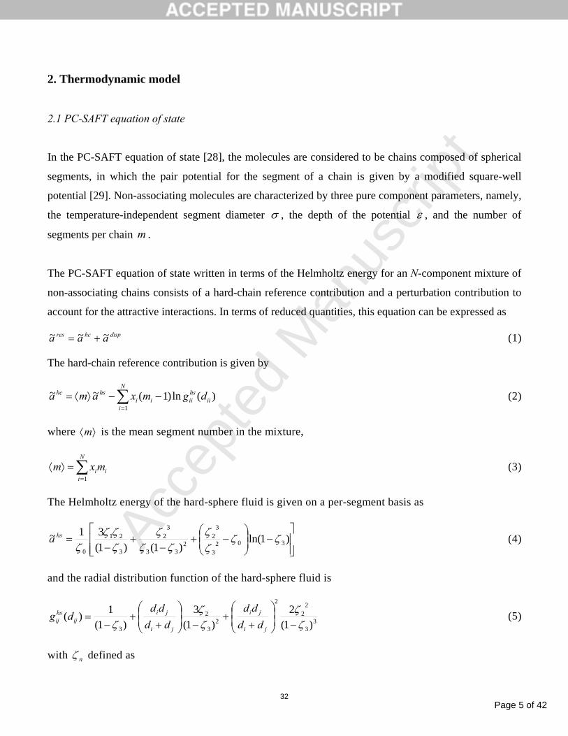
2. Thermodynamic model
2.1 PC-SAFT equation of state
In the PC-SAFT equation of state [28], the molecules are considered to be chains composed of spherical
segments, in which the pair potential for the segment of a chain is given by a modified square-well
potential [29]. Non-associating molecules are characterized by three pure component parameters, namely,
the temperature-independent segment diameter σ , the depth of the potential ε , and the number of
segments per chain m .
The PC-SAFT equation of state written in terms of the Helmholtz energy for an N-component mixture of
non-associating chains consists of a hard-chain reference contribution and a perturbation contribution to
account for the attractive interactions. In terms of reduced quantities, this equation can be expressed as
disphcres aaa ~~~ += (1)
The hard-chain reference contribution is given by
∑=
−−⟩⟨=N
iii
hsiiii
hshc dgmxama1
)(ln)1(~~ (2)
where ⟩⟨m is the mean segment number in the mixture,
∑=
=⟩⟨N
iiimxm
1 (3)
The Helmholtz energy of the hard-sphere fluid is given on a per-segment basis as
⎥⎥⎦
⎤
⎢⎢⎣
⎡−⎟⎟
⎠
⎞⎜⎜⎝
⎛−+
−+
−= )1ln(
)1()1(31~
3023
32
233
32
3
21
0
ζζζζ
ζζζ
ζζζ
ζhsa (4)
and the radial distribution function of the hard-sphere fluid is
33
22
2
23
2
3 )1(2
)1(3
)1(1)(
ζζ
ζζ
ζ −⎟⎟⎠
⎞⎜⎜⎝
⎛
++
−⎟⎟⎠
⎞⎜⎜⎝
⎛
++
−=
ji
ji
ji
jiij
hsij dd
dddd
dddg (5)
with nζ defined as
Page 6 of 42
Accep
ted
Man
uscr
ipt
33
⎟⎠
⎞⎜⎝
⎛= ∑
=
N
i
niiin dmx
16ρπζ 3,2,1,0=n (6)
The temperature-dependent segment diameter id of component i is given by
⎥⎦
⎤⎢⎣
⎡⎟⎠⎞
⎜⎝⎛−−=
kTd i
iiεσ 3exp12.01 (7)
where k is the Boltzmann constant and T is the absolute temperature.
The dispersion contribution to the Helmholtz energy is given by
⟩⟨⋅⟩⟨⋅⟩⟨⋅−⟩⟨⋅⟩⟨⋅−= 32221
321 ),(),(2~ σεηπρεσηπρ mmICmmmIa disp (8)
where 1C is an abbreviation for the compressibility factor, defined as
1
2
432
4
21
1 )]2)(1[(2122720)1(
)1(2811
−−
⎟⎟⎠
⎞⎜⎜⎝
⎛−−
−+−⟩⟨−+
−−
⟩⟨+=⎟⎟⎠
⎞⎜⎜⎝
⎛∂∂
++=ηη
ηηηηηηη
ρρ mmZZC
hchc (9)
where hcZ is the compressibility factor of the hard-chain reference contribution and η is the reduced
density, and
∑∑= =
⎟⎟⎠
⎞⎜⎜⎝
⎛=⟩⟨
N
i
N
jij
ijjiji kT
mmxxm1 1
332 σε
εσ (10)
∑∑= =
⎟⎟⎠
⎞⎜⎜⎝
⎛=⟩⟨
N
i
N
jij
ijjiji kT
mmxxm1 1
32
322 σε
σε (11)
where the term in angular brackets, ⋅⟩⋅⟨⋅ , represents a mixture property.
The parameters for a pair of unlike segments are obtained by using conventional combining rules
)(21
jiij σσσ += (12)
)1( ijjiij k−= εεε (13)
where ijk is a binary interaction parameter, which is introduced to correct the segment-segment
interactions of unlike chains.

Page 7 of 42
Accep
ted
Man
uscr
ipt
34
The terms ),(1 ⟩⟨mI η and ),(2 ⟩⟨mI η in Eq. (8) are calculated by simple power series in density
∑=
⋅=⟩⟨6
01 ),(
i
iiamI ηη (14)
∑=
⋅=⟩⟨6
02 ),(
i
iibmI ηη (15)
where the coefficients ia and ib depend on the chain length as given in Gross and Sadowski [28].
The density to a given system pressure sysp is determined iteratively by adjusting the reduced density
η until syscal pp = . For a converged value of η , the number density of molecules ρ , given in Å-3, is
calculated from
1
1
36−
=
⎟⎠
⎞⎜⎝
⎛= ∑
N
iiii dmxη
πρ (16)
Using Avogadro’s number and appropriate conversion factors, ρ produces the molar density in
different units such as 3mkmol −⋅ .
The pressure can be calculated in units of 2mNPa −⋅= by applying the relation
310 Å10 ⎟⎟
⎠
⎞⎜⎜⎝
⎛=
mkTZp ρ (17)
from which the compressibility factor Z , can be derived.
The expression for the fugacity coefficient is given by
( ) ZZx
axx
aaN
k xvTk
res
kxvTi
resres
i
kjij
ln1~~~ln
1 ,,,,
−−+⎥⎥⎦
⎤
⎢⎢⎣
⎡⎟⎟⎠
⎞⎜⎜⎝
⎛∂∂
−⎟⎟⎠
⎞⎜⎜⎝
⎛∂∂
+= ∑=
≠≠
ϕ (18)
where the derivatives with respect to mole fractions are calculated regardless of the summation
relation ∑ ==Ni ix1 1.
3. Solution procedure
Page 8 of 42
Accep
ted
Man
uscr
ipt
35
For purposes of modeling, the heavy oils and bitumens were divided into pseudo-components based on
SARA (saturates, aromatics, resins, and asphaltenes) fractions. Asphaltenes were, in turn, divided into
pseudo-components based on a molar mass distribution function, whereas saturates, aromatics, and resins
fractions are considered to be a single pseudo-component. Thus, the self-association of the asphaltenes is
considered in the model used here to calculate the amount of asphaltene precipitation from n-alkane
diluted heavy oils and bitumens.
3.1 Asphaltene molar mass distribution
By considering the asphaltenes to be macromolecular aggregates of monodispersed asphaltene monomers,
there is a distribution of aggregate sizes (molar mass) in which asphaltenes can be divided into fractions
of different molar mass. In this case, the asphaltene fraction was divided into 30 subfractions, each
representing a different aggregate size range described by an aggregation number
mMMr = (19)
where r is the aggregation number of each asphaltene molar mass fraction, M is the molar mass of the
asphaltene aggregate, and mM is the monomer molar mass of the asphaltenes.
The gamma distribution function, as reported by Yarranton and co-workers [1, 16, 30], was chosen to
describe the molar mass distribution of the aggregates. The gamma distribution function is given by
⎥⎦
⎤⎢⎣
⎡−−
−⎥⎦
⎤⎢⎣
⎡−Γ
= −
)1()1(exp)1(
)1()(1)( 1
rrr
rMrf
m
ααα
αα
(20)
where r is the average aggregation number given by mMM / ; M being the average molar of the self-
associated asphaltene, and α is a parameter that determines the shape of the distribution.
Sabbagh et al. [16] used a value of 4=α for the precipitation of asphaltenes from diluted heavy oils and
bitumens with relatively low average molar mass asphaltenes. They used an asphaltene average monomer
molar mass of 1800 g/mol and adjusted the average molar mass for the diluted heavy oils and bitumens.
Asphaltene self-association was accounted for by using the average associated molar mass of the
asphaltene estimated for the given precipitation conditions. The maximum molar mass was set to 30,000
g/mol.
Page 9 of 42
Accep
ted
Man
uscr
ipt
36
For the modeling purposes of n-alkane diluted heavy oils and bitumens with the PC-SAFT model, the α
parameter used in this work was set to 9.5. The other parameters used were those reported by Sabbagh et
al. [16], with the exception of the maximum molar mass, which was set to 15,000 g/mol.
The distribution was discretized into increments of constant rΔ . The mass fraction of each segment was
calculated from the expression [3]
∫∫
+
=n
i
ir
r
r
ri
drrf
drrfw
1
1
)(
)( (21)
whereas the average aggregation parameter for each fraction was calculated as
∫∫
+
+
=1
1
)(
)(i
i
i
ir
r
r
ri
drrf
drrrfr (22)
from which the average molar mass of each asphaltene fraction can be calculated as
mii MrM = (23)
3.2 Liquid-liquid equilibrium calculation
As stated earlier, the asphaltene precipitation modeling is based on a liquid-liquid flash calculation, where
the denser liquid phase is assumed to be the asphalt phase (precipitant phase) and the lighter one the non-
precipitant phase formed of maltenes (i.e., saturates, aromatics, and resins fractions) and of an n-alkane.
The procedure reported by Sabbagh [31] was adopted here for calculating asphaltene precipitation.
The equilibrium calculation assumes equality of fugacities of two liquid phases at a given temperature
and pressure. The process is iterative in which at each step the fugacity of all components in each phase is
calculated and compared. The equilibrium constants are then updated until convergence is achieved when
the liquid phase fugacities are equal. Fig. 1 presents a schematic flow diagram of the algorithm for the
equilibrium calculation.
Page 10 of 42
Accep
ted
Man
uscr
ipt
37
The iterative process implies solving for the number of moles of the precipitant liquid phase β , the well-
known Rachford-Rice equation [32]
0)1(1)1()(
1=
−+−
=∑=
N
i i
ii
KKzf
ββ (24)
where iK is the liquid-liquid equilibrium ratio and iz , ix , and iy are the mole fractions of component i
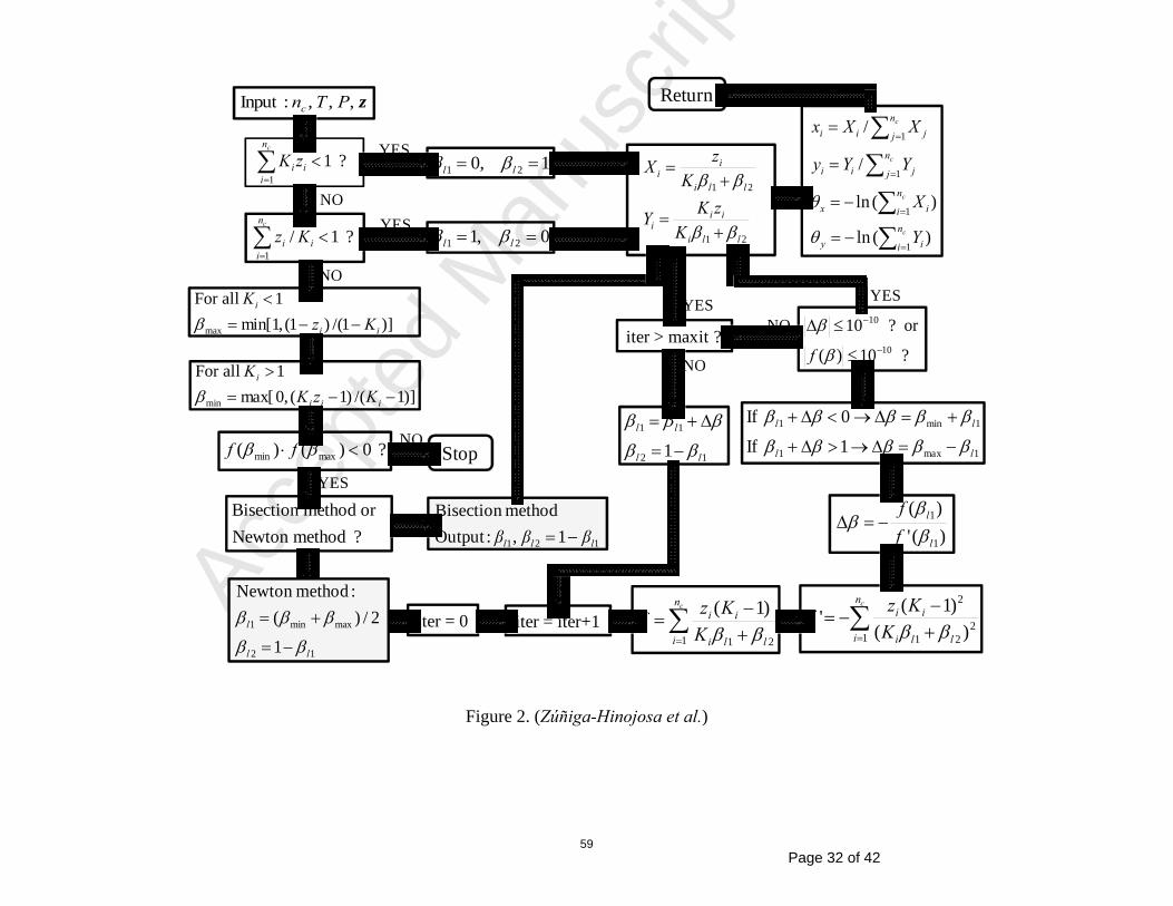
in, respectively, the feed, the first (light) liquid phase, and the second (dense) liquid phase. Fig. 2 shows
the algorithm for the Rachford-Rice flash calculation. It can be seen in this figure that a bisection method
(e.g., the Brent method [33]) can be used instead of Newton-Raphson method to improve convergence.
This is due to the very large K-values of the asphaltene fractions which, sometimes, makes difficult to
apply the Newton-Raphson method.
Equation (24) yields a physically correct root for 10 << β using constant K-values determined in an
outer loop. Once the value of β is determined, mole fractions of each component in every phase are
calculated from the relations
)1(1 −+=
i
ii K
zXβ
(25)
iii
iii KX
KKzY =
−+=
)1(1 β (26)
where iX and iY are non-normalized mole fractions and their summations ∑ =Ni iX1 and ∑ =
Ni iY1 are equal
to one when convergence is achieved.
In this algorithm, the K-values are updated in an outer loop after each iteration, since they depend on the
composition of each phase, which is not known before convergence.
The updating procedure in based on the equilibrium conditions
21 ˆˆ Li
Li ff = Ni ,...,1= (27)
where 1ˆ Lif and 2ˆ L
if are, respectively, the fugacities of component i at the first and second liquid phases,
and the convergence criteria that satisfies the stability test [34]
θ=− izi ff lnln Ni ,...,1= (28)
Page 11 of 42
Accep
ted
Man
uscr
ipt
38
where if is the fugacity of component i for a new potential phase and izf is the reference fugacity of
component i in all the existing phases. Equation (28) can be written as
⎟⎟⎠
⎞⎜⎜⎝
⎛=−=
iiz
iixizix z
xffφφθ lnlnln (29)
or
∑=
−=N
jjx X
1lnθ (30)
which is valid for any phase.
On the other hand, the method reported by Sabbagh [31] to establish the stability criteria at equilibrium is
given by
iyix ff = Ni ,...,1= (31)
or
pypx iiyiix φφ = Ni ,...,1= (32)
and the equilibrium ratios, which can be expressed as
iyi
ixi
iy
ix
i
ii fx
fyxyK ===
φφ Ni ,...,1= (33)
or
⎟⎟⎠
⎞⎜⎜⎝
⎛+⎟
⎟⎠
⎞⎜⎜⎝
⎛=
i
i
iy
ixi x
yffK lnlnln Ni ,...,1= (34)
where iX and iY are obtained from the solution of the Rachford-Rice, and ix and iy are their normalized
mole fractions. Consequently, Eq. (34) can also be written as
⎟⎟⎠
⎞⎜⎜⎝
⎛−−+−⎟⎟
⎠
⎞⎜⎜⎝
⎛= ∑∑
==
N
jjix
N
jjiy
i
ii XfYf
XYK
11lnlnlnlnlnln Ni ,...,1= (35)
or
[ ]xixyiyi
ii ff
XYK θθ +−−−⎟⎟
⎠
⎞⎜⎜⎝
⎛= lnlnlnln Ni ,...,1= (36)
If the equilibrium ratios iK at iteration k are defined as

Page 12 of 42
Accep
ted
Man
uscr
ipt
39
( ) )()( / kii
ki XYK = Ni ,...,1= (37)
then the equilibrium ratios iK at iteration )1( +k can be calculated as follows
ik
ik
i gKK −=+ )()1( lnln Ni ,...,1= (38)
where
xixyiyi ffg θθ +−−= lnln Ni ,...,1= (39)
Equation (38) is based on the successive substitution method, which has linear convergence rate. To
accelerate the convergence, a suitable step length γ can be used. In such a case, Eq. (38) is written as
ik
ik
i gKK γ−=+ )()1( lnln Ni ,...,1= (40)
where γ is set equal to unity at the start of calculations and it is modified using an appropriate numerical
method during the iteration process.
To use the procedure outlined above, the K-values must be initialized. This is done by first setting the K-
values of all components, except for the asphaltene fractions, to zero. Then, the K-values for the
asphaltene subfractions are initialized by assuming the mole fractions of the light liquid phase equal to the
mole fractions of feed components (except for the asphaltenes), and calculating the mole fractions of
components of the dense liquid phase from the molar masses and mass fractions of the asphaltene
fractions. The K-values are then calculated from the ratio of the asphaltene pseudo-components mole
fractions in the dense liquid phase to the mole fractions of the same pseudo-components in the light liquid
phase.
During the liquid-liquid flash calculation, the Rachford-Rice equation is solved for the moles of the dense
liquid phase by using the Newton-Raphson method or a bisection method to obtain convergence. After
convergence, the component mole fractions of each phase are calculated using the updated K-values and
the obtained moles of the dense liquid phase are used to calculate the mass of the dense liquid phase (the
precipitate) in order to determine the fractional yield of asphaltene precipitation, defined as the mass of
precipitated asphaltenes and solids divided by the mass of the heavy oil or bitumen [16]. In this
procedure, fugacities of the components in the two liquid phases were calculated with the PC-SAFT
equation of state.

Page 13 of 42
Accep
ted
Man
uscr
ipt
40
2.3 Determination of asphaltenes PC-SAFT parameters
The correlations reported in the literature for estimating the three pure-component parameters (i.e.,
number of segments per chain m , temperature-independent segment diameter σ , and depth of the
potential ε ) characterizing the PC-SAFT equation of state for asphaltenes, are valid for asphaltene
subfractions of molar masses up to 1475 g/mol [35]. However, these correlations cannot be used to
estimate such parameters for asphaltenes that can reach very high molar masses, e.g., 15,000 g/mol.
The use of the gamma distribution function to split the asphaltenes SARA fraction into subfractions
indicates that the first asphaltene subfraction −the one with the smallest molar mass of the subfractions–
should be greater than the monomer molar mass value. The molar masses of the different subfractions
were obtained from the difference between the largest molar mass (set to 15,000 g/mol) and the monomer
molar mass, divided by the number of subfractions; i.e., 30. For the heavy oils and bitumens studied here,
the monomer molar mass value was set to 1800 g/mol [16], All these molar mass values are beyond the
range of validity of the reported correlations to estimate the PC-SAFT parameters m , σ , and ε for
asphaltene subfractions.
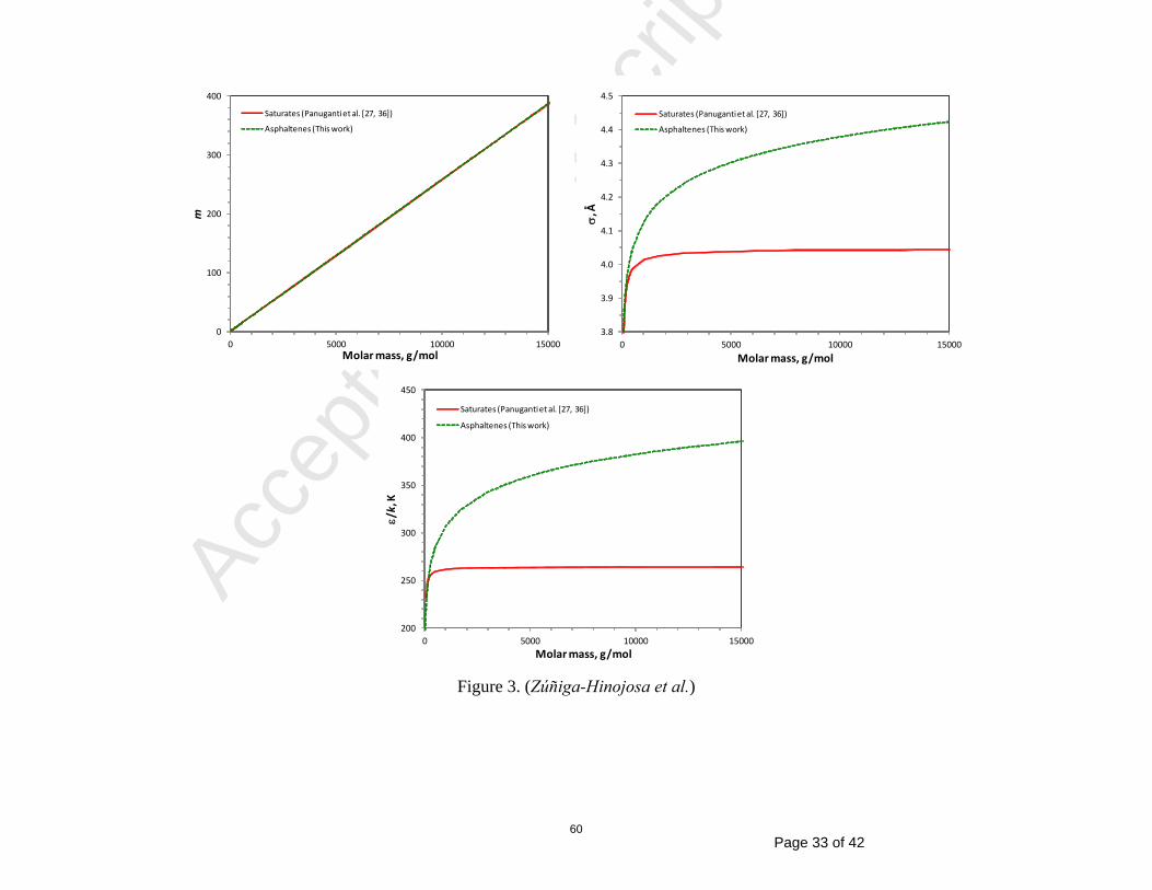
This aspect is illustrated in Fig. 3, which shows the PC-SAFT parameters m , σ , and k/ε for saturates
pseudo-component as a function of the molar mass calculated from the correlations reported by Panuganti
et al. [27,36]. As can be seen in this figure, parameters σ and k/ε tend to reach an asymptotic value as
the molar mass increases. If these correlations were used to calculate parameters σ and k/ε for the
asphaltene subfractions at molar masses greater than, say 2000 g/mol, all the subfractions would have
similar σ and k/ε values, which is not desired in practice. It is therefore necessary that parameters σ
and k/ε increase as the molar mass of the asphaltene subfraction increases.
To circumvent this problem, we suggest the following empirical correlations for estimating the PC-SAFT
parameters m , σ , and k/ε as a function of the molar mass of each asphaltene subfraction:
8444.00257.0 += Mm (41)
3685.3ln1097.0 += Mσ (42)
398.80ln81.32/ += Mkε (43)

Page 14 of 42
Accep
ted
Man
uscr
ipt
41
where M is the molar mass of the asphaltene subfraction, and parameters σ , and k/ε are given in units
of Å and Kelvin, respectively, whereas parameter m is dimensionless.
The correlations given by Eqs. (41)−(43) allow estimating the PC-SAFT parameters m , σ , and k/ε to
represent the several asphaltene subfractions resulting from the gamma distribution function. It should be
mentioned that these correlations were developed by assuming that the asphaltene subfractions behave as
long linear chains of carbons molecules. Of course, this does not correspond to the real structural form of
any asphaltenes fraction; however, it is just a “practical” way to conceive and approximate the structural
form of the asphaltenes to predict with the PC-SAFT model the complex phase behavior of the asphaltene
precipitation process experimentally exhibited from n-alkane diluted heavy oils and bitumens.
Table 1 presents the PC-SAFT parameters m , σ , and k/ε calculated from correlations (41)−(43) for the
“hypothetical” asphaltene subfractions used in this work. These parameters are also plotted in Fig. 3. This
figure shows that, according to correlations (41)−(43), parameter m increases linearly as the molar mass
increases, while parameters σ and k/ε increase in a regular trend as the molar mass increases without
reaching an asymptotic value.
On the other hand, because the saturates, aromatics, and resins fractions obtained from the SARA analysis
are considered to be pseudo-components with molar masses not greater than 1100 g/mol for the heavy
oils and bitumens studied, it seems reasonable to use the correlations suggested by Panuganti et al. [27,
36] to estimate the PC-SAFT parameters m , σ , and k/ε for these pseudo-components. That is, the
following correlations were used
8444.00257.0 += Mm (44)
MM /)ln8013.4(047.4 −=σ (45)
)/523.95769.5exp(/ Mk −=ε (46)
for saturates pseudo-component, and
)7296.10101.0()751.00223.0()1( +++−= MMm γγ (47)
)/98.936169.4()/1483.381377.4()1( MM −+−−= γγσ (48)
)/234100508()93.28300436.0()1(/ MMk −++−= γγε (49)

Page 15 of 42
Accep
ted
Man
uscr
ipt
42
for aromatics + resins pseudo-component, where γ is the degree of aromaticity that determine the
tendency of the aromatics + resins pseudo-component to behave as a poly-nuclear aromatic )1( =γ or as
a benzene derivative component )0( =γ [37]. Here, it is assumed that the heavy oils and bitumens have a
low degree of aromaticity, so that we set the aromaticity factor γ to 0.01 to estimate the PC-SAFT
parameters m , σ , and k/ε for aromatics and resins pseudo-components.
Fig. 4 shows the calculated m , σ , and k/ε parameters for saturates, aromatics, and resins pseudo-
components as a function of the molar mass. The PC-SAFT parameters for aromatics and resins pseudo-
components were calculated (1) by assuming that the resins pseudo-component behaves as a poly-nuclear
aromatic and the aromatics pseudo-component as a benzene derivative component (solid lines), and (2)
by using an aromaticity factor of 0.01 (dashed lines). This figure also shows the PC-SAFT parameters for
asphaltenes calculated from correlations (41)−(43). Also showed in this figure are the calculated PC-
SAFT parameters for saturates, aromatics, and resins fractions with corresponding molar masses of 460,
522, and 1040 g/mol (solid square symbols) [16] by using an aromaticity factor of 0..01 for the aromatics
and resins pseudo-components.
3.4 Estimation of interaction parameters
It is typical in equation of state calculations to introduce binary interactions (BIPs) for modeling the phase
behavior of complex systems such as exhibited by the system heavy oil (or bitumen)-solvent. In this case,
the BIPs are used between the heaviest most polar component (asphaltenes) and the lightest, least polar
component (the n-alkane). The interaction parameters between different asphaltene subfractions are set to
zero, and they are considered to have similar structures. The BIPs between asphaltenes and n-alkane are
assumed to be the same for all the asphaltene subfractions. Thus, the only interaction parameter used in
the modeling is the one corresponding to the interaction between asphaltene and n-alkane. All other
interactions parameters between asphaltenes + saturates, asphaltenes + aromatics, asphaltenes + resins,
saturates + aromatics, saturates + resins, and aromatics + resins pseudo-components, aromatics + n-
alkanes, and resins + n-alkanes, are set to zero.
The BIPs are generally determined by minimizing the difference between the model predictions and the
experimental data. Therefore, to increase the usefulness of the combining rule given in Eq. (13), we have
determined the binary interaction parameter ijk characterizing the interactions between the asphaltene

Page 16 of 42
Accep
ted
Man
uscr
ipt
43
subfractions and the n-alkane for the PC-SAFT equation of state by minimizing the difference between
the experimental fractional yields (amount of precipitated asphaltene) and those ones calculated with the
PC-SAFT model for different concentrations of n-alkane.
The simplex optimization procedure of Nelder and Mead [38] was used in the computations by searching
the minimum of the following objective function
∑=
⎟⎟⎠
⎞⎜⎜⎝
⎛ −=
M
iexp
i
cali
expi
obj YYYF
1
2
(50)
where )( cali
expi YY − is the difference between the experimental and calculated values of fractional yields
for an experiment i , and M is the total number of experimental data.
In a first attempt, we used all the asphaltene fractional yield data reported by Sabbagh et al. [16] to obtain
a single binary interaction for each bitumen or heavy oil, independent of temperature or composition.
However, we found a rather poor agreement between the experimental fractional yields and those values
calculated with the PC-SAFT model, so that we realized than a single interaction parameter was not
enough to give a good representation of the experimental fractional yield data for any of the seven n-
alkane diluted bitumens and heavy oils investigated in this work. Therefore, to follow the behavior of
these interaction parameters as a function of the n-alkane mass fraction, we adjusted the interaction
parameter for each fractional yield datum (i.e., 1=M ). This is illustrated in Figs. 5 and 6.
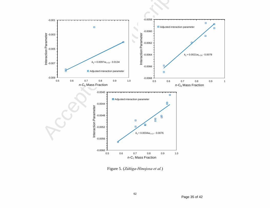
Fig. 5 shows the behavior of the interaction parameter as a function of the n-alkane mass fraction from
the Athabasca bitumen diluted with n-pentane, n-hexane, and n-heptane at 296.2 K and 0.1 MPa. This
figure shows that all the interaction parameters are negative but they become less negative as the
concentration of the n-alkane increases. In this case, the interaction parameter values varied from (−0.008
to −0.002), (−0.0067 to −0.0057), and (−0.0057 to −0.0041), for n-pentane, n-hexane, and n-heptane,
respectively.
Fig. 5 also shows that there exists a great deal of scatter among the adjusted interaction parameters, may
be due to possible experimental errors in the method of determining the asphaltene fractional yields.
Notwithstanding this fact, they were correlated to the following straight line
bwak alknij +⋅= − (51)

Page 17 of 42
Accep
ted
Man
uscr
ipt
44
where ijk is the binary interaction parameter between asphaltenes and the n-alkane and it is assumed that
they are the same for all the asphaltene subfractions, alknw − is the n-alkane mass fraction, and a and b
are the two constants of the correlation. Although the values of the interaction parameters are in general
small, they are very sensitive when these are used to calculate the fractional yield at a given n-alkane
composition, as will be discussed below.
Fig. 6 shows the behavior of the interaction parameter as a function of the n-alkane mass fraction from
the Athabasca bitumen diluted with n-heptane at 273.2 and 0.1 MPa, and at 296.2, 323.2, and 373.2 K all
at 2.1 MPa. This figure shows the effect of temperature and pressure upon the behavior of the interaction
parameters as a function of the n-heptane. As seen in this figure, the interaction parameters are negative at
the lower temperatures, irrespective of the pressure, varying from (−0.0095 to −0.0059) and (−0.0061 to
−0.0042) as the n-alkane concentration increases, similar to those showed in Fig. 5. However, as
temperature increases, the slope of the straight line changes from positive to negative. That is, the
interaction parameters varying from (−0.0013 to −0.0030) and (0.0020 to −0.0024) at 323.2 and 373.2 K
both at 2.1 MPa, respectively, as the n-alkane concentration increases. This indicates that the influence of
temperature is stronger than pressure when correlating the fractional yield data for this bitumen diluted
with n-heptane. The same behavior is observed for the Cold Lake bitumen diluted with n-heptane at 296.2
and 323. 2 K both at 2.1 MPa, and at 373.2 K and 6.9 MPa
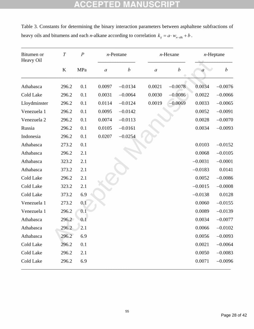
Table 3 presents the estimated constants a and b of the linear correlations to calculate the interaction
parameters for asphaltene−n-alkane interactions of Athabasca, Cold Lake, Lloydminster, Venezuela 1,
Venezuela 2, Russia and Indonesia bitumens and heavy oils, where the n-alkane is either n-pentane, or n-
hexane, or n-heptane. They are listed according to Figs. 9−20 presented in Sabbagh et al.’s article [16].
4. Modeling results and discussion
To investigate the ability of the PC-SAFT equation of state to predict asphaltene precipitation, the
procedure suggested by Sabbagh et al. [16] was used for calculating asphaltene fractional yields of
Athabasca, Cold Lake, Lloydminster, Venezuela 1, Venezuela 2, Russia and Indonesia bitumens and
heavy oils diluted with n-alkanes. In all the calculations, the PC-SAFT equation of state was used as the
thermodynamic model to represent the liquid phases in conjunction with interaction parameters estimated
from Eq. (51). The characteristic parameters m , σ , and k/ε for saturates, aromatics and resins pseudo-

Page 18 of 42
Accep
ted
Man
uscr
ipt
45
components, and for asphaltene subfractions, are given in Table 1, while those corresponding to the
precipitating compounds (n-pentane, n-hexane, and n-heptane) were taken from Gross and Sadowski [28].
SARA analysis fractions (in weight %) and asphaltene average associated molar masses for the seven
bitumens and heavy oils studied in this work are given in Table 2. The average molar mass reported by
Sabbagh et al. for each SARA fraction are 460, 522, 1040, and 1800 g/mol for saturates, aromatics,
resins, and asphaltenes (monomer), respectively. Results from the modeling of the bitumens and heavy
oils diluted with an n-alkane (n-pentane, or n-hexane, or n-heptane) at several conditions of temperature
and pressure, are given below.
4.1 n-Alkane diluted heavy oils and bitumens
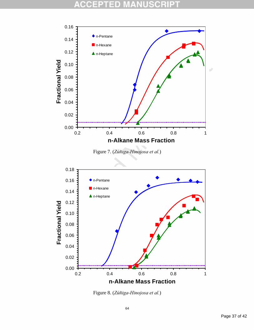
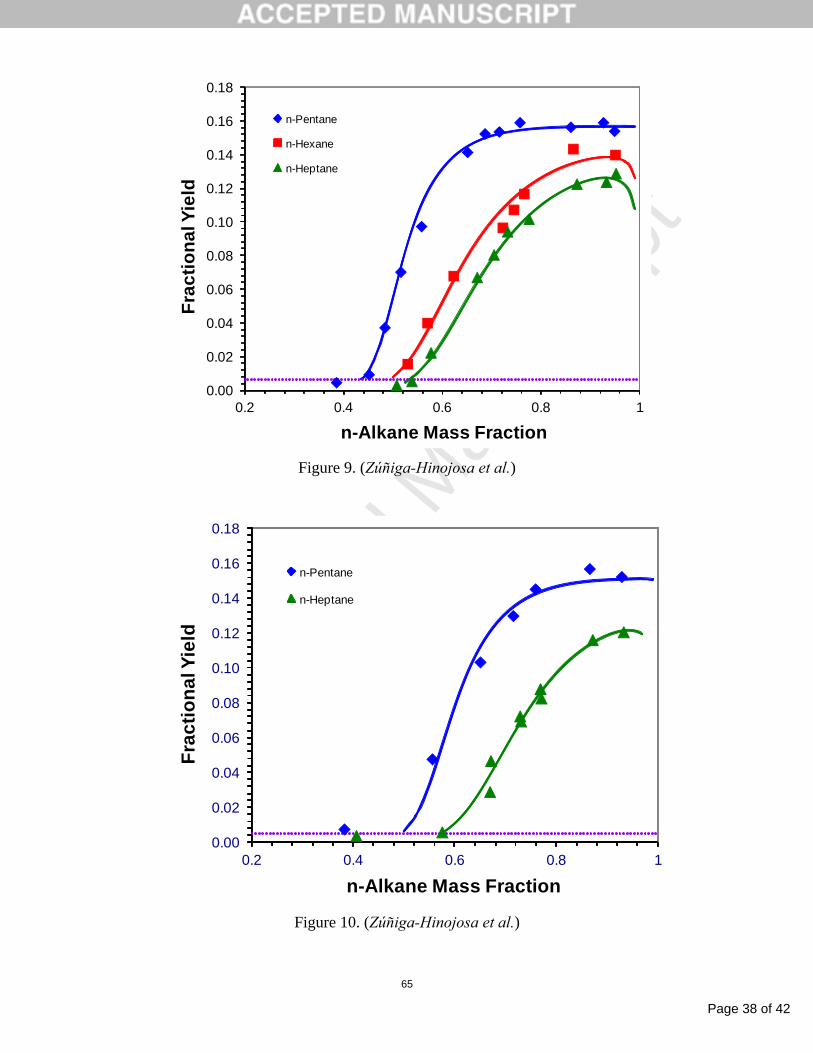
Figs. 7�13 show the measured asphaltene fractional yields from Athabasca, Cold Lake, Lloydminster,
Venezuela 1, Venezuela 2, Russia and Indonesia bitumens and heavy oils diluted with n-alkanes (n-
pentane, n-hexane, and n-heptane) at 296.2 K and atmospheric pressure, and those ones calculated with
the PC-SAFT equation of state at the same conditions of temperature and pressure. As seen in these
figures, the calculated fractional yields are in good agreement with the experimental ones when they are
calculated using interaction parameters that depend on the n-alkane mass fraction as given by Eq. (51).
By using the PR equation of state [17] with interaction parameters between asphaltene subfractions and
the n-alkane, independents of temperature and n-alkane concentration, Sabbagh et al. [16] obtained a
reasonable representation of the asphaltene fractional yields for these heavy oils and bitumens diluted
with n-pentane, n-hexane and n-heptane. However, the representation of the asphaltene fractional yields
for the heavy oils and bitumens diluted with n-pentane was rather poor. Although, they claim that, in most
cases, the average absolute deviation was less than 0.02 (fractional yield) and that the greatest
discrepancies occurred at high n-pentane mass fractions, possibly due to that (1) the model did not
account for the partition of the resins to the dense phase, (2) there was a significant mass of trapped
maltenes (i.e., saturates, aromatics, and resins) at the high fractional yields measured in n-pentane, and (3)
the formation of multiple liquid and/or solid phases that were not accounted for in the modeling, it is clear
that a single interaction parameter independent of temperature and solvent concentration is not enough to
adequately represent the experimental data of asphaltene precipitation irrespective of the equation of state
used, as shown in Figs. 5 and 6. Of course, it is also possible that these discrepancies may be due to errors
in the experimental data as pointed out by Sabbagh et al.
Page 19 of 42
Accep
ted
Man
uscr
ipt
46
Similar results were obtained by Li and Firoozabadi [25] when they modeled the asphaltene precipitation
for the same heavy oils and bitumens using the CPA equation of state [24]. They characterized the heavy
oils and bitumens in terms of saturates, aromatics/resins, and asphaltenes. In this model, the physical
interactions were described by the PR equation of state [17] and the self-association between asphaltenes
and aromatics/resins were represented by the thermodynamic perturbation theory of Wertheim [39-42].
The model contains only one adjustable parameter, namely, the cross energy between asphaltenes and
aromatics/resins molecules that depends on the types of asphaltenes and n-alkane, and probably
temperature, but is independent of pressure and n-alkane concentration. Through the adjustment of this
parameter, they reproduced most of the experimental fractional yield data. However, for n-pentane at high
mass fractions, the fractional yield was always underestimated, in spite of considering in their model the
partitioning of resins to the dense liquid phase rich in asphaltenes.
Figs. 7−13 also show that the PC-SAFT predictions of the fractional yields for both low and high n-
pentane concentrations are in very good agreement with the experimental data and that the discrepancies
existing between the experimental and calculated fractional yields may be due to experimental errors and
not to the ability of the equation of state in modeling this type of systems.
The PC-SAFT equation of state has also successfully been used to modeling the asphaltene precipitation
process of several n-alkane diluted Mexican oils and their blends at 296.2 K and atmospheric pressure,
which experimentally exhibit a large region of “colloidal stability” as a function of the n-alkane mass
fraction. This wide region both limits and delays the asphaltene precipitation process. The results of the
modeling will be presented in a subsequent communication.
4.2 n-Alkane diluted heavy oils and bitumens as a function of temperature
Figs. 14−16 show the effect of temperature on the experimental and calculated asphaltene fractional
yields from Athabasca and Cold Lake bitumens diluted with n-heptane, and from Venezuela 1 heavy oil
diluted with n-pentane, respectively. Fig. 14 presents the results of the modeling obtained with the PC-
SAFT equation of state at 273.2 K and 0.1 MPa, and at 296.2, 323.2 and 373.2 K all at 2.1 MPa, whereas
Fig. 15 shows the results of the modeling realized at 296.2 and 323.2 K both at 2.1 MPa, and 373.2 K and
6.9 MPa. These figures show, in general, that there exists a good agreement between the experimental and
Page 20 of 42
Accep
ted
Man
uscr
ipt
47
calculated asphaltene fractional yields, except at 373.2 K where the representation of the experimental
data is rather poor, may be due to some experimental difficulties to obtain consistent data at this
temperature, as pointed out by Sabbagh et al. [16]. These figures also show that the asphaltene fractional
yield decreases as temperature increases, irrespective of the pressure.
Fig. 16 presents the results of the modeling at 273.2 and 296.2 K both at 0.1 MPa. An examination of this
figure shows that there is a poor agreement between the experimental and calculated asphaltene fractional
yields for the two sets of experimental data. These discrepancies are due to that the adjusted interaction
parameters do not follow a linear trend in function of the n-pentane mass fraction, so that it was not
possible to obtain a suitable linear correlation from these interaction parameters. For instance, the
adjusted interaction parameter at 296.2 K, which correctly matches the experimental asphaltene fractional
yield, was −0.00713 for an n-pentane mass fraction of 0.3832, but this interaction parameter becomes
more negative as the n-pentane mass fraction increases up to reach a value of about 0.6. Then, the
interaction parameters turn back to be less negative as the n-pentane mass fraction increases reaching a
value of −0.00557 at an n-pentane mass fraction of 0.9267. Consequently, the interaction parameter
estimated from the linear correlation given by Eq. (51) was not able to correctly predict the asphaltene
fractional yield at the n-pentane mass fraction of 0.3832, as can be seen in this figure. This example
illustrates the strong effect of the interaction parameters in predicting the asphaltene precipitation for the
heavy oils and bitumens studied in this work.
4.3 n-Alkane diluted heavy oils and bitumens as a function of pressure
Figs. 17−18 show the effect of pressure on the experimental and calculated asphaltene fractional yields
from the Athabasca and Cold Lake bitumens, respectively, diluted with n-heptane at 296.2 K and
pressures of 0.1, 2.1, and 6.9 MPa. These figures show that the asphaltene fractional yields obtained with
the PC-SAFT equation of state are, on the whole, in good agreement with the experimental data for both
bitumens diluted with n-heptane. Also observed in these figures is the little effect of pressure on the
experimental and calculated asphaltene fractional yields; the experimental and calculated fractional yields
decrease only slightly with pressure for both bitumens. This indicates that the effect of temperature on the
asphaltene fractional yields is stronger than the effect of pressure.
Page 21 of 42
Accep
ted
Man
uscr
ipt
48
Finally, it is worth mentioning that the modeling results of asphaltene precipitation show a decrease in the
amount of precipitated asphaltene at high n-alkane fractions (high dilution) for most of the figures
presented above (see Figs. 7-18), whereas the experimental data points follow a different trend. As can be
seen in these figures, the PC-SAFT EoS is able to give good results both for the onset point at which the
precipitation begins and for the fractional yields at different n-alkane mass fractions (usually less than
0.9). These figures also show that at high n-alkane mass fractions, the model predicts a maximum in the
fractional yield, but at higher n-alkane mass fractions a decrease in the precipitated asphaltene is
observed. An explanation of this behavior is that, in thermodynamic models, the asphaltenes have a small
solubility in n-alkanes. However, at very high n-alkane mass fractions, the concentration of asphaltenes in
the system is very small and the small amount that remains soluble reduces the amount of precipitated
asphaltene, so that the decreasing in the fractional yield is a result of dilution effects that become
dominant.
5. Conclusions
The ability of the PC-SAFT thermodynamic model to predict the asphaltene precipitation process
obtained by the addition of an n-alkane to seven bitumens and heavy oils at different conditions of
temperature and pressure was investigated. The results obtained showed that this equation of state is able
to satisfactorily represent the precipitation process of the asphaltenes for these bitumens and heavy oils by
using linear correlations for the binary interaction parameters of asphaltene (subfractions)−n-alkane as a
function of the n-alkane mass fraction.
Liquid-liquid equilibrium was assumed between a dense liquid phase (asphaltene-rich phase), which only
asphaltenes were allowed to partition, and a light liquid phase. The calculated fractional yields showed to
be very sensitive to the interaction parameter value. The heavy oils and bitumens were characterized in
terms of saturates, aromatics, resins, and asphaltenes fractions. The saturates, aromatics, and resins
fractions were considered as single pseudocomponents, whereas the asphaltenes fraction was divided into
subfractions of different molar mass based on a gamma distribution function. The use of a gamma
distribution function considering the self-aggregation of the asphaltenes through the average associated
molar mass, proved to be suitable for representing the molar mass distribution of the asphaltene
subfractions for the PC-SAFT equation of state.

Page 22 of 42
Accep
ted
Man
uscr
ipt
49
Acknowledgments
The authors thank the financial support of the Sectorial Fund CONACyT-SENER (Hydrocarbons) under
Project Y.00118. D. N. Justo-García gratefully acknowledges the National Polytechnic Institute for their
financial support through the Project SIP-20130658. M. A. Zúñiga-Hinojosa thanks the National Council
for Science and Technology of Mexico (CONACyT) and the Mexican Petroleum Institute for their
pecuniary support through a Ph.D. fellowship.
References
[1] A. K. Tharanivasan, W. Y. Svrcek, H. W. Yarranton, S. D. Taylor, D. Merino-Garcia, P. M. Rahimi. Energy Fuels 23 (2009) 3971−3980.
[2] A. Hirschberg, L. N. J. deJong, B. A. Schipper, J. G. Meijer. Soc. Pet. Eng. J. 24 (1984) 283−293.
[3] H. Alboudwarej, K. Akbarzadeh, J. Beck, W. Y. Svrcek, H. W. Yarranton. AIChE J. 49 (2003) 2948−2956.
[4] K. Akbarzadeh, H. Alboudwarej, W. Y. Svrcek, H. W: Yarranton. Fluid Phase Equilib. 232 (2005) 159−170.
[5] S. I. Andersen. Pet. Sci. Technol. 12 (1984) 1551−1577.
[6] H. W. Yarranton, J. H. Masliyah. AIChE J. 42 (1996) 3533−3543.
[7] J. S. Buckley, J. Wang, J. L. Creek. In: Asphaltenes, Heavy Oils, and Petroleomics, O. C. Mullins, E. Y. Sheu, A. Hammami, Eds., Springer Publishing, New York, pp. 401−437, 2007.
[8] K. J. Leontaritis, G. A. Mansoori. Paper SPE 16258 presented at the 1987 SPE Intl. Symposium on Oilfield Chemistry, San Antonio, Texas, 4-6 February, 1987.
[9] A. I. Victorov, A. Firoozabadi. AIChE J. 42 (1996) 1753−1764.
[10] H. Pan, A. Firoozabadi. SPE Production & Facilities 13 (1998) 118−127.
[11] A. I. Victorov, N. A. Smirnova. Fluid Phase Equilib. 158-160 (1999) 471−480.
[12] A. K. Gupta. M. Sc. Thesis, University of Calgary, Calgary, Alberta, Canada, 1986.
[13] L. X. Nghiem, M. S. Hassam, R. Nutakki, A. E. D. George. Paper SPE 26642 presented at the 68th Annual Technical Conference and Exhibition of the Society of Petroleum Engineers, Houston, Texas, 3-6 October 1993.
[14] L. X. Nghiem, D. A. Coombe. SPE J. 2 (1997) 170−176.
[15] B. F. Khose, L. X. Nghiem, H. Maeda, K. Ohno. Paper SPE 64465 presented at the SPE Asia Pacific Oil and Gas Conference and Exhibition, Brisbane, Australia, 16–18 October 2000.

Page 23 of 42
Accep
ted
Man
uscr
ipt
50
[16] O. Sabbagh, K. Akbarzadeh, A. Badamchi-Zadeh, W. Y. Svrcek, H. W. Yarranton. Energy Fuels 20 (2006) 625−634.
[17] D.-Y. Peng, D. B. Robinson. Ind. Eng. Chem. Fundam. 15 (1976) 59−64.
[18] P. D. Ting, G. J. Hirasaki, W. G. Chapman. Pet. Sci. Technol. 21 (2003) 647−661.
[19] W. G. Chapman, K. E. Gubbins, G. Jackson, M. Radosz. Ind. Eng. Chem. Res. 29 (1990) 1709− 1721.
[20] J. Wu, J. M. Prausnitz, A. Firoozabadi. AIChE J. 44 (1998) 1188−1199.
[21] J. Wu, J. M. Prausnitz, A. Firoozabadi. AIChE J. 46 (2000) 197−209.
[22] E. Buenrostro-Gonzalez, C. Lira-Galeana, A. Gil-Villegas, J. Wu. AIChE J. 50 (2004) 2552−2570.
[23] A. Gil-Villegas, A. Galindo, P. J. Whitehead, S. Mills, G. Jackson. J. Chem. Phys. 106 (1997) 4168−4186.
[24] G. M. Kontogeorgis, E. C. Voutsas, I. V. Yakoumis, D. P. Tassios. Ind Eng. Chem. Res. 35 (1996) 4310−4318.
[25] Z. Li, A. Firoozabadi. Energy Fuels 24 (2010) 1106−1113.
[26] Z. Li, A. Firoozabadi. Energy Fuels 24 (2010) 2956−2963.
[27] S. R. Panuganti, F. M. Vargas, D. L. Gonzalez, A. S. Kurup, W. G. Chapman. Fuel 93 (2012) 658−669.
[28] J. Gross, G. Sadowski. Ind. Eng. Chem. Res. 40 (2001) 1244−1260.
[29] S. S. Chen, A. Kreglewski. Ber. Bunsenges. Phys. Chem. 81(1977) 1048−1052.
[30] K. Akbarzadeh, A. Dhillon, W. Y. Svrcek, H. W. Yarranton. Energy Fuels 18 (2004) 1424−1441.
[31] O. Sabbagh. M.Sc. Thesis, University of Calgary, Calgary, Alberta, Canada, 2004.
[32] H. H. Rachford, J. D. Rice. Petrol. Trans. AIME 195 (1952) 327−328.
[33] W. H. Press, S. A. Teukolsky, W. T. Vetterling, B. P. Flannery. Numerical Recipes in Fortran: The Art of Scientific Computing, 2nd ed., Cambridge University Press, New York, 1992.
[34] R. A. Heidemann, M. L. Michelsen. Ind. Eng. Chem. Res. 34 (1995) 958−966.
[35] M. Tavakkoli, S. R. Panuganti, V. Taghikhani, M. R. Pishvaie, W. G. Chapman. Fuel 117 (2014) 206−217.
[36] S. R. Panuganti, M. Tavakkoli, F. M. Vargas, D. L. Gonzalez, W. G. Chapman. Fluid Phase Equilib. 359 (2013) 2−16.
[37] D. L. Gonzalez, G. J. Hirasaki, W. G. Chapman. Energy Fuels 21 (2007) 1231−1242.
[38] J. A. Nelder, R. A. Mead. Comput. J. 7 (1965) 308−313.
[39] M. S. Wertheim. J. Stat. Phys. 35 (1984) 19−34.
[40] M. S. Wertheim. J. Stat. Phys. 35 (1984) 35−47.
Page 24 of 42
Accep
ted
Man
uscr
ipt
51
[41] M. S. Wertheim. J. Stat. Phys. 42 (1986) 459−476.
[42] M. S. Wertheim. J. Stat. Phys. 42 (1986) 477−492.

Page 25 of 42
Accep
ted
Man
uscr
ipt
52
Table 1. PC-SAFT parameters for saturates, aromatics, and resins pseudo-components, a and asphaltene subfractions. b _________________________________________________________
Component M m σ k/ε g/mol Å K _________________________________________________________ Saturates 460.0 12.6664 3.9830 258.84 Aromatics 522.0 12.3377 4.0683 288.23 Resins 1040.0 23.8259 4.1053 290.59 Asph. subfract. 1 2191.6 57.1696 4.2124 332.79 Asph. subfract. 2 2569.4 66.8784 4.2298 338.00 Asph. subfract. 3 2956.6 76.8296 4.2452 342.61 Asph. subfract. 4 3364.8 87.3189 4.2594 346.85 Asph. subfract. 5 3785.5 98.1314 4.2723 350.72 Asph. subfract. 6 4213.0 109.1177 4.2840 354.23 Asph. subfract. 7 4644.3 120.2028 4.2947 357.43 Asph. subfract. 8 5078.0 131.3484 4.3045 360.35 Asph. subfract. 9 5513.2 142.5331 4.3136 363.05 Asph. subfract. 10 5949.4 153.7445 4.3219 365.55 Asph. subfract. 11 6385.4 164.9749 4.3297 367.88 Asph. subfract. 12 6823.9 176.2193 4.3370 370.05 Asph. subfract. 13 7261.9 187.4741 4.3438 372.09 Asph. subfract. 14 7700.1 198.7371 4.3502 374.01 Asph. subfract. 15 8138.6 210.0065 4.3563 375.83 Asph. subfract. 16 8577.3 221.2810 4.3620 377.55 Asph. subfract. 17 9016.2 232.5598 4.3675 379.19 Asph. subfract. 18 9455.2 243.8419 4.3727 380.75 Asph. subfract. 19 9894.3 255.1269 4.3777 382.24 Asph. subfract. 20 10333.5 266.4144 4.3825 383.67 Asph. subfract. 21 10772.7 277.7039 4.3870 385.03 Asph. subfract. 22 11212.1 288.9952 4.3914 386.34 Asph. subfract. 23 11651.5 300.2880 4.3956 387.60 Asph. subfract. 24 12091.0 311.5821 4.3997 388.82 Asph. subfract. 25 12530.5 322.8774 4.4036 389.99 Asph. subfract. 26 12970.0 334.1737 4.4074 391.12 Asph. subfract. 27 13409.6 345.4709 4.4111 392.22 Asph. subfract. 28 13849.2 356.7689 4.4146 393.27 Asph. subfract. 29 14288.8 368.0676 4.4180 394.30 Asph. subfract. 30 14728.5 379.3670 4.4214 395.29 _________________________________________________________
Page 26 of 42
Accep
ted
Man
uscr
ipt
53
a Calculated from Panuganti et al.’s correlations [27, 36]. b Calculated from correlations (41)−(43).

Page 27 of 42
Accep
ted
Man
uscr
ipt
54
Table 2. SARA analysis (wt %) of heavy oils and bitumens, a asphaltene average associated molar mass a
)(M , and average aggregation number )(r .
_____________________________________________________________________________________
Bitumen or Saturates Aromatics Resins Asphaltenes Solids M r Heavy Oil g/mol _____________________________________________________________________________________
Athabasca 16.3 39.8 28.5 14.6 0.8 4200 2.33 Cold Lake 19.4 38.1 26.7 15.3 0.5 4050 2.25 Lloydminster 23.1 41.7 19.5 15.1 0.6 4000 2.22 Venezuela 1 15.4 44.4 25.0 15.0 0.2 4290 2.38 Venezuela 2 20.5 38.0 19.6 21.8 0.1 4290 2.38 Russia 25.0 31.1 37.1 6.8 0.0 4800 2.67 Indonesia 23.2 33.9 38.2 4.7 0.0 3960 2.20 ____________________________________________________________________________________ a Ref. [16].
Page 28 of 42
Accep
ted
Man
uscr
ipt
55
Table 3. Constants for determining the binary interaction parameters between asphaltene subfractions of
heavy oils and bitumens and each n-alkane according to correlation bwak nij +⋅= −alk .
_____________________________________________________________________________________
Bitumen or T P n-Pentane n-Hexane n-Heptane Heavy Oil _______________ _______________ _______________
K MPa a b a b a b _____________________________________________________________________________________
Athabasca 296.2 0.1 0.0097 −0.0134 0.0021 −0.0078 0.0034 −0.0076
Cold Lake 296.2 0.1 0.0031 −0.0064 0.0030 −0.0086 0.0022 −0.0066
Lloydminster 296.2 0.1 0.0114 −0.0124 0.0019 −0.0069 0.0033 −0.0065
Venezuela 1 296.2 0.1 0.0095 −0.0142 0.0052 −0.0091
Venezuela 2 296.2 0.1 0.0074 −0.0113 0.0028 −0.0070
Russia 296.2 0.1 0.0105 −0.0161 0.0034 −0.0093
Indonesia 296.2 0.1 0.0207 −0.0254
Athabasca 273.2 0.1 0.0103 −0.0152
Athabasca 296.2 2.1 0.0068 −0.0105
Athabasca 323.2 2.1 −0.0031 −0.0001
Athabasca 373.2 2.1 −0.0183 0.0141
Cold Lake 296.2 2.1 0.0052 −0.0086
Cold Lake 323.2 2.1 −0.0015 −0.0008
Cold Lake 373.2 6.9 −0.0138 0.0128
Venezuela 1 273.2 0.1 0.0060 −0.0155
Venezuela 1 296.2 0.1 0.0089 −0.0139
Athabasca 296.2 0.1 0.0034 −0.0077
Athabasca 296.2 2.1 0.0066 −0.0102
Athabasca 296.2 6.9 0.0056 −0.0093
Cold Lake 296.2 0.1 0.0021 −0.0064
Cold Lake 296.2 2.1 0.0050 −0.0083
Cold Lake 296.2 6.9 0.0071 −0.0096 ____________________________________________________________________________________
Page 29 of 42
Accep
ted
Man
uscr
ipt
56
FIGURE CAPTIONS
Fig. 1. Flow diagram to calculate liquid-liquid equilibrium for asphaltene precipitation (adapted from Sabbagh [31]).
Fig. 2. Flow diagram for Rachford-Rice flash calculation (adapted from Sabbagh [31]). Fig. 3. PC-SAFT parameters m , σ , and k/ε as a function of molar mass for saturates pseudo-
component and asphaltene subfractions. Fig. 4 PC-SAFT parameters m , σ , and k/ε as a function of molar mass for saturates, aromatics, and
resins pseudo-components, and asphaltene subfractions. Fig. 5. Binary interaction parameters as a function of n-alkane mass fraction from Athabasca bitumen
diluted with n-alkanes at 296.2 K and 0.1 MPa. Fig. 6. Binary interaction parameters as a function of n-alkane mass fraction from Athabasca bitumen
diluted with n-heptane at 273.2 K and 0.1 MPa, and at 296.2, 323.2 and 373.2 K all at 2,1 MPa. Fig. 7. Experimental and calculated fractional yield from Athabasca bitumen diluted with n-alkanes at
296.2 K and 0.1 MPa. Symbols are experimental data from Sabbagh et al. [16], solid lines are calculated fractional yields with the PC-SAFT EoS, and dotted line is the solids content.
Fig. 8. Experimental and calculated fractional yield from Cold Lake bitumen diluted with n-alkanes at
296.2 K and 0.1 MPa. Symbols are experimental data from Sabbagh et al. [16], solid lines are calculated fractional yields with the PC-SAFT EoS, and dotted line is the solids content.
Fig. 9. Experimental and calculated fractional yield from Lloydminster heavy oil diluted with n-alkanes
at 296.2 K and 0.1 MPa. Symbols are experimental data from Sabbagh et al. [16], solid lines are calculated fractional yields with the PC-SAFT EoS, and dotted line is the solids content.
Fig. 10. Experimental and calculated fractional yield from Venezuela 1 heavy oil diluted with n-alkanes
at 296.2 K and 0.1 MPa. Symbols are experimental data from Sabbagh et al. [16], solid lines are calculated fractional yields with the PC-SAFT EoS, and dotted line is the solids content.
Fig. 11. Experimental and calculated fractional yield from Venezuela 2 heavy oil diluted with n-alkanes
at 296.2 K and 0.1 MPa. Symbols are experimental data from Sabbagh et al. [16], solid lines are calculated fractional yields with the PC-SAFT EoS, and dotted line is the solids content.
Fig. 12. Experimental and calculated fractional yield from Russia bitumen diluted with n-alkanes at
296.2 K and 0.1 MPa. Symbols are experimental data from Sabbagh et al. [16], solid lines are calculated fractional yields with the PC-SAFT EoS, and dotted line is the solids content.
Fig. 13. Experimental and calculated fractional yield from Indonesia bitumen diluted with n-pentane at
296.2 K and 0.1 MPa. Symbols are experimental data from Sabbagh et al. [16], solid lines are calculated fractional yields with the PC-SAFT EoS, and dotted line is the solids content.
Page 30 of 42
Accep
ted
Man
uscr
ipt
57
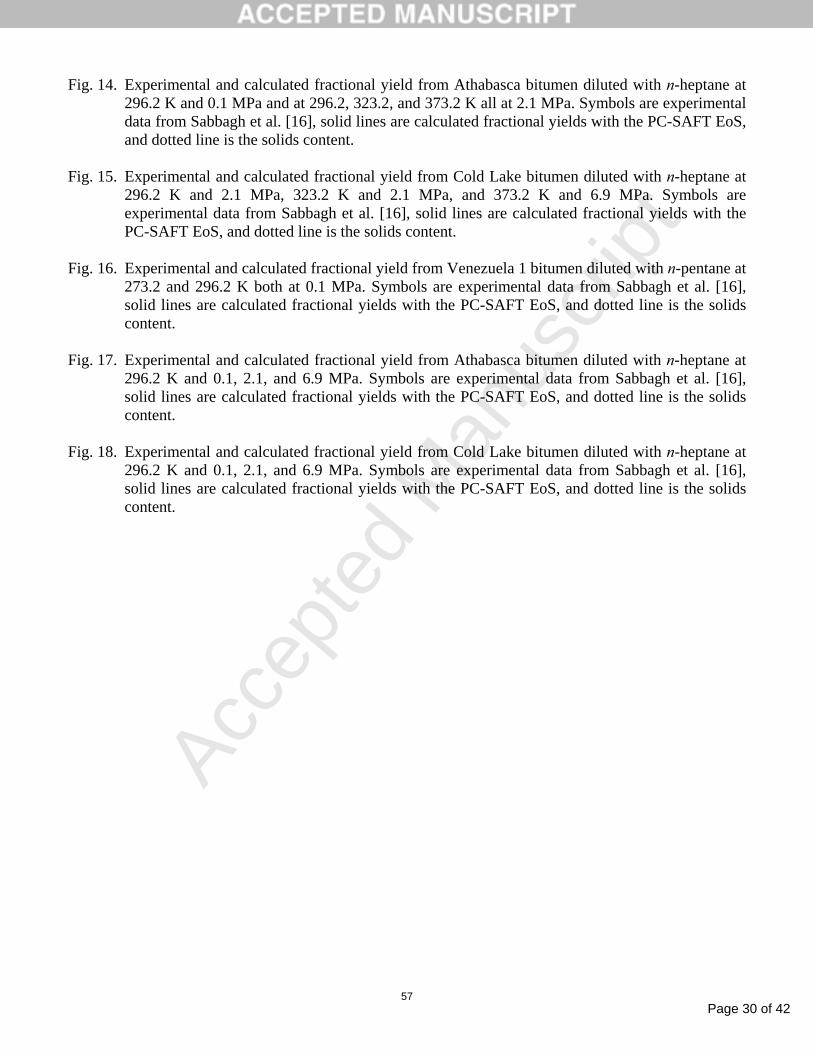
Fig. 14. Experimental and calculated fractional yield from Athabasca bitumen diluted with n-heptane at 296.2 K and 0.1 MPa and at 296.2, 323.2, and 373.2 K all at 2.1 MPa. Symbols are experimental data from Sabbagh et al. [16], solid lines are calculated fractional yields with the PC-SAFT EoS, and dotted line is the solids content.
Fig. 15. Experimental and calculated fractional yield from Cold Lake bitumen diluted with n-heptane at
296.2 K and 2.1 MPa, 323.2 K and 2.1 MPa, and 373.2 K and 6.9 MPa. Symbols are experimental data from Sabbagh et al. [16], solid lines are calculated fractional yields with the PC-SAFT EoS, and dotted line is the solids content.
Fig. 16. Experimental and calculated fractional yield from Venezuela 1 bitumen diluted with n-pentane at
273.2 and 296.2 K both at 0.1 MPa. Symbols are experimental data from Sabbagh et al. [16], solid lines are calculated fractional yields with the PC-SAFT EoS, and dotted line is the solids content.
Fig. 17. Experimental and calculated fractional yield from Athabasca bitumen diluted with n-heptane at
296.2 K and 0.1, 2.1, and 6.9 MPa. Symbols are experimental data from Sabbagh et al. [16], solid lines are calculated fractional yields with the PC-SAFT EoS, and dotted line is the solids content.
Fig. 18. Experimental and calculated fractional yield from Cold Lake bitumen diluted with n-heptane at
296.2 K and 0.1, 2.1, and 6.9 MPa. Symbols are experimental data from Sabbagh et al. [16], solid lines are calculated fractional yields with the PC-SAFT EoS, and dotted line is the solids content.

Page 31 of 42
Accep
ted
Man
uscr
ipt
58
kount = 0
kount = kount +1
YES
NO
values of Initiation K-
z,,,:Input PTnc
yxii
iic
yxzKn
θθβ ,,,,:Output,,:Input
routine Rice-Rachford Execute
),,(lnEvaluate),,(lnEvaluate
yx
PTfPTf
y
x
)(ln)(ln:errorvectorEvaluate
,, xixyiyi ffg θθ −−−=
phasesliquidTwoeconvergencNo
solutionTrivialnK
liquidphaseOne
liquidphaseOne
cn
ici
x
y
→→≥
→<
→>=
→>=
∑=
−
elsemaxitkount
10ln
2,0,1
1,0,0
1
42
θβ
θβ
1setorCalculate
=γγ
ik
ik
i gKKK-
γ−=+ )()1( lnln: valuesUpdate
ii yx ,,:Output
β
?maxitkount
or?101
82
≥
<∑=
−cn
iig
Figure 1. (Zúñiga-Hinojosa et al.)
Page 32 of 42
Accep
ted
Man
uscr
ipt
59
iter = iter+1iter = 0
iter > maxit ?
Stop
21
21
lli
iii
lli
ii
KzKY
KzX
ββ
ββ
+=
+=
NO
YES
NO
YES
z,,,:Input PTnc
∑=
<cn
iii zK
1?1
∑=
<cn
iii Kz
1?1/
1,0 21 == ll ββ
0,1 21 == ll ββ )(ln
)(ln
/
/
1
1
1
1
∑∑∑∑
=
=
=
=
−=
−=
=
=
c
c
c
c
n
i iy
n
i ix
n
j jii
n
j jii
Y
X
YYy
XXx
θ
θ
)]1/()1(,1min[1allFor
max ii
i
KzK
−−=<
β
)]1/()1(,0max[1allFor
min −−=>
iii
i
KzKK
β
?0)()( maxmin <⋅ ββ ff
?methodNewton or methodBisection
121 1, :Output methodBisection
lll βββ −=
NO
YES
12
maxmin1
1
2/)(:methodNewton
ll
l
ββ
βββ
−=
+= ∑= +
−=
cn
i lli
ii
KKzf
1 21
)1(ββ
∑= +
−−=
cn
i lli
ii
KKzf
12
21
2
)()1('
ββ
)(')(
1
1
l
l
ffββ
β −=Δ
1max1
1min1
1If
0If
ll
ll
βββββ
βββββ
−=Δ→>Δ+
+=Δ→<Δ+
?10)(
or?1010
10
−
−
≤
≤Δ
β
β
f
NO
YES
NO
12
11
1 ll
ll
ββ
βββ
−=
Δ+=
YES
Return
Figure 2. (Zúñiga-Hinojosa et al.)
Page 33 of 42
Accep
ted
Man
uscr
ipt
60
0
100
200
300
400
0 5000 10000 15000
m
Molar mass, g/mol
Saturates (Panuganti et al. [27, 36])
Asphaltenes (This work)
3.8
3.9
4.0
4.1
4.2
4.3
4.4
4.5
0 5000 10000 15000
σ, Å
Molar mass, g/mol
Saturates (Panuganti et al. [27, 36])
Asphaltenes (This work)
200
250
300
350
400
450
0 5000 10000 15000
ε/k, K
Molar mass, g/mol
Saturates (Panuganti et al. [27, 36])
Asphaltenes (This work)
Figure 3. (Zúñiga-Hinojosa et al.)

Page 34 of 42
Accep
ted
Man
uscr
ipt
61
0
5
10
15
20
25
30
100 300 500 700 900 1100
m
Molar mass, g/mol
Saturates (Panuganti et al.[27, 36])
Aromatics (Panuganti et al. [27, 36])
Resins (Panuganti et al. [27, 36])
Asphaltenes (This work)
Aromatics + Resins (f. aroma. = 0.01)
Saturates (Sabbagh et al. [16])
Aromatics (Sabbagh et al.[16])
Resins (Sabbagh et al. [16])
3.8
3.9
4.0
4.1
4.2
4.3
4.4
4.5
4.6
4.7
4.8
100 300 500 700 900 1100
σ, Å
Molar mass, g/mol
Saturates (Panuganti et al. [21]) Aromatics (Panuganti et al. [21])
Resins (Panuganti et al. [21]) Asphaltenes (This work)
Aromatics + Resins (f. arom. = 0.01) Saturates (Sabbagh et al [16])
Aromatics (Sabbagh et al. [16]) Resins (Sabbagh et al. [16])
200
250
300
350
400
450
500
550
600
100 300 500 700 900 1100
ε/k, K
Molar mass, g/mol
Saturates (Panuganti et al. [21]) Aromatics (Panuganti et al. [21])Resins (Panuganti et al. [21]) Asphaltenes (This work)Aromatics + Resins (f. arom. = 0.01) Saturates (Sabbagh et al. [16])Aromatics (Sabbagh et al. [16]) Resins (Sabbagh et al. [16])
Figure 4. (Zúñiga-Hinojosa et al.)
Page 35 of 42
Accep
ted
Man
uscr
ipt
62
kij = 0.0097wn-C5 - 0.0134
-0.009
-0.007
-0.005
-0.003
-0.001
0.5 0.6 0.7 0.8 0.9 1.0
Inte
ract
ion
Par
amet
er
n-C5 Mass Fraction
Adjusted interaction parameter
kij = 0.0021wn-C6 - 0.0078
-0.0068
-0.0066
-0.0064
-0.0062
-0.0060
-0.0058
0.5 0.6 0.7 0.8 0.9 1
Inte
ract
ion
Para
met
er
n-C6 Mass Fraction
Adjusted interaction parameter
kij = 0.0034wn-C7 - 0.0076
-0.0060
-0.0056
-0.0052
-0.0048
-0.0044
-0.0040
0.5 0.6 0.7 0.8 0.9 1.0
Inte
ract
ion
Par
amet
er
n-C7 Mass Fraction
Adjusted interaction parameter
Figure 5. (Zúñiga-Hinojosa et al.)

Page 36 of 42
Accep
ted
Man
uscr
ipt
63
kij = 0.0068wn-C7 - 0.0105
-0.0065
-0.0060
-0.0055
-0.0050
-0.0045
-0.0040
0.6 0.7 0.8 0.9 1.0
Inte
ract
ion
Para
met
er
n-C7 Mass Fraction
Adjusted interaction parameter at 296.2 K and 2.1 MPa
kij = -0.0183wn-C7 + 0.0141
-0.004
-0.003
-0.002
-0.001
0.000
0.001
0.002
0.003
0.6 0.7 0.8 0.9 1.0
Inte
ract
ion
Par
amet
er
n-C7 Mass Fraction
Adjusted interaction parameter at 373.2 K and 2.1 MPa
kij = 0.0103wn-C7 - 0.0152
-0.010
-0.009
-0.008
-0.007
-0.006
-0.005
0.5 0.6 0.7 0.8 0.9 1.0
Inte
ract
ion
Par
amet
er
n-C7 Mass Fraction
Adjusted interaction parameter at 273.2 K and 0.1 MPa
kij = -0.0031wn-C7 - 0.0001
-0.0035
-0.0030
-0.0025
-0.0020
-0.0015
-0.0010
0.5 0.6 0.7 0.8 0.9 1.0
Inte
ract
ion
Para
met
er
n-C7 Mass Fraction
Adjusted interaction parameter at 323.2 K and 2.1 MPa
Figure 6. (Zúñiga-Hinojosa et al.)
Page 37 of 42
Accep
ted
Man
uscr
ipt
64
0.00
0.02
0.04
0.06
0.08
0.10
0.12
0.14
0.16
0.2 0.4 0.6 0.8 1
Frac
tiona
l Yie
ld
n-Alkane Mass Fraction
n-Pentane
n-Hexane
n-Heptane
Figure 7. (Zúñiga-Hinojosa et al.)
0.00
0.02
0.04
0.06
0.08
0.10
0.12
0.14
0.16
0.18
0.2 0.4 0.6 0.8 1
Frac
tiona
l Yie
ld
n-Alkane Mass Fraction
n-Pentane
n-Hexane
n-Heptane
Figure 8. (Zúñiga-Hinojosa et al.)
Page 38 of 42
Accep
ted
Man
uscr
ipt
65
0.00
0.02
0.04
0.06
0.08
0.10
0.12
0.14
0.16
0.18
0.2 0.4 0.6 0.8 1
Frac
tiona
l Yie
ld
n-Alkane Mass Fraction
n-Pentane
n-Hexane
n-Heptane
Figure 9. (Zúñiga-Hinojosa et al.)
0.00
0.02
0.04
0.06
0.08
0.10
0.12
0.14
0.16
0.18
0.2 0.4 0.6 0.8 1
Frac
tiona
l Yie
ld
n-Alkane Mass Fraction
n-Pentane
n-Heptane
Figure 10. (Zúñiga-Hinojosa et al.)
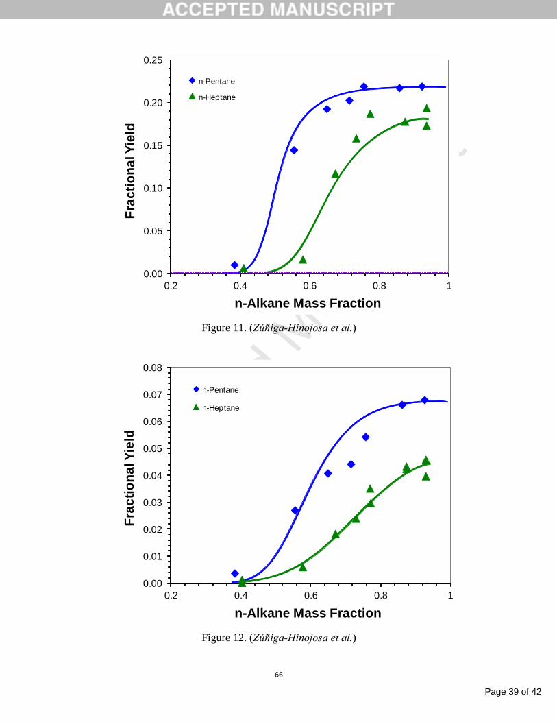
Page 39 of 42
Accep
ted
Man
uscr
ipt
66
0.00
0.05
0.10
0.15
0.20
0.25
0.2 0.4 0.6 0.8 1
Frac
tiona
l Yie
ld
n-Alkane Mass Fraction
n-Pentane
n-Heptane
Figure 11. (Zúñiga-Hinojosa et al.)
0.00
0.01
0.02
0.03
0.04
0.05
0.06
0.07
0.08
0.2 0.4 0.6 0.8 1
Frac
tiona
l Yie
ld
n-Alkane Mass Fraction
n-Pentane
n-Heptane
Figure 12. (Zúñiga-Hinojosa et al.)
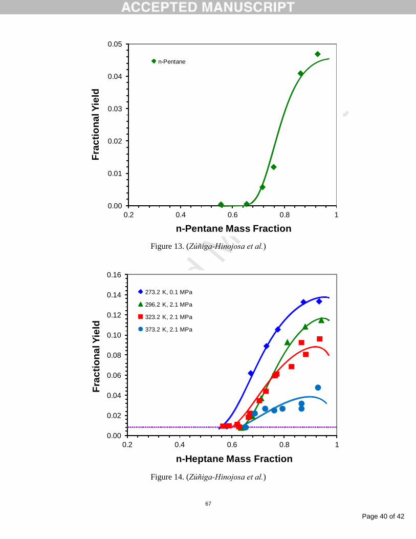
Page 40 of 42
Accep
ted
Man
uscr
ipt
67
0.00
0.01
0.02
0.03
0.04
0.05
0.2 0.4 0.6 0.8 1
Frac
tiona
l Yie
ld
n-Pentane Mass Fraction
n-Pentane
Figure 13. (Zúñiga-Hinojosa et al.)
0.00
0.02
0.04
0.06
0.08
0.10
0.12
0.14
0.16
0.2 0.4 0.6 0.8 1
Frac
tiona
l Yie
ld
n-Heptane Mass Fraction
273.2 K, 0.1 MPa
296.2 K, 2.1 MPa
323.2 K, 2.1 MPa
373.2 K, 2.1 MPa
Figure 14. (Zúñiga-Hinojosa et al.)
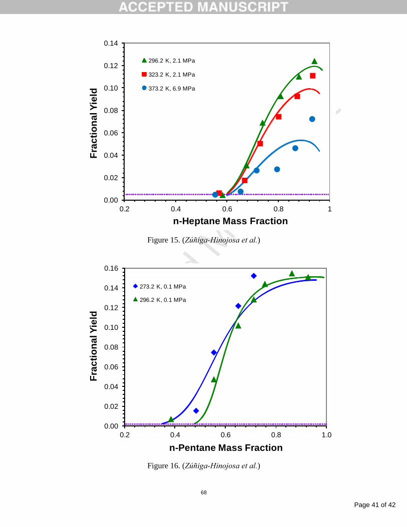
Page 41 of 42
Accep
ted
Man
uscr
ipt
68
0.00
0.02
0.04
0.06
0.08
0.10
0.12
0.14
0.2 0.4 0.6 0.8 1
Frac
tiona
l Yie
ld
n-Heptane Mass Fraction
296.2 K, 2.1 MPa
323.2 K, 2.1 MPa
373.2 K, 6.9 MPa
Figure 15. (Zúñiga-Hinojosa et al.)
0.00
0.02
0.04
0.06
0.08
0.10
0.12
0.14
0.16
0.2 0.4 0.6 0.8 1.0
Frac
tiona
l Yie
ld
n-Pentane Mass Fraction
273.2 K, 0.1 MPa
296.2 K, 0.1 MPa
Figure 16. (Zúñiga-Hinojosa et al.)

Page 42 of 42
Accep
ted
Man
uscr
ipt
69
0.00
0.02
0.04
0.06
0.08
0.10
0.12
0.14
0.2 0.4 0.6 0.8 1
Frac
tiona
l Yie
ld
n-Heptane Mass Fraction
296.2 K, 0.1 MPa
296.2 K, 2.1 MPa
296.2 K, 6.9 MPa
Figure 17. (Zúñiga-Hinojosa et al.)
0.00
0.02
0.04
0.06
0.08
0.10
0.12
0.14
0.2 0.4 0.6 0.8 1
Frac
tiona
l Yie
ld
n-Heptane Mass Fraction
296.2 K, 0.1 MPa
296.2 K, 2.1 MPa
296.2 K, 6.9 MPa
Figure 18. (Zúñiga-Hinojosa et al.)