Modeling of electric field distribution in tissues during ...lbk.fe.uni-lj.si/pdfs/be2013sc.pdf · Modeling of electric field distribution in tissues during electroporation Selma

Corovic et al. BioMedical Engineering OnLine 2013, 12:16http://www.biomedical-engineering-online.com/content/12/1/16

RESEARCH Open Access

Modeling of electric field distribution in tissuesduring electroporationSelma Corovic1, Igor Lackovic2, Primoz Sustaric3, Tomaz Sustar3, Tomaz Rodic3 and Damijan Miklavcic1*

* Correspondence: [email protected] of Ljubljana, Faculty ofElectrical Engineering, Trzaska cesta25, SI-1000 Ljubljana, SloveniaFull list of author information isavailable at the end of the article

Abstract

Background: Electroporation based therapies and treatments (e.g. electrochemotherapy,gene electrotransfer for gene therapy and DNA vaccination, tissue ablation withirreversible electroporation and transdermal drug delivery) require a precise prediction ofthe therapy or treatment outcome by a personalized treatment planning procedure.Numerical modeling of local electric field distribution within electroporated tissues hasbecome an important tool in treatment planning procedure in both clinical andexperimental settings. Recent studies have reported that the uncertainties in electricalproperties (i.e. electric conductivity of the treated tissues and the rate of increase inelectric conductivity due to electroporation) predefined in numerical models have largeeffect on electroporation based therapy and treatment effectiveness. The aim of ourstudy was to investigate whether the increase in electric conductivity of tissues needs tobe taken into account when modeling tissue response to the electroporation pulses andhow it affects the local electric distribution within electroporated tissues.

Methods: We built 3D numerical models for single tissue (one type of tissue, e.g. liver)and composite tissue (several types of tissues, e.g. subcutaneous tumor). Our computersimulations were performed by using three different modeling approaches that arebased on finite element method: inverse analysis, nonlinear parametric and sequentialanalysis. We compared linear (i.e. tissue conductivity is constant) model and non-linear (i.e. tissue conductivity is electric field dependent) model. By calculatinggoodness of fit measure we compared the results of our numerical simulations tothe results of in vivo measurements.

Results: The results of our study show that the nonlinear models (i.e. tissueconductivity is electric field dependent: σ(E)) fit experimental data better thanlinear models (i.e. tissue conductivity is constant). This was found for both singletissue and composite tissue. Our results of electric field distribution modeling inlinear model of composite tissue (i.e. in the subcutaneous tumor model that donot take into account the relationship σ(E)) showed that a very high electric field(above irreversible threshold value) was concentrated only in the stratum corneumwhile the target tumor tissue was not successfully treated. Furthermore, thecalculated volume of the target tumor tissue exposed to the electric field abovereversible threshold in the subcutaneous model was zero assuming constantconductivities of each tissue.Our results also show that the inverse analysis allows for identification of bothbaseline tissue conductivity (i.e. conductivity of non-electroporated tissue) andtissue conductivity vs. electric field (σ(E)) of electroporated tissue.(Continued on next page)

© 2013 Corovic et al.; licensee BioMed Central Ltd. This is an Open Access article distributed under the terms of the CreativeCommons Attribution License (http://creativecommons.org/licenses/by/2.0), which permits unrestricted use, distribution, andreproduction in any medium, provided the original work is properly cited.

mailto:[email protected]

mailto:[email protected]

http://creativecommons.org/licenses/by/2.0

Corovic et al. BioMedical Engineering OnLine 2013, 12:16 Page 2 of 27http://www.biomedical-engineering-online.com/content/12/1/16

(Continued from previous page)

Conclusion: Our results of modeling of electric field distribution in tissues duringelectroporation show that the changes in electrical conductivity due to electroporationneed to be taken into account when an electroporation based treatment is planned orinvestigated. We concluded that the model of electric field distribution that takes intoaccount the increase in electric conductivity due to electroporation yields more preciseprediction of successfully electroporated target tissue volume. The findings of our studycan significantly contribute to the current development of individualized patient-specificelectroporation based treatment planning.

Keywords: Electroporation, Numerical modeling, Inverse analysis, Electric fielddistribution, Tissue conductivity, Liver electroporation, Tumor electroporation

BackgroundElectroporation is an increase of cell membrane permeability to molecules that other-

wise lack efficient transmembrane transport mechanisms. Due to membrane electro-

poration cell membrane conductivity is also increased. Electroporation can be achieved

if cells are exposed to a sufficiently high electric field induced by application of high

voltage pulses (i.e. electroporation pulses) [1-3]. The efficiency of electroporation

strongly depends on pulse parameters such as pulse amplitude, pulse duration, number

of pulses and repetition frequency [4]. In order to successfully electropermeabilize a cell

membrane the induced transmembrane voltage needs to exceed a given value that de-

pends on cell or tissue type (e.g. cell geometry, cell density, cell’s shape and orientation

with respect to the electric field) [5-9]. It has been demonstrated that all types of cells

(e.g. human, animal, plant and microorganisms) can be effectively electroporated, pro-

vided that appropriate electroporation parameters are selected for each of the cell or

tissue type [10]. One of the key parameters for effective cell and tissue electroporation

is however adequate electric field distribution within the treated sample [11]. The local

electric field induces the transmembrane voltage on the cell [12,13], which is in turn

correlated with transmembrane flux [3]. A cell or tissue is reversibly electroporated

when the local electric field exceeds a reversible threshold value (Erev) [14-16]. If the

local electric field however exceeds an irreversible threshold (Eirrev) value the mem-

branes of the exposed cells are disrupted to such an extent that cells fail to recover and

they die (i.e. irreversible electroporation) [17-19].

Increase in cell membrane permeability allows for both administration of different

molecules into electroporated cells (such as therapeutic drugs or molecular probes,

which otherwise can not enter the cytosol) and for extraction of different cell compo-

nents out from the cells [20,21]. Since, electroporation has been demonstrated to be a

versatile method for both in vitro and in vivo settings it has been successfully applied

to various domains such as medicine (e.g. human and veterinary oncology) [22-27],

food processing [28] and microbial inactivation in water treatment [29].

Medical electroporation based therapies and treatments such as electrochemotherapy

in local tumor control [27,30], tissue ablation method by means of irreversible electro-

poration [31,32] and gene therapy and DNA based vaccination by means of gene

electrotransfer [33,34] are paving their way into clinical practice. In particular,

electrochemotherapy has been demonstrated as an efficient tumor treatment as 85%

objective response was obtained in treating skin metastasis of various cancers. In 2006


electrochemotherapy standard operating procedures (SOP) have been defined for the

treatment of easily accessible cutaneous and subcutaneous tumor nodules of different

histologies [35]. The SOP for electrochemotherapy were defined based on external pa-

rameters such as amplitude of applied voltage and distance between electrodes based

on preclinical results and the results of numerical calculations in 3D models (1300 V/

cm and 1000 V/cm for plate and needle electrodes respectively) [13,15]. The efficacy of

SOP for easily accessible cutaneous tumors and subcutaneous tumor (depth: less than

2 cm) nodules were later confirmed by numerous clinical studies [30,36-38]. The

in vivo studies that were based also on numerical simulations further demonstrated that

the protocols of cutaneous tumors can be refined and that the electrochemotherapy

can be successfully applied to deep-seated tumors based on analysis of local electric

field distribution within the tumors [39,40]. In our previous study [41] we demon-

strated that better electrochemotherapy outcome of cutaneous tumors can be obtained

with increase of contact surface between plate electrodes and treated tissue. Similarly,

Ivorra and colleagues [42] proposed the use of conductive gels in order to ‘homogenize’

the electric field within the treated tissue of easily accessible cutaneous tumors. How-

ever, for deep-seated tumors and tumors in internal organs, such as for example liver,

brain or muscle tissue that are surrounded by other tissues having different electric

properties an individualized patient-specific treatment planning is required as the het-

erogeneity of local electric field distribution within all exposed tissues can not be

neglected [43,44]. Namely, several preclinical and clinical studies have shown that

deep-seated tumors located in internal organs (breast cancer [27,37], bone metastasis

[45], brain [46], liver metastases [40], melanoma metastasis in the muscle [39]) are also

treatable. The outcome of the treatment however greatly depends on positioning of the

electrodes, on applying of adequate pulses, electrode geometry and electrical properties

of the treated tissues. These findings were either predicted or confirmed with numerical

simulations, which resulted in development of computer-based treatment planning

of both reversible electroporation based therapies (such as electrochemotherapy

[43,44,47-49] and gene therapy and vaccination [50]) and irreversible electroporation

based therapies [47,51-53]. Development of treatment planning of electroporation

based therapies is currently focused on analysis of the shape and position of electrodes

used and applied voltage to the electrodes [40,44,54,55]. Numerous studies demon-

strated that the conductivity is increased due to membrane electroporation [2,56,57]

and that in calculating the local electric field distribution within treated tissue one

needs to account for these tissue conductivity increases [9,16,47,58,59]. In preclinical

and clinical studies authors however often consider the treated tissues as being linear

electric conductors (i.e. with constant tissue conductivities).

The aim of our study was to investigate whether the increase in electric conductivity

of tissues needs to be taken into account when modeling tissue response to the electro-

poration pulses and how it affects the local electric field distribution within

electroporated tissues. We also attempted to identify the nature of functional dependency

of tissue conductivity on electric field. We therefore compared linear (i.e. tissue conductiv-

ity is constant) and non-linear (i.e. tissue conductivity is electric field dependent) model to

the experimental data in vivo [56]. The study was performed for both single tissue (one

type of tissue, e.g. liver) and composite tissue (several types of tissues, e.g. subcutaneous

tumor). Our computer simulations were performed by using three different modeling


approaches: 1. inverse analysis (IA) [60,61], 2. nonlinear parametric analysis (NPA) [62]

and 3. sequential analysis (SA) [58]. The algorithm for IA modelling approach has

been previously developed by [60,61] to model different physical phenomena in wide

range of research and industry including biomechanics, pharmaceutical industry and

space [63]. In this paper we introduced and successfully applied the IA approach for

the first time in the field of modelling of biophysical processes that occur during tis-

sue electroporation.

The results of all three modeling approaches are then compared to the results of

our previous experimental measurements in vivo [56]. The results of our present

study show that the nonlinear models fit experimental data better than linear

models. We also demonstrate that tissue conductivity as a function of local electric

field need to be taken into account when an electroporation based therapy or treat-

ment is planned.

Materials and methodsIn order to investigate the change of electric properties of tissues on the electric field

distribution during electroporation we built 3D numerical models of single tissue and

composite tissue.

Modeling of electric field distribution in a single tissue during electroporation was

carried out in liver tissue. We analyzed experimental data for plate and needle elec-

trodes. Original experiments with plate electrodes were performed in rat liver, while

the experiments with needle electrodes were performed in rabbit liver [56].

Modeling of electric field distribution in composite tissue (i.e. tissue composed of dif-

ferent types of tissues) was carried out in cutaneous tumor tissue. In vivo experiments

were performed in mice with plate electrodes for two different types of cutaneous tu-

mors: B16 and LPB sarcoma within the study by [56].

The high voltage pulses in all in vivo experiments were applied to the electrodes

according to the electroporation protocol of eight 100 μs long pulses delivered to the

tissues with 1 Hz repetition frequency. Within the experiments [56] the real time tissue

electroporation control was performed by monitoring and measuring the electric

current during the delivery of electric pulses. In order to evaluate the tissue electropor-

ation efficiency during the pulse delivery the 51CrEDTA indicator was used for all tis-

sues. The system for the real time tissue electroporation control and 51CrEDTA uptake

measurements were described in our previous work [56]. The electric current measured

during the in vivo experiments provides the information about the bulk tissue conduct-

ivity changes during the pulse delivery.

In order to compare and evaluate the results of our numerical models to the experi-

mental data we calculated the goodness-of-fit measure R2 between numerically calcu-

lated and in vivo measured electric current I [A] at the end of the last delivered pulse

(i.e. the 8-th pulse) to the tissue.

Numerical modeling

Electric field distribution in the models of tissue exposed to electroporation pulses U

[V] can be determined by solving the equation (Eq. 1) for scalar electric potential.

Namely, if we neglect the capacitive transient and time course of conductivity increase


during the pulse, we may assume that the current density in tissue is divergence free

and electric potential satisfies:

� ∇⋅ σ⋅∇φð Þ ¼ 0 ð1Þ

where σ and φ represent tissue conductivity [S/m] and electric potential [V], respectively.

Applied voltage (model input) was modeled as Dirichlet’s boundary condition on the

contact surface between electrode and tissue geometry. For the model input values we

used the amplitudes of the electroporation pulses applied in vivo [56]. In order to

mathematically separate the conductive segment from its surroundings we applied

Neuman’s boundary condition (Jn = 0, where Jn is the normal electric current density

[A/m2]) on all outer boundaries of our models.

As long as the applied voltage U [V] is low enough the tissue conductivity σ [S/m]

can be treated as a constant (i.e. σ = const. in Eq. 1), the problem is therefore described

by the Laplace’s equation which is a linear partial differential equation that can be easily

solved numerically. In this case the tissues can be modeled as a linear conductor with

linear current–voltage I(U) relationships due to the constant tissue conductivities since

the amplitude of the applied electroporation pulses is too low to produce an E above

the reversible electroporation threshold (E < Erev).

However, to account for experimentally observed tissue conductivity increase due to elec-

troporation, Eq. 1 becomes nonlinear partial equation as σ is no longer constant. If the local

electric field in the tissues exceeds the Erev value, electric properties of treated tissue change

(i.e. tissue conductivity increases due to the electroporation process). In this case the σ in

Eq.1 depends on the electric field intensity E: σ = σ(E). Namely, during the application of

electroporation pulses, tissue conductivity increases according to the functional dependency

of the tissue conductivity on the local electric field distribution σ(E), which in our study de-

scribes the dynamics of the electroporation process. This subsequently results in nonlinear

electric current voltage relationship I(U) (i.e. numerical model of tissue is non-linear).

Measurement of electric current I [A] during delivery of eight rectangular electropor-

ation pulses of 100 μs duration and 1 Hz repetition showed that after rapid capacitive

transient (which is due to tissue capacitance) the current increased towards the end of

the pulse [56,52]. The rate of increase of electric current I [A] depends on the applied

voltage U [V], which provides information about the changes in electric properties of

the treated tissue (i.e. changes in electric conductivity of the tissue σ [S/m]). The rates

of increase of I and σ thus allow us to identify the degree of tissue electroporation.

Numerical calculations of Eq.1 and tissue electroporation dynamics σ(E) in our study

were performed with three different approaches that were based on finite element

method: Inverse analysis (IA), nonlinear parametric analysis (NPA) and sequential ana-

lysis (SA). The software for IA was previously developed by Center for Computational

Continuum Mechanics (Ljubljana, Slovenia) [61], while for the NPA and the SA we

used Comsol Multiphysics software (version 3.5a, COMSOL, Sweden).

The three abovementioned modeling approaches are described here below:

Inverse analysis (IA)

The IA is based on standard Newton–Raphson method, which is widely used for calcu-

lating nonlinear problems based on finite element method. The tissue electroporation

dynamics i.e. the dependence of the electrical conductivity with respect to electrical


field strength σ(E) is described by linear and exponential relationships. Unknown parame-

ters of these relationships are calculated by IA [60]. The IA is performed by using a sym-

bolic system AceGen (Multi-language, Multi-environment Numerical Code Generation)

[64] with AceFeM environment (The Mathematica Finite Element Environment) [65] for

development of finite element equations and generation of corresponding finite element

user subroutines. This enables symbolic formulation of the problem at a high abstract

level. The derivation presented here follows a general approach to the automation of pri-

mal and sensitivity analysis of transient problems introduced by [66]. Below is a brief de-

scription of the formulation.

The response of the steady-state non-linear problem is defined by the global residual

vector R and the vector of unknown variables of the problem φ (Eq. 2):

R φð Þ ¼ �Xe

Re φð Þ ¼ 0 ð2Þ

where Re represents the contribution of the e-th element to the global residual and e is

the element number. The operator *Σ is chosen here instead of the ordinary Σ symbol in

order to denote that an assembly process takes place in which all element contributions

have not only to be added up but also the kinematical compatibility between the elements

has to be fulfilled [60]. The residual vector R is a part of standard notation used in finite

element analysis. The finite element problems are represented by a set of equations in the

residual form, which are solved iteratively using the Newton–Raphson method. The sys-

tem given by the Eq. 2 can therefore be solved by the Newton–Raphson method, in which

the following iteration is performed according to Eq. 3 and Eq. 4:

dRdφ

φ ið Þ� �

Δφ ¼ �R φ ið Þ� �

ð3Þ

φ iþ1ð Þ ¼ φ ið Þ þ Δφ ð4Þ

The terms R(φ(i)) and dR φ ið Þ� �are referred to as the residual (or load) vector and the
dφ
tangent operator (or tangential stiffness matrix), respectively. The independent solution

vector φ(i) is updated after the linear system given by the Eq. 3 has been solved for the

unknown increment Δφ. The upper index (i) refers to the quantities at the i-th iteration

step of the outer loop.

The distribution of static electric field is determined by solving the Eq. 1. By using in-

tegral form and Galerkin approximation one can obtainZV

∇δφ:σ:∇φdV �ZS

J :nδφdS ¼ 0 ð5Þ

where φ is the electric potential,V is volume, S is surface and J is current density.

Discretization of Eq. 5 by φ =Ne. φe and δφ =Ne. δφe =Ne leads to the Eq. 6:

Re φð Þ ¼ZVe

∇Ne:σ: ∇Neð ÞT dV

264

375:φe ð6Þ

where φ is the electric potential, φe are the electrical potentials in the element nodes, δφis the test function, Ne are the nodal shape functions and σ is the electrical conductivity.


We considered linear (Eq. 7) and exponential (Eq. 8) dependences of tissue conduct-

ivity σ with respect to electric field strength E as follows:

σ Eð Þ ¼ σ0 þ kσ Eð Þ I ð7Þσ Eð Þ ¼ σ0 þ c1 ec2 E � 1

� �� I ð8Þ

where electric field strength E is defined as:

E ¼ �∇φE ¼ ffiffiffiffiffiffiffiffi

E:Ep ð9Þ

and I is the identity matrix. The constant in Eq. 7 and Eq. 8 stands for the baseline tis-

sue conductivity of non-electroporated tissue (i.e. σ0 = σ(0)), while the constants kσ, c1and c2 stand for the parameters of linear (Eq. 7) and exponential (Eq. 8) functions de-

scribing electroporated tissue (i.e.σ(E)).

Unknown coefficients σ0, kσ, c1 and c2 were determined with IA [60] by minimizing

the objective function f of the following form:

f σ0; kσ ; c1; c2ð Þ ¼Xj

IFEM � Imeasured

U

� �2

jð Þð10Þ

Determination of unknown coefficients σ0, kσ, c1 and c2 allowed us to detect the

properties of the treated tissue for both situations σ = const. (i.e. σ0 = σ(0)) and σ(E)).

By using the Newton's method in the Mathematica (version 8.0) programming envir-

onment the minimization problem is defined as:

g x ¼ σ0; kσ ; c1; c2f gð Þ ¼

∂f σ0; kσ ; c1; c2ð Þ∂σ0

¼Xj

2IFEM � Imeasured

U2

∂IFEM∂σ0

� �jð Þ;

∂f σ0; kσ ; c1; c2ð Þ∂kσ

¼Xj

2IFEM � Imeasured

U2

∂IFEM∂kσ

� �jð Þ

∂f σ0; kσ ; c1; c2ð Þ∂c1

¼Xj

2IFEM � Imeasured

U2

∂IFEM∂c1

� �jð Þ

∂f σ0; kσ ; c1; c2ð Þ∂c2

¼Xj

2IFEM � Imeasured

U2

∂IFEM∂c2

� �jð Þ

8>>>>>>>>>>>>><>>>>>>>>>>>>>:

9>>>>>>>>>>>>>=>>>>>>>>>>>>>;

¼ 0

ð11Þ

where U is the voltage between the electrodes, IFEM is the calculated current and

Imeasured the measured current in the j-th measurement. The derivatives ∂IFEM∂σ0

, ∂IFEM∂kσ

, ∂IFEM∂c1

and ∂IFEM∂c2

were calculated within the finite element method analysis.

Nonlinear parametric analysis (NPA)

The NPA has been developed in our previous study [62]. In the present study we

used NPA to solve the equation Eq. 1 for both conditions σ = const. (for E < Erev) and

σ = σ(E) (for E ≥ Erev) by using Comsol Multiphysics’ stationary nonlinear solver.

Namely, we treat the problem as stationary since we analyzed the tissue behavior by

calculating the σ(E) dependency at the end of the applied pulse U [V]. The parame-

ters defined by NPA are the values of the applied voltages U (i.e. model inputs). The

electric current I [A] is calculated as a model output providing the value of I [A] at

the end of pulse. The Comsol Multiphysics’ nonlinear solver uses an affine invariant


form of damped Newton method. The user must supply an initial guess for the

dependent variable U (i.e. U0). Starting with the initial guess, the software forms the

linearized model using U0 as the linearization point i.e. the discrete form of the

equations as f(U) = 0, where f(U) is the residual vector and U is the solution vector.

The iterative Newton method can be applied in the usual way, expanding the re-

sidual vector in a Taylor series, neglecting all but the first order term. The software

solves the discretized form of the linearized model f ’(U0)δU = −f(U0) for the Newton

step δU by using the selected linear system solver (the f ’(U0) is the Jacobian matrix).

It then computes the new iterate U1 = U0 + λδU, where λ is the damping factor. The

modified Newton correction then estimates the error Eerror for the new iterate U1 by

solving f ’(U0)Eerror = −f(U1). If the relative error corresponding to E is larger than the

relative error in the previous iteration, the code reduces the damping factor λ and

recomputes U1. This algorithm repeats the damping-factor reduction until the relative

error is less than in the previous iteration or until the damping factor underflows the

minimum damping factor. When it has taken a successful step U1, the algorithm proceeds

with the next Newton iteration. A value of λ = 1 results in Newton’s method, which con-

verges quadratically if the initial guess U0 is sufficiently close to the solution. Comsol

Multiphysics will reduce the damping factor and re-compute U1 if the relative error is lar-

ger than the previous value. The purpose of this damping factor is to make the process

converge for a broader range of initial values (initial guesses U0).

It is necessary to increase the voltage U from 0 V in small steps and use the solution

from a previous step as the initial condition for the next step. This is taken care of

automatically by the parametric solver. The parametric solver consists of a loop around

the stationary solver. If the nonlinear solver does not converge it tries a smaller param-

eter step; if it does converge it determines the size of the next parameter step based on

the speed of the convergence of the Newton iteration.

Sequential analysis (SA)

The SA in our study was based on the sequential permeabilization model proposed by

[58], where changes in tissue conductivity were used as an indicator of tissue

permeabilization. Namely, the dynamics of electroporation was modeled as a discrete

process with the sequence of static finite element models. Each of the finite element

models described the process in one discrete interval (each of the discrete intervals re-

lates to a real, discrete, but undetermined time interval). In each static finite element

model in sequence, the tissue conductivity was determined based on the electric field

distribution from the previous model in the sequence according to the Eq. 12:

σ kð Þ ¼ f E k � 1ð Þð Þ ð12Þ

where k stands for the number of static finite element models in sequence.

Model input is the applied voltage pulse, and model outputs are the electric field dis-

tribution E and total electric current I in each specific sequence k. The increase in elec-

trical current I from I0 to Ik simulates the tissue response during the delivery of the

electroporation pulses U in each discrete interval k (static finite element model in se-

quence) to the tissue electroporation (i.e. due to the functional dependency of σ on the

electric field distribution E). If the electroporation does not occur, σ remains constant,

thus I = I0. More detailed description of SA is given in [16,58,59].


The numerical calculations obtained with NPA and SA by using COMSOL Multiphysics

3.5a software package were performed in the 3D Conductive Media DC application mode

on a computer running Windows XP (64 bit) with a 3.00 GHz Intel Pentium D processor

and 2 GB of RAM.

For the numerical calculations with IA we used AceGen (version AceFEM 3.101) sys-

tem [61,64,65]. The calculations were performed on a computer running Windows XP

(64 bit) with 2.67 GHz Intel Core i7 CPU and 6 GB of RAM.

Results of numerically calculated model outputs (such as total current and local elec-

tric field distribution) with all three approaches were controlled for numerical errors by

increasing the mesh density until the output results changed by less that 0.5%. The

mesh of the resulting finite element models of liver tissue electroporated with plate and

needle electrodes were composed of approximately 30 000 and 25 400 elements, re-

spectively. Number of generated finite elements of the tumor mesh model was 30 268.

Model geometry and electric properties of a single tissue

The 3D geometry of the numerical model and its 2D cross-sectional view in XY plane

of a single tissue (i.e. liver tissue) is given in Figure 1. The model of liver tissue

electroporated with plate electrodes is given in Figure 1A, while the model of liver tis-

sue electroporated with a pair of needle electrodes is given in Figure 1B.

By using the IA numerical simulations we identified both baseline electric conductiv-

ity of tissue σ0 (for the condition σ(0)) and linear and exponential σ(E) (Eqs. 7 and 8)

that fitted best the experimental data in vivo [56]. The determined σ0 and σ(E) for plate

and needle electrodes were then compared to the data from the literature.

Figure 1 Geometry of numerical models of liver tissue. A. treated with plate electrodes and B. treatedwith needle electrodes. The parameter σL stands for the conductivity σ [S/m] of liver tissue.


Since the NPA and SA required the baseline tissue conductivity σ0, the conductivity

increase factor due to electroporation, the reversible and ireversible threshold values

(Erev and Eirrev) to be predefined, in our models we selected the data from [58,62,67,68].

The functional dependencies σ(E) predefined in the models were sigmoid-like func-

tion implemented as smoothed Heaviside's step function [62] with continuous sec-

ond derivative and sigmoid function σ(E) that was implemented by Sel and

colleagues [58].

Model geometry and electric properties of composite tissue

The geometry of composite tissue i.e. subcutaneous tumor is shown in Figure 2A. The

distance between two plate electrodes used in experiments was d = 5.2 mm. The tumor

geometry was created so as to match as accurate as possible the electrode placement

and the geometry of the tissue treated within the in vivo experiments. The electrodes

in Figure 2A only sketch the site of electrodes’ position in the experiments and do not

take part of the numerical model. The body of the electrodes was not modeled in our

numerical model in order to reduce the computation time of numerical simulations.

The electrodes were modeled rather as boundary conditions defined on the electrode-

tissue contact surfaces (Figure 2B).

The numerical model of the tumor was built as a heterogeneous 3D model composed

of four types of tissues with different electric properties (i.e. electric conductivities).

The skin in our subcutaneous tumor model was modeled as two-layer tissue: the first

layer comprised the electric properties of stratum corneum and epidermis (σSE), while

the second layer comprised dermis and fat tissue (σDF). The underlying muscle tissue

was modeled as anisotropic tissue with σM⊥ (Y and Z direction -Figure 2) and σM|| (X

direction - Figure 2) in perpendicular and parallel direction of E with respect to the

muscle fibers. The baseline conductivities of the modeled tissues (i.e. the initial σ of

non-electroporated tissues for E < Erev), the conductivity increase factor due to tissue

electroporation and the threshold values Erev and Eirrev for each of the tissues were se-

lected based on data we published previously [9,16,59,69]and based on the comparison

Figure 2 Geometry of numerical model of subcutaneous tumor. A. The geometry dimensions andcomposition of cutaneous tumor model. (The electrodes in this figure only sketch the site of electrodes’position in the experiments and do not take part of the numerical model) and B. 3D geometry of tumormodel with the contact surface between tissue and electrodes. The distance between plate electrodeswas d = 5.2 mm.


of I [A] calculated in our models to the in vivo measurements. Our numerical and ex-

perimental analysis was performed for two different types of cutaneous tumors: B16

melanoma and LPB sarcoma.

The relationship of electric conductivity with respect to the local electric field σ(E)

for all modeled tissues was considered to be smoothed Heaviside step function taking

into account the electric conductivities and the threshold values data listed in Table 1.

For the numerical calculations we used NPA. We examined the electric current and

local electric field distribution within the model of subcutaneous tumor for three differ-

ent electric properties of target tumor tissue σT1, and σT2 and σT3.

Statistical analysis

To compare the outputs of our models to the experimentally measured data we calcu-

lated coefficient of determination R2, which represents a statistical measure of how well

the model data approximates the real data points (i.e. the measure of the goodness-of

-fit between the modeled and measured data). The R2 = 1 means that the model data

perfectly fit the real data points. If the R2 has a value closer to the 0 or a negative value

the model data do not fit the real data points.

The coefficient of determination is given by the Eq.13.

R2 ¼ 1� SSerrSStot

ð13Þ

where SSerr and SStot are residual sum of squares and the total sum of squares,

respectively.

The "variability" of the data set is measured through the sums of squares SSerr and

SStot.

The residual sum of squares SSerr is defined by the Eq. 14:

SSerr ¼Xi

yi � fið Þ2 ð14Þ

where yi data stand for the measured values of electric current at the end of the pulse,

each of which has an associated modeled value fi.

Table 1 The defined parameters of tissues composing the subcutaneous tumor model

Tissue Erev [V/cm] Eirrev [V/cm] Initial σ for E < Erev σ increase forE > Eirrev vs E < Erev

Stratum corneumand epidermis

400 1200 σSE = 0.008 S/m 100

Dermis and fat 300 1200 σDF = 0.25 S/m 4

Tumor 400 800 σT1 = 0.3 S/m 2.5

σT2 = 0.6 S/m

σT3 = 0.9 S/m

Muscle transversal 200 800 σM⊥ = 0.135 S/m 2.5

Muscle longitudinal 80 800 σM|| = 0.75 S/m 2.5

The baseline conductivities σ of modeled tissues, reversible and irreversible threshold values (Erev and Eirrev) of the tissuesand the rate of increase in tissue conductivity due to electroporation. The relationship σ (E) for all tissues was smoothedHeaviside function.


The total sum of squares SStot, which is proportional to the sample variance, is given

by the Eq. 15:

SStot ¼Xi

yi � �yð Þ2 ð15Þ

where the �y is the mean of the measured data yi, which is given by the Eq. 16:

�y ¼ 1n

Xni

yi ð16Þ

where n is the number of observations.

ResultsSingle tissue

Plate electrodes

Modeling of electric field distribution during electroporation with plate electrodes was

performed with IA and with NPA for the model geometry given in Figure 1A. The

geometry details are identical as in in vivo experiments [56] and in our previous work

where the NPA was first implemented [62].

By using IA we first identified linear and exponential relationship σ(E) (Eqs. 7 and 8)

and determined corresponding baseline tissue conductivity σ(0) (Figure 3A).

The calculated I(U) and G(U) for both identified relationships σ(E) (linear and expo-

nential) by means of IA are shown in Figure 4. In Figure 4 the I(U) and G(U) character-

istics with σ(E) were also compared to the corresponding I(U) and G(U) obtained in

the model with constant electric conductivity (i.e. with baseline tissue conductivities:

σ = const. = 0.093 S/m and σ = const. = 0.088 S/m).

We then performed numerical modeling with NPA with smoothed Heaviside rela-

tionships of σ(E) for two predefined baseline electrical conductivities: 0.126 S/m [67]

and 0.091 S/m [68]. Within the smoothed Heaviside relationships of σ(E) the conduct-

ivity increase factor was chosen to increase by factor of two and three [62] which is in

agreement with previously experimentally observed σ increase at the end of pulse [2]

For the reversible and irreversible threshold values we have chosen 200 V/cm and

1000 V/cm, respectively [62]. The examined smoothed Heaviside relationships σ(E)

with corresponding baseline conductivities and the conductivity increase factors are

shown in Figure 3B.

The obtained I(U) and G(U) characteristics in the models with relationships σ(E) and

constant σ (from Figure 3B) are shown in Figure 5A and B, respectively.

Calculated goodness of fit R2 measure for the results obtained with IA and NPA are

given in Tables 2 and 3, respectively. Almost identical fit was obtained for exponential

and linear σL(E) relationship with IA (Table 2). The results of NPA performed in the

model with smoothed Heaviside relationship σL(E) and baseline conductivity 0.126 S/m

better fitted the experimental data when the conductivity increase factor was chosen to

increase by a factor of two - σL1(E), while the model with baseline conductivity 0.093 S/m

better fitted the experimental data when the conductivity increase factor was chosen to

increase by a factor of three - σL2(E), Table 3.

Figure 3 Baseline conductivities (σL(E) = σ0 = const.) and tissue conductivity vs. electric fielddependencies σL(E). A. σ0 and σL(E) identified by using IA and B. σ0 and σL(E) predefined in our numericalmodels based on the data from literature – smoothed Heaviside σL(E) was predefined for the numericalcalculations with NPA. σL1(E) and σL2(E) stand for the smoothed Heaviside relationships σL(E) withconductivity increase factor (due to electroporatoion) of two and three, respectively.


Needle electrodes

In order to identify the baseline liver conductivity and functional dependency of the tis-

sue conductivity on local electric field σ(E) we first performed numerical modeling by

using inverse analysis IA on a set of experimental data obtained with needle electrodes

with diameter 0.7 mm (Figure 6B). The identified relationship σ(E) was determined to

be linear with baseline liver conductivity σ0 = 0.046 S/m (Figure 7B). In order to verify

the identified parameters of IA we further implemented the same identified relationship

on sets of experimental data obtained with needle electrodes with diameters: 0.3 mm,

and 1.1 mm, given in Figure 6A and C, respectively and calculated the goodness of fit

measure R2 for all three models (Table 4). The numerically calculated I(U) relationship

taking into account the linear relationship σ(E) was compared to the I(U) with σ = con-

stant corresponding to the identified baseline tissue conductivity (σ = const. =

0.046 S/m) (Figure 6A, B and C).

In order to compare the results of NPA and SA to the experimental data we also cal-

culated I(U) relationships for predefined relationships σ(E): smoothed Heaviside with

NPA and sigmoid with NPA and SA (Figure 7B). We predefined the baseline liver

Figure 4 Comparison of numerical simulations performed with IA to the data measured in vivo. A.Electric current vs. voltage relationships I(U) calculated in nonlinear models (with linear and exponential σL(E)), calculated in linear models (with σL(E) = σ0 = const.) and measured in vivo and B. Conductance vs.voltage relationships G(U) calculated in nonlinear models (with linear and exponential σL(E)), calculated inlinear models (with σL(E) = σ0 = const.) and measured in vivo.


conductivity, reversible and irreversible threshold values based on previously reported

data by Sel and colleagues [58,54]: σL0 = 0.067 S/m, Erev = 460 V/cm and Eirrev = 700

V/cm. The NPA and SA were also performed for tissue model with needle electrodes

of 1.1 mm diameter given in Figure 1B. Our model corresponds to the one used in [58]

in which the SA-analysis was first developed and implemented. The I(U) relationships

obtained with σ(E) were compared to the models with constant σ (i.e. σ = 0.067 S/m

and σ = 0.046 S/m), Figure 7.

Comparison of U(I) characteristics obtained in the model (needle electrodes, diam-

eter 1.1 mm) with relationships σ(E) and σ = const. to the experimental data by using

IA, NPA and SA is shown in Figure 7.

Calculated goodness of fit measure R2 for models with needle electrodes obtained

with all three different analyses is given in Table 4.

By using SA analysis we calculated the I(U) characteristics for two different

discretizations of modeled pulses: 5 steps and 15 steps. In Figure 7 we showed only the

I(U) for 5 discretization steps since the goodness-of-fit for I(U) obtained with 15 steps

Figure 5 Comparison of numerical simulations performed with NPA to the data measured in vivo.A. Electric current vs. voltage relationships I(U) calculated in nonlinear models (with linear and exponentialσL(E)), calculated in linear models (with σL(E) = σ0 = const.) and measured in vivo and B. Conductance vs.voltage relationships G(U) calculated in nonlinear models (with linear and exponential σL(E)), calculated inlinear models (with σL(E) = σ0 = const.) and measured in vivo.


did not significantly differ from the goodness-of-fit obtained with 5 steps: R2 = 0.8958

(15 steps) vs. R2 = 0.8938 (5 steps), Table 4.

The dashed green curve and the solid green curve in the Figure 7A represent the I

(U) relationships obtained with SA and NPA, respectively. In both analyses the same

σ(E) was used (i.e. sigmoid function represented with green solid curve in Figure 7B).

The difference between the two I(U) relationships occurs due to the different discretisation

Table 2 Calculated R2 between IA and in vivo data – plate electrodes

Linear model with σL = const. Nonlinear model with σL(E)

σL(0) = 0.093 S/m Exponential σL(E)

R2: 0.1297 0.7995

σL(0) = 0.088 S/m Linear σL(E)

R2: 0.1295 0.7993

The calculated goodness-of-fit measure R2 between numerical data obtained with linear model (i.e. model withσL = const.) and nonlinear model (i.e. model with σL(E)) (i.e. model with and in vivo data.

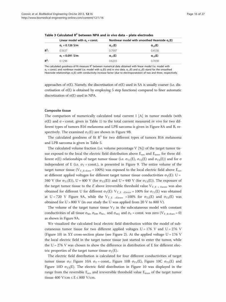
Table 3 Calculated R2 between NPA and in vivo data – plate electrodes

Linear model with σL = const. Nonlinear model with smoothed Heaviside σL(E)

σL = 0.126 S/m σL1(E) σL2(E)

R2: 0.5637 0.7997 0.4538

σL = 0.091 S/m σL1(E) σL2(E)

R2: 0.1296 0.6203 0.7838

The calculated goodness-of-fit measure R2 between numerical data obtained with linear model (i.e. model withσL = const.) and nonlinear model (i.e. model with σL(E)) and in vivo data. σL1(E) and σL2(E) stand for the smoothedHeaviside relationships σL(E) with conductivity increase factor (due to electroporatoion) of two and three, respectively.


approaches of σ(E). Namely, the discretisation of σ(E) used in SA is usually coarser (i.e. dis-

cretisation of σ(E) is obtained by employing 5 step functions) compared to finer automatic

discretization of σ(E) used in NPA.

Composite tissue

The comparison of numerically calculated total current I [A] in tumor models (with

σ(E) and σ = const. given in Table 1) to the total current measured in vivo for two dif-

ferent types of tumors B16 melanoma and LPB sarcoma is given in Figure 8A and B, re-

spectively. The examined σT(E) are shown in Figure 9B.

The calculated goodness of fit R2 for two different types of tumors B16 melanoma

and LPB sarcoma is given in Table 5.

The calculated volume fraction (i.e. volume percentage V [%]) of the target tumor tis-

sue exposed to the local the electric field distribution above Erev and Eirrev for three dif-

ferent σ(E) relationships of target tumor tissue (i.e. σT1(E), σT2(E) and σT3(E)) and for σ

independent of E (i.e. σT = const.), is presented in Figure 9. The entire volume of the

target tumor tissue (VT_E>Erev = 100%) was exposed to the local electric field above Erevat different applied voltages for different target tumor tissue conductivities σT(E): U =

340 V (for σT1(E)), U = 400 V (for σT2(E)) and U = 440 V (for σT3(E)). The exposure of

the target tumor tissue to the E above irreversible threshold value VT_E > Eirrev was also

obtained for different U for different σT(E): VT_E >Eirrev = 100% for σT1(E) was obtained

at U = 720 V Figure 9A, while the VT_E >Eirrev =100% for σT2(E) and σT3(E) was

obtained for U > 800 V (in our study the U was applied from 20 V to 800 V).

The volume of the target tumor tissue VT in the subcutaneous model with constant

conductivities of all tissue σSE, σDF, σM⊥ and σM|| and σT = const. was zero (VT_E>Erev = 0)

as shown in Figure 9A.

We visualized the calculated local electric field distribution within the model of sub-

cutaneous tumor tissue for two different applied voltages U = 176 V and U = 276 V

(Figure 10) in XY cross-section plane (see Figure 2). At the applied voltage U = 176 V

the local electric field in the target tumor tissue just started to enter the tumor, while

the U = 276 V was chosen to show the difference in distribution of E for different elec-

tric properties of the target tumor tissue σT(E).

The electric field distribution is calculated for four different conductivities of target

tumor tissue σT: Figure 10A σT = const., Figure 10B σT1(E), Figure 10C σT2(E) and

Figure 10D σT3(E). The electric field distribution in Figure 10 was displayed in the

range from the reversible Erev and irreversible threshold value Eirrev of the target tumor

tissue 400 V/cm ≤ E ≤ 800 V/cm.

Figure 6 Comparison of numerical simulations performed by IA to the data measured in vivo.Electric current vs. voltage relationships I(U) calculated in nonlinear models (with linear and exponential σL(E)), calculated in linear models (with σL(E) = σ0 = const.) and measured in vivo by using needle electrodeswith diameters: A. 0.3 mm, B. 0.7 mm and C. 1.1 mm.


Figure 7 Comparison of numerical simulations performed by IA, NPA and SA to the data measuredin vivo. A. Comparison of U(I) characteristics calculated in nonlinear model and linear to the in vivo data.B. The relationships σL(E) and constant conductivities σL(E) = σ0 = const. in nonlinear and linear models,respectively. The diameter of needle electrodes was 1.1 mm.


DiscussionIn a recent study of robustness of electrochemotherapy treatment planning based on

analysis of local electric field distribution E the authors show that the uncertainties in

predefined dielectric properties of the treated tissues and in the rate of increase in elec-

tric conductivity due to the electroporation have large effect on treatment effectiveness,

which indicated that more experimental and numerical research is needed [43]. Numer-

ous other numerical and experimental studies also showed that the electric conductivity

Table 4 Calculated R2 between IA, NPA and SA and in vivo data - needle electrodes

Electrode diameter

1.1 mm 0.7 mm 0.3 mm

Analysis type with σL(E) R2:

IA with linear σL(E) 0.883214 0.875605 0.92873

NPA with smoothed Heaviside σL(E) 0.9192

NPA with sigmoid σL(E) 0.8964

SA with sigmoid σL(E): 0.8938

* The calculated R2 for SA is given for the σL(E) with 5 discretization steps. The calculated R2 for models with σ beingindependent of E (σL = const. = 0.04593 S/m and σL = const. = 0.067 S/m) was negative.The calculated goodness-of-fit measure R2 between numerical data obtained with nonlinear model (model with σL(E))and in vivo data.

Figure 8 Numerically calculated vs. in vivo measured I(U) relationship in subcutaneous tumors.Comparison of numerically calculated I [A] (in both nonlinear and linear models) with the experimentallymeasured I [A] for two types of tumors: A. B16 melanoma and B. LPB sarcoma. In nonlinear numericalmodels we examined three different σL(E) of tumors (Table 1 and Figure 9b).


changes during tissue electroporation. However, in preclinical studies and clinical stud-

ies the electroporated tissues are often considered as conductive materials with con-

stant electric conductivities.

In our study we therefore investigated whether the functional dependency of electric

properties and of local electric field distribution within treated tissues need to be taken

into account when modeling tissue response to the electroporation pulses.

We compared linear (i.e. tissue conductivity is constant σ = const.) and non-linear

model (tissue conductivity depends on local electric field σ(E)) to the experimental data

in vivo [56]. We built our numerical models so as to fit as accurately as possible the tis-

sue geometry, the electrode geometry and the contact surface between the electrodes

and tissue treated in in vivo experiments. In the first part of our study we performed

the comparison for single tissue (i.e. one type of tissue) for two types of electrodes:

plate and needle electrodes. For single tissue modeling we analyzed the experimental

data performed in rat liver treated with plate electrodes and in rabbit liver treated with

needle electrodes (Figure 1).

Figure 9 Reversibly and irreversibly electroporated tumor volume VT [%] in linear (σT(E) = const.)and nonlinear models (σT (E)). A. The calculated percentage of tumor volume VT [%] exposed to the localelectric field above Erev and Eirrev and B. the examined baseline conductivities (σT(E) = const.) andrelationships σT(E) of the target tumor tissue.


The main findings of the single tissue analysis were then applied to the model of

composite tissue (i.e. the tissue composed of different types of tissues with different

electric conductivities). The study of composite tissue was performed for subcutaneous

tumor that consisted of stratum corneum, dermis, epidermis, connective and fatty tis-

sue, tumor tissue and muscle tissue and was treated with plate electrodes (Figure 2).

Numerical simulations in our study were performed by using three different model-

ing approaches: IA [60,61], NPA [62] and SA [58].

Table 5 Calculated R2 between model data and in vivo data (plate electrodes, NPA)

Tumor B16 Tumor LPB

Model R2: R2:

σT1(E) 0.4842 0.5197

σT2(E) 0.4992 0.4799

σT3(E) 0.5028 0.4322

* Subcutaneous tumor models with σ being independent of E (i.e. σT, σSE, σDF, σM⊥, σM|| = const.) have negative R2.The calculated goodness-of-fit measure R2 between numerical data obtained with nonlinear model (i.e. model with σ(E))and in vivo data obtained for B16 melanoma and LPB sarcoma.

Figure 10 Local electric field E in the numerical model of subcutaneous tumor. Calculated andvisualized local electric field E distribution for two different applied voltages U = 176 V and U = 276 V in XYcross section plane of the subcutaneous tumor model. The E is calculated for the following σT of the targettumor: A. σT = const., B. σT1(E), C. σT2(E) and D. σT3(E).


In our study the IA was first applied for numerical modeling of electroporation in a

single tissue (i.e. rat liver tissue) treated with plate electrodes. The relationship between

local electric field distribution and the conductivity of liver tissue σ(E) was described by

linear (Eq. 7) and exponential functions (Eq. 8). The parameters of these two functions

(parameters σ0 and kσ of linear function and parameters σ0, c1 and c2 of exponential

function) were than calculated with IA-analysis algorithm by fitting the data of numer-

ically calculated to the experimentally measured values of total electric current flowing

through the tissue (Figure 3). The parameters σ0 in both functions σ(E) (linear and ex-

ponential) represented the baseline tissue conductivities for the condition σ0 = σ(0))

(i.e. the initial conductivity of non-electroporated tissue). We calculated these parameters

to be σ0 = 0.088145 S/m (linear function Eq. 7) and σ0 = 0.092768 S/m (exponential func-

tion Eq. 8). The numerically calculated values of σ0 of both functions correspond well to

the measured conductivities of rat liver tissue published by Gabriel and colleagues [68].

These results show that the IA allows for identification of the initial tissue conductivity


based on measured values of total electric current flowing through the tissue exposed to

the electroporation pulses. In order to compare the numerical models of liver tissue that

consider exponential and linear σ(E) relationship to the numerical model with constant

conductivity (σ(E) = const.) we used the calculated data σ0 for development of the models

with constant conductivities: σ(E) = σ0 = const. The calculation of goodness of fit measure

(R2) of the numerical models that take into account the relationship σ(E) fit better experi-

mental data compared to the models with constant conductivity: linear σ(E) R2 = 0.7993

and exponential σ(E) R2 = 0.7995 vs. σ(E) = σ0 = 0.088145 S/m = const. R2 = 0.1295 and

σ(E) = σ0 = 0.092768 S/m = const. R2 = 0.1297 (Table 2)). These results show that the IA

also allows for identification of functional dependency of tissue conductivity σ(E) of the

electroporated tissue. The results of our study thus demonstrate that by using IA both the

baseline electric conductivity for non-electroporated tissue (for the condition σ(0) = const.

for E = 0 or E < Erev) and the σ(E) relationship of the tissue exposed to U that results in tis-

sue electroporation (E > Erev) can be identified.

The calculation of tissue conductance G [S] show that the conductance of the models

with σ(E) increased with increase of the applied voltage following the measured data of

G Figure 3D. We can observe that the models G = const. do not describe the electro-

poration process of the tissue which is in agreement with our previous findings [2,56],

as well as recent multiscale modeling [57].

In order to compare numerical simulations obtained by nonlinear parametric analysis

(NPA) to the numerical simulations obtained with inverse analysis (IA) we used the

same geometry of liver tissue and electrodes (Figure 1A) and electric properties of tis-

sue (σL0 = const. and σ(E)) as used in our previous work [62]. Namely, for the initial pa-

rameters of tissue conductivity we used two different measured values from the

literature σL0 = 0.091 S/m (pig liver) [68] and σL0 = 0.124 S/m (rat liver) [67]. The rela-

tionship between the local electric field and tissue conductivity σ(E) was implemented

to the tissue model as smoothed Heaviside’s function. The numerical calculations were

performed for both constant conductivity σ = const. and σ(E) with conductivity increase

factor of two and three (Figure 3B), which is in agreement with experimentally mea-

sured conductivity increase at the end of the pulse [2,58]. Our results show that the nu-

merical models with σ(E) better fit experimental data than models with σ = const.

(Table 3). Numerical model with initial conductivity of rat liver better fit experimental

data for the conductivity increase factor of two (R2 = 0.7997), the numerical model with

initial conductivity of pig liver better fit experimental data for the conductivity increase

factor of three (R2 = 0.7838). When comparing the numerical results obtained with

NPA to the results obtained with IA we can conclude that similar results and good

agreement between numerical and experimental data can be obtained with both model-

ing approaches when σ(E) relationship is taken into account (regardless of the shape of

the σ(E)). Both approaches show that the models with σ(E) fit the measured data con-

siderably better than models with constant conductivity. However, more precise mea-

surements are needed for determination of the shape of the σ(E) function that might be

tissue type specific.

In the second part of our study we built numerical models of single tissue (rabbit

liver) treated with needle electrodes of three different diameters 0.3 mm, 0.7 mm and

1.1, that were used also in in vivo experiments. By using IA we first identified the σ(E)

for the tissue model with needle electrodes with diameter of 0.7 mm, as in this case we


analyzed the maximum number of measurements Figure 6. We found that the best fit of

numerical data with experimental data was obtained with linear σ(E) function (Figure 6B)

with R2 = 0.875605 (Table 3). The identified value of the initial tissue conductivity was σ0 =

0.04593 S/m which correspond to the measured conductivity of rabbit liver (summarized in

[58]). The identified linear function in the model with 0.7 mm was then applied to the

models with 0.3 mm and 1.1 mm and good agreement between calculated data were

obtained R2 = 0.92873 (for 0.3 mm) and R2 = 0.883214 (for 1.1 mm) (Table 4).

For the model with electrode diameter 1.1 mm we also performed NPA with

smoothed Heaviside and sigmoid σ (E) function and sequential analysis with sigmoid

function σ(E) with parameters determined by [58]. We also performed numerical ana-

lysis with σ(E) = const. The comparison of the model with σ(E) = const. to the numer-

ical models with σ(E) showed that models with σ(E) fit experimental data considerably

better then models with σ(E) = const. (Table 4). When comparing numerical results of

different modeling approaches (Figure 7) we further observed that the best fit between

the numerical and experimental data was obtained with NPA with smoothed

Heaviside’s function R2 = 0.9192 (Table 4).

Based on the comparison of all three modeling approaches validated with experimen-

tal measurements we determined the important advantages for electroporation process

modeling of each of the approaches. Namely, the IA can be used as a modeling ap-

proach for the situations when the conductivity of treated tissue is difficult to be mea-

sured before or during electroporation. The NPA allows for parametric analysis of

electric current at the end of the applied voltage pulses while the SA allows also an

insight into the electroporation process (i.e. the course of σ(E) changes) during the ap-

plied pulse. Although, the NPA and SA modeling approaches require the baseline con-

ductivity and the σ(E) need to be predefined, the important advantage is that these two

modeling approaches are relatively simple to be used in commercial software which is

accessible and widely used.

In the third part of our study we built the numerical model of subcutaneous tumor

in order to examine the influence of tissue heterogeneity on the electric field distribu-

tion during electroporation of a composite tissue (i.e. tumor model composed of differ-

ent types of tissues). We compared the numerical calculation of total electric current in

the tumor model with constant conductivity of all constituent tissues and the numerical

calculation of total electric current in the tumor model that took into account σ(E) of

all involved tissues to the experimental measurements in vivo carried out in two differ-

ent types of tumors: B16 melanoma (Figure 8A) and LPB sarcoma (Figure 8B). For all

tissues in the model we implemented smoothed Heaviside’s function σ(E).

Based on the comparison of the numerical and experimental data in vivo we demon-

strated that the model that took into account σ(E) of all involved tissues fits better

in vivo data than model with constant conductivities (Table 5). Our results further

show that the subcutaneous tumor model with higher conductivity of target tumor tis-

sue σT3(E) fits better the in vivo data of B16 melanoma while the model with σT1(E)

better fits the in vivo data of LPB sarcoma subcutaneous tumor (Table 5), suggesting

that B16 melanoma has higher conductivity than LBP sarcoma. The visualization of

local E in the subcutaneous tumor model demonstrates that the more conductive the target

tumor tissue the higher the intensity of E in the surrounding tissue and the lower E in the

tumor tissue (Figure 10A and B), which is in agreement with our previous findings [70].


We also calculated the tumor volume exposed to the local electric field above Erevand Eirrev (Figure 9A) and demonstrated that more conductive target tumor tissue were

more difficult to be successfully electroporated, since they require higher voltage U to

be applied to the electrodes in order to expose the entire volume of the target tumor

above the Erev or higher, which also results in higher intensity of E in the skin and

muscle and subsequently may induce more damage to the surrounding healthy tissue

(Figure 10). We also demonstrated that the electroporation of more conductive tissues

resulted in higher values of total electric current I [A] flowing through tissue (Figure 8).

The exposure of the target tumor tissue to the E above irreversible threshold value also

depends on the electric properties of the target tumor tissue σT(E). It needs to be em-

phasized that the subcutaneous model with constant conductivities of all tissues (i.e. in

the subcutaneous tumor model that do not take into account the relationship σ(E))

showed that a very high electric field (E > Eirrev) was concentrated only in the stratum

corneum while the target tumor tissue was not treated (Figure 10A). Furthermore, the

volume of the target tumor tissue VT exposed to the E > Erev in the subcutaneous model

with constant conductivities of all tissue was zero (Figure 9A).

ConclusionsIn our study we investigated whether the increase in electric conductivity of tissues

needs to be taken into account when modeling tissue response to the electroporation

pulses and how it affects the local electric distribution within electroporated tissues.

We examined electric field distribution during electroporation in both linear models

(i.e. tissue conductivity is constant) and non-linear models (i.e. tissue conductivity is

electric field dependent). The results show that nonlinear models fit experimental

data better than linear models. We demonstrated that the tissue conductivity as a

function of electric field (i.e. σ(E)) needs to be considered when modeling tissue be-

havior during electroporation. Therefore, the σ(E) relationship needs to be taken into

account when an electroporation based treatment is planned or investigated. The

findings of our study can be of great importance for precise treatment planning of

electroporation based therapies and treatments (e.g. for electrochemotherapy, gene

electrotransfer for gene therapy and DNA vaccination, tissue ablation with irrevers-

ible electroporation and transdermal drug delivery). Particularly, for an electropor-

ation based therapy of deep-seated cutaneous tumors and tumors in internal organs,

such as for example bone, brain or muscle tissue that are surrounded by other tis-

sues having different electric properties an individualized patient-specific treatment

planning that takes into account heterogeneity of electric conductivity and local elec-

tric field distribution within all exposed tissues is required.

Competing interestsThe authors declare that they have no competing interests.

Authors’ contributionsSC and DM designed the study. PS, TS and TR performed modeling with IA. IL and SC performed modeling with NPA.SC performed modeling with SA. All authors were involved in the analysis of numerical and experimental data. Allauthors were involved in the preparing of the manuscript. All authors read and approved the final manuscript.

AcknowledgementThis work was supported by the Slovenian Research Agency and conducted within the scope of LEA EBAM (EuropeanAssociated Laboratory on the Electroporation in Biology and Medicine). This manuscript is a result of the networkingefforts of the COST Action TD1104 (http://www.electroporation.net). The authors thank Dr. David Cukjati for the resultsof in vivo experiments performed within his postdoctoral project.

http://www.electroporation.net/


Author details1University of Ljubljana, Faculty of Electrical Engineering, Trzaska cesta 25, SI-1000 Ljubljana, Slovenia. 2University ofZagreb, Faculty of Electrical Engineering and Computing, Unska 3, HR-10000, Zagreb, Croatia. 3C3M, d. o. o., Centre forComputational Continuum Mechanics, Technological Park 21, SI-1000 Ljubljana, Slovenia.

Received: 30 August 2012 Accepted: 10 December 2012Published: 21 February 2013

References
1. Neumann E, Schaefer-Ridder M, Wang Y, Hofschneider PH: Gene transfer into mouse lyoma cells by
electroporation in high electric fields. EMBO J 1982, 1:841–845.2. Pavlin M, Kanduser M, Rebersek M, Pucihar G, Hart FX, Magjarevic R, Miklavcic D: Effect of cell electroporation on

the conductivity of a cell suspension. Biophys J 2005, 88:4378–4390.3. Kotnik T, Pucihar G, Miklavcic D: Induced transmembrane voltage and its correlation with electroporation-mediated

molecular transport. J Membrane Biol 2010, 236:3–13.4. Pucihar G, Krmelj J, Rebersek M, Napotnik TB, Miklavcic D: Equivalent Pulse Parameters for Electroporation. IEEE

T Biomed Eng 2011, 58:3279–3288.5. Teissié J, Rols MP: An experimental evaluation of the critical potential difference inducing cell membrane

electropermeabilization. Biophys J 1993, 65(1):409–413.6. Cemazar M, Jarm T, Miklavcic D, Macek Lebar A, Ihan A, Kopitar NA, Sersa G: Effect of electric-field intensity on

electropermeabilization and electrosensitivity of various tumor-cell lines in vitro. Electro Magnetobiol 1998,17:263–272.

7. Valic B, Golzio M, Pavlin M, Schatz A, Faurie C, Gabriel B, Teissie J, Rols MP, Miklavcic D: Effect of electric field inducedtransmembrane potential on spheroidal cells: theory and experiments. Eur Biophys J 2003, 32:519–528.

8. Pucihar G, Kotnik T, Valic B, Miklavcic D: Numerical determination of transmembrane voltage induced onirregularly shaped cells. Annals Biomed Eng 2006, 34:642–652.

9. Corovic S, Zupanic A, Kranjc S, Al Sakere B, Leroy-Willig A, Mir LM, Miklavcic D: The influence of skeletal muscleanisotropy on electroporation: in vivo study and numerical modeling. Med Biol Eng Comput 2010, 48:637–648.

10. Prud’homme GJ, Glinka Y, Khan AS, Draghia-Akli R: Electroporation enhanced nonviral gene transfer for theprevention or treatment of immunological, endocrine and neoplastic diseases. Curr Gene Ther 2006, 6:243–273.

11. Miklavcic D, Beravs K, Semrov D, Cemazar M, Demsar F, Sersa G: The importance of electric field distribution foreffective in vivo electroporation of tissues. Biophys J 1998, 74:2152–2158.

12. Kotnik T, Bobanovic F, Miklavcic D: Sensitivity of transmembrane voltage induced by applied electric fields – atheoretical analysis. Bioelectrochem Bioenerg 1997, 43:285–291.

13. Miklavcic D, Corovic S, Pucihar G, Pavselj N: Importance of tumour coverage by sufficiently high local electricfield for effective electrochemotherapy. Eur J Cancer 2006, 4(Suppl):45–51.

14. Rols MP, Teissié J: Electropermeabilization of mammalian cells, Quantitative analysis of the phenomenon.Biophys J 1990, 58(5):1089–1098.

15. Miklavcic D, Semrov D, Mekid H, Mir LM: A validated model of in vivo electric field distribution in tissues forelectrochemotherapy and for DNA electrotransfer for gene therapy. Biochim Biophys Acta 2000, 1523:73–83.

16. Corovic S, Mir LM, Miklavcic D: In vivo muscle electroporation threshold determination: realistic numericalmodels and in vivo experiments. J Membrane Biol 2012, 245:509–520.

17. Davalos RV, Mir LM, Rubinsky B: Tissue ablation with irreversible electroporation. Ann Biomed Eng 2005, 33:223.18. Rubinsky J, Onik G, Mikus P, Rubinsky B: Optimal parameters for the destruction of prostate cancer using

irreversible electroporation. J Urol 2008, 180:2668–2674.19. Al-Sakere B, Andre F, Bernat C, Connault E, Opolon P, Davalos RV, Rubinsky B, Mir LM: Tumor ablation with

irreversible electroporation. PlosOne 2007, 2:1135.20. Vorobiev E, Lebovka N: Electrotechnologies for Extraction from Food Plants and Biomaterials. New York: Springer Science; 2008.21. Sack M, Sigler J, Frenzel S, Chr E, Arnold J, Michelberger T, Frey W, Attmann F, Stukenbrock L, Mueller G: Research

on Industrial-Scale Electroporation Devices Fostering the Extraction of Substances from Biological Tissue.Food Eng Rev 2010, 2:147–156.

22. Cemazar M, Tamzali Y, Sersa G, Tozon N, Mir LM, Miklavcic D, Lowe R, Teissie J: Electrochemotherapy inveterinary oncology. J Vet Intern Med 2008, 22(4):826–831.

23. Testori A, Tosti G, Martinoli C, Spadola G, Cataldo F, Verrecchia F, Baldini F, Mosconi M, Soteldo J, Tedeschi I,Passoni C, Pari C, Di Pietro A, Ferrucci PF: Electrochemotherapy for cutaneous and subcutaneous tumor lesions:a novel therapeutic approach. Dermatol Ther 2010, 23(6):651–661.

24. Cemazar M, Jarm T, Sersa G: Cancer electrogene therapy with interleukin-12. Curr Gene Ther 2010, 10(4):300–311.25. Heller LC, Heller R: Electroporation gene therapy preclinical and clinical trials for melanoma. Curr Gene Ther

2010, 10(4):312–317.26. Neal RE II, Rossmeisl JH Jr, Garcia PA, Lantz O, Henao-Guerrero N, Davalos RV: Successful treatment of a large

soft-tissue sarcoma with irreversible electroporation. J Clin Oncol 2011, 29(13):372–377.27. Sersa G, Cufer T, Paulin Kosir S, Cemazar M, Snoj M: Electrochemotherapy of chest wall breast cancer

recurrence. Cancer Treat Rev 2012, 38(5):379–386.28. Morales-de La Peña M, Elez-Martínez P, Martín-Belloso O: Food preservation by pulsed electric fields: an

engineering perspective. Food Eng Rev 2011, 3:94–107.29. Rieder A, Schwartz T, Schön-Hölz K, Marten SM, Süß J, Gusbeth C, Kohnen W, Swoboda W, Obst U, Frey W:

Molecular monitoring of inactivation efficiencies of bacteria during pulsed electric field (PEF) treatment ofclinical wastewater. J Appl Microbiol 2008, 105:2035–2045.

30. Campana LG, Valpione S, Mocellin S, Sundararajan R, Granziera E, Sartore L, Chiarion-Sileni V, Rossi CR:Electrochemotherapy for disseminated superficial metastases from malignant melanoma. BJS 2012, 99:821–830.


31. Pech M, Janitzky A, Wendler JJ, Strang C, Blaschke S, Dudeck O, Ricke J, Liehr UB: Irreversible electroporation ofrenal cell carcinoma: a first-in-man phase I clinical study. Cardiovasc Intervent Radiol 2011, 34(1):132–138.

32. Onik G, Rubinsky B: Irreversible electroporation: First patient experience—Focal therapy of prostate cancer. InIrreversible Electroporation. Edited by Rubinsky B. Heidelberg, Germany: Springer Berlin; 2010:235–247.

33. Daud AI, DeConti RC, Andrews S, Urbas P, Riker AI, Sondak VK, Munster PN, Sullivan DM, Ugen KE, Messina JL,Heller R: Phase I trial of interleukin-12 plasmid electroporation in patients with metastatic melanoma. J ClinOncol 2008, 26:896–903.

34. Ahmad S, Casey G, Sweeney P, Tangney M, O'Sullivan GC: Optimized electroporation mediated DNAvaccination for treatment of prostate cancer. Genet Vaccines Ther 2010, 8:1.

35. Mir LM: Bases and rationale of the electrochemotherapy. EJC 2006, 4(Suppl):38–44.36. Campana LG, Mocellin S, Basso M, Puccetti O, De Salvo GL, Chiarion-Sileni V, Vecchiato A, Corti L, Rossi CR, Nitti D:

Bleomycin-based electrochemotherapy: clinical outcome from a single institution's experience with 52patients. Ann Surg Oncol 2009, 16(1):191–199.

37. Matthiessen LW, Chalmers RL, Sainsbury DC, Veeramani S, Kessell G, Humphreys AC, Bond JE, Muir T, Gehl J:Management of cutaneous metastases using electrochemotherapy. Acta Oncol 2011, 50(5):621–629.

38. Gargiulo M, Papa A, Capasso P, Moio M, Cubicciotti E, Parascandolo S: Electrochemotherapy for non-melanomahead and neck cancers: clinical outcomes in 25 patients. Ann Surg 2012, 255(6):1158–1164.

39. Miklavcic D, Snoj M, Zupanic A, Kos B, Cemazar M, Kropivnik M, Bracko M, Pecnik T, Gadzijev E, Sersa G: Towards treatmentplanning and treatment of deep-seated solid tumors by electrochemotherapy. Biomed Eng Online 2010, 9:10.

40. Edhemovic I, Gadzijev EM, Brecelj E, Miklavcic D, Kos B, Zupanic A, Mali B, Jarm T, Pavliha D, Marcan M, Gasljevic G,Gorjup V, Music M, Pecnik Vavpotic T, Cemazar M, Snoj M, Sersa G: Electrochemotherapy: A new technologicalapproach in treatment of metastases in the liver. Technol Cancer Res Treat 2011, 10:475–485.

41. Corovic S, Al-Sakere B, Haddad V, Miklavcic D, Mir LM: Importance of contact surface between electrodes andtreated tissue in electrochemotherapy. Technol Cancer Res Treat 2008, 7:393–400.

42. Ivorra A, Al-Sakere B, Rubinsky B, Mir LM: Use of conductive gels for electric field homogenization increases theantitumor efficacy of electroporation therapies. Phys Med Biol 2008, 53:6605–6618.

43. Kos B, Zupanic A, Kotnik T, Snoj M, Sersa G, Miklavcic D: Robustness of treatment planning forelectrochemotherapy of deep-seated tumors. J Membrane Biol 2010, 236:147–153.

44. Pavliha D, Kos B, Zupanic A, Marcan M, Sersa G, Miklavcic D: Patient-specific treatment planning ofelectrochemotherapy: Procedure design and possible pitfalls. Bioelectrochemistry 2012, 87:265–273.

45. Fini M, Tschon M, Alberghini M, Bianchi G, Mercuri M, Campanacci L, Cavani F, Ronchetti M, De Terlizzi F, Cadossi R:Cell electroporation in bone tissue. In Clinical aspects of electroporation. Edited by Kee ST, Gehl J, Lee EW. New York:Springer; 2011:115–127.

46. Agerholm-Larsen B, Iversen HK, Ibsen P, Moller JM, Mahmood F, Jensen KS, Gehl J: Preclinical validation ofelectrochemotherapy as an effective treatment for brain tumors. Cancer Res 2011, 71(11):3753–3762.

47. Garcia PA, Pancotto T, Rossmeisl JH, Henao-Guerrero N, Gustafson NR, Daniel GB, Robertson JL, Ellis TL, Davalos RV:Non-Thermal Irreversible Electroporation (N-TIRE) and Adjuvant Fractionated Radiotherapeutic MultimodalTherapy for Intracranial Malignant Glioma in a Canine Patient. Technol Cancer Res Treat 2011, 10:73–83.

48. Corovic S, Zupanic A, Miklavcic D: Numerical modeling and optimization of electric field distribution in subcutaneoustumor treated with electrochemotherapy using needle electrodes. IEEE T Plasma Sci 2008, 36:1665–1672.

49. Zupanic A, Corovic S, Miklavcic D: Optimization of electrode position and electric pulse amplitude inelectrochemotherapy. Radiol Oncol 2008, 42:93–101.

50. Zupanic A, Corovic S, Miklavcic D, Pavlin M: Numerical optimization of gene electrotransfer into muscle tissue.Biomed Eng Online 2010, 9:66.

51. Zupanic A, Miklavcic D: Optimization and numerical modeling in irreversible electroporation treatmentplanning. In Irreversible Electroporation. Edited by Rubinsky B. Heidelberg: Springer; 2010:203–222.

52. Neal RE II, Garcia PA, Robertson JL, Davalos RV: Experimental characterization and numerical modeling of tissueelectrical conductivity during pulsed electric fields for irreversible electroporation treatment planning. IEEE TBiomed Eng 2012, 59(4):1077–1085.

53. Garcia PA, Rossmeisl JH, Neal RE, Ellis TL, Olson JD, Henao-Guerrero N, Robertson J, Davalos RV: IntracranialNonthermal Irreversible Electroporation: In Vivo Analysis. J Membr Biol 2010, 236:127–136.

54. Mahmood F, Gehl J: Optimizing clinical performance and geometrical robustness of a new electrode devicefor intracranial tumor electroporation. Bioelectrochemistry 2011, 81:10–16.

55. Zupanic A, Kos B, Miklavcic D: Treatment planning of electroporation-based medical interventions:electrochemotherapy, gene electrotransfer and irreversible electroporation. Phys Med Biol 2012, 57:5425–5440.

56. Cukjati D, Batiuskaite D, André F, Miklavčič D, Mir LM: Real time electroporation control for accurate and safein vivo non-viral gene therapy. Bioelectrochemistry 2007, 70:501–507.

57. Essone Mezeme M, Pucihar G, Pavlin M, Brosseau C, Miklavcic D: A numerical analysis of multicellularenvironment for modeling tissue electroporation. Appl Phys Lett 2012, 100:143701.

58. Sel D, Cukjati D, Batiuskaite D, Slivnik T, Mir LM, Miklavcic D: Sequential finite element model of tissueelectropermeabilization. IEEE Trans Biomed Eng 2005, 52:816–27.

59. Pavselj N, Bregar Z, Cukjati D, Batiuskaite D, Mir LM, Miklavcic D: The course of tissue permeabilization studiedon a mathematical model of a subcutaneous tumor in small animals. IEEE Trans Biomed Eng 2005, 52:1373.

60. Gresovnik I: A General Purpose Computational Shell for Solving Inverse and Optimisation Problems - Applications toMetal Forming Processes. PhD Thesis: University of Wales Swansea, UK; 2000.

61. Center for Computational Continuum Mechanics (Ljubljana, Slovenia).; [www.c3m.si].62. Lackovic I, Magjarevic R, Miklavcic D: Incorporating Electroporation-related conductivity changes into models

for the calculation of the electric field distribution in tissue. In Proceedings of IFMBE (XII MediterraneanConference on Medical and Biological Engineering and Computing). Edited by Magjarevic R, Bamidis Panagiotis D,Pallikarakis N. Berlin Heidelberg: Springer; 2010:695–698.

http://www.c3m.si/


63. Giavazzi S, Ganatea MF, Trkov M, Sustarsic P, Rodic T: Inverse determination of viscoelastic properties of humanfingertip skin. Materials and Geoenvironment 2010, 57:1–16.

64. Korelc J: AceGEN (Multi-language, Multi-environment Numerical Code Generation) – Users manual.; 2009 [http://www.fgg.uni-lj.si/symech/].

65. Korelc J: AceFEM ((The Mathematica Finite Element Environment) – Users manual.; 2009 [http://www.fgg.uni-lj.si/symech/].66. Korelc J: Automation of primal and sensitivity analysis of transient coupled problems. Comput Mech 2009,

44:631–649.67. Haemmerich D, Staelin ST, Stai JZ, Tungjitkusolmun S, Mahvi DM, Webster JG: In vivo electrical conductivity of

hepatic tumours. Physiol Meas 2003, 24:251–260.68. Gabriel C, Peyman A, Grant EH: Electrical conductivity of tissue at frequencies below 1 MHz. Phys Med Biol 2009,

54:4863–4878.69. Pavselj N, Miklavcic D: A numerical model of permeabilized skin with local transport regions. IEEE T Biomed Eng

2008, 55:1927–1930.70. Corovic S, Pavlin M, Miklavcic D: Analytical and numerical quantification and comparison of the local electric

field in the tissue for different electrode configurations. Biomed Eng Online 2007, 6:37.

doi:10.1186/1475-925X-12-16Cite this article as: Corovic et al.: Modeling of electric field distribution in tissues during electroporation.BioMedical Engineering OnLine 2013 12:16.

Submit your next manuscript to BioMed Centraland take full advantage of:

• Convenient online submission

• Thorough peer review

• No space constraints or color figure charges

• Immediate publication on acceptance

• Inclusion in PubMed, CAS, Scopus and Google Scholar

• Research which is freely available for redistribution

Submit your manuscript at www.biomedcentral.com/submit

http://www.fgg.uni-lj.si/symech/



Documents

Modeling of electric field distribution in tissues during ...lbk.fe.uni-lj.si/pdfs/be2013sc.pdf · Modeling of electric field distribution in tissues during electroporation Selma