Modeling of fractured producer and injection in low

$Page 1: Modeling of fractured producer and injection in low$
Modeling of fractured producer and injection in low permeability reservoir

Marina Sacramento Salamanca

Petroleum Engineering

Supervisor: Jon Kleppe, IPTCo-supervisor: Per Arne Slotte, IPT

Håkon Høgstøl, IPT

Department of Petroleum Engineering and Applied Geophysics

Submission date: July 2013

Norwegian University of Science and Technology


NTNU

Norges teknisk-naturvitenskapelige Fakultet for ingeniørvitenskap og

teknologi

universitet

Faculty of Engineering and

Technology

Studieprogram i Geoffag og petroleumsteknologi

Study Programme in Earth Sciences and Petroleum Engineering

Institutt for petroleumsteknologi og anvendt geofysikk

Department of Petroleum Engineering and Applied Geophysics

Kandidatens navn/ The candidate’s name: Marina Salamanca

Oppgavens tittel, engelsk/Title of Thesis, English. Modeling of fractured producer and injection

well in low permeability reservoir

Utfyllende tekst/Extended text:

1.

2.

Studieretning/Area of specialization: Reservoir Engineer

Fagområde/Combination of subjects: Reservoir Engineer

Tidsrom/Time interval: January to July, 2013

________Jon Kleppe________

Faglærer/Teacher

Original: Student

Kopi: Fakultet

Kopi:Institut

i

Acknowledgements

Writing this thesis has been a challenging, exciting and outmost educational process which has

given me the opportunity to do the practical work of a reservoir engineer. However, this thesis

could never have been completed without help and support from the following:

The grace of God for one more opportunity.

I am heartily thankful to my supervisor at Statoil Håkon Høgstøl and Per Arne Slotte, for the time

and attention provided to guide this work.

Professor at Jon Kleppe by NTNU for the material offered.

I would like to thank Statoil ASA (Trondheim) for support and for infrastructure offered.

To all my family, especially parents, sisters and brothers for the love, care and support in a

challenging phase of my life.

I offer my best regards and blessings to all my friends who supported and encouraged me in any

respect during the completion of the project. Anyway, to all who contributed to realization of this

project my sincere thanks.

ii

Abstract

Hydraulic fracturing is one of the well-established well stimulation techniques for low

permeability reservoir. Hence, considerable amount of effort has been devoted to study their

performance under different conditions. This work presents a study modeling of fractured

production and injector well in low permeability reservoir. In this work, the simulator ECLIPSE

and REVEAL are used, to investigate and analyzing the impact of various factors in predicting the

behavior of these reservoirs. This study was divided in two parties. The first was to create

hydraulics fractures in reservoir simulation model using local grid refinement, skin factor and

conductivity fractures in eclipse and compare with analytical solution. The results demonstrate that

for a vertical well having a vertical fracture, skin factor method seems to be sufficient as it offers

acceptable accuracy, high computational efficiency, and simplicity to apply. For horizontal wells,

however, skin factor method can significantly under-estimate well productivity and should not be

used. LGR method can be used for both vertical and horizontal wells with good accuracy, but CPU

time can be too high. For conductivity fractures the results indicate that this method is very good

when the fracture extend over several grid cell for vertical well. The second part developed a

method to model fractures generated by water injection above the fracture pressure in the

Simulator Reveal. We present a model to predict the initation and growth of a fracture in near

wellbore region due to the combined influence of injection pressure, thermal stresses due to

injection of cold water and an additional fracture pressure drop due to particles plugging. The

results indicate that injection of cold water into a high temperature reservoir induces thermal

stresses in the near wellbore region, which facilitate fracturing. It is found that at a given injection

rate an increase in plugging leads to significant increases in fracture half length.

iii

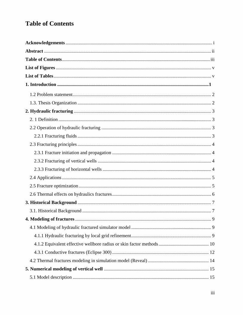
Table of Contents

Acknowledgements ........................................................................................................................... i

Abstract ............................................................................................................................................ ii

Table of Contents ............................................................................................................................ iii

List of Figures .................................................................................................................................. v

List of Tables .................................................................................................................................... v

1. Introduction ............................................................................................................................... 1

1.2 Problem statement .................................................................................................................... 2

1.3. Thesis Organization ................................................................................................................ 2

2. Hydraulic fracturing ................................................................................................................... 3

2. 1 Definition ................................................................................................................................ 3

2.2 Operation of hydraulic fracturing ............................................................................................ 3

2.2.1 Fracturing fluids ................................................................................................................ 3

2.3 Fracturing principles ................................................................................................................ 4

2.3.1 Fracture initiation and propagation ................................................................................... 4

2.3.2 Fracturing of vertical wells ............................................................................................... 4

2.3.3 Fracturing of horizontal wells ........................................................................................... 4

2.4 Applications ............................................................................................................................. 5

2.5 Fracture optimization ............................................................................................................... 5

2.6 Thermal effects on hydraulics fractures ................................................................................... 6

3. Historical Background ................................................................................................................ 7

3.1. Historical Background ............................................................................................................ 7

4. Modeling of fractures .................................................................................................................. 9

4.1 Modeling of hydraulic fractured simulator model ................................................................... 9

4.1.1 Hydraulic fracturing by local grid refinement ................................................................... 9

4.1.2 Equivalent effective wellbore radius or skin factor methods .......................................... 10

4.3.1 Conductive fractures (Eclipse 300) ................................................................................. 12

4.2 Thermal fractures modeling in simulation model (Reveal) ................................................... 14

5. Numerical modeling of vertical well ........................................................................................ 15

5.1 Model description .................................................................................................................. 15

iv

5.2. Local grid refinement method ............................................................................................... 16

5.2.2 Data included in numerical model .................................................................................. 17

5. 3 Verification of numerical model (Analytical solution) ......................................................... 21

5.4 Skin factor method ................................................................................................................. 22

5.4.1 Skin factor vs LGR .......................................................................................................... 24

5.5. Vertical well for heterogeneous reservoirs ........................................................................... 30


5.6 Conductive fractures (Eclipse 300) ........................................................................................ 36

5.6.1 LGR vs Conductive fractures (Eclipse 300) ................................................................... 38

5.7 Sensivity analyses .................................................................................................................. 40

5.7.1 Scenario 1: Non-fractured wells ...................................................................................... 40

5.7.2 Scenario 2: fractured wells .............................................................................................. 42

6. Numerical modeling of horizontal well .................................................................................... 47

6.1. Numerical Modeling Methodology ....................................................................................... 47


6.1.2 LGR vs Conductive fractures (Eclipse 300) ................................................................... 50

6.1.3 Scenario 3: Number fractured wells ................................................................................ 51

7. Thermal fractures ...................................................................................................................... 52

7.1 Modeling fracture growth in injection well ........................................................................... 52

7.1.2 Effect of particle plugging ............................................................................................... 53

7.1.3 Effect of flow rate ........................................................................................................... 57

8. Summary and Recommendations ............................................................................................ 61

8.1. Summary ............................................................................................................................... 61

References ....................................................................................................................................... 63

Nomenclature ................................................................................................................................. 66

Appendix A Simulation cases ....................................................................................................... 68

A.1 Example on Eclipse LGR set-up for a vertical well .............................................................. 68

A.2 Example on Eclipse LGR set-up for a horizontal well ......................................................... 75

v

List of Figures

Figure 1: Vertical fracture around a vertical well (Fjaer et al. 2008). .................................................... 4

Figure 2: Longitudinal (left) and transverse (right) hydraulic fractures in horizontal wells (Soliman,

et al. 1990). ..................................................................................................................................................... 5

Figure 3: Example of gradual Cartesian LGR ........................................................................................... 9

Figure 4: Schematic drawing of the skin factor ....................................................................................... 11

Figure 5: Example of one grid block (A) and several grid (B) Cartesian conductivity fractures. .... 13

Figure 6: The simulation grid of the sector model in Eclipse for a vertical well. ............................... 15

Figure 7: Oil production rate and Computer simulation time for wellbore LGR sensitivity analysis.

....................................................................................................................................................................... 17

Figure 8: Fracture and wellbore LGR used in the model. ...................................................................... 18

Figure 9: Comparison of refined 5x5 LGR with real fracture width vs. “coarse” 5x5 LGR with 2 ft

for the fracture ( = 200 ft, conductivity of 2000 mD-ft). .................................................................. 19

Figure 10: LGR of for a short vertical fracture of 75 ft half-length (global grid cell size is 400 ft).

.................................................................................................................................................................... 20

Figure 11: LGR of for a vertical fracture of 400 ft half-length (global grid cell size is 400 ft). ....... 20

Figure 12: Oil production total model simulation results with analytical solution for finite

conductivity type curve for constant pressure case. ............................................................................... 22

Figure 13: Comparison of results from skin factor method with those from LGR method. The green line is

for LGR method. The blue line is for skin factor method for a half-length 75 and hydraulic fracture of 2000

mD-ft conductivities. ..................................................................................................................................... 25

Figure 14: Comparison of results from skin factor method with those from LGR method. The green

line is for LGR method. The light blue line is for skin factor method for a half-length is 200 and

hydraulic fracture of 2000 mD-ft conductivities. .................................................................................... 26





line is for LGR method. The blue line is for skin factor method for a half-length is 400 and



line is for skin factor method. The light blue line is for LGR method for a half-length is 600 and


Figure 18: Comparison of results from skin factor method to those from LGR method for

heterogeneous reservoir for a half-length is 75 and hydraulic fracture of 2000 mD-ft

conductivities. .............................................................................................................................................. 31

Figure 19: Comparison of results from skin factor method with those from LGR method for


conductivities. .............................................................................................................................................. 32

vi



conductivities. .............................................................................................................................................. 33



conductivities. .............................................................................................................................................. 34



conductivities. .............................................................................................................................................. 35

Figure 23: conductivity fractures for vertical fracture of 200 ft half-length (global grid cell size is

400 ft). ........................................................................................................................................................... 36

Figure 24: Conductivity fractures for vertical fracture of 600 ft half-length (global grid cell size is

400 ft). ........................................................................................................................................................... 37

Figure 25: Comparison of results of the base case from Eclipse 100 and 300 without fractures .... 37

Figure 26: Comparison of results from conductivity fractures method with those from LGR

method. The green line is for conductive fractures method the light blue line is for LGR method

for a half-length is 200 and hydraulic fracture of 2000 mD-ft conductivities. ................................... 38

Figure 27: Comparison of results from conductivity fractures method with those from LGR

method. The green line is for conductive fractures method the light blue line is for LGR method

for a half-length is 600 and hydraulic fracture of 2000 mD-ft conductivities. ................................... 39

Figure 28: Oil production rate from a vertical well for local grid refinement methods values. For

base case without fractures is green line of the light blue is with fractures. ....................................... 41

Figure 29: Oil production rate from a vertical well of different skin values. The green line denotes

the case of skin 0, the blue line is for the case skin of -4. ...................................................................... 42

Figure 30: Oil production rate from a vertical well of different fracture conductivity values. The

light blue line denotes the case of 10000 conductivity fractures. The blue line is for the case of

conductivity fractures of 2000. The green line is the case for conductivity fractures of 1000. ........ 43

Figure 31: Oil production rate from a vertical well of different rock permeabilities. For the case of

fracture conductivity of 2000 and half-length of 200 ft. ........................................................................ 44

Figure 32: Oil production rate from a vertical well of different half lengths values. For local grid

refinement methods. .................................................................................................................................... 45

Figure 33: Oil production rate from a vertical well of different half lengths values. For skin factor

methods ......................................................................................................................................................... 46

Figure 34: Locations of the transverse hydraulic fractures of the horizontal well modeled by using

LGR. For a transverse fracture of 200 ft half-length. ............................................................................. 47

Figure 35: Comparison of refined 5x5 LGR with real fracture width vs. “coarse” 5x5 LGR with 2

ft for horizontal well with fracture ( = 200 ft, conductivity of 2000 mD-ft). ................................. 48

Figure 36: Comparison of oil production from cases when the hydraulic fractures are modeled

using skin factor and using LGR. The lines in green are for the skin of -3 case; the lines in blue is

for the LGR case. ........................................................................................................................................ 49

vii

Figure 37: Comparison of oil production from cases when the hydraulic fractures are modeled

using conductivity fracture methods and LGR methods. The lines in green are for the conductive

fracture and the line in blue is for the LGR case. ................................................................................... 50

Figure 38: Comparison of oil production for one to three longitudinal fractures in horizontal well

for the case conductivity fracture 2000 mD-ft and half-length 200 ft. ................................................ 51

Figure 39: Plan view of a growing two-winged fracture in simulator ................................................ 53

Figure 40: Effect of injected particle concentration on fracture growth with time. .......................... 54

Figure 41: Effect of injected particle concentration on water cut. ...................................................... 55

Figure 42: Effect of injected particle concentration on oil produced. ................................................. 56

Figure 43: Effect of flow rate on fracture length. .................................................................................. 57

Figure 44: Effect of flow rate on water cut ............................................................................................. 58

Figure 45: Effect of flow rate on oil produced ....................................................................................... 59

Figure 46: Comparison oil production rate performance from simulation cases using Eclipse and

Reveal software ........................................................................................................................................... 60

viii

List of Tables

Table 1: Representation hydraulic fracturing in eclipse by the method LGR .................................... 10

Table 2: Representation hydraulic fracturing in Eclipse 300 by the method CONDFRAC ............ 13

Table 3: Summary of input parameters for homogeneous reservoir. .................................................. 15

Table 4: Sensitivity analyses for wellbore LGR determination. .......................................................... 16

Table 5: Input permeabilities for different fracture conductivities assuming the fracture width of

0.5 in ............................................................................................................................................................. 18

Table 6: values used for calculate the skin stimulation formulas ........................................................ 23

Table 7: Input skin factor for different fracture conductivities ............................................................ 24

Table 8: Summary of input parameters for the single well simulations. ............................................ 52

Modeling of fractured producer and injection well in low permeability reservoir

Marina Salamanca 1

1. Introduction

Operations of stimulation are interventions or operations well in order to increase their

productivity, establishing channels of high conductivity for fluid flow, increasing the permeability

of the original rock, thus facilitating fluid flow from the rock to the well (Clark J. B, 1949). There

are many stimulation operations, but this work will study specifically only the technique of

hydraulic fracturing that is the stimulation operation most used for low permeability reservoirs.

This has motivated the development of several studies aimed at improving the technique of

hydraulic fracturing and solution of some problems related to it.

Hydraulic fracturing technology is the creation of fractures within a reservoir that contains oil or

natural gas in order to increase flow and maximize production. A hydraulic fracture is formed

when a fluid is pumped down the well at pressures that exceed the rock strength, causing open

fractures to form in the rock. Low permeability reservoirs, as well as many moderate permeability

reservoirs, often require hydraulic fracturing.

Prediction of reservoir and well behavior require numerical simulation, as do some of the more

complex problems of optimization. Using numerical analysis or new semi-analytic solutions,

production forecasts can be obtained for various development scenarios then economics can be

calculated for optimizing well spacing and hydraulic fracture length. Formation permeability is a

key technical criterion because higher permeability wells are able to drain much larger areas.

Lower permeability wells require longer hydraulic fractures and closer well spacing.


Marina Salamanca 2

1.2 Problem statement

The objective of this work was to compare different ways of representing hydraulics fractures in

reservoir simulation model of low permeability reservoir. The following topics were analyzed:

Implementation of the different methods for modeling fractures in simulation model such

as local grid refinement, effective wellbore radius and conductivity fracture using simulator

eclipse, for vertical and horizontal production well for homogenous and layered reservoirs

and compare with analytical solution.

Analyze the parameters that affect the behavior of hydraulics fractures.

Developments of the method for modeling fractures generated by water injection above the

fracture pressure in the simulator reveal. The factors that influence the growth of the

fracture such as, temperature and rock fracture plugging were also analyzed.

1.3. Thesis Organization

This report consists of eight chapters.

Chapter 1 is introduction to the work, gives a brief description of the hydraulics fracturing its

importance and usefulness.

Chapter 2 exposes the theoretical framework of hydraulics fracturing by definition, and

applications. In this chapter, the concepts necessary for understanding of the published work in

this area are presented.

Chapter 3 a basic introduction to the hydraulic fracturing process and the fundamental mechanics is

given. Main methods to simulate hydraulically fractured vertical and horizontal wells and past work on

the subject is investigated.

Chapter 4 presents the development of the numerical model in simulator model.

Chapter 5 presents the development of the numerical model for vertical well, numerical simulation

process and verification of the numerical model which was provided also the strategies that have been

implemented to exchange some parameters.

Chapter 6 describes study numerical model for horizontal well, numerical simulation results.

Chapter 7 presents the development of the numerical model for fractures generated by water injection.

Chapter 8 presents summary of the complete investigation with recommendations for the future work.


Marina Salamanca 3

2. Hydraulic fracturing

2. 1 Definition

Consists of the injection of a fluid in formation under a pressure high enough to cause breakage of

the rock. The injected fluids contain granular materials which are responsible for the maintenance

of fracture generated, then creating channels high permeability (Ghalambor, 2009).

2.2 Operation of hydraulic fracturing

The hydraulic fracturing process for reservoir stimulation involves heavy pumping of a fracturing

fluid down the well at larger rates than the rate of fluid escape into the formation. Thereby, the

hydraulic effect exceeds the strength of the formation and a fracture is created. Consequently, the

fracturing fluid disappears into the formation through the fracture. If the pump rate is kept larger

than the rate of fluid loss, the fracture will propagate further into the formation and increase the

wellbore contact area with the formation. When pumping ceases, the fracture will close and no

further effect would be seen. To prevent this from happening, a highly resistant material, called

proppants, is injected together with the fluid. This creates porosity in the fracture as well as

sufficient fracture conductivity. After the proppants have been placed, the pressure is relieved and

the well is shut in for a period. The shut- in period allows the fracture to close around the

proppants and for the injected fluid to leak off. Afterwards, the fracture has gained properties

important for reservoir flow and production enhancement.

2.2.1 Fracturing fluids

During stimulation by hydraulic fracturing fluid is injected into the wellbore at high pressures to

create and extend a fracture in the formation. Two methods of transporting the proppants in the

fluid are used – high-rate and high-viscosity. High-viscosity fracturing tends to cause large

dominant fractures, while with high-rate fracturing causes small spread-out micro-fractures

(Ghalambor, 2009).

To achieve successful stimulation, the fracturing fluid must have certain physical and chemical

properties:

It should have Good transport capacity.

Low loss of fluid formation.

Be compatible with the material and the formation fluid.

Should be easily removed in the formation.

It should be capable of suspending proppants and transporting them deep into the fracture.

It should be capable, through its inherent viscosity, to develop the necessary fracture width

to accept proppants.

http://en.wikipedia.org/wiki/Viscosity


Marina Salamanca 4

2.3 Fracturing principles

2.3.1 Fracture initiation and propagation

The fractures always propagate in a symmetric plane, directed perpendicular to the minimum in-

situ stress (Economides et al. 2000). Commonly this stress is horizontal, creating a vertical

fracture. For other cases, for instance where the vertical overburden stress component is the least

in-situ stress, the fracture becomes horizontal. Fracture initiation, however, occurs in the direction

of least resistance, which is not necessarily directed perpendicular to the minimum in-situ

horizontal stress. In horizontal or deviated boreholes initial fracture direction depends on the

wellbore azimuth. Wellbores with azimuths oriented parallel and perpendicular to the minimum in-

situ stress create fractures normal and parallel to the wellbore, respectively. If the wells are not in

alignment to the horizontal stresses, fractures will initiate in the direction of least resistance, which

may seem random. Further out in the formation, the fractures locate the in-situ stress, re-orientate

and propagate according to the general rule. (Fjaer et al. 2008).

2.3.2 Fracturing of vertical wells

As depth increases, overburden stress in the vertical direction increases. As the stress in the

vertical direction becomes greater with depth, the overburden stress (stress in the vertical

direction) becomes the greatest stress. Thus the least stress is represented by the smallest

horizontal stress and the induced fracture will be perpendicular to this stress, or in the vertical

orientation (Fjaer et al. 2008).

Since hydraulically induced fractures are formed in the direction perpendicular to the least stress,

as depicted in Figure 1, the resulting fracture would be oriented in the vertical direction.

Figure 1: Vertical fracture around a vertical well (Fjaer et al. 2008).

2.3.3 Fracturing of horizontal wells

The type of hydraulic fracture created is dependent on the azimuthal direction of the wellbore. The

geometry of fractures initiated from horizontal wells will depend on in-situ stresses. Reservoir

rocks are subjected to three mutually orthogonal in-situ stresses: the vertical stress (σv); the

maximum horizontal stress (σH); and the minimum horizontal stress (σh). Two limiting wellbore-

fractures have received considerable interest a (Valko et al. 1995):


Marina Salamanca 5

Longitudinal fractures are those that propagate in planes parallel with wellbore axes, they

form where horizontal wells are drilled parallel with the larger of the horizontal stresses or

parallel with the preferred fracture plane, as showing the figure 2 in the left.

Transverse fractures propagate in planes orthogonal to wellbore axes; they form where

horizontal wells are drilled perpendicular to the larger of the horizontal stresses or

perpendicular to the preferred fracture plane, as showing the figure 2 in the right.

Figure 2: Longitudinal (left) and transverse (right) hydraulic fractures in horizontal wells (Soliman,

et al. 1990).

2.4 Applications

There are many applications for hydraulic fracturing, (Lake et al. 2007):

Increase the drainage area between a formation and wellbore.

Connect the natural fractures.

Increase the flow rate of hydrocarbons produced from the low permeability reservoirs or

wells that have been damaged.

Connect the full vertical extent of a reservoir to a horizontal well.

2.5 Fracture optimization

Increased production operation by hydraulic fracturing will be a function of the length of the

fracture, fracture thickness and positive contrast between the permeability of the supporting agent

in the fracture and the permeability of the formation. The fracture conductivity is a measure of

how easily fluid moves through a fracture. It is defined as the product of fracture permeability and

fracture width as shown equation 2.1.


Marina Salamanca 6

When the value of flow capacity is divided by product of formation permeability (k) and fracture

half length (xf), the results is known as the dimensionless fracture conductivity defined as equation

2.2:

This ratio, Fcd, must be large to have a substantive, long-term increase in production. For low

permeability formations, the denominator becomes small, and efforts to make high conductivity

fractures are less important (Norris et al. 1996).

2.6 Thermal effects on hydraulics fractures

Thermally induced fracturing is normally observed during water injection, especially when there is

a large temperature difference between the (cold) injection water and the (hot) reservoir. This

reflects that the reservoir rock shrinks being gradually cooled during injection of the cold water.

The reservoir rock shrinks due to cooling, and eventually the smallest in situ stress is reduced to a

level below the bottom hole injection pressure. This results in the creation of a fracture which

provides a much larger contact area with the formation and hence a dramatic increase in injectivity

(Fjaer et al, 2008).

During water injection, a fracture will be initiated in the near wellbore region, if the well flowing

pressure exceeds the sum of opposing earth stress and the rock surface energy contribution

opposing rupture, satisfying the following conditions (Perkins et al. 1985):

The fracture propagates if the fluid pressure at the tip exceeds the required for fracture

propagation. Note that is continually modified by temperature and pore pressure effects.

In the course of water injection, the injectivity loss induces an increase in injection pressure to

maintain constant water flow. The progressive increase of the injection pressure leads to the onset

of fracture at the instant when the pressure equals the pressure to break formation. To penetrate the

water in the formation, the pressure is increased in the neighborhoods of well. Incremented until

the tension exceeds the breakdown tension of the formation, thus creating the fracture (Perkins et

al 1985).

Once the hydraulic fracture has propagated outside the region of influence of the wellbore, it will

propagate at pressure slightly higher than the far field minimum horizontal stress. (Higgs et al.

2011). As in water and injected into the fracture while also filtered through the wall of the fracture,

giving rise to the formation of plaster.


Marina Salamanca 7

3. Historical Background

3.1. Historical Background

In the past, numerous papers have reported on completion performance models of hydraulic

fracturing, which can be used to predict the productivity of the wells. These models can be

categorized into two groups; the numerical models and the analytical models.

Cinco-Ley and Samaniego (1978). Introduced the concept of finite flow-capacity fractures. For the

case of very long fractures and low capacity fractures they used semi analytical approach to point

out the need to consider fracture to be finite if the dimensionless fracture conductivity is less than

300. However this technique presents some limitations when applied to systems with small,

constant compressibility or system with a constant fluid viscosity-compressibility product. The

Cinco – Ley curve can be used for postfracture analysis of data from a constant-rate flow and it

represents the modeling of vertical hydraulic fracture in an infinite-acting reservoir under the

following assumptions that are: the fracture has finite conductivity that is uniform throughout the

fracture, well bore-storage effects are ignored and the fracture has two equal-length wings.

Agarwal at al.(1979) investigated finite conductivity type curves for constant pressure and

constant rate production modes for low permeability reservoirs with in-situ permeability less than

0.1mD for MHF (massive hydraulic fracturing) wells using numerical simulation. Agarwal type

curve is important for analyzing flow tests or long-term production data in wells produced at

essentially constant bottom-hole pressure, or for wells producing at constant flow rates.

Ding and Hegre (1996), researched the methods for hydraulic fracture representations by use of

fine grid cells near the wells and fractures. Hegre recalculated the transmissibility value between

the neighboring blocks and the block containing the fracture, using the average pressure. In

addition, the well connection factors between wellbore and cells, in which the wellbore is

completed, were adjusted. This method was set forth as the transmissibility corrected method.

While Ding studied numerically calculated productivity indices and equivalent transmissibility

values around wells and fractured grid blocks.

Hegre (1996) also gave his contribute of the equivalent effective wellbore radius concept. The

method is based on analytical solutions of the Peaceman’s formula (Peaceman, 1983). The

concept is that fractured horizontal wells are modeled as standard non-fractured vertical wells,

with no further geometrical representation. This is an analytical method technique for describing

hydraulic fractures in reservoir simulators. This is done by establishing an equivalent wellbore

radius of the vertical well which corresponds to the fractured horizontal well, given directly from

dimensionless charts. Hegre states that this method is a simple way of modeling fractures and may

be sufficient for some reservoir management purposes.


Marina Salamanca 8

Bennett, et al. (1986) developed numerical and analytical solutions for performance of finite-

conductivity. They concluded that the fracture height and fracture length effects on the well

response can be significant for the homogeneous single layer reservoirs if the conductivity of the

fracture is the function of the depth or if fracture height is higher than formation height. This is

valid for vertically fractured wells in single layer reservoirs.. For multi-layer reservoirs, vertical

gradients may be significant even if fracture height is equal to the formation height.

Cinco-Ley, and Samaniego (1981) analyzed finite conductivity fractures and defined bilinear flow

that exists when most of the fluid entering the well bore comes from the formation and when

fracture tip effects have not yet affected the well behavior. They also concluded that the bilinear

flow regime is characterized by 0.25 slope on a log-log plot of pressure drop versus time for the

early time pressure data and bilinear flow regime is the result of two linear flow regimes. One flow

regime is linear flow within the fracture and another is linear flow into the fracture from the

matrix.

Perkins and Gonzales (1985) determined the thermoelastic stresses for a region of eclliptical cross

section and finite thickness by numerical procedure. Empirical equations were then developed to

give an explicit method to estimate the average stresses in an elliptically cooled region of any

height.


Marina Salamanca 9

4. Modeling of fractures

Adequate representation of fracture in a reservoir simulator is important area for the stimulation of

wells. Typically, the modeling is complex because it involves large number of variables,

computational time and complex mathematical models and numerical. Thus, the models should

provide the variation in geometric properties of fracture and flow in time, producing simulation

models fully coupled but represent a real phenomenon.

4.1 Modeling of hydraulic fractured simulator model

There are three methods to represent hydraulic fracturing in simulator model such

Local grid refinement (LGR)

Equivalent effective wellbore radius method or modification of the effective radius

Conductive fractures (Eclipse 300)

4.1.1 Hydraulic fracturing by local grid refinement

The fracture represented by thickness on the order of centimeters, with values of permeability and

porosity. LGR is a technique within Eclipse which represents splitting of coarse grid blocks into

smaller cells, in order to achieve a more detailed simulation in sensitive areas.

Grids block size: First it specifies a cell or a box of cells identified by its global grid coordinates

to be replaced by refined cells after refined grid cells are defined for both the wellbore and

fracture. Along the wellbore the local grids may be basically squared or gradually fining towards

the well. The fracture must be represented by gradual refining towards the centre-blocks. Only the

thin centre-blocks represent the fracture and the block width must be given a value large enough to

avoid numerical problems. Figure 3 illustrates a gradual LGR representation which could be, for

instance, both the well and fracture.

Figure 3: Example of gradual Cartesian LGR


Marina Salamanca 10

Using the LGR method, large degree of accuracy is gained since accurate pressure distribution and

fluid movement is captured towards the wellbore and fractures. In addition, factors affecting the

fracturing performance can be modeled inside the fracture. The main problem with the technique is

the long simulation time for full field studies. Full field simulations often have many wells, and if

each fractured well should be represented by LGR, too many grid blocks would result in a slow

and ineffective simulation (Abacioglu et al. 2009).

The main keywords used in Eclipse, are provided in Table 1 for LGR representation hydraulic

fractures, definition of each and their location in the simulation data-file.

Table 1 : Representation hydraulic fracturing in eclipse by the method LGR

Data file section

Keyword

Meaning

RUNSPEC LGR

Sets options and dimensions for local

grid refinement and coarsening.

GRID CARFIN

HXFIN,

HYFIN,

HZFIN /

NXFIN,

NYFIN,

NZFIN

Is used to set up a Cartesian local grid

refinement. It specifies a cell or a box of

cells identified by its global grid

coordinates to be replaced by refined

cells. The dimensions of the refined grid

within this box are specified as NX, NY,

NZ.

PERMX,

PERMY,

PERMZ,

PORO

Specifies a directional permeability and

porosity values to the LGR

Schedule WELSPECL Defines a well in the LGR

COMPDATL Completes a well in the LGR

4.1.2 Equivalent effective wellbore radius or skin factor methods

The skin factor can take both negative and positive values, as well as zero. Positive skin values

indicate damage and permeability reduction, which again reduces the flow rates. Skin equal to zero

means undamaged reservoir. Negative skin indicates that the permeability and connectivity is

greater than initial, hence the productivity is increased beyond the natural state of the reservoir (as

shown in figure 4). Reservoir stimulation only refers to techniques giving negative skin values at

the end of treatment (Economides et al. 2000). The effective wellbore radius concept is not based

on a physical model. It is a mathematical trick to represent the skin factor as an effective


Marina Salamanca 11

(apparent) wellbore radius. This wellbore radius can be used in any radial flow solution to

represent the skin factor. The skin pressure drop is defined as (Economides et al. 2000):

Using the concept of equivalent is given

Elimination of between two equations and solving for equivalent radius yields:

Where:

Pressure drop due to skin

Flow rate

Viscosity

Permeability

Factor volume formation

Skin factor

Formation height

Effective wellbore radius

Drainage radius

Wellbore radius

Figure 4: Schematic drawing of the skin factor


Marina Salamanca 12

The equivalent wellbore radius method, compared to the LGR method, is more flexible regarding

large scale simulations. The fractures are represented without refining the coarse grid; hence a

more efficient field simulation can be run. However, this method has one important limitation; the

effective wellbore radius must be smaller than the pressure equivalent radius of the grid cell

(Hegre et al. 1996). In other words this means that the fractured vertical and horizontal wellbore

must be located within one single areal grid block. This limits the use of this method in cases

where long wells and relatively small grid blocks must be applied. In addition, the fracture

geometry is not represented, making flow analyses around fractures difficult.

4.3.1 Conductive fractures (Eclipse 300)

The conductive fractures technique allows the incorporation of the effects of conductive fractures

into a single medium model (that is not explicitly using a dual system of porosities or

permeabilities) by modification of grid properties (Van Lingen et al. 2001).

Grid property modifications

The grid block properties are modified to take into account the physical void introduced by the

fractures. The porosities are increased by proportional volume averaging, and permeabilities flow-

averaged using the Darcy law. We apply a two-step procedure. In the first step, the following

permeability kb is calculated for the grid blocks containing fractures (Van Lingen et al. 2001):

Where is the matrix permeability, is the effective permeability of the fracture, is the

cumulative fracture aperture, is the grid block spacing (assumed equal in x and y directions), and

gives the number of fracture present in the fractured block. In the second step, we reset the

transmisivity of the perimeter of fractured grid blocks to its original (matrix) value using a

transmisivity multiplier :

Where is the transmisivity between grid blocks i and j considering only matrix, and is the

transmissibility between block i and j after incorporation of the fracture permeability using

Equation 2.7.


Marina Salamanca 13

Figure 5: Example of one grid block (A) and several grid (B) Cartesian conductivity fractures.

The conductive fractures method is also using original, connection transmissibility factor in model

to represent hydraulic fractures. But the equivalent wellbore concept is not applicable. However

this method it becomes applicable when the hydraulics fractures extend over several grid cells in

field simulation. This method is proposed to compute transmissibility multiplier applied to

boundaries between fractured and non-fractured (Van Lingen et al. 2001). The only problem this

method is not expected gives good results for short fractures because the grid blocks properties are

modified to take account of physical void introduced by the fractures. Therefore this model is most

effective is cases for large fractures.

The fractures in eclipse are represented by the CONDFRAC keyword the geometry and properties

of a single conductive fracture, are defined to be modeled using the single medium conductive

fracture formulation in Eclipse. The table 2 shows the keyword used for hydraulics fracturing in

Eclipse.

Table 2: Representation hydraulic fracturing in Eclipse 300 by the method CONDFRAC

Data file section

Keyword

Meaning

RUNSPEC SCFDIMS To activate this feature CONDFRAC keyword

GRID CONDFRAC Name of the conductive fracture

The saturation table number to use for the

fracture

The fracture effective aperture.

The fracture permeability

SCHEDULE

WELLCUT

Defines well behavior with conductive fractures.


Marina Salamanca 14

4.2 Thermal fractures modeling in simulation model (Reveal)

Reveal is a member of the integrated production modeling (IPM) suite of technical software. As

with the of the IPM suite of tools Reveal is based on the concept of integrating different

disciplines that are often isolated into one single tool to get better understanding of the field.

Reveal applies this integration principle at the reservoir model.

The main objective of this is to illustrate the use setup of thermal fracturing. The water is injected

at surface temperature; the reservoir temperature will then be lowered around water injection.

Rock stress being temperature dependent, the stress field around the water injection wellbore will

be decrease and may lead to a fracture forming around the water injection well.

Reveal it’s possible to setup a potential fracture at water injection well level and analyses whether

this fracture is going to form and how will it be propagating through time.

The following steps need to be for taken this type of model is:

Activate the fracture model in the control section.

Setup the thermal PVT in the physical section.

For the variation of temperature due to injection of surface temperature water in

reservoir is to be computed, it will be necessary to define the fluid PVT properties at

different temperatures.

Add the fracture to the fracture list in the well section.

To define the fracture model used and the fracture location

Define the rock geo-mechanical

Turn the fracture update criteria ON in the schedule section.


Marina Salamanca 15

5. Numerical modeling of vertical well

In this first step implementation of methods in reservoir simulation model such as LGR, skin

factor and conductivity fracture.

5.1 Model description

The base case is a Cartesian grid dimension 19x36x80 ft, in X, Y, and Z directions having the

following characteristics. Blocks dimension is 400x400x4ft, black oil in under-saturated

reservoirs. The simulation was run for 14610 days. In this case one vertical producer was used and,

is illustrated in figure 6. Table 3 gives the reservoir parameters.

Table 3: Summary of input parameters for homogeneous reservoir.

Capillary pressure 0

Permeability 10 mD

Porosity 0.2

Initial reservoir pressure 19410 psi

Maximum oil rate 15000 STB/ day

Bottom hole flowing pressure 8000 psi

Radius wellbore 0.7 ft

Figure 6: The simulation grid of the sector model in Eclipse for a vertical well.


Marina Salamanca 16

5.2. Local grid refinement method

Refined grid blocks were created around the wells and in the fractured area by using the LGR

feature in Eclipse. The degree of refinement along the wells and in the fracture was determined

using sensitivity analyses. The wellbore refinement is specified in eclipse as Nx, Ny and Nz,

meaning level of refinement in I, J and K-direction respectively.

A sensitivity analysis was performed on the impact of the number with LGR in global grid around

the producer. Refinement in K-direction was not needed since the grid blocks initially were

sufficiently refined in this direction 1ft. The different refined runs used in the sensitivity analyses

are given in Table 4.

Table 4: Sensitivity analyses for wellbore LGR determination.

Nx Ny Nz

5 5 1

7 7 1

9 9 1

11 11 1

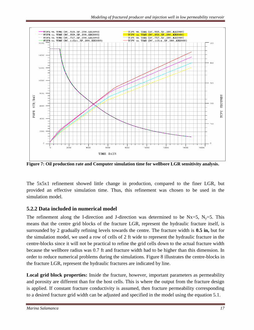
The graphic oil production rate and computer simulation time were the criteria of selection used to

evaluate the number of local grid refinement that should be used in the model simulation. The

optimal refinement will be one that presents small changes in production, compared to finer grid

blocks, as well as having significantly less simulation time. The results from the sensitivity

analysis are given in Figure 7.


Marina Salamanca 17

Figure 7: Oil production rate and Computer simulation time for wellbore LGR sensitivity analysis.

The 5x5x1 refinement showed little change in production, compared to the finer LGR, but

provided an effective simulation time. Thus, this refinement was chosen to be used in the

simulation model.

5.2.2 Data included in numerical model

The refinement along the I-direction and J-direction was determined to be Nx=5, Ny=5. This

means that the centre grid blocks of the fracture LGR, represent the hydraulic fracture itself, is

surrounded by 2 gradually refining levels towards the centre. The fracture width is 0.5 in, but for

the simulation model, we used a row of cells of 2 ft wide to represent the hydraulic fracture in the

centre-blocks since it will not be practical to refine the grid cells down to the actual fracture width

because the wellbore radius was 0.7 ft and fracture width had to be higher than this dimension. In

order to reduce numerical problems during the simulations. Figure 8 illustrates the centre-blocks in

the fracture LGR, represent the hydraulic fractures are indicated by line.

Local grid block properties: Inside the fracture, however, important parameters as permeability

and porosity are different than for the host cells. This is where the output from the fracture design

is applied. If constant fracture conductivity is assumed, then fracture permeability corresponding

to a desired fracture grid width can be adjusted and specified in the model using the equation 5.1.


Marina Salamanca 18

Where:

Equivalent fracture permeability

Equivalent fracture width

Figure 8: Fracture and wellbore LGR used in the model.

The value the input permeability for the hydraulic fracture has been scaled to preserve the actual

fracture width 0.5 in and the values the input such equivalent fracture permeability grid cell were

obtained from equation 5.1. Table 5 show the input values for the cells representing the hydraulic

fracture and the actual permeability of the hydraulic fracture.

Table 5: Input permeabilities for different fracture conductivities assuming the fracture width of 0.5

in

Fracture conductivity,

(0.5 in width)

mD *ft

Input fracture permeability

for 2 ft wide grid cells mD

Actual fracture permeability mD

1000 500 24000

2000 1000 48000

10000 5000 240000


Marina Salamanca 19

Figure 9 shows the results for vertical well fractured a coarse 5x5 LGR with 2 ft grid cell fracture

has been used. The result for this LGR is compared with 5x5 LGR real fracture width of 0.5 in. as

seen in figure 9 comparison shows very good agreement in oil production rate but in terms of

computational time the 5x5 with real fractures is taking more time and same problems during the

simulation.


for the fracture ( = 200 ft, conductivity of 2000 mD-ft).

For the LGR methods, the effects of changes in fracture length taking into account the global block

size is 400X400 ft the fracture half length ( ) has generally been run for 5 cases:

75 ft ( a partly fractured global cell)

200 ft (a fractured global cell)

300 ft (neighbour cell also partly fractured)

400 ft (neighbour cell also partly fractured)

600 ft (neighbour cell also fractured global cell)


Marina Salamanca 20

Figure 10: LGR of for a short vertical fracture of 75 ft half-length (global grid cell size is 400 ft).

Figure 10 presents the one global grid block defined with LGR blue lines where blue thick lines

are the effect of fine gridding. Fracture is extending in x direction with fracture half-length is 75,

defined by red line. Black circle in the center of the picture is the well.

Figure 11: LGR of for a vertical fracture of 400 ft half-length (global grid cell size is 400 ft).

Figure 11 presents the grid block defined with LGR. Blue lines where blue thick lines are the

effect of fine gridding. Fracture is extending in x direction with fracture half-length of 400, defined

by red line, for this the fracture extending in neighbor cell. Black circle in the center of the picture

is the well.


Marina Salamanca 21

5. 3 Verification of numerical model (Analytical solution)

To verify developed model, analytical solution for finite conductivity constant pressure for infinite

reservoir were used.

To be able to compare numerical simulation results to the analytical solution, it was necessary to

transform time and flow rate into dimensionless time in function of fracture half-length.

Correlation for dimensionless time in function of fracture half-length (Bennett et al.1986):

Correlations for dimensionless for flow rate are:

Where is the gamma function

Rock compressibility was calculated using equation (5.4) and based on numerical model data set:

Oil compressibility was calculated using equation (5.5) and based on numerical model data set:

Figure12. Presents graphical solution of numerical simulation (local grid refinement) results for

constant pressure case. The line red is for numerical simulation case and the line blue is for

analytical solution case. Match with analytical solution for a finite conductivity fracture provides

verification of numerical model for this case. The difference of approximately 2000 days is

because the blue line is for analytical solution to infinite reservoir or non-limited reservoir, then

the curve tends to infinite. While for red the line the simulator is limited reservoir then tends to

zero.


Marina Salamanca 22

Figure 12: Oil production total model simulation results with analytical solution for finite

conductivity type curve for constant pressure case.

5.4 Skin factor method

This method is easy to represent in simulation model because the value skin factor are gotten from

an analytical formula and after being put in model (in keyword COMPDAT).

Several skin values for the hydraulic fracture well were simulated to represent different fracture

lengths with the actual fracture width (0.5 in). However, the effective wellbore radius must be less

than the Peaceman’s radius (Cinco-Ley et al. 1978). This means that the fracture must stay within

the grid block in order to give a correct representation as a skin values.

Peaceman’s radius formulas

Pressure equivalent radius of the grid block is distance from the well at which the local pressure is

equal to the average nodal pressure of the block. Peaceman’s formula has been used in Cartesian

grid for rectangular grid blocks in an anisotropic reservoir:


Marina Salamanca 23

Where:

– the x and y dimensions of the grid block

x, and y directions permeabilities

Formulas below indicate the relationship between dimensionless fracture conductivity and the ratio

of effective wellbore radius to fracture half length (Cinco-Ley et al, 1987).However this formulas

was used to calculate in spreadsheet (as shown tables 6 and 7), and the final skin value were easily

entered in eclipse.

Table 6: values used for calculate the skin stimulation formulas

Table 7 shows the values of the skin factor obtained for different half lengths

Variable Description units

Reservoir permeability 10

Fracture permeability 48000

Fracture half-length 75

Fracture width (also referred as Wf) 0.042

power 1.1

constant 0.6 1

constant 0.515 1

wellbore radius 0.7


Marina Salamanca 24

Table 7: Input skin factor for different fracture conductivities

5.4.1 Skin factor vs LGR

The figure below shows a comparison of simulation results from skin factor and LGR for

representing hydraulic fracture in a vertical well. The hydraulic fracture conductivity was assumed

to be 2000 mD-ft and the hydraulic fracture lengths were 75, 200, 300, 400 and 600 ft.

The figure 13 shows that good agreement in terms of oil production rate and cumulative oil

production was given by the two methods in comparison when the fracture half-length (75 ft) is

located within the single grid area cell which contains the well.

Half length Values of Skin

75 -3.6

200 -4

300 -4.1

400 -4.2

600 -4.2


Marina Salamanca 25


line is for LGR method. The blue line is for skin factor method for a half-length 75 and hydraulic

fracture of 2000 mD-ft conductivities.


Marina Salamanca 26

Figure 14 shows the simulation results from local grid refinement and skin factor. Comparison of

the result shows very good agreement in oil production rate and cumulative oil production when

the fracture half-length (200 ft) is located within the single grid cell area which contains the well.



hydraulic fracture of 2000 mD-ft conductivities.


Marina Salamanca 27

Figure15 shows the simulation results from local grid refinement and skin factor methods.

Comparison of the result shows some discrepancy in oil production rate and cumulative oil

production when the hydraulic fracture (300 ft) is extended to neighbour grid cells. That means the

hydraulic fracture is not located within a single areal grid cell.





Marina Salamanca 28






line is for LGR method. The blue line is for skin factor method for a half-length is 400 and hydraulic

fracture of 2000 mD-ft conductivities.


Marina Salamanca 29






line is for skin factor method. The light blue line is for LGR method for a half-length is 600 and


The following conclusions can be made:

Comparison between local grid refinement and skin factor showed good agreement in oil

production when the vertical wellbore with hydraulic fractures are completely located

within a single areal grid cell.


Marina Salamanca 30

Comparison between local grid refinement and skin factor showed some discrepancy in oil

production when the vertical wellbore with hydraulic fractures extending to neighbours

grid cell.

The equivalent effective radius (skin factor) method provides more accurate results than

LGR because it is a simpler way to represent in a model. This method is applicable only if

the effective wellbore radius is smaller than the pressure equivalent radius of the grid cells.

In other words it requires that the vertical well with its hydraulics fractures should be

completely located within areal grid cell in order to get an accurate estimate of skin factor

to predict well productivity correctly.

5.5. Vertical well for heterogeneous reservoirs

The numerical modeling is similar to the previously described numerical modeling for vertical

wells in homogenous reservoirs.

Layer permeabilities

Layers 1-10; 21-30; 41-50; 61-70 2 mD

Layers 11-20; 31-40; 51-60; 71-80 20 mD

For the case of heterogeneous reservoir the skin factor for input model was simulated three ways

that were:

Average permeability of values ( AP)

In simulator model put of values of skin correspondent of two values of permeability

Average skin factor values (AS)


The figure below shows a comparison of simulation results from skin factor and LGR for

representing hydraulic fracture of a vertical well for heterogeneous reservoir. The hydraulic

fracture conductivity was assumed to be 2000 md-ft and the hydraulic fracture lengths were 75,

200, 300, 400 and 600 ft.


Marina Salamanca 31

The figure 18 shows the simulation results from local grid refinement and skin factor. Comparison

of the result shows very good agreement in oil production rate when the fracture half-length (75 ft)

is located within the single grid cell area which contains the well.


heterogeneous reservoir for a half-length is 75 and hydraulic fracture of 2000 mD-ft conductivities.


Marina Salamanca 32

Figure 19 shows the simulation results from local grid refinement and skin factor. Comparison of

the results shows very good agreement in oil production rate when the fracture half-length (200 ft)

is located within the single grid cell area which contains the well.




Marina Salamanca 33

Figure 20 shows the simulation results from local grid refinement and skin factor methods.

Comparison of the results shows some difference in oil production rate when the hydraulic fracture

(300 ft) is extended to neighbour grid cells. That means the hydraulic fracture is not located within

a single areal grid cell.




Marina Salamanca 34


Comparison of the results shows some difference in oil production rate when the hydraulic fracture






Marina Salamanca 35


Comparison of the result shows some difference in oil production rate when the hydraulic fracture





The following conclusions are collected from the analysis:

Comparison between local grid refinement and skin factor methods to heterogeneous

reservoir showed good agreements in oil production when the vertical wellbore with

hydraulic fractures are completely located within a single areal grid cell.

Comparison between local grid refinement and skin factor methods to heterogeneous

reservoir showed some discrepancy in oil production when the vertical wellbore with

hydraulic fractures extends to neighbours grid cell.


Marina Salamanca 36

The equivalent wellbore radius method, compared to the LGR is more flexible regarding

large scale simulations. However this method has one limitation, the effective wellbore

radius must be smaller than the pressure equivalent radius. In other words the fractured

vertical wellbore must be located within one single areal grid blocks.

5.6 Conductive fractures (Eclipse 300)

To generate this method in reservoir simulator the paths of fracture planar segments were specified

through the grid blocks, the effective aperture, fractures permeability and saturation table.

Fracture width 0.5 in was very low and unacceptable for simulation by simulator because the well

bore radius was 0.7 ft and fracture width had to be higher than this dimension. The most

convenient dimension was 2 ft, the dimension of the smallest grid block with well.

The fracture direction is specifies in COMPDAT keyword. The well intersection behavior is

controlled using the WELLCF keyword.

The fracture half-lengths ranged from 200 ft and 600 ft the global block size is 400X400 ft. As

shows the figure 23 and 24

- 200 ft (a fractured global cell)

- 600 ft (neighbors cell also global cell)

Figure 23: conductivity fractures for vertical fracture of 200 ft half-length (global grid cell size is 400

ft).


Marina Salamanca 37

Figure 24: Conductivity fractures for vertical fracture of 600 ft half-length (global grid cell size is 400

ft).

Figure 25 shows the simulation results from Eclipse 100 and 300 without fractures. Comparison of

the results shows very good agreement in oil production when we used eclipse 100 and 300.

Figure 25: Comparison of results of the base case from Eclipse 100 and 300 without fractures


Marina Salamanca 38

5.6.1 LGR vs Conductive fractures (Eclipse 300)

Figure 26 and 27 compares oil production rate and oil production total performance from

simulation cases using conductive fractures (Eclipse 300) and LGR methods.

The hydraulic fracture was assumed to be 2000 mD-ft and the hydraulic fracture lengths were 200

ft and 600 ft. The results shows that the conductivity fracture method can greatly under-predict oil

production in comparison with the LGR method.

The figure 26 shows that some discrepancy in terms of oil production rate and cumulative oil

production was given by the two methods in comparison when the fracture half-length (200 ft) is

located within the single grid cell area which contains the well.

Figure 26: Comparison of results from conductivity fractures method with those from LGR method.

The green line is for conductive fractures method the light blue line is for LGR method for a half-

length is 200 and hydraulic fracture of 2000 mD-ft conductivities.


Marina Salamanca 39

The figure 27 shows that good agreement in terms of oil production rate and cumulative oil

production was given by the two methods in comparison when the fracture half-length (600 ft)

extended to neighbour grid cells. That means the hydraulic fracture is not located within a single

areal grid cell.

Figure 27: Comparison of results from conductivity fractures method with those from LGR method.

The green line is for conductive fractures method the light blue line is for LGR method for a half-

length is 600 and hydraulic fracture of 2000 mD-ft conductivities.

The following conclusions are collected from the analysis:

Comparison between local grid refinement and conductivity fractures (Eclipse 300)

showed good agreement in oil production when the hydraulic fracture extend over areal

grid cell. We can say this method is good when we get longer fractures.

The local grid refinement method provides more accurate results than the conductivity

fracture method because geometry of the fractures are modeled and represented by very

fine grid blocks. Properties of the fractures, such as permeability, are assigned to those


Marina Salamanca 40

fracture blocks. With the conductivity fractures method the grid block properties that

contain the fracture are modified during the simulation. Thus, this can significantly affect

the accuracy.

5.7 Sensivity analyses

The simulation model developed was applied in different scenarios. Scenario 1 was a base case

study for a non-fractured setting. In order to understand the effects of hydraulic fracturing,

Scenario 2 with fractures were evaluated for effect of fracture half length, conductivity fracture

and effect rock permeability. In Scenario 3 the analysis was evaluating number of fractures in

horizontal wells.

5.7.1 Scenario 1: Non-fractured wells

A base case scenario, where none of the wells were fractured was simulated in this scenario, and

then compared with wells which contain hydraulics fracturing, each one having constant formation

permeability. The main objective of this scenario is to analyze the increase in production of a well

fractured with vertical fracture in relation to non- fractured wells.

Figures 28 and 29 shows the results of oil production rates on the primary y-axis and the oil

production total on the secondary y-axis for non-fractured well and fractured well respectively.

The result shows clearly that hydraulics fracturing improves the oil production rate. Due to the

increase the permeability near of wellbore, the connectivity between wells and reservoir improves.

Thus, the fluid flow efficiency improves as well.


Marina Salamanca 41

Figure 28: Oil production rate from a vertical well for local grid refinement methods values. For base

case without fractures is green line of the light blue is with fractures.


Marina Salamanca 42

Figure 29: Oil production rate from a vertical well of different skin values. The green line denotes the

case of skin 0, the blue line is for the case skin of -4.

The conclusion from this case is that the reservoir has potential for increase in productivity by

connectivity enhancement, by, for instance, hydraulic fracturing.

5.7.2 Scenario 2: fractured wells

Effect of fracture conductivity

In this scenario sensitivity analysis were performed on the impact of the fracture conductivity,

during this step changes were made in model. The performance of the simulations under different

conductivity, 1000, 2000 and 10000 has been simulated. The objective was to get an optimized

estimate of the oil production.

Figure 30 shows the results of oil production rates on the primary y-axis and the oil production

total on the secondary y-axis for different conductivity fractures 1000, 2000 and 10000 with half-

length 200 ft for local grid refinement methods. The result shows clearly that increasing fracture

conductivity (proppant) leads to increase in oil production rate.


Marina Salamanca 43

From equation 2.2 and figures 30 we can see for fixed half-length and fixed reservoir permeability,

that the fracture conductivity increase and the value increase. The focus is then on maximizing

the fracture permeability and width. This is done by choosing appropriate materials and treatment

procedures.

Figure 30: Oil production rate from a vertical well of different fracture conductivity values. The light

blue line denotes the case of 10000 conductivity fractures. The blue line is for the case of conductivity

fractures of 2000. The green line is the case for conductivity fractures of 1000.

Effect of rock permeability

For study of rock permeability, in addition to the Base Case rock permeability (K=10 mD), three

permeabilities K=0.1 mD, k =1mD and K=100mD have been simulated. The objective is to studies

how the rock permeability can affect hydraulics fracture.

Figure 31 shows the results of simulations oil production rate for different permeabilities 0.1,1,10

and 100 for conductivity fracture 2000 md-ft in half-length 200 ft for local grid refinement

methods. The results clearly indicate increased permeability the oil production increase. This means

higher permeability reservoir. It is very difficult to get significant enhancement using hydraulic


Marina Salamanca 44

fracturing. In other words the conductivity fracturing is typically used only in low permeability

reservoir.

Figure 31: Oil production rate from a vertical well of different rock permeabilities. For the case of

fracture conductivity of 2000 and half-length of 200 ft.

The conclusion from this case is that the production in the reservoir is sensitive to changes in formation

permeability.

Effect of half length

Several values have been chosen for this investigation for fracture half lengths variations in

simulation model. Were analyzed 5 cases taking into account the following fracture lengths 75,

200, 300, 400 and 600 ft.

The figure 32 and 33 shows of simulations oil production rate for different half lengths, the

hydraulic fracture conductivity was assumed to be 2000 mD-ft and the hydraulic fracture lengths

were 75, 200, 300, 400 and 600 ft for local grid regiment method is the case for skin factor

methods. From the figures we can see that the optimal situation in most likely the case with 300


Marina Salamanca 45

half-length stimulations because there is almost no incremental production from the 400 and 600

half length.

From the equation 2.2 and figures 32 and 33 we can say that for fixed proppant type and fixed

reservoir permeability, as the fracture half-length increase, value decreases. Thus, an increase

in the fracture length will not necessarily yield a significant gain in effective radius and therefore

no significant gain in well productivity. In other words long fractures would give higher

productivity than short fractures. Nevertheless, the incremental gain in productivity diminishes as

finite conductivity fracture becomes longer. This is because the pressure drops within the fractures

itself, which may be comparable to the reservoir pressure drop resulting in a diminishing

incremental gain in the productivity with length.

Figure 32: Oil production rate from a vertical well of different half lengths values. For local grid

refinement methods.


Marina Salamanca 46

Figure 33: Oil production rate from a vertical well of different half lengths values. For skin factor

methods


Marina Salamanca 47

6. Numerical modeling of horizontal well

6.1. Numerical Modeling Methodology

Numerical modeling of horizontal is similar to the previously described numerical modeling of

homogenous vertical wells. The same model with synthetic data of reservoir, and fracture

geometry and fluid properties.

A 2400 ft long horizontal well was placed in the layer 40 of the model as shown in figure 33.

Three transverse fractures from base to top of the grid were created and modeled with fracture

half-length 200 ft. Red in the center of the picture is the well.

Figure 34: Locations of the transverse hydraulic fractures of the horizontal well modeled by using

LGR. For a transverse fracture of 200 ft half-length.

Where equivalent fracture width must be higher than the well bore radius and in this case it was

convenient to set it to 2 ft because that was dimension of the grid block with well.

Calculated real and equivalent fracture permeability using correlation (5.1)

The figure 35 shows the results compared to horizontal well fractured well with a coarse 5x5 LGR

2 ft grid cell fracture has been used and with 5x5 LGR real fracture width of 0.5 in. The result

shows very good agreement with oil production rate.

Fracture LGR 5X5


Marina Salamanca 48


for horizontal well with fracture ( = 200 ft, conductivity of 2000 mD-ft).


The fractured horizontal well is modeled as a standard vertical well using Peaceman’s formula and

an equivalent wellbore radius. This means the equivalent wellbore radius concept is applicable

only if the effective wellbore radius is smaller than pressure equivalent radius. This restriction

requires that the horizontal wellbore with hydraulic fractures are completely within a single areal

grid cell.

Peaceman’s radius formulas

For reservoir isotropic the pressure wellbore radius is:

Horizontal well

Figure 36 compares simulated oil production rate and oil production total from the case where the

three hydraulic fractures were modeled using a skin factor of -3 for all the connections and the

case where the LGR method was used to model these fractures (half-length of 200 ft). It clearly

shows that oil production is significantly poor when skin factor method was used. This is due to

the effective wellbore radius is higher than the pressure equivalent radius because the grid block


Marina Salamanca 49

size in direction Z is very small (approximately 4 Thus in this case the equivalent wellbore

radius method cannot be applicable.

Figure 36: Comparison of oil production from cases when the hydraulic fractures are modeled using

skin factor and using LGR. The lines in green are for the skin of -3 case; the lines in blue is for the

LGR case.

The conclusion from this case is that for horizontal wells the methods of equivalent wellbore radius

is not applicable for this case. Due to the fractured horizontal well is not located within one single

areal grid blocks.


Marina Salamanca 50

6.1.2 LGR vs Conductive fractures (Eclipse 300)

Figure 37 compares simulated oil production rate and oil production total from the case where the

three hydraulic fractures were modeled using conductivity fracture (Eclipse 300) and the case

where the LGR method was used to model these fractures (half-length of 200 ft). It clearly shows

that oil production is poor when conductive fractures (Eclipse 300) method was used. Because the

Eclipse is not cleary when this method is tested for horizontal well. For horizontal well this

methods was not tested (Van Lingen et al. 2001).

Figure 37: Comparison of oil production from cases when the hydraulic fractures are modeled using

conductivity fracture methods and LGR methods. The lines in green are for the conductive fracture

and the line in blue is for the LGR case.

The conclusion from this case is that for horizontal wells the methods of conductive fractures is not

applicable for this case.


Marina Salamanca 51

6.1.3 Scenario 3: Number fractured wells

In this scenario the effect of number fractures in horizontal well was studied. Three runs were

simulated, to 1, 2, and 3 fractures having a constant formation permeability of 10 mD. The

objective was to understand how number of hydraulic fractures can influence the recovery factor.

Figure 38 shows simulated well oil production from the case where we have 1, 2 and 3 transverse

hydraulic fractures. These transverse hydraulic fractures were modeled using LGR. We can see

that the optimal situation is most likely the case with three fracture stimulations.

Figure 38: Comparison of oil production for one to three longitudinal fractures in horizontal well for

the case conductivity fracture 2000 mD-ft and half-length 200 ft.


Marina Salamanca 52

7. Thermal fractures

Modeling of thermally induced fracturing involves an estimation of fracture width, height and

length as functions of in-situ stress, injection rate and temperature, and rock and fluid properties.

7.1 Modeling fracture growth in injection well

We present a model of the initiation and growth of a fracture in the near wellbore. In this case we

used two vertical wells, an injector and a producer respectively. The first both vertical well is

producer but after 4 years it becomes injector (0P02). The injection well with a constant flow of

water 10000 STB/day is restricted to operate at a maximum pressure of 20000 psi and is

completed in the lower layer. The production well (0P01) is completed in the upper and operates at

a constant minimum background pressure of 8000 psi. The simulation was proposed for 3653 days

using a fully implicit solution scheme for both the mother and for the fracture system the software

used is reveal.

Table 8: Summary of input parameters for the single well simulations.

Fluid injection Properties

The stress will be calculated as functions of following parameters are: In-Situ Stress, temperature,

pressure, Poisson’s ratio, young’s modulus.

When the fluids injected into formation are cooler than formation. This causes a region of cooled

rock to develop around the injection well. This change in temperature causes the rock contract or

expands, thereby to decrease in horizontal earth stresses around the injection well. The reduction

in horizontal stresses causes hydraulics fractures pressure for the rock. Thus the presence of a two-

winged vertical fracture the flood front would be elliptical during injection (as shown in Figure

39.).

Permeability 10 md

Porosity 0.2

Initial reservoir temperature 200 OF

Min. horizontal stress 6000 psi

Young’s Modulus 13000 Pa

Poisson’s Ratio 0.25

Poro-elastic coefficient 0.3

Thermo-elastic coefficient 20

Injection Water Temperature 77 oF

Injection Rate 10000 STB/ day


Marina Salamanca 53

Figure 39: Plan view of a growing two-winged fracture in simulator

An important factor to be considered here is that injection well is not fractured at the

commencement of injection. Fracturing is induced during the course of injection and these

fractures grow with time.

The basic principle of thermal fracture model is:

Flow, pressure, temperature supplied by an injection

Rock mechanics of fracture

7.1.2 Effect of particle plugging

The concetrantion of injected particles has an effect in initation and propagation of fractures.

When the fluids containing suspended particles are injected into a fracture, the particles invade the

formation adjacent to the fracture face and reduce the permeability in the near wellbore region.

Hence an increased bottom hole injection is required to maintain a given injection rate. When the

fracture is exceeded fractures are initiated. Further when the pressure at the tip exceeds the

propagation pressure, the fractures propagates. Injection well fracture grows very slowly as shown

in Figure 39.

Results from run fig 40 shows larger particle concentration lead larger values of injection due to

increase in pressure which contributes to larger fracture lenghts.

Injection of particle at increasingly larger concentration will increase the rate of buidup of internal

and external filter cakes due to an increasingly larges volume of particles being deposited.

The internal and external cake resistences decrease during fracture propagation directly to the area

of the fracture face when the fracture face is relatively small, high injected particles concentration


Marina Salamanca 54

result in large value of pressure which maintain large fracture half lenghts as shown in Figure 40

The higher the particle concentration, the faster the formation is plugged. Hence the fracture is

initiated earlier. Also, fractures propagate faster due to faster plugging of the fracture face. The

shape (ladder) of curves were caused due to the values of the time used for the simulations

Figure 40: Effect of injected particle concentration on fracture growth with time.


Marina Salamanca 55

Results from figure 41 indicate that as water breakthrough delays as concentration increases. And

it also indicates the greater the concentration the smaller the water cut.

Figure 41: Effect of injected particle concentration on water cut.


Marina Salamanca 56

Results from the figure 42 illustrate that oil production increases as concentration increases. For

the case equal 25 ppm provided the longest fracture half length, but this fracture did not reach the

producer instead improved the water sweep efficiency.

Figure 42: Effect of injected particle concentration on oil produced.

The conclusion from this case is that creation of fractures in injector due to particles plugging can

accelerate oil production but also lead to delay water breakthrough in water flooding applications.


Marina Salamanca 57

7.1.3 Effect of flow rate

Fig. 43 shows that simulations the injection of flow rate significantly increase the fracture growth

rate. High injection rates resulted in earlier formation fracturing because large bottom hole

pressures are required to inject at high rates. The shape (ladder) of curves was caused due to the

values of the time used for the simulations. The last part of the green line (rate =15000 STB/day)

was caused by numerical error.

Figure 43: Effect of flow rate on fracture length.


Marina Salamanca 58

Simulation results shown in Figure 44 indicate that low injection rates provided late water

breakthrough and high cumulative oil produced. Due to bottom hole pressure associated with

injection.

Figure 44: Effect of flow rate on water cut


Marina Salamanca 59

Simulation results shown in Figure 45 indicate that high rate the oil produced increase this is

because as the fracture length increases, the areas previously un-swept are better swept. Hence the

oil recovery increases with increasing rate of fracture growth.

Figure 45: Effect of flow rate on oil produced

The conclusion from this case is that creation of fractures in injector can accelerate oil production

but also lead to early water breakthrough in water flooding.


Marina Salamanca 60

The figure 46 compares oil production rate performance from simulation cases using Eclipse and

Reveal software. The results show good agreement between software.

.

Figure 46: Comparison oil production rate performance from simulation cases using Eclipse and

Reveal software


Marina Salamanca 61

8. Summary and Recommendations

8.1. Summary

The method of fractured well representation with skin factor set up is one of the simplest.

The main problem with this method is the indifference to fracture direction and

underestimates vertical flow horizontal.

The local grid refinement method in simulator model can be locally refined (near the

wellbore) and permeability of some of them can be modified. The main advantage of this

method is accuracy. The direction of the fracture propagation can be taken into account,

grid blocks directions coincides with fracture direction and near wellbore geometry is

realistically presented. The main problem of this methods is only two direction can be

modeled, complicated to set up and the high computational time.

The conductivity fracture method in simulator model increase inflow of the relatively high

permeability fracture. The main problem associated with this method is the grid block

properties are modified to take account of the physical void introduced by the fractures.

Thus, is not expected gives good results for short fractures

For vertical wells with vertical fractures, skin factor method seems the first choice to

represent the hydraulic fractures in the simulation model because it simpler model

fractured vertical well in field models. This method is applicable only if the effective

wellbore radius is smaller than the pressure equivalent radius of the grid cells, and efficient

in CPU time.

Local grid refinement method can represent the hydraulic fractures more accurately and

thus gives the best accuracy for both fractured vertical and horizontal wells.

For horizontal wells with transverse hydraulic fractures the skin factor and conductivity

fracture method have a poor accuracy and should not be used.

A model for fracture growth in vertical injector has been developed. It is clearly shows that

the rate of fracture growth depends on the injection rate, water quality, temperature as well

as the mechanical properties of the rock. The injectivity is primarily dependent on the in-

situ stresses, injection rate and the water quality.

Growing injection well fractures can have a significant impact on the sweep and oil

recovery.


Marina Salamanca 62

8.2. Recommendations for Future Work

The future work includes the application of the analytical solution for horizontal wells.

Simulation with simplified fracture growth behavior in eclipse to reproduce Reveal

simulation results.


Marina Salamanca 63

References

Agarwal, R.G., Carter, R.D., Polloc, C.B., – Evaluation and Performance Prediction of Low-

Permeability Gas Wells Stimulated by Massive Hydraulic Fracturing –Journal of Petroleum

Technology, March 1979, 362-372, Trans. AIME 267.

Ali Ghalambor, Syed A. Ali, W. David Norman.; Frac Packing Handbook, 2009

A. Settari, SPE “Simulation of Hydraulic Fracturing Processes” Intercomp Resource

Development and Engineering Inc.

Bennett, C.O., Reynolds, A.C., Raghavan,R., Jacques, L.E., – Performance of Finite Conductivity,

Vertically Fractured Wells in Single-Layer Reservoirs – SPE Formation Evaluation – August 1986,

399-412

Brown, J.E.; Economides, M.J.; “An Analysis of Hydraulically Fractured Horizontal Wells”, SPE

24322, 1992.

B.R Meyer, SPE and R.H. Jacot, SPE, Meyer & Assocs.; “Pseudosteady-States Analysis of Finite-

Conductivity Vertical Fractures”, SPE 95941, 2005.

Section 5. Basic Well Test Interpretation. Introduction to Well Testing (March 1998). 5-2.

Schlumberger.

Cinco-Ley, H., Samaniego, V.F., Dominguez, N.,– Transient Pressure Behavior for a Well With

Finite-Conductivity Fracture – SPE Journal, August 1978, 253-264, Trans. AIME 265.

Cinco-Ley, H., Ramey, Jr., H.J., Samaniego, F., Rodriguez, F.: "Behaviour of Wells with Low-

Conductivity Vertical Fractures," paper SPE 16766, presented at the SPE 62nd Annual Technical

Conference and Exhibition, Dallas, Texas, Sept. 27-30, 1987

Cinco-Ley, H., Samaniego, V.F., – Transient Pressure Analysis for Fractured Wells – SPE paper 7490,

Journal of Petroleum Technology, September 1981, 1749-1766

Clark, J.B.; “A Hydraulic Process for Increasing the Productivity of Wells”, 1949, SPE 949001

Ding, Y.; “Modelling of Fractured Wells in Reservoir Simulation”, SPE 36668, 1996

D.G. Crosby, M.M. Rahman, M.K. Rahman, S.S. Rahman“Single and multiple transverse fracture

initiation from horizontal wells” Journal of Petroleum Science and Engineering 35 (2002) 191–

204, 2001

Ehrl, E., Schueler, S.K.; “Simulation of a Tight Gas Reservoir with Horizontal Multifractured

Wells”, SPE 65108, 2000

ECLIPSE manual

Economides, M.J., Nolte, K.G.; “Reservoir Stimulation, Third Edition”, Wiley, England, 2000.


Marina Salamanca 64

Fjær, E., Holt, R.M, Horsrud, P., Raaen, A.M., Risnes, R.; “Petroleum Related Rock Mechanics –

2nd Edition”, Elsvier, Netherland, 2008

H. Mahdiyar, M.Jamiolahmady, and A. Danesh, Herriot-Watt U. “ New Mechaminal and damage

Skin factor Correlations for Hydraulically fractured” SPE 107634 2007

Hegre, T.M.; “Hydraulically Fractured Horizontal Well Simulation”, SPE 35506, 1996

Larsen, L., Hegre, T.M.; “Pressure Transient Analysis of Multifractured Horizontal Wells”,

SPE 28389, 1994.

Lake, L.W., Clegg, J.D.; “Petroleum Engineering Handbook Volume 4: Production Operations

Engineering, Chapter 8: “Hydraulic Fracturing”, Holditch, S.A., SPE, 2007.

Nashawi, I.S, Malallah, A.H – Well Test Analysis of Finite-Conductivity Fractured Wells Producing at

Constant Bottomhole Pressure – Journal of Petroleum Science and Engineering – 57 (2007), 303-320.

Nigel G. Higgs.; “ Injection Fracture Pressure Predictions for Vito Field, Deepwater Gulf of

Mexico”, 2011

Peaceman, D.W.; “Interpretation of Well-Block Pressures in Numerical Reservoir Simulation

with Non-Square Grid Blocks and Anisotropic Permeability”, SPE 10528, 1983.

Perkins, T. K. and J. A. Gonzalez, “The effect of thermoelastic stresses on injection well

fracturing”, SPE Journal, 25(1):78-88, February 1985.

Paul van Lingen (Institut Français du Pétrole), Mustafa Sengul (Saudi Aramco), Jean-Marc Daniel

(Institut Français du Pétrole), Luca Cosentino (Beicip-Franlab).; “Single Medium Simulation of

Reservoirs with Conductive Faults and Fractures”, SPE 68165 2001,

Phani B. Gadde, SPE, and Mukul M. Sharma SPE, University of Texas at Austin “Growing

Injection Well Fractures and Their Impact on Waterflood Performance” SPE 71614, 2001.

Rajagopal Raghavan, Curtis O. Bennett, Albert C. Reynoldes Jacques L. Elibel “ Perfomace of

Finite-Conductivity, Vertically fractured wells in single layer reservoirs. SPE 11029

REVEAL manual.

Soleimani, A., Lee, B., Ghuwaidi, Y., Dyer, S.; “Numerical Modelling of Multiple Hydraulically

Fractured Horizontal Wells”, SPE 120552, 2009.

Soliman, M.Y., Hunt, J.L., El Rabaa, A.M.; “Fracturing Aspects of Horizontal Wells”, SPE 18542,

1990.

T.M. Hegre, Petec A/S, and Lelf Larsen, Statoil A/S “Productivity of Multifractured Horizontal

Wells”, SPE 28845, 1994.

Wan, J., Aziz, K.; “Semi-Analytical Well Model of Horizontal Wells With Multiple Hydraulic

Fractures”, SPE 81190, 2002.


Marina Salamanca 65

Valkó, P., Economides, M.J.; “Hydraulic Fracture Mechanics”, Wiley, England, 1995. . http://www.petrocenter.com/reservoir/prod%20index.htm

Y. Abacioglu, Sebastian, H.M., Oluwa, J.B.; “Advancing Reservoir Simulation Capabilities for

Tight Gas Reservoirs”, SPE 122793, 2009.

http://www.petrocenter.com/reservoir/prod%20index.htm


Marina Salamanca 66

Nomenclature

Fracture permeability [mD]

Formation permeability [mD]

Conductivity fracture [mD-ft]

Dimensionless fracture conductivity

Fracture within [ft]

porosity

fracture porosity

viscosity

dimensionless pressure

Initial pressure

Bottom hole flowing pressure

fluid FVF [STB/day]

Flow rate

dimensionless flow rate

pressure equivalent radius of the grid block [ft]

Wellbore radius [ft]

Fracture half- length [ft]

Formation permeability in direction [mD]

Formation permeability in direction [mD]

Formation height [ft]

Dimensions of the grid block direction

Dimensions of the grid block direction

Production time [days]

Dimensionless time in function of the fracture half-length

Rock surface energy


Marina Salamanca 67

Young’s modulos

Radius of extending edge of the fracture

Poisson’s ratio

Abbrevations

Local grid refinement

Productivity index

Bottom hole pressure

Field oil production rate

Field oil production total


Marina Salamanca 68

Appendix A Simulation cases

The Eclipse reservoir simulation cases for the Comparative Study on Methods of Simulating

Hydraulically Fractured Wells are located on project area:

A.1 Example on Eclipse LGR set-up for a vertical well

-- WELL SEGMENT SIMULATION MODEL (2013) -

-- Marina Salamanca Master Thesis

-- ZONE 1 K: 1 - 30

-- ZONE 2 K: 31 - 80

-- ZONE 3 K: 81 -130

-- ZONE 4 K:130 -170

--

====================================================================================

======

RUNSPEC

--

====================================================================================

======

--

TITLE

WELL SECTOR MODEL

--

START

1 'JAN' 2020 /

--

DIMENS

-- NX NY NZ

19 36 170 / 116,280 cells; Areal resolution approx 400m x 400m

--

OIL

WATER

GAS

DISGAS

VAPOIL

--

-- Unit system

FIELD

--

MEMORY

3000 /

--

TABDIMS

-- NTSFUN NTPVT NSSFUN NPPVT NTFIP NRPVT

1 1 22 100 4 20 /

--

EQLDIMS

-- NTEQUL

1 /

--

REGDIMS -- Added to run MULTNUM for region transmissibility multipliers

6 1 /

--

GRIDOPTS -- Added to run MULTNUM for region transmissibility multipliers


Marina Salamanca 69

YES 6 0 /

--

FAULTDIM

-- MFSEGS: maximum number of fault segments

100000 /

-- Well dimension data (10 items)

WELLDIMS

-- MNWELL MNCONN MNGRPS MNWIGRP

1 500 2 20 /

-- Production wells VFP table dimensions (6 items)

VFPPDIMS

--FVPTMX THPPTMX WCTPTMX GORPTMX ALQPT VFPTMX

20 10 10 5 1 1 /

-- Injection wells VFP table dimensions (3 items)

--VFPIDIMS

--FVPTMX THPPTMX VFPTMX

10 10 10 /

--Allow for endpoint scaling

ENDSCALE

/

--

-- Reset message print and stop limits

MESSAGES

-- Severity

-- 1 2 3 4 5 6

-- Messages Comment Warning Problem Error Bug , Stop values follow

1000000 1000000 10000 10000 10000 10000 1000000 1000000 100000 10000 /

--

---- Request output of SAVE file for fast restart

--SAVE

--/

--

-- Linear solver stack size (size of search directions held by the ORTHOMIN linear solver)

-- Default is 10. There is no point in setting NSTACK larger than LITMAX (See TUNING)

--

NSTACK

100 /

--

-- Input files are unified

UNIFIN

--

UNIFOUT

--

ROCKCOMP

IRREVERS 1 NO/

--

--NOSIM

--

====================================================================================

======

GRID


Marina Salamanca 70

--

====================================================================================

======

-------- IN THIS SECTION , THE GEOMETRY OF THE SIMULATION GRID AND THE

-------- ROCK PERMEABILITIES AND POROSITIES ARE DEFINED.

------------------------------------------------------------------------

--

INIT

--

NEWTRAN

--

NOECHO

--

INCLUDE

'../include/ecl_grid.grdecl' /

--

INCLUDE

'../include/ecl_grid.faults.grdecl' /

--

INCLUDE

'../include/ecl_grid.permx.inc' /

--

INCLUDE

'../include/ecl_grid.poro.inc' /

--

EQUALS

-- I1 I2 J1 J2 K1 K2

PERMX 10 1 19 1 36 1 170 /

PORO 0.20 1 19 1 36 1 170 /

ACTNUM 0 1 19 1 36 81 170 /

/

-- Populate PERMY=PERMX and PERMZ=fraction of PERMX

COPY

'PERMX' 'PERMY' /

'PERMX' 'PERMZ' /

/

MULTIPLY

'PERMZ' 0.01 /

/

--Faults are assumed Closed as a base case

MULTFLT

-- NAME MULTIPLIER

'smcl_02' 0.01 /

'smcl_04' 0.01 /

'smcl_05' 0.01 /

'smcl_06' 0.01 /

/

CARFIN

'0P01BLK' 15 15 29 29 1 170 5 5 170 1 /

HXFIN

125 3*50 125 /

HYFIN


Marina Salamanca 71

139 60 2 60 139 /

NZFIN

170*1 /

EQUALS

--Name Value

PERMX 1000 1 5 3 3 1 170 /

PERMY 1000 /

PERMZ 1000. /

PORO 0.30 /

/

-- Re-enable echoing of the input file (to the PRT file)

NOECHO

--

--

====================================================================================

======

EDIT

--

====================================================================================

======

PROPS

-------- THE PROPS SECTION DEFINES THE REL. PERMEABILITIES, CAPILLARY

-------- PRESSURES, AND THE PVT PROPERTIES OF THE RESERVOIR FLUIDS

--

====================================================================================

======

NOECHO

--

--RSCONST

-- 0.4014 1500 /

--

SCALECRS

NO /

--

INCLUDE

'../include/ecl_grid.swl.inc' / -- This keyword specify the connate water saturation

--

EQUALS

-- I1 I2 J1 J2 K1 K2

SWL 0.30 1 19 1 36 1 170 /

/

COPY

'SWL' 'SWCR' /

'SWL' 'SGU' /

/

--

MAXVALUE

SWL 0.65 /

SWCR 0.65 / --The SWCR and ISWCR keywords specify the critical water saturation

/

EQUALS


Marina Salamanca 72

-- I1 I2 J1 J2 K1 K2

SOWCR 0.0001 1 19 1 36 1 170 /

/

--

EQUALS

SWU 1.00 / --This keyword specify the maximum water saturation

/

MULTIPLY

'SGU' -1 /

/

ADD

'SGU' 1 /

/

--

SWOF

--

-- Swi = 0.35 & Sorw = 0.32 no = 3, nw = 1.5

-- Sw krw krow Pc

0.3500 0.0000 1.0000 0

0.3685 0.0021 0.8887 0

0.3870 0.0071 0.7848 0

0.4055 0.0145 0.6881 0

0.4240 0.0239 0.5986 0

0.4425 0.0354 0.5160 0

0.4610 0.0486 0.4403 0

0.4795 0.0637 0.3713 0

0.4980 0.0805 0.3089 0

0.5165 0.0989 0.2528 0

0.5350 0.1189 0.2031 0

0.5535 0.1405 0.1594 0

0.5720 0.1636 0.1215 0

0.5905 0.1882 0.0894 0

0.6090 0.2143 0.0627 0

0.6275 0.2418 0.0412 0

0.6460 0.2707 0.0247 0

0.6645 0.3010 0.0127 0

0.6830 0.3326 0.0050 0

0.7015 0.3657 0.0010 0

0.7200 0.3990 0.0000 0

1.0000 1.0000 0.0000 0

/

--

SGOF

-- dummy - no free gas

0.00 0 1 0

0.65 1 0 0

/

INCLUDE

'../include/BC_UPDATED-PVT_IX_SOL.INC' /

ROCKTAB

--Pressure PORVmult Transmissibility-mult

10397 0.965 0.70

11847 0.970 0.73

13297 0.974 0.77


Marina Salamanca 73

14747 0.978 0.81

16197 0.983 0.85

17647 0.987 0.89

19097 0.991 0.92

20547 0.996 0.96

21997 1.000 1.00 /

--

====================================================================================

======

REGIONS

--

====================================================================================

======

NOECHO

--

EQUALS

-- I1 I2 J1 J2 K1 K2

EQLNUM 1 1 19 1 36 1 170 /

SATNUM 1 1 19 1 36 1 170 /

PVTNUM 1 1 19 1 36 1 170 /

FIPNUM 1 1 19 1 36 1 30 /

FIPNUM 2 1 19 1 36 31 80 /

FIPNUM 3 1 19 1 36 81 130 /

FIPNUM 4 1 19 1 36 131 170 /

/

ECHO

--

====================================================================================

======

SOLUTION

--

====================================================================================

======

--

-- Datum depth at 29500 m TVD SS

-- DATUM DATUM OWC OWC GOC GOC RSVD RVVD SOLN

-- DEPTH PRESS DEPTH PCOW DEPTH PCOG TABLE TABLE METHOD

EQUIL

25626 19410 26220 0 19410 0 1 1 0 / -- OWC

RSVD

19410 0.4014

40000 0.4014

/

RVVD

10000 0.0097116

19410 0.0097116

/

--

RPTSOL

'RESTART=2' 'FIP=3' 'PRES' 'SOIL' 'SWAT' 'SGAS' 'RECOV' /

--

RPTRST


Marina Salamanca 74

'BASIC=5' 'FIP' 'POT' /

--

--

====================================================================================

======

SUMMARY

--

====================================================================================

======

--

INCLUDE

'../include/summary.inc' /

--

--

====================================================================================

======

SCHEDULE

--

====================================================================================

======

NOECHO

-- Hydraulic tables with 4" tubing (no ESP).

INCLUDE

'../include/VLP_4INCH.inc' /

--

RPTSCHED

'FIP=3' 'SUMMARY=2' 'CPU=3' 'RECOV' /

--

RPTRST

BASIC=4 FREQ=2 /

--

NOECHO

--

GRUPTREE

'G' 'FIELD' /

/

TUNING

1 14 0.1 /

/

/

/

--

WELSPECL

'0P01' 'PROD' '0P01BLK' 3 3 1* 'OIL' /

/

COMPDATL......................................................

'0P01' '0P01BLK' 3 3 1 170 'OPEN' 2* 1* 1* /

/

/

WCONPROD

'0P01' 'OPEN' 'BHP' * 1* 30000 1* 1* 1* 1* /

/


Marina Salamanca 75

A.2 Example on Eclipse LGR set-up for a horizontal well

TITLE

WELL SECTOR MODEL

--

START

1 'JAN' 2020 /

--

DIMENS

-- NX NY NZ

19 36 170 / 116,280 cells; Areal resolution approx 400m x 400m

--

OIL

WATER

GAS

DISGAS

VAPOIL

--

-- Unit system

FIELD

--

MEMORY

3000 /

--

TABDIMS

-- NTSFUN NTPVT NSSFUN NPPVT NTFIP NRPVT

1 1 22 100 4 20 /

--

EQLDIMS

-- NTEQUL

1 /

--

REGDIMS -- Added to run MULTNUM for region transmissibility multipliers

6 1 /

--

GRIDOPTS -- Added to run MULTNUM for region transmissibility multipliers

YES 6 0 /

--

FAULTDIM

-- MFSEGS: maximum number of fault segments

100000 /

-- Well dimension data (10 items)

WELLDIMS

-- MNWELL MNCONN MNGRPS MNWIGRP

1 500 2 20 /

-- Production wells VFP table dimensions (6 items)

VFPPDIMS

--FVPTMX THPPTMX WCTPTMX GORPTMX ALQPT VFPTMX

20 10 10 5 1 1 /

-- Injection wells VFP table dimensions (3 items)

--VFPIDIMS

--FVPTMX THPPTMX VFPTMX

10 10 10 /


Marina Salamanca 76

--Allow for endpoint scaling

ENDSCALE

/

--

-- Reset message print and stop limits

MESSAGES

-- Severity

-- 1 2 3 4 5 6

-- Messages Comment Warning Problem Error Bug , Stop values follow

1000000 1000000 10000 10000 10000 10000 1000000 1000000 100000 10000 /

--

---- Request output of SAVE file for fast restart

--SAVE

--/

--

-- Linear solver stack size (size of search directions held by the ORTHOMIN linear solver)

-- Default is 10. There is no point in setting NSTACK larger than LITMAX (See TUNING)

--

NSTACK

100 /

--

-- Input files are unified

UNIFIN

--

UNIFOUT

--

ROCKCOMP

IRREVERS 1 NO/

--

--NOSIM

LGR

7 7000 1* 1 7 1* /

--

====================================================================================

======

GRID

--

====================================================================================

======

-------- IN THIS SECTION , THE GEOMETRY OF THE SIMULATION GRID AND THE

-------- ROCK PERMEABILITIES AND POROSITIES ARE DEFINED.

------------------------------------------------------------------------

--

INIT

--

NEWTRAN

--

NOECHO

--

INCLUDE

'../include/ecl_grid.grdecl' /

--

INCLUDE

'../include/ecl_grid.faults.grdecl' /

--

INCLUDE


Marina Salamanca 77

'../include/ecl_grid.permx.inc' /

--

INCLUDE

'../include/ecl_grid.poro.inc' /

--

EQUALS

-- I1 I2 J1 J2 K1 K2

PERMX 10 1 19 1 36 1 170 /

PORO 0.20 1 19 1 36 1 170 /

ACTNUM 0 1 19 1 36 81 170 /

/

-- Populate PERMY=PERMX and PERMZ=fraction of PERMX

COPY

'PERMX' 'PERMY' /

'PERMX' 'PERMZ' /

/

MULTIPLY

'PERMZ' 0.01 /

/

GRIDFILE

-- Control output of GRID filE

-- Default values are 0 0. i.e., no GRID or EGRID file /

-- We set GRID =1 for Resview and EGRID=2 for FloViz

-- GRID EGRID

0 2 /


NOECHO

--Faults are assumed Closed as a base case

MULTFLT

-- NAME MULTIPLIER

'smcl_02' 0.01 /

'smcl_04' 0.01 /

'smcl_05' 0.01 /

'smcl_06' 0.01 /

/

--Horizontal well 4 perforated in cells I = 12/13/14/16/17/18 for J = 29 K = 40

CARFIN

'LGR1' 12 12 29 29 1 40 1 5 40 1 /

HYFIN

125 3*50 125 /

NZFIN

40*1 /

ENDFIN

CARFIN

'LGR2' 14 14 29 29 1 40 1 5 40 1 /

HYFIN

125 3*50 125 /

NZFIN

40*1 /

ENDFIN

CARFIN

'LGR3' 16 16 29 29 1 40 1 5 40 1 /

HYFIN


Marina Salamanca 78

125 3*50 125 /

NZFIN

40*1 /

ENDFIN

CARFIN

'LGR4' 18 18 29 29 1 40 1 5 40 1 /

HYFIN

125 3*50 125 /

NZFIN

40*1 /

ENDFIN

--Horizontal well fracture in cells I = 16 for J = 29 K = 1:80

--Fracture #1

CARFIN

'HF1' 13 13 29 29 1 80 5 5 80 1 /

HXFIN

138 61 2 61 138 /

HYFIN

125 3*50 125 /

NZFIN

80*1 /

EQUALS

--Name Value

PERMX 1000 3 3 1 5 1 80 /

PERMY 1000 3 3 1 5 1 80 /

PERMZ 1000. 3 3 1 5 1 80 /

PORO 0.30 3 3 1 5 1 80 /

/

ENDFIN

--Fracture #2

CARFIN

'HF2' 15 15 29 29 1 80 5 5 80 1 /

HXFIN

138 61 2 61 138 /

HYFIN

125 3*50 125 /

NZFIN

80*1 /

EQUALS

--Name Value

PERMX 1000 3 3 1 5 1 80 /

PERMY 1000 3 3 1 5 1 80 /

PERMZ 1000. 3 3 1 5 1 80 /

PORO 0.30 3 3 1 5 1 80 /

/

ENDFIN

--Fracture #3

CARFIN

'HF3' 17 17 29 29 1 80 5 5 80 1 /

HXFIN


Marina Salamanca 79

138 61 2 61 138 /

HYFIN

125 3*50 125 /

NZFIN

80*1 /

EQUALS

--Name Value

PERMX 1000 3 3 1 5 1 80 /

PERMY 1000 3 3 1 5 1 80 /

PERMZ 1000. 3 3 1 5 1 80 /

PORO 0.30 3 3 1 5 1 80 /

/

ENDFIN

AMALGAM

'LGR*' 'HF*' /

/

GRIDFILE

-- Control output of GRID filE

-- GRID EGRID

0 2 /

--


NOECHO

--

--

====================================================================================

======

EDIT

--

====================================================================================

======

PROPS

-------- THE PROPS SECTION DEFINES THE REL. PERMEABILITIES, CAPILLARY

-------- PRESSURES, AND THE PVT PROPERTIES OF THE RESERVOIR FLUIDS

--

====================================================================================

======

NOECHO

--

--RSCONST

-- 0.4014 1500 /

--

SCALECRS

NO /

--

INCLUDE

'../include/ecl_grid.swl.inc' / -- This keyword specify the connate water saturation

--

EQUALS

-- I1 I2 J1 J2 K1 K2

SWL 0.30 1 19 1 36 1 170 /


Marina Salamanca 80

/

COPY

'SWL' 'SWCR' /

'SWL' 'SGU' /

/

--

MAXVALUE

SWL 0.65 /

SWCR 0.65 / --The SWCR and ISWCR keywords specify the critical water saturation

/

EQUALS

-- I1 I2 J1 J2 K1 K2

SOWCR 0.0001 1 19 1 36 1 170 /

/

--

EQUALS

SWU 1.00 / --This keyword specify the maximum water saturation

/

MULTIPLY

'SGU' -1 /

/

ADD

'SGU' 1 /

/

--

SWOF

--

-- Swi = 0.35 & Sorw = 0.32 no = 3, nw = 1.5

-- Sw krw krow Pc

0.3500 0.0000 1.0000 0

0.3685 0.0021 0.8887 0

0.3870 0.0071 0.7848 0

0.4055 0.0145 0.6881 0

0.4240 0.0239 0.5986 0

0.4425 0.0354 0.5160 0

0.4610 0.0486 0.4403 0

0.4795 0.0637 0.3713 0

0.4980 0.0805 0.3089 0

0.5165 0.0989 0.2528 0

0.5350 0.1189 0.2031 0

0.5535 0.1405 0.1594 0

0.5720 0.1636 0.1215 0

0.5905 0.1882 0.0894 0

0.6090 0.2143 0.0627 0

0.6275 0.2418 0.0412 0

0.6460 0.2707 0.0247 0

0.6645 0.3010 0.0127 0

0.6830 0.3326 0.0050 0

0.7015 0.3657 0.0010 0

0.7200 0.3990 0.0000 0

1.0000 1.0000 0.0000 0

/

--

SGOF

-- dummy - no free gas

0.00 0 1 0


Marina Salamanca 81

0.65 1 0 0

/

INCLUDE

'../include/BC_UPDATED-PVT_IX_SOL.INC' /

ROCKTAB

--Pressure PORVmult Transmissibility-mult

10397 0.965 0.70

11847 0.970 0.73

13297 0.974 0.77

14747 0.978 0.81

16197 0.983 0.85

17647 0.987 0.89

19097 0.991 0.92

20547 0.996 0.96

21997 1.000 1.00 /

--

====================================================================================

======

REGIONS

--

====================================================================================

======

NOECHO

--

EQUALS

-- I1 I2 J1 J2 K1 K2

EQLNUM 1 1 19 1 36 1 170 /

SATNUM 1 1 19 1 36 1 170 /

PVTNUM 1 1 19 1 36 1 170 /

FIPNUM 1 1 19 1 36 1 30 /

FIPNUM 2 1 19 1 36 31 80 /

FIPNUM 3 1 19 1 36 81 130 /

FIPNUM 4 1 19 1 36 131 170 /

/

ECHO

--

====================================================================================

======

SOLUTION

--

====================================================================================

======

--

-- Datum depth at 29500 m TVD SS

-- DATUM DATUM OWC OWC GOC GOC RSVD RVVD SOLN

-- DEPTH PRESS DEPTH PCOW DEPTH PCOG TABLE TABLE METHOD

EQUIL

25626 19410 26220 0 19410 0 1 1 0 / -- OWC

RSVD

19410 0.4014

40000 0.4014

/


Marina Salamanca 82

RVVD

10000 0.0097116

19410 0.0097116

/

--

RPTSOL

'RESTART=2' 'FIP=3' 'PRES' 'SOIL' 'SWAT' 'SGAS' 'RECOV' /

--

RPTRST

'BASIC=5' 'FIP' 'POT' /

--

--

====================================================================================

======

SUMMARY

--

====================================================================================

======

--

INCLUDE

'../include/summary.inc' /

--

--

====================================================================================

======

SCHEDULE

--

====================================================================================

======

NOECHO

-- Hydraulic tables with 4" tubing (no ESP).

INCLUDE

'../include/VLP_4INCH.inc' /

--

RPTSCHED

'FIP=3' 'SUMMARY=2' 'CPU=3' 'RECOV' /

--

RPTRST

BASIC=4 FREQ=2 /

--

NOECHO

--

GRUPTREE

'PROD' 'FIELD' /

/

TUNING

1 14 0.1 /

/

/

/

--

WELSPECL

'0P01' 'PROD' 'LGR1' 1 3 1* 'OIL' /


Marina Salamanca 83

/

COMPDATL......................................................

'0P01' 'LGR1' 1 3 40 40 'OPEN' 2* 0.7 3* X /

'0P01' 'HF1' 1 3 40 40 'OPEN' 2* 0.7 3* X /

'0P01' 'HF1' 2 3 40 40 'OPEN' 2* 0.7 3* X /

'0P01' 'HF1' 3 3 40 40 'OPEN' 2* 0.7 3* X /

'0P01' 'HF1' 4 3 40 40 'OPEN' 2* 0.7 3* X /

'0P01' 'HF1' 5 3 40 40 'OPEN' 2* 0.7 3* X /

'0P01' 'LGR2' 1 3 40 40 'OPEN' 2* 0.7 3* X /

'0P01' 'HF2' 1 3 40 40 'OPEN' 2* 0.7 3* X /

'0P01' 'HF2' 2 3 40 40 'OPEN' 2* 0.7 3* X /

'0P01' 'HF2' 3 3 40 40 'OPEN' 2* 0.7 3* X /

'0P01' 'HF2' 4 3 40 40 'OPEN' 2* 0.7 3* X /

'0P01' 'HF2' 5 3 40 40 'OPEN' 2* 0.7 3* X /

'0P01' 'LGR3' 1 3 40 40 'OPEN' 2* 0.7 3* X /

'0P01' 'HF3' 1 3 40 40 'OPEN' 2* 0.7 3* X /

'0P01' 'HF3' 2 3 40 40 'OPEN' 2* 0.7 3* X /

'0P01' 'HF3' 3 3 40 40 'OPEN' 2* 0.7 3* X /

'0P01' 'HF3' 4 3 40 40 'OPEN' 2* 0.7 3* X /

'0P01' 'HF3' 5 3 40 40 'OPEN' 2* 0.7 3* X /

'0P01' 'LGR4' 1 3 40 40 'OPEN' 2* 0.7 3* X /

/

COMPORD

'*' INPUT /

/

/

WCONPROD

'0P01' 'OPEN' 'BHP' 1* 1* 30000 1* 1* 1* 1*/

/

WECON

'0P01' 250 1* 0.90 1* 1* CON NO /

/

--

DATES

--

01 'FEB' 2020 /

/

/

Documents

Modeling of fractured producer and injection in low