Embed Size (px)
Citation preview

Neuroscience 247 (2013) 395–411
MODELING OF GRID CELL ACTIVITY DEMONSTRATES IN VIVOENTORHINAL ‘LOOK-AHEAD’ PROPERTIES
K. GUPTA, * U. M. ERDEM AND M. E. HASSELMO
Center for Memory and Brain, Boston University, 2 Cummington
Mall, Boston, MA 02215, USA
Abstract—Recent in vivo data show ensemble activity in
medial entorhinal neurons that demonstrates ‘look-ahead’
activity, decoding spatially to reward locations ahead of a
rat deliberating at a choice point while performing a cued,
appetitive T-Maze task. To model this experiment’s look-
ahead results, we adapted previous work that produced a
model where scans along equally probable directions acti-
vated place cells, associated reward cells, grid cells, and
persistent spiking cells along those trajectories. Such
look-ahead activity may be a function of animals performing
scans to reduce ambiguity while making decisions. In our
updated model, look-ahead scans at the choice point can
activate goal-associated reward and place cells, which indi-
cate the direction the virtual rat should turn at the choice
point. Hebbian associations between stimulus and reward
cell layers are learned during training trials, and the reward
and place layers are then used during testing to retrieve
goal-associated cells based on cue presentation. This sys-
tem creates representations of location and associated
reward information based on only two inputs of heading
and speed information which activate grid cell and place cell
layers. We present spatial and temporal decoding of grid cell
ensembles as rats are tested with perfect and imperfect
stimuli. Here, the virtual rat reliably learns goal locations
through training sessions and performs both biased and
unbiased look-ahead scans at the choice point. Spatial and
temporal decoding of simulated medial entorhinal activity
indicates that ensembles are representing forward reward
locations when the animal deliberates at the choice point,
emulating in vivo results. � 2013 IBRO. Published by Else-
vier Ltd. All rights reserved.
Key words: entorhinal cortex, grid cells, look-ahead, persis-
tent spiking, Bayesian decoding, place cells.
INTRODUCTION
The superficial medial entorhinal cortex (MEC) projects to
regions CA1 and CA3 of the hippocampus (Canto et al.,
0306-4522/13 $36.00 � 2013 IBRO. Published by Elsevier Ltd. All rights reservehttp://dx.doi.org/10.1016/j.neuroscience.2013.04.056
*Corresponding author. Address: 2 Cummington Mall, Room 109,Boston, MA 02215, USA. Tel: +1-617-358-2769; fax: +1-617-358-3296.
E-mail address: [email protected] (K. Gupta).Abbreviations: ANOVA, analysis of variance; HD, head direction; LFP,local field potential; MEC, medial entorhinal cortex; PFC, prefrontalcortex; PFD, preferred firing direction; VCO, velocity-controlledoscillator; VTE, vicarious trial-and-error.
395
2008). All these areas are known for their spatially
responsive cell types including grid cells in MEC (Fyhn
et al., 2004; Hafting et al., 2005) and place cells in CA1
and CA3 (O’Keefe and Dostrovsky, 1971). As rats
randomly forage in an open arena, place cells fire action
potentials in unique locations (O’Keefe and Dostrovsky,
1971) possibly through a weighted integration of input
from grid cells or from boundary vector cells (O’Keefe
and Burgess, 1996, 2005; McNaughton et al., 2006;
Solstad et al., 2006; Blair et al., 2008; Hasselmo, 2008b).
Grid cells fire action potentials at regular locations
forming the vertices of equilateral triangles that tessellate
the environment (Hafting et al., 2005). Lesions of either
the hippocampus (Morris et al., 1982) or MEC
(Steffenach et al., 2005) disrupt performance on the
Morris Water Maze, indicating that these structures are
essential for such goal-directed behavior. Sequential
activation of both grid cells and place cells may reflect a
neural representation of an animal’s trajectory (Gupta
et al., 2010). When animals are quiescent, place cells fire
sequentially during sharp wave ripple complexes [as seen
in the local field potential (LFP)]. This sequential firing
has been characterized as ‘replay’ of previous events
experienced during epochs of awake activity (Wilson and
McNaughton, 1994; Sutherland and McNaughton, 2000;
Lee and Wilson, 2002; Karlsson and Frank, 2009).
Since the initial reports of replay activity, sequential
place cell activation has been associated with putative
forward planning phenomenon such as ‘forward sweeps’
representing future locations predicted from place cell
action potentials (Johnson and Redish, 2007). Similar
place cell sequencing has also been identified with
trajectory-dependent coding during alternation behavior
(Frank et al., 2000; Wood et al., 2000; Karlsson and
Frank, 2009) with prospective and retrospective coding
of trajectory (Ferbinteanu and Shapiro, 2003) and novel
shortcuts not previously experienced (Gupta et al., 2010).
Recently, MEC neurons were recorded from rats
performing a cued, appetitive spatial task on a T-Maze.
Spiking activity from neural ensembles were recorded
and passed through a Bayesian decoder to find the
probability of decoding to past and future maze
locations (Gupta et al., 2012). For a given cue, the
spiking at the choice point of the maze could be
decoded to indicate representation of the appropriate
cued reward location. Such ‘look-ahead’ behavior has
been seen in the hippocampus (Johnson and Redish,
2007) and the ventral striatum (van der Meer and
Redish, 2009) indicative of a network-wide reward
expectation.
d.

396 K. Gupta et al. / Neuroscience 247 (2013) 395–411
Models of goal-directed spatial navigation typically
have excluded MEC contributions in place cell trajectory
sequencing (Burgess et al., 1997; Redish and
Touretzky, 1998; Zilli and Hasselmo, 2008; Duff et al.,
2011). Kubie and Fenton (2012) have produced a
vector-based navigation strategy utilizing conjunctive
grid cells (Sargolini et al., 2006) that sequentially
activate other conjunctive grids with similar preferred
heading. In this way, they can compute linear paths to a
goal. This model does not explicitly produce grid cell
action potentials nor does it require a place cell layer.
An earlier and more explicit description of goal-
directed navigation incorporates MEC grid cells,
postsubiculum head direction (HD) cells (Taube et al.,
1990a), and place cells into a single model (Erdem and
Hasselmo, 2012). HD inputs drive persistent spiking
MEC cells at different spiking frequencies, causing them
to function as velocity-controlled oscillators (VCOs) that
then drive spatial activity in a separate set of grid cells
(Burgess, 2008; Hasselmo, 2008a). These grid cells
project to place cells. During random exploration, an
animal finds individual goal locations, and associates a
reward value to an appropriate place field. These
associations are then consolidated to higher order
cortical structures like the prefrontal cortex (PFC). After
learning goal locations, the animal can plot trajectories
to the goal location by performing look-ahead probes
using a fixed pattern of activity in HD cells that drives
the sequential activation of a look-ahead probe in MEC
grid cells. If the output of a look-ahead probe in MEC
grid cells activates an appropriate reward-associated
place cell, then the movement in the direction of that
trajectory is selected for behavior.
Because the MEC demonstrates look-ahead behavior
(Gupta et al., 2012), we intend to validate the model by
testing whether simulated grid cell activity can be
decoded to show the representation of reward locations
as a virtual rat performs a cued, appetitive spatial task on
a T-Maze. Previously, the model of Erdem and Hasselmo
(2012) performed look-ahead linear trajectory sweeps
after external designation of active place cells associated
with previously experienced goal locations. Our updated
model incorporates learned cues that trigger the retrieval
of appropriate reward cells associated with the respective
goal locations. This is an important modification that
allows training of virtual animals to make correct choices
based on cued information.
EXPERIMENTAL PROCEDURES
We simulated the previous cued appetitive T-Maze task
used in experiments (Gupta et al., 2012) with a
synthetic T-Maze and a virtual rat. The T-Maze was
constructed with a 10 cm wide track and outer
dimensions of 112 cm � 106 cm. The virtual rat begins
at the base of the maze where a cue is played signaling
either left- or right-reward directions. Following cue
presentation, the animal must travel to the choice point,
turn to the appropriate reward well, and travel from the
reward well down the return arms to the base of the
maze. Here, we describe variation of the model from
the model previously described in Erdem and Hasselmo
(2012), discussing the spatial model for the various cell
types, look-ahead scanning, and spatial and temporal
decoding.
Spatial model of HD cells, grid cells, and place cells
Major components of the previous spatial model are
detailed below for completeness (Sections ‘HD cells to
Place cell activation’).
HD cells. The major afferent to the limbic system
describing speed and heading comes from HD cells
found in the deep layers of the MEC (Sargolini et al.,
2006; Brandon et al., 2011), and also predominantly in
the postsubiculum (Taube et al., 1990a,b; Brandon
et al., 2012) and thalamus (Taube, 1995). The firing rate
of HD cells is maximal for a specific angle on the
horizontal plane the animal faces, termed its preferred
firing direction (PFD). Because HD cells rotate together
(Taube et al., 1990b; Hargreaves et al., 2007), the PFD
of the ith cell in a network of m cells can be represented
as an offset hi from a main orientation h0, giving a tuning
kernel D for the network as:
D ¼cosðh1 þ h0Þ . . . cosðhm þ h0Þsin ðh1 þ h0Þ . . . sin ðhm þ h0Þ
� �ð1Þ
If we assume that the rat’s head direction is in the same
direction as the movement direction heading, then with the
rat’s instantaneous velocity v(t) = [vx(t) vy(t)], the HD signal
d(t) is:
dðtÞ ¼ vðtÞ � D ¼ ½d1ðtÞ; . . . ;dmðtÞ� ð2Þ
where di(t) is the ith member’s HD signal at time t.
Persistent spiking model. The persistent spiking
model (Hasselmo, 2008a) falls into a class of grid cell
models termed phase or oscillatory interference models
(Burgess et al., 2007; Burgess, 2008; Zilli, 2012).
Originally, Burgess et al. (2007) proposed a model with
velocity-modulated theta rhythms driven by separate
populations of HD neurons. Each of these rhythms
shares a fundamental baseline frequency (f) in the theta
band. The continuous input from the HD cells drives the
separate rhythms which are constantly phase shifting
against one another. Whenever these oscillations are
transiently peak-locked, their sum or product leads to
constructive interference that can elicit spiking if the
integrated signal achieves spiking threshold. Though
mathematically identical to the oscillatory interference
model (Burgess, 2008) except for the use of thresholds,
the persistent spiking model uses a persistent spiking
entorhinal cell layer with cells independently driven by
VCOs (Hasselmo, 2008a). When input from the HD
layer synapses onto a persistent spiking cell, causing
the membrane potential to surpass threshold, the cell
spikes (‘‘on’’). The persistent spiking cell will cycle ‘‘on’’
and ‘‘off’’ paced by the underlying theta oscillation with
changes in cycling frequency induced by the animal’s
velocity (see Erdem and Hasselmo, 2012 for more
detail). The output of multiple persistent spiking cells
converges upon a single grid cell. Below is a brief

K. Gupta et al. / Neuroscience 247 (2013) 395–411 397
description of the jth grid cell gj, the ith persistent spiking
cell s(i,j) projecting to gj, and the phase u(i,j) of s(i,j) at time t:
uði;jÞðtÞ ¼ 2p ftþ bj
Z t
0
diðsÞds� �
ð3Þ
sði;jÞðtÞ ¼ H cosðuði;jÞðtÞ þ wði;jÞÞ � sthr
h ið4Þ
gjðtÞ ¼Yðs2SjÞ
sðtÞ ð5Þ
where f is the baseline frequency from underlying VCOs and
bj is the phase dependency on the integrated HD signal di.
From Eq. (3), the phase of persistent spiking, u(t), is
directly correlated to the integral of the animal’s velocity and
heading, implying that phase correlates to distance traveled.
Once the persistent spiking cell activity crosses threshold
sthr, s(i,j) is produced via the Heaviside step function H [with
H(0) = 0] resulting in a rectangular wave pulse with phase
u(t) and phase offset w(i,j). The set Sj represents those
persistent spiking cells that project to grid cell gj. In our
implementation, three persistent spiking cells drive a single
grid cell (see Fig. 1).
Eq. (5) indicates that all persistent spiking cells must
be simultaneously spiking at the same time for grid cell
Placp
θ1+θ
0=
240
i = 1 i = 2 i = 3 i = 1 i = 2
gj = 1
gj = 2
θ1+θ
0=
120θ
Rewr
Fig. 1. Persistent spiking model architecture (adapted from Erdem and Hass
120�, and 240� project to a persistent spiking cell layer, driving them to spike a
when convergent persistent spiking cells fire action potentials. Similarly, place
cells spike simultaneously.
activation. From Hasselmo (2008a), each convergent
persistent spiking cell will be active when VCOs are
momentarily in phase at different segments of an
animal’s trajectory. As an animal runs on a foraging
trajectory, and the movement heading is used to drive
the HD network driving the VCO, the persistent spiking
activity of a single neuron will shift in the phase of
spiking in equally-spaced band patterns. Overlaying the
band patterns of three convergent persistent spiking
cells shows that they spike with similar phase in
regularly spaced locations in the environment to drive
the spiking of grid cells. By translating and shifting these
bands, we can ultimately translate and shift the grid field
pattern (Hasselmo, 2008a; Erdem and Hasselmo,
2012). From Eq. (4), the phase offset w(i,j) determines
the individual band pattern translocations for persistent
spiking cell s(i,j) that projects to grid cell gj. As shown in
Erdem and Hasselmo (2012), a baseline oscillation is
not used for persistent spiking cells unlike other phase-
coding model variations (Burgess, 2008). If the
equivalent translocation in grid cell gj’s firing pattern is
[Dx, Dy] in Cartesian coordinates, then:
HIPPOCAMPUS
e Cell
ENTORHINAL CORTEX
GridCells
Persistent SpikingCellss
(i, j)
Head DirectionCells (d)
i = 3 i = 1 i = 2 i = 3
gj = 3
1+θ
0=
0
PREFRONTAL CORTEX
ard Cell
elmo, 2012). Head direction cells with preferred firing directions of 0�,t different frequencies in proportion to velocity. Grid cells are activated
cells in the hippocampus activate when coincident projections of grid

398 K. Gupta et al. / Neuroscience 247 (2013) 395–411
wði;jÞ ¼ �2p fþ bj Dx;Dy½ �cosðhiÞsin ðhiÞ
� �� �ð6Þ
The shifts in grid cell firing fields achieved by Eq. (6) allow for
an arbitrary range of grid cells that can cover any region of the
environment. Because grid cells project to place cells, place
fields can arbitrarily represent any environmental location as
well.
Place cell activation. Place cells are represented as
logical AND gates for converging pre-synaptic grid cell
inputs. The kth place cell pk receives input from grid cell
population Gk. Because three grid cells project to a
single place cell in our model, we can express place cell
activation as:
pkðtÞ ¼Y3i¼1
giðtÞ ð7Þ
where gi e Gk at time t (see Fig. 1). Here, three superimposed
grid firing fields form a single place field. More refined place
fields can be generated by superimposing firing from more
grid cells. Individual place cells probably receive hundreds
of entorhinal inputs. The model we present does not depend
on the number of grid inputs. Having more neuronal firing
ensembles would likely improve spatial firing of the place
cell system. The model limits inputs to three grid cells
primarily for computational efficiency.
Segregating location and reward. Place cell
recruitment also means recruitment of a new grid cell
set and their respective presynaptic persistent spiking
cells. During training trials when place cells are recruited
and during testing trials when appropriate place cells
are retrieved, the underlying precursor cells spike and
are recorded. Because place cells can be recruited at
an arbitrary location along the virtual rat’s trajectory, the
appropriate underlying grid cells and persistent spiking
cells are generated and recorded using the translocation
in Eq. (6) (see Erdem and Hasselmo, 2012).
Place cell recruitment is independent of reward
encoding. The place cell layer (P= [pk]k=1,. . .,n) in the
hippocampus is connected bijectively to a unique reward
cell in the reward cell layer (r ¼ ½rk�k¼1;...;n). Such a layer
is plausibly located in the PFC. Previous experimental
work has suggested that place cell-like activity is
confined to goal-associated regions of the behavioral
environment in recordings from the medial PFC (Hok
et al., 2005). Medial PFC neurons also demonstrate
anticipatory firing of neurons prior to goal (Burton et al.,
2009) achievement paralleling anticipatory firing in the
dorsal hippocampus (Hok et al., 2007). Bilateral
hippocampal lesions reduce the medial PFC activity
suggesting cooperation between the hippocampus and
PFC during goal-directed activity (Burton et al., 2009).
Other studies showing rat medial PFC neurons phase-
locked to hippocampal theta rhythm in the LFP (Hyman
et al., 2005; Jones and Wilson, 2005a,b) lend support to
the cooperation between PFC and hippocampal cell
layers.
In our model, the one-to-one mapping between
reward cells in the PFC and place cells in the
hippocampus provide a mechanism for segregating
reward and rewarded locations. The reward cell layer ris initially inactive (r= 0) prior to training. When a goal
location is reached and a place cell pk is recruited or
activated, the associated reward cell rk is activated
(rk = 1) leaving other reward cells inactive. During
testing, the stimulus cues the retrieval of the appropriate
reward cell learned previously, and the index k of the
reward cell corresponds to the index of the appropriate
place cell.
Hebbian learning between stimulus and reward cells
This model differs significantly from Erdem and Hasselmo
(2012) because animals must learn cues and associate
them to reward cells. On the synthetic T-Maze, place
cells are recruited whenever an animal enters one of the
four regions: the T-Maze base, the choice point, the left
reward region, or the right reward region. When the
virtual rat sits at the base, a cue stimulus S is presented
as a binary column vector with left- and right-confidence
elements (ST = transposition of S= [CLCR]). In these
terms, a perfect ‘real-world’ left cue (ST = [10]) and
right cue (ST = [01]) demonstrate 100% confidence in
detection of the cue.
The animal, then, must traverse the stem to make a
decision at the choice point. During training trials, the
animal is forced to turn in the appropriate direction
because the incorrect turn is blocked. During testing
trials, the animal must use a look-ahead scan to see if a
reward-associated place cell is present in the scanned
direction indicating the turn choice. At the appropriate
reward location, the recruited place cell is also encoded
as a ‘goal cell’ with an update of the reward cell layer in
the PFC. This also modifies a Hebbian association
matrix WS between the stimulus and the reward cell. WS
initially has no connections set (i.e. WS = 0), but it is
modified after updating the reward cell layer at time tRassociating the stimulus (S, a column vector) with the
recruited reward cells r ¼ ½rk�k¼1;...;n (a row vector)
associated with place cells p ¼ ½pk�k¼1;...;n as shown below:
WSðtRÞ ¼WSðtR � DtÞ þ ðSÞr
WSijðtRÞ ¼
WSðtRÞQ – 0
; where Q ¼Xi
WSijðtRÞ
ð8Þ
where Dt is time since the previous stimulus presentation. The
connection matrix is normalized across the rows of WS,
indicating normalization across input stimuli. The connection
matrix, therefore, indicates relative strength to retrieve a
reward cell associated with one of two stimuli. The strength
of association between left-associated stimulus and left-
reward (Fig. 2A) and right-associated and right-reward
(Fig. 2B) is shown as they develop over training trials.
During test trials the virtual animal uses the
connection matrix WS developed during training to
retrieve the activity of the reward cell layer. Eq. (9)
indicates that upon
r ¼ ðSTÞWS ð9Þ
sensing stimulus S, the animal retrieves the reward cell layer,
r. The return value, r= [rk]k = 1,. . .,n, is a row vector where
each element represents activation of the reward cell rk. The
index k of the maximum-activated reward cell rk identifies

100
80
60
40
20
0
ηmax
0 8.0 9.07.0
Accu
racy
(%)
10 15 20 25 30 35 400.2
0.4
0.6
0.8
1.0
Right-Reward Association with Right-Associated Stimulus
Asso
ciat
ion
(Syn
aptic
Wei
ght f
rom
WS)
Training Lap
10 15 20 25 30 35 400.2
0.4
0.6
0.8
1.0
Left-Reward Association with Left-Associated Stimulus
Asso
ciat
ion
(Syn
aptic
Wei
ght f
rom
WS) ηmax = 0.0
ηmax = 0.2
ηmax = 0.4
ηmax = 0.6
ηmax = 0.8
ηmax = 1.0
A
B
C
Fig. 2. Learning and performance. Association strength between (A) left-associated stimulus and left-reward and (B) right-associated stimulus and
right-reward for training laps 10–24 for gmax = 0.0, 0.2, 0.4, 0.6, 0.8, and 1.0. Association strengths are synaptic weights taken from connection
matrixWS. With perfect stimuli (gmax = 0.0), associations are 1.0 across laps. As cue-identity uncertainty increases, associative strength decreases
and varies. (C) Increasing the maximum confidence loss with noise (gmax) reduces peak behavioral performance as seen for gmax = 0.7, 0.8, and
0.9.
K. Gupta et al. / Neuroscience 247 (2013) 395–411 399
the retrieved reward cell and the index of the reward-
associated place cell pk. The virtual animal should then
move to the choice point and perform look-ahead scans,
which will inspect locations ahead of the animal that have

400 K. Gupta et al. / Neuroscience 247 (2013) 395–411
place fields associated with pk. If a scan activates a place cell
with the retrieved goal-associated place location, the animal
will move toward that rewarded location. The connection
matrix, WS, updates on every correct trial when the animal
earns a reward and associates a reward cell (and place cell)
to the stimulus S (see Eq. (8)).
Cue-identity uncertainty
Thus far, the description presented presumes the animal
will encode reward associations with perfect stimuli, S,and retrieve learned associations with zero error.
However, to generate error trials in this virtual task, we
have modified the stimulus effectively reducing the
virtual animal’s confidence in a cue’s representation.
Confusion, sensory aberration, and background noise
can corrupt S yielding a perceived stimulus, Sp.
Confidence loss in one element of Sp is a gain in
confidence in the other element. The level of corruption
or confidence loss can be represented by a confidence
loss parameter g that subtracts from the maximum and
adds to the minimum of S (shown below) leading to
cue-identity uncertainty:
Sp;max
Sp;min
� �¼
Smax � gSmin þ g
� �ð10Þ
here, g represents confidence loss drawn from a uniform
distribution on the interval [0, gmax], where 0 6 gmax 6 1. For
0 6 gmax 6 0.5, the perceived stimulus will still accurately
represent the true stimulus because the perceived stimulus
will still have less than 50% uncertainty in cue identity.
However once 0.5 < gmax 6 1.0, uncertainty in the elements
of Sp surpasses 50% leading to incorrect stimulus-reward
encoding (S = Sp in Eq. (8)) and retrieval (S = Sp in Eq. (9)).
It is possible to distribute the cue-identity uncertainty
term into separate encoding and retrieval components.
For example, one component for encoding and one for
retrieval could have been selected from a uniform
distribution ranging from 0 to 0.5 implying that half the
learning errors originate from encoding and the other
half from retrieval. With the current implementation,
however, retrieval would bear a significant portion of
learning error through encoding (from accumulated
errors in the connection matrix), independent of any
aberration induced during delivery of retrieved
information leading to a larger than 50% contribution of
encoding learning error to the total performance.
Titrating animal performance in this manner becomes
much more complex and dependent on multiple
parameter selections. Our current approach transmits
uncertainty through the stimulus which is accumulated
in the connection matrix. This allows for titrating animal
performance based on a single term satisfying the sole
purpose of introducing cue-identity uncertainty.
Look-ahead scans
Similar to training trials, the virtual rat begins at the base
of the maze where it is either cued toward the left or right
reward. Unlike training trials where the expectation of goal
locations is non-existent initially, testing trials rely on
these learned expectations. The cue retrieves the
reward cell and reward-associated place cell via eqn. 9.
At the choice point, the virtual rat performs a ‘look-
ahead’ scan along trajectories originating from the
choice point. These scans are considered visual probes
from the animal’s vantage point as suggested from
studies on VTE (Hu and Amsel, 1995; Johnson and
Redish, 2007), and not the physical trajectories the
animal traverses. As the probe travels along different
trajectories, it activates cell types with firing fields along
that trajectory. If the probe activates the cued reward-
associated place cell, the animal will travel toward that
cell’s place field indicative of reward location. To be
clear, the look-ahead scan implemented here does not
indicate the animal will make a correct choice. The
accuracy of that choice is a function of how well the
animal associates stimulus and reward. The look-ahead
scan serves to increase the animal’s belief in a
particular direction. Each look-ahead scan has a set
range determined by probing speed and probe duration,
which in all of our testing simulations have been set to
20 cm/s and 3 s (Adams and Forrester, 1968; Lee and
Reddish, 1981; Raudies and Hasselmo, 2012; Raudies
et al., 2012; Zhang et al., 2012) giving a range of 60 cm.
These scans could occur at every time step along
every bearing the animal faces after the cue is played.
However, on select regions of the T-Maze like the stem
or return arms where there is only one direction to
probe and one movement direction (see Fig. 3), a look-
ahead scan could be redundant and inefficient.
Additionally, the behavior of animals on the stems of
cued T-Maze tasks suggests that animals move swiftly
from cue areas to choice point areas leaving little time
for probing along that dimension (Gupta et al., 2012).
We streamlined look-ahead probing by performing a
total of six scans at the choice point along two bearings
of �85� and 85� toward the right and left reward
locations respectively. Previously, 100 probes were
conducted across 2.8� bins from �140� to 140� (Erdem
and Hasselmo, 2012). The limited directional bearings
we employ represent an efficiency assumption as the
animal pauses to scan. These pauses have been noted
before during in vivo observations of animals stopping
and looking in various directions at the choice point in a
T-Maze displaying VTE behaviors (Muenzinger, 1938;
Hu and Amsel, 1995; Johnson and Redish, 2007).
These VTE events have been associated with forward
sweeps in both hippocampal region CA3 (Johnson and
Redish, 2007) and the ventral striatum (van der Meer
and Redish, 2009).
Two approaches were taken during look-ahead scan
epochs. In the first approach, both choice point
directional bearings were considered equally probable,
and therefore probing in either direction would be
unbiased. This would imply the animal looks both ways
at the choice point for the same amount of time. In the
second approach, look-ahead probes are unequally
distributed and therefore biased toward the cued
direction. The in vivo data show that animals correctly
traveling in the cued direction tended to decode more
strongly toward the cued direction compared to the
uncued direction (Gupta et al., 2012). Such asymmetry
suggests that a biased look-ahead strategy may be
employed by animals. During error trials, the asymmetry

A
B
C
D
Left Cue Trial
I
J
K
L
Left Cue Trial
E
F
G
H
Right Cue Trial
M
N
O
P
Right Cue Trial
TRAINING TRIALS TESTING TRIALS
Look-Ahead Probe
Fig. 3. Example training (A–H) and testing (I–P) laps. Training trials: (A) the T-Maze with the virtual rat (purple triangle) seated in the cue area (gray
start box) where a place field (red ring) of a particular recruited place cell is shown. (B) Virtual rat is cued left proceeding toward choice point
(magenta box) where rightward choices are blocked. Note the virtual rat has also recruited another place cell at the cue area. (C) Third place cell
recruited at the choice point, where virtual rat is forced toward left reward (blue box). (D) Upon arrival at reward location, the virtual rat associates
reward with the fourth-recruited place cell. (E) After completing left lap, (F) the virtual rat is cued right moving up the stem (G) toward choice point
where leftward choices are blocked. (H) The virtual rat is forced toward right reward (green box) associating reward with the fifth-recruited place cell.
Testing trials: (I) place and reward cells previously recruited during training trials are situated at the cue area, choice point, right reward, and left
reward. (J) The first testing trial begins with a left cue, where the virtual rat retrieves the appropriate left reward-associated place cell (with
associated place field in thick orange line). (K) The virtual rat traverses up the stem to the choice point, where the rat begins to look-ahead probe
(dashed arrow) toward left and right reward areas (not shown). The probe successfully activates the reward-associated place cell, and (L) the virtual
rat moves toward the reward region and completes the lap (M) returning to the cue area. (N) The second testing trial begins with a right cue. Again,
the virtual rat retrieves the appropriate right reward-associated place cell. (O) The virtual rat moves to the choice point and initiates probing to the
right (dashed arrow) and left reward areas (not shown). Successful activation of goal-associated place cell indicates the correct turning direction, (P)
with virtual rat moving to right reward area. (For interpretation of the references to color in this figure legend, the reader is referred to the web version
of this article.)
K. Gupta et al. / Neuroscience 247 (2013) 395–411 401
is less pronounced suggesting an unbiased approach
may also reasonably emulate the data as well.
The biased look-ahead strategy uses a separate
connection matrix, WC similar to WS, to associate the
expected choice C (represented as a column vector) of
left (CT = [10]) or right (CT = [01]) to the appropriate
reward cells r (a row vector) as shown in Eq. (11).
Below, at time tscan, WC is updated from the previous
scanning time Dt units prior:
WCðtscanÞ ¼WCðtscan � DtÞ þ ðCÞr
WCijðtscanÞ ¼
WCijðtscanÞ
G – 0; where G ¼
Xi
WCijðtscanÞ
ð11Þ
unlike the perceived stimulus, we assume the expected
choice has zero ambiguity. When the virtual rat retrieves a
reward cell after a stimulus is presented (as per Eq. (9)), the
active reward cell subsequently retrieves the expected
choice the animal should take using WC (see Eq. (12)).
C ¼ ðWCÞr ð12Þ
The expected choice sets the preferred bearing upon which to
generate a look-ahead scan at the choice point. Of the six
scans completed while the virtual animal pauses at the choice
point, five are committed in the direction of the preferred bearing
forcing asymmetry on the look-ahead bearings.
Track linearization
Each T-Maze lap was divided into a 261 cm linear track
(Gupta et al., 2012). Coordinates within the three maze-
lap segments (stem, reward arm, and return arm) were
computed as the scalar projection onto the long axis of
the segment. Left and right laps were distinguished with
negative and positive coordinates respectively (Huang
et al., 2009; Gupta et al., 2012). Each lap was defined
as the trajectory from the stem via the reward and
return arms back to the stem region.
Decoding
We applied a probabilistic one-step Bayesian decoding
method on all simulated grid cells from sessions that
402 K. Gupta et al. / Neuroscience 247 (2013) 395–411
produced at least eight simultaneously simulated neurons
(Zhang et al., 1998; Brandon et al., 2012; Gupta et al.,
2012). Simulation time was discretized into sliding time
windows of 0.5 s. In each windowed bin, the posterior
probability, P(x|N), of linearized track location x was
calculated given the total number of spikes N in the time
bin. Described thoroughly by Zhang et al. (1998), briefly
this posterior probability can be calculated by applying
Bayes’ Rule as shown below.
PðxjNÞ ¼ PðNjxÞPðxÞPðNÞ ð13Þ
Here, P(N|x) is effectively the occupancy-normalized firing
rate (as shown in firing rate maps) of a particular cell over
linearized coordinates x. P(x) is the probability of occupying
position x over the recording session. The probability P(N)
for the number of spikes N to occur can be calculated by
normalizing P(N|x) over all positions x. A complete decoded
trajectory can be derived by taking the position associated
with the peak P(x|N) for each time window. For ensemble
analysis, the individual posterior distributions for each cell
for a given decoding epoch are multiplied together, and then
normalized.
The decoder was trained on every correct lap of a
given session, and was applied separately to decoding
temporal epochs of correct and incorrect laps for both
left-reward and right-reward-associated cues. To view
the general accuracy and reward direction of the
decoder, every linearized coordinate was made positive
to indicate distance along a lap. However, to decipher
decoding to regions along left and right laps, the original
positive and negative linearized coordinates remained
unchanged. Decoding probability for a given spatial bin
is the average decoding probability across all decoding
epochs in that particular spatial bin (van der Meer and
Redish, 2009; Gupta et al., 2012). Analysis at the
choice point was compared to spatial bins 1 s before
(‘pre’) and after (‘post’) the virtual rat enters the choice
point area (Gupta et al., 2012).
We also applied a temporal decoder to the data.
Instead of decoding to spatial linear position, we
decoded to ‘time from left feeder’ and ‘time from right
feeder.’ The one-step Bayesian decoding proceeded
similarly to spatial decoding, but this time seeking P(t|N)where t is the time from either the left or right feeder.
Time t= 0 was considered the point of triggering a
reward zone, and a new time array was created by
taking the simulation time array and subtracting the
nearest trigger reward zone time stamp from each time
step (van der Meer and Redish, 2009). Tuning curves to
this time array, i.e. peri-event time histograms (PETHs),
were constructed from �15 to 5 s in 200 ms bins
yielding P(N|t).
Simulation environment
All simulations are coded and performed using Matlab
2012a (Mathworks, Inc., Natick, MA). Simulations were
performed in 0.02 s time steps. The HD cell layer
projects a single input to the VCO-persistent spiking cell
layer with preferred directions of 0�, 120�, and 240� with
the virtual rat traveling at a constant speed of 20 cm/s.
Three persistent spiking cells project to a single grid cell
having baseline frequency f= 8 Hz, spiking threshold
value (sthr) of 0.8, and scaling factors (bj) of 0.02, 0.005,and 0.009. Each place cell receives three grid cell
inputs, with grid spacings of approximately 25, 50, and
100 cm. Each complete look-ahead scan consisted of
six scans over two possible bearings of �85� or 85� in
real time with each probe lasting 3 s traveling at 20 cm/s
giving a 60 cm probe distance.
RESULTS
In this section, we provide results for experiments on the
T-Maze during training and testing trials under conditions
of biased and unbiased look-ahead with both noisy and
noiseless stimuli. During training trials, place cells are
recruited by associating maze locations to potential
place cells as shown for example left- (Fig. 3A, D) and
right-cue (Fig. 3E, H) trials. After a reward-selective cue
is presented, the virtual rat moves up the stem of the
maze (Fig. 3B, F) toward the choice point while
recruiting place cells. The animal is forced to turn to the
correct reward location (Fig. 3D, H) where ultimately a
recruited place cell is associated with the appropriate
reward location.
Therefore, every trial during training permits the
connection matrix WS to update with the encoding of
left- or right-reward cell association with Sp. Fig. 2A,
B show ‘‘synaptic weights’’ or rather the strength of
this association for training laps across 6 different
values of the maximum cue-identity uncertainty
parameter, gmax. As cue-identity uncertainty increases,
the strength of association decreases and tends to vary
more trial-by-trial.
During testing, the cognitive map developed in training
is recalled. In Fig. 3I, P, we illustrate a sequence of left-
and right-cued trials during testing simulations with
gmax=0.5. When testing begins, the animal sits at the
base of the maze (Fig. 3I). Place cells are shown
overlaying the T-Maze representing their place field
locations where they were recruited during training trials.
In Fig. 3J, a left-reward-associated cue is signaled
allowing the virtual rat to retrieve the appropriate
reward-associated place cell. At the choice point, the
animal scans both the left (Fig. 3K) and the right reward
wells, and when the look-ahead probe passes the
location of the reward-associated place cell, the animal
then moves correctly toward the left reward (Fig. 3L).
When the animal returns to the cue area (Fig. 3M), a
right-reward-associated cue is signaled (Fig. 3N)
initiating the next trial of look-ahead scanning (Fig. 3O)
and choice point turn selection (Fig. 3P). Note that even
during testing simulations, place cells are still recruited
on the T-Maze as seen by the addition of another place
field from Fig. 3J, K.
Performance
Performance was calculated from testing trials with errors
present. More than one error trial was generated for all
gmax > 0.5. Fig. 2C shows that gmax varied between 0.7
and 0.9 in 0.1 increments. Simulated training includes
K. Gupta et al. / Neuroscience 247 (2013) 395–411 403
one session of 45 laps. Simulated testing consisted of 50
sessions of 12 laps per session. Fig. 2C describes the
performance accuracy during biased testing trials for a
given maximum perceived stimulus confidence loss,
gmax. As gmax increases, the accuracy decreases as
expected. Performance in our simulations is comparable
between biased and unbiased (not shown) look-ahead.
Because look-ahead biasing is not dependent on cue-
identity uncertainty, a difference in performance is not
expected between unbiased and biased look-ahead
simulations.
Unbiased look-ahead scans
Unbiased training and testing trials were conducted with
perfect stimuli (g = 0) and imperfect stimuli
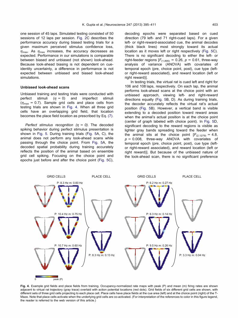
(gmax = 0.7). Sample grid cells and place cells from
testing trials are shown in Fig. 4. When all three grid
cells have an overlapping grid field, that location
becomes the place field location as prescribed by Eq. (7).
Perfect stimulus recognition (g = 0). The decoded
spiking behavior during perfect stimulus presentation is
shown in Fig. 5. During training trials (Fig. 5A, C), the
animal does not perform any look-ahead scans while
passing through the choice point. From Fig. 5A, the
decoded spatial probability during training accurately
reflects the position of the animal based on ensemble
grid cell spiking. Focusing on the choice point and
epochs just before and after the choice point (Fig. 5C),
GRID CELLS PLACE CELL
peak (P)0
P: 8.3 Hz m: 0.60 Hz
P: 10.4 Hz m: 0.75 Hz
P: 10.7 Hz m: 0.60 Hz
zH31.0:mzH3.8:P
Fig. 4. Example grid fields and place fields from training. Occupancy-norm
adjacent to virtual rat trajectory (gray trace) overlaid with action potential loc
different sets of three grid cells projecting to each place cell. Place cells have p
Maze. Note that place cells activate when the underlying grid cells are co-activ
the reader is referred to the web version of this article.)
decoding epochs were separated based on cued
direction (79 left- and 71 right-cued laps). For a given
left- or right-reward-associated cue, the animal decodes
(thick black lines) most strongly toward its actual
location as it moves left or right respectively (Fig. 5C).
There is no significant decoding to either the left- or
right-feeder regions [F(1,895) = 0.26, p= 0.61, three-way
analysis of variance (ANOVA) with covariates of
temporal epoch (pre, choice point, post), cue type (left-
or right-reward associated), and reward location (left or
right reward)].
In testing trials, the virtual rat is cued left and right for
106 and 108 laps, respectively. On each lap, the animal
performs look-ahead scans at the choice point with an
unbiased approach, viewing left- and right-reward
directions equally (Fig. 5B, D). As during training trials,
the decoder accurately reflects the virtual rat’s actual
position (Fig. 5B). However, a vertical band is visible
extending to a decoded position toward reward areas
when the animal’s actual position is at the choice point
(center of graph labeled with choice point). In Fig. 5D,
significant decoding to the reward regions is visible as
lighter gray bands spreading toward the feeder when
the animal sits at the choice point [F(2,1279) = 4.8,
p= 0.008, three-way ANOVA with covariates of
temporal epoch (pre, choice point, post), cue type (left-
or right-reward associated), and reward location (left or
right reward)]. But because of the unbiased nature of
the look-ahead scan, there is no significant preference
GRID CELLS PLACE CELL
P: 6.2 Hz m: 0.27 Hz
P: 6.3 Hz m: 0.14 Hz
P: 9.5 Hz m: 0.26 Hz
zH40.0:mzH3.3:P
alized rate maps with peak (P) and mean (m) firing rates are shown
ations (red dots). Grid fields of six different grid cells are shown, with
lace fields at the cue area (left) and at the choice point (right) of the T-
ated. (For interpretation of the references to color in this figure legend,

Cued LeftTurned Right
30 Laps
Cued RightTurned Left:
31 Laps
cue
choi
cepo
int
feed
er
cue
choicepoint
feeder
0
1
cue
choicepoint
feeder
cue
choi
cepo
int
feed
er
Dec
oded
Pos
ition
ActualPositionActualPosition
Training Trials(No Look-Ahead Probes Present)
Testing Trials(Look-Ahead Probes Present)
A
Decoding Probability
0
0.14
Decoding Probability
C
B
D
Left
Turn
Rig
ht T
urn
pre
choi
cepo
int
post pre
choi
cepo
int
post
Right Feeder
Left Feeder
Left Cue
Right Cue
Cued Left:79 Laps
Cued Right:71 Laps
pre
choi
cepo
int
post pre
choi
cepo
int
post
Right Feeder
Left Feeder
Left Cue
Right Cue
Cued Left:106 Laps
Cued Right:108 Laps
ηmax = 0.0
E
pre
choi
cepo
int
post pre
choi
cepo
int
post
Right Feeder
Left Feeder
Left Cue
Right Cue
Cued LeftTurned Left
70 Laps
Cued RightTurned Right
69 Laps
pre
choi
cepo
int
post pre
choi
cepo
int
post
Right Feeder
Left Feeder
Left Cue
Right Cue
ηmax = 0.7
F
20 40 60
Right Choice Point
Right Feeder
ActualDecoded
Cued Right
Time (sec)
Cued Left
Left Choice Point
Left Feeder
nruTthgiR
nr uTtfeL
Fig. 5. Spatial decoding of training trials and testing trials with unbiased look-ahead. (A) Decoded position from ensemble spiking during training
trials demonstrate accurate decoding to the actual position during spiking activity. (B) During testing trials, similar decoding accuracy is visible as in
(A), however, forward activation is visible with increased decoding at the choice point to the feeder (reward region) ahead of the choice point. (C) As
in (A), training trials show the same decoding accuracy zooming in on temporal epochs of 1 s before the choice point (‘pre’), at the choice point, and
1 s after the choice point (‘post’) for left- and right-reward cued trials (left and right panels, respectively). Black dashed line represents linear position
0 and tick marks on vertical axis indicate choice point locations on trajectory. (D) During unbiased look-ahead testing with gmax = 0.0, spatial
decoding probability at the choice point region shows comparable spatial decoding (gray lines marked with weighted arrows) to the left and right
reward areas given a left- or right-reward cued trial (left and right panels, respectively). (E) Similar to (D), unbiased testing with gmax = 0.7 yields
comparable decoding to the feeder regions when the animal traversed correctly (top panels) or incorrectly (bottom panel in gray) given a left- or
right-reward cued trial (left and right panels, respectively). (F) Right- and left-reward bound laps of cued behavior with actual (dashed gray line) and
decoded (black line) trajectories. The decoded trajectory tracks actual trajectory, except for jumps in decoded trajectory toward reward locations
when the animal sits at the choice point. Note the size of decoded jump does not indicate a magnitude of any kind. Rather, look-ahead probes in the
direction opposite the cued direction produce linearized coordinates with the opposite sign.
404 K. Gupta et al. / Neuroscience 247 (2013) 395–411

K. Gupta et al. / Neuroscience 247 (2013) 395–411 405
to decode to the left or right feeder given a left (p= 0.65,
two-tailed Student’s t-test) or right (p= 0.10, two-tailed
Student’s t-test) cue.Fig. 5B also shows a horizontal band of decoding to
the choice point region. This horizontal band indicates
that when the virtual rat is between the choice point and
the reward location, MEC neurons will contain spatial
information about the rat’s current location and the
choice point. Grid cells with firing fields between the
choice point and the reward locations spike in two
circumstances: (1) when the virtual rat or (2) a look-
ahead probe (where virtual rat pauses at choice point)
passes through the firing field. The decoder is trained
on epochs when these particular grid cells fire action
potentials. Because the virtual rat’s actual location can
either be at the grid field or the choice point when these
neurons spike, the decoder provides spatial information
for both locations.
Imperfect stimulus recognition (gmax = 0.7). Training
trials do not decode differently between perfect and
imperfect stimuli because no look-ahead scans are
present. The only notable difference across training
trials occurs within the matrix WS visible in Fig. 2A, B.
Testing trials are visible in Fig. 5E. The virtual animal
performed 200 laps, 139 correct (70 left- and 69 right-
cued) and 61 error trials (30 left- and 31 right-cued).
Like Fig. 5D, significant decoding to the reward regions
is visible spreading to the feeder when the animal sits at
the choice point [F(2,1194) = 6.95, p= 0.001, four-way
ANOVA with covariates of temporal epoch (pre, choice
point, post), cue type (left- or right-reward associated),
reward location (left or right reward), and epoch
accuracy (correct or incorrect)]. Again, because look-
ahead scans are unbiased, decoding to the left- or right
feeder does not differ whether the animal performed
correctly (left feeder given left cue: p= 0.54, right
feeder given right cue: p= 0.28, two-tailed Student’s t-test adjusted with Holm–Bonferroni correction) or
incorrectly (left feeder given right cue: p= 0.44, right
feeder given left cue: p= 0.37, two-tailed Student’s t-test adjusted with Holm-Bonferroni correction). Fig. 5F
shows decoded (peak spatial decoding probability
location) and actual trajectories of the virtual animal on
right- and left-reward bound laps over time. The jumps
in decoded trajectory from the choice point to the
reward locations as the animal sits at the choice point
represent forward activations during unbiased look-
ahead scans. For each lap, there are three scans to the
right- and left-reward locations. Look-ahead scans in the
direction opposite the cued direction produce linearized
coordinates with a sign opposite the trajectory
linearization, resulting in large jumps as shown.
Biased look-ahead
Spatial decoding is reported for biased test sessions with
gmax = 0.0 and gmax = 0.7. Temporal decoding is
reported below for biased test sessions with gmax = 0.7.
For gmax = 0.0, the virtual animal was cued left and
right 300 times each, performing correctly on every lap.
For gmax = 0.7, the virtual animal was cued left and
right 300 times each, performing correctly on 234 and
210 left- and right-cued laps, respectively, and
incorrectly on 66 and 90 left- and right-cued laps
respectively.
Perfect stimulus recognition (gmax = 0.0) spatialdecoding. With zero cue-identity uncertainty, the
stimulus Sp yields 100% performance (see Fig. 2). The
virtual animal correctly performed 600 laps with 300
trials each of left and right cues. Fig. 6A shows spatial
decoding probabilities when the animal’s trajectory is
pre-choice point, choice point, and post-choice point.
Like in Fig. 5D, E, significant decoding toward the
feeder regions is visible at the choice point
[F(2,3595) = 68.1, p< 0.0001, three-way ANOVA with
covariates of temporal epoch (pre, choice point, post),
cue type (left- or right-reward associated), and reward
location (left or right reward)]. However, unlike the
unbiased look-ahead simulations, significant asymmetry
is visible with stronger decoding to the left feeder
(p< 0.0001, two-tailed Student’s t-test) or right feeder
(p< 0.0001, two-tailed Student’s t-test) given a left or
right cue, respectively.
Imperfect stimulus recognition (gmax = 0.7) spatialdecoding. The presence of cue-identity uncertainty
induces errors in virtual rat performance. Decoding
epochs varied not only by cued direction (left or right),
but also by correct or incorrect choice point turn
direction. Figs. 5 and 6B demonstrate significant
decoding to reward locations at the choice point
[F(2,3594) = 166.0, p< 0.0001, four-way ANOVA with
covariates of temporal epoch (pre, choice point, post),
cue type (left- or right-reward associated), reward
location (left or right reward), and epoch accuracy
(correct or incorrect)]. The two top panels of Fig. 6B
demonstrate decoding for epochs where animals turned
in the correctly cued direction. The choice point epoch
(center column) shows strongest decoding (gray lines)
to the correct feeder location (left feeder given left
cue: p < 0.0001, right feeder given right cue:
p< 0.0001, two-tailed Student’s t-test adjusted with
Holm–Bonferroni correction), unlike in the unbiased
look-ahead scan of Fig. 5. Decoding the representation
at the choice point before the animal turns in the
incorrect direction (Fig. 6B, bottom panels) shows that
the feeder location associated with the incorrect turn
has the strongest spatial decoding as evident from the
gray lines in the center column (right feeder given left
cue: p < 0.0001, left feeder given right cue:
p< 0.0001, two-tailed Student’s t-test adjusted with
Holm–Bonferroni correction).
Comparison to in vivo data. The specific examples of
unbiased and biased look-ahead testing simulations
have qualitatively appeared similar to the in vivo data
shown in Fig. 6C. Using a 2-D Pearson’s Correlation
Coefficient between the in vivo and simulation decoding
probabilities, Table 1 describes quantitatively how well
the virtual experiments fit the unit recording decoding
analysis. For simulations where the animal turns

Cued LeftTurned Correctly Left
Cued RightTurned Correctly Right
Cued LeftTurned Incorrectly Right
Cued RightTurned Incorrectly Left
0
0.14
Decoding P
robability
B
model spatial decoding (ηmax = 0.7)
Left
Turn
Rig
ht T
urn
Right Feeder
Left Feeder
Left Cue
Right Cue
pre
choi
cepo
int
post
pre
choi
cepo
int
post
Right Feeder
Left Feeder
Left Cue
Right Cue
pre
choi
cepo
int
post
pre
choi
cepo
int
post
in vivo data spatial decoding(Gupta et al., 2012)
Cued LeftTurned Correctly Left
Cued RightTurned Correctly Right
Cued LeftTurned Incorrectly Right
Cued RightTurned Incorrectly Left
0
0.06
Decoding P
robability
CLe
ft Tu
rnR
ight
Tur
n
Right Feeder
Left Feeder
Left Cue
Right Cuepr
ech
oice
poin
tpo
st
pre
choi
cepo
int
post
Right Feeder
Left Feeder
Left Cue
Right Cue
pre
choi
cepo
int
post
pre
choi
cepo
int
post
Cued LeftTurned Correctly Left
Cued RightTurned Correctly Right
0
0.14
Decoding P
robability
A
Right Feeder
Left Feeder
Left Cue
Right Cue
pre
choi
cepo
int
post
pre
choi
cepo
int
post
model spatial decoding (ηmax = 0.0)
Left
Turn
Rig
ht T
urn
Fig. 6. (A) Spatial decoding of biased look-ahead testing for gmax = 0.0. Two decoding epochs are shown varied by cue direction (left or right).
Stronger decoding is visible when the virtual animal is at the choice point to left- or right-feeder given a left- or right-reward associated cue,
respectively (gray lines marked with weighted arrows). Black dashed line represents linear position 0 and tick marks on vertical axis indicate choice
point locations on trajectory. (B) Spatial decoding of testing trials with biased look-ahead for gmax = 0.7. Four decoding epochs are shown varied by
cue direction (left or right) and correct (top panels) or incorrect (bottom panels in gray) turning direction. Correct trials decode strongly to the left (top
left panel) or right (top right panel) feeder location when the animal is cued left or right, respectively (gray lines marked with weighted arrows). Error
trials decode strongly to the left (bottom right panel) or right (bottom left panel) feeder location given a right or left cue, respectively (gray lines
marked with weighted arrows). (C) Similar spatial decoding profiles from in vivo data (from Gupta et al., 2012) with epochs varied by cued direction
(left or right) and correct (top panels) or incorrect (bottom panels in gray) turning direction.
406 K. Gupta et al. / Neuroscience 247 (2013) 395–411

Table 1. Correlation coefficients of spatial decoding probabilities of simulated testing (with biased or unbiased look-ahead scans) to in vivo decoding
probabilities shown in Fig. 6C, given different cue-identity uncertainties. Note: simulations with gmax 6 0.5 do not generate significant numbers of error
laps, so comparisons are only made on correct behavioral epochs
Cue-identity
uncertainty (gmax)
Spatial decoding epochs
Cued left
Turned correctly left
Cued right
Turned correctly right
Cued left
Turned incorrectly right
Cued right
Turned incorrectly left
Biased
look-ahead
Unbiased
look-ahead
Biased
look-ahead
Unbiased
look-ahead
Biased
look-ahead
Unbiased
look-ahead
Biased
look-ahead
Unbiased
look-ahead
1.0 0.46 0.43 0.31 0.18 0.32 0.38 0.22 0.33
0.9 0.46 0.42 0.32 0.19 0.32 0.37 0.23 0.33
0.8 0.47 0.40 0.33 0.20 0.34 0.38 0.22 0.34
0.7 0.48 0.43 0.32 0.21 0.33 0.38 0.21 0.35
0.6 0.49 0.43 0.30 0.19 0.38 0.40 0.29 0.35
0.5 0.51 0.45 0.33 0.20
0.4 0.51 0.45 0.32 0.20
0.3 0.40 0.44 0.28 0.21
0.2 0.40 0.44 0.25 0.21
0.1 0.50 0.44 0.33 0.20
0.0 0.47 0.43 0.35 0.21
K. Gupta et al. / Neuroscience 247 (2013) 395–411 407
correctly at the choice point, biased look-ahead
simulations correlate better to the in vivo data than
unbiased simulations (cued left, turned correctly left:
p= 0.009; cued right, turned correctly right:
p< 0.0001; Student’s t-test with Holm–Bonferroni
correction). When the virtual rat errors at the choice
point, unbiased look-ahead simulations correlate better
to the in vivo data than biased simulation (cued left,
turned incorrectly right: p= 0.007; cued right, turned
incorrectly left: p= 0.002; Student’s t-test with Holm–
Bonferroni correction). Part of Table 1 is empty for
simulations where gmax 6 0.5. In these table positions,
the simulations do not produce enough error trials to
make any comparisons.
Temporal decoding. Similar to Fig. 6B, where spatial
decoding epochs varied by cued direction (left or right)
and correct or incorrect choice point turn direction, the
temporal decoder varied its decoding epochs yielding
the four plots in Fig. 7. Fig. 7A, D demonstrate the
probability of decoding to ‘time from left feeder’ and
Fig. 7B, C show decoding to ‘time from right feeder.’
Temporal decoding probability significantly differs from
the choice point to pre- and post-choice point epochs
[F(2,1795) = 53.6, p< 0.0001, three-way ANOVA with
covariates of temporal epoch (pre, choice point, post),
cue type (left- or right-reward associated), and epoch
accuracy (correct or incorrect)]. During pre- and post-
choice point epochs, the virtual rat does not perform a
look-ahead scan. The only spiking seen at these times
are from grid cells whose fields the animal passes
through. Because grid fields are generated with differing
periodicities along the stem (pre-choice point) and in the
reward arms (post-choice point), the spiking they elicit
reflects the banding pattern seen in the temporal
decoding. At the choice point, however, spiking occurs
when the look-ahead probe passes over persistent
spiking cells, grid cells, and place cells. The temporal
decoding shows relatively high decoding probabilities to
all times prior the virtual rat’s entry to the reward zones.
Decoding probability drops to 0 for all times after time
t= 0 because our implementation of the look-ahead
probe does not scan place cells farther ahead in time
beyond the reward regions. If in vivo temporal decoding
probability does not drop to 0 after times ahead of the
reward region, then that is indicative of longer-lasting
look-ahead scanning.
DISCUSSION
This article presents an updated version of the model of
Erdem and Hasselmo (2012) focusing on grid cells
activity as a virtual rat runs a cued, appetitive T-Maze
task. In vivo data (see Fig. 6B) suggests that medial
entorhinal neurons are capable of performing look-
ahead functions on such tasks, where ensemble activity
indicates perception of spatial locations forward from the
animal’s current position (Gupta et al., 2012). The
model presented here trains a virtual rat to associate
reward with perfect and imperfect cue stimuli, an update
on the previous model. The cognitive map the animal
develops over training associates place cells to reward
cells that are activated given the appropriate cue. At the
choice point, the animal performs look-ahead scans in
both rewarded directions, triggering action potentials
from cells along those scanned trajectories (e.g.
persistent spiking cells, grid cells, and place cells). The
virtual animal employs both biased and unbiased look-
ahead probes, with the former strategy better modeling
epochs where animals turned correctly, and with the
latter strategy better for epochs where animals turned
incorrectly. Each look-ahead strategy produces forward
activations from the choice point to the feeder locations
as the animal pauses. Temporal decoding further
validates the model showing that look-ahead scans are
constantly activating the grid cell network when the
animal sits at the choice point deliberating which
direction to take, compared to pre- and post-choice
point epochs.

Cued Left, Turned Correctly Left
5
0
-5
-10
-15
pre
choi
cepo
int
post
Tim
e Fr
om L
eft F
eede
r (s)
Cued Right, Turned Correctly Right
pre
choi
cepo
int
post
5
0
-5
-10
-15
Tim
e Fr
om R
ight
Fee
der (
s)
0
0.06
Decoding Probability
BA
Cued Left,Turned Incorrectly Right
5s)
C Cued Right,Turned Incorrectly Left
5
)
D
408 K. Gupta et al. / Neuroscience 247 (2013) 395–411
Cue-to-reward connection matrix
The current model incorporates a learning rule for both
certain (perfect) and uncertain (imperfect) cue identities.
The Hebbian associations between reward cells and cue
stimuli develop over multiple training laps and continue
during testing sessions. This feature significantly adds
to Erdem and Hasselmo (2012) by allowing for learned
cues during training to drive future choices. Without
these learned associations, the virtual rat would not be
able to identify which recruited place cells and
associated reward cells should be encoded with a given
cue. Such cue-reward associations have been modeled
previously using reinforcement learning (Sutton and
Barto, 1998) implementing a value-state system
(Hasselmo and Eichenbaum, 2005; Zilli and Hasselmo,
2008) for the virtual rat. Our implementation relies on
Hebbian cue-reward associations that retrieve reward
cells (and reward-associated place cells). The retrieved
reward-associated place cell is activated as a look-
ahead probe passes through the cell’s place field. It is
this feature that makes look-ahead agnostic to the
actual mechanism of place cell retrieval, so long as the
correct goal-associated place cell is retrieved by the
time the virtual rat arrives at the choice point to begin
scanning.
0-5
-10
-15
Tim
e Fr
om R
ight
Fee
der (
pre
choi
cepo
int
post pre
choi
cepo
int
post
0
-5
-10
-15
Tim
e Fr
om L
eft F
eede
r (s
Fig. 7. Temporal decoding to times before triggering the left or right
feeder. Panels (A) and (D) represent decoding to ‘time from left
feeder activation’ (time t= 0) when the virtual animal turns correctly
or incorrectly toward left reward, respectively. Panels (B, C) are
similar representations for ‘time from right feeder activation’ (time
t= 0) when the virtual animal turns correctly or incorrectly toward
right reward, respectively. Band patterns are visible when the virtual
rat occupies pre- and post-choice point regions. Here, the virtual
animal is not performing look-ahead scans, but is running through
grid fields. At the choice point, the virtual rat performs multiple look-
ahead scans prior to running to the reward site visible via elevated
decoding probability up to t= 0.
Implications of spatial and temporal decoding results
Throughout our simulations, we assumed the virtual rat
performed a look-ahead scan only while pausing at the
choice point. Fig. 6B explicitly shows that the choice
point region is the prime location where non-local
representations occur similar to those seen in vivo
(Fig. 6C). Furthermore, the spatial decoding at the
choice point is limited to locations up to the reward
regions. The temporal decoding corroborates this
assumption by showing consistent probability of
decoding to a time before triggering reward while the
animal sits at the choice point (Fig. 7). Our assumptions
in the model simplify computational complexity, but it
captures only part of the in vivo data. Gupta et al.
(2012) show ensembles of medial entorhinal neurons
decoding to appropriately cued reward locations during
correct trials (Fig. 6C). However, low-level, non-local
noisy decoding to all other regions is present, similar to
spatial decoding in the hippocampus (Johnson and
Redish, 2007) and ventral striatum (van der Meer and
Redish, 2009). In addition, decoding in the ventral
striatum demonstrates ensembles decoding temporally
beyond the feeder, typically by 2 to 4s (van der Meer
and Redish, 2009).
These results suggest three considerations for our
simulations. First, animals must be performing look-
ahead scans at various times, not just when pausing at
the choice point. The look-ahead scan need not limit
itself to just the reward locations. This point is
particularly interesting because it depends on how much
of the route facing the virtual animal can be sensed. If
the animal could sense (visually or otherwise), regions
advanced from the reward trigger, then the look-ahead
probe need not be straight line probes as we have
implemented. By placing high walls to visually obscure
T-Maze reward locations, in vivo manipulations could
determine whether visual information is the predominant
sensory modality for look-ahead scans.
Second, our model assumes noiseless spatial
navigation. We do not introduce phasic noise into
persistent spiking cells or VCOs, thereby eliminating
significant noise sources for the grid and place cell
system. Additionally, we treat place fields as a
superposition of three underlying grid fields, which may
not be the case especially given evidence from

K. Gupta et al. / Neuroscience 247 (2013) 395–411 409
trajectory-dependent place cell (Wood et al., 2000) and
grid cell firing (Lipton et al., 2007) and grid field
fragmentation (Derdikman et al., 2009; Gupta et al.,
2013). In these experiments, animals perform a
cognitive task in 1-D mazes, which confer different
cognitive demands than foraging behavior in 2-D
environments. Furthermore, 1-D maze geometry may
induce complex resetting of the spatial navigation
system not necessarily present in 2-D open field arenas.
Third, the reward layer we employ does not
necessarily need to be a part of the PFC. Though
considerable evidence makes the PFC a likely
candidate structure, studies from the ventral striatum
also make it a likely candidate. Forward activation in
cued choice tasks has been seen in neuronal
ensembles from the ventral striatum (van der Meer and
Redish, 2009) which may represent decision-making
expectations (van der Meer and Redish, 2010). In
addition, intrinsic firing of ventral striatal neurons show
stronger coherence to hippocampal theta rhythm, with
phase precession associated with anticipatory firing to
reward locations (van der Meer and Redish, 2011).
Unbiased and biased look-ahead strategies
The look-ahead scan offers a mechanism for animals to
verify learned choices, like during VTE (Muenzinger,
1938; Hu and Amsel, 1995; Johnson and Redish, 2007).
VTE events typically show a biased approach toward a
direction as the animal deliberates the correct decision
to take. During error trials, however, a biased approach
is less apparent as animals demonstrate equivalent
forward activations to either correct or incorrect reward
locations (Gupta et al., 2012). Animals may use a
biased approach when they are more confident of the
correctly reward location, eliminating the need to inspect
an incorrect reward location. With increased uncertainty
about which direction to take, scanning both reward
locations becomes more important. The results of
Table 1 suggest that the model presented can
adequately emulate the shift from unbiased to biased
look-ahead based on whether the animal moves to the
correct reward location.
Hippocampal replay, visible during epochs of LFP
sharp-wave ripples in quiescent states (Wilson and
McNaughton, 1994; Louie and Wilson, 2001; Karlsson
and Frank, 2009), has also shown bias toward
hippocampal events associated with learned cues that
are later played while animals sleep (Bendor and
Wilson, 2012). In our implementation of bias, we applied
a constant bias dependent on the animal’s connection
matrix between reward location and choice. This yielded
a similar bias for look-ahead regardless of the cue-
identity uncertainty of the perceived stimulus. However,
this constant bias could be modified to include a time-
dependent biasing that scales with stimulus uncertainty.
This would imply that as the uncertainty term gmax
increases, the look-ahead scans will scan left and right
rewards with increasingly equal probabilities.
We could implement the bias direction selection using
a partially observable Markov decision process (Zilli and
Hasselmo, 2008). Our current strategy using Hebbian
learning-associating cue and bias direction does not
take into account the state of the virtual rat. At each
location the rat visits, a value (derived from previous
states and reward visits) could be associated with the
location comprising the state of the animal at that time
and place. Cue presentation could retrieve the animal’s
state which would include a probability of selecting the
left- or right-reward. The time from cue presentation
would then affect the probability based on the number of
states the animal must pass through to achieve reward.
When animals become more confident about cue-
reward associations, the need for look-ahead scans
likely diminishes. In tasks such as continuous spatial
alternation, animals can complete each lap in a brief
instant with a high degree of accuracy across sessions
(Frank et al., 2000; Wood et al., 2000; Lipton et al.,
2007), even with damage to the hippocampus (Ainge
et al., 2007). In the delayed version of spatial
alternation, the hippocampus is necessary to perform
the task (Ainge et al., 2007) suggesting that the
underlying place cell circuit must be intact to
successfully navigate the increased complexity.
Furthermore, the delayed version of this task also elicits
phasic anticipatory elevations of PFC dopamine and
noradrenaline correlated to reward expectancy and
active maintenance of goal information, respectively
(Rossetti and Carboni, 2005). The intact reward cell and
place cell layers employed during delayed spatial
alternation suggest that look-ahead probes may be
useful during the delay period to disambiguate the
forward route.
Although we emphasize the prospective spatial
information encoded by MEC ensembles, the output of
the Bayesian decoder possibly suggests a retrospective
mode. The horizontal band of decoding seen in Fig. 5B,
as mentioned earlier, is a product of training the
decoder from grid cells with firing fields between the
choice point and the reward locations. Because grid
cells with firing fields between these two locations will
fire when the virtual animal is either at the choice point
or passing through the grid field, spiking must contain
spatial information about both locations. Other studies
have also noted similar symmetry across the main
diagonal similar to Fig. 5B (van der Meer and Redish,
2009). It is possible that this horizontal band could be a
mechanism for retrospective activity seen in grid cells
(De Almeida et al., 2012). Here, grid cells spiked more
frequently either inbound toward (prospective mode) or
outbound from (retrospective mode) a grid field vertex.
The memory mode was consistent across cells for
vertex crossings less than a second apart indicating that
such memory modes may be dependent on a network
of cells. If the network behaves like a Bayesian decoder,
the horizontal band observed in Fig. 5B may contribute to
the retrospective mode.
The overall architecture of the model has several
benefits for cued behavior. Because we do not
necessarily require reward diffusion to perform
behavioral tasks, we are able to maintain a sparse place
field representation of the environment, only requiring
representations of task-relevant locations like the reward

410 K. Gupta et al. / Neuroscience 247 (2013) 395–411
areas and turning points. The only inputs to the system at
any time, heading and speed information, activate the grid
cell and place cell layers to transduce location and
retrieve reward-associated information. The model using
biased look-ahead is able to replicate the decoding of
neurophysiological data (Fig. 6C) showing activity for
the reward location when the animal is at the choice
point. The look-ahead probe’s ability to assist in
diminishing uncertainty makes it a vital part of any goal-
directed navigation with significant ambiguity.
Acknowledgements—The authors would like to thank Andrew R.
Bogaard for programming assistance. This work was supported
by the National Institute of Mental Health grants (MH60013 and
MH61492) and the Office of Naval Research Multidisciplinary
University Initiative grant N00014-10-1-0936 awarded to Michael
E. Hasselmo.
REFERENCES
Adams AD, Forrester JM (1968) The projection of the rat’s visual field
on the cerebral cortex. Q J Exp Physiol Cogn Med Sci
53:327–336.
Ainge JA, van der Meer MA, Langston RF, Wood ER (2007)
Exploring the role of context-dependent hippocampal activity in
spatial alternation behavior. Hippocampus 17:988–1002.
Bendor D, Wilson MA (2012) Biasing the content of hippocampal
replay during sleep. Nat Neurosci 15:1439–1444.
Blair HT, Gupta K, Zhang K (2008) Conversion of a phase- to a rate-
coded position signal by a three-stage model of theta cells, grid
cells, and place cells. Hippocampus 18:1239–1255.
Brandon MP, Bogaard AR, Libby CP, Connerney MA, Gupta K,
Hasselmo ME (2011) Reduction of theta rhythm dissociates grid
cell spatial periodicity from directional tuning. Science
332:595–599.
Brandon MP, Bogaard AR, Andrews CM, Hasselmo ME (2012) Head
direction cells in the postsubiculum do not show replay of prior
waking sequences during sleep. Hippocampus 22:604–618.
Burgess N (2008) Grid cells and theta as oscillatory interference:
theory and predictions. Hippocampus 18:1157–1174.
Burgess N, Donnett JG, Jeffery KJ, O’Keefe J (1997) Robotic and
neuronal simulation of the hippocampus and rat navigation. Philos
Trans R Soc Lond B Biol Sci 352:1535–1543.
Burgess N, Barry C, O’Keefe J (2007) An oscillatory interference
model of grid cell firing. Hippocampus 17:801–812.
Burton BG, Hok V, Save E, Poucet B (2009) Lesion of the ventral and
intermediate hippocampus abolishes anticipatory activity in the
medial prefrontal cortex of the rat. Behav Brain Res 199:222–234.
Canto CB, Wouterlood FG, Witter MP (2008) What does the
anatomical organization of the entorhinal cortex tell us? Neural
Plast 2008:381243.
De Almeida L, Idiart M, Villavicencio A, Lisman J (2012) Alternating
predictive and short-term memory modes of entorhinal grid cells.
Hippocampus 22:1647–1651.
Derdikman D, Whitlock JR, Tsao A, Fyhn M, Hafting T, Moser MB,
Moser EI (2009) Fragmentation of grid cell maps in a
multicompartment environment. Nat Neurosci 12:1325–1332.
Duff A, Fibla MS, Verschure PF (2011) A biologically based model for
the integration of sensory-motor contingencies in rules and plans:
a prefrontal cortex based extension of the distributed adaptive
control architecture. Brain Res Bull 85:289–304.
Erdem UM, Hasselmo M (2012) A goal-directed spatial navigation
model using forward trajectory planning based on grid cells. Eur J
Neurosci 35:916–931.
Ferbinteanu J, Shapiro ML (2003) Prospective and retrospective
memory coding in the hippocampus. Neuron 40:1227–1239.
Frank LM, Brown EN, Wilson M (2000) Trajectory encoding in the
hippocampus and entorhinal cortex. Neuron 27:169–178.
Fyhn M, Molden S, Witter MP, Moser EI, Moser MB (2004) Spatial
representation in the entorhinal cortex. Science 305:1258–1264.
Gupta AS, van der Meer MA, Touretzky DS, Redish AD (2010)
Hippocampal replay is not a simple function of experience.
Neuron 65:695–705.
Gupta K, Keller LA, Hasselmo ME (2012) Reduced spiking in
entorhinal cortex during the delay period of a cued spatial
response task. Learn Mem 19:219–230.
Gupta K, Beer NJ, Keller LA, Hasselmo ME (2013) Medial entorhinal
grid cells and head direction cells rotate with a T-Maze more often
during less recently experienced rotations. Cereb Cortex. http://
dx.doi.org/10.1093/cercor/bht020.
Hafting T, Fyhn M, Molden S, Moser MB, Moser EI (2005)
Microstructure of a spatial map in the entorhinal cortex. Nature
436:801–806.
Hargreaves EL, Yoganarasimha D, Knierim JJ (2007) Cohesiveness
of spatial and directional representations recorded from neural
ensembles in the anterior thalamus, parasubiculum, medial
entorhinal cortex, and hippocampus. Hippocampus 17:826–841.
Hasselmo ME (2008a) Grid cell mechanisms and function:
contributions of entorhinal persistent spiking and phase
resetting. Hippocampus 18:1213–1229.
Hasselmo ME (2008b) Temporally structured replay of neural activity
in a model of entorhinal cortex, hippocampus and postsubiculum.
Eur J Neurosci 28:1301–1315.
Hasselmo ME, Eichenbaum H (2005) Hippocampal mechanisms for
the context-dependent retrieval of episodes. Neural Netw
18:1172–1190.
Hok V, Save E, Lenck-Santini PP, Poucet B (2005) Coding for spatial
goals in the prelimbic/infralimbic area of the rat frontal cortex.
Proc Natl Acad Sci U S A 102:4602–4607.
Hok V, Lenck-Santini PP, Roux S, Save E, Muller RU, Poucet B
(2007) Goal-related activity in hippocampal place cells. J Neurosci
27:472–482.
Hu D, Amsel A (1995) A simple test of the vicarious trial-and-error
hypothesis of hippocampal function. Proc Natl Acad Sci U S A
92:5506–5509.
Huang Y, Brandon MP, Griffin AL, Hasselmo ME, Eden UT (2009)
Decoding movement trajectories through a T-maze using point
process filters applied to place field data from rat hippocampal
region CA1. Neural Comput 21:3305–3334.
Hyman JM, Zilli EA, Paley AM, Hasselmo ME (2005) Medial
prefrontal cortex cells show dynamic modulation with the
hippocampal theta rhythm dependent on behavior.
Hippocampus 15:739–749.
Johnson A, Redish AD (2007) Neural ensembles in CA3 transiently
encode paths forward of the animal at a decision point. J Neurosci
27:12176–12189.
Jones MW, Wilson MA (2005a) Phase precession of medial prefrontal
cortical activity relative to the hippocampal theta rhythm.
Hippocampus 15:867–873.
Jones MW, Wilson MA (2005b) Theta rhythms coordinate
hippocampal–prefrontal interactions in a spatial memory task.
PLoS Biol 3:e402.
Karlsson MP, Frank LM (2009) Awake replay of remote experiences
in the hippocampus. Nat Neurosci 12:913–918.
Kubie JL, Fenton AA (2012) Linear look-ahead in conjunctive cells: an
entorhinal mechanism for vector-based navigation. Front Neural
Circuits 6:20.
Lee DN, Reddish PE (1981) Plummeting gannets: a paradigm of
ecological optics. Nature 293:293–294.
Lee AK, Wilson MA (2002) Memory of sequential experience in the
hippocampus during slow wave sleep. Neuron 36:1183–1194.
Lipton PA, White JA, Eichenbaum H (2007) Disambiguation of
overlapping experiences by neurons in the medial entorhinal
cortex. J Neurosci 27:5787–5795.
Louie K, Wilson MA (2001) Temporally structured replay of awake
hippocampal ensemble activity during rapid eye movement sleep.
Neuron 29:145–156.

K. Gupta et al. / Neuroscience 247 (2013) 395–411 411
McNaughton BL, Battaglia FP, Jensen O, Moser EI, Moser MB (2006)
Path integration and the neural basis of the ‘cognitive map’. Nat
Rev Neurosci 7:663–678.
Morris RG, Garrud P, Rawlins JN, O’Keefe J (1982) Place navigation
impaired in rats with hippocampal lesions. Nature 297:681–683.
Muenzinger KF (1938) Vicarious trial and error at a point of choice: I.
A general survey of its relation to learning efficiency. Pedagog
Semin J Genet Psychol 53:75–86.
O’Keefe J, Burgess N (1996) Geometric determinants of the place
fields of hippocampal neurons. Nature 381:425–428.
O’Keefe J, Burgess N (2005) Dual phase and rate coding in
hippocampal place cells: theoretical significance and
relationship to entorhinal grid cells. Hippocampus 15:853–866.
O’Keefe J, Dostrovsky J (1971) The hippocampus as a spatial map.
Preliminary evidence from unit activity in the freely-moving rat.
Brain Res 34:171–175.
Raudies F, Hasselmo ME (2012) Modeling boundary vector cell firing
given optic flow as a cue. PLoS Comput Biol 8:e1002553.
Raudies F, Mingolla E, Hasselmo ME (2012) Modeling the influence
of optic flow on grid cell firing in the absence of other cues1. J
Comput Neurosci 33:475–493.
Redish AD, Touretzky DS (1998) The role of the hippocampus in
solving the Morris water maze. Neural Comput 10:73–111.
Rossetti ZL, Carboni S (2005) Noradrenaline and dopamine
elevations in the rat prefrontal cortex in spatial working memory.
J Neurosci 25:2322–2329.
Sargolini F, Fyhn M, Hafting T, McNaughton BL, Witter MP, Moser
MB, Moser EI (2006) Conjunctive representation of position,
direction, and velocity in entorhinal cortex. Science 312:758–762.
Solstad T, Moser EI, Einevoll GT (2006) From grid cells to place cells:
a mathematical model. Hippocampus 16:1026–1031.
Steffenach HA, Witter M, Moser MB, Moser EI (2005) Spatial memory
in the rat requires the dorsolateral band of the entorhinal cortex.
Neuron 45:301–313.
Sutherland GR, McNaughton B (2000) Memory trace reactivation in
hippocampal and neocortical neuronal ensembles. Curr Opin
Neurobiol 10:180–186.
Sutton RS, Barto AG (1998) Reinforcement learning (adaptive
computation and machine learning). Cambridge, MA: MIT Press.
Taube JS (1995) Head direction cells recorded in the anterior
thalamic nuclei of freely moving rats. J Neurosci 15:70–86.
Taube JS, Muller RU, Ranck Jr JB (1990a) Head-direction cells
recorded from the postsubiculum in freely moving rats. I
Description and quantitative analysis. J Neurosci 10:420–435.
Taube JS, Muller RU, Ranck Jr JB (1990b) Head-direction cells
recorded from the postsubiculum in freely moving rats. II Effects
of environmental manipulations. J Neurosci 10:436–447.
van der Meer MA, Redish AD (2009) Covert expectation-of-reward in
rat ventral striatum at decision points. Front Integr Neurosci 3:1.
van der Meer MA, Redish AD (2010) Expectancies in decision
making, reinforcement learning, and ventral striatum. Front
Neurosci 4:6.
van der Meer MA, Redish AD (2011) Theta phase precession in rat
ventral striatum links place and reward information. J Neurosci
31:2843–2854.
Wilson MA, McNaughton BL (1994) Reactivation of hippocampal
ensemble memories during sleep. Science 265:676–679.
Wood ER, Dudchenko PA, Robitsek RJ, Eichenbaum H (2000)
Hippocampal neurons encode information about different types of
memory episodes occurring in the same location. Neuron
27:623–633.
Zhang K, Ginzburg I, McNaughton BL, Sejnowski TJ (1998)
Interpreting neuronal population activity by reconstruction:
unified framework with application to hippocampal place cells. J
Neurophysiol 79:1017–1044.
Zhang X, Sun C, Zheng N, Chen W, Zheng X (2012) Motion states
extraction with optical flow for rat-robot automatic navigation. Conf
Proc IEEE Eng Med Biol Soc 2012:976–979.
Zilli EA (2012) Models of grid cell spatial firing published 2005–2011.
Front Neural Circuits 6:16.
Zilli EA, Hasselmo ME (2008) Modeling the role of working memory
and episodic memory in behavioral tasks. Hippocampus
18:193–209.
(Accepted 26 April 2013)(Available online 7 May 2013)