Modeling of heat transfer and reactive chemistry for

Graduate Theses, Dissertations, and Problem Reports

2011

Modeling of heat transfer and reactive chemistry for particles in Modeling of heat transfer and reactive chemistry for particles in

gas-solid flow utilizing continuum-discrete methodology (CDM) gas-solid flow utilizing continuum-discrete methodology (CDM)

Jordan M. H. Musser West Virginia University

Follow this and additional works at: https://researchrepository.wvu.edu/etd

Recommended Citation Recommended Citation Musser, Jordan M. H., "Modeling of heat transfer and reactive chemistry for particles in gas-solid flow utilizing continuum-discrete methodology (CDM)" (2011). Graduate Theses, Dissertations, and Problem Reports. 4760. https://researchrepository.wvu.edu/etd/4760

This Dissertation is protected by copyright and/or related rights. It has been brought to you by the The Research Repository @ WVU with permission from the rights-holder(s). You are free to use this Dissertation in any way that is permitted by the copyright and related rights legislation that applies to your use. For other uses you must obtain permission from the rights-holder(s) directly, unless additional rights are indicated by a Creative Commons license in the record and/ or on the work itself. This Dissertation has been accepted for inclusion in WVU Graduate Theses, Dissertations, and Problem Reports collection by an authorized administrator of The Research Repository @ WVU. For more information, please contact [email protected].

https://researchrepository.wvu.edu/

https://researchrepository.wvu.edu/

https://researchrepository.wvu.edu/etd

https://researchrepository.wvu.edu/etd?utm_source=researchrepository.wvu.edu%2Fetd%2F4760&utm_medium=PDF&utm_campaign=PDFCoverPages

https://researchrepository.wvu.edu/etd/4760?utm_source=researchrepository.wvu.edu%2Fetd%2F4760&utm_medium=PDF&utm_campaign=PDFCoverPages

mailto:[email protected]

Modeling of heat transfer and reactive chemistry for particles in gas-solid flow

utilizing continuum-discrete methodology (CDM)

Jordan M. H. Musser

Dissertation submitted to the Eberly College of Arts and Sciences

at West Virginia University

in partial fulfillment of the requirements

for the degree of

Doctor of Philosophy

in

Mathematics

Approved by

Mary Ann Clarke, Ph.D., Committee Chairperson

Sherman Riemenschneider, Ph.D.

Ian Christie, Ph.D.

Edgar Fuller, Ph.D.

Janine Galvin, Ph.D.

Department of Mathematics

Morgantown, West Virginia

2011

Keywords: discrete element method, particle-scale modeling, gas-solids systems,

particle heat transfer

Copyright: 2011 Jordan M. H. Musser

Abstract

Modeling of heat transfer and reactive chemistry for particles in gas-solid flow

utilizing continuum-discrete methodology (CDM)

by Jordan M. H. Musser

A comprehensive multi-phase flow model requires coupled hydrodynamics,

boundary conditions, heat and mass transfer, and chemical reaction kinetics. A model

must also capture the multi-scale nature of these problems. Computational fluid

dynamics-discrete element method (CFD-DEM) provides an accurate description of

chemical reactions and heat and mass transfer at the particle scale. Currently, MFIX-

DEM, the existing CFD-DEM used as the foundation for this work, can only model

coupled hydrodynamics. This dissertation extends the functionality of MFIX-DEM by

addressing the remaining deficiencies in three separate efforts.

The first effort outlined in this dissertation focuses on the algorithmic

development of discrete mass inflow and outflow boundary conditions. This approach

allows for the construction of more dynamic models of gas-solid systems. It permits the

amount and type of particles to fluctuate during a simulation. Examples illustrating the

added functionality are provided.

The second investigation explores the three modes of heat transfer in gas-solids

systems. Models for particle-particle contact conduction, particle-fluid-particle

conduction, particle-gas convection, and particle-particle radiation are selected. Model

selection is based on model simplicity, acceptance in existing CFD-DEM heat transfer

models, extendibility to particles of different sizes, and computational expense.

Modifications are made to selected models before implementing them into MFIX-DEM.

The implementation of each model is verified for simple two particle test cases, or in the

case of gas-particle convection, a single fixed particle in a flowing gas. Strong agreement

is observed between the simulation data and the analytic or numerical solution.

Finally, a mathematical interface for managing user-defined particle-gas chemical

reactions is developed. The shrinking, unreacted core model is selected as the particle

reaction model for its accurate physical account of particle-gas reactions and ability to

allow particles to initially contain inert material. The implementation of the reactive

chemistry interface is verified for a single reacting particle. Strong agreement is observed

between simulation data and the analytic solutions for the particle’s mass, species mass

fraction, and internal energy equations. Agreement between the simulation data and

analytic solution for the shrinking, unreacted core is considered acceptable.

iii

Acknowledgements

I would first like to thank those responsible for funding this project. This was

provided by the National Energy Technology Laboratory (NETL) Research Participation

Program sponsored by the U.S. Department of Energy and administered by the Oak

Ridge Institute for Science and Education (ORISE). Without this contribution, this

project would not have been possible.

Collaborative support was provided by the developers of MFIX including (in

alphabetical order) Sofian Benyahia, Janine Carney, Jeff Dietiker, Rahul Garg, Aytekin

Gel, Chris Guenther, Tingwen Li, Philip Nicoletti, Tom O’Brien, Mehrdad Shahnam, and

Madhava Syamlal. I want to especially thank Janine Carney for all of her support and

insight throughout this entire project. Without her guidance and knowledge, this work

would have been insurmountable.

Many thanks go to my advisor Mary Ann Clarke. Although she may be the

Empress of Evil, Destroyer of Worlds to some (namely undergraduates), she has been and

will continue to be, a positive influence in my life. I am greatly appreciative of the

support and friendship Mary Ann and Michael have provided me over the years.

I would finally like to thank my friends and family. Thank you for not locking me

up in the ‘nut barn’ after 10+ years of college. Joe Andria also deserves special

recognition. Thank you for the countless opportunities to rant and rave about trivial

details in my course work and research. Thank you for all the clean laundry, tasty

dinners, and fun times we’ve shared over the year. You and your friendship is greatly

appreciated even though I may not say it enough.

iv

Table of Contents

Abstract .............................................................................................................................. ii

Acknowledgements .......................................................................................................... iii

Table of Contents ............................................................................................................. iv

List of Figures ................................................................................................................. viii

List of Tables .................................................................................................................. xiv

Nomenclature .................................................................................................................. xv

Abbreviations and Acronyms ....................................................................................... xxi

Chapter 1 : Introduction ................................................................................................. 1 1.1 CFD-Discrete element method (CFD-DEM) ............................................................ 2

1.1.1 Gas phase mathematical model .......................................................................... 3

1.1.1.1 Gas phase conservation of mass (continuity equation) ............................... 4

1.1.1.2 Gas phase conservation of momentum ....................................................... 5

1.1.1.3 Gas phase conservation of species mass ..................................................... 6

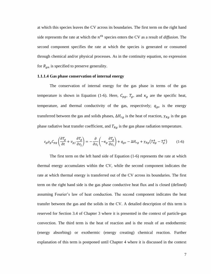
1.1.1.4 Gas phase conservation of internal energy ................................................. 7

1.1.1.5 Gas phase equations of state ....................................................................... 8

1.1.2 Solids phase mathematical model ...................................................................... 8

1.1.2.1 Particle-particle collision model ................................................................. 9

1.1.2.2 Particle-wall collision model .................................................................... 12

1.1.2.3 Gas-solids momentum transfer ................................................................. 13

1.2 Dissertation objectives ............................................................................................ 14

1.3 Document organization ........................................................................................... 15

Chapter 2 : Discrete mass boundary conditions ......................................................... 16 2.1 Introduction ............................................................................................................. 16

2.2 DMIBC algorithm description ................................................................................ 18

2.2.1 DMIBC initialization ....................................................................................... 18

2.2.2 DMIBC operation ............................................................................................ 25

2.3 DMOBC algorithm description .............................................................................. 27

2.4 Implementation ....................................................................................................... 28

2.5 Examples ................................................................................................................. 32

2.5.1 Solids injected into a packed bed ..................................................................... 33

2.5.2 Solids injection coupled with a gas jet ............................................................. 35

2.6 Conclusions ............................................................................................................. 37

Chapter 3 : Particle heat transfer ................................................................................. 38 3.1 Foundations for particle heat transfer ..................................................................... 38

3.1.1 Modes of heat transfer ..................................................................................... 39

3.1.2 Assumption of isothermal particles ................................................................. 40

3.1.3 Particle internal energy equation ..................................................................... 44

3.2 Contact conduction ................................................................................................. 44

3.2.1 Survey of particle-particle contact conduction models .................................... 45

3.2.1.1 Sun and Chen [49] (1988) ......................................................................... 45

v

3.2.1.2 Shimizu [51] (2006) .................................................................................. 49

3.2.1.3 Batchelor and O’Brien [52] (1977) ........................................................... 53

3.2.2 Modified Batchelor and O’Brien [52] two-particle contact conduction model 55

3.2.3 Extension to multi-particle systems ................................................................. 56

3.3 Particle-fluid-particle conduction ........................................................................... 58

3.3.1 Survey of particle-fluid-particle conduction models ....................................... 58

3.3.1.1 Wen and Chang [63] (1967) ..................................................................... 58

3.3.1.2 Delvosalle and Vanderschuren [64] (1985) .............................................. 59

3.3.1.3 Cheng, Yu, and Zulli [65] (1999) ............................................................. 62

3.3.1.4 Rong and Horio [16] (1999) ..................................................................... 65

3.3.2 Modified Rong and Horio [16] particle-fluid-particle conduction model ....... 67

3.4 Particle-gas convection ........................................................................................... 70

3.4.1 Background of particle-gas convection ........................................................... 70

3.4.2 Ranz and Marshall [69] (1952) ........................................................................ 72

3.5 Particle-particle radiation ........................................................................................ 74

3.5.1 Background of particle-particle radiation ........................................................ 75

3.5.2 Environment temperature definition ................................................................ 77

3.6 Implementation of models ...................................................................................... 79

3.6.1 Gas-solids thermal energy transfer .................................................................. 84

3.6.2 Nusselt number correlations ............................................................................ 88

3.6.3 Temperature updating procedures .................................................................... 88

3.6.4 Integral management in particle-fluid-particle conduction model ................... 89

3.7 Verification of implementation ............................................................................... 89

3.7.1 Contact conduction .......................................................................................... 90

3.7.2 Particle-fluid-particle conduction .................................................................... 93

3.7.3 Particle-gas convection .................................................................................... 98

3.7.4 Particle-particle radiation ............................................................................... 101

3.8 Closing Remarks ................................................................................................... 104

Chapter 4 : Particle-gas reactive chemistry interface ............................................... 106 4.1 Foundations for particle-gas reactive chemistry ................................................... 106

4.1.1 Reaction rate .................................................................................................. 107

4.1.2 Specific Heat .................................................................................................. 108

4.1.3 Heat of reaction .............................................................................................. 109

4.1.4 Mass and species equations for a particle ...................................................... 111

4.2 Particle reaction models ........................................................................................ 112

4.2.1 Progressive-conversion model ....................................................................... 112

4.2.2 Shrinking particle model ................................................................................ 113

4.2.3 Shrinking, unreacted-core model ................................................................... 115

4.3 Implementation of interface .................................................................................. 119

4.3.1 Gas-solids mass and species mass transfer .................................................... 124

4.3.2 Mass, species mass, and core radius updating procedures ............................. 125

4.3.3 Specific heat calculations ............................................................................... 126

4.3.4 Heat of reaction calculations .......................................................................... 127

4.3.5 Distribution of the heat of reaction ................................................................ 128

4.3.6 Unreacted core density ................................................................................... 130

4.4 Verification of implementation ............................................................................. 130

vi

4.5 Closing Remarks ................................................................................................... 138

Chapter 5 : Summary and recommendations ............................................................ 139 5.1 Summary of results ............................................................................................... 139

5.1.1 Discrete mass boundary conditions ............................................................... 139

5.1.2 Particle heat transfer ...................................................................................... 139

5.1.3 Particle-gas reactive chemistry interface ....................................................... 141

5.2 Recommendations for future work ....................................................................... 142

Bibliography .................................................................................................................. 145

Appendix A : Geometric definitions for collision calculations ................................. 156

Appendix B : Geometric definitions for conduction models ..................................... 159 B.1 Contact conduction definitions ............................................................................ 159

B.2 Particle-fluid-particle conduction definitions ...................................................... 161

Appendix C : Discrete mass inflow boundary condition source code ...................... 163 C.1 Module - DES_BC ............................................................................................... 163

C.2 : Routine - CHECK_DES_BC ............................................................................. 166

C.3 : Routine - DES_CHECK_MIO_LOCATION .................................................... 172

C.4 : Routine - ALLOCATE_DES_MIO ................................................................... 176

C.5 : Routine - DES_INIT_BC ................................................................................... 178

C.6 : Routine - DES_MI_CLASSIFY ........................................................................ 182

C.7 : Routine - DES_BC_VEL_ASSIGN ................................................................... 188

C.8 : Routine - DES_MI_LAYOUT ........................................................................... 192

C.9 : Routine - DES_MI_CELS ................................................................................. 197

C.10 : Routine - DES_MO_CLASSIFY ..................................................................... 199

C.11 : Routine - DES_MIO_PERIODIC .................................................................... 202

C.12 : Routine - DES_MASS_INLET ........................................................................ 205

C.13 : Routine - DES_PLACE_NEW_PARTICLE ................................................... 210

C.14 : Routine - DES_NEW_PARTICLE_TEST ...................................................... 219

C.15 : Routine - DES_CHECK_PARTICLE ............................................................. 221

C.16 : Routine - DES_MASS_OUTLET .................................................................... 225

Appendix D : Particle heat transfer model source code ............................................ 227 D.1 Module – DES_IC ................................................................................................ 227

D.2 Routine – CHECK_DES_IC ................................................................................ 228

D.3 Routine – DES_SET_IC ...................................................................................... 231

D.4 Module – DES_THERMO ................................................................................... 235

D.5 Routine – CHECK_DES_THERMO ................................................................... 237

D.6 Routine – CALC_THERMO_DES ...................................................................... 242

D.7 Routine – DES_CONDUCTION ......................................................................... 244

D.8 Routine – DES_CONVECTION ......................................................................... 250

D.9 Routine – DES_Hgm ........................................................................................... 252

D.10 Routine –DES_CALC_GAMMA ...................................................................... 254

D.11 Routine –DES_RADIATION ............................................................................ 256

D.12 Routine –DES_THERMO_NEWVALUES ....................................................... 257

D.13 Routine –THERMO_NBR ................................................................................. 259

D.14 Module –INTERPOLATE_CC .......................................................................... 260

vii

D.15 Module –SET_INTERPOLATION_STENCIL_CC ......................................... 262

Appendix E : Interface for managing reactive chemistry source code .................... 266 E.1 Module – DES_RXNS ......................................................................................... 266

E.2 Routine – CHECK_DES_RXNS .......................................................................... 268

E.3 Function – DES_CALC_H ................................................................................... 271

E.4 Routine – DES_PHYSICAL_PROP .................................................................... 272

E.5 Routine – DES_RRATES .................................................................................... 274

E.6 Routine – DES_REACTION_MODEL ............................................................... 281

viii

List of Figures

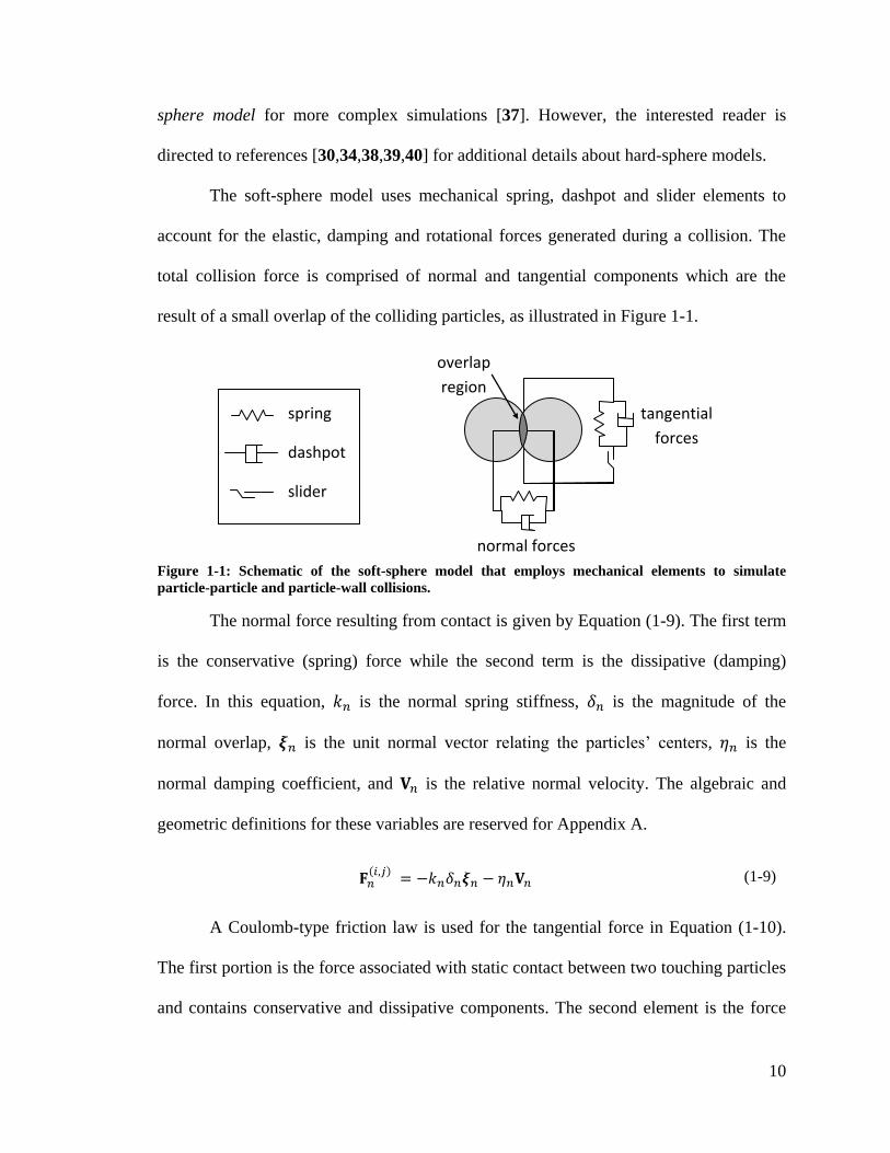
Figure 1-1: Schematic of the soft-sphere model that employs mechanical elements to

simulate particle-particle and particle-wall collisions. ..................................................... 10

Figure 1-2: (a) During a particle-wall collision, an artificial particle the same size of the

colliding particle is generated to represent the wall. The artificial particle is placed

opposite the colliding particle, outside the computational domain. (b) As the position and

trajectory of the colliding particle change, the artificial particles are replaced by new

artificial particles to ensure that normal forces remain normal to the boundary plane. .... 13

Figure 2-1: The staging area for incoming particles is located outside of the

computational domain, in the ghost cells bordering the region identified with the

boundary condition. .......................................................................................................... 17

Figure 2-2: Example distribution array with ten elements, three mass solids phase indices

( , , ) with the respective distribution (20%, 30%, 50%). The fifth array element is

randomly selected, leading to the incoming particle being assigned the properties

associated with solids phase- . .......................................................................................... 19

Figure 2-3: Motivation for a uniform inlet velocity. A slow moving particle is seeded

behind a fast moving particle generating an artificial overlap. ......................................... 21

Figure 2-4: Illustration of the seeding process of the grid structure. In this example, the

sub-grid in the staging area contains seven cells, while two particles are placed every

solids time step. Therefore, the sub-grid will overfill in four solids time steps (eight

particles and only seven cells) if incoming particles do not move with sufficient speed

toward the domain leaving available cells for new particles. ........................................... 24

Figure 2-5: Call graph of main MFIX source code to initialization routines for the

discrete particle model. Dashed lines indicate new calls and subroutines implemented for

the discrete mass boundary conditions. ............................................................................ 30

Figure 2-6: Call graph of MFIX discrete particle model routines. Dashed lines indicate

new calls and subroutines implemented for the discrete mass boundary conditions. ....... 31

Figure 2-7: Flow chart illustrating the locations within MFIX-DEM where modifications

have been made to include discrete mass boundary condition routines. .......................... 32

Figure 2-8: Time series (in seconds) of particle flow for a 2D example illustrating a

DMIBC injecting into a packed bed. ................................................................................ 34

Figure 2-9: Cumulative incoming particle distributions at times 0.5, 3.0, and 5.0 seconds

during the simulation of a DMIBC into a packed particle bed. ........................................ 35

Figure 2-10: Time series (in seconds) of particle flow for a 2D example illustrating a

DMIBC with a gas jet. ...................................................................................................... 36

ix

Figure 3-1: Illustration of conduction between particles. (a) Contact conduction: thermal

energy is transferred from a hot particle to a cold particle through their shared contact

area. (b) Particle-fluid-particle conduction: thermal energy is transferred from a hot

particle to the stagnant gas separating its surface from the cold particle. The thermal

energy is then transferred from the stagnant gas to the cold particle. ............................... 39

Figure 3-2: Illustration of particle-gas convection. Thermal energy is exchanged between

the surface of the particle and the moving fluid. .............................................................. 40

Figure 3-3: Illustration of particle-environment radiative heat transfer. Electromagnetic

waves transmitted by a hot particle are absorbed and reflected by the cold particle. ....... 40

Figure 3-4: Illustration of Biot number classification on a particle’s temperature. Arrows

on the surface of the particles indicate the rate of convective heat transfer, while the

arrows inside the particle represent the rate of conductive heat transfer. (a) For small Biot

numbers, a particle’s temperature is nearly-isothermal because the redistribution of

thermal energy within a particle occurs at a faster rate than convective heat transfer. (b)

When the Biot number is large, a temperature gradient may exist within a particle

because the redistribution of thermal energy inside a particle is slower than the rate of

convective heat transfer. ................................................................................................... 43

Figure 3-5: The elastic collision model employed by Sun and Chen [49] leads to the

assumption that the shared contact area is flat. ................................................................. 46

Figure 3-6: Particle-particle conduction model employing a thermal pipe connecting the

centers of two particles. Implemented in PFC2D/3D [56,57] and presented by Shimizu

[51]. ................................................................................................................................... 50

Figure 3-7: Illustration of a particle assembly as defined by Shimizu [51] with

interconnected thermal pipes. ........................................................................................... 51

Figure 3-8: Illustration of the thermal energy flux from a hot particle to a cold particle

across the contact area. ..................................................................................................... 54

Figure 3-9: Illustration depicting the heat transfer paths as defined by Delvosalle and

Vanderschuren’s [64]. The heat transfer paths are defined as portions of circumferences

perpendicular to the surfaces of the particles. ................................................................... 60

Figure 3-10: Delvosalle and Vanderschuren’s [64] model assumes particle-fluid-particle

conduction is initiated when the laminar sub-layers surrounding two particles overlap.

This configuration is used to define the parameter in Equation (3-42). ........................ 61

Figure 3-11: The model of Cheng, Yu, and Zulli [65] restricts particle-fluid-particle

conduction to the region delineated by the double pyramid (3-D) generated by the

Voronoi-boundary plane. .................................................................................................. 62

x

Figure 3-12: Cheng, Yu, and Zulli’s [65] Model A for particle-fluid-particle conduction

assumes that the surface of the double tapered cone is isothermal, conduction is

negligible in the outer region of the double tapered cone, and the heat transfer paths are

parallel to the axis joining the particles’ centers. .............................................................. 63

Figure 3-13: Geometric representation of quantities used by Cheng, Yu, and Zulli’s [65]

Model A for particle-fluid-particle conduction. ................................................................ 63

Figure 3-14: Cheng, Yu, and Zulli’s [65] Model B for particle-fluid-particle conduction

assumes that each particle has an isothermal core and the paths of heat transfer radiate

from the particles centers. ................................................................................................. 64

Figure 3-15: Rong and Horio’s [16] configuration for particle-fluid-particle conduction.

In their model, each particle is surrounded by a gas layer and heat transfer occurs across

paths parallel to the line connecting the centers of the particles. When particles engage in

contact, the overlap region is assumed to have a uniform gas layer separating the

particles’ surfaces. ............................................................................................................. 66

Figure 3-16: Illustration of geometric quantities delineating the region of particle fluid

heat transfer imposed in this work. ................................................................................... 68

Figure 3-17: A singularly arises in the modified Rong and Horio model at the interface of

the contact boundary. This is corrected by prohibiting perfect contact between particles,

and require a minimum separation distance of . Similar assumptions are

employed by Delvosalle and Vanderschuren [64] and Rong and Horio [16]. .................. 69

Figure 3-18: A multi-particle radiation problem is reduced by assuming that the particles

predominantly exposed to radiation form a spherical environment surrounding the

particle of interest. ............................................................................................................ 76

Figure 3-19: Illustration of the sub-domain model proposed by Zhou, Yu, and Zulli [19]

for determining the environment temperature used to calculate the rate of radiative heat

transfer with particle . In this example, three particles are in the sub-domain (i.e.,

) of particle . ................................................................................................... 78

Figure 3-20: Call graph of main MFIX-DEM source code for initialization routines.

Dashed lines indicate new calls and subroutines implemented for the heat transfer model.

........................................................................................................................................... 81


new calls and subroutines implemented for the heat transfer model. ............................... 82


have been made to include particle heat transfer. ............................................................. 83

Figure 3-23: Flow chart illustrating customizability of the implementation by allowing a

user to select which modes of heat transfer to compute during a simulation. ................. 84

xi

Figure 3-24: Example illustrating the Eulerian grid which stores scalar field variables,

like temperature, at the cell-center. Particles are permitted to exist at any location within

the domain defined by the Eulerian grid. .......................................................................... 85

Figure 3-25: Example illustrating the two methods available to transmitting thermal

energy between the Eulerian grid and the particles. (a) Energy is passed between a

particle and the grid cell containing its center; (b) energy is distributed from a particle’s

position to the nearest grid cells........................................................................................ 86

Figure 3-26: Illustration of the fluid step forward-particle catch-up process that occurs

during MFIX-DEM. First the solution to the fluid phase if obtained at time , then

multiple, smaller time steps are taken within the DEM to allow the particles to catch-up

to the fluid phase. Here, is the time of the fluid’s most recent solution, and is the time

of the discrete solids most recent solution. ....................................................................... 87

Figure 3-27: The geometric configuration of the particles used to verify the

implementation of the contact conduction model implemented into MFIX-DEM. All

measurements are in centimeters. ..................................................................................... 92

Figure 3-28: MFIX-DEM and analytic solutions to the internal energy equation for two

particles engaged in contact conduction. Tp1 and Tp2 are the temperatures of the cold

and hot particles, respectively. Relative error between the analytic and numerical

solutions is indicated by open symbols and is associated with the right vertical axis. ..... 93

Figure 3-29: The geometric configuration of the particles used in the first simulation to

verify the implementation of the particle-fluid-particle conduction model implemented

into MFIX-DEM. All measurements are in centimeters. .................................................. 96


particles not touching and engaged in particle-fluid-particle conduction. Tp1 and Tp2 are

the temperatures of particle 1 and particle 2, respectively (c.f. Table 3-4). Relative error

between the two solutions is indicated by open symbols and is associated with the right

vertical axis. ...................................................................................................................... 97


touching particles engaged in particle-fluid-particle conduction. Tp1 and Tp2 are the

temperatures of particle 1 and particle 2, respectively (c.f. Table 3-4). Relative error

between the two solutions is indicated by open symbols and is associated with the right

vertical axis. ...................................................................................................................... 97

Figure 3-32: The geometric configuration of a particle used to verify the implementation

of the particle-gas convection model implemented into MFIX-DEM. All measurements

are in centimeters. ............................................................................................................. 99

xii

Figure 3-33: MFIX-DEM and analytic solutions to the internal energy equation for a

single particle undergoing particle-gas convection with a constant fluid. Tp and Tg are

the temperatures of particle and gas, respectively Relative error between the numerical

and analytic solutions is indicated by open symbols and is associated with the right

vertical axis. .................................................................................................................... 100

Figure 3-34: The geometric configuration of the particles used in the first simulation to

verify the implementation of the particle-environment radiation model implemented into

MFIX-DEM. All measurements are in centimeters. ....................................................... 103

Figure 3-35: MFIX-DEM and fourth order Runge-Kutta (RK4) solutions to the internal

energy equation for two particles not touching engaged in radiative heat exchange.

Relative error between the two solutions is indicated by open symbols and is associated

with the right vertical axis. .............................................................................................. 104

Figure 4-1: Illustration of the progressive-conversion model. The reaction occurs

uniformly throughout a particle, leaving the particle size unchanged. In this example, the

concentration of the reactant diminishes as the reaction proceeds. ................................ 112

Figure 4-2: Illustration of the shrinking particle model. The reaction occurs at the

particle’s surface while the composition of the particle does not change. Any solid

products of the reaction are assumed to ‘flake off’ of the particle’s surface (i.e. no solid

products collect on the surface of the particle). .............................................................. 114

Figure 4-3: An example illustrating how the number of possible neighbor particles

increases as the ratio of the neighbor’s radius ( ) to the particle’s radius ( )

decreases. ........................................................................................................................ 115

Figure 4-4: Illustration of the shrinking core model. The reaction occurs at the surface of

the particle’s unreacted core with an inert solid (ash) replacing the particle’s solids.

Although the unreacted core shrinks as the reaction proceeds, its composition remains

constant. .......................................................................................................................... 116

Figure 4-5: Example illustrating the connection between the radius of the unreacted core

( ) and the definition of the unreacted core’s density ( ). If the unreacted core’s

density ( ) is equated to the particle’s initial density ( ), then the core’s radius

shrinks to . If the unreacted core’s density is defined as the initial mass of the solid

phase reactants divided by the particle’s volume ( ), the core’s radius

shrinks to . Finally, if the unreacted core’s density is defined as the total mass of solid

phase reactants consumed divided by particle’s volume ( ), then the

core’s radius shrinks to zero. .......................................................................................... 117

Figure 4-6: Call graph of main MFIX-DEM source code for initialization routines.

Dashed lines indicate new calls and subroutines implemented for the reactive chemistry

interface. .......................................................................................................................... 121

xiii


new calls and subroutines implemented for the reactive chemistry interface. ............... 122


have been made to include the reactive chemistry interface. .......................................... 123

Figure 4-9: MFIX-DEM and analytic solutions to the particle mass equation engaged in

reactive chemistry interface. mp is the mass of the particle. Relative error between the

analytic and numerical (forward Euler method) solutions is indicated by open symbols

and is associated with the right vertical axis. .................................................................. 135

Figure 4-10: MFIX-DEM and analytic solutions to the particle species equations engaged

in reactive chemistry interface. XB, XD, and XI are the species mass fractions for species

B, D, and I, respectively. Absolute error between the analytic and numerical (forward

Euler method) solutions is indicated by open symbols and is associated with the right

vertical axis. .................................................................................................................... 136

Figure 4-11: MFIX-DEM and analytic solutions to the particle energy equation engaged

in reactive chemistry interface. Tp is the temperature of the particle. Relative error

between the analytic and numerical (forward Euler method) solutions is indicated by

open symbols and is associated with the right vertical axis. ........................................... 136

Figure 4-12: MFIX-DEM and analytic solutions to the radius of the shrinking, unreacted

core engaged in reactive chemistry interface. Rc is the core radius. Absolute error

between the analytic and numerical (forward Euler and Adams-Bashforth (AB) methods)

solutions are indicated by open symbols and is associated with the right vertical axis. . 137

Figure A-1: Schematic demonstrating various terms needed in the calculation of the

particle-particle collision force. ...................................................................................... 156

Figure B-1: Schematic demonstrating various terms needed in the calculation of the

contact radius needed for computing contact conduction. In this illustration particle is

smaller than particle . .................................................................................................... 159








particle-fluid-particle conduction. ................................................................................... 161

xiv

List of Tables

Table 2-1: A list of the subroutines comprising the discrete mass boundary conditions

with brief description of their use. .................................................................................... 28

Table 2-2: Particle and feed properties of the examples outlined in Sections 2.5.1 and

2.5.2................................................................................................................................... 33

Table 3-1: Summary of the particle internal energy equation and four forms of particle

heat transfer considered in this work. ............................................................................... 79

Table 3-2: A list of subroutines developed to set initial conditions of particles and

manage the heat transfer models implemented into MFIX. .............................................. 80

Table 3-3: Physical and thermodynamic properties of the particles used to verify the

contact conduction model implemented into MFIX-DEM. The geometric configuration is

illustrated in Figure 3-27. .................................................................................................. 91


particle-fluid-particle conduction model implemented into MFIX-DEM. The geometric

configuration for the first simulation is illustrated in Figure 3-29 while the geometric

configuration for the second simulation is illustrated in Figure 3-27. The gas phase

thermal conductivity for both simulations was set as 1.239x10-4

cal/sec·cm·K. .............. 95

Table 3-5: Physical and thermodynamic properties of the gas and particle used to verify

the convection model implemented into MFIX-DEM. The geometric configuration is

illustrated in Figure 3-32. .................................................................................................. 99


radiative heat transfer model implemented into MFIX-DEM. The geometric configuration

is illustrated in Figure 3-34. ............................................................................................ 102

Table 4-1: Summary of the models managed by the reactive chemistry interface

considered in this work. .................................................................................................. 120

Table 4-2: A list of subroutines developed for the reactive chemistry interface

implemented into MFIX. ................................................................................................ 120

Table 4-3: Physical and thermodynamic properties of the gas and particle used to verify

the reactive chemistry interface implemented into MFIX-DEM. ................................... 134

Table 4-4: Physical and thermodynamic properties of the gas and particle species used to

verify the reactive chemistry interface implemented into MFIX-DEM. ........................ 134

xv

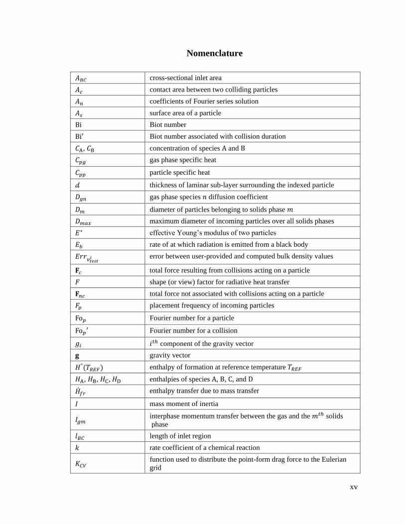
Nomenclature

cross-sectional inlet area

contact area between two colliding particles

coefficients of Fourier series solution

surface area of a particle

Biot number

Biot number associated with collision duration

, concentration of species and

gas phase specific heat

particle specific heat

thickness of laminar sub-layer surrounding the indexed particle

gas phase species diffusion coefficient

diameter of particles belonging to solids phase

maximum diameter of incoming particles over all solids phases

effective Young’s modulus of two particles

rate of at which radiation is emitted from a black body

error between user-provided and computed bulk density values

total force resulting from collisions acting on a particle

shape (or view) factor for radiative heat transfer

total force not associated with collisions acting on a particle

placement frequency of incoming particles

Fourier number for a particle

Fourier number for a collision

component of the gravity vector

gravity vector

enthalpy of formation at reference temperature

, , , enthalpies of species , , , and

enthalpy transfer due to mass transfer

mass moment of inertia

interphase momentum transfer between the gas and the solids

phase

length of inlet region

rate coefficient of a chemical reaction

function used to distribute the point-form drag force to the Eulerian

grid

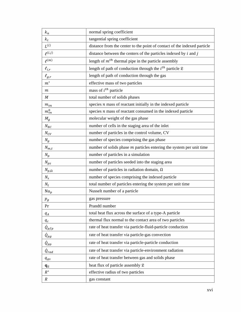
xvi

normal spring coefficient

tangential spring coefficient

distance from the center to the point of contact of the indexed particle

distance between the centers of the particles indexed by and

length of thermal pipe in the particle assembly

length of path of conduction through the particle

length of path of conduction through the gas

effective mass of two particles

mass of particle

total number of solids phases

species mass of reactant initially in the indexed particle

species mass of reactant consumed in the indexed particle

molecular weight of the gas phase

number of cells in the staging area of the inlet

number of particles in the control volume, CV

number of species comprising the gas phase

number of solids phase particles entering the system per unit time

number of particles in a simulation

number of particles seeded into the staging area

number of particles in radiation domain,

number of species comprising the indexed particle

total number of particles entering the system per unit time

Nusselt number of a particle

gas pressure

Prandtl number

total heat flux across the surface of a type-A particle

thermal flux normal to the contact area of two particles

rate of heat transfer via particle-fluid-particle conduction

rate of heat transfer via particle-gas convection

rate of heat transfer via particle-particle conduction

rate of heat transfer via particle-environment radiation

rate of heat transfer between gas and solids phase

heat flux of particle assembly

effective radius of two particles

gas constant

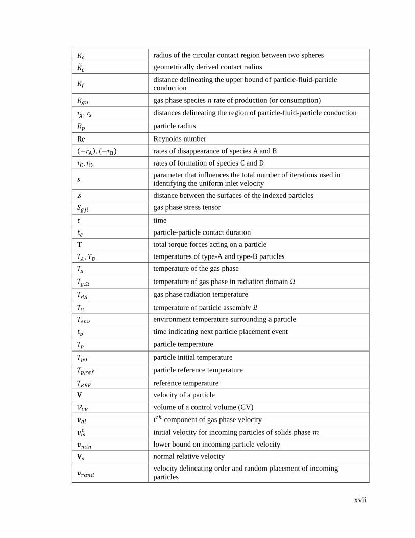
xvii

radius of the circular contact region between two spheres

geometrically derived contact radius

distance delineating the upper bound of particle-fluid-particle

conduction

gas phase species rate of production (or consumption)

, distances delineating the region of particle-fluid-particle conduction

particle radius

Reynolds number

rates of disappearance of species and

rates of formation of species and

parameter that influences the total number of iterations used in

identifying the uniform inlet velocity

distance between the surfaces of the indexed particles

gas phase stress tensor

time

particle-particle contact duration

total torque forces acting on a particle

, temperatures of type-A and type-B particles

temperature of the gas phase

temperature of gas phase in radiation domain

gas phase radiation temperature

temperature of particle assembly

environment temperature surrounding a particle

time indicating next particle placement event

particle temperature

particle initial temperature

particle reference temperature

reference temperature

velocity of a particle

volume of a control volume (CV)

component of gas phase velocity

initial velocity for incoming particles of solids phase

lower bound on incoming particle velocity

normal relative velocity

velocity delineating order and random placement of incoming

particles

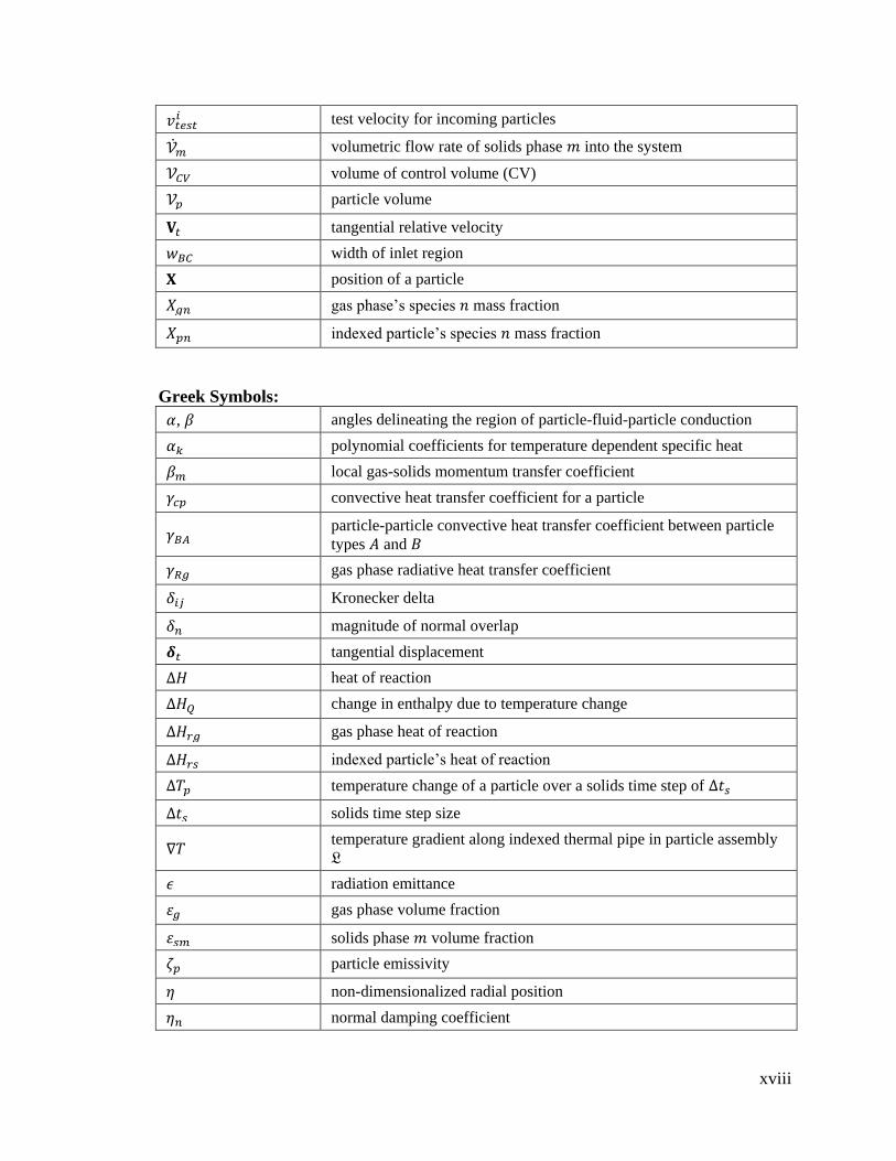
xviii

test velocity for incoming particles

volumetric flow rate of solids phase into the system

volume of control volume (CV)

particle volume

tangential relative velocity

width of inlet region

position of a particle

gas phase’s species mass fraction

indexed particle’s species mass fraction

Greek Symbols:

, angles delineating the region of particle-fluid-particle conduction

polynomial coefficients for temperature dependent specific heat

local gas-solids momentum transfer coefficient

convective heat transfer coefficient for a particle

particle-particle convective heat transfer coefficient between particle

types and

gas phase radiative heat transfer coefficient

Kronecker delta

magnitude of normal overlap

tangential displacement

heat of reaction

change in enthalpy due to temperature change

gas phase heat of reaction

indexed particle’s heat of reaction

temperature change of a particle over a solids time step of

solids time step size

temperature gradient along indexed thermal pipe in particle assembly

radiation emittance

gas phase volume fraction

solids phase volume fraction

particle emissivity

non-dimensionalized radial position

normal damping coefficient

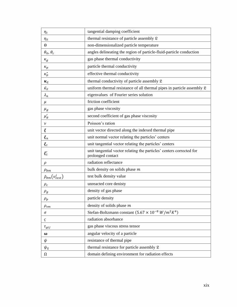
xix

tangential damping coefficient

thermal resistance of particle assembly

non-dimensionalized particle temperature

, angles delineating the region of particle-fluid-particle conduction

gas phase thermal conductivity

particle thermal conductivity

effective thermal conductivity

thermal conductivity of particle assembly

uniform thermal resistance of all thermal pipes in particle assembly

eigenvalues of Fourier series solution

friction coefficient

gas phase viscosity

second coefficient of gas phase viscosity

Poisson’s ration

unit vector directed along the indexed thermal pipe

unit normal vector relating the particles’ centers

unit tangential vector relating the particles’ centers

unit tangential vector relating the particles’ centers corrected for

prolonged contact

radiation reflectance

bulk density on solids phase

test bulk density value

unreacted core denisty

density of gas phase

particle density

density of solids phase

Stefan-Boltzmann constant

radiation absorbance

gas phase viscous stress tensor

angular velocity of a particle

resistance of thermal pipe

thermal resistance for particle assembly

domain defining environment for radiation effects

xx

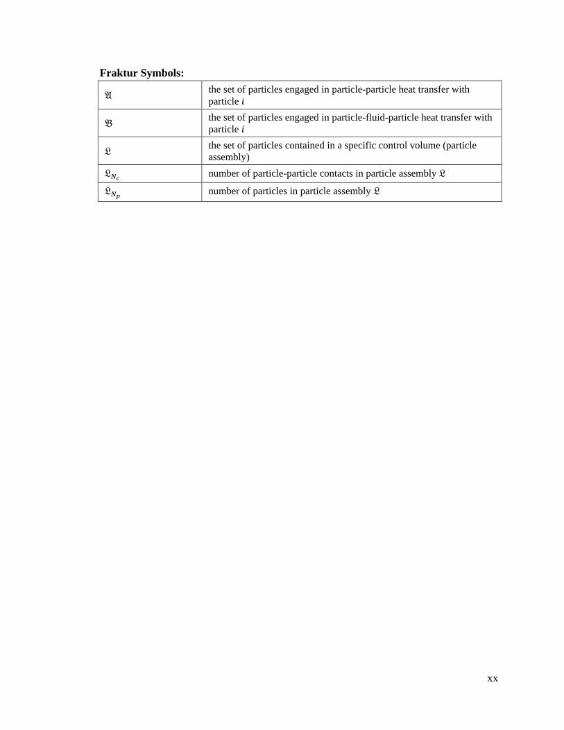
Fraktur Symbols:

the set of particles engaged in particle-particle heat transfer with

particle

the set of particles engaged in particle-fluid-particle heat transfer with

particle

the set of particles contained in a specific control volume (particle

assembly)

number of particle-particle contacts in particle assembly

number of particles in particle assembly

xxi

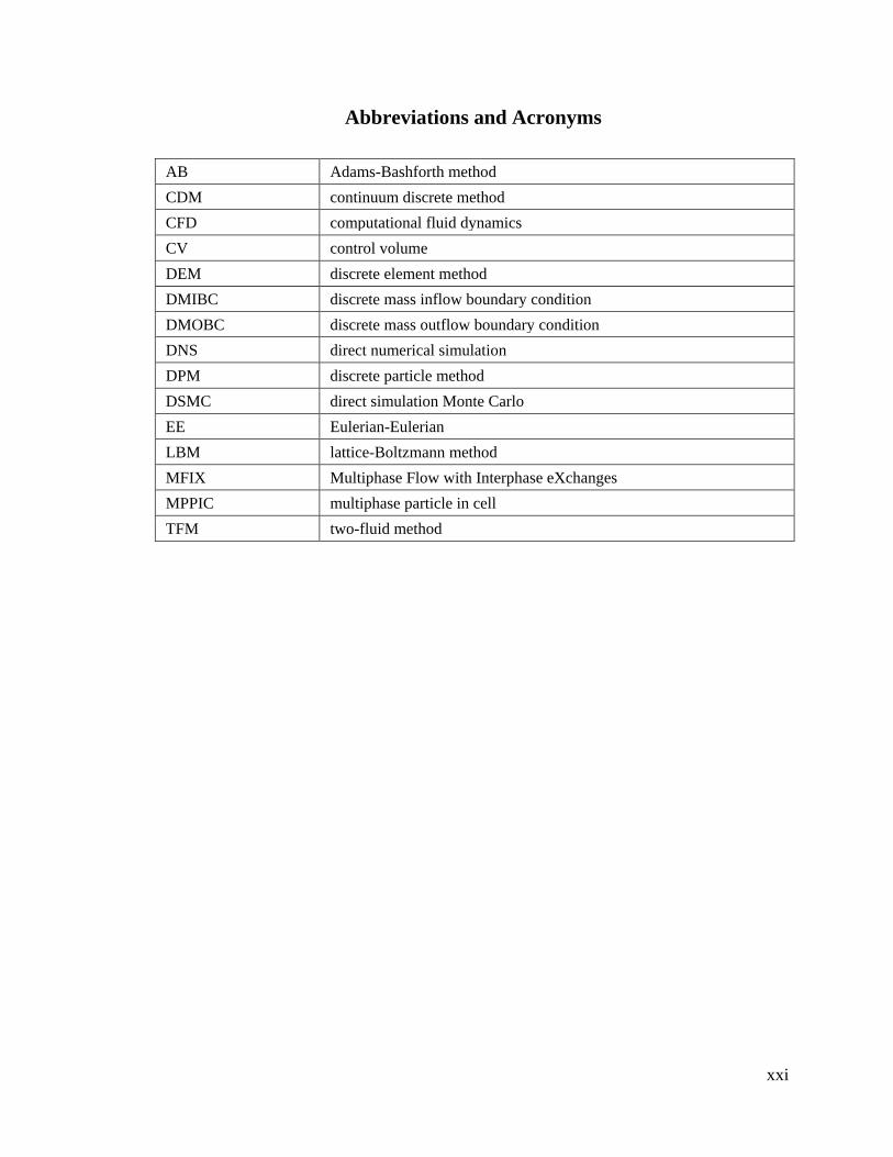
Abbreviations and Acronyms

AB Adams-Bashforth method

CDM continuum discrete method

CFD computational fluid dynamics

CV control volume

DEM discrete element method

DMIBC discrete mass inflow boundary condition

DMOBC discrete mass outflow boundary condition

DNS direct numerical simulation

DPM discrete particle method

DSMC direct simulation Monte Carlo

EE Eulerian-Eulerian

LBM lattice-Boltzmann method

MFIX Multiphase Flow with Interphase eXchanges

MPPIC multiphase particle in cell

TFM two-fluid method

1

Chapter 1: Introduction

Gas-solids systems are found in industrial food preparation, mineral processing,

pharmaceutical production, energy generation, and chemical production setups as well as

academic research laboratories world-wide. Applications range from co-current flow

drying processes for food particles [1] to fluidized bed reactors for polyethylene

production [2]. With such a large industrial dependence on gas-solids systems, it is

imperative that they are fully understood. A greater understanding of the physical

processes occurring within a gas-solids system may yield designs that are more cost

effective, energy efficient, and environmentally friendly.

Traditionally, design, scaling, and optimization of gas-solids systems are guided

by empirical models derived from experimental observations [3,4]. The development of

these models requires a large investment in both time and capital while their predictive

capabilities remain limited and unreliable [5]. Consequently, multiphase computational

fluid dynamics (CFD) models are gaining in popularity for testing various design

considerations [6] and predicting flow characteristics [7]. This physics-based approach

provides greater modeling flexibility since it is rooted in the first principles of gas-solids

dynamics [8].

There are two general methods for modeling gas-solids flows. Simulations that

solve continuum conservation equations for both the gas and solids phases are termed

Eulerian-Eulerian (EE) or two fluid methods (TFM). Simulations that manage distinct

objects for the solids phase while continuum conservation equations are solved for the

gas phase are called Lagrangian-Eulerian (LE) or continuum discrete methods (CDM).

2

CDMs encompass a wide range of models that resolve gas-solids flow

characteristics at various length and time scales [5]. These techniques include direct

numerical simulation (DNS), lattice-Boltzmann method (LBM), CFD-discrete element

method (CFD-DEM), direct simulation Monte Carlo method (DSMC), and multiphase

particle in cell (MPPIC) methods. Each approach leads to a trade-off between

computational expense and modeling complexity. A brief overview of these methods is

found in the book, Multiphase Continuum Formulation of Gas-Solids Reacting Flows by

Pannala, Syamlal, and O’Brien [5]. The primary goal of this work is to further the

modeling capabilities of an existing CFD-DEM. Section 1.1 provides an overview of this

modeling technique so that the objectives of this work are defined more clearly.

1.1 CFD-Discrete element method (CFD-DEM)

CFD-DEM combines two different modeling techniques for simulating gas-solids

flows. The gas phase is described by a set of conservation equations that are solved over

a static grid, similar to single phase CFD. In contrast, the solids phase is described by a

collection of discrete particles that obey Newton’s laws of motion. Each particle is

individually tracked and all particle-particle collisions are resolved. This method of solids

modeling is termed the discrete element method (DEM) but often is referred to as the

discrete particle method (DPM).

The original concept of the CFD-DEM is found in the pioneering work of Tsuji,

Tanaka, and Ishida [9]. In their research, a simple gas phase model is coupled with a

DEM to simulate plug flow in a horizontal pipe. Since then, the simulation capabilities of

the CFD-DEM have advanced. Initial investigations strived to refine the gas phase model

[10,11], while new developments continue to improve the coupling of the gas and solids

3

phases [12]. Some research groups have incorporated Van der Waals forces to simulate

cohesion between particles [13,14] as well as the Saffman and Magnus lift forces [15].

Presently, there is a large effort to include particle scale heat transfer and reactive

chemistry models [2,11,16,17,18,19,20,21,22,23]. Sections 1.1.1 and 1.1.2 present the

mathematical models for the gas and solids phases employed by the current CFD-DEM.

A brief discussion covering the physical interpretation of the equations' components is

provided. The gas phase model is introduced first, followed by a presentation of the

solids phase model.

1.1.1 Gas phase mathematical model

The gas phase model employed by the CFD-DEM in this work is based on the

volume averaging method of Anderson and Jackson [24,25]. In this approach, continuum

equations for the gas phase are derived from the point form Navier-Stokes equations by

converting point variables (e.g., gas velocity) to local mean variables [8]. The

transformation occurs by incorporating a weighting function when averaging point

variables over a region (volume) in space. Regions are defined so that they are small in

comparison to macroscopic changes in flow characteristics within the system, but large

enough to contain many particles [26].

The governing equations presented below only contain the source and sink terms

found in references [24,25,27]. Constitutive relationships needed to define various terms

that arise during the derivation of the continuum equations (model closure) are obtained

from the gas-solids flow theory outlined by Syamlal, Rogers, and O'Brien [27]. A

complete review of all possible source and sink terms as well as the many constitutive

relationships presented in the literature is beyond the scope of this work.

4

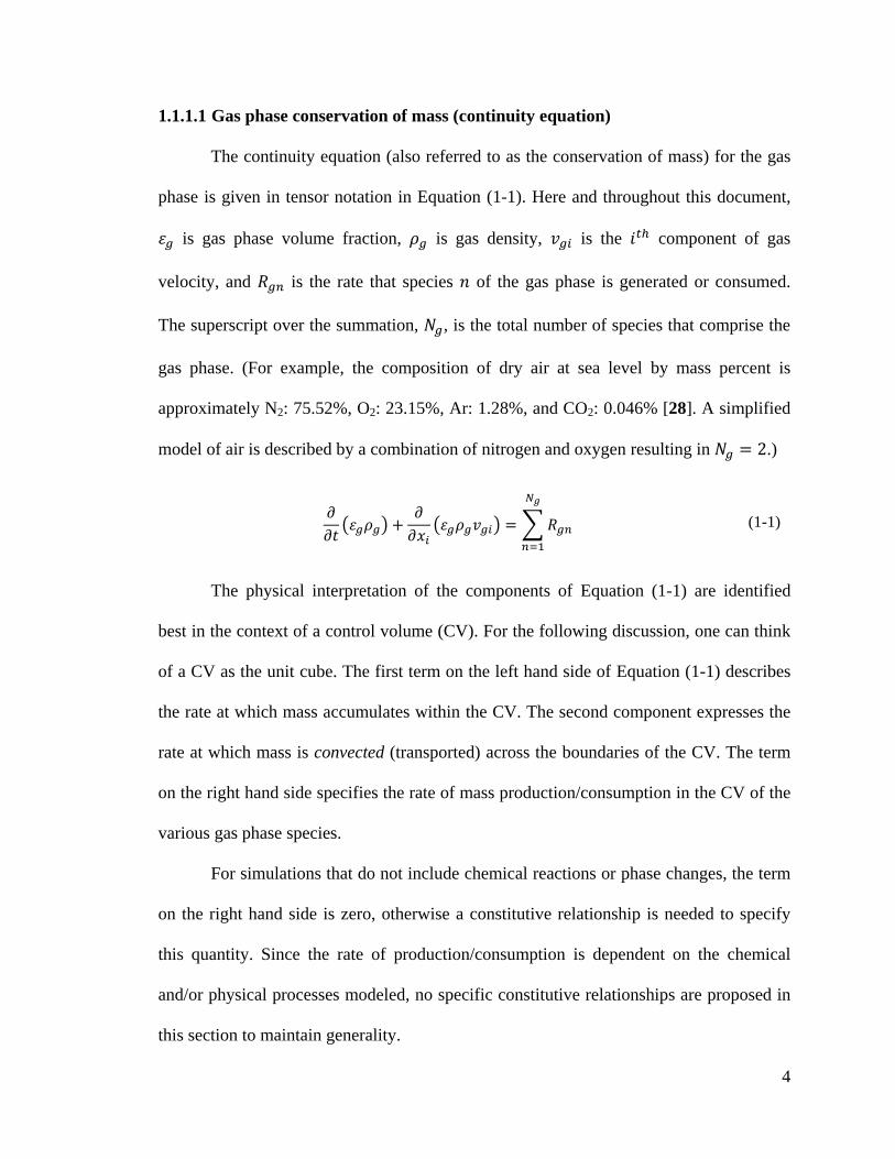
1.1.1.1 Gas phase conservation of mass (continuity equation)

The continuity equation (also referred to as the conservation of mass) for the gas

phase is given in tensor notation in Equation (1-1). Here and throughout this document,

is gas phase volume fraction, is gas density, is the component of gas

velocity, and is the rate that species of the gas phase is generated or consumed.

The superscript over the summation, , is the total number of species that comprise the

gas phase. (For example, the composition of dry air at sea level by mass percent is

approximately N2: 75.52%, O2: 23.15%, Ar: 1.28%, and CO2: 0.046% [28]. A simplified

model of air is described by a combination of nitrogen and oxygen resulting in .)

(1-1)

The physical interpretation of the components of Equation (1-1) are identified

best in the context of a control volume (CV). For the following discussion, one can think

of a CV as the unit cube. The first term on the left hand side of Equation (1-1) describes

the rate at which mass accumulates within the CV. The second component expresses the

rate at which mass is convected (transported) across the boundaries of the CV. The term

on the right hand side specifies the rate of mass production/consumption in the CV of the

various gas phase species.

For simulations that do not include chemical reactions or phase changes, the term

on the right hand side is zero, otherwise a constitutive relationship is needed to specify

this quantity. Since the rate of production/consumption is dependent on the chemical

and/or physical processes modeled, no specific constitutive relationships are proposed in

this section to maintain generality.

5

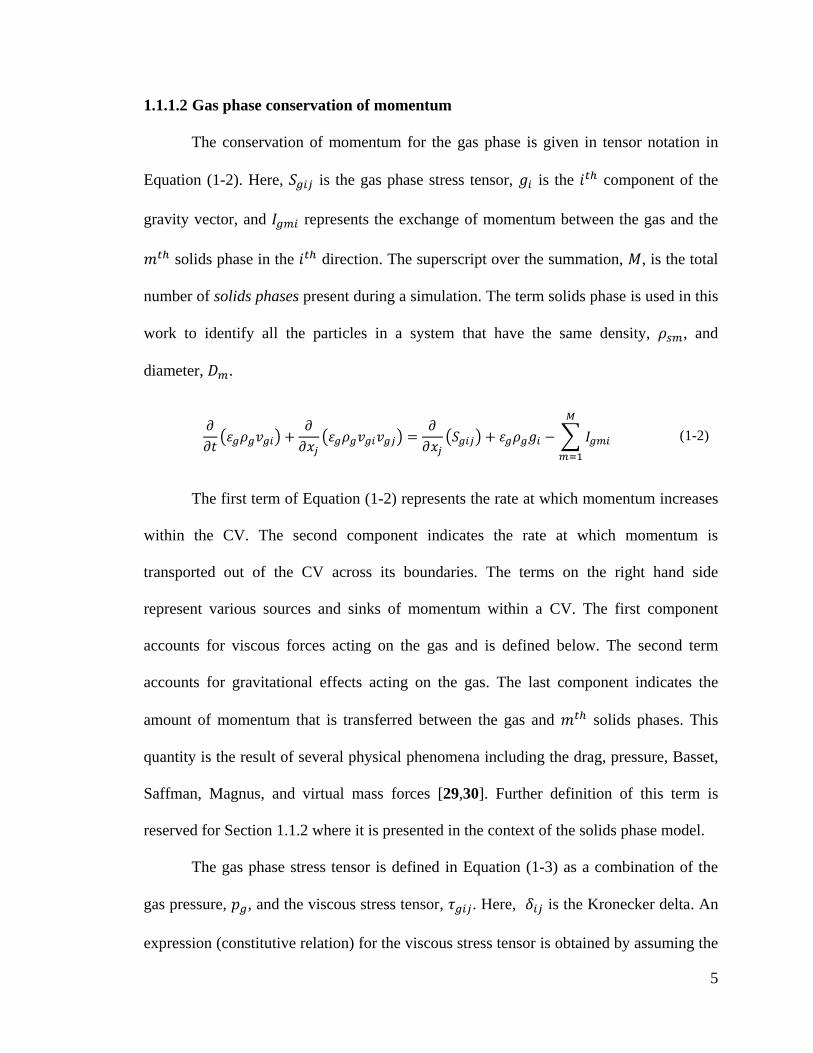
1.1.1.2 Gas phase conservation of momentum

The conservation of momentum for the gas phase is given in tensor notation in

Equation (1-2). Here, is the gas phase stress tensor, is the component of the

gravity vector, and represents the exchange of momentum between the gas and the

solids phase in the direction. The superscript over the summation, , is the total

number of solids phases present during a simulation. The term solids phase is used in this

work to identify all the particles in a system that have the same density, , and

diameter, .

(1-2)

The first term of Equation (1-2) represents the rate at which momentum increases

within the CV. The second component indicates the rate at which momentum is

transported out of the CV across its boundaries. The terms on the right hand side

represent various sources and sinks of momentum within a CV. The first component

accounts for viscous forces acting on the gas and is defined below. The second term

accounts for gravitational effects acting on the gas. The last component indicates the

amount of momentum that is transferred between the gas and solids phases. This

quantity is the result of several physical phenomena including the drag, pressure, Basset,

Saffman, Magnus, and virtual mass forces [29,30]. Further definition of this term is

reserved for Section 1.1.2 where it is presented in the context of the solids phase model.

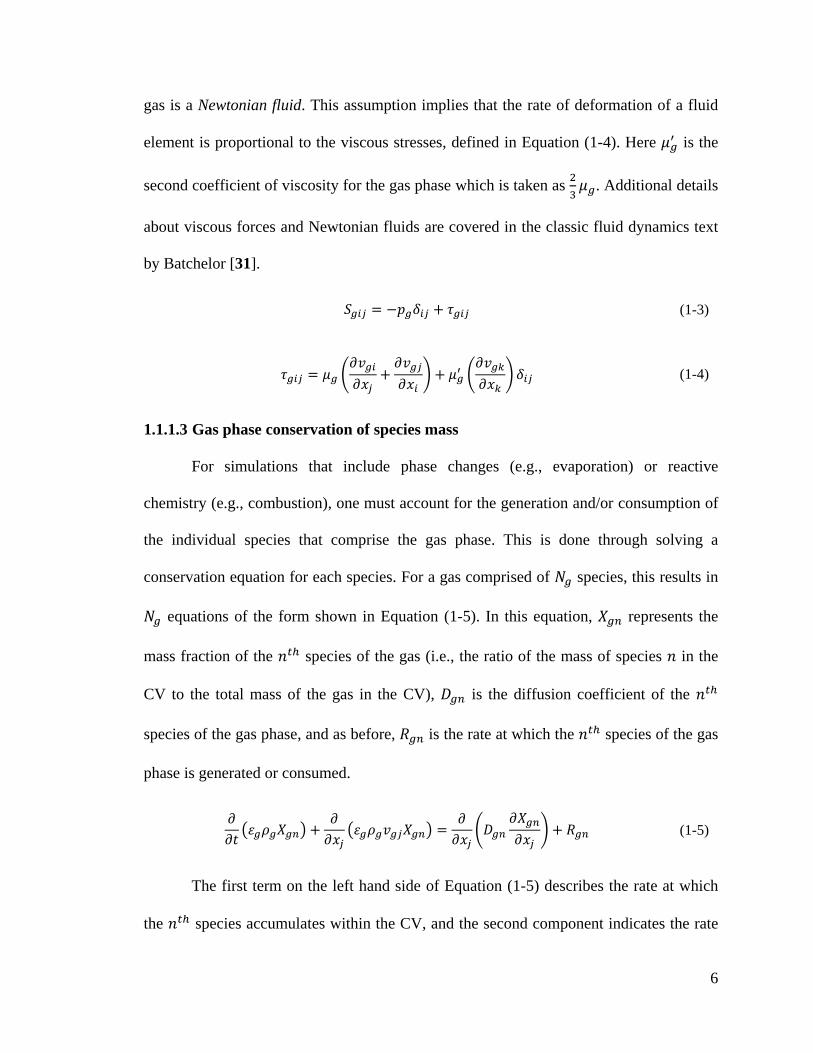
The gas phase stress tensor is defined in Equation (1-3) as a combination of the

gas pressure, , and the viscous stress tensor, . Here, is the Kronecker delta. An

expression (constitutive relation) for the viscous stress tensor is obtained by assuming the

6

gas is a Newtonian fluid. This assumption implies that the rate of deformation of a fluid

element is proportional to the viscous stresses, defined in Equation (1-4). Here is the

second coefficient of viscosity for the gas phase which is taken as

. Additional details

about viscous forces and Newtonian fluids are covered in the classic fluid dynamics text

by Batchelor [31].

(1-3)

(1-4)

1.1.1.3 Gas phase conservation of species mass

For simulations that include phase changes (e.g., evaporation) or reactive

chemistry (e.g., combustion), one must account for the generation and/or consumption of

the individual species that comprise the gas phase. This is done through solving a

conservation equation for each species. For a gas comprised of species, this results in

equations of the form shown in Equation (1-5). In this equation, represents the

mass fraction of the species of the gas (i.e., the ratio of the mass of species in the

CV to the total mass of the gas in the CV), is the diffusion coefficient of the

species of the gas phase, and as before, is the rate at which the species of the gas

phase is generated or consumed.

(1-5)

The first term on the left hand side of Equation (1-5) describes the rate at which

the species accumulates within the CV, and the second component indicates the rate

7

at which this species leaves the CV across its boundaries. The first term on the right hand

side represents the rate at which the species enters the CV as a result of diffusion. The

second component specifies the rate at which the species is generated or consumed

through chemical and/or physical processes. As in the continuity equation, no expression

for is specified to preserve generality.

1.1.1.4 Gas phase conservation of internal energy

The conservation of internal energy for the gas phase in terms of the gas

temperature is shown in Equation (1-6). Here, , , and are the specific heat,

temperature, and thermal conductivity of the gas, respectively; is the energy

transferred between the gas and solids phases, is the heat of reaction, is the gas

phase radiative heat transfer coefficient, and is the gas phase radiation temperature.

(1-6)

The first term on the left hand side of Equation (1-6) represents the rate at which

thermal energy accumulates within the CV, while the second component indicates the

rate at which thermal energy is transferred out of the CV across its boundaries. The first

term on the right hand side is the gas phase conductive heat flux and is closed (defined)

assuming Fourier’s law of heat conduction. The second component indicates the heat

transfer between the gas and the solids in the CV. A detailed description of this term is

reserved for Section 3.4 of Chapter 3 where it is presented in the context of particle-gas

convection. The third term is the heat of reaction and is the result of an endothermic

(energy absorbing) or exothermic (energy creating) chemical reaction. Further

explanation of this term is postponed until Chapter 4 where it is discussed in the context

8

of the mathematical interface for managing gas-solids reactions. The last component is

described via a simplified model for radiative heat transfer in the gas phase.

1.1.1.5 Gas phase equations of state

In addition to the gas phase continuity and internal energy equations, specifying

an equation of state establishes a relationship between the thermodynamic variables of

density, pressure, temperature, and specific internal energy. The ideal gas law, shown in

Equation (1-7), is used commonly in CFD for compressible fluids [32]. In this example,

the density of the gas is defined by the gas constant and the pressure , molecular

weight , and temperature of the gas, respectively. If the gas phase is assumed

incompressible, then it is common to define the density of the gas as a constant value.

(1-7)

This concludes the outline of the equations governing the gas phase. The

interested reader is directed to [29,33] for additional theoretical treatment of gas phase

modeling for multiphase flows.

1.1.2 Solids phase mathematical model

The solids phase in the CFD-DEM is represented by a collection of discrete

particles that obey Newton’s equations of motion, shown in Equation set (1-8). In these

equations, for a particle indexed by the superscript , the variables , , , and

indicate the particle’s mass, position, linear and angular velocities, and mass moment of

inertia, respectively.

are the total forces resulting from particle-particle and particle-

wall collisions,

are the total forces not associated with collisions (i.e., gas-solids

9

interaction, cohesion, etc.) , and is the total torque acting on particle . Bold face font

is used throughout this work to identify vector quantities.

(1-8)

The first equation in set (1-8) defines the velocity of the particle as the time rate

of change of the particle's position. The second equation is typically referred to as

Newton’s Second Law of Motion and relates the forces acting on a particle to the product

of its mass and acceleration. The third equation, similar to the second, relates the

rotational forces (torque) to the product of the particle’s mass moment of inertia and

angular acceleration.

1.1.2.1 Particle-particle collision model

There are two general approaches to manage collisions within the CFD-DEM

[30]. The hard-sphere model, first introduced by Allen and Tildesley [34], assumes that

particle-particle collisions are binary and instantaneous. Hard sphere models usually

employ an event-driven algorithm to advance the particles' positions throughout a

simulation. This type of algorithm results in a time step that is inversely proportional to

the volume fraction of the system [35]. This can produce prohibitively small time steps in

simulations where dense regions of particles may occur. Furthermore, enduring, multi-

particle collisions may arise in dense regions of a system, violating the assumption that

particle collisions are binary [35,36]. These limitations lead to the adoption of the soft-

10

sphere model for more complex simulations [37]. However, the interested reader is

directed to references [30,34,38,39,40] for additional details about hard-sphere models.

The soft-sphere model uses mechanical spring, dashpot and slider elements to

account for the elastic, damping and rotational forces generated during a collision. The

total collision force is comprised of normal and tangential components which are the

result of a small overlap of the colliding particles, as illustrated in Figure 1-1.

Figure 1-1: Schematic of the soft-sphere model that employs mechanical elements to simulate

particle-particle and particle-wall collisions.

The normal force resulting from contact is given by Equation (1-9). The first term

is the conservative (spring) force while the second term is the dissipative (damping)

force. In this equation, is the normal spring stiffness, is the magnitude of the

normal overlap, is the unit normal vector relating the particles’ centers, is the

normal damping coefficient, and is the relative normal velocity. The algebraic and

geometric definitions for these variables are reserved for Appendix A.

(1-9)

A Coulomb-type friction law is used for the tangential force in Equation (1-10).

The first portion is the force associated with static contact between two touching particles

and contains conservative and dissipative components. The second element is the force

spring

dashpot

slider

normal forces

overlap

region

tangential

forces

11

associated with frictional slip between the particles’ surfaces. In these equations, is the

tangential spring stiffness, is the tangential displacement, is the tangential damping

coefficient, is the relative tangential velocity, is the friction coefficient, and is the

tangent unit vector corrected for prolonged contact. As before, the algebraic and

geometric definitions for these variables are reserved for Appendix A.

(1-10)

The total collision force acting on particle is given by Equation (1-11). Here,

represents the set of particles in contact with particle .

(1-11)

The torque acting on particle from contact with particle is given by

Equation (1-12). Here, is the distance from the center of particle to the point of

contact. The total torque on particle is given by Equation (1-13).

(1-12)

(1-13)

The soft sphere model uses a traditional time step-driven algorithm to advance the

particles' positions throughout a simulation. The step size needed for numerical stability

is a function of the spring stiffness and is typically small [9]. Additional details about the

soft-sphere model as well as the spring and damping coefficients are provided in

references [35,41].

12

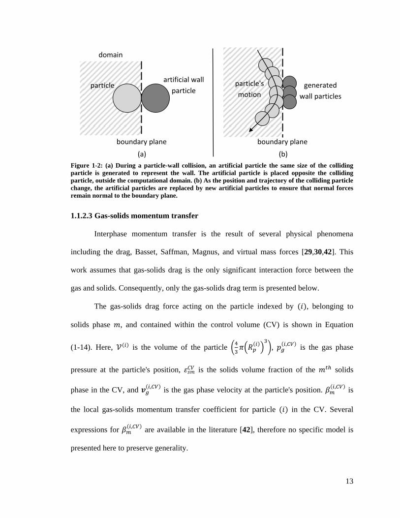
1.1.2.2 Particle-wall collision model

Particle-wall collisions are managed similarly to particle-particle collisions with

additional complexity arising from the need to represent the wall [41]. This work uses

artificial particles to act as the wall during a collision. When the surface of a particle

initiates contact with a boundary plane (wall), an artificial particle of the same size is

generated. The artificial particle is assigned the physical properties associated with the

wall and placed across the boundary, opposite the colliding particle, outside the

computational domain. This process is illustrated in Figure 1-2-(a). Once the forces

generated from the particle-wall collision are calculated, the artificial particle is removed.

After the position and trajectory of the colliding particle are updated, a new artificial

particle is created if the colliding particle remains in contact with the wall. This

procedure continues until the collision has evolved fully and the colliding particle is no

longer in contact with the wall, as illustrated in Figure 1-2-(b). This method of modeling

particle-wall collisions ensures that any normal forces generated during the collision are

always perpendicular to the boundary plane.

13

Figure 1-2: (a) During a particle-wall collision, an artificial particle the same size of the colliding

particle is generated to represent the wall. The artificial particle is placed opposite the colliding

particle, outside the computational domain. (b) As the position and trajectory of the colliding particle

change, the artificial particles are replaced by new artificial particles to ensure that normal forces

remain normal to the boundary plane.

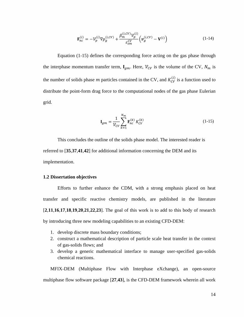
1.1.2.3 Gas-solids momentum transfer

Interphase momentum transfer is the result of several physical phenomena

including the drag, Basset, Saffman, Magnus, and virtual mass forces [29,30,42]. This

work assumes that gas-solids drag is the only significant interaction force between the

gas and solids. Consequently, only the gas-solids drag term is presented below.

The gas-solids drag force acting on the particle indexed by , belonging to

solids phase , and contained within the control volume (CV) is shown in Equation

(1-14). Here, is the volume of the particle

,

is the gas phase

pressure at the particle's position, is the solids volume fraction of the solids

phase in the CV, and

is the gas phase velocity at the particle's position.

is

the local gas-solids momentum transfer coefficient for particle in the CV. Several

expressions for

are available in the literature [42], therefore no specific model is

presented here to preserve generality.

artificial wall

particle particle

(a) (b)

boundary plane

particle's

motion generated

wall particles

boundary plane

domain

14

(1-14)

Equation (1-15) defines the corresponding force acting on the gas phase through

the interphase momentum transfer term, . Here, is the volume of the CV, is

the number of solids phase particles contained in the CV, and

is a function used to

distribute the point-form drag force to the computational nodes of the gas phase Eulerian

grid.

(1-15)

This concludes the outline of the solids phase model. The interested reader is

referred to [35,37,41,42] for additional information concerning the DEM and its

implementation.

1.2 Dissertation objectives

Efforts to further enhance the CDM, with a strong emphasis placed on heat

transfer and specific reactive chemistry models, are published in the literature

[2,11,16,17,18,19,20,21,22,23]. The goal of this work is to add to this body of research

by introducing three new modeling capabilities to an existing CFD-DEM:

1. develop discrete mass boundary conditions;

2. construct a mathematical description of particle scale heat transfer in the context

of gas-solids flows; and

3. develop a generic mathematical interface to manage user-specified gas-solids

chemical reactions.

MFIX-DEM (Multiphase Flow with Interphase eXchange), an open-source

multiphase flow software package [27,43], is the CFD-DEM framework wherein all work

15

is conducted. Accordingly, all programmatic efforts follow the FORTRAN90/95 coding

standard.

1.3 Document organization

Chapter 2 presents the algorithmic description of the discrete mass inflow and

outflow boundary conditions. Details concerning the implementation of the boundary

conditions into MFIX-DEM are discussed and two examples illustrating the behavior of

the discrete mass inflow boundary condition are given. Chapter 3 begins by defining the

three modes of heat transfer and the internal energy equation for a single, isothermal

particle. An examination of the assumption of isothermal particles is conducted. In the

subsequent sections, an analysis of contact conduction, particle-fluid-particle conduction,

particle-gas convection, and particle-environment radiation are presented. Each

investigation includes (1) a survey of models proposed for the specified mode of heat

transfer, and (2) a discussion detailing modifications made to the selected model. Finally,

the algorithmic implementation and verification of the selected heat transfer models are

given. In Chapter 4, a discussion of reactive chemistry is presented in conjunction with a

survey of previous efforts to incorporate reactive chemistry into the CFD-DEM. Then the

mathematical interface for managing user-defined chemical reactions and its

implementation into MFIX-DEM are outlined. Finally, a brief study verifying the

interface is discussed. Finally, in Chapter 5 a summary of this work’s efforts is presented

along with areas of interest for future investigations.

16

Chapter 2: Discrete mass boundary conditions

In mathematics, boundary conditions, like those of Neumann and Dirichlet, are

typically considered in the context of differential equations. However, in a discrete

element model (DEM), there is no natural analogue to specify the flux of solids into a

system. This investigation aims to develop a Neumann-like boundary condition algorithm

for introducing new solids into a simulation that employs the DEM. This work also

describes the construction of a mass outflow boundary region. The algorithms are termed

the discrete mass inflow boundary condition (DMIBC) and discrete mass outflow

boundary condition (DMOBC).

2.1 Introduction

Recall from Chapter 1 that the contact force scheme of Cundall and Strack [44] is

adopted for this work. In their model, mechanical elements are used to account for the

elastic, damping and rotational forces generated during a particle-particle collision. As

particles collide, the deformation of each particle’s shape is captured through an overlap

of their contact regions. The magnitude of the overlap is related to the scale of the forces

resulting from impact. As the collision evolves, the resultant forces are used to

recalculate the positions, trajectories, and rotational speeds of the particles.

Since the overlap between particles is used to determine the kinetic response to a

collision, a particle entering the system cannot be placed overlapping another particle.

This limitation is apparent if a DMIBC is defined along a domain region that is

associated with a high particle density, such as a packed bed. To avoid improper

placement of particles while retaining the ability to define a DMIBC along any region of

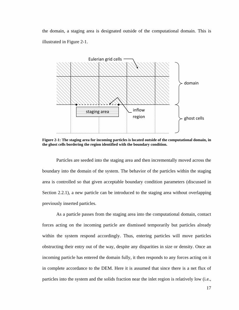
17

the domain, a staging area is designated outside of the computational domain. This is

illustrated in Figure 2-1.

Figure 2-1: The staging area for incoming particles is located outside of the computational domain, in

the ghost cells bordering the region identified with the boundary condition.

Particles are seeded into the staging area and then incrementally moved across the

boundary into the domain of the system. The behavior of the particles within the staging

area is controlled so that given acceptable boundary condition parameters (discussed in

Section 2.2.1), a new particle can be introduced to the staging area without overlapping

previously inserted particles.

As a particle passes from the staging area into the computational domain, contact

forces acting on the incoming particle are dismissed temporarily but particles already

within the system respond accordingly. Thus, entering particles will move particles

obstructing their entry out of the way, despite any disparities in size or density. Once an

incoming particle has entered the domain fully, it then responds to any forces acting on it

in complete accordance to the DEM. Here it is assumed that since there is a net flux of

particles into the system and the solids fraction near the inlet region is relatively low (i.e.,

staging area inflow

region

Eulerian grid cells

domain

ghost cells

18

not packed) for most situations [45,46], the overall effect of incoming particles neglecting

contact forces is negligible.

An outflow boundary condition for the DEM results in a modification of the

particle-wall collision algorithm. In its application, when a particle collides with a wall

region associated with an outlet, the collision force is ignored. This allows the particle to

move from the computational domain to a bordering ghost cell over a series of time steps.

Once the particle has exited the computational domain fully, all instances of the particle

are removed from memory.

2.2 DMIBC algorithm description

The DMIBC has two operating components. The first element is called during the

initialization of the software, wherein user provided data is checked for consistency, and

operational characteristics are determined. The second element is executed during the

simulation, and controls the placement and assignment of physical properties to incoming

particles. The two components of the algorithm are outlined below.

2.2.1 DMIBC initialization

To define the operational characteristics of a DMIBC, the physical properties and

feed rates of the incoming particles are specified. The physical properties of an incoming

particle are identified through its solids phase. As previously stated, the solids phase is

associated with the diameter, , and material density, , of a particle. Note, particles

belonging to the solids phase indexed by are identified by a subscript and are

referred to as ‘solids phase ’ particles. The feed rate for each solids phase is given by a

volumetric flow rate and bulk density, and , respectively. Here is the

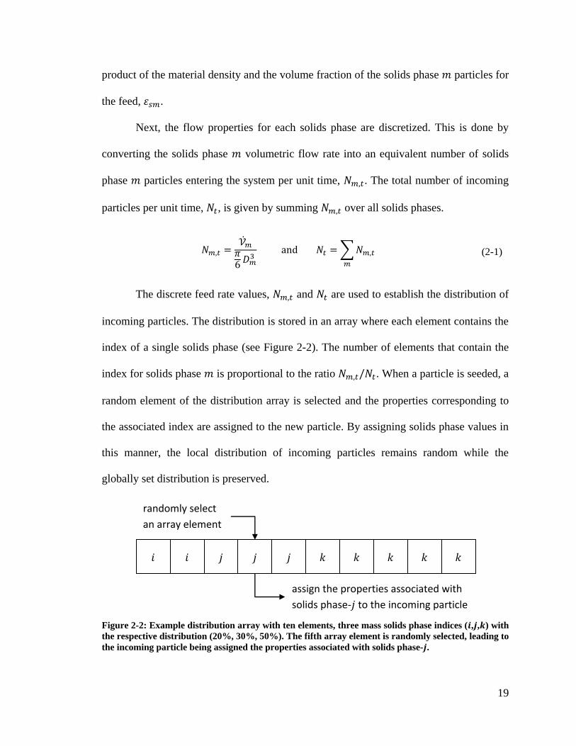
19

product of the material density and the volume fraction of the solids phase particles for

the feed, .

Next, the flow properties for each solids phase are discretized. This is done by

converting the solids phase volumetric flow rate into an equivalent number of solids

phase particles entering the system per unit time, . The total number of incoming

particles per unit time, , is given by summing over all solids phases.

(2-1)

The discrete feed rate values, and are used to establish the distribution of

incoming particles. The distribution is stored in an array where each element contains the

index of a single solids phase (see Figure 2-2). The number of elements that contain the

index for solids phase is proportional to the ratio . When a particle is seeded, a

random element of the distribution array is selected and the properties corresponding to

the associated index are assigned to the new particle. By assigning solids phase values in

this manner, the local distribution of incoming particles remains random while the

globally set distribution is preserved.

Figure 2-2: Example distribution array with ten elements, three mass solids phase indices ( , , ) with

the respective distribution (20%, 30%, 50%). The fifth array element is randomly selected, leading to

the incoming particle being assigned the properties associated with solids phase- .

randomly select

an array element

assign the properties associated with

solids phase- to the incoming particle

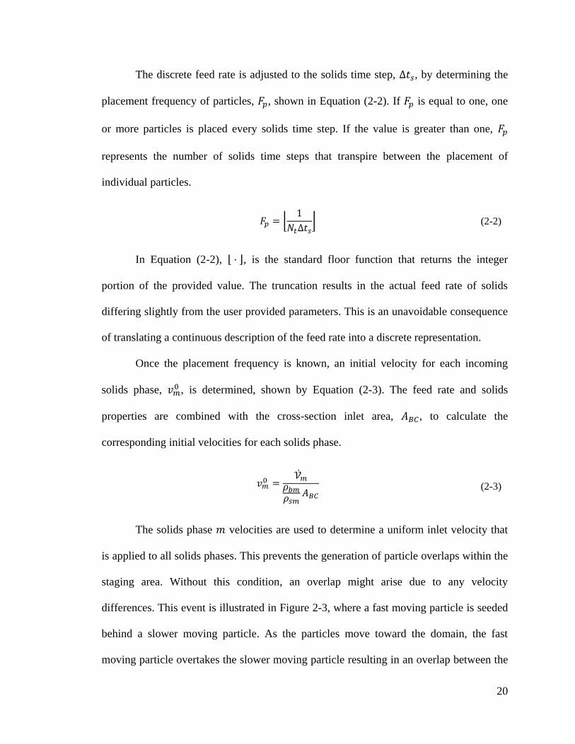
20

The discrete feed rate is adjusted to the solids time step, , by determining the

placement frequency of particles, , shown in Equation (2-2). If is equal to one, one

or more particles is placed every solids time step. If the value is greater than one,

represents the number of solids time steps that transpire between the placement of

individual particles.

(2-2)

In Equation (2-2), , is the standard floor function that returns the integer

portion of the provided value. The truncation results in the actual feed rate of solids

differing slightly from the user provided parameters. This is an unavoidable consequence

of translating a continuous description of the feed rate into a discrete representation.

Once the placement frequency is known, an initial velocity for each incoming

solids phase, , is determined, shown by Equation (2-3). The feed rate and solids

properties are combined with the cross-section inlet area, , to calculate the

corresponding initial velocities for each solids phase.

(2-3)

The solids phase velocities are used to determine a uniform inlet velocity that

is applied to all solids phases. This prevents the generation of particle overlaps within the

staging area. Without this condition, an overlap might arise due to any velocity

differences. This event is illustrated in Figure 2-3, where a fast moving particle is seeded

behind a slower moving particle. As the particles move toward the domain, the fast

moving particle overtakes the slower moving particle resulting in an overlap between the

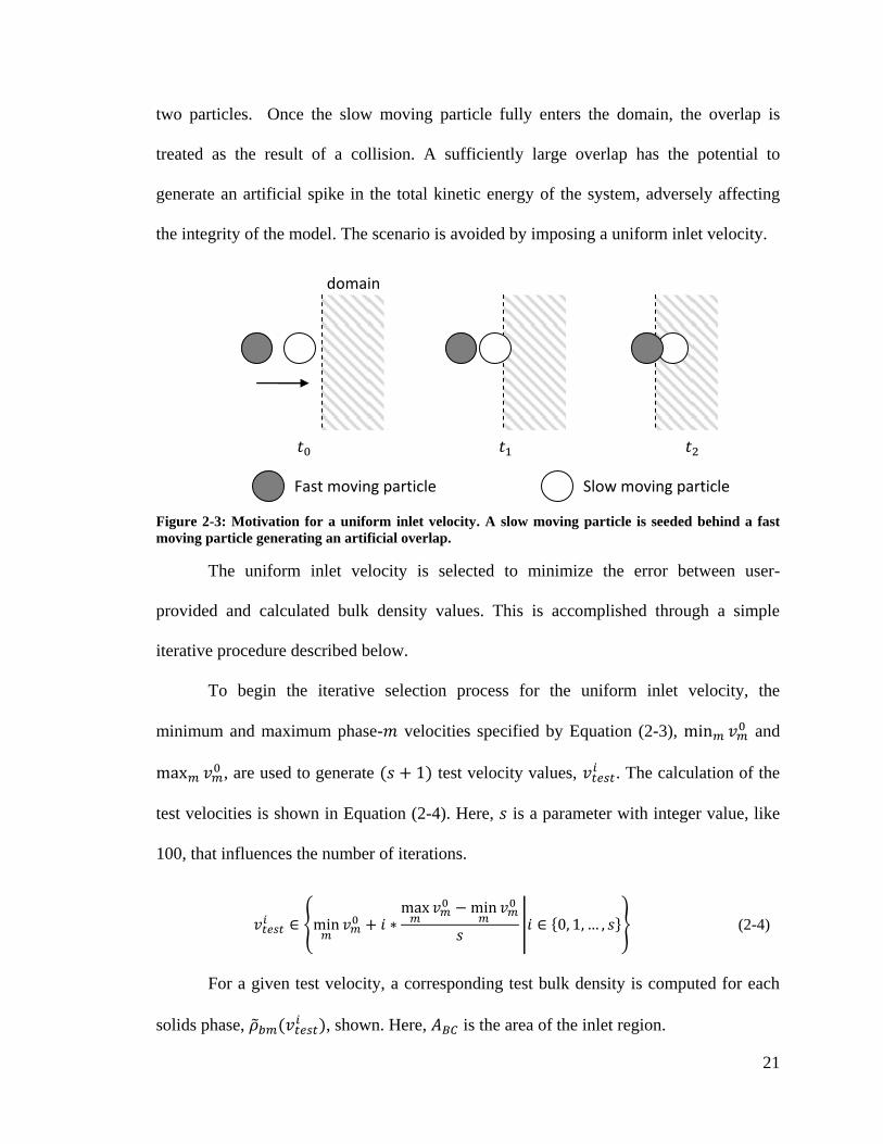
21

two particles. Once the slow moving particle fully enters the domain, the overlap is

treated as the result of a collision. A sufficiently large overlap has the potential to

generate an artificial spike in the total kinetic energy of the system, adversely affecting

the integrity of the model. The scenario is avoided by imposing a uniform inlet velocity.

Figure 2-3: Motivation for a uniform inlet velocity. A slow moving particle is seeded behind a fast

moving particle generating an artificial overlap.

The uniform inlet velocity is selected to minimize the error between user-

provided and calculated bulk density values. This is accomplished through a simple

iterative procedure described below.

To begin the iterative selection process for the uniform inlet velocity, the

minimum and maximum phase- velocities specified by Equation (2-3), and

, are used to generate test velocity values,

. The calculation of the

test velocities is shown in Equation (2-4). Here, is a parameter with integer value, like

100, that influences the number of iterations.

(2-4)

For a given test velocity, a corresponding test bulk density is computed for each

solids phase, , shown. Here, is the area of the inlet region.

domain

Fast moving particle Slow moving particle

22

(2-5)

At this point, the total error, , between the user-defined and newly

computed test bulk density values is calculated. The test velocity that produces the least

amount of total bulk density error is selected. This process is repeated with a new set of

test velocities established around the minimizing velocity of the previous iteration,

continuing until the difference between the results of two consecutive iterations is less

than a specified tolerance (e.g., ).

(2-6)

Finally, this optimized uniform inlet velocity is compared to two velocity values,

explained below. The first defines a lower bound on the inlet velocity, while the second

identifies the method used to seed incoming particles. These comparisons assure that the

user-defined inlet specifications are successfully managed, and determine which of the

two seeding algorithms, also presented below, is employed.

The lower bound on the inlet velocity is the minimum operational velocity, .

It coincides with an unmanageable situation where particles are seeded into the staging

area faster than they leave. Below a new particle may be seeded such that it

overlaps with an existing particle still within the staging area. Again, if the overlap is

sufficiently large, it may cause an artificial spike in the kinetic energy of the system.

To prevent particle overlap within the staging area, a sub-grid is constructed to

keep particles fully separated. The number of cells in the sub-grid, , depends on the

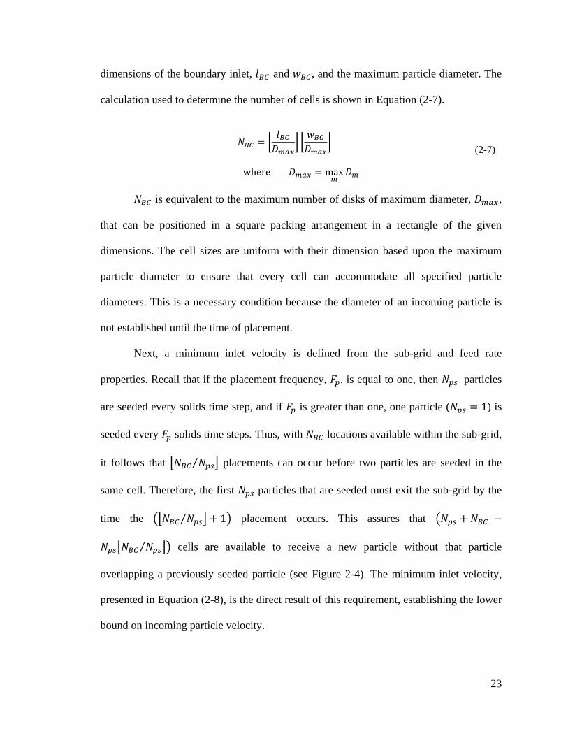
23

dimensions of the boundary inlet, and , and the maximum particle diameter. The

calculation used to determine the number of cells is shown in Equation (2-7).

(2-7)

is equivalent to the maximum number of disks of maximum diameter, ,

that can be positioned in a square packing arrangement in a rectangle of the given

dimensions. The cell sizes are uniform with their dimension based upon the maximum

particle diameter to ensure that every cell can accommodate all specified particle

diameters. This is a necessary condition because the diameter of an incoming particle is

not established until the time of placement.

Next, a minimum inlet velocity is defined from the sub-grid and feed rate

properties. Recall that if the placement frequency, , is equal to one, then particles

are seeded every solids time step, and if is greater than one, one particle ( ) is

seeded every solids time steps. Thus, with locations available within the sub-grid,

it follows that placements can occur before two particles are seeded in the

same cell. Therefore, the first particles that are seeded must exit the sub-grid by the

time the placement occurs. This assures that

cells are available to receive a new particle without that particle

overlapping a previously seeded particle (see Figure 2-4). The minimum inlet velocity,

presented in Equation (2-8), is the direct result of this requirement, establishing the lower

bound on incoming particle velocity.

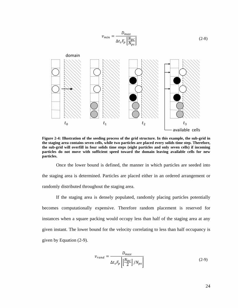
24

(2-8)

Figure 2-4: Illustration of the seeding process of the grid structure. In this example, the sub-grid in

the staging area contains seven cells, while two particles are placed every solids time step. Therefore,

the sub-grid will overfill in four solids time steps (eight particles and only seven cells) if incoming

particles do not move with sufficient speed toward the domain leaving available cells for new

particles.

Once the lower bound is defined, the manner in which particles are seeded into

the staging area is determined. Particles are placed either in an ordered arrangement or

randomly distributed throughout the staging area.

If the staging area is densely populated, randomly placing particles potentially

becomes computationally expensive. Therefore random placement is reserved for

instances when a square packing would occupy less than half of the staging area at any

given instant. The lower bound for the velocity correlating to less than half occupancy is

given by Equation (2-9).

(2-9)

domain

available cells

25

With the velocities and indentified, the placement method of particles

is determined. If the inlet velocity is between and , particles are placed in the

square packing arrangement defined by the grid structure imposed on the staging area. In

this instance a fill order for the grid cells is generated. (This pattern is repeated cyclically

to seed additional particles.)

For velocities greater than the particles are seeded via a guess-and-check

(random) method. First, a particle is tentatively assigned a random location within the

staging area. This position is independent of the sub-grid imposed on the staging area.

Then a check is conducted to test if the location causes particle overlap with inlet

particles that were previously seeded. If an overlap occurs, the particle is assigned a new

random location within the staging area. This process continues until the particle is

placed without any overlaps.

After a particle is seeded into the staging area, the ghost cell that contains the new

particle is determined (see Figure 2-1). The cells within the computational domain that

border those ghost cells in the inlet area are identified. Finally, a local search is

conducted that allows for particles already within the computational domain to identify

incoming particles as possible contact partners.

2.2.2 DMIBC operation

During a simulation, the placement frequency is used to calculate when the next

particle is seeded. During each solids time step, the current time value is compared to a

placement time, . If is less than or equal to the current solids time, a new particle is

seeded into the inlet region, and the next seeding time updated.

26

(2-10)

When a new particle is seeded, a flag is set identifying it as a new particle which

indicates the dismissal of any contact forces the particle is exposed to during entry. This

classification is maintained only until the particle has entered the computational domain

fully. As a result, entering (new) particles will push obstructing particles in the

computational domain away from the inlet.

Next, physical properties are assigned to the new particle through the appointment

of a solids phase index. As previously discussed, an element from the array representing

the incoming particle distribution is selected randomly. That array element contains the

index of a single solids phase. From this selection, the physical properties associated with

that index are assigned to the incoming particle.

After the solids phase is assigned, the center location of the new particle is

determined. For an inlet using an ordered placement scheme, the sub-grid cell that will

contain the new particle is identified. If the dimensions of the cell are larger than the

diameter of the particle, the particle is positioned randomly within the cell; the particles

that have delimited the cell dimensions are placed on cell-center. For an inlet using the

random placement, the sub-grid imposed on the staging area is discarded and a guess-

and-check process initiated. New locations within the staging area are assigned to the

particle until it is placed without overlapping another particle.

Finally, the ghost cell that contains the new particle is determined. A local search

is conducted allowing particles already within the computational domain to identify

incoming particles as possible contact partners.

27

The positions of incoming particles are monitored during each solids time step.

Once a particle has fully entered the computational domain, the flag identifying the

particle as new is removed. This reclassification allows the particle to react appropriately

to any force that acts upon it.

2.3 DMOBC algorithm description

The DMOBC operates in conjunction with the existing DEM framework. Namely,

during the simulation a check is performed on each particle to ascertain whether or not it

is in contact with any walls of the domain. If a particle is found to be in contact with a

wall that contains a discrete mass outlet, an additional check is initiated. If the contact

occurs at a region identified with a DMOBC, then the resulting particle-wall collision

forces are dismissed. This, in effect, makes the wall invisible to the particle, allowing it to

move out of the computational domain. This is synonymous with the process that allows

incoming particles to travel from the staging area into the computational domain.

The forces acting on an exiting particle are discarded once its center crosses the

domain boundary. This allows particles partially carried out of the computational domain

by grid-dependent forces (e.g., gas-solids drag) to continue exiting with a constant

velocity once these forces are no longer calculable.

A check is conducted at the end of each solids time step to identify particles that

have fully exited the computational domain. Once a particle is completely outside the

domain, a logical flag indicating the existence of the particle is removed, and the array

positions associated with that particle are cleared. The vacated array positions are

populated by information for incoming particles as-needed. By reusing the array

positions, the overall amount of system resources needed during a simulation are reduced.

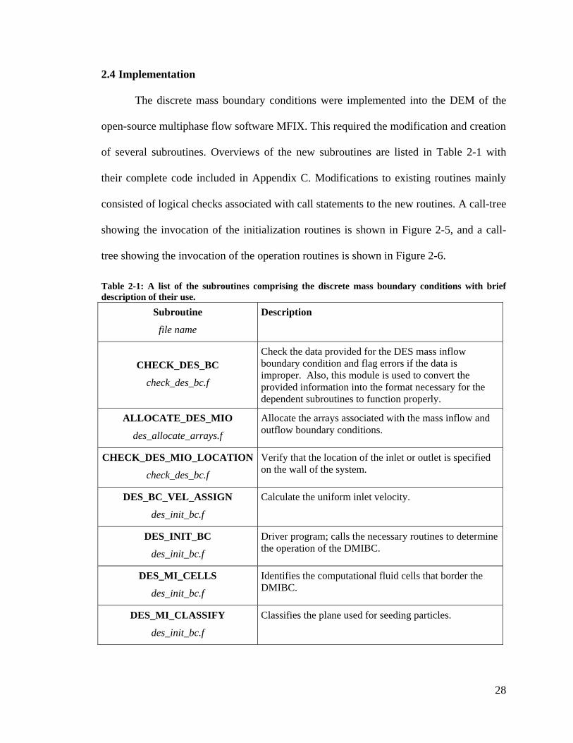
28

2.4 Implementation

The discrete mass boundary conditions were implemented into the DEM of the

open-source multiphase flow software MFIX. This required the modification and creation

of several subroutines. Overviews of the new subroutines are listed in Table 2-1 with

their complete code included in Appendix C. Modifications to existing routines mainly

consisted of logical checks associated with call statements to the new routines. A call-tree

showing the invocation of the initialization routines is shown in Figure 2-5, and a call-

tree showing the invocation of the operation routines is shown in Figure 2-6.

Table 2-1: A list of the subroutines comprising the discrete mass boundary conditions with brief

description of their use.

Subroutine

file name

Description

CHECK_DES_BC

check_des_bc.f

Check the data provided for the DES mass inflow

boundary condition and flag errors if the data is

improper. Also, this module is used to convert the

provided information into the format necessary for the

dependent subroutines to function properly.

ALLOCATE_DES_MIO

des_allocate_arrays.f

Allocate the arrays associated with the mass inflow and

outflow boundary conditions.

CHECK_DES_MIO_LOCATION

check_des_bc.f

Verify that the location of the inlet or outlet is specified

on the wall of the system.

DES_BC_VEL_ASSIGN

des_init_bc.f

Calculate the uniform inlet velocity.

DES_INIT_BC

des_init_bc.f

Driver program; calls the necessary routines to determine

the operation of the DMIBC.

DES_MI_CELLS

des_init_bc.f

Identifies the computational fluid cells that border the

DMIBC.

DES_MI_CLASSIFY

des_init_bc.f

Classifies the plane used for seeding particles.

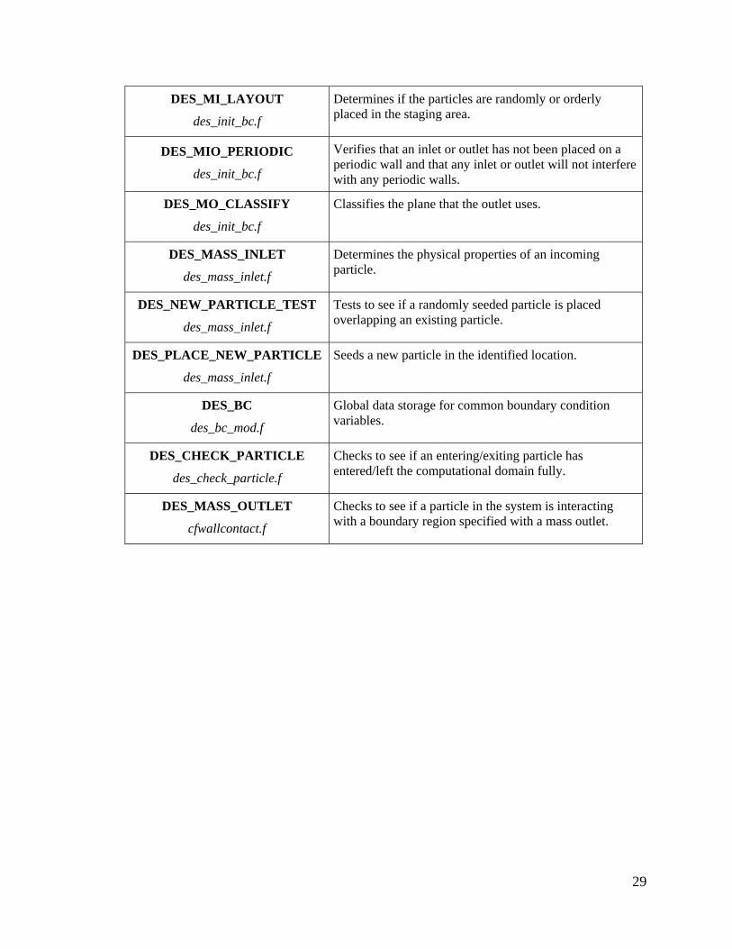
29

DES_MI_LAYOUT

des_init_bc.f

Determines if the particles are randomly or orderly

placed in the staging area.

DES_MIO_PERIODIC

des_init_bc.f

Verifies that an inlet or outlet has not been placed on a

periodic wall and that any inlet or outlet will not interfere

with any periodic walls.

DES_MO_CLASSIFY

des_init_bc.f

Classifies the plane that the outlet uses.

DES_MASS_INLET

des_mass_inlet.f

Determines the physical properties of an incoming

particle.

DES_NEW_PARTICLE_TEST

des_mass_inlet.f

Tests to see if a randomly seeded particle is placed

overlapping an existing particle.

DES_PLACE_NEW_PARTICLE

des_mass_inlet.f

Seeds a new particle in the identified location.

DES_BC

des_bc_mod.f

Global data storage for common boundary condition

variables.

DES_CHECK_PARTICLE

des_check_particle.f

Checks to see if an entering/exiting particle has

entered/left the computational domain fully.

DES_MASS_OUTLET

cfwallcontact.f

Checks to see if a particle in the system is interacting

with a boundary region specified with a mass outlet.

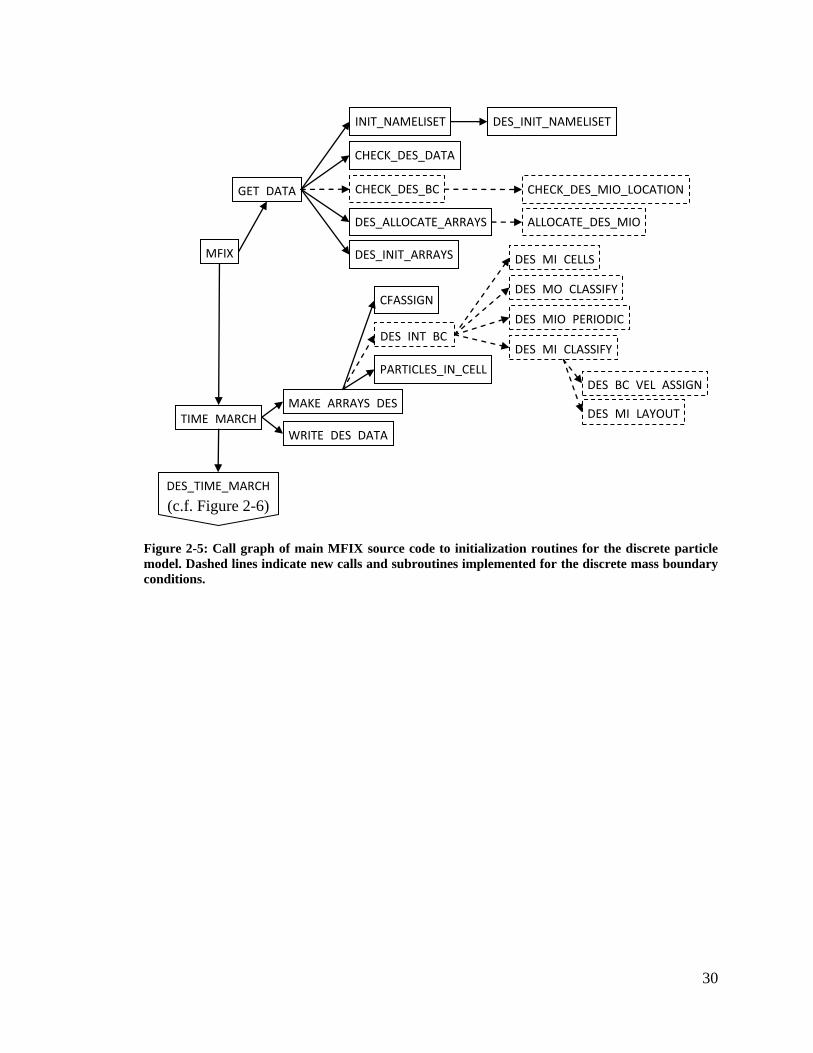
30

Figure 2-5: Call graph of main MFIX source code to initialization routines for the discrete particle

model. Dashed lines indicate new calls and subroutines implemented for the discrete mass boundary

conditions.

MFIX

GET_DATA

INIT_NAMELISET DES_INIT_NAMELISET

DES_ALLOCATE_ARRAYS

DES_INIT_ARRAYS

CHECK_DES_DATA

CHECK_DES_BC

ALLOCATE_DES_MIO

TIME_MARCH MAKE_ARRAYS_DES

WRITE_DES_DATA

DES_INT_BC

DES_MI_CELLS

DES_MO_CLASSIFY

DES_MI_LAYOUT

DES_MIO_PERIODIC

DES_MI_CLASSIFY

CHECK_DES_MIO_LOCATION

DES_BC_VEL_ASSIGN

DES_TIME_MARCH

(c.f. Figure 2-6)

PARTICLES_IN_CELL

CFASSIGN

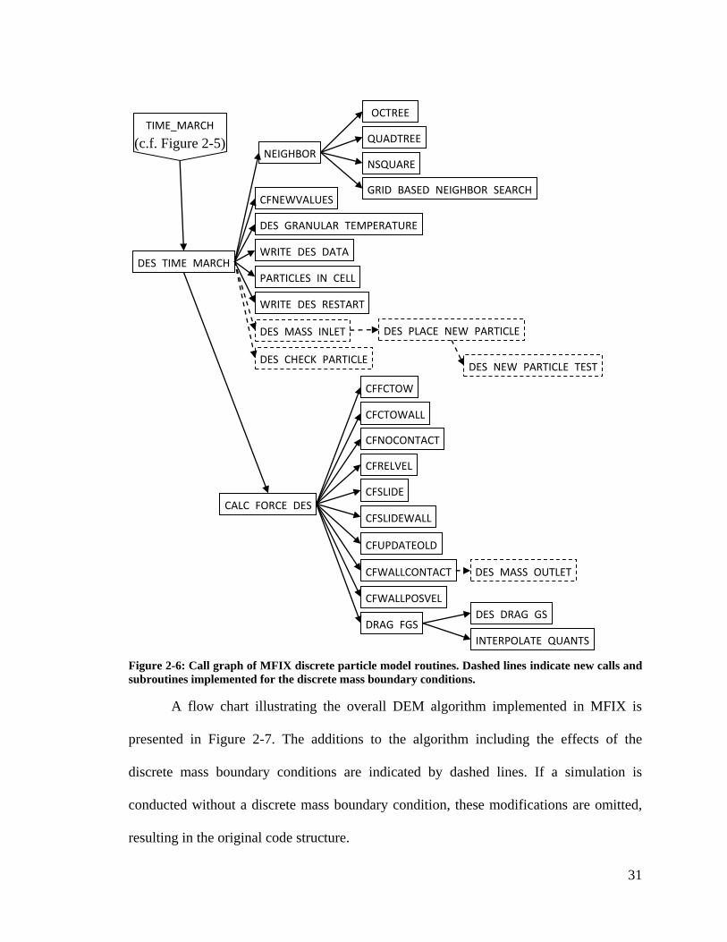
31

Figure 2-6: Call graph of MFIX discrete particle model routines. Dashed lines indicate new calls and

subroutines implemented for the discrete mass boundary conditions.

A flow chart illustrating the overall DEM algorithm implemented in MFIX is

presented in Figure 2-7. The additions to the algorithm including the effects of the

discrete mass boundary conditions are indicated by dashed lines. If a simulation is

conducted without a discrete mass boundary condition, these modifications are omitted,

resulting in the original code structure.

DES_TIME_MARCH

NEIGHBOR

CFNEWVALUES

DES_GRANULAR_TEMPERATURE

WRITE_DES_DATA

PARTICLES_IN_CELL

WRITE_DES_RESTART

CALC_FORCE_DES

NSQUARE

GRID_BASED_NEIGHBOR_SEARCH

QUADTREE

OCTREE

DES_MASS_INLET

DES_CHECK_PARTICLE DES_NEW_PARTICLE_TEST


CFCTOWALL

CFNOCONTACT

CFRELVEL

CFSLIDE

CFUPDATEOLD

CFWALLCONTACT

CFWALLPOSVEL

DRAG_FGS

CFFCTOW

CFSLIDEWALL

DES_MASS_OUTLET

INTERPOLATE_QUANTS

DES_DRAG_GS

TIME_MARCH

(c.f. Figure 2-5)

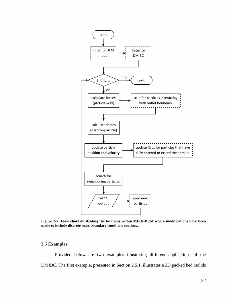
32

Figure 2-7: Flow chart illustrating the locations within MFIX-DEM where modifications have been

made to include discrete mass boundary condition routines.

2.5 Examples

Provided below are two examples illustrating different applications of the

DMIBC. The first example, presented in Section 2.5.1, illustrates a 2D packed bed (solids

Initialize DEM

model

Initialize

DMIBC

calculate forces

(particle-wall)

update particle

position and velocity

exit

start

no

yes

update flags for particles that have

fully entered or exited the domain

search for

neighboring particles

seed new

particles

calculate forces

(particle-particle)

scan for particles interacting

with outlet boundary

write

output

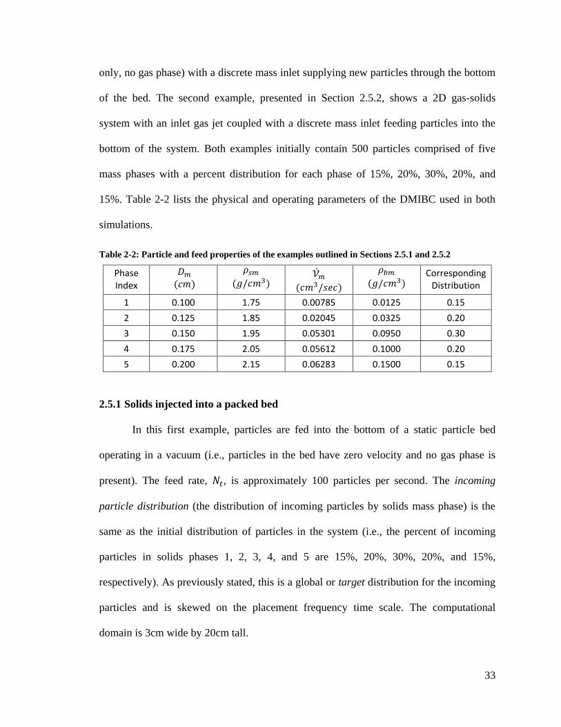
33

only, no gas phase) with a discrete mass inlet supplying new particles through the bottom

of the bed. The second example, presented in Section 2.5.2, shows a 2D gas-solids

system with an inlet gas jet coupled with a discrete mass inlet feeding particles into the

bottom of the system. Both examples initially contain 500 particles comprised of five

mass phases with a percent distribution for each phase of 15%, 20%, 30%, 20%, and

15%. Table 2-2 lists the physical and operating parameters of the DMIBC used in both

simulations.

Table 2-2: Particle and feed properties of the examples outlined in Sections 2.5.1 and 2.5.2

Phase Index

Corresponding Distribution

1 0.100 1.75 0.00785 0.0125 0.15

2 0.125 1.85 0.02045 0.0325 0.20

3 0.150 1.95 0.05301 0.0950 0.30

4 0.175 2.05 0.05612 0.1000 0.20

5 0.200 2.15 0.06283 0.1500 0.15

2.5.1 Solids injected into a packed bed

In this first example, particles are fed into the bottom of a static particle bed

operating in a vacuum (i.e., particles in the bed have zero velocity and no gas phase is

present). The feed rate, , is approximately 100 particles per second. The incoming

particle distribution (the distribution of incoming particles by solids mass phase) is the

same as the initial distribution of particles in the system (i.e., the percent of incoming

particles in solids phases 1, 2, 3, 4, and 5 are 15%, 20%, 30%, 20%, and 15%,

respectively). As previously stated, this is a global or target distribution for the incoming

particles and is skewed on the placement frequency time scale. The computational

domain is 3cm wide by 20cm tall.

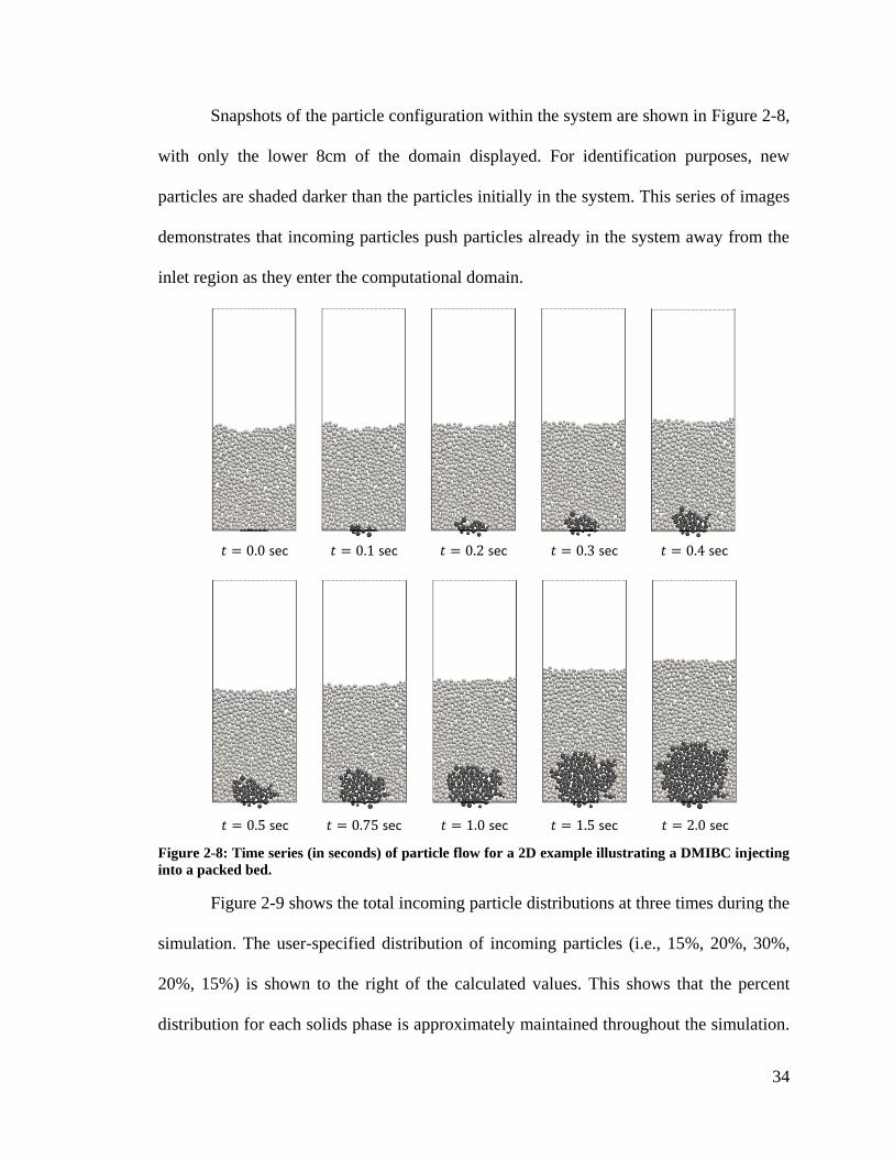
34

Snapshots of the particle configuration within the system are shown in Figure 2-8,

with only the lower 8cm of the domain displayed. For identification purposes, new

particles are shaded darker than the particles initially in the system. This series of images

demonstrates that incoming particles push particles already in the system away from the

inlet region as they enter the computational domain.

Figure 2-8: Time series (in seconds) of particle flow for a 2D example illustrating a DMIBC injecting

into a packed bed.

Figure 2-9 shows the total incoming particle distributions at three times during the

simulation. The user-specified distribution of incoming particles (i.e., 15%, 20%, 30%,

20%, 15%) is shown to the right of the calculated values. This shows that the percent

distribution for each solids phase is approximately maintained throughout the simulation.

sec sec sec sec sec

sec sec sec sec sec

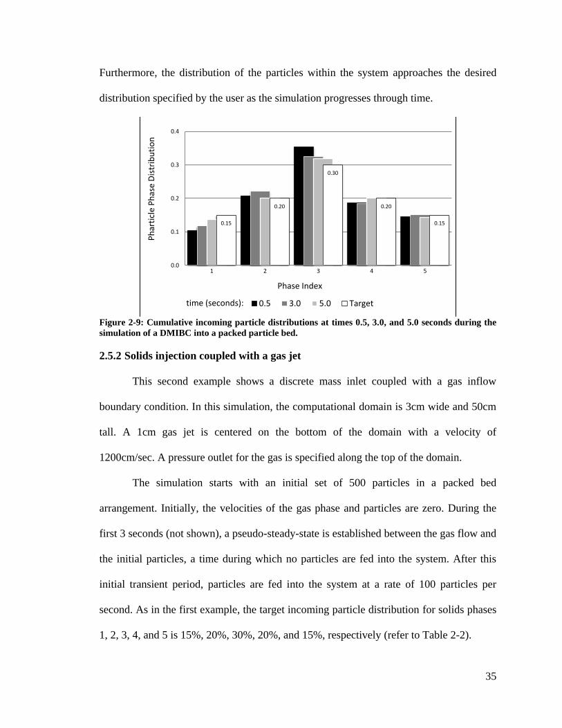
35

Furthermore, the distribution of the particles within the system approaches the desired

distribution specified by the user as the simulation progresses through time.

Figure 2-9: Cumulative incoming particle distributions at times 0.5, 3.0, and 5.0 seconds during the

simulation of a DMIBC into a packed particle bed.

2.5.2 Solids injection coupled with a gas jet

This second example shows a discrete mass inlet coupled with a gas inflow

boundary condition. In this simulation, the computational domain is 3cm wide and 50cm

tall. A 1cm gas jet is centered on the bottom of the domain with a velocity of

1200cm/sec. A pressure outlet for the gas is specified along the top of the domain.

The simulation starts with an initial set of 500 particles in a packed bed

arrangement. Initially, the velocities of the gas phase and particles are zero. During the

first 3 seconds (not shown), a pseudo-steady-state is established between the gas flow and

the initial particles, a time during which no particles are fed into the system. After this

initial transient period, particles are fed into the system at a rate of 100 particles per

second. As in the first example, the target incoming particle distribution for solids phases

1, 2, 3, 4, and 5 is 15%, 20%, 30%, 20%, and 15%, respectively (refer to Table 2-2).

0.15

0.20

0.30

0.20

0.15

0.0

0.1

0.2

0.3

0.4

1 2 3 4 5

Ph

arti

cle

Ph

ase

Dis

trib

uti

on

Phase Index

0.5 3.0 5.0 Target time (seconds):

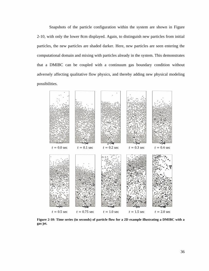
36

Snapshots of the particle configuration within the system are shown in Figure

2-10, with only the lower 8cm displayed. Again, to distinguish new particles from initial

particles, the new particles are shaded darker. Here, new particles are seen entering the

computational domain and mixing with particles already in the system. This demonstrates

that a DMIBC can be coupled with a continuum gas boundary condition without

adversely affecting qualitative flow physics, and thereby adding new physical modeling

possibilities.

Figure 2-10: Time series (in seconds) of particle flow for a 2D example illustrating a DMIBC with a

gas jet.

sec sec sec sec sec

sec sec sec sec sec

37

The distribution of incoming particles (not shown) closely matches the results

from the first example. This is expected since both inlets are defined by the same flow

properties.

2.6 Conclusions

The current MFIX-DEM code was modified to include DMIBC and DMOBC.

This allows models of more dynamic gas-solids systems by assigning user defined

boundary conditions to the computational domain. The new algorithmic features have

potential for use in simulations where particles enter as feedstock, like coal in a

gasification model, or systems where particles are recycled, like in a circulating fluidized

bed model.

38

Chapter 3: Particle heat transfer

Particle-particle and particle-gas heat transfer in gas-solids systems occur in the

forms of conduction, convection, and radiation. The goal of this investigation is to define

a mathematical model for each type of heat transfer and successfully implement the

selected models into MFIX-DEM, an existing CFD-DEM.

This chapter begins by briefly defining the three modes of heat transfer and

introducing the internal energy equation for a single, isothermal particle in Section 3.1.

An examination into the assumption of isothermal particles is included. In the subsequent

sections, an analysis of contact conduction (Section 3.2), particle-fluid-particle

conduction (Section 3.3), particle-gas convection (Section 3.4), and particle-environment

radiation (Section 3.5) are presented. Each investigation includes (1) a survey of models

proposed in the literature, and (2) a discussion detailing modifications made to the

selected model. Finally, the algorithmic implementation and verification of the selected

heat transfer models are given in Sections 3.6 and 3.7.

3.1 Foundations for particle heat transfer

In this section the physical mechanisms of conduction, convection, and radiation,

including a characterization of their contribution to particle heat transfer in gas-solids

systems are presented briefly. Additional details concerning the fundamentals of heat

transfer are found in reference [47]. The assumption of isothermal particles employed in

this work is then examined. Finally, the internal energy equation of a single, isothermal

particle is introduced.

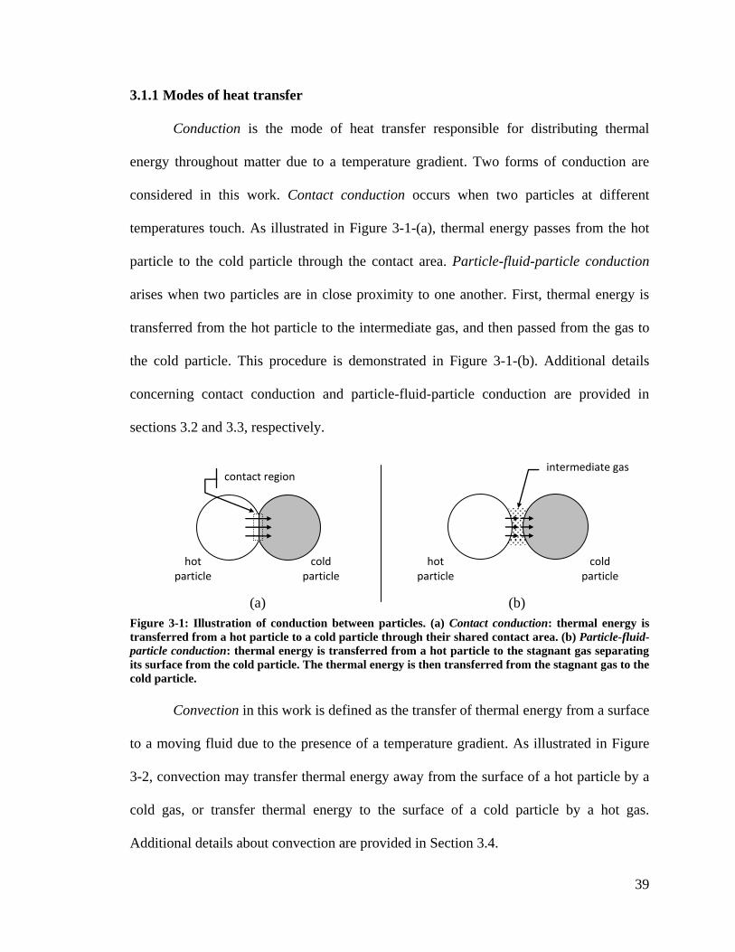
39

3.1.1 Modes of heat transfer

Conduction is the mode of heat transfer responsible for distributing thermal

energy throughout matter due to a temperature gradient. Two forms of conduction are

considered in this work. Contact conduction occurs when two particles at different

temperatures touch. As illustrated in Figure 3-1-(a), thermal energy passes from the hot

particle to the cold particle through the contact area. Particle-fluid-particle conduction

arises when two particles are in close proximity to one another. First, thermal energy is

transferred from the hot particle to the intermediate gas, and then passed from the gas to

the cold particle. This procedure is demonstrated in Figure 3-1-(b). Additional details

concerning contact conduction and particle-fluid-particle conduction are provided in

sections 3.2 and 3.3, respectively.

Figure 3-1: Illustration of conduction between particles. (a) Contact conduction: thermal energy is

transferred from a hot particle to a cold particle through their shared contact area. (b) Particle-fluid-

particle conduction: thermal energy is transferred from a hot particle to the stagnant gas separating

its surface from the cold particle. The thermal energy is then transferred from the stagnant gas to the

cold particle.

Convection in this work is defined as the transfer of thermal energy from a surface

to a moving fluid due to the presence of a temperature gradient. As illustrated in Figure

3-2, convection may transfer thermal energy away from the surface of a hot particle by a

cold gas, or transfer thermal energy to the surface of a cold particle by a hot gas.

Additional details about convection are provided in Section 3.4.

contact region

cold particle

(a)

hot particle

(b)

intermediate gas

cold particle

hot particle

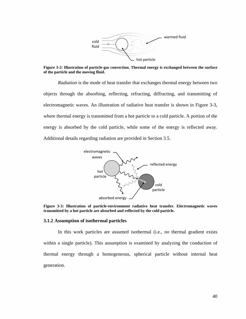
40

Figure 3-2: Illustration of particle-gas convection. Thermal energy is exchanged between the surface

of the particle and the moving fluid.

Radiation is the mode of heat transfer that exchanges thermal energy between two

objects through the absorbing, reflecting, refracting, diffracting, and transmitting of

electromagnetic waves. An illustration of radiative heat transfer is shown in Figure 3-3,

where thermal energy is transmitted from a hot particle to a cold particle. A portion of the

energy is absorbed by the cold particle, while some of the energy is reflected away.

Additional details regarding radiation are provided in Section 3.5.

Figure 3-3: Illustration of particle-environment radiative heat transfer. Electromagnetic waves

transmitted by a hot particle are absorbed and reflected by the cold particle.

3.1.2 Assumption of isothermal particles

In this work particles are assumed isothermal (i.e., no thermal gradient exists

within a single particle). This assumption is examined by analyzing the conduction of

thermal energy through a homogeneous, spherical particle without internal heat

generation.

cold particle

reflected energy

electromagnetic

waves

hot particle

absorbed energy

cold fluid

hot particle

warmed fluid

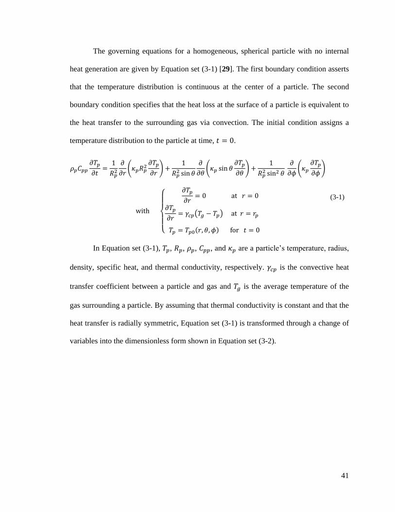
41

The governing equations for a homogeneous, spherical particle with no internal

heat generation are given by Equation set (3-1) [29]. The first boundary condition asserts

that the temperature distribution is continuous at the center of a particle. The second

boundary condition specifies that the heat loss at the surface of a particle is equivalent to

the heat transfer to the surrounding gas via convection. The initial condition assigns a

temperature distribution to the particle at time, .

(3-1)

In Equation set (3-1), , , , , and are a particle’s temperature, radius,

density, specific heat, and thermal conductivity, respectively. is the convective heat

transfer coefficient between a particle and gas and is the average temperature of the

gas surrounding a particle. By assuming that thermal conductivity is constant and that the

heat transfer is radially symmetric, Equation set (3-1) is transformed through a change of

variables into the dimensionless form shown in Equation set (3-2).

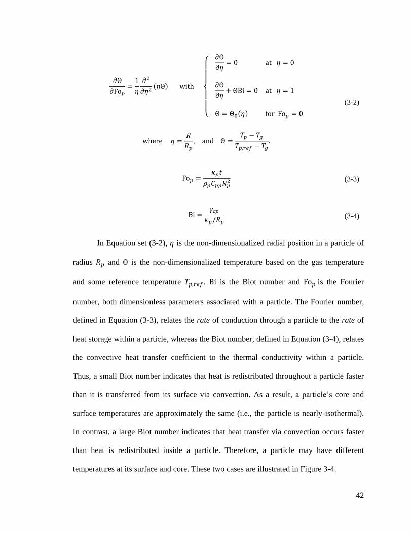
42

(3-2)

(3-3)

(3-4)

In Equation set (3-2), is the non-dimensionalized radial position in a particle of

radius and is the non-dimensionalized temperature based on the gas temperature

and some reference temperature . is the Biot number and is the Fourier

number, both dimensionless parameters associated with a particle. The Fourier number,

defined in Equation (3-3), relates the rate of conduction through a particle to the rate of

heat storage within a particle, whereas the Biot number, defined in Equation (3-4), relates

the convective heat transfer coefficient to the thermal conductivity within a particle.

Thus, a small Biot number indicates that heat is redistributed throughout a particle faster

than it is transferred from its surface via convection. As a result, a particle’s core and

surface temperatures are approximately the same (i.e., the particle is nearly-isothermal).

In contrast, a large Biot number indicates that heat transfer via convection occurs faster

than heat is redistributed inside a particle. Therefore, a particle may have different

temperatures at its surface and core. These two cases are illustrated in Figure 3-4.

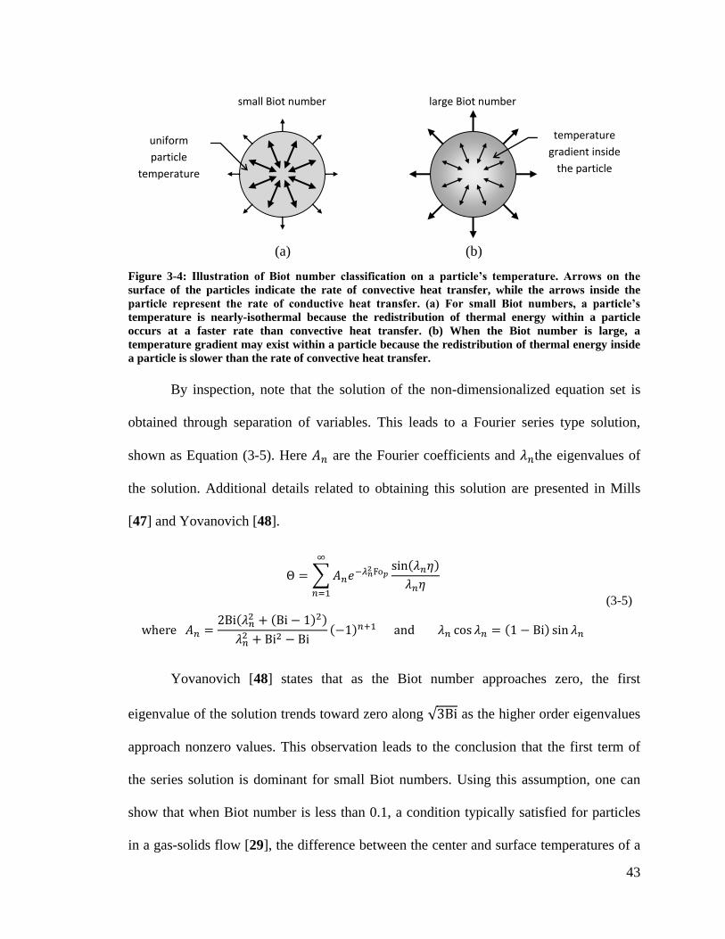
43

Figure 3-4: Illustration of Biot number classification on a particle’s temperature. Arrows on the

surface of the particles indicate the rate of convective heat transfer, while the arrows inside the

particle represent the rate of conductive heat transfer. (a) For small Biot numbers, a particle’s

temperature is nearly-isothermal because the redistribution of thermal energy within a particle

occurs at a faster rate than convective heat transfer. (b) When the Biot number is large, a

temperature gradient may exist within a particle because the redistribution of thermal energy inside

a particle is slower than the rate of convective heat transfer.

By inspection, note that the solution of the non-dimensionalized equation set is

obtained through separation of variables. This leads to a Fourier series type solution,

shown as Equation (3-5). Here are the Fourier coefficients and the eigenvalues of

the solution. Additional details related to obtaining this solution are presented in Mills

[47] and Yovanovich [48].

(3-5)

Yovanovich [48] states that as the Biot number approaches zero, the first

eigenvalue of the solution trends toward zero along as the higher order eigenvalues

approach nonzero values. This observation leads to the conclusion that the first term of

the series solution is dominant for small Biot numbers. Using this assumption, one can

show that when Biot number is less than 0.1, a condition typically satisfied for particles

in a gas-solids flow [29], the difference between the center and surface temperatures of a

(a) (b)

large Biot number small Biot number

temperature

gradient inside

the particle

uniform

particle

temperature

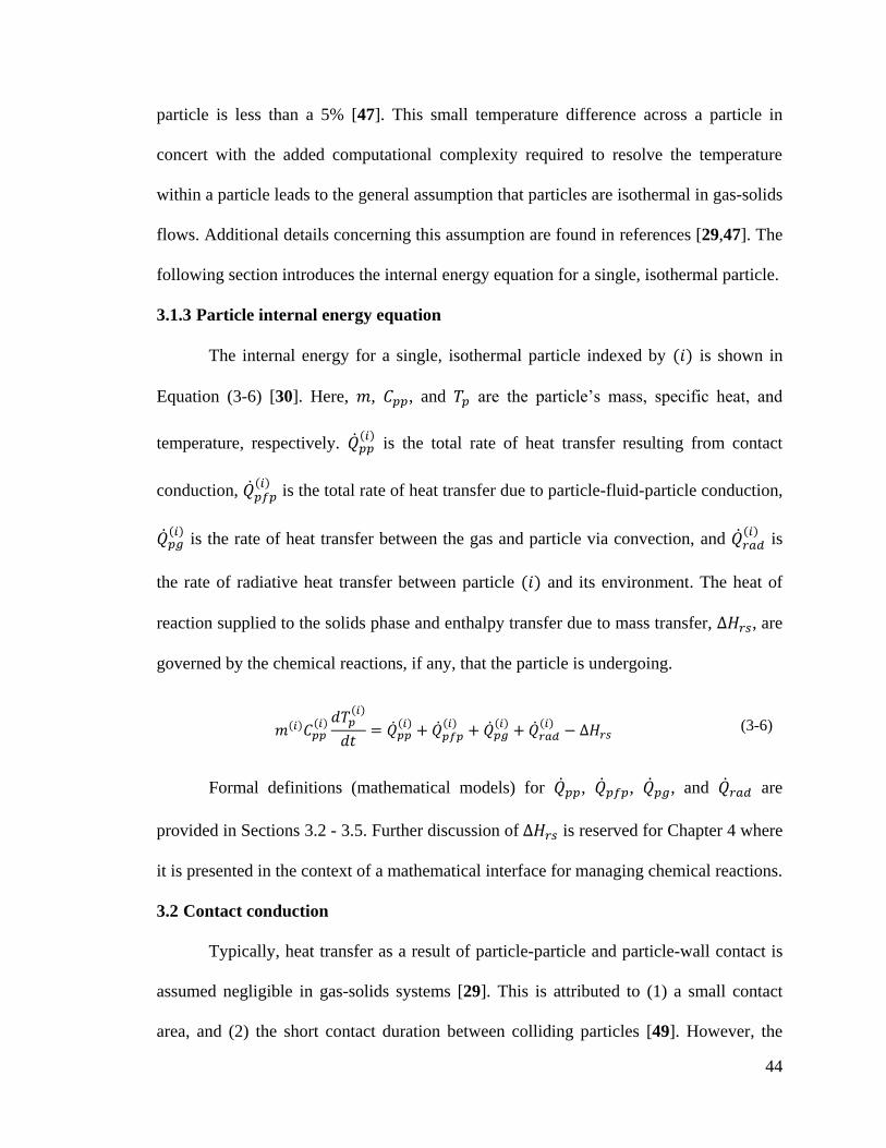
44

particle is less than a 5% [47]. This small temperature difference across a particle in

concert with the added computational complexity required to resolve the temperature

within a particle leads to the general assumption that particles are isothermal in gas-solids

flows. Additional details concerning this assumption are found in references [29,47]. The

following section introduces the internal energy equation for a single, isothermal particle.

3.1.3 Particle internal energy equation

The internal energy for a single, isothermal particle indexed by is shown in

Equation (3-6) [30]. Here, , , and are the particle’s mass, specific heat, and

temperature, respectively.

is the total rate of heat transfer resulting from contact

conduction,

is the total rate of heat transfer due to particle-fluid-particle conduction,

is the rate of heat transfer between the gas and particle via convection, and

is

the rate of radiative heat transfer between particle and its environment. The heat of

reaction supplied to the solids phase and enthalpy transfer due to mass transfer, , are

governed by the chemical reactions, if any, that the particle is undergoing.

(3-6)

Formal definitions (mathematical models) for ,

, , and

are

provided in Sections 3.2 - 3.5. Further discussion of is reserved for Chapter 4 where

it is presented in the context of a mathematical interface for managing chemical reactions.

3.2 Contact conduction

Typically, heat transfer as a result of particle-particle and particle-wall contact is

assumed negligible in gas-solids systems [29]. This is attributed to (1) a small contact

area, and (2) the short contact duration between colliding particles [49]. However, the

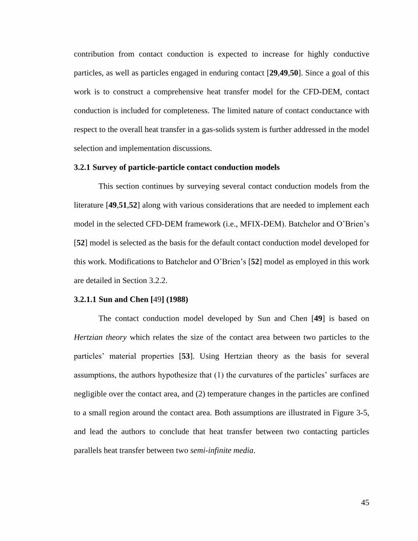
45

contribution from contact conduction is expected to increase for highly conductive

particles, as well as particles engaged in enduring contact [29,49,50]. Since a goal of this

work is to construct a comprehensive heat transfer model for the CFD-DEM, contact

conduction is included for completeness. The limited nature of contact conductance with

respect to the overall heat transfer in a gas-solids system is further addressed in the model

selection and implementation discussions.

3.2.1 Survey of particle-particle contact conduction models

This section continues by surveying several contact conduction models from the

literature [49,51,52] along with various considerations that are needed to implement each

model in the selected CFD-DEM framework (i.e., MFIX-DEM). Batchelor and O’Brien’s

[52] model is selected as the basis for the default contact conduction model developed for

this work. Modifications to Batchelor and O’Brien’s [52] model as employed in this work

are detailed in Section 3.2.2.

3.2.1.1 Sun and Chen [49] (1988)

The contact conduction model developed by Sun and Chen [49] is based on

Hertzian theory which relates the size of the contact area between two particles to the

particles’ material properties [53]. Using Hertzian theory as the basis for several

assumptions, the authors hypothesize that (1) the curvatures of the particles’ surfaces are

negligible over the contact area, and (2) temperature changes in the particles are confined

to a small region around the contact area. Both assumptions are illustrated in Figure 3-5,

and lead the authors to conclude that heat transfer between two contacting particles

parallels heat transfer between two semi-infinite media.

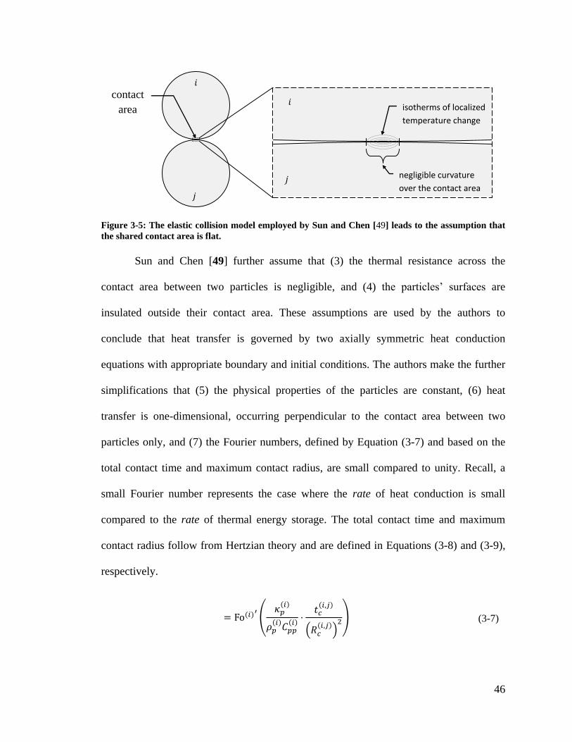
46

Figure 3-5: The elastic collision model employed by Sun and Chen [49] leads to the assumption that

the shared contact area is flat.

Sun and Chen [49] further assume that (3) the thermal resistance across the

contact area between two particles is negligible, and (4) the particles’ surfaces are

insulated outside their contact area. These assumptions are used by the authors to

conclude that heat transfer is governed by two axially symmetric heat conduction

equations with appropriate boundary and initial conditions. The authors make the further

simplifications that (5) the physical properties of the particles are constant, (6) heat

transfer is one-dimensional, occurring perpendicular to the contact area between two

particles only, and (7) the Fourier numbers, defined by Equation (3-7) and based on the

total contact time and maximum contact radius, are small compared to unity. Recall, a

small Fourier number represents the case where the rate of heat conduction is small

compared to the rate of thermal energy storage. The total contact time and maximum

contact radius follow from Hertzian theory and are defined in Equations (3-8) and (3-9),

respectively.

(3-7)

contact

area

isotherms of localized

temperature change

negligible curvature

over the contact area

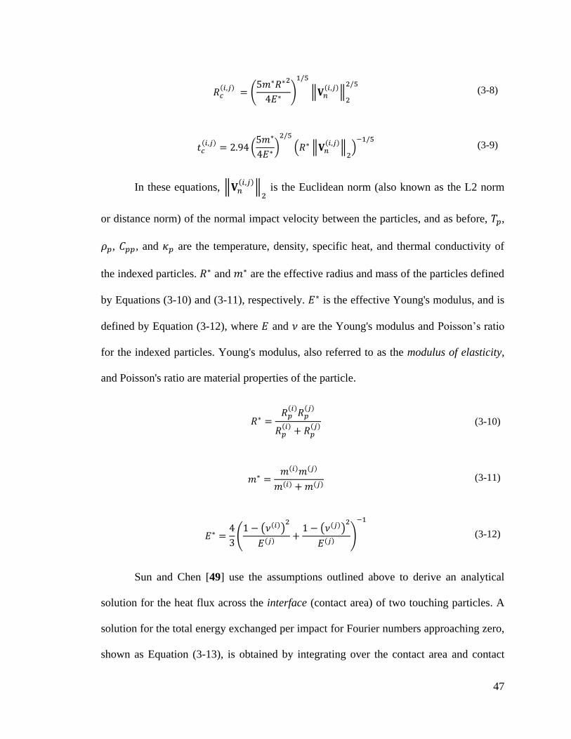
47

(3-8)

(3-9)

In these equations,

is the Euclidean norm (also known as the L2 norm

or distance norm) of the normal impact velocity between the particles, and as before, ,

, , and are the temperature, density, specific heat, and thermal conductivity of

the indexed particles. and are the effective radius and mass of the particles defined

by Equations (3-10) and (3-11), respectively. is the effective Young's modulus, and is

defined by Equation (3-12), where and are the Young's modulus and Poisson’s ratio

for the indexed particles. Young's modulus, also referred to as the modulus of elasticity,

and Poisson's ratio are material properties of the particle.

(3-10)

(3-11)

(3-12)

Sun and Chen [49] use the assumptions outlined above to derive an analytical

solution for the heat flux across the interface (contact area) of two touching particles. A

solution for the total energy exchanged per impact for Fourier numbers approaching zero,

shown as Equation (3-13), is obtained by integrating over the contact area and contact

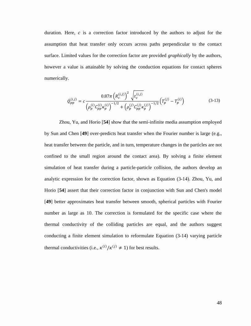
48

duration. Here, is a correction factor introduced by the authors to adjust for the

assumption that heat transfer only occurs across paths perpendicular to the contact

surface. Limited values for the correction factor are provided graphically by the authors,

however a value is attainable by solving the conduction equations for contact spheres

numerically.

(3-13)

Zhou, Yu, and Horio [54] show that the semi-infinite media assumption employed

by Sun and Chen [49] over-predicts heat transfer when the Fourier number is large (e.g.,

heat transfer between the particle, and in turn, temperature changes in the particles are not

confined to the small region around the contact area). By solving a finite element

simulation of heat transfer during a particle-particle collision, the authors develop an

analytic expression for the correction factor, shown as Equation (3-14). Zhou, Yu, and

Horio [54] assert that their correction factor in conjunction with Sun and Chen's model

[49] better approximates heat transfer between smooth, spherical particles with Fourier

number as large as 10. The correction is formulated for the specific case where the

thermal conductivity of the colliding particles are equal, and the authors suggest

conducting a finite element simulation to reformulate Equation (3-14) varying particle

thermal conductivities (i.e., ) for best results.

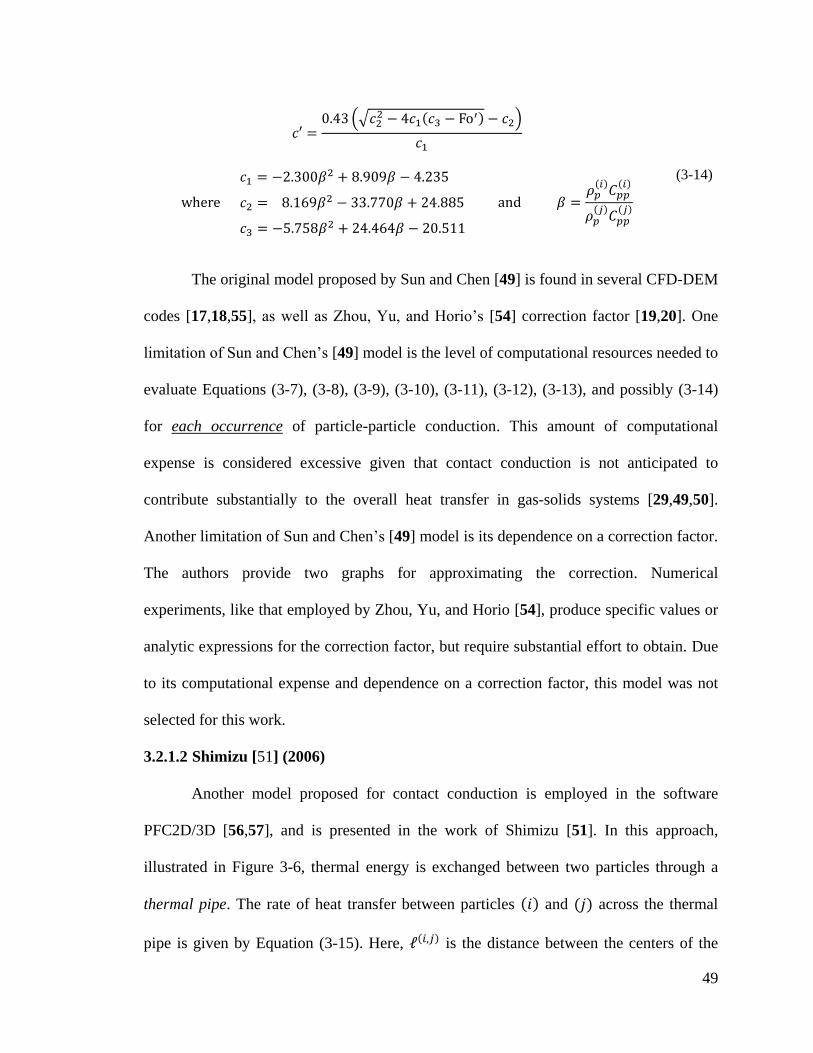
49

(3-14)

The original model proposed by Sun and Chen [49] is found in several CFD-DEM

codes [17,18,55], as well as Zhou, Yu, and Horio’s [54] correction factor [19,20]. One

limitation of Sun and Chen’s [49] model is the level of computational resources needed to

evaluate Equations (3-7), (3-8), (3-9), (3-10), (3-11), (3-12), (3-13), and possibly (3-14)

for each occurrence of particle-particle conduction. This amount of computational

expense is considered excessive given that contact conduction is not anticipated to

contribute substantially to the overall heat transfer in gas-solids systems [29,49,50].

Another limitation of Sun and Chen’s [49] model is its dependence on a correction factor.

The authors provide two graphs for approximating the correction. Numerical

experiments, like that employed by Zhou, Yu, and Horio [54], produce specific values or

analytic expressions for the correction factor, but require substantial effort to obtain. Due

to its computational expense and dependence on a correction factor, this model was not

selected for this work.

3.2.1.2 Shimizu [51] (2006)

Another model proposed for contact conduction is employed in the software

PFC2D/3D [56,57], and is presented in the work of Shimizu [51]. In this approach,

illustrated in Figure 3-6, thermal energy is exchanged between two particles through a

thermal pipe. The rate of heat transfer between particles and across the thermal

pipe is given by Equation (3-15). Here, is the distance between the centers of the

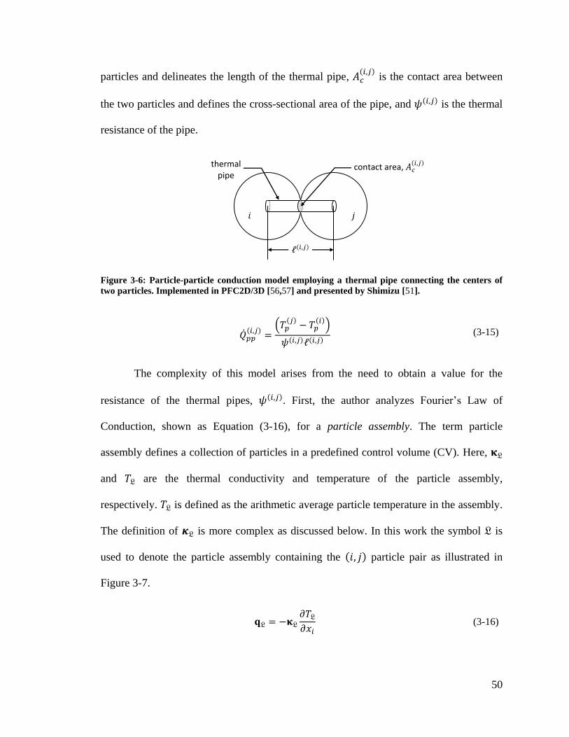
50

particles and delineates the length of the thermal pipe,

is the contact area between

the two particles and defines the cross-sectional area of the pipe, and is the thermal

resistance of the pipe.

Figure 3-6: Particle-particle conduction model employing a thermal pipe connecting the centers of

two particles. Implemented in PFC2D/3D [56,57] and presented by Shimizu [51].

(3-15)

The complexity of this model arises from the need to obtain a value for the

resistance of the thermal pipes, . First, the author analyzes Fourier’s Law of

Conduction, shown as Equation (3-16), for a particle assembly. The term particle

assembly defines a collection of particles in a predefined control volume (CV). Here,

and are the thermal conductivity and temperature of the particle assembly,

respectively. is defined as the arithmetic average particle temperature in the assembly.

The definition of is more complex as discussed below. In this work the symbol is

used to denote the particle assembly containing the particle pair as illustrated in

Figure 3-7.

(3-16)

contact area,

thermal pipe

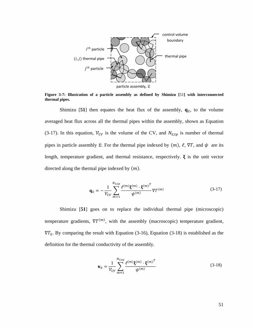
51

Figure 3-7: Illustration of a particle assembly as defined by Shimizu [51] with interconnected

thermal pipes.

Shimizu [51] then equates the heat flux of the assembly, , to the volume

averaged heat flux across all the thermal pipes within the assembly, shown as Equation

(3-17). In this equation, is the volume of the CV, and is number of thermal

pipes in particle assembly . For the thermal pipe indexed by , , , and are its

length, temperature gradient, and thermal resistance, respectively. is the unit vector

directed along the thermal pipe indexed by .

(3-17)

Shimizu [51] goes on to replace the individual thermal pipe (microscopic)

temperature gradients, , with the assembly (macroscopic) temperature gradient,

. By comparing the result with Equation (3-16), Equation (3-18) is established as the

definition for the thermal conductivity of the assembly.

(3-18)

thermal pipe

particle assembly,

particle

fdf

control volume

boundary

particle

fdf

thermal pipe

fdf

52

Shimizu [51] then assumes that (1) heat transfer in the assembly is isotropic

(directionally invariant) and (2) the thermal resistance is uniform for all thermal pipes in

the assembly (i.e., ). Thus, the thermal conductivity of the assembly

is defined as the mean value of the diagonal elements of the thermal conductivity tensor,

, as shown in Equation (3-19). Here, the three in the denominator arises from the

spatial dimension of the given problem (in this case, 3-D).

(3-19)

Equation (3-19) is then rearranged to develop an expression for the thermal

resistance of the assembly, as shown in Equation (3-20). Once a value for the thermal

resistance of the assembly is attained, it is used to represent the thermal resistance of each

thermal pipe ( ). That is, it substituted back into Equation (3-15) to evaluate

the rate of heat transfer between the two contacting particles.

(3-20)

Careful examination reveals that Shimizu’s [51] published equations (i.e., Equation

(3-20)) are underdetermined. Specifically, a secondary expression for the thermal

conductivity of the particle assembly ( ) is needed to obtain a meaningful model. The

author does not explicitly sate how this value is obtained, or if it is taken as some average

of the particles’ thermal conductivity.

This model poses several limitations, most notably, the underdetermined

definition for the thermal conductivity of the particle assembly ( ). Additionally, this

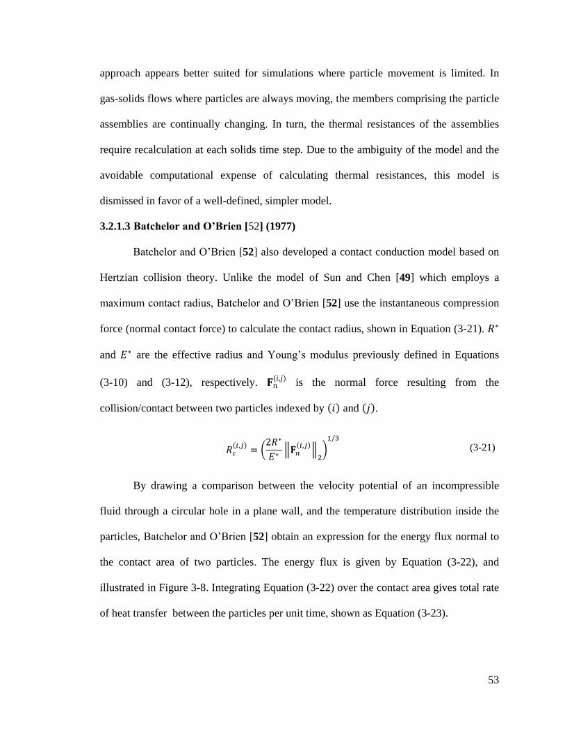
53

approach appears better suited for simulations where particle movement is limited. In

gas-solids flows where particles are always moving, the members comprising the particle

assemblies are continually changing. In turn, the thermal resistances of the assemblies

require recalculation at each solids time step. Due to the ambiguity of the model and the

avoidable computational expense of calculating thermal resistances, this model is

dismissed in favor of a well-defined, simpler model.

3.2.1.3 Batchelor and O’Brien [52] (1977)

Batchelor and O’Brien [52] also developed a contact conduction model based on

Hertzian collision theory. Unlike the model of Sun and Chen [49] which employs a

maximum contact radius, Batchelor and O’Brien [52] use the instantaneous compression

force (normal contact force) to calculate the contact radius, shown in Equation (3-21).

and are the effective radius and Young’s modulus previously defined in Equations

(3-10) and (3-12), respectively.

is the normal force resulting from the

collision/contact between two particles indexed by and .

(3-21)

By drawing a comparison between the velocity potential of an incompressible

fluid through a circular hole in a plane wall, and the temperature distribution inside the

particles, Batchelor and O’Brien [52] obtain an expression for the energy flux normal to

the contact area of two particles. The energy flux is given by Equation (3-22), and

illustrated in Figure 3-8. Integrating Equation (3-22) over the contact area gives total rate

of heat transfer between the particles per unit time, shown as Equation (3-23).

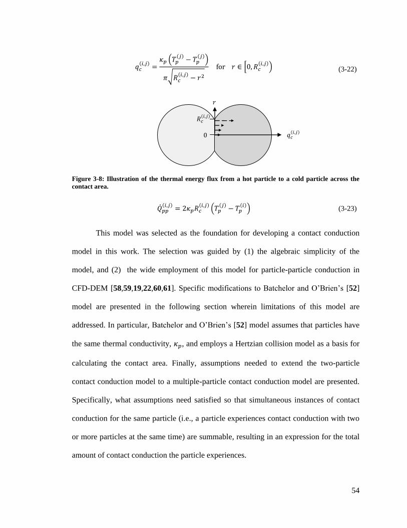
54

(3-22)

Figure 3-8: Illustration of the thermal energy flux from a hot particle to a cold particle across the

contact area.

(3-23)

This model was selected as the foundation for developing a contact conduction

model in this work. The selection was guided by (1) the algebraic simplicity of the

model, and (2) the wide employment of this model for particle-particle conduction in

CFD-DEM [58,59,19,22,60,61]. Specific modifications to Batchelor and O’Brien’s [52]

model are presented in the following section wherein limitations of this model are

addressed. In particular, Batchelor and O’Brien’s [52] model assumes that particles have

the same thermal conductivity, , and employs a Hertzian collision model as a basis for

calculating the contact area. Finally, assumptions needed to extend the two-particle

contact conduction model to a multiple-particle contact conduction model are presented.

Specifically, what assumptions need satisfied so that simultaneous instances of contact

conduction for the same particle (i.e., a particle experiences contact conduction with two

or more particles at the same time) are summable, resulting in an expression for the total

amount of contact conduction the particle experiences.

55

3.2.2 Modified Batchelor and O’Brien [52] two-particle contact conduction model

A constraint of Batchelor and O’Brien’s [52] contact conduction model is the

assumption that both particles have the same thermal conductivity, . This prohibits the

use of the model in systems where particle types, and in turn thermal conductivities of the

particles, may vary. Their model is extended in this work by defining an effective thermal

conductivity between two particles, shown in Equation (3-24). As defined, the smaller

thermal conductivity controls the rate of heat transfer across the contact area. This is

consistent with the thermal circuit concept put forward by Mills [47], whereby heat

transfer across a composite wall is limited by the material with the highest resistance to

conductive heat transfer. Likewise, Zhou, Yu, and Zulli [19] impose a similar

modification to Batchelor and O’Brien’s [52] model in their work.

(3-24)

In Batchelor and O’Brien’s [52] derivation, they employ a Hertzian collision

model to determine the area of contact through which heat may flow. In this effort, their

model is generalized further by using the geometric configuration of the two particles to

obtain the radius of their shared contact area. This approach results in a contact area

representative of the specific collision model employed by the DEM (e.g., Cundall and

Strack [44], Hertz [53], etc.), and promotes greater modeling consistency throughout the

CFD-DEM. Equation (3-25) defines the contact radius employed in this work. The

indices and are used to identify the particles by diameter size, specifically

and

; and, is the distance separating the

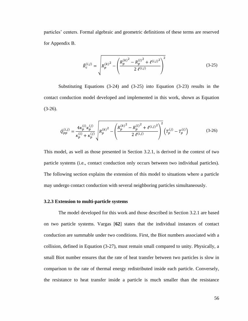
56

particles’ centers. Formal algebraic and geometric definitions of these terms are reserved

for Appendix B.

(3-25)

Substituting Equations (3-24) and (3-25) into Equation (3-23) results in the

contact conduction model developed and implemented in this work, shown as Equation

(3-26).

(3-26)

This model, as well as those presented in Section 3.2.1, is derived in the context of two

particle systems (i.e., contact conduction only occurs between two individual particles).

The following section explains the extension of this model to situations where a particle

may undergo contact conduction with several neighboring particles simultaneously.

3.2.3 Extension to multi-particle systems

The model developed for this work and those described in Section 3.2.1 are based

on two particle systems. Vargas [62] states that the individual instances of contact

conduction are summable under two conditions. First, the Biot numbers associated with a

collision, defined in Equation (3-27), must remain small compared to unity. Physically, a

small Biot number ensures that the rate of heat transfer between two particles is slow in

comparison to the rate of thermal energy redistributed inside each particle. Conversely,

the resistance to heat transfer inside a particle is much smaller than the resistance

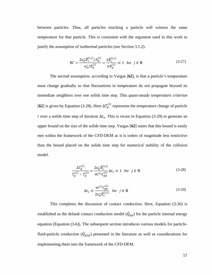
57

between particles. Thus, all particles touching a particle will witness the same

temperature for that particle. This is consistent with the argument used in this work to

justify the assumption of isothermal particles (see Section 3.1.2).

(3-27)

The second assumption, according to Vargas [62], is that a particle’s temperature

must change gradually so that fluctuations in temperature do not propagate beyond its

immediate neighbors over one solids time step. This quasi-steady temperature criterion

[62] is given by Equation (3-28). Here

represents the temperature change of particle

over a solids time step of duration . This is recast in Equation (3-29) to generate an

upper bound on the size of the solids time step. Vargas [62] states that this bound is easily

met within the framework of the CFD-DEM as it is orders of magnitude less restrictive

than the bound placed on the solids time step for numerical stability of the collision

model.

(3-28)

(3-29)

This completes the discussion of contact conduction. Here, Equation (3-26) is

established as the default contact conduction model ( ) for the particle internal energy

equation (Equation (3-6)). The subsequent section introduces various models for particle-

fluid-particle conduction ( ) presented in the literature as well as considerations for

implementing them into the framework of the CFD-DEM.

58

3.3 Particle-fluid-particle conduction

In addition to contact conduction, particles in close proximity to one another may

also transfer energy by conducting heat through the stagnant gas separating their surfaces.

Wen and Chang [63] suggest this form of conduction may contribute between 10-35% of

the total heat transferred among solids in some gas-solids systems.

3.3.1 Survey of particle-fluid-particle conduction models

This section begins by surveying several particle-fluid-particle conduction models

from the literature [16,63,64,65] along with various considerations that are needed to

implement each model in the selected CFD-DEM framework (i.e., MFIX-DEM). Rong

and Horio’s [16] model is selected as the basis for the particle-fluid-particle conduction

model developed in this work. Modifications to Rong and Horio’s [16] model are

discussed in Section 3.3.2.

3.3.1.1 Wen and Chang [63] (1967)

Wen and Chang [63] proposed a simple analytic model for heat transfer in gas-

solids systems operating at low temperatures and containing two types of particles (i.e.,

type A and type B particles). Particles of the same type are assumed identical in physical

and thermal properties as well as temperature. The authors hypothesize that heat

transferred from a particle’s surface primarily results from particle-gas convection and

particle-fluid-particle heat transfer. Contact conduction and radiative heat transfer are

assumed insignificant for their case (i.e., particulate fluidization at temperatures below

600°C). They conclude that the total flux of thermal energy across the surface of a type A

particle is given by Equation (3-30). The first component on the right hand side is the

59

flux due to particle-gas convection, while the second component is the result of particle-

fluid-particle conduction.

(3-30)

In Equation (3-30), is the convective heat transfer coefficient between the gas

and a type A particle, is the particle-particle heat transfer coefficient, and , , and

are the temperatures of the type A and B particles and gas, respectively. Wen and

Cheng [63] determined the particle-particle heat transfer coefficient through physical

experimentation.

The simplified analysis of heat transfer used to construct this model prevents it

from functioning as a general particle-fluid-particle conduction model. For example, the

authors hypothesize that contact conduction and radiative heat transfer are negligible,

limitations not imposed in the present work. In addition, enforcing the authors’

assumption that particles of the same type have the same temperature requires that each

Type A particle (or Type B particle) experience the same total heat flux. Otherwise, the

individual particles temperatures may diverge as the solutions to the internal energy

equations for the particles (i.e., Equation (3-6)) are advanced. Finally, expressions for the

particle-particle heat transfer coefficients are scarcely available and limit this model’s

validity to cases from which correlations are derived. As such, Wen and Chang’s [63]

model was not selected for this work.

3.3.1.2 Delvosalle and Vanderschuren [64] (1985)

Delvosalle and Vanderschuren [64] developed an analytic model for particle-

fluid-particle conduction by considering heat transfer between two isothermal particles in

a stagnant medium with negligible heat capacity. They hypothesize that for large

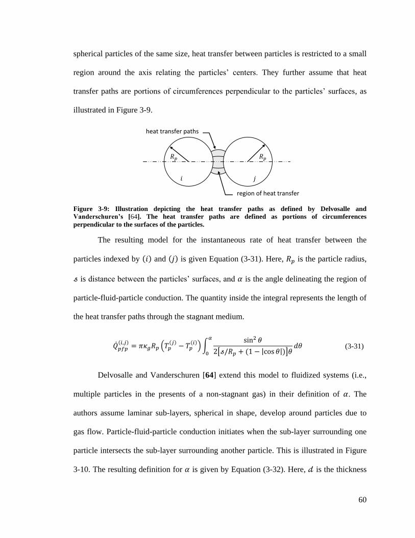
60

spherical particles of the same size, heat transfer between particles is restricted to a small

region around the axis relating the particles’ centers. They further assume that heat

transfer paths are portions of circumferences perpendicular to the particles’ surfaces, as

illustrated in Figure 3-9.

Figure 3-9: Illustration depicting the heat transfer paths as defined by Delvosalle and

Vanderschuren’s [64]. The heat transfer paths are defined as portions of circumferences

perpendicular to the surfaces of the particles.

The resulting model for the instantaneous rate of heat transfer between the

particles indexed by and is given Equation (3-31). Here, is the particle radius,

is distance between the particles’ surfaces, and is the angle delineating the region of

particle-fluid-particle conduction. The quantity inside the integral represents the length of

the heat transfer paths through the stagnant medium.

(3-31)

Delvosalle and Vanderschuren [64] extend this model to fluidized systems (i.e.,

multiple particles in the presents of a non-stagnant gas) in their definition of . The

authors assume laminar sub-layers, spherical in shape, develop around particles due to

gas flow. Particle-fluid-particle conduction initiates when the sub-layer surrounding one

particle intersects the sub-layer surrounding another particle. This is illustrated in Figure

3-10. The resulting definition for is given by Equation (3-32). Here, is the thickness

heat transfer paths

region of heat transfer

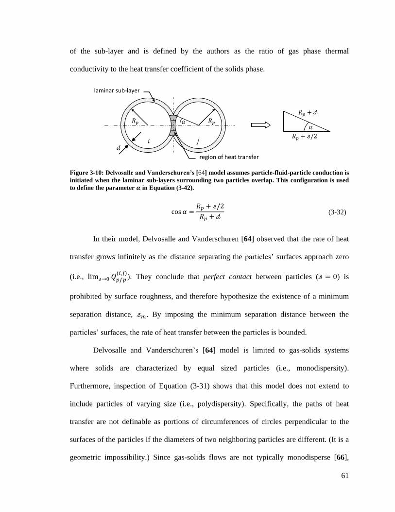
61

of the sub-layer and is defined by the authors as the ratio of gas phase thermal

conductivity to the heat transfer coefficient of the solids phase.

Figure 3-10: Delvosalle and Vanderschuren’s [64] model assumes particle-fluid-particle conduction is

initiated when the laminar sub-layers surrounding two particles overlap. This configuration is used

to define the parameter in Equation (3-42).

(3-32)

In their model, Delvosalle and Vanderschuren [64] observed that the rate of heat

transfer grows infinitely as the distance separating the particles’ surfaces approach zero

(i.e.,

). They conclude that perfect contact between particles ( ) is

prohibited by surface roughness, and therefore hypothesize the existence of a minimum

separation distance, . By imposing the minimum separation distance between the

particles’ surfaces, the rate of heat transfer between the particles is bounded.

Delvosalle and Vanderschuren’s [64] model is limited to gas-solids systems

where solids are characterized by equal sized particles (i.e., monodispersity).

Furthermore, inspection of Equation (3-31) shows that this model does not extend to

include particles of varying size (i.e., polydispersity). Specifically, the paths of heat

transfer are not definable as portions of circumferences of circles perpendicular to the

surfaces of the particles if the diameters of two neighboring particles are different. (It is a

geometric impossibility.) Since gas-solids flows are not typically monodisperse [66],

laminar sub-layer

region of heat transfer

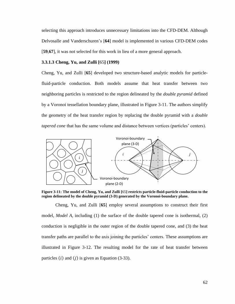
62

selecting this approach introduces unnecessary limitations into the CFD-DEM. Although

Delvosalle and Vanderschuren’s [64] model is implemented in various CFD-DEM codes

[59,67], it was not selected for this work in lieu of a more general approach.

3.3.1.3 Cheng, Yu, and Zulli [65] (1999)

Cheng, Yu, and Zulli [65] developed two structure-based analytic models for particle-

fluid-particle conduction. Both models assume that heat transfer between two

neighboring particles is restricted to the region delineated by the double pyramid defined

by a Voronoi tessellation boundary plane, illustrated in Figure 3-11. The authors simplify

the geometry of the heat transfer region by replacing the double pyramid with a double

tapered cone that has the same volume and distance between vertices (particles’ centers).

Figure 3-11: The model of Cheng, Yu, and Zulli [65] restricts particle-fluid-particle conduction to the

region delineated by the double pyramid (3-D) generated by the Voronoi-boundary plane.

Cheng, Yu, and Zulli [65] employ several assumptions to construct their first

model, Model A, including (1) the surface of the double tapered cone is isothermal, (2)

conduction is negligible in the outer region of the double tapered cone, and (3) the heat

transfer paths are parallel to the axis joining the particles’ centers. These assumptions are

illustrated in Figure 3-12. The resulting model for the rate of heat transfer between

particles and is given as Equation (3-33).

Voronoi-boundary

plane (3-D)

Voronoi-boundary

plane (2-D)

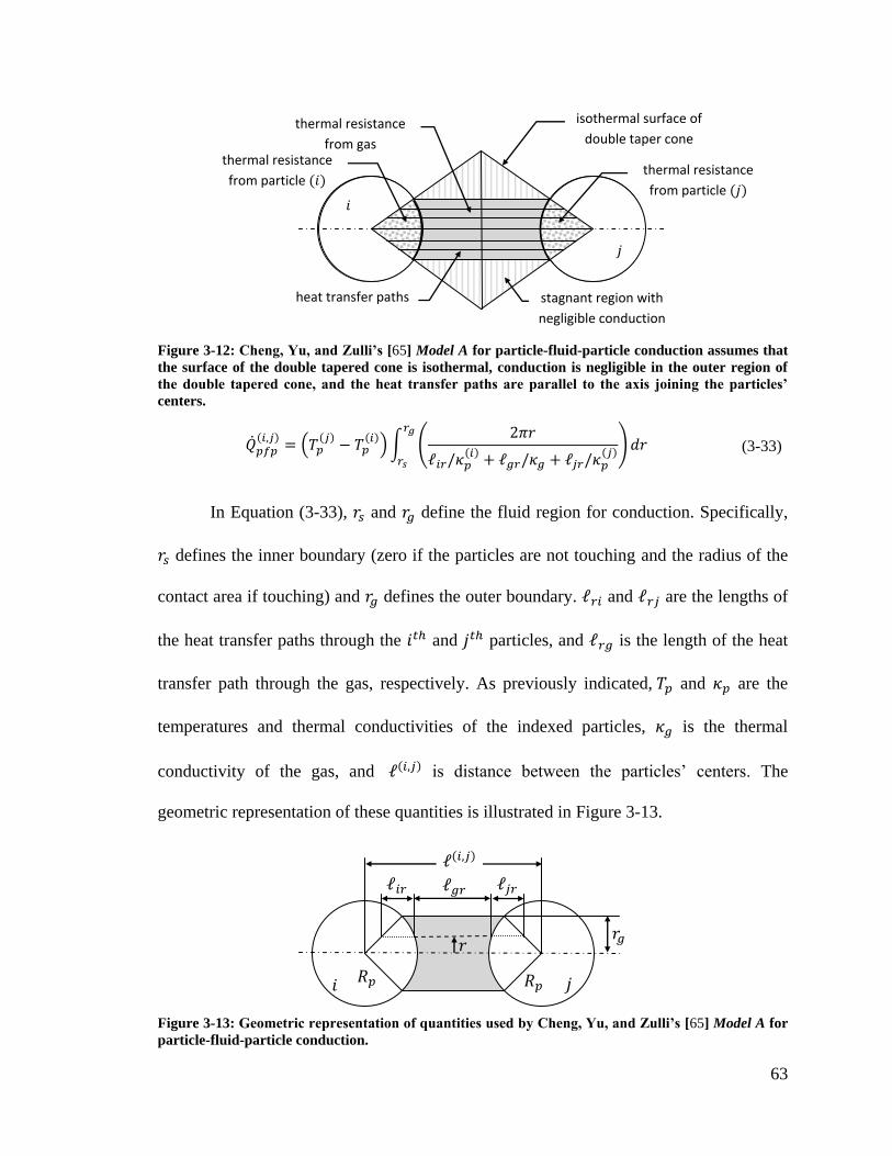
63

Figure 3-12: Cheng, Yu, and Zulli’s [65] Model A for particle-fluid-particle conduction assumes that

the surface of the double tapered cone is isothermal, conduction is negligible in the outer region of

the double tapered cone, and the heat transfer paths are parallel to the axis joining the particles’

centers.

(3-33)

In Equation (3-33), and define the fluid region for conduction. Specifically,

defines the inner boundary (zero if the particles are not touching and the radius of the

contact area if touching) and defines the outer boundary. and are the lengths of

the heat transfer paths through the and particles, and is the length of the heat

transfer path through the gas, respectively. As previously indicated, and are the

temperatures and thermal conductivities of the indexed particles, is the thermal

conductivity of the gas, and is distance between the particles’ centers. The

geometric representation of these quantities is illustrated in Figure 3-13.

Figure 3-13: Geometric representation of quantities used by Cheng, Yu, and Zulli’s [65] Model A for

particle-fluid-particle conduction.

stagnant region with

negligible conduction

heat transfer paths

isothermal surface of

double taper cone

thermal resistance

from particle thermal resistance

from particle

thermal resistance

from gas

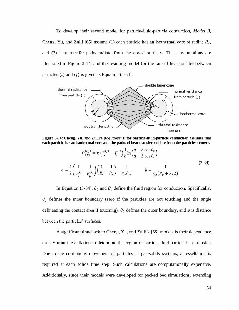
64

To develop their second model for particle-fluid-particle conduction, Model B,

Cheng, Yu, and Zulli [65] assume (1) each particle has an isothermal core of radius ,

and (2) heat transfer paths radiate from the cores’ surfaces. These assumptions are

illustrated in Figure 3-14, and the resulting model for the rate of heat transfer between

particles and is given as Equation (3-34).

Figure 3-14: Cheng, Yu, and Zulli’s [65] Model B for particle-fluid-particle conduction assumes that

each particle has an isothermal core and the paths of heat transfer radiate from the particles centers.

(3-34)

In Equation (3-34), and define the fluid region for conduction. Specifically,

defines the inner boundary (zero if the particles are not touching and the angle

delineating the contact area if touching), defines the outer boundary, and is distance

between the particles’ surfaces.

A significant drawback to Cheng, Yu, and Zulli’s [65] models is their dependence

on a Voronoi tessellation to determine the region of particle-fluid-particle heat transfer.

Due to the continuous movement of particles in gas-solids systems, a tessellation is

required at each solids time step. Such calculations are computationally expensive.

Additionally, since their models were developed for packed bed simulations, extending

double taper cone

heat transfer paths

isothermal core

thermal resistance

from particle thermal resistance

from particle

thermal resistance

from gas

65

them to fluidized systems may result in unphysical behavior. Specifically, particles that

are separated by large distances may share common Voronoi-boundaries, and in turn,

have the potential to engage in particle-fluid-particle heat transfer. Additional constraints

are needed to prevent this from occurring in the current model (i.e., a maximum distance

at which particle-fluid-particle ceases to occur). Finally, introducing models which

consider resistance to heat transfer through particles is contradictory to the assumption in

the present effort that particles are isothermal (see Section 3.1.2). Although a simplified

version of Model A is found in the CFD-DEM model of Zhou, Yu, and Zulli [19], neither

Model A nor Model B is selected for this work. This is due to the computational

complexity of the models and disagreement with the fundamental assumption employed

in this work of isothermal particles.

3.3.1.4 Rong and Horio [16] (1999)

Rong and Horio [16] introduced a particle-fluid-particle heat transfer model

similar to that of Delvosalle and Vanderschuren [64]. The authors hypothesize that (1)

each particle is surrounded by a gas layer with thickness , and (2) particle-particle

heat transfer initiates when the gas layer surrounding a particle intersects with the surface

of another particle. They further assume that (3) heat transfer occurs across paths parallel

to the axis joining the particles’ centers, and (4) a uniform gas layer, thick,

separates the particles’ surfaces as they collide. These assumptions are illustrated in

Figure 3-15. The resulting model is given in Equation (3-35).

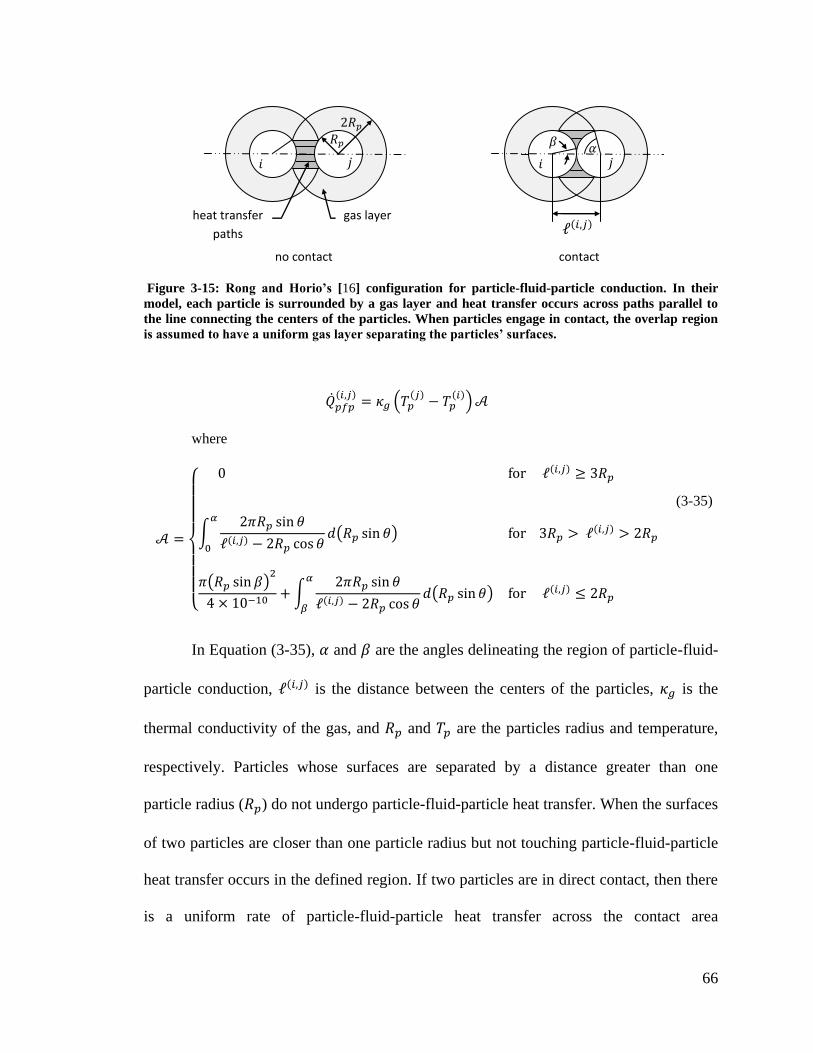
66

Figure 3-15: Rong and Horio’s [16] configuration for particle-fluid-particle conduction. In their

model, each particle is surrounded by a gas layer and heat transfer occurs across paths parallel to

the line connecting the centers of the particles. When particles engage in contact, the overlap region

is assumed to have a uniform gas layer separating the particles’ surfaces.

where

(3-35)

In Equation (3-35), and are the angles delineating the region of particle-fluid-

particle conduction, is the distance between the centers of the particles, is the

thermal conductivity of the gas, and and are the particles radius and temperature,

respectively. Particles whose surfaces are separated by a distance greater than one

particle radius ( ) do not undergo particle-fluid-particle heat transfer. When the surfaces

of two particles are closer than one particle radius but not touching particle-fluid-particle

heat transfer occurs in the defined region. If two particles are in direct contact, then there

is a uniform rate of particle-fluid-particle heat transfer across the contact area

heat transfer

paths

gas layer

no contact contact

67

as particle-fluid-particle heat transfer occurs around the interface of the

contact area.

This model was selected as the foundation for the particle-fluid-particle model

developed in this work. Like the model proposed by Delvosalle and Vanderschuren [64],

Rong and Horio’s [16] approach is valid only for particles of equal diameter. However,

unlike Delvosalle and Vanderschuren’s [64] model, the model proposed by Rong and

Horio [16] extends to particles of different sizes by modifying several geometric

definitions. The extension is possible because Rong and Horio [16] assume that heat

transfer paths are parallel to the axis joining the particles’ centers as opposed to the arc

structures used by Delvosalle and Vanderschuren [64]. The following section presents the

extension of Rong and Horio’s [16] model to include particles of different sizes.

3.3.2 Modified Rong and Horio [16] particle-fluid-particle conduction model

As previously noted, Rong and Horio’s [16] model for particle-fluid-particle

conduction was developed in the context of equal size particles. Extending their model to

particles of different size requires a standard point of reference to develop a consistent

definition for the particle-fluid-particle region. This specification is satisfied by

delineating the outer region of particle-fluid-particle heat transfer by the intersection of

the gas layer surrounding the larger particle with the surface of the smaller particle. This

is expressed by Equation (3-36) and illustrated in Figure 3-16. Here, the indices and

identify the particles by size, specifically

and

, and is the thickness of the gas layer.

is similar to in

Equation (3-35) in that it delineates the upper bound on the region of particle-fluid-

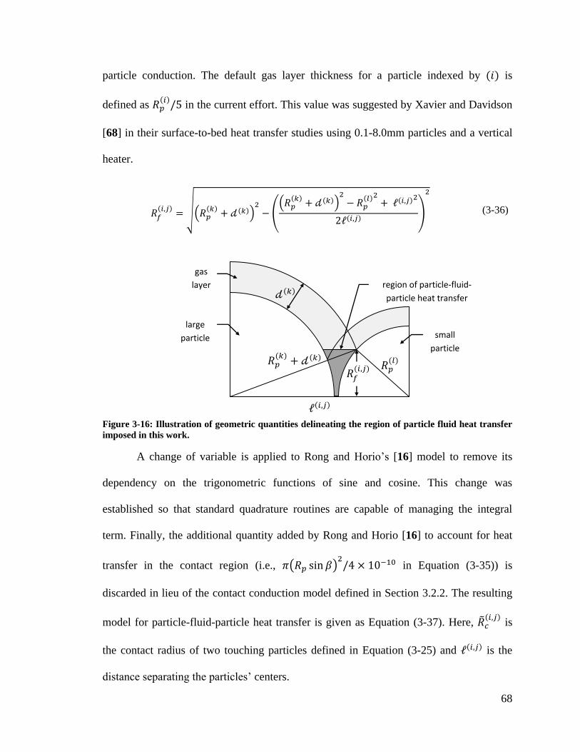
68

particle conduction. The default gas layer thickness for a particle indexed by is

defined as in the current effort. This value was suggested by Xavier and Davidson

[68] in their surface-to-bed heat transfer studies using 0.1-8.0mm particles and a vertical

heater.

(3-36)

Figure 3-16: Illustration of geometric quantities delineating the region of particle fluid heat transfer

imposed in this work.

A change of variable is applied to Rong and Horio’s [16] model to remove its

dependency on the trigonometric functions of sine and cosine. This change was

established so that standard quadrature routines are capable of managing the integral

term. Finally, the additional quantity added by Rong and Horio [16] to account for heat

transfer in the contact region (i.e., in Equation (3-35)) is

discarded in lieu of the contact conduction model defined in Section 3.2.2. The resulting

model for particle-fluid-particle heat transfer is given as Equation (3-37). Here,

is

the contact radius of two touching particles defined in Equation (3-25) and is the

distance separating the particles’ centers.

small

particle

large

particle

gas

layer

region of particle-fluid-

particle heat transfer

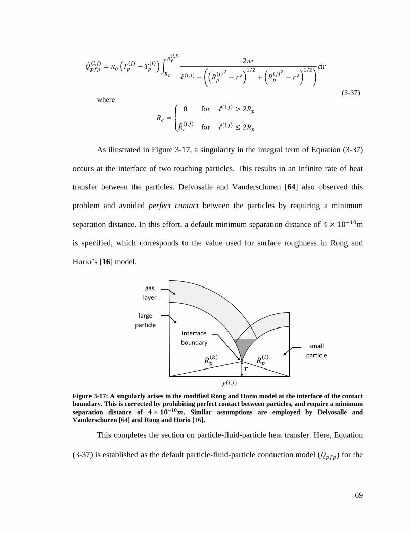
69

where

(3-37)

As illustrated in Figure 3-17, a singularity in the integral term of Equation (3-37)

occurs at the interface of two touching particles. This results in an infinite rate of heat

transfer between the particles. Delvosalle and Vanderschuren [64] also observed this

problem and avoided perfect contact between the particles by requiring a minimum

separation distance. In this effort, a default minimum separation distance of m

is specified, which corresponds to the value used for surface roughness in Rong and

Horio’s [16] model.

Figure 3-17: A singularly arises in the modified Rong and Horio model at the interface of the contact

boundary. This is corrected by prohibiting perfect contact between particles, and require a minimum

separation distance of . Similar assumptions are employed by Delvosalle and

Vanderschuren [64] and Rong and Horio [16].

This completes the section on particle-fluid-particle heat transfer. Here, Equation

(3-37) is established as the default particle-fluid-particle conduction model ( ) for the

small

particle

large

particle

gas

layer

interface

boundary

70

particle internal energy equation (Equation (3-6)). The following section considers

particle-gas convective heat transfer ( ) in gas-solids systems.

3.4 Particle-gas convection

Recall, convection is defined in this effort as heat transfer between a particle and

the surrounding gas resulting from differences in temperature and velocity. This section

introduces Newton’s law of cooling for modeling convection, and briefly discusses the

connection between the convective heat transfer coefficient and dimensionless Nusselt

number. The Ranz and Marshall [69] correlation for the Nusselt number, selected as the

default correlation in this work, is presented.

3.4.1 Background of particle-gas convection

Heat transfer between a particle and gas is assumed in this work to follow

Newton's law of cooling. Newton's law of cooling, shown as Equation (3-38),

hypothesizes that the rate of heat transfer between two objects is proportional their

temperature difference. The constant of proportionality for convective heat transfer

between a particle and gas often is given as the combination of a convective heat transfer

coefficient ( ) and the surface area of the particle ( ). Therefore, the rate of

convective heat transfer between a single particle and moving gas is given by Equation

(3-39), where is the particle's temperature, and is the average temperature of the gas

surrounding the particle.

(3-38)

(3-39)

71

The convective heat transfer coefficient is commonly modeled by the

dimensionless Nusselt number which expresses the ratio of total convective heat transfer

to conductive heat transfer. The Nusselt number for a spherical particle is shown in

Equation (3-40), where is the particle’s radius and is the thermal conductivity of

the gas phase. Note that the Nusselt number's definition is similar that of the Biot number

presented in Equation (3-4). However, the Nusselt number's definition uses the thermal

conductivity of the fluid as opposed to the solid.

(3-40)

A large number of experimental correlations for the Nusselt number are available

in the literature [69,70,71,72,73]. Typically, correlations are reported in a format similar

to that presented in Equation (3-41) where , , , and are fitted empirical constants,

and and are the dimensionless Reynolds and Prandtl numbers, respectively. The

Reynolds number, defined in Equation (3-42), is the ratio of inertial forces and viscous

forces in the fluid. The Prandtl number, given by Equation (3-43), is the ratio of

momentum and thermal diffusivity in the fluid. In these equations, , , , , ,

and are the density, void fraction, thermal conductivity, specific heat, viscosity, and

velocity of the gas, respectively. and are the radius and velocity of the particle.

(3-41)

(3-42)

(3-43)

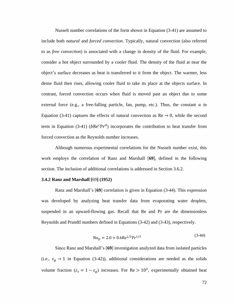
72

Nusselt number correlations of the form shown in Equation (3-41) are assumed to

include both natural and forced convection. Typically, natural convection (also referred

to as free convection) is associated with a change in density of the fluid. For example,

consider a hot object surrounded by a cooler fluid. The density of the fluid at near the

object’s surface decreases as heat is transferred to it from the object. The warmer, less

dense fluid then rises, allowing cooler fluid to take its place at the objects surface. In

contrast, forced convection occurs when fluid is moved past an object due to some

external force (e.g., a free-falling particle, fan, pump, etc.). Thus, the constant in

Equation (3-41) captures the effects of natural convection as , while the second

term in Equation (3-41) ( ) incorporates the contribution to heat transfer from

forced convection as the Reynolds number increases.

Although numerous experimental correlations for the Nusselt number exist, this

work employs the correlation of Ranz and Marshall [69], defined in the following

section. The inclusion of additional correlations is addressed in Section 3.6.2.

3.4.2 Ranz and Marshall [69] (1952)

Ranz and Marshall’s [69] correlation is given in Equation (3-44). This expression

was developed by analyzing heat transfer data from evaporating water droplets,

suspended in an upward-flowing gas. Recall that and are the dimensionless

Reynolds and Prandtl numbers defined in Equations (3-42) and (3-43), respectively.

(3-44)

Since Ranz and Marshall’s [69] investigation analyzed data from isolated particles

(i.e., in Equation (3-42)), additional considerations are needed as the solids

volume fraction ( ) increases. For , experimentally obtained heat

73

transfer data from fluidized beds was shown to agree reasonably well with Equation

(3-44). However, as the Reynolds number decreases ( ), Equation (3-44) is shown

to over predict the heat transfer coefficient for a bed of particles [74]. Specifically, as the

Reynolds number decreases, observed values for the Nusselt number for the bed drop

below two, the theoretical minimum given by Equation (3-44) as . It is

hypothesized that this is a result of reduced particle-gas contact as particles in a bed move

closer together [74]. No bounds on void fraction were found in the literature indicating an

acceptable rage in which this model is applicable. Additionally, no bounds for the

Reynolds and Prandtl numbers were provided by Ranz and Marshall [69], but several

recommendations are found in the literature. Fan and Zhu [29] suggest that Equation

(3-44) is applicable for and encompassing most gas-solids flows. Li

and Mason [17] claim Equation (3-44) provides acceptable results for , while

Mankad, Nixon, and Fryer [75] suggest it only applicable for .

Ranz and Marshall’s [69] correlation is employed in numerous CFD-DEM models

[2,16,17,21,76] as well as a variation found in [18] (i.e., ).

Likewise, Equation (3-44) was selected as the default correlation for this work. The

consideration to include additional correlations in the future is addressed in Section 3.6.2.

This completes the discussion on particle-gas convective heat transfer. Here, Equation

(3-39) is established as the convective heat transfer model ( ) for the particle internal

energy equation (Equation (3-6)). Ranz and Marshall's [69] Nusselt number correlation

(Equation (3-44)) was selected as the default closure model for the heat transfer

coefficient ( ) in Equation (3-39). The following section introduces particle-

environment radiative heat transfer ( ) in gas-solids systems.

74

3.5 Particle-particle radiation

Radiative heat transfer occurs between the surfaces of solids [77] as well as an

object’s surface and the fluid surrounding it. Specifically, radiative heat transfer in gas-

solids systems may occur between the particles and walls, individual/groups of particles,

and the particles and gas. Presently, MFIX-DEM operates with the assumption that

system walls are adiabatic (i.e., perfectly insulated so that no thermal energy enters or

leaves the system through the walls). As a result, radiative heat transfer between particles

and walls is not considered. Information concerning particle-wall heat transfer is found in

references [29,78,79]. Additionally, this work assumes that the gas phase is perfectly

transparent (i.e., the gas offers no resistance or contribution to radiative heat transfer).

Therefore, particle-gas radiative heat transfer is also not considered. Information

concerning particle-gas radiative heat transfer is provided in references [47,80]. Finally,

particle-particle radiative heat transfer is commonly omitted from CFD-DEM heat

transfer models [17,21,51,59,60,61,63,67,76,81] due to its negligible contribution to

overall heat transfer at temperatures below [63]. However, as temperatures

increase, the importance of particle-environment radiation also increases [19,78]. Since a

goal of this work is to construct a comprehensive heat transfer model for the CFD-DEM,

particle-particle radiative heat transfer is included for completeness. The negligible effect

of radiative heat transfer at moderate temperatures is addressed in the implementation

discussion.

This section continues by briefly describing radiative heat transfer, whereas the

interested reader is directed to references [47,82] for a thorough review of the topic. The

radiative heat transfer model employed in various CFD-DEM models is presented.

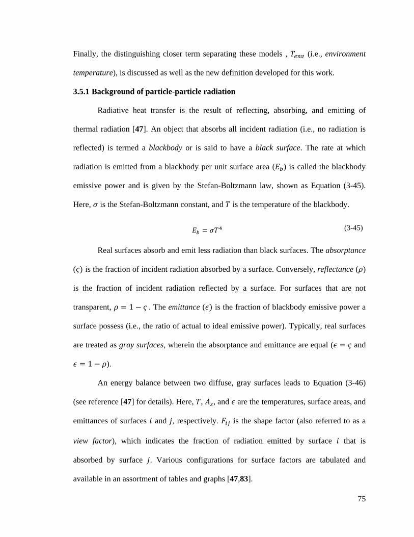
75

Finally, the distinguishing closer term separating these models , (i.e., environment

temperature), is discussed as well as the new definition developed for this work.

3.5.1 Background of particle-particle radiation

Radiative heat transfer is the result of reflecting, absorbing, and emitting of

thermal radiation [47]. An object that absorbs all incident radiation (i.e., no radiation is

reflected) is termed a blackbody or is said to have a black surface. The rate at which

radiation is emitted from a blackbody per unit surface area ( ) is called the blackbody

emissive power and is given by the Stefan-Boltzmann law, shown as Equation (3-45).

Here, is the Stefan-Boltzmann constant, and is the temperature of the blackbody.

(3-45)

Real surfaces absorb and emit less radiation than black surfaces. The absorptance

( is the fraction of incident radiation absorbed by a surface. Conversely, reflectance ( )

is the fraction of incident radiation reflected by a surface. For surfaces that are not

transparent, . The emittance ( is the fraction of blackbody emissive power a

surface possess (i.e., the ratio of actual to ideal emissive power). Typically, real surfaces

are treated as gray surfaces, wherein the absorptance and emittance are equal ( and

).

An energy balance between two diffuse, gray surfaces leads to Equation (3-46)

(see reference [47] for details). Here, , , and are the temperatures, surface areas, and

emittances of surfaces and , respectively. is the shape factor (also referred to as a

view factor), which indicates the fraction of radiation emitted by surface that is

absorbed by surface . Various configurations for surface factors are tabulated and

available in an assortment of tables and graphs [47,83].

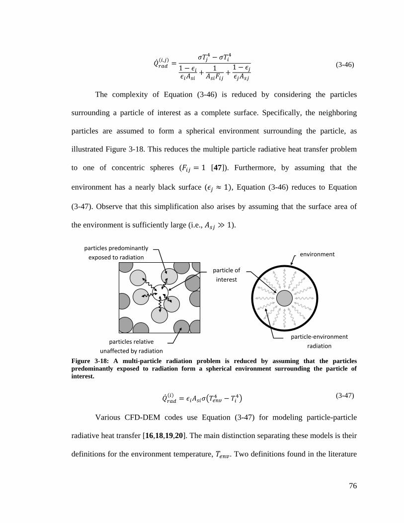
76

(3-46)

The complexity of Equation (3-46) is reduced by considering the particles

surrounding a particle of interest as a complete surface. Specifically, the neighboring

particles are assumed to form a spherical environment surrounding the particle, as

illustrated Figure 3-18. This reduces the multiple particle radiative heat transfer problem

to one of concentric spheres ( [47]). Furthermore, by assuming that the

environment has a nearly black surface ( , Equation (3-46) reduces to Equation

(3-47). Observe that this simplification also arises by assuming that the surface area of

the environment is sufficiently large (i.e., ).

Figure 3-18: A multi-particle radiation problem is reduced by assuming that the particles

predominantly exposed to radiation form a spherical environment surrounding the particle of

interest.

(3-47)

Various CFD-DEM codes use Equation (3-47) for modeling particle-particle

radiative heat transfer [16,18,19,20]. The main distinction separating these models is their

definitions for the environment temperature, . Two definitions found in the literature

environment

particles relative

unaffected by radiation

particles predominantly

exposed to radiation

particle of

interest

particle-environment

radiation

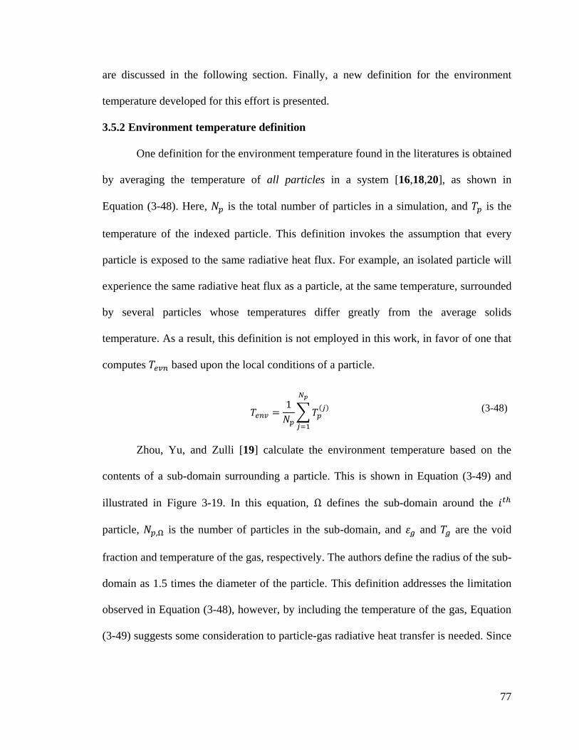
77

are discussed in the following section. Finally, a new definition for the environment

temperature developed for this effort is presented.

3.5.2 Environment temperature definition

One definition for the environment temperature found in the literatures is obtained

by averaging the temperature of all particles in a system [16,18,20], as shown in

Equation (3-48). Here, is the total number of particles in a simulation, and is the

temperature of the indexed particle. This definition invokes the assumption that every

particle is exposed to the same radiative heat flux. For example, an isolated particle will

experience the same radiative heat flux as a particle, at the same temperature, surrounded

by several particles whose temperatures differ greatly from the average solids

temperature. As a result, this definition is not employed in this work, in favor of one that

computes based upon the local conditions of a particle.

(3-48)

Zhou, Yu, and Zulli [19] calculate the environment temperature based on the

contents of a sub-domain surrounding a particle. This is shown in Equation (3-49) and

illustrated in Figure 3-19. In this equation, defines the sub-domain around the

particle, is the number of particles in the sub-domain, and and are the void

fraction and temperature of the gas, respectively. The authors define the radius of the sub-

domain as 1.5 times the diameter of the particle. This definition addresses the limitation

observed in Equation (3-48), however, by including the temperature of the gas, Equation

(3-49) suggests some consideration to particle-gas radiative heat transfer is needed. Since

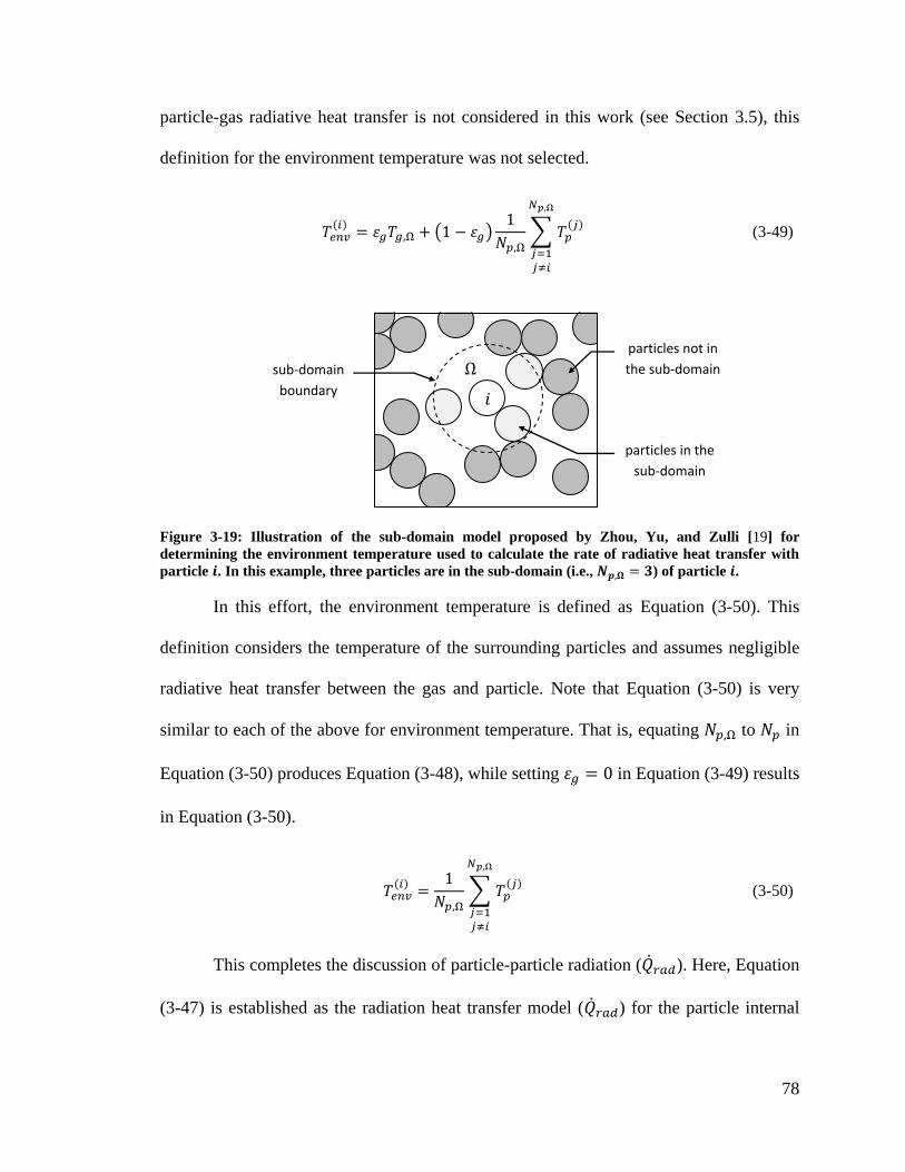
78

particle-gas radiative heat transfer is not considered in this work (see Section 3.5), this

definition for the environment temperature was not selected.

(3-49)

Figure 3-19: Illustration of the sub-domain model proposed by Zhou, Yu, and Zulli [19] for

determining the environment temperature used to calculate the rate of radiative heat transfer with

particle . In this example, three particles are in the sub-domain (i.e., ) of particle .

In this effort, the environment temperature is defined as Equation (3-50). This

definition considers the temperature of the surrounding particles and assumes negligible

radiative heat transfer between the gas and particle. Note that Equation (3-50) is very

similar to each of the above for environment temperature. That is, equating to in

Equation (3-50) produces Equation (3-48), while setting in Equation (3-49) results

in Equation (3-50).

(3-50)

This completes the discussion of particle-particle radiation ( ). Here, Equation

(3-47) is established as the radiation heat transfer model ( ) for the particle internal

particles not in

the sub-domain

particles in the

sub-domain

sub-domain

boundary

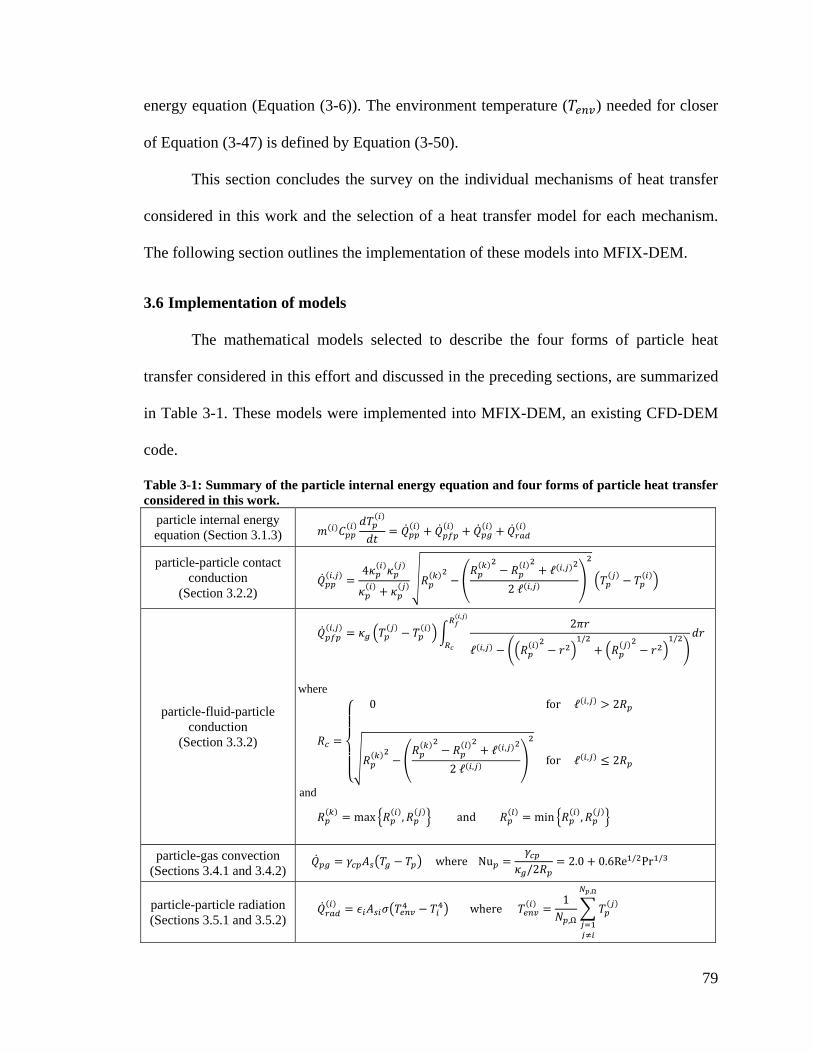
79

energy equation (Equation (3-6)). The environment temperature ( ) needed for closer

of Equation (3-47) is defined by Equation (3-50).

This section concludes the survey on the individual mechanisms of heat transfer

considered in this work and the selection of a heat transfer model for each mechanism.

The following section outlines the implementation of these models into MFIX-DEM.

3.6 Implementation of models

The mathematical models selected to describe the four forms of particle heat

transfer considered in this effort and discussed in the preceding sections, are summarized

in Table 3-1. These models were implemented into MFIX-DEM, an existing CFD-DEM

code.

Table 3-1: Summary of the particle internal energy equation and four forms of particle heat transfer

considered in this work.

particle internal energy

equation (Section 3.1.3)

particle-particle contact

conduction

(Section 3.2.2)

particle-fluid-particle

conduction

(Section 3.3.2)

where

and

particle-gas convection

(Sections 3.4.1 and 3.4.2)

particle-particle radiation

(Sections 3.5.1 and 3.5.2)

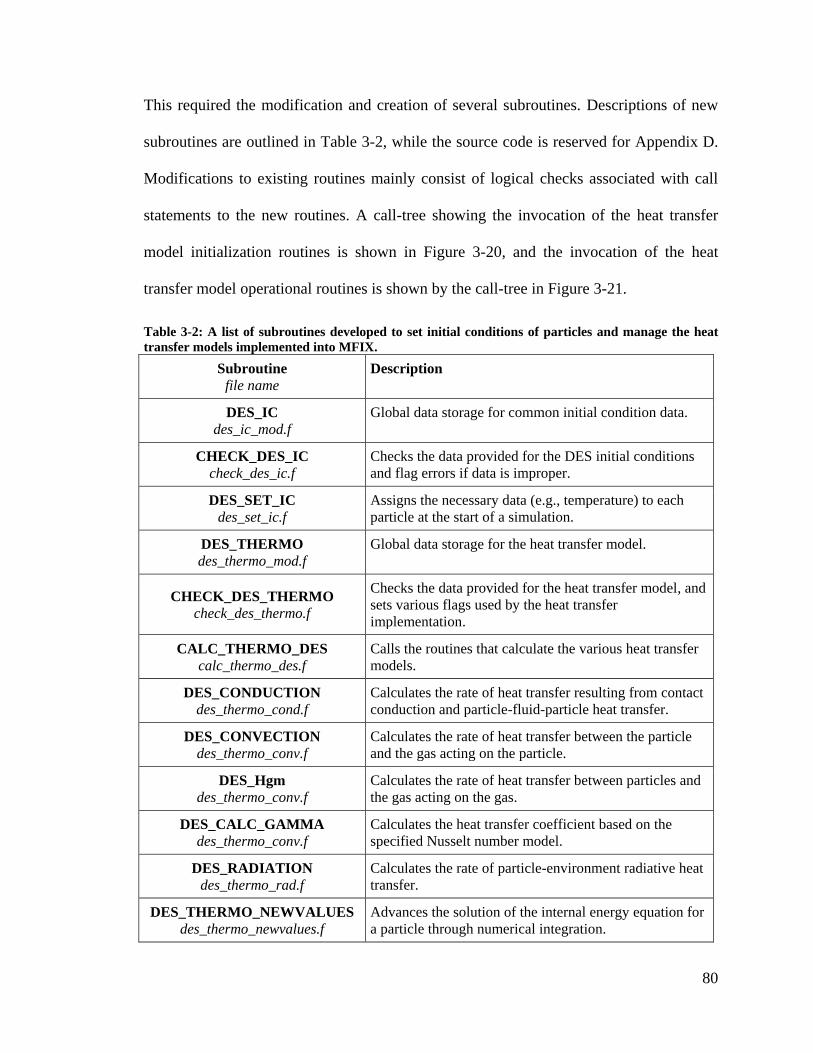
80

This required the modification and creation of several subroutines. Descriptions of new

subroutines are outlined in Table 3-2, while the source code is reserved for Appendix D.

Modifications to existing routines mainly consist of logical checks associated with call

statements to the new routines. A call-tree showing the invocation of the heat transfer

model initialization routines is shown in Figure 3-20, and the invocation of the heat

transfer model operational routines is shown by the call-tree in Figure 3-21.

Table 3-2: A list of subroutines developed to set initial conditions of particles and manage the heat

transfer models implemented into MFIX.

Subroutine

file name

Description

DES_IC

des_ic_mod.f

Global data storage for common initial condition data.

CHECK_DES_IC

check_des_ic.f

Checks the data provided for the DES initial conditions

and flag errors if data is improper.

DES_SET_IC

des_set_ic.f

Assigns the necessary data (e.g., temperature) to each

particle at the start of a simulation.

DES_THERMO

des_thermo_mod.f

Global data storage for the heat transfer model.

CHECK_DES_THERMO

check_des_thermo.f

Checks the data provided for the heat transfer model, and

sets various flags used by the heat transfer

implementation.

CALC_THERMO_DES

calc_thermo_des.f

Calls the routines that calculate the various heat transfer

models.

DES_CONDUCTION

des_thermo_cond.f

Calculates the rate of heat transfer resulting from contact

conduction and particle-fluid-particle heat transfer.

DES_CONVECTION

des_thermo_conv.f

Calculates the rate of heat transfer between the particle

and the gas acting on the particle.

DES_Hgm

des_thermo_conv.f

Calculates the rate of heat transfer between particles and

the gas acting on the gas.

DES_CALC_GAMMA

des_thermo_conv.f

Calculates the heat transfer coefficient based on the

specified Nusselt number model.

DES_RADIATION

des_thermo_rad.f

Calculates the rate of particle-environment radiative heat

transfer.

DES_THERMO_NEWVALUES

des_thermo_newvalues.f

Advances the solution of the internal energy equation for

a particle through numerical integration.

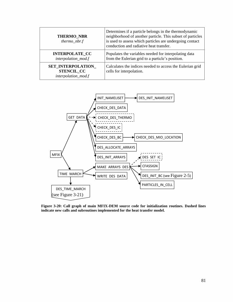
81

THERMO_NBR

thermo_nbr.f

Determines if a particle belongs in the thermodynamic

neighborhood of another particle. This subset of particles

is used to assess which particles are undergoing contact

conduction and radiative heat transfer.

INTERPOLATE_CC

interpolation_mod.f

Populates the variables needed for interpolating data

from the Eulerian grid to a particle’s position.

SET_INTERPOLATION_

STENCIL_CC

interpolation_mod.f

Calculates the indices needed to access the Eulerian grid

cells for interpolation.

Figure 3-20: Call graph of main MFIX-DEM source code for initialization routines. Dashed lines

indicate new calls and subroutines implemented for the heat transfer model.

MFIX

GET_DATA


DES_ALLOCATE_ARRAYS

DES_INIT_ARRAYS

CHECK_DES_DATA

CHECK_DES_THERMO

TIME_MARCH

MAKE_ARRAYS_DES

WRITE_DES_DATA

DES_SET_IC

DES_TIME_MARCH

(see Figure 3-21)

)

CHECK_DES_IC

CHECK_DES_BC CHECK_DES_MIO_LOCATION

DES_INIT_BC (see Figure 2-5)

PARTICLES_IN_CELL

CFASSIGN

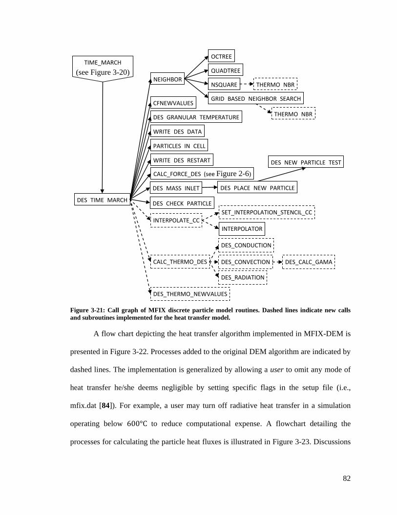
82

Figure 3-21: Call graph of MFIX discrete particle model routines. Dashed lines indicate new calls

and subroutines implemented for the heat transfer model.

A flow chart depicting the heat transfer algorithm implemented in MFIX-DEM is

presented in Figure 3-22. Processes added to the original DEM algorithm are indicated by

dashed lines. The implementation is generalized by allowing a user to omit any mode of

heat transfer he/she deems negligible by setting specific flags in the setup file (i.e.,

mfix.dat [84]). For example, a user may turn off radiative heat transfer in a simulation

operating below to reduce computational expense. A flowchart detailing the

processes for calculating the particle heat fluxes is illustrated in Figure 3-23. Discussions

DES_TIME_MARCH

NEIGHBOR

CFNEWVALUES


WRITE_DES_DATA

PARTICLES_IN_CELL

WRITE_DES_RESTART

CALC_FORCE_DES (see Figure 2-6)

TIME_MARCH

(see Figure 3-20)

INTERPOLATE_CC SET_INTERPOLATION_STENCIL_CC

INTERPOLATOR

CALC_THERMO_DES


DES_CONVECTION

DES_CONDUCTION

DES_RADIATION

NSQUARE


QUADTREE

OCTREE

THERMO_NBR

THERMO_NBR

DES_CALC_GAMA

DES_MASS_INLET

DES_CHECK_PARTICLE



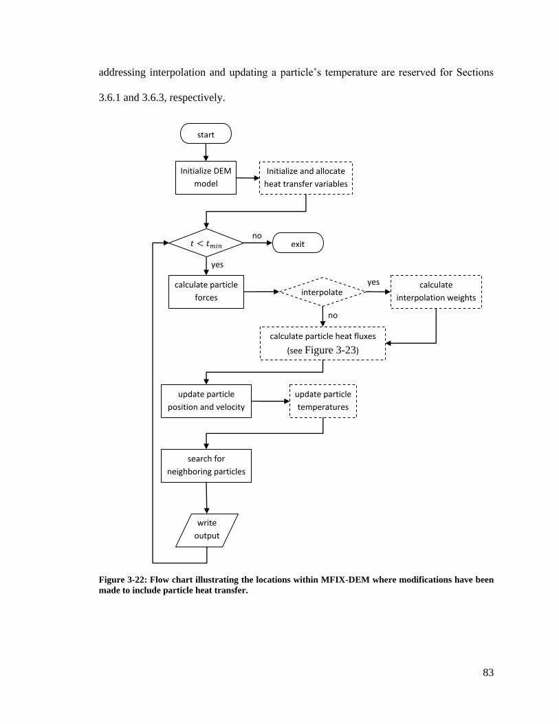
83

addressing interpolation and updating a particle’s temperature are reserved for Sections

3.6.1 and 3.6.3, respectively.


made to include particle heat transfer.

Initialize DEM

model

Initialize and allocate

heat transfer variables

calculate particle

forces

update particle


exit

start

no

yes

update particle

temperatures

search for


calculate particle heat fluxes

(see Figure 3-23)

interpolate

no

calculate

interpolation weights

yes

write

output

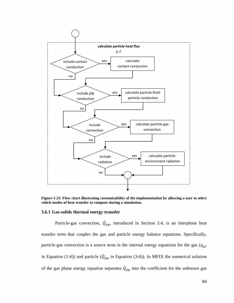
84

Figure 3-23: Flow chart illustrating customizability of the implementation by allowing a user to select

which modes of heat transfer to compute during a simulation.

3.6.1 Gas-solids thermal energy transfer

Particle-gas convection, , introduced in Section 3.4, is an interphase heat

transfer term that couples the gas and particle energy balance equations. Specifically,

particle-gas convection is a source term in the internal energy equations for the gas (

in Equation (1-6)) and particle ( in Equation (3-6)). In MFIX the numerical solution

of the gas phase energy equation separates into the coefficient for the unknown gas

include contact

conduction

calculate

contact conduction

no

include pfp

conduction

calculate particle-fluid-

particle conduction

no

include

convection

calculate particle-gas

convection

no

include

radiation

calculate particle-

environment radiation

yes

yes

yes

yes

no

calculate particle heat flux

(c.f.

Figure 3-22)

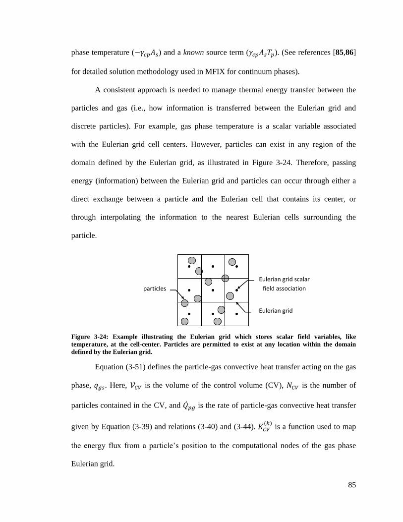
85

phase temperature ( ) and a known source term ( ). (See references [85,86]

for detailed solution methodology used in MFIX for continuum phases).

A consistent approach is needed to manage thermal energy transfer between the

particles and gas (i.e., how information is transferred between the Eulerian grid and

discrete particles). For example, gas phase temperature is a scalar variable associated

with the Eulerian grid cell centers. However, particles can exist in any region of the

domain defined by the Eulerian grid, as illustrated in Figure 3-24. Therefore, passing

energy (information) between the Eulerian grid and particles can occur through either a

direct exchange between a particle and the Eulerian cell that contains its center, or

through interpolating the information to the nearest Eulerian cells surrounding the

particle.

Figure 3-24: Example illustrating the Eulerian grid which stores scalar field variables, like

temperature, at the cell-center. Particles are permitted to exist at any location within the domain

defined by the Eulerian grid.

Equation (3-51) defines the particle-gas convective heat transfer acting on the gas

phase, . Here, is the volume of the control volume (CV), is the number of

particles contained in the CV, and is the rate of particle-gas convective heat transfer

given by Equation (3-39) and relations (3-40) and (3-44).

is a function used to map

the energy flux from a particle’s position to the computational nodes of the gas phase

Eulerian grid.

Eulerian grid

Eulerian grid scalar

field association particles

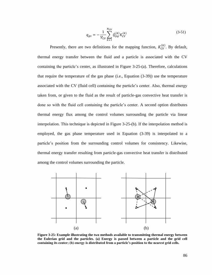
86

(3-51)

Presently, there are two definitions for the mapping function,

. By default,

thermal energy transfer between the fluid and a particle is associated with the CV

containing the particle’s center, as illustrated in Figure 3-25-(a). Therefore, calculations

that require the temperature of the gas phase (i.e., Equation (3-39)) use the temperature

associated with the CV (fluid cell) containing the particle’s center. Also, thermal energy

taken from, or given to the fluid as the result of particle-gas convective heat transfer is

done so with the fluid cell containing the particle’s center. A second option distributes

thermal energy flux among the control volumes surrounding the particle via linear

interpolation. This technique is depicted in Figure 3-25-(b). If the interpolation method is

employed, the gas phase temperature used in Equation (3-39) is interpolated to a

particle’s position from the surrounding control volumes for consistency. Likewise,

thermal energy transfer resulting from particle-gas convective heat transfer is distributed

among the control volumes surrounding the particle.

Figure 3-25: Example illustrating the two methods available to transmitting thermal energy between

the Eulerian grid and the particles. (a) Energy is passed between a particle and the grid cell

containing its center; (b) energy is distributed from a particle’s position to the nearest grid cells.

(a) (b)

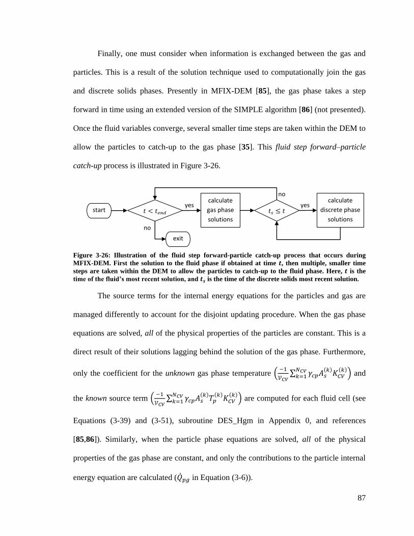
87

Finally, one must consider when information is exchanged between the gas and

particles. This is a result of the solution technique used to computationally join the gas

and discrete solids phases. Presently in MFIX-DEM [85], the gas phase takes a step

forward in time using an extended version of the SIMPLE algorithm [86] (not presented).

Once the fluid variables converge, several smaller time steps are taken within the DEM to

allow the particles to catch-up to the gas phase [35]. This fluid step forward–particle

catch-up process is illustrated in Figure 3-26.

Figure 3-26: Illustration of the fluid step forward-particle catch-up process that occurs during

MFIX-DEM. First the solution to the fluid phase if obtained at time , then multiple, smaller time

steps are taken within the DEM to allow the particles to catch-up to the fluid phase. Here, is the

time of the fluid’s most recent solution, and is the time of the discrete solids most recent solution.

The source terms for the internal energy equations for the particles and gas are

managed differently to account for the disjoint updating procedure. When the gas phase

equations are solved, all of the physical properties of the particles are constant. This is a

direct result of their solutions lagging behind the solution of the gas phase. Furthermore,

only the coefficient for the unknown gas phase temperature

and

the known source term

are computed for each fluid cell (see

Equations (3-39) and (3-51), subroutine DES_Hgm in Appendix 0, and references

[85,86]). Similarly, when the particle phase equations are solved, all of the physical

properties of the gas phase are constant, and only the contributions to the particle internal

energy equation are calculated ( in Equation (3-6)).

calculate

gas phase

solutions

exit

start yes

calculate

discrete phase

solutions no

yes

no

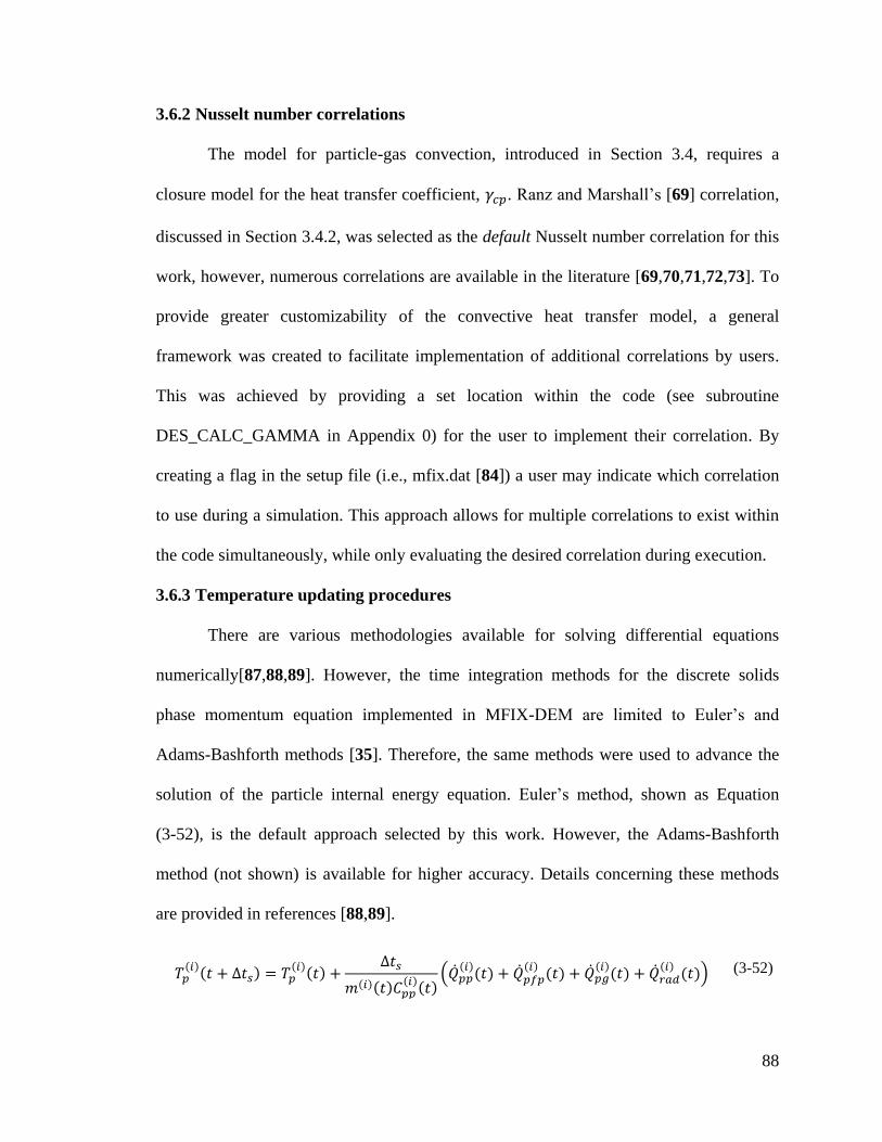
88

3.6.2 Nusselt number correlations

The model for particle-gas convection, introduced in Section 3.4, requires a

closure model for the heat transfer coefficient, . Ranz and Marshall’s [69] correlation,

discussed in Section 3.4.2, was selected as the default Nusselt number correlation for this

work, however, numerous correlations are available in the literature [69,70,71,72,73]. To

provide greater customizability of the convective heat transfer model, a general

framework was created to facilitate implementation of additional correlations by users.

This was achieved by providing a set location within the code (see subroutine

DES_CALC_GAMMA in Appendix 0) for the user to implement their correlation. By

creating a flag in the setup file (i.e., mfix.dat [84]) a user may indicate which correlation

to use during a simulation. This approach allows for multiple correlations to exist within

the code simultaneously, while only evaluating the desired correlation during execution.

3.6.3 Temperature updating procedures

There are various methodologies available for solving differential equations

numerically[87,88,89]. However, the time integration methods for the discrete solids

phase momentum equation implemented in MFIX-DEM are limited to Euler’s and

Adams-Bashforth methods [35]. Therefore, the same methods were used to advance the

solution of the particle internal energy equation. Euler’s method, shown as Equation

(3-52), is the default approach selected by this work. However, the Adams-Bashforth

method (not shown) is available for higher accuracy. Details concerning these methods

are provided in references [88,89].

(3-52)

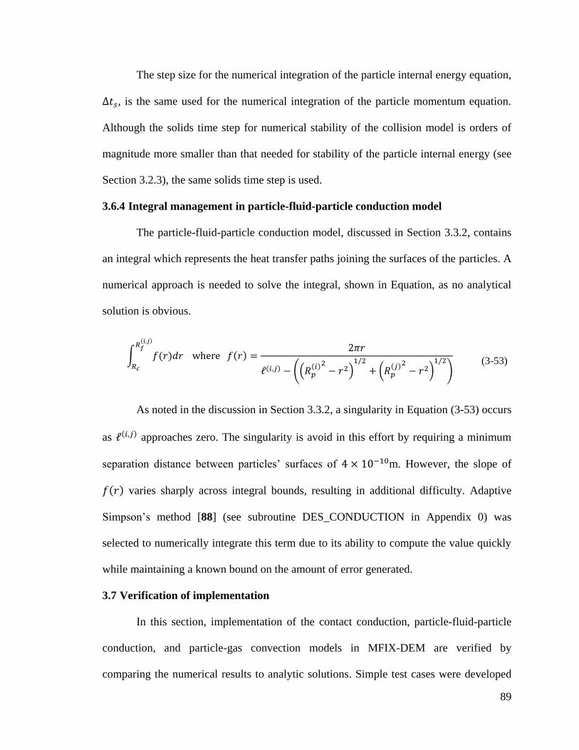
89

The step size for the numerical integration of the particle internal energy equation,

, is the same used for the numerical integration of the particle momentum equation.

Although the solids time step for numerical stability of the collision model is orders of

magnitude more smaller than that needed for stability of the particle internal energy (see

Section 3.2.3), the same solids time step is used.

3.6.4 Integral management in particle-fluid-particle conduction model

The particle-fluid-particle conduction model, discussed in Section 3.3.2, contains

an integral which represents the heat transfer paths joining the surfaces of the particles. A

numerical approach is needed to solve the integral, shown in Equation, as no analytical

solution is obvious.

(3-53)

As noted in the discussion in Section 3.3.2, a singularity in Equation (3-53) occurs

as approaches zero. The singularity is avoid in this effort by requiring a minimum

separation distance between particles’ surfaces of m. However, the slope of

varies sharply across integral bounds, resulting in additional difficulty. Adaptive

Simpson’s method [88] (see subroutine DES_CONDUCTION in Appendix 0) was

selected to numerically integrate this term due to its ability to compute the value quickly

while maintaining a known bound on the amount of error generated.

3.7 Verification of implementation

In this section, implementation of the contact conduction, particle-fluid-particle

conduction, and particle-gas convection models in MFIX-DEM are verified by

comparing the numerical results to analytic solutions. Simple test cases were developed

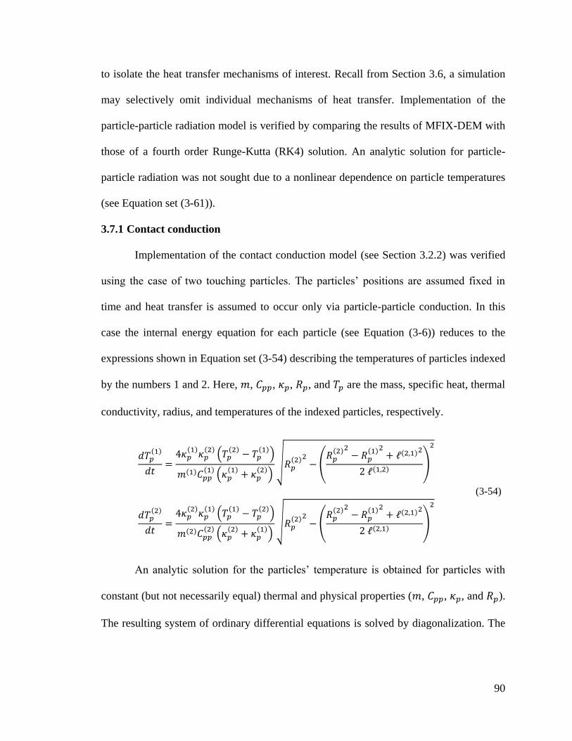
90

to isolate the heat transfer mechanisms of interest. Recall from Section 3.6, a simulation

may selectively omit individual mechanisms of heat transfer. Implementation of the

particle-particle radiation model is verified by comparing the results of MFIX-DEM with

those of a fourth order Runge-Kutta (RK4) solution. An analytic solution for particle-

particle radiation was not sought due to a nonlinear dependence on particle temperatures

(see Equation set (3-61)).

3.7.1 Contact conduction

Implementation of the contact conduction model (see Section 3.2.2) was verified

using the case of two touching particles. The particles’ positions are assumed fixed in

time and heat transfer is assumed to occur only via particle-particle conduction. In this

case the internal energy equation for each particle (see Equation (3-6)) reduces to the

expressions shown in Equation set (3-54) describing the temperatures of particles indexed

by the numbers 1 and 2. Here, , , , , and are the mass, specific heat, thermal

conductivity, radius, and temperatures of the indexed particles, respectively.

(3-54)

An analytic solution for the particles’ temperature is obtained for particles with

constant (but not necessarily equal) thermal and physical properties ( , , , and ).

The resulting system of ordinary differential equations is solved by diagonalization. The

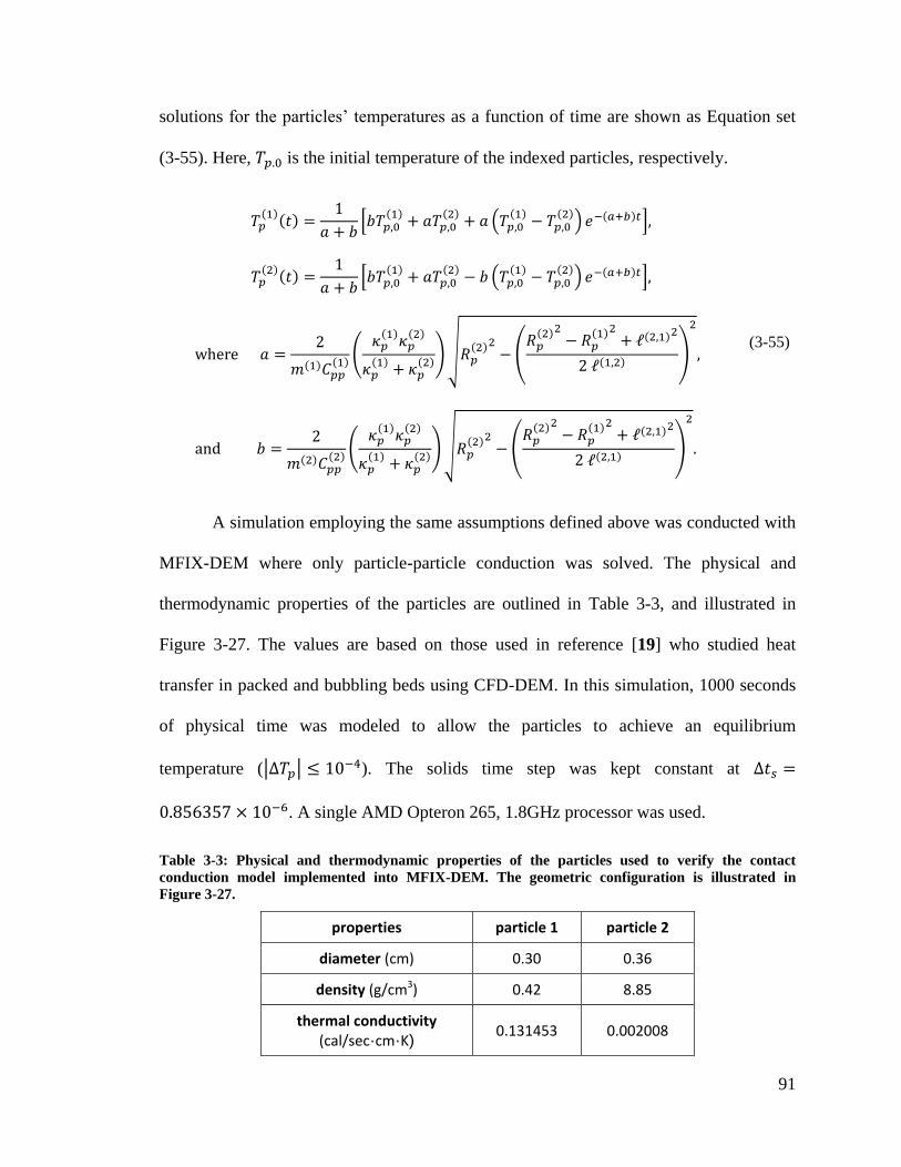
91

solutions for the particles’ temperatures as a function of time are shown as Equation set

(3-55). Here, is the initial temperature of the indexed particles, respectively.

(3-55)

A simulation employing the same assumptions defined above was conducted with

MFIX-DEM where only particle-particle conduction was solved. The physical and

thermodynamic properties of the particles are outlined in Table 3-3, and illustrated in

Figure 3-27. The values are based on those used in reference [19] who studied heat

transfer in packed and bubbling beds using CFD-DEM. In this simulation, 1000 seconds

of physical time was modeled to allow the particles to achieve an equilibrium

temperature ( ). The solids time step was kept constant at

. A single AMD Opteron 265, 1.8GHz processor was used.

Table 3-3: Physical and thermodynamic properties of the particles used to verify the contact

conduction model implemented into MFIX-DEM. The geometric configuration is illustrated in

Figure 3-27.

properties particle 1 particle 2

diameter (cm) 0.30 0.36

density (g/cm3) 0.42 8.85

thermal conductivity (cal/sec·cm·K)

0.131453 0.002008

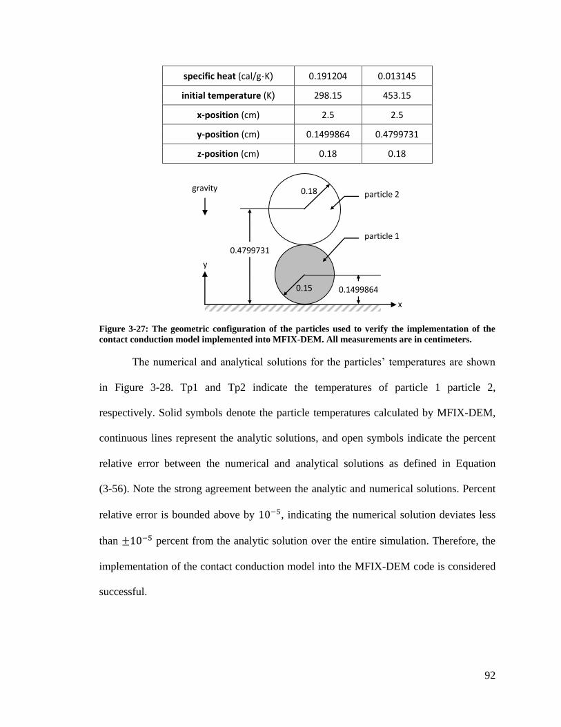
92

specific heat (cal/g·K) 0.191204 0.013145

initial temperature (K) 298.15 453.15

x-position (cm) 2.5 2.5

y-position (cm) 0.1499864 0.4799731

z-position (cm) 0.18 0.18

Figure 3-27: The geometric configuration of the particles used to verify the implementation of the

contact conduction model implemented into MFIX-DEM. All measurements are in centimeters.

The numerical and analytical solutions for the particles’ temperatures are shown

in Figure 3-28. Tp1 and Tp2 indicate the temperatures of particle 1 particle 2,

respectively. Solid symbols denote the particle temperatures calculated by MFIX-DEM,

continuous lines represent the analytic solutions, and open symbols indicate the percent

relative error between the numerical and analytical solutions as defined in Equation

(3-56). Note the strong agreement between the analytic and numerical solutions. Percent

relative error is bounded above by , indicating the numerical solution deviates less

than percent from the analytic solution over the entire simulation. Therefore, the

implementation of the contact conduction model into the MFIX-DEM code is considered

successful.

0.1499864

0.4799731

0.15

0.18 gravity

x

y

particle 2

particle 1

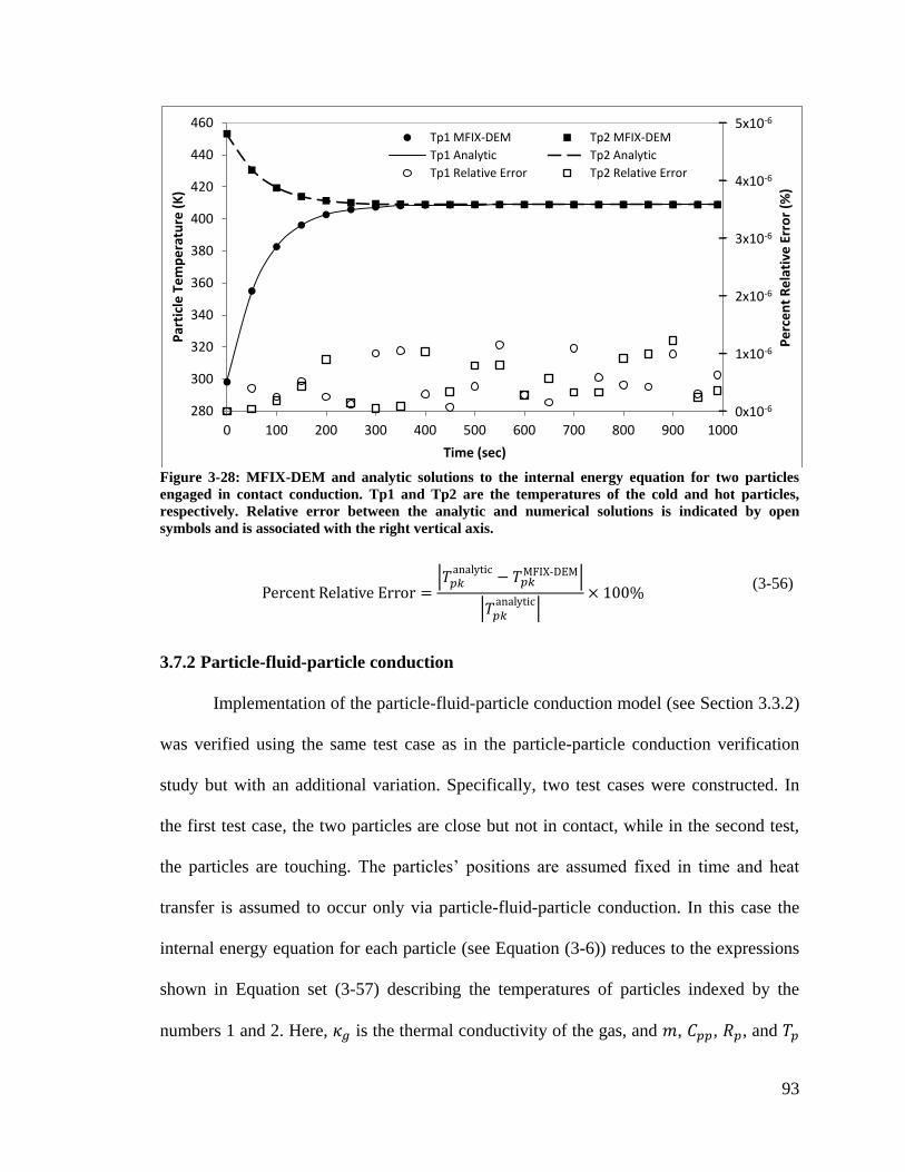
93

Figure 3-28: MFIX-DEM and analytic solutions to the internal energy equation for two particles

engaged in contact conduction. Tp1 and Tp2 are the temperatures of the cold and hot particles,

respectively. Relative error between the analytic and numerical solutions is indicated by open

symbols and is associated with the right vertical axis.

(3-56)

3.7.2 Particle-fluid-particle conduction

Implementation of the particle-fluid-particle conduction model (see Section 3.3.2)

was verified using the same test case as in the particle-particle conduction verification

study but with an additional variation. Specifically, two test cases were constructed. In

the first test case, the two particles are close but not in contact, while in the second test,

the particles are touching. The particles’ positions are assumed fixed in time and heat

transfer is assumed to occur only via particle-fluid-particle conduction. In this case the

internal energy equation for each particle (see Equation (3-6)) reduces to the expressions

shown in Equation set (3-57) describing the temperatures of particles indexed by the

numbers 1 and 2. Here, is the thermal conductivity of the gas, and , , , and

5x10-6

4x10-6

3x10-6

2x10-6

1x10-6

0x10-6 280

300

320

340

360

380

400

420

440

460

0 100 200 300 400 500 600 700 800 900 1000

Pe

rce

nt

Re

lati

ve E

rro

r (%

)

Par

ticl

e T

em

pe

ratu

re (

K)

Time (sec)

Tp1 MFIX-DEM Tp2 MFIX-DEM

Tp1 Analytic Tp2 Analytic

Tp1 Relative Error Tp2 Relative Error

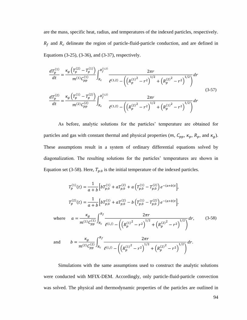
94

are the mass, specific heat, radius, and temperatures of the indexed particles, respectively.

and delineate the region of particle-fluid-particle conduction, and are defined in

Equations (3-25), (3-36), and (3-37), respectively.

(3-57)

As before, analytic solutions for the particles’ temperature are obtained for

particles and gas with constant thermal and physical properties ( , , , , and ).

These assumptions result in a system of ordinary differential equations solved by

diagonalization. The resulting solutions for the particles’ temperatures are shown in

Equation set (3-58). Here, is the initial temperature of the indexed particles.

(3-58)

Simulations with the same assumptions used to construct the analytic solutions

were conducted with MFIX-DEM. Accordingly, only particle-fluid-particle convection

was solved. The physical and thermodynamic properties of the particles are outlined in

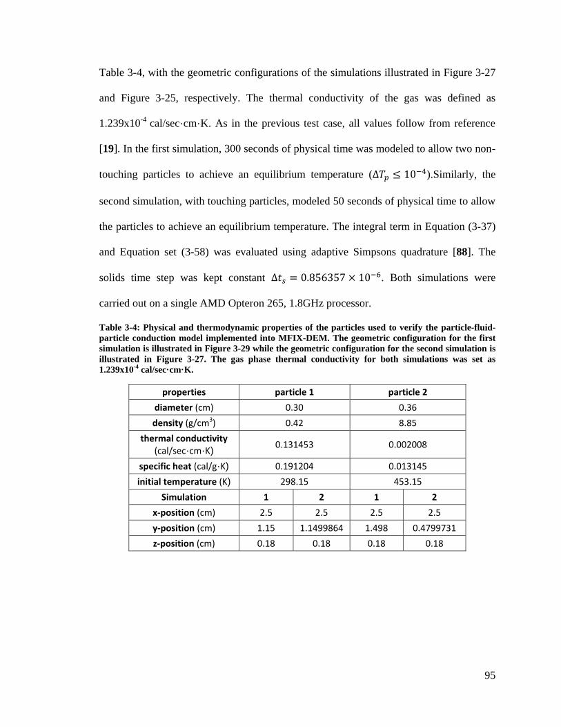
95

Table 3-4, with the geometric configurations of the simulations illustrated in Figure 3-27

and Figure 3-25, respectively. The thermal conductivity of the gas was defined as

1.239x10-4

cal/sec·cm·K. As in the previous test case, all values follow from reference

[19]. In the first simulation, 300 seconds of physical time was modeled to allow two non-

touching particles to achieve an equilibrium temperature ( ).Similarly, the

second simulation, with touching particles, modeled 50 seconds of physical time to allow

the particles to achieve an equilibrium temperature. The integral term in Equation (3-37)

and Equation set (3-58) was evaluated using adaptive Simpsons quadrature [88]. The

solids time step was kept constant . Both simulations were

carried out on a single AMD Opteron 265, 1.8GHz processor.

Table 3-4: Physical and thermodynamic properties of the particles used to verify the particle-fluid-

particle conduction model implemented into MFIX-DEM. The geometric configuration for the first

simulation is illustrated in Figure 3-29 while the geometric configuration for the second simulation is

illustrated in Figure 3-27. The gas phase thermal conductivity for both simulations was set as

1.239x10-4

cal/sec·cm·K.





0.131453 0.002008



Simulation 1 2 1 2

x-position (cm) 2.5 2.5 2.5 2.5

y-position (cm) 1.15 1.1499864 1.498 0.4799731

z-position (cm) 0.18 0.18 0.18 0.18

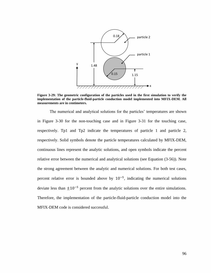
96

Figure 3-29: The geometric configuration of the particles used in the first simulation to verify the

implementation of the particle-fluid-particle conduction model implemented into MFIX-DEM. All

measurements are in centimeters.

The numerical and analytical solutions for the particles’ temperatures are shown

in Figure 3-30 for the non-touching case and in Figure 3-31 for the touching case,

respectively. Tp1 and Tp2 indicate the temperatures of particle 1 and particle 2,


continuous lines represent the analytic solutions, and open symbols indicate the percent

relative error between the numerical and analytical solutions (see Equation (3-56)). Note

the strong agreement between the analytic and numerical solutions. For both test cases,

percent relative error is bounded above by , indicating the numerical solutions

deviate less than percent from the analytic solutions over the entire simulations.

Therefore, the implementation of the particle-fluid-particle conduction model into the

MFIX-DEM code is considered successful.

1.15

1.48

0.15

0.18

x

y

particle 2

particle 1

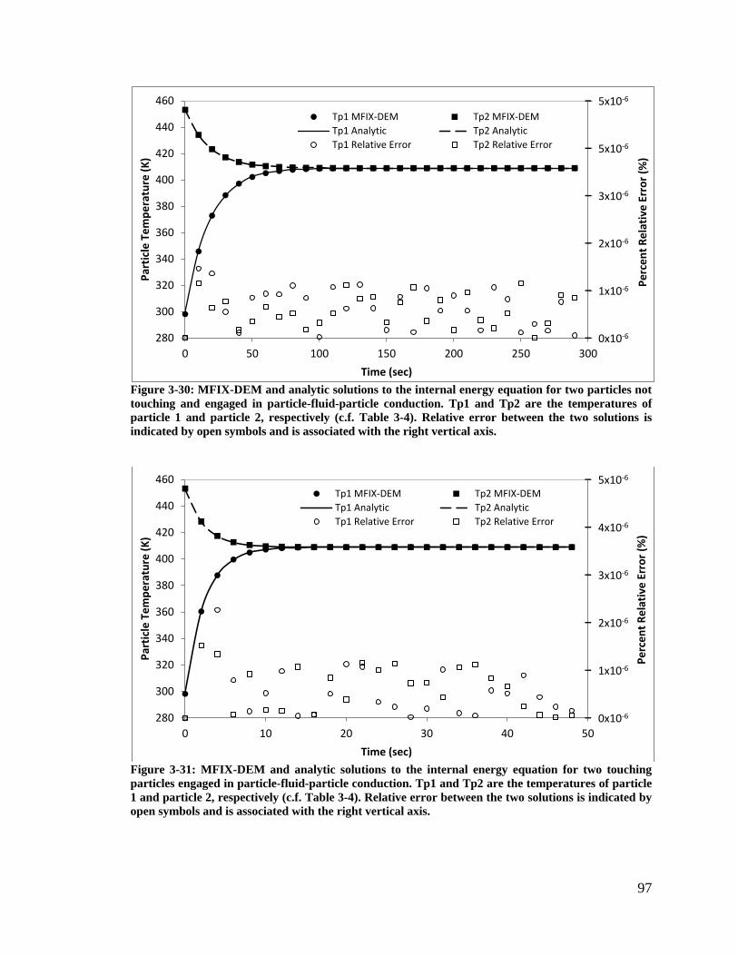
97

Figure 3-30: MFIX-DEM and analytic solutions to the internal energy equation for two particles not

touching and engaged in particle-fluid-particle conduction. Tp1 and Tp2 are the temperatures of

particle 1 and particle 2, respectively (c.f. Table 3-4). Relative error between the two solutions is

indicated by open symbols and is associated with the right vertical axis.

Figure 3-31: MFIX-DEM and analytic solutions to the internal energy equation for two touching

particles engaged in particle-fluid-particle conduction. Tp1 and Tp2 are the temperatures of particle

1 and particle 2, respectively (c.f. Table 3-4). Relative error between the two solutions is indicated by

open symbols and is associated with the right vertical axis.

5x10-6

5x10-6

3x10-6

2x10-6

1x10-6

0x10-6 280

300

320

340

360

380

400

420

440

460

0 50 100 150 200 250 300

Pe

rce

nt

Re

lati

ve E

rro

r (%

)

Par

ticl

e T

em

pe

ratu

re (

K)

Time (sec)




5x10-6

4x10-6

3x10-6

2x10-6

1x10-6

0x10-6 280

300

320

340

360

380

400

420

440

460

0 10 20 30 40 50

Pe

rce

nt

Re

lati

ve E

rro

r (%

)

Par

ticl

e T

em

pe

ratu

re (

K)

Time (sec)




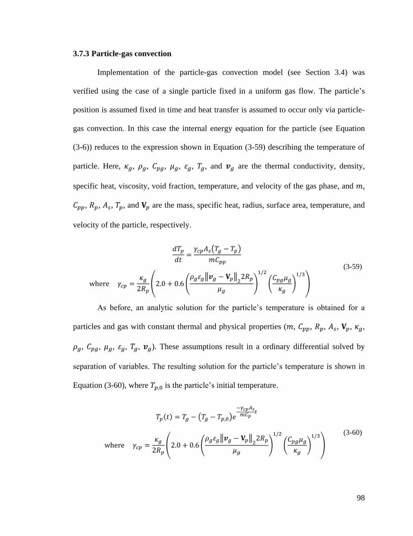
98

3.7.3 Particle-gas convection

Implementation of the particle-gas convection model (see Section 3.4) was

verified using the case of a single particle fixed in a uniform gas flow. The particle’s

position is assumed fixed in time and heat transfer is assumed to occur only via particle-

gas convection. In this case the internal energy equation for the particle (see Equation

(3-6)) reduces to the expression shown in Equation (3-59) describing the temperature of

particle. Here, , , , , , , and are the thermal conductivity, density,

specific heat, viscosity, void fraction, temperature, and velocity of the gas phase, and ,

, , , , and are the mass, specific heat, radius, surface area, temperature, and

velocity of the particle, respectively.

(3-59)

As before, an analytic solution for the particle’s temperature is obtained for a

particles and gas with constant thermal and physical properties ( , , , , , ,

, , , , , ). These assumptions result in a ordinary differential solved by

separation of variables. The resulting solution for the particle’s temperature is shown in

Equation (3-60), where is the particle’s initial temperature.

(3-60)

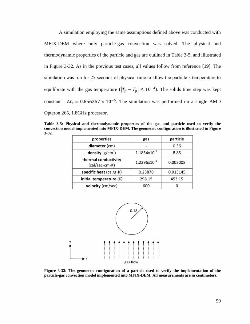
99


MFIX-DEM where only particle-gas convection was solved. The physical and

thermodynamic properties of the particle and gas are outlined in Table 3-5, and illustrated

in Figure 3-32. As in the previous test cases, all values follow from reference [19]. The

simulation was run for 25 seconds of physical time to allow the particle’s temperature to

equilibrate with the gas temperature ( ). The solids time step was kept

constant . The simulation was performed on a single AMD

Opteron 265, 1.8GHz processor.

Table 3-5: Physical and thermodynamic properties of the gas and particle used to verify the

convection model implemented into MFIX-DEM. The geometric configuration is illustrated in Figure

3-32.

properties gas particle

diameter (cm) - 0.36

density (g/cm3) 1.1854x10-3 8.85


1.2396x10-4 0.002008



velocity (cm/sec) 600 0

Figure 3-32: The geometric configuration of a particle used to verify the implementation of the

particle-gas convection model implemented into MFIX-DEM. All measurements are in centimeters.

0.18

x

y

gas flow

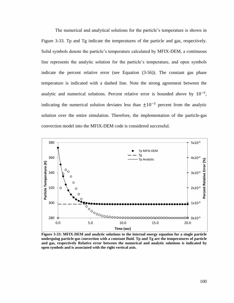
100

The numerical and analytical solutions for the particle’s temperature is shown in

Figure 3-33. Tp and Tg indicate the temperatures of the particle and gas, respectively.

Solid symbols denote the particle’s temperature calculated by MFIX-DEM, a continuous

line represents the analytic solution for the particle’s temperature, and open symbols

indicate the percent relative error (see Equation (3-56)). The constant gas phase

temperature is indicated with a dashed line. Note the strong agreement between the

analytic and numerical solutions. Percent relative error is bounded above by ,

indicating the numerical solution deviates less than percent from the analytic

solution over the entire simulation. Therefore, the implementation of the particle-gas

convection model into the MFIX-DEM code is considered successful.

Figure 3-33: MFIX-DEM and analytic solutions to the internal energy equation for a single particle

undergoing particle-gas convection with a constant fluid. Tp and Tg are the temperatures of particle

and gas, respectively Relative error between the numerical and analytic solutions is indicated by

open symbols and is associated with the right vertical axis.

5x10-6

4x10-6

3x10-6

2x10-6

1x10-6

0x10-6 280

300

320

340

360

380

0.0 5.0 10.0 15.0 20.0

Pe

rce

nt

Re

lati

ve E

rro

r (%

)

Par

ticl

e T

em

pe

ratu

re (

K)

Time (sec)

Tp MFIX-DEM Tg Tp Analytic

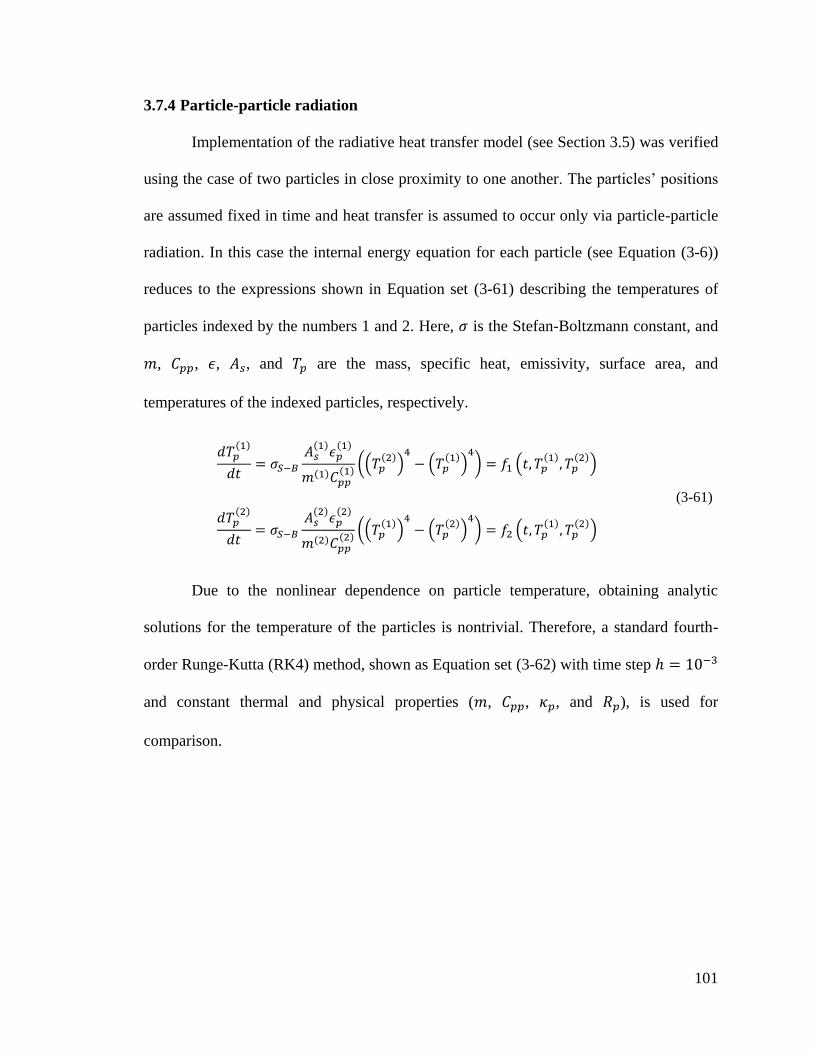
101

3.7.4 Particle-particle radiation

Implementation of the radiative heat transfer model (see Section 3.5) was verified

using the case of two particles in close proximity to one another. The particles’ positions

are assumed fixed in time and heat transfer is assumed to occur only via particle-particle

radiation. In this case the internal energy equation for each particle (see Equation (3-6))

reduces to the expressions shown in Equation set (3-61) describing the temperatures of

particles indexed by the numbers 1 and 2. Here, is the Stefan-Boltzmann constant, and

, , , , and are the mass, specific heat, emissivity, surface area, and

temperatures of the indexed particles, respectively.

(3-61)

Due to the nonlinear dependence on particle temperature, obtaining analytic

solutions for the temperature of the particles is nontrivial. Therefore, a standard fourth-

order Runge-Kutta (RK4) method, shown as Equation set (3-62) with time step

and constant thermal and physical properties ( , , , and ), is used for

comparison.

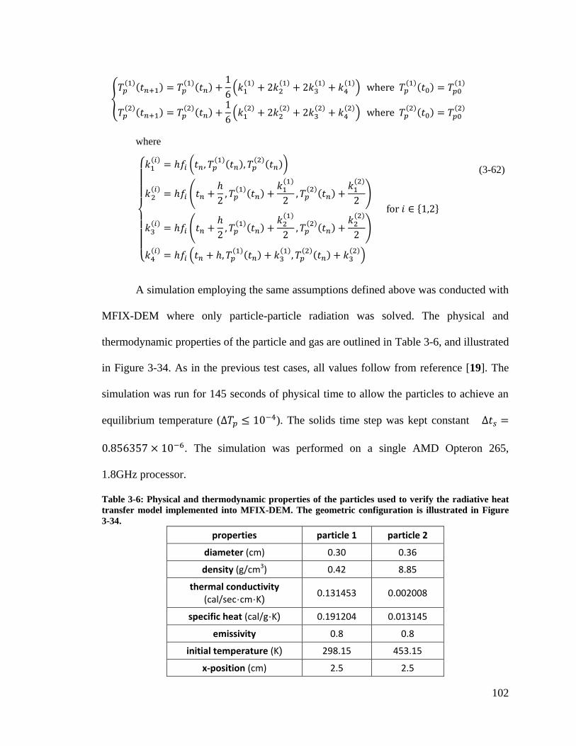
102

where

(3-62)


MFIX-DEM where only particle-particle radiation was solved. The physical and

thermodynamic properties of the particle and gas are outlined in Table 3-6, and illustrated

in Figure 3-34. As in the previous test cases, all values follow from reference [19]. The

simulation was run for 145 seconds of physical time to allow the particles to achieve an

equilibrium temperature ( ). The solids time step was kept constant

. The simulation was performed on a single AMD Opteron 265,

1.8GHz processor.

Table 3-6: Physical and thermodynamic properties of the particles used to verify the radiative heat

transfer model implemented into MFIX-DEM. The geometric configuration is illustrated in Figure

3-34.





0.131453 0.002008


emissivity 0.8 0.8


x-position (cm) 2.5 2.5

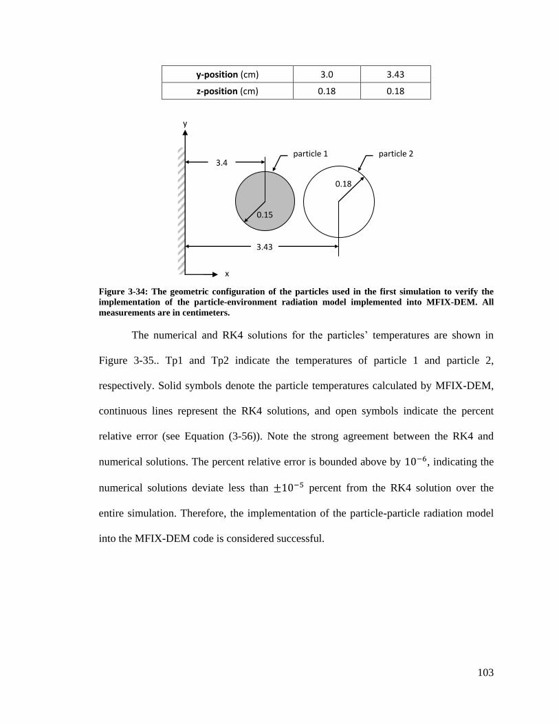
103

y-position (cm) 3.0 3.43

z-position (cm) 0.18 0.18

Figure 3-34: The geometric configuration of the particles used in the first simulation to verify the

implementation of the particle-environment radiation model implemented into MFIX-DEM. All

measurements are in centimeters.

The numerical and RK4 solutions for the particles’ temperatures are shown in

Figure 3-35.. Tp1 and Tp2 indicate the temperatures of particle 1 and particle 2,


continuous lines represent the RK4 solutions, and open symbols indicate the percent

relative error (see Equation (3-56)). Note the strong agreement between the RK4 and

numerical solutions. The percent relative error is bounded above by , indicating the

numerical solutions deviate less than percent from the RK4 solution over the

entire simulation. Therefore, the implementation of the particle-particle radiation model

into the MFIX-DEM code is considered successful.

0.15

0.18

x

y

particle 1 particle 2

3.43

3.4

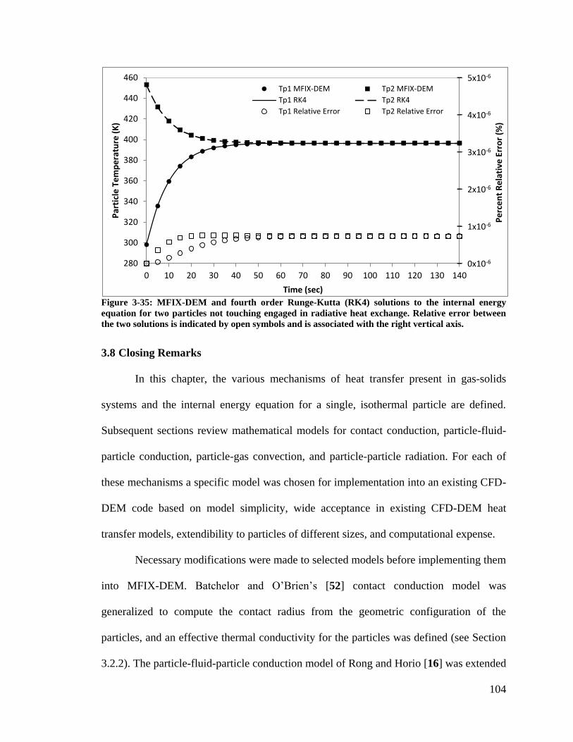
104

Figure 3-35: MFIX-DEM and fourth order Runge-Kutta (RK4) solutions to the internal energy

equation for two particles not touching engaged in radiative heat exchange. Relative error between

the two solutions is indicated by open symbols and is associated with the right vertical axis.

3.8 Closing Remarks

In this chapter, the various mechanisms of heat transfer present in gas-solids

systems and the internal energy equation for a single, isothermal particle are defined.

Subsequent sections review mathematical models for contact conduction, particle-fluid-

particle conduction, particle-gas convection, and particle-particle radiation. For each of

these mechanisms a specific model was chosen for implementation into an existing CFD-

DEM code based on model simplicity, wide acceptance in existing CFD-DEM heat

transfer models, extendibility to particles of different sizes, and computational expense.

Necessary modifications were made to selected models before implementing them

into MFIX-DEM. Batchelor and O’Brien’s [52] contact conduction model was

generalized to compute the contact radius from the geometric configuration of the

particles, and an effective thermal conductivity for the particles was defined (see Section

3.2.2). The particle-fluid-particle conduction model of Rong and Horio [16] was extended

5x10-6

4x10-6

3x10-6

2x10-6

1x10-6

0x10-6 280

300

320

340

360

380

400

420

440

460

0 10 20 30 40 50 60 70 80 90 100 110 120 130 140

Pe

rce

nt

Re

lati

ve E

rro

r (%

)

Par

ticl

e T

em

pe

ratu

re (

K)

Time (sec)


Tp1 RK4 Tp2 RK4


105

to account for particles of different sizes (see Section 3.3.2). For particle-particle

radiation, a new environment temperature was established (see Section 3.5.2).

Finally, the implementation of each model was verified for simple two particle

test cases, or in the case of gas-particle convection, a single fixed particle in a flowing

gas. Strong agreement was observed between the simulation data and the analytic or

numerical solution.

106

Chapter 4: Particle-gas reactive chemistry interface

Chemical reactions in gas-solids flows may occur within a single phase

(homogeneous) or they may require the presence of at least two phases (heterogeneous)

[90]. Presently, MFIX, the CFD code portion of the CFD-DEM model employed in this

work (MFIX-DEM), is capable of modeling user-defined homogeneous and

heterogeneous chemical reactions among continuum phases (i.e., Eulerian-Eulerian

models only) [91,92]. The goal of this effort is to develop and implement a mathematical

interface for managing user-defined heterogeneous chemical reactions among the gas and

discrete solids phases in MFIX-DEM.

This chapter begins by briefly defining the (1) reaction rate, (2) specific heat, (3)

heat of reaction, and (4) individual particle mass and species equations in Section 4.1.

Three particle reaction models and their employment in existing CFD-DEM reactive

chemistry models are presented in Section 4.2. Finally, the algorithmic implementation

and verification of the mathematical interface for managing user-defined particle-gas

chemical reactions developed in this effort are given in Sections 4.3 and 4.4.

4.1 Foundations for particle-gas reactive chemistry

In this section, specific concepts of reactive chemistry referenced in this work are

introduced. This is done to provide a foundation for the topics managed by the

mathematical interface for user-defined chemical reactions. Additional details concerning

the fundamentals of reactive chemistry are found in references [28,90,93,94].

107

4.1.1 Reaction rate

Various interrelated definitions for the rate at which a chemical reaction

progresses, termed the rate of reaction, are available [90]. Therefore, care is needed to

avoid ambiguity. This work defines the rate of reaction with respect to species as the

number of moles of species formed (or consumed) per unit time, per unit surface area

of a particle (e.g., mol·cm-2·s-1

). Specifically, if species is a reactant, then the rate of

reaction is termed the rate of disappearance of species and is notated as . Likewise,

if species A is a product of the reaction, then the reaction rate is termed the rate of

formation of species and notated as . The rate of disappearance is assigned a negative

sign because the reaction rate is always specified as a non-negative number [93].

Defining the rate of reaction with respect to particle surface area is natural in the

context of CFD-DEM as it allows for a 'per particle' treatment of particle-gas reactions.

Other definitions (e.g., per volume of fluid or per reactor volume) may require averaging

rates of formation and rates of disappearance of the solids phase species from a collection

of particles contained within some control volume. This may, in effect, remove the

distinct advantage of CFD-DEM modeling (i.e., the ability to track the conversion of

individual particles during a chemical reaction).

The rate equation for a reaction (also referred to as a rate law) is an algebraic

function which gives the reaction rate in terms of material properties [95]. An example

rate law for the rate of formation of species is shown in Equation (4-1). Here, is the

rate coefficient (also called the rate constant), and are the concentration of

reactants and , and and are empirically fitted constants.

108

(4-1)

Once the rate of reaction with respect to a particular species is specified, the rates

of formation and disappearance of the other reactants and products are obtained from the

reaction stoichiometry. For example, consider the generic reaction shown in Equation

(4-2). Here, molecules of species and molecules of species are destroyed to

produce molecules of species and molecules of species . The terms in parentheses

indicate whether the species belongs to the gas or solids phase. The proportional

relationship linking the rates of disappearance of species and and the rates of

formation of species and are given in Equation (4-3).

(4-2)

(4-3)

Reactions where the reactants are consumed to form products, but the products do

not react to form the reactants are termed irreversible and require a single reaction rate.

The example reaction shown in Equation (4-2) is irreversible as indicated by the symbol

( ). However, rate equations are needed for both the forward and backward directions in

reversible reactions, commonly indicated by the symbol ( ). If the example reaction in

Equation (4-2) were reversible, a reaction rate for the backward direction, potentially a

function of the concentrations of species and , is needed.

4.1.2 Specific Heat

The amount of heat required to increase a material’s temperature one degree,

while holding the pressure or volume constant is termed the heat capacity [96]. The heat

capacity at constant pressure is notated as , and the heat capacity at constant volume is

109

notated .The term specific heat is used to denote a heat capacity defined on a per unit

mass basis. The specific heat of a material is a function of its temperature and commonly

given as a polynomial [97]. Details concerning the calculation of specific heats in this

effort are reserved for Section 4.3.3.

4.1.3 Heat of reaction

The amount of heat liberated or absorbed during a reaction, termed the heat of

reaction ( ), is given by the difference in enthalpies between the products and reactants

[90]. The change in enthalpy for endothermic reactions is positive, indicating that energy

from the system is needed to facilitate the reaction. Conversely, the change in enthalpy

for exothermic reactions is negative, signifying that energy is released to the system

during the reaction. The heat of reaction for the generic reaction given by Equation (4-2)

is illustrated by Equation (4-4). Here, and are the enthalpies of the products, and

and are the enthalpies of the reactants.

(4-4)

The enthalpy for species at temperature ( ) is given by Equation (4-5).

Here, is species ’s enthalpy of formation at reference temperature , and

is the enthalpy change caused by a change in temperature (i.e., from to )

[93]. The species change in enthalpy ( ) is calculated by integrating the material’s

specific heat ( ) with respect to temperature, as shown by Equation (4-6). Details

concerning the calculation of enthalpies in this effort are reserved for Section 4.3.4.

(4-5)

110

(4-6)

In reactions where mass is transferred from one phase to another (e.g., solids and

gas phase species react to produce a different gas phase species), accounting for the

transfer of enthalpy with the transferred mass is needed. Consider the example reaction

shown in Equation (4-2). Suppose that there is a net production of gas phase species

and, in turn, a net consumption of solids phase species (i.e., there is a net transfer of

mass from the solids phase to the gas phase). The rate of enthalpy transfer as a result of

mass transfer is then given by Equation (4-7). As before, – and are the rate of

disappearance and formation of solids species and , and is the enthalpy of species

at the local gas phase conditions. If there are multiple destination phase products, care

is needed to ensure that the rate of enthalpy transfer ( ) is computed from the correct

proportions and enthalpies of the various species generated.

(4-7)

The usage of the transferred species’ enthalpy at the destination phase’s

conditions is attributed to the wet bulb effect [98]. For example, as air passes over a wet

wick covering a thermometer’s bulb, some of the water evaporates. This causes the

water’s temperature to drop (i.e., the temperature reading on the thermometer drops).

Once the temperature of the water stabilizes (i.e., there is a constant temperature reading

from the thermometer), the heat loss from the water due to evaporation equals the heat

gained by the water from the air. Otherwise, if energy from air was not transferred to the

water, the water’s temperature would continue to drop [99].

111

The heat of reaction and enthalpy transfer due to mass transfer are combined into

source terms for the gas and particle internal energy equations ( in Equation (1-6)

and in Equation (3-6)). Since the heat of reaction is calculated for a reaction in

general, a methodology for distributing the energy among the gas and solids phases is

needed. The approach for assigning the heat of reaction employed in this effort is

reserved for Section 4.3.5.

4.1.4 Mass and species equations for a particle

The time rate of change of a particle’s mass resulting from a chemical reaction or

phase change is given by Equation (4-8). Here,

is the mass of the indexed particle,

and

is the rate of production (or consumption) of species for the indexed particle.

The superscript over the summation,

, is the total number of species that comprise

particle . The sign convention is such that is positive if species is produced and

negative when consumed. Furthermore, is obtained from expressions like Equations

(4-1) and (4-3) and specific to the reaction of interest.

(4-8)

The time rate of change of the species’ mass in particle is given by

Equation (4-9). Here,

is species ’s mass fraction of the indexed particle. For a

particle comprised by

species,

equations of this form are needed to account for

the composition of the particle. Employing the product rule and combing the result with

Equation (4-8) yields an equation for the species mass fraction, shown as (4-10).

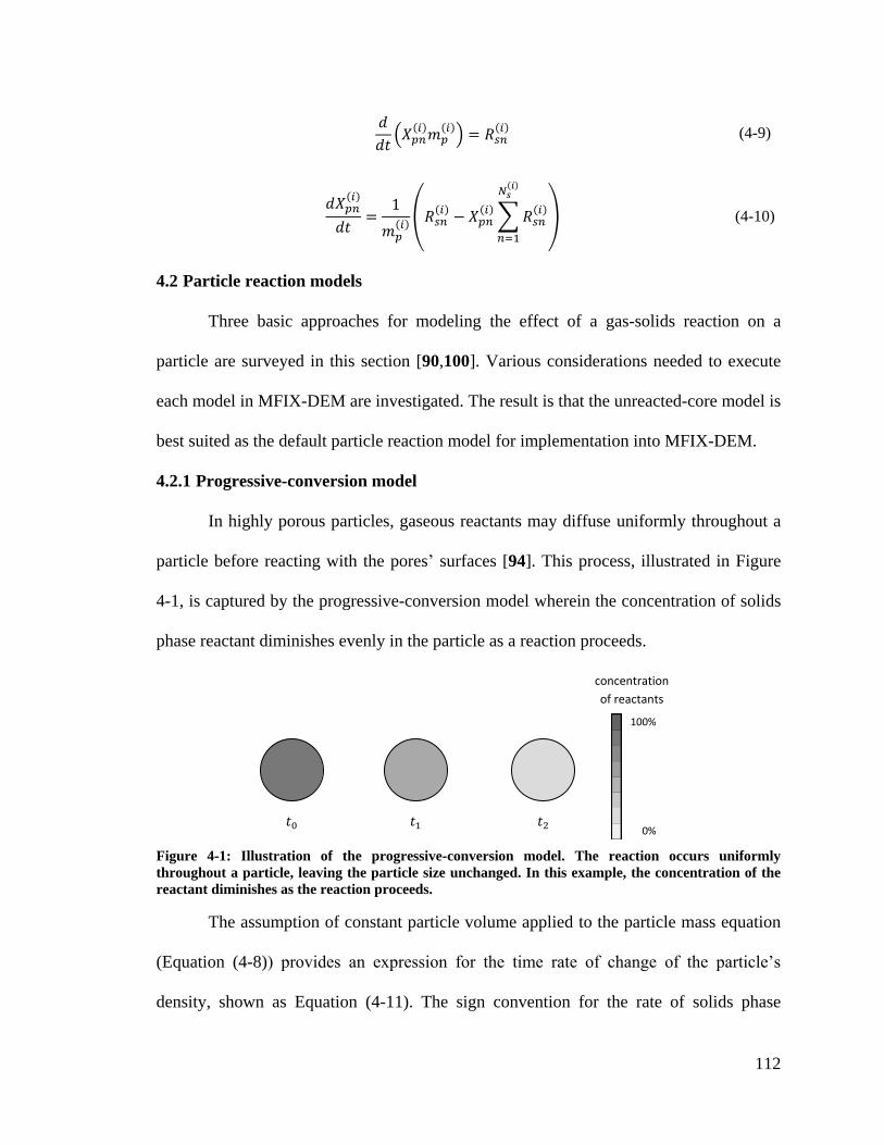
112

(4-9)

(4-10)

4.2 Particle reaction models

Three basic approaches for modeling the effect of a gas-solids reaction on a

particle are surveyed in this section [90,100]. Various considerations needed to execute

each model in MFIX-DEM are investigated. The result is that the unreacted-core model is

best suited as the default particle reaction model for implementation into MFIX-DEM.

4.2.1 Progressive-conversion model

In highly porous particles, gaseous reactants may diffuse uniformly throughout a

particle before reacting with the pores’ surfaces [94]. This process, illustrated in Figure

4-1, is captured by the progressive-conversion model wherein the concentration of solids

phase reactant diminishes evenly in the particle as a reaction proceeds.

Figure 4-1: Illustration of the progressive-conversion model. The reaction occurs uniformly

throughout a particle, leaving the particle size unchanged. In this example, the concentration of the

reactant diminishes as the reaction proceeds.

The assumption of constant particle volume applied to the particle mass equation

(Equation (4-8)) provides an expression for the time rate of change of the particle’s

density, shown as Equation (4-11). The sign convention for the rate of solids phase

concentration

of reactants

100%

0%

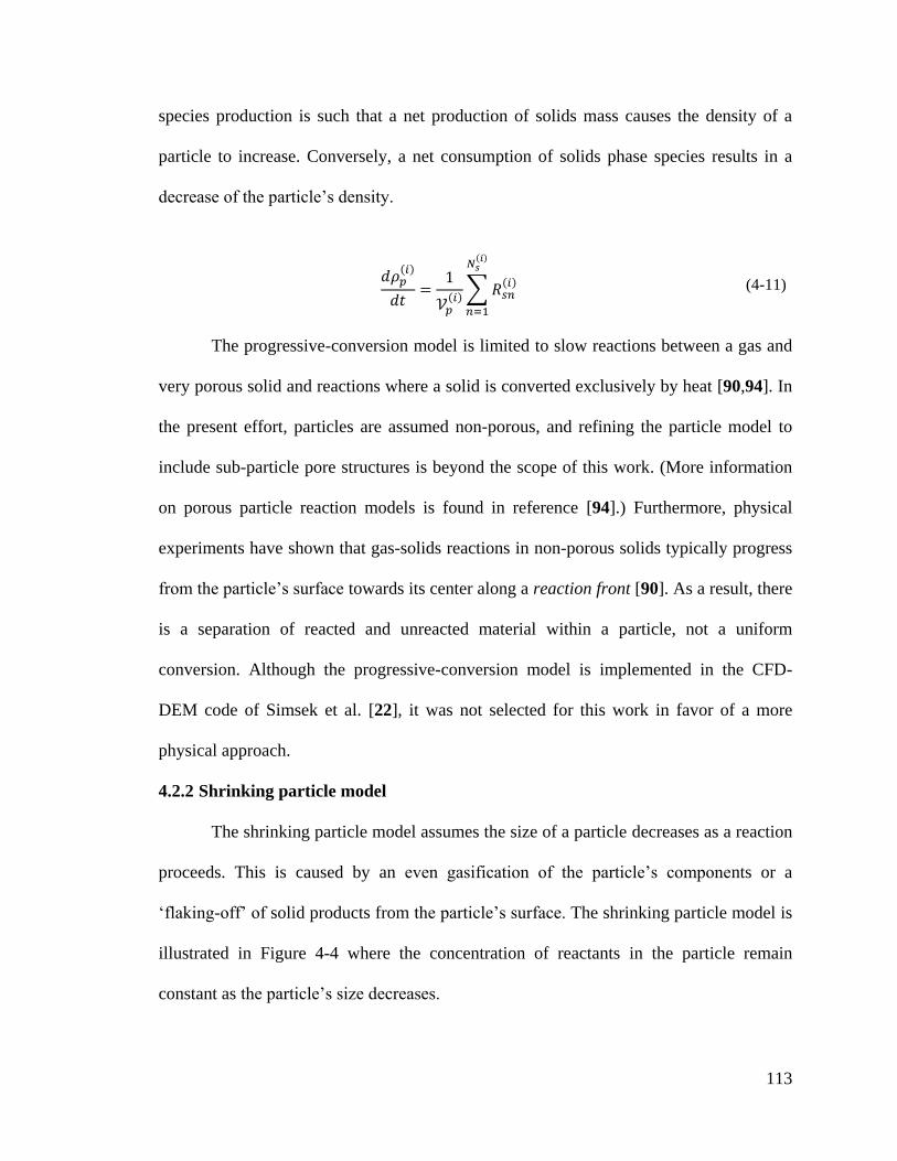
113

species production is such that a net production of solids mass causes the density of a

particle to increase. Conversely, a net consumption of solids phase species results in a

decrease of the particle’s density.

(4-11)

The progressive-conversion model is limited to slow reactions between a gas and

very porous solid and reactions where a solid is converted exclusively by heat [90,94]. In

the present effort, particles are assumed non-porous, and refining the particle model to

include sub-particle pore structures is beyond the scope of this work. (More information

on porous particle reaction models is found in reference [94].) Furthermore, physical

experiments have shown that gas-solids reactions in non-porous solids typically progress

from the particle’s surface towards its center along a reaction front [90]. As a result, there

is a separation of reacted and unreacted material within a particle, not a uniform

conversion. Although the progressive-conversion model is implemented in the CFD-

DEM code of Simsek et al. [22], it was not selected for this work in favor of a more

physical approach.

4.2.2 Shrinking particle model

The shrinking particle model assumes the size of a particle decreases as a reaction

proceeds. This is caused by an even gasification of the particle’s components or a

‘flaking-off’ of solid products from the particle’s surface. The shrinking particle model is

illustrated in Figure 4-4 where the concentration of reactants in the particle remain

constant as the particle’s size decreases.

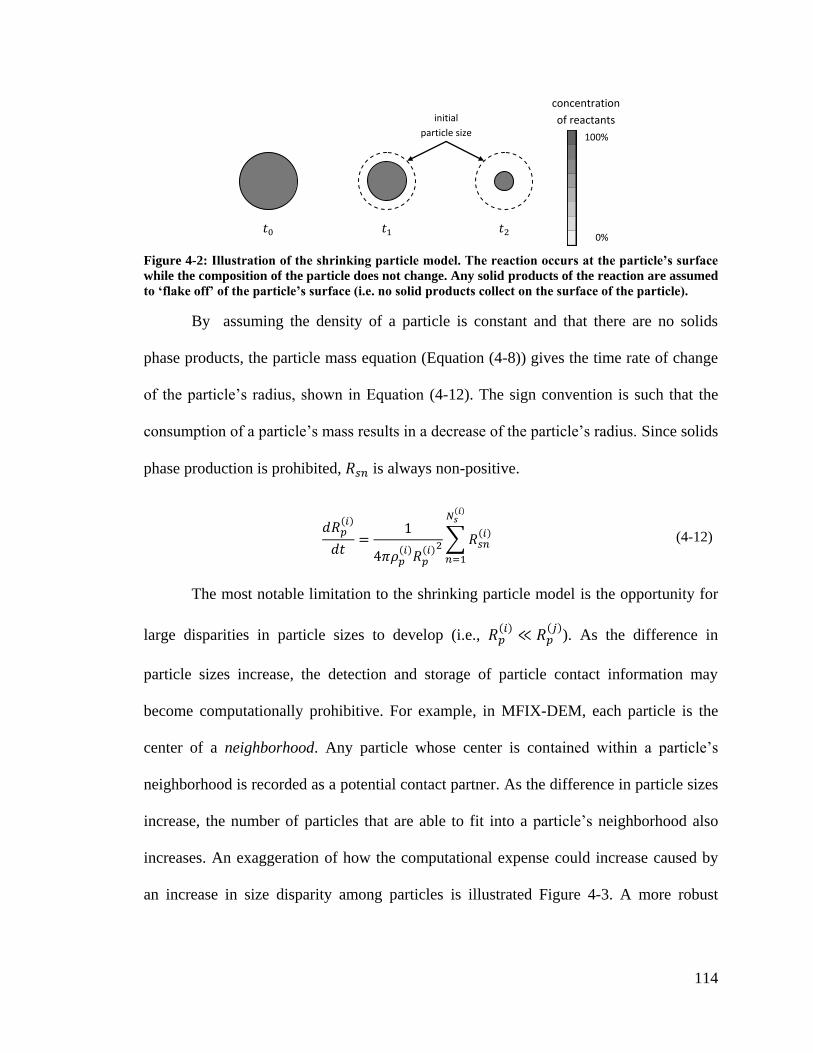
114

Figure 4-2: Illustration of the shrinking particle model. The reaction occurs at the particle’s surface

while the composition of the particle does not change. Any solid products of the reaction are assumed

to ‘flake off’ of the particle’s surface (i.e. no solid products collect on the surface of the particle).

By assuming the density of a particle is constant and that there are no solids

phase products, the particle mass equation (Equation (4-8)) gives the time rate of change

of the particle’s radius, shown in Equation (4-12). The sign convention is such that the

consumption of a particle’s mass results in a decrease of the particle’s radius. Since solids

phase production is prohibited, is always non-positive.

(4-12)

The most notable limitation to the shrinking particle model is the opportunity for

large disparities in particle sizes to develop (i.e.,

). As the difference in

particle sizes increase, the detection and storage of particle contact information may

become computationally prohibitive. For example, in MFIX-DEM, each particle is the

center of a neighborhood. Any particle whose center is contained within a particle’s

neighborhood is recorded as a potential contact partner. As the difference in particle sizes

increase, the number of particles that are able to fit into a particle’s neighborhood also

increases. An exaggeration of how the computational expense could increase caused by

an increase in size disparity among particles is illustrated Figure 4-3. A more robust

concentration

of reactants

100%

0%

initial

particle size

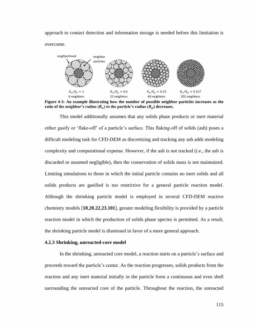
115

approach to contact detection and information storage is needed before this limitation is

overcome.

Figure 4-3: An example illustrating how the number of possible neighbor particles increases as the

ratio of the neighbor’s radius ( ) to the particle’s radius ( ) decreases.

This model additionally assumes that any solids phase products or inert material

either gasify or ‘flake-off’ of a particle’s surface. This flaking-off of solids (ash) poses a

difficult modeling task for CFD-DEM as discretizing and tracking any ash adds modeling

complexity and computational expense. However, if the ash is not tracked (i.e., the ash is

discarded or assumed negligible), then the conservation of solids mass is not maintained.

Limiting simulations to those in which the initial particle contains no inert solids and all

solids products are gasified is too restrictive for a general particle reaction model.

Although the shrinking particle model is employed in several CFD-DEM reactive

chemistry models [18,20,22,23,101], greater modeling flexibility is provided by a particle

reaction model in which the production of solids phase species is permitted. As a result,

the shrinking particle model is dismissed in favor of a more general approach.

4.2.3 Shrinking, unreacted-core model

In the shrinking, unreacted core model, a reaction starts on a particle’s surface and

proceeds toward the particle’s center. As the reaction progresses, solids products from the

reaction and any inert material initially in the particle form a continuous and even shell

surrounding the unreacted core of the particle. Throughout the reaction, the unreacted

22 neighbors

202 neighbors

6 neighbors

neighbor

particles

60 neighbors

neighborhood

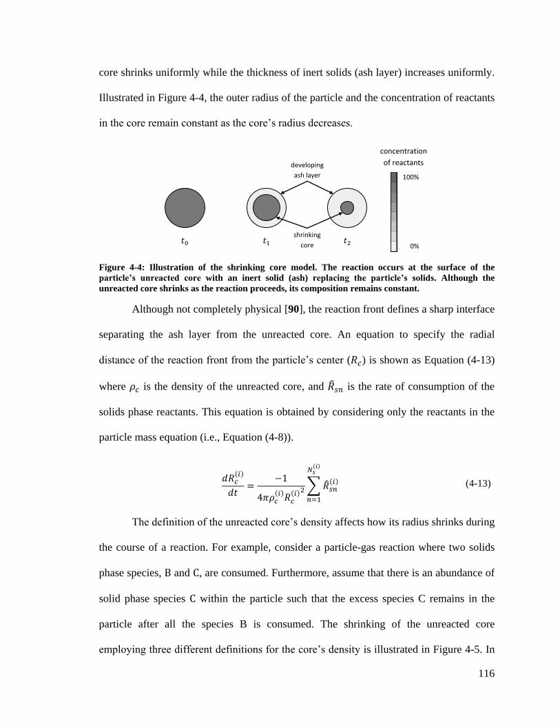
116

core shrinks uniformly while the thickness of inert solids (ash layer) increases uniformly.

Illustrated in Figure 4-4, the outer radius of the particle and the concentration of reactants

in the core remain constant as the core’s radius decreases.

Figure 4-4: Illustration of the shrinking core model. The reaction occurs at the surface of the

particle’s unreacted core with an inert solid (ash) replacing the particle’s solids. Although the

unreacted core shrinks as the reaction proceeds, its composition remains constant.

Although not completely physical [90], the reaction front defines a sharp interface

separating the ash layer from the unreacted core. An equation to specify the radial

distance of the reaction front from the particle’s center ( ) is shown as Equation (4-13)

where is the density of the unreacted core, and is the rate of consumption of the

solids phase reactants. This equation is obtained by considering only the reactants in the

particle mass equation (i.e., Equation (4-8)).

(4-13)

The definition of the unreacted core’s density affects how its radius shrinks during

the course of a reaction. For example, consider a particle-gas reaction where two solids

phase species, and , are consumed. Furthermore, assume that there is an abundance of

solid phase species within the particle such that the excess species C remains in the

particle after all the species B is consumed. The shrinking of the unreacted core

employing three different definitions for the core’s density is illustrated in Figure 4-5. In

developing

ash layer

shrinking

core

concentration

of reactants

100%

0%

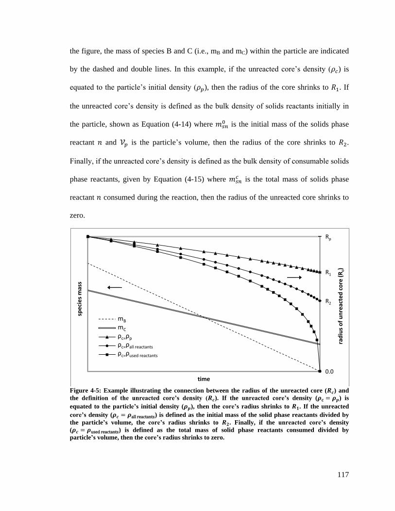
117

the figure, the mass of species B and C (i.e., mB and mC) within the particle are indicated

by the dashed and double lines. In this example, if the unreacted core’s density ( ) is

equated to the particle’s initial density ( ), then the radius of the core shrinks to . If

the unreacted core’s density is defined as the bulk density of solids reactants initially in

the particle, shown as Equation (4-14) where is the initial mass of the solids phase

reactant and is the particle’s volume, then the radius of the core shrinks to .

Finally, if the unreacted core’s density is defined as the bulk density of consumable solids

phase reactants, given by Equation (4-15) where is the total mass of solids phase

reactant consumed during the reaction, then the radius of the unreacted core shrinks to

zero.

Figure 4-5: Example illustrating the connection between the radius of the unreacted core ( ) and

the definition of the unreacted core’s density ( ). If the unreacted core’s density ( ) is

equated to the particle’s initial density ( ), then the core’s radius shrinks to . If the unreacted

core’s density ( ) is defined as the initial mass of the solid phase reactants divided by

the particle’s volume, the core’s radius shrinks to . Finally, if the unreacted core’s density

( ) is defined as the total mass of solid phase reactants consumed divided by

particle’s volume, then the core’s radius shrinks to zero.

Rp

R1

R2

0.0

rad

ius

of

un

reac

ted

co

re (

Rc)

spe

cie

s m

ass

time

mB mC

ρc=ρp

ρc=ρall reactants

ρc=ρused reactants

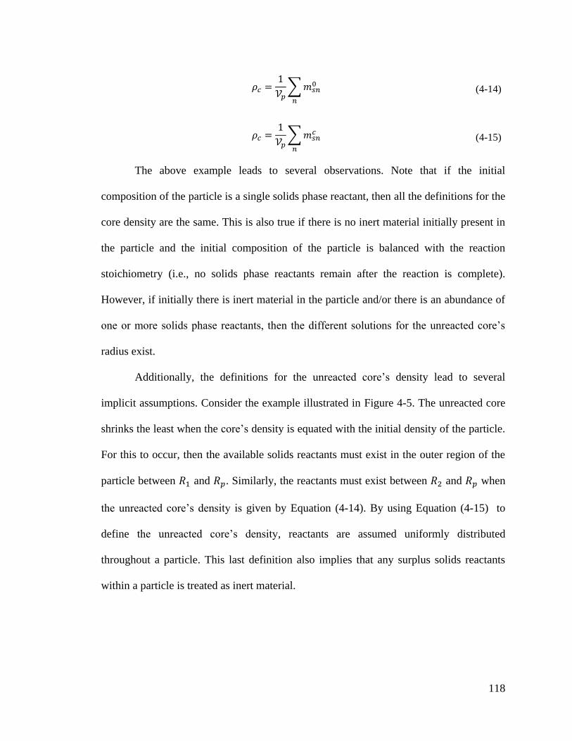
118

(4-14)

(4-15)

The above example leads to several observations. Note that if the initial

composition of the particle is a single solids phase reactant, then all the definitions for the

core density are the same. This is also true if there is no inert material initially present in

the particle and the initial composition of the particle is balanced with the reaction

stoichiometry (i.e., no solids phase reactants remain after the reaction is complete).

However, if initially there is inert material in the particle and/or there is an abundance of

one or more solids phase reactants, then the different solutions for the unreacted core’s

radius exist.

Additionally, the definitions for the unreacted core’s density lead to several

implicit assumptions. Consider the example illustrated in Figure 4-5. The unreacted core

shrinks the least when the core’s density is equated with the initial density of the particle.

For this to occur, then the available solids reactants must exist in the outer region of the

particle between and . Similarly, the reactants must exist between and when

the unreacted core’s density is given by Equation (4-14). By using Equation (4-15) to

define the unreacted core’s density, reactants are assumed uniformly distributed

throughout a particle. This last definition also implies that any surplus solids reactants

within a particle is treated as inert material.

119

Figure 4-6: Example illustrating the implicit assumptions associated with the definition of the

unreacted core’s density ( ). If the unreacted core’s density ( ) is equated to the particle’s

initial density ( ), then the consumable solids reactant exists between and . If the unreacted

core’s density ( ) is defined as the initial mass of the solid phase reactants divided by

the particle’s volume, the consumable solids exist between and . Finally, if the unreacted core’s

density ( ) is defined as the total mass of solid phase reactants consumed divided by

particle’s volume, then the consumable reactants are distributed uniformly through the particle.

The shrinking, unreacted core model was selected as the particle reaction model

in this work. The selection was guided by (1) its near accurate physical account of

particle-gas reactions [90], and (2) the ability to account for particles initially containing

inert material. Although Liu, Chen, Zhou, and Zhao [21] claim to employ this model in

their CFD-DEM, the authors cite a short simulation time (less than 15 seconds of

physical time) to further assume that the diameter of the core is constant. This work

makes no such assumption. The selection of the unreacted core’s density is further

addressed in Section 4.3.6. This concludes the survey of various particle reaction models.

The following section outlines the implementation of the interface for managing particle-

gas reactions into MFIX-DEM.

4.3 Implementation of interface

The mathematical models managed in this effort by the reactive chemistry

interface and discussed in the preceding sections, are summarized in Table 4-1. These

models were implemented into MFIX-DEM, an existing CFD-DEM code. This required

the modification and creation of several subroutines. Descriptions of new subroutines are

location of reactants

within particle

concentration

of reactants

100%

0%

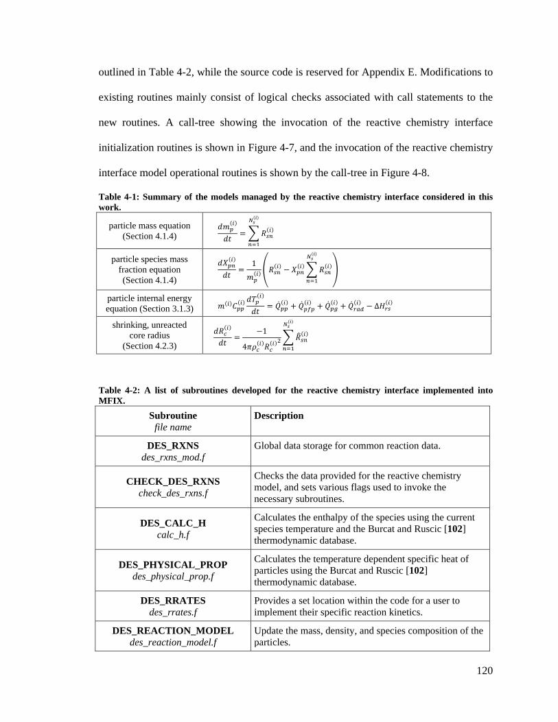
120

outlined in Table 4-2, while the source code is reserved for Appendix E. Modifications to

existing routines mainly consist of logical checks associated with call statements to the

new routines. A call-tree showing the invocation of the reactive chemistry interface

initialization routines is shown in Figure 4-7, and the invocation of the reactive chemistry

interface model operational routines is shown by the call-tree in Figure 4-8.

Table 4-1: Summary of the models managed by the reactive chemistry interface considered in this

work.

particle mass equation

(Section 4.1.4)

particle species mass

fraction equation

(Section 4.1.4)

particle internal energy

equation (Section 3.1.3)

shrinking, unreacted

core radius

(Section 4.2.3)

Table 4-2: A list of subroutines developed for the reactive chemistry interface implemented into

MFIX.

Subroutine

file name

Description

DES_RXNS

des_rxns_mod.f

Global data storage for common reaction data.

CHECK_DES_RXNS

check_des_rxns.f

Checks the data provided for the reactive chemistry

model, and sets various flags used to invoke the

necessary subroutines.

DES_CALC_H

calc_h.f

Calculates the enthalpy of the species using the current

species temperature and the Burcat and Ruscic [102]

thermodynamic database.

DES_PHYSICAL_PROP

des_physical_prop.f

Calculates the temperature dependent specific heat of

particles using the Burcat and Ruscic [102]

thermodynamic database.

DES_RRATES

des_rrates.f

Provides a set location within the code for a user to

implement their specific reaction kinetics.

DES_REACTION_MODEL

des_reaction_model.f

Update the mass, density, and species composition of the

particles.

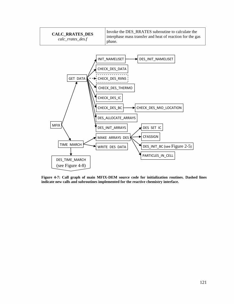
121

CALC_RRATES_DES

calc_rrates_des.f

Invoke the DES_RRATES subroutine to calculate the

interphase mass transfer and heat of reaction for the gas

phase.

Figure 4-7: Call graph of main MFIX-DEM source code for initialization routines. Dashed lines

indicate new calls and subroutines implemented for the reactive chemistry interface.

MFIX

GET_DATA


DES_ALLOCATE_ARRAYS

DES_INIT_ARRAYS

CHECK_DES_DATA

CHECK_DES_THERMO

TIME_MARCH

MAKE_ARRAYS_DES

WRITE_DES_DATA

DES_SET_IC

DES_TIME_MARCH

(see Figure 4-8)

)

CHECK_DES_IC

CHECK_DES_BC CHECK_DES_MIO_LOCATION

DES_INIT_BC (see Figure 2-5)

PARTICLES_IN_CELL

CFASSIGN

CHECK_DES_RXNS

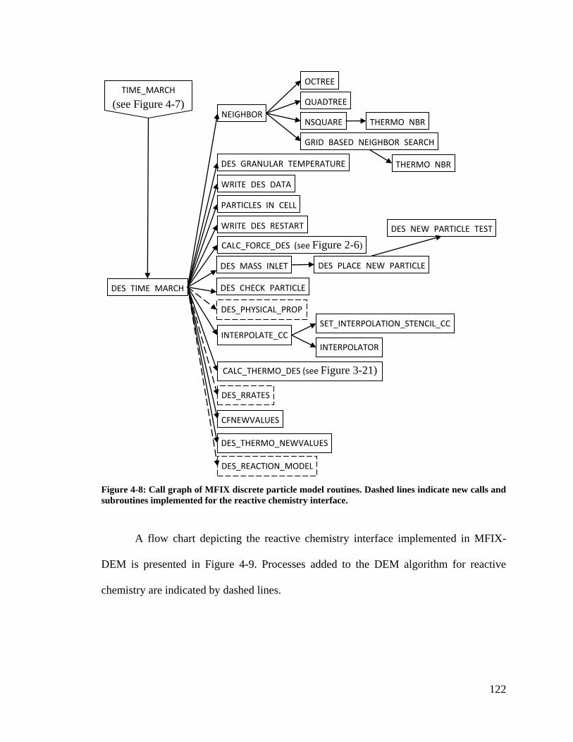
122

Figure 4-8: Call graph of MFIX discrete particle model routines. Dashed lines indicate new calls and

subroutines implemented for the reactive chemistry interface.

A flow chart depicting the reactive chemistry interface implemented in MFIX-

DEM is presented in Figure 4-9. Processes added to the DEM algorithm for reactive

chemistry are indicated by dashed lines.

DES_TIME_MARCH

NEIGHBOR

CFNEWVALUES


WRITE_DES_DATA

PARTICLES_IN_CELL

WRITE_DES_RESTART

CALC_FORCE_DES (see Figure 2-6)

TIME_MARCH

(see Figure 4-7)

INTERPOLATE_CC SET_INTERPOLATION_STENCIL_CC

INTERPOLATOR

CALC_THERMO_DES (see Figure 3-21)


NSQUARE


QUADTREE

OCTREE

THERMO_NBR

THERMO_NBR

DES_MASS_INLET

DES_CHECK_PARTICLE



DES_PHYSICAL_PROP

DES_RRATES

DES_REACTION_MODEL

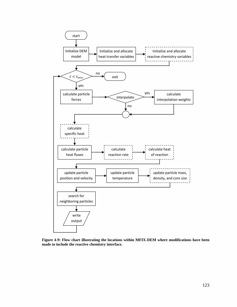
123


made to include the reactive chemistry interface.

Initialize DEM

model


heat transfer variables

calculate particle

forces

update particle


exit

start

no

yes

update particle

temperature

search for


interpolate

no

calculate

interpolation weights

yes

write

output

calculate

reaction rate

calculate heat

of reaction

update particle mass,

density, and core size


reactive chemistry variables

calculate

specific heat

calculate particle

heat fluxes

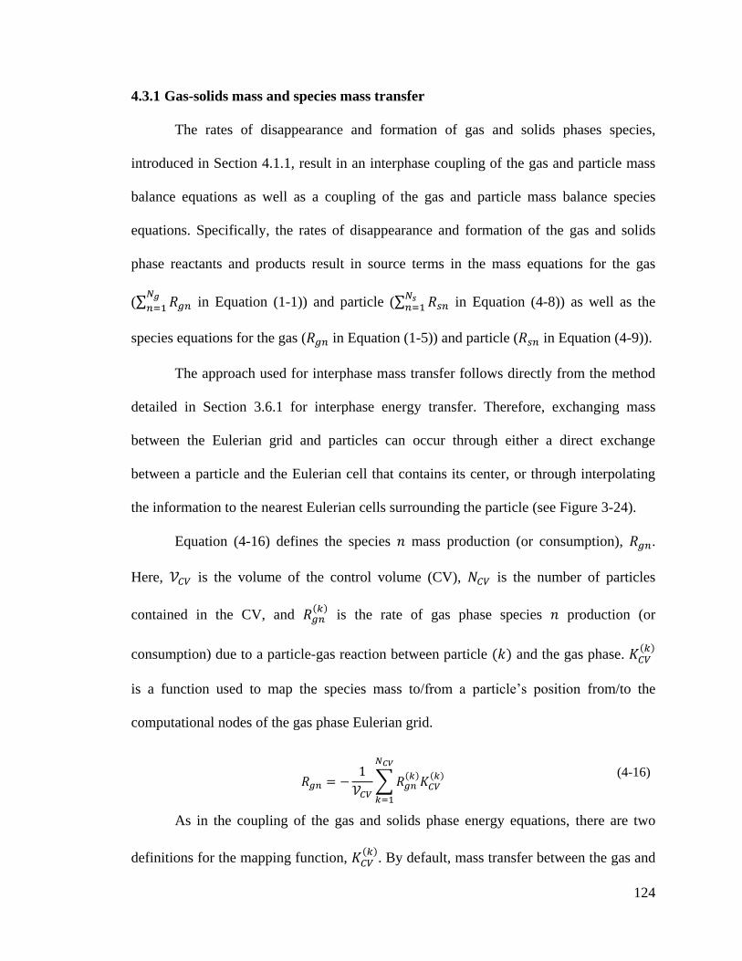
124

4.3.1 Gas-solids mass and species mass transfer

The rates of disappearance and formation of gas and solids phases species,

introduced in Section 4.1.1, result in an interphase coupling of the gas and particle mass

balance equations as well as a coupling of the gas and particle mass balance species

equations. Specifically, the rates of disappearance and formation of the gas and solids

phase reactants and products result in source terms in the mass equations for the gas

(

in Equation (1-1)) and particle ( in Equation (4-8)) as well as the

species equations for the gas ( in Equation (1-5)) and particle ( in Equation (4-9)).

The approach used for interphase mass transfer follows directly from the method

detailed in Section 3.6.1 for interphase energy transfer. Therefore, exchanging mass

between the Eulerian grid and particles can occur through either a direct exchange

between a particle and the Eulerian cell that contains its center, or through interpolating

the information to the nearest Eulerian cells surrounding the particle (see Figure 3-24).

Equation (4-16) defines the species mass production (or consumption), .

Here, is the volume of the control volume (CV), is the number of particles

contained in the CV, and

is the rate of gas phase species production (or

consumption) due to a particle-gas reaction between particle and the gas phase.

is a function used to map the species mass to/from a particle’s position from/to the

computational nodes of the gas phase Eulerian grid.

(4-16)

As in the coupling of the gas and solids phase energy equations, there are two

definitions for the mapping function,

. By default, mass transfer between the gas and

125

a particle is associated with the CV containing the particle’s center (see Figure 3-25-(a)).

A second option distributes mass among the control volumes surrounding the particle via

linear interpolation (see Figure 3-25-(b)). If the interpolation method is employed, the gas

phase species concentrations, if needed by the rate law (see Equation (4-1) in Section

4.1.1), is interpolated to a particle’s position from the surrounding control volumes for

consistency.

The information (mass and species mass) exchanged between the gas and

particles follows the same approach used for energy exchange. The source terms for the

mass and species mass equations for the particles and gas are managed differently to

account for the disjoint updating procedure (see Section 3.6.1). When the gas phase

equations are solved, all of the physical properties of the particles are constant. This is a

direct result of their solutions lagging behind the solution of the gas phase. Similarly,

when the particle phase equations are solved, all of the physical properties of the gas

phase are constant.

4.3.2 Mass, species mass, and core radius updating procedures

As mentioned in the updating procedure for the particle internal energy equation

in Section 3.6.3, there are various methodologies available for solving differential

equations numerically [87,88,89]. However, the time integration methods for the discrete

solids phase momentum equation implemented in MFIX-DEM are limited to Euler’s and

Adams-Bashforth methods [35]. Therefore, the same methods are used to advance the

solution for the particle’s mass, species mass fraction, and core radius equations. Euler’s

method is the default approach selected by this work, and shown for the mass, species

mass fraction, and unreacted core radius in Equations (4-17)-(4-19), respectively. Note

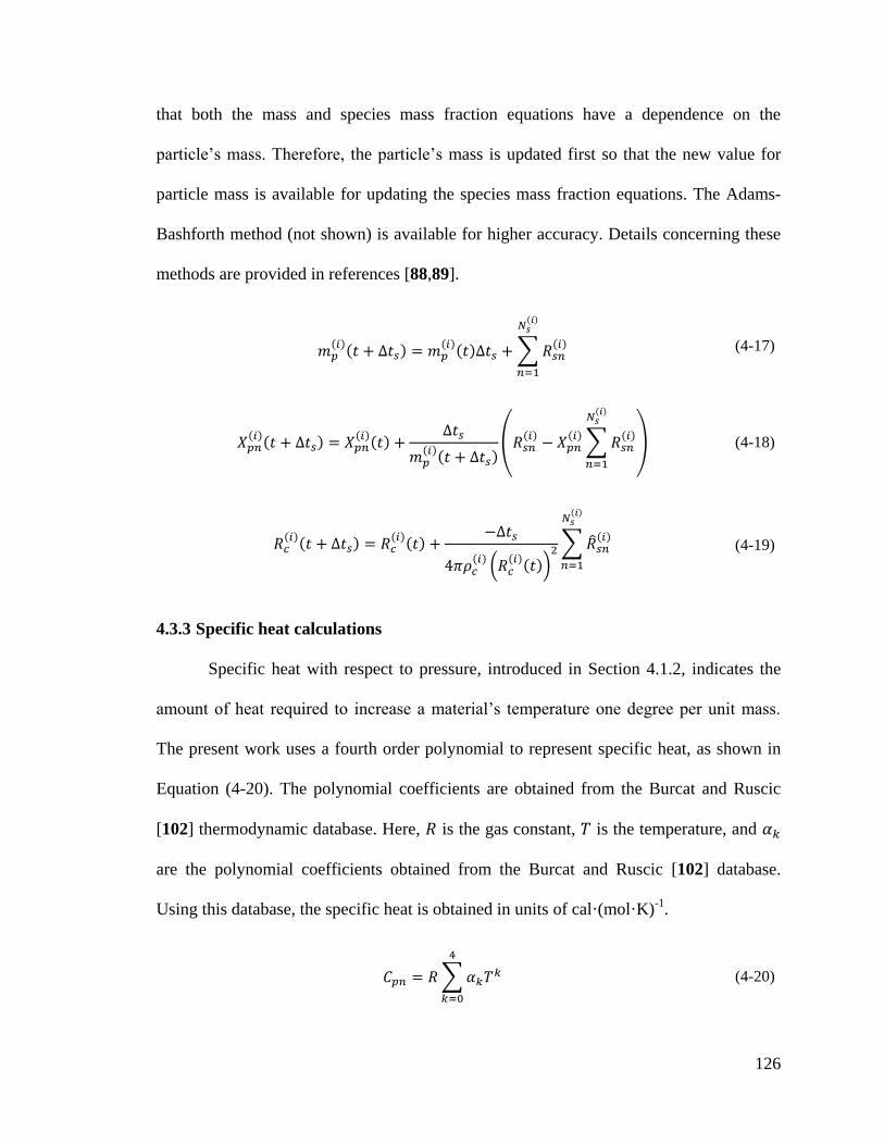
126

that both the mass and species mass fraction equations have a dependence on the

particle’s mass. Therefore, the particle’s mass is updated first so that the new value for

particle mass is available for updating the species mass fraction equations. The Adams-

Bashforth method (not shown) is available for higher accuracy. Details concerning these

methods are provided in references [88,89].

(4-17)

(4-18)

(4-19)

4.3.3 Specific heat calculations

Specific heat with respect to pressure, introduced in Section 4.1.2, indicates the

amount of heat required to increase a material’s temperature one degree per unit mass.

The present work uses a fourth order polynomial to represent specific heat, as shown in

Equation (4-20). The polynomial coefficients are obtained from the Burcat and Ruscic

[102] thermodynamic database. Here, is the gas constant, is the temperature, and

are the polynomial coefficients obtained from the Burcat and Ruscic [102] database.

Using this database, the specific heat is obtained in units of cal·(mol·K)-1

.

(4-20)

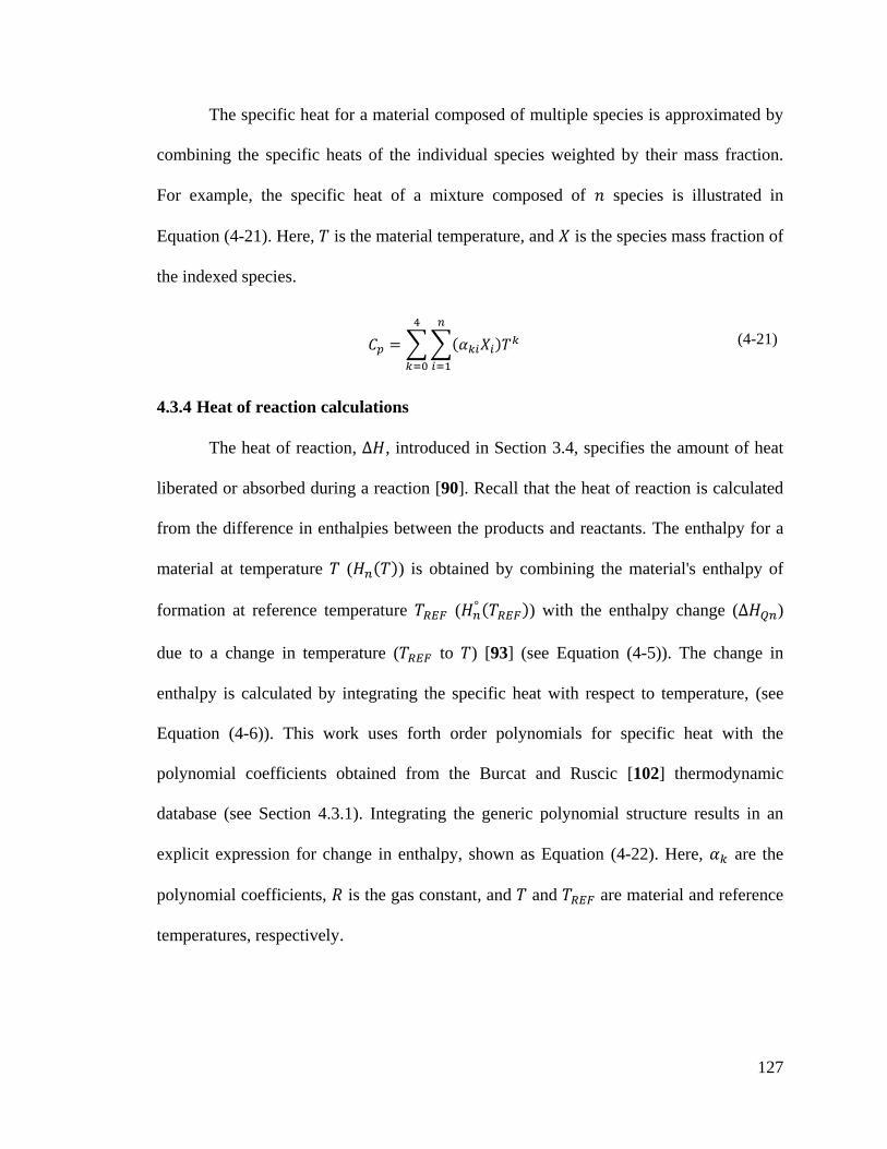
127

The specific heat for a material composed of multiple species is approximated by

combining the specific heats of the individual species weighted by their mass fraction.

For example, the specific heat of a mixture composed of species is illustrated in

Equation (4-21). Here, is the material temperature, and is the species mass fraction of

the indexed species.

(4-21)

4.3.4 Heat of reaction calculations

The heat of reaction, , introduced in Section 3.4, specifies the amount of heat

liberated or absorbed during a reaction [90]. Recall that the heat of reaction is calculated

from the difference in enthalpies between the products and reactants. The enthalpy for a

material at temperature ( ) is obtained by combining the material's enthalpy of

formation at reference temperature ( ) with the enthalpy change ( )

due to a change in temperature ( to ) [93] (see Equation (4-5)). The change in

enthalpy is calculated by integrating the specific heat with respect to temperature, (see

Equation (4-6)). This work uses forth order polynomials for specific heat with the

polynomial coefficients obtained from the Burcat and Ruscic [102] thermodynamic

database (see Section 4.3.1). Integrating the generic polynomial structure results in an

explicit expression for change in enthalpy, shown as Equation (4-22). Here, are the

polynomial coefficients, is the gas constant, and and are material and reference

temperatures, respectively.

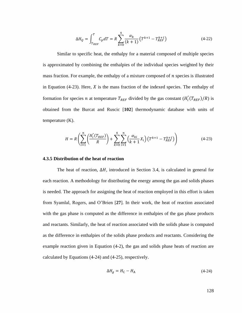
128

(4-22)

Similar to specific heat, the enthalpy for a material composed of multiple species

is approximated by combining the enthalpies of the individual species weighted by their

mass fraction. For example, the enthalpy of a mixture composed of species is illustrated

in Equation (4-23). Here, is the mass fraction of the indexed species. The enthalpy of

formation for species at temperature divided by the gas constant ( ) is

obtained from the Burcat and Ruscic [102] thermodynamic database with units of

temperature (K).

(4-23)

4.3.5 Distribution of the heat of reaction

The heat of reaction, , introduced in Section 3.4, is calculated in general for

each reaction. A methodology for distributing the energy among the gas and solids phases

is needed. The approach for assigning the heat of reaction employed in this effort is taken

from Syamlal, Rogers, and O’Brien [27]. In their work, the heat of reaction associated

with the gas phase is computed as the difference in enthalpies of the gas phase products

and reactants. Similarly, the heat of reaction associated with the solids phase is computed

as the difference in enthalpies of the solids phase products and reactants. Considering the

example reaction given in Equation (4-2), the gas and solids phase heats of reaction are

calculated by Equations (4-24) and (4-25), respectively.

(4-24)

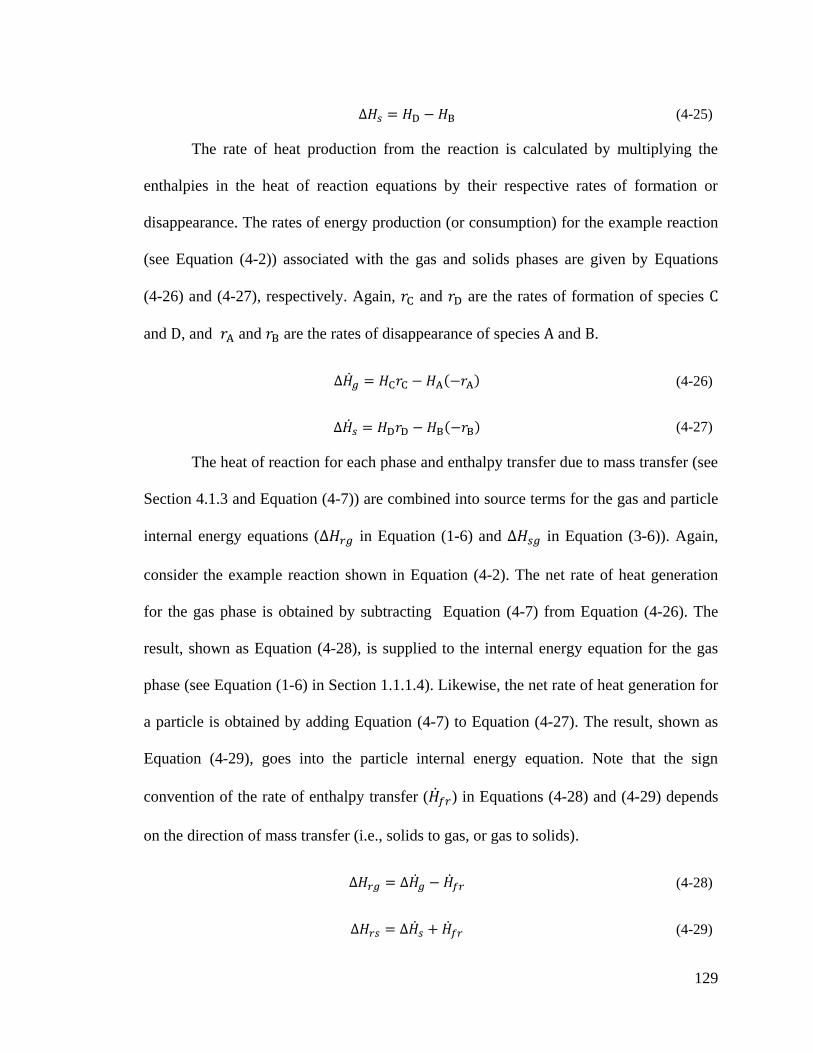
129

(4-25)

The rate of heat production from the reaction is calculated by multiplying the

enthalpies in the heat of reaction equations by their respective rates of formation or

disappearance. The rates of energy production (or consumption) for the example reaction

(see Equation (4-2)) associated with the gas and solids phases are given by Equations

(4-26) and (4-27), respectively. Again, and are the rates of formation of species

and , and and are the rates of disappearance of species and .

(4-26)

(4-27)

The heat of reaction for each phase and enthalpy transfer due to mass transfer (see

Section 4.1.3 and Equation (4-7)) are combined into source terms for the gas and particle

internal energy equations ( in Equation (1-6) and in Equation (3-6)). Again,

consider the example reaction shown in Equation (4-2). The net rate of heat generation

for the gas phase is obtained by subtracting Equation (4-7) from Equation (4-26). The

result, shown as Equation (4-28), is supplied to the internal energy equation for the gas

phase (see Equation (1-6) in Section 1.1.1.4). Likewise, the net rate of heat generation for

a particle is obtained by adding Equation (4-7) to Equation (4-27). The result, shown as

Equation (4-29), goes into the particle internal energy equation. Note that the sign

convention of the rate of enthalpy transfer ( ) in Equations (4-28) and (4-29) depends

on the direction of mass transfer (i.e., solids to gas, or gas to solids).

(4-28)

(4-29)

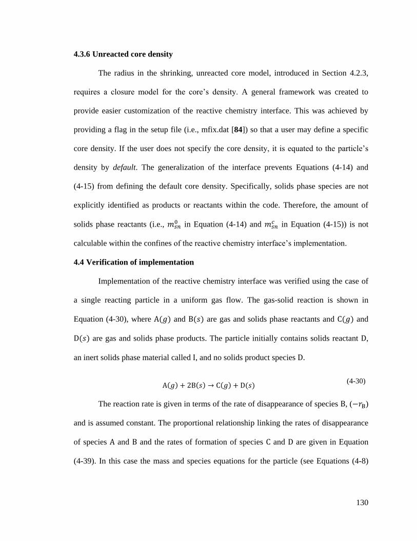
130

4.3.6 Unreacted core density

The radius in the shrinking, unreacted core model, introduced in Section 4.2.3,

requires a closure model for the core’s density. A general framework was created to

provide easier customization of the reactive chemistry interface. This was achieved by

providing a flag in the setup file (i.e., mfix.dat [84]) so that a user may define a specific

core density. If the user does not specify the core density, it is equated to the particle’s

density by default. The generalization of the interface prevents Equations (4-14) and

(4-15) from defining the default core density. Specifically, solids phase species are not

explicitly identified as products or reactants within the code. Therefore, the amount of

solids phase reactants (i.e., in Equation (4-14) and

in Equation (4-15)) is not

calculable within the confines of the reactive chemistry interface’s implementation.

4.4 Verification of implementation

Implementation of the reactive chemistry interface was verified using the case of

a single reacting particle in a uniform gas flow. The gas-solid reaction is shown in

Equation (4-30), where and are gas and solids phase reactants and and

are gas and solids phase products. The particle initially contains solids reactant ,

an inert solids phase material called , and no solids product species .

(4-30)

The reaction rate is given in terms of the rate of disappearance of species , ( )

and is assumed constant. The proportional relationship linking the rates of disappearance

of species and and the rates of formation of species and are given in Equation

(4-39). In this case the mass and species equations for the particle (see Equations (4-8)

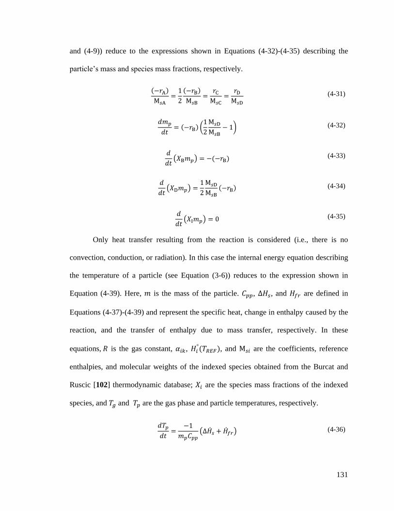
131

and (4-9)) reduce to the expressions shown in Equations (4-32)-(4-35) describing the

particle’s mass and species mass fractions, respectively.

(4-31)

(4-32)

(4-33)

(4-34)

(4-35)

Only heat transfer resulting from the reaction is considered (i.e., there is no

convection, conduction, or radiation). In this case the internal energy equation describing

the temperature of a particle (see Equation (3-6)) reduces to the expression shown in

Equation (4-39). Here, is the mass of the particle. , , and are defined in

Equations (4-37)-(4-39) and represent the specific heat, change in enthalpy caused by the

reaction, and the transfer of enthalpy due to mass transfer, respectively. In these

equations, is the gas constant, , , and are the coefficients, reference

enthalpies, and molecular weights of the indexed species obtained from the Burcat and

Ruscic [102] thermodynamic database; are the species mass fractions of the indexed

species, and and are the gas phase and particle temperatures, respectively.

(4-36)

132

(4-37)

(4-38)

(4-39)

As before, analytic solutions for the particle’s mass, species mass fractions,

temperature, and unreacted core radius are obtained for a particle. All gas phase thermal

and physical properties are assumed constant ( and ). The particle’s specific heat

is assumed constant with respect to temperature. The density of the unreacted core

is calculated from the bulk density of consumable solids phase reactants, given by

Equation (4-15). These assumptions result in five ordinary differential equations solved

by separation of variables. The resulting solutions for the particle’s mass, species mass

fractions, temperature, and unreacted core’s radius are shown in Equations (3-34)-(3-39),

respectively. Here, , , , , and are the particle’s initial mass, species

mass fractions, and temperature, respectively.

(4-40)

(4-41)

133

(4-42)

(4-43)

(4-44)

(4-45)

A simulation employing the same assumptions as defined above was conducted

with MFIX-DEM. The physical and thermodynamic properties of the particle, gas, and

species components are outlined in Table 4-3 and Table 4-4. As the reaction is artificial,

generic values were used for the thermodynamic properties and reaction rate. Realistic

values are not necessary as this verification is designed to test the implementation of the

various models, and not validate any specific chemical reaction. The simulation was run

for 20 seconds of physical time to consume all of the available solids phase reactant

(species ). The solids time step was kept constant at . The

simulation was performed on a single AMD Opteron 265, 1.8GHz processor.

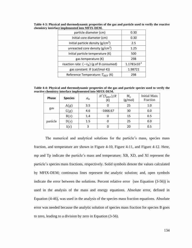
134

Table 4-3: Physical and thermodynamic properties of the gas and particle used to verify the reactive

chemistry interface implemented into MFIX-DEM.

particle diameter (cm) 0.30

Initial core diameter (cm) 0.30

Initial particle density (g/cm3) 2.5

unreacted core density (g/cm3) 1.25

Initial particle temperature (K) 500

gas temperature (K) 298

reaction rate: (g of consumed) 1.1781x10-3

gas constant: (cal/(mol·K)) 1.98721

Reference Temperature: (K) 298

Table 4-4: Physical and thermodynamic properties of the gas and particle species used to verify the

reactive chemistry interface implemented into MFIX-DEM.

Phase Species

(K)

(g/mol) Initial Mass

Fraction

gas 3.5 0 25 1.0

4.6 -1666.67 30 0.0

particle

1.4 0 15 0.5

1.5 0 25 0.0

3 0 20 0.5

The numerical and analytical solutions for the particle’s mass, species mass

fraction, and temperature are shown in Figure 4-10, Figure 4-11, and Figure 4-12. Here,

mp and Tp indicate the particle’s mass and temperature; XB, XD, and XI represent the

particle’s species mass fractions, respectively. Solid symbols denote the values calculated

by MFIX-DEM; continuous lines represent the analytic solution; and, open symbols

indicate the error between the solutions. Percent relative error (see Equation (3-56)) is

used in the analysis of the mass and energy equations. Absolute error, defined in

Equation (4-46), was used in the analysis of the species mass fraction equations. Absolute

error was needed because the analytic solution of species mass fraction for species goes

to zero, leading to a division by zero in Equation (3-56).

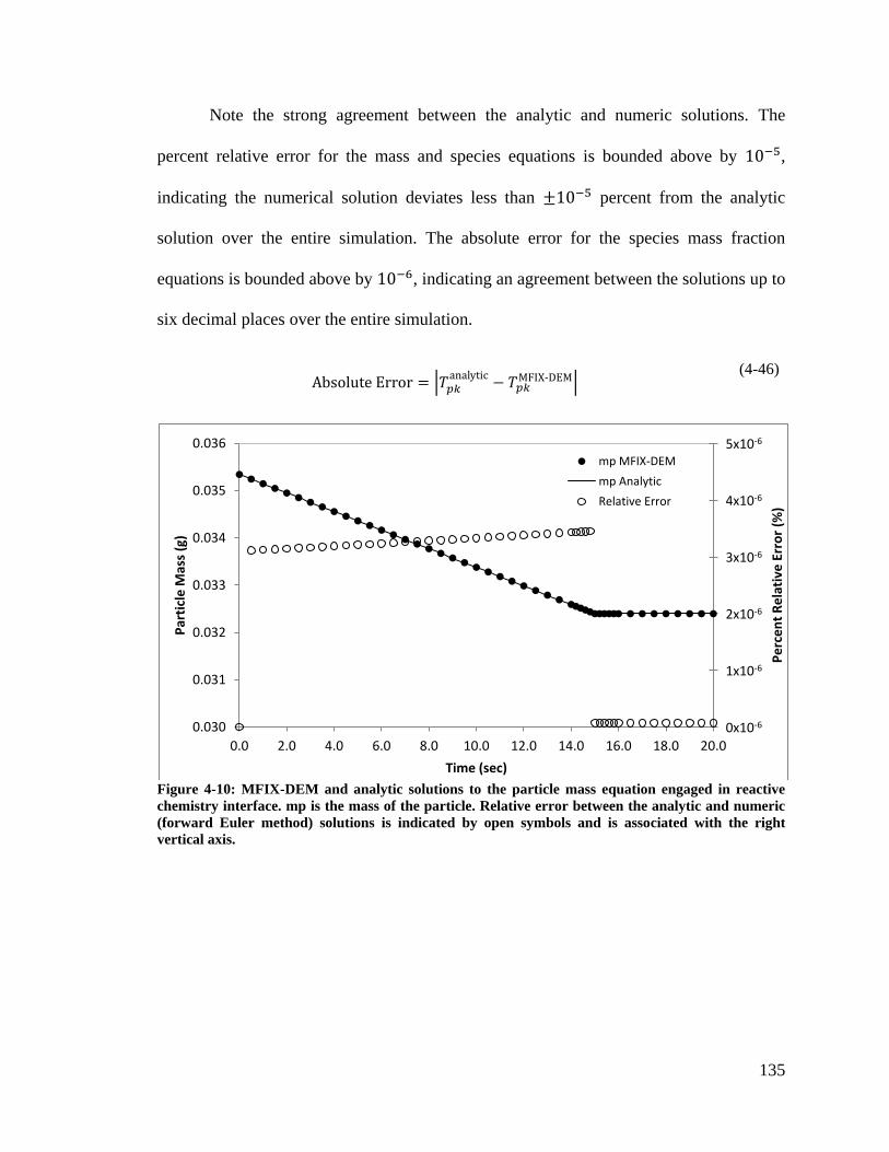
135

Note the strong agreement between the analytic and numeric solutions. The

percent relative error for the mass and species equations is bounded above by ,

indicating the numerical solution deviates less than percent from the analytic

solution over the entire simulation. The absolute error for the species mass fraction

equations is bounded above by , indicating an agreement between the solutions up to

six decimal places over the entire simulation.

(4-46)

Figure 4-10: MFIX-DEM and analytic solutions to the particle mass equation engaged in reactive

chemistry interface. mp is the mass of the particle. Relative error between the analytic and numeric

(forward Euler method) solutions is indicated by open symbols and is associated with the right

vertical axis.

5x10-6

4x10-6

3x10-6

2x10-6

1x10-6

0x10-6 0.030

0.031

0.032

0.033

0.034

0.035

0.036

0.0 2.0 4.0 6.0 8.0 10.0 12.0 14.0 16.0 18.0 20.0

Pe

rce

nt

Re

lati

ve E

rro

r (%

)

Par

ticl

e M

ass

(g)

Time (sec)

mp MFIX-DEM

mp Analytic

Relative Error

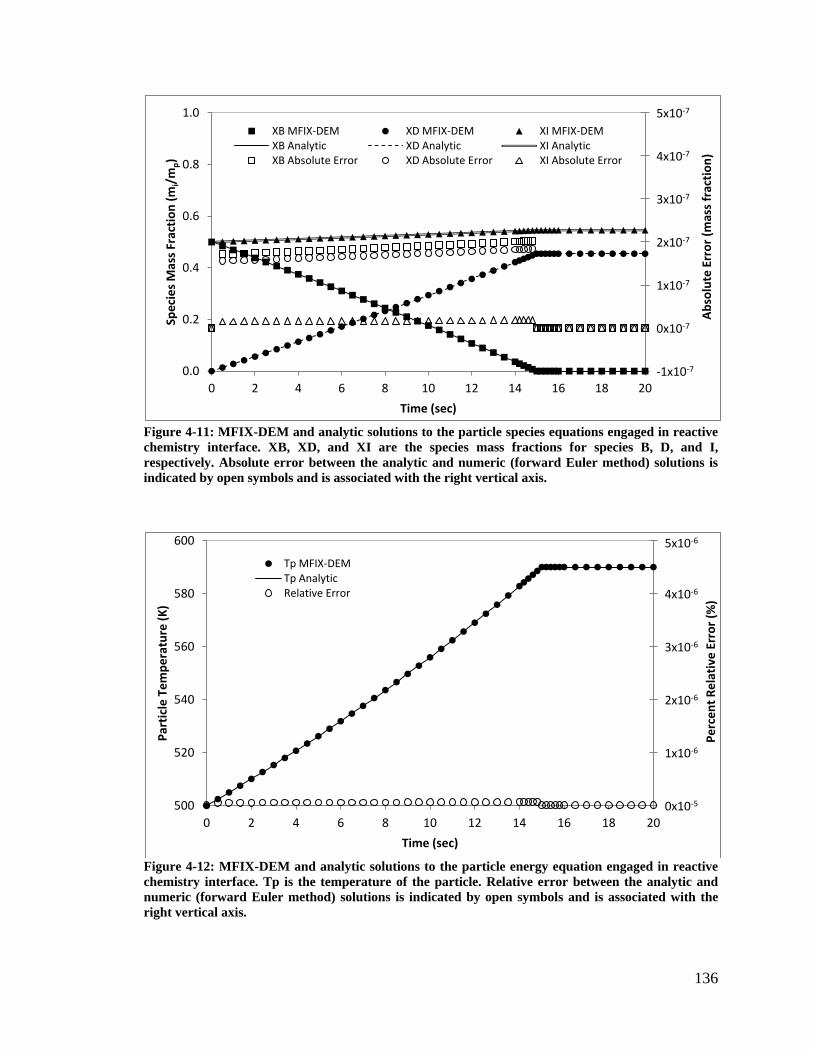
136

Figure 4-11: MFIX-DEM and analytic solutions to the particle species equations engaged in reactive

chemistry interface. XB, XD, and XI are the species mass fractions for species B, D, and I,

respectively. Absolute error between the analytic and numeric (forward Euler method) solutions is

indicated by open symbols and is associated with the right vertical axis.

Figure 4-12: MFIX-DEM and analytic solutions to the particle energy equation engaged in reactive

chemistry interface. Tp is the temperature of the particle. Relative error between the analytic and

numeric (forward Euler method) solutions is indicated by open symbols and is associated with the

right vertical axis.

5x10-7

4x10-7

3x10-7

2x10-7

1x10-7

0x10-7

-1x10-7 0.0

0.2

0.4

0.6

0.8

1.0

0 2 4 6 8 10 12 14 16 18 20

Ab

solu

te E

rro

r (m

ass

frac

tio

n)

Spe

cie

s M

ass

Frac

tio

n (

mi/

mp)

Time (sec)

XB MFIX-DEM XD MFIX-DEM XI MFIX-DEM XB Analytic XD Analytic XI Analytic XB Absolute Error XD Absolute Error XI Absolute Error

5x10-6

4x10-6

3x10-6

2x10-6

1x10-6

0x10-5 500

520

540

560

580

600

0 2 4 6 8 10 12 14 16 18 20

Pe

rce

nt

Re

lati

ve E

rro

r (%

)

Par

ticl

e T

em

pe

ratu

re (

K)

Time (sec)

Tp MFIX-DEM Tp Analytic Relative Error

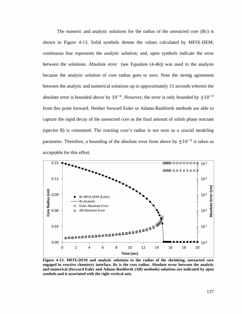
137

The numeric and analytic solutions for the radius of the unreacted core (Rc) is

shown in Figure 4-13. Solid symbols denote the values calculated by MFIX-DEM;

continuous line represents the analytic solution; and, open symbols indicate the error

between the solutions. Absolute error (see Equation (4-46)) was used in the analysis

because the analytic solution of core radius goes to zero. Note the strong agreement

between the analytic and numerical solutions up to approximately 15 seconds wherein the

absolute error is bounded above by . However, the error is only bounded by

from this point forward. Neither forward Euler or Adams-Bashforth methods are able to

capture the rapid decay of the unreacted core as the final amount of solids phase reactant

(species ) is consumed. The reacting core’s radius is not seen as a crucial modeling

parameter. Therefore, a bounding of the absolute error from above by is taken as

acceptable for this effort.

Figure 4-13: MFIX-DEM and analytic solutions to the radius of the shrinking, unreacted core

engaged in reactive chemistry interface. Rc is the core radius. Absolute error between the analytic

and numerical (forward Euler and Adams-Bashforth (AB) methods) solutions are indicated by open

symbols and is associated with the right vertical axis.

10-3

10-4

10-5

10-6

10-7

10-8 0.00

0.03

0.06

0.09

0.12

0.15

0 2 4 6 8 10 12 14 16 18 20

Ab

solu

te E

rro

r (c

m)

Co

re R

adiu

s (c

m)

Time (sec)

Rc MFIX-DEM (Euler)

Rc Analytic

Euler Absolute Error

AB Absolute Error

138

This verification shows a strong agreement between the analytic and numerical

solutions for the mass, species mass fraction, and particle temperature equations.

Similarly, agreement between analytic and numerical solutions for the shrinking,

unreacted core is considered acceptable as it is a non-crucial modeling parameter.

Therefore, the implementation of the reactive chemistry interface into the MFIX-DEM

code is considered successful.

4.5 Closing Remarks

In this chapter, specific concepts of reactive chemistry referenced in this work

was introduced. The subsequent section reviewed the mathematical models describing the

effects of gas-solids reactions on a particle. The shrinking, unreacted core model (see

Section 4.2.3) was selected for its relatively accurate physical account of particle-gas

reactions and ability to account for particles initially containing inert material. Finally,

the implementation of the reactive chemistry interface was verified for a single reacting

particle. Strong agreement was observed between the simulation data and the analytic

solution.

139

Chapter 5: Summary and recommendations

In this effort, MFIX-DEM, an existing CFD-DEM, is enhanced to include discrete

mass inflow-outflow boundary conditions (DMIBC or DMOBC), heat transfer, and an

interface for managing user-defined chemical reactions. The following section provides a

summary of these efforts. This chapter concludes by identifying several areas in which

future work is offered to extend the functionality of the present effort.

5.1 Summary of results

5.1.1 Discrete mass boundary conditions

In Chapter 2, the algorithmic description of discrete mass inflow and outflow

boundary conditions are presented. The inclusion of these functionalities allows models

of more dynamic gas-solids systems by assigning user defined boundary conditions to the

computational domain. An example wherein solids are fed into the bottom of a packed

bed is given. This example illustrates the benefits of using a staging area outside of the

computational domain. In doing so, new particles are fed into a system without disturbing

the overall behavior of pre-existing particles. A second example is provided which

overlaps a DMIBC and gas inflow boundary condition. This demonstrates how additional

modeling flexibility is obtained through defining compound boundary conditions.

5.1.2 Particle heat transfer

Chapter 3 begins by defining the three modes of heat transfer and the internal

energy equation for a single, isothermal particle. An examination of the assumption of

isothermal particles is conducted which indicates that treating the particles as isothermal

is appropriate. In the subsequent sections, an analysis of contact conduction, particle-

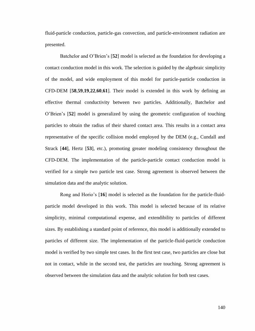
140

fluid-particle conduction, particle-gas convection, and particle-environment radiation are

presented.

Batchelor and O’Brien’s [52] model is selected as the foundation for developing a

contact conduction model in this work. The selection is guided by the algebraic simplicity

of the model, and wide employment of this model for particle-particle conduction in

CFD-DEM [58,59,19,22,60,61]. Their model is extended in this work by defining an

effective thermal conductivity between two particles. Additionally, Batchelor and

O’Brien’s [52] model is generalized by using the geometric configuration of touching

particles to obtain the radius of their shared contact area. This results in a contact area

representative of the specific collision model employed by the DEM (e.g., Cundall and

Strack [44], Hertz [53], etc.), promoting greater modeling consistency throughout the

CFD-DEM. The implementation of the particle-particle contact conduction model is

verified for a simple two particle test case. Strong agreement is observed between the

simulation data and the analytic solution.

Rong and Horio’s [16] model is selected as the foundation for the particle-fluid-

particle model developed in this work. This model is selected because of its relative

simplicity, minimal computational expense, and extendibility to particles of different

sizes. By establishing a standard point of reference, this model is additionally extended to

particles of different size. The implementation of the particle-fluid-particle conduction

model is verified by two simple test cases. In the first test case, two particles are close but

not in contact, while in the second test, the particles are touching. Strong agreement is

observed between the simulation data and the analytic solution for both test cases.

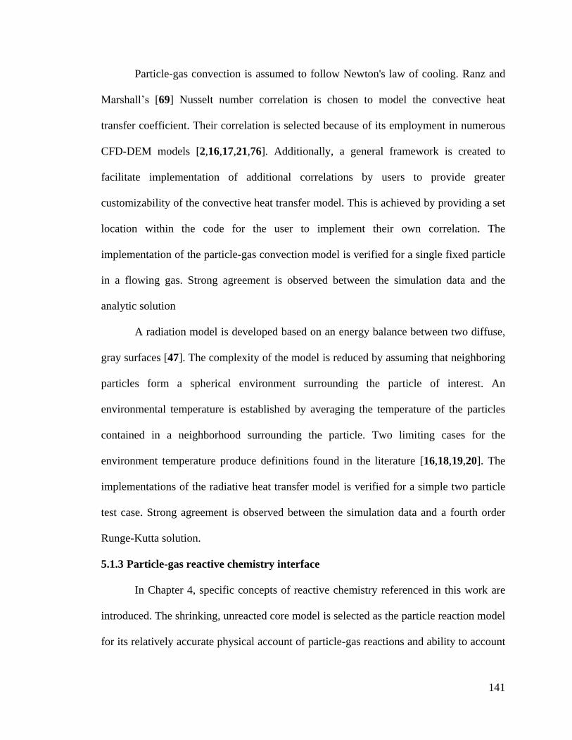
141

Particle-gas convection is assumed to follow Newton's law of cooling. Ranz and

Marshall’s [69] Nusselt number correlation is chosen to model the convective heat

transfer coefficient. Their correlation is selected because of its employment in numerous

CFD-DEM models [2,16,17,21,76]. Additionally, a general framework is created to

facilitate implementation of additional correlations by users to provide greater

customizability of the convective heat transfer model. This is achieved by providing a set

location within the code for the user to implement their own correlation. The

implementation of the particle-gas convection model is verified for a single fixed particle

in a flowing gas. Strong agreement is observed between the simulation data and the

analytic solution

A radiation model is developed based on an energy balance between two diffuse,

gray surfaces [47]. The complexity of the model is reduced by assuming that neighboring

particles form a spherical environment surrounding the particle of interest. An

environmental temperature is established by averaging the temperature of the particles

contained in a neighborhood surrounding the particle. Two limiting cases for the

environment temperature produce definitions found in the literature [16,18,19,20]. The

implementations of the radiative heat transfer model is verified for a simple two particle

test case. Strong agreement is observed between the simulation data and a fourth order

Runge-Kutta solution.

5.1.3 Particle-gas reactive chemistry interface

In Chapter 4, specific concepts of reactive chemistry referenced in this work are

introduced. The shrinking, unreacted core model is selected as the particle reaction model

for its relatively accurate physical account of particle-gas reactions and ability to account

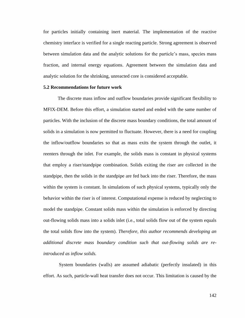
142

for particles initially containing inert material. The implementation of the reactive

chemistry interface is verified for a single reacting particle. Strong agreement is observed

between simulation data and the analytic solutions for the particle’s mass, species mass

fraction, and internal energy equations. Agreement between the simulation data and

analytic solution for the shrinking, unreacted core is considered acceptable.

5.2 Recommendations for future work

The discrete mass inflow and outflow boundaries provide significant flexibility to

MFIX-DEM. Before this effort, a simulation started and ended with the same number of

particles. With the inclusion of the discrete mass boundary conditions, the total amount of

solids in a simulation is now permitted to fluctuate. However, there is a need for coupling

the inflow/outflow boundaries so that as mass exits the system through the outlet, it

reenters through the inlet. For example, the solids mass is constant in physical systems

that employ a riser/standpipe combination. Solids exiting the riser are collected in the

standpipe, then the solids in the standpipe are fed back into the riser. Therefore, the mass

within the system is constant. In simulations of such physical systems, typically only the

behavior within the riser is of interest. Computational expense is reduced by neglecting to

model the standpipe. Constant solids mass within the simulation is enforced by directing

out-flowing solids mass into a solids inlet (i.e., total solids flow out of the system equals

the total solids flow into the system). Therefore, this author recommends developing an

additional discrete mass boundary condition such that out-flowing solids are re-

introduced as inflow solids.

System boundaries (walls) are assumed adiabatic (perfectly insulated) in this

effort. As such, particle-wall heat transfer does not occur. This limitation is caused by the

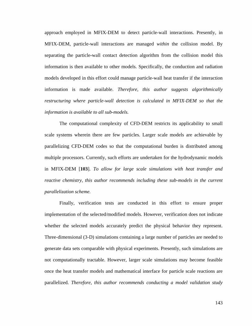
143

approach employed in MFIX-DEM to detect particle-wall interactions. Presently, in

MFIX-DEM, particle-wall interactions are managed within the collision model. By

separating the particle-wall contact detection algorithm from the collision model this

information is then available to other models. Specifically, the conduction and radiation

models developed in this effort could manage particle-wall heat transfer if the interaction

information is made available. Therefore, this author suggests algorithmically

restructuring where particle-wall detection is calculated in MFIX-DEM so that the

information is available to all sub-models.

The computational complexity of CFD-DEM restricts its applicability to small

scale systems wherein there are few particles. Larger scale models are achievable by

parallelizing CFD-DEM codes so that the computational burden is distributed among

multiple processors. Currently, such efforts are undertaken for the hydrodynamic models

in MFIX-DEM [103]. To allow for large scale simulations with heat transfer and

reactive chemistry, this author recommends including these sub-models in the current

parallelization scheme.

Finally, verification tests are conducted in this effort to ensure proper

implementation of the selected/modified models. However, verification does not indicate

whether the selected models accurately predict the physical behavior they represent.

Three-dimensional (3-D) simulations containing a large number of particles are needed to

generate data sets comparable with physical experiments. Presently, such simulations are

not computationally tractable. However, larger scale simulations may become feasible

once the heat transfer models and mathematical interface for particle scale reactions are

parallelized. Therefore, this author recommends conducting a model validation study

144

once the models developed in this effort are incorporated into the current parallelization

scheme.

145

Bibliography

[1] A.H. Pelegrina and G.H. Crapiste, "Modelling the pneumatic drying of food

particles," Journal of Food Engineering, vol. 48, no. 4, pp. 301-310, June 2001.

[2] Yasunobu Kaneko, Takeo Shiojima, and Masayuki Horio, "DEM simulation of

fluidized beds for gas-phase olefin polymerization," Chemical Engineering

Science, vol. 54, pp. 5809-5821, 1999.

[3] D. Geldart, "Types of gas fluidization," Powder Technology, vol. 7, no. 5, pp. 285-

292, May 1973.

[4] R. Krishna and J. M. van Baten, "Using CFD for scaling up gas-solid bubbling

fluidised bed reactors with Geldart A powders," Chemical Engineering Journal,

vol. 82, no. 1-3, pp. 247-257, March 2001.

[5] Sreekanth Pannala, Madhava Syamlal, and Thomas J. O'Brien, Computational Gas-

Solid Flows and Reacting Systems: Theory, Methods, and Practice.: IGI Global,

2010.

[6] Madhava Syamlal, C. Guenther, A. Gel, and S. Pannala, "High performance

computing: Clean coal gasifier designs using hybrid parallelization," in The 13th

International Conference on Fluidization - New Paradigm in Fluidization

Engineering, Gyeong-ju, Korea, May 16-21, 2010.

[7] V. Singh, S. Srivastava, R. Chaval, and V. Vitankar, "Simulation of Gas-Solid

Flow and Design Modifications of Cement Plant Cyclones," in Fifth International

Conference on CFD in the Process Industries CSIRO, Melbourne, Australia, 13-15

December 2006.

[8] B. G.M. van Wachem, J. C. Schouten, C. M. van den Blek, R. Krishna, and J. L.

Sinclair, "Comparative analysis of CFD models of dense gas-solid systems,"

AIChE Journal, vol. 47, no. 5, pp. 1035-1051, May 2001.

[9] Y. Tsuji, T. Tanaka, and T. Ishida, "Lagrangian numerical simulation of plug flow

of cohesionless particles in a horizontal pipe," Powder Technology, vol. 71, no. 3,

pp. 239-250, September 1992.

[10] Y. Tsuji, T. Kawaguchi, and T. Tanaka, "Discrete particle simulation of two-

dimensional fluidized bed," Powder Technology, vol. 77, no. 1, pp. 79-87, October

146

1993.

[11] B. H. Xu and A. B. Yu, "Numerical simulation of the gas-solid flow in a fluidized

bed by combining discrete particle method with computational fluid dynamics,"

Chemical Engineering Science, vol. 52, no. 16, pp. 2785-2809, August 1997.

[12] R. Garg, C. Narayanan, D. Lakehal, and S. Subramaniam, "Accurate numerical

estimation of interphase momentum transfer in Lagrangian-Eulerian simulations of

dispersed two-phase flows," International Journal of Multiphase Flow, vol. 33, no.

12, pp. 1337-1364, December 2007.

[13] Takafumi Mikami, Hidehiro Kamiya, and Masayuki Horio, "Numerical simulation

of cohesive power behavior in a fluidized bed," Chemical Engineering Science, vol.

53, no. 10, pp. 1927-1940, May 1998.

[14] Michael Webber, "Simulation of Cohesive Particle Flows in Granular and Gas-

Solid Systems," University of Colorado, Boulder, PhD Thesis 2004.

[15] Wenqi Zhong, Yuanquan Xiong, Ahulin Yuan, and Mingyao Zang, "DEM

simulation of gas–solid flow behaviors in spout-fluid bed," Chemical Engineering

Science, vol. 61, no. 5, pp. 1571-1584, March 2006.

[16] Degang Rong and Masayuki Horio, "DEM simulation of char combustion in a

fluidized bed," in Second International Conference on CFD in the Minerals and

Process Industries, Melbourne, 1999, pp. 65-70.

[17] J. Li and D.J. Mason, "A computational investigation of transient heat transfer in

pneumatic transport of granular particles," Powder Technology, vol. 112, no. 3, pp.

273-282, October 2000.

[18] Hoasheng Zhou, Gilles Flamant, and Daniel Gauthier, "DEM-LES simulation of

coal combustion in a bubbling fluidized bed part 2: coal combustion at the particle

level," Chemical Engineering Science, vol. 59, no. 20, pp. 4205-4215, October

2004.

[19] Z. Y. Zhou, A. B. Yu, and P. Zulli, "Particle scale study of heat transfer in packed

and bubbling fluidized beds," AIChE Journal, vol. 55, no. 4, pp. 868-884, 2009.

[20] Yongming Geng and Defu Che, "An extended DEM-CFD model for char

combustion in a bubbling fluidized bed combustor of inert sand," Chemical

Engineering Science, vol. 66, no. 2, pp. 207-219, January 2011.

147

[21] Daoyin Liu, Xiaoping Chen, Wu Zhou, and Changsui Zhao, "Simulation of char

and propane combustion in a fluidized bed by extending DEM-CFD approach,"

Proceedings of the Combustion Institute, vol. 33, no. 2, pp. 2701-2708, 2011.

[22] E. Simsek, B. Brosch, S. Wirtz, V. Scherer, and F. Krull, "Numerical simulation of

grate firing systems using a coupled CFD/discrete element method," Powder

Technology, vol. 193, no. 3, pp. 266-273, August 2009.

[23] Michael Oevermann, Stephan Gerber, and Frank Behrendt, "Euler-Lagrange/DEM

simulation of wood gasification in a bubbling fluidized bed reactor," Particuology,

vol. 7, no. 4, pp. 307-316, August 2009.

[24] T. B. Anderson and Roy Jackson, "Fluid mechanical description of fluidized beds.

Equations of motion," Industrial & Engineering Chemistry Fundamentals, vol. 6,

no. 4, pp. 527-539, 1967.

[25] R. Jackson, "Locally averaged equations of motion for a mixture of identical

spherical particles and a Newtonian fluid," Chemical Engineering Science, vol. 52,

no. 15, pp. 2457-2469, August 1997.

[26] Janine Galvin, "On the Hydrodynamic Description of Binary Mixtures of Rapid

Granular Flows and Gas-Fluidized Beds," Department of Chemical and Biological

Engineering, University of Colorado, Boulder, PhD Dissertation 2007.

[27] Madhava Syamlal, William Rogers, and Thomas J. O'Brien, "MFIX

Documentation Theory Guide," U.S. Department of Energy, Morgantown,

Software Documentation December 1993. [Online].

https://www.mfix.org/documentation/Theory.pdf

[28] P. W. Atkins, Physical Chemistry, 2nd ed. Oxford, Great Britain: Oxford

University Press, 1982.

[29] Liang-Shih Fan and Chao Zhu, Principles of Gas-Solid Flows. Cambridge, United

Kingdom: Cambridge University Press, 1998.

[30] Clayton Crowe, Martin Sommerfeld, and Yutaka Tsuji, Multiphase Flows with

Droplets and Particles. Boca Raton, USA: CRC Press, 1998.

[31] G. K. Batchelor, An Introduction to Fluid Dynamics, Reprint edition, Ed.

Cambridge, Great Britain: Cambridge Univ Pr, 1973.

[32] H. K. Versteeg and W. Malalasekera, An introduction to computational fluid

https://www.mfix.org/documentation/Theory.pdf

148

dynamics: The finite volume method. Harlow, England: Pearson Education Limited,

1996.

[33] Dimitri Gidaspow, Multiphase Flow and Fluidization: Continuum and Kinetic

Theory Descriptions, 1st ed. Boston, USA: Academic Press, 1994.

[34] M. P. Allen and D. J. Tildesley, Computer Simulation of Liquids. Oxford, United

Kingdom: Oxford University Press, 1989.

[35] R. Garg, J. Galvin, T. Li, and S. Pannala. (2010, February) Documentation of open-

source MFIX-DEM software for gas-solid flows. From URL

https://mfix.netl.doe.gov/documentation/dem_doc_2010.pdf. [Online].

https://mfix.netl.doe.gov/documentation/dem_doc_2010.pdf

[36] Stefan Luding, "Molecular dynamics simulations of granular materials," in The

Physics of Granular Media. Weinheim, FRG: Wiley-VCH Verlag GmbH & Co.

KGaA, 2005, ch. 13, pp. 299-322.

[37] N. G. Deen, M. Van Sint Annaland, M. A. Van der Hoef, and J. A. M. Kuipers,

"Review of discrete particle modeling of fluidized beds," Chemical Engineering

Science, vol. 62, no. 1-2, pp. 28-44, January 2007.

[38] Pawel Kosinski and Alex C. Hoffmann, "An extension of the hard-sphere particle-

particle collision model to study agglomeration," Chemical Engineering Science,

vol. 65, no. 10, pp. 3231-3239, May 2010.

[39] B. P. B. Hommans, J. A. M. Kuipers, W. J. Briels, and W. P. M. van Swaaij,

"Discrete particle simulation of bubble and slug formation in a two-dimensional

gas-fluidised bed: A hard-sphere approach," Chemical Engineering Science, vol.

51, no. 1, pp. 99-118, January 1996.

[40] Jie Li and J. A. M. Kuipers, "Effect of pressure on gas-solid flow behavior in dense

gas-fluidized beds: a discrete particle simulation study," Powder Technology, vol.

127, no. 2, pp. 173-184, October 2002.

[41] Dhanujay Boyalakuntla, "Simulation of Granular and Gas-Solid Flows using

Discrete Element Method," Carnegie Mellon University, Pittsburgh, PhD Thesis

2003.

[42] H.P. Zhu, Z.Y. Zhou, R.Y. Yang, and A.B. Yu, "Discrete particle simulation of

particulate systems: A review of major applications and findings," Chemical

https://mfix.netl.doe.gov/documentation/dem_doc_2010.pdf

149

Engineering Science, vol. 63, no. 23, pp. 5728-5770, December 2008.

[43] Aytekin Gel, Madhava Syamlal, Sofiane Benyahia, Sreekanth Pannala, and Thomas

J. O'Brien, "Experiences with the open source model for disseminating information

in computational gas-solids flow1-22," in The Fifth World Congress on Particle

Technology, Orlando, Flordia, 2006, pp. 1-22.

[44] P. A. Cundall and O. D. L. Strack, "A discrete numerical model for granular

assemblies," Geotechnique, vol. 29, no. 1, pp. 47-65, March 1979.

[45] Fei Wang, Yu Zhao, Qussai Marashdeh, and Liang-Shih Fan, "Horizontal gas and

gas/solid jet penetration in a gas-solid fluidized bed," Chemical Engineering

Science, vol. 65, no. 11, pp. 3394-3408, June 2010.

[46] Kai Zhang, Jiyu Zhang, and Bijiang Zhang, "Experimental and numerical study of

fluid dynamic parameters in a jetting fluidized bed of a binary mixture," Powder

Technology, vol. 132, no. 1, pp. 30-38, May 2003.

[47] A.F. Mills, Basic Heat & Mass Transfer, 2nd ed.: Prentice Hall, 1998.

[48] M. M. Yovanovich, "Simple explicit expressions for calculation of the Heisler-

Grober charts," in ASME National Heat Transfer Conference, Houston, 1996.

[49] J. Sun and M. M. Chen, "A theoretical analysis of heat transfer due to particle

impact," International Journal of Heat and Mass Transfer, vol. 31, no. 5, pp. 969-

975, May 1988.

[50] Michel Louge, Jamaludin Mohd Yusof, and James T. Jenkins, "Heat transfer in the

pneumatic transport of massive particles," International Journal of Heat and Mass

Transfer, vol. 36, no. 2, pp. 265-275, 1993.

[51] Yoshiyuki Shimizu, "Three-dimensional simulation using fixed coarse-grid

thermal-fluid scheme and conduction heat transfer scheme in distinct element

method," Powder Technology, vol. 165, no. 3, pp. 140-152, July 2006.

[52] G. K. Batchelor and R. W. O'Brien, "Thermal or Electrical Conduction Through a

Granular Material," Proceedings of the Royal Society of London. Series A,

Mathematical and Physical Sciences, vol. 355, no. 1682, pp. 313-333, July 1977.

[53] K. L. Johnson, Contact Mechanics. New York: Cambridge University Press, 1985.

[54] J. H. Zhou, A. B. Yu, and M. Horio, "Finite element modeling of the transient heat

150

conduction between colliding particles," Chemical Engineering Journal, vol. 139,

pp. 510-516, 2008.

[55] H. Zhou, G. Flamant, D. Gauthier, and Y. Flitris, "Simulation of Coal Combustion

in a Bubbling Fluidized Bed by Distinct Element Method," Chemical Engineering

Research and Design, vol. 81, no. 9, pp. 1144-1149, 2003 October, 9th Congress of

the French Society of Chemical Engineering, October 2003.

[56] Itasca Consulting Group, Inc., "PFC2D Version 3.1," Itasca, Minneapolis, Manual

2004.

[57] Itasca Consulting Group, Inc., "PFC3D Version 3.1," Itasca, Minneapolis, Manual

2004.

[58] Watson L. Vargas and J. J. McCarthy, "Heat conduction in granular materials,"

AIChE Journal, vol. 47, no. 5, pp. 1052-1059, May 2001.

[59] F. P. Di Maio, A. Di Renzo, and D. Trevisan, "Comparison of heat transfer models

in DEM-CFD simulations of fluidized beds with an immersed probe," Powder

Technology, vol. 193, no. 3, pp. 257-265, August 2009 2009.

[60] P. A. Moysey and M. R. Thompson, "Modelling the solids inflow and solids

conveying of single-screw extruders using the discrete element method," Powder

Technology, vol. 153, no. 2, pp. 95-107, May 2005.

[61] K. F. Malone and B. H. Xu, "Particle-scale simulation of heat transfer in liquid-

fluidised beds," Powder Technology, vol. 184, no. 2, pp. 189-204, May 2008.

[62] Watson L. Vargas-Escobar, "Discrete Modeling of Heat Conduction in Granular

Media," University of Pittsburg, Pittsburg, PhD Thesis 2002.

[63] C. Y. Wen and T. M. Chang, "Particle-to-particle heat transfer in air-fluidized

beds," in Proceedings of the International symposium on fluidization, Eindhoven,

June 6-9, 1967, pp. 491-505.

[64] C. Delvosalle and J. Vanderschuren, "Gas-to-particle and particle-to-particle heat

transfer in fluidized beds of large particles," Chemical Engineering Science, vol.

40, no. 5, pp. 769-779, 1985.

[65] G. J. Cheng, A. B. Yu, and P. Zulli, "Evaluation of effective thermal conductivity

from the structures of a packed bed," Chemical Engineering Science, vol. 54, pp.

4199-4209, 1999.

151

[66] Jia Wei Chew, Jeffrey R. Wolz, and Christine M. Hrenya, "Axial segregation in

bubbling gas-fluidized beds with Gaussian and lognormal distributions of Geldart

Group B particles," AIChE Journal, vol. 56, no. 12, pp. 3049-3061, December

2010.

[67] A. Mansoori, M. Saffar-Avval, H. Basirat Tabrizi, B. Dabir, and G. Ahmadi, "Inter-

particle heat transfer in a riser of gas-solid turbulent flows," Powder Technology,

vol. 159, no. 1, pp. 35-45, November 2005.

[68] A. M. Xavier and J. F. Davidson, "Heat transfer to surfaces immersed in fluidised

beds, particularly tube arrays," in Fluidization: Proceedings of the Second

Engineering Foundation Conference, Cambridge, England, 2-6 April, 1978, pp.

333-338.

[69] W. E. Ranz and W. R. Marshall, "Evaporation from drops, Part 1 & 2," Chemical

Engineering Progress, vol. 48, pp. 141-146; 173-180, 1952.

[70] P. N. Dwivedi and S. N. Upadhyay, "Particle-fluid mass transfer in fixed and

fluidized beds," Industrial & Engineering Chemistry Process Design and

Development, vol. 16, no. 2, pp. 157-165, April 1977.

[71] D. J. Gunn, "Transfer of heat or mass to particles in fixed and fluidised beds,"

International Journal of Heat and Mass Transfer, vol. 21, no. 4, pp. 467-476, April

1978.

[72] N. Wakao, S. Kaguei, and T. Funazkri, "Effect of fluid dispersion coefficients on

particle-to-fluid heat transfer coefficients in packed beds : Correlation of Nusselt

numbers," Chemical Engineering Science, vol. 34, no. 3, pp. 325-336, 1979.

[73] P. K. Agarwal, "Transport phenomena in multi-particle systems--II. Particle-fluid

heat and mass transfer," Chemical Engineering Science, vol. 43, no. 9, pp. 2501-

2510, 1988.

[74] D. Kunii and O. Levenspiel, Fluidization engineering, 2nd ed. Boston:

Butterworth-Heinemann, 1991.

[75] S. Mankad, K. M. Nixon, and P. J. Fryer, "Measurements of particle-liquid heat

transfer in systems of varied solids fraction," Journal of Food Engineering, vol. 31,

no. 1, pp. 9-33, January 1997.

[76] T. Swasdisevi et al., "Prediction of gas-particle dynamics and heat transfer in a

two-dimensional spouted bed," Advanced Powder Technology, vol. 16, no. 3, pp.

152

275-293, 2005.

[77] Sakae Yagi and Daizo Kunii, "Studies on effective thermal conductivities in packed

beds," AIChE Journal, vol. 3, no. 3, pp. 373-385, September 1957.

[78] John C. Chen, "Heat Transfer," in Handbook of Fluidization and Fluid-Particle

Systems, Wen-Ching Yang, Ed.: CRC Press, 2003.

[79] J. Szekely and Robert J. Fisher, "Bed to wall radiation heat transfer in a gas-solid

fluidized bed," Chemical Engineering Science, vol. 24, no. 5, pp. 833-849, May

1969.

[80] Charles Nelson Zeeb, "Two-Dimensional Radiative Heat Transdfer in Combustion

Gases Via Monte Carlo," Colorado State University, Fort Collins, Thesis 1996.

[81] Z. Mansoori, M. Saffar-Avval, H. Basirat Tabrizi, and G. Ahmad, "Modeling of

heat transfer in turbulent gas–solid flow," International Journal of Heat and Mass

Transfer, vol. 45, no. 6, pp. 1173–1184, March 2002.

[82] Greg F. Naterer, Heat Transfer in Single and Multiphase Systems. Boca Raton:

CRC Press, 2002.

[83] John R. Howell. (2008) A catalog of radiation heat transfer configuration factors.

Document.

[84] MFIX Development Team. (2010, February) Multiphase Flow with Interphase

eXchanges Version MFIX-2010-1 Readme. PDF Document.

[85] Madhava Syamlal, "MFIX Documentation Numerical Technique," U.S.

Department of Energy, Morgantown, Software Documentation 1998.

[86] Sukas V. Patankar, Numerical Heat Transfer and Fluid Flow. USA: McGraw-Hill

Inc., 1980.

[87] Arieh Iserles, A First Course in the Numerical Analysis of Differential Equations.

Cambridge: Cambridge University Press , 1996.

[88] W. H. Press, B. P. Flannery, S. A. Teukoloky, and W. T. Vetterling, Numerical

Recipes in Fortran: The Art of Scientific Computing, 2nd ed.: Cambridge

Univeristy Press, 1992.

[89] David R. Kincaid and E Ward Cheney, Numerical Analysis: Mathematics of

153

Scientific Computing, 3rd ed.: Brooks Cole, 2001.

[90] Octave Levenspiel, Chemical Reaction Engineering, Second Edition ed. New York,

USA: John Wiley & Sons, 1972.

[91] Madhava Syamlal and Thomas J. O’Brien, "Fluid dynamic Simulation of O₂

decomposition in a bubbling fluidized bed," AIChE Journal, vol. 49, no. 11, pp.

2793-2801, November 2003.

[92] Thomas J. B'Brien, Madhava Syamlal, and Chris Guenther, "Computational fluid

dynamic simulations of chemically reactive fluidized bed processes," in Third

International Conference on CFD in the Mineral and Process Industries,

Melbourne, Australia, 2003, pp. 496-474.

[93] H. Scott Fogler, Elements of Chemical Reaction Engineering, 2nd ed. Upper Saddle

River, New Jersey: PRENTICE hALL, 1992.

[94] Julian Szekely, James W. Evans, and Hong Young Sohn, Gas-Solid Reactions.

New York: Academic Press, 1976.

[95] D. C. Dixon, "The definition of reaction rate," Chemical Engineering Science, vol.

25, no. 2, pp. 337-338, February 1970.

[96] Harold C. Weber and Herman P. Meissner, Thermodynamics for Chemical

Engineers, 2nd ed. New York, USA: John Wiley and Sons, 1957.

[97] Richard M. Felder and Ronald W. Rousseau, Elementary Principles of Chemical

Processes, 2nd Edition, Ed. New York: John Wiley and Sons, 1986.

[98] M. Syamlal, "Derivation of Energy Equations in MFIX," U.S. Department of

Energy, Morantown, MFIX Documentation 2007.

[99] Yunus A. Çengel and Michael A. Boles, Thermodynamics: An Engineering

Approach, 4th ed. New York: McGraw-Hill, 2002.

[100] Shunji Homma, Shinji Ogata, Jiro Koga, and Shiro Matsumoto, "Gas-solid reaction

model for a shrinking spherical particle with unreacted shrinking core," Chemical

Engineering Science, vol. 60, no. 18, pp. 4971-4980, September 2005.

[101] T. Bluhm-Drenhaus, E. Simsek, S. Wirtz, and V. Scherer, "A coupled fluid

dynamic-discrete element simulation of heat and mass transfer in a lime shaft kiln,"

Chemical Engineering Science, vol. 9, no. 1, pp. 2821-2834, May 2010.

154

[102] Alexander Burcat and Branko Ruscic. (2005, July) Information Bridge: DOE

Scientific and Technical Information. [Online]. http://www.osti.gov/bridge

[103] Pradeep Gopalakrishnan, "MFIX-DEM Parallelization," in NETL 2011 Workshop

on Multiphase Flow Science, August 16-18, 2011 , Pittsburgh, 2011.

[104] J. Vanderschuren and C. Delvosalle, "Particle-to-particle heat transfer in fluidized

bed drying," Chemical Engineering Science, vol. 35, pp. 1741-1748, 1980.

[105] Kenya Kuwagi, Muhammad Arif Bin Mokhtar, Toshihiro Takami, and Masayuki

Horio, "Analysis of heat transfer between two particles for DEM simulations," in

2007 ECI Conference on the 12th International Conference on Fluidization - New

Horizons in Fluidization Engineering, vol. 4, Vancouver, pp. 241-248.

[106] Y. T. Feng, K. Han, C. F. Li, and D. R. J. Owen, "Discrete thermal element

modelling of heat conduction in particle systems: Basic formulations," Journal of

Computational Physics, vol. 227, pp. 5072-5089, 2008.

[107] J. S. M. Botterill, Fluid-Bed Heat Transfer. New York, New York, United States of

America: Academic Press, 1975.

[108] J. Baeyens, D. van Gauwbergen, and I. Vinckier, "Pneumatic drying: the use of

large-scale experimental data in a design process," Powder Technology, vol. 83, no.

3, pp. 139-148, 1995.

[109] Esmail R. Monazam, Lawrence J. Shadle, Joseph S. Mei, and James Spenik,

"Identification and characteristics of different flow regimes in a circulating

fluidized bed," Powder Technology, vol. 155, no. 1, pp. 17-25, July 2005.

[110] Haosheng Zhou, Gilles Flamant, and Damiel Gauthier, "DEM-LES of coal

combustion in a bubbling fluidized bed. Part I: gas-particle turbulent flow

structure," Chemical Engineering Science, vol. 59, no. 20, pp. 4196-4203, October

2004.

[111] S. Benyahia, M. Syamlal, and T. J. O'Brien. (2008, August) www.mfix.org.

[Online]. https://mfix.netl.doe.gov/documentation/MFIXEquations2005-4-4.pdf

[112] H. Kruggel-Emden, E. Simsek, S. Rickelt, S. Wirtz, and V. Scherer, "Review and

extension of normal force models for the Discrete Element Method," Powder

Technology, vol. 171, no. 3, pp. 157-173, February 2007.

[113] O. Molerus, "Heat transfer in moving beds with a stagnant interstitial gas,"

http://www.osti.gov/bridge

https://mfix.netl.doe.gov/documentation/MFIXEquations2005-4-4.pdf

155

International Journal of Heat and Mass Transfer, vol. 40, no. 17, pp. 4151-4159,

October 1997.

[114] D. Lathouwers and J. Bellan, "Modeling of dense gas-solid reactive mixtures

applied to biomass pyrolysis in a fluidized bed," International Journal of

Multiphase Flow, vol. 27, no. 12, pp. 2155-2187, December 2001.

[115] A. Ingram et al., "Multiple particle tracking in a fluidized bed," in 2007 ECI

Conference on the 12th International Conference on Fluidization - New Horizons

in Fluidization Engineering, Vancouver, 2007, pp. 449-456.

[116] Y. T. Feng, K. Han, and D. R. J. Owen, "Discrete thermal element modelling of

heat conduction in particle systems: Pipe-network model and transient analysis,"

Powder Technology, vol. 193, pp. 248-256, 2009.

[117] Gregory Nellis and Sanford Klein, Heat Transfer. New York, United States of

America: Cambridge niversity Press, 2009.

[118] V. D. Nguyen, C. Cogne, M. Guessasma, E. Bellenger, and J. Fortin, "Discrete

modeling of granular flow with thermal transfer: Application to the discharge of

silos," Applied Thermal Engineering, vol. 29, no. 8-9, pp. 1846-1853, Jume 2009.

[119] M. M. Avedesian and J. F. Davidson, "Combustion of carbon particles in a

fluidised bed," Chemical Engineering Research and Design, vol. 51, pp. 121 - 131,

1973.

[120] M. M. Baum and P. J. Street, "Predicting the combustion behaviour of coal

particles," Combustion Science and Technology, vol. 3, pp. 231-243, 1971.

[121] I. B. Ross and J. F. Davidson, "The combustion of carbon particles in a fluidised

bed," Chemical Engineering Research and Design, vol. 60, pp. 108-114, 1982.

[122] United States Department of Energy, Multiphase Flow with Interphase eXchange,

(Version mfix_05172011_MPPIC_MPI_CutCell) [Open source computer

program]. Available at http://www.mfix.org (Accessed July 11, 2011).

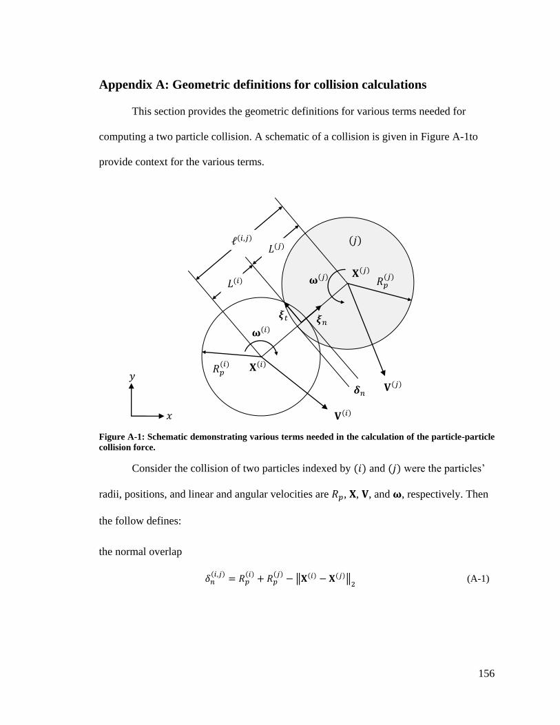
156

Appendix A: Geometric definitions for collision calculations

This section provides the geometric definitions for various terms needed for

computing a two particle collision. A schematic of a collision is given in Figure A-1to

provide context for the various terms.

Figure A-1: Schematic demonstrating various terms needed in the calculation of the particle-particle

collision force.

Consider the collision of two particles indexed by and were the particles’

radii, positions, and linear and angular velocities are , , , and , respectively. Then

the follow defines:

the normal overlap

(A-1)

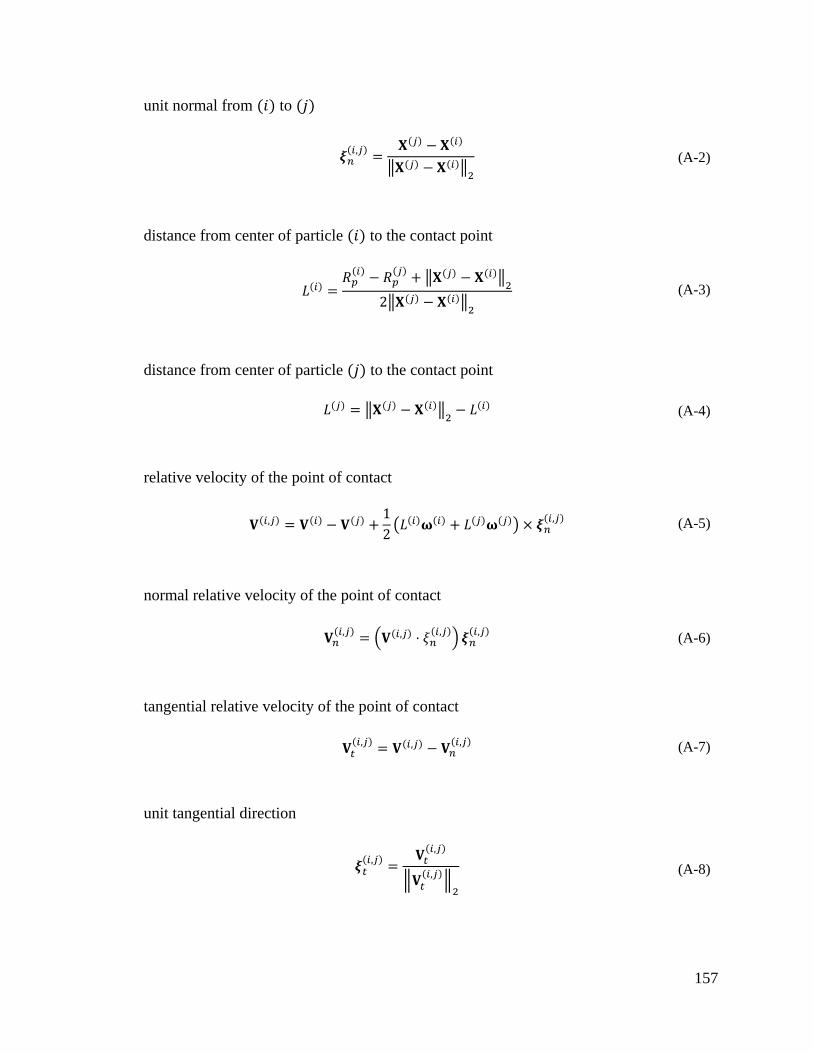
157

unit normal from to

(A-2)

distance from center of particle to the contact point

(A-3)

distance from center of particle to the contact point

(A-4)

relative velocity of the point of contact

(A-5)

normal relative velocity of the point of contact

(A-6)

tangential relative velocity of the point of contact

(A-7)

unit tangential direction

(A-8)

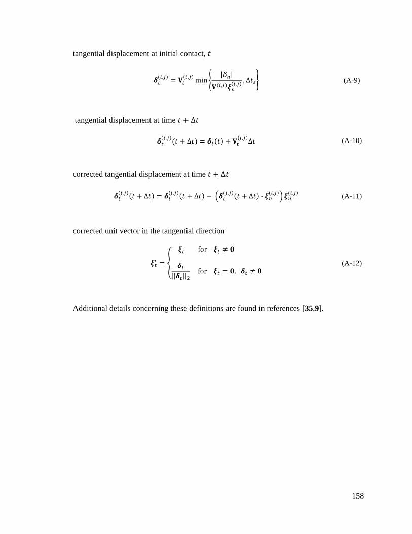
158

tangential displacement at initial contact,

(A-9)

tangential displacement at time

(A-10)

corrected tangential displacement at time

(A-11)

corrected unit vector in the tangential direction

(A-12)

Additional details concerning these definitions are found in references [35,9].

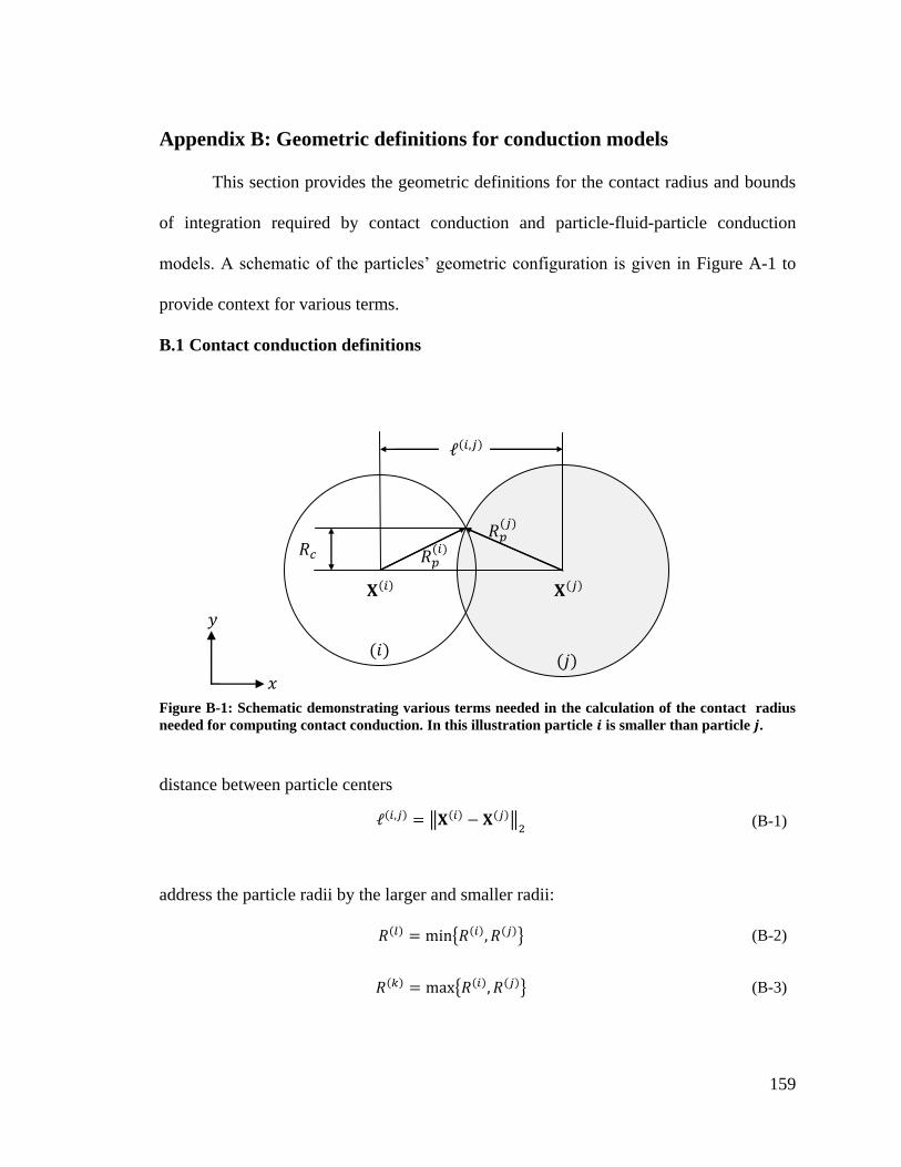
159

Appendix B: Geometric definitions for conduction models

This section provides the geometric definitions for the contact radius and bounds

of integration required by contact conduction and particle-fluid-particle conduction

models. A schematic of the particles’ geometric configuration is given in Figure A-1 to

provide context for various terms.

B.1 Contact conduction definitions

Figure B-1: Schematic demonstrating various terms needed in the calculation of the contact radius

needed for computing contact conduction. In this illustration particle is smaller than particle .

distance between particle centers

(B-1)

address the particle radii by the larger and smaller radii:

(B-2)

(B-3)

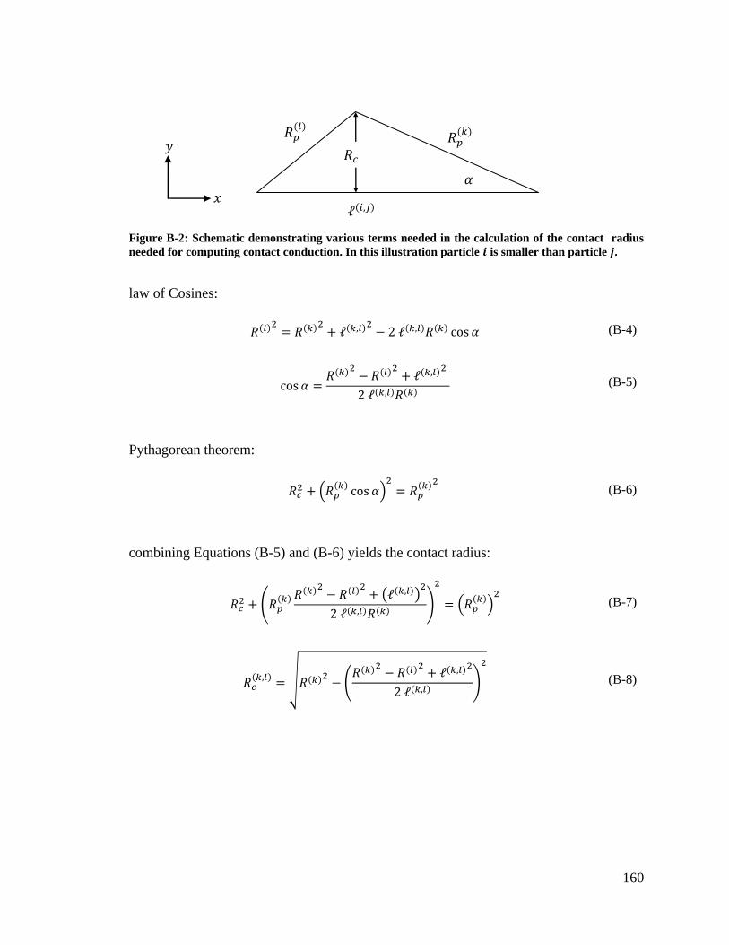
160



law of Cosines:

(B-4)

(B-5)

Pythagorean theorem:

(B-6)

combining Equations (B-5) and (B-6) yields the contact radius:

(B-7)

(B-8)

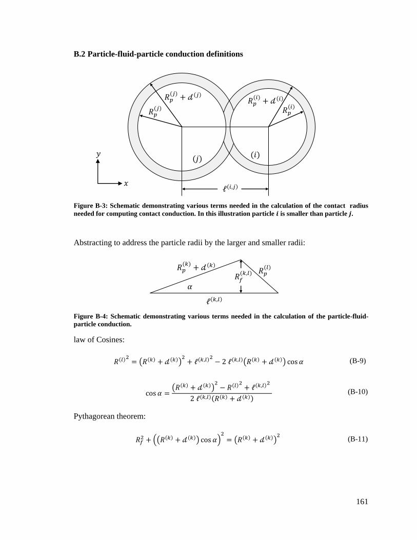
161

B.2 Particle-fluid-particle conduction definitions



Abstracting to address the particle radii by the larger and smaller radii:

Figure B-4: Schematic demonstrating various terms needed in the calculation of the particle-fluid-

particle conduction.

law of Cosines:

(B-9)

(B-10)

Pythagorean theorem:

(B-11)

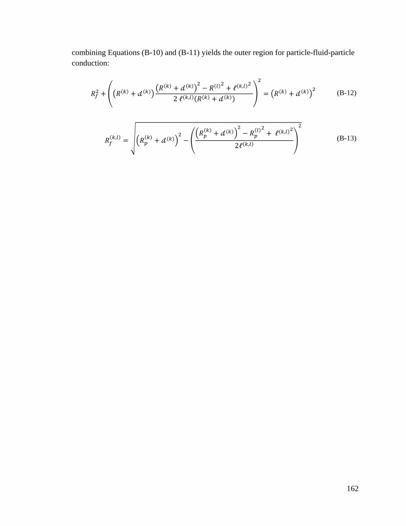
162

combining Equations (B-10) and (B-11) yields the outer region for particle-fluid-particle

conduction:

(B-12)

(B-13)

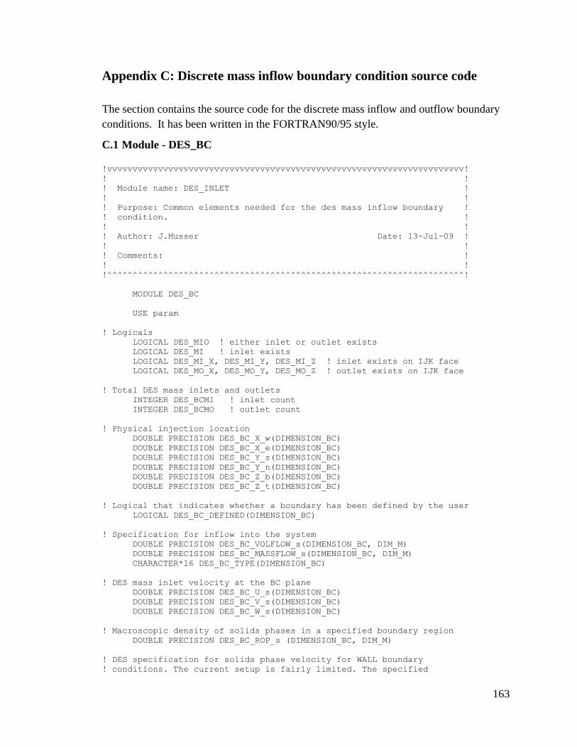
163

Appendix C: Discrete mass inflow boundary condition source code

The section contains the source code for the discrete mass inflow and outflow boundary

conditions. It has been written in the FORTRAN90/95 style.

C.1 Module - DES_BC

!vvvvvvvvvvvvvvvvvvvvvvvvvvvvvvvvvvvvvvvvvvvvvvvvvvvvvvvvvvvvvvvvvvvvvv!

! !

! Module name: DES_INLET !

! !

! Purpose: Common elements needed for the des mass inflow boundary !

! condition. !

! !

! Author: J.Musser Date: 13-Jul-09 !

! !

! Comments: !

! !

!^^^^^^^^^^^^^^^^^^^^^^^^^^^^^^^^^^^^^^^^^^^^^^^^^^^^^^^^^^^^^^^^^^^^^^!

MODULE DES_BC

USE param

! Logicals

LOGICAL DES_MIO ! either inlet or outlet exists

LOGICAL DES_MI ! inlet exists

LOGICAL DES_MI_X, DES_MI_Y, DES_MI_Z ! inlet exists on IJK face

LOGICAL DES_MO_X, DES_MO_Y, DES_MO_Z ! outlet exists on IJK face

! Total DES mass inlets and outlets

INTEGER DES_BCMI ! inlet count

INTEGER DES_BCMO ! outlet count

! Physical injection location

DOUBLE PRECISION DES_BC_X_w(DIMENSION_BC)

DOUBLE PRECISION DES_BC_X_e(DIMENSION_BC)

DOUBLE PRECISION DES_BC_Y_s(DIMENSION_BC)

DOUBLE PRECISION DES_BC_Y_n(DIMENSION_BC)

DOUBLE PRECISION DES_BC_Z_b(DIMENSION_BC)

DOUBLE PRECISION DES_BC_Z_t(DIMENSION_BC)

! Logical that indicates whether a boundary has been defined by the user

LOGICAL DES_BC_DEFINED(DIMENSION_BC)

! Specification for inflow into the system

DOUBLE PRECISION DES_BC_VOLFLOW_s(DIMENSION_BC, DIM_M)

DOUBLE PRECISION DES_BC_MASSFLOW_s(DIMENSION_BC, DIM_M)

CHARACTER*16 DES_BC_TYPE(DIMENSION_BC)

! DES mass inlet velocity at the BC plane

DOUBLE PRECISION DES_BC_U_s(DIMENSION_BC)

DOUBLE PRECISION DES_BC_V_s(DIMENSION_BC)

DOUBLE PRECISION DES_BC_W_s(DIMENSION_BC)

! Macroscopic density of solids phases in a specified boundary region

DOUBLE PRECISION DES_BC_ROP_s (DIMENSION_BC, DIM_M)

! DES specification for solids phase velocity for WALL boundary

! conditions. The current setup is fairly limited. The specified

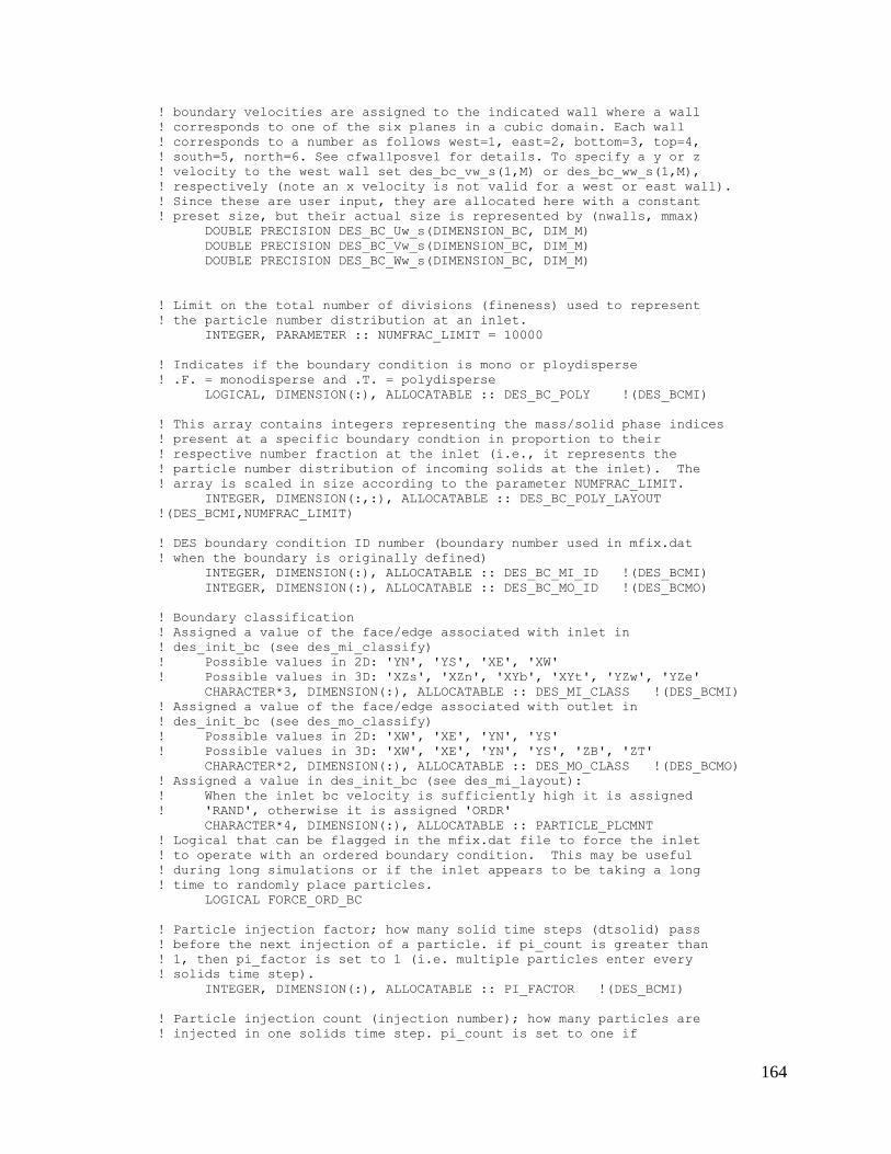
164

! boundary velocities are assigned to the indicated wall where a wall

! corresponds to one of the six planes in a cubic domain. Each wall

! corresponds to a number as follows west=1, east=2, bottom=3, top=4,

! south=5, north=6. See cfwallposvel for details. To specify a y or z

! velocity to the west wall set des_bc_vw_s(1,M) or des_bc_ww_s(1,M),

! respectively (note an x velocity is not valid for a west or east wall).

! Since these are user input, they are allocated here with a constant

! preset size, but their actual size is represented by (nwalls, mmax)

DOUBLE PRECISION DES_BC_Uw_s(DIMENSION_BC, DIM_M)

DOUBLE PRECISION DES_BC_Vw_s(DIMENSION_BC, DIM_M)

DOUBLE PRECISION DES_BC_Ww_s(DIMENSION_BC, DIM_M)

! Limit on the total number of divisions (fineness) used to represent

! the particle number distribution at an inlet.

INTEGER, PARAMETER :: NUMFRAC_LIMIT = 10000

! Indicates if the boundary condition is mono or ploydisperse

! .F. = monodisperse and .T. = polydisperse

LOGICAL, DIMENSION(:), ALLOCATABLE :: DES_BC_POLY !(DES_BCMI)

! This array contains integers representing the mass/solid phase indices

! present at a specific boundary condtion in proportion to their

! respective number fraction at the inlet (i.e., it represents the

! particle number distribution of incoming solids at the inlet). The

! array is scaled in size according to the parameter NUMFRAC_LIMIT.

INTEGER, DIMENSION(:,:), ALLOCATABLE :: DES_BC_POLY_LAYOUT

!(DES_BCMI,NUMFRAC_LIMIT)

! DES boundary condition ID number (boundary number used in mfix.dat

! when the boundary is originally defined)

INTEGER, DIMENSION(:), ALLOCATABLE :: DES_BC_MI_ID !(DES_BCMI)

INTEGER, DIMENSION(:), ALLOCATABLE :: DES_BC_MO_ID !(DES_BCMO)

! Boundary classification

! Assigned a value of the face/edge associated with inlet in

! des_init_bc (see des_mi_classify)

! Possible values in 2D: 'YN', 'YS', 'XE', 'XW'

! Possible values in 3D: 'XZs', 'XZn', 'XYb', 'XYt', 'YZw', 'YZe'

CHARACTER*3, DIMENSION(:), ALLOCATABLE :: DES_MI_CLASS !(DES_BCMI)

! Assigned a value of the face/edge associated with outlet in

! des_init_bc (see des_mo_classify)

! Possible values in 2D: 'XW', 'XE', 'YN', 'YS'

! Possible values in 3D: 'XW', 'XE', 'YN', 'YS', 'ZB', 'ZT'

CHARACTER*2, DIMENSION(:), ALLOCATABLE :: DES_MO_CLASS !(DES_BCMO)

! Assigned a value in des_init_bc (see des_mi_layout):

! When the inlet bc velocity is sufficiently high it is assigned

! 'RAND', otherwise it is assigned 'ORDR'

CHARACTER*4, DIMENSION(:), ALLOCATABLE :: PARTICLE_PLCMNT

! Logical that can be flagged in the mfix.dat file to force the inlet

! to operate with an ordered boundary condition. This may be useful

! during long simulations or if the inlet appears to be taking a long

! time to randomly place particles.

LOGICAL FORCE_ORD_BC

! Particle injection factor; how many solid time steps (dtsolid) pass

! before the next injection of a particle. if pi_count is greater than

! 1, then pi_factor is set to 1 (i.e. multiple particles enter every

! solids time step).

INTEGER, DIMENSION(:), ALLOCATABLE :: PI_FACTOR !(DES_BCMI)

! Particle injection count (injection number); how many particles are

! injected in one solids time step. pi_count is set to one if

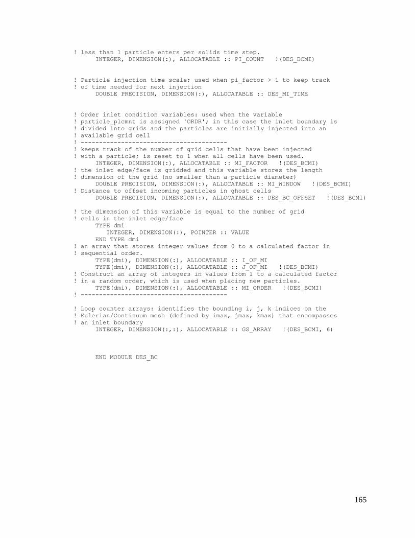
165

! less than 1 particle enters per solids time step.

INTEGER, DIMENSION(:), ALLOCATABLE :: PI_COUNT !(DES_BCMI)

! Particle injection time scale; used when pi_factor > 1 to keep track

! of time needed for next injection

DOUBLE PRECISION, DIMENSION(:), ALLOCATABLE :: DES_MI_TIME

! Order inlet condition variables: used when the variable

! particle_plcmnt is assigned 'ORDR'; in this case the inlet boundary is

! divided into grids and the particles are initially injected into an

! available grid cell

! ----------------------------------------

! keeps track of the number of grid cells that have been injected

! with a particle; is reset to 1 when all cells have been used.

INTEGER, DIMENSION(:), ALLOCATABLE :: MI_FACTOR !(DES_BCMI)

! the inlet edge/face is gridded and this variable stores the length

! dimension of the grid (no smaller than a particle diameter)

DOUBLE PRECISION, DIMENSION(:), ALLOCATABLE :: MI_WINDOW !(DES_BCMI)

! Distance to offset incoming particles in ghost cells

DOUBLE PRECISION, DIMENSION(:), ALLOCATABLE :: DES_BC_OFFSET !(DES_BCMI)

! the dimension of this variable is equal to the number of grid

! cells in the inlet edge/face

TYPE dmi

INTEGER, DIMENSION(:), POINTER :: VALUE

END TYPE dmi

! an array that stores integer values from 0 to a calculated factor in

! sequential order.

TYPE(dmi), DIMENSION(:), ALLOCATABLE :: I_OF_MI

TYPE(dmi), DIMENSION(:), ALLOCATABLE :: J_OF_MI !(DES_BCMI)

! Construct an array of integers in values from 1 to a calculated factor

! in a random order, which is used when placing new particles.

TYPE(dmi), DIMENSION(:), ALLOCATABLE :: MI_ORDER !(DES_BCMI)

! ----------------------------------------

! Loop counter arrays: identifies the bounding i, j, k indices on the

! Eulerian/Continuum mesh (defined by imax, jmax, kmax) that encompasses

! an inlet boundary

INTEGER, DIMENSION(:,:), ALLOCATABLE :: GS_ARRAY !(DES_BCMI, 6)

END MODULE DES_BC

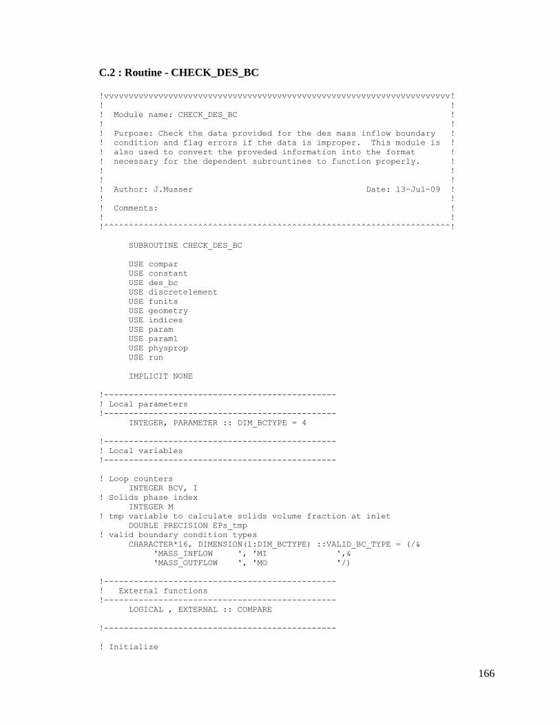
166

C.2 : Routine - CHECK_DES_BC


! !

! Module name: CHECK_DES_BC !

! !

! Purpose: Check the data provided for the des mass inflow boundary !

! condition and flag errors if the data is improper. This module is !

! also used to convert the proveded information into the format !

! necessary for the dependent subrountines to function properly. !

! !

! !


! !

! Comments: !

! !

!^^^^^^^^^^^^^^^^^^^^^^^^^^^^^^^^^^^^^^^^^^^^^^^^^^^^^^^^^^^^^^^^^^^^^^!

SUBROUTINE CHECK_DES_BC

USE compar

USE constant

USE des_bc

USE discretelement

USE funits

USE geometry

USE indices

USE param

USE param1

USE physprop

USE run

IMPLICIT NONE

!-----------------------------------------------

! Local parameters

!-----------------------------------------------

INTEGER, PARAMETER :: DIM_BCTYPE = 4

!-----------------------------------------------

! Local variables

!-----------------------------------------------

! Loop counters

INTEGER BCV, I

! Solids phase index

INTEGER M

! tmp variable to calculate solids volume fraction at inlet

DOUBLE PRECISION EPs_tmp

! valid boundary condition types

CHARACTER*16, DIMENSION(1:DIM_BCTYPE) ::VALID_BC_TYPE = (/&

'MASS_INFLOW ', 'MI ',&

'MASS_OUTFLOW ', 'MO '/)

!-----------------------------------------------

! External functions

!-----------------------------------------------

LOGICAL , EXTERNAL :: COMPARE

!-----------------------------------------------

! Initialize

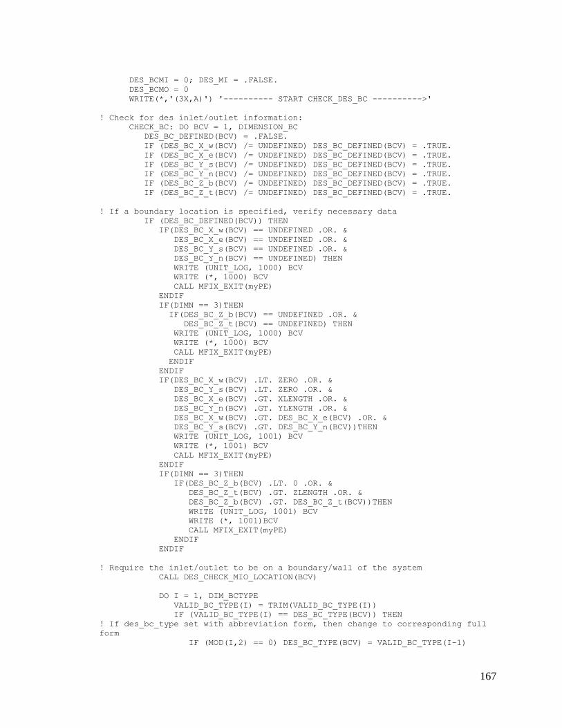
167

DES_BCMI = 0; DES_MI = .FALSE.

DES_BCMO = 0

WRITE(*,'(3X,A)') '---------- START CHECK_DES_BC ---------->'

! Check for des inlet/outlet information:

CHECK_BC: DO BCV = 1, DIMENSION_BC

DES_BC_DEFINED(BCV) = .FALSE.

IF (DES_BC_X_w(BCV) /= UNDEFINED) DES_BC_DEFINED(BCV) = .TRUE.

IF (DES_BC_X_e(BCV) /= UNDEFINED) DES_BC_DEFINED(BCV) = .TRUE.

IF (DES_BC_Y_s(BCV) /= UNDEFINED) DES_BC_DEFINED(BCV) = .TRUE.

IF (DES_BC_Y_n(BCV) /= UNDEFINED) DES_BC_DEFINED(BCV) = .TRUE.

IF (DES_BC_Z_b(BCV) /= UNDEFINED) DES_BC_DEFINED(BCV) = .TRUE.

IF (DES_BC_Z_t(BCV) /= UNDEFINED) DES_BC_DEFINED(BCV) = .TRUE.

! If a boundary location is specified, verify necessary data

IF (DES_BC_DEFINED(BCV)) THEN

IF(DES_BC_X_w(BCV) == UNDEFINED .OR. &

DES_BC_X_e(BCV) == UNDEFINED .OR. &

DES_BC_Y_s(BCV) == UNDEFINED .OR. &

DES_BC_Y_n(BCV) == UNDEFINED) THEN

WRITE (UNIT_LOG, 1000) BCV

WRITE (*, 1000) BCV

CALL MFIX_EXIT(myPE)

ENDIF

IF(DIMN == 3)THEN

IF(DES_BC_Z_b(BCV) == UNDEFINED .OR. &

DES_BC_Z_t(BCV) == UNDEFINED) THEN


WRITE (*, 1000) BCV


ENDIF

ENDIF

IF(DES_BC_X_w(BCV) .LT. ZERO .OR. &

DES_BC_Y_s(BCV) .LT. ZERO .OR. &

DES_BC_X_e(BCV) .GT. XLENGTH .OR. &

DES_BC_Y_n(BCV) .GT. YLENGTH .OR. &

DES_BC_X_w(BCV) .GT. DES_BC_X_e(BCV) .OR. &

DES_BC_Y_s(BCV) .GT. DES_BC_Y_n(BCV))THEN


WRITE (*, 1001) BCV


ENDIF

IF(DIMN == 3)THEN

IF(DES_BC_Z_b(BCV) .LT. 0 .OR. &

DES_BC_Z_t(BCV) .GT. ZLENGTH .OR. &

DES_BC_Z_b(BCV) .GT. DES_BC_Z_t(BCV))THEN


WRITE (*, 1001)BCV


ENDIF

ENDIF

! Require the inlet/outlet to be on a boundary/wall of the system

CALL DES_CHECK_MIO_LOCATION(BCV)

DO I = 1, DIM_BCTYPE

VALID_BC_TYPE(I) = TRIM(VALID_BC_TYPE(I))

IF (VALID_BC_TYPE(I) == DES_BC_TYPE(BCV)) THEN

! If des_bc_type set with abbreviation form, then change to corresponding full

form

IF (MOD(I,2) == 0) DES_BC_TYPE(BCV) = VALID_BC_TYPE(I-1)

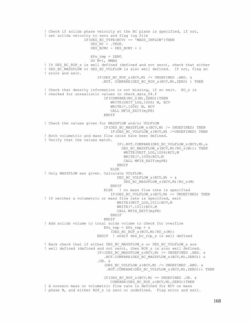
168

! Check if solids phase velocity at the BC plane is specified, if not,

! set solids velocity to zero and flag log file

IF(DES_BC_TYPE(BCV) == 'MASS_INFLOW')THEN

DES_MI = .TRUE.

DES_BCMI = DES_BCMI + 1

EPs_tmp = ZERO

DO M=1, MMAX

! If DES_BC_ROP_s is well defined (defined and not zero), check that either

! DES_BC_MASSFLOW or DES_BC_VOLFLOW is also well defined. If not, flag an

! error and exit.

IF(DES_BC_ROP_s(BCV,M) /= UNDEFINED .AND. &

.NOT. COMPARE(DES_BC_ROP_s(BCV,M),ZERO) ) THEN

! Check that density information is not missing, if so exit. RO_s is

! checked for unrealistic values in check_data_04.f

IF(COMPARE(RO_s(M),ZERO))THEN

WRITE(UNIT_LOG,1006) M, BCV

WRITE(*,1006) M, BCV


ENDIF

! Check the values given for MASSFLOW and/or VOLFLOW

IF(DES_BC_MASSFLOW_s(BCV,M) /= UNDEFINED) THEN

IF(DES_BC_VOLFLOW_s(BCV,M) /=UNDEFINED) THEN

! Both volumetric and mass flow rates have been defined.

! Verify that the values match.

IF(.NOT.COMPARE(DES_BC_VOLFLOW_s(BCV,M),&

DES_BC_MASSFLOW_s(BCV,M)/RO_s(M))) THEN

WRITE(UNIT_LOG,1006)BCV,M

WRITE(*,1006)BCV,M


ENDIF

ELSE

! Only MASSFLOW was given. Calculate VOLFLOW.

DES_BC_VOLFLOW_s(BCV,M) = &

DES_BC_MASSFLOW_s(BCV,M)/RO_s(M)

ENDIF

ELSE ! no mass flow rate is specified

IF(DES_BC_VOLFLOW_s(BCV,M) == UNDEFINED) THEN

! If neither a volumetric or mass flow rate is specified, exit


WRITE(*,1011)BCV,M


ENDIF

ENDIF

! Add solids volume to total solds volume to check for overflow

EPs_tmp = EPs_tmp + &

(DES_BC_ROP_s(BCV,M)/RO_s(M))

ENDIF ! endif des_bc_rop_s is well defined

! Back check that if either DES_BC_MASSFLOW_s or DES_BC_VOLFLOW_s are

! well defined (defined and not zero), then ROP_s is also well defined.

IF((DES_BC_MASSFLOW_s(BCV,M) /= UNDEFINED .AND. &

.NOT.COMPARE(DES_BC_MASSFLOW_s(BCV,M),ZERO)) &

.OR. &

(DES_BC_VOLFLOW_s(BCV,M) /= UNDEFINED .AND. &

.NOT.COMPARE(DES_BC_VOLFLOW_s(BCV,M),ZERO))) THEN

IF(DES_BC_ROP_s(BCV,M) == UNDEFINED .OR. &

COMPARE(DES_BC_ROP_s(BCV,M),ZERO))THEN

! A nonzero mass or volumetric flow rate is defined for BCV on mass

! phase M, and either ROP_s is zero or undefined. Flag error and exit.

169


WRITE(*,1015)BCV, M


ENDIF

ENDIF

ENDDO ! end loop of M=1,MMAX

IF(COMPARE(EPs_tmp,ZERO))THEN

! A des inlet has been defined, but there is no specifed flow information

! (no solids are entering)

WRITE(UNIT_LOG,1013)BCV

WRITE(*,1013)BCV


ELSEIF(EPs_tmp > ONE) THEN

! The total solids volume exceeds one


WRITE(*,1014)BCV


ENDIF

ELSE ! if des_bc_type is not mass_inflow

DES_BCMO = DES_BCMO + 1

ENDIF ! end if des_bc_type is MI, etc

! gives way to exit loop over des_bc_defined(bcv) when valid_bc_type is T

CYCLE CHECK_BC

ENDIF ! endif des_bc_type is valid

ENDDO ! end loop over dim_bc_type

! exit if des_bc_defined but bc_type is not valid

WRITE (UNIT_LOG, 1002) BCV, DES_BC_TYPE(BCV)

WRITE (*, 1002) BCV, DES_BC_TYPE(BCV)

WRITE (UNIT_LOG, 1003) VALID_BC_TYPE

WRITE (*, 1003) VALID_BC_TYPE

WRITE (*, 1008)


ENDIF ! end if des_bc_defined(bcv)

ENDDO CHECK_BC

WRITE(*,1012) DES_BCMI, DES_BCMO

IF(DES_BCMI /= 0 .OR. DES_BCMO /=0)THEN

DES_MIO = .TRUE.

! Allocate necessary arrays for discrete mass inlets

CALL ALLOCATE_DES_MIO(DES_BCMI, DES_BCMO)

! Verify that either the nsquare or grid based neighbor searches are

! used, otherwise flag and exit

IF((DES_NEIGHBOR_SEARCH == 2) .OR. &

(DES_NEIGHBOR_SEARCH == 3)) THEN

WRITE (UNIT_LOG, 1005)

WRITE (*, 1005)


ENDIF

ENDIF

! If the system is started without any particles and an inlet is not

! specified, the run is aborted.

170

IF(DES_BCMI == 0 .AND. PARTICLES == 0)THEN

WRITE(UNIT_LOG, 1009)

WRITE(*, 1009)


ELSEIF(PARTICLES == 0)THEN

WRITE(*,'(5X,A)') &

'Run initiated with no particles in the system'

ENDIF

! Check MAX_PIS requirements

IF(DES_BCMI == 0 .AND. MAX_PIS == UNDEFINED_I)THEN

WRITE(*,'(5X,A)')'Setting MAX_PIS = PARTICLES'

MAX_PIS = PARTICLES

ELSEIF(DES_BCMI /= 0 .AND. MAX_PIS == UNDEFINED_I)THEN


WRITE(*, 1010)


ENDIF

WRITE(*,'(3X,A)') '<---------- END CHECK_DES_BC ----------'

1000 FORMAT(/1X,70('*')//, ' From: CHECK_DES_BC',/, ' Message: ',&

'Insufficient DEM boundary condition infomation',/10X,&

'Check boundary condition number: ',I3,/1X,70('*')/)

1001 FORMAT(/1X,70('*')//, ' From: CHECK_DES_BC',/, ' Messsage: ',&

'Improper DEM boundary condition information',/10X,&

'Check boundary condition number: ',I3,/1X,70('*')/)


'Illegal BC_TYPE for boundary condition ',I3,/10X,&

'BC_TYPE = ',A,' and the valid types are: ')

1003 FORMAT(5X,A16)


A,' not specified in mfix.dat file for BC ',I3,/10X,&

'Setting value to ZERO',/,1X,70('*')/)


'Currently, DEM inlet/outlet only supports the NSQUARE',/10X,&

'and GRID_BASED_NEIGHBOR search methods.',/1X,70('*')/)


'Solids phase ',I3,' is used at DEM boundary condition ',I3,/10X,&

'but its density RO_s is defined as zero.',/1X,70('*')/)


'Both DES_BC_MASSFLOW_s and DES_BC_VOLFOW are defined',/10X,&

'for boundary condition ',I3, ' and solids phase ',I2,&

' but they',/10X, 'are not consistent.',/1X,70('*')/)

1008 FORMAT(/1X,70('*')/)


'The system is initiated with no particles and no DEM',/10X,&

'inlet. The run is being terminated.',/1X,70('*')/)


'If a DEM inlet is specified then the maximum number of',/10X,&

'particles permitted in the system (MAX_PIS) must be set',/10X,&

171

'in mfix.dat',/1X,70('*')/)


'DES_BC_ROP_s is defined (and not zero) for boundary ',/10X,&

'condition ',I3, ' and solids phase ',I2,' without defining',/10X,&

'either DES_BC_MASSFLOW_s or DES_BC_VOLFOW.'/,1X,70('*')/)

1012 FORMAT(5X,'No. of mass inlet BC = ', I4,/,&

5X,'No. of mass outlet BC = ', I4)


'Boundary condition ',I3,' is identifed as an DEM inlet',/10X,&

'but has no associated inflow information. Check mfix.dat',&

/1X,70('*')/)


'The total solids volume fraction for boundary condition',/10X,&

I3,' exceeds one. Check the mfix.dat file.',/1X,70('*')/)


'A nonzero mass or volumetric flow rate has been specified',&

'for',/10X,'boundary condition ', I3, ' and solids phase ',I3,/10X,&

'and the associated DES_BC_ROP_s is either undefined or zero',/10X,&

'Check mfix.dat',/,1X,70('*')/)

RETURN

END SUBROUTINE CHECK_DES_BC

172

C.3 : Routine - DES_CHECK_MIO_LOCATION


! !

! Module name: DES_CHECK_MIO_LOCATION !

! !

! Purpose: This subroutine verifies that the location of the DES mass !

! inlet/outlet was specified to on a wall of the system. If an inlet !

! or outlet is located elsewhere, an error is flagged and the program !

! terminated. !

! !

! Author: J.Musser Date: 17-Aug-09 !

! !

! Comments: !

! !

!^^^^^^^^^^^^^^^^^^^^^^^^^^^^^^^^^^^^^^^^^^^^^^^^^^^^^^^^^^^^^^^^^^^^^^!

SUBROUTINE DES_CHECK_MIO_LOCATION(BCV)

USE compar

USE constant

USE des_bc

USE discretelement

USE funits

USE geometry

USE param1

USE physprop

USE run

!-----------------------------------------------

! Local variables

!-----------------------------------------------

INTEGER BCV ! Boundary Condition

!-----------------------------------------------

IF(DIMN == 2) THEN

! Check verticle mass inlet

IF(DES_BC_X_w(BCV) == DES_BC_X_e(BCV)) THEN

IF(DES_BC_X_w(BCV) /= ZERO .AND. &

DES_BC_X_w(BCV) /= XLENGTH)THEN

WRITE (UNIT_LOG, 1100)BCV; WRITE (*, 1100)BCV


ENDIF

ENDIF

! Check horizontal mass inlet

IF(DES_BC_Y_s(BCV) == DES_BC_Y_n(BCV)) THEN

IF(DES_BC_Y_s(BCV) /= ZERO .AND. &

DES_BC_Y_s(BCV) /= YLENGTH)THEN



ENDIF

ENDIF

! Require the inlet be an edge in 2D not a point

IF(DES_BC_X_w(BCV) == DES_BC_X_e(BCV) .AND. &

DES_BC_Y_s(BCV) == DES_BC_Y_n(BCV)) THEN

WRITE (UNIT_LOG, 1101)&

'DES mass inlet/outlet must larger than a single point.',BCV

WRITE (*, 1101)&



ENDIF

! Require the inlet be an edge in 2D not a plane

173

IF(DES_BC_X_w(BCV) /= DES_BC_X_e(BCV) .AND. &

DES_BC_Y_s(BCV) /= DES_BC_Y_n(BCV)) THEN


'For DIMN=2, DES mass inlet/outlet cannot be an area.',BCV

WRITE (*, 1101)&

'For DIMN=2, DES mass inlet/outlet cannot be an area.',BCV


ENDIF

ELSE ! if dimn != 2


IF(DES_BC_X_w(BCV) /= ZERO .AND. DES_BC_X_w(BCV) /= XLENGTH)THEN


! Require the inlet be a slit/edge on the XZ-face





ENDIF

ENDIF

IF(DES_BC_Z_b(BCV) == DES_BC_Z_t(BCV)) THEN

! Require the inlet be a slit/edge on the XY-face

IF(DES_BC_Z_b(BCV) /= ZERO .AND. &

DES_BC_Z_b(BCV) /= ZLENGTH)THEN



ENDIF

ENDIF

! Require an area inlet to be on the YZ-face and the face must be at

! one of the x-boundary edges

IF(DES_BC_Y_s(BCV) /= DES_BC_Y_n(BCV) .AND. &

DES_BC_Z_b(BCV) /= DES_BC_Z_t(BCV)) THEN



ENDIF

ENDIF

ENDIF


IF(DES_BC_Y_s(BCV) /= ZERO .AND. DES_BC_Y_s(BCV) /= YLENGTH)THEN


! Require the inlet be a slit/edge on the YZ-face





ENDIF

ENDIF


! Require the inlet be a slit/edge on the XY-face

IF(DES_BC_Z_b(BCV) /= ZERO .AND. &




ENDIF

ENDIF


DES_BC_Z_b(BCV) /= DES_BC_Z_t(BCV)) THEN

! Require an area inlet to be on the XZ-face and the face must be at

! one of the y-boundary edges



174

ENDIF

ENDIF

ENDIF


IF(DES_BC_Z_b(BCV) /= ZERO .AND. DES_BC_Z_b(BCV) /= ZLENGTH)THEN


! Require the inlet be a slit/edge on the YZ-face





ENDIF

ENDIF


! Require the inlet be a slit/edge on the XZ-face





ENDIF


DES_BC_Y_s(BCV) /= DES_BC_Y_n(BCV)) THEN

! Require an area inlet to be on the XY-face and the face must be at

! one of the z-boundary edges



ENDIF

ENDIF

ENDIF

ENDIF

ENDIF ! end if dimn == 2 / else

! The following checks target potential bc problems in 3D systems

! ----------------------------------------


DES_BC_Y_s(BCV) == DES_BC_Y_n(BCV) .AND. &

DES_BC_Z_b(BCV) == DES_BC_Z_t(BCV))THEN

! Prohibit point-based mass inlet



WRITE (*, 1101)&



ENDIF


DES_BC_Y_s(BCV) /= DES_BC_Y_n(BCV) .AND. &

DES_BC_Z_b(BCV) /= DES_BC_Z_t(BCV))THEN

! Prohibit volume-based mass inlet


'For DIMN=3, DES mass inlet/outlet cannot be a volume.',BCV

WRITE (*, 1101)&

'For DIMN=3, DES mass inlet/outlet cannot be a volume.',BCV


ENDIF

IF((DES_BC_X_w(BCV) == DES_BC_X_e(BCV) .AND. &


((DES_BC_X_w(BCV) == ZERO .AND. DES_BC_Y_s(BCV) == ZERO) &

.OR. (DES_BC_X_w(BCV) == ZERO .AND. DES_BC_Y_s(BCV) == YLENGTH) &

.OR. (DES_BC_X_w(BCV) == XLENGTH .AND. DES_BC_Y_s(BCV) == ZERO) &

175

.OR. (DES_BC_X_w(BCV) == XLENGTH .AND. DES_BC_Y_s(BCV) == YLENGTH)))

.OR. &

(DES_BC_X_w(BCV) == DES_BC_X_e(BCV) .AND. &

DES_BC_Z_b(BCV) == DES_BC_Z_t(BCV) .AND. &

((DES_BC_X_w(BCV) == ZERO .AND. DES_BC_Z_b(BCV) == ZERO) &

.OR. (DES_BC_X_w(BCV) == ZERO .AND. DES_BC_Z_b(BCV) == ZLENGTH) &

.OR. (DES_BC_X_w(BCV) == XLENGTH .AND. DES_BC_Z_b(BCV) == ZERO) &

.OR. (DES_BC_X_w(BCV) == XLENGTH .AND. DES_BC_Z_b(BCV) == ZLENGTH)))

.OR. &

(DES_BC_Y_s(BCV) == DES_BC_Y_n(BCV) .AND. &


((DES_BC_Y_s(BCV) == ZERO .AND. DES_BC_Z_b(BCV) == ZERO) &

.OR. (DES_BC_Y_s(BCV) == ZERO .AND. DES_BC_Z_b(BCV) == ZLENGTH) &

.OR. (DES_BC_Y_s(BCV) == YLENGTH .AND. DES_BC_Z_b(BCV) == ZERO) &

.OR. (DES_BC_Y_s(BCV) == YLENGTH .AND. DES_BC_Z_b(BCV) ==

ZLENGTH))))THEN

! Prohibit DES mass inlet along domain edges


'DES mass inlet/outlet cannot be positioned in a corner.',BCV

WRITE (*, 1101)&

'DES mass inlet/outlet cannot be positioned in a corner.',BCV


ENDIF

1100 FORMAT(/1X,70('*')//, ' From: DES_CHECK_MIO_LOCATION',/10X,&

' Message: DES boundary condition ',I4, ' must be ',/10X,&

' specified on a wall.',/1X,70('*'))

1101 FORMAT(/1X,70('*')//, ' From: DES_CHECK_MIO_LOCATION',/10X,&

' Message: ',A, /10X,'Check boundary condition ',I4,&

' in mfix.dat.',/1X,70('*'))

RETURN

END SUBROUTINE DES_CHECK_MIO_LOCATION

176

C.4 : Routine - ALLOCATE_DES_MIO


! !

! Module name: ALLOCATE_DES_MIO !

! !

! Purpose: !

! !


! !

! Comments: !

! !

!^^^^^^^^^^^^^^^^^^^^^^^^^^^^^^^^^^^^^^^^^^^^^^^^^^^^^^^^^^^^^^^^^^^^^^!

SUBROUTINE ALLOCATE_DES_MIO

USE des_bc

USE discretelement

IMPLICIT NONE

!-----------------------------------------------

! Local variables

!-----------------------------------------------

INTEGER I ! Loop counter for no. of DES_BCMI

!-----------------------------------------------

! Allocate/Initialize for inlets

IF(DES_BCMI /= 0)THEN

! Boundary condition ID array

Allocate( DES_BC_MI_ID (DES_BCMI) )

! Distance offset of incoming particles in ghost cell

Allocate( DES_BC_OFFSET (DES_BCMI) )

! Particle injection factor

Allocate( PI_FACTOR (DES_BCMI) )

! Particle injection count (injection number)

Allocate( PI_COUNT (DES_BCMI) )

! Particle injection time scale

Allocate( DES_MI_TIME (DES_BCMI) )


Allocate( DES_MI_CLASS (DES_BCMI) )

Allocate( PARTICLE_PLCMNT (DES_BCMI) )

! Order inlet condition variables

! (only needed if particle_plcmt is assigned 'ordr')

Allocate( MI_FACTOR (DES_BCMI) )

Allocate( MI_WINDOW (DES_BCMI) )

Allocate( MI_ORDER (DES_BCMI) ) ! type dmi

Allocate( I_OF_MI ( DES_BCMI) ) ! type dmi

Allocate( J_OF_MI ( DES_BCMI) ) ! type dmi

! Grid search loop counter array; 6 = no. of faces

Allocate( GS_ARRAY (DES_BCMI, 6) )

! Logical array stating if a bounday condition is polydisperse

177

Allocate( DES_BC_POLY( DES_BCMI ) )

! Array used for polydisperse inlets: stores the particle number

! distribution of an inlet scaled with numfrac_limit

Allocate( DES_BC_POLY_LAYOUT( DES_BCMI, NUMFRAC_LIMIT ) )

! Initializiation

! Logical for whether inlet is polydisperse

DES_BC_POLY(:) = .FALSE.

! Logical for inlet existance on IJK face

DES_MI_X = .FALSE.

DES_MI_Y = .FALSE.

DES_MI_Z = .FALSE.

! Integer arrays

DES_BC_MI_ID(:) = -1

PI_FACTOR(:) = -1

PI_COUNT(:) = -1

MI_FACTOR(:) = -1

MI_WINDOW(:) = -1

GS_ARRAY(:,:) = -1

DES_BC_POLY_LAYOUT(:,:) = -1

! Double precision arrays

DES_MI_TIME(:) = UNDEFINED

! Character precision arrays

DES_MI_CLASS(:) = UNDEFINED_C

PARTICLE_PLCMNT(:) = UNDEFINED_C

! Derived data types

DO I = 1,DES_BCMI

NULLIFY( MI_ORDER(I)%VALUE )

NULLIFY( I_OF_MI(I)%VALUE )

NULLIFY( J_OF_MI(I)%VALUE )

ENDDO

ENDIF ! end if des_bcmi /= 0

! Allocate/Initialize for outlets

IF(DES_BCMO /= 0)THEN

! Boundary Condition ID array

Allocate( DES_BC_MO_ID (DES_BCMO) )


Allocate( DES_MO_CLASS (DES_BCMO) )

! Initializiation

! Integer arrays

DES_BC_MO_ID(:) = -1

! Character arrays

DES_MO_CLASS(:) = UNDEFINED_C

! Logical for outlet existance on IJK face

DES_MO_X = .FALSE.

DES_MO_Y = .FALSE.

DES_MO_Z = .FALSE.

ENDIF ! end if des_bcmo /= 0

RETURN

END SUBROUTINE ALLOCATE_DES_MIO

178

C.5 : Routine - DES_INIT_BC


! !

! Module name: DES_INIT_BC !

! !

! !

! !

! Author: J.Musser Date: 23-Nov-09 !

! !

! Comments: !

! !

!^^^^^^^^^^^^^^^^^^^^^^^^^^^^^^^^^^^^^^^^^^^^^^^^^^^^^^^^^^^^^^^^^^^^^^!

SUBROUTINE DES_INIT_BC

USE compar

USE constant

USE des_bc

USE discretelement

USE funits

USE geometry

USE indices

USE param

USE param1

USE physprop

USE run

IMPLICIT NONE

!-----------------------------------------------

! Local variables

!-----------------------------------------------

INTEGER BCV, BCV_I ! BC loop counter

INTEGER M, MM ! Mass phase loop counter

INTEGER HOLD, I ! Dummy values

INTEGER RANGE_TOP, RANGE_BOT ! Dummy values

INTEGER PHASE_CNT ! Number of solid phases at bc

INTEGER PHASE_LIST(MMAX) ! List of phases used in current bc

! the number of particles injected in a solids time step

DOUBLE PRECISION NPMpSEC(MMAX) ! For solid phase m

DOUBLE PRECISION NPpSEC

DOUBLE PRECISION NPpDT ! Total for BC

DOUBLE PRECISION SCALED_VAL

DOUBLE PRECISION MAX_DIA ! Max diameter of incoming particles at bc

!-----------------------------------------------


!-----------------------------------------------


!-----------------------------------------------

WRITE(*,'(3X,A)') '---------- START DES_INIT_BC ---------->'

! If one or more discrete mass inlets exist, calculate necessary

! data

IF(DES_BCMI/=0)THEN

BCV_I = 1

DO BCV = 1, DIMENSION_BC

IF((DES_BC_DEFINED(BCV)) .AND. &

179

(DES_BC_TYPE(BCV) == 'MASS_INFLOW'))THEN

DES_BC_MI_ID(BCV_I) = BCV

! Initialize temp variables

! Tthe number of mass phases at this inlet. While a system may be

! polydisperse, the inlet could consist of a single mass phase

PHASE_CNT = 0

! The mass phase indices of incoming particles at this inlet

PHASE_LIST(:) = -1

! The max diameter of incoming particles at this inlet

MAX_DIA = ZERO

! Determine if the inlet is mono or polydisperse

DO M=1, MMAX

IF(DES_BC_ROP_s(BCV,M) /= UNDEFINED .AND. &

.NOT.COMPARE(DES_BC_ROP_s(BCV,M),ZERO)) THEN

PHASE_CNT = PHASE_CNT + 1

PHASE_LIST(PHASE_CNT) = M

MAX_DIA = MAX(MAX_DIA,D_P0(M))

ENDIF

ENDDO

! Flag that the inlet is polydisperse if true

IF(PHASE_CNT > 1)DES_BC_POLY(BCV_I) = .TRUE.

! Set the value of the boundary condtion offset value used in the

! placement of new particles.

DES_BC_OFFSET(BCV_I) = MAX_DIA

! Initialize temp variables

! Number of phase m particles at BCV injected per second

NPMpSEC(:) = ZERO

! Total number of particles at BCV injected per second

NPpSEC = ZERO

! Total number of partices injected per solids time step

NPpDT = ZERO

! calculate the number of particles of mass phase M are injected per

! second for each solid phase present at the boundary

DO MM=1,PHASE_CNT

M = PHASE_LIST(MM)

NPMpSEC(M) = (DES_BC_VOLFLOW_s(BCV,M) / &

(PI/6.d0 * D_P0(M)**3))

WRITE(*,"(5X,A,I2,A,F9.5)") &

'NPMpSEC(',M,'): ',NPMpSEC(M)

! calculate the total number of particles per second at the inlet

NPpSEC = NPpSEC + NPMpSEC(M)

ENDDO

WRITE(*,"(5X,A,F12.6)") 'NPpSEC: ',NPpSEC

! For polydisperse inlets, construct the DES_POLY_LAYOUT array

IF(DES_BC_POLY(BCV_I)) THEN

! HOLD = 1

RANGE_BOT = 1

DO MM=1,PHASE_CNT - 1

M = PHASE_LIST(MM)

SCALED_VAL = dble(NUMFRAC_LIMIT)*(NPMpSEC(M)/NPpSEC)

RANGE_TOP = FLOOR(SCALED_VAL) + (RANGE_BOT-1)

! DO I=HOLD,FLOOR(SCALED_VAL)+(HOLD-1)

! DES_POLY_LAYOUT(BCV_I,I) = M

! ENDDO

180

DES_BC_POLY_LAYOUT(BCV_I,RANGE_BOT:RANGE_TOP) = M

RANGE_BOT = RANGE_TOP+1

! HOLD = I

ENDDO

M = PHASE_LIST(PHASE_CNT)

! DO I=HOLD,NUMFRAC_LIMIT

! DES_POLY_LAYOUT(BCV_I,I) = M

! ENDDO

DES_BC_POLY_LAYOUT(BCV_I,RANGE_BOT:NUMFRAC_LIMIT) = M

! For monodisperse inlets, store the single mass phase used

ELSE

DES_BC_POLY_LAYOUT(BCV_I,:) = PHASE_LIST(1)

ENDIF

! The number of total particles per solid time step DTSOLID

NPpDT = NPpSEC * DTSOLID

IF(NPpDT .LT. 1)THEN

! The number of solid time steps between injection of a particle

PI_FACTOR(BCV_I) = FLOOR(real(1.d0/NPpDT))

PI_COUNT(BCV_I) = 1

ELSE

PI_FACTOR(BCV_I) = 1

! The number of particles injected in a solid time step

PI_COUNT(BCV_I) = CEILING(real(NPpDT))

ENDIF

WRITE(*,"(5X,A,F12.6)") 'NPpDT: ',NPpDT

! Calculate des mass inlet time; time between injection. If the run

! type is RESTART_1, DES_MI_TIME will be picked up from the restart file

! with an updated value.

IF(RUN_TYPE == 'NEW')THEN

DES_MI_TIME(BCV_I) = TIME +&

dble(PI_FACTOR(BCV_I)) * DTSOLID

ENDIF

WRITE(*,1000) BCV, NPpDT, PI_FACTOR(BCV_I),&

PI_COUNT(BCV_I), DES_MI_TIME(BCV_I)

! Classify boundary condition and verify appropriate solids velocity

CALL DES_MI_CLASSIFY(BCV, BCV_I, MAX_DIA, PHASE_CNT,&

PHASE_LIST)

! Determine the computational cells near the inlet

CALL DES_MI_CELLS(BCV, BCV_I)

! Verify that the inlet is not 'too' close to a periodic boundary condition

IF(DES_PERIODIC_WALLS)THEN

CALL DES_MIO_PERIODIC(BCV, BCV_I,'MI',MAX_DIA)

ENDIF

BCV_I = BCV_I + 1

ENDIF

ENDDO

ENDIF

! Check each discrete mass outlet for necessary data

IF(DES_BCMO/=0)THEN

BCV_I = 1

DO BCV = 1, DIMENSION_BC

IF((DES_BC_DEFINED(BCV)) .AND. &

(DES_BC_TYPE(BCV) == 'MASS_OUTFLOW'))THEN

181

DES_BC_MO_ID(BCV_I) = BCV

CALL DES_MO_CLASSIFY(BCV_I, BCV)

! Verify that the outlet is not too close to a periodic boundary condition

IF(DES_PERIODIC_WALLS)THEN

CALL DES_MIO_PERIODIC(BCV,BCV_I,'MO',MAX_DIA)

ENDIF

BCV_I = BCV_I + 1

ENDIF

ENDDO

ENDIF

WRITE(*,'(3X,A)') '<---------- END DES_INIT_BC ----------'

1000 FORMAT(/5X,'For mass inlet BC: ', I3,/,&

7X,'No. particles injected per solids time step = ', ES15.8,/,&

7X,'PI_FACTOR = ', I,' PI_COUNT = ', I5,/,&

7X,'start DES_MI_TIME = ', ES15.8)

RETURN

END SUBROUTINE DES_INIT_BC

182

C.6 : Routine - DES_MI_CLASSIFY


! !

! Module name: DES_MI_CLASSIFY !

! !

! Purpose: This subroutine is used to give a classification to the !

! inlet. The classification is used in the placement of new particles !

! in ghost cells behind the inlet. !

! !


! !

! Comments: !

! !

!^^^^^^^^^^^^^^^^^^^^^^^^^^^^^^^^^^^^^^^^^^^^^^^^^^^^^^^^^^^^^^^^^^^^^^!

SUBROUTINE DES_MI_CLASSIFY(BCV, BCV_I, MAX_DIA, PHASE_CNT, &

PHASE_LIST)

USE compar

USE constant

USE des_bc

USE discretelement

USE funits

USE geometry

USE param1

USE physprop

USE run

IMPLICIT NONE

!-----------------------------------------------

! Local variables

!-----------------------------------------------

INTEGER M, MM

! passed arguments giving index information of the boundary

INTEGER BCV_I, BCV

! Number of solid phases at bc

INTEGER PHASE_CNT

! List of phases used in current bc

INTEGER PHASE_LIST(MMAX)

! the length of each side of the inlet boundary

DOUBLE PRECISION LEN1, LEN2

! Max diameter of incoming particles at bc

DOUBLE PRECISION MAX_DIA

! temp value of DES_MI_CLASS for comparison tests

CHARACTER*4 DMC

!-----------------------------------------------

IF(DIMN == 2)THEN ! 2D domain

! Check verticle mass inlet: 2D

! ----------------------------------------

IF(DES_BC_X_w(BCV) == DES_BC_X_e(BCV))THEN

! Classify the boundary condition

IF(DES_BC_X_w(BCV) == ZERO) DES_MI_CLASS(BCV_I) = 'XW'

IF(DES_BC_X_w(BCV) == XLENGTH) DES_MI_CLASS(BCV_I) = 'XE'

! Inlet length

LEN1 = ABS(DES_BC_Y_n(BCV) - DES_BC_Y_s(BCV))

183

ENDIF

! Check horizontal mass inlet: 2D

! ----------------------------------------

IF(DES_BC_Y_s(BCV) == DES_BC_Y_n(BCV))THEN


IF(DES_BC_Y_s(BCV) == ZERO) DES_MI_CLASS(BCV_I) = 'YS'

IF(DES_BC_Y_s(BCV) == YLENGTH) DES_MI_CLASS(BCV_I) = 'YN'

! Inlet length

LEN1 = DES_BC_X_e(BCV) - DES_BC_X_w(BCV)

ENDIF

! max_dia is used for the 'depth/width' of the inlet

! (see des_bc_vel_assign for details)

CALL DES_BC_VEL_ASSIGN(BCV,BCV_I,LEN1,MAX_DIA,PHASE_CNT,PHASE_LIST)

! This subroutine determines the pattern that the particles will need to

! enter the system, if any. This routine only needs to be called if a

! run is new. If a run is a RESTART_1, all of the setup information

! provided by this subroutine is will be obtained from the *_DES.RES file.

! This is done due to this routine's strong dependence on the

! RANDOM_NUMBER() subroutine.


CALL DES_MI_LAYOUT(LEN1, ZERO, BCV, BCV_I, MAX_DIA,&

PHASE_CNT, PHASE_LIST)

ENDIF

ELSE ! 3D domain

! Check mass inlet on XZ face: 3D

! ----------------------------------------

! see comments following the yz face section for elucidation on this

! series of if statements

IF(DES_BC_Y_s(BCV) == DES_BC_Y_n(BCV) .AND. &

DES_BC_X_w(BCV) /= DES_BC_X_e(BCV) .AND. &

DES_BC_Z_b(BCV) /= DES_BC_Z_t(BCV) &

.OR. &


DES_BC_X_w(BCV) == DES_BC_X_e(BCV) .AND. &

DES_BC_X_w(BCV) /= ZERO .AND. &

DES_BC_X_w(BCV) /= XLENGTH &

.OR. &



DES_BC_Z_b(BCV) /= ZERO .AND. &


! If a slit flow inlet is specified near an edge, expand the slit to

! the width of one particle diameter :

! see comments in the yz face section for further explanation


IF(((DES_BC_X_w(BCV) - MAX_DIA*HALF) .GE. ZERO) .AND. &

((DES_BC_X_w(BCV) + MAX_DIA*HALF) .LE. XLENGTH))THEN

DES_BC_X_w(BCV) = DES_BC_X_w(BCV) - MAX_DIA*HALF

DES_BC_X_e(BCV) = DES_BC_X_e(BCV) + MAX_DIA*HALF

ELSEIF((DES_BC_X_w(BCV) - MAX_DIA*HALF) .LT. ZERO)THEN

DES_BC_X_w(BCV) = ZERO

DES_BC_X_e(BCV) = MAX_DIA

ELSEIF((DES_BC_X_e(BCV) + MAX_DIA*HALF) .GT. XLENGTH)THEN

DES_BC_X_w(BCV) = XLENGTH - MAX_DIA

184

DES_BC_X_e(BCV) = XLENGTH

ENDIF

ENDIF

IF(DES_BC_Z_b(BCV) == DES_BC_Z_t(BCV))THEN

IF(((DES_BC_Z_b(BCV) - MAX_DIA*HALF) .GE. ZERO) .AND. &

((DES_BC_Z_b(BCV) + MAX_DIA*HALF) .LE. ZLENGTH))THEN

DES_BC_Z_b(BCV) = DES_BC_Z_b(BCV) - MAX_DIA*HALF

DES_BC_Z_t(BCV) = DES_BC_Z_t(BCV) + MAX_DIA*HALF

ELSEIF((DES_BC_Z_b(BCV) - MAX_DIA*HALF) .LT. ZERO)THEN

DES_BC_Z_b(BCV) = ZERO

DES_BC_Z_t(BCV) = MAX_DIA

ELSEIF((DES_BC_Z_t(BCV) + MAX_DIA*HALF) .GT. ZLENGTH)THEN

DES_BC_Z_b(BCV) = ZLENGTH - MAX_DIA

DES_BC_Z_t(BCV) = ZLENGTH

ENDIF

ENDIF


IF(DES_BC_Y_s(BCV) == ZERO) DES_MI_CLASS(BCV_I) = 'XZs'

IF(DES_BC_Y_s(BCV) == YLENGTH) DES_MI_CLASS(BCV_I) = 'XZn'

! Inlet dimensions

LEN1 = DES_BC_X_e(BCV) - DES_BC_X_w(BCV)

LEN2 = DES_BC_Z_t(BCV) - DES_BC_Z_b(BCV)

ENDIF ! End check mass inlet on XZ face: 3D

! Check mass inlet on XY face: 3D

! ----------------------------------------

! see comments following the yz face section for elucidation on this

! series of if statements

IF(DES_BC_Z_b(BCV) == DES_BC_Z_t(BCV) .AND. &


DES_BC_Y_s(BCV) /= DES_BC_Y_n(BCV) &

.OR. &





.OR. &



DES_BC_Y_s(BCV) /= ZERO .AND. &




! see comments in the yz face section for further explanation


IF(((DES_BC_X_w(BCV) - MAX_DIA*HALF) .GE. ZERO) .AND. &

((DES_BC_X_w(BCV) + MAX_DIA*HALF) .LE. XLENGTH))THEN

DES_BC_X_w(BCV) = DES_BC_X_w(BCV) - MAX_DIA*HALF

DES_BC_X_e(BCV) = DES_BC_X_e(BCV) + MAX_DIA*HALF

ELSEIF((DES_BC_X_w(BCV) - MAX_DIA*HALF) .LT. ZERO)THEN

DES_BC_X_w(BCV) = ZERO

DES_BC_X_e(BCV) = MAX_DIA

ELSEIF((DES_BC_X_e(BCV) + MAX_DIA*HALF) .GT. XLENGTH)THEN

DES_BC_X_w(BCV) = XLENGTH - MAX_DIA

DES_BC_X_e(BCV) = XLENGTH

ENDIF

ENDIF


IF(((DES_BC_Y_s(BCV) - MAX_DIA*HALF) .GE. ZERO) .AND. &

185

((DES_BC_Y_s(BCV) + MAX_DIA*HALF) .LE. YLENGTH))THEN

DES_BC_Y_s(BCV) = DES_BC_Y_s(BCV) - MAX_DIA*HALF

DES_BC_Y_n(BCV) = DES_BC_Y_n(BCV) + MAX_DIA*HALF

ELSEIF((DES_BC_Y_s(BCV) - MAX_DIA*HALF) .LT. ZERO)THEN

DES_BC_Y_s(BCV) = ZERO

DES_BC_Y_n(BCV) = MAX_DIA

ELSEIF((DES_BC_Y_n(BCV) + MAX_DIA*HALF) .GT. YLENGTH)THEN

DES_BC_Y_s(BCV) = YLENGTH - MAX_DIA

DES_BC_Y_n(BCV) = YLENGTH

ENDIF

ENDIF


IF(DES_BC_Z_b(BCV) == ZERO) DES_MI_CLASS(BCV_I) = 'XYb'

IF(DES_BC_Z_b(BCV) == ZLENGTH) DES_MI_CLASS(BCV_I) = 'XYt'

! Inlet dimensions

LEN1 = (DES_BC_X_e(BCV) - DES_BC_X_w(BCV))

LEN2 = (DES_BC_Y_n(BCV) - DES_BC_Y_s(BCV))

ENDIF ! End check mass inlet on XY face: 3D

! Check mass inlet on YZ face: 3D

! ----------------------------------------

! from previous checks in des_check_mio_location the combination of xe==xw,

! yn==ys, ys!=zero and ys!=ylength implies two items:

! that xw is either zero or xlength, since if xw was zero or xlength then

! ys could not be zero or ylength (or the boundary would be on the

! domain edge which is prohibited)

! that zt!=zb, since zt==zb would result in a prohibited point boundary

! similarly the combination of xe==xw, zt==zb, zb!=zero and zb!=zlength

! implies the following:

! that xw is either zero or xlength, since if xw was zero or xlength then

! zb could not be zero or zlength (or the boundary would be on the

! domain edge which is prohibited)

! that yn!=ys, since yn==ys would result in a prohibited point boundary




.OR. &




DES_BC_Y_s(BCV) /= YLENGTH &

.OR. &







! 1) check that the inlet slit +/- a particle radius is not near either

! domain boundary edge (south/north or bottom/top) and if not shift

! the south/bottom location of the inlet down by a particle radius

! and the north/top location of the inlet up by a particle radius

! 2) if the inlet slit is near the south/bottom domain edge then move

! the south/bottom location of the inlet to the domain boundary edge

! and the north/top location one particle diameter distance away

! 3) if the inlet slit is near the north/top domain edge then move the

! north/top location of the inlet to the domain boundary edge and the

! south/bottom location one particle diameter distance away


186

IF(((DES_BC_Y_s(BCV) - MAX_DIA*HALF) .GE. ZERO) .AND. &

((DES_BC_Y_s(BCV) + MAX_DIA*HALF) .LE. YLENGTH))THEN

DES_BC_Y_s(BCV) = DES_BC_Y_s(BCV) - MAX_DIA*HALF

DES_BC_Y_n(BCV) = DES_BC_Y_n(BCV) + MAX_DIA*HALF

ELSEIF((DES_BC_Y_s(BCV) - MAX_DIA*HALF) .LT. ZERO)THEN

DES_BC_Y_s(BCV) = ZERO

DES_BC_Y_n(BCV) = MAX_DIA

ELSEIF((DES_BC_Y_n(BCV) + MAX_DIA*HALF) .GT. YLENGTH)THEN

DES_BC_Y_s(BCV) = YLENGTH - MAX_DIA

DES_BC_Y_n(BCV) = YLENGTH

ENDIF

ENDIF


IF(((DES_BC_Z_b(BCV) - MAX_DIA*HALF) .GE. ZERO) .AND. &

((DES_BC_Z_b(BCV) + MAX_DIA*HALF) .LE. ZLENGTH))THEN

DES_BC_Z_b(BCV) = DES_BC_Z_b(BCV) - MAX_DIA*HALF

DES_BC_Z_t(BCV) = DES_BC_Z_t(BCV) + MAX_DIA*HALF

ELSEIF((DES_BC_Z_b(BCV) - MAX_DIA*HALF) .LT. ZERO)THEN

DES_BC_Z_b(BCV) = ZERO

DES_BC_Z_t(BCV) = MAX_DIA

ELSEIF((DES_BC_Z_t(BCV) + MAX_DIA*HALF) .GT. ZLENGTH)THEN

DES_BC_Z_b(BCV) = ZLENGTH - MAX_DIA

DES_BC_Z_t(BCV) = ZLENGTH

ENDIF

ENDIF


IF(DES_BC_X_w(BCV) == ZERO) DES_MI_CLASS(BCV_I) = 'YZw'

IF(DES_BC_X_w(BCV) == XLENGTH) DES_MI_CLASS(BCV_I) = 'YZe'

! Inlet dimensions

LEN1 = (DES_BC_Y_n(BCV) - DES_BC_Y_s(BCV))

LEN2 = (DES_BC_Z_t(BCV) - DES_BC_Z_b(BCV))

ENDIF ! End check mass inlet on YZ face: 3D

CALL DES_BC_VEL_ASSIGN(BCV,BCV_I,LEN1,LEN2,PHASE_CNT,PHASE_LIST)

! This subroutine determines the pattern that the particles will need to

! enter the system, if any. This routine only needs to be called if a

! run is new. If a run is a RESTART_1, all of the setup information

! provided by this subroutine is will be obtained from the *_DES.RES file.

! This is done due to this routine's strong dependence on the

! RANDOM_NUMBER() subroutine.


CALL DES_MI_LAYOUT(LEN1, LEN2, BCV, BCV_I, MAX_DIA,&


ENDIF

ENDIF ! end if dimn == 2/else

! Verify that an inlet is not on a face that is connected to a periodic

! boundary condition. If so, write error message and exit.

DMC = DES_MI_CLASS(BCV_I)

IF (DES_PERIODIC_WALLS) THEN

! No XW, XE, YZw or YZe inlet with X direction periodic walls

IF((DMC == 'XW' .OR. DMC == 'XE' .OR. &

DMC == 'YZw' .OR. DMC == 'YZe') .AND. DES_PERIODIC_WALLS_X) THEN

WRITE(UNIT_LOG, 1202) BCV, 'DES_PERIODIC_WALLS_X'

WRITE(*, 1202) BCV, 'DES_PERIODIC_WALLS_X'


ENDIF

! No YS, YN, XZs or XZn inlet with Y direction periodic walls

187

IF((DMC == 'YS' .OR. DMC == 'YN' .OR. &

DMC == 'XZs' .OR. DMC == 'XZn') .AND. DES_PERIODIC_WALLS_Y) THEN

WRITE(UNIT_LOG, 1202 )BCV, 'DES_PERIODIC_WALLS_Y'

WRITE(*, 1202) BCV, 'DES_PERIODIC_WALLS_Y'


ENDIF

! No XYb or XYt inlet with Z direction periodic walls

IF((DMC == 'XYb' .OR. DMC == 'XYt') .AND. DES_PERIODIC_WALLS_Z) THEN

WRITE (UNIT_LOG, 1202) BCV, 'DES_PERIODIC_WALLS_Z'

WRITE (*, 1202) BCV, 'DES_PERIODIC_WALLS_Z'


ENDIF

ENDIF

! Set flags for individual mass inlets for used in the grid based search

! Flag that a X-face inlet exits

IF(DMC == 'XW' .OR. DMC == 'XE' .OR. &

DMC == 'YZw' .OR. DMC == 'YZe') THEN

DES_MI_X = .TRUE.

ENDIF

! Flag that a Y-face inlet exits

IF(DMC == 'YS' .OR. DMC == 'YN' .OR. &

DMC == 'XZs' .OR. DMC == 'XZn') THEN

DES_MI_Y = .TRUE.

ENDIF

! Flag that a Z-face inlet exits

IF(DMC == 'XYb' .OR. DMC == 'XYt') THEN

DES_MI_Z = .TRUE.

ENDIF

1202 FORMAT(/1X,70('*')//, ' From: DES_MI_CLASSIFY -',/,&

' Message : DEM inlet can not be placed on a periodic',&

' boundary.',/10X,'Check DEM boundary condtion ',I3,&

' and ',A,'.',/1X,70('*')/)

RETURN

END SUBROUTINE DES_MI_CLASSIFY

188

C.7 : Routine - DES_BC_VEL_ASSIGN


! !

! Module name: DES_BC_VEL_ASSIGN !

! !

! Purpose: !

! !

! Author: J.Musser Date: 21-Jan-10 !

! !

! Comments: !

! !

!^^^^^^^^^^^^^^^^^^^^^^^^^^^^^^^^^^^^^^^^^^^^^^^^^^^^^^^^^^^^^^^^^^^^^^!

SUBROUTINE DES_BC_VEL_ASSIGN(BCV,BCV_I,LEN1,LEN2,PHASE_CNT,&

PHASE_LIST)

USE compar

USE des_bc

USE discretelement

USE funits

USE geometry

USE param

USE physprop

IMPLICIT NONE

!-----------------------------------------------

! Local variables

!-----------------------------------------------


INTEGER BCV_I, BCV


INTEGER PHASE_CNT



! the length of each side of the inlet boundary

DOUBLE PRECISION LEN1, LEN2, BCV_AREA

! the number of trial velocities to test for UI_VEL in a given iteration

INTEGER, PARAMETER :: NUM_VEL = 100

! Dummy index

INTEGER I

! Index of solid phases at bc

INTEGER M, MM

! Solids volume fraction of solids phase M

DOUBLE PRECISION EP_sM

! Temp inlet velocity for solids phase M

DOUBLE PRECISION TMP_VEL(DIM_M)

! Minimum/maximum solids velocity at inlet. Also used in the iterative

! steps as the starting and ending velocities

DOUBLE PRECISION MIN_VEL, MAX_VEL

! Temp variable for DES_MI_CLASS(BCV_I)

CHARACTER*3 DMCL

! Uniform inlet velocity

DOUBLE PRECISION UI_VEL

! Error in solids phase bulk density for phase M corresponding

! to UI_VEL compared to the user set bulk density for phase M

DOUBLE PRECISION ERR_ROPSM

! Bulk density of phase M calculated using STP_VEL or UI_VEL

DOUBLE PRECISION CAL_ROPSM

!--- Iterative process variables

! Counts the number of iterations performed and exits if >100

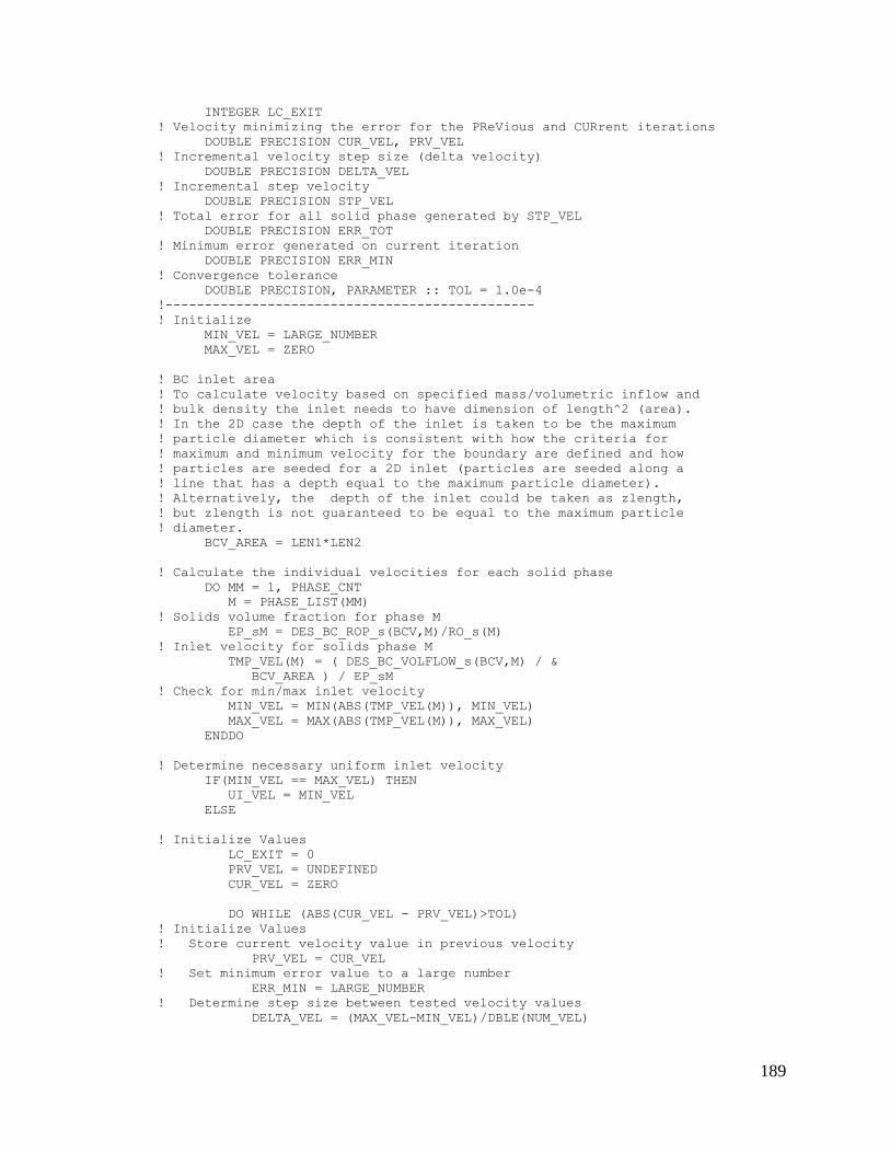
189

INTEGER LC_EXIT

! Velocity minimizing the error for the PReVious and CURrent iterations

DOUBLE PRECISION CUR_VEL, PRV_VEL

! Incremental velocity step size (delta velocity)

DOUBLE PRECISION DELTA_VEL

! Incremental step velocity

DOUBLE PRECISION STP_VEL

! Total error for all solid phase generated by STP_VEL

DOUBLE PRECISION ERR_TOT

! Minimum error generated on current iteration

DOUBLE PRECISION ERR_MIN

! Convergence tolerance

DOUBLE PRECISION, PARAMETER :: TOL = 1.0e-4

!-----------------------------------------------

! Initialize

MIN_VEL = LARGE_NUMBER

MAX_VEL = ZERO

! BC inlet area

! To calculate velocity based on specified mass/volumetric inflow and

! bulk density the inlet needs to have dimension of length^2 (area).

! In the 2D case the depth of the inlet is taken to be the maximum

! particle diameter which is consistent with how the criteria for

! maximum and minimum velocity for the boundary are defined and how

! particles are seeded for a 2D inlet (particles are seeded along a

! line that has a depth equal to the maximum particle diameter).

! Alternatively, the depth of the inlet could be taken as zlength,

! but zlength is not guaranteed to be equal to the maximum particle

! diameter.

BCV_AREA = LEN1*LEN2

! Calculate the individual velocities for each solid phase

DO MM = 1, PHASE_CNT

M = PHASE_LIST(MM)

! Solids volume fraction for phase M

EP_sM = DES_BC_ROP_s(BCV,M)/RO_s(M)

! Inlet velocity for solids phase M

TMP_VEL(M) = ( DES_BC_VOLFLOW_s(BCV,M) / &

BCV_AREA ) / EP_sM

! Check for min/max inlet velocity

MIN_VEL = MIN(ABS(TMP_VEL(M)), MIN_VEL)

MAX_VEL = MAX(ABS(TMP_VEL(M)), MAX_VEL)

ENDDO

! Determine necessary uniform inlet velocity

IF(MIN_VEL == MAX_VEL) THEN

UI_VEL = MIN_VEL

ELSE

! Initialize Values

LC_EXIT = 0

PRV_VEL = UNDEFINED

CUR_VEL = ZERO

DO WHILE (ABS(CUR_VEL - PRV_VEL)>TOL)

! Initialize Values

! Store current velocity value in previous velocity

PRV_VEL = CUR_VEL

! Set minimum error value to a large number

ERR_MIN = LARGE_NUMBER

! Determine step size between tested velocity values

DELTA_VEL = (MAX_VEL-MIN_VEL)/DBLE(NUM_VEL)

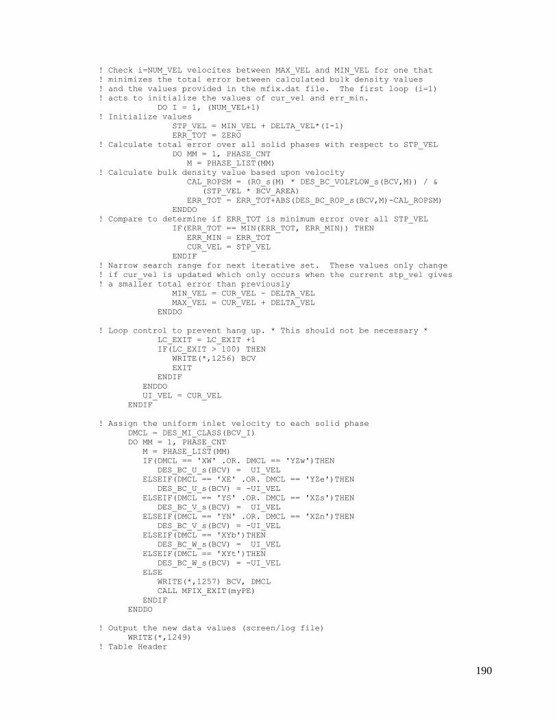
190

! Check i=NUM_VEL velocites between MAX_VEL and MIN_VEL for one that

! minimizes the total error between calculated bulk density values

! and the values provided in the mfix.dat file. The first loop (i=1)

! acts to initialize the values of cur_vel and err_min.

DO I = 1, (NUM_VEL+1)

! Initialize values

STP_VEL = MIN_VEL + DELTA_VEL*(I-1)

ERR_TOT = ZERO

! Calculate total error over all solid phases with respect to STP_VEL


M = PHASE_LIST(MM)

! Calculate bulk density value based upon velocity

CAL_ROPSM = (RO_s(M) * DES_BC_VOLFLOW_s(BCV,M)) / &

(STP_VEL * BCV_AREA)

ERR_TOT = ERR_TOT+ABS(DES_BC_ROP_s(BCV,M)-CAL_ROPSM)

ENDDO

! Compare to determine if ERR_TOT is minimum error over all STP_VEL

IF(ERR_TOT == MIN(ERR_TOT, ERR_MIN)) THEN

ERR_MIN = ERR_TOT

CUR_VEL = STP_VEL

ENDIF

! Narrow search range for next iterative set. These values only change

! if cur_vel is updated which only occurs when the current stp_vel gives

! a smaller total error than previously

MIN_VEL = CUR_VEL - DELTA_VEL

MAX_VEL = CUR_VEL + DELTA_VEL

ENDDO

! Loop control to prevent hang up. * This should not be necessary *

LC_EXIT = LC_EXIT +1

IF(LC_EXIT > 100) THEN

WRITE(*,1256) BCV

EXIT

ENDIF

ENDDO

UI_VEL = CUR_VEL

ENDIF

! Assign the uniform inlet velocity to each solid phase

DMCL = DES_MI_CLASS(BCV_I)


M = PHASE_LIST(MM)

IF(DMCL == 'XW' .OR. DMCL == 'YZw')THEN

DES_BC_U_s(BCV) = UI_VEL

ELSEIF(DMCL == 'XE' .OR. DMCL == 'YZe')THEN

DES_BC_U_s(BCV) = -UI_VEL

ELSEIF(DMCL == 'YS' .OR. DMCL == 'XZs')THEN

DES_BC_V_s(BCV) = UI_VEL

ELSEIF(DMCL == 'YN' .OR. DMCL == 'XZn')THEN

DES_BC_V_s(BCV) = -UI_VEL

ELSEIF(DMCL == 'XYb')THEN

DES_BC_W_s(BCV) = UI_VEL

ELSEIF(DMCL == 'XYt')THEN

DES_BC_W_s(BCV) = -UI_VEL

ELSE

WRITE(*,1257) BCV, DMCL


ENDIF

ENDDO

! Output the new data values (screen/log file)

WRITE(*,1249)

! Table Header

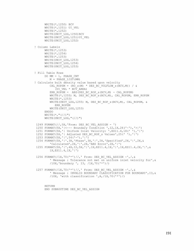
191

WRITE(*,1250) BCV

WRITE(*,1251) UI_VEL

WRITE(*,1252)


WRITE(UNIT_LOG,1251)UI_VEL

WRITE(UNIT_LOG,1252)

! Column Labels

WRITE(*,1253)

WRITE(*,1254)

WRITE(*,1253)




! Fill Table Rows


M = PHASE_LIST(MM)

! Calculate bulk density value based upon velocity

CAL_ROPSM = (RO_s(M) * DES_BC_VOLFLOW_s(BCV,M)) / &

(UI_VEL * BCV_AREA)

ERR_ROPSM = ABS(DES_BC_ROP_s(BCV,M) - CAL_ROPSM)

WRITE(*,1255) M, DES_BC_ROP_s(BCV,M), CAL_ROPSM, ERR_ROPSM

WRITE(*,1253)

WRITE(UNIT_LOG,1255) M, DES_BC_ROP_s(BCV,M), CAL_ROPSM, &

ERR_ROPSM


ENDDO

WRITE(*,"(//)")

WRITE(UNIT_LOG,"(//)")

1249 FORMAT(//,5X,'From: DES_BC_VEL_ASSIGN - ')

1250 FORMAT(5X,'|<--- Boundary Condition ',I2,1X,26('-'),'>|')

1251 FORMAT(5X,'| Uniform Inlet Velocity: ',ES11.4,18(' '),'|')

1252 FORMAT(5X,'| Adjusted DES_BC_ROP_s Values',25(' '),'|')

1253 FORMAT(5X,'|',54('-'),'|')

1254 FORMAT(5X,'|',3X,'Phase',3X,'|',2X,'Specified',2X,'|',2X,&

'Calculated',2X,'|',2X,'ABS Error',2X,'|')

1255 FORMAT(5X,'|',4X,I2,5X,'|',1X,ES11.4,1X,'|',1X,ES11.4,2X,'|',&

1X,ES11.4,1X,'|')

1256 FORMAT(/1X,70('*')//,' From: DES_BC_VEL_ASSIGN -',/,&

' Message : Tolerance not met on uniform inlet velocity for',&

/10X,'boundary ', I3, /1X,70('*')/)

1257 FORMAT(/1X,70('*')//,' From: DES_BC_VEL_ASSIGN -',/,&

' Message : INVALID BOUNDARY CLASSIFICATION FOR BOUNDARY',I3,&

/10X, 'with classification ',A,/1X,70('*')/)

RETURN

END SUBROUTINE DES_BC_VEL_ASSIGN

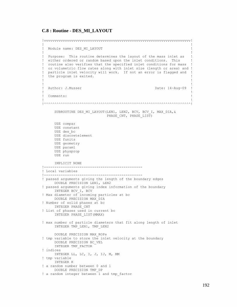
192

C.8 : Routine - DES_MI_LAYOUT


! !

! Module name: DES_MI_LAYOUT !

! !

! Purpose: This routine determines the layout of the mass inlet as !

! either ordered or random based upon the inlet conditions. This !

! routine also verifies that the specified inlet conditions for mass !

! or volumetric flow rates along with inlet size (length or area) and !

! particle inlet velocity will work. If not an error is flagged and !

! the program is exited. !

! !

! !


! !

! Comments: !

! !

!^^^^^^^^^^^^^^^^^^^^^^^^^^^^^^^^^^^^^^^^^^^^^^^^^^^^^^^^^^^^^^^^^^^^^^!

SUBROUTINE DES_MI_LAYOUT(LEN1, LEN2, BCV, BCV_I, MAX_DIA,&


USE compar

USE constant

USE des_bc

USE discretelement

USE funits

USE geometry

USE param1

USE physprop

USE run

IMPLICIT NONE

!-----------------------------------------------

! Local variables

!-----------------------------------------------

! passed arguments giving the length of the boundary edges

DOUBLE PRECISION LEN1, LEN2


INTEGER BCV_I, BCV




INTEGER PHASE_CNT



! max number of particle diameters that fit along length of inlet

INTEGER TMP_LEN1, TMP_LEN2

DOUBLE PRECISION MAX_ROPs

! tmp variable to store the inlet velocity at the boundary

DOUBLE PRECISION BC_VEL

INTEGER TMP_FACTOR

! indices

INTEGER LL, LC, I, J, IJ, M, MM

! tmp variable

INTEGER K

! a random number between 0 and 1

DOUBLE PRECISION TMP_DP

! a random integer between 1 and tmp_factor

193

INTEGER TMP_INT

! Temp variable for DES_MI_CLASS(BCV_I)

CHARACTER*3 DMCL

! lower threshold velocities that will work given the flow boundary

! specifications:

! lower maximum inlet particle velocity (MAXIPV); above which particles

! enter fast enough not to require additional handling

! lowest minimum inlet particle velocity (MINIPV) below which particles

! do not enter fast enough to meet the massflow rate and an error is

! flagged; above minipv and below maxipv the particle inlet conditions

! are adequate but must be carefully controlled

DOUBLE PRECISION MAXIPV, MINIPV

!-----------------------------------------------

IF(LEN2 == ZERO)THEN ! 2D domain

!-----------------------------------------------

TMP_LEN1 = FLOOR(real(LEN1/MAX_DIA))

TMP_LEN2 = ZERO

! notes :

! dtsolid*pi_factor(:) = time elapsed between particle injections

! = des_mi_time(:)

! d_p0/(dtsolid*pi_factor(:)) = approx velocity needed to move one particle

! diameter at the specified mass flow rate

! ceiling(tmp_len1/2) = the minimum no. of particles that can

! be arranged along the inlet so that an

! additional particle cannot fit

! k > 1 represents cases with more than 1 particles injected in a single

! solids timestep

K = PI_COUNT(BCV_I)

MAXIPV = MAX_DIA/( DTSOLID*dble(PI_FACTOR(BCV_I))*&

dble( FLOOR( CEILING( real(TMP_LEN1)/2.0 ) /real(K) ) ))

MINIPV = MAX_DIA/( DTSOLID*dble(PI_FACTOR(BCV_I))*&

dble( FLOOR( real(TMP_LEN1)/real(K) ) ))

IF (MINIPV .LT. SMALL_NUMBER) MINIPV = ZERO


! Check each solid phase to determine how the particles are to be

! placed and if the mass inflow conditions can be achevied.

IF(DMCL == 'XW' .OR. DMCL == "XE")THEN

BC_VEL = ABS(DES_BC_U_s(BCV))

ELSEIF(DMCL == 'YS' .OR. DMCL == "YN")THEN

BC_VEL = ABS(DES_BC_V_s(BCV))

ENDIF

! The bc velocity is lowered by a small number to prevent possible

! issues with the mantissa truncation

IF(MAXIPV .LE. (BC_VEL - SMALL_NUMBER))THEN

! The inlet velocity is sufficient to permit random placement of the new

! particles without risk of overlap

PARTICLE_PLCMNT(BCV_I) = 'RAND'

! Override the random placement for an ordered inlet

IF(FORCE_ORD_BC) PARTICLE_PLCMNT(BCV_I) = 'ORDR'

ELSEIF(MINIPV .LE. (BC_VEL - SMALL_NUMBER) .AND. &

(BC_VEL .LT. MAXIPV + SMALL_NUMBER)) THEN

! Then inlet velocity will require that the new particles be placed with

! order to prevent overlap.

PARTICLE_PLCMNT(BCV_I) = 'ORDR'

ELSE

! The inlet velocity is too low to satisfy the other inlet conditions.

194

! Determine maximum possible ROP_s values that will satisfy the inlet

! conditions. Flag error, prompt with new values, and exit.

WRITE(UNIT_LOG,1300) BCV

WRITE(*,1300) BCV


M = PHASE_LIST(MM)

! Even though the system is 2D, an area of the inlet is needed for

! the following calculation. This 'depth' is taken as max_dia.

MAX_ROPs = (DES_BC_VOLFLOW_s(BCV,M)*RO_s(M)) / &

(MINIPV * LEN1 * MAX_DIA)

WRITE(UNIT_LOG,1301) BCV, M, MAX_ROPs

WRITE(*,1301) BCV, M, MAX_ROPs

ENDDO


WRITE(*,1302)


ENDIF

IF(PARTICLE_PLCMNT(BCV_I) == 'ORDR')THEN

! In 2D calculate the approx. particle line density (e.g., the no. of

! particles along the inlet) needed to achieve the specified particle

! mass flow rate and particle velocity;

TMP_FACTOR = CEILING(real(MAX_DIA / &

(dble(PI_FACTOR(BCV_I)) * DTSOLID * ABS(BC_VEL))))

ALLOCATE( MI_ORDER(BCV_I)%VALUE( TMP_FACTOR ) )

ALLOCATE( I_OF_MI(BCV_I)%VALUE( TMP_FACTOR ) )

! Initialize

MI_ORDER(BCV_I)%VALUE(:) = -1

MI_FACTOR(BCV_I) = 1

! Dimension of grid cell; this may be larger than than the particle

! diameter but not smaller

MI_WINDOW(BCV_I) = LEN1/dble(TMP_FACTOR)

DO I = 1, TMP_FACTOR

I_OF_MI(BCV_I)%VALUE(I) = I - 1

ENDDO

! Construct an array of integers from 1 to TMP_FACTOR in a random

! order. This is used when placing new particles.

LL = 1

DO WHILE (MI_ORDER(BCV_I)%VALUE(TMP_FACTOR) .EQ. -1)

CALL RANDOM_NUMBER(TMP_DP)

TMP_INT = CEILING(real(TMP_DP*dble(TMP_FACTOR)))

DO LC = 1, LL

IF(TMP_INT .EQ. MI_ORDER(BCV_I)%VALUE(LC) )EXIT

IF(LC .EQ. LL)THEN

MI_ORDER(BCV_I)%VALUE(LC) = TMP_INT

LL = LL + 1

ENDIF

ENDDO

ENDDO

ENDIF ! endif particle_plcmnt(bcv_i) == 'ordr'

ELSEIF(LEN2 /= ZERO) THEN ! 3D domain

!-----------------------------------------------



K = PI_COUNT(BCV_I)

! In the 3D case the calculation for MAXIPV is conservative. That is,

! the actual bc velocity could be somewhat lower than the calculated

! value of MAXIPV and still allow for random particle placement

195

MAXIPV = MAX_DIA/( DTSOLID*dble(PI_FACTOR(BCV_I)) * &

dble( FLOOR( CEILING( &

real(TMP_LEN1*TMP_LEN2)/2.0 ) /real(K) ) ))

! The cutoff is associated with square packing of disks on a plane

! A lower velocity would be possible with hexagonal packing

MINIPV = MAX_DIA/( DTSOLID*dble(PI_FACTOR(BCV_I)) * &

dble( FLOOR( real(TMP_LEN1*TMP_LEN2)/real(K) ) ))

IF (MINIPV .LT. SMALL_NUMBER) MINIPV = ZERO


! Check each solid phase to determine how the particles are to be

! placed or if the mass inflow conditions can be achevied.

IF(DMCL == 'YZe' .OR. DMCL == "YZw")THEN

BC_VEL = ABS(DES_BC_U_s(BCV))

ELSEIF(DMCL == 'XZs' .OR. DMCL == "XZn")THEN

BC_VEL = ABS(DES_BC_V_s(BCV))

ELSEIF(DMCL == 'XYb' .OR. DMCL == "XYt")THEN

BC_VEL = ABS(DES_BC_W_s(BCV))

ENDIF

! The bc velocity is lowered by a small number to prevent possible

! issues with the mantissa truncation

IF(MAXIPV .LE. (ABS(BC_VEL) - SMALL_NUMBER))THEN

! The inlet velocity is sufficient to permit random placement of the new

! particles without risk of overlap

PARTICLE_PLCMNT(BCV_I) = 'RAND'

! Override the random placement for an ordered inlet

IF(FORCE_ORD_BC) PARTICLE_PLCMNT(BCV_I) = 'ORDR'

ELSEIF(MINIPV .LE. (BC_VEL - SMALL_NUMBER) .AND. &

(BC_VEL .LT. MAXIPV + SMALL_NUMBER)) THEN

! Then inlet velocity will require that the new particles be placed with

! order to prevent overlap.

PARTICLE_PLCMNT(BCV_I) = 'ORDR'

ELSE

! The inlet velocity is too low to satisfy the other inlet conditions.

! Determine maximum possible ROP_s values that will satisfy the inlet

! conditions. Flag error, propt with new values, and exit.

WRITE(UNIT_LOG,1300)BCV; WRITE(*,1300)BCV


M = PHASE_LIST(MM)

MAX_ROPs = (DES_BC_VOLFLOW_s(BCV,M)*RO_s(M)) / &

(MINIPV * LEN1 * LEN2)

WRITE(UNIT_LOG,1301)BCV,M,MAX_ROPs

WRITE(*,1301)BCV,M,MAX_ROPs

ENDDO


WRITE(*,1302)


ENDIF


! In 3D calculate the the number of grid cells within the inlet face

! with length dimension of 1 particle diameter

TMP_FACTOR = TMP_LEN1 * TMP_LEN2

ALLOCATE( MI_ORDER(BCV_I)%VALUE( TMP_FACTOR ) )

ALLOCATE( I_OF_MI(BCV_I)%VALUE( TMP_FACTOR ) )

ALLOCATE( J_OF_MI(BCV_I)%VALUE( TMP_FACTOR ) )

! Initialize

MI_ORDER(BCV_I)%VALUE(:) = -1


! Dimension of grid cell; this may be larger than than the particle

! diameter but not smaller:

196

! if len1/tmp_len1 < len2/tmp_len2, len1/tmp_len1*tmp_len2 < len2 or

! if len1/tmp_len1 > len2/tmp_len2, len2/tmp_len2*tmp_len1 < len1

MI_WINDOW(BCV_I) = MIN(LEN1/TMP_LEN1, LEN2/TMP_LEN2)

DO I = 1, TMP_LEN1

DO J = 1, TMP_LEN2

IJ = J + (I-1)*TMP_LEN2

I_OF_MI(BCV_I)%VALUE(IJ) = I - 1

J_OF_MI(BCV_I)%VALUE(IJ) = J - 1

ENDDO

ENDDO

! Construct an array of integers from 1 to TMP_FACTOR in a random

! order. This is used when placing new particles.

LL = 1

DO WHILE (MI_ORDER(BCV_I)%VALUE(TMP_FACTOR) .EQ. -1)

CALL RANDOM_NUMBER(TMP_DP)

TMP_INT = CEILING(real(TMP_DP*dble(TMP_FACTOR)))

DO LC = 1, LL

IF(TMP_INT .EQ. MI_ORDER(BCV_I)%VALUE(LC) )EXIT

IF(LC .EQ. LL)THEN

MI_ORDER(BCV_I)%VALUE(LC) = TMP_INT

LL = LL + 1

ENDIF

ENDDO

ENDDO

ENDIF ! endif particle_plcmnt(bcv_i) == 'ordr'

ENDIF ! endif len2 == zero

WRITE(*,1303) BCV, LEN1, LEN2, TMP_LEN1, TMP_LEN2,&

MAXIPV, MINIPV, PARTICLE_PLCMNT(BCV_I)

1300 FORMAT(/1X,70('*')//,' From: DES_MI_LAYOUT -',/,&

' Message: DES_BC_ROP_s values for BC ',I3,' are set too ',&

'high.',/,10X,'The MAXIMUM values for the supplied inlet ',&

'conditions are:')

1301 FORMAT(10X,'DES_BC_ROP_s(',I3,',',I3,') < ',F9.4)

1302 FORMAT(1X,70('*'))

1303 FORMAT(5X,'From: DES_MI_LAYOUT - BC: ', I3, /7X,&

'LEN1 = ', ES17.5,4X, ' LEN2 = ', ES17.5,/7X,&

'TMP_LEN1 = ', I6,11X, ' TMP_LEN2 = ', I6,/7X,&

'MAXIPV = ', ES17.5,2X,' MINIPV = ', ES17.5,/7X,&

'PLCMNT = ',3X,A,//)

RETURN

END SUBROUTINE DES_MI_LAYOUT

197

C.9 : Routine - DES_MI_CELS


! !

! Module name: DES_MI_CELLS !

! !

! Purpose: !

! Locate the i, j, k position of the cells encompassing the DES

! mass inlet BC so that when particles are injected into the system,

! a complete grid search is not necessary to prevent/determine:

! 1) the injected particle from overlapping with an existing

! particle nearby when particle_plcmnt = 'rand'

! 2) the i, j, k indices of the newly injected particle on the

! eulerian grid defined by imax, jmax, kmax

! !

! Author: J.Musser Date: 5-Oct-09 !

! !

! Comments: !

! !

!^^^^^^^^^^^^^^^^^^^^^^^^^^^^^^^^^^^^^^^^^^^^^^^^^^^^^^^^^^^^^^^^^^^^^^!

SUBROUTINE DES_MI_CELLS(BCV, BCV_I)

USE des_bc

USE discretelement

USE geometry

IMPLICIT NONE

!-----------------------------------------------

! Local variables

!-----------------------------------------------


INTEGER BCV_I, BCV

INTEGER I,J,K

! dummy variable for length calculations

DOUBLE PRECISION LOCATION

!-----------------------------------------------


IF(DES_BC_X_w(BCV) == ZERO) GS_ARRAY(BCV_I,1:2) = 1

IF(DES_BC_X_w(BCV) == XLENGTH) GS_ARRAY(BCV_I,1:2) = IMAX2

ELSE

! note dx(1) = length of ghost cell (x < zero)

I=2; LOCATION = ZERO

DO WHILE (LOCATION <= XLENGTH)

IF((DES_BC_X_w(BCV) >= LOCATION) .AND. &

(DES_BC_X_w(BCV) < LOCATION + DX(I))) THEN

GS_ARRAY(BCV_I,1) = I

ENDIF

IF((DES_BC_X_e(BCV) >= LOCATION) .AND. &

(DES_BC_X_e(BCV) < LOCATION + DX(I))) THEN

GS_ARRAY(BCV_I,2) = I

EXIT

ENDIF

LOCATION = LOCATION + DX(I)

I=I+1

ENDDO

ENDIF


198

IF(DES_BC_Y_s(BCV) == ZERO) GS_ARRAY(BCV_I,3:4) = 1

IF(DES_BC_Y_s(BCV) == YLENGTH) GS_ARRAY(BCV_I,3:4) = JMAX2

ELSE

! note dy(1) = length of ghost cell (y < zero)

J=2; LOCATION = ZERO

DO WHILE (LOCATION <= YLENGTH)

IF((DES_BC_Y_s(BCV) >= LOCATION) .AND. &

(DES_BC_Y_s(BCV) < LOCATION + DY(J))) THEN

GS_ARRAY(BCV_I,3) = J

ENDIF

IF((DES_BC_Y_n(BCV) >= LOCATION) .AND. &

(DES_BC_Y_n(BCV) < LOCATION + DY(J))) THEN

GS_ARRAY(BCV_I,4) = J

EXIT

ENDIF

LOCATION = LOCATION + DY(J)

J=J+1

ENDDO

ENDIF

IF(DIMN == 2) THEN

GS_ARRAY(BCV_I,5:6) = 1

ELSE


IF(DES_BC_Z_b(BCV) == ZERO) GS_ARRAY(BCV_I,5:6) = 1

IF(DES_BC_Z_b(BCV) == ZLENGTH) GS_ARRAY(BCV_I,5:6) = KMAX2

ELSE

K=2; LOCATION = ZERO

DO WHILE (LOCATION <= ZLENGTH)

IF((DES_BC_Z_b(BCV) >= LOCATION) .AND. &

(DES_BC_Z_b(BCV) < LOCATION + DZ(K))) THEN

GS_ARRAY(BCV_I,5) = K

ENDIF

IF((DES_BC_Z_t(BCV) >= LOCATION) .AND. &

(DES_BC_Z_t(BCV) < LOCATION + DZ(K))) THEN

GS_ARRAY(BCV_I,6) = K

EXIT

ENDIF

LOCATION = LOCATION + DZ(K)

K=K+1

ENDDO

ENDIF

ENDIF

RETURN

END SUBROUTINE DES_MI_CELLS

199

C.10 : Routine - DES_MO_CLASSIFY


! !

! Module name: DES_MO_CLASSIFY !

! !

! Purpose: !

! !


! !

! Comments: !

! !

!^^^^^^^^^^^^^^^^^^^^^^^^^^^^^^^^^^^^^^^^^^^^^^^^^^^^^^^^^^^^^^^^^^^^^^!

SUBROUTINE DES_MO_CLASSIFY(BCV_I, BCV)

USE compar

USE constant

USE des_bc

USE discretelement

USE funits

USE geometry

USE param1

USE physprop

USE run

IMPLICIT NONE

!-----------------------------------------------

! Local variables

!-----------------------------------------------


INTEGER BCV_I, BCV

!-----------------------------------------------


! Check verticle mass outlet: 2D

! ----------------------------------------


DES_MO_X = .TRUE.

IF (DES_BC_X_w(BCV) == ZERO) DES_MO_CLASS(BCV_I) = 'XW'

IF (DES_BC_X_w(BCV) == XLENGTH) DES_MO_CLASS(BCV_I) = 'XE'

ENDIF

! Check horizontal mass outlet: 2D

! ----------------------------------------


DES_MO_Y = .TRUE.

IF (DES_BC_Y_s(BCV) == ZERO) DES_MO_CLASS(BCV_I) = 'YS'

IF (DES_BC_Y_s(BCV) == YLENGTH) DES_MO_CLASS(BCV_I) = 'YN'

ENDIF

ELSE ! 3D domain

! Check mass outlet on YZ face: 3D

! ----------------------------------------

! see comments following the yz face section of des_mi_classify

! for elucidation on this, and subsequent series of if statements



200


.OR. &




DES_BC_Y_s(BCV) /= YLENGTH &

.OR. &





DES_MO_X = .TRUE.

IF (DES_BC_X_w(BCV) == ZERO) DES_MO_CLASS(BCV_I) = 'XW'

IF (DES_BC_X_w(BCV) == XLENGTH) DES_MO_CLASS(BCV_I) = 'XE'

ENDIF

! End check mass outlet on YZ face: 3D

! Check mass inlet on XZ face: 3D

! ----------------------------------------

IF(DES_BC_Y_s(BCV) == DES_BC_Y_n(BCV) .AND. &



.OR. &





.OR. &





DES_MO_Y = .TRUE.

IF (DES_BC_Y_s(BCV) == ZERO) DES_MO_CLASS(BCV_I) = 'YS'

IF (DES_BC_Y_s(BCV) == YLENGTH) DES_MO_CLASS(BCV_I) = 'YN'

ENDIF

! End check mass outlet on XZ face: 3D

! Check mass inlet on XY face: 3D

! ----------------------------------------

IF(DES_BC_Z_b(BCV) == DES_BC_Z_t(BCV) .AND. &


DES_BC_Y_s(BCV) /= DES_BC_Y_n(BCV) &

.OR. &





.OR. &





DES_MO_Z = .TRUE.

IF (DES_BC_Z_b(BCV) == ZERO) DES_MO_CLASS(BCV_I) = 'ZB'

IF (DES_BC_Z_b(BCV) == ZLENGTH) DES_MO_CLASS(BCV_I) = 'ZT'

201

ENDIF

! End check mass outlet on XY face: 3D

ENDIF ! endif dimn == 2

! Verify that an inlet is not on a face that is connected to a periodic

! boundary condition. If so, write error message and exit.

! No Xew outlet with X direction periodic walls

IF((DES_MO_CLASS(BCV_I) == 'XW' .OR. DES_MO_CLASS(BCV_I) == 'XE') &

.AND. DES_PERIODIC_WALLS_X) THEN

WRITE (UNIT_LOG, 1500) BCV, 'DES_PERIODIC_WALLS_X'

WRITE (*, 1500) BCV, 'DES_PERIODIC_WALLS_X'


ENDIF

! No Ysn outlet with Y direction periodic walls

IF((DES_MO_CLASS(BCV_I) == 'YS' .OR. DES_MO_CLASS(BCV_I) == 'YN') &

.AND. DES_PERIODIC_WALLS_Y) THEN

WRITE (UNIT_LOG, 1500) BCV, 'DES_PERIODIC_WALLS_Y'

WRITE (*, 1500) BCV, 'DES_PERIODIC_WALLS_Y'


ENDIF

! No Zbt outlet with Z direction periodic walls

IF((DES_MO_CLASS(BCV_I) == 'ZB' .OR. DES_MO_CLASS(BCV_I) == 'ZT') &

.AND. DES_PERIODIC_WALLS_Z) THEN

WRITE (UNIT_LOG, 1500) BCV, 'DES_PERIODIC_WALLS_Z'

WRITE (*, 1500) BCV, 'DES_PERIODIC_WALLS_Z'


ENDIF

1500 FORMAT(/1X,70('*')//,' From: DES_MI_CLASSIFY -',/10X,&

'DEM outlets can not be placed on a periodic boundary.',/10X,&

'Check DEM boundary condtion ',I2,' and ',A,'.',/1X,70('*')/)

RETURN

END SUBROUTINE DES_MO_CLASSIFY

202

C.11 : Routine - DES_MIO_PERIODIC


! !

! Module name: DES_MIO_PERIODIC !

! !

! Purpose: ! Verify that any inlet or outlet is placed at least !

! "SPACER" distace away from a periodic boundary condition. This !

! will prevent any particle that crossing a periodic boundary from !

! being moved into contact with an entering or exiting particle. !

! This is necessary since particles are not incrementally moved !

! across a periodic boundary. !

! !

! Author: J.Musser Date: 22-Dec-09 !

! !

! Comments: !

! !

!^^^^^^^^^^^^^^^^^^^^^^^^^^^^^^^^^^^^^^^^^^^^^^^^^^^^^^^^^^^^^^^^^^^^^^!

SUBROUTINE DES_MIO_PERIODIC(BCV,BCV_I,CLASS, MAX_DIA)

USE compar

USE des_bc

USE discretelement

USE funits

USE geometry

USE physprop

IMPLICIT NONE

!-----------------------------------------------

! Local variables

!-----------------------------------------------

! boundary classification of inlet or outlet (MI or MO)

CHARACTER*2 CLASS

! boundary classification of inlet or outlet (full text for messages)

CHARACTER*6 IO_ID

! value of DES_MI/MO_CLASS (boundary plane that MI or MO is

! located on)

CHARACTER*3 DMC

INTEGER BCV ! absolute boundary condition number

INTEGER BCV_I ! index boundary condtion number



! buffer space around inlets and outlets with boardering periodic

! boundary conditions

DOUBLE PRECISION SPACER

!-----------------------------------------------

SPACER = 1.05d0 * MAX_DIA

IF(CLASS == 'MI')THEN

DMC = DES_MI_CLASS(BCV_I)

IO_ID = "inlet"

ELSE

203

DMC = DES_MO_CLASS(BCV_I)

IO_ID = "outlet"

ENDIF

IF(DMC == 'XW' .OR. DMC == 'XE' .OR. & ! 2D inlet \ 2D-3D outlet

DMC == 'YZw' .OR. DMC == 'YZe') THEN ! 3D inlet

IF(DES_PERIODIC_WALLS_Y) THEN

IF(DES_BC_Y_s(BCV) < SPACER .OR. &

DES_BC_Y_n(BCV) > (YLENGTH - SPACER)) THEN

WRITE(UNIT_LOG, 1600) IO_ID, BCV, 'Y'

WRITE(*, 1600) IO_ID, BCV, 'Y'


ENDIF

ENDIF

IF(DES_PERIODIC_WALLS_Z) THEN

IF(DES_BC_Z_b(BCV) < SPACER .OR. &

DES_BC_Z_t(BCV) > (ZLENGTH - SPACER)) THEN

WRITE(UNIT_LOG, 1600) IO_ID, BCV, 'Z'

WRITE(*, 1600) IO_ID, BCV, 'Z'


ENDIF

ENDIF

ENDIF

IF(DMC == 'YS' .OR. DMC == 'YN' .OR. & ! 2D inlet \ 2D-3D outlet

DMC == 'XZs' .OR. DMC == 'XZn') THEN ! 3D inlet

IF(DES_PERIODIC_WALLS_X) THEN

IF(DES_BC_X_w(BCV) < SPACER .OR. &

DES_BC_X_e(BCV) > (XLENGTH - SPACER)) THEN

WRITE(UNIT_LOG, 1600) IO_ID, BCV, 'X'

WRITE(*, 1600) IO_ID, BCV, 'X'


ENDIF

ENDIF

IF(DES_PERIODIC_WALLS_Z) THEN

IF(DES_BC_Z_b(BCV) < SPACER .OR. &

DES_BC_Z_t(BCV) > (ZLENGTH - SPACER)) THEN

WRITE(UNIT_LOG, 1600) IO_ID, BCV, 'Z'

WRITE(*, 1600) IO_ID, BCV, 'Z'


ENDIF

ENDIF

ENDIF

IF(DMC == 'XYb' .OR. DMC == 'XYt' .OR. & ! 3D inlet

DMC == 'ZB' .OR. DMC == 'ZT') THEN ! 3D outlet

IF(DES_PERIODIC_WALLS_X) THEN

IF(DES_BC_X_w(BCV) < SPACER .OR. &

DES_BC_X_e(BCV) > (XLENGTH - SPACER)) THEN

WRITE(UNIT_LOG, 1600) IO_ID, BCV, 'X'

WRITE(*, 1600) IO_ID, BCV, 'X'


ENDIF

ENDIF

IF(DES_PERIODIC_WALLS_Y) THEN

IF(DES_BC_Y_s(BCV) < SPACER .OR. &

DES_BC_Y_n(BCV) > (YLENGTH - SPACER)) THEN

WRITE(UNIT_LOG, 1600) IO_ID, BCV, 'Y'

WRITE(*, 1600) IO_ID, BCV, 'Y'


ENDIF

ENDIF

204

ENDIF

1600 FORMAT(/1X,70('*')//, ' From: CHECK_DES_BC -',/,&

' Message: DES ',A,' boundary ',I3,' is too close to',&

' DES_PERIODIC_WALLS_',A,'.',/1X,70('*')/)

RETURN

END SUBROUTINE DES_MIO_PERIODIC

205

C.12 : Routine - DES_MASS_INLET


! !

! Module name: DES_MASS_INLET(BCV_I) !

! !

! Purpose: This routine fills in the necessary information for new !

! particles entereing the system. !

! !

! !


! !

! Comments: !

! !

!^^^^^^^^^^^^^^^^^^^^^^^^^^^^^^^^^^^^^^^^^^^^^^^^^^^^^^^^^^^^^^^^^^^^^^!

SUBROUTINE DES_MASS_INLET(BCV_I)

USE compar

USE constant

USE des_bc

USE discretelement

USE funits

USE geometry

USE indices

USE param1

USE physprop

IMPLICIT NONE

!-----------------------------------------------

! Local variables

!-----------------------------------------------

INTEGER IJK ! Necessary for function.inc

INTEGER I, J, K ! Indices

INTEGER IP, LL ! Loop indices

INTEGER LS ! Loop counter start value

INTEGER TMPI ! Loop counter

INTEGER NPG ! Number of particles in cell

INTEGER NP ! Particle id. number

INTEGER BCV_I, BCV ! Boundary Condition ID

INTEGER M ! Mass phase of new particle

! this variable temporarily stores the number ids of all particles

! in the ijk location of interest

INTEGER, DIMENSION(:), ALLOCATABLE :: HOLDER

! a random number between 0 and 1

DOUBLE PRECISION RAND

! random integer number between 1 and NUMFRAC_LIMIT

INTEGER RAND_I

! particle x,y,z position

DOUBLE PRECISION XPOS, YPOS, ZPOS

! size of mesh for grid based search

DOUBLE PRECISION SIZEDX, SIZEDY, SIZEDZ

!-----------------------------------------------

INCLUDE 'function.inc'

LS = 1

BCV = DES_BC_MI_ID(BCV_I)

DO IP = 1, PI_COUNT(BCV_I) !Loop over the particles being injected

206

! Check to see if MAX_PIS has been exceeded, if so, STOP

IF(PIS .GE. MAX_PIS) THEN


WRITE(*,1000)


ENDIF

! Find the first free space in the particle existance array

DO NP = LS, MAX_PIS

IF(.NOT.PEA(NP,1)) THEN

LS = NP

EXIT

ENDIF

ENDDO

! Set the flag in the particle existance array

PEA(NP,1) = .TRUE.

! Set the flag that the particle is new. This allows it to be ignored

! by various subroutines

PEA(NP,2) = .TRUE.

! Increment the particle in system value by one

PIS = PIS + 1

! Obtain a mass phase to assign to the incoming particle

IF(DES_BC_POLY(BCV_I)) THEN

CALL RANDOM_NUMBER(RAND)

! Scale and convert random number to an interger

RAND_I = CEILING(dble(NUMFRAC_LIMIT)*RAND)

M = DES_BC_POLY_LAYOUT(BCV_I,RAND_I)

ELSE

M = DES_BC_POLY_LAYOUT(BCV_I,1)

ENDIF

! Set the initial velocity values

DES_VEL_OLD(NP,1) = DES_BC_U_s(BCV)

DES_VEL_OLD(NP,2) = DES_BC_V_s(BCV)

IF(DIMN == 3) DES_VEL_OLD(NP,3) = DES_BC_W_s(BCV)

DES_VEL_NEW(NP,:) = DES_VEL_OLD(NP,:)

! Set the initial angular velocity values

OMEGA_OLD(NP,:) = 0

OMEGA_NEW(NP,:) = 0

! Set the particle radius value

DES_RADIUS(NP) = (D_P0(M) * HALF)

! Set the particle density value

RO_Sol(NP) = RO_S(M)

! Set the particle mass phase

PIJK(NP,5) = M

! Calculate the new particle's Volume, Mass, OMOI

PVOL(NP) = (4.0d0/3.0d0) * PI * DES_RADIUS(NP)**3

PMASS(NP) = PVOL(NP) * RO_Sol(NP)

OMOI(NP) = 5.d0 / (2.d0 * PMASS(NP) * DES_RADIUS(NP)**2)

! Set the initial position values based on mass inlet class

CALL DES_PLACE_NEW_PARTICLE(NP, BCV_I)

207

DES_POS_NEW(NP,:) = DES_POS_OLD(NP,:)

XPOS = DES_POS_NEW(NP,1)

YPOS = DES_POS_NEW(NP,2)

IF (DIMN == 3) THEN

ZPOS = DES_POS_NEW(NP,3)

ENDIF

! Determine the i, j, k indices of the cell containing the new

! particle(s) by checking the cells near the mass inlet using

! GS_ARRAY. Note the indices will place the particle in a ghost

! cell.

! ------------------------------------------------------------

DO I = GS_ARRAY(BCV_I,1), GS_ARRAY(BCV_I,2)

IF(XPOS < XE(1))THEN

PIJK(NP,1) = 1

EXIT

ELSEIF(XPOS >= XE(IMAX1))THEN

PIJK(NP,1) = IMAX2

EXIT

ELSEIF((XPOS >= XE(I-1)) .AND. (XPOS < XE(I))) THEN

PIJK(NP,1) = I

EXIT

ENDIF

ENDDO

DO J = GS_ARRAY(BCV_I,3), GS_ARRAY(BCV_I,4)

IF(YPOS < YN(1))THEN

PIJK(NP,2) = 1

EXIT

ELSEIF(YPOS >= YN(JMAX1))THEN

PIJK(NP,2) = JMAX2

EXIT

ELSEIF((YPOS >= YN(J-1)) .AND. (YPOS < YN(J))) THEN

PIJK(NP,2) = J

EXIT

ENDIF

ENDDO

IF(DIMN == 2) THEN

PIJK(NP,3) = 1

ELSE

DO K = GS_ARRAY(BCV_I,5), GS_ARRAY(BCV_I,6)

IF(ZPOS < ZT(1))THEN

PIJK(NP,3) = 1

EXIT

ELSEIF(ZPOS >= ZT(KMAX1))THEN

PIJK(NP,3) = KMAX2

EXIT

ELSEIF((ZPOS >= ZT(K-1)) .AND. (ZPOS < ZT(K))) THEN

PIJK(NP,3) = K

EXIT

ENDIF

ENDDO

ENDIF

! Update the PIC array for new particles so that any subsequent

! particles that are to be injected will be checked to prevent

! overlap with previously injected particles

I = PIJK(NP,1)

J = PIJK(NP,2)

K = PIJK(NP,3)

IJK = FUNIJK(I,J,K)

208

PIJK(NP,4) = IJK

IF (ASSOCIATED(PIC(I,J,K)%P)) THEN

NPG = SIZE(PIC(I,J,K)%P)

ALLOCATE( HOLDER (NPG) )

! store the particle no. id of all particles at the ijk location

TMPI = 1

DO LL = 1, NPG

HOLDER(TMPI) = PIC(I,J,K)%P(LL)

TMPI = TMPI + 1

ENDDO

DEALLOCATE(PIC(I,J,K)%P)

! essentially increasing the no. of particles at the ijk location by 1

ALLOCATE(PIC(I,J,K)%P(TMPI))

DO LL = 1, TMPI - 1

PIC(I,J,K)%P(LL) = HOLDER(LL)

ENDDO

! storing the new particle no. id in the list

PIC(I,J,K)%P(TMPI) = NP

DEALLOCATE(HOLDER)

ELSE

! no other particles were at this ijk location

TMPI = 1

ALLOCATE(PIC(I,J,K)%P(TMPI))

PIC(I,J,K)%P(TMPI) = NP

ENDIF

PINC(IJK) = TMPI

! If using des_neighbor_search option 4 (cell/grid based search) then

! determine the i,j,k indices of the cell containing the new particle

! based on the mesh for the grid based search. If cell is outside the

! domain then either set the index to 1 or add 2 to the index to

! account for ghost cells.

! Note that this section is probably unnecessary since the routine

! particles_in_cell will pickup the same information before neighbor

! search is ever called and it is only in the neighbor search routine

! that this information should be needed

! ------------------------------------------------------------

IF (DES_NEIGHBOR_SEARCH .EQ. 4) THEN

! determine size of the mesh

SIZEDX = XLENGTH/DESGRIDSEARCH_IMAX

SIZEDY = YLENGTH/DESGRIDSEARCH_JMAX

IF (DIMN .EQ. 2) THEN

SIZEDZ = ONE

ELSE

SIZEDZ = ZLENGTH/DESGRIDSEARCH_KMAX

ENDIF

IF (XPOS < 0) THEN

I = 1

ELSEIF (XPOS >= XLENGTH) THEN

I = DESGS_IMAX2

ELSE

I = INT(XPOS/SIZEDX)+2

ENDIF

IF (YPOS < 0 ) THEN

J = 1

ELSEIF (YPOS >= YLENGTH) THEN

J = DESGS_JMAX2

209

ELSE

J = INT(YPOS/SIZEDY)+2

ENDIF


K = 1

ELSE

IF (ZPOS < 0 ) THEN

K = 1

ELSEIF (ZPOS >= ZLENGTH) THEN

K = DESGS_KMAX2

ELSE

K = INT(ZPOS/SIZEDZ)+2

ENDIF

ENDIF

DESGRIDSEARCH_PIJK(NP,1) = I

DESGRIDSEARCH_PIJK(NP,2) = J

DESGRIDSEARCH_PIJK(NP,3) = K

! Update the DESGRIDSEARCH_PIC array for new particles. Note that

! is not needed to prevent subsequent particles that are injected

! from overlapping with previous particles as the variable PIC is

! used for that.

IF (ASSOCIATED(DESGRIDSEARCH_PIC(I,J,K)%P)) THEN

NPG = SIZE(DESGRIDSEARCH_PIC(I,J,K)%P)

ALLOCATE( HOLDER (NPG) )

! store the particle no. id of all particles at the ijk location

TMPI = 1

DO LL = 1, NPG

HOLDER(TMPI) = DESGRIDSEARCH_PIC(I,J,K)%P(LL)

TMPI = TMPI + 1

ENDDO

DEALLOCATE(DESGRIDSEARCH_PIC(I,J,K)%P)

! essentially increasing the no. of particles at the ijk location by 1

ALLOCATE(DESGRIDSEARCH_PIC(I,J,K)%P(TMPI))

DO LL = 1, TMPI - 1

DESGRIDSEARCH_PIC(I,J,K)%P(LL) = HOLDER(LL)

ENDDO

! storing the new particle no. id in the list

DESGRIDSEARCH_PIC(I,J,K)%P(TMPI) = NP

DEALLOCATE(HOLDER)

ELSE

! no other particles were at this ijk location

TMPI = 1

ALLOCATE(DESGRIDSEARCH_PIC(I,J,K)%P(TMPI))

DESGRIDSEARCH_PIC(I,J,K)%P(TMPI) = NP

ENDIF

ENDIF ! end if des_neighbor_search = 4

ENDDO ! end loop over the no. of injected particles (NP)

1000 FORMAT(/1X,70('*')//,' From: DES_MASS_INLET -',/&

' Message: Maximum number of particles in the system MAX_PIS',&

/10X,' has been exceeded. Increase the value in mfix.dat',/&

1X,70('*')/)

RETURN

END SUBROUTINE DES_MASS_INLET

210

C.13 : Routine - DES_PLACE_NEW_PARTICLE


! !

! Module name: DES_PLACE_NEW_PARTICLE !

! !

! Purpose: This routine uses the classification information to place !

! a new particle in the proper location. !

! !


! !

! Comments: !

! !

!^^^^^^^^^^^^^^^^^^^^^^^^^^^^^^^^^^^^^^^^^^^^^^^^^^^^^^^^^^^^^^^^^^^^^^!

SUBROUTINE DES_PLACE_NEW_PARTICLE(NP, BCV_I)

USE compar

USE des_bc

USE discretelement

USE funits

USE geometry

USE param1

USE physprop

IMPLICIT NONE

!-----------------------------------------------

! Local variables

!-----------------------------------------------

! the current particle no.

INTEGER NP

! the associated bc no.

INTEGER BCV_I, BCV

! a random number between 0-1

DOUBLE PRECISION RAND1, RAND2

! 'lower' x,y,z location of current window

DOUBLE PRECISION MI_WIN

! a random index number for I_OF_MI or J_OF_MI

INTEGER MI_ORD

!

LOGICAL TOUCHING

!-----------------------------------------------

TOUCHING = .TRUE.

BCV = DES_BC_MI_ID(BCV_I)

SELECT CASE(DES_MI_CLASS(BCV_I))

! 2D domain with verticle mass inlet: (west face)

! ----------------------------------------

CASE ('XW')

! Offset Y axis by 1 particle diameter (max diameter) into ghost cell

DES_POS_OLD(NP,1) = -(DES_BC_OFFSET(BCV_I))

IF(PARTICLE_PLCMNT(BCV_I) == 'RAND')THEN

DO WHILE (TOUCHING)

! Place randomly between DES_BC_Y_s(BCV) and DES_BC_Y_n(BCV)

CALL RANDOM_NUMBER(RAND1)

DES_POS_OLD(NP,2) = DES_BC_Y_s(BCV) + DES_RADIUS(NP) +&

RAND1*(DES_BC_Y_n(BCV)-DES_BC_Y_s(BCV) -&

DES_RADIUS(NP)*2.0d0)

! Test that no new particles are touching

211

CALL DES_NEW_PARTICLE_TEST(NP, BCV_I, TOUCHING)

ENDDO

ENDIF


! Obtain a random number from (0,1]


MI_ORD = MI_ORDER(BCV_I)%VALUE(MI_FACTOR(BCV_I))

MI_WIN = dble(I_OF_MI(BCV_I)%VALUE(MI_ORD))*&

MI_WINDOW(BCV_I)

DES_POS_OLD(NP,2) = RAND1 *&

(MI_WINDOW(BCV_I) - (DES_RADIUS(NP)*2.0d0)) +& !play room

MI_WIN + (DES_RADIUS(NP)*2.0d0)*HALF +& !shift loc. into

window

DES_BC_Y_s(BCV) !shift relative to BC location

IF(MI_FACTOR(BCV_I) < SIZE(MI_ORDER(BCV_I)%VALUE))THEN

MI_FACTOR(BCV_I) = MI_FACTOR(BCV_I) + 1

ELSE


ENDIF

ENDIF

! 2D domain with verticle mass inlet: (east face)

! ----------------------------------------

CASE ('XE')

! Offset Y axis by 1 particle diameter into ghost cell

DES_POS_OLD(NP,1) = XLENGTH + (DES_BC_OFFSET(BCV_I))


DO WHILE (TOUCHING)



! Place randomly between DES_BC_Y_s(BCV) and DES_BC_Y_n(BCV) and ensure

! that the particle center will be placed a radius away from either edge

! of the inlet


RAND1*(DES_BC_Y_n(BCV)-DES_BC_Y_s(BCV) -&

2.0d0*DES_RADIUS(NP))



ENDDO

ENDIF






MI_WINDOW(BCV_I)




window




ELSE


ENDIF

ENDIF

! 2D domain with horizontal mass inlet: (south face)

! ----------------------------------------

CASE ('YS')

! Offset X axis by 1 particle diameter into ghost cell

212



DO WHILE (TOUCHING)



! Place randomly between DES_BC_X_w(BCV) and DES_BC_X_e(BCV) and ensure


! of the inlet

DES_POS_OLD(NP,1) = DES_BC_X_w(BCV) + DES_RADIUS(NP) +&

RAND1*(DES_BC_X_e(BCV) - DES_BC_X_w(BCV) -&




ENDDO

ENDIF






MI_WINDOW(BCV_I)




window

DES_BC_X_w(BCV) !shift relative to BC location



ELSE


ENDIF

ENDIF

! 2D domain with horizontal mass inlet: (north face)

! ----------------------------------------

CASE ('YN')

! Offset X axis by 1 particle diameter into ghost cell

DES_POS_OLD(NP,2) = YLENGTH + (DES_BC_OFFSET(BCV_I))


DO WHILE (TOUCHING)





! of the inlet






ENDDO

ENDIF






MI_WINDOW(BCV_I)


(MI_WINDOW(BCV_I) - (DES_RADIUS(NP)*2.0d0)) + & !play room

213


window




ELSE


ENDIF

ENDIF

! 3D domain with mass inlet on XZ plane: (south face)

! ----------------------------------------

CASE ('XZs')

! Offset XZ plane by 1 particle diameter into ghost cell



DO WHILE (TOUCHING)






! of the inlet

DES_POS_OLD(NP,1) = DES_BC_X_w(BCV)+ DES_RADIUS(NP) +&



! Place randomly between DES_BC_Z_b(BCV) and DES_BC_Z_t(BCV)

DES_POS_OLD(NP,3) = DES_BC_Z_b(BCV) + DES_RADIUS(NP) +&

RAND2*(DES_BC_Z_t(BCV) - DES_BC_Z_b(BCV) -&




ENDDO

ENDIF





! Determine x-coordinate from ordered grid position I



MI_WINDOW(BCV_I)




window


! Determine z-coordinate from ordered grid position J

MI_WIN = dble(J_OF_MI(BCV_I)%VALUE(MI_ORD))*&

MI_WINDOW(BCV_I)




window

DES_BC_Z_b(BCV) !shift relative to BC location

! Increment MI_FACTOR by one or loop back to one



ELSE


ENDIF

ENDIF

214

! 3D domain with mass inlet on XZ plane: (north face)

! ----------------------------------------

CASE ('XZn')

! Offset XZ plane by 1 particle diameter into ghost cell

DES_POS_OLD(NP,2) = YLENGTH + (DES_BC_OFFSET(BCV_I))


DO WHILE (TOUCHING)






! of the inlet










ENDDO

ENDIF








MI_WINDOW(BCV_I)




window




MI_WINDOW(BCV_I)




window





ELSE


ENDIF

ENDIF

! 3D domain with mass inlet on XY plane: (bottom face)

! ----------------------------------------

CASE ('XYb')

! Offset XY plane by 1 particle diameter into ghost cell



DO WHILE (TOUCHING)


215





! of the inlet






RAND2*(DES_BC_Y_n(BCV) - DES_BC_Y_s(BCV) -&




ENDDO

ENDIF








MI_WINDOW(BCV_I)




window


! Determine y-coordinate from ordered grid position J


MI_WINDOW(BCV_I)




window





ELSE


ENDIF

ENDIF

! 3D domain with mass inlet on XY plane: (top face)

! ----------------------------------------

CASE ('XYt')

! Offset XY plane by 1 particle diameter into ghost cell

DES_POS_OLD(NP,3) = ZLENGTH + (DES_BC_OFFSET(BCV_I))


DO WHILE (TOUCHING)






! of the inlet





216






ENDDO

ENDIF








MI_WINDOW(BCV_I)




window


! Determine y-coordinate from ordered grid position J


MI_WINDOW(BCV_I)




window





ELSE


ENDIF

ENDIF

! 3D domain with mass inlet on YZ plane: (west face)

! ----------------------------------------

CASE ('YZw')

! Offset YZ plane by 1 particle diameter into ghost cell



DO WHILE (TOUCHING)






! of the inlet










ENDDO

ENDIF



217




! Determine y-coordinate from ordered grid position I


MI_WINDOW(BCV_I)




window




MI_WINDOW(BCV_I)


(MI_WINDOW(BCV_I) - (DES_RADIUS(NP)*2.0d0)) + & !play room


window





ELSE


ENDIF

ENDIF

! 3D domain with mass inlet on YZ plane: (east face)

! ----------------------------------------

CASE ('YZe')

! Offset YZ plane by 1 particle diamter into ghost cell

DES_POS_OLD(NP,1) = XLENGTH + (DES_BC_OFFSET(BCV_I))


DO WHILE (TOUCHING)






! of the inlet










ENDDO

ENDIF






! Determine y-coordinate from ordered grid position I


MI_WINDOW(BCV_I)



218


window




MI_WINDOW(BCV_I)




window





ELSE


ENDIF

ENDIF

CASE DEFAULT

PRINT*,'INVALID DES MASS INLET CLASSIFICATION'


END SELECT

RETURN

END SUBROUTINE DES_PLACE_NEW_PARTICLE

219

C.14 : Routine - DES_NEW_PARTICLE_TEST


! !

! Module name: DES_NEW_PARTICLE_TEST !

! !

! Purpose: This routine checks if a new particle placed using the !

! random inlet was placed in contact with an existing particle. If !

! so a flag is set indicating contact, and the new particle is !

! repositioned within the inlet domain. !

! !


! !

! Comments: !

! !

!^^^^^^^^^^^^^^^^^^^^^^^^^^^^^^^^^^^^^^^^^^^^^^^^^^^^^^^^^^^^^^^^^^^^^^!

SUBROUTINE DES_NEW_PARTICLE_TEST(NP, BCV_I, TOUCHING)

USE compar

USE constant

USE des_bc

USE discretelement

USE funits

USE geometry

USE indices

USE param1

USE physprop

IMPLICIT NONE

!-----------------------------------------------

! Local variables

!-----------------------------------------------

! particle number id of interest

INTEGER NP

! particle number id of a potential overlapping/contacting particle

INTEGER NP2

! index of boundary condition

INTEGER BCV_I

! total number of particles in current ijk cell and loop counter

INTEGER NPG, LL

! i, j, k indices along boundary used for loop counters

INTEGER I, J, K, IJK

LOGICAL TOUCHING

DOUBLE PRECISION, EXTERNAL :: DES_DOTPRDCT

DOUBLE PRECISION DISTVEC(DIMN), DIST, R_LM

!-----------------------------------------------


TOUCHING = .FALSE.

DO K = GS_ARRAY(BCV_I,5), GS_ARRAY(BCV_I,6)

DO J = GS_ARRAY(BCV_I,3), GS_ARRAY(BCV_I,4)

DO I = GS_ARRAY(BCV_I,1), GS_ARRAY(BCV_I,2)

IJK = FUNIJK(I,J,K)

IF(ASSOCIATED(PIC(I,J,K)%P)) THEN

NPG = SIZE(PIC(I,J,K)%P)

DO LL = 1, NPG

NP2 = PIC(I,J,K)%P(LL)

220

DISTVEC(:) = DES_POS_OLD(NP,:) - DES_POS_NEW(NP2,:)

DIST = SQRT(DES_DOTPRDCT(DISTVEC,DISTVEC))

R_LM = DES_RADIUS(NP) + DES_RADIUS(NP2)

IF(DIST .LE. R_LM) TOUCHING = .TRUE.

ENDDO

ENDIF

ENDDO

ENDDO

ENDDO

RETURN

END SUBROUTINE DES_NEW_PARTICLE_TEST

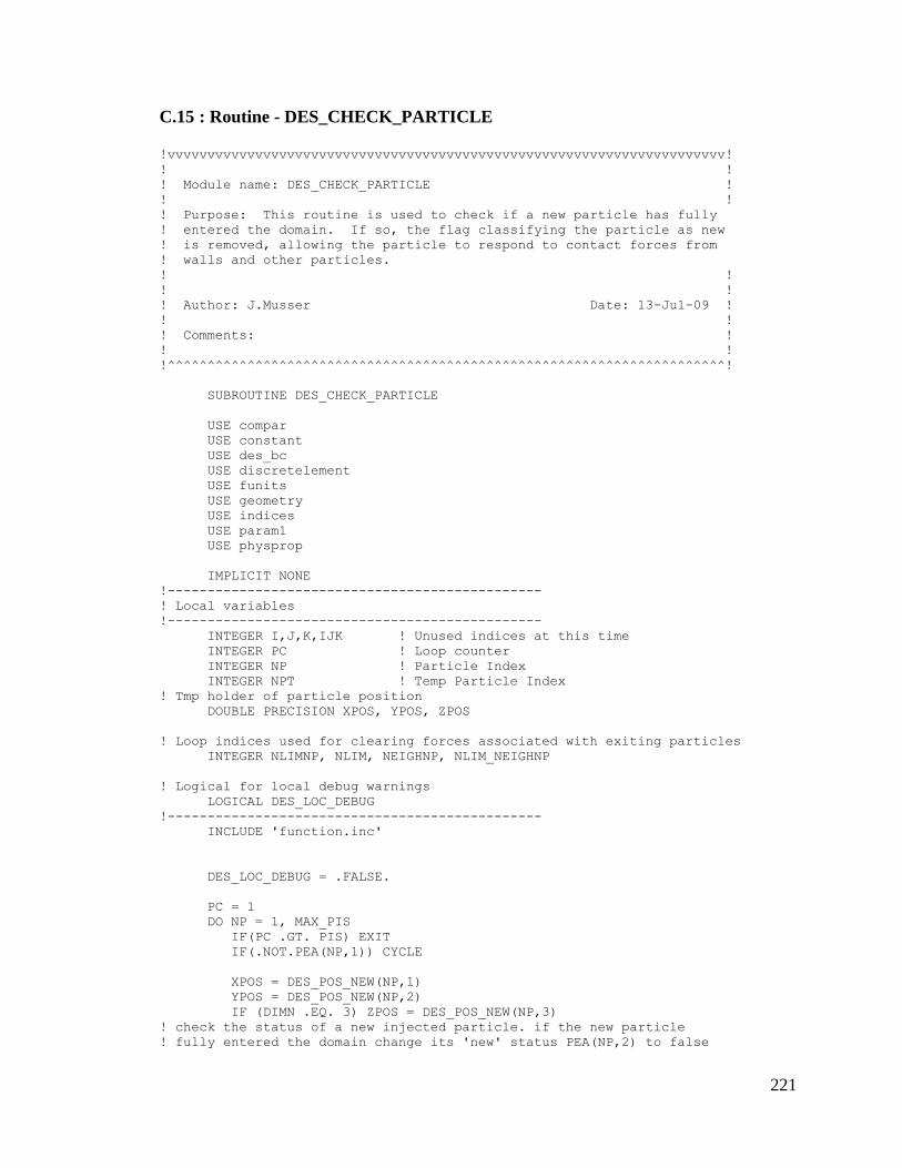
221

C.15 : Routine - DES_CHECK_PARTICLE


! !

! Module name: DES_CHECK_PARTICLE !

! !

! Purpose: This routine is used to check if a new particle has fully

! entered the domain. If so, the flag classifying the particle as new

! is removed, allowing the particle to respond to contact forces from

! walls and other particles.

! !

! !


! !

! Comments: !

! !

!^^^^^^^^^^^^^^^^^^^^^^^^^^^^^^^^^^^^^^^^^^^^^^^^^^^^^^^^^^^^^^^^^^^^^^!

SUBROUTINE DES_CHECK_PARTICLE

USE compar

USE constant

USE des_bc

USE discretelement

USE funits

USE geometry

USE indices

USE param1

USE physprop

IMPLICIT NONE

!-----------------------------------------------

! Local variables

!-----------------------------------------------

INTEGER I,J,K,IJK ! Unused indices at this time

INTEGER PC ! Loop counter

INTEGER NP ! Particle Index

INTEGER NPT ! Temp Particle Index

! Tmp holder of particle position

DOUBLE PRECISION XPOS, YPOS, ZPOS

! Loop indices used for clearing forces associated with exiting particles

INTEGER NLIMNP, NLIM, NEIGHNP, NLIM_NEIGHNP

! Logical for local debug warnings

LOGICAL DES_LOC_DEBUG

!-----------------------------------------------


DES_LOC_DEBUG = .FALSE.

PC = 1

DO NP = 1, MAX_PIS

IF(PC .GT. PIS) EXIT

IF(.NOT.PEA(NP,1)) CYCLE



IF (DIMN .EQ. 3) ZPOS = DES_POS_NEW(NP,3)

! check the status of a new injected particle. if the new particle

! fully entered the domain change its 'new' status PEA(NP,2) to false

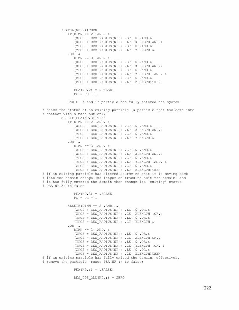
222

IF(PEA(NP,2))THEN

IF(DIMN == 2 .AND. &

(XPOS - DES_RADIUS(NP)) .GT. 0 .AND.&

(XPOS + DES_RADIUS(NP)) .LT. XLENGTH.AND.&

(YPOS - DES_RADIUS(NP)) .GT. 0 .AND.&

(YPOS + DES_RADIUS(NP)) .LT. YLENGTH &

.OR. &

DIMN == 3 .AND. &




(YPOS + DES_RADIUS(NP)) .LT. YLENGTH .AND. &

(ZPOS - DES_RADIUS(NP)) .GT. 0 .AND.&

(ZPOS + DES_RADIUS(NP)) .LT. ZLENGTH)THEN

PEA(NP,2) = .FALSE.

PC = PC + 1

ENDIF ! end if particle has fully entered the system

! check the status of an exiting particle (a particle that has come into

! contact with a mass outlet).

ELSEIF(PEA(NP,3))THEN

IF(DIMN == 2 .AND. &




(YPOS + DES_RADIUS(NP)) .LT. YLENGTH &

.OR. &

DIMN == 3 .AND. &




(YPOS + DES_RADIUS(NP)) .LT. YLENGTH .AND. &

(ZPOS - DES_RADIUS(NP)) .GT. 0 .AND.&

(ZPOS + DES_RADIUS(NP)) .LT. ZLENGTH)THEN

! if an exiting particle has altered course so that it is moving back

! into the domain change (no longer on track to exit the domain) and

! it has fully entered the domain then change its 'exiting' status

! PEA(NP,3) to false

PEA(NP,3) = .FALSE.

PC = PC + 1

ELSEIF(DIMN == 2 .AND. &

(XPOS + DES_RADIUS(NP)) .LE. 0 .OR.&

(XPOS - DES_RADIUS(NP)) .GE. XLENGTH .OR.&

(YPOS + DES_RADIUS(NP)) .LE. 0 .OR.&

(YPOS - DES_RADIUS(NP)) .GT. YLENGTH &

.OR. &

DIMN == 3 .AND. &

(XPOS + DES_RADIUS(NP)) .LE. 0 .OR.&

(XPOS - DES_RADIUS(NP)) .GE. XLENGTH.OR.&

(YPOS + DES_RADIUS(NP)) .LE. 0 .OR.&

(YPOS - DES_RADIUS(NP)) .GE. YLENGTH .OR. &

(ZPOS + DES_RADIUS(NP)) .LE. 0 .OR.&

(ZPOS - DES_RADIUS(NP)) .GE. ZLENGTH)THEN

! if an exiting particle has fully exited the domain, effectively

! remove the particle (reset PEA(NP,:) to false)

PEA(NP,:) = .FALSE.

DES_POS_OLD(NP,:) = ZERO

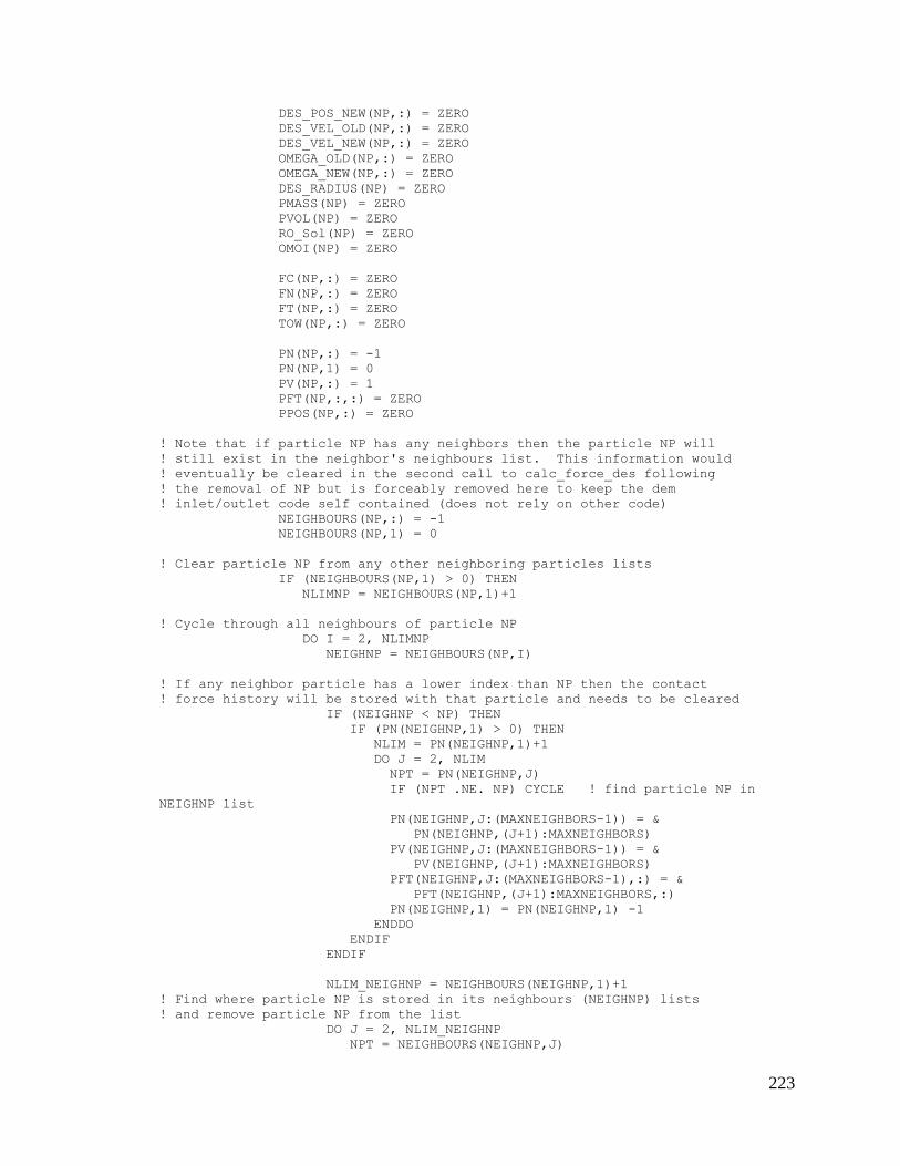
223

DES_POS_NEW(NP,:) = ZERO

DES_VEL_OLD(NP,:) = ZERO

DES_VEL_NEW(NP,:) = ZERO

OMEGA_OLD(NP,:) = ZERO

OMEGA_NEW(NP,:) = ZERO

DES_RADIUS(NP) = ZERO

PMASS(NP) = ZERO

PVOL(NP) = ZERO

RO_Sol(NP) = ZERO

OMOI(NP) = ZERO

FC(NP,:) = ZERO

FN(NP,:) = ZERO

FT(NP,:) = ZERO

TOW(NP,:) = ZERO

PN(NP,:) = -1

PN(NP,1) = 0

PV(NP,:) = 1

PFT(NP,:,:) = ZERO

PPOS(NP,:) = ZERO

! Note that if particle NP has any neighbors then the particle NP will

! still exist in the neighbor's neighbours list. This information would

! eventually be cleared in the second call to calc_force_des following

! the removal of NP but is forceably removed here to keep the dem

! inlet/outlet code self contained (does not rely on other code)

NEIGHBOURS(NP,:) = -1

NEIGHBOURS(NP,1) = 0

! Clear particle NP from any other neighboring particles lists

IF (NEIGHBOURS(NP,1) > 0) THEN

NLIMNP = NEIGHBOURS(NP,1)+1

! Cycle through all neighbours of particle NP

DO I = 2, NLIMNP

NEIGHNP = NEIGHBOURS(NP,I)

! If any neighbor particle has a lower index than NP then the contact

! force history will be stored with that particle and needs to be cleared

IF (NEIGHNP < NP) THEN

IF (PN(NEIGHNP,1) > 0) THEN

NLIM = PN(NEIGHNP,1)+1

DO J = 2, NLIM

NPT = PN(NEIGHNP,J)

IF (NPT .NE. NP) CYCLE ! find particle NP in

NEIGHNP list

PN(NEIGHNP,J:(MAXNEIGHBORS-1)) = &

PN(NEIGHNP,(J+1):MAXNEIGHBORS)

PV(NEIGHNP,J:(MAXNEIGHBORS-1)) = &

PV(NEIGHNP,(J+1):MAXNEIGHBORS)

PFT(NEIGHNP,J:(MAXNEIGHBORS-1),:) = &

PFT(NEIGHNP,(J+1):MAXNEIGHBORS,:)

PN(NEIGHNP,1) = PN(NEIGHNP,1) -1

ENDDO

ENDIF

ENDIF

NLIM_NEIGHNP = NEIGHBOURS(NEIGHNP,1)+1

! Find where particle NP is stored in its neighbours (NEIGHNP) lists

! and remove particle NP from the list

DO J = 2, NLIM_NEIGHNP

NPT = NEIGHBOURS(NEIGHNP,J)

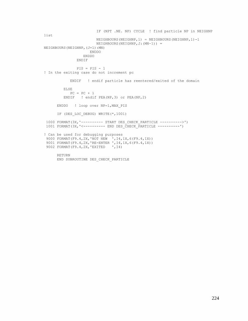
224

IF (NPT .NE. NP) CYCLE ! find particle NP in NEIGHNP

list

NEIGHBOURS(NEIGHNP,1) = NEIGHBOURS(NEIGHNP,1)-1

NEIGHBOURS(NEIGHNP,J:(MN-1)) =

NEIGHBOURS(NEIGHNP,(J+1):MN)

ENDDO

ENDDO

ENDIF

PIS = PIS - 1

! In the exiting case do not increment pc

ENDIF ! endif particle has reentered/exited of the domain

ELSE

PC = PC + 1

ENDIF ! endif PEA(NP,3) or PEA(NP,2)

ENDDO ! loop over NP=1,MAX_PIS

IF (DES_LOC_DEBUG) WRITE(*,1001)

1000 FORMAT(3X,'---------- START DES_CHECK_PARTICLE ---------->')

1001 FORMAT(3X,'<---------- END DES_CHECK_PARTICLE ----------')

! Can be used for debugging purposes

9000 FORMAT(F9.4,2X,'NOT NEW ',I4,1X,6(F9.4,1X))

9001 FORMAT(F9.4,2X,'RE-ENTER ',I4,1X,6(F9.4,1X))

9002 FORMAT(F9.4,2X,'EXITED ',I4)

RETURN

END SUBROUTINE DES_CHECK_PARTICLE

225

C.16 : Routine - DES_MASS_OUTLET


! !

! Module name: DES_MASS_OUTLET(NP, BCC, WC) !

! !

! Purpose: !

! Check if the particle's position overlaps the outlet position

! by more than its radius (i.e., the particle is more than just

! touching the boundary)

! !


! !

! Comments: !

! !

!^^^^^^^^^^^^^^^^^^^^^^^^^^^^^^^^^^^^^^^^^^^^^^^^^^^^^^^^^^^^^^^^^^^^^^!

SUBROUTINE DES_MASS_OUTLET(NP, BCC, WC)

USE des_bc

USE discretelement

USE param1

IMPLICIT NONE

!-----------------------------------------------

! Local variables

!-----------------------------------------------

INTEGER NP ! Particle ID Number

INTEGER WC ! Wall contact value (0: No Contact, 1: Contact)

INTEGER BCV_I, BCV

DOUBLE PRECISION XPOS, YPOS, ZPOS ! particle x,y,z position

DOUBLE PRECISION RAD ! particle radius

CHARACTER*2 BCC ! Boundary condition class (Xw,Xe,Ys,Yn,Zb,Zt)

!-----------------------------------------------

RAD = DES_RADIUS(NP)




ZPOS = ONE

ELSE

ZPOS = DES_POS_NEW(NP,3)

ENDIF

! Set the flag identifying a wall contact to 1 (contact exists). If the

! particle is in contact with a region of the wall that is listed as an

! outlet for DES particles, then the wall contact is ignored by setting

! the flag back to zero.

WC = 1

! Loop over all outflow boundary conditions

DO BCV_I = 1, DES_BCMO

BCV = DES_BC_MO_ID(BCV_I)

! Find which outlet boundary(s) index coincide with the passed boundary

! condition class.

IF(DES_MO_CLASS(BCV_I) == BCC)THEN

226


IF(BCC == 'XW' .OR. BCC == 'XE')THEN

IF(DES_BC_Y_s(BCV) < (YPOS - RAD) .AND. &

DES_BC_Y_n(BCV) > (YPOS + RAD) )THEN

WC = 0

PEA(NP,3) = .TRUE.

ENDIF

ENDIF

IF(BCC == 'YS' .OR. BCC == 'YN' )THEN

IF(DES_BC_X_w(BCV) < (XPOS - RAD) .AND. &

DES_BC_X_e(BCV) > (XPOS + RAD) )THEN

WC = 0

PEA(NP,3) = .TRUE.

ENDIF

ENDIF

ELSE ! 3D domain

IF(BCC == 'XW' .OR. BCC == 'XE')THEN

IF(DES_BC_Y_s(BCV) < (YPOS - RAD) .AND. &

DES_BC_Y_n(BCV) > (YPOS + RAD) .AND. &

DES_BC_Z_b(BCV) < (ZPOS - RAD) .AND. &

DES_BC_Z_t(BCV) > (ZPOS + RAD) )THEN

WC = 0

PEA(NP,3) = .TRUE.

ENDIF

ENDIF

IF(BCC == 'YS' .OR. BCC == 'YN')THEN


DES_BC_X_e(BCV) > (XPOS + RAD) .AND. &

DES_BC_Z_b(BCV) < (ZPOS - RAD) .AND. &

DES_BC_Z_t(BCV) > (ZPOS + RAD) )THEN

WC = 0

PEA(NP,3) = .TRUE.

ENDIF

ENDIF

IF(BCC == 'ZB' .OR. BCC == 'ZT')THEN


DES_BC_X_e(BCV) > (XPOS + RAD) .AND. &

DES_BC_Y_s(BCV) < (YPOS - RAD) .AND. &

DES_BC_Y_n(BCV) > (YPOS + RAD) )THEN

WC = 0

PEA(NP,3) = .TRUE.

ENDIF

ENDIF

ENDIF ! endif dimn == 2

ENDIF ! endif DES_MO_CLASS(BCV_I) == BCC

ENDDO ! loop over BCV_I the no. of outlet boundaries

9000 FORMAT(F9.4,2X,'PEA(3)=T ',I4,1X,6(F9.4,1X))

END SUBROUTINE DES_MASS_OUTLET

227

Appendix D: Particle heat transfer model source code

The section contains the source code for the particle heat transfer models. It has

been written in the FORTRAN90/95 style.

D.1 Module – DES_IC


! !

! Module name: DES_IC !

! !

! Purpose: Common elements needed for DES initial conditions. !

! !

! !

! Author: J.Musser Date: 17-Feb-11 !

! !

! Comments: !

! !

!^^^^^^^^^^^^^^^^^^^^^^^^^^^^^^^^^^^^^^^^^^^^^^^^^^^^^^^^^^^^^^^^^^^^^^!

MODULE DES_IC

USE param

! Logical variable to determine whether an initial condition is defined

LOGICAL DES_IC_DEFINED (DIMENSION_IC)

! Set to true if any DES initial condition regions are specified. This

! logical is used to invoke the call to DES_SET_IC.

LOGICAL DES_IC_EXIST

! Physical coordinates indicating initial condition region

DOUBLE PRECISION DES_IC_X_w(DIMENSION_IC)

DOUBLE PRECISION DES_IC_X_e(DIMENSION_IC)

DOUBLE PRECISION DES_IC_Y_s(DIMENSION_IC)

DOUBLE PRECISION DES_IC_Y_n(DIMENSION_IC)

DOUBLE PRECISION DES_IC_Z_b(DIMENSION_IC)

DOUBLE PRECISION DES_IC_Z_t(DIMENSION_IC)

! Initial solids phase temperature in a specified region

DOUBLE PRECISION DES_IC_T_s (DIMENSION_IC, DIM_M)

! Initial solids species mass fractions in a specified region

DOUBLE PRECISION DES_IC_X_s (DIMENSION_IC, DIM_M, DIM_N_s)

! Density of unreacted, shrinking core

DOUBLE PRECISION DES_IC_CORE_Rho(DIMENSION_IC, DIM_M)

END MODULE DES_IC

228

D.2 Routine – CHECK_DES_IC


! !

! Module name: CHECK_DES_IC !

! !

! Purpose: Check the data provided for des initial conditions. !

! !

! !


! !

! Comments: !

! !

!^^^^^^^^^^^^^^^^^^^^^^^^^^^^^^^^^^^^^^^^^^^^^^^^^^^^^^^^^^^^^^^^^^^^^^!

SUBROUTINE CHECK_DES_IC

USE des_ic

USE discretelement

USE param

USE param1

USE des_thermo

USE des_rxns

USE compar

USE constant

USE funits

USE geometry

USE indices

USE physprop

USE run

IMPLICIT NONE

INTEGER ICV

!-----------------------------------------------


!-----------------------------------------------


!-----------------------------------------------

WRITE(*,'(1X,A)') '---------- START CHECK_DES_IC ---------->'

! Initialize the initial condition logical.

DES_IC_EXIST = .FALSE.

! Check for des inlet/outlet information:

CHECK_IC: DO ICV = 1, DIMENSION_IC

DES_IC_DEFINED(ICV) = .FALSE.

IF (DES_IC_X_w(ICV) /= UNDEFINED) DES_IC_DEFINED(ICV) = .TRUE.

IF (DES_IC_X_e(ICV) /= UNDEFINED) DES_IC_DEFINED(ICV) = .TRUE.

IF (DES_IC_Y_s(ICV) /= UNDEFINED) DES_IC_DEFINED(ICV) = .TRUE.

IF (DES_IC_Y_n(ICV) /= UNDEFINED) DES_IC_DEFINED(ICV) = .TRUE.

IF (DES_IC_Z_b(ICV) /= UNDEFINED) DES_IC_DEFINED(ICV) = .TRUE.

IF (DES_IC_Z_t(ICV) /= UNDEFINED) DES_IC_DEFINED(ICV) = .TRUE.

! If an initial condition is specified, verify necessary data

! Check that all dimensions have been defined

IF (DES_IC_DEFINED(ICV)) THEN

IF(DES_IC_X_w(ICV) == UNDEFINED .OR. &

DES_IC_X_e(ICV) == UNDEFINED .OR. &

229

DES_IC_Y_s(ICV) == UNDEFINED .OR. &

DES_IC_Y_n(ICV) == UNDEFINED) THEN

WRITE (UNIT_LOG, 1000) ICV

WRITE (*, 1000) ICV


ENDIF

IF(DIMN == 3)THEN

IF(DES_IC_Z_b(ICV) == UNDEFINED .OR. &

DES_IC_Z_t(ICV) == UNDEFINED) THEN


WRITE (*, 1000) ICV


ENDIF

ENDIF

! Check that the region does not overlap

IF(DES_IC_X_w(ICV) .LT. ZERO .OR. &

DES_IC_Y_s(ICV) .LT. ZERO .OR. &

DES_IC_X_e(ICV) .GT. XLENGTH .OR. &

DES_IC_Y_n(ICV) .GT. YLENGTH .OR. &

DES_IC_X_w(ICV) .GT. DES_IC_X_e(ICV) .OR. &

DES_IC_Y_s(ICV) .GT. DES_IC_Y_n(ICV))THEN


WRITE (*, 1001) ICV


ENDIF

IF(DIMN == 3)THEN

IF(DES_IC_Z_b(ICV) .LT. 0 .OR. &

DES_IC_Z_t(ICV) .GT. ZLENGTH .OR. &

DES_IC_Z_b(ICV) .GT. DES_IC_Z_t(ICV))THEN


WRITE (*, 1001)ICV


ENDIF

ENDIF

! This is used to invoke the call to DES_SET_IC which is only done

! if there are valid initial conditions specified.

DES_IC_EXIST = .TRUE.

ENDIF ! end if DES_IC_DEFINED(ICV)

ENDDO CHECK_IC

! If the DES energy equations or DES species equation are being solve

! then initial conditions must be specified to provide the intial

! sate of the particles.

IF(.NOT.DES_IC_EXIST) THEN

IF(DES_ENERGY_EQ) THEN

WRITE(*,1002)'temperature','energy equation'



ELSEIF(ANY_DES_SPECIES_EQ) THEN

WRITE(*,1002)'species mass fractions','species equation'



ENDIF

ENDIF

WRITE(*,'(1X,A)') '<---------- END CHECK_DES_IC ----------'

1000 FORMAT(/1X,70('*')/, ' From: CHECK_DES_IC',/, ' Message: ',&

230

'Insufficient DEM initial condition infomation',/10X,&

'Check initial condition number: ',I3,/1X,70('*')/)

1001 FORMAT(/1X,70('*')/, ' From: CHECK_DES_IC',/, ' Messsage: ',&

'Improper DEM initial condition information',/10X,&

'Check initial condition number: ',I3,/1X,70('*')/)

1002 FORMAT(/1X,70('*')/,' From: CHECK_DES_IC',/'Message: Initial', &

' condition data specifying the paritcle',/A,' is requied', &

' when solving the ',A,'.',/' Check mfix.dat.',/1X,70('*')/)

RETURN

END SUBROUTINE CHECK_DES_IC

231

D.3 Routine – DES_SET_IC


! !

! SUBROUTINE Name: DES_SET_IC !

! !

! Purpose: Assign initial conditions to particles basded upon thier !

! location within the domain. !

! !


! !

! Comments: !

! !

!^^^^^^^^^^^^^^^^^^^^^^^^^^^^^^^^^^^^^^^^^^^^^^^^^^^^^^^^^^^^^^^^^^^^^^!

SUBROUTINE DES_SET_IC

USE compar

USE des_thermo

USE discretelement

USE des_ic

USE des_rxns

USE funits

IMPLICIT NONE

! Dummy indices

INTEGER PC, I, M, ICV

! X,Y, and Z values of particle position

DOUBLE PRECISION X_POS, Y_POS, Z_POS

! Logical indicating that no IC was define in the region containing

! the specified particle.

LOGICAL IC_FOUND


! Loop through the particles in the system, skipping entring, exiting

! and "non-existing" particles.

PC = 1

DO I = 1, MAX_PIS


IF(.NOT.PEA(I,1)) CYCLE

! Set the solids phase of the particle

M = PIJK(I,5)

X_POS = DES_POS_NEW(I,1)

Y_POS = DES_POS_NEW(I,2)

IF(DIMN == 3) Z_POS = DES_POS_NEW(I,3)

IC_FOUND = .FALSE.

! Loop through the initial conditions

DO ICV = 1, DIMENSION_IC

IF (DES_IC_DEFINED(ICV)) THEN

! Check to see if the position of the particle is located inside the

! initial condition region.

IF(X_POS .GE. DES_IC_X_W(ICV) .AND. &

X_POS .LE. DES_IC_X_E(ICV) .AND. &

Y_POS .GE. DES_IC_Y_S(ICV) .AND. &

Y_POS .LE. DES_IC_Y_N(ICV) ) THEN

IF(DIMN == 2 .OR. &

(Z_POS .GE. DES_IC_Z_B(ICV) .AND. &

232

Z_POS .LE. DES_IC_Z_T(ICV)) ) THEN

ENDIF

! Change the flag to indicate that an IC regioon has been found.

IC_FOUND = .TRUE.

! Exit the loop and assign the initial conditions to particle I.

EXIT

ENDIF

ENDIF

ENDDO

IF(IC_FOUND)THEN

! Assign the initial values for the specified models.

CALL SET_DES_TEMPERATURE(I,ICV,M)

CALL SET_DES_MASS_FRACTION(I,ICV,M)

CALL SET_DES_CORE_DENSITY(I,ICV,M)

ELSE

IF(DIMN == 2) Z_POS = 0.0d0

WRITE(*,1000)I, X_POS, Y_POS, Z_POS

WRITE(UNIT_LOG,1000)I, X_POS, Y_POS, Z_POS


ENDIF

! icrement the particle counter

PC = PC + 1

ENDDO

1000 FORMAT(/1X,70('*')/,' From: SET_DES_IC',/, ' Message:', &

' There is no initial condition associated with the region',/ &

' containing particle ',I6,'.',/,' X Position: ',F9.4, / &

' Y Position: ',F9.4,/' Z Position: ',F9.4,/' Please check', &

' the mfix.dat file.',/ &

1X,70('*')/)

CONTAINS

!......................................................................!

! Subroutine: SET_DES_TEMPERATURE !

! !

! Purpose: Set the initial temperature of a partile. !

!``````````````````````````````````````````````````````````````````````!

SUBROUTINE SET_DES_TEMPERATURE(I,ICV,M)

INTEGER, INTENT(IN) :: I, ICV, M

! Initial temperatures must be specified for particles when solving

! the internal energy equation and species equation for a particle.

IF(.NOT.ANY_DES_SPECIES_EQ .AND. .NOT.DES_ENERGY_EQ ) RETURN

IF(DES_IC_T_s(ICV,M) == UNDEFINED) THEN

WRITE(*,1000)ICV,M,I

WRITE(UNIT_LOG,1000)ICV,M,I


ELSE

DES_T_s_NEW(I) = DES_IC_T_s(ICV,M)

ENDIF

! Set the value of the old temperature to the initial value.

DES_T_s_OLD(I) = DES_T_s_NEW(I)

RETURN

1000 FORMAT(/1X,70('*')/,' From: SET_DES_IC',/, ' Message: The', &

' initial temperature is UNDEFINED for particle ',I6,'.',/ &

' This is required when solving the internal energy equation',&

' and species',/' equation for a particle. Check mfix.dat', &

233

' file.',/1X,70('*')/)

END SUBROUTINE SET_DES_TEMPERATURE

!......................................................................!

! Subroutine: SET_DES_MASS_FRAC !

! !

! Purpose: Set the initial species mass fraction of a partile. !

!``````````````````````````````````````````````````````````````````````!

SUBROUTINE SET_DES_MASS_FRACTION(I,ICV,M)


INTEGER N ! species loop index

DOUBLE PRECISION SUM

! The initial species mass fractions for a particle must be supplied if

! the species equation is being solved or if DES_C_PS0 has not been

! specified in conjunction with the energy equations being solved.

IF(.NOT.ANY_DES_SPECIES_EQ .AND. (.NOT.DES_ENERGY_EQ .OR. &

(DES_ENERGY_EQ .AND. DES_C_PS0(M) /= UNDEFINED) ) ) RETURN

! Verify that the species mass fraction sums to one.

SUM = ZERO

DO N=1,DES_NMAX(M)

IF(DES_IC_X_s(ICV,M,N) /= UNDEFINED) THEN

DES_X_s(I,N) = DES_IC_X_s(ICV,M,N)

SUM = SUM + DES_IC_X_s(ICV,M,N)

ELSE

DES_X_s(I,N) = ZERO

ENDIF

ENDDO

IF(.NOT.COMPARE(ONE,SUM))THEN

WRITE(*,1000)I

WRITE(UNIT_LOG,1000)I


ENDIF

RETURN

1000 FORMAT(/1X,70('*')/,' From: SET_DES_IC',/, ' Message: The', &

' species mass fraction of particle ',I6,' does not sum',/ &

' to one. This is required if sovling the discrete particle', &

' species',/' equation or if DES_C_PS0 is not specified when',&

' solving the internal',/' energy equation for a particle.', &

' Check mfix.dat file.',/1X,70('*')/)

END SUBROUTINE SET_DES_MASS_FRACTION

!......................................................................!

! Subroutine: SET_DES_CORE_DENSITY !

! !

! Purpose: Set the denisty of shrinking, unreacted core of a partile. !

!``````````````````````````````````````````````````````````````````````!

SUBROUTINE SET_DES_CORE_DENSITY(I,ICV,M)


! Error indicating that an error has been specified to the user.

LOGICAL, SAVE :: WARNED = .FALSE.

! Set the density of the unreacted core for reactive gas-solid flows.

! This value is *optional* but effects how the radius of the core

! changes during a reaction. If a value is not provided in the mfix.dat

234

! file, the density of the particle is assigned to the core.

IF(.NOT.DES_SPECIES_EQ(M) .OR. TRIM(REACTION_MODEL) /= &

'SHRINKING_CORE') RETURN

IF(DES_IC_CORE_Rho(ICV,M) == UNDEFINED) THEN

IF(.NOT.WARNED)THEN

WRITE(*,1000)


WARNED = .TRUE.

ENDIF

CORE_Rho(I) = RO_Sol(I)

ELSE

CORE_Rho(I) = DES_IC_CORE_Rho(ICV,M)

ENDIF

RETURN

1000 FORMAT(/1X,70('*')/,' From: SET_DES_IC',/, ' Message: Some or', &

' all of the discrete solids phases do not have an',/ &

' initial core density defined. This effects how the', &

' shrinking,',/,' unreacted core model behaves.',/,' The', &

' core density will be set to the particle density.',/, &

1X,70('*')/)

END SUBROUTINE SET_DES_CORE_DENSITY

END SUBROUTINE DES_SET_IC

235

D.4 Module – DES_THERMO


! !

! Module name: DES_THERMO !

! !

! Purpose: Common elements for MFIX-DEM heat transfer. !

! condition. !

! !

! Author: J.Musser Date: 16-Jun-10 !

! !

! Comments: !

! !

!^^^^^^^^^^^^^^^^^^^^^^^^^^^^^^^^^^^^^^^^^^^^^^^^^^^^^^^^^^^^^^^^^^^^^^!

MODULE DES_THERMO

USE param

! Run time logicals

!--------------------------

! Slove DES Energy Equations

LOGICAL DES_ENERGY_EQ

! Specifies that the convection model is to be solved.

! Requires DES_ENERGY_EQ = .TRUE.

! Default [.TRUE.]

LOGICAL DES_CONV_EQ

! Specifies that the particle conduction models are to be solved.

! Requires DES_ENERGY_EQ = .TRUE.

! Default [.TRUE.]

LOGICAL DES_COND_EQ

! These logicals can be set in the mfix.dat file to omit specific

! particle-particle heat conduction models from being solved.

! If the DEM conduction model is not solved (DES_COND_EQ), the values

! are automatically set to .FALSE. in check_des_thermo.f.

! Default [.TRUE.]

LOGICAL DES_COND_EQ_PFP ! particle-fluid-particle

! Default [.TRUE.]

LOGICAL DES_COND_EQ_PP ! particle-particle

! Specifies that the particle-environment radiation model is to be

! solved. Requires DES_ENERGY_EQ = .TRUE.

! Default [.TRUE.]

LOGICAL DES_RADI_EQ

! Heat transfer correlation specified in mfix.dat

! Default [RANZ_1952]

CHARACTER*24 :: DES_CONV_CORR

! Specifies that a thermodynamic neighborhood for a particle be

! determined. This neighborhood can be much larger than the one

! established for determining collisions. It is used in conduction and

! radiation models.

LOGICAL FIND_THERMO_NBRHD

! Particle properties

!--------------------------

! Particle temperature at current time step (S_TIME)

DOUBLE PRECISION, DIMENSION(:), ALLOCATABLE :: DES_T_s_OLD !(PARTICLES)

! Particle temperature at previous time step (S_TIME - DT_SOLID)

DOUBLE PRECISION, DIMENSION(:), ALLOCATABLE :: DES_T_s_NEW !(PARTICLES)

236

! DES Specified constant solids thermal conductivity by solids phase

DOUBLE PRECISION DES_K_s0(DIM_M)

! DES solids thermal conductivity by particle ! (not currently used)

DOUBLE PRECISION, DIMENSION(:), ALLOCATABLE :: DES_K_s

! DES Specified constant solids specific heat by solids phase

DOUBLE PRECISION DES_C_ps0(DIM_M)

! DES specific heat of particles by particle

DOUBLE PRECISION, DIMENSION(:), ALLOCATABLE :: DES_C_ps

! Emissivity of particles

DOUBLE PRECISION DES_Em(DIM_M)

! Stefan-Boltzmann Constant

DOUBLE PRECISION SB_CONST

! Rates of heat transfer

!--------------------------

! Heat transfer TO the particle from the fluid. This value will be positive

! when the particle is heating and negative when the particle is cooling.

DOUBLE PRECISION, DIMENSION(:), ALLOCATABLE :: Qcv !(PARTICLES)

! Heat transfer TO the particle from neighboring particles via the particle-

! particle conduction model. This value will be positive when the particle is

! heating and negative when the particle is cooling.

DOUBLE PRECISION, DIMENSION(:), ALLOCATABLE :: Qpp !(PARTICLES)

! Heat transfer TO the particle from neighboring particles via the particle-

! fluid-particle model. This value will be positive when the particle is

! heating and negative when the particle is cooling.

DOUBLE PRECISION, DIMENSION(:), ALLOCATABLE :: Qpfp !(PARTICLES)

! Heat transfer TO the particle from neighboring particles via radiation

DOUBLE PRECISION, DIMENSION(:), ALLOCATABLE :: Qrd !(PARTICLES)

! Internal heat generation resulting from a chemical reaction

DOUBLE PRECISION, DIMENSION(:), ALLOCATABLE :: Qint !(PARTICLES)

! Previous time step's rate of heat transfer. Used for Adams-Bashforth

! time integration scheme

DOUBLE PRECISION, DIMENSION(:), ALLOCATABLE :: Qtotal_OLD

! Thermodynamic Neighborhood

!--------------------------

! Thermodynamic neighborhood. This is the list of particles around a

! particle that may transfer energy with the given particle.

INTEGER, DIMENSION(:,:), ALLOCATABLE :: THERMO_NBRHD ! (PARTICLES,

MAXNEIGHBORS)

! This is the size of the thermodynamic neighborhood. Is is based on the

! maximum particle radius and the FLPC and RDPC

DOUBLE PRECISION NBRHD_SZ

! Fluid Lens Proportion Constant used to calculate the radius of the

! fluid lens that surrounds the particle for particle-fluid-particle

! conduction. Default [ 0.2 ]

DOUBLE PRECISION FLPC

! Radius of the radiation domain in relation of the particle diameter.

! Default [ 3.0 ] * DES_RADIUS(-)

DOUBLE PRECISION RDPC

! Mininum separation distance between the surface of two contacting

! particles. This value is used to remove the singluarity that the

! particle-fluid-particle conduciton model develops at the contact

! interface. [4.0x10^(-10) meters]

DOUBLE PRECISION DES_MIN_COND_DIST

END MODULE DES_THERMO

237

D.5 Routine – CHECK_DES_THERMO


! !

! Module name: CHECK_DES_THERMO !

! !

! Purpose: !

! !

! !


! !

! Comments: !

! !

!^^^^^^^^^^^^^^^^^^^^^^^^^^^^^^^^^^^^^^^^^^^^^^^^^^^^^^^^^^^^^^^^^^^^^^!

SUBROUTINE CHECK_DES_THERMO

Use compar

Use des_thermo

Use discretelement

Use funits

Use interpolation

Use physprop

Use run

IMPLICIT NONE

!-----------------------------------------------

! Local variables

!-----------------------------------------------

INTEGER I, M ! dummy loop index

! The size of the thermodynamic neighborhoods needed for particle-fluid-

! particle conduction and radiation.

DOUBLE PRECISION SZ_PFP, SZ_RAD

!-----------------------------------------------

! Functions

!-----------------------------------------------

WRITE(*,'(1X,A)')&

'---------- START CHECK_DES_THERMO ---------->'

IF(DES_ENERGY_EQ)THEN

! Loop over all solids phases

DO M=1,MMAX

! Verify that the thermal conductivity values are physical.

IF(DES_C_ps0(M) .LT. ZERO)THEN

WRITE(UNIT_LOG,1001)'DES_C_ps0','unphysical',M

WRITE(*,1001)'DES_C_ps0','unphysical',M


ENDIF

! Verify that the thermal conductivity values are physical and defined.

IF(DES_K_s0(M) .LT. ZERO)THEN

WRITE(UNIT_LOG,1001)'DES_K_s0','unphysical',M

WRITE(*,1001)'DES_K_s0','unphysical',M


ELSEIF(DES_K_s0(M) == UNDEFINED)THEN

WRITE(UNIT_LOG,1001)'DES_K_s0','undefined',M

WRITE(*,1001)'DES_K_s0','undefined',M


ENDIF

ENDDO

238

! Convection Equation:

!'''''''''''''''''''''''''''''''''''''''''''''''''''''''''''''''''''''''

IF(DES_CONV_EQ) THEN

! Ensure that the continuum energy equations will be solved.

IF(.NOT.ENERGY_EQ)THEN

WRITE(*,1000)


ENDIF

WRITE(*,'(6X,A)') 'DES convection model will be solved.'

SELECT CASE(TRIM(DES_CONV_CORR))

! Verify the selected convective heat transfer coefficient model

CASE ('RANZ_1952')

! Ranz, W.E. and Marshall, W.R., "Frication and transfer

! coefficients for single particles and packed beds,"

! Chemical Engineering Science, Vol. 48, No. 5, pp 247-253,

! 1925

! The Ranz and Marshall correlation needs no additional input from the

! user.

WRITE(*,'(9X,A,A)')'Heat transfer coefficient',&

' model: Ranz and Marshall (1952)'

! If the heat transfer coefficient correlation provided by the user does

! not match one of the models outlined above, flag the error and exit.

CASE DEFAULT

WRITE(*,'(6X,A)') &

'INVALID DES CONVECTION MODEL (DES_CONV_CORR):'

WRITE(*,'(6X,A)')'The available models include:'

WRITE(*,'(9X,A)')'RANZ_1952 - Ranz and Marshall (1952)'

CALL MFIX_EXIT

END SELECT

ELSE

WRITE(*,'(6X,A)') 'DES convection model will NOT be solved.'

ENDIF ! END convection model checks

! Conduction Equations:

!'''''''''''''''''''''''''''''''''''''''''''''''''''''''''''''''''''''''

IF(DES_COND_EQ) THEN

WRITE(*,'(6X,A)') 'DES conduction model will be solved.'

! Particle-particle Conduction:

!'''''''''''''''''''''''''''''''''''''''''''''''''''''''''''''''''''''''

IF(DES_COND_EQ_PP) THEN

DO M=1,MMAX

! Verify that a thermal conductivity value is specified for each solids

! phase and that the value is physical.

IF(DES_K_S0(M) == UNDEFINED)THEN

WRITE(UNIT_LOG,1001)'DES_K_s0','undefined',M

WRITE(*,1001)'DES_K_s0','undefined',M


ELSEIF(DES_K_S0(M) .LT. ZERO) THEN

WRITE(UNIT_LOG,1001)'DES_K_s0','unphysical',M

WRITE(*,1001)'DES_K_s0','unphysical',M


ENDIF

ENDDO

WRITE(*,'(6X,A)')&

'Solving the particle-particle conduction model.'

239

! A secondary neighborhood is established surrounding a particle to

! determine the neighboring particles for possible particle-particle

! heat transfer.

FIND_THERMO_NBRHD = .TRUE.

ELSE

WRITE(*,'(5X,A)')&

'NOT Solving the particle-particle conduction model.'

ENDIF

! Particle-fluid-particle Conduction:

!'''''''''''''''''''''''''''''''''''''''''''''''''''''''''''''''''''''''

IF(DES_COND_EQ_PFP) THEN

! Verify that either the simulation is coupled with a gas-phase

! simulation or that K_g0 has been provided in the dat file.

IF(K_G0 == UNDEFINED .AND. &

.NOT.DES_CONTINUUM_COUPLED)THEN

WRITE(*,1002)



ENDIF

! Set the default value for the minimum distance separating particles'

! surfaces.

IF(DES_MIN_COND_DIST == UNDEFINED)THEN

DES_MIN_COND_DIST = 1.0D-04 ! cm

IF (UNITS == 'SI') DES_MIN_COND_DIST = &

DES_MIN_COND_DIST/100.0 ! m

ENDIF

WRITE(*,'(6X,A)')&

'Solving the particle-fluid-particle conduction model.'


! determine the neighboring particles for possible particle-fluid-

! particle heat transfer.


ELSE

WRITE(*,'(6X,A)')&

'NOT Solving the particle-fluid-particle conduction model.'

ENDIF

ELSE

WRITE(*,'(6X,A)') 'DES conduction model will NOT be solved.'

! Set the logicals for the conduction sub-models to false.

! This should not be needed, but is done for precaution.

DES_COND_EQ_PFP = .FALSE.

DES_COND_EQ_PP = .FALSE.

ENDIF ! END conduction model checks

! Radiation Equation:

!'''''''''''''''''''''''''''''''''''''''''''''''''''''''''''''''''''''''

IF(DES_RADI_EQ) THEN

WRITE(*,'(6X,A)') 'DES radiation model will be solved.'


! determine the neighboring particles for possible radiative

! heat transfer.


! Set the value of the Stefan-Boltzman Constant based on the untis

IF(UNITS == 'SI')THEN

! W/((m^2).K^4)

SB_CONST = 5.6704d0*(10.0d0**(-8))

ELSE

! cal/((cm^2).sec.K^4)

240

SB_CONST = 1.355282d0*(10.0d0**(-12))

ENDIF

DO M=1,MMAX

! Verify that a emmisivity value is specified for each solids pase

IF(DES_Em(M) == UNDEFINED)THEN

WRITE(UNIT_LOG,1001)'DES_Em','undefined',M

WRITE(*,1001)'DES_Em','undefined',M


ELSEIF(DES_Em(M) .LT. ZERO .OR. &

DES_Em(M) .GT. ONE) THEN

WRITE(UNIT_LOG,1001)'DES_Em','unphysical',M

WRITE(*,1001)'DES_Em','unphysical',M


ENDIF

ENDDO

ELSE

WRITE(*,'(6X,A)') 'DES radiation model will NOT be solved.'

ENDIF ! END radiation model checks

! Calculate the size of the thermodynamic neighbor (if needed)

IF( FIND_THERMO_NBRHD) THEN

SZ_PFP = ZERO

! If solving conductive heat transfer, the minimum neighborhood size

! is [1.3]*DES_RADIUS by default. A buffer of 0.1 is added to ensure

! that the neighbor is seen as soon as possible. The size of the fluid

! lens for particle-fluid-particle heat transfer can be adjusted by

! specifying a different value in the mfix.dat file.

IF(DES_COND_EQ_PP .OR. DES_COND_EQ_PFP) &

SZ_PFP = MAX_RADIUS * ( 2.05d0 + FLPC )

SZ_RAD = ZERO

! If radiation heat transfer is solved, the radius of the radiative

! heat transfer domain is [3.0]*DES_RADIUS by default. The size of the

! radiative heat transfer domain on the particle may be adjusted by

! specifying a new value in the mfix.dat file.

IF(DES_RADI_EQ) &

SZ_RAD = MAX_RADIUS * RDPC

NBRHD_SZ = MAX( SZ_PFP, SZ_RAD )

WRITE(*,'(6X,A,F10.6)') &

'Radius of thermodynamic neighborhood is ',NBRHD_SZ

ENDIF ! FIND_THERMO_NBRHD

ELSE ! DES_ENERGY_EQ

WRITE(*,'(6X,A)') 'DES energy equations are not being solved.'

! Reinitialize the heat transfer logicals to false.

DES_CONV_EQ = .FALSE.

DES_COND_EQ = .FALSE.

DES_RADI_EQ = .FALSE.

DES_COND_EQ_PFP = .FALSE.

DES_COND_EQ_PP = .FALSE.

ENDIF ! DES_ENERGY_EQ

WRITE(*,'(1X,A)')&

'<---------- END CHECK_DES_THERMO ----------'

RETURN

1000 FORMAT(/1X,70('*')/, ' From: CHECK_DES_THERMO',/, ' Message: ',&

'The DES convection model requires that the energy ', &

241

'equations',/1X,'(ENERGY_EQ) for the continuum phase must ',&

'also be solved.',/1X,70('*')/)

1001 FORMAT(/1X,70('*')/, ' From: CHECK_DES_THERMO',/, ' Message: ',&

A,' is ',A,' for solids phase ',I2,'. Check mfix.dat.', &

/1X,70('*')/)

1002 FORMAT(/1X,70('*')/,' From: CHECK_DES_THERMO',/,' Message:', &

' The particle-fluid-particle model requires that either a'/, &

' simulation be coupled with a gas-phase simultion or that', &

' K_g0 be',/,' provided in the mfix.dat file. Check mfix.dat.', &

/1X,70('*')/)

END SUBROUTINE CHECK_DES_THERMO

242

D.6 Routine – CALC_THERMO_DES


! !

! Module name: CALC_THERMO_DES !

! !

! Purpose: !

! !

! !


! !

! Comments: !

! !

!^^^^^^^^^^^^^^^^^^^^^^^^^^^^^^^^^^^^^^^^^^^^^^^^^^^^^^^^^^^^^^^^^^^^^^!

SUBROUTINE CALC_THERMO_DES(I, INTERP_IJK, INTERP_WEIGHTS, FOCUS)

Use des_thermo

Use discretelement

Use fldvar

Use interpolation

Use param1

IMPLICIT NONE

! Passed variables

!-----------------------------------------------

! Index of particle being looped over

INTEGER, INTENT(IN) :: I

! IJK indicies of fluid cells involved in interpolation

INTEGER, INTENT(IN) :: INTERP_IJK(INTERP_ORDER**DIMN)

! Weights associated with interpolation

DOUBLE PRECISION, INTENT(IN) :: INTERP_WEIGHTS(INTERP_ORDER**DIMN)

! Indicates that debugging information for the particle

LOGICAL, INTENT(IN) :: FOCUS

! Local variables

!-----------------------------------------------

! Index of neighbor particle of particle I such that I < J

INTEGER J

! Generic index of neighbor particle of particle I

INTEGER JJ

! index to track accounted for particles

INTEGER PC

! Number of particles in the radiation domain

INTEGER N_RAD

! Distance between the centers of particle I and particle J (component)

DOUBLE PRECISION DISTVEC(DIMN)

! Distance between the centers of particle I and particle J (magnitude)

DOUBLE PRECISION CENTER_DIST

! Distance between the surfaces of particle I and particle J

DOUBLE PRECISION SURFACE_DIST

! Angle generated between the line connecting the particle centers of

! particle I and J and the line generated by the center of particle I

! and one of the premiter of the circle generated by intersection area

! of particle I and particle J

DOUBLE PRECISION ANG_IJ

! Radius of the circle created by the overlap of the spherical particles

DOUBLE PRECISION R_sij

! Environment temperature used in the radiative heat transfer model

DOUBLE PRECISION Ts_RAD

243

! Functions

!-----------------------------------------------


! calculate heat transfer via convection

IF(DES_CONV_EQ) CALL DES_CONVECTION(I, INTERP_IJK, &

INTERP_WEIGHTS, FOCUS)

! Loop over thermodynamic neighbor for conduction and radiation

IF(DES_COND_EQ .OR. DES_RADI_EQ)THEN

! Initialize variables on entry

Ts_RAD = ZERO

N_RAD = 0

! Distance between particle centers

IF (THERMO_NBRHD(I,1).GT.0) THEN

DO JJ = 2, THERMO_NBRHD(I,1)+1

! Set the index of the neighbor particle

J = THERMO_NBRHD(I,JJ)

! Skip the neighbor if it does not exist (should not be a problem)

IF(.NOT.PEA(J,1) ) CYCLE

! Only do conduction calculations for particles with an index value

! higher than the current particle. The opposite heat transfer will be

! applied to the neighbor.

IF(J.GT.I) THEN

! Calculate the center distance between the two particles

DISTVEC(:) = DES_POS_NEW(I,:) - DES_POS_NEW(J,:)

CENTER_DIST = SQRT(DES_DOTPRDCT(DISTVEC,DISTVEC))

! If the radiation heat transfer model is being solved, check to see

! if the particle J is within the domain of particle I.

IF(DES_RADI_EQ) THEN

IF(CENTER_DIST.LT.RDPC*DES_RADIUS(I))THEN

! Increment the number of neighbors in the radiation domain and sum

! the temperature into the environment temperature (Ts_RAD)

N_RAD = N_RAD + 1

Ts_RAD = Ts_RAD + DES_T_s_NEW(J)

ENDIF

ENDIF

! Calculate particle-particle conduction

IF(DES_COND_EQ)THEN

CALL DES_CONDUCTION(I, J, CENTER_DIST, FOCUS)

ENDIF

ELSEIF(DES_RADI_EQ) THEN

! Calculate the center distance between the two particles

DISTVEC(:) = DES_POS_NEW(I,:) - DES_POS_NEW(J,:)

CENTER_DIST = SQRT(DES_DOTPRDCT(DISTVEC,DISTVEC))

! If the radiation heat transfer model is being solved, check to see

! if the particle J is within the domain of particle I.

IF(RDPC*DES_RADIUS(I).GT.CENTER_DIST)THEN

! Increment the number of neighbors in the radiation domain and sum

! the temperature into the environment temperature (Ts_RAD)

N_RAD = N_RAD + 1

Ts_RAD = Ts_RAD + DES_T_s_NEW(J)

ENDIF

ENDIF ! J>I

ENDDO ! Looping over neighbors

ENDIF ! neighbors > 0

ENDIF ! des_conduction or radiation

! calculate heat transfer via radiation

IF(DES_RADI_EQ .AND. N_RAD .GT. 0)THEN

! Average the temperature

Ts_RAD = Ts_RAD/N_RAD

CALL DES_RADIATION(I, Ts_RAD, FOCUS)

ENDIF

END SUBROUTINE CALC_THERMO_DES

244

D.7 Routine – DES_CONDUCTION


! !

! Module name: DES_CONDUCTION !

! !

! Purpose: !

! !


! !

! Comments: !

! !

! REF: Batchelor and O'Brien, "Thermal or electrical conduction !

! through a granular material," Proceedings of the Royal Society !

! of London. Series A, Mathematical and Physical Sciences, !

! Vol. 355, no 1682, pp. 313-333, July 1977. !

! !

! REF: Rong and Horio, "DEM simulation of char combustion in a !

! fluidized bed," in Second International Conference on CFD in !

! the materials and Process Industries, Melbourne, 1999, pp. !

! 65-70. !

! !

! REF: Xavier and Davidson, "Heat transfer to surfaces immersed in !

! fluidised beds, particularly tub arrays," in Fluidization: !

! Proceedings of the Second Engineering Foundation Conference, !

! Cambridge, England, 2-6 April, 1978, pp. 333-338. !

! !

! REF: Zhou, Yu, and Zulli, "Particle scale study of heat transfer in !

! packed and bubbling fluidized beds," AIChE Journal, Vol. 55, !

! no 4, pp 868-884, 2009. !

! !

!^^^^^^^^^^^^^^^^^^^^^^^^^^^^^^^^^^^^^^^^^^^^^^^^^^^^^^^^^^^^^^^^^^^^^^!

SUBROUTINE DES_CONDUCTION(I,J,C_DIST,FOCUS)

Use constant

Use des_thermo

Use discretelement

Use fldvar

Use funits

Use param1

Use physprop

IMPLICIT NONE

! Index value of particle I and it's neighbor J

INTEGER, INTENT(IN) :: I, J

! Distance between the particles centers

DOUBLE PRECISION, INTENT(IN) :: C_DIST

! Logical used for debugging


!-----------------------------------------------

! Local variables

!-----------------------------------------------

! Index of fluid cell containing the center of particle I

INTEGER IJK

! Dummy integer indices for functions

INTEGER K, L

! Solid phase indices for the given particles

INTEGER I_M, J_M

! Distance between the particles surfaces

245

DOUBLE PRECISION S_DIST

! Radius of smaller particle

DOUBLE PRECISION MIN_RAD

! Radius of larger particle

DOUBLE PRECISION MAX_RAD

! Rate of particle-particle conduction

DOUBLE PRECISION Q_pp

! Rate of particle-fluid-particle conduction

DOUBLE PRECISION Q_pfp

! Outer radius of region delineating particle-fluid-particle conduction

DOUBLE PRECISION RD_OUT

! Inner radius of region delineating particle-fluid-particle conduction

DOUBLE PRECISION RD_IN

! The radius of the fluid lens containing the larger particle

DOUBLE PRECISION LENS_RAD

! Surface area of particle

DOUBLE PRECISION A_S

! Thermo

DOUBLE PRECISION Kg

! Identify the fluid cell containing particle I

IJK = PIJK(I,4)

! Identify the solid phases of each particle

I_M = PIJK(I,5)

J_M = PIJK(J,5)

! Determine the radius of the larger and smaller particle

MIN_RAD = MIN(DES_RADIUS(I), DES_RADIUS(J))

MAX_RAD = MAX(DES_RADIUS(I), DES_RADIUS(J))

! Initialize the rates of conductive heat transfer

Q_pp = ZERO

Q_pfp = ZERO

! Calculate the particle-particle conduction

! REF: Batchelor and O'Brien, 1977 (MODIFIED)

IF(DES_COND_EQ_PP .AND. C_DIST < (MAX_RAD + MIN_RAD) ) THEN

Q_pp = 2.0d0 * K_eff(DES_K_s0(I_M),DES_K_s0(J_M)) * &

(DES_T_s_NEW(J) - DES_T_s_NEW(I)) * &

RADIUS(MAX_RAD, MIN_RAD)

! Assign the heat flux to both particles.

Qpp(I) = Qpp(I) + Q_pp

Qpp(J) = Qpp(J) - Q_pp

ENDIF

! Calculate the particle-fluid-particle conduction

! REF: Rong and Horio, 1999 (MODIFIED)

IF(DES_COND_EQ_PFP)THEN

! Calculate the radius of the fluid lens surrounding the larger particle

LENS_RAD = MAX_RAD * (1.0D0 + FLPC)

! Calculate the outer radial distance (thickness) of the region for

! particle-fluid-particle heat conduction.

RD_OUT = RADIUS( LENS_RAD, MIN_RAD)

! If the value returned is less than zero, then the fluid lens

! surrounding the larger particle does not intersect with the surface

! of the smaller particle. In this case, particle-fluild-particle

! conduction does not occur.

IF( RD_OUT .GT. ZERO)THEN

! Calculate the distance from the line connecting the particles' centers

! to the point of contact between the two particles. This value is

! zero if the particles are not touching and is the radius of the

246

! shared contact area otherwise.

RD_IN = ZERO

IF(C_DIST < (MAX_RAD + MIN_RAD) ) &

RD_IN = RADIUS(MAX_RAD, MIN_RAD)

! Thermal conductivity of gas phase

IF(DES_CONTINUUM_COUPLED)THEN

Kg = K_g(IJK)

ELSE

Kg = K_g0

ENDIF

! Calculate the rate of heat transfer between the particles through the

! fluid using adaptive Simpson's rule to manage the integral.

Q_pfp = Kg * (DES_T_s_NEW(J)-DES_T_s_NEW(I)) * &

ADPT_SIMPSON(RD_IN,RD_OUT)

ELSE

! Particles are not close enough to engage in particle-fluid-particle

! heat transfer.

Q_pfp = ZERO

ENDIF ! RD_OUT > ZERO

! Assign the heat flux to both particles.

Qpfp(I) = Qpfp(I) + Q_pfp

Qpfp(J) = Qpfp(J) - Q_pfp

ENDIF

! Write debug messages

IF(DEBUG_DES .AND. FOCUS)THEN

WRITE(*,"(//5X,A)")'From: DES_CONDUCTION -'

WRITE(*,"(8X,A,D12.6)")'Tp: ',DES_T_s_NEW(I)

WRITE(*,"(8X,A,D12.6)")'Qpp: ',Q_pp

WRITE(*,"(8X,A,D12.6)")'Qpfp: ',Q_pfp

WRITE(*,"(5X,25('-')/)")

ENDIF

RETURN

1000 FORMAT(/1X,70('*'),/' From: DES_COND_EQ',/, ' Message: ',&

'Fatal Error calculating Qpfp! Check the log file for ',&

'detials!',/70('*'))

1001 FORMAT(1X,70('*'))

CONTAINS

!......................................................................!

! Subroutine Procedure: FUNCTION RADIUS !

! !

! Propose: Calculate the center line radius between two particles. !

! Depending on what is given as input, this function calculates: !

! 1) radius of contact area between two particles !

! 2) radius delineating particle-fluid-particle region. !

!......................................................................!

DOUBLE PRECISION FUNCTION RADIUS(R1, R2)

! Radius values

DOUBLE PRECISION, INTENT(IN) :: R1, R2

! Distance between particle centers

DOUBLE PRECISION BETA

! Generic value

DOUBLE PRECISION VALUE

! Calculate

VALUE = (R1**2 - R2**2 + C_DIST**2)/(2.0d0 * R1 * C_DIST)

! Check to ensure that VALUE is less than or equal to one. If VALUE is

247

! greater than one, the triangle inequality has been violated. Therefore

! there is no intersection between the fluid lens surrounding the larger

! particle and the surface of the smaller particle.

! Thus, there is no particle-fluid-particle heat transfer.

IF( VALUE .GT. 1.0d0) THEN

RADIUS = -1.0d0

ELSE

! Calculate beta (Law of cosines)

BETA = ACOS( VALUE )

! Calculate the radius

RADIUS = R1 * SIN(BETA)

ENDIF

RETURN

END FUNCTION RADIUS

!......................................................................!

! Subroutine Procedure: FUNCTION K_eff !

! !

! Propose: Calculate the effective thermal conductivity of two !

! particles with conductivities K1 and K2 !

!......................................................................!

DOUBLE PRECISION FUNCTION K_eff(K1, K2)

! Thermal conductivities

DOUBLE PRECISION, INTENT(IN) :: K1, K2

K_eff = 2.0d0 * (K1*K2)/(K1 + K2)

RETURN

END FUNCTION K_eff

!``````````````````````````````````````````````````````````````````````!

! Function: F !

! !

! Purpose: This function defines the region of particle-fluid-particle !

! heat transfer. Note that this function develops a !

! singularity at the boundary of the contact region when two !

! particles are touching. This singularity is resolved by !

! making the assumption that the surfaces of two particles !

! never directly touch (c.f. Rong and Horio, 1999). By !

! default, it is assumed that the particles are separated by !

! a minimum length of 4.0x10^(-10) meters. This value may be !

! modified by specifying a different value in the mfix.dat !

! file under the variable name DES_MIN_COND_DIST. !

! !

! Note, the closer this value is to zero, the harder it will !

! be for the quadrature routine to converge. !

!......................................................................!

DOUBLE PRECISION FUNCTION F(R)

DOUBLE PRECISION, INTENT(IN) :: R

F = (2.0d0*Pi*R)/MAX((C_DIST - SQRT(MAX_RAD**2-R**2) - &

SQRT(MIN_RAD**2-R**2)), DES_MIN_COND_DIST)

IF( F.NE.F)PRINT*,'F IS NAN'

END FUNCTION F

!``````````````````````````````````````````````````````````````````````!

! Function: ADPT_SIMPSON !

! !

! Purpose: This function applies adaptive Simpson's Rule to solve the !

! definite integral of the function F. !

248

! !

! *NOTE: This route will return the result of the method even !

! if convergence has not been achieved. If this occurs, a !

! message will be written to the log file to notify the user. !

!......................................................................!

DOUBLE PRECISION FUNCTION ADPT_SIMPSON(A, B)

! Bounds of integration

DOUBLE PRECISION, INTENT(IN) :: A, B

! Maximum recursive depth

INTEGER, PARAMETER :: Kmax = 25

! Current depth of recursion

INTEGER :: K

! Array storage for recursion

DOUBLE PRECISION :: V(Kmax,6)

! Step size

DOUBLE PRECISION :: H

! Simpson's Rule evaluated on the left and right intervals

DOUBLE PRECISION :: lS, rS

! Value of the function F evaluate at the midpoints of the left and

! right intervals

DOUBLE PRECISION :: rF, lF

! Local error bound

DOUBLE PRECISION :: Err_BND

! Convergence bound

DOUBLE PRECISION :: EPS = 10.0**(-2)

! Error indicating that an error has been specified to the user.

LOGICAL, SAVE :: ADPT_SIMPSON_ERR = .FALSE.

! Initialize variables

V(:,:) = 0.0d0 !

ADPT_SIMPSON = 0.0d0 ! Integral value

H = (B-A)/2.0d0 ! Dynamic interval length

! Calculate Simpson's Rule over the interval [A,B]

lS = (F(A) + 4.0d0*F((A+B)/2.0d0) + F(B))*(H/3.0d0)

! Initialize the storage vector for the first pass

V(1,:) = (/ A, H, F(A), F((A+B)/2.0d0), F(B), lS/)

K = 1

! Enter recursion calculations

DO

! Establish the new interval length

H = V(K,2)/2.0d0

! Evaluate the function on the left interval

lF = F(V(K,1) + H)

! Calculate Simpson's Rule over the left interval

lS = (V(K,3) + 4.0d0*lF + V(K,4))*(H/3.0d0)

! Evaluate the function on the right interval

rF = F(V(K,1) + 3.0d0*H)

! Calculate Simpson's Rule over the right interval

rS = (V(K,4) + 4.0d0*rF + V(K,5))*(H/3.0d0)

! Evaluate the error bound

Err_BND = (30.0d0*EPS*H)/(B-A)

! Check to see if conversion on the interval has been met

IF( ABS(lS + rS - V(K,6)) .LT. Err_BND)THEN

! Update the integral value

ADPT_SIMPSON = ADPT_SIMPSON + lS + rS + &

(1.0d0/15.0d0)*(lS + rS - V(K,6))

! Decrement the recursion counter

K = K - 1

! If K=0, then integration has been successfully completed over the

! entire interval [A,B].

IF( K == 0) RETURN

249

ELSEIF( (K .GE. Kmax) .OR. &

(H == (B-A)*(1.0d0/2.0d0)**(Kmax+3))) THEN

! Flag that the method did not converge.

IF(.NOT.ADPT_SIMPSON_ERR)THEN

WRITE(*,1000)


ADPT_SIMPSON_ERR = .TRUE.

ENDIF

! Update the integral value

ADPT_SIMPSON = ADPT_SIMPSON + lS + rS + &

(1.0d0/15.0d0)*(lS + rS - V(K,6))

! Decrement the recursion counter

K = K - 1

ELSE

! Refine the subintervals through recursive splitting of the intervals

V(K+1,:) = (/V(K,1) + 2.0d0*H, H, V(K,4), rF, V(K,5), rS/)

V(K,:) = (/V(K,1), H, V(K,3), lF, V(K,4), lS/)

! Increment level counter

K = K+1

ENDIF

ENDDO

1000 FORMAT(/1X,70('*'),/' From: DES_COND_EQ',/, ' Message: ', &

'Integration of the particle-fluid-particle equation did ', &

'not',/' converge! No definite bound can be placed on the ', &

'error.',/' Future convergence messages will be suppressed!', &

/1X,70('*'))

END FUNCTION ADPT_SIMPSON

END SUBROUTINE DES_CONDUCTION

250

D.8 Routine – DES_CONVECTION


! !

! Module name: DES_CONVECTION !

! !

! Purpose: This routine is called from the discrete phase. It is used !

! to determine the rate of heat transfer to the particle from the gas.!

! !


! !

! Comments: !

! !

! REF: Zhou, Yu, and Zulli, "Particle scale study of heat transfer in !

! packed and bubbling fluidized beds," AIChE Journal, Vol. 55, !

! no 4, pp 868-884, 2009. !

! !

!^^^^^^^^^^^^^^^^^^^^^^^^^^^^^^^^^^^^^^^^^^^^^^^^^^^^^^^^^^^^^^^^^^^^^^!

SUBROUTINE DES_CONVECTION(I, INTERP_IJK, INTERP_WEIGHTS, FOCUS)

Use constant

Use des_thermo

Use discretelement

Use fldvar

Use interpolation

Use param1

Use physprop

IMPLICIT NONE

! Passed variables

!-----------------------------------------------

! Index of particle being looped over








! Local variables

!-----------------------------------------------

! IJK value of cell containing particle I

INTEGER IJK

! Convective heat transfer coefficient

DOUBLE PRECISION GAMMA_CP

! Temperature of the gas

DOUBLE PRECISION Tg

! Weight of specificed IJK value

DOUBLE PRECISION WEIGHT

! Loop counter

INTEGER LC



! Initialization

IJK = PIJK(I,4)

! Obtain the temperature of the gas.

IF(.NOT.DES_INTERP_ON)THEN

Tg = T_g(IJK)

251

ELSE

Tg = ZERO

DO LC=1, INTERP_ORDER**DIMN

IJK = INTERP_IJK(LC)

WEIGHT = INTERP_WEIGHTS(LC)

Tg = Tg + (WEIGHT * T_g(IJK))

ENDDO

ENDIF

! Obtain the convective heat transfer coefficient of the particle

CALL DES_CALC_GAMMA(I, GAMMA_CP)

! Calculate the surface area of the particle

A_S = 4.0d0 * Pi * DES_RADIUS(I)**2

! Calculate the rate of heat transfer to the particle

Qcv(I) = GAMMA_CP * A_S * (Tg - DES_T_s_NEW(I))

! Write out the debugging information.

IF(DEBUG_DES .AND. FOCUS) THEN

WRITE(*,"(//5X,A)")'From: DES_CONVECTION -'

WRITE(*,"(8X,A,D12.6)")'Tg: ',Tg


WRITE(*,"(8X,A,D12.6)")'GAMMA_CP: ',GAMMA_CP

WRITE(*,"(8X,A,D12.6)")'Qcv: ',Qcv

WRITE(*,"(5X,25('-')/)")

ENDIF

RETURN

END SUBROUTINE DES_CONVECTION

252

D.9 Routine – DES_Hgm


! Subroutine: DES_Hgm !

! !

! Purpose: This routine is called from the continuum phase and !

! calculates the source term from the particles to the fluid. This !

! routine handles both the interpolated and non-interpolated options. !

! !


! !

! Comments: !

! !

!^^^^^^^^^^^^^^^^^^^^^^^^^^^^^^^^^^^^^^^^^^^^^^^^^^^^^^^^^^^^^^^^^^^^^^!

SUBROUTINE DES_Hgm(S_C, S_P)

USE compar

Use constant

Use des_thermo

Use discretelement

Use fldvar

USE geometry

USE indices

Use interpolation

Use param1

Use physprop

IMPLICIT NONE

! Source term on LHS. Must be positive.

DOUBLE PRECISION, INTENT(INOUT) :: S_P(DIMENSION_3)

! Source term on RHS

DOUBLE PRECISION, INTENT(INOUT) :: S_C(DIMENSION_3)

!-----------------------------------------------

! Local variables

!-----------------------------------------------

! Index value of particle

INTEGER NP

! IJK value of cell containing particle NP

INTEGER IJK

! index to track accounted for particles

INTEGER PC


DOUBLE PRECISION GAMMA_CP


LOGICAL FOCUS



! IJK values of cells surrounding the particle, including boundary

! conditions (i.e. periodic switches).

INTEGER INTERP_IJK(INTERP_ORDER**DIMN)

! Weight of corresponding IJK fluid cell [0,1]

DOUBLE PRECISION INTERP_WEIGHTS(INTERP_ORDER**DIMN)

! Weight of specificed IJK value

DOUBLE PRECISION WEIGHT

! Loop counter

INTEGER LC

253

! Initialize the particle counter

PC = 1

! Loop over the particles in the system

DO NP = 1, MAX_PIS

! Exit the loop if all the particles in the system have been looped over


! Cycle the loop if there is no particle associated with this index

IF(.NOT.PEA(NP,1)) CYCLE

! Set debug flag

FOCUS = .FALSE.

IF(NP.EQ.FOCUS_PARTICLE) FOCUS = .TRUE.

! Obtain the convective heat transfer coefficient of the particle

CALL DES_CALC_GAMMA(NP, GAMMA_CP)


A_S = 4.0d0 * Pi * DES_RADIUS(NP)**2

! Obtain the temperature of the gas.

IF(.NOT.DES_INTERP_ON)THEN

! Set the fluid cell index.

IJK = PIJK(NP,4)

! Calculate the source term components

S_P(IJK) = S_P(IJK) + ( GAMMA_CP * A_S )

S_C(IJK) = S_C(IJK) + ( GAMMA_CP * A_S * DES_T_s_NEW(NP) )

ELSE

! Determine the IJK values for the surrounding fluid cells and calculate

! the cell-centered interpolation weights.

CALL INTERPOLATE_CC(NP, INTERP_ORDER, &

INTERP_SCHEME, INTERP_IJK, INTERP_WEIGHTS, FOCUS)

! Distribute the thermal energy to/from the fluid cells

DO LC = 1, INTERP_ORDER**DIMN

! Set variable values

IJK = INTERP_IJK(LC)

WEIGHT = INTERP_WEIGHTS(LC)

! Portion the source term to cell IJK

S_P(IJK) = S_P(IJK) + WEIGHT * (GAMMA_CP * A_S)

S_C(IJK) = S_C(IJK) + WEIGHT * &

(GAMMA_CP * A_S * DES_T_s_NEW(NP))

ENDDO ! LC-loop

ENDIF ! End interpolation routine

! Reset the focus particle logical

FOCUS = .FALSE.

! Index the particle count by one

PC = PC + 1

ENDDO

END SUBROUTINE DES_Hgm

254

D.10 Routine –DES_CALC_GAMMA


! Subroutine: DES_CALC_GAMMA !

! !

! Purpose: Calculate the heat transfer coefficient (GAMMA_CP) for !

! particle-fluid heat transfer. !

! !


! !

! Comments: !

! !

! REF: Ranz, W.E. and Marshall, W.R., "Friction and transfer !

! coefficients for single particles and packed beds," Chemical !

! Engineering Science, Vol. 48, No. 5, pp 247-253, 1925. !

! !

!^^^^^^^^^^^^^^^^^^^^^^^^^^^^^^^^^^^^^^^^^^^^^^^^^^^^^^^^^^^^^^^^^^^^^^!

SUBROUTINE DES_CALC_GAMMA(NP, GAMMA_CP)

USE compar

Use constant

Use des_thermo

Use discretelement

Use fldvar

USE geometry

USE indices

Use param1

Use physprop

IMPLICIT NONE


INTEGER, INTENT(IN) :: NP


DOUBLE PRECISION, INTENT(OUT) :: GAMMA_CP

!-----------------------------------------------

! Local variables

!-----------------------------------------------

! IJK value of cell containing particle NP

INTEGER IJK

! Fluid cell indices

DOUBLE PRECISION I, IMJK, IJMK, IJKM

! Double precision value for 1/3

DOUBLE PRECISION, PARAMETER :: THIRD = (1.0d0/3.0d0)

! Prandtl Number

DOUBLE PRECISION Pr

! Particle Reynolds Number

DOUBLE PRECISION Re_p

! Nusselt Number

DOUBLE PRECISION Nu_p

! Slip velocity between the particle and fluid

DOUBLE PRECISION SLIP_VEL(3)

! Magnitude of slip velocity

DOUBLE PRECISION SLIP_MAG

! Fluid velocity

DOUBLE PRECISION UGC, VGC, WGC

!-----------------------------------------------

! Functions

!-----------------------------------------------


255

INCLUDE 'fun_avg1.inc'



! Initialization

I = PIJK(NP,1)

IJK = PIJK(NP,4)

IMJK = IM_OF(IJK)

IJMK = JM_OF(IJK)

IJKM = KM_OF(IJK)

SELECT CASE(TRIM(DES_CONV_CORR))

CASE ('RANZ_1952') ! (Ranz and Mrshall, 1952)


SLIP_VEL(:) = ZERO

SLIP_MAG = ZERO

Re_p = ZERO

Nu_p = ZERO

! Gas velocity in fluid cell IJK

UGC = AVG_X_E(U_g(IMJK), U_g(IJK), 1)

VGC = AVG_Y_N(V_g(IJMK), V_g(IJK))

WGC = AVG_Z_T(W_g(IJKM), W_g(IJK))

! Calculate the slip velocity between the particle and fluid

SLIP_VEL(1) = UGC - DES_VEL_NEW(NP,1)

SLIP_VEL(2) = VGC - DES_VEL_NEW(NP,2)

IF(DIMN == 3) SLIP_VEL(3) = WGC - DES_VEL_NEW(NP,3)

! Calculate the magnitude of the slip velocity

SLIP_MAG = SQRT(DES_DOTPRDCT(SLIP_VEL,SLIP_VEL))

! Calculate the Prandtl Number

IF(K_G(IJK) > ZERO) THEN

PR = (C_PG(IJK)*MU_G(IJK))/K_G(IJK)

ELSE

PR = LARGE_NUMBER

ENDIF

! Calculate the particle Reynolds Number

IF(MU_G(IJK) > ZERO) THEN

Re_p = (2.0d0*DES_RADIUS(NP)*SLIP_MAG*RO_g(IJK)) / &

MU_g(IJK)

ELSE

Re_p = LARGE_NUMBER

ENDIF

! Calculate the Nusselt Number

Nu_p = 2 + 0.6d0 * (Re_p)**HALF * (Pr)**THIRD

! Calculate the convective heat transfer coefficient

GAMMA_CP = (Nu_p * K_G(IJK))/(2.0d0 * DES_RADIUS(NP))

CASE DEFAULT

WRITE(*,*)'INVALID DES CONVECTION MODEL'

STOP

CALL MFIX_EXIT

END SELECT

RETURN

END SUBROUTINE DES_CALC_GAMMA

256

D.11 Routine –DES_RADIATION


! !

! Module name: DES_RADIATION !

! !

! Purpose: !

! !


! !

! CommenT_ENV: !

! !

! REF: Batchelor and O'Brien, "Thermal or electrical conduction !

! through a granular material," Proceedings of the Royal Society !

! of London. Series A, Mathematical and Physical Sciences, !

! Vol. 355, no 1682, pp. 313-333, July 1977. !

! !

!^^^^^^^^^^^^^^^^^^^^^^^^^^^^^^^^^^^^^^^^^^^^^^^^^^^^^^^^^^^^^^^^^^^^^^!

SUBROUTINE DES_RADIATION(I, T_ENV, FOCUS)

Use constant

Use des_thermo

Use discretelement

Use param1

IMPLICIT NONE

! Index value of particle I


! Average solids temperature in radiation domain

DOUBLE PRECISION, INTENT(IN) :: T_ENV



!-----------------------------------------------

! Local variables

!-----------------------------------------------

! file name

CHARACTER*64 :: FNAME

! logical used for testing is the data file already exists

LOGICAL :: F_EXISTS




A_S = 4.0d0 * Pi * DES_RADIUS(I)**2

Qrd(I) = SB_CONST * A_s * DES_EM(PIJK(I,5)) * &

(T_ENV**4 - (DES_T_s_NEW(I))**4)

IF(DEBUG_DES .AND. FOCUS)THEN

WRITE(*,"(//5X,A)")'From: DES_RADIATION -'


WRITE(*,"(8X,A,D12.6)")'T_ENV: ',T_ENV

WRITE(*,"(8X,A,D12.6)")'Qrd: ',Qrd(I)

WRITE(*,"(5X,25('-')/)")

ENDIF

RETURN

END SUBROUTINE DES_RADIATION

257

D.12 Routine –DES_THERMO_NEWVALUES


! !

! Module name: DES_THERMO_NEWVALUES !

! !

! Purpose: !

! !

! !


! !

! Comments: !

! !

!^^^^^^^^^^^^^^^^^^^^^^^^^^^^^^^^^^^^^^^^^^^^^^^^^^^^^^^^^^^^^^^^^^^^^^!

SUBROUTINE DES_THERMO_NEWVALUES(NP, FOCUS)

Use des_thermo

Use des_rxns

Use discretelement

Use param1

Use physprop

IMPLICIT NONE

! Passed variables

!-----------------------------------------------



! Logical indicating that the particle is of special interst


! Local variables

!-----------------------------------------------

! index of solids phase

INTEGER M

! Total amount of energy transfer TO the particle NP. If this value is

! positive, then the particle is heating, if it is negative, then the

! particle is cooling.

DOUBLE PRECISION Qtotal

DOUBLE PRECISION Qtotal_MAX

DOUBLE PRECISION Qpp_MAX, Qpfp_MAX, Qcv_MAX, Qrd_MAX, Qint_MAX

! Logical for Adams-Bashfort integration.

LOGICAL,SAVE:: FIRST_PASS = .TRUE.

LOGICAL NOISY

! Initialize local variables

Qcv_MAX = ZERO

Qpp_MAX = ZERO

Qpfp_MAX = ZERO

Qrd_MAX = ZERO

Qint_MAX = ZERO

Qtotal_MAX = ZERO


Qtotal = ZERO

M = PIJK(NP,5)

! Particle-fluid convection

IF(DES_CONV_EQ)THEN

258

! WRITE(*,"(3X,A,F10.4)")'Qcv:', Qcv(NP)

Qtotal = Qtotal + Qcv(NP)

Qcv_MAX = MAX( ABS(Qcv(NP)), Qcv_MAX)

Qcv(NP) = ZERO

ENDIF

! Particle-particle conduction

IF(DES_COND_EQ_PP) THEN

! WRITE(*,"(3X,A,F10.4)")'Qpp:', Qpp(NP)

Qtotal = Qtotal + Qpp(NP)

Qpp_MAX = MAX( ABS(Qpp(NP)), Qpp_MAX)

Qpp(NP) = ZERO

ENDIF

! Particle-fluid-particle conduction

IF(DES_COND_EQ_PFP)THEN

! WRITE(*,"(3X,A,F10.4)")'Qpfp:', Qpfp(NP)

Qtotal = Qtotal + Qpfp(NP)

Qpfp_MAX = MAX( ABS(Qpfp(NP)), Qpfp_MAX)

Qpfp(NP) = ZERO

ENDIF

! Energy from radiation

IF(DES_RADI_EQ)THEN

! WRITE(*,"(3X,A,F10.4)")'Qrd:', Qrd(NP)

Qtotal = Qtotal + Qrd(NP)

Qrd_MAX = MAX( ABS(Qrd(NP)), Qrd_MAX)

Qrd(NP) = ZERO

ENDIF

! Energy from reaction

IF(DES_SPECIES_EQ(M))THEN

! WRITE(*,"(3X,A,F10.4)")'Qint', Qint(NP)

Qtotal = Qtotal - Qint(NP)

Qint_MAX = MAX( ABS(Qint(NP)), Qint_MAX)

Qint(NP) = ZERO

ENDIF

Qtotal_MAX = MAX( ABS(Qtotal), Qtotal_MAX)

! Advance particle position, velocity

IF (TRIM(DES_INTG_METHOD) .EQ. 'EULER') THEN

! First-order method

DES_T_s_NEW(NP) = DES_T_s_OLD(NP) + &

DTSOLID*(Qtotal / ( PMASS(NP) * DES_C_ps(NP) ))

ELSEIF (TRIM(DES_INTG_METHOD) .EQ. 'ADAMS_BASHFORTH') THEN

! Second-order Adams-Bashforth scheme

IF(FIRST_PASS == .TRUE.)THEN

FIRST_PASS = .FALSE.


DTSOLID*(Qtotal / ( PMASS(NP) * DES_C_ps(NP) ))

Qtotal_OLD(NP) = Qtotal / (PMASS(NP)*DES_C_ps(NP))

ELSE


( 1.5d0 * (Qtotal/(PMASS(NP)*DES_C_ps(NP))) - &

0.5d0 * Qtotal_OLD(NP) ) * DTSOLID

Qtotal_OLD(NP) = Qtotal / (PMASS(NP)*DES_C_ps(NP))

ENDIF

ENDIF

! Update the old temperature value

DES_T_s_OLD(NP) = DES_T_s_NEW(NP)

RETURN

END SUBROUTINE DES_THERMO_NEWVALUES

259

D.13 Routine –THERMO_NBR


! !

! Module name: THERMO_NBR !

! !

! Purpose: Check the data provided for the des !

! !

! !


! !

! Comments: !

! !

!^^^^^^^^^^^^^^^^^^^^^^^^^^^^^^^^^^^^^^^^^^^^^^^^^^^^^^^^^^^^^^^^^^^^^^!

SUBROUTINE THERMO_NBR(L,LL,DIST)

Use des_thermo

Use discretelement

IMPLICIT NONE

INTEGER, INTENT(IN) :: L, LL

DOUBLE PRECISION, INTENT(IN) :: DIST

INTEGER NEIGH_L, NEIGH_LL

IF(DIST .LE. NBRHD_SZ)THEN

THERMO_NBRHD(L,1) = THERMO_NBRHD(L,1) + 1

THERMO_NBRHD(LL,1) = THERMO_NBRHD(LL,1) + 1

NEIGH_L = THERMO_NBRHD(L,1)

NEIGH_LL = THERMO_NBRHD(LL,1)

IF(NEIGH_L .LE. MN) THEN

THERMO_NBRHD(L,NEIGH_L+1) = LL

ELSE

WRITE(*,1002)L,MN

ENDIF

IF(NEIGH_LL .LE. MN) THEN

THERMO_NBRHD(LL,NEIGH_LL+1) = L

ELSE

WRITE(*,1002)LL,MN

ENDIF

ENDIF

RETURN

1002 FORMAT(/1X,70('*')/,1X,'From: THERMO_NBR -',/&

' Message: The number of particles in the thermodynamic',&

' neighborhood',/' of particle ',I6,' has exceeded',I3,&

/1X,70('*'))

END SUBROUTINE THERMO_NBR

260

D.14 Module –INTERPOLATE_CC


! Subroutine: SET_INTERPOLATION_STENCIL_CC !

! !

! Purpose: !

! !

! !

! Author: J.Musser Date: !

! !

! Comments: !

! !

!^^^^^^^^^^^^^^^^^^^^^^^^^^^^^^^^^^^^^^^^^^^^^^^^^^^^^^^^^^^^^^^^^^^^^^!

SUBROUTINE SET_INTERPOLATION_STENCIL_CC(NP, PC, SCHEME, ORDER, &

IW, JS, KB, FOCUS)

USE discretelement

USE geometry

USE param1

IMPLICIT NONE

! I, J, K indices of the cell containing the particle.

INTEGER, INTENT(IN) :: PC(3)

! particle number


! interpolation order

INTEGER, INTENT(IN) :: ORDER

! interpolation scheme

CHARACTER*5, INTENT(IN) :: SCHEME

! These values indicate the I,J,K starting indices used to select the

! nodes for interpolation.

INTEGER, INTENT(OUT) :: IW, JS, KB

! flag to tell whether local debugging was called in drag_fgs


!-----------------------------------------------

! Local variables

!-----------------------------------------------

! indices

INTEGER I, J, K, II, JJ, KK

INTEGER I_SHIFT, J_SHIFT, K_SHIFT, IE, JN, KTP

! Identifies the number of nodes to the left and right of the particle

! to be used in the interpolation. These values are calculated based

! on the order of the interpolation scheme selected.

INTEGER OB2L, OB2R

!-----------------------------------------------

OB2L = (ORDER+1)/2

OB2R = ORDER/2

! Determine the shift index necessary to account for the quadrant of

! the fluid cell where the particle is located.

IF( DES_POS_NEW(NP,1) <= XE(PC(1))-HALF*DX(PC(1)))THEN

I_SHIFT = 0

ELSE

I_SHIFT = 1

ENDIF

IF( DES_POS_NEW(NP,2) <= YN(PC(2))-HALF*DY(PC(2)))THEN

J_SHIFT = 0

ELSE

J_SHIFT = 1

ENDIF

261

IF(DIMN == 2) THEN

K_SHIFT = 0

ELSE

IF( DES_POS_NEW(NP,3) <= ZT(PC(3))-HALF*DZ(PC(3)))THEN

K_SHIFT = 0

ELSE

K_SHIFT = 1

ENDIF

ENDIF

! Calculate the west and east I indices to be used.

!-----------------------------------------------------------------------

! Restrict the west I index to a minimum of 1

IW = MAX( 1, (PC(1) - OB2L + I_SHIFT))

! Restrict the east I index to a maximum of IMAX1

IE = MIN( IMAX2, PC(1) + (OB2R-1) + I_SHIFT)

IF(.NOT.DES_PERIODIC_WALLS_X) THEN

! If the YZ walls are not periodic, ensure that the indices used for

! interpolation stay within the domain. This may require a shift in the

! indices for cells near the walls and interpolation schemes of high

! order.

IF (IE .EQ. IMAX2) IW = IMAX2 - ORDER + 1

ELSE

! If the YZ walls are periodic, the starting index can been less than 1.

! This is accounted for when filling GSTENCIL. corrected later.

IF (IW .EQ. 1) IW = IE - ORDER + 1

ENDIF

! Calculate the south and north J indices to be used.

!-----------------------------------------------------------------------

! Restrict the south J index to a minimum of 1

JS = MAX( 1, PC(2) - OB2L + J_SHIFT)

! Restrict the north J index to a maximum of JMAX1

JN = MIN( JMAX2, PC(2) + (OB2R-1) + J_SHIFT)

IF(.NOT.DES_PERIODIC_WALLS_Y) THEN

! Shift indices for non periodic boundaries if needed.

IF (JN .EQ. JMAX2) JS = JMAX2 - ORDER + 1

ELSE

! Shift indices for periodic boundaries if needed.

IF (JS .EQ. 1 ) JS = JN - ORDER + 1

ENDIF

! Calculate the bottom and top K indices to be used.

!-----------------------------------------------------------------------

IF(DIMN == 2) THEN

! If 2 dimension simulation, set the bottom index to 1.

KB = 1

ELSE

! Restric the bottom K index to a minimum of 1

KB = MAX( 1, PC(3) - OB2L + K_SHIFT)

! Restric the top K index to a maximum of KMAX1

KTP = MIN( KMAX2, PC(3) + (OB2R-1) + K_SHIFT)

IF(.NOT.DES_PERIODIC_WALLS_Z) THEN

! Shift indices for non periodic boundaries if needed.

IF (KTP .EQ. KMAX1) KB = KTP - ORDER + 1

ELSE

! Shift indices for periodic boundaries if needed.

IF (KB .EQ. 1 ) KB = KTP - ORDER + 1

ENDIF

ENDIF

RETURN

END SUBROUTINE SET_INTERPOLATION_STENCIL_CC

262

D.15 Module –SET_INTERPOLATION_STENCIL_CC


! SUBROUTINE: INTERPOLATE_CC !

! !

! Purpose: !

! !


! !

! Comments: !

! !

!^^^^^^^^^^^^^^^^^^^^^^^^^^^^^^^^^^^^^^^^^^^^^^^^^^^^^^^^^^^^^^^^^^^^^^!

SUBROUTINE INTERPOLATE_CC(NP, ORDER, SCHEME, INTP_IJK, &

INTP_WEIGHTS, FOCUS)

USE compar

USE discretelement

USE geometry

USE indices

USE param

USE param1

IMPLICIT NONE

! Particle index number


! Interpolation order

INTEGER, INTENT(IN) :: ORDER

! Interpolation scheme

CHARACTER*5, INTENT(IN) :: SCHEME

! Local debugging flag


! IJK values of cells. These have already been adjusted for periodic

! and non-periodic boundary conditions.

INTEGER, INTENT(INOUT) :: INTP_IJK(ORDER**DIMN)

! Weights associated with the IJK cells in INTP_IJK

DOUBLE PRECISION, INTENT(INOUT) :: INTP_WEIGHTS(ORDER**DIMN)

!-----------------------------------------------

! Local variables

!-----------------------------------------------

! Starting grid indices used in interpolation

INTEGER IW, JS, KB

! Weights associated with the nodes used for interpolation. These values

! only need to be returned with interpolating routine is invoked from

! the continuum phase.

DOUBLE PRECISION, POINTER :: WEIGHTS_CC (:,:,:)

! indices

INTEGER I, J, K, II, JJ, KK, IJK

! Loop counter

INTEGER LC

! geometery and field stencils for cell-center interpolations

DOUBLE PRECISION STNCL_GEMTY (ORDER, ORDER, MAX(1, ORDER*(DIMN-2)), DIMN)

DOUBLE PRECISION STNCL_FEILD (ORDER, ORDER, MAX(1, ORDER*(DIMN-2)))

DOUBLE PRECISION INTERP_scalar

263

!-----------------------------------------------


! Obtain the starting cell index values for interpolation around

! particle NP

CALL SET_INTERPOLATION_STENCIL_CC(NP, PIJK(NP,1:3), SCHEME, &

ORDER, IW, JS, KB, FOCUS)

LC = 0

DO K = 1, (3-DIMN)*1+(DIMN-2)*ORDER

DO J = 1, ORDER

DO I = 1, ORDER

! increment the loop counter

LC = LC + 1

! Shift loop indicies to the correct values

II = IW + I-1

JJ = JS + J-1

KK = KB + K-1

! Adjust for boundary conditions.

IF (DES_PERIODIC_WALLS_X) THEN

IF(II .LT. IMIN1)THEN

! Shift from the east side of the domain to the west side.

II = IMAX2 + (II-IMIN1)

STNCL_GEMTY(I,J,K,1) = XE(II) - HALF*DX(II) - XLENGTH

ELSEIF(II .GT. IMAX1) THEN

! Shift for the west side of the domain to the east side.

II = II - IMAX

STNCL_GEMTY(I,J,K,1) = XLENGTH + XE(II) - HALF*DX(II)

ELSE

! No shift needed. Use actual node location.

STNCL_GEMTY(I,J,K,1) = XE(II) - HALF*DX(II)

ENDIF

ELSE

! If the YZ plane is not periodic, calculate the position of the node.

STNCL_GEMTY(I,J,K,1) = XE(II) - HALF*DX(II)

! Due to the restrictions on non periodic 1 <= II and II <= IMAX2.

! Shift the II east/west to reflect the cell value at the boundary.

IF(II .EQ. 1)THEN

II = IMIN1

ELSEIF(II .EQ. IMAX2)THEN

II = IMAX1

ENDIF

ENDIF

IF (DES_PERIODIC_WALLS_Y) THEN

IF(JJ .LT. JMIN1) THEN

! Shift from the north side of the domain to the south side.

JJ = JMAX2 + (JJ-JMIN1)

STNCL_GEMTY(I,J,K,2) = YN(JJ) - HALF*DY(JJ) - YLENGTH

ELSEIF(JJ .GT. JMAX1) THEN

! Shift from the south side of the domain to the north side.

JJ = JJ - JMAX

STNCL_GEMTY(I,J,K,2) = YLENGTH + YN(JJ) - HALF*DY(JJ)

ELSE

! No shift needed. Use the nodes actual position.

STNCL_GEMTY(I,J,K,2) = YN(JJ) - HALF*DY(JJ)

ENDIF

ELSE

! If the XZ plane is not periodic, calculate the position of the node.

STNCL_GEMTY(I,J,K,2) = YN(JJ) - HALF*DY(JJ)

264



IF(JJ .EQ. 1)THEN

JJ = JMIN1

ELSEIF(JJ .EQ. JMAX2)THEN

JJ = JMAX1

ENDIF

ENDIF


IF (DES_PERIODIC_WALLS_Z) THEN

IF(KK .LT. KMIN1) THEN

! Shift from the top side of the domain to the bottom side.

KK = KMAX1 + (KK-KMIN1)

STNCL_GEMTY(I,J,K,3) = ZT(KK) - HALF*DZ(KK) - ZLENGTH

ELSEIF(KK .GT. KMAX1) THEN

! Shift from the bottom side of the domain to the top side.

KK = KK - KMAX

STNCL_GEMTY(I,J,K,3) = ZLENGTH + ZT(KK) - HALF*DZ(KK)

ELSE

! No shift needed. Use actual node location.

STNCL_GEMTY(I,J,K,3) = ZT(KK) - HALF*DZ(KK)

ENDIF

ELSE

! If the XY plane is not periodic, calculate the position of the node.

STNCL_GEMTY(I,J,K,3) = ZT(KK) - HALF*DZ(KK)



IF(KK .EQ. 1)THEN

KK = KMIN1

ELSEIF(KK .EQ. KMAX2)THEN

KK = KMAX1

ENDIF

ENDIF

ELSE

KK = 1

ENDIF

! Store the IJK in the interp array

INTP_IJK(LC) = FUNIJK(II,JJ,KK)

! Assign a dummy value for the feild variable

STNCL_FEILD(I,J,K) = 1.0d0

ENDDO

ENDDO

ENDDO

! Call the interpolation routine. If the call to this routine originates

! from the continuum phase, the interpolation weights are of interest.

! Otherwise, the interpolated scalar value (INTERP_scalar) is desired.

IF(DIMN.EQ.2) THEN

CALL interpolator( STNCL_GEMTY(1:ORDER, 1:ORDER, 1, 1:DIMN), &

STNCL_FEILD(1:ORDER, 1:ORDER, 1), &

DES_POS_NEW(NP,1:2), INTERP_scalar, ORDER, SCHEME, WEIGHTS_CC )

ELSE

CALL interpolator( STNCL_GEMTY(1:ORDER, 1:ORDER, 1:ORDER, 1:DIMN), &

STNCL_FEILD(1:ORDER, 1:ORDER, 1:ORDER), &

DES_POS_NEW(NP,:), INTERP_scalar, ORDER, SCHEME, WEIGHTS_CC )

ENDIF

! Store interpolation weights in an array for calling routine

LC = 0

DO K = 1, (3-DIMN)*1+(DIMN-2)*ORDER

DO J = 1, ORDER

DO I = 1, ORDER

! increment the loop counter

265

LC = LC + 1

INTP_WEIGHTS(LC) = WEIGHTS_CC(I,J,K)

ENDDO

ENDDO

ENDDO

! Local debugging

IF(FOCUS .AND. DEBUG_DES)THEN

WRITE(*,"(3X,A,1X,A3,4X,A,I2)") &

'Interpolation Scheme:',SCHEME,'Interpolation Order:',ORDER

WRITE(*,"(3X,A,I5,3X,A,I6)")'Particle: ',NP,'IJK: ',PIJK(NP,4)

WRITE(*,"(/5X,'|',29('-'),'|')")

WRITE(*,"(5X,A)")'| Fluid Cell | Interp. Weight |'

WRITE(*,"(5X,'|',12('-'),'|',16('-'),'|')")

DO LC = 1, ORDER**DIMN

WRITE(*,"(5X,'|',2X,I8,2X,'|',2X,F12.10,2X,'|')")&

INTP_IJK(LC), INTP_WEIGHTS(LC)

ENDDO

WRITE(*,"(5X,'|',29('-'),'|'//)")

ENDIF ! Local Debugging

END SUBROUTINE INTERPOLATE_CC

266

Appendix E: Interface for managing reactive chemistry source code

The section contains the source code for the interface for managing user-defined

chemical reactions. It has been written in the FORTRAN90/95 style.

E.1 Module – DES_RXNS


! !

! Module name: DES_SPECIES !

! !

! Purpose: Common elements for MFIX-DEM species transfer. !

! condition. !

! !


! !

! Comments: !

! !

!^^^^^^^^^^^^^^^^^^^^^^^^^^^^^^^^^^^^^^^^^^^^^^^^^^^^^^^^^^^^^^^^^^^^^^!

MODULE DES_RXNS

USE param

LOGICAL FIRST_CALL

! DES - Species Equation

LOGICAL DES_SPECIES_EQ(DIM_M)

LOGICAL ANY_DES_SPECIES_EQ

! total number of discrete solids species for each phase

INTEGER DES_NMAX(DIM_M)

! maximum number of species over all solids phases

INTEGER MAX_DES_NMAX

! species names

CHARACTER(len=18) DES_SPECIES_NAME(DIM_N_ALL)

! molecular weight of discrete solids species

DOUBLE PRECISION DES_MW_s (DIM_M, DIM_N_s)

! discrete solids species mass fractions (PARTICLES, 0:MAX_DES_NMAX))

DOUBLE PRECISION, DIMENSION(:, :), ALLOCATABLE :: DES_X_s

! rate of production of solids species

DOUBLE PRECISION, DIMENSION(:, :), ALLOCATABLE :: DES_R_sp

! rate of consumption of solids species

DOUBLE PRECISION, DIMENSION(:, :), ALLOCATABLE :: DES_R_sc

! combined rate of production and consumption of solids species

DOUBLE PRECISION, DIMENSION(:, :), ALLOCATABLE :: DES_SUM_R_s

! thermochemical data for discrese solids phases:

DOUBLE PRECISION DES_Thigh_s(DIM_M, DIM_N_s)

DOUBLE PRECISION DES_Tlow_s(DIM_M, DIM_N_s)

DOUBLE PRECISION DES_Tcom_s(DIM_M, DIM_N_s)

DOUBLE PRECISION DES_Ahigh_s(7, DIM_M, DIM_N_s)

DOUBLE PRECISION DES_Alow_s(7, DIM_M, DIM_N_s)

DOUBLE PRECISION DES_HfrefoR_s(DIM_M, DIM_N_s)

DOUBLE PRECISION DES_IC_PSrefoR(DIM_M, DIM_N_s)

! This indicates how a particle will respond to a chemical reaction.

267

! 1) [SHRINKING_CORE] : The outer radius of the particle reamins

! constant while an unreacted core shrinks during the reaction.

! In this model, a secondary radius (CORE_RAD) is tracked for

! each particle to represent the radius of the core.

! 2) SHRINKING_PARTICLE : As components of the particle are consumed,

! the size of the particle reduces to maintain a constant

! density.

! 3) PROGRESSIVE_CONVERSION : The size of the particle remains constant

! but the density of the particle is changed to reflect the

! consumption of the components of the particle.

CHARACTER*64 REACTION_MODEL

! If using the shrinking core model, this term represents the radius

! of the unreacted core.

DOUBLE PRECISION, DIMENSION(:), ALLOCATABLE :: CORE_RAD

! Constnat density of the core for the shrinking core model. The

! Ro_Sol variable is adjusted to reflect a 'bluk density' of the

! particle.

DOUBLE PRECISION, DIMENSION(:), ALLOCATABLE :: CORE_Rho

! Previous time step's rate of change. Used for Adams-Bashforth

! time integration scheme.

! 1) particle mass

DOUBLE PRECISION, DIMENSION(:), ALLOCATABLE :: dMdt_OLD

! 2) particle species mass

DOUBLE PRECISION, DIMENSION(:,:), ALLOCATABLE :: dXdt_OLD

! 3) radius of unreacted core

DOUBLE PRECISION, DIMENSION(:), ALLOCATABLE :: dRdt_OLD

END MODULE DES_RXNS

268

E.2 Routine – CHECK_DES_RXNS


! !

! Module name: CHECK_DES_RXNS !

! !

! Purpose: !

! !

! !


! !

! Comments: !

! !

!^^^^^^^^^^^^^^^^^^^^^^^^^^^^^^^^^^^^^^^^^^^^^^^^^^^^^^^^^^^^^^^^^^^^^^!

SUBROUTINE CHECK_DES_RXNS

Use compar

USE des_rxns

Use discretelement

Use funits

Use run

IMPLICIT NONE

!-----------------------------------------------

! Local variables

!-----------------------------------------------

! Dummy loop indices for solids phase and species

INTEGER M, N

! Logical indicating that an error message has been sent to the user.

LOGICAL WARNED

FIRST_CALL = .TRUE.

WRITE(*,'(1X,A)')'---------- START CHECK_DES_RXNS ---------->'

! Initialize MAX_DES_NMAX. This is the maximum number of species found

! over all solids phases. This is used for allocating DES_X_s

MAX_DES_NMAX = 1

! Check DES_NMAX - this value must be defined if DES_SPECIES_EQ(M) is

! true.

DO M = 1, DES_MMAX

IF (DES_NMAX(M) == UNDEFINED_I) THEN

! If the species equation is being solved, then the user must specify

! the number of species in the discrete solids phase.

IF (DES_SPECIES_EQ(M)) THEN

WRITE(*,1000)M

IF(DMP_LOG) WRITE(UNIT_LOG,1000)M


ELSE

! Set the species count to be 1 if the speices count is not being

! solved.

DES_NMAX(M) = 1

ENDIF

ELSE

MAX_DES_NMAX = MAX(MAX_DES_NMAX, DES_NMAX(M))

! Ensure that the number of species specified by the user is below the

! max limit.

IF (DES_NMAX(M) > DIM_N_S) THEN

269

WRITE(*,1001)M

IF(DMP_LOG) WRITE(UNIT_LOG,1001)M


ENDIF

ENDIF

ENDDO

! Initialize error message flag.

WARNED = .FALSE.

! Check if the molecular weights are provided by the user.

DO M = 1, DES_MMAX

IF (DES_SPECIES_EQ(M)) THEN

DO N = 1, DES_NMAX(M)

IF (DES_MW_s(M,N) == UNDEFINED) THEN

! If the molecular weight has not been provided in the mfix.dat file,

! notify the user that it will be obtained from the thermodynamic

! database.

IF(.NOT.WARNED)THEN

WRITE(*,1005)

IF(DMP_LOG) WRITE(UNIT_LOG, 1005)

WARNED = .TRUE.

ENDIF

WRITE(*, 1006) M, N

IF(DMP_LOG) WRITE(UNIT_LOG) M, N

ENDIF

ENDDO

IF(WARNED)THEN

WRITE(*,1007)

IF(DMP_LOG) WRITE(UNIT_LOG,1007)

ENDIF

! If the molecular weight is specified for species with an index greater

! than DES_NMAX, flag the error and exit.

DO N = DES_NMAX(M) + 1, DIM_N_S

IF (DES_MW_S(M,N) /= UNDEFINED) THEN

WRITE(*,1008) M

IF(DMP_LOG) WRITE(UNIT_LOG,1008) M

ENDIF

ENDDO

ENDIF

ENDDO

! Set the flag identifying that at least one of the species equations

! are being solved.

ANY_DES_SPECIES_EQ = ANY(DES_SPECIES_EQ(:DES_MMAX))

WRITE(*,'(1X,A)')'<---------- END CHECK_DES_RXNS ----------'

RETURN

! Error Messages

!-----------------------------------------------------------------------

1000 FORMAT(/1X,70('*')/, ' From: CHECK_DES_RXNS',/, ' Message: ', &

'Number of species for discrete phase ',I2,' not specified.', &

/1X,70('*')/)

1001 FORMAT(/1X,70('*')/, ' From: CHECK_DES_RXNS',/, ' Message: ', &

'DES_NMAX is too large for discrete phase ',I2,'.',/1X,70('*'))

1002 FORMAT(/1X,70('*')/, ' From: CHECK_DES_RXNS',/, ' Message:', &

' Species molecular weight is undefinded for phase ',I2,',',/ &

270

' species ',I3,' in mfix.dat file. These values will be', &

' obtained from the',/'thermodynamic database.',/1X,70('*')/)


' Molecular weight not defined for the following:')

1006 FORMAT(4X,'Solids phase: ',I2,' Species: ',I3)

1007 FORMAT(' The thermodynamic databases will be consulted.',/ &

1X,70('*')/)


' DES_MW_s is defined for an index value greater than', &

' DES_NMAX for',/' solids phase ',I2,'. Check mfixdat file.',/&

1X,70('*')/)

END SUBROUTINE CHECK_DES_RXNS

271

E.3 Function – DES_CALC_H

!VVVVVVVVVVVVVVVVVVVVVVVVVVVVVVVVVVVVVVVVVVVVVVVVVVVVVVVVVVVVVVVVVVVVVV!

! Function: DES_CALC_H !

! !

! Purpose: Calculate the enthalpy for des_rrates subroutine. !

! !


! !

! Comments: !

! !

!^^^^^^^^^^^^^^^^^^^^^^^^^^^^^^^^^^^^^^^^^^^^^^^^^^^^^^^^^^^^^^^^^^^^^^!

DOUBLE PRECISION FUNCTION DES_CALC_H(NP, N)

USE constant

USE des_rxns

USE des_thermo

USE discretelement

IMPLICIT NONE

! Particle index


! Species index

INTEGER, INTENT(IN) :: N

! Index for the discrete solids phase of the particle

INTEGER M

! Reference temperature

DOUBLE PRECISION ICpoR

DOUBLE PRECISION, EXTERNAL :: CALC_ICpoR

M = PIJK(NP,5)

! Enthalpy

ICpoR = CALC_ICpoR(DES_T_s_NEW(NP), DES_Thigh_s(M,N), &

DES_Tlow_s(M,N), DES_Tcom_s(M,N), DES_Ahigh_s(1,M,N), &

DES_Alow_s(1,M,N))

DES_CALC_H = (DES_HfrefoR_s(M,N)+(ICpoR-DES_IC_PsrefoR(M,N))) * &

GAS_CONST_cal / DES_MW_s(M,N)

END FUNCTION DES_CALC_H

272

E.4 Routine – DES_PHYSICAL_PROP


! Subroutine name: PHYSICAL_PROP !

! !

! Purpose: Calculate physical properties that vary with time. !

! !

! Author: J.Musser Date: 09-May-11 !

! !

!^^^^^^^^^^^^^^^^^^^^^^^^^^^^^^^^^^^^^^^^^^^^^^^^^^^^^^^^^^^^^^^^^^^^^^!

SUBROUTINE DES_PHYSICAL_PROP(NP, FOCUS)

Use des_rxns

Use des_thermo

Use discretelement

Use funits

Use param

Use param1

Use physprop

Use run

IMPLICIT NONE

! Passed Variables

!-----------------------------------------------------------------------

! Index of particle


! Logical indicating to write additional data about the particle for

! debugging purposes.


! Local Variables

!-----------------------------------------------------------------------

! Gas constant

DOUBLE PRECISION, PARAMETER :: RGAS = 1.987207D0 !cal/mol.K

! Dummy indices

INTEGER M, N

! error indicator

INTEGER IER

! External fuctions

!-----------------------------------------------------------------------

! Calculate the specific heat from polynomical data obtained from the

! thermodynamic databases.

DOUBLE PRECISION , EXTERNAL :: calc_CpoR

! Get the solids phase of the particle

M = PIJK(NP,5)

! Specific heat

!-----------------------------------------------------------------------

! This only needs calculated when solving the energy equations.

IF(DES_ENERGY_EQ) THEN

! If a constant value specific heat has not been defined in the mfix.dat

! file, calculate the temperature dependent value based on data from the

! thermodynamic databases.

IF (DES_C_PS0(M) == UNDEFINED) THEN

! Read the thermodynamic database if it has not already been done.

IF(.NOT.DATABASE_READ) CALL READ_DATABASE(IER)

DES_C_PS(NP) = ZERO

! Calculate the specific heat based on the species composition of the

! particle and the data from the thermodynamic databases.

273

DO N = 1, DES_NMAX(M)

DES_C_PS(NP) = DES_C_PS(NP) + DES_X_s(NP,N) * &

calc_CpoR(DES_T_s_NEW(NP), DES_Thigh_s(M, N), &

DES_Tlow_s(M, N), DES_Tcom_s(M, N),

&

DES_Ahigh_s(1,M,N), DES_Alow_s(1,M,N))* &

RGAS/DES_MW_s(M,N)

ENDDO

! Convert to SI units if needed.

IF (UNITS == 'SI') DES_C_PS(NP) = 4183.925D0*DES_C_PS(NP)

ELSE

! If a constant value specific heat has been assigned to the particle

! in the mfix.dat file, use this value.

DES_C_PS(NP) = DES_C_PS0(M)

ENDIF

ENDIF

! WRITE(*,"(3X,A,I2,A,F10.6)")'DES_C_PS(',NP,'): ',DES_C_PS(NP)

RETURN

END SUBROUTINE DES_PHYSICAL_PROP

274

E.5 Routine – DES_RRATES


! !

! Module name: DES_RRATES !

! !

! Purpose: Calculate reaction rates for gas-solid reactions between !

! discrete solids and the gas phase. !

! !

!^^^^^^^^^^^^^^^^^^^^^^^^^^^^^^^^^^^^^^^^^^^^^^^^^^^^^^^^^^^^^^^^^^^^^^!

SUBROUTINE DES_RRATES(NP, INTERP_IJK, INTERP_WEIGHTS, FOCUS, &

CALLER)

USE param

USE param1

USE parallel

USE fldvar

USE rxns

USE energy

USE geometry

USE run

USE indices

USE physprop

USE constant

USE funits

USE toleranc

USE compar !//d

USE sendrecv !// 400

USE usr

USE des_thermo

USE des_rxns

USE discretelement

USE interpolation

IMPLICIT NONE

! Pass Variables

!-----------------------------------------------

! Particle index number








! Indicates which phase is calling for the calculations so that only

! the necessary data is calculated

CHARACTER(len=*) :: CALLER

! Local Routine Variables - REQUIRED DO NOT EDIT

!-----------------------------------------------

! Phase and species indices

INTEGER L, LM, PARTICLE_PHASE, N

! Fluid cell index

INTEGER IJK

! Interpolated field quantites

DOUBLE PRECISION Xg(NMAX(0))

! Gas temperature at particle's location (K)

275

DOUBLE PRECISION Tg

! Rate of gas phase species production (g/s)

DOUBLE PRECISION DES_R_gp(NMAX(0))

! Rate of gas phase species consumption per species concentration (g/s)

DOUBLE PRECISION DES_RoX_gc(NMAX(0))

! Rate of enthalpy transfer

DOUBLE PRECISION RxH_xfr

! Heat of reaction

DOUBLE PRECISION HOR

! Mass generated

DOUBLE PRECISION MASS_GEN

DOUBLE PRECISION R_tmp(0:DES_MMAX, 0:DES_MMAX)

DOUBLE PRECISION X_tmp(0:DES_MMAX, 0:DES_MMAX, Dimension_n_all)

DOUBLE PRECISION, EXTERNAL :: calc_h

DOUBLE PRECISION, EXTERNAL :: DES_CALC_H

!......................................................................!

! Reaction specific variables: !

!``````````````````````````````````````````````````````````````````````!

! Function subroutines

!-----------------------------------------------

LOGICAL COMPARE




INCLUDE 'usrnlst.inc'

! Set the mass phase of the particle

PARTICLE_PHASE = PIJK(NP,5)

! Return if the species equations for the particle's phase are not

! being solved.

IF(.NOT.DES_SPECIES_EQ(PARTICLE_PHASE)) RETURN


R_tmp = UNDEFINED

! Set the fluid cell of the particle

IJK = PIJK(NP,4)

! Set the particle temperature

Tp = DES_T_s_NEW(NP)

DES_R_gp(:) = ZERO

DES_RoX_gc(:) = ZERO

DES_R_sp(NP,:) = ZERO

DES_R_sc(NP,:) = ZERO

! User input is required in sections A,1,2,3.

!AAAAAAAAAAAAAAAAAAAAAAAAAAAAAAAAAAAAAAAAAAAAAAAAAAAAAAAAAAAAAAAAAAAAAA!

! !

! A. Set gas phase quantities. !

! !

! The gas phase species information is set to the array Xg(:) and !

! the gas phase temperature is set to the variable Tg. !

! !

! Additional quantites may also be set by using the function !

276

! TO_PARTICLE. This function will set the correct values depending !

! if DES_INTERP_ON is true or false. !

! !

!``````````````````````````````````````````````````````````````````````!

! Set the gas phase species values. (REQUIRED - DO NOT DELETE)

DO N=1,NMAX(0)

Xg(N) = TO_PARTICLE(X_g(:,N))

ENDDO

! Set the gas phase temperature. (REQUIRED - DO NOT DELETE)

Tg = TO_PARTICLE(T_G)

!1111111111111111111111111111111111111111111111111111111111111111111111!

! !

! 1. Write the rates of reactions: !

! !

! Instructions: !

! !

! - Write the reaction rates for each of the reactions as RXNxF and !

! RXNxB (both quantities >= 0), where x identifies the reaction, !

! F stands for forward rate, and B stands for the backward rate. !

! The rates may be in units g/s or g-mol/s. !

! !

! - For the sake of clarity, give the reaction scheme and the units !

! in a comment statement above the rate expression. !

! !

! - The volume (cm^3) is that of the computational cell. Therefore !

! the rate term of a gas phase reaction will have a !

! multiplicative factor of epsilon. !

! !

! - Note that X_g and X_s are mass fractions. !

! !

!``````````````````````````````````````````````````````````````````````!

!2222222222222222222222222222222222222222222222222222222222222222222222!

! !

! 2. Write the formation and consumption rates of various species: !

! !

! Instructions: !

! !

! - Obtain the rates of formation and consumption of the various !

! species in g/s from the rate expressions RXNxF and RXNxB in the !

! previous section. !

! !

! - Pay attention to the units of RXNxF and RXNxB. !

! * The formation rates for GAS PHASE species N are added to get !

! DES_R_gp(IJK,N). !

! * The consumption rates for the GAS PHASE species N are added !

! and then divided by X_g(IJK,N) to get DES_RoX_gc(IJK, N). !

! * The formation rates for SOLIDS PHASE species N are added to !

! get DES_R_sp(IJK,N). !

! * The consumption rates for the SOLIDS PHASE species N are !

! added to get DES_R_sc(IJK, N). !

! !

! - The distribution between the gas and solids phase is managed !

! automatically (i.e., interpolation or no interpolation) !

!

!``````````````````````````````````````````````````````````````````````!

277

! Solid species

!```````````````````````````````````````````````````````````````````````

IF(CALLER == 'SOLIDS') THEN

! Gas species

!```````````````````````````````````````````````````````````````````````

ELSEIF(CALLER == 'GAS') THEN

ENDIF

!3333333333333333333333333333333333333333333333333333333333333333333333!

! !

! 3. Determine the rate of mass transfer in g/s transferred between !

! the gas phase and the particle. !

! !

! !~-~-~-~-~-~-~-~-~-~-~-~-~-~-~-~-~-~-~-~-~-~-~-~-~-~-~-~-~-~-~-! !

! !- WARNING ~ WARNING ~ WARNING ~ WARNING ~ WARNING ~ WARNING -! !

! !~-~-~-~-~-~-~-~-~-~-~-~-~-~-~-~-~-~-~-~-~-~-~-~-~-~-~-~-~-~-~-! !

! ! ! !

! ! The current version of MFIX-DEM des not support mass ! !

! ! precipitating from a two fluid reaction. ! !

! ! ! !

! !~-~-~-~-~-~-~-~-~-~-~-~-~-~-~-~-~-~-~-~-~-~-~-~-~-~-~-~-~-~-~-! !

! !

! Instructions: !

! !

!~-~-~-~-~-~-~-~-~-~-~-~-~-~-~-~-~-~-~-~-~-~-~-~-~-~-~-~-~-~-~-~-~-~-~-!

! !

! - The R-phase matrix (R_tmp) is skew-symmetric and the diagonal !

! elements are not needed. Furthermore, only one of the two !

! skew-symmetric entries must be specified. !

! !

! R_tmp(To phase #, From phase #) !

! R_tmp(i,j) = -R_tmp(j,i) !

! !

! Ex: R_tmp(0,PARTICLE_PHASE) specifies the rate of mass !

! generation of the gas phase from the solids phase !

! containing the particle passed in the call to this routine. !

! !

! Ex: Gas is generated from solids phase 1: !

! ----------------------------------------- !

! IF(PARTICLE_PHASE == 1) THEN !

! R_tmp(0,1) > 0 !

! ENDIF !

! !

!~-~-~-~-~-~-~-~-~-~-~-~-~-~-~-~-~-~-~-~-~-~-~-~-~-~-~-~-~-~-~-~-~-~-~-!

! !

! - X_tmp(L,M,N) is the mass fraction of species N in the material !

! being transfered between phase-L and phase-M. N is the index of !

! the species being transfered in the destination phase. !

! !

! Ex: In the reaction C + (1/2)O2 -> CO !

! ------------------------------------- !

! The destination phase is the gas phase. Therefore, N is the !

! index of CO in the gas phase. !

! !

!``````````````````````````````````````````````````````````````````````!

!======================================================================!

278

! <--------- No user input is required below this line ---------> !

!======================================================================!

IF(CALLER == 'GAS')THEN

! Store the transfer quanties in the continuum variables

!-----------------------------------------------------------------------

DO N=1,NMAX(0)

CALL TO_FIELD(R_gp(:,N), DES_R_gp(N))

CALL TO_FIELD(RoX_gc(:,N), DES_RoX_gc(N))

ENDDO

! Calculate the rate of mass generate in g/(s.cm^3) for the gas phase.

!-----------------------------------------------------------------------

IF (SPECIES_EQ(0)) THEN

! If the species equations are being solved for the gas phase, then

! the total rate of mass generate is the sum of the production and

! consumption terms for each species.

DO N=1,NMAX(0)

MASS_GEN = DES_R_gp(N) - DES_RoX_gc(N)*Xg(N)

ENDDO

ELSE

! If the species equations are not being solved, use the values provided

! in the R_tmp array.

IF(R_tmp(0,PARTICLE_PHASE) .NE. UNDEFINED)THEN

MASS_GEN = R_tmp(0,PARTICLE_PHASE)

ELSEIF(R_tmp(PARTICLE_PHASE,0) .NE. UNDEFINED)THEN

MASS_GEN = R_tmp(PARTICLE_PHASE,0)

ENDIF

ENDIF

CALL TO_FIELD(SUM_R_G, MASS_GEN)

ENDIF

! Calculate the rate enthalpy of transfer from material exchange

!-----------------------------------------------------------------------

RxH_xfr = ZERO

! Mass transfer is occuring.

IF(R_tmp(0,PARTICLE_PHASE) .NE. UNDEFINED) THEN

! solids phase species >> gas phase species

IF(R_tmp(0, PARTICLE_PHASE) > ZERO) THEN

DO N = 1, NMAX(0)

RxH_xfr = RxH_xfr + R_tmp(0,PARTICLE_PHASE) * &

X_tmp(0,PARTICLE_PHASE,N) * CALC_H(IJK,0,N)

ENDDO

! gas phase species >> solids phase species

ELSE

DO N = 1, DES_NMAX(PARTICLE_PHASE)

RxH_xfr = RxH_xfr + R_tmp(0,PARTICLE_PHASE) * &

X_tmp(0,PARTICLE_PHASE,N) * DES_CALC_H(NP,N)

ENDDO

ENDIF

ELSEIF(R_tmp(PARTICLE_PHASE,0) .NE. UNDEFINED) THEN

! gas phase species >> solids phase species

IF(R_tmp(PARTICLE_PHASE,0) > ZERO) THEN


RxH_xfr = RxH_xfr - R_tmp(PARTICLE_PHASE,0) * &

X_tmp(PARTICLE_PHASE,0,N) * DES_CALC_H(NP,N)

ENDDO

! solids phase species >> gas phase species

ELSE

DO N = 1, NMAX(0)

RxH_xfr = RxH_xfr - R_tmp(PARTICLE_PHASE,0) * &

X_tmp(PARTICLE_PHASE,0,N) * CALC_H(IJK,0,N)

279

ENDDO

ENDIF

ENDIF

! Calculate heats of reactions

!-----------------------------------------------------------------------

IF(CALLER == 'GAS') THEN

! Gas phase

HOR = ZERO

DO N = 1, NMAX(0)

HOR = HOR + (DES_R_gp(N) - DES_RoX_gc(N) * Xg(N)) * CALC_H(IJK, 0, N)

END DO

HOR = HOR - RxH_xfr

IF (UNITS == 'SI') HOR = 4183.925D0*HOR ! in J/kg K

! CALL TO_FIELD(HOR_G, HOR)

ELSEIF(CALLER == 'SOLIDS') THEN

! Solids phase

HOR = ZERO


HOR = HOR + (DES_R_sp(NP,N) - DES_R_sc(NP,N)) * &

DES_CALC_H(NP,N)

ENDDO

HOR = HOR + RxH_xfr

IF (UNITS == 'SI') HOR = 4183.925D0*HOR ! in J/kg K

! Calcualte the rate of heat generation for the particle resulting from

! the reactions. (cal/sec)

Qint(NP) = HOR

ENDIF

RETURN

1002 FORMAT(/1X,70('*')//' From: RRATES',/&

' Message: Mass transfer between phases ',I2,' and ',I2,&

' (R_tmp) not specified',/1X,70('*')/)

1000 FORMAT(/1X,70('*')/' From: CALC_COEFF',/,' Message:', &

' Discrete species equations are being solve; but no', &

' reactions',/' are specified in the des_rrates.f file. For', &

' discrete gas-solid',/' reactions:',/4X,'1) Copy', &

' mfix/model/des/des_rrates.f into the run directory',/4X, &

'2) Remove the initial secion that returns IER=1',/4X, &

'3) Follow the instructions to specify the desired reaction', &

/1X,70('*'))

CONTAINS

!----------------------------------------------------------------------!

! Function: TO_PARTICLE - DO NOT EDIT !

! !

! Purpose: Interpolate scalar field variables to a particle's position.!

!''''''''''''''''''''''''''''''''''''''''''''''''''''''''''''''''''''''!

DOUBLE PRECISION FUNCTION TO_PARTICLE(FIELD) RESULT(VALUE)

! Field to be interpolated

DOUBLE PRECISION, INTENT(IN) :: FIELD(DIMENSION_3)

! Loop counter

INTEGER LC

! Initialize the result

VALUE = ZERO

IF(DES_INTERP_ON)THEN

DO LC=1, INTERP_ORDER**DIMN

280

VALUE = VALUE + INTERP_WEIGHTS(LC)*FIELD(INTERP_IJK(LC))

ENDDO

ELSE

! As a safe-guard, if DES_INTERP_ON = .FALSE., return the value of the

! field variable associated with the fluid cell containing the

! particle's center.

VALUE = FIELD(PIJK(NP,4))

ENDIF

RETURN

END FUNCTION TO_PARTICLE

!----------------------------------------------------------------------!

! Function: TO_FIELD - DO NOT EDIT !

! !

! Purpose: Distribute particle effects to Eulerian grid. The provided !

! scalar values should have the units g/sec. These must be mapped to !

! the grid by dividing by the cell volume to get g/(cm^3.sec). !

!''''''''''''''''''''''''''''''''''''''''''''''''''''''''''''''''''''''!

SUBROUTINE TO_FIELD(FIELD, SCALAR)

! Field to be distributed to from particle

DOUBLE PRECISION, INTENT(INOUT) :: FIELD(DIMENSION_3)

! Value to be distributed

DOUBLE PRECISION, INTENT(IN) :: SCALAR

! Loop counter

INTEGER LC

IF(DES_INTERP_ON) THEN

DO LC = 1, INTERP_ORDER**DIMN

! Set variable values

! Portion the source term to cell IJK

FIELD(INTERP_IJK(LC)) = FIELD(INTERP_IJK(LC)) + &

INTERP_WEIGHTS(LC) * SCALAR / VOL(INTERP_IJK(LC))

ENDDO ! LC-loop

ELSE

FIELD(PIJK(NP,4)) = FIELD(PIJK(NP,4)) + SCALAR/VOL(PIJK(NP,4))

ENDIF

RETURN

END SUBROUTINE TO_FIELD

END SUBROUTINE DES_RRATES

281

E.6 Routine – DES_REACTION_MODEL


! !

! Module name: DES_REACTION_MODEL !

! !

! Purpose: !

! !

! !


! !

! Comments: !

! !

!^^^^^^^^^^^^^^^^^^^^^^^^^^^^^^^^^^^^^^^^^^^^^^^^^^^^^^^^^^^^^^^^^^^^^^!

SUBROUTINE DES_REACTION_MODEL(NP, FOCUS)

Use constant

Use des_rxns

Use des_thermo

Use discretelement

Use param1

IMPLICIT NONE

! Passed variables

!-----------------------------------------------



! Logical indicating that the specified particle is of special interest


! Local variables

!-----------------------------------------------

! index of solids phase and species

INTEGER M, N, NN

! total rate of consumption/production of species (g/sec)

DOUBLE PRECISION SUM_DES_R_sc, SUM_DES_Rs

! masses of species comprising the particle (g)

DOUBLE PRECISION S_MASS( DES_NMAX(PIJK(NP,5)) )

DOUBLE PRECISION PERCENT_REDUCE

LOGICAL REDUCED

LOGICAL ALL_GONE( DES_NMAX(PIJK(NP,5)) )

DOUBLE PRECISION, PARAMETER :: P43 = 4.0d0/3.0d0

DOUBLE PRECISION DELTA_CORE

DOUBLE PRECISION dMdt, dXdt, dRdt


M = PIJK(NP,5)

! Return to the calling routine if the species equation for this mass

! phase is not being solved.

IF(.NOT.DES_SPECIES_EQ(M))RETURN

! Check to see if any of the reaction rate will consume more than the

! available species in the particle.

REDUCED = .TRUE.

ALL_GONE(:) = .FALSE.

DO WHILE(REDUCED)


282

SUM_DES_Rs = ZERO

SUM_DES_R_sc = ZERO

! Reset the flag

REDUCED = .FALSE.

DO N=1,DES_NMAX(M)

! Calculate the current mass of species N in the particle

S_MASS(N) = DES_X_s(NP,N) * PMASS(NP)

IF((S_MASS(N) - DTSOLID*DES_R_sc(NP,N)) < ZERO) THEN

! Flag that the consumption and production rates need reduced

REDUCED = .TRUE.

! Indicate that the last of the species is gone.

ALL_GONE(N) = .TRUE.

! Calculate the amount of reduction needed

PERCENT_REDUCE = S_MASS(N)/(DTSOLID*DES_R_sc(NP,N))

! Reduce the production/consumption rates for each species

DO NN=1,DES_NMAX(M)

DES_R_sc(NP,NN) = DES_R_sc(NP,NN)*PERCENT_REDUCE

DES_R_sp(NP,NN) = DES_R_sp(NP,NN)*PERCENT_REDUCE

ENDDO

ELSE

! Calculate the total rate of change in particle mass

SUM_DES_Rs = SUM_DES_Rs + (DES_R_sp(NP,N)-DES_R_sc(NP,N))

! Calculate the total rate of consumption

SUM_DES_R_sc = SUM_DES_R_sc + DES_R_sc(NP,N)

ENDIF

ENDDO

ENDDO

! Update the particle's mass.

! The mass of the particle is updated first so that it can be used in

! updating the species mass percent of the particle.

!-----------------------------------------------------------------------

dMdt = SUM_DES_Rs


! First-order method: Euler

PMASS(NP) = PMASS(NP) + DTSOLID*dMdt

ELSEIF (TRIM(DES_INTG_METHOD) .EQ. 'ADAMS_BASHFORTH')THEN



PMASS(NP) = PMASS(NP) + DTSOLID*dMdt

ELSE

PMASS(NP) = PMASS(NP) + DTSOLID * &

(1.50d0*dMdt-0.5d0*dMdt_OLD(NP))

ENDIF

! Store the current value as the old value.

dMdt_OLD(NP) = dMdt

ENDIF

! Update the species mass percent

!-----------------------------------------------------------------------

DO N=1,DES_NMAX(M)

IF(.NOT.ALL_GONE(N))THEN

dXdt = ( (DES_R_sp(NP,N)-DES_R_sc(NP,N)) - DES_X_s(NP,N) * &

SUM_DES_Rs)/PMASS(NP)



DES_X_s(NP,N) = DES_X_s(NP,N) + DTSOLID*dXdt




DES_X_s(NP,N) = DES_X_s(NP,N) + DTSOLID*dXdt

ELSE

DES_X_s(NP,N) = DES_X_s(NP,N) + DTSOLID * &

283

(1.50d0*dXdt - 0.5d0*dXdt_OLD(NP,N))

ENDIF


dXdt_OLD(NP,N) = dXdt

ENDIF

ELSE

DES_X_s(NP,N) = ZERO

ENDIF

ENDDO

! Shrinking core model.

!-----------------------------------------------------------------------

IF(TRIM(REACTION_MODEL) == 'SHRINKING_CORE')THEN

IF(SUM_DES_R_sc /= ZERO)THEN

DOM = 4.0d0*Pi*CORE_Rho(NP)*(CORE_RAD(NP))**2

! Restrict the the size of the denominator to prevent floating point

! issues.

IF( DOM > 1.0d-6)THEN

! Advance the solution to the core's radius

dRdt = (-SUM_DES_R_sc)/DOM



DELTA_CORE = DTSOLID*dRdt




FIRST_PASS = .FALSE.

DELTA_CORE = DTSOLID*dRdt

ELSE

DELTA_CORE = DTSOLID * &

(1.5d0*dRdt - 0.5d0*dRdt_OLD(NP))

ENDIF


dRdt_OLD(NP) = dRdt

ENDIF

! If the radius will remain postive, update it's value

IF((CORE_RAD(NP) + DELTA_CORE) > ZERO)THEN

CORE_RAD(NP) = CORE_RAD(NP) + DELTA_CORE

ELSE

! To prevent the radius from being less than zero, limit value to zero.

CORE_RAD(NP) = ZERO

ENDIF

ELSE

! To prevent the radius from being less than zero, limit value to zero.

CORE_RAD(NP) = ZERO

ENDIF

ENDIF

! update variables

RO_Sol(NP) = PMASS(NP)/PVOL(NP)

! Shrinking particle model.

!-----------------------------------------------------------------------

ELSEIF(TRIM(REACTION_MODEL) == 'SHRINKING_PARTICLE')THEN

DES_RADIUS(NP) = (PMASS(NP)/(P43*Pi*Ro_Sol(NP)))**(1.0d0/3.0d0)

! update variables

PVOL(NP) = PMASS(NP)/Ro_Sol(NP)

! Progressive conversion model

!-----------------------------------------------------------------------

ELSEIF(TRIM(REACTION_MODEL) == 'PROGRESSIVE_CONVERSION')THEN

! update variables

RO_Sol(NP) = PMASS(NP)/PVOL(NP)

ENDIF

284

! Update one over the particle's moment of inertia

OMOI(NP) = 5.0d0 / (2.0d0 * PMASS(NP) * DES_RADIUS(NP)**2)

! Clear the necessary variables.

DES_R_sp(NP,:) = ZERO

DES_R_sc(NP,:) = ZERO

RETURN

CONTAINS

END SUBROUTINE DES_REACTION_MODEL

Documents

Modeling of heat transfer and reactive chemistry for