Embed Size (px)
Citation preview
MODELING OF HYDRONIC AND ELECTRIC-CABLE
SNOW-MELTING SYSTEMS FOR PAVEMENTS
AND BRIDGE DECKS
By
XIA XIAO
Bachelor of Engineering
Tsinghua University
Beijing, P.R.China
2000
Submitted to the Faculty of the Graduate College of the
Oklahoma State University in partial fulfillment of
the requirements for the Degree of
MASTER of SCIENCE December, 2002
MODELING OF HYDRONIC AND ELECTRIC-CABLE
SNOW-MELTING SYSTEMS FOR PAVEMENTS
AND BRIDGE DECKS
Thesis Approved:
_______________________________________________
Thesis Advisor
_______________________________________________
_______________________________________________
_______________________________________________ Dean of the Graduate College
- ii -

ACKNOWLEDGEMENTS
First, I wish to thank my advisor Dr. Jeffery Spitler for his constructive guidance.
His intelligent insights have given me a new perspective. Without his timely
encouragement, this work would not have been done. I would like to extend my sincere
gratitude and appreciation to Dr. Simon Rees who serves as the co-advisor along the
course of the research and this thesis. His expertise in computational methods was quite
valuable in helping me to achieve the project goals.
My sincere appreciation also extends to Dr. Strand who provided transfer
functions generation program for this work. Thanks for the guidance, and his valuable
suggestions to improve this work. Thanks also to my committee members for their time
and patience.
A special thanks to my family. I would like to thank my parents Yuli Jia and
Zhizhen Xiao for their continued support and patience throughout my life that has
enabled me to be where I am today.
Last, but not least, I thank my colleagues, namely Manoj Chulliparambil, Zheng
Deng, Xiaobing Liu, and Dongyi Xiao, for their ideas and suggestions along the way.
- iii -

This work was partially supported by the ASHRAE RP-1090, and partially
supported by the Geothermal Smart Bridge Research Project at the Oklahoma State
University with the close cooperation of the Oklahoma Department of Transportation.
Support from the ASHRAE and the Oklahoma Department of Transportation is gratefully
acknowledged.
- iv -
TABLE OF CONTENTS
Chapter Page
1. INTRODUCTION 1
1.1. Background 1 1.2. Literature Review 2
1.2.1. Steady State Modeling 2 1.2.2. Transient Modeling 12
1.3. Thesis Objective and Scope 45 2. PARAMETRIC STUDY OF SNOW-MELTING SYSTEM 47
2.1. Introduction 47 2.2. Methodology of Parametric Study 50
2.2.1. Organization and Methodology of Parametric Study 50 2.2.2. Methodology of Center Zone Parametric Study 52 2.2.3. Methodology of Edge Zone Parametric Study 57
2.3. Results and Discussion 57 2.3.1. Center Zone Parametric Study 57 2.3.2. Edge Zone Parametric Study 74
2.4. Conclusion of Parametric Study 78 3. MODELING THE BRIDGE DECK BY TRANSFER FUNCTION METHOD 80
3.1. Introduction 80 3.2. Modeling by Transfer Function Method 81
3.2.1. Heat Transfer in Bridge Decks 81 3.2.2. Boundary Conditions 84 3.2.3. Heat Transfer at the Source Location 91
3.3. Implementing in HVACSIM+ Environment 98 3.4. Results and Discussion 99
3.4.1. One Dimensional Comparative Studies 99 3.4.2. Two Dimensional Comparative Studies 112 3.4.3. Error Analysis 115
3.5. Summary 125
- v -
4. VALIDATION OF THE QTF MODEL BY EXPERIMENTAL DATA 127
4.1. Introduction 127 4.2. Previous Work 127 4.3. System Simulation Results and Discussion 131
4.3.1. Thermal Resistance Error 132 4.3.2. Summer Recharge 133 4.3.3. Winter Heating 138
4.4. Summary 152 5. CONCLUSIONS AND RECOMMENDATIONS 154
5.1. Conclusions 154 5.2. Recommendations 156
REFERENCES 158
APPENDIXES 161
Appendix A: Description of the QTF model in TYPAR.DAT 162
- vi -
LIST OF TABLES
Table Page
Table 1.1: Possible Slab Surface Conditions vs. Different Initial Conditions.................. 33
Table 2.1: Center Zone Parametric Study......................................................................... 51
Table 2.2: Edge Zone Parametric Study ........................................................................... 52
Table 2.3: Tolerance of Minimum Fluxes ........................................................................ 56
Table 2.4: Minimum Required Heat Flux (BTU/hr-ft2) for Transient Conditions with
Back Losses (Free Area Ratio = 1.0)....................................................................... 60
Table 2.5: Normalized Minimum Required Heat Flux for Transient Conditions with Back
Losses (Free Area Ratio = 1.0) ................................................................................ 61
Table 2.6: Minimum Required Heat Flux (BTU/hr-ft2) for Transient Conditions with
Back Losses (Free Area Ratio = 0.0)....................................................................... 68
Table 2.7: Normalized Minimum Required Heat Flux for Transient Conditions with Back
Losses (Free Area Ratio = 0.0) ................................................................................ 69
Table 2.8: Maximum Percentage Back Loss (BTU/hr-ft2) for Transient Conditions (Free
Area Ratio = 1.0) ..................................................................................................... 72
Table 2.9: Maximum Percentage Back Loss for Transient Conditions (Free Area Ratio =
0.0) ........................................................................................................................... 73
Table 2.10: Minimum Free Area Ratio near the Edge for Transient Conditions (Free Area
Ratio = 1.0) .............................................................................................................. 76
Table 2.11: Maximum Percentage Edge Losses for Transient Conditions (Free Area Ratio
= 1.0)........................................................................................................................ 77
Table 3.1: Parameters Used for One-dimensional Analytical and Numerical Testing... 100
Table 3.2: Parameters Used for Two-dimensional Study ............................................... 112
Table 3.3: Tests Summary for Two Dimensional Hydronic Heating Cases................... 117
- vii -

Table 3.4: Summary of Thermal Resistances [K-m2/W]................................................ 121
Table 4.1: Comparison of Simulation Results of OSU Bridge Deck under Simplified
Boundary Conditions ............................................................................................. 132
Table 4.2: List of Thermal Resistances in the Numerical Simulation of OSU Bridge Deck
[K-m2/W] ............................................................................................................... 132
- viii -
LIST OF FIGURES
Figure Page
Figure 1.1: Solution domain for 2-D transient heat conduction equation......................... 15
Figure 1.2: Finite difference cell geometry and notation (by Chiasson, et al. 2000)........ 17
Figure 1.3: Local coordinate systems at the east face of a typical finite volume cell. ..... 19
Figure 1.4: The finite-difference model grid and boundary conditions............................ 21
Figure 1.5: An example of a boundary fitted grid for 1090-RP........................................ 22
Figure 1.6: Four-block definition of the slab containing a pipe. ...................................... 23
Figure 1.7: Mass transfer to/from the snow layer. ............................................................ 36
Figure 1.8: Mass transfer to/from the slush layer ............................................................. 36
Figure 1.9: Schematic representation of heat transfer in the snowmelt model................. 37
Figure 2.1: Representation of soil and slab for edge and center zone .............................. 49
Figure 2.2: The Flow Chart for the Minimum Flux Search.............................................. 55
Figure 2.3: Weather conditions and loads for Spokane, Ar=1 .......................................... 62
Figure 2.4: Weather conditions and loads for OKC, Ar=1 ............................................... 62
Figure 2.5: Weather Conditions and Loads for Salt Lack City, Ar=1............................... 64
Figure 2.6: Artificially Modified Storm in Salt Lake City, Ar=1 ..................................... 64
Figure 2.7: Distribution of the surface heat flux (Buffalo, 12” spacing).......................... 67
Figure 2.8: Surface conditions at the controlling hour (Buffalo, 12” spacing)................. 67
Figure 2.9: Colorado Springs Storm with Warm Conditions prior to Snowfall ............... 70
Figure 2.10: Grid Sample for Edge Zone Simulation ....................................................... 74
Figure 3.1: Typical arrangement of bridge deck heating pipe loop. ................................. 82
Figure 3.2: Flow chart for the NTU method ..................................................................... 97
Figure 3.3: Profile of the ambient air temperature.......................................................... 100
- ix -
Figure 3.4: Comparison of numerical and analytical solutions for top and bottom surface
temperatures (Test TC2) ......................................................................................... 101
Figure 3.5: Profile of the top ambient air temperature.................................................... 102
Figure 3.6: Comparison of numerical and analytical solutions for bottom surface fluxes
(Test TC3)............................................................................................................... 102
Figure 3.7: Comparison of numerical and analytical solutions for top and bottom surface
fluxes (step change in the input function)............................................................... 105
Figure 3.8: Comparison of numerical and analytical solutions for temperature at source
location (step change in the input function)............................................................ 105
Figure 3.9: Comparison of numerical and analytical solutions for top and bottom surface
fluxes (input function period of 24 hours) .............................................................. 107
Figure 3.10: Comparison of numerical and analytical solutions for temperature at source
location (input function period of 24 hours) ........................................................... 107
Figure 3.11: Comparison of numerical and analytical solutions for top and bottom surface
fluxes (input function period of 3 hours) ................................................................ 109
Figure 3.12: Comparison of numerical and analytical solutions for temperature at source
location (input function period of 3 hours) ............................................................. 109
Figure 3.13: Comparison of numerical and analytical solutions for the temperature and
the heat flux at the source location ......................................................................... 111
Figure 3.14: Comparison for the temperature at the bottom surface .............................. 112
Figure 3.15: Comparison of top surface fluxes obtained from different models............ 113
Figure 3.16: Comparison of source fluxes obtained from different models ................... 115
Figure 3.17: Electrical analog of heat transfer through the pipe and slab ...................... 122
Figure 4.1: Comparison of experimental data and model predictions for top surface
temperatures in summer recharge mode ................................................................. 133
Figure 4.2: Comparison of experimental data and model predictions for exit fluid
temperatures in summer recharge mode ................................................................. 134
Figure 4.3: Comparison of experimental data and model predictions for exit fluid
temperatures in summer recharge mode (with modified mass flow rate)............... 135
- x -
Figure 4.4: Comparison of experimental data and model predictions for top surface
temperatures in summer recharge mode (with modified mass flow rate)............... 136
Figure 4.5: Comparison of experimental data and model predictions for heat transfer rates
in summer recharge mode (with modified mass flow rate) .................................... 137
Figure 4.6: Percentage error of the QTF predictions to experimental data on heat transfer
rates in summer recharge mode (with modified mass flow rate)............................ 138
Figure 4.7 (b): Weather information for snow event of Dec.30, 2001 (IP Units) .......... 140
Figure 4.8: Comparison of initial model predictions against experimental data in winter
heating case (snow event of Dec.30, 2001, snow albedo=0.8) ............................... 143
Figure 4.9: Effect of the sky temperature correction on the top surface temperature
predictions in winter heating mode (snow event of Dec.30, 2001, snow albedo=0.8)
................................................................................................................................. 146
Figure 4.10:Effect of the value of snow albedo on the top surface temperature predictions
in winter heating mode (snow event of Dec.30, 2001, snow albedo=0.38, with sky
temperature correction) ........................................................................................... 147
Figure 4.11: Comparison of experimental data and model predictions for slab surface
temperatures in winter heating mode (snow event of Dec.30, 2001, time varying
snow albedo, with sky temperature correction) ...................................................... 148
Figure 4.12: Comparison of experimental data and model predictions for slab surface
temperatures in winter heating mode (snow event of Dec.30, 2001, estimated snow
albedo = 0.8, no sky temperature correction, with consideration of saturated surface
condition) ................................................................................................................ 149
Figure 4.13:comparison of experimental data and model predictions in winter heating
mode (snow event of Dec.30, 2001, time-varying snow albedo, with the sky
temperature correction and no consideration of saturated surface condition) ........ 151
- xi -
NOMENCLATURE
α thermal diffusivity (ft2/h [m2/s])
ε effectiveness
Ai inside pipe wall area (ft2[m2])
Ao outer pipe wall area (ft2[m2])
Ar free area ratio
cp specific heat (Btu/lb.oF)
d inside pipe diameter (ft[m])
D outer pipe diameter (ft[m])
f, w transfer function coefficients for heat source calculation
F, W transfer function coefficients for slab surface calculation
g golden section ratio
h heat transfer coefficient (BTU/hr-ft2-oF [W/m2-K])
I solar flux (Btu/hr-ft2 [W/m2])
k thermal conductivity (BTU/hr-ft-oF [W/m-K])
L length (ft [m])
LWR long-wave radiation flux (Btu/hr-ft2 [W/m2])
m mass flow rate (lb/s [kg/s])
NTU the number of transfer units
Nu Nusselt number
Pr Prandtl number
q heat flux (Btu/hr-ft2 [W/m2])
Q heat flux (Btu/hr-ft [W/m])
R thermal resistance (oF-ft2-hr/BTU [K-m2/W])
Re Reynolds number
- xii -
ρ density (lb/ft3 [kg/m3])
t time
T temperature (oF [oC])
µ absolute viscosity (lbm/ft-s [kg/m-s])
UA overall heat transfer coefficient (BTU/hr-ft2-oF [W/m2-K])
x, y, z transfer function coefficients for heat source calculation (BTU/hr-
ft2-oF [W/m2-K])
X, Y, Z transfer function coefficients for slab surface calculation (BTU/hr-
ft2-oF [W/m2-K])
Subscripts
btm bottom
conv convective
cond conductive
i input, inlet
l loss, low limit
o outlet
src heat source
surf slab surface
top top
u upper limit
- xiii -
1. Introduction
1.1. Background
Hydronic and electric-cable snow-melting systems utilize heating from pipes or
electrical cables embedded in the surface for pavement de-icing. Hydronic and electric-
cable snow-melting systems are installed in a wide range of applications, such as
sidewalks, driveways, steps, toll plazas, and bridges where icing is a serious hazard to
safety. Chapman (1957) classifies snow-melting installations as three types based on the
necessary of maintaining the pavement free of snow and ice. The “minimum” type is
used in residential sidewalks or driveways. The “moderate” type is used in applications
such as, commercial sidewalks and driveways, and hospital steps. The application in toll
plazas of highways and bridges, aprons and loading area of airports, and hospital
emergency entrances are classified as the “maximum” type.
As the size and the number of applications of these systems increase, economic
optimization becomes increasingly important. One method to reduce the installation and
operation costs is through a better design of the system. Optimization must be based on
the size of the system, the frequency of operation, and the pattern of operation. Since
snowfall occurs less than 10% of the time in most U.S. cities, operation of the systems is
intermittent. Therefore, both transient and steady operation must be considered in the
system design.
- 1 -
Previous research and published design guidelines for snow-melting systems (e.g.
Chapman 1952a, Ramsey et al. 1999a) have generally been based on steady state
conditions. Procedures for calculating the design heating requirements of snow-melting
systems are given in the ASHRAE Handbook-HVAC Applications (ASHRAE 1999). In
this type of calculation no account is taken of the history of the storm, and no account is
taken of the dynamic response of the slab. In practical operation, the design heat transfer
rate may never be provided at the surface instantaneously. Thermal mass of the heating
system and the transient nature of the weather significantly affect the actual operation. A
transient tool is highly recommended for a thorough understanding of the heat transfer
characteristics of the systems, and is required for a better design of hydronic and electric-
cable snow-melting systems.
1.2. Literature Review
Modeling of hydronic and electric cable snow-melting systems involves solving
the slab heat conduction equation along with heat and mass balance equations for the
surfaces. Most of the models can be broken into two categories: steady state or transient.
1.2.1. Steady State Modeling
Prior to 1952, the energy requirements considered in the design of a snow melting
system were the energy required to melt the snow (heat of fusion), and the energy loss to
the ground below. Heat and mass transfer requirements on the surface were ignored. In
1952, Chapman et al recognized additional complexities of the design. Between 1952 and
1957, Chapman et al. published a series of articles on design of snow melting system, in
- 2 -
which authors established a general equation for energy requirements on snow melting
system design, and presented examples under a large range of weather conditions. All of
these research papers describe one-dimensional steady state analysis.
The first article, by Chapman and Katunich (1952a), asserts that the energy
losses, such as evaporation and convection, are always significant and should not be
ignored. The authors stated that the complete analysis depends on five energy terms, the
sum of which equals the total required heat output from the heating plant. These five
terms are heat of fusion, sensible heat gain from snowfall, heat of vaporization, heat
transfer by radiation and convection, and back loss to the ground. The sum of the first
four terms equals the required pavement heat output at the upper surface, as shown in
equation (1.1).
q (1.1) ehmso qqqq ����
where,
qo = total required heat flux off surface of slab, Btu/hr-ft2 [W/m2],
qs = sensible heat needed to raise the snow to its melting temperature, Btu/hr-ft2
[W/m2],
� �afi ttmc �� (1.1-a)
where
sm 2.5� , lb(snow)/hr-ft2 , (density of liquid water is 5.2 lb/ft2-in),
s = snowfall rate, inches(water equivalent)/hr [mm/hr],
ci = specific heat of ice= 0.5 Btu/lb-oF,
tf = water film temperature, oF [oC], 33oF has been used.
- 3 -
ta = air temperature, oF [oC]. It’s assumed that the temperature of the
snow equals the temperature of the air.
so, � �afs tts ���� 6.2q (1.1-b)
qm = heat required to melt snow (heat of fusion), Btu/hr-ft2 [W/m2],
ssm 7464.1432.54.143 ����� (1.1-c)
qh = convective and radiative heat flux, Btu/hr-ft2 [W/m2],
� �afc ttf ��� (1.1-d)
where, fc is a combined heat transfer coefficient; v is wind velocity, mph [m/s],
� 055.00201.04.11 ��� vfc � . (1.1-e)
Constants are empirical data.
qe = heat flux needed for evaporation, Btu/hr-ft2 [W/m2],
� � � � fgavwv hppbva ������ . (1.1-f)
Where a=0.0201 and b=0.055 are empirical constants; pav is vapor pressure of
water in the air in inches of Hg; pwv is vapor pressure of water at the surface in
inches of Hg.
The total heating plant load qt can be estimated by dividing the total heat output
required at the surface of the slab qo by efficiency e, as qt= qo/e, where e=1.0-f, f is the
back loss fraction. The back loss fraction is obtained by analogy to the back loss analysis
for a radiant heating slab to the ground. The author didn’t give more information on how
to calculate the back loss for a radiant heating slab. But he suggested that if the snow-
melting system is operated intermittently, back loss may be in the neighborhood of 30 to
50%, depending on insulation; if the system is operated continuously, the instantaneous
- 4 -
back loss will be reduced, but would probably be as high as 30% if the slab is not
insulated. It may also be noted that equation (1.1) implied that the slab surface is assumed
totally snow-free.
The second article, published by Chapman (1952b), established the principle that
the design energy output should be based on a frequency distribution of the loads. The
article stressed that the correct procedure is to determine the actual load on an hourly
basis, then make a frequency distribution analysis to set the design capacity that is
adequate for a given number of hours of snowfall annually. In this article, the author
introduced the concept of free area ratio, which is defined as the ratio of snow free area to
total area. Selecting a proper design ratio according to the actual application requirement
was recommended. With the concept of free area ratio, equation (1.1) can be updated as:
� � ehrmso qqAqq ����q (1.2)
where, Ar is snow-free area ratio, dimensionless. In this case, it is assumed that the snow-
covered portion of the slab is insulated from convection, radiation and evaporation
effects. When the free area ratio, Ar, is equal to zero, the slab is completely covered with
snow. When the free area ratio, Ar, is equal to one, the slab is completely free of snow.
This condition requires the maximum energy supply to the slab. The purpose of the slab
determines the necessary performance, and thus establishes the desired free area ratio, for
instance, Ar must be high for a bridge ramp, and may be low for a private driveway.
Chapman and Katunich (1956) published extended research results on heat
requirements of snow melting systems. The general equation given in previous papers
- 5 -
was substantiated by experimental data, and the overall heat transfer coefficient, used in
the calculation of heat and mass transfer to the environment, was corrected by
experimental data to cover periods of no snowfall (idling periods) as well as operating
period.
Two types of snow melting panels were used in the experiments. One consisted of
10 one-foot square panel made up of insulated nichrome heating elements spaced on ¾
inch centers under ½ inch of cement mortar. The other panel was a round panel having an
area of 10 ft2. Its heating elements and insulations were similar to those of square panels.
Power inputs to the panels were adjusted to maintain difference thickness of snow under
equilibrium conditions. All measurements, such as free area ratio, mass and heat transfer,
and fluid temperatures, were made when the panels were under equilibrium conditions.
Experimental data were then summarized in a tabular format to allow use in design
applications. The idling equation given to represent the convection and radiation transfer
from a dry slab to the environment was presented as follows:
� � � �apb ttv ���� 3.327.0q (1.3)
where, qb is heat transfer from a bare panel, Btu/hr-ft2 [W/m2]. tp is panel surface
temperature, oF [oC].
Chapman (1957) presented a concluding article on the calculation of heat
requirements for snow melting systems in all parts of the United States. The states were
divided into eleven climatic regions. For each region, several cities were chosen as
representatives. The cities chosen to represent each region have similar weather patterns.
- 6 -
For the Northeast region, the representative cities are Buffalo, Burlington, and Caribou.
Each has the typical weather pattern of the northeastern United States, that is, the weather
is varied and changeable, and the winters are prolonged and moderately cold with
considerable snowfall. Punch cards and a statistical tabulating machine were used to
derive the values and frequency distribution of each of the pertinent climate variables,
such as humidity, wind speed, air temperature, and snowfall rate. The heat requirements
for representative cities were calculated and presented for each region.
Four tables are included in the paper to allow use in design applications. The first
table gives generalized information on snowfall for each representative city, such as
mean number of inches per year of snowfall, and the greatest depth if snow on ground.
The second table contains the operating information of a snow melting system for each
representative city under the period of freezing and the period of snowfall. The “freezing
period” occurs when there is no snowfall and the air temperature is 32oF or below, and
the system may be “idling”. The average air temperature during freezing period is
tabulated, and is used in calculating the “idling” load. The most important information
represented in the second table is the frequency distribution of required heat output
during the period of snowfall to maintain the free area ratio of one or zero. For example,
during the period of snowfall in Chicago, to maintain a snow-free pavement, 37.4%
snowfall hours require heat output in the range 50-99 Btu/ft2-hr, and 11.4 % snowfall
hours require heat output in the range 100-149 Btu/ft2-hr, etc. This distribution is served
as the basis for the third and the fourth tables. The third table contains the design heat
requirement based on the classification of snow melting systems described in the section
- 7 -
1.1. Designers may adjust the idling rate according to the requirements of the application
and recalculate the design heat requirement. The fourth table contains data required to
estimate the operating costs of a snow melting system, such as idling/melting hours per
year, and heat output per year for each class of system.
Schnurr and Rogers (1970) provided data for the heat flux and tube surface
temperature requirements as functions of tube spacing, depth, diameter, and weather
conditions for embedded tube snow-melting system. In this paper, a two-dimensional
model was presented. As opposed to previous studies, the two-dimensional model allows
the calculation of temperature distribution on the slab surface and does not assume
uniform heat output at the surface. The assumptions made were that the system is in
steady state operation, and the tube surface temperature is uniform. Authors stated the
condition for an acceptable tube surface temperature is that the minimum pavement
surface temperature is 33 .5�oF. The solution is obtained by a numerical relaxation
method. A square grid with a spacing of ¼ pipe outside diameter is specified to
approximate the solution domain. Equations for the temperature at each nodal point are
derived by making a steady state energy balance on the nodal point and expressing terms
involving temperature gradients in finite difference form. The general equation provided
by Chapman (equation (1.1)) is used to establish the heat balance for each cell on the top
surface. A parametric study was made with the tube diameter, tube depth, tube spacing,
and weather conditions being varied. For each case, necessary heat flux and tube surface
temperature to achieve a slab surface temperature of 33 .5�oF under steady-state
conditions, are found.
- 8 -
Kilkis (1994) published two papers on the design of embedded snow-melting
systems. In the first paper, the author points out that ASHRAE guidelines seem to
overestimate heat requirements due to three main factors—empirical equations that
overestimate the surface heat losses, the absence of wind speed and terrain adjustment,
and the way in which snowfall frequency data are interpreted. As can seen from equation
(1.1-d), the analysis doesn’t recognize the split between radiant and convective losses,
which are sensitive to different atmospheric factors. The empirical coefficients in
equation (1.1-f) are obtained from the idling test setup, therefore, the method may
overestimate the evaporation load for large surfaces, as the convection coefficient and
mass transfer coefficients will be higher on smaller surfaces. Most of the wind data
available are recorded at 33 ft above ground level in open fields while snow melting is
usually performed at ground level, with some exceptions. Therefore, the meteorological
wind data must be adjusted with respect to surrounding terrain and the height of the
snow-melting surface. To avoid elaborate snowfall frequency analysis, the concept of
coincident air temperature was defined to facilitate engineering calculations. Due to the
small amount of humidity that cold air can hold, a heavy snowfall is usually accompanied
by a rise in the air temperature, so that, the design outdoor temperature and a heavy storm
do not coincide. Coincident air temperature is defined as the air temperature
corresponding to the design rate of snowfall. In deriving an expression for the coincident
air temperature, the typical relationships between air temperature, rate of snowfall, and
snow-melting loads were considered. Comparative studies with snowfall frequency
- 9 -
analysis revealed a simplistic, nearly linear expression for the coincident air temperature
with the design outdoor temperature.
In the other paper by Kilkis (1994b), a finite volume model is presented to model
steady-state behavior while accounting for the two-dimensional geometry. The sides of
the snow-melting surface are assumed to be covered with snow, with a surface
temperature equal to the coincident air temperature. This surface is permitted to exchange
heat by radiation with the sky. Heat transfer occurring at the snow-melting surface are as
those described in equation (1.2). However, the author didn’t give more information on
the way to approximate the two-dimensional geometry in the numerical analysis. It states
that the model achieves sufficient accuracy for engineering calculations, and comparisons
indicate a close agreement with other reports, such as the report on “successfully
operating” systems for 93 locations in the United States given by Potter (1967).
Ramsey (1999a) presented some results of ASHRAE research project 926,
“Development of Snow Melting Load Design Algorithm and Data for Locations Around
the World.” In total, 46 locations in the U.S. were studied. The changes in the calculation
procedure described by Chapman (1952) are primarily in the way heat losses are
determined. The convective heat transfer rate is evaluated using currently accepted
correlation for the turbulent convection heat transfer coefficient from a surface (Incropera
and Dewitt 1996). The radiation losses are evaluated using an effective sky temperature
(Ramsey et al. 1982) that is based on the dry-bulb air temperature, relative humidity, and
sky cover fraction. The analogy between mass and heat transfer is used to determine the
- 10 -
water vapor mass transfer coefficient. The convection and evaporation losses are
functions of the wind speed and the characteristic dimension of the slab. Results are
presented in terms of frequency distribution that indicate the percentage of time (hours
when snow is falling) that the required snow-melting load doesn’t exceed the reported
value. However, results also demonstrate that for a given load requirement, the
distribution of the load in terms of melting, convection, radiation, and evaporation varies
greatly. It points out that to accurately estimate snow-melting load, concurrent weather
data are critical. A conclusion stated in the final report of RP-926 is: “Exhaustive study
failed to identify an acceptable simplified approach to design snow melting systems for
locations with limited meteorological data” (Ramsey et al. 1998).
In steady-state calculations, neither the history of the storm nor the dynamic
response of the heated slab has been taken into account. In practical applications, the time
constant of the system is on the order of hours. The design heat flux can never be
achieved at the surface instantaneously. It implies that the surface may not reach the
design conditions promptly as required, and to satisfy the design conditions, the actual
heating element load differs from steady state load. As Chapman stated in the second
paper he published in 1952, the correct procedure is to determine the actual load hourly,
then make frequency analysis. A transient simulation tool is needed to calculate actual
surface conditions with consideration of transient response of the system, and then further
estimate the heating capacity needed to maintain a satisfactory surface condition.
- 11 -
Not only does the heating system have significant thermal mass but also the
weather is highly transient. Ramsey’s study in RP-926 shows that concurrent weather
data is critical to estimate the load. A successful transient model needs to be able to
simulate the transient characteristics of both snow-melting system and the weather
condition. Transient models are reviewed in the next section.
1.2.2. Transient Modeling
The objective of transient modeling is to determine transient performance of
hydronic and electric cable snow-melting systems under realistic transient weather
conditions. The problem can be considered as two parts, one is the modeling of the two-
dimensional transient heat conduction inside the slab, and the other is the modeling of
heat and mass transfer between the slab surfaces and the environment.
In the following section, a brief summary of previous work on transient modeling
is given. This is followed by a detailed review of a finite difference bridge deck model
original developed by Chiasson, et al (2000), and a finite volume model for a snow-
melting system developed by Rees, et al (2001). Last comes a brief literature review on
the application of transfer function method in solving the transient heat conduction
problem.
1.2.2.1 Previous Work
Besides the one dimensional steady-state approach adopted with ASHRAE, most
previously published models of snow melting systems either model steady state behavior
- 12 -
while accounting for the two-dimensional geometry (e.g. Schnurr and Rogers 1970) or
have modeled transient behavior while only accounting for one-dimensional geometry
(e.g. Williamson 1967). Two exceptions are papers by Leal and Miller (1972) and
Schnurr and Falk (1973).
Based on the steady state model given by Schnurr and Rogers (1970), Leal and
Miller (1972) presented a transient analysis of the two-dimensional model. The transient
heat conduction problem is solved by the “point-matching” technique using a digital
computer. But the authors didn’t give more information on the “point-matching”
technique in the paper. The general equation provided by Chapman (equation (1.1)) has
been implemented for calculating the heat balance on the surface boundaries. The bottom
boundary is assumed perfectly adiabatic. The results presented are not under the actual
snow-melting conditions. This paper, speaking strictly, only presents an attempt to show
transient conditions for snow melting system.
Schnurr and Falk (1973) presented a two-dimensional transient model for the
snow-melting system. The transient problem is solved by an explicit finite difference
technique. The problem had been taken as a “mixed boundary” type with one cylindrical
boundary (the tube). But it’s unclear from the paper how the mixed boundary was
handled. The authors stated that square grids have been used for representing the solution
domain in the numerical calculation. Adiabatic assumption is used for the bottom
boundary, while the general equation provided by Chapman (equation (1.1)) has been
applied for the top boundary. To design for no snow accumulation at any time, it assumed
- 13 -

that the system is activated some length of time (lead time) before the snowfall begins.
Only the convective heat transfer has been taken into account before snowfall. All terms
in the general equation are used after snowfall begins. Constant weather conditions are
used in the examples. Assumption that the snowfall rates are constant throughout a storm
may lead to ultra conservative lead time requirements. Transient weather conditions are
crucial in snow melting system simulation.
1.2.2.2 Comparison of the Finite Difference Model and the Boundary-fitted
Coordinate Finite Volume Model
Two transient two-dimensional snow melting models, developed at Oklahoma
State University, are discussed in this section. The finite difference model is described in
detail by Chiasson, et al. (2000). It is used to simulate a hydronic-heated bridge. The
conduction heat transfer is modeled using a finite difference algorithm. For the sake of
simplicity, the finite difference model is abbreviated to FD model in this thesis.
The boundary-fitted coordinate finite volume model was developed by Rees, et
al. (2001) for ASHRAE research project 1090. The boundary fitted coordinate technique
was used to deal with the mixed geometry of the snow melting system, and the finite
volume technique is applied in the numerical calculation. The work of this project was
partially a continuation of RP-926. In particular, the same weather data was used in both
projects and many of the heat transfer relationships used in the previous project have
been utilized in RP-1090. The objectives of this project were primarily to develop a
model (the boundary-fitted coordinate finite volume model) that allows transient effects
- 14 -
of both weather and the dynamic response of the slab system to be modeled
simultaneously. This model was used to examine some general design issues such as the
effects of pipe spacing, depth, and insulation placement, edge and back losses. The
boundary-fitted coordinate finite volume model is abbreviated as BFC-FV model in this
thesis.
In the following section, comparisons between models are given as four parts:
heat conduction in the slab, grid generation, boundary conditions, and initial conditions.
�� Heat Conduction in the Slab
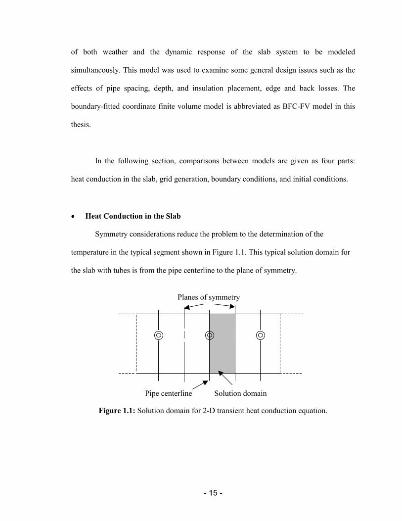
Symmetry considerations reduce the problem to the determination of the
temperature in the typical segment shown in Figure 1.1. This typical solution domain for
the slab with tubes is from the pipe centerline to the plane of symmetry.
Planes of symmetry
Solution domain Pipe centerline
Figure 1.1: Solution domain for 2-D transient heat conduction equation.
- 15 -
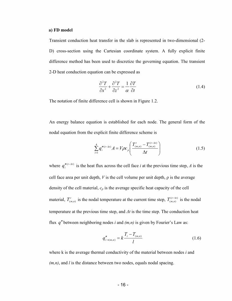
a) FD model
Transient conduction heat transfer in the slab is represented in two-dimensional (2-
D) cross-section using the Cartesian coordinate system. A fully explicit finite
difference method has been used to discretize the governing equation. The transient
2-D heat conduction equation can be expressed as
tT
zT
xT
�
��
�
��
�
�
�
12
2
2
2
(1.4)
The notation of finite difference cell is shown in Figure 1.2.
An energy balance equation is established for each node. The general form of the
nodal equation from the explicit finite difference scheme is
��
�
���
�
�
�
�
��
�
��
�tTT
cVAqtt
nmt
nmp
i
tti
)(),(),(4
1
)(� (1.5)
where is the heat flux across the cell face i at the previous time step, A is the
cell face area per unit depth, V is the cell volume per unit depth, ρ is the average
density of the cell material, c
)( ttiq ����
tnm ),(
��
p is the average specific heat capacity of the cell
material, T is the nodal temperature at the current time step, T is the nodal
temperature at the previous time step, and ∆t is the time step. The conduction heat
flux between neighboring nodes i and (m,n) is given by Fourier’s Law as:
)(),(tt
nm��
q
lTT
kq nminmi
),(),(
����
� (1.6)
where k is the average thermal conductivity of the material between nodes i and
(m,n), and l is the distance between two nodes, equals nodal spacing.
- 16 -
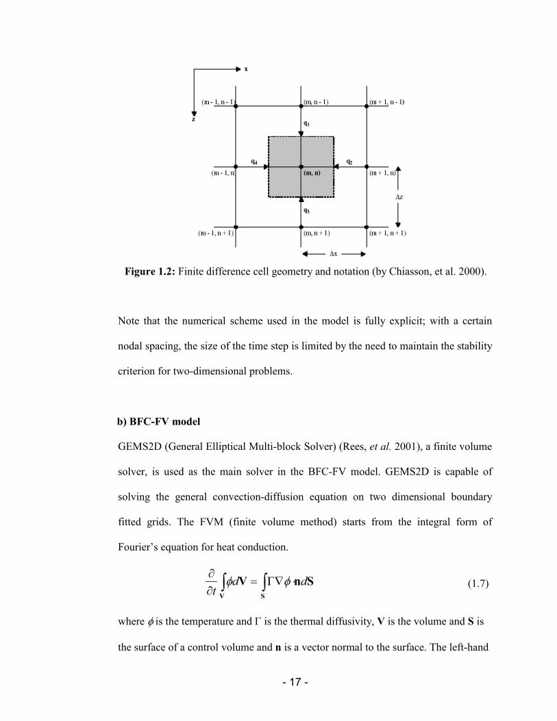
Figure 1.2: Finite difference cell geometry and notation (by Chiasson, et al. 2000).
Note that the numerical scheme used in the model is fully explicit; with a certain
nodal spacing, the size of the time step is limited by the need to maintain the stability
criterion for two-dimensional problems.
b) BFC-FV model
GEMS2D (General Elliptical Multi-block Solver) (Rees, et al. 2001), a finite volume
solver, is used as the main solver in the BFC-FV model. GEMS2D is capable of
solving the general convection-diffusion equation on two dimensional boundary
fitted grids. The FVM (finite volume method) starts from the integral form of
Fourier’s equation for heat conduction.
SnVSV
ddt �� �����
��� (1.7)
where � is the temperature and � is the thermal diffusivity, V is the volume and S is
the surface of a control volume and n is a vector normal to the surface. The left-hand
- 17 -
term of the equation is the temporal term and the right-hand term represents the
diffusion fluxes. A physical space approach for dealing with complex geometries can
be derived from the vector form of the equation above.
A second order approximation is to assume that the value of the variable on a
particular face is well represented by the value at the centroid of the cell face. The
diffusion flux at the east face of a cell can written as:
(1.8) eeD
e SdFe
)( nSnS
�������� � ��
where Se is the area of the east face.
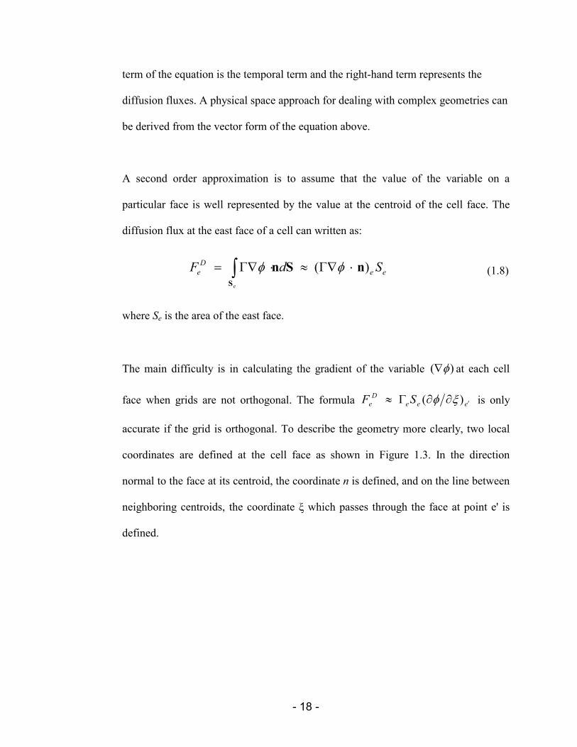
The main difficulty is in calculating the gradient of the variable ( at each cell
face when grids are not orthogonal. The formula
)��
eeeD
e SF�
�� )( �� �� is only
accurate if the grid is orthogonal. To describe the geometry more clearly, two local
coordinates are defined at the cell face as shown in Figure 1.3. In the direction
normal to the face at its centroid, the coordinate n is defined, and on the line between
neighboring centroids, the coordinate ξ which passes through the face at point e' is
defined.
- 18 -
P E
E’P’ e
ne
se
e’
s
n
w
n
x
x
y
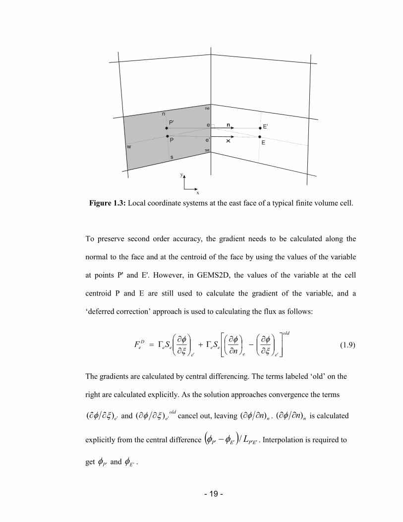
Figure 1.3: Local coordinate systems at the east face of a typical finite volume cell.
To preserve second order accuracy, the gradient needs to be calculated along the
normal to the face and at the centroid of the face by using the values of the variable
at points P' and E'. However, in GEMS2D, the values of the variable at the cell
centroid P and E are still used to calculate the gradient of the variable, and a
‘deferred correction’ approach is used to calculating the flux as follows:
old
eeee
eee
De n
SSF���
�
���
����
�
�
��
�
�
�
����
�
�
�
��
���
��
�
� (1.9)
The gradients are calculated by central differencing. The terms labeled ‘old’ on the
right are calculated explicitly. As the solution approaches convergence the terms
e��� )( �� and olde��� )��( cancel out, leaving nn)( ��� . nn)���( is calculated
explicitly from the central difference . Interpolation is required to
get � and � .
� � EPEP L����
� /��
P� E �
- 19 -
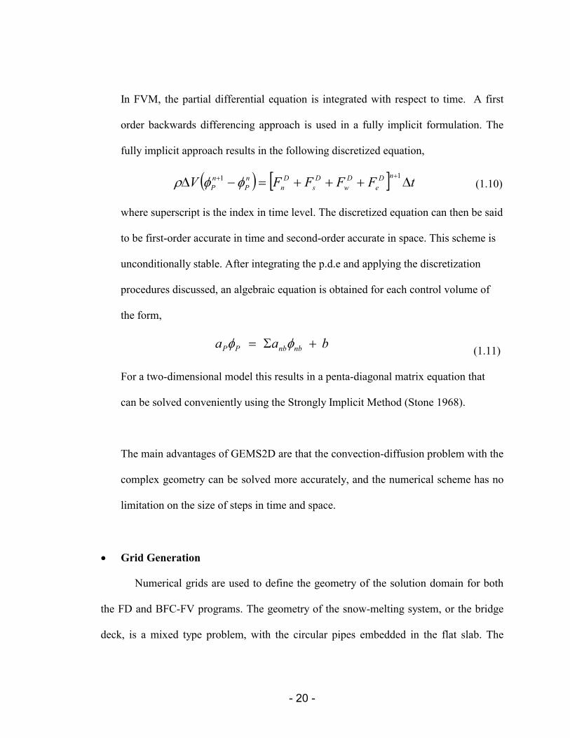
In FVM, the partial differential equation is integrated with respect to time. A first
order backwards differencing approach is used in a fully implicit formulation. The
fully implicit approach results in the following discretized equation,
(1.10) � � � tFFFFV nDe
Dw
Ds
Dn
nP
nP �������
��
11 ��� �
where superscript is the index in time level. The discretized equation can then be said
to be first-order accurate in time and second-order accurate in space. This scheme is
unconditionally stable. After integrating the p.d.e and applying the discretization
procedures discussed, an algebraic equation is obtained for each control volume of
the form,
baa nbnbPP ��� �� (1.11)
For a two-dimensional model this results in a penta-diagonal matrix equation that
can be solved conveniently using the Strongly Implicit Method (Stone 1968).
The main advantages of GEMS2D are that the convection-diffusion problem with the
complex geometry can be solved more accurately, and the numerical scheme has no
limitation on the size of steps in time and space.
�� Grid Generation
Numerical grids are used to define the geometry of the solution domain for both
the FD and BFC-FV programs. The geometry of the snow-melting system, or the bridge
deck, is a mixed type problem, with the circular pipes embedded in the flat slab. The
- 20 -
models use different coordinate systems to represent the geometry. The FD model uses a
rectangular coordinate system, while the 1090 model uses a boundary fitted approach.
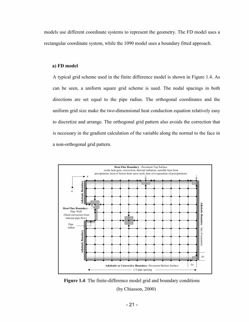
a) FD model
A typical grid scheme used in the finite difference model is shown in Figure 1.4. As
can be seen, a uniform square grid scheme is used. The nodal spacings in both
directions are set equal to the pipe radius. The orthogonal coordinates and the
uniform grid size make the two-dimensional heat conduction equation relatively easy
to discretize and arrange. The orthogonal grid pattern also avoids the correction that
is necessary in the gradient calculation of the variable along the normal to the face in
a non-orthogonal grid pattern.
1/2 pipe spacing
�z
��xAdiabatic or Convective Boundary- Pavement Bottom Surface
Adiabatic Boundary - line of sym
metry
Adi
abat
ic B
ound
ary
Adi
abat
ic B
ound
ary
Heat Flux Boundary - Pavement Top Surface (solar heat gain, convection, thermal radiation, sensible heat from
precipitation, heat of fusion from snow melt, heat of evaporation of precipitation)
Heat Flux Boundary -Pipe Wall
(fluid convection frominternal pipe flow)
Pipe radius
x
z
Figure 1.4: The finite-difference model grid and boundary conditions
(by Chiasson, 2000)
- 21 -
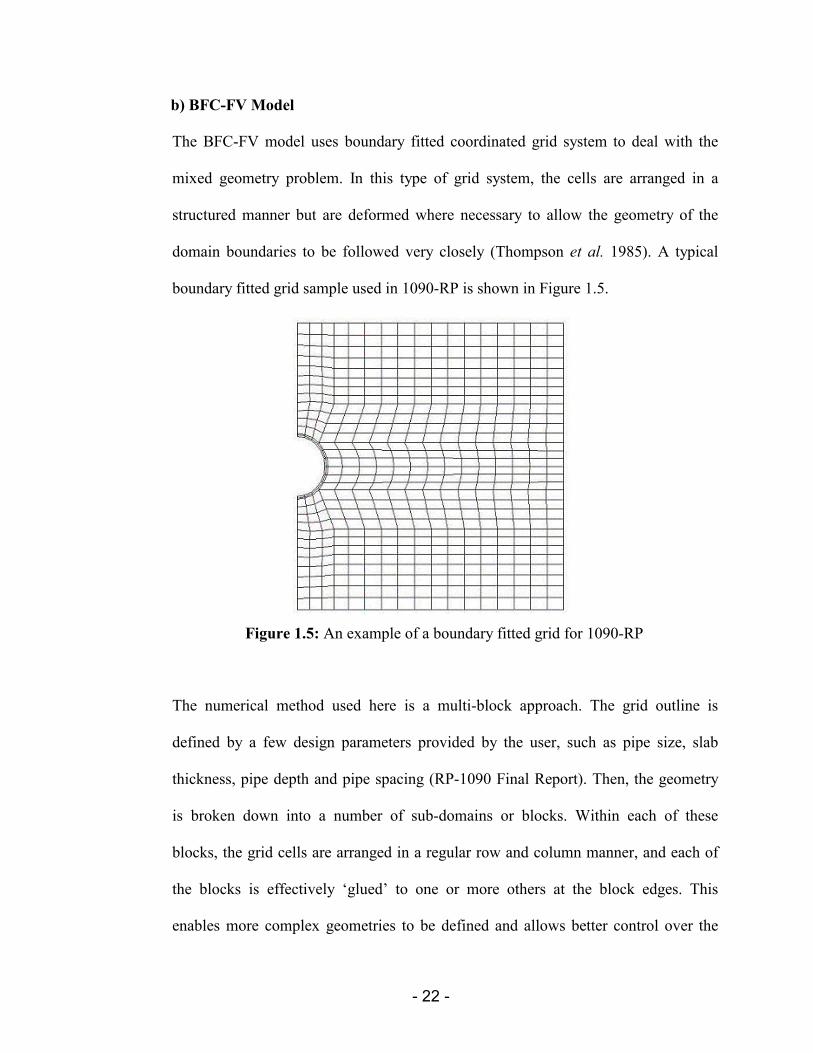
b) BFC-FV Model
The BFC-FV model uses boundary fitted coordinated grid system to deal with the
mixed geometry problem. In this type of grid system, the cells are arranged in a
structured manner but are deformed where necessary to allow the geometry of the
domain boundaries to be followed very closely (Thompson et al. 1985). A typical
boundary fitted grid sample used in 1090-RP is shown in Figure 1.5.
Figure 1.5: An example of a boundary fitted grid for 1090-RP
The numerical method used here is a multi-block approach. The grid outline is
defined by a few design parameters provided by the user, such as pipe size, slab
thickness, pipe depth and pipe spacing (RP-1090 Final Report). Then, the geometry
is broken down into a number of sub-domains or blocks. Within each of these
blocks, the grid cells are arranged in a regular row and column manner, and each of
the blocks is effectively ‘glued’ to one or more others at the block edges. This
enables more complex geometries to be defined and allows better control over the
- 22 -

grid cell distribution. A four-block grid definition of the slab containing a pipe is
show in Figure 1.6. Tests show that this four-block definition gives better control
over grid spacing and orthogonality than the definitions with fewer blocks.
Blo
ck 3
B
lock
2
Block 4
Block 1
Figure 1.6: Four-block definition of the slab containing a pipe.
Grid quality is determined by smoothness, cell aspect ratio and orthogonality. A
satisfactory grid quality is achieved by controlling the number of cells and the
distribution of nodes along each edge. A procedure was developed for ASHRAE
1090 RP for this purpose. The main criteria are summarized as follows.
1) In general, 25 edges and 4 blocks are necessary to specify the grid represent
the pipe and single pavement layer.
2) Additional pavement layers are taken as whole blocks.
3) It’s desirable to increase cell density towards the pipe both horizontally and
vertically. This is controlled by specifying different cell distribution functions
at the block edges.
4) The cell size should change gradually.
- 23 -
The advantage of the boundary fitted grids is that the geometry and pipe-wall
boundary condition can be represented more exactly. A simple algebraic grid
generation algorithm (Gordon and Hall 1973) is applied to calculate the cell vertex
positions in each block from a description of the geometry boundaries. This grid
information then is supplied to the main solver of the model.
�� Boundary Conditions
The main difficulty in boundary conditions is how to model the transient effect of
weather conditions on the top surface. The following paragraphs introduce the boundary
conditions applied to the FD model and BFC-FV model. Compared to the previous
models that apply the relationships (equation (1.1a-1.1f)) given by Chapman (1952) at the
upper boundary, the FD model is a great improvement in that it considers convective and
radiant losses occurred at the upper surface separately, hence, the effect of different
atmospheric factors, such as cloudiness and sky temperature, can be investigated more
accurately. The BFC-FV model presents a more detailed top boundary condition model.
It’s capable of giving a detailed analysis of the mass transfer among snow, ice, slush, etc.
For the boundary at the pipewall, the BFC-FV model uses a boundary-fitted grid
scheme to deal with the mixed geometry problem, while the FD model uses the square
grid to approximate the heat transfer area of the pipewall.
- 24 -
a) FD model
The boundary conditions are flux-type (Neumann boundary condition). The
temperature at each boundary node is given by the energy balance equation at that
node.
Boundary conditions at the top and bottom surface
The bottom surface is treated either as an insulated surface or as a surface exposed to
convective and radiant conditions. The top boundary condition is treated as flux-type
(Neumann boundary condition). The environmental interactions on the top surface
include the effects of solar radiation heat gain, long-wave radiation heat transfer,
convection heat transfer to the atmosphere, sensible heat transfer to snow, heat of
fusion required to melt snow, and heat of evaporation lost to evaporating rain or
melted snow. In the following paragraphs, a brief introduction to the first three flux
terms is given. This is followed by a more detailed introduction on the last three flux
terms.
Solar radiation heat gain is the net solar radiation absorbed by the slab surface, and is
decided by the absorptivity of the slab material, solar radiation incident on the slab
surface and the cosine of the incident angle. The long-wave radiation heat transfer at
each surface node is determined by the emissivity of the slab material, the nodal
temperature, and the temperature of the surroundings. The convection heat flux at
each pavement surface node is computed by the dry-bulb air temperature and the
nodal temperature, and the convective heat transfer coefficient is taken as the
- 25 -
maximum of the free convection coefficient and the forced convection coefficient
which can be found in Incropera and DeWitt (1996).
Heat flux due to the rain and snow includes both sensible and latent effects. Sensible
heat flux is decided by precipitation and temperature difference between the dry-bulb
air temperature and the nodal temperature. Latent heat flux is considered only if the
air temperature or the slab surface temperature is above 33oF (0.55oC). There are two
kinds of latent heat flux that may be considered. One is the latent heat of
vaporization, and the other is the heat flux due to melting snow and ice. Both of them
relate to the mass transfer occurred on the surface. One main assumption made for
mass transfer is: accumulation of rain is not considered; rainfall is assumed to drain
instantaneously from the pavement surface, forming a thin film from which
evaporation occurs.
This model uses the j-factor analogy to compute the mass flux of evaporating water
at each pavement surface node ( ): wm ���
� �� �1,mairdw wwhm ����� (1.12)
where hd is the mass transfer coefficient, wair is the humidity ratio of the ambient air,
and w(m,1) represents the humidity ratio of saturated air at the surface node. The mass
transfer coefficient (hd) is defined using the Chilton-Colburn analogy:
3/2Lechh
p
cd � (1.13)
- 26 -
where hc is the convection coefficient, cp is the specific heat capacity of the air
evaluated at the pavement node - air film temperature, and Le is the Lewis number.
The heat flux due to evaporation ( ) is then given by: nevaporatioq ��
q (1.14) wfgnevaporatio mh ����� �
where hfg is the latent heat of vaporization.
The heat flux due to melting snow and ice is determined using a mass balance on
freezing precipitation that has accumulated at the pavement surface. The sum of the
rainfall rate and the snowfall rate are taken as the accumulation of the ice when the
air temperature or the slab surface temperature is below 33oF. The mass flux of water
due to melting ice ( ) at the pavement surface is then given by: icemeltedm ���
if
iceconductionnevaporatiosensiblesnowrainconvectionthermalsolaricemelted h
qqqqqqm ,_, �����������������
���� (1.15)
where is the conduction heat flux from the pavement surface into the ice
layer and h
iceconductionq ,��
convectionq ��
if is the latent heat of fusion of water. The other heat flux terms are solar
radiation heat gain , long-wave radiation heat transfer , convection heat
transfer to the atmosphere, sensible heat transfer to snow, and
heat of evaporation lost to evaporating rain or melted snow. The numerator
in equation (1.16) is the heat flux into each pavement surface node ( q ):
solarq ��
evaporatioq ��
thermalq ��
snowrain _,� sensibleq�
� ,m��
n
�1
(1.16) � � iceconductionnevaporatiosensiblesnowrainconvectionthermalsolarm qqqqqqq ,_,1, ���������������������
- 27 -
The thickness of the ice layer at the end of the time step (lice,new) is given by:
tmmllice
icemeltedwoldicenewice ���
�
����
� �����
�
��
,, . (1.17)
Boundary conditions at the pipe wall
The boundaries of the left and right hand of the solution domain are adiabatic, except
the boundaries of the pipe surface nodes. Heat fluxes at these nodes are determined
by the heat transfer due to heat exchange fluid as equation (1.18).
� �� �nmfluidpipefluid TTUq ,���� (1.18)
where the average fluid temperature Tfluid is used to characterize the fluid. Upipe is the
overall heat transfer coefficient for the pipe and expressed as:
pipepipe
pipe
kl
h�
� 11U (1.19)
where hpipe is the convection coefficient due to fluid flow through the pipe, kpipe is the
thermal conductivity of the pipe material, and l is the wall thickness of the pipe.
Since the outlet temperature at any current time step is not known, the outlet fluid
temperature is solved in an iterative manner. The iteration is considered converged
when the heat flux calculated by the resistance method is consistent with that
resulted from the overall energy balance calculation.
Boundary conditions implemented in the FD model have two main shortcomings.
The model can’t give the mass distribution of each phase on the surface nodes. In
- 28 -
this model, although snow is a porous medium, it is treated as an equivalent ice
layer, and it hasn’t considered the interactions among snow, slush, and ice. Thus, the
heat and mass transfer calculation for the surface is relatively rough. Approximating
the round geometry at the source location by square grids enlarges the actual heat
transfer area, and the model tends to over-predict the heat transfer rate occurring at
the boundary. As can be seen from Figure 1.4, the nodes labeled as pipe wall do not
represent the pipe geometry well. They are actually nodes in the concrete that have
direct contact with the outer pipe wall. The square grid scheme used in the FD model
doesn’t include the pipe in the solution domain. In addition to causing steady state
error, it may cause error early on in the transient response.
b) BFC-FV Model
Boundary conditions at the pipe wall
The boundary condition at the pipe wall is specified in a relatively simple form in the
BFC-FV model. Users can specify either the constant heat flux at the pipe wall as the
boundary condition, or the average fluid temperature and Reynolds number.
Boundary conditions at the bottom surface
The bottom surface is treated either as a surface exposed to convective and radiant
conditions, or as a surface in contact with the ground. In modeling an exposed
condition where the slab is not ground coupled, such as in a bridge or ramp, a simple
boundary condition is applied. In this case the surface is assumed dry and exposed to
- 29 -
the wind, but not exposed to the sky. Convective and long-wave radiant heat transfer
to surroundings is considered.
In the case that soil is considered beneath the slab, users can decide whether to
include an insulation layer at the slab bottom, and set the ground temperature of the
very lower surface of the ground if necessary. Otherwise, the BFC-FV model would
specify a ground temperature as the bottom boundary condition for the model. A
one-dimensional analytical solution developed by Kusuda and Achenbach (1965) is
applied to calculate the annual temperature cycle at the surface of the earth. It makes
use of a simple harmonic function based on simplified conduction theory, where it is
assumed that earth is a semi-infinite homogeneous heat-conducting medium, with
constant thermal diffusivity. The harmonic function provided in the paper is
expressed as:
��
�
�
��
�
���
��
����
����
���
����
��
POxDTT
BOeAtx
DT ����
2cos (1.20)
where,
x = downward distance from the earth’s surface, ft [m],
t = earth temperature, oF [oC],
θ = time coordinate which is taken as zero on January 1st,
T = period of the temperature cycle (8766 hour),
A = annual average earth temperature oF [oC],
BO = earth surface temperature amplitude, radians,
PO = earth surface temperature phase angle, radians,
- 30 -
D = thermal diffusivity of the earth ft2/hr [m2/hr].
The paper provides information regarding A, BO, PO, and D for many locations
around U.S. However, for locations for which the values of A, BO, PO, and D are not
available, the values corresponding to the nearest location available in Kusuda and
Anchebach (1965) have been used.
Boundary conditions at the top surface
The BFC-FV model includes a boundary condition model to present more detailed
temperature and mass distributions on the slab upper surface. The boundary
condition model is a collection of heat and mass sub models for each type of surface
condition that may occur. The approach to this aspect of the modeling task has been
to treat the snow layer as quasi one-dimensional. Each surface node on the two-
dimensional slab is coupled to an instance of the surface boundary condition model.
The function of the boundary condition model is to identify a number of possible
surface conditions and apply the sub models to calculate the temperature and mass
distribution at local nodes. Which model is applied to calculate the surface condition
at the end of current time step of the simulation is decided based on the conditions at
the end of the last time step, the current type of precipitation, and the current surface
temperature.
There are a variety of surface conditions that may occur. The slab may be dry,
covered in “slush”, or solid ice. The slab may be wet not only because of rain but
also at the final stages of melting. The surface condition is determined from the
surface temperature and the mass of ice and water on each cell. A summary of the
- 31 -
possible current conditions, and the possible conditions at the end of the time step,
are given in Table 1.1. The surface conditions that have been considered are defined
as follows:
Dry: The surface is free of liquid and ice. The surface temperature may be above
or below freezing.
Wet: The surface is above freezing and has some liquid retained on it, but no ice.
Dry Snow: The snow has freshly fallen snow on it but no liquid. The snow can be
regarded as a porous matrix of ice. The surface temperature is below freezing so
that snow is not currently being melted.
Slush: The surface contains ice in the form of snow crystals that are fully
saturated with water. Water penetrates the ice matrix to the upper surface. The
surface temperature is at the freezing point.
Snow and Slush: The surface contains snow that is partly melted. The lower part
of the snow is saturated with water and the upper is as dry snow. This is the
general melting snow condition and the surface temperature is at freezing point.
Solid Ice: The ice on the surface is in solid form rather than porous like snow.
The surface temperature must be below freezing.
Solid Ice and water: The surface consists of solid ice and water. This can occur
when rain falls on solid ice or when the solid ice is being melted. Melting can be
from below or above. The surface temperature is at freezing.
- 32 -
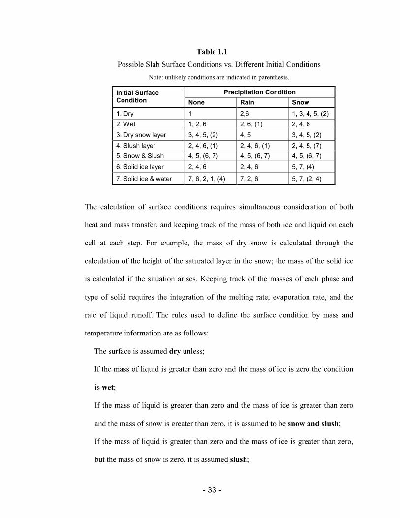
Table 1.1 Possible Slab Surface Conditions vs. Different Initial Conditions
Note: unlikely conditions are indicated in parenthesis.
Precipitation Condition Initial Surface Condition None Rain Snow 1. Dry 1 2,6 1, 3, 4, 5, (2) 2. Wet 1, 2, 6 2, 6, (1) 2, 4, 6 3. Dry snow layer 3, 4, 5, (2) 4, 5 3, 4, 5, (2) 4. Slush layer 2, 4, 6, (1) 2, 4, 6, (1) 2, 4, 5, (7) 5. Snow & Slush 4, 5, (6, 7) 4, 5, (6, 7) 4, 5, (6, 7) 6. Solid ice layer 2, 4, 6 2, 4, 6 5, 7, (4)
7. Solid ice & water 7, 6, 2, 1, (4) 7, 2, 6 5, 7, (2, 4)
The calculation of surface conditions requires simultaneous consideration of both
heat and mass transfer, and keeping track of the mass of both ice and liquid on each
cell at each step. For example, the mass of dry snow is calculated through the
calculation of the height of the saturated layer in the snow; the mass of the solid ice
is calculated if the situation arises. Keeping track of the masses of each phase and
type of solid requires the integration of the melting rate, evaporation rate, and the
rate of liquid runoff. The rules used to define the surface condition by mass and
temperature information are as follows:
The surface is assumed dry unless;
If the mass of liquid is greater than zero and the mass of ice is zero the condition
is wet;
If the mass of liquid is greater than zero and the mass of ice is greater than zero
and the mass of snow is greater than zero, it is assumed to be snow and slush;
If the mass of liquid is greater than zero and the mass of ice is greater than zero,
but the mass of snow is zero, it is assumed slush;
- 33 -
If the mass of liquid is zero and the mass of ice is greater than zero and the mass
of snow is greater than zero, it is assumed to be dry snow;
If the mass of liquid is zero and the mass of solid ice is greater than zero, but the
mass of snow is zero, it is assumed to be solid ice;
If the mass of liquid is greater than zero and the mass of solid ice is greater than
zero, but the mass of snow is zero, it is assumed to be solid ice and water.
The boundary conditions of the finite volume solver can be specified as fixed
temperature, fixed flux, or a linear mixed condition. The boundary conditions are
highly non-linear as phase change occurs at the boundary. It is necessary to have a
much more complicated model for the calculation of the slab surface temperature
that is more loosely coupled to the finite volume solver.
The finite volume solver (GEMS2D) is coupled to the boundary condition model by
passing surface temperature information and heat flux information between the two
models. Because the temperature becomes fixed at the point of melting, it is
necessary that the finite volume solver pass the surface flux it has calculated to the
boundary condition model. The boundary condition model then calculates the surface
temperature and the mass condition under this surface flux input. The new surface
temperature is, in turn, passed back to the finite volume solver. This iterative process
is considered converged when the heat flux calculated by the finite volume solver
becomes consistent with the surface temperature calculated by the boundary
condition model.
- 34 -
There are seven pairs of sub models corresponding to seven types of surface
conditions that may occur as tabulated in Table 1.1. For brevity, only the melting
snow model is discussed in detail.
The melting snow model
First, conceptually the snow during the melting process is considered as a layer of
“dry” snow (ice crystals with no liquid water), and a layer of saturated snow (slush)
adjacent to the slab surface. Both the snow layer and the saturated layer may be
considered as porous media. The dry snow layer has air in the void space between
the snow crystals, and the saturated layer has water in the void space between the
snow crystals.
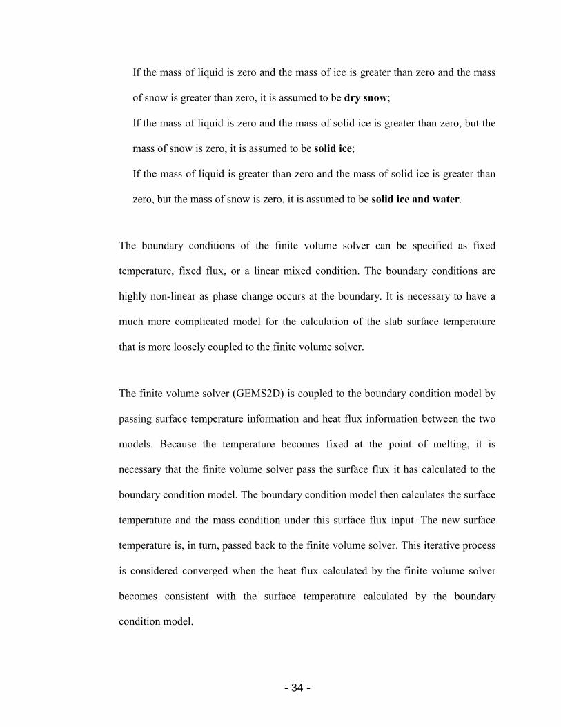
The mass transfers of interest to or from the snow layer are shown in Figure 1.7. The
snowfall rate is determined from weather data. Snowmelt rates are determined based
on an energy balance, to be discussed below. Sublimation isn’t included in the
model, as it seemed an insignificant effect. It is also assumed that as melting occurs
the slush-snow line will move so that previously dry snow will become saturated
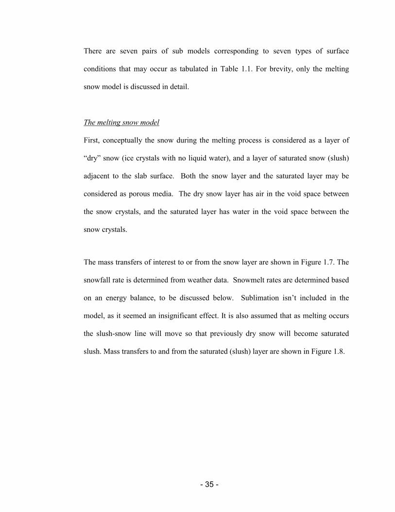
slush. Mass transfers to and from the saturated (slush) layer are shown in Figure 1.8.
- 35 -
Slab
Slush/liquid layer
Snow layer
Atmosphere
Snowfall Sublimation
Snow transferred to slush layer
Figure 1.7: Mass transfer to/from the snow layer.
Slab
Slush/liquid layer
Snow layer
Atmosphere
RainfallEvaporation
Snow transferred to slush layer
Runoff Snowmelt
Figure 1.8: Mass transfer to/from the slush layer
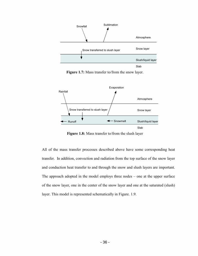
All of the mass transfer processes described above have some corresponding heat
transfer. In addition, convection and radiation from the top surface of the snow layer
and conduction heat transfer to and through the snow and slush layers are important.
The approach adopted in the model employs three nodes – one at the upper surface
of the snow layer, one in the center of the snow layer and one at the saturated (slush)
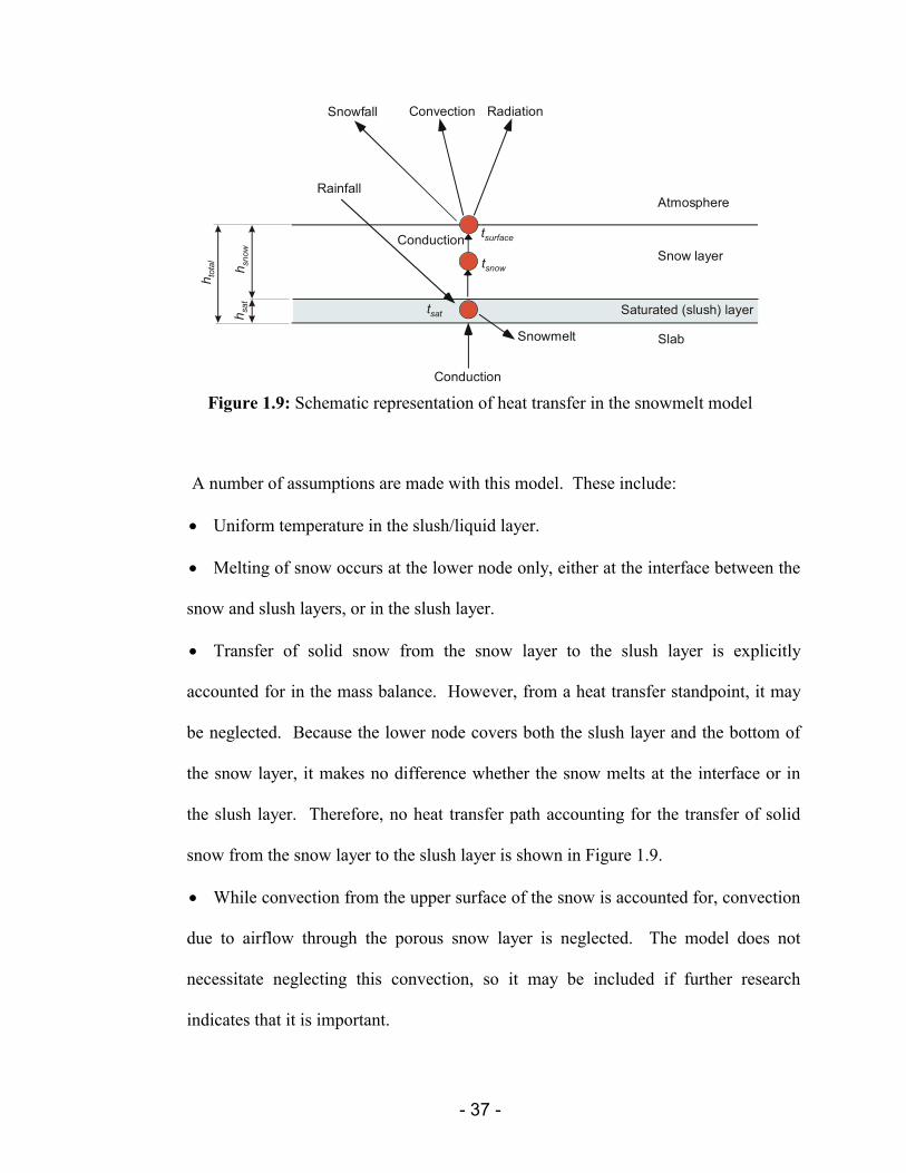
layer. This model is represented schematically in Figure. 1.9.
- 36 -
Slab
Snow layer
AtmosphereRainfall
Snowmelt
Convection Radiation
Conduction
Conduction
Snowfall
tsurface
tsnow
tsat Saturated (slush) layerh sat
h snow
h total
Figure 1.9: Schematic representation of heat transfer in the snowmelt model
A number of assumptions are made with this model. These include:
�� Uniform temperature in the slush/liquid layer.
�� Melting of snow occurs at the lower node only, either at the interface between the
snow and slush layers, or in the slush layer.
�� Transfer of solid snow from the snow layer to the slush layer is explicitly
accounted for in the mass balance. However, from a heat transfer standpoint, it may
be neglected. Because the lower node covers both the slush layer and the bottom of
the snow layer, it makes no difference whether the snow melts at the interface or in
the slush layer. Therefore, no heat transfer path accounting for the transfer of solid
snow from the snow layer to the slush layer is shown in Figure 1.9.
�� While convection from the upper surface of the snow is accounted for, convection
due to airflow through the porous snow layer is neglected. The model does not
necessitate neglecting this convection, so it may be included if further research
indicates that it is important.
- 37 -
�� Likewise, convection and evaporation from the slush layer are neglected (when
covered with a layer of dry snow).
�� Rainfall occurring after a snow layer has formed is accounted for directly only at
the saturated layer.
�� The snow melting process is treated as a quasi-one-dimensional process.
The model is formed by five primary equations – a mass balance for the solid ice, a
mass balance for liquid water, and a heat balance on each node. The mass balance on
the ice is given by:
meltsnowfallice mm
ddm
�� �������
(1.21)
where,
icem = the mass of snow per unit area in the snow layer, lbm/ft2 [kg/m2],
θ = the time, hr or s
snowfallm� �� = the snowfall rate in mass per unit area, lbm/(hr-ft2) [kg/s-m2],
meltm� �� = mass rate of snow that is transferred to the slush in solid form, lbm/(hr-ft2) or
[kg/s-m2].
The mass balance on the liquid is given by:
runoffrainmeltl mmm
ddm
��� ����������
(1.22)
lm = the mass of liquid water per unit area in the slush layer, lbm/ft2 [kg/m2],
rainm� �� = the rainfall rate in mass per unit area, lbm/(hr-ft2) [kg/s-m2],
- 38 -
meltm� �� = the snowmelt rate in mass per unit area, lbm/(hr-ft2) [kg/s-m2],
runoffm� �� = the rate of runoff in mass per unit area, lbm/(hr-ft2) [kg/s-m2].
A simple heuristic approach has been taken to estimate the amount of runoff. In
order to approximate the effect of water being retained in the snow due to capillary
action, the runoff is limited to 10% of the melt rate until the saturated layer is 2
inches thick. The runoff rate is increased to the melt rate after this point in order to
prevent more water being retained.
In order to calculate the heat balances on the snow and saturated layers it is
necessary to work out the total mass of these two layers. This can be done by
assuming an effective porosity (or relative density) and calculating the thickness of
these layers. The total height of the snow and slush layers can be found from the
mass of ice by:
)1( effice
icetotal n
mh�
�
� (1.23)
where
htotal = the total thickness of the snow and saturated layers, ft [m],
neff = the effective porosity of the ice matrix (applies to both layers), dimensionless,
ρice = the density of ice, lbm/ft3 [kg/m3].
The height of the saturated layer can be calculated from the mass of liquid,
effl
lsat n
mh�
� (1.24)
- 39 -
The height of the snow layer can be found by subtracting, hsnow=htotal - hsat. Having
worked out the height of the respective layers their mass of the dry snow layer can be
found:
)1( effsnowicesnow nhm �� � (1.25)
The mass balance equations are coupled to the energy balance equations by the melt
rate. The energy balance on the snow layer is given conceptually as:
radiationconvectionsnowfallsnowconductionsnow
psnow qqqqd
dtcm ������������ ,�
(1.26)
However, each of the various terms must be defined in additional detail. The
conduction heat flux from the slush layer to the snow layer is given by:
)(5.0, snowslush
snow
snowsnowconduction tt
hkq ���� (1.27)
where
ksnow= the thermal conductivity of the snow. Btu/(hr-ft-F) [W/m-K],
tsat = the temperature of the slush layer, oF [oC],
tsnow = the temperature of the snow node, oF [oC],
The heat flux due to snowfall is given as:
)(, asnowicepsnowfallsnowfall ttcmq ������ � (1.28)
The convective heat flux is given by:
- 40 -
)( asurfacecconvection tthq ���� (1.29)
The radiative heat flux is given by:
)( 44MRsurfacesradiation TTq ���� �� (1.30)
surfaceT is the absolute temperature of the slab surface, and T is the absolute mean
radiant temperature of surroundings. Under snowfall condition, surroundings are
approximately at the ambient air temperature. When there is no snow precipitation,
the mean radiant temperature is approximated by the following equation:
MR
� �� 4/14
4 1 scclearskysccloudMR FTFTT ��� � (1.30-a)
where, is the fraction of the radiation exchange that takes between slab and
clouds, T is the absolute temperature of clouds, and T is the absolute
temperature of clear sky.
scF
cloud clearsky
The snow surface temperature is found from a heat balance on the surface node:
)(5.0 radiationconvection
snow
snowsnowsurface qq
hktt ������� (1.31)
The surface temperature has to be determined iteratively for the radiation and heat
balance calculation at each node. The slush layer is presumed in thermodynamic
equilibrium so that the temperature of the slush is uniform at melting point. Then, the
energy balance is given by:
(1.32) snowconductionrainfallslabconductionifmelt qqqhm ,, ������������
- 41 -

Assuming rainwater will be at the air temperature, the heat flux due to rainfall is
given by:
)(, slushawaterprainfallrainfall ttcmq ������ � (1.33)
The mean radiant temperature and convection coefficient are calculated in the same
manner as in Ramsey et al. (1999a).
The boundary condition model of the BFC-FV model also has disadvantages. The
heat flux from solar radiation is not considered. This may be acceptable under
design snowfall weather conditions. But to determine actual system performance,
solar radiation needs to be considered. The price for the detailed treatment of the
mass and temperature distribution on the surface is the computing time. Much time
has been spent on the iteration between the main solver and the boundary condition
model.
As noted in the section of grid generation, the pipe is included in the solution
domain. The boundary conditions at the pipe nodes can be specified as usual types,
fixed temperature, fixed flux, or a linear mixed condition. Temperatures at these
nodes are solved by the main solver with the other nodal temperatures inside the
domain.
�� Initial Conditions
In a transient calculation, the initial conditions applied to the calculation can be
just as significant as the boundary conditions. For the FD model, the initialization is
- 42 -
relatively simple- all the nodal temperatures are set to the dry bulb air temperature at the
simulation starting time, and as described in the previous section, the bottom is set
adiabatic. In the BFC-FV model, the initial slab and the ground temperatures have been
initialized according to location and weather conditions.
In order to take account of ground heat transfer, it is necessary not only to specify
the temperature at the bottom boundary (the lower surface of the ground), but also to
calculate the temperature profile through the calculation domain. This temperature profile
is driven by the ground temperature and the weather prior to the storm event. Therefore,
the BFC-FV model extends the period of simulation to include many more hours before
the start of the storm. The approach taken involves using a one-dimensional model of
slab and ground. The ground temperature is specified at the lower boundary, and a two-
week period is simulated. To initialize the two-dimensional model, the final temperature
profile calculated using the one-dimensional model is taken and used to define the initial
temperatures (according to cell depth) over the 2D grid. For each storm, the two-
dimensional calculation is made of six hours of weather data before the start of any snow
precipitation.
1.2.2.3 Transfer Function Method
Transient heat transfer in the two-dimensional slab can be solved numerically in a
variety of ways. The models mentioned above use numerical methods- finite difference
and finite volume. However, these methods have drawbacks in computational efficiency
because a large number of cells have been used to ensure accuracy. Another possible
- 43 -
modeling method is a time series method. Generally, this method requires less time in
computing. Several of the detailed building energy analysis programs such as EnergyPlus
use a time series solution to transient heat conduction in building wall. The most basic
time series solution is the response factor equation, which relates the flux at one surface
of an element to an infinite series of temperature histories on both sides. The conduction
transfer formulation replaces the infinite series of temperatures with a finite number of
temperature and flux history terms.
The basic form of a conduction heat transfer function (CTF) solution without a
heat source or sink, giving heat flux at the inside surface, is shown as follows:
� ��� �
���
�
���������
M
m
k
mmtimmtom
M
mmtimti qFTYTXq
1 1,1,
11,, (1.34)
Where k is the order of the conduction transfer functions, M is a finite number defined by
the order of the conduction transfer functions, and X, Y, and F are the conduction function
coefficients. The equation relates the current heat flux at the interior surface via a linear,
algebraic equation to temperature and heat flux histories.
Strand (1995, 1997) developed and verified heat source transfer functions (QTFs)
for transient heat conduction with a source or sink. As with the CTFs, the QTFs can be
derived by a Laplace transform or a state space method while the heat source transmitted
to the slab is treated as a definable, variable input. The QTFs are in a similar form to the
CTFs as:
1
1,1
",
11,,
11,,
", ����
�
��
�
�
�
��
�
������
M
mmtsourcem
k
mmtim
M
mmtomk
M
mmtimkti qWqFTYTXq (1.35)
- 44 -
Where, X, Y, Z, F and W are the heat source transfer function coefficients. The heat
source history is taken into the consideration. The QTF method is described in more
detail in Chapter 3.
1.3. Thesis Objective and Scope
This study aims at modeling transient performance of the hydronic
heating/cooling system. The study is intended to achieve a better understanding of
systems to establish better design guidelines in future. The three main objectives of this
study can be summarized as follows:
1) Develop and implement a parametric study of snow-melting systems for
ASHRAE 1090-RP. Examine general design issues such as the effects of pipe
spacing, depth, insulation placement, and edge and back losses under the
transient weather conditions and system operations.
2) Develop a new heated bridge deck model based on the time series method
(QTFs).
3) Use the model to analyze the performance and behavior of actual bridge deck
heating systems.
Chapter 2 of this thesis addresses the first objective. The snow-melting model
developed for ASHRAE 1090-RP is used to simulate the transient response of the slab
during the storm event. A center zone is evaluated for 360 cases of various
configurations. The minimum heat fluxes that are required to achieve the specified free
area ratio are found for these cases. The back losses are examined. An edge zone is
- 45 -
studied with 180 cases of various configurations. The minimum fluxes found in the center
zone study are applied in the edge zone cases. The surface conditions achieved in the
edge zone are checked. The edge losses are examined.
Chapter 3 of this thesis addresses the second objective. The development and
validation of a bridge deck model based on the time series method is presented. The
simulation results are compared with the analytical solution and results from other
software.
Chapter 4 of this thesis addresses the third objective. The model based on the time
series method is applied to predict the performance of a hydronic bridge deck system
under real weather conditions. The heating mode and the recharge mode are examined.
Results are compared to experimental measurements.
Finally, Chapter 5 of this thesis summarizes the conclusions of the individual
studies.
- 46 -
2. Parametric Study of Snow-Melting System
2.1. Introduction
The transient behavior of snow-melting systems is caused by dynamic weather
conditions and intermittent system operation. The thermal mass in the system is quite
significant and introduces significant time lag into the system. The thermal history of the
system and the transient nature of the weather have been taken into account in this
chapter.
The work of this chapter has been performed as a part of the ASHRAE 1090-RP
(research project). The numerical method is based on the earlier contributions of the
project. This project is aimed at studying the significance of transient effects on the
snow-melting system performance. This chapter describes an investigation of the effects
of two phenomena on the transient snow-melting system behavior. One is back and edge
losses, and the other is transient design conditions and operation of the snow-melting
system. Two parametric studies are described. The studied parameters include pipe
spacing, pipe depth, pipe diameter, insulation level, soil conductivity, location, and storm.
The minimum pipe fluxes have been found to maintain either:
��A free area ratio of one, for all hours of the storm, except a number of hours
equivalent to the number of hours for which the steady-state 99% non-exceedance
conditions were exceeded (the concept of the steady-state 99% non-exceedance
condition is introduced below).
- 47 -
��Or, for the free area ratio of zero case, the minimum pipe flux was found that only
allowed the snow height to increase for a number of hours equivalent to the
number of hours for which the steady-state 99% non-exceedance conditions were
exceeded.
If input pipe flux is less than the minimum, the surface can’t achieve or maintain
the specified free area ratio. Some terminology is defined as follows.
�� A certain percentile steady-state load and non-exceedance conditions
The steady-state loads (according to the ASHRAE 926-RP calculation procedure) for
each location were calculated for 12 years of available data for a free area ratio of 1.0
or 0.0. Sorting of all the hours of data according to the size of load allows different
percentile loads to be found. For a given storm, the number of hours the steady-state
loads are above a particular percentile can be counted. There are four percentiles
conventionally considered, namely the 99, 95, 90, and 75 percentile.
The number of hours in the storm above the percentile of interest is probably a good
indication of the severity of the storm. The steady-state percentile non-exceedance
condition is that the steady-state loads of a given storm are below the specified
percentile.
�� Heat fluxes
Heat flux supplied to the pipe is called input heat flux or input flux. When specifying
the boundary condition at the pipe wall, input flux is in units of BTU/(hr per ft of
pipe). Heat flux at the upper surface of the slab is called surface flux. Heat flux at the
bottom surface of the slab is called back loss, and edge loss is the heat transfer
- 48 -
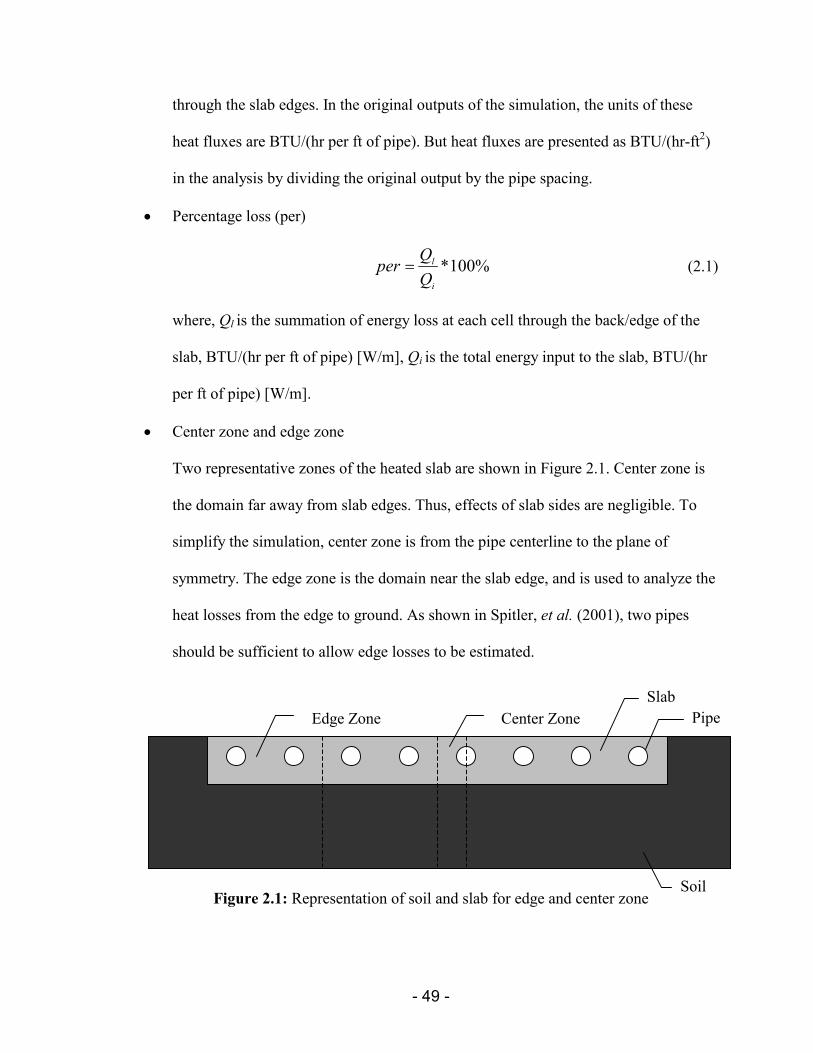
through the slab edges. In the original outputs of the simulation, the units of these
heat fluxes are BTU/(hr per ft of pipe). But heat fluxes are presented as BTU/(hr-ft2)
in the analysis by dividing the original output by the pipe spacing.
�� Percentage loss (per)
%100*i
l
per � (2.1)
where, Ql is the summation of energy loss at each cell through the back/edge of the
slab, BTU/(hr per ft of pipe) [W/m], Qi is the total energy input to the slab, BTU/(hr
per ft of pipe) [W/m].
�� Center zone and edge zone
Two representative zones of the heated slab are shown in Figure 2.1. Center zone is
the domain far away from slab edges. Thus, effects of slab sides are negligible. To
simplify the simulation, center zone is from the pipe centerline to the plane of
symmetry. The edge zone is the domain near the slab edge, and is used to analyze the
heat losses from the edge to ground. As shown in Spitler, et al. (2001), two pipes
should be sufficient to allow edge losses to be estimated.
Figure 2.1: Representation of soil and slab for edge and center zone Soil
Slab Pipe Edge Zone Center Zone
- 49 -

�� System operation
Based on the recommendations of the ASHRAE Project Monitoring Subcommittee,
idling isn’t considered in the study, as it is never or almost never utilized today.
�� Number of hours excluded
The number of hours where the performance is allowed to fall below the design
criterion is called the number of hours excluded in the parametric study.
2.2. Methodology of Parametric Study
The snow-melting model used in ASHRAE 1090-RP is the highly detailed two-
dimensional transient model (the BFC-FV model) described in Chapter 1. The model can
provide the temperature distribution of the slab and surroundings for the whole length of
the storm.
2.2.1. Organization and Methodology of Parametric Study
Current snow-melting system design procedures are based on conditions typical
of the center slab zone. Some snow coverage at the edge of the slab is likely to be
tolerated. Accordingly, edge losses and snow-melting performance at the edge of the slab
are based on design heat inputs found for center. So the first step is a large parametric
study in which the minimum fluxes for the center zones to maintain a specified free area
ratio are determined. The results enable us to determine the transient effect of the design
conditions/operations and back losses on the design loads. Then the same input heat
fluxes are supplied to the edge zone. This enables us to find the edge losses under these
conditions and the corresponding minimum free area ratio achieved.
- 50 -
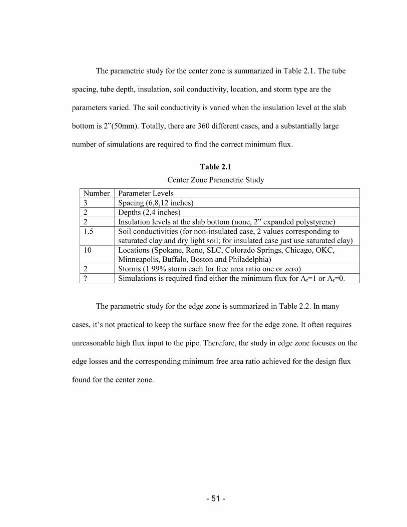
The parametric study for the center zone is summarized in Table 2.1. The tube
spacing, tube depth, insulation, soil conductivity, location, and storm type are the
parameters varied. The soil conductivity is varied when the insulation level at the slab
bottom is 2”(50mm). Totally, there are 360 different cases, and a substantially large
number of simulations are required to find the correct minimum flux.
Table 2.1 Center Zone Parametric Study
Number Parameter Levels 3 Spacing (6,8,12 inches) 2 Depths (2,4 inches) 2 Insulation levels at the slab bottom (none, 2” expanded polystyrene) 1.5 Soil conductivities (for non-insulated case, 2 values corresponding to
saturated clay and dry light soil; for insulated case just use saturated clay) 10 Locations (Spokane, Reno, SLC, Colorado Springs, Chicago, OKC,
Minneapolis, Buffalo, Boston and Philadelphia) 2 Storms (1 99% storm each for free area ratio one or zero) ? Simulations is required find either the minimum flux for Ar=1 or Ar=0.
The parametric study for the edge zone is summarized in Table 2.2. In many
cases, it’s not practical to keep the surface snow free for the edge zone. It often requires
unreasonable high flux input to the pipe. Therefore, the study in edge zone focuses on the
edge losses and the corresponding minimum free area ratio achieved for the design flux
found for the center zone.
- 51 -

Table 2.2 Edge Zone Parametric Study
Number Parameter Levels 3 Spacing (6,8,12 inches) 2 Depths (2,4 inches) 2 Insulation levels at the slab bottom (none, 2” expanded polystyrene) 1.5 Soil conductivities (for non-insulated case, 2 values corresponding to
saturated clay and dry light soil; for insulated case just use saturated clay)
10 Locations (Spokane, Reno, SLC, Colorado Springs, Chicago, OKC, Minneapolis, Buffalo, Boston and Philadelphia)
2 Storms (1 99% storm each for free area ratio one or zero) 1 Heat flux (the same as the minimum flux found by center zone study).
2.2.2. Methodology of Center Zone Parametric Study
The center zone parametric study investigates the effect of the transient design
condition/operation and back losses on the design loads and compare these transient
design loads. As shown in Table 2.1, there are 360 cases to study and a large number of
simulations are needed for finding the minimum flux. The methodology for the center
zone study may be described in three parts,
��development of minimum flux search algorithm,
��batch processing,
��post-processing of data.
Search Algorithm for Minimum Flux
The search algorithm automatically and iteratively runs the simulation to find the
minimum flux within some tolerance. A flow chart for the search algorithm is shown in
Figure 2.2.
- 52 -
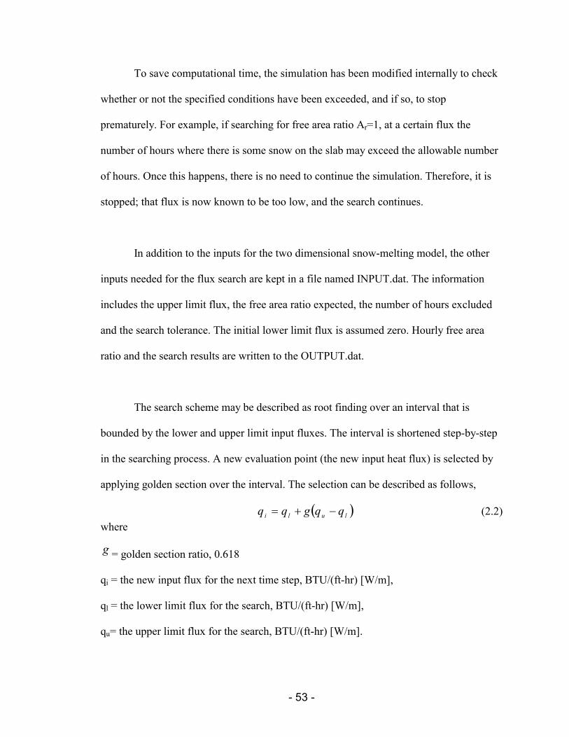
To save computational time, the simulation has been modified internally to check
whether or not the specified conditions have been exceeded, and if so, to stop
prematurely. For example, if searching for free area ratio Ar=1, at a certain flux the
number of hours where there is some snow on the slab may exceed the allowable number
of hours. Once this happens, there is no need to continue the simulation. Therefore, it is
stopped; that flux is now known to be too low, and the search continues.
In addition to the inputs for the two dimensional snow-melting model, the other
inputs needed for the flux search are kept in a file named INPUT.dat. The information
includes the upper limit flux, the free area ratio expected, the number of hours excluded
and the search tolerance. The initial lower limit flux is assumed zero. Hourly free area
ratio and the search results are written to the OUTPUT.dat.
The search scheme may be described as root finding over an interval that is
bounded by the lower and upper limit input fluxes. The interval is shortened step-by-step
in the searching process. A new evaluation point (the new input heat flux) is selected by
applying golden section over the interval. The selection can be described as follows,
q (2.2) � luli qqgq ��� �where
g = golden section ratio, 0.618
qi = the new input flux for the next time step, BTU/(ft-hr) [W/m],
ql = the lower limit flux for the search, BTU/(ft-hr) [W/m],
qu= the upper limit flux for the search, BTU/(ft-hr) [W/m].
- 53 -

At any step in the search, a lower limit flux and upper limit flux will have already
been determined. If the simulation using the input flux at the evaluation point allows the
required conditions to be met, this input flux becomes the new upper limit. Otherwise, it
becomes the new lower limit.
For the cases that the expected free area ratio is nonzero, if current flux input is
lower than required, the program looks for the last hour index where the free area ratio is
less than the requirement. For the cases that the expected free area ratio equals to zero,
the program searches the last hour index that the snow height increases. The value of this
hour number is set as the length for the next simulation.
- 54 -
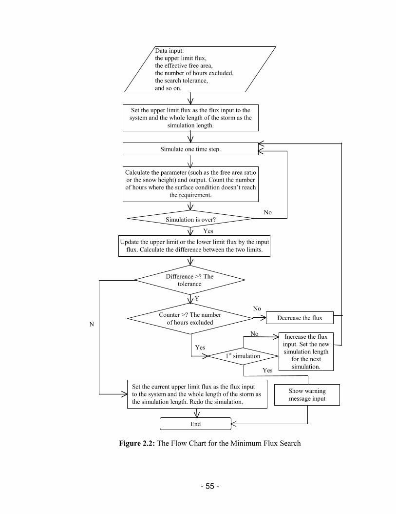
simulation.
s Show warning message input
Yes
No
1st simulation Yes
NoY
No
Set the current upper limit flux as the flux input to the system and the whole length of the storm athe simulation length. Redo the simulation.
End
Difference >? Thetolerance
Update the upper limit or the lower limit flux by the input flux. Calculate the difference between the two limits.
Increase the flux input. Set the new simulation length
for the next
Simulation is over?
Decrease the flux Counter >? The number of hours excluded
Calculate the parameter (such as the free area ratio or the snow height) and output. Count the number of hours where the surface condition doesn’t reach
the requirement.
Simulate one time step.
Set the upper limit flux as the flux input to the system and the whole length of the storm as the
simulation length.
Data input: the upper limit flux, the effective free area, the number of hours excluded, the search tolerance, and so on.
Yes
N
Figure 2.2: The Flow Chart for the Minimum Flux Search
- 55 -
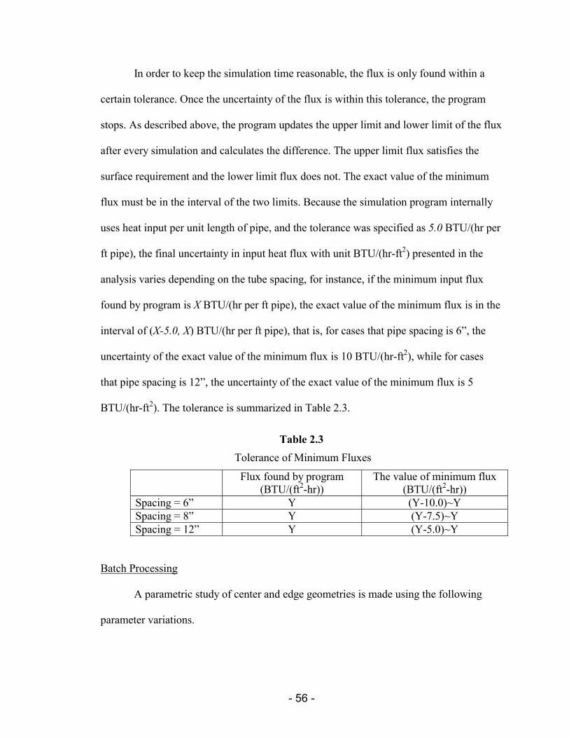
In order to keep the simulation time reasonable, the flux is only found within a
certain tolerance. Once the uncertainty of the flux is within this tolerance, the program
stops. As described above, the program updates the upper limit and lower limit of the flux
after every simulation and calculates the difference. The upper limit flux satisfies the
surface requirement and the lower limit flux does not. The exact value of the minimum
flux must be in the interval of the two limits. Because the simulation program internally
uses heat input per unit length of pipe, and the tolerance was specified as 5.0 BTU/(hr per
ft pipe), the final uncertainty in input heat flux with unit BTU/(hr-ft2) presented in the
analysis varies depending on the tube spacing, for instance, if the minimum input flux
found by program is X BTU/(hr per ft pipe), the exact value of the minimum flux is in the
interval of (X-5.0, X) BTU/(hr per ft pipe), that is, for cases that pipe spacing is 6”, the
uncertainty of the exact value of the minimum flux is 10 BTU/(hr-ft2), while for cases
that pipe spacing is 12”, the uncertainty of the exact value of the minimum flux is 5
BTU/(hr-ft2). The tolerance is summarized in Table 2.3.
Table 2.3 Tolerance of Minimum Fluxes
Flux found by program (BTU/(ft2-hr))
The value of minimum flux (BTU/(ft2-hr))
Spacing = 6” Y (Y-10.0)~Y Spacing = 8” Y (Y-7.5)~Y Spacing = 12” Y (Y-5.0)~Y
Batch Processing
A parametric study of center and edge geometries is made using the following
parameter variations.
- 56 -

�� 10 locations (Spokane, Reno, SLC, Springs in Colorado, Chicago, OKC,
Minneapolis, Buffalo, Boston, Philadelphia)
�� 2 storms at each location (99%-tile Ar=1, 99%-tile Ar=0)
�� Insulated and un-insulated slabs
�� 3 pipe spacing
�� 2 pipe depth
�� 2 soil conductivities
It represents 360 combinations of location, storm and configuration. A batch
command file is used to deal with the cases automatically. Through batch processing,
groups of simulations could be run on different computers at different time. Batch
command files are generated using a program created in Visual Basic.
2.2.3. Methodology of Edge Zone Parametric Study
Because the edge zone parametric study doesn’t require searching for the
minimum flux, a similar but simpler approach than that used for the center zone
parametric study is utilized. The batch processing is similar.
2.3. Results and Discussion
2.3.1. Center Zone Parametric Study
2.3.1.1.Case Ar=1
Table 2.4 and Table 2.5 show the results for the center zone parametric studies
with expected free area ratio 1. The minimum fluxes for each combination of the
- 57 -
parameters are tabulated in Table 2.4. The fluxes maintain a free area ratio of 1 for the
entire storm, except the number of hours where the steady-state design load exceeded the
99% non-exceedance level. The 99% non-exceedance loads can be found from the
ASHRAE handbook.
By normalizing the minimum fluxes against the 99% non-exceedance loads, it
shows more clearly in Table 2.5 the relationship between the steady-state design loads
without back losses and the actual transient load with back losses. Looking at Table 2.5,
the following observation may be made:
��Several searches are stopped due to the flux requirement exceeded the upper limit
(900 Btu/h-ft2). The very high flux requirements indicate it’s impractical to
achieve the design goal that maintains the surface free of snow when the system is
operated without idling. The high flux requirements generally occur when storms
start with relatively high calculated steady-state loads. Without idling, very high
fluxes are required to raise the slab temperature sufficiently at the start of the
storm.
��The results are most sensitive to the storm itself. This will be discussed in more
detail below. Briefly, it has been noted that storms that start off with relatively
low loads, perhaps even ceasing to snow for a few hours, then increasing in
intensity, will have much lower ratios than storms that start off with high load.
��After the storm itself, the results are most sensitive to the spacing. The farther
apart the tubes, the more difficult it is to maintain a completely snow-free surface.
Also, as the tubes are placed deeper, the effect of spacing is less important.
- 58 -
��The results are somewhat less sensitive to the depth of the tubing. Generally, the
depth is more important for the storms that are intense early on. With storms that
are less intense in the early hours, the depth make relatively little difference.
Furthermore, there are a significant number of scenarios where increasing the
depth decreases the flux requirement.
��The results are almost completely insensitive to the soil conductivity and whether
or not insulation has been installed.
Also, unless further research proves otherwise, we would not assume that the
storms are typical of the location. Currently, we would not draw the conclusion by
locations. A better way to draw conclusions is to categorize the results by storms.
Sensitivity to Storm
As stated above, the most important factor for the load is the storm itself. To
illustrate the sensitivity to the storm, we might first consider storms where the ratios of
the minimum required heat flux to the 99% steady-state load are fairly high, in Spokane
and Oklahoma City. Weather data for these storms are plotted in Figures 2.3 and 2.4. The
top plot of each figure shows the weather conditions; the bottom plot shows the steady-
state design loads calculated for each hour.
- 59 -
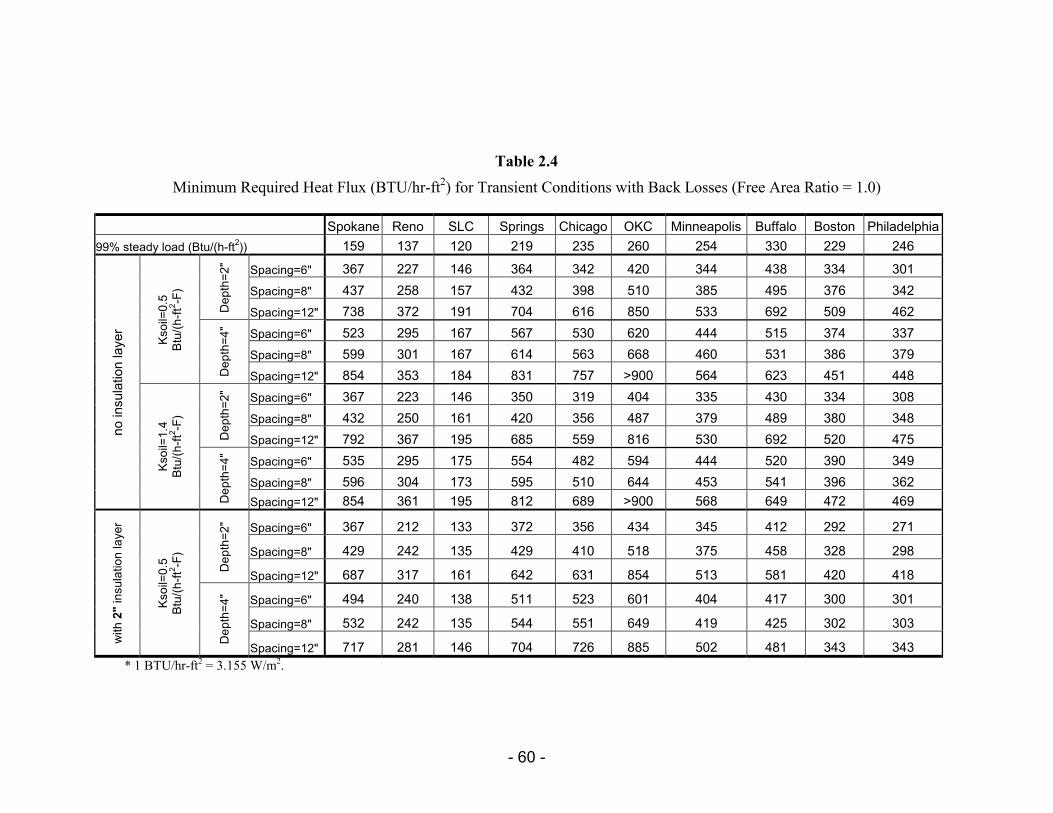
Table 2.4 Minimum Required Heat Flux (BTU/hr-ft2) for Transient Conditions with Back Losses (Free Area Ratio = 1.0)
* 1 B /hr-ft2 = 3.155 W/m . TU 2
Spokane Reno SLC Springs Chicago OKC Minneapolis Buffalo Boston Philadelphia99% steady load (Btu/(h-ft2)) 159 137 120 219 235 260 254 330 229 246
Spacing=6" 367 227 146 364 342 420 344 438 334 301Spacing=8" 437 258 157 432 398 510 385 495 376 342
Dep
th=2
"
Spacing=12" 738 372 191 704 616 850 533 692 509 462Spacing=6" 523 295 167 567 530 620 444 515 374 337Spacing=8" 599 301 167 614 563 668 460 531 386 379
Ksoi
l=0.
5
Btu/
(h-ft
2 -F)
Dep
th=4
"
Spacing=12" 854 353 184 831 757 >900 564 623 451 448Spacing=6" 367 223 146 350 319 404 335 430 334 308Spacing=8" 432 250 161 420 356 487 379 489 380 348
Dep
th=2
"
Spacing=12" 792 367 195 685 559 816 530 692 520 475Spacing=6" 535 295 175 554 482 594 444 520 390 349Spacing=8" 596 304 173 595 510 644 453 541 396 362
no in
sula
tion
laye
r
Ksoi
l=1.
4
Btu/
(h-ft
2 -F)
Dep
th=4
"
Spacing=12" 854 361 195 812 689 >900 568 649 472 469
Spacing=6" 367 212 133 372 356 434 345 412 292 271
Spacing=8" 429 242 135 429 410 518 375 458 328 298
Dep
th=2
"
Spacing=12" 687 317 161 642 631 854 513 581 420 418
Spacing=6" 494 240 138 511 523 601 404 417 300 301
Spacing=8" 532 242 135 544 551 649 419 425 302 303
with
2"
insu
latio
n la
yer
Ksoi
l=0.
5
Btu/
(h-ft
2 -F)
Dep
th=4
"
Spacing=12" 717 281 146 704 726 885 502 481 343 343
- 60 -
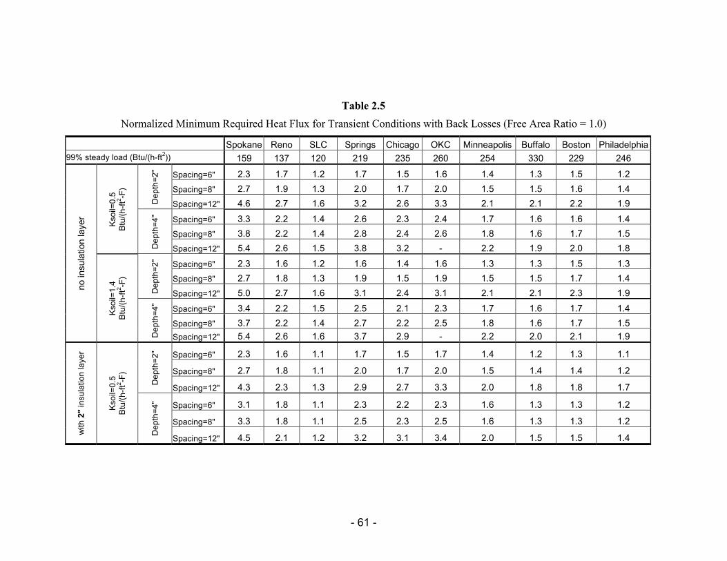
Table 2.5 Normalized Minimum Required Heat Flux for Transient Conditions with Back Losses (Free Area Ratio = 1.0)
Spokane Reno SLC Springs Chicago OKC Minneapolis Buffalo Boston Philadelphia99% steady load (Btu/(h-ft2)) 159 137 120 219 235 260 254 330 229 246
Spacing=6" 2.3 1.7 1.2 1.7 1.5 1.6 1.4 1.3 1.5 1.2Spacing=8" 2.7 1.9 1.3 2.0 1.7 2.0 1.5 1.5 1.6 1.4
Dep
th=2
"
Spacing=12" 4.6 2.7 1.6 3.2 2.6 3.3 2.1 2.1 2.2 1.9
Spacing=6" 3.3 2.2 1.4 2.6 2.3 2.4 1.7 1.6 1.6 1.4Spacing=8" 3.8 2.2 1.4 2.8 2.4 2.6 1.8 1.6 1.7 1.5
Ksoi
l=0.
5
Btu/
(h-ft
2 -F)
Dep
th=4
"
Spacing=12" 5.4 2.6 1.5 3.8 3.2 - 2.2 1.9 2.0 1.8
Spacing=6" 2.3 1.6 1.2 1.6 1.4 1.6 1.3 1.3 1.5 1.3Spacing=8" 2.7 1.8 1.3 1.9 1.5 1.9 1.5 1.5 1.7 1.4
Dep
th=2
"
Spacing=12" 5.0 2.7 1.6 3.1 2.4 3.1 2.1 2.1 2.3 1.9Spacing=6" 3.4 2.2 1.5 2.5 2.1 2.3 1.7 1.6 1.7 1.4Spacing=8" 3.7 2.2 1.4 2.7 2.2 2.5 1.8 1.6 1.7 1.5
no in
sula
tion
laye
r
Ksoi
l=1.
4
B-ft
2 -tu
/(hF)
Dep
th=4
"
Spacing=12" 5.4 2.6 1.6 3.7 2.9 - 2.2 2.0 2.1 1.9
Spacing=6" 2.3 1.6 1.1 1.7 1.5 1.7 1.4 1.2 1.3 1.1
Spacing=8" 2.7 1.8 1.1 2.0 1.7 2.0 1.5 1.4 1.4 1.2
Dep
th=2
"
Spacing=12" 4.3 2.3 1.3 2.9 2.7 3.3 2.0 1.8 1.8 1.7
Spacing=6" 3.1 1.8 1.1 2.3 2.2 2.3 1.6 1.3 1.3 1.2
Spacing=8" 3.3 1.8 1.1 2.5 2.3 2.5 1.6 1.3 1.3 1.2
with
2"
insu
latio
n la
yer
Ksoi
l=0.
5
Btu/
(h-ft
2 -F)
Dep
th=4
"
Spacing=12" 4.5 2.1 1.2 3.2 3.1 3.4 2.0 1.5 1.5 1.4
- 61 -
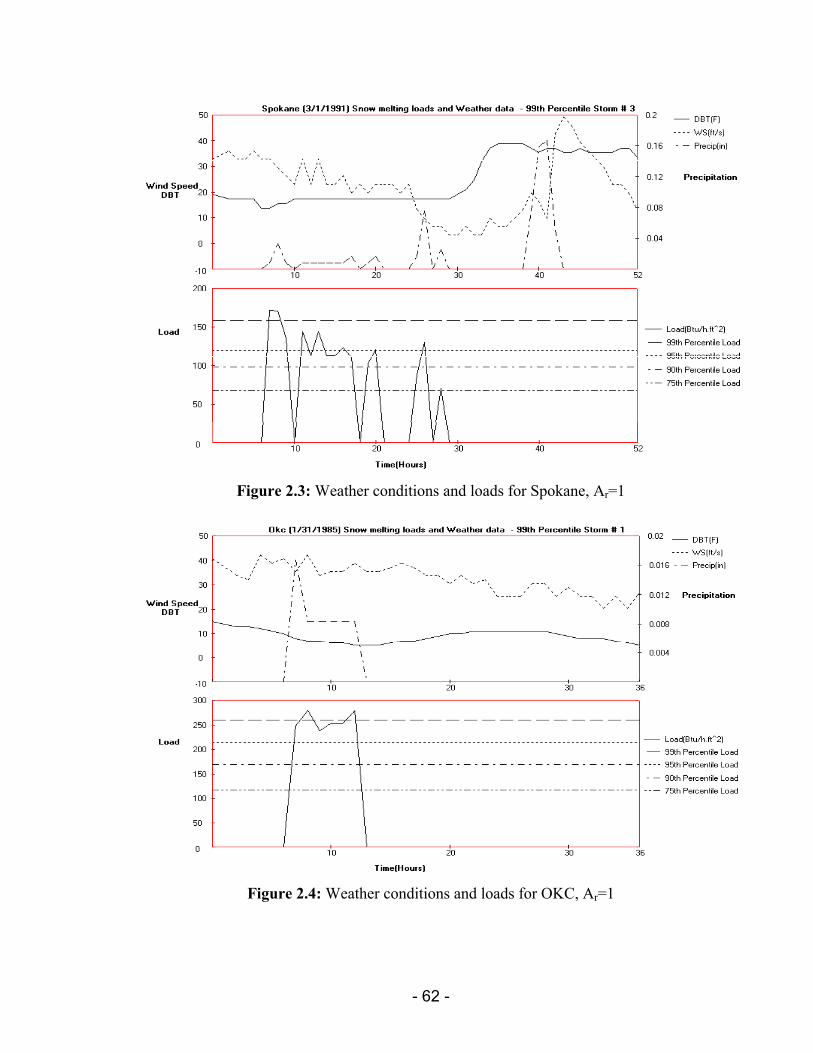
Figure 2.3: Weather conditions and loads for Spokane, Ar=1
Figure 2.4: Weather conditions and loads for OKC, Ar=1
- 62 -
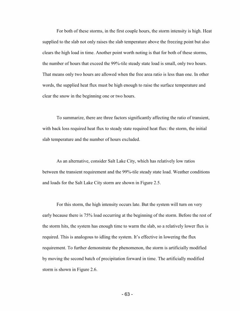
For both of these storms, in the first couple hours, the storm intensity is high. Heat
supplied to the slab not only raises the slab temperature above the freezing point but also
clears the high load in time. Another point worth noting is that for both of these storms,
the number of hours that exceed the 99%-tile steady state load is small, only two hours.
That means only two hours are allowed when the free area ratio is less than one. In other
words, the supplied heat flux must be high enough to raise the surface temperature and
clear the snow in the beginning one or two hours.
To summarize, there are three factors significantly affecting the ratio of transient,
with back loss required heat flux to steady state required heat flux: the storm, the initial
slab temperature and the number of hours excluded.
As an alternative, consider Salt Lake City, which has relatively low ratios
between the transient requirement and the 99%-tile steady state load. Weather conditions
and loads for the Salt Lake City storm are shown in Figure 2.5.
For this storm, the high intensity occurs late. But the system will turn on very
early because there is 75% load occurring at the beginning of the storm. Before the rest of
the storm hits, the system has enough time to warm the slab, so a relatively lower flux is
required. This is analogous to idling the system. It’s effective in lowering the flux
requirement. To further demonstrate the phenomenon, the storm is artificially modified
by moving the second batch of precipitation forward in time. The artificially modified
storm is shown in Figure 2.6.
- 63 -
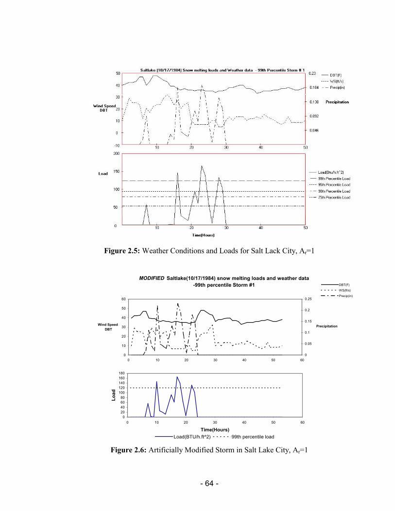
Figure 2.5: Weather Conditions and Loads for Salt Lack City, Ar=1
Figure 2.6: Artificially Modified Storm in Salt Lake City, Ar=1
MODIFIED Saltlake(10/17/1984) snow melting loads and weather data-99th percentile Storm #1
0
10
20
30
40
50
60
0 10 20 30 40 50 60
Wind Speed DBT
0
0.05
0.1
0.15
0.2
0.25
Precipitation
DBT(F)
WS(ft/s)
Precip(in)
020406080
100120140160180
0 10 20 30 40 50 60
Time(Hours)
Load
Load(BTU/h.ft^2) 99th percentile load
- 64 -

For the case with no insulation, soil conductivity of 0.5 Btu/(h-ft2-F), spacing 12”,
the minimum heat flux required with the original storm is 191 Btu/(h-ft2). While with the
artificial modified storm, it increases to 229 Btu/(h-ft2). This represents an increase in the
ratio from 1.6 to 1.9.
More examples are available to demonstrate the importance of the actual snowfall
pattern on the ratio required heat flux for transient conditions. If a free area ratio of one is
absolutely required, idling at some level will probably be necessary. On the other hand, if
some time lag in clearing off the snow is allowable, then the steady state heat fluxes or
moderately increased heat fluxes might be acceptable.
Effect of Depth on the Minimum Flux Requirement
It might be expected that the deeper tubing would increase the heat flux
requirement due to the slower response of the surface flux to the source. However, there
are a large number of cases where increasing the depth either decreases the heat flux
requirement or has a negligible influence. The cases generally occur in the storms for
which the high intensity hours come late and the normalized flux requirement ratios are
relatively low. For this type of storm, the latter hours of the storm are more important to
maintain the expected requirement. It makes the additional time delay caused by the
deeper tubing not significant. Conversely, for storms with relatively high ratios, the
deeper the tubing, the more likely it is that the flux requirement increases. For this type of
storms, the high intensity hours occur early. The response speed of the slab in the first
- 65 -
several hours has the most significant effect on the surface conditions that may be
achieved.
Within any given storm, the wider the spacing, the more likely it is that increasing
the depth of the tubing will decrease the minimum heat flux requirement. The more
uniform heat flux yielded by the deeper tubing allows more uniform melting.
To demonstrate the point above, the concept of the controlling hour is introduced.
It’s very obvious that for any given storm, in the flux searching process, there is one or
two hours that tend to control the required heat flux. For example, decreasing the heat
flux slightly will cause the free area ratio to drop below one for that hour. For the Buffalo
storm, we have studied the surface heat flux and surface conditions for a heat flux of
622.7 BTU/hr-ft2, 12” spacing, and 2” and 4” depths, at the controlling hour, in Figures
2.7 and 2.8. In these plots, the distance “0.0” represents the location above the tube; and
the distance “0.5” would be midway between the tubes. For this hour, the more uniform
heat flux of the deeper pipe allows 622.7 BTU/hr-ft2 to be sufficient for the 4” deep
tubing, but not for 2” deep tubing.
- 66 -
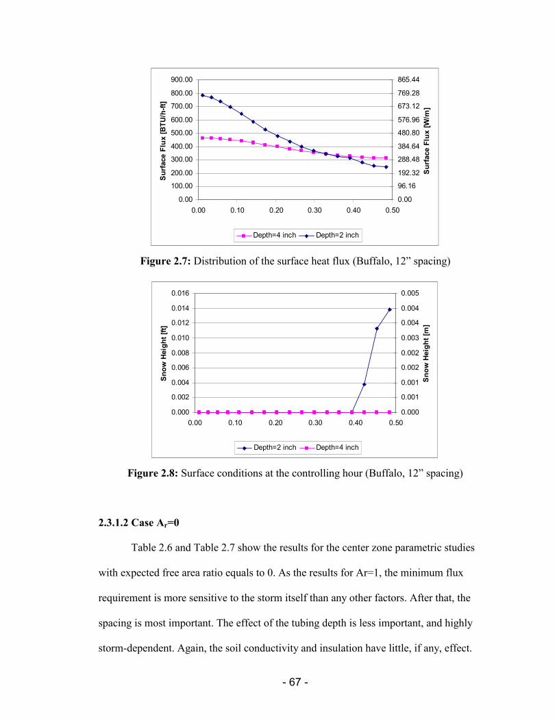
0.00
100.00
200.00
300.00
400.00
500.00
600.00
700.00
800.00
900.00
0.00 0.10 0.20 0.30 0.40 0.50
Surfa
ce F
lux
[BTU
/h-ft
]
0.00
96.16
192.32
288.48
384.64
480.80
576.96
673.12
769.28
865.44
Surfa
ce F
lux
[W/m
]
Depth=4 inch Depth=2 inch
Figure 2.7: Distribution of the surface heat flux (Buffalo, 12” spacing)
0.000
0.002
0.004
0.006
0.008
0.010
0.012
0.014
0.016
0.00 0.10 0.20 0.30 0.40 0.50
Snow
Hei
ght [
ft]
0.000
0.001
0.001
0.002
0.002
0.003
0.004
0.004
0.005
Snow
Hei
ght [
m]
Depth=2 inch Depth=4 inch
Figure 2.8: Surface conditions at the controlling hour (Buffalo, 12” spacing)
2.3.1.2 Case Ar=0
Table 2.6 and Table 2.7 show the results for the center zone parametric studies
with expected free area ratio equals to 0. As the results for Ar=1, the minimum flux
requirement is more sensitive to the storm itself than any other factors. After that, the
spacing is most important. The effect of the tubing depth is less important, and highly
storm-dependent. Again, the soil conductivity and insulation have little, if any, effect.
- 67 -
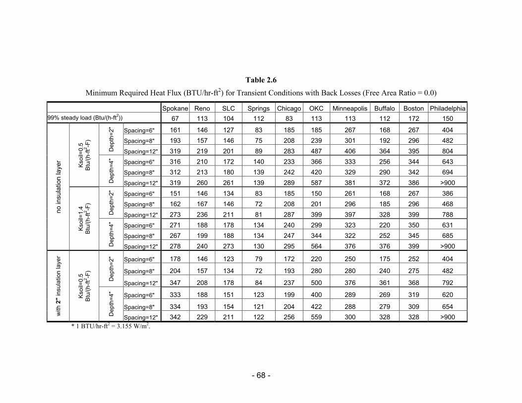
Table 2.6 Minimum Required Heat Flux (BTU/hr-ft2) for Transient Conditions with Back Losses (Free Area Ratio = 0.0)
Spokane Reno SLC Springs Chicago OKC Minneapolis Buffalo Boston Philadelphia99% steady load (Btu/(h-ft2)) 67 113 104 112 83 113 113 112 172 150
Spacing=6" 161 146 127 83 185 185 267 168 267 404Spacing=8" 193 157 146 75 208 239 301 192 296 482
Dep
th=2
"
Spacing=12" 319 219 201 89 283 487 406 364 395 804Spacing=6" 316 210 172 140 233 366 333 256 344 643Spacing=8" 312 213 180 139 242 420 329 290 342 694
Ksoi
l=0.
5
Btu/
(h-ft
2 -F)
Dep
th=4
"
Spacing=12" 319 260 261 139 289 587 381 372 386 >900Spacing=6" 151 146 134 83 185 150 261 168 267 386Spacing=8" 162 167 146 72 208 201 296 185 296 468
Dep
th=2
"
Spacing=12" 273 236 211 81 287 399 397 328 399 788Spacing=6" 271 188 178 134 240 299 323 220 350 631Spacing=8" 267 199 188 134 247 344 322 252 345 685
no in
sula
tion
laye
r
Ksoi
l=1.
4
B-ft
2 -tu
/(hF)
Dep
th=4
"
Spacing=12" 278 240 273 130 295 564 376 376 399 >900
Spacing=6" 178 146 123 79 172 220 250 175 252 404
Spacing=8" 204 157 134 72 193 280 280 240 275 482
Dep
th=2
"
Spacing=12" 347 208 178 84 237 500 376 361 368 792
Spacing=6" 333 188 151 123 199 400 289 269 319 620
Spacing=8" 334 193 154 121 204 422 288 279 309 654
with
2"
insu
latio
n la
yer
Ksoi
l=0.
5
Btu/
(h-ft
2 -F)
Dep
th=4
"
Spacing=12" 342 229 211 122 256 559 300 328 328 >900* 1 BTU/hr-ft2 = 3.155 W/m2.
- 68 -
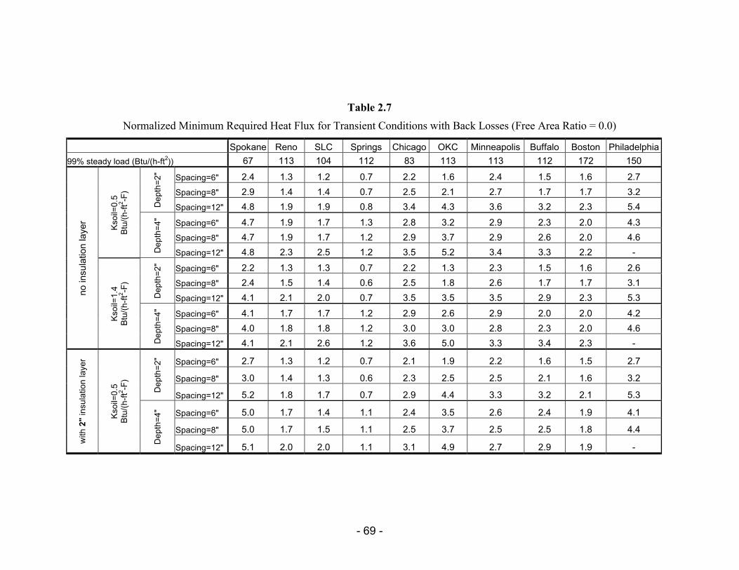
Table 2.7 Normalized Minimum Required Heat Flux for Transient Conditions with Back Losses (Free Area Ratio = 0.0)
Spokane Reno SLC Springs Chicago OKC Minneapolis Buffalo Boston Philadelphia99% steady load (Btu/(h-ft2)) 67 113 104 112 83 113 113 112 172 150
Spacing=6" 2.4 1.3 1.2 0.7 2.2 1.6 2.4 1.5 1.6 2.7Spacing=8" 2.9 1.4 1.4 0.7 2.5 2.1 2.7 1.7 1.7 3.2
Dep
th=2
"
Spacing=12" 4.8 1.9 1.9 0.8 3.4 4.3 3.6 3.2 2.3 5.4
Spacing=6" 4.7 1.9 1.7 1.3 2.8 3.2 2.9 2.3 2.0 4.3Spacing=8" 4.7 1.9 1.7 1.2 2.9 3.7 2.9 2.6 2.0 4.6
Ksoi
l=0.
5
Btu/
(h-ft
2 -F)
Dep
th=4
"
Spacing=12" 4.8 2.3 2.5 1.2 3.5 5.2 3.4 3.3 2.2 -
Spacing=6" 2.2 1.3 1.3 0.7 2.2 1.3 2.3 1.5 1.6 2.6Spacing=8" 2.4 1.5 1.4 0.6 2.5 1.8 2.6 1.7 1.7 3.1
Dep
th=2
"
Spacing=12" 4.1 2.1 2.0 0.7 3.5 3.5 3.5 2.9 2.3 5.3Spacing=6" 4.1 1.7 1.7 1.2 2.9 2.6 2.9 2.0 2.0 4.2Spacing=8" 4.0 1.8 1.8 1.2 3.0 3.0 2.8 2.3 2.0 4.6
no in
sula
tion
laye
r
Ksoi
l=1.
4
B-ft
2 -tu
/(hF)
Dep
th=4
"
Spacing=12" 4.1 2.1 2.6 1.2 3.6 5.0 3.3 3.4 2.3 -
Spacing=6" 2.7 1.3 1.2 0.7 2.1 1.9 2.2 1.6 1.5 2.7
Spacing=8" 3.0 1.4 1.3 0.6 2.3 2.5 2.5 2.1 1.6 3.2
Dep
th=2
"
Spacing=12" 5.2 1.8 1.7 0.7 2.9 4.4 3.3 3.2 2.1 5.3
Spacing=6" 5.0 1.7 1.4 1.1 2.4 3.5 2.6 2.4 1.9 4.1
Spacing=8" 5.0 1.7 1.5 1.1 2.5 3.7 2.5 2.5 1.8 4.4
with
2"
insu
latio
n la
yer
Ksoi
l=0.
5
Btu/
(h-ft
2 -F)
Dep
th=4
"
Spacing=12" 5.1 2.0 2.0 1.1 3.1 4.9 2.7 2.9 1.9 -
- 69 -
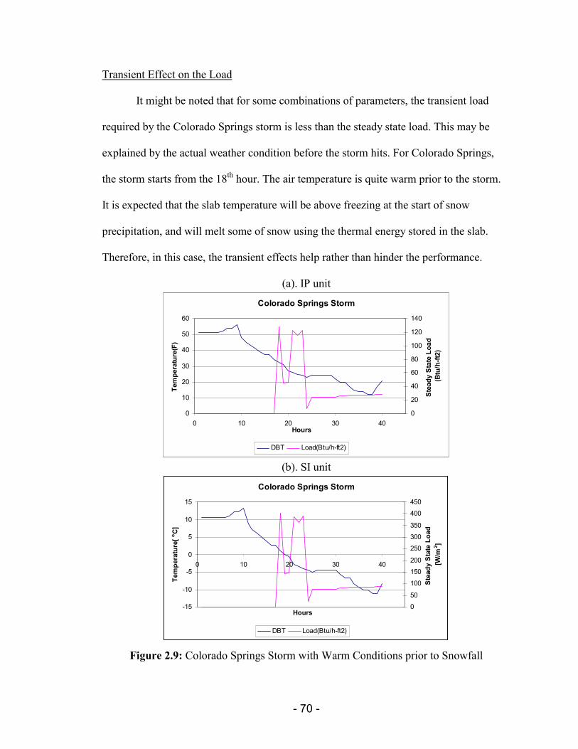
Transient Effect on the Load
It might be noted that for some combinations of parameters, the transient load
required by the Colorado Springs storm is less than the steady state load. This may be
explained by the actual weather condition before the storm hits. For Colorado Springs,
the storm starts from the 18th hour. The air temperature is quite warm prior to the storm.
It is expected that the slab temperature will be above freezing at the start of snow
precipitation, and will melt some of snow using the thermal energy stored in the slab.
Therefore, in this case, the transient effects help rather than hinder the performance.
(a). IP unit
Colorado Springs Storm
0
10
20
30
40
50
60
0 10 20 30 40Hours
Tem
pera
ture
(F)
0
20
40
60
80
100
120
140
Stea
dy S
tate
Loa
d (B
tu/h
-ft2)
DBT Load(Btu/h-ft2)
(b). SI unit
Colorado Springs Storm
-15
-10
-5
0
5
10
15
0 10 20 30 40
Hours
Tem
pera
ture
[o C]
050
100
150200
250300350
400450
Stea
dy S
tate
Loa
d [W
/m2 ]
DBT Load(Btu/h-ft2)
Figure 2.9: Colorado Springs Storm with Warm Conditions prior to Snowfall
- 70 -

2.3.1.3 Back Losses
Designers are interested not only in the minimum flux requirement of the system
but also in the actual back losses. Table 2.8 and Table 2.9 show the results of maximum
percentage back loss for free area ratio of 1 and 0 respectively. Because the back loss
varies every hour, what’s tabulated is the maximum percentage back loss.
The following trends may be observed:
��Insulation is quite effective in reducing the back loss.
��Soil conductivity has significant impact on the back losses.
��The depth is relatively important – the deeper tubing has, as expected, higher back
losses. Naturally, this is more significant for uninsulated slabs and higher
conductivity soil.
��Pipe spacing has less impact on the back losses.
- 71 -
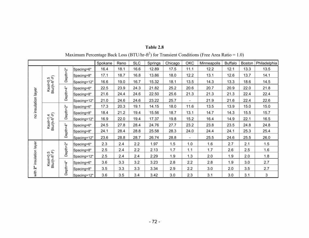
Table 2.8 Maximum Percentage Back Loss (BTU/hr-ft ) for Transient Conditions (Free Area Ratio = 1.0)
Spokane Reno SLC Springs Chicago OKC MinneapolisSpacing=6" 12.89 17.5 11.1
2
Buffalo Boston Philadelphia16.4 18.1 16.6 12.2 13.3 13.5
Spacing=8" 17.1 18.7 16.8 13.86 18.0 12.2 13.1 12.6 13.7 14.1
Dep
th=2
"
Spacing=12" 16.6 19.0 16.7 15.32 18.1 13.5 14.3 13.3 18.6 14.5Spacing=6" 22.5 23.9 24.3 21.82 25.2 20.6 20.7 20.9 22.0 21.8Spacing=8" 21.6 24.4 24.6 22.50 25.6 21.3 21.3 21.3 22.4 22.4
Ksoi
l=0.
5
Btu/
(h-ft
2 -F)
Dep
th=4
"
Spacing=12" 21.0 24.6 24.6 23.22 25.7 - 21.9 21.6 22.4 22.6Spacing=6" 17.3 20.3 19.1 14.15 18.0 11.6 13.5 13.9 15.0 15.0Spacing=8" 18.4 21.2 19.4 15.56 18.7 13.1 14.7 14.3 15.5 15.7
Dep
th=2
"
Spacing=12" 16.9 22.0 19.4 17.37 19.8 15.2 16.4 14.9 22.1 16.5Spacing=6" 24.5 27.8 28.4 24.76 27.7 23.2 23.8 23.5 24.8 24.8Spacing=8" 24.1 28.4 28.8 25.58 28.3 24.0 24.4 24.1 25.3 25.4
no in
sula
tion
laye
r
Ksoi
l=1.
4
B-ft
2 -tu
/(hF)
Dep
th=4
"
Spacing=12" 23.6 28.8 28.7 26.74 28.8 - 25.5 24.6 25.5 26.0Spacing=6" 2.3 2.4 2.2 1.97 1.5 1.0 1.6 2.7 2.1 1.5Spacing=8" 2.5 2.4 2.2 2.13 1.7 1.1 1.7 2.6 2.5 1.6
Dep
th=2
"
Spacing=12" 2.5 2.4 2.4 2.29 1.9 1.3 2.0 1.9 2.0 1.8Spacing=6" 3.6 3.3 3.2 3.23 2.8 2.2 2.8 1.9 3.0 2.7Spacing=8" 3.5 3.3 3.3 3.34 2.9 2.2 3.0 2.0 3.5 2.7
with
2"
insu
latio
n la
yer
Ksoi
l=0.
5
Btu/
(h-ft
2 -F)
Dep
th=4
"
Spacing=12" 3.6 3.5 3.4 3.42 3.0 2.3 3.1 3.0 3.1 3
12.1
- 72 -
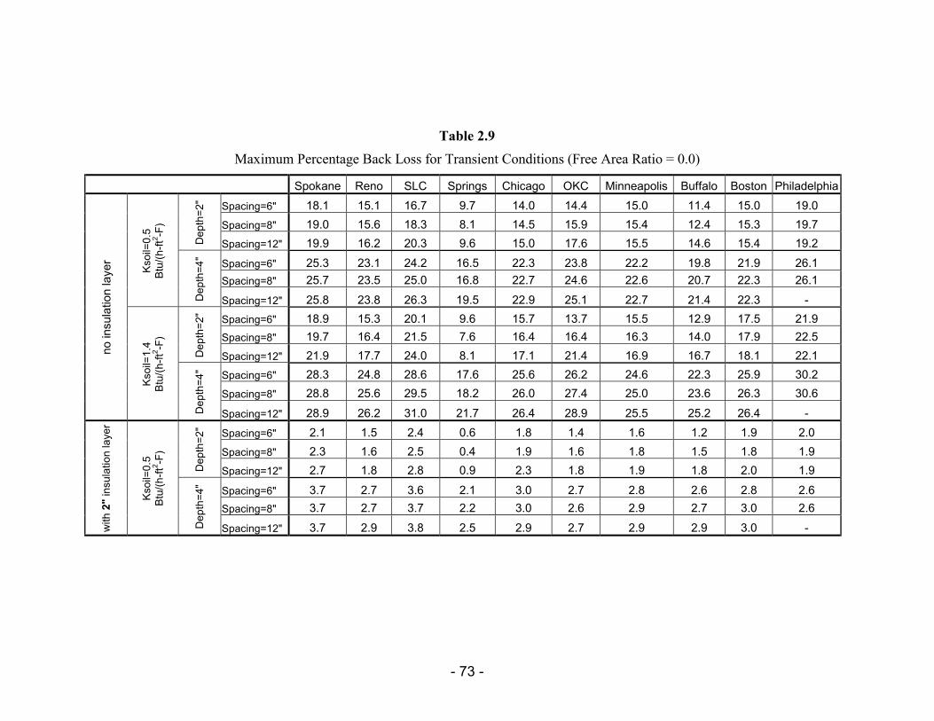
Table 2.9 Maximum Percentage Back Loss for Transient Conditions (Free Area Ratio = 0.0)
Spokane Reno SLC Springs Chicago OKC Minneapolis Buffalo Boston PhiladelphiaSpacing=6" 18.1 15.1 16.7 9.7 14.0 14.4 15.0 11.4 15.0 19.0Spacing=8" 19.0 15.6 18.3 8.1 14.5 15.9 15.4 12.4 15.3 19.7
Dep
th=2
"
Spacing=12" 19.9 16.2 20.3 9.6 15.0 17.6 15.5 14.6 15.4 19.2Spacing=6" 25.3 23.1 24.2 16.5 22.3 23.8 22.2 19.8 21.9 26.1Spacing=8" 25.7 23.5 25.0 16.8 22.7 24.6 22.6 20.7 22.3 26.1
Ksoi
l=0.
5
Btu/
(h-ft
2 -F)
Dep
th=4
"
Spacing=12" 25.8 23.8 26.3 19.5 22.9 25.1 22.7 21.4 22.3 -Spacing=6" 18.9 15.3 20.1 9.6 15.7 13.7 15.5 12.9 17.5 21.9Spacing=8" 19.7 16.4 21.5 7.6 16.4 16.4 16.3 14.0 17.9 22.5
Dep
th=2
"
Spacing=12" 21.9 17.7 24.0 8.1 17.1 21.4 16.9 16.7 18.1 22.1Spacing=6" 28.3 24.8 28.6 17.6 25.6 26.2 24.6 22.3 25.9 30.2Spacing=8" 28.8 25.6 29.5 18.2 26.0 27.4 25.0 23.6 26.3 30.6
no in
sula
tion
laye
r
Ksoi
l=1.
4
B-ft
2 -tu
/(hF)
Dep
th=4
"
Spacing=12" 28.9 26.2 31.0 21.7 26.4 28.9 25.5 25.2 26.4 -Spacing=6" 2.1 1.5 2.4 0.6 1.8 1.4 1.6 1.2 1.9 2.0Spacing=8" 2.3 1.6 2.5 0.4 1.9 1.6 1.8 1.5 1.8 1.9
Dep
th=2
"
Spacing=12" 2.7 1.8 2.8 0.9 2.3 1.8 1.9 1.8 2.0 1.9
Spacing=6" 3.7 2.7 3.6 2.1 3.0 2.7 2.8 2.6 2.8 2.6Spacing=8" 3.7 2.7 3.7 2.2 3.0 2.6 2.9 2.7 3.0 2.6
with
2"
insu
latio
n la
yer
Ksoi
l=0.
5
Btu/
(h-ft
2 -F)
Dep
th=4
"
Spacing=12" 3.7 2.9 3.8 2.5 2.9 2.7 2.9 2.9 3.0 -
- 73 -
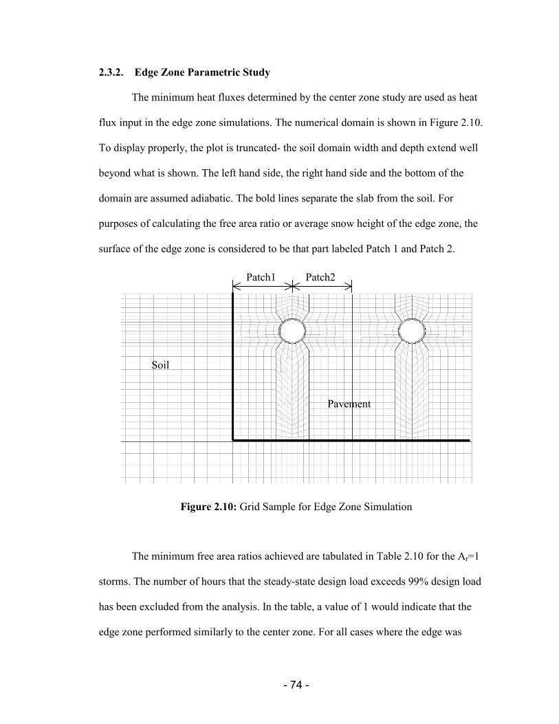
2.3.2. Edge Zone Parametric Study
The minimum heat fluxes determined by the center zone study are used as heat
flux input in the edge zone simulations. The numerical domain is shown in Figure 2.10.
To display properly, the plot is truncated- the soil domain width and depth extend well
beyond what is shown. The left hand side, the right hand side and the bottom of the
domain are assumed adiabatic. The bold lines separate the slab from the soil. For
purposes of calculating the free area ratio or average snow height of the edge zone, the
surface of the edge zone is considered to be that part labeled Patch 1 and Patch 2.
Soil
Pavement
Patch2Patch1
Figure 2.10: Grid Sample for Edge Zone Simulation
The minimum free area ratios achieved are tabulated in Table 2.10 for the Ar=1
storms. The number of hours that the steady-state design load exceeds 99% design load
has been excluded from the analysis. In the table, a value of 1 would indicate that the
edge zone performed similarly to the center zone. For all cases where the edge was
- 74 -

insulated with 2”(50mm) of insulation, the edge zone performed similar to the center
zone as expected. That is, the edge zone was completely snow free by the time the center
zone was completely snow free.
For cases that the edge zone was not insulated, it can be observed that the
performance has been degraded. The heat flux supplied to the pipe is the minimum flux
for the center zone that maintains the free area ratio of 1. For edge zone cases without the
insulation, this heat flux can’t maintain the expected free area ratio. The ratio is still very
close to one, indicating that only at the very edge was the performance degradation
significant.
As expected, higher soil conductivity and deeper tube depth cause more
degradation in performance. Higher tube spacing generally appears to have better
performance. This may be specious, as the analysis area (Patch 1 and Patch 2) increase
with higher tube spacing. Presumably, smaller tube spacing should give better
performance near the edge.
- 75 -
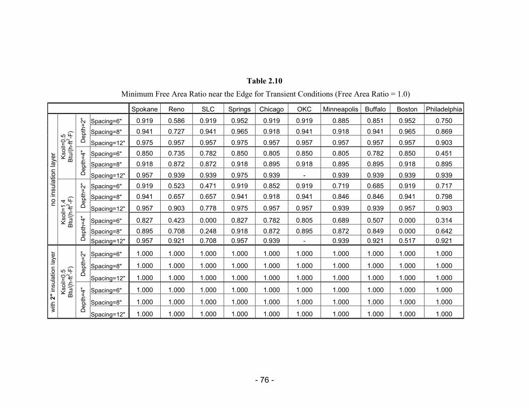
Table 2.10 Minimum Free Area Ratio near the Edge for Transient Conditions (Free Area Ratio = 1.0)
Spokane Reno SLC Springs Chicago OKC Minneapolis Buffalo Boston Philadelphia
Spacing=6" 0.919 0.586 0.919 0.952 0.919 0.919 0.885 0.851 0.952 0.750Spacing=8" 0.941 0.727 0.941 0.965 0.918 0.941 0.918 0.941 0.965 0.869
Dep
th=2
"
Spacing=12" 0.975 0.957 0.957 0.975 0.957 0.957 0.957 0.957 0.957 0.903Spacing=6" 0.850 0.735 0.782 0.850 0.805 0.850 0.805 0.782 0.850 0.451Spacing=8" 0.918 0.872 0.872 0.918 0.895 0.918 0.895 0.895 0.918 0.895
Ksoi
l=0.
5
Btu/
(h-ft
2 -F)
Dep
th=4
"
Spacing=12" 0.957 0.939 0.939 0.975 0.939 - 0.939 0.939 0.939 0.939Spacing=6" 0.919 0.523 0.471 0.919 0.852 0.919 0.719 0.685 0.919 0.717Spacing=8" 0.941 0.657 0.657 0.941 0.918 0.941 0.846 0.846 0.941 0.798
Dep
th=2
"
Spacing=12" 0.957 0.903 0.778 0.975 0.957 0.957 0.939 0.939 0.957 0.903
Spacing=6" 0.827 0.423 0.000 0.827 0.782 0.805 0.689 0.507 0.000 0.314Spacing=8" 0.895 0.708 0.248 0.918 0.872 0.895 0.872 0.849 0.000 0.642
no in
sula
tion
laye
r Ks
oil=
1.4
Bt
u/(h
-ft2 -F
)
Dep
th=4
"
Spacing=12" 0.957 0.921 0.708 0.957 0.939 - 0.939 0.921 0.517 0.921
Spacing=6" 1.000 1.000 1.000 1.000 1.000 1.000 1.000 1.000 1.000 1.000
Spacing=8" 1.000 1.000 1.000 1.000 1.000 1.000 1.000 1.000 1.000 1.000
Dep
th=2
"
Spacing=12" 1.000 1.000 1.000 1.000 1.000 1.000 1.000 1.000 1.000 1.000
Spacing=6" 1.000 1.000 1.000 1.000 1.000 1.000 1.000 1.000 1.000 1.000
Spacing=8" 1.000 1.000 1.000 1.000 1.000 1.000 1.000 1.000 1.000 1.000
with
2"
insu
latio
n la
yer
Ksoi
l=0.
5
Btu/
(h-ft
2 -F)
Dep
th=4
"
Spacing=12" 1.000 1.000 1.000 1.000 1.000 1.000 1.000 1.000 1.000 1.000
- 76 -
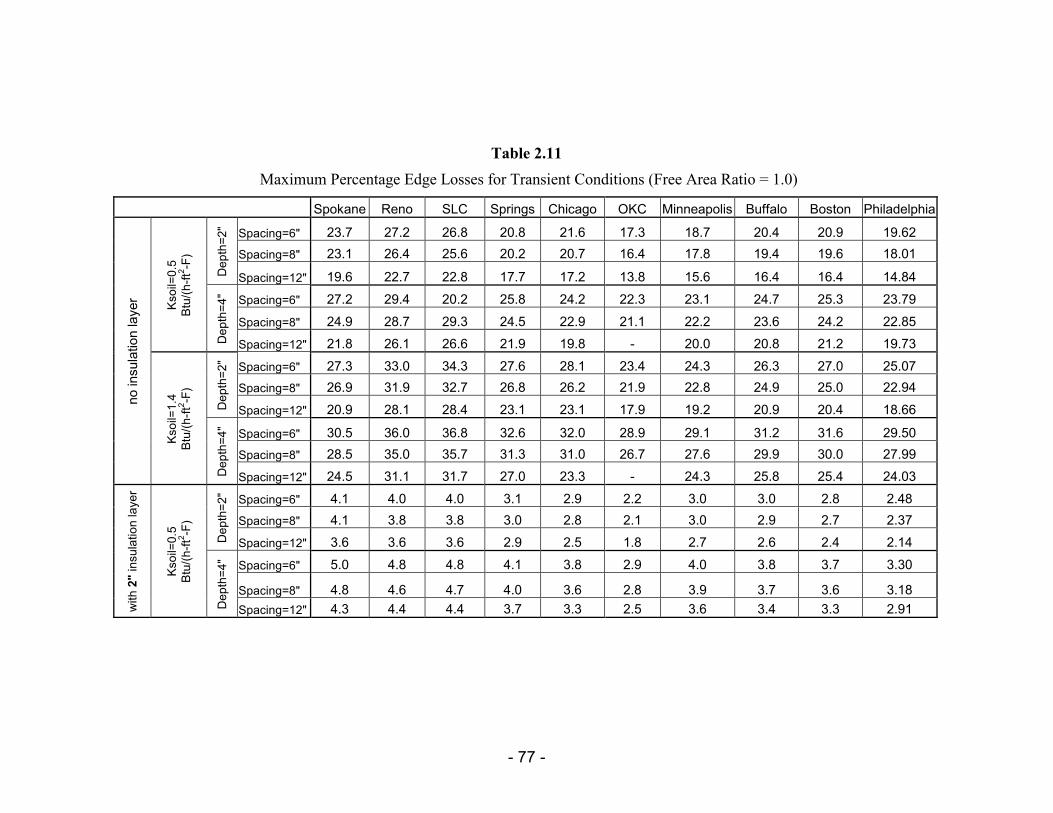
Table 2.11 Maximum Percentage Edge Losses for Transient Conditions (Free Area Ratio = 1.0)
Spokane Reno SLC Springs Chicago OKC Minneapolis Buffalo Boston Philadelphia
Spacing=6" 23.7 27.2 26.8 20.8 21.6 17.3 18.7 20.4 20.9 19.62Spacing=8" 23.1 26.4 25.6 20.2 20.7 16.4 17.8 19.4 19.6 18.01
Dep
th=2
"
Spacing=12" 19.6 22.7 22.8 17.7 17.2 13.8 15.6 16.4 16.4 14.84
Spacing=6" 27.2 29.4 20.2 25.8 24.2 22.3 23.1 24.7 25.3 23.79
Spacing=8" 24.9 28.7 29.3 24.5 22.9 21.1 22.2 23.6 24.2 22.85
Ksoi
l=0.
5
Btu/
(h-ft
2 -F)
Dep
th=4
"
Spacing=12" 21.8 26.1 26.6 21.9 19.8 - 20.0 20.8 21.2 19.73
Spacing=6" 27.3 33.0 34.3 27.6 28.1 23.4 24.3 26.3 27.0 25.07Spacing=8" 26.9 31.9 32.7 26.8 26.2 21.9 22.8 24.9 25.0 22.94
Dep
th=2
"
Spacing=12" 20.9 28.1 28.4 23.1 23.1 17.9 19.2 20.9 20.4 18.66
Spacing=6" 30.5 36.0 36.8 32.6 32.0 28.9 29.1 31.2 31.6 29.50Spacing=8" 28.5 35.0 35.7 31.3 31.0 26.7 27.6 29.9 30.0 27.99
no in
sula
tion
laye
r
Ksoi
l=1.
4
B-ft
2 -tu
/(hF)
Dep
th=4
"
Spacing=12" 24.5 31.1 31.7 27.0 23.3 - 24.3 25.8 25.4 24.03
Spacing=6" 4.1 4.0 4.0 3.1 2.9 2.2 3.0 3.0 2.8 2.48Spacing=8" 4.1 3.8 3.8 3.0 2.8 2.1 3.0 2.9 2.7 2.37
Dep
th=2
"
Spacing=12" 3.6 3.6 3.6 2.9 2.5 1.8 2.7 2.6 2.4 2.14
Spacing=6" 5.0 4.8 4.8 4.1 3.8 2.9 4.0 3.8 3.7 3.30
Spacing=8" 4.8 4.6 4.7 4.0 3.6 2.8 3.9 3.7 3.6 3.18
with
2"
insu
latio
n la
yer
Ksoi
l=0.
5
Btu/
(h-ft
2 -F)
Dep
th=4
"
Spacing=12" 4.3 4.4 4.4 3.7 3.3 2.5 3.6 3.4 3.3 2.91
- 77 -
2.4. Conclusion of Parametric Study
The parametric study of snow-melting systems investigates the effects of transient
conditions, back losses, tube spacing, tube depth, insulation, and soil conductivity on
system performance. Key findings for cases with free area ratio of one include:
�� The 99% steady-state non-exceedance loads are not closely correlated to the
performance of the system under transient conditions with back losses. The heat flux
required to maintain the pavement snow-free for the number of hours with steady-
state loads less than the 99% non-exceedance loads, may be from 1 to 5 times as high
as the 99% non-exceedance load.
�� For some cases, the flux requirement exceeds the level that is feasible to obtain in
practice. It indicates that in many situations, it’s impractical to meet the design goal
of maintaining a free area ratio of one. In these cases, idling is suggested.
�� More than any other factor, the results are most sensitive to the storm itself. Storms
that start off with relatively low loads, perhaps even ceasing to snow for a few hours,
then increasing in intensity, will have much lower ratios of heat flux requirement
than the storms that start off with high loads.
�� After the storm, the results are most sensitive to pipe spacing. The farther apart the
tubes, the more difficult it is to maintain free area ratio of one. As the tubes are
placed deeper, the effect of spacing is less important.
�� The flux requirements are almost insensitive to the soil conductivity and the
insulation level. Insulation is useful for reducing back losses, particularly as the
snow event increases in time.
- 78 -
For a free area ratio of zero, the results are much more difficult to interpret. With
respect to the importance of the storm, the tube spacing, and the tube depth, the results
are similar to those for a free area ratio of one. However, with respect to the ratio
between the heat flux required under the transient conditions to the 99% non-exceedance
load, the results of a free area ratio of zero depend highly on how the concept of a free
area ratio of zero is mapped to transient conditions. In the parametric study, free area
ratio of zero is interpreted as the equivalent dynamic condition that the snow height does
not increase for any more hours beyond the number that exceed the 99% non-exceedance
load. This has resulted in some cases for which there is very little snow on the slab edges,
and a higher flux was required to decrease the snow height near the edges while at the
other area of the surface, the snow height has already stopped increasing. An alternative
(untried) would be to interpret free area ratio of zero as the condition where the slab may
be entirely covered during all hours of storm.
- 79 -
3. Modeling the Bridge Deck by Transfer Function Method
3.1. Introduction
The BFC-FV model described in Chapter 2 uses a finite volume solver to
calculate the temperature distribution of the slab and surroundings. This method requires
a large amount of program storage space and must go through the time consuming
procedure of calculating temperatures, such as nodal temperatures inside the slab, which
are not needed in the analysis of the surface conditions. An alternative is to replace the
finite volume solver with a time series technique that improves both the speed and
storage requirements.
One type of time series solution is the transfer function method, which relates the
current flux via a linear, algebraic equation to flux and temperature histories. For the flux
at one surface of an element, because it only relates to the series of temperature and flux
histories at the both surfaces, and the history of heat sources or sinks inside the element,
there is no need to calculate the other inside nodal temperatures, thus, the transfer
function method becomes much more computationally efficient.
This chapter aims at developing a bridge deck model by heat source transfer
function method (Strand, 1995, 1997). This new model, abbreviated to QTF model, is
expected to be used as a design and simulation tool for modeling the performance of
hydronic and electric-cable heating system. The QTF model can calculate one-
dimensional or two-dimensional heat transfer depending on the transfer function
- 80 -
coefficients supplied to the model. The model is tested by comparing simulation results to
analytical solutions and the results from other simulation programs.
3.2. Modeling by Transfer Function Method
3.2.1. Heat Transfer in Bridge Decks
Conduction through the deck material and convection due to the flow of the heat
transfer fluid are the two heat transfer mechanisms within the bridge deck. The heat
transfer due to the hot fluid is taken as an internal source of the bridge deck.
Without heating, the conduction heat transfer within the bridge deck can be
solved by the conduction transfer functions (CTFs) as a common slab. Strand (1995) has
developed and verified heat source transfer functions (QTFs) that are similar in form to
the standard CTFs for the low temperature radiant heating systems. The QTFs may be
derived from either a Laplace transform or a state space method, and the heat source
transmitted to the slab is treated as a definable, variable input.
The QTF model in this thesis solves the heat transfer within the bridge deck by
heat source transfer functions. A program that generates transfer funcitons, the “QTF
calculator”, developed by Strand (1995), has been used to provide the transfer function
coefficients to the model prior to the simulation. Figure 3.1 shows a typical arrangement
of bridge heating pipe loop. In the one-dimensional heat transfer problem, the heat source
described is planar and evenly distributed along the X direction. In the two-dimensional
- 81 -
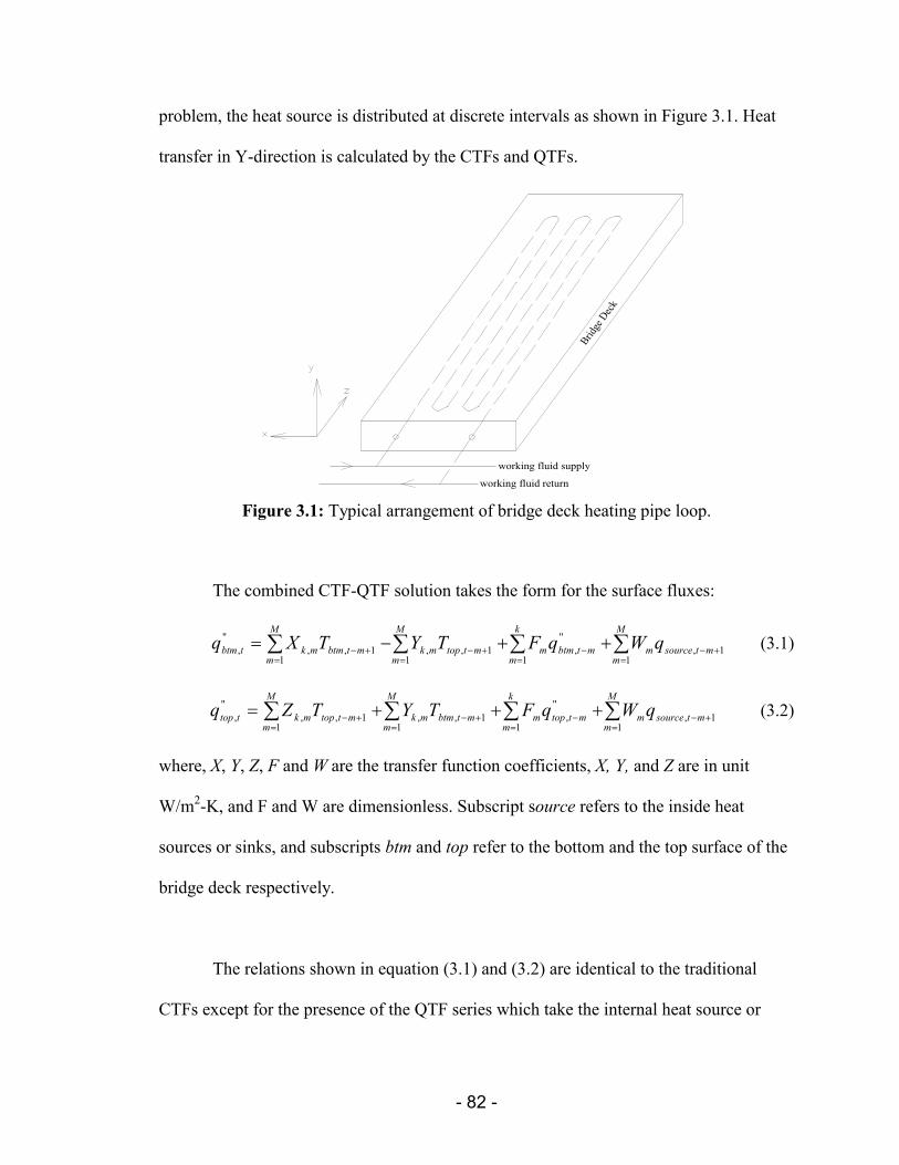
problem, the heat source is distributed at discrete intervals as shown in Figure 3.1. Heat
transfer in Y-direction is calculated by the CTFs and QTFs.
working fluid supply
working fluid return
Bridge
Dec
k
Figure 3.1: Typical arrangement of bridge deck heating pipe loop.
The combined CTF-QTF solution takes the form for the surface fluxes:
1
1,1
",
11,,
11,,
", ����
�
��
�
�
�
��
�
������
M
mmtsourcem
k
mmtbtmm
M
mmttopmk
M
mmtbtmmktbtm qWqFTYTXq (3.1)
1
1,1
",
11,,
11,,
", ����
�
��
�
�
�
��
�
������
M
mmtsourcem
k
mmttopm
M
mmtbtmmk
M
mmttopmkttop qWqFTYTZq (3.2)
where, X, Y, Z, F and W are the transfer function coefficients, X, Y, and Z are in unit
W/m2-K, and F and W are dimensionless. Subscript source refers to the inside heat
sources or sinks, and subscripts btm and top refer to the bottom and the top surface of the
bridge deck respectively.
The relations shown in equation (3.1) and (3.2) are identical to the traditional
CTFs except for the presence of the QTF series which take the internal heat source or
- 82 -
sink into account. Histories of surface temperatures, surface heat flux and heat source are
required. Note that the current heat flux of the internal source is an input to the surface
fluxes calculation. This flux may be determined by the heat balance between the bridge
deck and the working fluid. Current surface temperatures are also required. In most
situations, these temperatures are unknown and need to be determined through a heat
balance at the surface.
As stated in the previous section, the QTF model can calculate one-dimensional
or two-dimensional heat transfer depending on the transfer function coefficients supplied
to the model. However, the two-dimensional transfer functions do not give a two-
dimensional answer. Actually, when generating two-dimensional transfer functions,
surface fluxes do vary along the surface, but the summation of those terms happens
before it calculates the transfer functions. Thus, results for the two-dimensional problem
might be described as “mean” value, such as “mean temperature”, “mean flux”, and so
on. Equation (3.1) and equation (3.2) are still applied to two-dimensional problems, with
transfer functions that are formulated as one-dimensional in the Y-direction as shown in
Figure 3.1. This limitation of the heat source transfer functions generated by the “QTF
calculator” makes it impossible to calculation flux and temperature distribution along the
surface.
There are two more assumptions made in the program generating transfer
functions for two-dimensional cases. It assumes uniform surface temperature, and
- 83 -
homogeneous slab. These may not be true, for in many applications, slabs are
multiplayer, and surface temperatures vary with location in two-dimensional cases.
3.2.2. Boundary Conditions
Surface conditions are significantly affected by weather conditions. Boundary
models should be able to reflect the various and transient effects of weather conditions.
Both the top and bottom boundary condition are mixed type with convection and
radiation occurring at the surfaces. However, the bottom of the slab is approximated as
adiabatic if insulated.
In the following section, radiation and convection heat flux calculation are
discussed separately, and it’s followed by an introduction of the boundary model for the
top surface.
3.2.2.1. Radiation occurring at the boundary
Solar Radiation Heat Gain
Solar radiation occurs at both the top and the bottom surface. Solar radiation heat
gain (qsolar) is the net solar radiation absorbed by the slab. It is decided based on the
surface absorptance α and the solar flux incident on the surface. The solar radiation term
should be included in the heat balance calculation. It is significant both in the summer
when the bridge deck may be used to recharge the ground (the fluid circulating in the
system is supposed to absorb heat from the bridge deck, and release heat to the ground),
and in the winter when solar radiation may reduce the heat flux required from the system.
- 84 -
The total short-wave solar radiation flux incident on an exterior surface can be
expressed as
(3.3) dDt III ��
where
tI = total short-wave solar radiation flux incident on the surface (W/m2)
DI = direct solar radiation flux on the surface (W/m2)
dI = diffuse radiation flux incident on the surface (W/m2)
Then,
q tsolar I��� (3.4)
The solar radiation absorbed by the snow/slush surface is estimated by the
formula given by Kondo and Yamazaki (1990).
� � tht GG ��� 1 (3.5)
where,
α = Snow albedo = Snow reflectance
Gth = It = Total horizontal solar radiation (direct and diffuse) (W/m2).
Gth can be obtained from Mesonet, and the value of α is estimated by the following
equations given by Tarboton and Luce (1996).
� � ovagevv FC ,1 �� �� (3.5-a)
�
�
�
�
1ageF (3.5-b)
- 85 -
trrr�
����
0
321
�
� (3.5-c)
where,
αv= Snow albedo in the visible range;
αv,o= Fresh snow albedo: αv,o=0.85;
Cv= Sensitivity parameter to snow aging: Cv=0.2;
Fage= Function to account for aging of the snow surface,
= �
�
�1;
τ = Non-dimensional snow surface age, ��� ��� old ;
τ0 = 106 seconds;
∆t = time step, seconds;
r1 = Parameter dependent on snow surface temperature T (oK)
= ��
���
��
Te1
15.2731*5000
r2 = Additional effect near and at freezing point due to melt and refreeze
= minimum ( , 1); 101r
r3 = Effect of dirt and soot (= 0.03)
One difficulty is how to set the start of snow surface age τ. The most complex
situation is that large precipitation would restore the surface to new condition. As
recommended by Tarboton and Luce (1996), 0.01 m of snowfall is assumed to restore the
snow surface to new conditions (τ = 0) in the QTF model.
- 86 -
Currently, the QTF model has two ways to set the value of snow albedo. One is
the calculation according to the equation (3.5a-c), and the other requires the estimation of
snow albedo α as an input. With new snow surface, the estimated value of snow albedo is
0.8 recommended for the QTF model, which means about 20% solar radiation is
considered absorbed by the snow surface. A lower estimated value of snow albedo can be
used when snow surface is not new.
The only short-wave solar radiation flux incident on the bottom is the diffuse
solar radiation flux from the ground. This term is assumed to be negligible, and hasn’t
been considered in the heat balance at the bottom boundary.
Solar radiation data are available from a variety of sources. For purposes of
validating against local experimental data, solar radiation (It) incident on the horizontal
surface can be found in the data set provided by the Oklahoma Mesonet, which is a
network of environmental monitoring stations. At each site, the environment is measured
by a set of instruments located on or near a 10-meter-tall tower. The measurements are
packaged into "observations" every 5 minutes, then the observations are transmitted to a
central facility every 15 minutes, 24 hours per day year-round. The Stillwater Mesonet
Station is about 1 mile (1.6 km) from the medium-scale heated bridge deck.
Thermal Radiation Heat Transfer
With the assumption that the bridge deck is horizontal, the formula of the long-
wave radiation heat flux can be simplified. For the top surface of the bridge deck, the
- 87 -
view factor of surface to the sky is one, and the long-wave radiation heat flux can be
determined by:
� 44surfSkyLWR TTq �� �� �
�
(3.6)
For the bottom surface of the horizontal bridge deck, the view factor of surface to the
ground is nearly one, and the long-wave radiation heat flux is calculated by:
� 44surfgLWR TTq �� �� (3.7)
where, � is the emissivity coefficient of the slab surface, σ is the Stefan-Boltzmann
constant, TSurf is the surface temperature in absolute units, and Tsky is the effective sky
temperature in absolute units. The ground temperature Tg is assumed to equal the air
temperature, though, it may need further research.
Among the numerous models available for estimating the effective sky
temperature, the Brown sky model (Brown 1996) demonstrates the best agreement with
more sophisticated models (ASHRAE 2001). The Brown sky model has been selected to
predict the sky temperature in the QTF model, and it solves for an effective sky
emissivity, which directly relates outdoor dry bulb temperature to the effective sky
temperature as:
airssky T��4 �T (3.8)
where � is the sky emissivity. s
� �36249.0 10121.610060.601033.0exp41.065.0 rrrvaps TTTp ��
��������� (3.8-a)
where pvap is water vapor pressure (kPa), and Tr is the reference temperature(K).
T (3.8-b) 0.240�� airr T
- 88 -
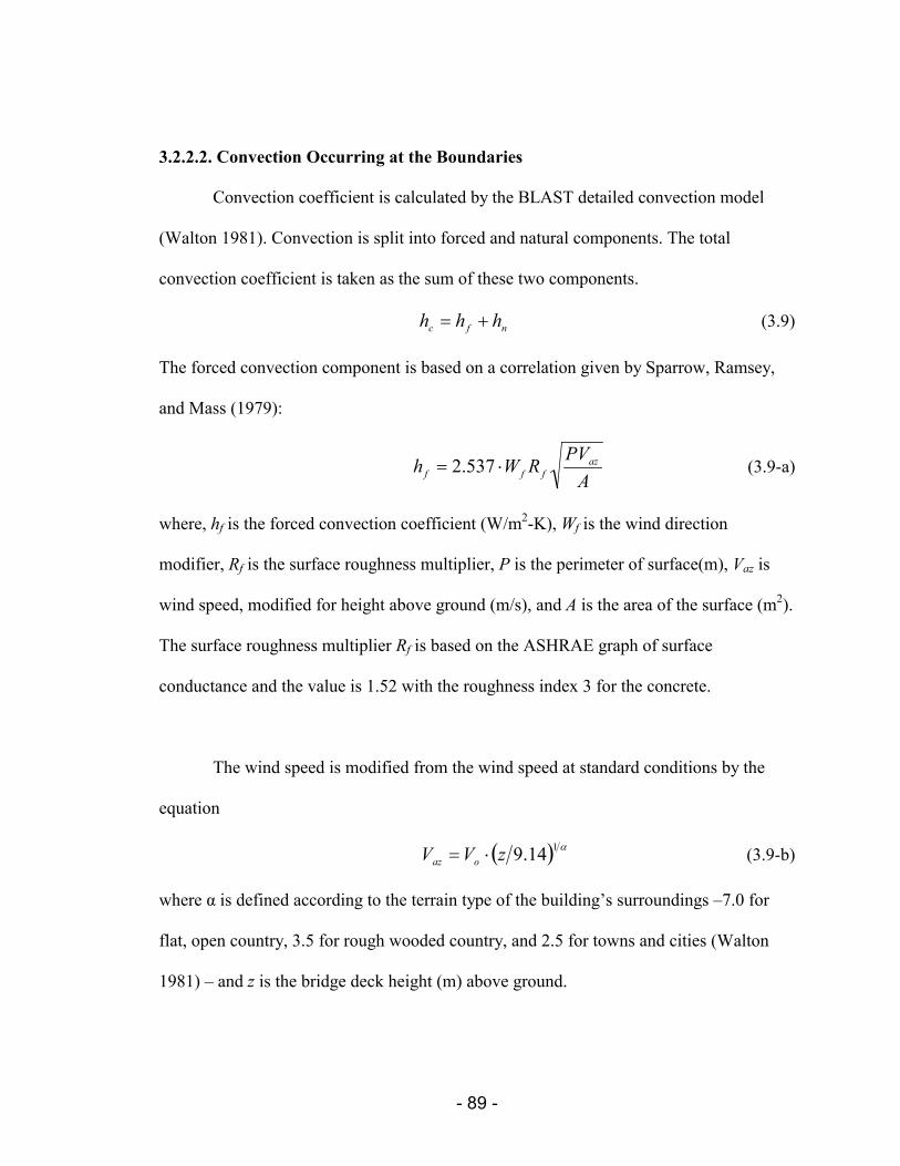
3.2.2.2. Convection Occurring at the Boundaries
Convection coefficient is calculated by the BLAST detailed convection model
(Walton 1981). Convection is split into forced and natural components. The total
convection coefficient is taken as the sum of these two components.
h (3.9) nfc hh ��
The forced convection component is based on a correlation given by Sparrow, Ramsey,
and Mass (1979):
A
PVRWh azfff �� 537.2 (3.9-a)
where, hf is the forced convection coefficient (W/m2-K), Wf is the wind direction
modifier, Rf is the surface roughness multiplier, P is the perimeter of surface(m), Vaz is
wind speed, modified for height above ground (m/s), and A is the area of the surface (m2).
The surface roughness multiplier Rf is based on the ASHRAE graph of surface
conductance and the value is 1.52 with the roughness index 3 for the concrete.
The wind speed is modified from the wind speed at standard conditions by the
equation
� � �114.9zVoaz ��V (3.9-b)
where α is defined according to the terrain type of the building’s surroundings –7.0 for
flat, open country, 3.5 for rough wooded country, and 2.5 for towns and cities (Walton
1981) – and z is the bridge deck height (m) above ground.
- 89 -
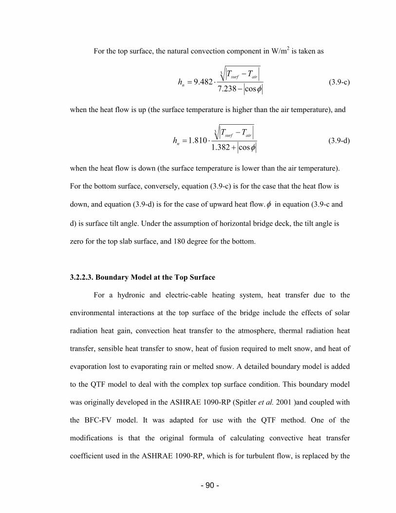
For the top surface, the natural convection component in W/m2 is taken as
�cos238.7
482.93
�
�
��
airsurf
n
TTh (3.9-c)
when the heat flow is up (the surface temperature is higher than the air temperature), and
�cos382.1
810.13
�
�
��
airsurf
n
TTh (3.9-d)
when the heat flow is down (the surface temperature is lower than the air temperature).
For the bottom surface, conversely, equation (3.9-c) is for the case that the heat flow is
down, and equation (3.9-d) is for the case of upward heat flow.� in equation (3.9-c and
d) is surface tilt angle. Under the assumption of horizontal bridge deck, the tilt angle is
zero for the top slab surface, and 180 degree for the bottom.
3.2.2.3. Boundary Model at the Top Surface
For a hydronic and electric-cable heating system, heat transfer due to the
environmental interactions at the top surface of the bridge include the effects of solar
radiation heat gain, convection heat transfer to the atmosphere, thermal radiation heat
transfer, sensible heat transfer to snow, heat of fusion required to melt snow, and heat of
evaporation lost to evaporating rain or melted snow. A detailed boundary model is added
to the QTF model to deal with the complex top surface condition. This boundary model
was originally developed in the ASHRAE 1090-RP (Spitler et al. 2001 )and coupled with
the BFC-FV model. It was adapted for use with the QTF method. One of the
modifications is that the original formula of calculating convective heat transfer
coefficient used in the ASHRAE 1090-RP, which is for turbulent flow, is replaced by the
- 90 -
method described in the previous section. Please refer to Chapter 1 for the details of the
ASHRAE 1090-RP boundary model for the top surface. In addition, solar radiation heat
gain has been added, and the long-wave radiation model has been modified as discussed
in the section 3.2.2.1.
The transfer function model is coupled to the boundary condition model by
passing surface temperature information and heat flux information between the two
models. Surface temperatures are required as inputs for the transfer function method. The
current time step’s temperatures are unknown – for each time step, a guess must be made
initially, then iterated on. The transfer function model passes the surface flux it has
calculated to the top and the bottom boundary condition models. The boundary condition
models then calculate the surface temperatures and the mass condition under these
surface flux inputs. The new surface temperatures are, in turn, passed back to the transfer
function model. This iterative process is considered converged when the surface
temperatures calculated by the boundary model become consistent with those used in the
transfer function model.
3.2.3. Heat Transfer at the Source Location
For slabs with the internal heat source, qsource, t, heat flux at the source location at
the current time t, is an input to calculate the current surface fluxes as Equation (3.1) and
(3.2). Different system control schemes start with different known conditions. In flux
control, the heat source is defined and the temperatures of the working fluid need to be
calculated. However, in temperature control, the control profile defines the inlet fluid
- 91 -

temperature. The heat flux at the source location needs to be calculated to satisfy the heat
balance between the heat loss of the fluid and the heat gain of the bridge material. That is,
(3.10) ,, tsourcetfluid qq �
It should be made clear that the source location refers to the outside tube wall that
directly has contact with concrete. Then, it assumes that the tube quickly reaches the heat
balance with the working fluid.
The transfer function for the calculation of Tsrc,t, the temperature at the source
location at time t, is in the form:
T (3.11) 1
1,1
,1
1,,1
1,,, �����
��
�
�
�
��
�
������
M
mmtsourcem
k
mmtsrcm
M
mmtomk
M
mmtimktsrc qwTfTyTx
This equation can be arranged to show the current source flux as a function of current
temperatures, past temperature and past source heat fluxes.
T
1
,2
1,1
,1
1,,1
1,,
, w
qwTfTyTxq
tsrc
M
mmtsourcem
k
mmtsrcm
M
mmtomk
M
mmtimk
tsource�
����
�
�����
��
�
�
�
��
�
��
(3.12)
That is, once the source temperature is known, the source flux can be determined by the
transfer function. The source flux then can be used to calculation the heat flows occurred
at the surfaces. Thus, the problem of calculating qsource, t in the temperature control
reduces to how to calculate the temperature at the source location (Tsrc,t).
To calculate the temperature at the outer pipe wall, which is also the temperature
at the source location for the QTF equations, the overall bridge deck system can be
thought of as a heat exchanger. Concrete can be taken as a stationary fluid with heat
- 92 -
exchange with the working fluid inside of the tube. (This is an approximation, but it
seems to be the best we can do.) Generally, there are two alternative heat exchanger
methodologies. It’s more convenient to use the effectiveness-NTU method in this case.
NTU algorithm for the calculation of the temperature at the source location
The effectiveness � is defined as:
maxqq
�� (3.13)
The actual heat transfer rate q can be obtained through the effectiveness and the
maximum possible heat transfer rate.
It’s assumed that the temperature along the outside tube wall in the calculation
domain is uniform. This assumption was made in the transfer functions calculation
(Strand 1995). The maximum heat transfer rate can be obtained if one of the fluids were
to undergo a temperature change equal to the maximum temperature difference present in
the exchange, which is the difference in the entering temperatures of the hot and cold
fluids. In this case, because the source is characterized by a single temperature, the
maximum temperature difference is the difference in the entering temperature of the hot
fluid and the source temperature. It limits the source temperature to be lower than the
outlet fluid temperature, which may not be true in actuality.
In the following section, the calculations of the effectiveness and the convective
heat transfer coefficient are explained. It’s followed by an explanation of the relation
- 93 -
between the source temperature and the fluid inlet and outlet temperatures. This is
summarized in the flow chart shown in Figure 3.2.
�� Effectiveness calculation
The effectiveness is related to the NTU (the number of transfer units) and
capacity ratio C, which can be found in any introductory heat transfer book.
minC
UANTU � (3.14)
max
min
CCC � (3.15)
Where � � � �� � � � � �� � max,min maxmin cm,cmC cm,cmconcretepfluidpconcretepfluidp ���� ��C .
The assumption of uniform temperature at the source location implies that “the
stationary fluid” undergoes a very small temperature difference. To satisfy the energy
balance between fluids, it infers that heat capacity of the concrete deck is much larger
than that for working fluid, which results in the capacity ratio C going to zero. In the case
that 0�C , the heat-exchanger effectiveness relation approaches a simple formula,
� (3.16) 1 NTUe�
��
� �
fluidpcmUANTU
�� (3.16-a)
where UA is the overall heat transfer coefficient between the fluid and the outer pipe
wall. With the consideration of the effect caused by the tubes, convection resistance Rconv
- 94 -
and the conductive resistance Rcond caused by pipe wall are presented in the overall heat
transfer coefficient, and UA is in term of the outer pipe area Ao.
1oA
RR condconv��UA (3.16-b)
dD
hAA
hR
i
oconv
11�� (3.16-c)
pipepipe
o
cond kdDD
LkdDA
R2
ln
2
ln ��
���
�
�
��
���
�
��
(3.16-d)
where h is the convection coefficient, Ai is the inside pipe area, kpipe is the conductivity of
tube, D is the tube outer diameter, d is the interior tube diameter and L is the tube length.
�� Convection heat transfer coefficient
As shown in equation (3.15-c), the convective heat transfer coefficient h is
required for NTU and effectiveness calculation. The convective heat transfer
coefficient can be obtained from internal flow correlations.
�
kdhNuD�
� (3.17)
where k is the thermal conductivity of the working fluid.
For laminar flow in a tube of constant surface temperature, the Nusselt number is
defined as a constant, 4.36. For the turbulent internal flow, the correlation given by
Gnielinski (1976) is used to determine the Nusselt number:
� �� �
� � � �
0.1Pr27.121Pr1000Re2
3221 f
fNu DD
��
�
� (3.18)
- 95 -
where Pr is the Prandtl number of the working fluid, f is the friction factor given by the
Eq(3.18-a), and ReD is the Reynolds number which is defines by equation (3.18-b).
� �� �
28.3Reln58.11
2 fD �
� (3.18-a)
4 d
mD
��
�
��
�Re (3.18-b)
where µ is the absolute viscosity of the working fluid. If the Reynolds number is greater
than 2300, the flow is taken as turbulent.
�� Relation between the source temperature and the fluid temperature
Through the definition of the effectiveness, a relation between the temperature at
the source location and fluid temperature can be established. First, the formula for the
heat balance on the fluid side is
q (3.19) )()( oifluidp TTcm �� �
where q is the heat transfer rate, and equals the heat transfer rate between the tube and the
concrete, m is the mass flow rate of the working fluid, c� p is the specific heat of the
working fluid, Ti is the inlet fluid temperature and To is the outlet fluid temperature. The
maximum amount of heat transfer that can occur is
q (3.20) )()(max srcifluidp TTcm �� �
where Tsrc is the current temperature at the source location. Substituting equation (3.19)
and equation (3.20) into the definition of the effectiveness, a relation between the source
temperature and the fluid temperature is established.
�
oiiSrc
TTT �
��T (3.21)
- 96 -
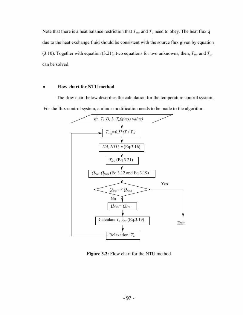
Note that there is a heat balance restriction that Tsrc and To need to obey. The heat flux q
due to the heat exchange fluid should be consistent with the source flux given by equation
(3.10). Together with equation (3.21), two equations for two unknowns, then, Tsrc and To,
can be solved.
�� Flow chart for NTU method
The flow chart below describes the calculation for the temperature control system.
For the flux control system, a minor modification needs to be made to the algorithm.
m�
Exit
Yes
Relaxation: To
Calculate To_New (Eq.3.19)
Qfluid= QSrc
QSrc,=? Qfluid
QSrc, Qfluid (Eq.3.12 and Eq.3.19)
TSrc (Eq.3.21)
UA, NTU, ε (Eq.3.16)
Tavg=0.5*(Ti+To)
, Ti, D, L. To(guess value)
No
Figure 3.2: Flow chart for the NTU method
- 97 -

3.3. Implementing in HVACSIM+ Environment
The following changes are made to make the transfer function model compatible
to HVACSIM+ environment (Clark, 1985):
�� Change the subroutine calling arguments of the models.
�� Assign the input variables and parameters, the values contained in XIN and PAR
arrays.
�� Save the variables required for the next time step.
�� Assign the output array, OUT to the output variables.
Once the necessary changes have been made to the model to make it compatible
with HVACSIM+, the next step is to install the model as a component model in the
component library. A description of the model must be added to the file TYPAR.DAT,
which is read by HVACGEN for creating the simulation work file.
The first line in TYPAR.DAT starts with an asterisk to indicate the beginning of a
new TYPE description. The second line contains the TYPE number, followed by a brief
description of the component. The third line contains information on the number of
SAVED variables, differential equations, inputs, outputs, and parameters respectively.
Next comes a set of lines describing the inputs, outputs and parameters.
Once the description has been added to the TYPAR.DAT listing, the model TYPE
routine is added to the “types.for” file of MODSIM and a CALL statement for the
subroutine is added to the subroutine SELECT. Now, the component model is ready to be
- 98 -
used for simulation. The TYPAR.DAT listing for the bridge deck model is included in
Appendix.
3.4. Results and Discussion
As stated in the previous section, the QTF model can calculate one-dimensional
or two-dimensional heat transfer depending on the transfer functions supplied to the
model. For one-dimensional problems, the model is tested by comparing simulation
results to analytical solutions. For two-dimensional problems, results are compared with
those from other simulation programs.
3.4.1. One Dimensional Comparative Studies
3.4.1.1.Comparison of Numerical and Analytical Solutions under No Heating
Conditions
Two tests, step change test and sinusoidal change test, have been conducted for
the surface response to changes in the air temperature under no flow conditions. The
numerical solution obtained using the QTF model in the HVACSim+ environment and
the analytical solutions obtained using the ASHRAE Analytical Test Suite (Spitler et al,
2001), have been compared. Both the numerical and analytical tests are carried out using
the same set of parameters described in the following sections. The thermo-physical
properties for material used in the tests have been tabulated below in Table 3.1.
- 99 -
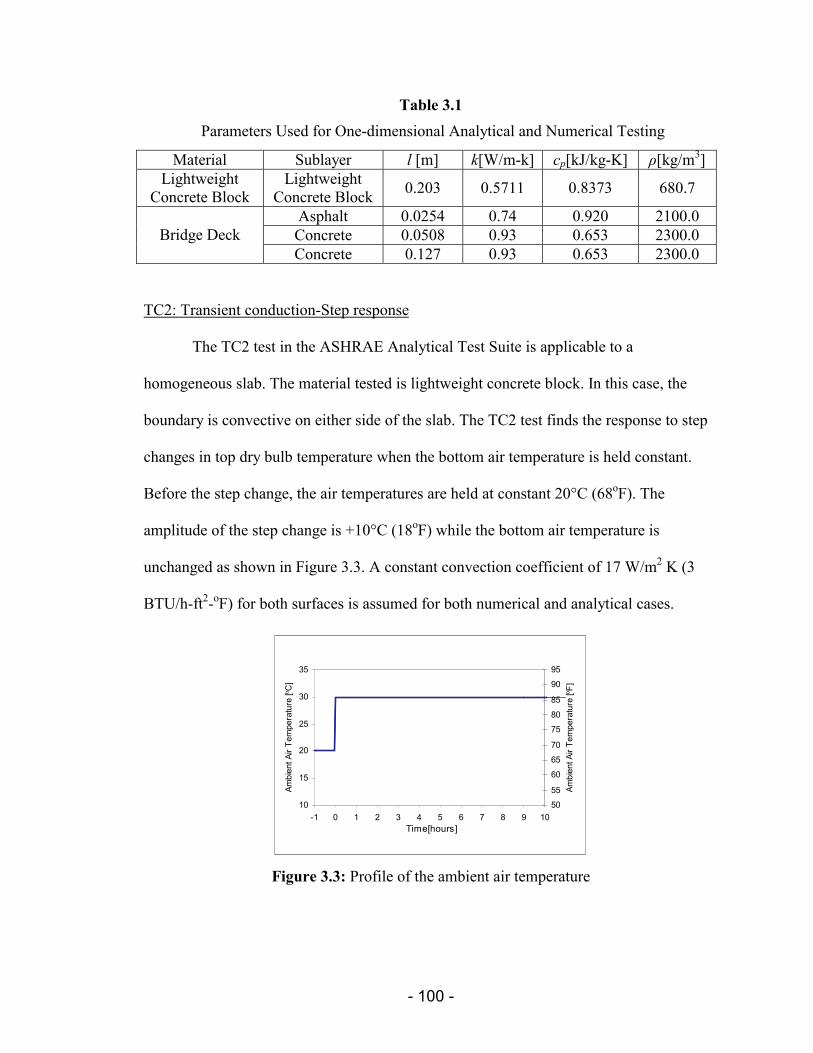
Table 3.1 Parameters Used for One-dimensional Analytical and Numerical Testing
Material Sublayer l [m] k[W/m-k] cp[kJ/kg-K] ρ[kg/m3] Lightweight
Concrete Block Lightweight
Concrete Block 0.203 0.5711 0.8373 680.7
Asphalt 0.0254 0.74 0.920 2100.0 Concrete 0.0508 0.93 0.653 2300.0 Bridge Deck Concrete 0.127 0.93 0.653 2300.0
TC2: Transient conduction-Step response
The TC2 test in the ASHRAE Analytical Test Suite is applicable to a
homogeneous slab. The material tested is lightweight concrete block. In this case, the
boundary is convective on either side of the slab. The TC2 test finds the response to step
changes in top dry bulb temperature when the bottom air temperature is held constant.
Before the step change, the air temperatures are held at constant 20°C (68oF). The
amplitude of the step change is +10°C (18oF) while the bottom air temperature is
unchanged as shown in Figure 3.3. A constant convection coefficient of 17 W/m2 K (3
BTU/h-ft2-oF) for both surfaces is assumed for both numerical and analytical cases.
10
15
20
25
30
35
-1 0 1 2 3 4 5 6 7 8 9 10Time[hours]
Ambi
ent A
ir Te
mpe
ratu
re [o C
]
50
55
60
65
70
75
80
85
90
95
Ambi
ent A
ir Te
mpe
ratu
re [o F
]
Figure 3.3: Profile of the ambient air temperature
- 100 -
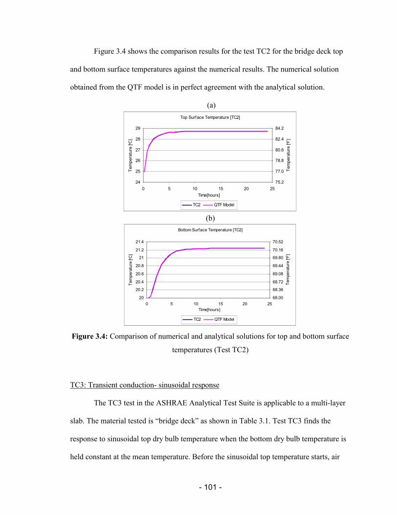
Figure 3.4 shows the comparison results for the test TC2 for the bridge deck top
and bottom surface temperatures against the numerical results. The numerical solution
obtained from the QTF model is in perfect agreement with the analytical solution.
(a) Top Surface Temperature [TC2]
24
25
26
27
28
29
0 5 10 15 20 25Time[hours]
Tem
pera
ture
[o C]
75.2
77.0
78.8
80.6
82.4
84.2
Tem
pera
ture
[o F]
TC2 QTF Model
(b) Bottom Surface Temperature [TC2]
20
20.2
20.4
20.6
20.8
21
21.2
21.4
0 5 10 15 20 25Time[hours]
Tem
pera
ture
[o C]
68.00
68.36
68.72
69.08
69.44
69.80
70.16
70.52
Tem
pera
ture
[o F]
TC2 QTF Model
Figure 3.4: Comparison of numerical and analytical solutions for top and bottom surface
temperatures (Test TC2)
TC3: Transient conduction- sinusoidal response
The TC3 test in the ASHRAE Analytical Test Suite is applicable to a multi-layer
slab. The material tested is “bridge deck” as shown in Table 3.1. Test TC3 finds the
response to sinusoidal top dry bulb temperature when the bottom dry bulb temperature is
held constant at the mean temperature. Before the sinusoidal top temperature starts, air
- 101 -
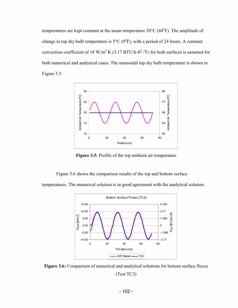
temperatures are kept constant at the mean temperature 20°C (68oF). The amplitude of
change in top dry bulb temperature is 5°C (9oF), with a period of 24 hours. A constant
convection coefficient of 18 W/m2 K (3.17 BTU/h-ft2-oF) for both surfaces is assumed for
both numerical and analytical cases. The sinusoidal top dry bulb temperature is shown in
Figure 3.5.
10
15
20
25
30
0 20 40 60 80
Time[hours]
Ambi
ent A
ir Te
mpe
ratu
re [o C
]
50
59
68
77
86
Ambi
ent A
ir Te
mpe
ratu
re [o F
]
Figure 3.5: Profile of the top ambient air temperature
Figure 3.6 shows the comparison results of the top and bottom surface
temperatures. The numerical solution is in good agreement with the analytical solution.
Bottom Surface Fluxes [TC3]
-10.00
-5.00
0.00
5.00
10.00
15.00
0 20 40 60 80
Time[hours]
Flux
[W/m
2 ]
-3.17
-1.585
0
1.585
3.17
4.755
Flux
[BTU
/hr-
ft2 ]
QTF Model TC3
Figure 3.6: Comparison of numerical and analytical solutions for bottom surface fluxes
(Test TC3)
- 102 -
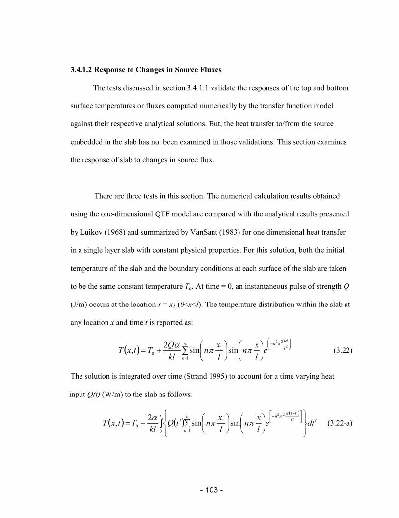
3.4.1.2 Response to Changes in Source Fluxes
The tests discussed in section 3.4.1.1 validate the responses of the top and bottom
surface temperatures or fluxes computed numerically by the transfer function model
against their respective analytical solutions. But, the heat transfer to/from the source
embedded in the slab has not been examined in those validations. This section examines
the response of slab to changes in source flux.
There are three tests in this section. The numerical calculation results obtained
using the one-dimensional QTF model are compared with the analytical results presented
by Luikov (1968) and summarized by VanSant (1983) for one dimensional heat transfer
in a single layer slab with constant physical properties. For this solution, both the initial
temperature of the slab and the boundary conditions at each surface of the slab are taken
to be the same constant temperature To. At time = 0, an instantaneous pulse of strength Q
(J/m) occurs at the location x = x1 (0<x<l). The temperature distribution within the slab at
any location x and time t is reported as:
� ����
����
���
��
���
���
���
��� �
222
sinsin2,1
10
l
tn
ne
lxn
lxn
klQTtxT
�
�
��
�
(3.22)
The solution is integrated over time (Strand 1995) to account for a time varying heat
input Q(t) (W/m) to the slab as follows:
� � � �� �
� � ���
���
��
���
��
�
��
����
�
�
��
���
� t
n
l
ttn
tdelxn
lxntQ
klTtxT
0 1
10
222
sinsin2,�
�
��
�
(3.22-a)
- 103 -
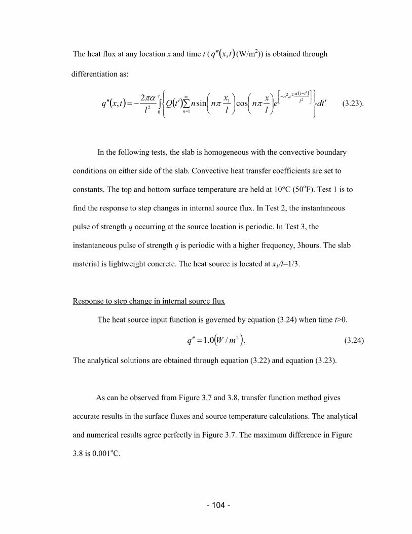
The heat flux at any location x and time t ( � �txq ,�� (W/m2)) is obtained through
differentiation as:
� � � �� �
� � ���
���
��
���
��
�
��
������
�
�
��
���
� t
n
l
ttn
tdelxn
lxnntQ
ltxq
0 1
12
222
cossin2,�
�
��
��
(3.23).
In the following tests, the slab is homogeneous with the convective boundary
conditions on either side of the slab. Convective heat transfer coefficients are set to
constants. The top and bottom surface temperature are held at 10°C (50oF). Test 1 is to
find the response to step changes in internal source flux. In Test 2, the instantaneous
pulse of strength q occurring at the source location is periodic. In Test 3, the
instantaneous pulse of strength q is periodic with a higher frequency, 3hours. The slab
material is lightweight concrete. The heat source is located at x1/l=1/3.
Response to step change in internal source flux
The heat source input function is governed by equation (3.24) when time t>0.
� �2/0.1 mW���q . (3.24)
The analytical solutions are obtained through equation (3.22) and equation (3.23).
As can be observed from Figure 3.7 and 3.8, transfer function method gives
accurate results in the surface fluxes and source temperature calculations. The analytical
and numerical results agree perfectly in Figure 3.7. The maximum difference in Figure
3.8 is 0.001oC.
- 104 -
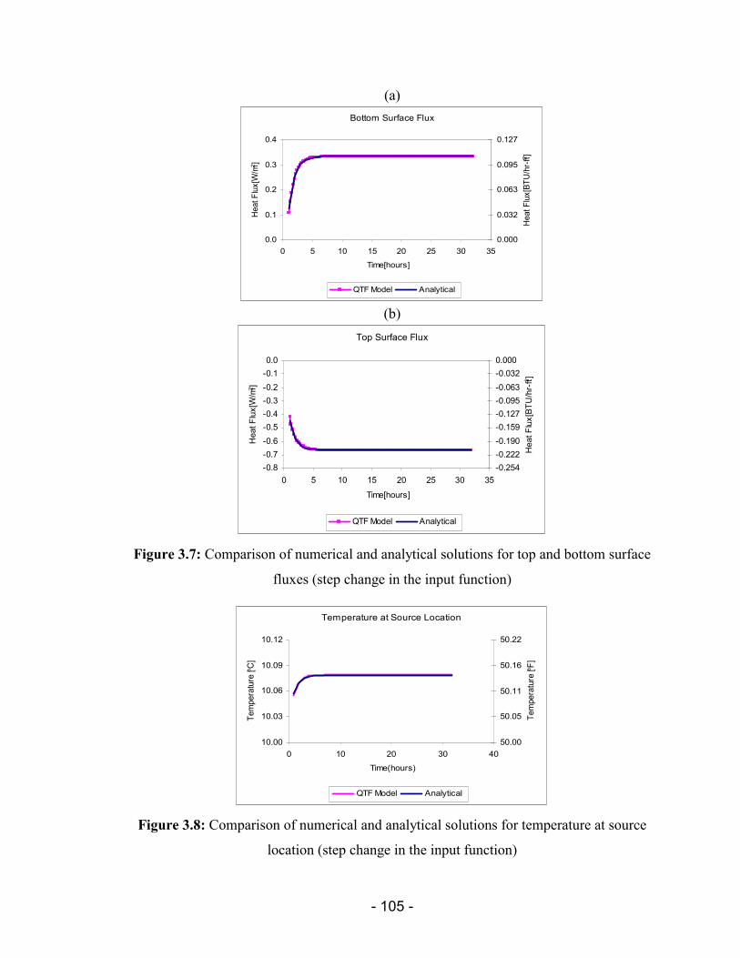
(a) Bottom Surface Flux
0.0
0.1
0.2
0.3
0.4
0 5 10 15 20 25 30 35
Time[hours]H
eat F
lux[
W/m
2 ]
0.000
0.032
0.063
0.095
0.127
Hea
t Flu
x[BT
U/h
r-ft2 ]
QTF Model Analytical
(b) Top Surface Flux
-0.8-0.7-0.6-0.5-0.4-0.3-0.2-0.10.0
0 5 10 15 20 25 30 35
Time[hours]
Hea
t Flu
x[W
/m2 ]
-0.254-0.222-0.190-0.159-0.127-0.095-0.063-0.0320.000
Hea
t Flu
x[BT
U/h
r-ft2 ]
QTF Model Analytical
Figure 3.7: Comparison of numerical and analytical solutions for top and bottom surface
fluxes (step change in the input function)
Temperature at Source Location
10.00
10.03
10.06
10.09
10.12
0 10 20 30 40
Time(hours)
Tem
pera
ture
[o C]
50.00
50.05
50.11
50.16
50.22
Tem
pera
ture
[o F]
QTF Model Analytical
Figure 3.8: Comparison of numerical and analytical solutions for temperature at source
location (step change in the input function)
- 105 -

Response to sinusoidal change in internal source flux
The heat source input function is governed by
� � � 2/ )242sin(0.10.1 mWtt �
���� �q (3.25)
where t is the hour in the simulation. The analytical solutions are obtained through
equation (3.22) and equation (3.23).
As can be seen from Figure 3.9, the transfer function method give accurate results in
surface flux calculation. In fact, the analytical and numerical results are indistinguishable
in Figure 3.9. The same indistinguishable trend can be observed from the source
temperature calculation as shown in Figure 3.10.
- 106 -
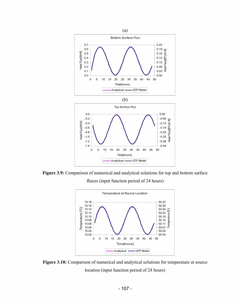
(a) Bottom Surface Flux
0.00.10.20.3
0.40.50.60.7
0 5 10 15 20 25 30 35 40 45 50
Time[hours]He
at F
lux[W
/m2 ]
0.000.030.060.10
0.130.160.190.22
Heat
Flux
[BTU
/h-ft2 ]
Analytical QTF Model
(b)
Top Surface Flux
-1.4-1.2
-1.0-0.8-0.6-0.4
-0.20.0
0 5 10 15 20 25 30 35 40 45 50
Time[hours]
Hea
t Flu
x[W
/m2 ]
-0.44-0.38
-0.32-0.25-0.19-0.13
-0.060.00
Hea
t Flux
[BTU
/h-ft2 ]
Analytical QTF Model
Figure 3.9: Comparison of numerical and analytical solutions for top and bottom surface
fluxes (input function period of 24 hours)
Temperature at Source Location
10.0010.0210.0410.0610.0810.1010.1210.1410.1610.18
0 5 10 15 20 25 30 35 40 45 50
Time[hours]
Tem
pera
ture
[o C]
50.0050.0450.0750.1150.1450.1850.2250.2550.2950.32
Tem
pera
ture
[o F]
Analytical QTF Model
Figure 3.10: Comparison of numerical and analytical solutions for temperature at source
location (input function period of 24 hours)
- 107 -
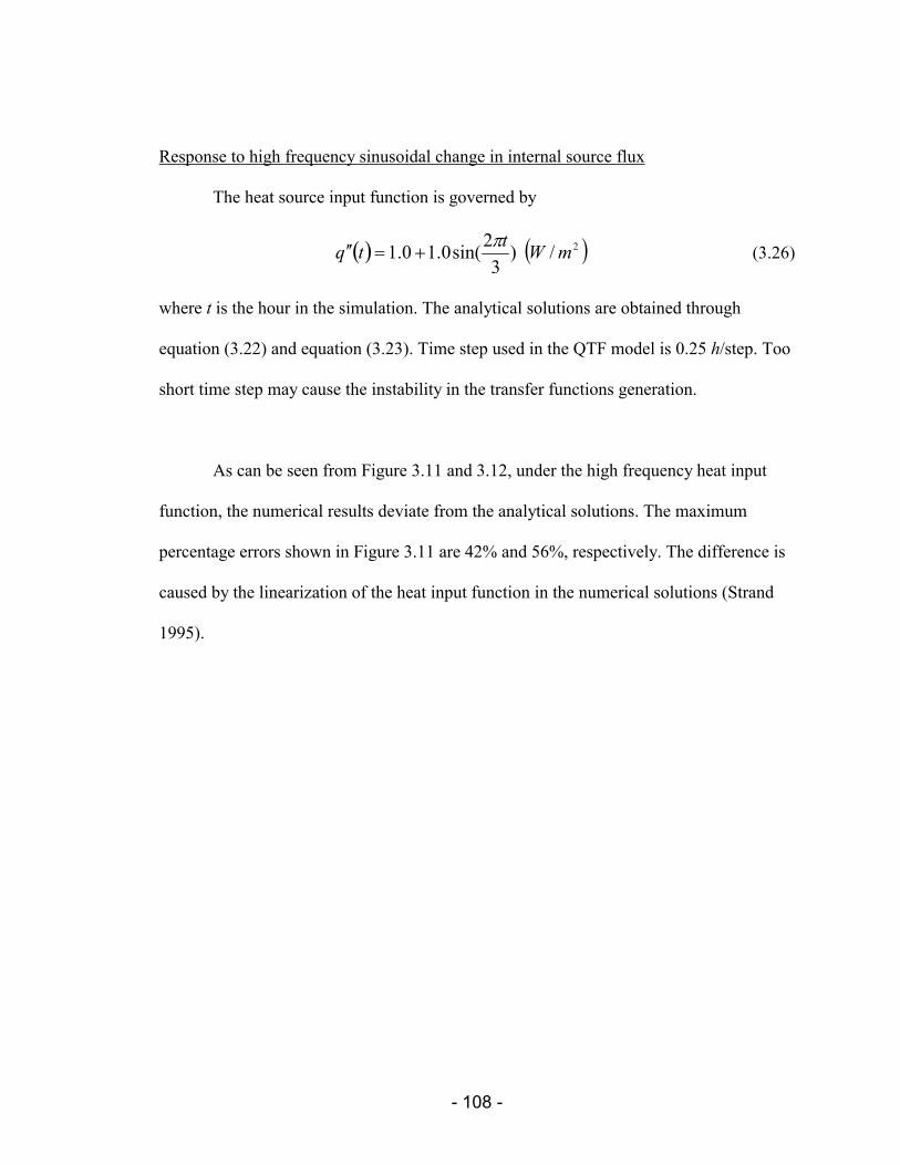
Response to high frequency sinusoidal change in internal source flux
The heat source input function is governed by
� � � 2/ )3
2sin(0.10.1 mWtt �
���� �q (3.26)
where t is the hour in the simulation. The analytical solutions are obtained through
equation (3.22) and equation (3.23). Time step used in the QTF model is 0.25 h/step. Too
short time step may cause the instability in the transfer functions generation.
As can be seen from Figure 3.11 and 3.12, under the high frequency heat input
function, the numerical results deviate from the analytical solutions. The maximum
percentage errors shown in Figure 3.11 are 42% and 56%, respectively. The difference is
caused by the linearization of the heat input function in the numerical solutions (Strand
1995).
- 108 -
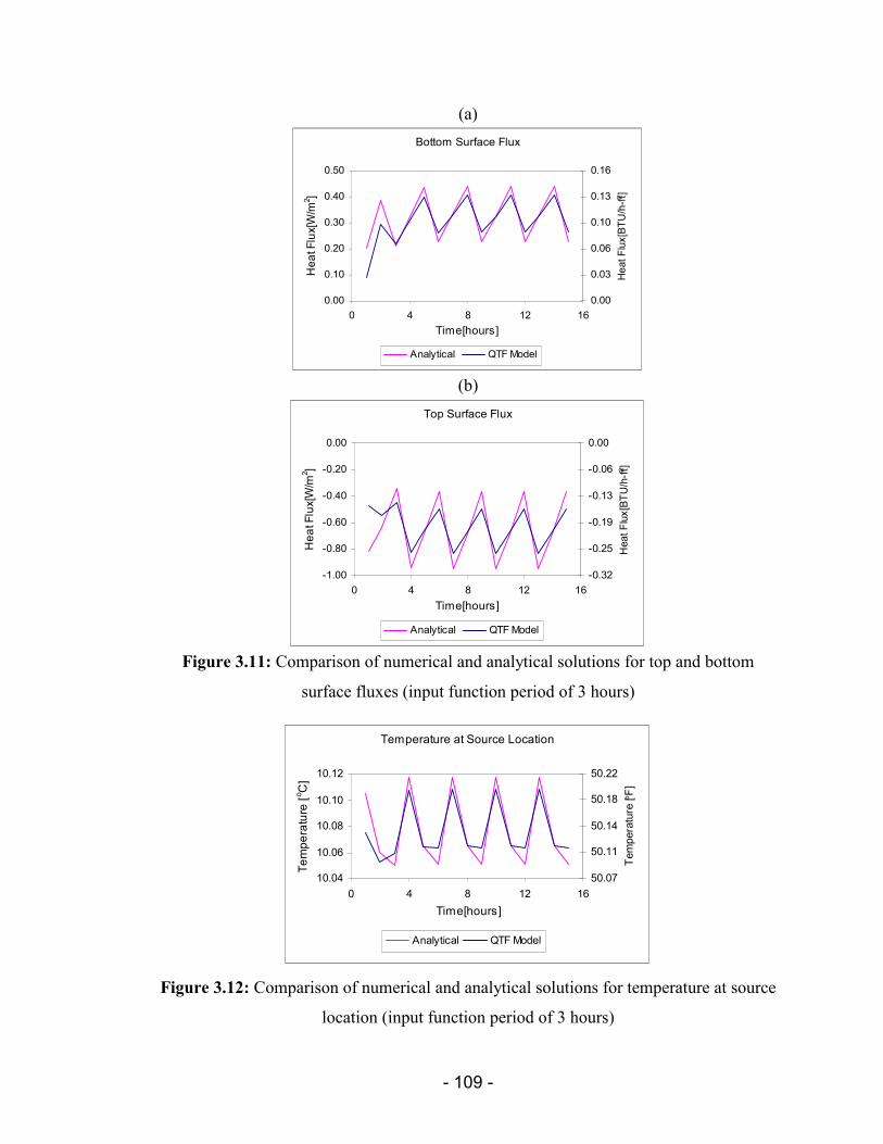
(a) Bottom Surface Flux
0.00
0.10
0.20
0.30
0.40
0.50
0 4 8 12 16Time[hours]
Hea
t Flu
x[W
/m2 ]
0.00
0.03
0.06
0.10
0.13
0.16
Hea
t Flu
x[BT
U/h
-ft2 ]
Analytical QTF Model
(b)
Top Surface Flux
-1.00
-0.80
-0.60
-0.40
-0.20
0.00
0 4 8 12 16Time[hours]
Hea
t Flu
x[W
/m2 ]
-0.32
-0.25
-0.19
-0.13
-0.06
0.00
Hea
t Flu
x[BT
U/h
-ft2 ]Analytical QTF Model
Figure 3.11: Comparison of numerical and analytical solutions for top and bottom
surface fluxes (input function period of 3 hours)
Temperature at Source Location
10.04
10.06
10.08
10.10
10.12
0 4 8 12 16Time[hours]
Tem
pera
ture
[o C]
50.07
50.11
50.14
50.18
50.22
Tem
pera
ture
[o F]
Analytical QTF Model
Figure 3.12: Comparison of numerical and analytical solutions for temperature at source
location (input function period of 3 hours)
- 109 -
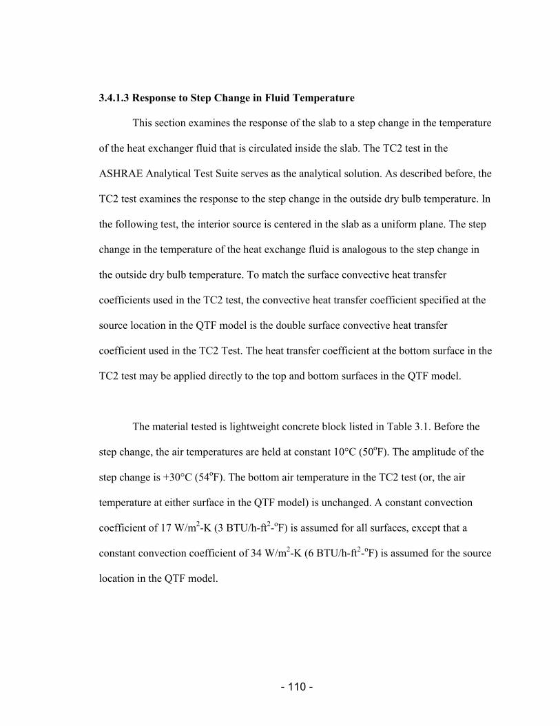
3.4.1.3 Response to Step Change in Fluid Temperature
This section examines the response of the slab to a step change in the temperature
of the heat exchanger fluid that is circulated inside the slab. The TC2 test in the
ASHRAE Analytical Test Suite serves as the analytical solution. As described before, the
TC2 test examines the response to the step change in the outside dry bulb temperature. In
the following test, the interior source is centered in the slab as a uniform plane. The step
change in the temperature of the heat exchange fluid is analogous to the step change in
the outside dry bulb temperature. To match the surface convective heat transfer
coefficients used in the TC2 test, the convective heat transfer coefficient specified at the
source location in the QTF model is the double surface convective heat transfer
coefficient used in the TC2 Test. The heat transfer coefficient at the bottom surface in the
TC2 test may be applied directly to the top and bottom surfaces in the QTF model.
The material tested is lightweight concrete block listed in Table 3.1. Before the
step change, the air temperatures are held at constant 10°C (50oF). The amplitude of the
step change is +30°C (54oF). The bottom air temperature in the TC2 test (or, the air
temperature at either surface in the QTF model) is unchanged. A constant convection
coefficient of 17 W/m2-K (3 BTU/h-ft2-oF) is assumed for all surfaces, except that a
constant convection coefficient of 34 W/m2-K (6 BTU/h-ft2-oF) is assumed for the source
location in the QTF model.
- 110 -
Figure 3.13 and 3.14 show the comparison results. The results from the QTF
model agree well with those from the TC2 test. Because of symmetry in the geometry and
boundary conditions supplied to the QTF model, the temperature distribution obtained
from the QTF model is symmetric, and the same surface temperatures are obtained for
both surfaces.
(a) Temperature at the Source Location
20.0022.0024.0026.0028.0030.0032.0034.0036.00
0 1 2 3 4 5 6 7 8 9 10
Time[hours]
Tem
pera
ture
[o C
]
68.0071.6075.2078.8082.4086.0089.6093.2096.80
Tem
pera
ture
[oF]
TC2 QTF
(b) Heat Flux at the Souce Location
0.00
50.00
100.00
150.00
200.00
250.00
0 1 2 3 4 5 6 7 8 9 10
Time[hours]
Hea
t Flu
x [W
/m2 ]
0.00
15.85
31.70
47.54
63.39
79.24
Hea
t Flu
x [B
TU/h
-ft2 ]
TC2 QTF
Figure 3.13: Comparison of numerical and analytical solutions for the temperature and
the heat flux at the source location
- 111 -
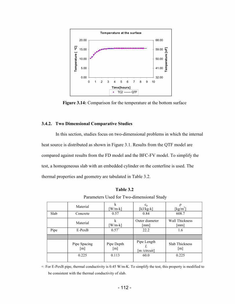
Temperature at the surface
0.00
5.00
10.00
15.00
20.00
0 1 2 3 4 5 6 7 8 9 10
Time[hours]
Tem
pera
ture
[o C
]32.00
41.00
50.00
59.00
68.00
Tem
pera
ture
[oF]
TC2 QTF
Figure 3.14: Comparison for the temperature at the bottom surface
3.4.2. Two Dimensional Comparative Studies
In this section, studies focus on two-dimensional problems in which the internal
heat source is distributed as shown in Figure 3.1. Results from the QTF model are
compared against results from the FD model and the BFC-FV model. To simplify the
test, a homogeneous slab with an embedded cylinder on the centerline is used. The
thermal properties and geometry are tabulated in Table 3.2.
Table 3.2 Parameters Used for Two-dimensional Study
Material k [W/m-k]
cp [kJ/kg-k]
ρ [kg/m3]
Slab Concrete 0.57 0.84 608.7
Material k [W/m-k]
Outer diameter [mm]
Wall Thickness [mm]
Pipe E-PexB 0.57+ 22.2 1.6
Pipe Spacing [m]
Pipe Depth [m]
Pipe Length L
[m /circuit]
Slab Thickness [m]
0.225 0.113 60.0 0.225
+: For E-PexB pipe, thermal conductivity is 0.45 W/m-K. To simplify the test, this property is modified to
be consistent with the thermal conductivity of slab.
- 112 -
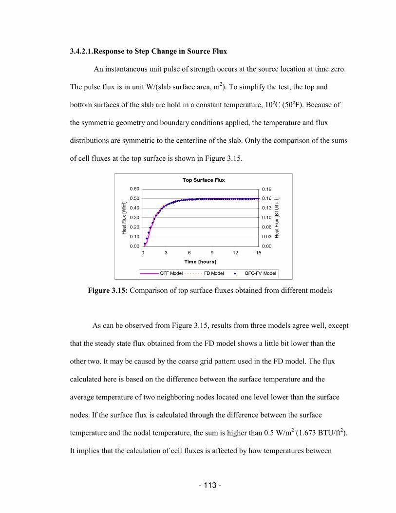
3.4.2.1.Response to Step Change in Source Flux
An instantaneous unit pulse of strength occurs at the source location at time zero.
The pulse flux is in unit W/(slab surface area, m2). To simplify the test, the top and
bottom surfaces of the slab are hold in a constant temperature, 10oC (50oF). Because of
the symmetric geometry and boundary conditions applied, the temperature and flux
distributions are symmetric to the centerline of the slab. Only the comparison of the sums
of cell fluxes at the top surface is shown in Figure 3.15.
Top Surface Flux
0.00
0.10
0.20
0.30
0.40
0.50
0.60
0 3 6 9 12 15
Time [hours]
Heat
Flux
[W/m
2 ]
0.00
0.03
0.06
0.10
0.13
0.16
0.19
Heat
Flux
[BTU
/h-ft2 ]
QTF Model FD Model BFC-FV Model
Figure 3.15: Comparison of top surface fluxes obtained from different models
As can be observed from Figure 3.15, results from three models agree well, except
that the steady state flux obtained from the FD model shows a little bit lower than the
other two. It may be caused by the coarse grid pattern used in the FD model. The flux
calculated here is based on the difference between the surface temperature and the
average temperature of two neighboring nodes located one level lower than the surface
nodes. If the surface flux is calculated through the difference between the surface
temperature and the nodal temperature, the sum is higher than 0.5 W/m2 (1.673 BTU/ft2).
It implies that the calculation of cell fluxes is affected by how temperatures between
- 113 -
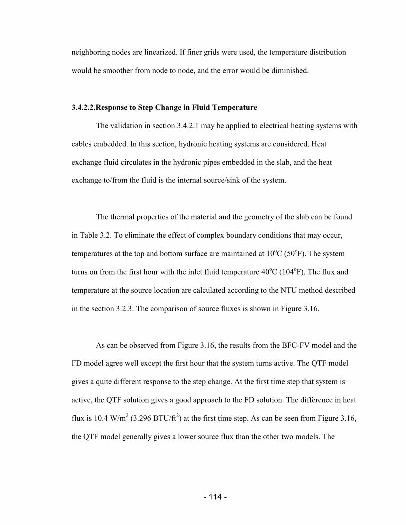
neighboring nodes are linearized. If finer grids were used, the temperature distribution
would be smoother from node to node, and the error would be diminished.
3.4.2.2.Response to Step Change in Fluid Temperature
The validation in section 3.4.2.1 may be applied to electrical heating systems with
cables embedded. In this section, hydronic heating systems are considered. Heat
exchange fluid circulates in the hydronic pipes embedded in the slab, and the heat
exchange to/from the fluid is the internal source/sink of the system.
The thermal properties of the material and the geometry of the slab can be found
in Table 3.2. To eliminate the effect of complex boundary conditions that may occur,
temperatures at the top and bottom surface are maintained at 10oC (50oF). The system
turns on from the first hour with the inlet fluid temperature 40oC (104oF). The flux and
temperature at the source location are calculated according to the NTU method described
in the section 3.2.3. The comparison of source fluxes is shown in Figure 3.16.
As can be observed from Figure 3.16, the results from the BFC-FV model and the
FD model agree well except the first hour that the system turns active. The QTF model
gives a quite different response to the step change. At the first time step that system is
active, the QTF solution gives a good approach to the FD solution. The difference in heat
flux is 10.4 W/m2 (3.296 BTU/ft2) at the first time step. As can be seen from Figure 3.16,
the QTF model generally gives a lower source flux than the other two models. The
- 114 -
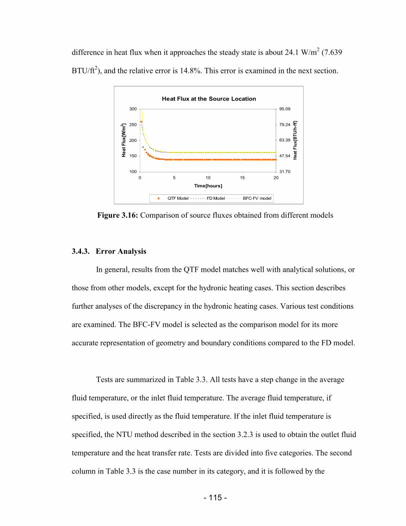
difference in heat flux when it approaches the steady state is about 24.1 W/m2 (7.639
BTU/ft2), and the relative error is 14.8%. This error is examined in the next section.
Heat Flux at the Source Location
100
150
200
250
300
0 5 10 15 20
Time[hours]
Heat
Flu
x[W
/m2 ]
31.70
47.54
63.39
79.24
95.09
Heat
Flu
x[BT
U/h-
ft2 ]
QTF Model FD Model BFC-FV model
Figure 3.16: Comparison of source fluxes obtained from different models
3.4.3. Error Analysis
In general, results from the QTF model matches well with analytical solutions, or
those from other models, except for the hydronic heating cases. This section describes
further analyses of the discrepancy in the hydronic heating cases. Various test conditions
are examined. The BFC-FV model is selected as the comparison model for its more
accurate representation of geometry and boundary conditions compared to the FD model.
Tests are summarized in Table 3.3. All tests have a step change in the average
fluid temperature, or the inlet fluid temperature. The average fluid temperature, if
specified, is used directly as the fluid temperature. If the inlet fluid temperature is
specified, the NTU method described in the section 3.2.3 is used to obtain the outlet fluid
temperature and the heat transfer rate. Tests are divided into five categories. The second
column in Table 3.3 is the case number in its category, and it is followed by the
- 115 -
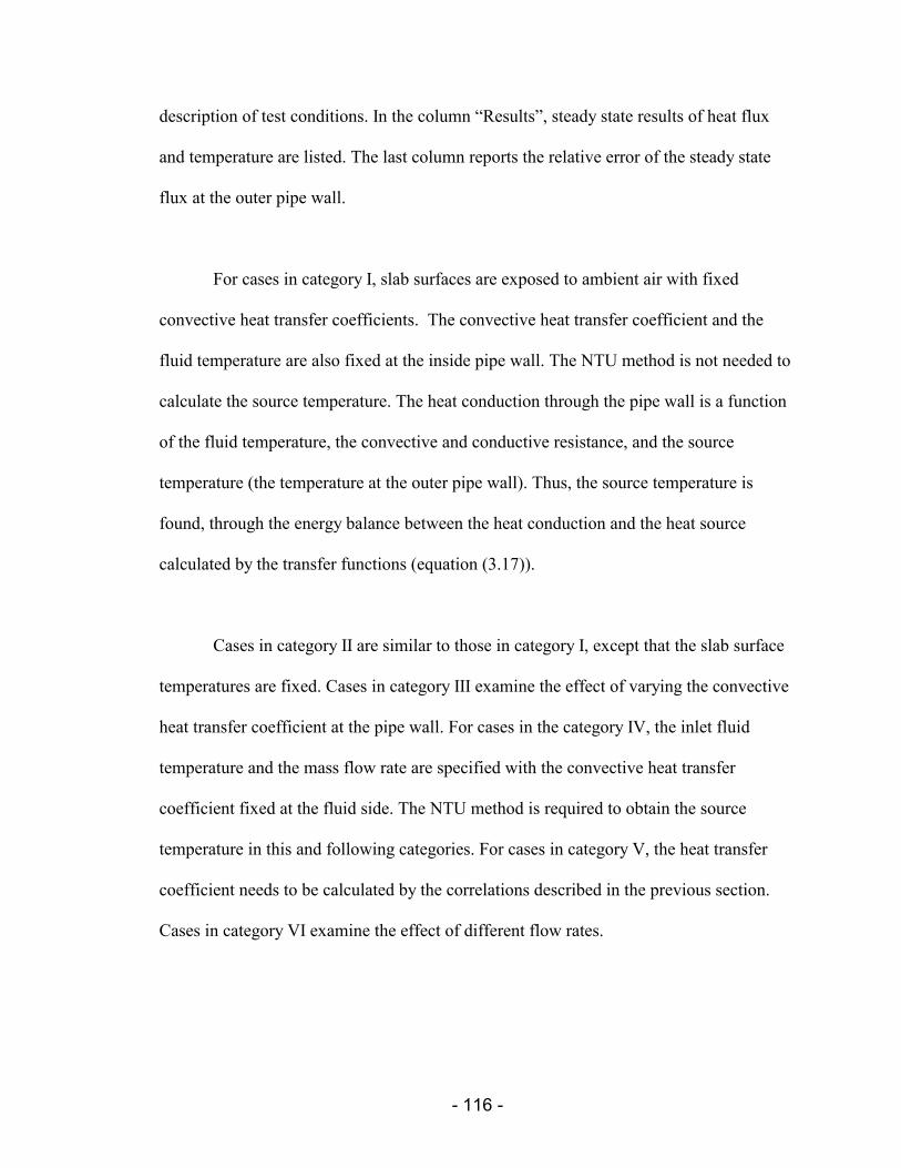
description of test conditions. In the column “Results”, steady state results of heat flux
and temperature are listed. The last column reports the relative error of the steady state
flux at the outer pipe wall.
For cases in category I, slab surfaces are exposed to ambient air with fixed
convective heat transfer coefficients. The convective heat transfer coefficient and the
fluid temperature are also fixed at the inside pipe wall. The NTU method is not needed to
calculate the source temperature. The heat conduction through the pipe wall is a function
of the fluid temperature, the convective and conductive resistance, and the source
temperature (the temperature at the outer pipe wall). Thus, the source temperature is
found, through the energy balance between the heat conduction and the heat source
calculated by the transfer functions (equation (3.17)).
Cases in category II are similar to those in category I, except that the slab surface
temperatures are fixed. Cases in category III examine the effect of varying the convective
heat transfer coefficient at the pipe wall. For cases in the category IV, the inlet fluid
temperature and the mass flow rate are specified with the convective heat transfer
coefficient fixed at the fluid side. The NTU method is required to obtain the source
temperature in this and following categories. For cases in category V, the heat transfer
coefficient needs to be calculated by the correlations described in the previous section.
Cases in category VI examine the effect of different flow rates.
- 116 -
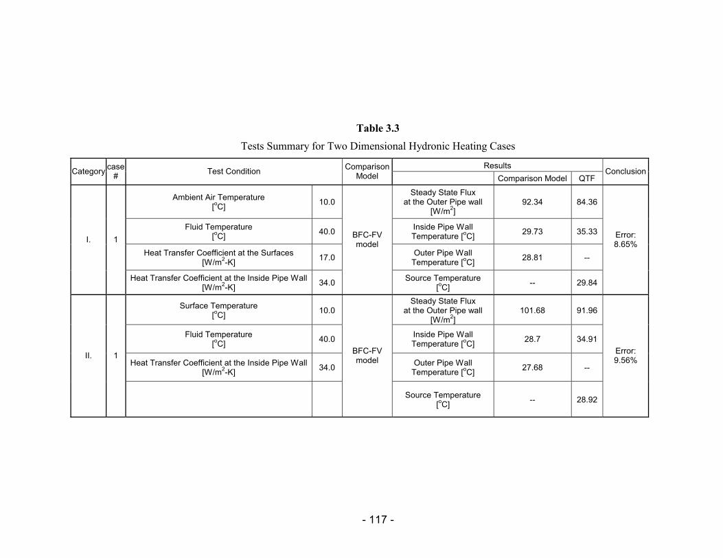
Table 3.3 Tests Summary for Two Dimensional Hydronic Heating Cases
Results Category case
# Test Condition ComparisonModel Comparison Model QTF
Conclusion
Ambient Air Temperature [oC] 10.0
Steady State Flux at the Outer Pipe wall
[W/m2] 92.34 84.36
Fluid Temperature [oC] 40.0 Inside Pipe Wall
Temperature [oC] 29.73 35.33
Heat Transfer Coefficient at the Surfaces [W/m2-K] 17.0 Outer Pipe Wall
Temperature [oC] 28.81 --
I.
1
Heat Transfer Coefficient at the Inside Pipe Wall [W/m2-K] 34.0
BFC-FV model
Source Temperature [oC] -- 29.84
Error: 8.65%
Surface Temperature [oC] 10.0
Steady State Flux at the Outer Pipe wall
[W/m2] 101.68 91.96
Fluid Temperature [oC] 40.0 Inside Pipe Wall
Temperature [oC] 28.7 34.91
Heat Transfer Coefficient at the Inside Pipe Wall [W/m2-K] 34.0 Outer Pipe Wall
Temperature [oC] 27.68 --II.
1
BFC-FV model
Source Temperature [oC] -- 28.92
Error: 9.56%
- 117 -
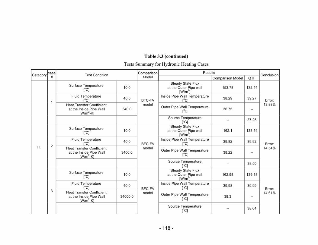
Table 3.3 (continued) Tests Summary for Hydronic Heating Cases
Results Category case # Test Condition Comparison
Model Comparison Model QTF Conclusion
Surface Temperature [oC] 10.0
Steady State Flux at the Outer Pipe wall
[W/m2] 153.78 132.44
Fluid Temperature [oC] 40.0 Inside Pipe Wall Temperature
[oC] 38.29 39.27
Heat Transfer Coefficient at the Inside Pipe Wall
[W/m2-K] 340.0 Outer Pipe Wall Temperature
[oC] 36.75 --
1
BFC-FV model
Source Temperature [oC] -- 37.25
Error: 13.88%
Surface Temperature [oC] 10.0
Steady State Flux at the Outer Pipe wall
[W/m2] 162.1 138.54
Fluid Temperature [oC] 40.0 Inside Pipe Wall Temperature
[oC] 39.82 39.92
Heat Transfer Coefficient at the Inside Pipe Wall
[W/m2-K] 3400.0 Outer Pipe Wall Temperature
[oC] 38.22 --
2
BFC-FV model
Source Temperature [oC] -- 38.50
Error: 14.54%
Surface Temperature [oC] 10.0
Steady State Flux at the Outer Pipe wall
[W/m2] 162.98 139.18
Fluid Temperature [oC] 40.0 Inside Pipe Wall Temperature
[oC] 39.98 39.99
Heat Transfer Coefficient at the Inside Pipe Wall
[W/m2-K] 34000.0 Outer Pipe Wall Temperature
[oC] 38.3 --
III.
3
BFC-FV model
Source Temperature [oC] -- 38.64
Error: 14.61%
- 118 -
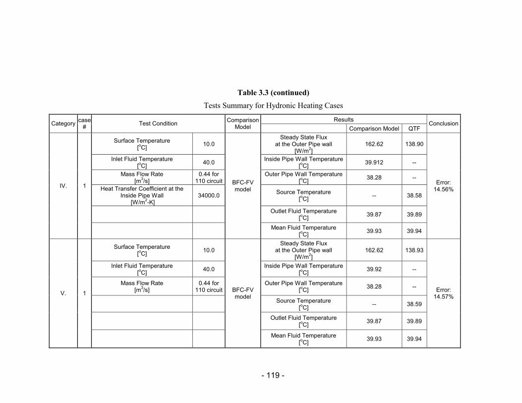
Table 3.3 (continued) Tests Summary for Hydronic Heating Cases
Results Category case # Test Condition Comparison
Model Comparison Model QTF Conclusion
Surface Temperature [oC] 10.0
Steady State Flux at the Outer Pipe wall
[W/m2] 162.62 138.90
Inlet Fluid Temperature [oC] 40.0 Inside Pipe Wall Temperature
[oC] 39.912 --
Mass Flow Rate [m3/s]
0.44 for 110 circuit
Outer Pipe Wall Temperature [oC] 38.28 --
Heat Transfer Coefficient at the Inside Pipe Wall
[W/m2-K] 34000.0 Source Temperature
[oC] -- 38.58
Outlet Fluid Temperature [oC] 39.87 39.89
IV.
1
BFC-FV model
Mean Fluid Temperature [oC] 39.93 39.94
Error: 14.56%
Surface Temperature [oC] 10.0
Steady State Flux at the Outer Pipe wall
[W/m2] 162.62 138.93
Inlet Fluid Temperature [oC] 40.0 Inside Pipe Wall Temperature
[oC] 39.92 --
Mass Flow Rate [m3/s]
0.44 for 110 circuit
Outer Pipe Wall Temperature [oC] 38.28 --
Source Temperature [oC] -- 38.59
Outlet Fluid Temperature [oC] 39.87 39.89
V.
1
BFC-FV model
Mean Fluid Temperature [oC] 39.93 39.94
Error: 14.57%
- 119 -
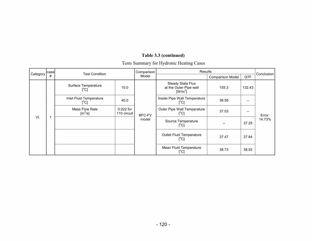
Table 3.3 (continued) Tests Summary for Hydronic Heating Cases
Results Category case
# Test Condition Comparison Model Comparison Model QTF
Conclusion
Surface Temperature [oC] 10.0
Steady State Flux at the Outer Pipe wall
[W/m2] 155.3 132.43
Inlet Fluid Temperature [oC] 40.0 Inside Pipe Wall Temperature
[oC] 38.58 --
Mass Flow Rate [m3/s]
0.022 for 110 circuit
Outer Pipe Wall Temperature [oC] 37.03 --
Source Temperature [oC] -- 37.25
Outlet Fluid Temperature [oC] 37.47 37.84
VI.
1
BFC-FV model
Mean Fluid Temperature [oC] 38.73 38.92
Error: 14.73%
- 120 -
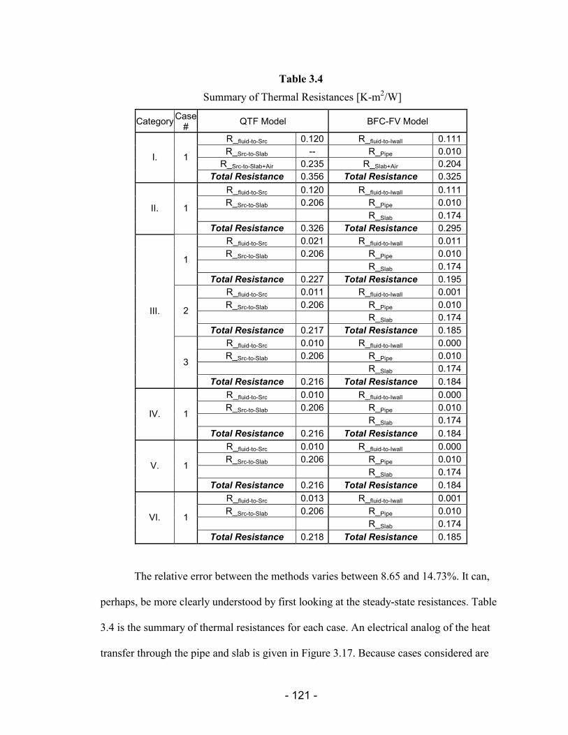
Table 3.4 Summary of Thermal Resistances [K-m2/W]
Category Case # QTF Model BFC-FV Model
R_fluid-to-Src 0.120 R_fluid-to-Iwall 0.111 R_Src-to-Slab -- R_Pipe 0.010
R_Src-to-Slab+Air 0.235 R_Slab+Air 0.204 I. 1
Total Resistance 0.356 Total Resistance 0.325 R_fluid-to-Src 0.120 R_fluid-to-Iwall 0.111 R_Src-to-Slab 0.206 R_Pipe 0.010
R_Slab 0.174 II. 1
Total Resistance 0.326 Total Resistance 0.295 R_fluid-to-Src 0.021 R_fluid-to-Iwall 0.011 R_Src-to-Slab 0.206 R_Pipe 0.010
R_Slab 0.174 1
Total Resistance 0.227 Total Resistance 0.195 R_fluid-to-Src 0.011 R_fluid-to-Iwall 0.001 R_Src-to-Slab 0.206 R_Pipe 0.010
R_Slab 0.174 2
Total Resistance 0.217 Total Resistance 0.185 R_fluid-to-Src 0.010 R_fluid-to-Iwall 0.000 R_Src-to-Slab 0.206 R_Pipe 0.010
R_Slab 0.174
III.
3
Total Resistance 0.216 Total Resistance 0.184 R_fluid-to-Src 0.010 R_fluid-to-Iwall 0.000 R_Src-to-Slab 0.206 R_Pipe 0.010
R_Slab 0.174 IV. 1
Total Resistance 0.216 Total Resistance 0.184 R_fluid-to-Src 0.010 R_fluid-to-Iwall 0.000 R_Src-to-Slab 0.206 R_Pipe 0.010
R_Slab V. 1
Total Resistance 0.216 Total Resistance 0.184 R_fluid-to-Src 0.013 R_fluid-to-Iwall 0.001 R_Src-to-Slab 0.206 R_Pipe 0.010
R_Slab 0.174 VI. 1
Total Resistance 0.218 Total Resistance 0.185
0.174
The relative error between the methods varies between 8.65 and 14.73%. It can,
perhaps, be more clearly understood by first looking at the steady-state resistances. Table
3.4 is the summary of thermal resistances for each case. An electrical analog of the heat
transfer through the pipe and slab is given in Figure 3.17. Because cases considered are
- 121 -
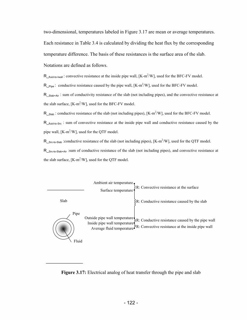
two-dimensional, temperatures labeled in Figure 3.17 are mean or average temperatures.
Each resistance in Table 3.4 is calculated by dividing the heat flux by the corresponding
temperature difference. The basis of these resistances is the surface area of the slab.
Notations are defined as follows.
R_fluid-to-Iwall : convective resistance at the inside pipe wall, [K-m2/W], used for the BFC-FV model.
R_Pipe : conductive resistance caused by the pipe wall, [K-m2/W], used for the BFC-FV model.
R_Slab+Air : sum of conductivity resistance of the slab (not including pipes), and the convective resistance at
the slab surface, [K-m2/W], used for the BFC-FV model.
R_Slab : conductive resistance of the slab (not including pipes), [K-m2/W], used for the BFC-FV model.
R_fluid-to-Src : sum of convective resistance at the inside pipe wall and conductive resistance caused by the
pipe wall, [K-m2/W], used for the QTF model.
R_Src-to-Slab :conductive resistance of the slab (not including pipes), [K-m2/W], used for the QTF model.
R_Src-to-Slab+Air :sum of conductive resistance of the slab (not including pipes), and convective resistance at
the slab surface, [K-m2/W], used for the QTF model.
R: Conductive resistance caused by the slab
R: Convective resistance at the surface
Slab
Fluid
Pipe Outside pipe wall temperature
Inside pipe wall temperatureAverage fluid temperature
Surface temperature
Ambient air temperature
R: Convective resistance at the inside pipe wall R: Conductive resistance caused by the pipe wall
Figure 3.17: Electrical analog of heat transfer through the pipe and slab
- 122 -
For each case, R_fluid-to-Src from the QTF model, which is the sum of convective
resistance at the inside pipe wall and the conductive resistance caused by the pipe wall,
almost exactly matches the sum of R_fluid-to-Iwall and R_Pipe obtained from the BFC-FV
model. It demonstrates the accurate calculation of the heat transfer between the fluid and
the outer pipe wall. However, as can be seen in category I, there is nearly a 15%
discrepancy between R_Src-to-Slab+Air and R_Slab. These should match exactly. Also, as can be
observed from category II to VI in Table 3.4, the conductive resistances (R_Src-to-Slab and
R_Slab) differ in the two models, with 0.206 (K-m2/W) (1.170 F-ft2/BTU) for the QTF
model and 0.174 (K-m2/W) (0.988 F-ft2/BTU) for the BFC-FV model. In the QTF model,
the resistance is set by the transfer functions developed by the QTF calculator. It implies
there are inaccuracies in the transfer functions generation.
In an attempt to reduce the errors, the tests were repeated using transfer functions
generated with a more refined internal grid. However, these transfer functions did not
improve the calculation. Another possible explanation of the error is the way in which the
two-dimensional geometry is interpreted in the "QTF calculator". In the "QTF
calculator", the pipe diameter is not required as an input for the two-dimensional
problem. The source is defined between two layers, which are measured from the slab
surfaces to the center of the pipe. The mixed geometry problem in this kind of system has
not been described accurately. Also, other causes may be possible, such as mathematical
calculation related to the matrix inverse and root finding.
- 123 -
The error of the conduction resistance is fixed once the material is selected for
simulations. The different relative error shown in Table 3.3 can be explained by the
relative importance of the conduction resistance error in the total resistance. For instance,
cases in category I have lower relative error compared to other tests, because with the
consideration of the convective resistance at the slab surface, the total resistance is
higher, and it makes the conductive resistance error less important, and so gives a lower
relative error. For cases in category III, with increasing convective heat transfer
coefficient at the fluid side, the convective resistance becomes lower and lower, and it
leads to lower total resistance and higher relative error as shown in Table 3.3 and 3.4.
Another point to be noticed is the effect of the convective heat transfer coefficient
in the fluid side. As can be observed from cases in category III, the relative error doesn’t
change much once the convective heat transfer coefficient at the inside pipe wall is over
3400 [W/m2-K]. It implies that the convective resistance diminishes and becomes
negligible as the flow rate increases. This can be observed directly from cases in category
V and VI.
One possible way to check the accuracy of the NTU method used in the
calculation of the source temperature and heat flux is the comparison between Case 3 in
Category III and Case 1 in Category IV. One difference in test conditions is that the
former specifies the fluid temperature and the latter sets the inlet fluid temperature. Then,
for the Case 1 in Category IV, the NTU method is used to obtain the outlet fluid
temperature and the heat transfer rate at the outer pipe wall. A large flow rate is used in
- 124 -
Category IV to make the average fluid temperature close to the fluid temperature for Case
3 in Category III. The relative error for these two cases are close as can be seen from
Table 3.3. This example implies the NTU method doesn’t impose extra error in the
simulation.
3.5. Summary
A design and simulation tool for modeling the performance of a bridge deck
heating system has been developed. The model (the QTF model) has been developed
based on the transfer function method. According to the transfer functions provided, the
model can solve the slab heat transfer problem for one-dimensional or two-dimensional
geometry.
For applications that can be considered as one-dimensional, the QTF model
presents accurate solutions as compared with analytical solutions from the literature and
the ASHRAE Analytical Test Suite. For applications considered as two-dimensional,
such as heat sources at discrete intervals, the results obtained from the QTF model match
well with those from the FD model and the BFC-FV model in the case of the fixed heat
flux input at the source location. However, in the case of hydronic heating systems with
heat exchange fluid circulated in the embedded pipe, the discrepancy is obvious. The
steady state flux obtained from the QTF model is always lower than results provided by
other models. This has been shown to be caused by inaccuracies in the transfer functions
provided by the QTF calculator.
- 125 -

Further research is suggested in the following areas:
�� A more accurate transfer function calculator is desirable.
�� Optimization of the source temperature calculation. Several methods may be tried
besides the currently used NTU method.
�� Additional validation of the model, using data collected under a wider range of
weather conditions (i.e. rain, snow, and ice conditions), would be useful. A
preliminary investigation is reported in the next chapter.
- 126 -
4. Validation of the QTF Model by Experimental Data
4.1. Introduction
The previous chapter describes the development of a new bridge deck model (the
QTF model) based on the time series method, and the model is validated through
analytical solutions and model comparisons. The work described in this chapter is to
validate the model by experimental data.
The QTF model depicting the OSU bridge deck system is simulated for heating
and recharge cases. A detailed description of the bridge deck system is given in the next
section. Experimentally measured inlet fluid temperature and mass flow rate are used as
inputs in simulations. For the recharge case, comparisons of top surface temperatures,
exit fluid temperatures, and heat transfer rate are given. For the heating case, results are
compared to the experimental measurements of the surface temperature and the exit fluid
temperature. This study is intended for establishing a better understanding of the
performance of the QTF model in simulations with real parameters and weather
conditions.
4.2. Previous Work
Continuous work and studies on transient simulations of hydronic heating systems
have been done in Oklahoma State University by using the finite difference bridge deck
model developed by Chiasson (2000).
- 127 -
Ramamoorthy (2001) discussed the performance of a hydronically heated bridge
deck system that is heated with a hybrid ground source heat pump system. The system is
simulated and the performance studied in detail for a sample bridge deck located at
Weatherford, OK. The simulation results for a few summer recharge set point
temperatures are presented. The advantages of using the bridge deck during summer for
recharging the ground is quite evident from simulation results. Storing the heat extracted
from bridge deck surface during summer raises the ground temperature, and makes it
available for use in winter for bridge deck heating. The study also shows that the system
modeling and simulation approach is a powerful tool to study and analyze the system
performance of several possible designs. Bridge deck heating systems have high initial
cost; their optimal design and operation is of paramount importance. Using the system
simulation approach, the performance of such systems and different control strategies
could be easily simulated and analyzed, and a cost efficient design solution can be
achieved.
Ongoing research at Oklahoma State University focuses on the development of a
bridge deck heating system to eliminate preferential icing. The heating system is
hydronic, and makes use of a ground source heat pump system, which recovers energy
stored in the earth, and uses it to heat the fluid circulated through the bridge deck. The
heating system automatically makes use of local and remote weather stations to forecast
potential icing conditions. The automatic nature of the controls has given rise to the
informal name "Smart Bridge". Initial research was done on a test bridge deck, which is
described in more detail in the following section, along with an experimentally calibrated
- 128 -
numerical model. Several critical parameters have been more carefully measured
(Progress Report, OSU Geothermal Smart Bridge, 2001). For instance, the measured
density of the sample concrete was 2324 kg/m3 at moisture content of 24% of total
saturation, and the density from oven-dry to saturated condition varies about 6%. The
thermal properties of the bridge deck were recomputed, taking into account two factors –
the double-T thermal mass and the rebar embedded in the bridge deck. As a first order
approximation, the double-T thermal mass was treated as a uniform layer of concrete 3.8
inches (97 mm thick). The rebar was accounted for by mass weighting the conductivity,
specific heat and density. The resulting simulations match the experimental results more
closely.
The following section describes the bridge deck system under investigation, the
weather data source, and experimental data used in the model validation.
�� OSU Bridge System
The experimental bridge heating system comprises a bridge deck with embedded
heat exchanger pipe loops, a single water-to-water heat pump, a six-borehole vertical
ground loop heat exchanger, along with circulating pumps and control system.
The experimental bridge deck is 18.3m (60 ft) long by 6.1m (20 ft) wide, but only
half (9.2m*6.1m) is heated. Bridge deck thickness is 0.254m (10 inch). The pipe work
consists of 10 fluid circuits laid in a serpentine configuration perpendicular to traffic flow
on the bridge. E-PexB Pipe from WattsHeatway is embedded. Nominal pipe diameters
are commonly 19.05mm (0.75 inch). The tubing is 0.0762m (3 inch) beneath the bridge
surface measured from the surface to the pipe center with pipe spacing of 0.3048m (1 ft).
- 129 -
The specific heat of concrete used in the simulation is 889 J/kg-K, and the density is 2474
kg/m3.
The vertical closed-loop ground source heat exchanger installation is comprised
of 6 boreholes with a diameter of 0.13 m (5.25 in) that are in a 2 by 3 configuration with
7.62 m (25 ft) spacing. Each borehole contains an HDPE U-bend pipe loop with nominal
diameter of 25 mm (1 in), and is grouted with a mixture of 4020 sand and bentonite.
The nominal cooling capacity of water-to-water heat pump used in the system is
35 KW (10 tons) with the design output temperature of the fluid in the range 38-55oC
(100-130oF). The working fluid is a mixture of water and propylene glycol, and
circulated at a rate of approximately 1.3 l/s (21 GPM) through the ground-loop system.
The bridge anti-icing system has initially been operated with on-off control of the
heating system. The objective has been to maintain the bridge surface temperature in the
range of 4.4-5.5oC in case of risk of icing or snowfall. In recharge mode, it is switched on
when the surface temperature is higher than 32.2oC (90oF) and switched off when the
temperature falls to 31.1oC (88oF).
�� Weather Data
The Oklahoma Mesonet is a collaborative project between Oklahoma State
University and the University of Oklahoma. The Mesonet is a network of 114 weather
stations distributed throughout Oklahoma. The measurements are packaged into
"observations" every 5 minutes, then the observations are transmitted to a central facility
every 15 minutes, 24 hours per day year-round. Nearly real-time weather data is
available to customers, including schools, over the internet. The Stillwater Mesonet
- 130 -

Station is about 1 mile from the medium-scale heated bridge deck. Its data is assumed as
same as that at the experimental site.
Weather data is rearranged and contained in a boundary variable file for
simulations in the HVACSim+ environment. The data set has information about solar
radiation, dry-bulb and dew point temperatures, precipitation, weather indicator, wind
speed, and solar angle. The sky temperature required for the system simulation is
calculated using the available weather data.
�� Experimental data
Experimental measurements of mass flow rate and inlet temperature of the heat
exchange fluid are used as inputs for the model validation. The simulation results of the
top surface temperatures and the exit fluid temperatures are compared against the
measured data. A point worth noticing is that thermocouples used to measure the surface
temperature are just slightly below the slab surface. They actually reflect the temperature
slightly below the top slab surface, which is expected to be higher than the top surface
temperature in the winter heating mode and lower in the summer recharge mode.
4.3. System Simulation Results and Discussion
The bridge deck system under investigation is the OSU bridge deck. In the
following section, a brief examination of the thermal resistance error caused by the
transfer functions is given. This is followed by a detailed study of the simulation results
with real weather conditions. The system is simulated with two events. One is for the
recharge case from 8/1/2000 19:06:00 to 8/14/2000 08:51:06, and the other is snow event
of Dec.30, 2001 for heating case.
- 131 -
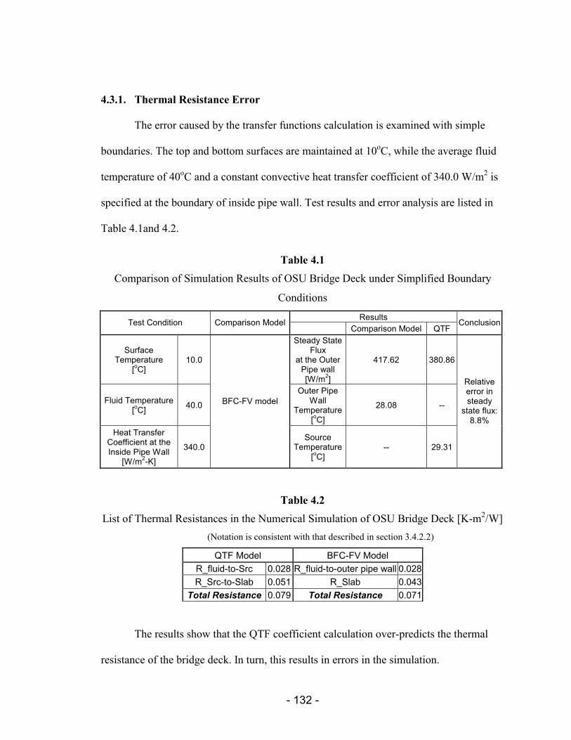
4.3.1. Thermal Resistance Error
The error caused by the transfer functions calculation is examined with simple
boundaries. The top and bottom surfaces are maintained at 10oC, while the average fluid
temperature of 40oC and a constant convective heat transfer coefficient of 340.0 W/m2 is
specified at the boundary of inside pipe wall. Test results and error analysis are listed in
Table 4.1and 4.2.
Table 4.1 Comparison of Simulation Results of OSU Bridge Deck under Simplified Boundary
Conditions
Results Test Condition Comparison Model Comparison Model QTF
Conclusion
Surface Temperature
[oC] 10.0
Steady State Flux
at the Outer Pipe wall [W/m2]
417.62 380.86
Fluid Temperature [oC] 40.0
Outer Pipe Wall
Temperature [oC]
28.08 --
Heat Transfer Coefficient at the Inside Pipe Wall
[W/m2-K]
340.0
BFC-FV model
Source Temperature
[oC] -- 29.31
Relative error in steady
state flux: 8.8%
Table 4.2 List of Thermal Resistances in the Numerical Simulation of OSU Bridge Deck [K-m2/W]
(Notation is consistent with that described in section 3.4.2.2)
QTF Model BFC-FV Model R_fluid-to-Src 0.028 R_fluid-to-outer pipe wall 0.028 R_Src-to-Slab 0.051 R_Slab 0.043
Total Resistance 0.079 Total Resistance 0.071
The results show that the QTF coefficient calculation over-predicts the thermal
resistance of the bridge deck. In turn, this results in errors in the simulation.
- 132 -
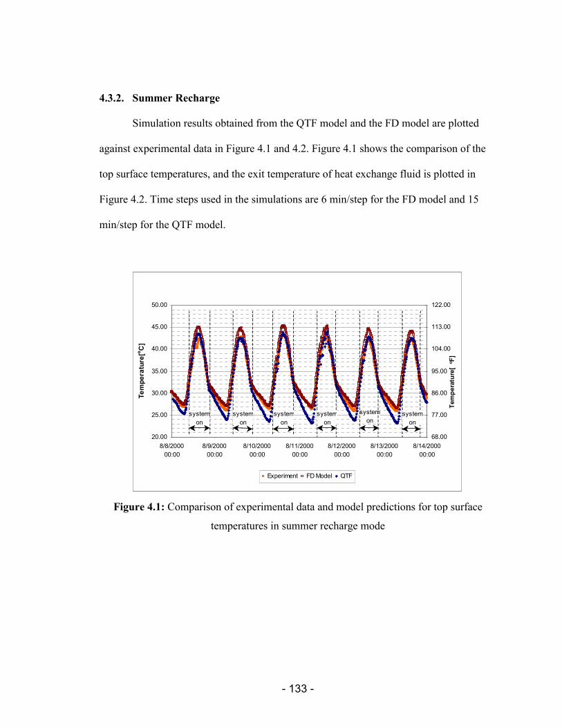
4.3.2. Summer Recharge
Simulation results obtained from the QTF model and the FD model are plotted
against experimental data in Figure 4.1 and 4.2. Figure 4.1 shows the comparison of the
top surface temperatures, and the exit temperature of heat exchange fluid is plotted in
Figure 4.2. Time steps used in the simulations are 6 min/step for the FD model and 15
min/step for the QTF model.
20.00
25.00
30.00
35.00
40.00
45.00
50.00
8/8/200000:00
8/9/200000:00
8/10/200000:00
8/11/200000:00
8/12/200000:00
8/13/200000:00
8/14/200000:00
Tem
pera
ture
[o C]
68.00
77.00
86.00
95.00
104.00
113.00
122.00
Tem
pera
ture
[o F
]
Experiment FD Model QTF
system on
system on
system on
system on
system on
system on
Figure 4.1: Comparison of experimental data and model predictions for top surface
temperatures in summer recharge mode
- 133 -
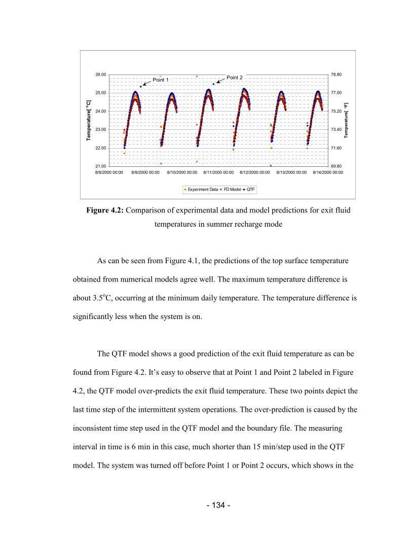
21.00
22.00
23.00
24.00
25.00
26.00
8/8/2000 00:00 8/9/2000 00:00 8/10/2000 00:00 8/11/2000 00:00 8/12/2000 00:00 8/13/2000 00:00 8/14/2000 00:00
Tem
pera
ture
[o C]
69.80
71.60
73.40
75.20
77.00
78.80
Tem
pera
ture
[o F
]
Experiment Data FD Model QTF
Point 2Point 1
Figure 4.2: Comparison of experimental data and model predictions for exit fluid
temperatures in summer recharge mode
As can be seen from Figure 4.1, the predictions of the top surface temperature
obtained from numerical models agree well. The maximum temperature difference is
about 3.5oC, occurring at the minimum daily temperature. The temperature difference is
significantly less when the system is on.
The QTF model shows a good prediction of the exit fluid temperature as can be
found from Figure 4.2. It’s easy to observe that at Point 1 and Point 2 labeled in Figure
4.2, the QTF model over-predicts the exit fluid temperature. These two points depict the
last time step of the intermittent system operations. The over-prediction is caused by the
inconsistent time step used in the QTF model and the boundary file. The measuring
interval in time is 6 min in this case, much shorter than 15 min/step used in the QTF
model. The system was turned off before Point 1 or Point 2 occurs, which shows in the
- 134 -
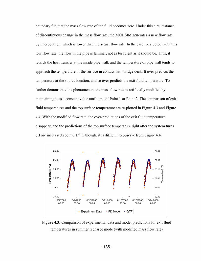
boundary file that the mass flow rate of the fluid becomes zero. Under this circumstance
of discontinuous change in the mass flow rate, the MODSIM generates a new flow rate
by interpolation, which is lower than the actual flow rate. In the case we studied, with this
low flow rate, the flow in the pipe is laminar, not as turbulent as it should be. Thus, it
retards the heat transfer at the inside pipe wall, and the temperature of pipe wall tends to
approach the temperature of the surface in contact with bridge deck. It over-predicts the
temperature at the source location, and so over predicts the exit fluid temperature. To
further demonstrate the phenomenon, the mass flow rate is artificially modified by
maintaining it as a constant value until time of Point 1 or Point 2. The comparison of exit
fluid temperatures and the top surface temperature are re-plotted in Figure 4.3 and Figure
4.4. With the modified flow rate, the over-predictions of the exit fluid temperature
disappear, and the predictions of the top surface temperature right after the system turns
off are increased about 0.13oC, though, it is difficult to observe from Figure 4.4.
21.00
22.00
23.00
24.00
25.00
26.00
8/8/200000:00
8/9/200000:00
8/10/200000:00
8/11/200000:00
8/12/200000:00
8/13/200000:00
8/14/200000:00
Tem
pera
ture
[o C]
69.80
71.60
73.40
75.20
77.00
78.80
Tem
pera
ture
[o F
]
Experiment Data FD Model QTF
Figure 4.3: Comparison of experimental data and model predictions for exit fluid
temperatures in summer recharge mode (with modified mass flow rate)
- 135 -
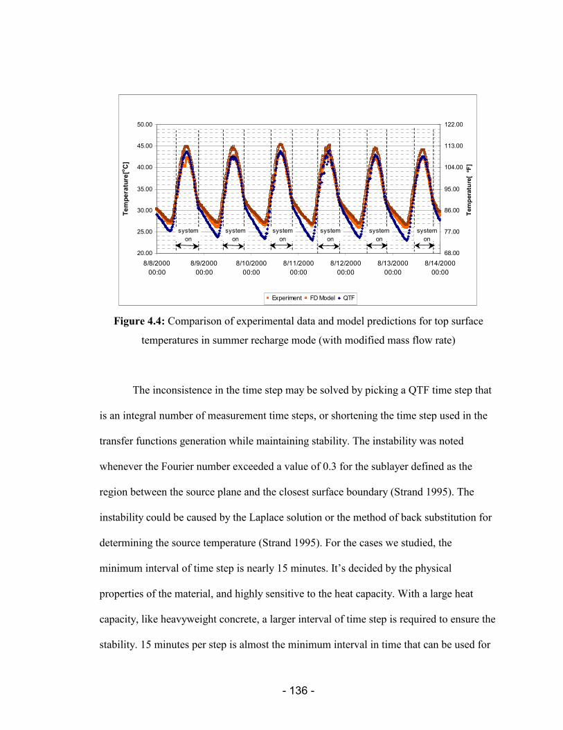
20.00
25.00
30.00
35.00
40.00
45.00
50.00
8/8/200000:00
8/9/200000:00
8/10/200000:00
8/11/200000:00
8/12/200000:00
8/13/200000:00
8/14/200000:00
Tem
pera
ture
[o C]
68.00
77.00
86.00
95.00
104.00
113.00
122.00
Tem
pera
ture
[o F
]
Experiment FD Model QTF
system on
system on
system on
system on
system on
system on
Figure 4.4: Comparison of experimental data and model predictions for top surface
temperatures in summer recharge mode (with modified mass flow rate)
The inconsistence in the time step may be solved by picking a QTF time step that
is an integral number of measurement time steps, or shortening the time step used in the
transfer functions generation while maintaining stability. The instability was noted
whenever the Fourier number exceeded a value of 0.3 for the sublayer defined as the
region between the source plane and the closest surface boundary (Strand 1995). The
instability could be caused by the Laplace solution or the method of back substitution for
determining the source temperature (Strand 1995). For the cases we studied, the
minimum interval of time step is nearly 15 minutes. It’s decided by the physical
properties of the material, and highly sensitive to the heat capacity. With a large heat
capacity, like heavyweight concrete, a larger interval of time step is required to ensure the
stability. 15 minutes per step is almost the minimum interval in time that can be used for
- 136 -
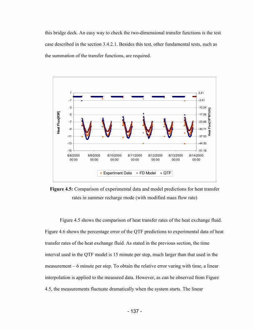
this bridge deck. An easy way to check the two-dimensional transfer functions is the test
case described in the section 3.4.2.1. Besides this test, other fundamental tests, such as
the summation of the transfer functions, are required.
-15
-13
-11
-9
-7
-5
-3
-1
1
8/8/200000:00
8/9/200000:00
8/10/200000:00
8/11/200000:00
8/12/200000:00
8/13/200000:00
8/14/200000:00
Heat
Flu
x[KW
]
-51.18
-44.35
-37.53
-30.71
-23.88
-17.06
-10.24
-3.41
3.41
Hea
t Flu
x[10
3 *B
TU/h
]
Experiment Data FD Model QTF
Figure 4.5: Comparison of experimental data and model predictions for heat transfer
rates in summer recharge mode (with modified mass flow rate)
Figure 4.5 shows the comparison of heat transfer rates of the heat exchange fluid.
Figure 4.6 shows the percentage error of the QTF predictions to experimental data of heat
transfer rates of the heat exchange fluid. As stated in the previous section, the time
interval used in the QTF model is 15 minute per step, much larger than that used in the
measurement – 6 minute per step. To obtain the relative error varing with time, a linear
interpolation is applied to the measured data. However, as can be observed from Figure
4.5, the measurements fluctuate dramatically when the system starts. The linear
- 137 -

interpolation may not be valid at system startup, and it results in larger percentage error at
the beginning of system starts. Most relative error is within the range 10.0%.
Generally, the QTF predictions show a good agreement with the measurements. The
cumulative percentage error is around 2.4% for the period shown in the figures.
�
-100.00%
-80.00%
-60.00%
-40.00%
-20.00%
0.00%
20.00%
40.00%
60.00%
80.00%
100.00%
8/8/200000:00
8/9/200000:00
8/10/200000:00
8/11/200000:00
8/12/200000:00
8/13/200000:00
8/14/200000:00
Perc
enta
ge E
rror
in H
eat F
lux
Figure 4.6: Percentage error of the QTF predictions to experimental data on heat transfer
rates in summer recharge mode (with modified mass flow rate)
4.3.3. Winter Heating
Weather data for a winter heating event are plotted in Figure 4.7. The snow
precipitation rate is given as equivalent mm of water. As accurate precipitation data in
freezing conditions is not available from the automated experimental bridge site, the
snow precipitation plotted is the average over time (only the total precipitation for the
snow event is available). Simulations start from 12/24/2001 00:00.
- 138 -
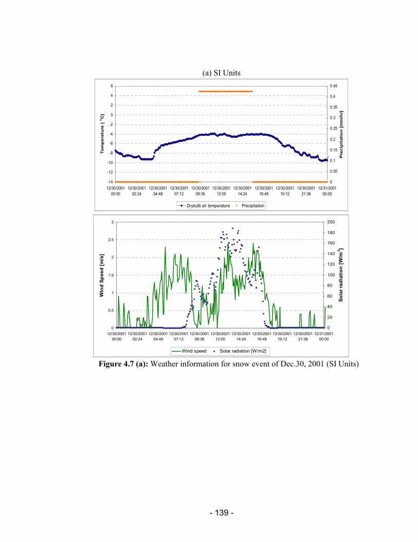
(a) SI Units
-14
-12
-10
-8
-6
-4
-2
0
2
4
6
12/30/200100:00
12/30/200102:24
12/30/200104:48
12/30/200107:12
12/30/200109:36
12/30/200112:00
12/30/200114:24
12/30/200116:48
12/30/200119:12
12/30/200121:36
12/31/200100:00
Tem
per
atu
re [
oC
]
0
0.05
0.1
0.15
0.2
0.25
0.3
0.35
0.4
0.45
Pre
cip
itat
ion
[m
m/h
r]
Drybulb air temperature Precipitation
0
0.5
1
1.5
2
2.5
3
12/30/200100:00
12/30/200102:24
12/30/200104:48
12/30/200107:12
12/30/200109:36
12/30/200112:00
12/30/200114:24
12/30/200116:48
12/30/200119:12
12/30/200121:36
12/31/200100:00
Win
d Sp
eed
[m/s
]
0
20
40
60
80
100
120
140
160
180
200
Sola
r rad
iatio
n [W
/m2 ]
Wind speed Solar radiation [W/m2]
Figure 4.7 (a): Weather information for snow event of Dec.30, 2001 (SI Units)
- 139 -
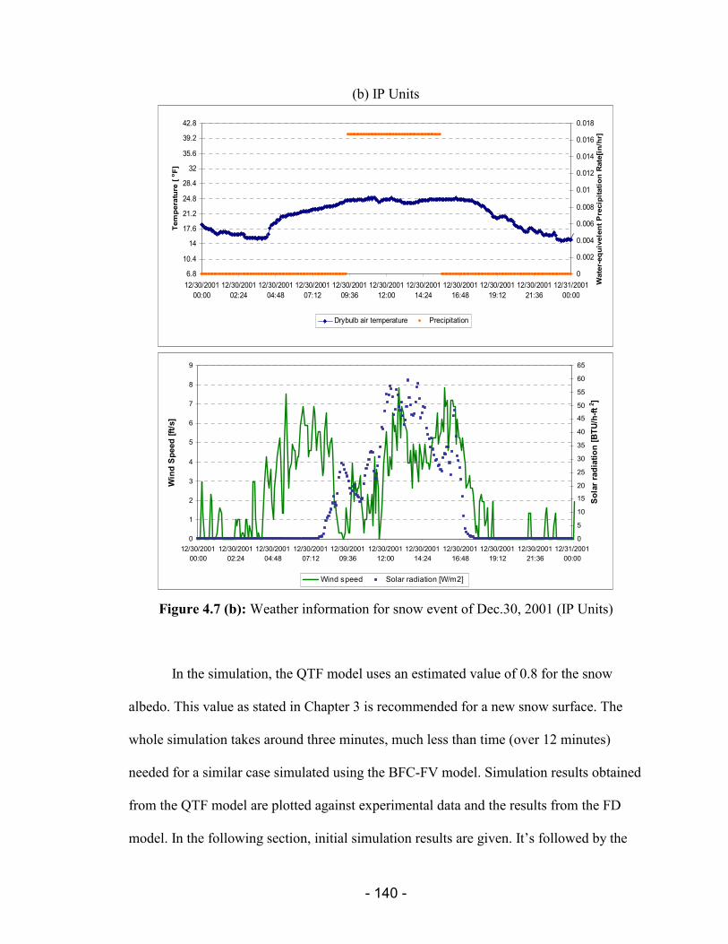
(b) IP Units
6.8
10.4
14
17.6
21.2
24.8
28.4
32
35.6
39.2
42.8
12/30/200100:00
12/30/200102:24
12/30/200104:48
12/30/200107:12
12/30/200109:36
12/30/200112:00
12/30/200114:24
12/30/200116:48
12/30/200119:12
12/30/200121:36
12/31/200100:00
Tem
pera
ture
[oF]
0
0.002
0.004
0.006
0.008
0.01
0.012
0.014
0.016
0.018
Wat
er-e
quiv
elen
t Pre
cipi
tatio
n R
ate[
in/h
r]
Drybulb air temperature Precipitation
0
1
2
3
4
5
6
7
8
9
12/30/200100:00
12/30/200102:24
12/30/200104:48
12/30/200107:12
12/30/200109:36
12/30/200112:00
12/30/200114:24
12/30/200116:48
12/30/200119:12
12/30/200121:36
12/31/200100:00
Win
d Sp
eed
[ft/s
]
0
5
10
15
20
25
30
35
40
45
50
55
60
65
Sola
r rad
iatio
n [B
TU/h
-ft2 ]
Wind speed Solar radiation [W/m2]
Figure 4.7 (b): Weather information for snow event of Dec.30, 2001 (IP Units)
In the simulation, the QTF model uses an estimated value of 0.8 for the snow
albedo. This value as stated in Chapter 3 is recommended for a new snow surface. The
whole simulation takes around three minutes, much less than time (over 12 minutes)
needed for a similar case simulated using the BFC-FV model. Simulation results obtained
from the QTF model are plotted against experimental data and the results from the FD
model. In the following section, initial simulation results are given. It’s followed by the
- 140 -
discussion of possible corrections and the presentation of results after making individual
modification. Last come the final results with recommended corrections. Time interval is
5 min/step for the measurement and 15 min/step for the QTF model.
Initial simulation results
Figure 4.8 shows the initial simulation results. The discrepancy in temperature
between the experimental measurements and the numerical predictions are obvious.
However, at the beginning of storm and several hours after storm, the results obtained
from the QTF model agree with those from the FD model. One possible cause of the
initial discrepancy is the inaccuracy of weather data shared by two numerical models, like
sky temperature. Inaccuracy in calculating the convection and radiation occurring at the
surfaces is probably another cause. Two numerical models use different formulas for the
convection and radiation calculation on the slab surfaces. There have been many different
methods published for calculating the convective coefficient, with much disparity among
them. Identifying the best correlation for the bridge deck heating case may require more
future work.
After the storm starts, one cause of the discrepancy in temperature between the
numerical solutions and the experimental measurement is the assumed constant snow
precipitation (rather than actual time-varying snow precipitation). Another possible cause
is that the experimental temperature measurements are made slightly below the slab
surface, and are expected to be higher than the top surface temperature in the winter.
- 141 -
However, there is a big difference between the numerical solutions after the
surface temperature reaches the freezing point. The restriction in the QTF model, that the
surface temperature would be maintained at the freezing point when snow, ice, or snow
slush was melting on the surface, makes the surface temperature keep as constant (0oC)
for a period. After the surface is clean of snow and slush, the top surface temperature
obtained for the QTF model creeps up. While in the FD model, without the restriction to
maintain the surface at the freezing when the slab was covered by snow or ice, the
surface temperature creeps up continuously. The surface temperatures fluctuate with the
intermittent system operations as shown in Figure 4.8 (a).
The numerical solution on the exit fluid temperature obtained for the QTF model
agrees well with the experimental measurements as can be observed from Figure 4.8 (b).
- 142 -
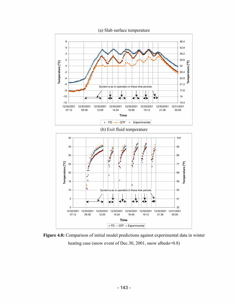
(a) Slab surface temperature
-12
-10
-8
-6
-4
-2
0
2
4
6
8
12/30/200107:12
12/30/200109:36
12/30/200112:00
12/30/200114:24
12/30/200116:48
12/30/200119:12
12/30/200121:36
12/31/200100:00
Time
Tem
pera
ture
[o C]
10.4
14
17.6
21.2
24.8
28.4
32
35.6
39.2
42.8
46.4
Tem
pera
ture
[o F]
FD QTF Experimental
System w as in operation in these time periods.
(b) Exit fluid temperature
0
5
10
15
20
25
30
35
40
12/30/200107:12
12/30/200109:36
12/30/200112:00
12/30/200114:24
12/30/200116:48
12/30/200119:12
12/30/200121:36
12/31/200100:00
Time
Tem
pera
ture
[o C]
32
41
50
59
68
77
86
95
104
Tem
pera
ture
[o F]
FD QTF Experimental
System w as in operation in these time periods.
Figure 4.8: Comparison of initial model predictions against experimental data in winter
heating case (snow event of Dec.30, 2001, snow albedo=0.8)
- 143 -
Possible corrections and simulation results
Several corrections are considered in the following section. These include the
correction of sky temperature, the estimation of the value of snow albedo, and the thermal
properties of saturated slab surface.
As described in Chapter 3, sky temperatures are calculated based on other
available weather data, such as dry-bulb air temperature, humidity ratio, cloud cover
factor, etc. However, the cloud cover fraction is not easy to measure accurately. The
cloud cover data used in the validation is obtained by combining cloud cover data from
the National Virtual Data system with the data from the Oklahoma Mesonet (Liu et al.
2002). Inaccuracies in estimating the sky temperature lead to deviations in the surface
temperature calculation especially during nights when long-wave radiation has a greater
proportion in the heat transfer rate occurring at the surfaces. The modified sky
temperatures used in the following simulations are calculated by the Brown sky
temperature model with the assumption that from 24 hours before the snow event till the
end of the storm, the cloud fraction is assumed as 1.0.
Snow albedo (snow reflectance) determines the proportion of solar radiation
absorbed by the snow/slush. The estimated value of snow albedo used in this case is 0.8
assuming a new snow surface covering the slab during precipitation. This approximation
is not necessarily accurate at the end of the snow-melting process, when the slab surface
is warm enough to melt the precipitation as soon as it falls on the slab, and the surface is
covered by the slush. Another lower estimation of snow albedo, 0.38, is used to illustrate
- 144 -
the effect of snow albedo estimation. This lower estimation of snow albedo makes the
snow surface have the same absorptance as slab surface. Besides two estimations, a time
varying snow albedo calculated by the QTF model is used for further analysis.
The following section also describes the effect of the change in the physical
properties of the slab when it’s saturated. During the snow-melting process, the slab
surface may be wet and saturated. The conductivity and specific heat of the concrete in
saturated condition are different from values of dry concrete. For instance, for the
material currently used, the specific heat varies between 898 and1037 J/kg-K when it’s at
oven-dry, normally dry, and saturated conditions; the change is over 10%.
The correction of physical properties is achieved by switching transfer functions
generated by different inputs properties in the simulation. (This is a rough approximation;
it doesn’t correctly account for the history). An estimation of time required for the
surface to reach saturated is used. When the surface is wet for 45 consecutive minutes,
the slab surface is considered saturated, and the set of transfer functions generated by
using the saturated concrete properties are used in the simulation. Once the slab surface is
dry, the set of transfer functions generated by using the concrete properties under the dry
condition are restored.
- 145 -
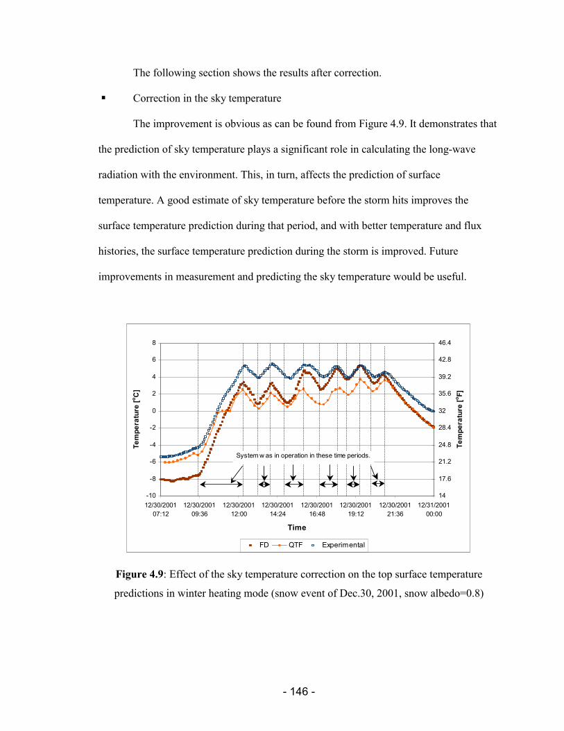
The following section shows the results after correction.
�� Correction in the sky temperature
The improvement is obvious as can be found from Figure 4.9. It demonstrates that
the prediction of sky temperature plays a significant role in calculating the long-wave
radiation with the environment. This, in turn, affects the prediction of surface
temperature. A good estimate of sky temperature before the storm hits improves the
surface temperature prediction during that period, and with better temperature and flux
histories, the surface temperature prediction during the storm is improved. Future
improvements in measurement and predicting the sky temperature would be useful.
-10
-8
-6
-4
-2
0
2
4
6
8
12/30/200107:12
12/30/200109:36
12/30/200112:00
12/30/200114:24
12/30/200116:48
12/30/200119:12
12/30/200121:36
12/31/200100:00
Time
Tem
pera
ture
[o C]
14
17.6
21.2
24.8
28.4
32
35.6
39.2
42.8
46.4
Tem
pera
ture
[o F]
FD QTF Experimental
System w as in operation in these time periods.
Figure 4.9: Effect of the sky temperature correction on the top surface temperature
predictions in winter heating mode (snow event of Dec.30, 2001, snow albedo=0.8)
- 146 -
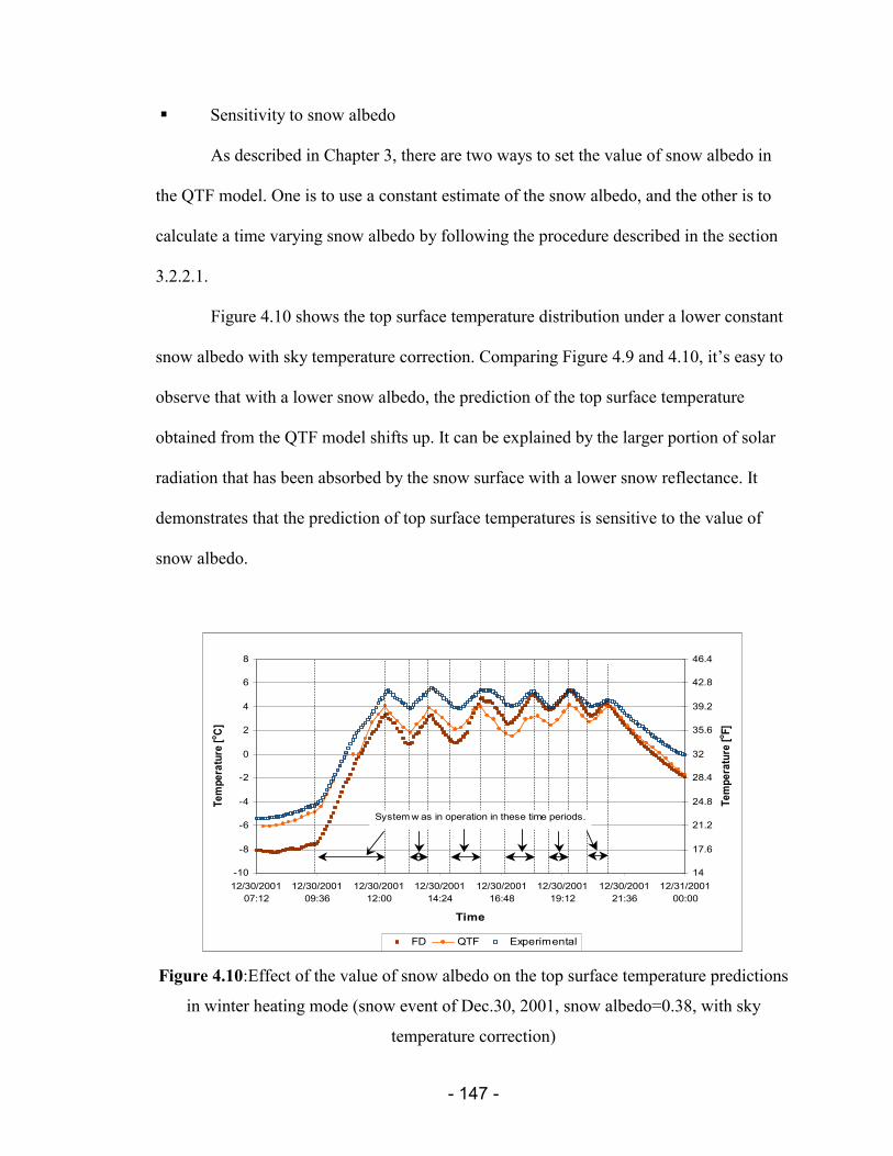
�� Sensitivity to snow albedo
As described in Chapter 3, there are two ways to set the value of snow albedo in
the QTF model. One is to use a constant estimate of the snow albedo, and the other is to
calculate a time varying snow albedo by following the procedure described in the section
3.2.2.1.
Figure 4.10 shows the top surface temperature distribution under a lower constant
snow albedo with sky temperature correction. Comparing Figure 4.9 and 4.10, it’s easy to
observe that with a lower snow albedo, the prediction of the top surface temperature
obtained from the QTF model shifts up. It can be explained by the larger portion of solar
radiation that has been absorbed by the snow surface with a lower snow reflectance. It
demonstrates that the prediction of top surface temperatures is sensitive to the value of
snow albedo.
-10
-8
-6
-4
-2
0
2
4
6
8
12/30/200107:12
12/30/200109:36
12/30/200112:00
12/30/200114:24
12/30/200116:48
12/30/200119:12
12/30/200121:36
12/31/200100:00
Time
Tem
pera
ture
[o C]
14
17.6
21.2
24.8
28.4
32
35.6
39.2
42.8
46.4
Tem
pera
ture
[o F]
FD QTF Experimental
System w as in operation in these time periods.
Figure 4.10:Effect of the value of snow albedo on the top surface temperature predictions
in winter heating mode (snow event of Dec.30, 2001, snow albedo=0.38, with sky
temperature correction)
- 147 -
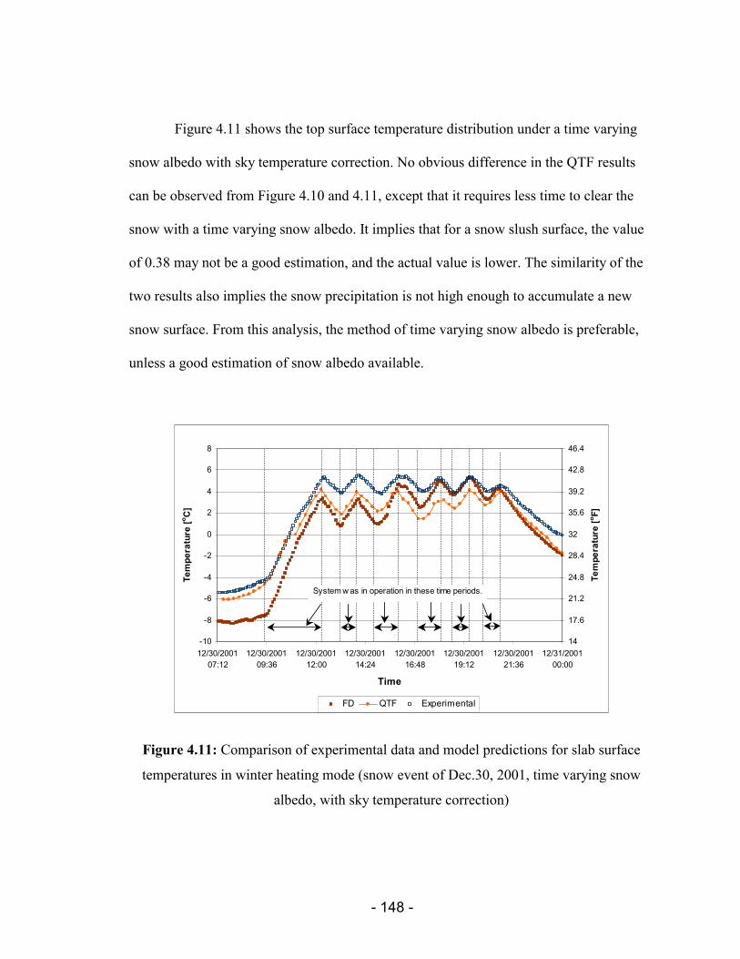
Figure 4.11 shows the top surface temperature distribution under a time varying
snow albedo with sky temperature correction. No obvious difference in the QTF results
can be observed from Figure 4.10 and 4.11, except that it requires less time to clear the
snow with a time varying snow albedo. It implies that for a snow slush surface, the value
of 0.38 may not be a good estimation, and the actual value is lower. The similarity of the
two results also implies the snow precipitation is not high enough to accumulate a new
snow surface. From this analysis, the method of time varying snow albedo is preferable,
unless a good estimation of snow albedo available.
-10
-8
-6
-4
-2
0
2
4
6
8
12/30/200107:12
12/30/200109:36
12/30/200112:00
12/30/200114:24
12/30/200116:48
12/30/200119:12
12/30/200121:36
12/31/200100:00
Time
Tem
pera
ture
[o C]
14
17.6
21.2
24.8
28.4
32
35.6
39.2
42.8
46.4
Tem
pera
ture
[o F]
FD QTF Experimental
System w as in operation in these time periods.
Figure 4.11: Comparison of experimental data and model predictions for slab surface
temperatures in winter heating mode (snow event of Dec.30, 2001, time varying snow
albedo, with sky temperature correction)
- 148 -
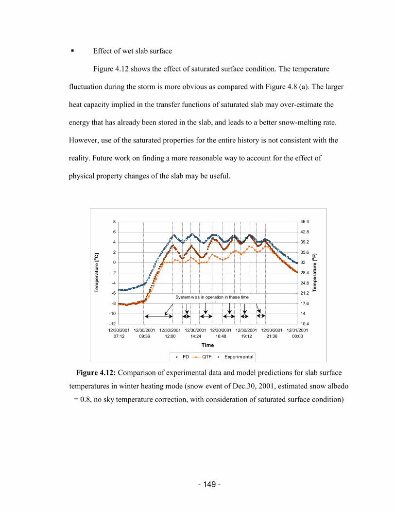
�� Effect of wet slab surface
Figure 4.12 shows the effect of saturated surface condition. The temperature
fluctuation during the storm is more obvious as compared with Figure 4.8 (a). The larger
heat capacity implied in the transfer functions of saturated slab may over-estimate the
energy that has already been stored in the slab, and leads to a better snow-melting rate.
However, use of the saturated properties for the entire history is not consistent with the
reality. Future work on finding a more reasonable way to account for the effect of
physical property changes of the slab may be useful.
-12
-10
-8
-6
-4
-2
0
2
4
6
8
12/30/200107:12
12/30/200109:36
12/30/200112:00
12/30/200114:24
12/30/200116:48
12/30/200119:12
12/30/200121:36
12/31/200100:00
Time
Tem
pera
ture
[o C]
10.4
14
17.6
21.2
24.8
28.4
32
35.6
39.2
42.8
46.4
Tem
pera
ture
[o F]
FD QTF Experimental
System w as in operation in these time periods
Figure 4.12: Comparison of experimental data and model predictions for slab surface
temperatures in winter heating mode (snow event of Dec.30, 2001, estimated snow albedo
= 0.8, no sky temperature correction, with consideration of saturated surface condition)
- 149 -
Final results
Figure 4.13 serves as the final simulation results with the consideration of the
correction in the sky temperature and a time varying snow albedo. The improvement is
obvious as compared with Figure 4.8.
The surface temperature obtained from the QTF model agrees with the
measurements when there is no precipitation. Also, a good agreement can be observed
before the surface temperature reaches the freezing point after the storm starts. The
discrepancy during snow precipitation is obvious, and as stated in the previous section, it
may be caused by the make-up snow precipitation data and the location of thermocouples.
After the storm, the temperature comes to a new low at around 17:00. It can be explained
by the fact that the unit cloud cover assumption is ended with the storm, and a larger
radiation loss occurs at the surface. Without the correction of the sky temperature, the
predictions from the QTF model tend to agree with those from the FD model.
The exit fluid temperature predictions agree well with experimental data, and it
implies a good agreement in the heat transfer rate in the heat exchange fluid side. As can
be observed from Figure 4.13 (b), the start/stop times of the bridge heating don’t quite
match the experimental data. This is caused by the large time step used in the QTF model.
- 150 -
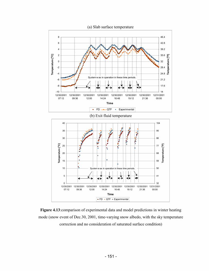
(a) Slab surface temperature
-10
-8
-6
-4
-2
0
2
4
6
8
12/30/200107:12
12/30/200109:36
12/30/200112:00
12/30/200114:24
12/30/200116:48
12/30/200119:12
12/30/200121:36
12/31/200100:00
Time
Tem
pera
ture
[o C]
14
17.6
21.2
24.8
28.4
32
35.6
39.2
42.8
46.4
Tem
pera
ture
[o F]
FD QTF Experimental
System w as in operation in these time periods.
(b) Exit fluid temperature
0
5
10
15
20
25
30
35
40
12/30/200107:12
12/30/200109:36
12/30/200112:00
12/30/200114:24
12/30/200116:48
12/30/200119:12
12/30/200121:36
12/31/200100:00
Time
Tem
pera
ture
[o C]
32
41
50
59
68
77
86
95
104
Tem
pera
ture
[o F]
FD QTF Experimental
System w as in operation in these time periods.
Figure 4.13:comparison of experimental data and model predictions in winter heating
mode (snow event of Dec.30, 2001, time-varying snow albedo, with the sky temperature
correction and no consideration of saturated surface condition)
- 151 -
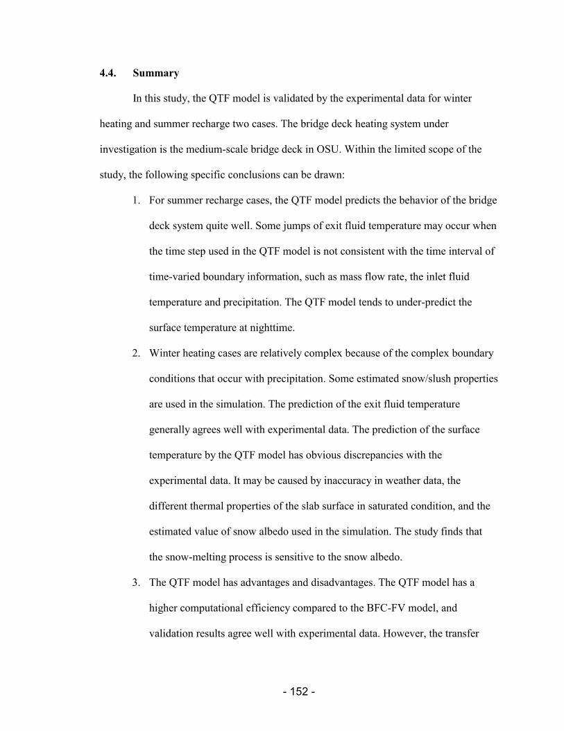
4.4. Summary
In this study, the QTF model is validated by the experimental data for winter
heating and summer recharge two cases. The bridge deck heating system under
investigation is the medium-scale bridge deck in OSU. Within the limited scope of the
study, the following specific conclusions can be drawn:
1. For summer recharge cases, the QTF model predicts the behavior of the bridge
deck system quite well. Some jumps of exit fluid temperature may occur when
the time step used in the QTF model is not consistent with the time interval of
time-varied boundary information, such as mass flow rate, the inlet fluid
temperature and precipitation. The QTF model tends to under-predict the
surface temperature at nighttime.
2. Winter heating cases are relatively complex because of the complex boundary
conditions that occur with precipitation. Some estimated snow/slush properties
are used in the simulation. The prediction of the exit fluid temperature
generally agrees well with experimental data. The prediction of the surface
temperature by the QTF model has obvious discrepancies with the
experimental data. It may be caused by inaccuracy in weather data, the
different thermal properties of the slab surface in saturated condition, and the
estimated value of snow albedo used in the simulation. The study finds that
the snow-melting process is sensitive to the snow albedo.
3. The QTF model has advantages and disadvantages. The QTF model has a
higher computational efficiency compared to the BFC-FV model, and
validation results agree well with experimental data. However, the transfer
- 152 -
functions are generated by another program in advance. The limitation is that,
for the QTF model, the time step must be fixed in the simulation to be the
same as that used in the transfer functions generation. The variable time step
is not allowed in the application of the QTF model. Limited by the transfer
functions, the QTF model can’t provide detailed two-dimensional temperature
and flux distributions. Only average values are available.
This work opens a number of areas for further study. The validation in this work
is not sufficient to draw a general conclusion. Further research is suggested in the
following areas:
�� Additional work in sky temperature estimation would be useful.
�� Additional experimental work in snow-melting cases is required. These may
include the measurement of snow albedo, the sky temperature, detailed record
of surface conditions (i.e. dry, wet, snow/slush), and thermal properties of
slab surface in saturation.
�� Additional validation of the QTF model, using experimental data and a wider
range of transient weather condition, would be useful.
�� The inconsistence in the time step may be solved by picking a QTF time step
that is an integral number of measurement time steps, or shortening the time
step used in the transfer functions generation while maintaining stability.
�� Validation of the QTF model for other related applications, such as modeling
the performance snow melting systems in pavement, would be useful.
- 153 -
5. Conclusions and Recommendations
5.1. Conclusions
As the size and the number of applications of hydronic and electric-cable snow-
melting systems increase, economic design and optimization become increasingly
important. Considerable savings in cost and effort could be realized if the performance of
such systems could be easily simulated and analyzed. The system modeling and
simulation approach is a powerful tool to study and analyze the system performance of
several possible designs. Various system configurations, component sizes, and different
control strategies could be studied using the system simulation approach to arrive at cost
efficient design solutions. Both short and long-term system performance could be easily
simulated using validated numerical models.
This study uses the simulation approach to analyze the applications of hydronic
and electric-cable snow-melting systems. The challenges associated with the analysis
originate from the transient nature of weather and the intermittent operation of systems.
The objectives of this study were threefold: (1) to examine the effects of different
parameters on transient system performance, (2) to develop a design and simulation tool
for modeling the transient performance of a hydronic and electric-cable snow-melting
systems by time series method (QTFs), and (3) to validate the transient QTF model by
experimental data.
- 154 -
Chapter 2 of this thesis has presented a parametric study of hydronic and electric-
cable snow-melting systems. The effects of two phenomena on the transient snow-
melting system behavior have been investigated. One is back and edge losses, and the
other is transient design conditions and operation of the snow-melting system. The
studied parameters include pipe spacing, pipe depth, pipe diameter, insulation level, soil
conductivity, location, and storm. The transient load requirements are not closely
correlated to the steady-state loads. More than any other factor, the transient behavior is
most sensitive to the storm itself, and then to pipe spacing. As the tubes are placed
deeper, the effect of spacing is less important. The heat flux requirements at the source
location are almost insensitive to the soil conductivity and the insulation level. Insulation
is useful for reducing back losses.
Chapter 3 of this thesis has described the development and validation of a model
(the QTF model) for simulating the transient performance hydronic and electric-cable
snow-melting systems by time series method (QTFs). The QTF model has been coupled
to HVACSim+ environment. The simulation results are compared with the analytical
solution, and the results from other software. It’s found that the transfer functions
calculator has inaccuracies in generating the transfer functions, which leads to 8%~15%
error in the steady state flux in the simulation.
Chapter 4 discusses the validation of the QTF model developed in Chapter 3 by
experimental data obtained from a medium-scale bridge deck located at OSU. The
simulations have been done under real transient weather conditions with operation and
- 155 -
construction parameters from a working system. Within cases that have been studied, the
QTF model gives good predictions on the exit fluid temperature with maximum error of
around 0.3oC (0.54oF). For the surface temperature, the simulation results agree with the
experimental data, except for the situation of snow precipitations. The maximum error in
the case of summer recharge is 3.5oC (6.3oF), occurring when the system is off. When
system is on, the error is significant less, and the QTF model gives accurate predictions
on the surface temperature. The cumulative error of the energy recharged to the ground is
around 2.4% compared to the experimental data. For winter heating case, the surface
temperature predictions agree with the experimental measurements after the correction of
the sky temperature is applied. However, there is a big difference (around 2oC (3.6oF)) in
surface temperature predictions during the snow precipitation. This difference implies a
different surface condition on the slab. The assumed constant snow precipitation rate is
one cause of this difference. Another possible cause is that the experimental temperature
measurements are made slightly below the slab surface, and are expected to be higher
than the slab surface temperature in the winter heating cases. Results show that the snow-
melting process is sensitive to the snow albedo estimate. More experimental work is
needed for validation of surface condition in snow-melting cases.
5.2. Recommendations
Though the work presented in this thesis is a step towards a better understanding
of transient performance of performance hydronic and electric-cable snow-melting
systems, its scope is limited. Further research is suggested in the following areas:
�� Additional experimental work on snow-melting cases would be helpful.
- 156 -

�� Additional work on sky temperature estimation with consideration of cloud
cover data would be helpful.
�� Additional validation of the QTF model, using experimental data and a wider
range of transient weather condition, would be useful.
�� Validation of the QTF model to other applications, such as modeling the
performance snow melting systems in pavement, would be useful.
- 157 -
REFERENCES
ASHRAE Handbook — Fundamentals, 1993. Atlanta, GA: American Society of Heating Refrigerating and Air-conditioning Engineers Inc.
ASHRAE Handbook — Applications, 1999. Atlanta, GA: American Society of Heating Refrigerating and Air-conditioning Engineers Inc.
ASHRAE Toolkit for Building Load Calculations —Manual, 2001. Atlanta, GA: American Society of Heating Refrigerating and Air-conditioning Engineers Inc.
Brown, D. 1996. Development of an improved meteorological preprocessor and applied dispersion model. Ph.D. dissertation, University of Illinois at Urbana-Champaign, Department of Mechanical and Industrial Engineering
Chapman, W.P., 1952. Design of Snow Melting Systems. Heating and Ventilating, Vol. 49(4), pp: 96-102.
Chapman, W.P., 1952. Design of Snow Melting Systems. Heating and Ventilating, Vol. 49(11), pp: 88-95.
Chapman, W.P. and S. Katunich, 1956. Heat Requirements of Snow Melting Systems. Heating, Piping & Air Conditioning, Vol. 28(2), pp: 149-153.
Chapman, W.P., 1957. Calculating the Heat Requirements of Snow Melting Systems. Air Conditioning, Heating and Ventilating, Vol. 54(8), pp: 81-96.
Chiasson, A. 2000. Advances in Modeling of Ground-Source Heat Pump Systems. M.S. Thesis. Oklahoma State University. Stillwater, OK. (Also available at http://www.hvac.okstate.edu/pdfs/chiasson_thesis.pdf).
Clark, D.R., 1985. HVACSim+ Building System and Equipment Simulation Program – Reference Manual. National Bureau of Standards. NBSIR 84-2996.
Gnielinski, V. 1976. New equations for heat and mass transfer in turbulent flow pipes and ducts. International Chemical Engineering, Vol. 16, pp: 359-367.
Gordon, W.J. and Hall, C.A. 1973. Construction of curvilinear coordinate systems and applications to mesh generation. International Journal for Numerical Methods in Engineering, Vol. 7(4), pp. 461-477.
Incropera, F.P., and D.P. Dewitt. 1996. Introduction to Heat Transfer, pp: 332-334. New York: Wiley & Sons
Kilkis I. B. 1994a. Design of embedded snow-melting systems. Part 1, Heat requirements - an overall assessment and recommendations. ASHRAE Transactions, Vol. 100, Part 1, pp: 423-433.
Kilkis I. B. 1994b. Design of embedded snow-melting systems. Part 2, Heat transfer in the slab - a simplified model. ASHRAE Transactions, Vol. 100, Part 1, pp: 434-441.
Kondo, J., and T. Yamazaki 1990. A Prediction Model for Snowmelt, Snow Surface Temperature and Freezing Depth Using a Heat Balance Method. Journal of Applied Meteorology 29:375-384.
- 158 -
Kusuda, T., P.R. Achenbach 1965, Earth Temperature and Thermal Diffusivities at Selected Stations in the United States. ASHRAE Transactions, Vol. 71, pp: 61-76.
Leal, M.R.L.V., P.L. Miller. 1972. An Analysis of the Transient Temperature Distribution in Pavement Heating Installations. ASHRAE Transactions, Vol. 78, Part 2, pp: 61-66.
Liu, X, S.J. Rees, J.D. Spitler. 2002. Simulation of a Geothermal Bridge Deck Anti-icing System and Experimental Validation. Submitted to the TRB 82nd Annual Meeting.
Luikov, A.V. 1968. Analytical heat diffusion theory. New York: Academic Press.
Potter, W.G. 1967. Electric snow melting systems. ASHRAE Journal 9(10), pp: 35-44.
Ramamoorthy, M. 2001. Applications of hybrid ground source heat pump systems to buildings and bridge decks. M.S. Thesis. Oklahoma State University, Stillwater, OK. (Also available at http://www.hvac.okstate.edu/pdfs/Ramamoorthy_Thesis.pdf ).
Ramsey, J.W., H.D. Chiang, R.J. Goldstein, 1982. A study of the incoming long-wave atmospheric radiation from a clear sky. J. Appl. Meterol. 21, pp: 566-578.
Ramsey, J.W., M.J. Hewett, T.H. Kuen, S.D. Petersen. 1999, Updated Design Guidelines for Snow Melting Systems. ASHRAE Transactions. 105(1), pp:1055-1065.
Ramsey, J.W., M.J. Hewett, T.H. Kuen, S.D. Petersen. T.J. Spielman, A. Briefer, (1999), Development of Snow Melting Load Design Algorithms and Data for Locations Around the world (ASHRAE 926-RP), Final Report. Atlanta: American Society of Heating Refrigerating and Air conditioning Engineers Inc.
Rees, S.J., J.D. Spitler, X. Xiao. 2002. Transient analysis of snow-melting system performance. ASHRAE Transactions, 108(2). In press.
Schnurr, N.M., D.B. Rogers. 1970. Transient Analysis of Snow Melting Systems. ASHRAE Transactions, Vol. 77, Part 2, pp: 159-166.
Schnurr, N.M., M.W. Falk. 1973. Heat Transfer Design Data for Optimization of Snow Melting Systems. ASHRAE Transactions, Vol. 76, Part 2, pp: 257-263.
Sparrow, E.M., J.W. Ramsey, E.A.Mass, 1979. Effect of finite width on heat transfer and fluid flow about an inclined rectangular plate. Journal of Heat Transfer Vol.101, n 2, pp: 199-204.
Spitler, J.D., S.J. Rees, D. Xiao. 2002. Development of an Analytical Verification Test Suite for Whole Building Energy Simulation Programs - Building Fabric (RP-1052), Final Report, Atlanta, GA: American Society of Heating Refrigerating and Air-conditioning Engineers Inc.
Spitler, J.D., S.J. Rees, X. Xiao, M. Chulliparambil. 2001. Development Of A Two-Dimensional Transient Model Of Snow-Melting Systems, And Use Of The Model For Analysis Of Design Alternatives (RP-1090), Final Report, Atlanta, GA: American Society of Heating Refrigerating and Air-conditioning Engineers Inc.
Spitler, J.D., (2001), Progress Report, Aug. 2001. Oklahoma State University Geothermal Smart Bridge Research Project.
- 159 -
Stone, H.L. 1968. Iterative Solution of Implicit Approximations of Multidimensional Partial Differential Equations. SIAM Journal of Numerical Analysis. Vol.5, No.3, pp: 530-558.
Strand, R.K. 1995, Heat source transfer functions and their application to low temperature radiant heating systems, Ph.D. dissertation, University of Illinois at Urbana-Champaign, Department of Mechanical and Industrial Engineering.
Strand, R.K., Pedersen, Curtis O. 1997, Implementation of a radiant heating and cooling model into an integrated building energy analysis program, ASHRAE Transactions, v 103, n 1, 1997, pp 949-958.
Tarboton, D. G. and C. H. Luce, 1996. Utah Energy Balance Snow Accumulation and Melt Model (UEB). Utah Water Research Laboratory and USDA Forest Service Intermountain Research Station.
Thomoson, J.F., Waris, Z.U.A., and Mastin, C.W. 1985, Numerical Grid Generation-Foundations and Applications. Elsevier Science Publishing Co., Inc.
Vansant, J.H. 1983. Conduction heat transfer solutions. Lawrence Livemore National Laboratory, University of California. UCRL-52863 Rev.1.
Walton, G.N. 1981. Passive solar extension of the Building Loads Analysis and System Thermodynamics (BLAST) program. Technical Report, United Stated Army Construction Engineering research Laboratory, Champaign, IL.
Walton, G.N. 1983. Thermal analysis research program reference manual. National Bureau of Standards. NBSSIR 83-2655.
Williamson, P.J. 1967. The estimation of heat outputs for road heating installations. Transport Road Research Laboratory (UK): Report LR77. pp: 63.
- 160 -

APPENDIXES
- 161 -

Appendix A: Description of the QTF model in TYPAR.DAT
548 'QTF MODEL'
0 0 11 2 22 ! Numbers of SAVED, Diff. Eq., XIN, OUT, PA
3 'Tamb[C]'
3 'Tsky [C]'
3 'Inlet Fluid Temperature [C]'
4 'Humidity Ratio [kg Water/kg Dry Air]'
4 'Wind Speed [m/s]'
4 'Wind Direction [Degree]'
4 ' Solar Gain [W/m2] '
4 'Solar Zenith Angel [Degree]'
4 'Snow Precip(Precipitation) [mm/h]'
4 'Rain Precip(Precipitation) [mm/h]'
4 'Inlet Mass Flow Rate [kg/s]'
#
3 'Exit Fluid Temperature' '[C]'
6 'PipeFlux' '[W/Circuit]'
#
4 'Latitude'
4 'Longitude'
4 'TimeZone'
4 'Surface Facing'
4 'Surface Tilt'
4 'Ground Reflect'
4 'Surface Emittance'
4 'Surface Absorptance'
4 'Number of Circuit'
4 'null(for future use)'
4 'Fluid Type' '1 for water, 2 for Propylene Glycol'
4 '% WT. OF Propylene Glycol in solution used)' '%'
4 'Pipe Length per Circuit' '[m]'
4 'Pipe Spacing' '[m]'
4 'Pipe Outside Diameter' '[m]'
4 'Bridge Width' '[m]'
4 'Bridge Length' '[m]'
4 'Thermal Conductivity of Pipe' ['W/m-K]'
4 'Thickness of Pipe Wall' '[m]'
4 'Insulation at the Bottom 1/yes, 0/no'
4 'Source Type,1 for temp. control, 2 for flux control'
4 'Source Flux [W/m2]'
- 162 -
VITA
Xia Xiao
Candidate for the Degree of
Master of Science
Thesis: MODELING OF HYDRONIC AND ELECTRIC-CABLE SNOW-
MELTING SYSTEMS FOR PAVEMENTS AND BRIDGE DECKS
Major Field: Mechanical and Aerospace Engineering Biographical:
Personal Data: Born in Nanchang, P.R.China, Jan. 31, 1978, the daughter of Yuli
Jia and Zhizhen Xiao. Education: Received Bachelor of Science Degree in Thermal Engineering from
Tsinghua University, P. R. China, in May, 2000; Completed the requirements for Master of Science degree at Oklahoma State University in December 2002.
Experience: Employed by the Oklahoma State University from August 2000 to
August 2002 as research assistant. Professional Membership: ASHRAE