Embed Size (px)
Citation preview

Risk Modeling of Multi‐year, Multi‐line Reinsurance Using Copulas
Ping Wang1
Abstract: Relationships between loss variables covered by multi‐year, multi‐line rein‐surance are complicated in the sense that correlation may be present in two dimen‐sions: from year to year and across business lines. While reinsurers may be able tochoose and accept risk exposures from different lines of business to achieve riskdiversification, it is unlikely that they will be able to completely eliminate the temporaldependence of annual loss experience throughout the period of coverage. Assumingtemporal independence may likely result in an underestimation of the risk embeddedin the contract. Using two independent lines of business, this paper applies copulasfor the purpose of modeling the year‐to‐year dependence of annual loss experience ofa multi‐year, multi‐line reinsurance agreement. We then simulate annual losses forseparate lines of business by making random draws from different multivariate lossdistributions and then analyze the characteristics of the resulting Total Loss variableupon which the contract payoff is determined.As an illustrative example, we study the performance of a stop‐loss reinsurance
contract covering a primary insurer’s losses over a three‐year period arising fromworkers compensation and commercial multiple perils coverage. This approach canbe easily extended to address, simultaneously, dependencies among lines of business.[Key words: multi‐year, multi‐line, reinsurance, copula, risk modeling.]
1. INTRODUCTION
einsurance serves as a safety buffer through which primary insurersshare with reinsurers the risks they underwrite from a wide variety of
personal and commercial policyholders. Reinsurance protects insurers’capital base against large deviations from expected losses, especially in theevents of major catastrophes. By allowing primary insurers to manage their
1 The School of Risk Management, St. John’s University, New York, NY 10007,[email protected]
R
58Journal of Insurance Issues, 2013, 36 (1): 58–81.Copyright © 2013 by the Western Risk and Insurance Association.All rights reserved.

RISK MODELING REINSURANCE USING COPULAS 59
risks and capital in a more efficient way, reinsurance makes insurance moresecure and less expensive. In 2010, direct premiums written by the globalproperty‐casualty insurance industry reached US$1,819 billion, of whichover US$160 billion was ceded to reinsurance companies (Swiss Re, 2011a,2011b). To ensure their ability to honor contractual obligations, reinsurersimplement sophisticated risk management processes to identify, monitorand model the risks they accept from primary insurers. In addition, theycarefully manage their assets and capital to be closely aligned with the risksthat they have assumed. Easy market access to international risk transferand free capital flow enable reinsurers to provide coverage for catastrophicevents that would threaten the solvency of individual primary insurers.
Recent years have seen the emergence of the alternative risk transfermarket, where risks can be transferred either to alternative carriers orthrough alternative products. The market for alternative carriers consistsof self‐insurance, captives, risk retention groups, or pools. Alternative risktransfer products, characterized by a mixture of risk transfer and riskfinance, include finite risk reinsurance, run‐off solutions, multi‐triggerprograms, structured finance, and multi‐year, multi‐line, property‐casu‐alty products. Alternative risk transfer products expand the limits ofinsurability and add to market capacity. See Culp (2006) for a detailedreview of the traditional primary, reinsurance, and structured insurancemarkets. According to Swiss Re (2004), premiums from non‐traditionalproducts, mainly finite reinsurance, accounted for 10–15% of overall rein‐surance premiums.
Risk modeling, the basis of risk management for reinsurers, involvesdifferent forms of qualitative and quantitative analyses for the purpose ofrisk identification and measurement. Alternative solutions may involvemore risk finance than risk transfer. Nevertheless, reinsurers are stillexposed to significant uncertainty in the timing and magnitude of contractpayouts. The complicated designs of alternative risk transfer productspresent a challenge for risk modelers to forecast the amount and time ofpayout (see Swiss Re, 2004, for the descriptions of the ART instruments).This paper introduces a new method in modeling and analyzing the payoutfrom a particular alternative risk product—namely, the multi‐year, multi‐line reinsurance contract.
With a multi‐year, multi‐line agreement, the reinsurer promises to payonly if the aggregated losses of the primary insurer arising from severalbusiness lines over a certain period exceed a fairly high threshold. In otherterminology, the contracts are referred to as multi‐year, multi‐line stop‐lossreinsurance products. If the multiple lines of business covered by thereinsurance contract are independent, the aggregate loss amount will bemore predictable, thus reducing the uncertainty inherent in the estimation

60 PING WANG
process. The extended coverage period gives the primary insurer a chanceto smooth loss experience by paying level premiums over multiple years.
For the reinsurer, it is important to forecast the cash flow of the contractpayout, even if risk finance is the main purpose of the agreement. Modelingmulti‐year, multi‐line reinsurance contracts is challenging because of theinherent complexity created by the correlations among annual loss experi‐ences and across the multiple business lines covered. This paper appliescopulas to the modeling and the analysis of such products.
A copula is a function that links univariate marginal distributions tothe full multivariate distribution function. In the last decade, literature hasbeen developed rapidly on the statistical properties and applications ofcopulas, particularly in the enterprise risk management literature (forexample, Frees and Valdez (1998), Nelsen (1999), and Embrechts, Lindskog,and McNeil (2001)). Frees and Wang (2005, 2006) introduce applications ofcopulas in premium rating of property‐casualty insurance. Venter et al.(2007) review generalizations of t‐copulas and introduce a number ofpossible applications. Recently more applications of copulas to insuranceand reinsurance operations have been published. Eling and Toplek (2009)employ copula models in a dynamic financial analysis of non‐life insurersto acquire a better understanding of the effects of nonlinear dependencieson the risk and return profile. Applying a hierarchical model to individualautomobile insurance policies, Frees et al. (2009) examine the predictiveloss distribution for both the insurer and reinsurer under several reinsur‐ance treaties. Unlike Frees et al. (2009), which works with personal linesdata at the individual policy level, this paper models a multi‐year, multi‐line reinsurance contract utilizing commercial lines at the company level.
For multi‐year, multi‐line reinsurance agreements, dependence maybe present in two dimensions: across years and across business lines. Inthis paper we use a copula framework to directly model the dependenciesof loss experiences from year to year within individual lines of businesswhile assuming independence across the multiple lines covered by thecontract. This is realistic since the primary insurer and reinsurer both havethe ability to cover business lines that are less dependent on each other.However, they generally have much less control over the temporal depen‐dency of the loss experience from year to year. After fitting multivariatedistributions to the data, we simulate the multivariate distribution of futureannual loss variables to analyze the contract payout. In fact, the approachdescribed in this paper can be easily extended to address both temporaldependencies and dependencies among lines of business.
Within the remainder of the paper, Section 2 offers a description of thebasic stochastic model, including the marginal distributions and the copulafor modeling dependencies over time. More mathematical and dataset

RISK MODELING REINSURANCE USING COPULAS 61
details are available in the Appendices. Section 3 introduces the data setand shows how to apply the framework described in Section 2. Section 4applies simulation in predicting and analyzing the potential payout of amulti‐year, multi‐line reinsurance contract. Section 5 provides a summaryand concluding remarks.
2. MODELING TIME‐DEPENDENCE USING COPULAS
This section lays out the idea of applying copulas to modeling time‐dependency. The process includes three parts: (i) fitting the marginaldistributions using a parametric framework; (ii) connecting the marginaldistributions via a copula; and (iii) predicting future payouts of the rein‐surance contract using simulation.
Consider a reinsurance contract that covers two lines of insurance overa three‐year period. Assume that the payout of the reinsurance contract isdependent on the multivariate distribution of {X1, X2, X3; Y1, Y2, Y3}, whereXt and Yt denote loss variables of the two lines of business covered and thesubscript t is the index of time in years. We assume independence betweenvariables Xt and Yt while employing copulas to model the “from year toyear” dependencies of the loss experience from individual lines separately.
Step 1. Fitting marginal distributions
The first step we employ is standard to actuaries and can be found inmany actuarial textbooks (for example, Klugman et al. (2008)). We fit avariety of parametric marginal distributions to the data set and choose theone with the highest goodness‐of‐fit.
Step 2. Modeling dependencies over time
Copulas allow a fully parametric specification of the probabilitymodel. Specifically, the joint distribution function of a multivariate variablecan be expressed as a multivariate function of univariate marginal distri‐bution functions. For example, the joint distribution function of
can be expressed as , where Cis a copula and Fi1, …, FiT are marginal cumulative distributions.
Because of their tractability and ease in simulation, we employ twotypes of copulas: the t‐copula, which is generated by the multivariate t‐distribution, and the normal copula. By definition, the t‐copula is param‐eterized by a correlation matrix and degrees of freedom r. Frees and Wang(2005) offer a fine framework for fitting copulas to multiple years of data,along with an overview of the t‐copula and a discussion of various struc‐tures of the correlation matrix . In this paper three different forms of
Yi Yi1 Yi2 YiT,, '= C Fi1 yi1 F, iT yiT ,

62 PING WANG
(the identity, the exchangeable, and the autoregressive with order 1–AR(1))are fitted to the data. Maximum likelihood estimation is employed toestimate the parameters that are utilized in both the correlation matrix and the parametric marginal distributions.
Step 3. Generating random draws using simulation
After fitting parametric copula models to historical loss data, one canemploy predictive distributions to derive the conditional multivariatedistribution of losses over multiple years into the future in order to deter‐mine the size and timing of the payout of the reinsurance contract. How‐ever, the complexity that is introduced by extending the loss distributionsover multiple years makes the idea less practical than in the one‐year case.Specifically, given a history of T years of data, the conditional distribution
for the period is needed in order to analyze a multi‐year
contract covering m years. It is true that the t‐copula possesses the propertyof tractability, i.e. the structure of the copula governing the relationshipsamong the loss variables over the period being projected stays the same asthat over the period of the historical data. However, the predictive density
, and the resulting marginal distributions,
are much more complex (see Appendix A.3 for the mathematical expres‐sion) and, therefore, much less convenient to apply to the modeling of thetype of reinsurance contract we have described.
To address this issue, we utilize a simulation approach instead. Afterfitting marginal and joint distribution functions via copulas for both
and , we simulate the joint distribution of and separately using the marginal
distributions and the copulas to be chosen in the process described inSection 2. The algorithm adopted can be found in Cherubini et al. (2004)and Embrechts et al. (2001). Further details are provided in Appendix B.
After a large number of simulations are generated, payouts from amulti‐year, multi‐line reinsurance contract can then be studied using Valueat Risk and Conditional Tail Expectation measures.
3. DATASET OF COMMERCIAL MULTIPLE PERILS
AND WORKERS COMPENSATION
To illustrate the proposed procedures, we make use of the loss expe‐rience derived from two lines of business, commercial multiple perils(CMP) and workers compensation (WC), reported by a number of prop‐erty‐casualty insurance companies in the U.S. The data source is Highline
T 1 T m+,,+
f yi T 1+, yi T m+, yi 1, yi T,,,,,
Xi 1, Xi T,,, Yi 1, Yi T,,, Xi T 1+, Xi T m+,,, Yi T 1+, Yi T m+,,,

RISK MODELING REINSURANCE USING COPULAS 63
Data (www.highlinedata.com) and it consists of statutory statements thatinsurance companies file with the National Association of Insurance Com‐missioners (NAIC). In the U.S, all insurance companies are required to fileline of business loss experience reports regularly with the NAIC. Accord‐ing to Highline Data, a policy of commercial multiple perils refers to acontract that packages two or more insurance coverages designed to pro‐tect a commercial enterprise from various property and liability risk expo‐sures. Workers compensation insurance covers an employer’s liability forinjuries, disability, or death to employed persons, without regard to fault.We pick these two lines because they are less likely to be correlated (see thedescriptive statistics presented in section 3.1), thus satisfying the across‐line independence assumption, and enabling us to focus on temporaldependency. More details of the dataset are available in Appendix C.
Rather than dealing with loss amounts in dollars, we choose to modelthe loss ratios for each of these lines of business. Loss ratios are defined asthe ratio of incurred losses to total premiums earned. In an effort to reducethe effects of individual firm characteristics on the loss experience, weselected companies with high credit ratings and significant market sharesin both the CMP and the WC business lines. Future research can apply thesame framework to actual loss amounts as the response variable andincorporate explanatory variables in order to better understand and modelthe loss behavior. We retain the notations CMP and WC for loss ratiovariables and study five years of data for each insurer. The summarystatistics of the loss ratio data are presented in Section 3.1. Section 3.2examines the fitted marginal distributions, and Section 3.3 presents thefitted copulas.
In essence, the analysis is performed using the company as the unit ofanalysis. However, in practice, when applying this method, reinsurers andinsurers should conduct the analysis using the contract as the unit ofanalysis, so that the result will be more reliable and relevant.
3.1 Descriptive statistics
Tables 1a and 1b display the descriptive statistics for both loss ratiovariables, CMP and WC. The average loss ratio for commercial multipleperils varies from 46.965% in Year 5 to 68.956% in Year 2, and the range ofthe average loss ratio for workers compensation during the same period is64.100% to 70.938%. One can also note that the maximum loss ratio for eachline in all but one instance exceeds 100%.
The plots of both ratios versus Year are displayed in Figures 1a and 1bto shed light on any temporal trend. Due to the relatively short period oftime under observation, an underwriting cycle is hardly evident. In the twoplots, the line segments connect companies.

64 PING WANG
The Spearman correlations derived from the data set are presented inTables 2a and 2b for CMP and WC, respectively. The loss ratios for the WCline display stronger correlations over time than CMP loss ratios but eachline of business, taken separately, clearly demonstrates year‐to‐year depen‐dency. In contrast, when the dependency between lines is studied, theSpearman correlation between CMP and WC turns out to be only 0.067,with the associated p‐value of 0.40, confirming that cross‐line interdepen‐dence is not a serious concern. We employ copulas to model the relation‐ships over time.
3.2 Marginal distributions of loss ratios
The candidates for marginal distributions are normal, log‐normal, andGamma. Tables 3a and 3b display the goodness‐of‐fit statistics of each of
Table 1a. Descriptive Statistics of CMP Loss Ratios (in percentage), by Year
CMP‐Y1 CMP‐Y2 CMP‐Y3 CMP‐Y4 CMP‐Y5
Mean 63.097 67.156 50.191 50.391 47.206
Median 60.800 64.000 50.800 50.400 42.250
Standard deviation
13.375 15.683 11.319 11.252 15.277
Minimum 40.100 40.200 16.100 27.800 21.400
Maximum 104.200 103.100 67.800 76.800 108.200
Table 1b. Descriptive Statistics of WC Loss Ratios (in percentage), by Year
WC‐Y1 WC‐Y2 WC‐Y3 WC‐Y4 WC‐Y5
Mean 63.016 70.675 67.091 70.672 68.297
Median 60.800 66.400 67.000 65.600 68.850
Standard deviation
19.876 20.500 17.325 20.515 15.203
Minimum 24.900 32.400 30.400 44.400 38.900
Maximum 112.800 126.600 116.500 134.400 103.500

RISK MODELING REINSURANCE USING COPULAS 65
F
the candidate distributions for CMP and WC, respectively. Observation ofthe p‐values indicates that both the log‐normal and Gamma distributionsprovide reasonable fits to the loss ratios of CMP and WC, with the Gamma
Figure 1a. Multiple time‐series plot of CMP loss ratio.
igure 1b. Multiple time‐series Plot of WC loss ratio

66 PING WANG
fitting slightly better. To illustrate the procedures proposed, we use theGamma distribution as the fitted marginal distributions for both loss ratiovariables. The Gamma distribution has the flexibility to allow for long‐taildistributions. This is confirmed in Figures 2a and 2b, showing the Q‐Q plotsof the two loss ratios, which demonstrate thicker tails at both ends of thefitted Gamma distributions.
3.3 Modeling dependence using copulas
We fit a t‐copula along with a Gamma marginal distribution to bothloss variables. Three different correlation matrices of the t‐copula werefitted: identity, exchangeable, and AR(1). Since the time dimension consistsof T = 5 years, the different structures of Σ are actually:
Table 2a. Spearman Correlations of Yearly CMP Loss Ratio
CMP‐Y1 CMP‐Y2 CMP‐Y3 CMP‐Y4 CMP‐Y5
CMP‐Y1 1.000
CMP‐Y2 0.421 1.000
CMP‐Y3 0.335 0.469 1.000
CMP‐Y4 0.090 0.191 0.485 1.000
CMP‐Y5 0.263 0.019 0.249 0.450 1.000
Table 2b. Spearman Correlations of Yearly WC Loss Ratio
WC‐Y1 WC‐Y2 WC‐Y3 WC‐Y4 WC‐Y5
WC‐Y1 1.000
WC‐Y2 0.627 1.000
WC‐Y3 0.461 0.534 1.000
WC‐Y4 0.556 0.508 0.789 1.000
WC‐Y5 0.598 0.334 0.632 0.758 1.000

RISK MODELING REINSURANCE USING COPULAS 67
We employed maximum likelihood estimation to estimate all theparameters required—namely, the shape parameter and the scale param‐
eter γ in the Gamma density function , as well
as the degrees of freedom r and the correlation coefficient associated withthe t‐copula in the case of the exchangeable and the autoregressive corre‐lation matrices. Table 4 displays the values of the Akaike InformationCriteria (AIC) to compare the goodness‐of‐fit. For this criterion, smallervalues of AIC imply a better fit. For all three correlation matrices, AIC
Table 3a. p‐values of Goodness‐of‐Fit for CMP Loss Ratio
Kolmogorov–Smirnov Cramer–von Mises Anderson–Darling
Gamma 0.184 >0.250 0.199
Log‐normal >0.150 0.360 0.160
Normal <0.010 <0.005 <0.005
Table 3b. p‐values of Goodness‐of‐Fit for WC Loss Ratio
Kolmogorov–Smirnov Cramer–von Mises Anderson–Darling
Gamma >0.500 >0.500 >0.250
Log‐normal >0.150 0.400 0.243
Normal 0.078 0.020 0.008
I
1 0 0 0 0
0 1 0 0 0
0 0 1 0 0
0 0 0 1 0
0 0 0 0 1
EX
1 1 1 1 1
AR
1 2 3 4
1 2 3
2 1 2
3 2 1
4 3 2 1
=,=,=
f x ,; x 1–
------------------ x
---–
exp=

68 PING WANG
Figure 2a. Q‐Q plot of CMP loss ratio, Gamma distribution.
Figure 2b. Q‐Q plot of WC loss ratio, Gamma distribution.

RISK MODELING REINSURANCE USING COPULAS 69
results from the t‐copula are significantly less than the correspondingresults from the normal copula, indicating that the t‐copula provides abetter fit than the normal model, regardless of the choice of the correlationmatrix. This result is not surprising given that the t‐copula has one freeparameter more than the normal copula.
The estimated parameters of fitting the t‐copula and the Gammamarginal distributions are displayed in Tables 5a and 5b. All parametersare statistically significant. Of major interest is the fact that all the correla‐tion coefficients are statistically significant, providing strong evidence thatthe correlation structure in time is not independent. In the case of the WCline, the exchangeable correlation structure provides a better fit than boththe AR(1) and the identity matrix. For the CMP line the AR(1) modeloutperforms the other two.
4. RISK MODELING BASED ON
DIFFERENT TEMPORAL DEPENDENCIES
In this section, to estimate the CMP and WC loss ratios for each of threesuccessive years, we simulate random draws from a multivariate distribu‐tion for three years using the fitted copula to represent the “year to year”dependence. For the purpose of comparison we also simulate the loss ratiovariables assuming temporal independence. Then for a multi‐year, multi‐line reinsurance contract we analyze the distribution of the loss variableunderlying the contract’s payout. The results clearly demonstrate thatcopulas effectively capture the effects of temporal dependence.
Table 4. Akaike Information Criterion by Correlation matrix
Correlation Matrix (Σ)
Copula and variable Identity Exchangeable AR(1)
Normal copula, CMP 1318.94 1300.37 1325.84
t‐copula, CMP 994.38 979.07 995.92
Normal copula, WC 1325.36 1322.10 1386.94
t‐copula, WC 999.77 1003.42 1047.60
70 PING WANG
4.1 Simulations using different temporal dependencies
We employ a multi‐year multi‐line reinsurance contract to illustratethe effects of temporal dependence and how copulas capture them. For theinsurers in the dataset, the average CMP premium is about 25% greater
Table 5a. Maximum Likelihood Estimation Results for CMP by Correlation Matrix (Σ).
Correlation matrix (Σ)
Identity Exchangeable AR(1)
Correlation coefficient ρ NA 0.147 (0.093) 0.434 (0.093)
Degrees of freedom r 4.226 (0.270) 4.232 (0.270) 4.252 (0.270)
Shape parameter 12.139 (1.570) 11.981 (1.594) 11.421 (1.613)
Scale parameter γ 4.632 (0.611) 4.722 (0.642) 4.981 (0.721)
AIC 995.92 994.38 979.07
Notes: Standard errors are reported in parentheses. The first two parameters are for the fitted t‐copula; the other two are for the fitted Gamma marginal distribution.
Table 5b. Maximum Likelihood Estimation Results for WC by Correlation Matrix (Σ)
Correlation matrix (Σ)
Identity Exchangeable AR(1)
correlation coefficient ρ NA 0.644 (0.091) 0.674 (0.075)
degrees of freedom r 4.164 (0.269) 4.236 (0.270) 4.255 (0.271)
shape parameter 13.999 (1.851) 10.655 (1.974) 10.922 (1.862)
scale parameter γ 5.038 (0.668) 6.644 (1.253) 6.425 (1.107)
AIC 1047.60 999.77 1003.42
Notes: Standard errors are reported in parentheses. The first two parameters are for thefitted t‐copula; the other two are for the fitted Gamma marginal distribution.

RISK MODELING REINSURANCE USING COPULAS 71
than the average WC premium, with both premiums increasing at anannual rate of 10%. We therefore have assumed that the primary insurerthat is seeking reinsurance coverage expects to collect a first‐year premiumvolume of $100 million from workers compensation insureds and $125million from commercial multiple perils insureds. The primary insurer alsoexpects both annual premium amounts will grow 10% each year for thenext two years. It is assumed that the primary insurer is seeking a stop‐lossreinsurance contract to cover aggregate losses arising from both CMP andWC over three years. The reinsurer of the contract will begin paying whenthe aggregate losses of the primary insurer from both lines over three yearsexceed a certain percentage, d, of the combined premiums earned by theprimary insurer during the contract term. For example, when d = 80%, themaximum aggregate loss of the primary insurer is capped at 80% of thetotal premiums collected from both coverages over the three years. Table6 summaries the premium projections of the primary insurer.
Retaining the notations used in the previous sections, for the t‐th yearcovered, t = 1, 2, 3, the payout of the reinsurance is equal to
where D is the stop‐loss threshold,
equal to total premium times the retention percentage. For instance, D =595.8 when d = 80%. The underlying variable that determines the contractpayout is the overall loss the primary insurer incurs, ignoring the time
value of money. That is, .
The results of the analysis outlined in Section 3 indicate that thecombination of a t‐copula with an exchangeable correlation matrix and
Table 6. Premium Projections (in $ million)
1st year (t = 1) 2nd year (t = 2) 3rd year (t = 3)
WC premium, PW,t 100 110 121
CMP premium, PC,t 125 137.5 151.25
Annual subtotal 225 247.5 272.25
Total premiums 744.75
max PW t, XT t+ PC t, YT t++ t 1=
3
D 0,–
Total loss PW t, XT t+ PC t, YT t++ t 1=
3
=

72 PING WANG
marginal Gamma distribution provides a good fit for the multi‐year WCloss ratios. For the CMP loss ratio, the best fit is achieved with the combi‐nation of a t‐copula with an AR(1) correlation matrix and marginal Gammadistribution. We simulate random draws for the multivariate variables
and , each represented by a t‐cop‐ula, albeit with different correlation matrices.
Specifically, the WC loss ratios follow a marginal Gamma distributionwith shape parameter = 10.6546 and scale parameter γ = 6.6438. Thecorresponding joint distribution over a three‐year period is represented bya t‐copula with degrees of freedom r = 4.2362 and a three‐by‐threeexchangeable correlation matrix with ρ = 0.6443. For the CMP loss ratios,the Gamma marginal parameters were determined to be shape parameter = 11.4205 with scale parameter γ = 4.9811. The t‐copula is parameterizedby r = 4.2524 degrees of freedom and a three‐by‐three autoregressivecorrelation matrix with ρ = 0.4339.
We repeat the simulation procedure 10,000 times to generate potentialresults for each WC and CMP multivariate loss ratio separately. In this way,we are able to simulate the underlying loss variable of the reinsurancecontract, Total loss, as defined above. For the purpose of comparison, wealso generate simulations from multivariate loss ratios for each line sepa‐rately using the fitted Gamma marginal distributions but assuming inde‐pendence in time.
4.2 Analysis of simulated Total loss variable
Superimposed kernel densities of the Total loss variable generatedunder the two dependence structures are presented in Figure 3 to displaythe visual differences. The solid curve is the kernel density of Total loss usinga copula dependence structure, while the dashed curve is the densityassuming temporal independence. We note that the Total loss producedusing copula dependence has thicker tails on both sides and is less sym‐metric than the distribution that results from assuming independence.Specifically, we note that the area to the right of 595.8, the stop‐lossthreshold, under the density curve of copula dependence is greater thanthe area under the density curve derived assuming temporal indepen‐dence. Therefore, using a copula‐based model will result in generatinggreater probabilities of the Total loss variable exceeding the stop‐loss thresh‐old.
In addition to this visual presentation, a Kolmogorov‐Smirnov test anda Kuiper test were run to examine whether the Total loss variable generatedby different methods would yield identical distributions. Neither testassumes any particular distribution for the variables being examined. Bothtests produce p‐values less than 0.0001, indicating the rejection of the null
XT 1+ XT 2+ XT 3+,, YT 1+ YT 2+ YT 3+,,

RISK MODELING REINSURANCE USING COPULAS 73
hypothesis that assumes identical distributions will result. Parametricdistributions such as normal, log‐normal, Gamma, and Weibull werechecked against the results of the Total loss simulations. None was a goodfit at the 1% level of significance when copula dependence was employed.In the case of the independence assumption, Gamma was a good fit.
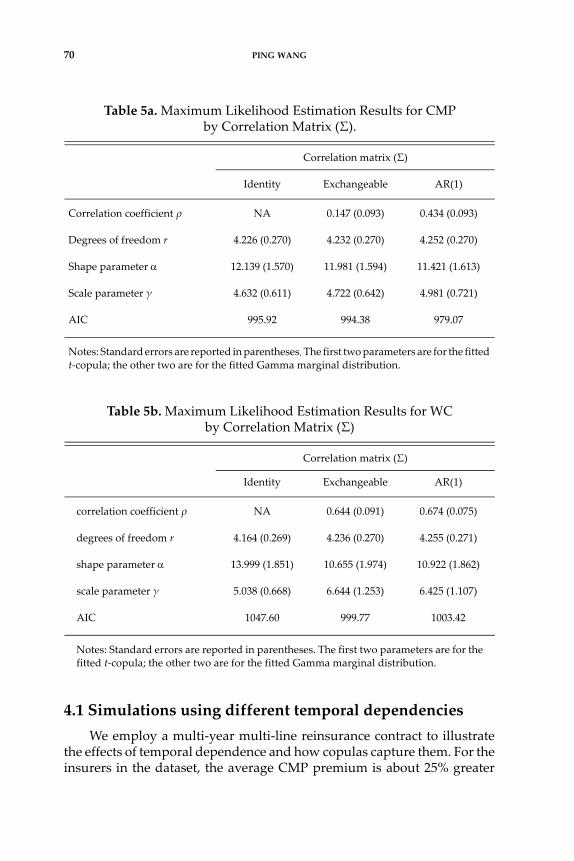
Descriptive statistics presented in Table 7 confirm what we haveobserved in Figure 3. The distribution of Total Loss produced by an inde‐pendence assumption is more symmetric and less volatile compared to thatproduced by assuming copula dependence. From the perspective of thereinsurer, the magnitude of the right tail (“exceedance probability,” a keyterm in catastrophe modeling) is the most significant issue. Table 7 showsthat the maximum value of Total loss under copula dependence is 12%larger than that when temporal independence is assumed.
Fig. 3. Kernel density of Total loss using different dependence assumptions.Note: The kernel density of the Total loss variable using copula dependence is depicted by thesolid curve, while the dashed curve displays the kernel density under the temporal indepen‐dence assumption. The areas to the right of the line with arrows at Total loss of 595.8 indicatethat the distribution modeled by copula dependence has a thicker tail than that of thedistribution derived using the temporal independence assumption.
74 PING WANG
Although Value‐at‐Risk (VaR) is a measure commonly used to evaluatethe potential loss of a high‐risk asset or portfolio, it is not coherent in theterms defined by Artzner (1999). Recently, a robust, convenient, and coher‐ent measure, conditional tail expectation (CTE), is quickly becoming apreferred measure for portfolio and asset assessment. CTE is especiallyuseful in quantifying long‐tail risk exposures. Manistre and Hancock(2005) summarize the properties of CTE that make it preferable to tradi‐tional Value‐at‐Risk measure. Tables 8a and 8b present the values of bothVaR and CTE at high percentages to further study the differences in thedistributions of the Total loss variable generated by assuming either copuladependence or temporal independence. To demonstrate the effects on riskmeasures of (i) an increasingly skewed distribution, and (ii) an increasinglydependent structure, two more sets of simulations were run and theassociated VaRs and CTEs were calculated. Specifically, Table 8a displaysthe risk measures for three different temporal dependence structures:independence, dependence modeled by a t‐copula with all parameters
Table 8a. VaR and CTE of Total Loss (in $ millions) Using Fitted Marginal Distributions, by Different Dependence Structures
Percentage (%)
Copula dependence,ρ = 0.3 for both WC
and CMP
Copula dependence,ρ = .64 for WC and
.43 for CMP Independence
VaR CTE VaR CTE VaR CTE
99.5 698.080 732.394 683.025 719.132 631.948 655.245
99 660.840 704.613 649.589 692.477 610.872 637.249
95 595.420 637.094 587.857 627.161 568.998 595.911
90 563.536 607.559 557.461 599.084 545.428 576.016
Table 7. Descriptive Statistics of Total Loss (in $ millions)
Mean MedianStandard deviation Minimum Maximum
Copula dependence 468.905 463.548 73.365 194.783 812.173
Independence 469.124 467.057 58.264 293.606 724.812

RISK MODELING REINSURANCE USING COPULAS 75
being estimated (ρ = .6443 for WC and .4339 for CMP), and dependencemodeled by a t‐copula with arbitrarily reduced correlation coefficients (ρ= 0.3 for both WC and CMP). Table 8b illustrates the effect of introducingmore skewed marginal distributions to the models. In this table, the fittedmarginal Gamma distribution was modified by halving the shape param‐eter and doubling the scale parameter.
The observed values of both VaR and CTE support the notion that iftemporal independence is assumed when analyzing the underlying lossvariable of a multi‐line, multi‐year reinsurance contract, risk embedded inthe product tends to be underestimated. As a result, decisions of asset‐liability matching and capital management based on the risk assessmentare likely to be inadequate, exposing the reinsurer to greater financial risk.
Consider the case where the stop‐loss threshold is 80% of totalpremiums. Under this scenario, the reinsurance coverage will be triggeredwhen the aggregate loss of the primary insurer exceeds $595.8 million. Of10,000 simulations of Total loss based on the assumption of temporalindependence, 196 are greater than the threshold, indicating that thereinsurer should expect claims from the primary insurer at a frequency ofapproximately 2%, or one every fifty years. The aggregate payments madeby the reinsurer as a result of exceeding the threshold 196 times is $4,805million, leading to an average expected claim of $24.5 million.
However, when 10,000 simulations were run assuming the fitted cop‐ula dependence (ρ = .64 for WC and .43 for CMP), 495 exceeded thethreshold, yielding an expected reinsurer claim frequency of approxi‐mately 5%, or one every twenty years. The average amount of expected
Table 8b. VaR and CTE of Total loss (in $ millions) Using More Skewed Marginal Distributions, by Different Dependence Structures
Percentage (%)
Copula dependence, ρ = 0.3 for both WC
and CMP
Copula dependence, ρ = .64 for WC; .43 for
CMP Independence
VaR CTE VaR CTE VaR CTE
99.5 811.688 861.940 791.004 842.621 706.633 749.519
99 750.098 819.671 734.900 801.558 678.013 720.574
95 649.925 714.136 639.972 699.952 612.885 656.072
90 602.488 669.178 594.584 657.253 577.920 624.697

76 PING WANG
claims is $41.71 million, 70% higher than the estimation based on temporalindependence assumption. When the correlation coefficients in the copulacorrelation matrix are reduced, the CTEs and VaRs are still significantlylarger than those derived under the independence assumption, thoughonly slightly smaller than the case of the fitted dependence structure.
Comparing the results in both tables, we note that an increasinglyskewed marginal distribution (Table 8b) also has significant influences onthe risk measures, even after controlling for the dependence structure. Forexample, when the dependence structure is the fitted copula model, theCTE calculated using the fitted marginal Gamma at 99.5% significance levelis $732.394 million. When the marginal Gamma’s skewness coefficient isincreased to 1.414 times the fitted value,2 the CTE jumps to $861.940 million.
5. SUMMARY AND CONCLUDING REMARKS
The relationships between loss variables underlying a multi‐year,multi‐line reinsurance contract are complicated since correlations may bepresent in two dimensions: from year to year and/or across differentbusiness lines. Thus, modeling of the underlying loss variables of thereinsurance contract presents a challenge. While the reinsurer of the multi‐year, multi‐line agreement may be able to choose two or more independentbusiness lines for the purpose of risk diversification, it is nearly impossibleto remove all of the temporal dependence of annual loss experience. Theassumption of temporal independence is likely to result in a misidentifica‐tion of the distribution of the underlying loss variables, potentially leadingto a significant under‐estimation of the risk embedded in the reinsuranceproduct.
This paper applies copulas to the modeling of the multi‐year depen‐dencies of losses arising from each business line covered by the reinsurancecontract, simulates random draws from multivariate loss ratios repre‐sented by the copulas, and demonstrates the effects of temporal dependen‐cies on some risk measures of a multi‐year, multi‐line reinsurance contract.
As a matter of fact, the same approach can be readily extended toaddress simultaneously both temporal dependencies and dependenciesamong lines of business. Specifically, the correlation matrix (Σ) in Section3.3 can be extended to a 10 by 10 matrix in which the two sub‐matrices onthe diagonal capture the temporal dependencies for CMP and WC respec‐tively (as illustrated), while the two sub‐matrices off the diagonal model
2 This is achieved by halving the shape parameter and doubling the scale parameter so thatthe mean value remains unchanged.

RISK MODELING REINSURANCE USING COPULAS 77
the dependencies among the two lines of business. See, for example, Shiand Zhang (2011) for a similar application.
The idea proposed provides an improved and convenient tool formodeling the risk of alternative risk transfer products. If individual insurercharacteristics associated with the loss ratio variable can be identified, theanalysis can be extended to the application that incorporates covariates inorder to better predict that insurer’s loss distribution.
ACKNOWLEDGEMENTS
The Society of Actuaries (through the Committee on KnowledgeExtension Research) and the Actuarial Foundation (through the ActuarialEducation and Research Fund) provided funding to support this research.The author is grateful for the support.
REFERENCES
Artzner, P (1999) Application of Coherent Risk Measures to Capital Requirementsin Insurance, North American Actuarial Journal 3, No. 2: 11–25.
Cherubini, U, E Luciano, and W Vecchiato (2004) Copula Methods in Finance,London, UK: John Wiley and Sons Ltd.
Culp, CL (2006) Structured Finance and Insurance: The ART of Managing Capital andRisk, New York: Wiley.
Eling, M and D Toplek (2009) Modeling and Management of Nonlinear Dependen‐cies—Copulas in Dynamic Financial Analysis, Journal of Risk and Insurance 76 (3):651–681.
Embrechts, P, F Lindskog, and A McNeil (2001) Modeling Dependence with Copulasand Applications to Risk Management. Available at www.risklab.ch/ftp/papers/DependenceWithCopulas.pdf
Frees, EW and E Valdez (1998) Understanding Relationships Using Copulas, NorthAmerican Actuarial Journal 2, No. 1: 1–25.
Frees, EW, P Shi, and E Valdez (2009) Actuarial Applications of a HierarchicalInsurance Model, Astin Bulletin 39 (1): 165–197.
Frees, EW and P Wang (2005) Credibility Using Copulas, North American ActuarialJournal 9, No. 2: 31–48.
Frees, EW and P Wang (2006) Copula Credibility for Aggregate Loss Models.Insurance: Mathematics and Economics 38: 360–373.
Klugman, S, H Panjer, and G Willmot (2008) Loss Models, 3rd edition, Hoboken, NJ:John Wiley & Sons.
Manistre, BJ and GH Hancock (2005) Variance of The CTE Estimator, North Amer‐ican Actuarial Journal 9, No. 2: 129–156.
Nelsen, RB (1999) An Introduction to Copulas, Lecture Notes in Statistics 139,Springer.

78 PING WANG
Shi, P and W Zhang (2011) A Copula Regression Model for Estimating FirmEfficiency in the Insurance Industry, Journal of Applied Statistics, Vol. 38, Issue(10): 2271–2287.
Swiss Re (2004) Understanding Reinsurance: How Reinsrers Create Value and ManageRisk, available at www.swissre.com.
Swiss Re (2011a) Essential Guide to Reinsurance, available at www.swissre.com.Swiss Re (2011b) Sigma, No. 2, World Insurance in 2010, available at
www.swissre.comVenter, G, J Barnett, R Kreps, and J Major (2007) Multivariate Copulas for Financial
Modeling, Variance 1, No. 1: 103–119.

RISK MODELING REINSURANCE USING COPULAS 79
APPENDIX A
Predictive Distribution Using t-Copula
Frees and Wang (2005) present a brief review of the t‐copula and itsrelated predictive distribution. In this appendix, the predictive distributionis extended to multivariate case for the completeness of the paper.
A.1 The multivariate t-distribution
Suppose that (N1, …, NT) has a joint standardized multivariate normal
distribution with correlation matrix Σ. Also assume that follows a Chi‐
square distribution with r degrees of freedom and is independent of (N1,…,
NT). Then, the joint distribution of { } consti‐
tutes a multivariate t‐distribution with r degrees of freedom. One propertyof this distribution is that each marginal distribution is a t‐distribution withr degrees of freedom, denoted by Tr. Moreover, subsets have the same
family as the joint distribution. Thus, if we assume that (Z1, …,ZT,…,ZT+m)
follows a multivariate t‐distribution, then (Z1, …, ZT) also has a multivariate
t‐distribution. The joint probability density function of (Z1, …, ZT) is
(A.1)
where z = (z1, …, zT)´.
A.2 The t-copula
Multivariate t‐copula is a function defined for all
by , where FZ is the cumulative dis‐
tribution function associated with the probability density function fZ of
multivariate t‐distribution. From equation (A.1), the corresponding prob‐ability density function is
, where tr(.) is the prob‐
ability density function associated with Tr, a univariate t‐distribution with
r degrees of freedom. The conditional density function using copula is
r2
Zt Nt r2 r
1–t 1 T,,=,=
fz z r ,; r T+ 2
r T 2 r 2 1 2----------------------------------------------------- 1
1r---z' 1– z+
=
u1 u2 uT,,, 0 1, T
C u1 uT,, Fz Tr1– u1 Tr
1– uT ,, =
c u1 uT,, fz Tr1– u1 Tr
1– uT ,, 1
tr Tr1– ut
----------------------------
t 1=
T
=

80 PING WANG
.
A.3 Predictive density
If we assume the distribution function of can
be modeled by a copula, we have .
The related joint density function is given by
, where
and Fit(yit) = Fit is the corresponding distribution
function. Thus, the predictive distribution for the period is
where , and .
APPENDIX B
Simulation of multivariate variable using t-copula
For a 3‐dimensional multivariate whose marginal distributions are and joint distribution is represented by a t‐copula with r degrees
of freedom and correlation matrix , the simulation procedure follows.
• Find the Cholesky decomposition A of
• Simulate three i.i.d z1, z2, z3 from standard normal N(0,1) to form
c uT 1+ uT m+ u1 uT,,,,
fz Tr1– uT 1+ Tr
1– uT m+ Tr1– u1 Tr
1– uT ,,,, 1
tr Tr1– uT 1+
------------------------------------- .
t 1=
m
=
Yi Yi1 Yi2 Yi3 YiT,,,, '=
Fi yi1 yiT,, C Fi1 yi1 FiT yiT ,, =
fi yi1 yi T,,, c Fi1 Fi2 FiT,,, f yit it,
t 1=
T
=
fit yit fit f yit it, = =
T 1 T m+,,+
fi yi T 1+, yT m+ yi1 yiT,,,, fi yi1 yi T, yi T m+,,,,
fi yi1 yi T,,, ------------------------------------------------------=
c Fi1 FiT Fi T m+ ,,,,, c Fi1 FiT,,
---------------------------------------------------------------- f yi T t+, i T t+,,
t 1=
m
=
fz vi T 1+, vi T m+,,, vi1 viT,, 1tr vi T s+, ------------------------- f yi T t+, i T t+,,
t 1=
m
s 1=
m
=
vit Tr1– Fit yit = t 1 T m+,,= vi vi1 viT,, '=
F1 F2 F3,,
z z1 z2 z3, '=

RISK MODELING REINSURANCE USING COPULAS 81
• Simulate a variate s from independent of z, where is Chi-squaredistribution with r degrees of freedom
• Set
• Set
• Set for , where denotes the cumulativedistribution function of univariate t-distribution with r degrees offreedom
• represents a random draw.
APPENDIX C
Companies in the Data Set
The market share of each company in the list in both lines of business(commercial multiple perils and workers compensation) was in the top 200in year 2006. The time period observed is 2000–2004, corresponding to Year1 through Year 5 in the analysis.
Cincinnati Insurance Co. Vigilant Insurance Co
Tokio Marine & Nichido Fire Ins Co Continental Casualty Co
Federated Mutual Insurance Co Country Mutual Insurance Co
Frankenmuth Mutual Insurance Co Farmers Insurance Exchange
Harleysville Mutual Insurance Co Hanover Insurance Co
Hastings Mutual Insurance Co Secura Insurance A Mutual Co
GuideOne Mutual Insurance Co New Hampshire Insurance Co
Public Service Mutual Insurance Co Ohio Casualty Insurance Co
Society Insurance Westfield Insurance Co
Church Mutual Insurance Co Pekin Insurance Co
Auto Owners Insurance Co General Casualty Co of Wisconsin
American Family Mutual Insurance Co State Farm Fire and Casualty Co
Hartford Fire Insurance Co Charter Oak Fire Insurance Co
Central Mutual Insurance Co Utica Mutual Insurance Co
Federal Insurance Co Erie Insurance Exchange
Pacific Indemnity Co Hartford Casualty Insurance Co
r2 r
2
y Az=
u r s y=
ti Tr ui = i 1 2 3,,= Tr
x1 x2 x3,, ' F11– t1 F2
1– t2 F31– t3 ,, '=