Traineeship

Polytecnico di Bari, Italy

Modeling of pulley based CVT systems: Extension of the CMM model with bands-segment

interaction Dct nr: 2007.024

J.F.P.B. Diepstraten

Coach:

Dr. Ing. G. Carbone

Dr. P.A. Veenhuizen

January 2007

2

Contents

Contents....................................................................................................................................................2

Introduction ..............................................................................................................................................3

1. Introduction to CVT systems................................................................................................................5

1.1 Pulley Based Transmission.............................................................................................................5

1.1.1 Metal Pushing V-belt...............................................................................................................6

1.1.2 Metal V-chain ..........................................................................................................................6

2. Existing Models....................................................................................................................................8

2.1 Assumptions ...................................................................................................................................8

2.2 Mechanical Model ..........................................................................................................................8

2.3 Pulley Deformation.........................................................................................................................9

2.4 Momentum Equation .................................................................................................................... 10

2.5 Comparison with other models ..................................................................................................... 11

2.6 Simplified and Dimensionless equations...................................................................................... 13

3. Band Segment Interaction .................................................................................................................. 15

3.1 Assumptions ................................................................................................................................. 15

3.2 Geometrical model ....................................................................................................................... 15

3.3 Continuity Equation...................................................................................................................... 17

3.4 Forces equilibrium........................................................................................................................ 17

3.5 Dimensionless equations .............................................................................................................. 19

3.6 Influence of clearance between the segments ............................................................................... 19

3.7 Parameters .................................................................................................................................... 21

3.8 Driving Pulley .............................................................................................................................. 22

3.9 Driven Pulley................................................................................................................................ 28

3.10 Verify distribution of the kinematical strain............................................................................... 35

4. Future Work ....................................................................................................................................... 40

Conclusions ............................................................................................................................................ 41

Literature list .......................................................................................................................................... 42

3

Introduction

Nowadays the car has become the most used transportation application in the world. From some

estimation there are nowadays almost 1000 millions registered vehicles over our entire planet [Ref: 1],

and this number is still rising. This enormous number of cars has great influence on our environment.

The exhaust gases are filled with toxic gases and particles, like nitrogen oxides and sulphur oxides, and

also not directly poisonous gases like carbon dioxide and vapour. The toxic gases contribute to smog

problems in big cities, and other air pollutions, this leads to all kinds of health problems. Carbon

dioxide has a significant contribution to the greenhouse effect. This extended greenhouse effect leads to

global warming and climate change we are dealing with.

Different solutions are thought of to solve this problem. In the late seventies vehicles became equipped

with catalytic converters, these converters reduce the toxic gases in the vehicle exhaust. Also the

internal combustion engines have been further developed to produce less exhaust gases. These

applications contributed to a decrease of the harmful exhaust gases.

In the last decade also other solutions have been thought of. Some of them exist of replacing the

combustion engine by a fuel cell, or a combination of the combustion engine with a battery, called

hybridization. Another solution is topology change of the drive train. For a few years a sixth gear has

been added to the conventional gear box, this to reduce the rotating speed of the engine at high vehicle

speed to reduce the exhaust gases. One more solution is the use of a continuously variable

transmission, CVT. This transmission is able to provide infinite gear ratios between two constraint

limits, without the use of any clutch to disengage the engine from the drive line. By this property the

combustion engine can be driven in its optimal working point, the engine speed does no longer depend

on the drive line, because this can be freely chosen due the presence of the CVT. This means the

combustion engine always can be used in its working point at which it delivers the most power. A well

chosen engine speed also leads to a minimum of exhaust gases.

This last solution is an interesting one. A CVT can be easily used in place of classical transmission in a

normal car. The drive train must be replaced, but the combustion engine and other energy storage

devices can keep the “old” configuration. So the already used lay out of the car does not have to be

fully changed, as instead is the case of fuel cells or hybrid engines.

Further more it has been estimated that fuel reduction of 10% could be obtained using a CVT in

comparison with a manual shitted gear box [Ref: 2]. This may significantly reduce the above

mentioned environmental problems concerning fossil fuels.

Also the driveability of a vehicle equipped with a CVT is very good. The driver does not have to

change gear, and by doing this lose his attention on the road. Moreover the comfort rises, because the

sudden (de)acceleration during shifting disappears. Torque disengagement will also disappear, because

no clutch is used during normal driving.

The CVT seems a good transmission to place in modern vehicles. But there are still some problems. A

CVT is a complicated transmission and must be controlled by a hydraulic system managed by an

electronic control unit (ECU). This control still must be further optimized and investigated, this is

necessary to obtain the lowest fuel consumption and emission, and highest driveability and comfort. At

this time the control and control strategy are not to be called optimal. The hydraulic clamping forces

determine the transmission’s efficiency and maximum torque that is transmitted. The timing and size of

these hydraulic forces must be further investigated to reach the optimal desired working point.

Another problem is the question wetter the consumer is prepared to buy this new transmission, or not.

Especially in Europe the manual shifted gear box has a big market share, about 80% of all new

produced cars are equipped with manual gear boxes. In Japan the CVT has already a marking share of

20% and the American market is very promising for the CVT [Ref: 3]. But then the question still

remains, will there be enough demand for CVT vehicles?

To be able to determine the behaviour of the CVT transmission different approaches exists, one

mathematical models, multi-body models and FEM models. In this paper the mathematical model,

especially the CMM model, is investigated. The CMM model is derived by Carbone, Mangialardi and

Mantriota from the Polytecnico di Bari, Italy. This mathematical model has been compared with

experiments done at the Technical University of Eindhoven, the Netherlands. This comparison showed

some inequalities between model and experiments. This can be seen in figure 1. In this figure the

geometric speed ratioτ (x-axis) is compared with the clamping force ratio DNDR SS / (y-axis). The fat

line represents the CMM model, the thin lines the results of the experiments.

4

Figure 1: Comparison CMM model and experiments

In this paper a start is made to derive a solution that can cancel these inequalities. The CMM model

will be extended with some equations, in such a way that a better approximations can be made with

respect to the experiments. Because of time limits the exact new model is not derived, but sufficient

equations will be derived to complete the new model.

In the first chapter of this paper a closer look will be taken to different kinds of CVT transmission like

belt CVTs and chain CVTs. In the second chapter the CMM model concerning belt and chain CVTs is

presented and after this in the third chapter the extended version of this model is derived and some

results of this extended version are presented. The last chapter deals with some recommendations about

continuation of the research in such a way that the new model can be derived.

5

1. Introduction to CVT systems

In the first chapter is explained why to use a Continuously Variable Transmission (CVT) as drive train

in a vehicle. In this chapter a brief history will be given, an overview of the commercial applied CVTs

and how they work and its advantages and disadvantages.

Leonardo da Vinci was said to be the first one who thought about a CVT system around 1490. But

when the invention of the car was a fact at the end of the 19th century, CVT became a true issue. The

first CVT patent dates from 1886. The first commercial CVT equipped vehicle was produced in 1958

by DAF (van Doorne Automobiel Fabriek), in the Netherlands, this factory was set up by Hub van

Doorne in 1928. He invented the Variomatic CVT, this is based on a double V-belt system. The

transmission was placed on the rear wheels and the drive train did not contain a differential gear. The

system and the produced car can be seen in figure 1.1

Figure 1.1: Variomatic; layout and produced car

This transmission first could only be used for low-powered cars, 600cc, after some improvements this

raised to 1400cc. About 1,2 million vehicles were equipped with the Variomatic [Ref: 4].

After the launch of the Variomatic different types of CVTs are produced by different companies.

Two different commercial applied CVTs exist, the pulley based CVT and the toroidal CVT. Some

other CVTs exists, but they are only used for research, prototype or at very low scale.

1.1 Pulley Based Transmission The pulley based transmission is the transmission in the above mentioned Variomatic created by DAF.

It consists of two pulleys connected with a V-shaped belt, this kind of CVT is therefore also called the

V-belt CVT. The pulley that is connected to the engine is called the driving or primary pulley, the other

pulley is connected to the wheels and is called the driven or secondary pulley. By changing the axial

position of the moveable sheave of each pulley the pitch radius of the belt is changed and in turn the

transmission ratio is modified, this is shown in figure 1.2.

Figure 1.2: Concept of V-belt CVT’s

6

In the left figure the transmission is in its lowest gear and in the right figure in its highest gear. One

sheave of each pulley is connected with a hydraulic circuit, these controlled sheaves are on the opposite

side of the belt. With the hydraulic circuit the clamping force on each pulley can be varied, by

modifying the clamping force the radius of each pulley can be changed, and so the transmission ratio.

This kind of transmission can provide a speed ratio from 0.4 up to 2 or even higher [Ref: 5].

Two different types of V-belts are used in CVT’s; the metal pushing V-belt and the metal V-chain.

1.1.1 Metal Pushing V-belt The push belt is an enhanced version of the DAF Variomatic. It was invented again by Hub van

Doorne, and it consists of two series of thin metal bands, which hold together a number of wedge-

shaped steel blocks. This belt is manufactured by VDT, Van Doorne Transmission. When the blocks

are compressed, by pushing, they act as one single rigid column, by this it is possible to transmit torque

from one pulley to the other one. In figure 1.3 the construction of a metal pushing V-belt is shown.

Figure 1.3: Construction of metal pushing V-belt

A belt consists of two band-sets with 9 to 12 metal bands. These bands give to the belt its flexibility

and provide the necessary tensile strength. The number of blocks or segments, depending on the length

of the belt, is approximately 400. A segment can have different measures and sizes. A larger block,

which means a larger contact area with the sheave, decreases the contact pressure at higher torque load.

Size and measures of the segments are optimized for its application.

The main failure mechanisms are related to over speeding, misalignment and insufficient lubrication

[Ref: 6].

The metal push V-belt is used as drive train by companies like Fiat, Ford, Subaru and Nissan. It was

also applied in the Formula 1, developed by Williams and VDT. It was a prototype, but the FIA,

Fédération Internationale de l’Automobile, banned the CVT from single-seat racing.

1.1.2 Metal V-chain The metal V-chain CVT transmits the torque through a tension difference between two chain strands.

Links and rocker joint pins are available to transfer the chain tension. In figure 1.4 the metal V-chain

and the layout of this transmission are shown. The chain is a Luk type chain belt, and is applied in the

Audi A6, 2.8L Multitronic.

7

Figure 1.4: Metal V-chain and layout

Instead is the push belt, the chain can only transmit torque by tension in the chain, not with pressure.

The chain consists of a number of chain elements depending on the size of the chain variotor. The main

failure mechanism is fatigue of the link plates, and the elements that contact the sheaves, pin or strut.

The fatigue is mostly due to tension in the belt and a little less to articulation [Ref: 6].

8

2. Existing Models

In chapter 1 it was made clear that for obtaining the right variation of speed ratio, understanding the

behavior of the metal belt CVT is crucial to predict the needed clamping force. In this chapter the

CMM model of the metal belt CVT is presented.

Experiments made clear that two different shifting behaviors of the metal belt CVT exist. The first

mode is the creep mode, this mode is characterized by the fact that the ratio of the clamping force

acting on the primary pulley to that acting on the secondary pulley is mainly influenced by the rate of

change of the speed ratio and by the tangential velocity of the belt.

The slip mode takes place during fast shifting maneuvers and is characterized by the fact that the above

mentioned ratio of the clamping forces is neither influenced by the magnitude of the rate of change of

the speed ratio nor by the tangential velocity of the belt. These characteristics can be shown by using

the CMM model.

This model [Ref: 7], made up by Carbone, Mangialardi and Mantriota, uses kinematical and

geometrical relations and also takes into account the pulley deformation. The model will be compared

with another model, a Multi-Body model.

2.1 Assumptions The model that will be presented is derived by making some assumptions and simplifications.

The metal belt is considered as a continuous body, with locally rigid motion. This means there is no

longitudinal and transversal deformation, i.e. the belt is considered to be an inextensible strip with zero

radial thickness and infinite axial stiffness. Furthermore the bending stiffness of the belt is neglected.

The considered Coulomb friction, with the friction coefficient µ, acting between the segments and the

pulleys, has a constant value. The deformation of the pulley will be described on the basis of Sattler’s

model.

In the derivation of the model second order terms will be neglected.

2.2 Mechanical Model In figure 2.1 the entire CVT variator is shown, the driving (primary) and driven (secondary) pulley are

presented. In figure 2.2 the kinematical and geometrical quantities involved are shown.

Fig 2.1: CVT scheme Fig 2.2: Kinematical en geometrical

quantities involved. (a) planar view,

(b) 3D view

Explanation of the parameters in these figures:

ψ: sliding angle

γ: complementary angle of ψ; ψπγ −=− 2/

θ: angular coordinate

9

r: radial coordinate

ρ: radius curvature

φ: slope angle

τ: tangent unit vector

n: corresponding normal unit vector of τ

er, eθ: radial and circumferential unit vector

vs: sliding velocity and its components r& and srω

β: pulley half-opening angle

βs: pulley half-opening angle in the sliding plane

From figure 2.2 the following geometrical equations can be derived.

( )θ

ϕ∂

∂=

r

r

1tan [2.1]

( )

δθϕ

δcos

rl = [2.2]

( )

∂

∂−=

θ

ϕϕ

ρ1

cos1

r [2.3]

( ) ( ) ( )ψββ costantan =s [2.4]

( )ψω tanrr s&=⋅ [2.5]

With:

ωs: local sliding angular velocity of the belt; ωω −Ω=s

Ω: local angular velocity of the belt

ω: pulley rotating velocity

δl: length of a material element of the belt

δθ: angular extension of the same material element

After taking the material time derivative of equation [2.2], this becomes:

( ) θθ

ϕϕ ∂∂

++=∂∂ Dt

D

r

rl

Dt

D

l

1tan

1&

& [2.6]

Neglecting elongation of the belt, variation of the pulley rotating velocity in tangential direction and

the slope angleϕ , the continuity equation of the belt can be written into:

0=∂

∂+

θ

ωs

r

r& [2.7]

2.3 Pulley Deformation To calculate the actually path of the belt (the radial position of the belt), transversal deformation and

pulley deformation must be known. Experiments made clear that belt transversal deformation does not

contribute to radial differentiation in the position of the belt. On the contrary, pulley deformation can

vary the radial position of the belt between 0.1 to 1 mm. So belt transversal deformation is neglected

and only pulley deformation is taken into account [Ref: 7]. In figure 2.3 the pulley deformation is

shown.

10

Figure 2.3: Pulley deformation

The actually pulley deformation is described by the using the Sattler’s Formulas. They describe the

varying groove angle β and the axial displacement u of the pulley.

+−

∆+=

2sin

20

πθθββ c [2.8]

( )0tan2 ββ −⋅⋅= Ru [2.9]

With:

0β : groove angle in undeformed situation

∆ ≈ 10-3: amplitude of the sinusoid

cθ : center of the wedge expansion

R: pitch radius of the belt, the distance from the pulley axis that the belt would have if the

pulley sheaves were rigid.

The local radial position can be calculated by:

2

tantan 0

uRr −⋅=⋅ ββ [2.10]

Taking the time derivative of the above equation the radial velocity can be calculated.

( )cr Radt

dRv θθω −∆+= sin [2.11]

where ( ) ( )00

2 2sin/cos1 ββ+=a

2.4 Momentum Equation The equilibrium of the belt involves the tension of the belt (F), the linear pressure acting on the belt

sides ( p ), the friction force (af ), and inertia, centrifugal, force of the belt element (

2)( R⋅ωσ ). This

is visualized in figure 2.4. The friction force pfa ⋅= µ

11

Figure 2.4: Forces acting on belt

σ = mass density

F = T – P ; the net tension of the belt

T: tension of the band

P: compressive forces between metal segments

A number of assumptions are made to calculate the equilibrium. At first it is possible to calculate the

local angular acceleration θ& of the considered belt’s material element with the pulley’s angular

velocity ω. Secondly from equation [2.3] follows Rr ≈≈ρ , therefore all these three parameters are

written as R. Thirdly the term R&& is neglected with respect to R2ω , i.e. 12

<<R

R

ω

&&, furthermore also

1<<ϕ . The last assumption is that the belt’s axial and tangential acceleration can be neglected [Ref:

8]. With these assumptions, the two involved equations are:

( )

ψβµβ

ψβµ

θ

ωσ

ωσ coscossin

sincos1

0

22

22 ⋅⋅−

⋅⋅=

∂

⋅⋅−∂

⋅⋅− s

sRF

RF [2.12]

( )ψββ

ωσ

coscossin2 0

22

⋅−

⋅⋅−=

sR

RFp [2.13]

With this last equation it is possible to calculate the center of the wedge expansion cθ as:

( ) ( )

( ) ( )∫

∫=

α

α

θθθ

θθθ

θ

o

oc

dp

dp

cos

sin

tan [2.14]

2.5 Comparison with other models The determined CMM model will be compared with another model, this is a Multi-Body model derived

by Srnik and Pfeiffer [Ref: 9]. The results are obtained during steady-state behaviour, in the CMM

model this means the parameter A from equation [2.25] has the value zero. Furthermore the wrap angle

is 180° and the groove angle β0= 10°. In the figures below, figure 2.5 and 2.6, the results are shown for

the driving and driven pulley.

The driving pulley has a ξ value of 0.35 and the driven pulley a value of 1/0.35. ξ represents a ratio

between the force at the exit and at the entrance of the pulley, see equation [2.33]. In the figures the

12

relation between sliding angle γ and angular coordinate α is presented; here is 2/πψγ −= . In the

driving pulley the angular coordinate α is given as 2/, πθα += DRDriveI and in the driven pulley as

2/, πθα −= DNDrivenI .

Figure 2.5: Result driving pulley Figure 2.6: Result driven pulley

a) Multi-Body

b) CMM

---) flexible pulley

) rigid pulley

From these figures can be concluded that the CMM model and the Multi-body produce almost similar

behaviour, this is off course good. Also must be concluded that pulley deformation has a large

influence on the sliding angle.

In figure 2.7 the tensile forces on one chain link are shown during one revolution, and in figure 2.8 the

normal forces are presented. The calculation is done under the above mentioned condition. The friction

coefficient µ has a value 0.1, and ξ has a value 0.35. Furthermore the minimal tension force in the belt

is 1.6 kN.

Figure 2.7: Tensile forces Figure 2.8: Normal forces

a) Multi-Body

b) CMM

The agreement is quite good between both models. Some differences exist in the normal forces at the

driving pulley, but it is only a small error.

13

So the CMM model is a good model to describe the behaviour of a CVT, and can be used to understand

its performance.

2.6 Simplified and Dimensionless equations To be able to calculate the force acting on the belt and the pulley pressure the equations have to be

rewritten into dimensionless equations. These equations will be needed in the next chapter.

To simplify equations [2.1 and 2.7], consider 1<<ϕ . The equations become:

θ

ϕ∂

∂=

r

r

1 [2.15]

0=∂

∂+

θθv

vr [2.16]

All the previously derived relations can be rephrased in dimensionless form, using the following

dimensionless quantities:

R

Rw

ω

&= [2.17]

( )

0

2

0

cos1

2sin

β

β

+∆=

wA [2.18]

( )

0

2

0

cos1

2sin1~

β

β

ω +∆=

r

rvr

& [2.19]

( )

0

2

0

cos1

2sin1~

β

β

ω

ωθ

+∆= sv [2.20]

22

0

22

RF

RF

σω

σωκ

−

−= [2.21]

22

0

~

RF

Rpp

σω−

⋅= [2.22]

In equation [2.28] F0 is the tension force of the belt at the entry point of the pulley, 0=θ . Equation

[2.5] can be written into:

( )rv

v~

~tan θψ = [2.23]

And [2.23] means:

0~

~ =+δθ

δ θvvr [2.24]

From equation [2.11] can be concluded that:

+−−=

2cos~ π

θθ cr Av [2.25]

Equation [2.12, 2.13 and 2.14] can be written into:

ψµψββ

ψµ

θ

κ

κ coscostan1sin

sin1

2

0

2

0 −+

⋅=

∂

∂ [2.26]

2coscostan1sin

costan1~2

0

2

0

2

0

2κ

ψµψββ

ψβ

−+

+=p [2.27]

14

( )

( )∫

∫

∂⋅

∂⋅

=α

α

θθ

θθ

θ

0

0

cos~

sin~

tan

p

p

c [2.28]

Combining [2.24 and 2.25] result in:

−

−−= cAvv θ

θθθθθ

2sin

2sin2~~

0 [2.29]

Equation [2.23] can be written into:

+−−

−

−−

=

2cos

2sin

2sin2~

tan0

πθθ

θθθ

θ

ψθ

c

c

A

Av

[2.30]

To solve these set of equation the following boundary conditions exist:

00

~~θθθ vv =

= [2.31]

10

==θ

κ [2.32]

22

1

22

2

RF

RF

σω

σωξ

−

−= [2.33]

The last parameter ξ is the ratio between the belt tension force at the exit and the entry point of the

pulley.

With a given parameters A and ξ the other parameters can be calculated.

15

3. Band Segment Interaction

As stated in the introduction the presented CMM model from chapter 2 showed some inequalities with

performed experiments. In this chapter a possible solution will be given to deal with these inequalities.

The idea is that band segments interaction can be the solution, this kind of interaction is not taken into

account in the standard CMM model. In this chapter an approximation will be presented to handle this

phenomenon.

As stated before the belt consists of two types of components, the bands and the segments. On the

contact face the difference between the velocity of the bands and the segments will play a significant

role, so this velocity should be derived.

After this the tension of the bands will be further analyzed, the tension is influenced by the above

mentioned velocity. The obtained equations will be added to the CMM model from chapter 2, and

some results will be presented.

3.1 Assumptions Besides the assumptions in the last chapter, other assumptions are considered to derive the equations.

The segments and the bands can slide with respect to each other, i.e. they can have different velocities.

At the contact face between the segments and the bands a Coulomb friction is considered with a

constant friction coefficient. Also we will follow the commonly adopted theory in of elastic beams that

the cross section of the bands and the segments remains plane during motion.

The bands have a tension force T and the segments have pressure force P working on it, in such a way

that the total force F acting on the belt is equal to PTF −= .

The last assumption is that the segments can be separated from each other, this phenomenon will be

further explained in this chapter.

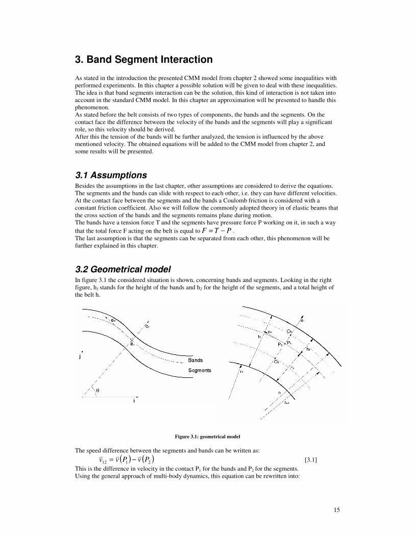
3.2 Geometrical model In figure 3.1 the considered situation is shown, concerning bands and segments. Looking in the right

figure, h1 stands for the height of the bands and h2 for the height of the segments, and a total height of

the belt h.

Figure 3.1: geometrical model

The speed difference between the segments and bands can be written as:

( ) ( )2112 PvPvv −= [3.1]

This is the difference in velocity in the contact P1 for the bands and P2 for the segments.

Using the general approach of multi-body dynamics, this equation can be rewritten into:

16

( ) ( ) θθ ωω ehehOvOvv ZZ

rr22112112 −−−= [3.2]

In this equation ( )iOv is the velocity of the bands or the segments in the point iO . The angular

velocity izω is the angular velocity measured from point Pi, where i stands for 1 representing the bands

and for 2 in case of representing the segments.

The velocity can also be phrased as follow,

( )ii rOv &= [3.3]

Remembering that rii errr

= . Using this, the derivation can be made, which leads to:

( ) θθθ ωωθθ

ehheuerr

v ZZr

rrr2211

22

1112 +−+

∂

∂Ω−

∂

∂Ω= [3.4]

In this equation holds 2211 rru Ω−Ω=θ .

Now taking a more specific look to the term izω . In figure 3.2 this parameter is visualized, αω &=Z1 .

Figure 3.2: Explanation of angles and iZω

From the figure can be made up that:

ϕθα −= [3.5]

This means ϕϕθω &&& −Ω=−= 11Z .

The terms θ∂

∂ ircan be taken together. From figure 3.1 follows:

( )1int1 hrr += [3.5]

( )2int2 hrr −= [3.6]

This means thatθθθ ∂

∂=

∂

∂=

∂

∂ rrr 21.

When the above obtained results are substituted in equation [3.4], it gives:

( ) θθ ϕθ

ehewer

v r

r&

rr++

∂

∂Ω−Ω= 2112 [3.7]

With ( )21int Ω−Ω= rw .

The first term on the right hand side of equation [3.7] is a second order term, 1<<−Ω

ω

ωi, and is

therefore neglected.

17

To calculate ϕ& equation [3.22] is used, remembering thatθ

ϕϕ

∂

∂Ω=& . Second order terms are again

neglected. Substituting this result, leads to:

θθθ

er

R

hewv

rr

2

2

12∂

∂Ω⋅+= [3.8]

The term 2

2

θ∂

∂ rcan be calculated by using equation [2.12]. Using the parameter

)2sin(

cos1

0

0

2

β

β+=a

results in the following equation:

( )[ ] θθθ ehawv c

r−⋅∆⋅Ω⋅⋅+= cos12 [3.9]

3.3 Continuity Equation The continuity equation for both the bands and segments becomes:

0=∂

Ω∂+

θi

ii rr& [3.10]

Now the continuity equation of the segments is subtracted from the continuity equation of the bands.

Consider that θ∂

∂Ω+

∂

∂= i

ii

i

r

t

rr& and that 021 =

∂

∂−

∂

∂

t

r

t

r.

( )

02211 =∂

Ω−Ω∂

θ

rr [3.11]

From this equation it can be concluded that ( )2211 Ω−Ω rr is constant along the arc.

Parameter w can be rephrased into:

( ) ( )212211 hhrrw +Ω−Ω−Ω= [3.12]

Equation [3.12] can also be rewritten into:

( ) ( )

θθθ ∂

Ω∂+−

∂

Ω−Ω∂=

∂

∂21

2211 hhrrw

[3.13]

Because ( )

02211 =∂

Ω−Ω∂

θ

rrand the second order term ( )

θ∂

Ω∂+ 21 hh can be neglected, 1<<

R

h,

the conclusion can be drawn that w is constant along the arc.

3.4 Forces equilibrium A more specific look will be given to the Coulomb friction forces between the belt and the segments. In

figure 3.3 a visualization of the situation is shown. Five forces acting on the belt are considered: two

tension forces on both ends of the section, a normal force and a friction force between the band and the

segments, and a mass inertia force (centrifugal force).

18

Figure 3.3: Visualization of forces on one infinitesimal section dθ of the CVT belt

An assumption is that the belt tension T, is directed in the tangential direction, this means there is no

angle between tension and θer

direction.

R: radius of the belt

T: belt tension

NdF : normal force between band and segments = δθ⋅⋅RPb

with Pb: pressure between band and segments

µdF : friction force between band and segments = δθ⋅⋅⋅=⋅ RPfdFf bN

=f( friction coefficient )

indF : inertia force of the considered band section = δθωσ ⋅⋅⋅⋅ RRb

2

When the equilibrium of the five existing forces is written down the following equation is obtained:

( ) ( ) 0=⋅+−+−+ rinrNd

edFedFedFeTeTrrrrr

θµθθθθθ [3.14]

The first two terms can be combined into one term:

( ) ( ) ( )θ

θθ

θθθθθ ∂∂

∂=−

+

eTeTeT

d

rrr

[3.15]

Equation [3.14] can be written in the tangential direction, θer

, and in the radial direction, rer

, doing this

gives:

0=⋅⋅−∂

∂RPf

Tb

θ [3.16]

022 =⋅⋅+⋅+− RRPT bb ωσ [3.17]

From equation [3.17] follows22

RTRP bb ⋅⋅−=⋅ ωσ . This is substituted in equation [3.16].

( )22RTf

Tb ⋅⋅−⋅=

∂

∂ωσ

θ [3.18]

Using this differential equation the tension of the band can be calculated.

The derivative of tension in the belt is determined by the direction of12v . When

12v is positive, the

θ∂

∂T is positive, and the other way around, when

12v is negative, then θ∂

∂Tis negative. In figure 3.4 a

possible situation that can occur is visualized.

19

Figure 3.4: Possible situation for values of

12v

In the situation above, at two positions the velocity difference between segments and bands,12v , is

zero. This means on two positions the θ∂

∂T will change of direction. The two other possible situations

are when only one point or no point of zero velocity difference exists. Also in these situations the

change of tension is determined by the direction of12v .

3.5 Dimensionless equations To make the equations more understandable the following dimensionless quantities are used.

∆

=ωah

vv 12

12~

[3.19]

∆

=ωah

ww~ [3.20]

22

1

22

RF

RT bbbbb

σω

ωσκ

−

−= [3.21]

With these quantities equation [3.9] is written as:

( )cwv θθ −+= cos~~12

[3.22]

The quotient between the tension in the band at the input and at the output of the pulley is defined as:

22

1

22

2

bbb

bbbb

RT

RT

ωσ

ωσξ

−

−= [3.23]

And equations [3.18] can be rewritten into:

bb f κ

θ

κ⋅=

∂

∂ [3.24]

The segments pressure becomes:

22

1

~

RF

PP

σω−= [3.25]

3.6 Influence of clearance between the segments To calculate the tension at the belt, and pressure on the segments, the model must be expanded with the

influence of clearance between the segments. This subject is investigated in (Ref: 10).

The contact arc exists of two parts, a section where the segments are separated from each other, and

one where the segments are pushed together.

Considering the driving pulley, the above first mentioned section is the first section on the pulley, see

figure 3.5, so here the segments are separated. In this part the only force acting on the belt is the tension

in the bands, caused by the band segment interaction. To calculate this tension equation [3.24] is used.

In the second section the segments are packed together. Two forces exists, the tension in the bands and

20

because the segments are pushed on each other, the pressure on the segments. The total force

becomes PTF −= . Because the total force can be calculated by equation [2.26] and the tension is

known by equation [3.24], also the segments pressure can be calculated.

Figure 3.5: Influence of clearance on driving pulley

At the shock section, at angular coordinate*θ , the segments will collide and come in contact, after this,

a pressure occurs between the segments. The shock section separates the two mentioned phases. The

sliding velocity at the shock section consists of two quantities, one calculated from the kinematical

strain and the other the tangential component of the sliding velocity at*θ . The first component is

calculated by (Ref: 10):

*

**

1 DR

DRDRs

ε

ε

+

−= [3.26]

Withε the kinematical strain of the belt,da

db=ε , db is the distance between two segments and

da is the thickness of one segment. The tangential sliding velocity is calculated with ( ) ( )ψθ tan~ * ⋅rv .

So the sliding velocity at the shock section becomes:

( ) ( ) ( )ψθ

β

βθ tan~

cos1

2sin1~ *

0

2

0*

0 ⋅++

⋅∆

⋅= rDR vsv [3.27]

The pressure at the shock section*P , can be calculated by the following equation (Ref: 10):

( ) 22*** 1 RssP DRDRDR σω⋅+−= [3.28]

When considering the driven pulley, the sections have changed place, as is shown in figure 3.6. In the

first section the segments are packed on each other and in the second section the segments are

separated. The equations used on the driving pulley on each section hold true for the corresponding

section on the driven pulley.

21

Figure 3.6: Influence of clearance on driven pulley

For both pulley holds that in the section where the segments are separated, the total force is equal to the

tension in the bands, therefore can be written from equation [2.26 and 3.24] that in this section holds

true that:

ψµψββ

ψµµ

coscostan1sin

sin

2

0

2

0 SP

SPBS

−+

⋅= [3.29]

With BSµ the friction coefficient between the bands and the segments and SPµ the friction coefficient

between the segments and the pulley. Using the following values the sliding angle ψ can be

calculated. 05.0=BSµ , 09.0=SPµ , deg100 =β . The result can be seen in figure 3.7.

0 1 2 3 4 5 6 7-0.8

-0.6

-0.4

-0.2

0

0.2

0.4

0.6

0.8

psi

Equilibrium k = kb

k

kb

Figure 3.7: Calculation of sliding angle ψψψψ

As can be seen in figure 3.7 two solutions exist for the sliding angle. 0481.01 =ψ and 9937.22 =ψ .

Remembering that with

rv

v~

~tan θψ = the right solution can be picked: the distinguishing must be made

between the driving pulley and the driven pulley. At the driving pulley the section of separated

segments is placed at the entrance of the pulley, in this part the sliding velocity is pointed inwards, so

the sliding angle must be around π. This is the case for2ψ .

At the driven pulley the considered section is placed at the exit of the pulley, the sliding velocity is here

pointed outwards, so the sliding angle must be around 0. This is the case for1ψ . So now the sliding

angle is known in the section where the segments are separated for both pulleys.

3.7 Parameters The calculations are done with the following values of the parameters: πα = rad,

0=A , 05.0=BSµ , 09.0=SPµ , deg100 =β , 2000=ω rpm, 001.0=∆ , 2.1=σ kg/m,

432.0=bσ kg/m, 0540.0=R m, 12=h mm.

Because the driving pulley needs different input parameters to do the calculation than the driven pulley,

the distinguishing is now made between the two pulleys.

22

3.8 Driving Pulley

To do the calculation on the driving pulley three input parameters are needed, these are w~ , the

dimensionless representation of the difference in angular velocity between bands and segments, *θ the

angular coordinate on which the segments come in contact and*ε the kinematical strain in this point.

With given values of these parameters the calculation can be done. The assumption is, as stated before,

that at the entrance the segments are separated and at position*θ the segments are pushed together. By

the use of equation [3.22 and 3.24] the dimensionless tension in the bands can be computed. Because

the kinematical strain at *θ is given,

*ε , the other parameters,*P and 0θv can be calculated. With the

help from equation [3.28] *P , the pressure between the segments in this point, is known, and from

equation [3.27] 0θv can be calculated. From these parameters the dimensionless total force on the belt,

the sliding angle, the pulley pressure and cθ can be calculated in the same way as presented in chapter

2.

To study in which way the different input parameters influence the results of the calculation the

following is done. Two input parameters are fixed at one value, the third parameter is varied in five

different values with equal increasing step size. In this was the influence of this parameter is studied.

The only input parameter that significantly influences the behaviour of the tension in the bands is w~ .

Suitable values for w~ can be approximate from equation [3.22] with setting 12v to zero and an

estimation of cθ . In figure 3.7 the behaviour of bκ is shown for different values of w~ , variation from

1~ −=w up to 6293.0~ =w .

0 0.5 1 1.5 2 2.5 3 3.50.85

0.9

0.95

1

1.05

1.1

1.15

1.2

1.25

Angular coordinate θ [rad]

κb [-]

Dimensionless Tension

wmin = -1

w2

w3

w4

wmax = 0.6293

Figure 3.7: Behaviour for dimensionless tension a varying w~

In case of 1~ −=w the tension is decreasing constantly along the contact arc. In the second case, 2~w ,

two point exists where 12v is zero, the tension is first decreasing, then increasing and at the end for a

second time decreasing. In the last three cases, one point at which 12v is zero exists. First there is a

decreasing tension, and after this an increasing tension. Variation of w~ can therefore cause a rise or a

drop of tension at the exit point of the pulley with respect to the tension at the entrance point.

23

To calculate the other quantities the other two input parameters are fixed, 0025.0* =ε and o70* =θ .

The results are given in figure 3.8, 3.9 and 3.10.

0 0.5 1 1.5 2 2.5 3 3.50

0.2

0.4

0.6

0.8

1

1.2

1.4Dimensionless forces on the belt

Angular coordinate θ [rad]

Fo

rce

s [-]

wmin

= -1

w2

w3

w4

wmax

= 0.6293

Figure 3.8: Dimensionless forces with varying w~

0 0.5 1 1.5 2 2.5 3 3.52.5

3

3.5

4

4.5

5

5.5

6

Angular coordinate θ [rad]

Ψ [ra

d]

Sliding angle

wmin

= -1

w2

w3

w4

wmax

= 0.6293

Figure 3.9: Sliding angle with varying w~

24

0 0.5 1 1.5 2 2.5 3 3.51.5

2

2.5

3

3.5

4Dimensionless pulley pressure

Angular coordinate θ [rad]

Pulle

y p

ressure

[-]

wmin

= -1

w2

w3

w4

wmax

= 0.6293

Figure 3.10: Pulley pressure with varying w~

In figure 3.8 the fat solid lines represent the total force, the thin solid lines the tension and the fat dotted

lines the segments pressure. As can be seen in this figure a segments pressure occurs at *θ . From this

point on the sliding angles rises, causing the total force to decrease, and the segments pressure to

increases.

The sliding angle has expected behaviour; until *θ a constant sliding angle calculated from equation

[3.29], and after this point a big increase until cθ . The small difference is due a different cθ , caused by

a different tension at *θ .

The pulley pressure has also expected behaviour, a more or less constant value until *θ , and after this a

great enhancement until cθ . The difference is the consequence of different cθ and a different values of

the total force, caused by different w~ .

Variation of*ε does not significantly change the behaviour of the tension, the small difference is

caused by a minor difference in cθ . The variation of *ε has the largest influence on 0θv , which

determines an increase or decrease of the total force, *ε is varied from 0.0018 up to 0.0030. The other

two input parameters are fixed at 4905.0~ −=w and o70

* =θ . The results are shown in figure 3.11, 3.12

and 3.13.

25

0 0.5 1 1.5 2 2.5 3 3.5-0.4

-0.2

0

0.2

0.4

0.6

0.8

1

1.2

1.4Dimensionless forces on the belt

Angular coordinate θ [rad]

Forc

es [-]

ε*min

= 0.0018

ε* 2

ε* 3

ε* 4

ε*max

= 0.0030

Figure 3.11: Dimensionless forces with varying*ε

0 0.5 1 1.5 2 2.5 3 3.50

1

2

3

4

5

6

7 Sliding angle

Angular coordinate θ [rad]

Ψ [ra

d]

ε*min

= 0.0018

ε* 2

ε* 3

ε* 4

ε*max

= 0.0030

Figure 3.12: Sliding angle with varying*ε

26

0 0.5 1 1.5 2 2.5 3 3.51

2

3

4

5

6

7

8

9Dimensionless pulley pressure

Angular coordinate θ [rad]

Pulle

y p

ressure

[-]

ε*min

= 0.0018

ε* 2

ε* 3

ε* 4

ε*max

= 0.0030

Figure 3.13: Pulley pressure with varying*ε

In figure 3.11 the same lines represent the same forces as in figure 3.8. In the first case *ε has a very

small value. This causes small values of*P and 0θv . This causes a decrease of the sliding angle, and

therefore a rise of the total force, because of this the segments pressure decreases below zero. This

means the pressure between the segments is first positive, but then becomes negative, with other words,

the segments are after *θ first in contact, but further along the arc the segments are separated again.

This means the pulley is no longer a driving pulley, but a driven pulley. Remember that the segments

pressure cannot be negative, and therefore the presented solution is not correct.

The second case is a remarkable situation. In the same way as mentioned above the segments pressure

drops below zero, but further along the arc the total force decreases and the segments pressure is again

positive. This would mean that the segments first are in contact, become separated, and than again

come in contact. This would mean the pulley could be a driving pulley. Because the presented solution

is not exactly correct, an additional research would be needed to examine this situation, to investigate if

this kind of behaviour can occur.

The last three cases have logically, expected solutions. The sliding velocity at *θ is far enough below

zero to cause a rise of the sliding angle after *θ , wherefore the total force decreases and the segments

pressure increases, the solutions are also affect by a different cθ .

The solutions for the pulley pressure concerning these last three cases are correct and expected. Almost

constant up to *θ , and after this an increase, and then becomes smaller because the total force becomes

smaller. The other two solutions are not correct, because the total force distribution is not correct since

the pressure cannot be below zero.

The third parameter *θ also does not significantly influence the behaviour of the tension distribution.

The difference is again caused by a different cθ . The parameter *θ determines the size of the arc where

the segments are in contact and by this influences whether the total force increases or decreases. The

variation of *θ is from 60° up to 80°, chosen on the hand of experimental data. The other input

parameters are set to 4905.0~ −=w and 0025.0* =ε . The results are presented in figure 3.14, 3.15 and

3.16.

27

0 0.5 1 1.5 2 2.5 3 3.5-0.5

0

0.5

1

1.5Dimensionless forces on the belt

Angular coordinate θ [rad]

Forc

es [-]

θ* = 60°

θ* = 65°

θ* = 70°

θ* = 85°

θ* = 80°

Figure 3.14: Dimensionless forces with varying

*θ

0 0.5 1 1.5 2 2.5 3 3.50

1

2

3

4

5

6

7 Sliding angle

Angular coordinate θ [rad]

Ψ [ra

d]

θ* = 60°

θ* = 65°

θ* = 70°

θ* = 85°

θ* = 80°

Figure 3.15: Sliding angle with varying

*θ

28

0 0.5 1 1.5 2 2.5 3 3.51

2

3

4

5

6

7

8

9Dimensionless pulley pressure

Angular coordinate θ [rad]

Pulle

y p

ressure

[-]

θ* = 60°

θ* = 65°

θ* = 70°

θ* = 85°

θ* = 80°

Figure 3.16: Pulley pressure with varying

*θ

In the first case the sliding angle decreases, causing a rise of the total force. After *θ the segments

pressure is positive, but when the total force increases, the pressure between the segments becomes

negative, which is physically not acceptable as in agreement with the case mentioned at varying*ε .

Therefore this presented solution is not correct

In the second case, in the first stadium the same occurs as in the first case. The segments pressure is

below zero, but the sliding angle rises, and the total force decreases even this far that the segments

pressure is positive again. This would mean that the segment are first in contact, then separated and at

the end once more come in contact. This is in agreement with the situation mentioned above at

varying*ε . Because the presented solution is not correctly determined, this situation must be further

studied to draw correct conclusions.

The last tree cases are correct and show expected behaviour. An increase of the sliding angle causes a

drop of the total force and a rise of the segments pressure. In these three cases the pulley pressure is as

expected, constant up to *θ , and after this an increase followed by a decrease, which is caused by a

decreasing total force.

3.9 Driven Pulley

The calculation on the driven pulley also needs three input parameters, these are w~ , the dimensionless

representation of the difference in angular velocity between bands and segments, 1

~P , the pressure

between the segments at the entrance of the pulley and 0θv at the entrance point.

With given values of these parameters the calculation can be done. As mentioned before, at the

entrance of the pulley the segments are packed together, on a certain position, *θ , they will be

separated. First the tension and the total force distribution along the contact arc are computed,

equations [2.26, 3.22 and 3.24] At the angular position when these two quantities are equal, the

segments are separated because the segments pressure equals zero, FTP −= , this position is *θ .

Hence, before *θ there is a segments pressure and a tension, after *θ only a tension exists.

To verify the influence of the tree input parameters on the driven pulley the same approach is done as

with the driving pulley. So two input parameters are fixed on a certain value and the third input

29

parameter is varied with equal increasing step size. In this way the influence of this input parameter on

the results of the calculation is studied.

Also for the driven pulley holds that w~ is the only parameters which significantly influence the tension

distribution. The values of w~ are estimated by using equation [3.22], setting 12v to zero and assume a

certaincθ . In figure 3.17 the dimensionless tension distribution on the bands is shown.

0 0.5 1 1.5 2 2.5 3 3.51.6

1.7

1.8

1.9

2

2.1

2.2

Angular coordinate θ [rad]

κb [-]

Dimensionless Tension

wmin = -1

w2

w3

w4

wmax = 0.1736

Figure 3.17: Behaviour of tension with varying w~

As can be seen in the figure above the parameter w~ can cause a higher or a lower tension at the exit

with respect to the tension at the entrance point. In case of 1~ −=w a constant decrease occurs, no point

exists where 012 =v , so a constant decrease takes place. In the second case two points exist

where 012 =v , this means that on two positions the derivative of the tension changes, thus first a

decrease takes place, then an increase and at the exit for a second time a decrease in tension occurs.

The last three cases have one point where 12v is zero, therefore first a decrease takes place followed by

an increase of the tension.

The other results, total force, segments pressure, sliding angle and pulley pressure are presented in

figure 3.18, 3.19 and 3.20. To be able to do the computation the other input parameters are fixed on

0,1~

1 =P and 5870.00 −=θv and the variation of w~ is from -1 up to 0.1736.

30

0 0.5 1 1.5 2 2.5 3 3.5-0.5

0

0.5

1

1.5

2

2.5

Angular coordinate θ [rad]

Forc

es [-]

Dimensionless forces on the belt

wmin

= -1

w2

w3

w4

wmax

= 0.1736

Figure 3.18: Dimensionless forces with varying w~

0 0.5 1 1.5 2 2.5 3 3.50

0.5

1

1.5

2

2.5

3

3.5

4

Angular coordinate θ [rad]

Ψ [ra

d]

Sliding angle

wmin

= -1

w2

w3

w4

wmax

= 0.1736

Figure 3.19: Sliding angle with varying w~

31

0 0.5 1 1.5 2 2.5 3 3.50

2

4

6

8

10

12

14Dimensionless pulley pressure

Angular coordinate θ [rad]

Pulle

y p

ressure

[-]

wmin

= -1

w2

w3

w4

wmax

= 0.1736

Figure 3.20: Pulley pressure with varying w~

In figure 3.18 the fat solid lines represent the total force, the thin solid lines the tension and the fat

dotted lines the pressure between the segments. In this figure can be seen that *θ is positioned at the

end of the contact arc. On this position the segments pressure becomes zero, and the total force is equal

to the tension in the bands. The sliding angle is decreasing until *θ , and the total force is rising,

wherefore the segments pressure is decreasing. After *θ the sliding angle is constant, equal to the value

calculated from equation [3.28]. The pulley pressure has expected behaviour, rising in agreement with

the total force, and more or less constant after *θ .

Variation of 1

~P does not significantly influence the distribution of the tension, only the level is

influenced, with this it determines wetter the segments will be separated or not. The variation is done

with values of 1

~P from 0.40 up to 1.59, and the other input parameters are fixed

on 1865.0~ −=w and 5870.00 −=θv . The results are given in figure 3.21, 3.21 and 3.22.

32

0 0.5 1 1.5 2 2.5 3 3.5-0.5

0

0.5

1

1.5

2

2.5

3

Angular coordinate θ [rad]

Forc

es [-]

Dimensionless forces on the belt

Pmin

= 0.40

P2

P3

P4

Pmax

= 1.59

Figure 3.21: Dimensionless forces with varying 1

~P

0 0.5 1 1.5 2 2.5 3 3.50

0.5

1

1.5

2

2.5

3

3.5

4

Angular coordinate θ [rad]

Ψ [ra

d]

Sliding angle

Pmin

= 0.40

P2

P3

P4

Pmax

= 1.59

Figure 3.22: Sliding angle with varying 1

~P

33

0 0.5 1 1.5 2 2.5 3 3.50

2

4

6

8

10

12

14Dimensionless pulley pressure

Angular coordinate θ [rad]

Pulle

y p

ressure

[-]

Pmin

= 0.40

P2

P3

P4

Pmax

= 1.59

Figure 3.23: Pulley pressure with varying 1

~P

In figure 3.21 the lines represents the same forces as in figure 3.18 As can bee seen in the first three

cases, at a certain *θ the segments pressure becomes zero, from this point on the total force is equal to

the tension in the bands. The sliding angle is decreasing and after separation of the segments the

constant value. The pulley pressure decreases and is almost constant at the end of the contact arc. All

expected results.

For the last two cases the pressure between the segments never becomes zero, this means the segments

are always packed together and never separate, therefore *θ does not exists. The total force is

increasing along the complete arc, the sliding angle is decreasing along the arc and the pulley pressure

is always increasing.

The variation of 0θv does not significantly influence the distribution of the tension, variation of 0θv

determines wetter a separation of the segments takes place or not. 0θv is varied from -1.2 up to 0, the

other input parameters are set to 1865.0~ −=w and 0,1~

1 =P . The results are shown in figure 3.24,

3.25 and 3.26.

34

0 0.5 1 1.5 2 2.5 3 3.5-0.5

0

0.5

1

1.5

2

2.5

Angular coordinate θ [rad]

Forc

es [-]

Dimensionless forces on the belt

vθ0

min

= -1.2

vθ0

2

vθ0

3

vθ0

4

vθ0

max

= 0

Figure 3.24: Dimensionless forces with varying0θv

0 0.5 1 1.5 2 2.5 3 3.50

0.5

1

1.5

2

2.5

3

3.5

4

4.5

Angular coordinate θ [rad]

Ψ [ra

d]

Sliding angle

vθ0

min

= -1.2

vθ0

2

vθ0

3

vθ0

4

vθ0

max

= 0

Figure 3.25: Sliding angle with varying 0θv

35

0 0.5 1 1.5 2 2.5 3 3.50

2

4

6

8

10

12

14Dimensionless pulley pressure

Angular coordinate θ [rad]

Pulle

y p

ressure

[-]

vθ0

min

= -1.2

vθ0

2

vθ0

3

vθ0

4

vθ0

max

= 0

Figure 3.26: Pulley pressure with varying0θv

In figure 3.24 the lines represents the same forces as before. In the first two cases, when 0θv has the

largest value below zero, the sliding angle is decreasing the least. As a result the total force is

increasing the least. This leads to a segments pressure which never reaches zero, as a result the

segments are never separated. The sliding angle has no constant value and also the pulley pressure does

not reach a constant value.

In the other three cases the results are as expected, the rise of total force is larger and the pressure

between the segments drops below zero and the segments are separated. In the part after *θ the total

force is equal to the tension, the sliding angle has the constant value and the pulley pressure reaches an

almost constant value.

I final note must be made about the step in the value of the sliding angle and the pulley pressure at the

coordinate were a pressure between the segment occurs. From the continuity equation can made up that

this is not in agreement. The curves should be continuous, this can be done by adjusting ( )0=θψ by

changing 0θv .

3.10 Verify distribution of the kinematical strain The assuming of a *θ , which is previously done, can be verified. It must be ensured that in the contact

area where the segments assumed to be separated, the segments do not come in contact. In other words

for the driving pulley in the part before *θ the value of ε , kinematical strain, must not reach zero. The

expecting behaviour is that the kinematical strain is decreasing from the entrance point up to *θ , this

would imply that the gap between the segments becomes smaller, moving from the entrance to *θ .

For the driven pulley the kinematical strain must not reach a zero value in the part after *θ , the

expected distribution is an increasing value of ε from *θ up to the exit point of the pulley. This would

mean that the gap between the segments becomes larger from *θ to the exit.

To calculate the distribution of the kinematical strain equation [2.6] can be used. This equation must be

rewritten, and becomes the following continuity equation:

36

θ

ω

δθ

εω

ε ∂

∂+=

∂

+s

r

r&

1

1 [3.29]

Because the sliding angleψ in this part of the contact arc is known by equation [3.28], the parameters

r& and sω can be computed with equation [2.23 and 2.25]. Two parameters influence the distribution

of the kinematical strain, these are *θ andcθ . In applying a variation of those two parameters the

distribution is examined.

For the driving pulley the kinematical strain at *θ is known as*ε . With this initial condition the above

equation can be solved. The results are shown in figure 3.27 and 3.28.When varying *θ the value of cθ

is fixed on 120°, and when varying cθ the value of *θ is fixed on 90°.

0 0.2 0.4 0.6 0.8 1 1.2 1.4 1.6 1.8 22

3

4

5

6

7

8

9

10

11

12x 10

-3 Kinematical strain ε for different θ*

Angular coordinate θ [rad]

Kin

em

atica

l str

ain

ε [-]

θ* = 70°

θ* = 80°

θ* = 90°

θ* = 100°

θ* = 110°

Figure 3.27: Kinematical strain with varying

*θ

37

0 0.2 0.4 0.6 0.8 1 1.2 1.4 1.62

3

4

5

6

7

8

9

10

11x 10

-3 Kinematical strain ε for different θc

Angular coordinate θ [rad]

Kin

em

atica

l str

ain

ε [-]

θc = 90°

θc = 100°

θc = 110°

θc = 120°

θc = 130°

Figure 3.28: Kinematical strain with varying

cθ

As can be seen in the above figures the value of ε at coordinate *θ is equal to 0025.0* =ε . The

value of ε is decreasing from the entrance point up to *θ .

Variation in *θ does not influence the slope of ε , but it does influence the level of the distribution. A

variation incθ manipulates the slope of distribution, and by this also in some way the level ε at the

entrance.

With these results it can be sure that there is not a second point in this part of the contact arc where the

segments are packed together.

The driven pulley has an initial condition of 0* =ε at *θ . The distribution of the kinematical strain

on the driven pulley is given in figure 3.29 and 3.30. When varying *θ the value of cθ is fixed on

120°, and when varying cθ the value of *θ is fixed on 150°.

38

2.6 2.7 2.8 2.9 3 3.1 3.2 3.3 3.4 3.50

0.002

0.004

0.006

0.008

0.01

0.012

0.014

Kinematical strain ε for different θc

Angular coordinate θ [rad]

Kin

em

atica

l str

ain

ε [-]

θc = 100°

θc = 110°

θc = 120°

θc = 130°

θc = 140°

Figure 3.29: Kinematical strain with varying

*θ

2.2 2.3 2.4 2.5 2.6 2.7 2.8 2.9 3 3.1 3.20

0.005

0.01

0.015Kinematical strain ε for different θ*

Angular coordinate θ [rad]

Kin

em

atica

l str

ain

ε [-]

θ* = 130°

θ* = 140°

θ* = 150°

θ* = 160°

θ* = 170°

Figure 3.30: Kinematical strain with varying

cθ

As is shown in these figures the kinematical strain is zero at *θ , the value ofε is increasing from *θ up

to the exit of the pulley.

Variation of *θ manipulates the slope of the distribution and the end level ofε . The variation of cθ

also influences the slope of the distribution and by this the kinematical strain at the exit point of the

driven pulley.

39

This results show that after *θ no point exists where the segments make contact again, the assumption

of *θ is correct.

40

4. Future Work

The CMM model is expanded with the band segment interaction, but it is not completely finished yet.

The tree input parameters needed to do the calculation on each pulley should be eliminated, this can be

done by coupling the two pulleys. Mathematically this must be done using six equations, which can

eliminate the six unknowns; three times two input parameters. For remembering the input parameters

on the driving pulley are: w~ , *

DRε and*

DRθ , on the driven pulley the input parameters are:

w~ , 0θv and 1

~P .

Looking at figure 4.1, five equations can be derived.

Figure 4.1: Equilibrium parameters

In the above figure the following parameters play an important role, F total force, v , the velocity of

the belt, P pressure between the segments. The number one represents the entry point of the pulley and

number two the exit point of the pulley. The character DR represents the driving pulley and the

character DN the driven pulley.

The following equilibrium equations can be derived:

DNDR FF 21 = [4.1]

DNDR vv 21 = [4.2]

DNDR FF 12 = [4.3]

DNDR PP 12 = [4.4]

DNDR vv 12 = [4.5]

Still one equation is needed two solve the problem. The following equation can be used.

L

L

l ∆=∂+∫ 1ε

ε [4.6]

On the left hand of this equation the integral of the kinematical strain on each infinitesimal piece of the

belt, l∂ , is taken, this equals the total clearance of the belt L∆ . This total clearance is the difference of

the length of all segments placed one after each other and the length of the bands.

With the help of these six equations it should be possible to eliminate the six input parameters. In this

way results from this new model can be calculated in the same way as done for the model from chapter

2. With given conditions parameters, physically important parameters like clamping force and torque

on each pulley can be calculated.

41

Conclusions

The continuously variable transmission is a promising transmission for all kinds of drive trains, good

results can be obtained in the field of emissions, efficiency and driveability. The pulley based CVT can

be divided in two categories, the metal push belt and the metal chain. The working principle of those

two CVTs is more or less the same. Other kinds of CVTs exist, but they are not investigated in this

paper.

To be able to reach the optimal in the categories of emissions, efficiency and driveability, more

understanding is needed of the behaviour of the CVT. This can be done by doing experiments and

modelling. In this paper a closer look was taken to a mathematical model of the CVT, the CMM model.

The CMM model is derived by Carbone, Mangialardi and Mantriota from the Polytecnico di Bari,

Italy. After validation of this model, by doing several experiments, some differences seem to appear. A

probable solution seems to be the band segment interaction, which was not taken into account in the

CMM model.

The first step that is taken is the derivation of the equations, concerning band segment interaction.

These equations are related to friction between the bands and the segments, this friction is assumed to

be a Coulomb friction. Because the friction force is determined by the velocity difference between the

bands and the segments, this velocity is derived. To be able to add the band segment interaction to the

model also clearance between the segments has to be taken into account. With this approach it was

possible to modify the CMM model to take into account the band-segments interaction.

The new model has been utilized for a first estimation of the influence of band-segments interaction on

the CVT behaviour. Because of the increased number of degrees of freedom, some extra input

parameters are needed to be able to do the calculation. The first results are promising. Forces on the

belt, tension in the bands and pressure between the segments have been calculated, together with the

pulley pressure and the sliding angle. Also the influence of the input parameters is investigated.

However, the new model is not yet completed. The need of the input parameters should be eliminated

by the use of some extra equations, which make it possible to combine the equations for the two

pulleys and so couple the two pulley into one CVT. These equations are also presented, and so the next

step that has to be taken is to eliminate the need of the extra input parameters by using the extra

equations, and in this way the new CVT model must be completed.

42

Literature list

[1] www.autoblog.nl, Wall Street Journal, April 2006

[2] C. Brace, M. Deacon, N.D. Vaughan, R.W. Horrocks, C.R. Burrows, The compromise in

reducing exhaust emissions and fuel consumption from a diesel CVT powertrain over typical

usage cycles, Proceedings of the CVT’99 Congress, Eindhoven, The Netherlands

[3] B. Vroemen, Continuously Variable Transmission, Course Vehicle Drive Trains, Eindhoven,

The Netherlands

[4] Van der Wal S., De opkomst van het automobilisme in Nederland, University of Maastricht,

April 2003

[5] Harris W., How CVT works, http://auto.howstuffworks.com/cvt.htm

[6] Carbone G., Shifting dynamics in continuously variable transmission, Bari, January 2002

[7] Carbone G., Mangialardi L. and Mantriota G., The influence of pulley deformations on the

shifting mechanism of metal belt CVT, Journal of mechanical design, January 2005

[8] Carbone G., Mangialardi L. and Mantriota G., Theoretical model of metal v-belt driver during

apid ratio changing, Journal of mechanical design, March 2001

[9] Srnik J. and Pfeiffer E., Dynamics of CVT chain drives, Int. J. of vehicle design, vol. 22, 1999

München

[10] Carbone G., Mangialardi L. and Mantriota G., Influence of clearance between plates in metal

pushing v-belt dynamics, Journal of Mechanical Design, September 2002