MODELING OF TARGETS, BACKGROUNDS FOR SYNTHETIC GENERATION …

PSR Report 2238

MODELING OF TARGETS, BACKGROUNDS AND ATMOSPHERIC TRANSMISSION PATHS

FOR SYNTHETIC GENERATION OF INFRARED SCENES

P. M. Moser M. Hryszko

December 1991

Final Report Subcontract Number NASC-91-S-004 Contract N62269-91-C-0561

Sponsored by · Navmar Applied Sciences Corporation Warminster, PA 18974

and

Naval Air DeveloP-ment Center, Code 5013 Warminster, PA 18974

::::- -== PACIFIC-SIERRA RESEARCH CORPORATION ~ ~ 600 Louis Drive. Suite 103 • Warminster, Pennsylvania 18974 • (215) 441-4461 ':"' "'! 12340 Santa Monica Boulevard • Los Angeles, California 90025 • (213) 820-2200

REPORT DOCUMENTATION PAGE Form Approved

OMB No. 0704-0188 ~· ~·

The publk: repoftlng burden for this coRectiOn of infonnatlon is estimated to average 1 hour per response, Including the time for reviewing instructiOns, searching existing data sources, gathertng and maintaining the data needed, and completing and reviewing the collection of information. Send comments regarding this burden estimate or any other aspect of this collection of infoonation, including suggestions for redUcing the burden, to Department of Del'enM, Vllashing1on Headquaners Sefvices, Directorate for Information Operations and Repoi13 (0704-0188), 1215 Jefrerson Davis Highway, Suite 1204, Arlington, VA 22202-4302. Respondents should be aware that notwithstanding any other provision of law. no PGl'SOfl shall be subject to any penatty for faiilno to comply with a colleetlOn of lnfOrmatlon If it does not display a currentty valid OMB control number. PLEASE DO NOT RET\JRN YOUR FORM TO THE ABOVE ADDRESS.

1. REPORT DATE (DD-MM-YYY'I? , 2 •. REPORT r:PE 3. DATES COVERED (From- To)

xx.:12-1991 Final Techmcal To December 1991 4. TITLE AND SUBTITLE Sa. CONTRACT NUMBER

Modeling of Targets, Backgrounds and Atmospheric Transmission Paths for NASC-91-S-004 and N62269-91-C-0561 Synthetic Generation of Infrared Scenes Sb. GRANT NUMBER

5c. PROGRAM ELEMENT NUMBER

6. AUTHOR(S) Sd. PROJECT NUMBER

Moser, Paul M. Hryszko, Mark Se. TA.SK NUMBER

6f. WOftK UHtT NUMBER

7. Pl;RFORMING ORGANIZATION NAME(S) AND ADDRESS(ES) 8. PERFORMING ORGANIZATION Pacific-Sierra Research Corporation REPORT NUMBEft

Warminster, PA 18974 PSR Report 2238

9. SPONSORING/MONITORING AGENCY NAME(S) AND ADDRESS(ES) 10. SPONSOR/MONITOR'S ACRONYM(S) Navmar Applied Sciences Corporation NASC Warminster, PA 18974 NAVAIROEVCEN and 11. SPONSOR/MONITOR'S REPORT Naval Air Development Center, Code 5013 NUMBER(S)

Warminster, PA 18974 12. DISTRIBUTION/AVAILABILITY STATEMENT

Approved for public release, distribution unlimited

13. SUPPLEMENTARY NOTES

See also "Mathematical Model of FUR Performance" of 19Oct1972 by P. M. Moser (AD-A045247) and related documents: AD-C955799, AD-333365l, AD-D516929L, AO-A045269, AD-A046663, AD-A04524S, AO-C012453 and AD-A067731.

14. ABSTRACT

The ultimate objective of this project is to develop hatdWare and software for producing model-based synthetic infrared imagery that will accurately simulate imagery produced by actual forward looking infrared (FUR) devices and infrared line scanners (IRLS) for these applications: (1) Sensor selection/development/production decisions, (2) FLIR design tool, (3) Sensor evaluation, (4) Tactical mission planning, and (5) Training. In this study, PSR acquired· and critically reviewed relevant documents and computer programs relevant to target modeling (with special emphasis on ships), background modeling (with emphasis on sea and sky) and atmospheric transmission modeling. An extensive bibliography is included.

15. SUBJECT TERMS

Infrared, Synthetic, Imagery, FUR, IRLS, Hardware, Software, Simulate, Model-based, FUR design tool, Mission planning, Sensor development, Sensor evaluation, Training, Ships, Airborne, Sea background, Sky background, Atmospheric transmission

16. SECURITY CLASSlFICATION OF: 17. LIMITATION OF 18. NUMBER 19a. NAME OF RESPONSIBLE PERSON

a. REPORT b.ABSTRACT c. THIS PAGE ABSTRACT OF PAGES

19b. TELEPHONE NUMBER (Include area code)

unclassified unclassified unclassified unlimited 49

CONTENTS

INTRODUCTION . . . . . . . . . . . . . . . . . . . . . . . . . . . . . . . . . . . . . . . . . . . . . . 1

MODELING OVERVIEW . . . . . . . . . . . . . . . . . . . . . . . . . . . . . . . . . . . . . . . . 3

SHIP AND SEA BACKGROUNDS . . . . . . . . . . . . . . . . . . . . . . . . . . . . . . . . . . 3

Discussion . . . . . . . . . . . . . . . . . . . . . . . . . . . . . . . . . . . . . . . . . . . . . . 3

Modeling Approach . . . . . . . . . . . . . . . . . . . . . . . . . . . . . . . . . . . . . . . . 5

lAND TARGET AND LAND BACKGROUND MODELS . . . . . . . . . . . . . . . . . 7

Discussion . . . . . . . . . . . . . . . . . . . . . . . . . . . . . . . . . . . . . . . . . . . . . . 7


AIRCRAFf TARGETS AND BACKGROUNDS . . . . . . . . . . . . . . . . . . . . . . . . 8

Discussion . . . . . . . . . . . . . . . . . . . . . . . . . . . . . . . . . . . . . . . . . . . . . . 8


ATMOSPHERIC TRANSMISSION MODELING ................. .. ..... 9

Overview ...... . .. ..... ........... ... ... .. ......... ..... 9

Atmospheric Transmission Models . . . . . . . . . . . . . . . . . . . . . . . . . . . . 10

CONCLUSIONS ... ... .. ..... . . .... . . . ....... , ........ .. ...... . 15

REFERENCES ........................... .. . .. .. . .... . ... .. .. 17

BIBLIOGRAPHY . . . . . . . . . . . . . . . . . . . . . . . . . . . . . . . . . . . . . . . . . . . . . 19

FIGURES . . . . . . . . . . . . . . . . . . . . . . . . . . . . . . . . . . . . . . . . . . . . . . . . . 22-47

INTRODUCTION

Under Contract N62269-91-C-0561, which was executed on 6 August 1991 with

the Naval Air Development Center (NA V AIRDEVCEN), Navmar Applied Sciences

Corporation (NASC) is pursuing Phase I of a Small Business Innovation Research

(SBIR) project entitled "Synthetic Generation of Dynamic Infrared Scenes." On 16

September 1991, NASC entered into a subcontractual arrangement with Pacific-Sierra

Research Corporation (PSR) to provide technical support under Contract

NASC-91-S-004.

The ultimate objective of this SBIR project (Topic Description N91-198) is to

develop hardware and software for producing model-based synthetic infrared imagery

that will accurately simulate the imagery produced by actual airborne forward looking

infrared (FLIR) devices and infrared line scanners (IRLS) for the following applications:

Sensor Selection/Development/Production Decisions

An infrared scene generator will enable Navy decision makers to

evaluate the worthwhileness of infrared imaging devices versus and/or in

conjunction with other sensors, such as night vision goggles, low light

television and radar, before embarking on costly development and

production programs.

FLIR Design Tool

A dynamic infrared scene generator will enable sensor engineers to

perform "what if" experiments before actually designing a new FLIR. For

example, in the design of a FLIR, one can trade off spatial resolution for

thermal resolution (sensitivity) and thereby arrive at some optimum

combination for the particular types and ranges of targets anticipated and

for the various environmental conditions. As a second example, why

develop a FLIR with resolution good enough to classify a ship at a range

of, say, 20 miles if atmospheric water vapor or clouds will limit

performance to, say, 5 miles 95% of the time? As a third example, the

scene generator will enable one to evaluate comparatively the choice of

spectral band (8- to 12.5-µm vs. 3- to 5.5-µm) and also to determine the

optimum cut-on and cut-off wavelengths of a selected band (e.g., 8.2- to

1

12.1-µm) as a function of environmental and operating conditions such as

the expected range to the target.

Sensor Evaluation

An infrared scene generator will enable one to extrapolate

relatively meager test data from a limited number of test sites to world

wide and throughout-the-year situations. Use of the generator will assist

as a data management tool in determining what measurements should be

made and their required degree of accuracy and resolution.

Tactical Mission Planning

In an operational situation, an infrared scene generator will enable

mission planners to select an optimum mix of weapons and sensors as a

function of the environmental conditions existing at the time (or forecast

to exist) in the local area of interest; mission participants would be able to

"preview" the mission and thereby avoid surprises.

Training

Realistic dynamic simulations of infrared imaging system

performance can be used to increase dramatically the breadth and depth of

training experiences of airborne operators at a small fraction of the cost of

inflight training.

Under its subcontract with NASC, PSR is investigating issues associated with the

thermal modeling of targets and backgrounds and with the propagation of radiation

emitted and reflected from the scene through the atmosphere to the sensor. NASC is

investigating the approaches, both hardware and software, taken by other government

and industry establishments in pursuing related synthetic scene generation work, most of

which pertains to the visible and microwave portions of the electromagnetic spectrum but

which, nevertheles.s, may be adaptable in a cost-effective manner to the infrared bands.

In addition, NASC is addressing the problem of modeling the degrading effects of using a

finite sensor on idealized synthetic infrared imagery, taking into account performance

limiting factors such as resolution, sensitivity, noise, and vibration-induced jitter. The

findings of the two companies will be coalesced in the preparation of an SBIR Phase II

proposal.

2

MODELING OVERVIEW

PSR's principal effort in Phase I has been to acquire and critically review relevant

documents and computer programs describing prior work and to arrive at conclusions

regarding their use, perhaps after modification, in providing synthetic infrared imagery

that is, within reasonable limits, qualitatively and quantitatively correct. In the following

sections, target modeling (with special emphasis on ships), background modeling (with

emphasis on sea and sky backgrounds) and atmospheric transmission modeling are

addressed. In addition to a list of references, an extensive bibliography is provided at the

end of this report.

SHIP AND SEA BACKGROUND MODELS

DISCUSSION

The apparent thermal contrast between a ship and its background is a function of

many variables. The actual temperature of its outer surface depends upon the amount of

solar energy deposited on the ship, the air temperature, the flow of air past the ship, sea

spray, rainfall, and internal heat sources such as the power plant and machinery. Solar

heating is the dominant factor in determining ship temperature during the daytime and its

influence may persist for several hours after sunset, after which air temperature takes

over. The effect of direct solar radiation incident on a ship at any given time is a function

of the elevation and azimuth of the sun, atmospheric transmission, cloud cover, and ship

heading. In addition, indirect solar radiation, e.g., radiation reflected off the surface of

the water and radiation scattered by the clear sky and by clouds contribute to the heat

budget of the ship. Because a ship has a large thermal mass, the time history of these

factors strongly affects its temperature over a period of several hours. The flow of air

past the ship is a function of the speed and direction of both the ship and the wind. Sea

spray is a function of sea state and sea direction relative to the ship heading.

The apparent temperature is dependent upon the amount of radiation reflected

from the ship. This, in turn, is a function of the intensity and spectral distribution of the

incident radiation and of the spectral reflectivity of the paint or other coating (including a

possible thin film of water) on the ship.

3

The ship background may be the sea surface, sky, land, or a combination of these.

The reflectivity of smooth sea water varies as a function of viewing angle, ranging from

about 2% normal to the surface and increasing slowly to about 6% at an angle of 60°

relative to the normal and then increasing to 100% at a grazing angle. However, the sea

surface is rarely perfectly smooth and the effect of waves is to reduce the reflectivity. If

the surface were perfectly smooth, the sea surface would appear to merge continuously

into the sky a.nd one would not be able to see the horizon because the sea would behave

as a perfect mirror near the horizon. In reality, because of multiple reflections from

waves, the reflectivity increases with angle to a maximum of only about 25% and reaches

this peak value at an angle of about 80°.

To an infrared sensor, the apparent temperature of a clear sky varies dramatically

with viewing angle, ranging from very low values (of the order of -40°C, depending on

wave band) near zenith (in which case the path length through the atmosphere has its

minimum value and one is essentially looking out into the void of space), to values close

to the air temperature at sea level when one is viewing along a horizontal path through

the maximum amount of the most dense part of the atmosphere. Thus, if one is viewing a

ship from low altitude .over a horizontal line of sight, the ship will be viewed against a

sky background of effective temperature that is close to the sea level air temperature.

If the ship is viewed against a sea background, the situation becomes more

complicated insofar as what one sees is a combination of radiation emitted by the sea

(and therefore characteristic of the sea temperature) and radiation emitted by the sky and

reflected off the water. In the daytime, the sea surface would also reflect solar radiation

into the sensor. For an opaque body (as is water in the infrared part of the spectrum) the

ability of a surface to emit radiation is governed by its absolute temperature (raised to the

fourth power) and its emissivity, which equals one minus the reflectivity. Thus, for

viewing conditions in which the reflectivity is low (e.g., looking straight down at the sea

surface), the emissivity is close to its maximum value of one (i.e., about 0.98) and the

radiation detected is mostly that emitted (rather than reflected) by the surface. In such a

situation, the apparent temperature of the background against which a ship is viewed is

very· close to the actual surface temperature of the water. On the other hand, if the ship is

viewed under clear sky conditions at an angle of 80° relative to the normal (10° depres

sion angle), the sea background will appear considerably cooler and the ship hull, which

might have appeared cool relative to the sea background when viewed vertically, might

now appear warm relative to its background. If clouds are present, particularly in the

4

form of a continuous ceiling of low altitude clouds, the apparent sea surface temperature

will be higher but the variation with viewing angle will be much smaller.

Another factor that affects the appearance of a ship is its location relative to the

horizon. From geometrical considerations alone, the distance to the horizon (in nautical

miles) is equal to 1.06 times the square root of the sensor altitude (in feet). In practice,

with an optical device, the horizon extends beyond this value by about 10% because of

atmospheric refraction effects - the exact value depending upon the vertical gradient of

the index of refraction. If the-sensor aircraft is at a low altitude (e.g., 500 ft), the range to

the horizon, (24 nmi), could well be less than the range at whic~ the sensor is capable of

detecting the target. As a ship goes beyond the horizon, the lower part of the hull begins

to disappear first and then, eventually, the superstructure. In some current simulations a

flat earth is assumed that extends out to the horizon distance, at which range it abruptly

ends and the ship effectively falls off the edge of the earth.

The foregoing serves to illustrate a number of the variables that are associated

with the thermal modeling of a ship against a sea/sky background that must be taken into

account in a realistic sensor simulation.

MODELING APPROACH

Initially it will be assumed that the entire ship is at a uniform temperature whose

value is governed by the factors identified above. Wilsonl has developed a procedure

called the "Single Element Method" in which the ship is treated as a single vertical

element whose temperature is governed largely by environmental conditions; correction

factors are then applied to account for internal sources of heat and the different

construction of various sections of the ship. Examples of model environmental input

parameters are the fraction of clear sky, rainfall rate, wind velocity, the solar constant,

and the sun's zenith and azimuth angles. In the Single Element Method, the ship is

broken down into sections having common internal temperatures and subsequently into

sections having common thermal capacity of its outer walls. A basic thermal element is

chosen to be a vertical element of unit surface area and the lowest internal temperature

and the lowest thermal capacity of all ship sections. The basic element temperature is

calculated and correction factors are derived from the differences of the remaining

, sections. Correction factors account for the variations in internal temperature and

5

thermal capacity and for the pre8ence of a hot stack. An equation describing the

temperature of the basic element is found from a heat balance on this element.

As previously indicated, the apparent temperature of the ocean surface is a

function of many variables including its actual temperature over the first few

micrometers of depth, sea roughness, angle of viewing, sun and sky conditions, and wave

band over which the sensor is operating. It has been found by Hulburt2 that the optical

properties of the sea surface remain approximately constant as the wind increases from 5

to 25 knots. This may be considered as the normal weather condition at sea. Two other

possible conditions are a mirror calm sea and a sea well covered with white caps, as for

winds above 30 knots. These conditions are not encountered frequently; however, they

can be modeled using Fresnel's equations for reflection off dielectric surfaces for the case

of the "glassy" sea and by treating the surface as a diffuse Lambertian reflector for the

rough sea case. The foregoing addresses only the temperatwe modeling of the sea

surface; modeling texture is a separate issue. Accurate modeling of ocean waves and

swell is a task that has stymied oceanographers and hydrodynamicists. A single train of

trochoidal waves can be described mathematically; however, if there are many trains of

waves of different wavelengths (and therefore exhibiting different celerities) passing in

different directions through a given region, the problem becomes intractable, partly

because the superposition principle does not hold. That is, the wave amplitudes do not

add linearly, and indeed, breaking waves may occur.

It is believed that, initially at least, it would not be cost effective to attempt to

model accurately the texture of the sea. However, the effective temperature of the sea

could be modelled for the three sea conditions cited above by use of methods developed

by Saunders3. Unfortunately, Saunders limited his attention to the 8.3- to 12.5-µm

(LWIR) band. The situation in the 3.0- to 5.3-µm (MWIR) band is more complicated in ' that the intensity of sun glitter off the wave facets in the MWIR band is 17 times greater

than in the LWIR band while the radiation emitted from a representative target (say, at

15°C) is less than about 1/19 times as great in the MWIR band as in the LWIR band.

Stated differently, relative to levels of radiation from targets, sun glitter is more than 300

times as intense in the MWIR band than in the L WIR band.

Figures 1 and 2 are infrared line scanner images that illustrate the effects of sun

glitter in the LWIR and MWIR bands respectively. These two pictures of the sail

structure of a decks-awash submarine were recorded at about noon in early August off

6

Block Island, NY. In the LWIR picture the glitter pattern is at a level that is low enough

that it can be ignored; in the MWIR picture, however, parts of the glitter pattern are so

intense that the target is difficult to find.

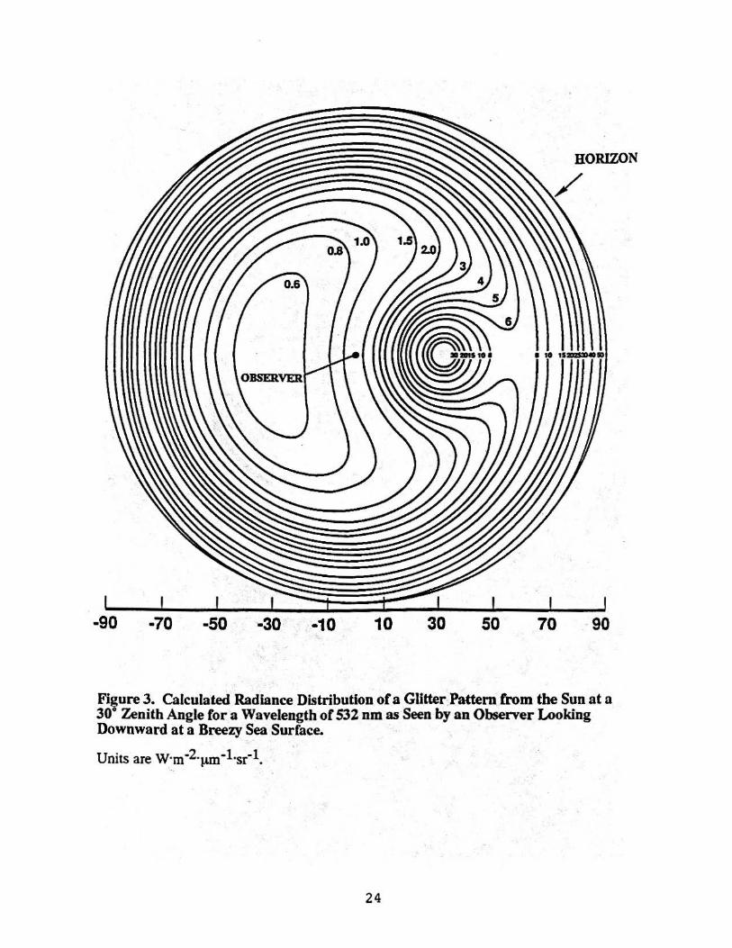
Results of modeling the sun-sky background radiance and "bouncing" it off the

surface of an idealized ocean by use of Fresnel's reflection equations are illustrated in

figure 3, which shows the angular distribution of power for an arbitrary sun zenith angle

of 30° and a wavelength of 0.5 µm. For the MWIR band and, even more so, for the

LWIR band, the magnitudes of the upwelling radiance will be considerably less than at

0.5 µm although the spatial distributions will be similar.

It is proposed to model sun glitter only in the MWIR band by extending the data of Cox

and Munk4 to that band.

LAND TARGET AND LAND BACKGROUND MODELS

DISCUSSION

An extensive body of information exists on thermal modeling of land targets. In

general, the target is represented by an assembly of polygonal graybody radiating facets

and the effective temperature of each is calculated by considering the heating effects of

radiation from the sun, sky and terrain, radiative and convective losses to the surround,

and internal heating effects from the consumption of fuel. Heat absorbed during the day

is lost at night. The process depends on the thermal heat capacities of the structures

constituting the target, and atmospheric conditions such as the degree of overcast and the

air temperature. When the humidity is high, the sky is cloud covered, and the air

temperature is nearly constant, the scene tends not to vary much from day to night. On

the other hand when the weather is clear and cloudless both day and night, large

excursions in temperature occur. The effect of a strong wind is to reduce the temperature

excursions within the scene and the thermal signature is, in part, "blown away." During

and after periods of rainfall the scene tends to become more uniform in temperature and

thermal contrasts become "washed out." However, for targets that contain heat sources,

background washout may actually be advantageous in reducing the intensity of

competing features.

7

The diurnal variation in effective temperatures of background features may

exceed the variations in the targets. For example, an unexercised target of large thermal

mass parked on dark, loose, dry sand may vary little in temperature throughout a 24-hour

period while the sand temperature varies over many tens of degrees.

MODELING APPROACH

The foregoing discussion serves to illustrate the number and diversity of

parameters that must be involved in modeling of land targets and land backgrounds.

Fortunately, there already exists a significant body of information and experience

acquired by the Army which should be adaptable to Navy and Marine Corps applications.

Army agencies performing such work include the Tank-Automotive Command, the

Center for Night Vision and Electro-Optics and the Ballistics Research Laboratory. To

avoid duplication of effort, computer programs will be acquired from such organizations

and modified as required.

AIRCRAFf TARGETS AND BACKGROUNDS

DISCUSSION

Under tri-service sponsorship, Photon Research Associates, Inc. (PRA) has

developed three complementary computer codes for modeling infrared scenes associated

with aircraft. The Target Signature Simulation (TARSIS) softwares provides a first

principles method of calculating energy emitted by and reflected from the air vehicle's

frame, but does not include plume energy. The simulation requires four inputs: (1)

atmospheric description, i.e., attenuation, path radiance, sunshine, earthshine, and

skyshine in the vicinity of the target (provided by the APART code), (2) target

description, i.e., a facet model for the target vehicle, the temperature of each facet and the

paint scheme, (3) sensor description, i.e., spectral bandwidth and response, field of view

and resolution, and ( 4) viewer geometry, i.e., positions of the target, sun and observer.

Based on these inputs and on internal data bases describing the paint reflectances,

TARSIS calculates the source, apparent, and target/background contrast intensities.

These intensities or signatures are available spatially (i.e., for each facet) and spectrally

(i.e., as a function of wavelength) and as a function of radiation source. The software has

8

been designed for rapidly generating sequences of these signatures as range and aspect

are varied.

The other two PRA codes are GENESSIS and APART. GENESSIS is used for

modeling the background and APART, which is based on LOWTRAN, is used for

performing the atmospheric calculations.

MODELING APPROACH

The TARSIS software is written in ANSI-standard FORTRAN 77. Copies of the

code and documentation are available through the Naval Ocean Systems Center.

ATMOSPHERIC TRANSMISSION MODELING

OVERVIEW

One of the most crucial issues affecting the accurate prediction of the

performance of an infrared imaging device is the modeling of the transmission of infrared

radiation through the atmosphere. While modeling of targets and backgrounds may, to a

large extent, be concerned with how realistic their simulated images appear, modeling of

the atmosphere may govern whether their images appear at all. This issue is of great

importance in deciding what infrared band should be selected for a particular application;

considerable sums of money could be wasted by a misguided choice.

Attenuation occurs in the atmosphere by absorption and by scattering of radiation.

Absorption takes place because certain molecules in the atmosphere (e.g., C00 H10,

03) possess electric or magnetic dipole moments which serve as "handles" by which an

electromagnetic field can "seize" the molecules and impart to them energy of vibration or

rotation at certain allowable frequencies, resulting in a reduction in the energy of the field

at those frequencies. At very low pressures, such absorption occurs over very narrow

frequency intervals. However, at higher pressures (e.g., atmospheric pressure), because

of increased interaction of the molecules at shorter distances and shorter mean times

between collisions, this frequency interval broadens and, as a result, the wings of the

absorption lines overlap and, depending on the particular constituent, may form a broad

band continuum in addition to the fundamental absorption lines. Water vapor, the most

9

important and the most variable atmospheric molecular absorber in the infrared; exhibits

continuum absorption in addition to spectral line absorption.

Attenuation by scattering results from radiation being redirected from its normal

path by particles in the atmosphere and therefore not intercepted by the sensor. The most

important scatterers are those particles whose dimensions are larger than or comparable

to the wavelength of the radiation. For the infrared bands, aerosols, consisting mostly of

water droplets suspended in the air in the form of haze or fog, are the important

scatterers. In general, there is a wide distribution of particle sizes within a given haze or

fog; furthermore, the shape of the distribution depends upon the type of atmosphere (e.g.,

maritime, urban, rural, desert). One measure of the aerosol content in the atmosphere is

the "daylight visibility range" (often called meteorological range or simply "visibility").

Visibility is defined as the horizontal distance over which the apparent contrast in

daylight between two large objects exhibiting 100% contrast is reduced to 2%. Although

visibility is defined only for the visible part of the spectrum, it is often extended into the

infrared by use of scaling rules that take into account wavelength and the distribution of

particle sizes, the latter usually expressed in terms of the type of atmosphere (maritime,

rural, etc.).

ATMOSPHERIC TRANSMISSION MODELS

Absorption of infrared radiation by atmospheric gases has been studied

extensively under both control.led laboratory conditions and in the real atmosphere. The

Infrared Handbook6 cites 114 references on the subject and lists an additional 197

publications in a bibliography. Various establishments, notably the Air Force

Geophysics Laboratory (AFGL), have sought to filter, purify and distill this enormous

body of corporate knowledge in the form of computer codes. AFGL has published

models and computer codes that permit calculation of transmission at high spectral

resolution (FASCOD2), moderate resolution (MODTRAN) and low resolution

(LOWTRAN). In addition, AFGL has prepared HITRAN, which is not a transmission

model, but a data base of molecular spectroscopic parameters. Other models in current

use are the Photon Research Associates, Inc. Atmospheric Propagation and Radiative

Transfer (APART) computer code. The model in most common use is LOWTRAN 7,

whose resolution is adequate for modeling thermal imaging devices.

10

LOWTRAN has been available in its various embodiments for almost twenty

years. During that time it has often been criticized for not being perfect and consequently

many revisions and improvements have been made. It is generally acknowledged that for

moderate water vapor concentrations and moderate path lengths, LOWTRAN works

quite well. However, there have been anecdotal reports that LOWTRAN seriously

underpredicts performance in the LWIR band particularly for long paths containing large

amounts of water vapor. For example, there have been reports of the detection of ships in

the Indian Ocean by fleet airborne FLIRs at ranges of the order of 50 to 70 nmi.

Unfortunately, quantitative environmental data adequate to permit calculation of

expected detection ranges were lacking for the occasion. However, synoptic

environmental data used in the then-current version of LOWTRAN indicated a very low

probability for detection at such long ranges.

Numerous papers have been published in which LOWTRAN predictions are

compared with measured data; however, most of the measured data have been obtained

. under laboratory conditions with artificial atmospheres and no aerosols present. Data

measured over long paths (i.e., over several tens of miles) are quite limited.

In a classic series of experiments, Taylor and Yates 7,8,9 of the Naval Research

Laboratory measured atmospheric transmission in the infrared along low-altitude,

horizontal paths over Chesapeake Bay ranging in length from 305 m (1000 ft) to 16.25 ·

km (8.8 nmi) and along a nearly horizontal path of length 27.7 km (14.9 nmi) at an

average altitude of about 10,000 ft between two mountains on the island of Hawaii.

As an adjunct to the evaluation of infrared imaging equipment developed under

the Long Focal Length Imaging Demonstration (LFLID) project, Hess et at.10 engaged

Avco Everett Research Laboratory and OptiMetrics, Inc. to make direct measurements of

atmospheric spectral transmittance over a 66.2-km slant path between sites on the islands

of Maui and Lanai. Vertical profiles of air temperature and water vapor concentration

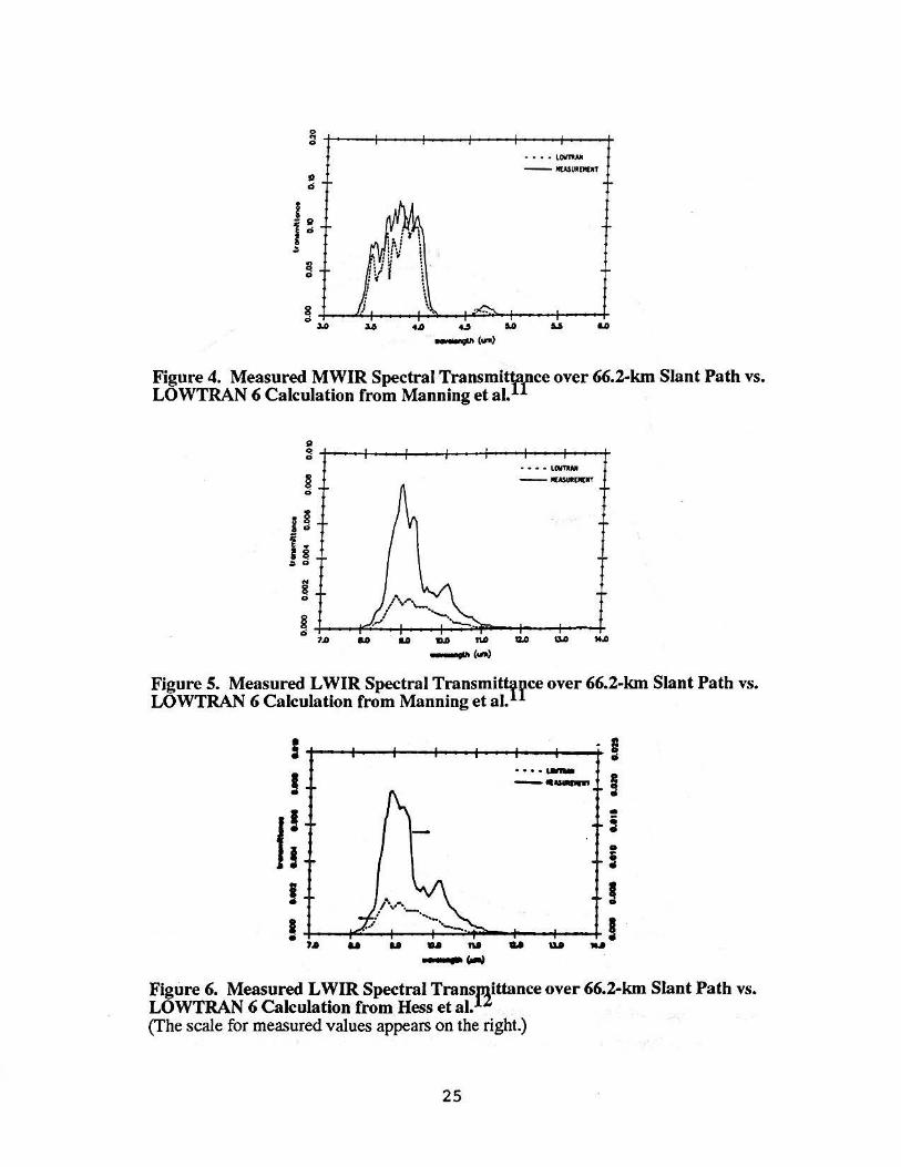
were derived from radiosonde measurements. Manning, Dowling and Hummel 11

subsequently reported that, although good agreement existed between measured data and

LOWTRAN 6 calculations for the MWIR band, LOWTRAN 6 appeared to underpredict

LWIR transmittances by factors ranging from about 2 to 4. See figures 4 and 5. After

the draft report of Manning et al.11 had been issued, it appeared that errors had been

made in presenting the measured transmittance data, the correction of which made the

11

disagreement even worse. Hess et al.12 reported the corrected data, reproduced here as

figure 6, which shows that LOWfRAN 6 is pessimistic by as much as a factor of 10.

Resolution of this issue, or at least detennining the ranges of parameters over

which LOWfRAN is valid, is of special interest in this study. Because of the

aforementioned concerns about LOWfRAN, in the Phase I proposal for this project it

was proposed that for atmospheric transmission paths containing up to 30 cm of

precipitable water, the now-current LOWfRAN 7 model would be used and for paths

containing more than 30 cm of precipitable water, the Altshulerl3 model would be used.

The Altshuler model has been applied .in the past14 with apparent success for total

amounts of water vapor in the target-to-sensor path of up to 100 cm of precipitable water.

The initial approach taken in this study was to compare predictions of

LOWfRAN 7 with those obtainable with the Altshuler model to identify potential

problems in seamlessly linking the two models. Next, comparisons were made between

LOWI'RAN 7 and the classic long-path measurements of Taylor and Yates 7,9, and

lastly, with the more recent data of Manning et at.11 and Hess et ai.12

In the Altshuler model it is assumed that transmission through water vapor can be

calculated by use of a single parameter, namely, the total amount of precipitable water

vapor in the path. This assumption greatly simplifies performance modeling of infrared

sensors. On the other hand, for LOWI'RAN 7, attenuation by water vapor depends not

only on the total amount of water vapor in the path but also on the concentration of water

vapor in the path. In the Altshuler model it doesn't matter, for example, if one has a 10-

nmi path containing 2 cm of precipitable water per nmi or a 5-nmi path containing 4 cm

of precipitable water per nautical mile. For LOWfRAN 7 the same is true of the

attenuation by the water vapor absorption lines but not for the water vapor continuum

absorption.

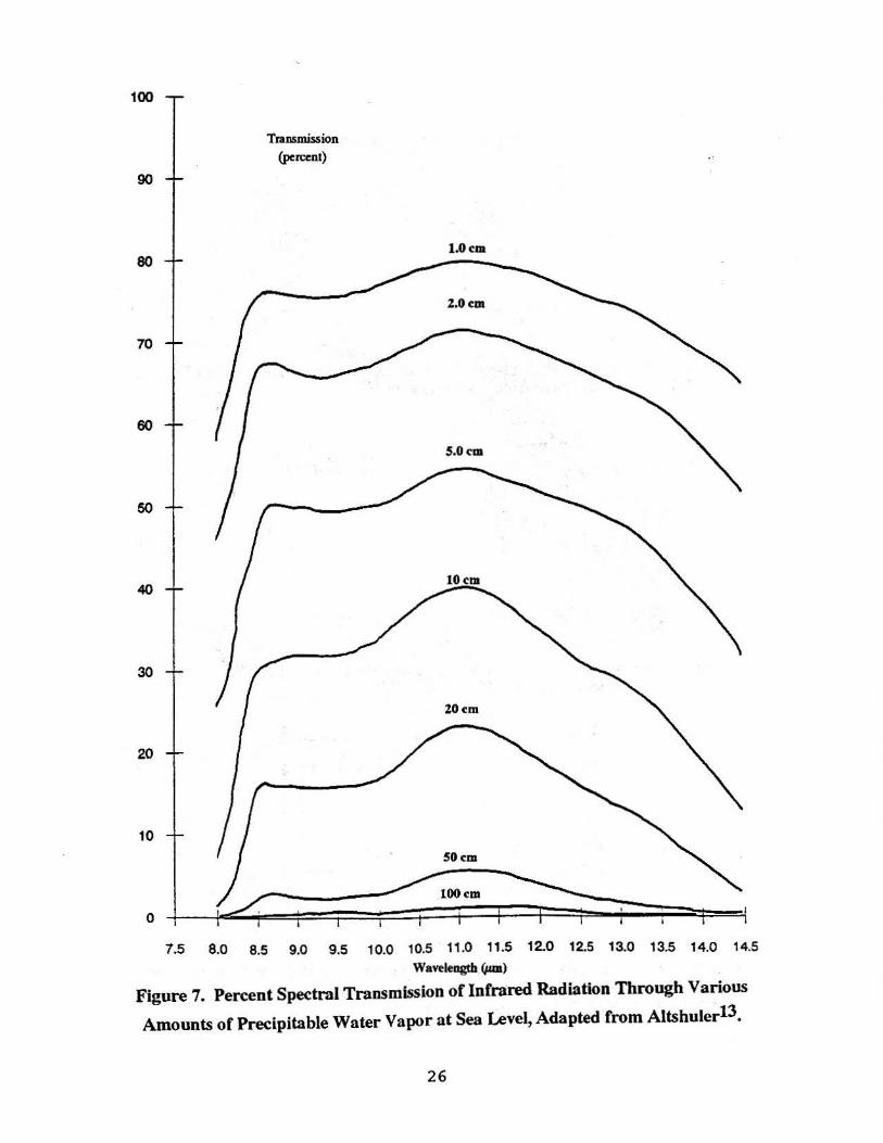
An attempt was made to see if agreement could be obtained between the Altshuler

and LOWfRAN 7 models for some reasonable range of amounts of water vapor. Figure

7 shows the spectral transmittance through total amounts of water vapor ranging from 1

to 100 cm of precipitable water obtained by following Altshuler's procedure.

LOWTRAN 7 was then nonnalized to the Altshuler model for the case of 100 cm of

precipitable water in the path. It was found that a water vapor concentration of 4.1 g/m 3

placed LOWfRAN 7 in agreement with Altshuler for the 100 cm case as shown in

12

figure 8. Note that, as was to be expected, there is reasonable agreement between the two

models for large amounts of water vapor in the path; however, for the smaller amounts,

LOWfRAN 7 predicts higher transmittances than Altshuler.

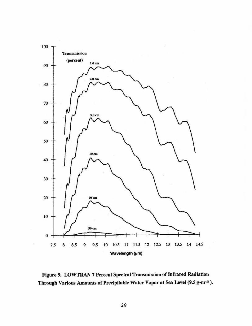
In a second example, a water vapor concentration of 9.5 g/m3 was assigned to

LOWfRAN 7 and path lengths were selected to yield the same set of total water vapor

amounts as before. The results of this trial are shown in figure 9. LOWfRAN predicts

higher transmittances for the cases corresponding to less than 10 cm of precipitable water

vapor in the path and lower transmittances for paths containing more than 10 cm of

water. Additional discrepancies exist in the peak transmission wavelength. LOWfRAN

predicts the peak transmission to occur at 9.5 µm compared to Altshuler's 11 µm.

Although it is believed that, if necessary, LOWI'RAN 7 could be made to emulate the

Altshuler model adequately (for thermal imaging purposes) over limited ranges of the

parameters, it has now been concluded that this is not the best of the available

approaches.

As part of this Phase I SBIR program a comprehensive review of computer-based

atmospheric modeling was performed. The most widely accepted standard for low

resolution atmospheric propagation models is LOWfRAN 7. This propagation model

and computer code enables the calculation of atmospheric transmittance and background

radiance from 0 to 50,000 cm·l at a resolution of 20 cm·l. Among other things, it

includes new molecular band model parameters that yield higher transmittances in the

LWIR band compared with LOWI'RAN 6. LOWTRAN 7 provides a useful starting

point for atmospheric modeling for this project. However, a potential problem area exists

in the LWIR band for moderate to high water vapor concentrations. A continuing

investigation will be required to resolve perceived .discrepancies betWeen measured data

and LOWfRAN 7 before it is implemented in the image train model. It appears at

present that the errors may be in the measured data.

The LOWTRAN models have relied heavily on a long history of measurements

by Burch and his associatesl5,16. Grant17 has provided an excellent critical review of

the state of knowledge of transmission of 8- to 13-µm radiation through water vapor.

Grant points out that the earlier work of Burch et al., which was the basis for the

attenuation coefficients associated with the water vapor continuum absorption used in

LOWfRAN 6, suffered from several sources of experimental error. In the earlier work

of Burch et al. water vapor apparently had condensed on the surfaces of the mirrors used

13

in the multiple path absorption cell for the cases of high water vapor concentration. In

Burch's more recent measurements, the mirrors were heated to prevent condensation,

which resulted in a 20% reduction in the measured coefficients. Also, earlier laboratory

measurements of absorption by water vapor were performed with nitrogen as the host gas

in the absorption ·cell. It has been found that nitrogen produces a greater broadening of

the water vapor absorption lines and, consequently, greater continuum absorption, than if

a mixture of oxygen and nitrogen corresponding to the atmosphere is used. The more

recent results form the basis for the values used in HITRAN, FASCOD2 and

LOWfRAN7.

In an attempt to determine the degree of agreement between LOWTRAN 7 and

data measured over long atmospheric paths, PSR has taken the published data of Taylor

and Yates 7,9, Manning et at.11 and Hess et a1.12 ·and computed LOWTRAN 7

transmission spectra for the MWIR and L WIR bands, using the environmental data they

provided.

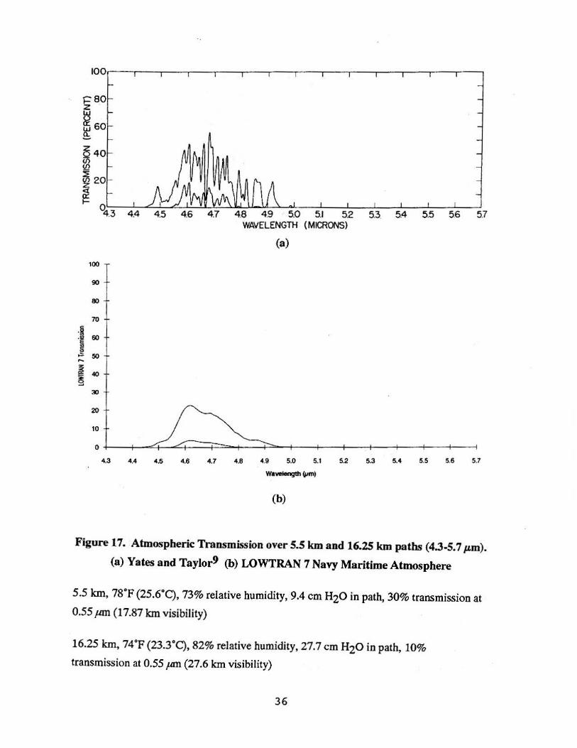
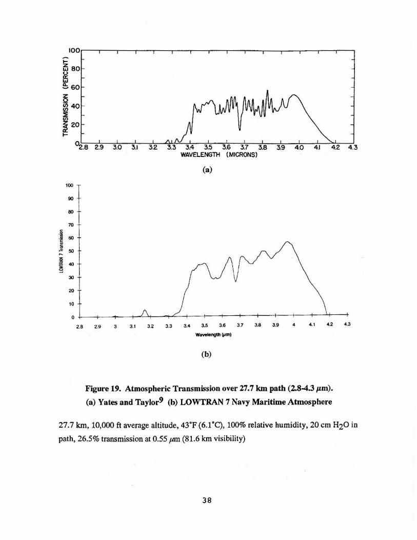
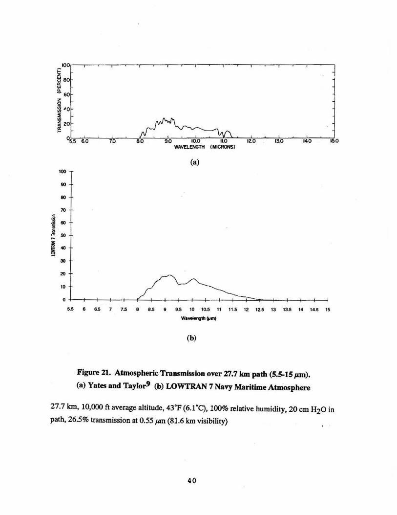
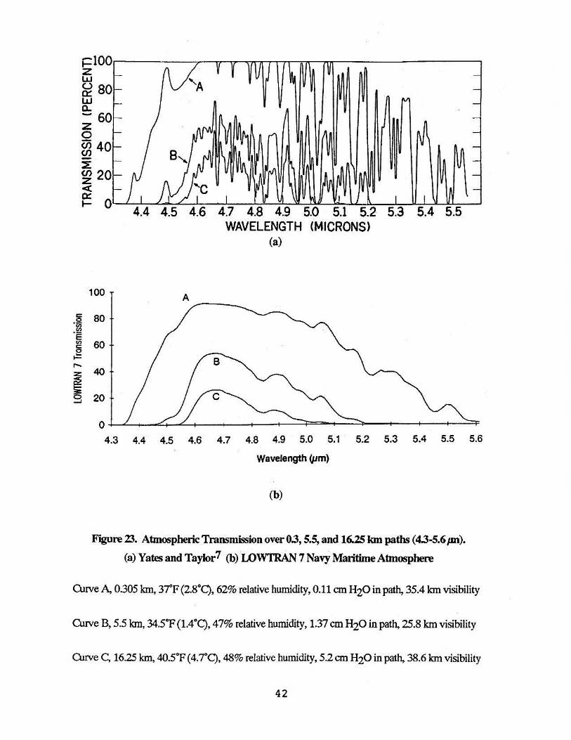
Figures 10 through 24 allow comparisons to be made between LOWI'RAN 7

results and the experimental data of Yates and Taylor. It is seen that, in most cases,

LOWfRAN 7 predicts smaller transmittances, in both the MWIR and LWIR bands, than

the values measured by Yates and Taylor. Contrary to previous expectations, there is

relatively good agreement for the longer paths of 16.25 km and 27.7 km, especially for

the cases of high visibility. For the cases of lower visibility, the disagreements become

greater, particularly for the LWIR band where LOWTRAN 7 appears to underpredict by

a factor of 2 to 3. One possible reason for the discrepancy is the way that the effects of

, visibility are scaled from the visible part of the spectrum to the infrared. If the principal

reason for poor visibility on a given occasion is a large concentration of aerosols having

particle sizes of the order of the wavelength of visible light (e.g., 0.55 µm) but a very

small concentration of particles in the size regime of about 10 µm, LOWTRAN 7 could

seriously underestimate LWIR transmittances. Kneizys et at.18 conclude, on the basis of

measurements made over 8-km and 2.25-km paths at Wright-Patterson Air Force Base,

the data showed good agreement with LOWTRAN 6 calculations, provided the

calculations were made under the assumption of no aerosols present for measurements

made under conditions of low visibility.

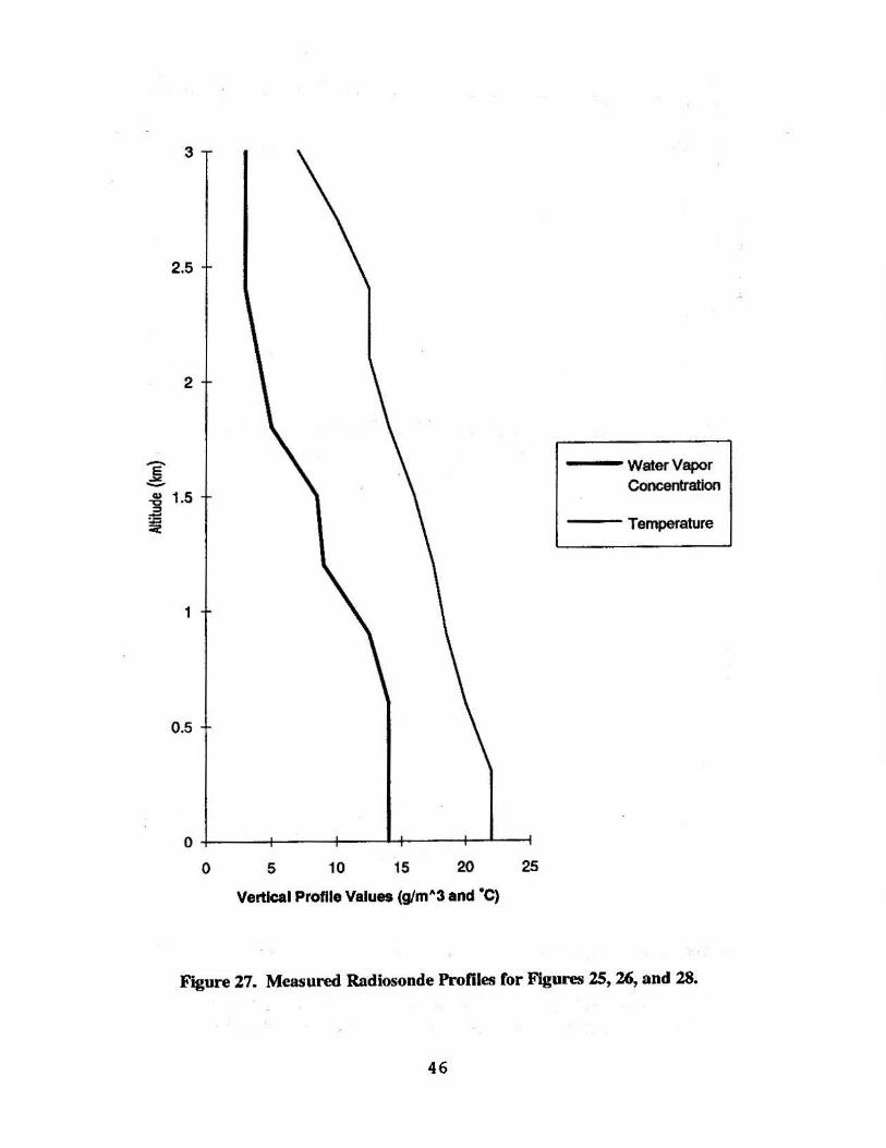
Figures 25 and 26 permit comparison of a small portion of the measured data of

Manning et al.11 with LOWTRAN 6 and LOWTRAN 7 calculations. Figure 27 shows

14

the vertical profiles of temperature and water vapor concentration in the vicinity around

the time of the transmission measurements. The absolute humidity varied from 3 to 14

grams per cubic meter as a function of altitude. Manning et al. show good agreement

between LOWfRAN 6 calculations and measured data in the MWIR band but an

underprediction by a factor of about 4 for the LWIR band. On the other hand, PSR

calculations with LOWTRAN 7, shown also in figures 25 and 26, show good agreement

with the measurements in both the MWIR and LWIR bands. Condray19 has performed a

study of LOWfRAN 6 vs. LOWfRAN 7 and concludes that, for high water vapor

concentrations, LOWfRAN 6 is more pessimistic than LOWTRAN 7, but for an absolute

humidity of 10 g/m3, the difference is only several percent. It is suspected that Manning

et al. erred in their LOWTRAN calculations.

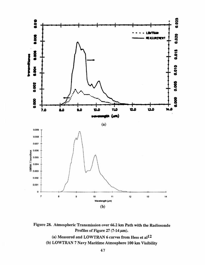
Hess et aJ.12 have presented a small subset of the Manning et al. data after

making a "correction" in the measured transmittance data, increasing those values by a

factor of 2.5. This increases the discrepancy to a factor of 10 between the measured

values and the LOWTRAN 6 values of Manning et al. Figure 28 is a reproduction of

data from Hess et al. and the PSR LOWTRAN 7 calc.ulations for the same set of

conditions.

CONCLUSIONS

A wealth of information exists in the form of documents and computer codes that

is relevant to generating synthetic infrared imagery that is, within limits, qualitatively and

quantitatively correct. Models covering both the spatial and thermal characteristics of

land, sea and air targets have been subjects of intensive development. It appears that the

greatest deficiencies occur in modeling extremely variable target backgrounds and

environmental conditions. That is, once a particular target type has been established as

being of interest, it is a relatively straightforward, although by no means trivial, task to

generate a thermal model of it. On the other hand, backgrounds and environmental

conditions can exhibit essentially infinite variability.

It appears, from the bibliographic material provided in this report, that from the

viewpoint of scene generation, relatively little work has been done in the areas of

modeling sea and sky backgrounds. Most of the reference material in these areas consists

of basic scientific papers that will have to be applied to models.

15

It is concluded that, in the area of atmospheric transmission modeling,

LOWTRAN 7, with certain qualifications, is the model of choice. It has been

recommended20 that LOWTRAN 7 be used in the modeling calculations but that

FASCOD2 also be used for occasional sanity checks to provide correction factors for

those cases in which the results from LOWTRAN 7 are questionable. Studies of the

sensitivity of results to be obtained from the infrared scene generator to errors in

atmospheric transmission calculations should be performed. For example, greater

percentage errors could be tolerated over short clear paths (for which atmospheric

attenuation is not a significant issue) than over long paths for which the atmosphere could

determine whether a target can be detected outside of its defensive envelope.

As shown in this report, LOWTRAN 7 does an amazingly good job of

"predicting" measured data. However, for certain situations (e.g., low visibility),

departures by a factor of two to three were observed. The interim solution used by some

workers has been to delete the effects of aerosol attenuation in their L WIR calculations to

obtain a better match. The conclusion is that LOWTRAN 7 should be \lSed, but used

with caution.

At the beginning of the Phase II work, a set of gUidelines should be established

restricting the range of atmospheric conditions under which LOWTRAN 7 should be

exercised in the scene generator to those for which its errors cause negligible effects.

This will allow the atmospheric model to be used, for example, in comparing

performance in the MWIR and LWIR bands. In Phase II, a rigorous investigation and

oomparison of published experimental results and LOWTRAN 7 calculations should be

performed. The previously established bounds of atmospheric water vapor and aerosol

conditions will be extended and the final recommendations for the atmospheric portion of

the image train model will be reported.· The studies will include consideration of both the

MWIR and LWIR bands to ensure that transmission in both bands is modeled correctly

and that comparisons of performance of the two bands are valid. These efforts will be

performed in parallel with other parts of the project.

16

REFERENCES

1. D. M. Wilson, "A Method of Computing Ship Contrast Temperatures Including

Results Based on Weather Ship J Environment Data," Naval Surface Weapons Center

Report NSWC/WOL TR 78-187, 29 Jan 1991

2. E. 0. Hulburt, "The Polarization of Light at Sea," Journal of the Optical Society of

America 24, 35 (1934)

3. P. M. Saunders, "Radiance of Sea and Sky in the Infrared Window 800-1200 cm·1,"

Journal of the Optical Society of America" 58, 645, (1968)

4. C. Cox and W. Munk, "Statistics of the Sea Surface Derived from Sun Glitter,"

Journal of Marine Research 16, 198 (1954)

5. Photon Research Associates, Inc. TARSIS Computer Code (Version 7.1) Reference

Manual, November 1987

6. W. L. Wolfe and G. J. Zissis, Editors, The Infrared Handbook, Environmental

Research Institute of Michigan (1985)

7. J. H. Taylor and H. W. Yates, "Atmospheric Transmission in the Infrared," Naval

Research Laboratory Report 4759, July 2, 1956

8. H. W. Yates, "The Absorption Spectrum from 0.5 to 25 Microns of a 1000-ft

Atmospheric Path at Sea Level," Naval Research Laboratory Report 5033, September 27,

1957

9. H. W. Yates and J. H. Taylor, "Infrared Transmission of the Atmosphere," Naval

Research Laboratory Report 5453, June 8, 1960

10. M. R. Hess, W. K. Hull and M. D. Gibbons, "Long Focal Length Imaging

Demonstration (U)," Proceedings of the IRIS Specialty Group on Infrared Imaging,

January 1984

17

11. J. L. Manning, J. A. Dowling and J. R. Hummel, "Ship-to-Ship Propagation:

Maritime Data Analyses," OptiMetrics, Inc. Draft Report OMI-116, December 1984

12. M. R. Hess, J. Gibbons, J. Toner, W. Abrams, R. Chin, M. Gibbons and M. Winn

"The Long Focal Length Imaging Demonstration (LFLID) Project (U)," Proceedings of

the Meeting of the IRIS Specialty Group on Infrared Imaging, March 1985

13. T. L. Altshuler," A Procedure for Calculation of Atmospheric Transmission of

Infrared," General Electric Advanced Electronics Center at Cornell University Report

R57ELC15, 1 May 1957

14. P. M. Moser, "Mathematical Model of FUR Performance," Naval Air Development

Center Tech Memo NADC-20203:PMM, AD-A045 247, 19 October 1972

15. D. A. Gryvnak and D. E. Burch, "Infrared Absorption by C02 and H20," Air Force

Cambridge Research Laboratories Report AFG~ TR-0154, AD-A060 079, May 1978

16. D. E. Burch and R. L. Alt, "Continuum Absorption by H2o in the 700-1200 cm·l

and 2400-2800 cm·1 Windows," Air Force Geophysics Laboratory Report AFGL-TR-

0128, AD-A147 391, May 1984

17. W. B. Grant, "Water vapor absorption coefficients in the 8-13-µm spectral region: a

critical review," Applied Optics 29, 451 (1990)

18. F. X. Kneizys, R.R. Gruenzel, W. C. Martin, M. J. Schuwerk, W. 0. Gallery, W. 0.

Clough, J. H. Chetwynd, and E. P. Shettle, "Comparison of 8 to 12 Micrometer and 3 to 5

Micrometer CVF Transmissometer Data With LOWTRAN Calculations," Air Force

Geophysics Laboratory Report AFG~TR-84-0171, AD-A154 219, 26 June 1984

19. P. M. Condray," A LOWfRAN7 Sensitivity Study in the 8-12 and 3-5 Micron

Bands--lncludes Comparisons with LOWfRAN6 Results," USAF Environmental

Technical Applications Center Report USAFETAC/fN-90/002, AD-A222 094, February

1990

20. M. E. Thomas, personal communication

18

BIBLIOGRAPHY

P. P. Ostrowski and D. M. Wilson, "A Simplified Computer Code for Predicting Ship

Infrared Signatures," Naval Surface Weapons Cente.r Report NSWC/fR-84-540,

AD-B099 632L, 13November1985

M.A. Mazzer, R. J. Mitchell, et al., "Computer Simulation of Warships in the Infrared

(U)," Proceedings ofIRIS 26, No. l, 209, June 1982 "· ,

P. E. Batley, "Ship Infrared Signatures (SIRS) Computer Model -Technical Overview

and User's Manual," Naval Ship Research and Development Center Report SME-78-37

(1978)

R. J. Becherer and G. L. Harvey, "Simplified Models of Ship Infrared Signatures (U),"

Proceedings of IRIS 24, 141, October 1979

D. M. Wilson and B. S. Katz, "Performance of Electro-Optics Systems Against Time

Varying Ship Signatures (U)," Proceedings of IRIS 25, No. 3, 229, March 1981

G. L. Harvey and R. J. Becherer, "Dynamic Variations of Ship Infrared Signatures,"

Naval Research Laboratory Report No. EOTP0-51, AD-C019 271L, 17 August 1979

D. Friedman, "Ship Infrared Signature (U)," Naval Research Laboratory Report 7330,

AD-518 232L, 15 October 1971

Z. C. Bennett, C. F. Bieber, et al., "The Infrared Radiant Intensity of the USS Gyatt (U),"

Naval Research Laboratory Report 6978, AD-505 766L, 15October1969

D. C. Burdick, K. D. Ervin, et al., "Interim Assessment of Ships by ltlfrared (U)," Naval

Research Laboratory Memorandum Report 1879, AD-391152L, 1May1969

H. Shenker et al., "Ship Infrared Signatures and Countermeasures (U)," Proceedings of

IRIS 15, No. 2, 225, September 1970

I. Wilf and Y. Manor, "Simulation of sea surface images in the infrared," Applied Optics,

2.1, 3174 (1984)

19

F. Rosell and G. Harvey, Editors, "The Fundamentals of Thermal Imaging Systems,"

Naval Research Laboratory Report 8311, 10 May 1979

R. D. Chapman and G. B. Irani, "Errors in estimating slope spectra from wave images,"

Applied Optics 20, 3645 (1981)

P. M. Saunders, ·"Shadowing on the Ocean and the Existence of the Horizon," Journal of

Geophysical Research 72, 4643, (1967)

N. Ben-Yosef, B. Rahat, and G. Feigin, "Simulation of IR images of natural

backgrounds," Applied Optics 22, 190 (1983)

0. E. Toler and D. S. Grey, "Simulation model for infrared imaging systems," SPIE 226

Infrared Imaging Systems Technology, 121 (1980)

T. J. Rogne, C. S. Hall, R. Freeling, G. R. Gerhart and D. J. Thomas, "U.S. Anny Tank

Automotive Command (TACOM) Thermal Image Model (TIIM)," SPIE lllOimaging

Infrared: Scene Simulation, Modeling, and Real Image Tracking, 210 (1989)

U. Bernstein, A. Stenger, and B. Kaye, "An IR imaging simulation system," SPIE 1157

Infrared Technology XV, 200 (1989)

N. Ben-Yosef, K. Wilner and M. Abitbol, "Natural terrain in the infrared: Measurements

and Modeling," SPIE 819 Infrared Technology XIII, 66 (1987)

R. I. Koda, U. Bernstein and C. E. Todd, "Generic infrared system model with dynamic

image generation," SPIE 1110 Imaging Infrared: Scene simulation, Modeling, and Real

Image Tracking, 232 (1989)

C. E. Keller, A. J. Stenger and U. Bernstein, "Improved IR image generator for real-time

scene simulation," Technology Service Corporation

U. Bernstein and C. E. Keller, "A thermal model for real-time textured IR background

simulation," SPIE International Symposium on Optical Engineering and Photonics in

Aerospace Sensing," 1-5 April 1991

20

A. T. Zavodny and M.A. Mazzer, "Simulation of cultural scenes for passive infrared

sensors," Technology Service Corporation

S. Jandrall, E. Schweitzer and J. Barrilleaux, "A Tactical Infrared Scene Generator,"

SPIE 1110 Imaging Infrared: Scene Simulation, Modeling, and Real Image Tracking, 2

(1989)

R. J. Evans and P. M. Crane, "Dynamic FLIR simulation in flight training research,"

SPIE 1110 Imaging Infrared: Scene Simulation, Modeling, and Real Image Tracking, 11

(1989)

M. E. Thomas, "Infrared- and Millimeter-Wavelength Continuum Absorption in the

Atmospheric Windows: Measurements and Models," Infrared Physics, 30, 161, (1990)

C. T. Delaye and M. E. Thomas, 11 Atmospheric continuum absorption models," SPIE

Vol. 1487 Propagation Engineering: Fourth in a Series ( 1991)

S. A. Clough, F. X. Kneizys, R. Davies, R. Gamache and R. Tipping, "Theoretical Line

Shape for H20 Vapor; Application to the Continuum," Atmospheric Water Vapor, A.

Deepak, T. D. Wilkerson and L. H. Ruhnke, Editors, Academic Press, New York (1980)

F. X. Kneizys, E. P. Shettle, W. 0. Gallery, J. H. Chetwynd, L. W. Abreu, J.E. Selby,

S. A. Clough and R. W. Fenn, "Atmospheric Transmittance/Radiance: Computer Code

LOWTRAN 6," Air Force Geophysics Laboratory Report AFGL-TR-0187, 1 August

1983

F. X. Kneizys, E. P. Shettle, L. W. Abreu, J. H. Chetwynd, G. P. Anderson,

W. 0. Gallery, J.E. Selby and S. A. Clough, "Users Guide to LOWTRAN 7," Air Force

Geophysics Laboratory Report AFGL-TR-88-0177, 16 August 1988

A. D. Devir, A. Ben-Shalom, S. G. Lipson, U. P. Oppenheim and E. Ribak, "Atmospheric

Transmittance Measurements: Comparison with LOWTRAN 6, Report RAN99-85,

Technion-Israel Institute of Technology, Haifa 32000, Israel (1985)

L. L. Smith, T. Hilgeman and B. Sandford, "Long-Path Airborne Infrared Atmospheric

Transmission (U)," Proceedings of IRIS 28, 193, June 1983

21

"' "'

Figure 1. Infrared Line Scanner Image of a Decks-Awash Submarine off Block Island Recorded in the LWIR Band

Date: 3 Aug 1970 Time: 1225Q

Only the sail structure of the submarine can be seen distinctly. Note the relative absence of sun glitter.

~ w

Figure 2. Infrared Line Scanner Image of a Decks-Awash Submarine off Block Island Recorded in the MWIR Band

Date: 3 Aug 1970 Time: 1237Q

Note that in this spectral band the sail structure of the submarine is difficult to detect because of sun glitter.

HORIZON

-90 ·70 -50 .• 30:· . ·10 10 30 50 70 90

Fi~ure 3. Calculated Radiance Distribution or a Glitter· Pattern Crom the Sun at a 30 Zenith Angle for a Wavelength of 532 nm as Seen by an Observer Looking Downward at a Breezy Sea Surface.

Units are ~·m·2.µm-l.sr·l.

24

0 0

--··lOllftM

- "USUl[M[llT

Figure 4. Measured MWIR Spectral Transmityyice over 66.2-km Slant Path vs. LOWTRAN 6 Calculation from Manning et al. .

9 ~ 0

§ 0

i ! '2 c . ~ D ..

g 0

§ 0

1.1>

Figure 5. Measured LWIR Spectral Transmittyyce over 66.2-km Slant Path vs. LOWTRAN 6 Calculation from Manning et al.

! I • !

···-~

! _ .. .....,...

1: .. 2 • 2

! ! I • , .. ... ... ... NI ... WI

1· ... ..,......_.,, Figure 6. Measured LWIR Spectral Transflittance over 66.2-km Slant Path vs. LOWTRAN 6 Calculation from Hess et al. (The scale for measured values appears on the right.)

25

100

90

80

70

60

50

40

30

20

10

0

Tn~mis.sion

(percent)

l.O~m

7.5 8.0 8.5 9.0 9.5 10.0 10.5 11.0 11.5 12.0 12.5 13.0 13.5 14.0 14.5 Wanlength (µm)

Figure 7. Percent Spectral Transmission of Infrared Radiation Through Various

Amounts of Precipitable Water Vapor at Sea Level, Adapted from Altshuler13.

26

100

90

80

70

60

50

40

30

20

10

0

Transmission

(percent) 1.0 Cl1I

7 .5 8 8.5 9 9 .5 10 10.5 11 11.5 12 12.5 13 13.5 14 14.5

Wavelength ~m)

Figure 8. LOWTRAN 7 Percent Spectral Transmission of Infrared Radiation

Through Various Amounts of Precipitable Water Vapor at Sea Level (4.1 g-m-3 ).

27

100

Transmission

(percent) 1.0 CIJI

7.5 8 . 8.5 9 9.5 10 10.5 11 11.5 12 12.5 13 13.5 14 14.5

Wavelength (I'm)

Figure 9. LOWTRAN 7 Percent Spectral Transmission of Infrared Radiation

Through Various·Amounts of Precipitable Water Vapor at Sea Level (9.5 g-m·3 ).

28

c ·~ .. ·e .. c

~ ,... ~ ~ ....

·:I 70

60

50

"° 30

20

10

0

2.8 2.9 \ 3.0 3.1

3.4 3.5 3.6 3.7 3.8 3.9 4.0 4.1 42 4.3 WAVELENGTH (MICRONS)

(a)

3.2 3.3 3.4 3.5 3.6 3.7 3.8 3.9 4.0 4.1 4.2 4.3

Wavelength ~m)

(b)

Figure 10. Atmospheric Transmission over S.5 km and 16.25 km paths (2.8-4.3 µ,m).

(a) Yates and Taylor9 (b) LOWTRAN 7 Navy Maritime Atmosphere

5.5 km, 38°F (3.3°C), 66% relative humidity, 2.2 cm H20 in path, 40% transmission at

0.55 µm (23.5 km visibility)

16.25 km, 53°F (11.7°C), 41 % relative humidity, 6.5-6.9 cm H20 in path, 29%

transmission at 0.55 µm (51.4 km visibility)

29

100 -t-z w 80 0 a:: w ~60 z 0 (()40 (/')

:::? (/') z 20 <[ a:: t-

04.3 4.4 4.5 4.6 . 4.7 4.8 4 .9 5.0 5.1 5.2 5.3 5.4 5.5 5.6 5.7 WAVELENGTH (MIC RONS)

(a)

100

90

80

70 c

.S! "' ·~ "' c 0

60

..= 50 ,...

~ 40 ~

30

20

10

0

4.3 4.4 4.5 4.6 4.7 4.8 4.9 5.0 5.1 5.2 5.3 5.4 5.5 5.6

Wavelength (pm)

(b)

Figure 11. Atmospheric Transmission over S.5 km and 16.25 km paths (4.3-S. 7 µm).




16.25 km, 53°F (11.7°C), 41 % relative humidity, 6.5·6.9 cm HzO in path, 29%


30

5.7

,__ z t5 8 a: LI.I ~60 z 0

~ 40 ~ (/)

~ 2 a:: ....

05:s s.o

100 T 90

eo

70

7.0 90 10.0 11.0 12.0 14.0 15.0

WAVE LENGT H (M ICRONS)

(a)

:1 60

~ .....

I 50

40

30

20

5.5 6.0 6.5 7.0 7.5 8.0 8.5 9.0 9.5 10.0 10.5 11.0 11 .5 12.0 12.5 13.0 13.5 14.0 14.5 15.0

Wavelength (µm)

(b)

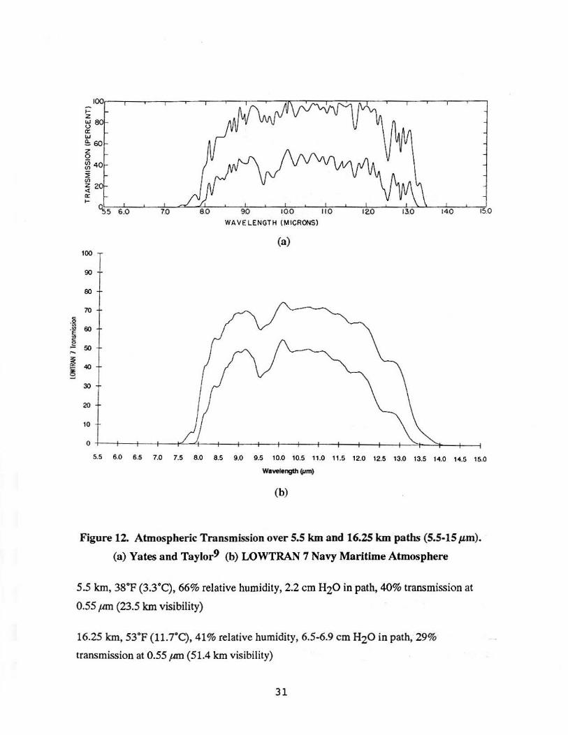
Figure 12. Atmospheric Transmission over 5.5 km and 16.25 km paths (5.5-15 µm).




16.25 km, 53°F (11.7°C), 41 % relative humidity, 6.5-6.9 cm HzO in path, 29%


31

100 ...... t-zeo w (,) a:: ~60

z ~40 (/)

~ (/) 20 z ~ 0::

t- 02.e 2.9 30 3.1 3.2 3.3 3.4 3.5 3.6 3.7 3.8 3.9 4.0 4.1 4.2 4.3 WAVELENGTH (MICRONS)

(a)

·: t ao

70 a :~ 60 E "' c ,g

50 ......

I 40

30

=t 0

2.8 2.9 3.0 3.1 3.2 3.3 3.4 3.5 3.6 3.7 3.8 3.9 4.0 4.1 4.2 4.3

Wavefength (pm)

(b)

Figure 13. Atmospheric Transmwion over S.S km and 16.25 km paths (2.8-4.3 µ,m).


5.5 km, 64°F (17.8°C), 51 % relative humidity, 4.18 cm H20 in path, 70% transmission

at 0.55 µm (60.3 km visibility)

16.25 km, 68.7°F (20.4°C), 53% relative humidity, 15.1 cm H20 in path, 43%


32

100

I-z w 80 0 a::

~ 60 _,

z Q (/) 40 (/)

~

~ 20 4 a:: I-

04.3 4 .4 4.5 4.6 4.7 4.8 4.9 5.0 5.1 5.2 5.3 5.4 5.5 5.6 . 5.7 WAVELENGTH (MICRONS)

(a)

100

90

eo

70 .. ·~ ·1 60

,g 50 ....

I 40 ~

30

20

10

0

4.3 4.4 4.5 4.6 4.7 4.8 4.9 5.0 5.1 5.2 5.3 5.4 5.5 5.6 5.7

Wavetength (I'm)

(b)

Figure 14. Atmospheric Transmission over 5.5 km and 16.25 km paths (4.3-5.7 µm).


5.5 km, 64°F (17.8°C), 51 % relative humidity, 4.18 cm H20 in path, 70% transmission


16.25 km, 68.7°F (20.4°C), 53% relative humidity, 15.1 cm HzO in path, 43%


33

" .2 "' .111 E "' "' ~ ....

~ g

>=" ~ 80 0 a: ~60

~ 40 ~ i ~ 20 <C a: ~ 01L--L~.1.---L~..J..,...1:.:L.l~-'-__.L~-'---'~-'-~"-:--_._~":-:---""-~-':-:--'-~-'-:--'-~

5.5 6 .0 70 8.0 9 .0 10.0 11 .0 12.0 13.0 140 15.0

100

90

80

70

60

so

4()

30

20

10

WAVELENGTH (MICRONS)

(a)

5.5 6.0 6.5 7.0 7.5 8.0 8.5 9.0 9.5 10.0 10.5 11.0 11 .5 12.0 12.5 13.0 13.5 14.0 14.5 15.0

W•~(flm)

(b)

Figure 15. Atmospheric Transmission over 5.5kmand16.25 km paths (5.5-15 µm) .


5.5 km, 64°F {l 7.8°C), 51 % relative humidity, 4.18 cm HzO in path, 70% transmission


16.25 km, 68.7°F (20.4°C), 53% relative humidity, 15.1 cm H20 in path, 43%


34

IOO

~ z 80 LLJ (.) a: ~60

~ 40 (/)

~ 20 ct a:: ~

02a 2.9 3.0 3.1 32 3.3 3.4 3.5 3.6 3.7 3.8 3.9 4.0 4.1 42 4.3


(a)

100

90

80

70 c:

.S! .. -~ 60

Ct ..::: 50 .....

i ...J

'I()

30

20

10

0

2.8 2.9 3.0 3.1 3.2 3.3 3.4 3.5 3.6 3.7 3.8 3.9 4.0 4.1 4.2 '4.3

Wawtength (µm)

(b)

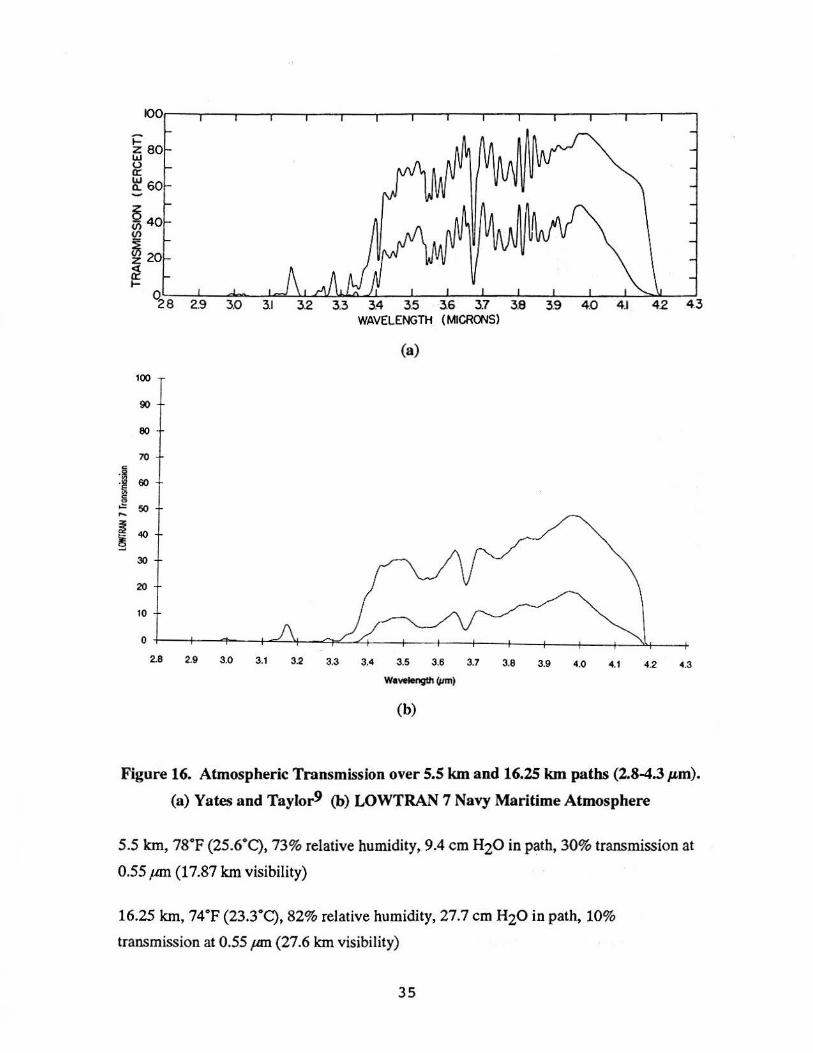
Figure 16. Atmospheric Transmission over S.S km and 16.25 km paths (2.8-4.3 µ.m).


5.5 km, 78°F (25.6°C), 73% relative humidity, 9.4 cm HzO in path, 30% transmission at


16.25 km, 74°F (23.3°C), 82% relative humidity, 27.7 cm H20 in path, 10%


35

100

i=" 80 z · w ffi 60 ~

~40 (f)

~

~ 20 <t a:: t-

04.3 4.4 4.5 4.6 4.7 4.8 4.9 5.3. 5.4 5.5 5.6 5.7 WAVELENGTH

(a)

100

90

80

70

.Ii J3 60 !ii ! 50 ....

i 40

30

20

10

0

4.3 4.4 4.5 4.6 4.7 4.8 4.9 5.0 5.1 5.2 5.3 5.4 5.5 5.6 5.7

Wawlength ~m)

(b)

Figure 17. Atmospheric Transmw ion over 5.5 km and 16.25 km paths (4.3-5. 7 µ.m).

(a) Yates and Taylor9 (b) WWTRAN 7 Navy Maritime Atmosphere



16.25 km, 74°F (23.3°C), 82% relative humidity, 27.7 cm HzO in path, 10%


36

c: .2 ., -~ c:

,'§. .....

~ ~ _,

100

90

80

70

60

50

40

30

20

10

(a)

5.5 6.0 6.5 7.0 7.5 8.0 8.5 9.0 9.5 10.0 10.5 11.0 11.5 12.0 12.5 13.0 13.5 14.0 14.5 15.0

W•velength (µm)

(b)

Figure 18. Atmospheric Transmission over 5.5 km and 16.25 km paths (S.5-15 µ.m).




16.25 km, 74°F (23.3°C), 82% relative humidity, 27.7 cm HzO in path, 10%


37

100 ...... I-

ffi 8 0 u a:: w & so

~ ~ 40

~ ~ 20 a: I-

02.s 2.9 3.0 3.1 3.2 3.4 3.5 3.6 3.7 3.8 3.9 4.0 4.1 4.2

100

90

80

70

·~ 60 ·~

c ,g 50 .... ~ ~

40

~ T

=t 0

2.8


(a)

2.9 3 3.1 3.2 3.3 3.4 3.5 3.6 3.7 3.8 3.9 4 4.1 4.2

Wavelength (I.Im)

(b)

Figure 19. Atmospheric Transmission over 27.7 km pa th (2.8-4.3 µ.m).


4 .3

4 .3

27.7 km, 10,000 ft average altit\lde, 43°F (6.1°C), 100% relative humidity, 20 cm HzO in

path, 26.5% transmission at 0.55 µm (81.6 km visibility)

38

100 .... ..... ~ 80 0 a:: w ~60

~ ~ 40

~ ~ 20 a; ....

043 4.4 4.5 4.8 4.9 5.0 5.1 5.2 5.3 5.4 5.5 5.6 WAVELENGTH (MICRONS)

(a)

100

90

80

70

-i ·~ 60 c: ~ 50 .... ~ ~ ~

30

20

10

0

4.3 4.4 4.5 4.6 4.7 4.8 4.9 s 5.1 5.2 5.3 S.4 5.5 5.6

W•velengdl IJ'm)

(b)

Figure 20. Atmospheric Transmission over 27.7 km path (4.3-5.7 µm).


5.7

5.7

27.7 km, 10,000 ft average altitude, 43°F (6. l 0 C), 100% relative humidity, 20 cm H20 in


3 9

100

90

80

70

·I eo 1 ~ ....

I 40

30

20

10

0

05L_5-6J....o--'--~1.o~-'---='(d!-__._---;9f;._o:--_.__-;,do.-no--'...__7,ln~..__.,,2.~o~_,__,,ri3_no-'--1.14tr.or-......__~~-o

5.5 8 6.5 7 7.f> 8 8.5 9

WAVELENGTH

(a)

9.5 10 10.5 11 11.5 12 12.S 13 13.S 14 14.5 15

Wawlengtfl (llm)

(b)

Figure 21. Atmospheric Transmmion over 27.7 Jan· path-(5.5-15 µm).

(a) Yates and Tayfor9 (b) LOWTRAN 7 Navy Maritime Atmosphere

27.7 km, 10,000 ft average altitude, 43°F (6.l 0C), 100% relative humidity, 20 cm HzO in


40

c: 0 ·~

"' ·e: "' c

~ ,....

I

100 A

80

60

40

20

04-...L.;--=~~......c~~~~--~----~--~-------+-~-+--"'*

2.8 2.9 3.0 3.1 3.2 3.3 3.4 3.5 3.6 3.7 3.8 3.9 4.0 4.1 4.2

Wavelength (µm)

(b)

Figure 22. Atmospheric Transmmion over 0.3, 5.5, and 16.25 km patm (2.8-4.2 p:n).


Ouve A, 0.305 km, 3/F (2.8°q, 62% relative hwnidity, 0.11 cm H20 in path, 35.4 km visibility

Onve B, 5.5 km, 34.5°F (1.4°q, 47% relative humidity, 1.37 cm H20 in path, 25.8 km visibility

Ouve C, 16.25 km, 40.5°F ( 4.7°q, 48% relative hwnidity, 5.2 cm H20 in path, 38.6 km visibility

41

i=too..--~~~~----..-...,......... ......................... """P"T""" ............. --...--~~~~~~~____, z w ~ 80 UJ 0.. - 60 z 0 ~40 -% ~ 20 <(

~ 0'--''--'--'---'--'----'-~-'-''---'"'--"'--u.&...---...~~-'---"'-'-""'-""-'----4. 4 4.5 4.6 4.7 4.8 4.9 5.0 5.1 5.2 5.3 5.4 5.5

WAVELENGTH (MICRONS> (a)

100 A

:I so E ~ 60 .g

o.!-L---...:::::.~~~---~-+-~-+---==;::==-+~~~-t-~-+-~-+--==i'

4.3 4.4· 4.5 4.6 4.7 4.8 4.9 5.0 5.1 5.2 5.3 5.4 5.5 5.6

Wavelength (µm)

(b)

Figure 23. Atmospheric TnmSm~ion over 0.3, S.S, and 16.25 Ian patm (4.3-5.6 pn).

(a) Ya~ and Taylor7 (b) WWfRAN 7 Navy Maritime Atmosphere

Curve A, 0.305 km, 37°F (28°C), 62% relative humidity, 0.11 cm HzO in path, 35.4 km visibility

Curve B, 5.S km, 34.5°F (1.4°C), 47% relative humidity, 1.37 cm H20 in path, 25.8 km visibility

Curve C, 16.25 km, 40.S°F ( 4./C), 48% relative humidity, 5.2 cm H20 in path, 38.6 km visibility

42

~100.--~~~-r.--~~~~~~~~~~~~~"T7"Cnr'll'--.;-'7\'"7r'TI

z ~80 a: w e: 60 z ~40 en

~ 20 <t: ~ O~-'-~.J-ct!.~~~-'-~--l'--~--'-~~-L..~~_.__,._~

7.0 75 8.0 85 9.0 95 10.0 11.0 12.0 130

c; .2 <n

• !!? E <n ~ 0 .=: ,....

i 0 .....J

100

80

60

40

20

0

6.5 7.0 7.5 8.0 8.5

WAVELENGTH <MICRONS>

9.0

(a)

9.5 10.0 10.5 11.0 11.5 12.0 12.5 13.0 13.5 14.0

Wavelength Ulm)

(b)

Figure 24. A~pheric Transmmion over 0.3, S.S, and 16.2.; Ian patm (6.5-14 pn).

(a) Yates and Taytor7 (b) LOWI'RAN 7 Navy Maritime Atmosphere

Curve A, 0.305 km, 3/F (2.8°C), 62% relative humidity, 0.11 cm HzO in path, 35.4 km visibility

Curve B, 5.5 km, 34S'F (1.4°C), 47% relative humidity, 137 an HzO in path, 25.8 km visibility

Curve C, 16.25 km, 40.5°F ( 4. IC), 48% relative humidity, 5.2 an HzO in~ 38.6 km visibility

43

j

0 N d .

~ 0

3.0

0.14

0.12

0.1

·~ 0.08 c 0 ,:;

..... I 0.06

0.04

0.02

0

3

3..5 4.0 4..5

""••ngtlt (an)

(a)

3.5 4 4.5

WllWlenglh ~m)

(b)

5.0

5

• • - • LCMTRAft

--- MEASUREMENT

5.5 6

Figure 25. Atmospheric Transmission over 66.2 km Pa th with the Radiosonde Profiles of Figure 27 (3-6 µm).

(a) Measured and LOWTRAN 6 curves from Manning et alll

(b) LOWTRAN 7 Navy Maritime Atmosphere 100 km Visibility

44

Q 0 0

N

~ 0

0.009

0.008

0.007

§ 0.006 0

;!;! i 0.005 ~ i 0.004

...... 0.003

0.002

0.001

0

7.0 a.o

7 8

- - • • lOWTRAN --- MEASUREMENT

9.0 10.0 11.0 14.0

wavelength (wn)

(a)

9 10 11 12 13 14

(b)

Figure 26. Atmospheric Transmission over 66.2 km Path with the Radiosonde Profiles of Figure 27 (7-14µm).

(a) Measured and LOWTRAN 6 curves from Manning et atll (b) LOWTRAN 7 Navy Maritime Atmosphere 100 km Visibility

45

3

2.5

2

]' -cu 1.5

i

1

0.5

0 +-~~-+-~~-+-~---11-f-~~-+--''---~

0 5 10 15 20 25

Vertical Profile Values (g/m"3 and ·c)

---Water Vapor Concentration

Temperature

Figure 27. Measured Radiosonde Profiles for Figures 25, 26, and 28.

46

• •

= ····~

I •&SUllNll

•

! -! i • 0 I'.-.. . .. . . -. . .. . .._ I . ' ,··· ......... , 0

1.0 u u 1l.O n.o ... .... .. (Illa)

(a) 0.009

0.008

0.007

~ 0.006 0 = ·e ll! 0.005 0

"" ,.... I 0.004

..... 0.003

0.002

0.001

0

7 8 9 10 11 12 13 14

Wavele"IJlll (I'm)

(b)

Figure 28. Atmospheric Transmission over 66.2 km Path with the Radiosonde Profiles of Figure 27 (7-14 µm).

(a) Measured and LOWTRAN 6 curves from Hess et aJ12

(b) LOWTRAN 7 Navy Maritime Atmosphere 100 km Visibility

47

e 0

~ 0

• -~ 0 -0 d

I ci

I d

Documents

MODELING OF TARGETS, BACKGROUNDS FOR SYNTHETIC GENERATION …