Embed Size (px)
Citation preview
Modeling of Thermomechanical Properties of PolymericHybrid Nanocomposites
Rohit Kothari,1 Shailesh I. Kundalwal ,1 Santosh K. Sahu,1 M.C. Ray2
1Discipline of Mechanical Engineering, Indian Institute of Technology, Indore 453552, India
2Department of Mechanical Engineering, Indian Institute of Technology, Kharagpur 721302, India
This article reports modeling of effective thermome-chanical properties of multifunctional carbon nanotube(CNT)-reinforced hybrid polymeric composites (hereaf-ter, it is referred as “fuzzy fiber composite”). The novelconstructional feature of fuzzy fiber composite (FFC) isthat nanoscale CNTs are radially grown on the circum-ferential surfaces of microscale carbon fibers. Severalmicromechanical models were developed to predictthe effective thermomechanical properties of FFC. Thewaviness of CNTs is intrinsic to many manufacturingprocesses and it influences thermomechanical behav-ior of two-phase CNT-reinforced composites. There-fore, an endeavor was also made to investigate theeffect of wavy CNTs on the effective thermomechanicalproperties of FFC. The proposed modeling approachwas applied to a heat exchanger made of FFC todetermine its effective thermal conductivities. The find-ings of our study suggest that FFC containing nano-and micro-scale fillers show improved thermomechani-cal properties and are promising next-generation poly-meric composites for advanced structural applications.POLYM. COMPOS., 00:000–000, 2017. VC 2017 Society of PlasticsEngineers
INTRODUCTION
The discovery of carbon-based nanomaterials such as
carbon nanotubes (CNTs) [1] and graphene [2] has stimu-
lated a tremendous research on the prediction of their
remarkable mechanical and thermal properties. Numerous
experimental and numerical studies revealed that Young’s
moduli of CNTs and graphene are in the terapascal range
[3–7]. CNTs and graphene sheets also exhibit remarkable
thermal properties different from other known materials
and they are promising candidates in many advanced
applications [8–12]. A CNT can be viewed as a hollow
seamless cylinder formed by rolling a graphene sheet and
it has attracted a lot of attention compared to graphene
system because of CNT’s one dimensional structure.
Moreover, the thermomechanical properties of CNTs are
function of their diameters. Therefore, the exceptional
thermomechanical properties of long CNTs led to the
opening of an emerging area of research on the develop-
ment of two-phase CNT-reinforced nanocomposites
[13–15] and their structural applications [16–19]. How-
ever, the addition of CNTs in polymer matrix does not
always results in improved effective properties of compo-
sites. Several important factors such as agglomeration,
aggregation, and waviness of CNTs, and difficulty in
manufacturing also play a significant role [20, 21]. These
difficulties can be alleviated using CNTs as secondary
reinforcements in the three-phase hybrid nanocomposites.
In this direction, extensive research was dedicated to the
introduction of CNTs as the modifiers to the conventional
composites to enhance their multifunctional properties.
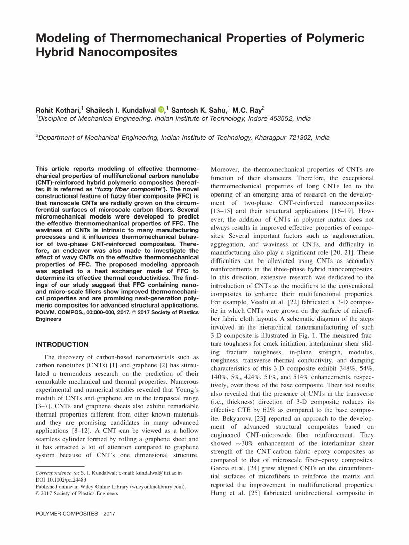
For example, Veedu et al. [22] fabricated a 3-D compos-
ite in which CNTs were grown on the surface of microfi-
ber fabric cloth layouts. A schematic diagram of the steps
involved in the hierarchical nanomanufacturing of such
3-D composite is illustrated in Fig. 1. The measured frac-
ture toughness for crack initiation, interlaminar shear slid-
ing fracture toughness, in-plane strength, modulus,
toughness, transverse thermal conductivity, and damping
characteristics of this 3-D composite exhibit 348%, 54%,
140%, 5%, 424%, 51%, and 514% enhancements, respec-
tively, over those of the base composite. Their test results
also revealed that the presence of CNTs in the transverse
(i.e., thickness) direction of 3-D composite reduces its
effective CTE by 62% as compared to the base compos-
ite. Bekyarova [23] reported an approach to the develop-
ment of advanced structural composites based on
engineered CNT-microscale fiber reinforcement. They
showed �30% enhancement of the interlaminar shear
strength of the CNT-carbon fabric–epoxy composites as
compared to that of microscale fiber–epoxy composites.
Garcia et al. [24] grew aligned CNTs on the circumferen-
tial surfaces of microfibers to reinforce the matrix and
reported the improvement in multifunctional properties.
Hung et al. [25] fabricated unidirectional composite in
Correspondence to: S. I. Kundalwal; e-mail: [email protected]
DOI 10.1002/pc.24483
Published online in Wiley Online Library (wileyonlinelibrary.com).
VC 2017 Society of Plastics Engineers
POLYMER COMPOSITES—2017
which CNTs were directly grown on the circumferential
surfaces of conventional microscale fibers. Davis et al.
[26] fabricated the carbon fiber-reinforced composite
incorporating functionalized CNTs in the epoxy matrix;
as a consequence, they observed significant improvements
in the tensile strength, stiffness, and resistance to failure
due to cyclic loadings. Zhang et al. [27] deposited CNTs
on the circumferential surfaces of electrically insulated
glass fiber surfaces. According to their fragmentation test
results, incorporation of an interphase with a small num-
ber of CNTs around the fiber remarkably improved the
interfacial shear strength of the fiber–epoxy composite.
The functionalized CNTs were incorporated by Davis
et al. [28] at the fiber/fabric–matrix interfaces of a carbon
fiber–epoxy composite. Their study showed improvements
in the tensile strength and stiffness, and resistance to ten-
sion–tension fatigue damage due to the created CNT-
reinforced region at the fiber/fabric–matrix interfaces.
Kundalwal et al. [29–31] investigated the stress transfer
characteristics of hybrid polymeric nanocomposites in
which the carbon fibers were augmented with CNTs.
Most recently, Rafiee and Ghorbanhosseini [32] devel-
oped a systematic computational modeling in the form of
hierarchical process to predict the mechanical properties
of FFC. The same authors [33] developed stochastic mul-
tiscale modeling for predicting the mechanical properties
of fuzzy fiber coated with randomly oriented CNTs.
Findings in the literature indicate that use of nanoscale
CNTs and microscale fibers together, as multiscale rein-
forcements, significantly improve the overall properties of
resulting hybrid nanocomposites, especially FFC. The
existing studies mainly focus on investigating the
enhancement of tensile strength, interfacial shear strength,
fracture toughness, and impact resistance of FFC. Surpris-
ingly, no single study was performed so far to investigate
the mechanical and thermal properties of FFC. Prediction
of effective thermomechanical properties of FFC appears
to be an important issue for further research. To establish
FFC as the superior advanced composite for structural
applications, structural analysis must be carried out and
for such analysis all effective properties of FFC must be
known a priori. Hence, this study was directed to estimate
the effective thermomechanical properties of multifunc-
tional FFC. It has been experimentally observed that
CNTs are actually curved cylindrical tubes with a rela-
tively high aspect ratio. Therefore, the effect of CNT
waviness on the effective properties of FFC was also
investigated in this study when wavy CNTs are coplanar
with either of two mutually orthogonal planes.
FUZZY FIBER NANOCOMPOSITE
The schematic diagram illustrated in Fig. 1 represents
a lamina of the FFC being investigated here. We assumed
that the wavy CNTs are uniformly spaced and radially
grown on the circumferential surfaces of microscale car-
bon fibers. Such a modified fuzzy fiber is shown in Fig.
2. Wavy CNTs are modeled as transversely isotropic solid
CNT fibers [6]. The polymer matrix is reinforced by the
fuzzy fiber and such combination can be viewed as the
representative volume element (RVE) of FFC. Such an
RVE can be considered to be made of carbon fiber
embedded in the wavy CNT-reinforced polymer matrix
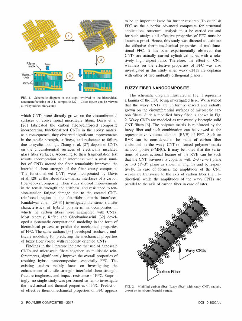
nanocomposite (PMNC). It may be noted that the varia-
tions of constructional feature of the RVE can be such
that the CNT waviness is coplanar with 2–3 (20–30) plane
or 1–3 (10–30) plane as shown in Fig. 3a and b, respec-
tively. In case of former, the amplitudes of the CNT
waves are transverse to the axis of carbon fiber (i.e., 1–
direction) while the amplitudes of the wavy CNTs are
parallel to the axis of carbon fiber in case of later.
FIG. 1. Schematic diagram of the steps involved in the hierarchical
nanomanufacturing of 3-D composite [22]. [Color figure can be viewed
at wileyonlinelibrary.com]
FIG. 2. Modified carbon fiber (fuzzy fiber) with wavy CNTs radially
grown on its circumferential surface.
2 POLYMER COMPOSITES—2017 DOI 10.1002/pc
Models of Wavy CNTs
Several earlier attempts’ have been made to investigate
the influence of wavy fibers on the effective properties
and vibrational characteristics of composites structures
[19, 35, 36]. For example, Fisher et al. [37, 38] developed
a model combining finite element results and microme-
chanical methods to determine the effective reinforcing
modulus of a wavy embedded CNT. They used a 3D
finite element model of a sinusoidal CNT embedded in
the polymer matrix to compute the dilute strain concen-
tration tensor. In another attempt, Anumandla and Gibson
[39] developed closed form micromechanics model for
estimating the effective elastic modulus of composites
containing sinusoidally wavy CNTs. Chen et al. [40]
developed an analytical curved-fiber pull-out model and
found that curved and entangled CNT greatly impacts the
thermomechanical properties of the resulting composite.
Rafiee [41] predicted Young’s modulus of polymeric
nanocomposite reinforced with nonstraight shape (sinusoi-
dal) of CNTs using multiscale modeling and demonstrated
that CNT wave considerably reduces its efficiency to
reinforce polymer matrix. As many researchers consid-
ered, we assumed sinusoidally wavy CNTs to investigate
their influence on the effective properties of FFC.
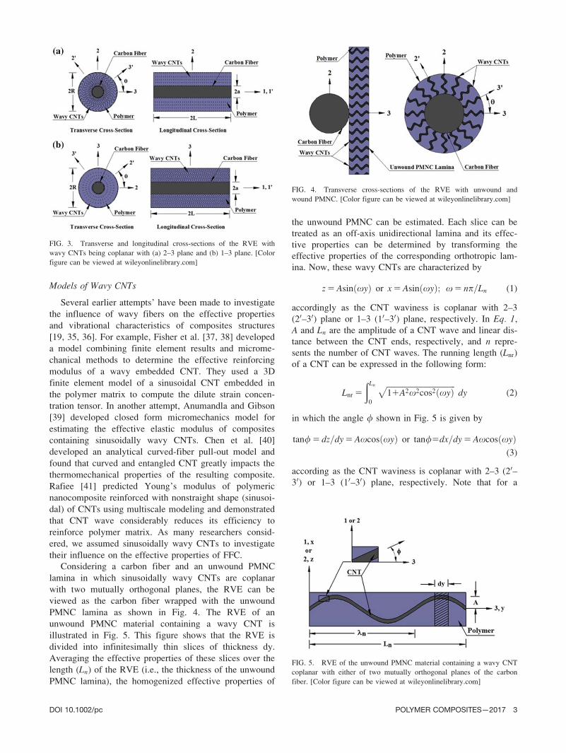
Considering a carbon fiber and an unwound PMNC
lamina in which sinusoidally wavy CNTs are coplanar
with two mutually orthogonal planes, the RVE can be
viewed as the carbon fiber wrapped with the unwound
PMNC lamina as shown in Fig. 4. The RVE of an
unwound PMNC material containing a wavy CNT is
illustrated in Fig. 5. This figure shows that the RVE is
divided into infinitesimally thin slices of thickness dy.
Averaging the effective properties of these slices over the
length (Ln) of the RVE (i.e., the thickness of the unwound
PMNC lamina), the homogenized effective properties of
the unwound PMNC can be estimated. Each slice can be
treated as an off-axis unidirectional lamina and its effec-
tive properties can be determined by transforming the
effective properties of the corresponding orthotropic lam-
ina. Now, these wavy CNTs are characterized by
z 5 Asin xyð Þ or x 5 Asin xyð Þ; x 5 np=Ln (1)
accordingly as the CNT waviness is coplanar with 2–3
(20–30) plane or 1–3 (10–30) plane, respectively. In Eq. 1,
A and Ln are the amplitude of a CNT wave and linear dis-
tance between the CNT ends, respectively, and n repre-
sents the number of CNT waves. The running length (Lnr)
of a CNT can be expressed in the following form:
Lnr 5
ðLn
0
ffiffiffiffiffiffiffiffiffiffiffiffiffiffiffiffiffiffiffiffiffiffiffiffiffiffiffiffiffiffiffiffiffiffiffi11A2x2cos2 xyð Þ
pdy (2)
in which the angle / shown in Fig. 5 is given by
tan/ 5 dz=dy 5 Axcos xyð Þ or tan/5dx=dy 5 Axcos xyð Þ(3)
according as the CNT waviness is coplanar with 2–3 (20–30) or 1–3 (10–30) plane, respectively. Note that for a
FIG. 4. Transverse cross-sections of the RVE with unwound and
wound PMNC. [Color figure can be viewed at wileyonlinelibrary.com]
FIG. 5. RVE of the unwound PMNC material containing a wavy CNT
coplanar with either of two mutually orthogonal planes of the carbon
fiber. [Color figure can be viewed at wileyonlinelibrary.com]
FIG. 3. Transverse and longitudinal cross-sections of the RVE with
wavy CNTs being coplanar with (a) 2–3 plane and (b) 1–3 plane. [Color
figure can be viewed at wileyonlinelibrary.com]
DOI 10.1002/pc POLYMER COMPOSITES—2017 3
particular value of x, the value of / varies with the
amplitude of a CNT wave.
Effective Thermoelastic Properties
This section deals with the procedures of employing
the Mori–Tanaka (MT) method to predict the effective
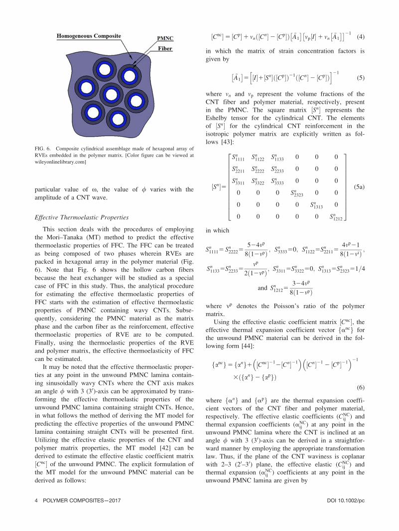
thermoelastic properties of FFC. The FFC can be treated
as being composed of two phases wherein RVEs are
packed in hexagonal array in the polymer material (Fig.
6). Note that Fig. 6 shows the hollow carbon fibers
because the heat exchanger will be studied as a special
case of FFC in this study. Thus, the analytical procedure
for estimating the effective thermoelastic properties of
FFC starts with the estimation of effective thermoelastic
properties of PMNC containing wavy CNTs. Subse-
quently, considering the PMNC material as the matrix
phase and the carbon fiber as the reinforcement, effective
thermoelastic properties of RVE are to be computed.
Finally, using the thermoelastic properties of the RVE
and polymer matrix, the effective thermoelasticity of FFC
can be estimated.
It may be noted that the effective thermoelastic proper-
ties at any point in the unwound PMNC lamina contain-
ing sinusoidally wavy CNTs where the CNT axis makes
an angle / with 3 (30)-axis can be approximated by trans-
forming the effective thermoelastic properties of the
unwound PMNC lamina containing straight CNTs. Hence,
in what follows the method of deriving the MT model for
predicting the effective properties of the unwound PMNC
lamina containing straight CNTs will be presented first.
Utilizing the effective elastic properties of the CNT and
polymer matrix properties, the MT model [42] can be
derived to estimate the effective elastic coefficient matrix
Cnc½ � of the unwound PMNC. The explicit formulation of
the MT model for the unwound PMNC material can be
derived as follows:
Cnc½ �5 Cp½ �1 vn Cn½ �2 Cp½ �ð Þ ~A1
� �vp I½ �1 vn
~A1
� �� �21(4)
in which the matrix of strain concentration factors is
given by
~A1
� �5 I½ �1 Sn½ � Cp½ �ð Þ21 Cn½ �2 Cp½ �ð Þh i21
(5)
where vn and vp represent the volume fractions of the
CNT fiber and polymer material, respectively, present
in the PMNC. The square matrix Sn½ � represents the
Eshelby tensor for the cylindrical CNT. The elements
of Sn½ � for the cylindrical CNT reinforcement in the
isotropic polymer matrix are explicitly written as fol-
lows [43]:
Sn½ �5
Sn1111 Sn
1122 Sn1133 0 0 0
Sn2211 Sn
2222 Sn2233 0 0 0
Sn3311 Sn
3322 Sn3333 0 0 0
0 0 0 Sn2323 0 0
0 0 0 0 Sn1313 0
0 0 0 0 0 Sn1212
2666666666664
3777777777775
(5a)
in which
Sn11115 Sn
22225524mp
8 12mpð Þ ; Sn333350; Sn
11225Sn22115
4mp21
8 12mið Þ ;
Sn11335Sn
22335mp
2 12mpð Þ ; Sn33115Sn
332250; Sn13135Sn
232351=4
and Sn12125
324mp
8 12mpð Þ
where mp denotes the Poisson’s ratio of the polymer
matrix.
Using the effective elastic coefficient matrix Cnc½ �, the
effective thermal expansion coefficient vector ancf g for
the unwound PMNC material can be derived in the fol-
lowing form [44]:
ancf g5 anf g1 Cnc½ �212 Cn½ �21
� �Cn½ �21
2 Cp½ �21� �21
3 anf g2 apf gð Þ(6)
where anf g and apf g are the thermal expansion coeffi-
cient vectors of the CNT fiber and polymer material,
respectively. The effective elastic coefficients (CNCij ) and
thermal expansion coefficients (aNCij ) at any point in the
unwound PMNC lamina where the CNT is inclined at an
angle / with 3 (30)-axis can be derived in a straightfor-
ward manner by employing the appropriate transformation
law. Thus, if the plane of the CNT waviness is coplanar
with 2–3 (20–30) plane, the effective elastic (CNCij ) and
thermal expansion (aNCij ) coefficients at any point in the
unwound PMNC lamina are given by
FIG. 6. Composite cylindrical assemblage made of hexagonal array of
RVEs embedded in the polymer matrix. [Color figure can be viewed at
wileyonlinelibrary.com]
4 POLYMER COMPOSITES—2017 DOI 10.1002/pc
CNC11 5 Cnc
11; CNC12 5 Cnc
12k2 1 Cnc13l2; CNC
13 5 Cnc12l2 1 Cnc
13k2;
CNC22 5 Cnc
22k4 1 Cnc33l4 1 2 Cnc
23 1 2Cnc44
� �k2l2;
CNC23 5 Cnc
22 1 Cnc3324Cnc
44
� �k2l2 1 Cnc
23 k4 1 l4� �
;
CNC33 5 Cnc
22l4 1 Cnc33k4 1 2 Cnc
23 1 2Cnc44
� �k2l2;
CNC44 5 Cnc
22 1 Cnc3322Cnc
2322Cnc44
� �k2l2 1 Cnc
44 k4 1 l4� �
;
CNC55 5 Cnc
55k2 1 Cnc66l2; CNC
66 5 Cnc55l2 1 Cnc
66k2;
aNC11 5 anc
11; aNC22 5anc
22k2 1 anc33l2 and aNC
33 5anc22l2 1 anc
33k2
(7)
in which
k 5 cos/ 5 1 1 npA=Lncos npy=Lnð Þf g2h i21=2
and
l 5 sin/ 5 npA=Lncos npy=Lnð Þ
3 1 1 npA=Lncos npy=Lnð Þf g2h i21=2
Similarly, if the CNT waviness is coplanar with 1–3 (10–30) plane, then CNC
ij and aNCij coefficients at any point of
the unwound PMNC lamina where the CNT is inclined at
an angle / with the 3 (30)-axis are given by
CNC11 5 Cnc
11k4 1 Cnc33l4 1 2 Cnc
13 1 2Cnc55
� �k2l2;
CNC12 5 Cnc
12k2 1 Cnc23l2;
CNC13 5 Cnc
11 1 Cnc3324Cnc
55
� �k2l2 1 Cnc
13 k4 1 l4� �
; CNC22 5 Cnc
22;
CNC23 5 Cnc
12l2 1 Cnc23k2; CNC
33 5 Cnc11l4 1 Cnc
33k4
1 2 Cnc13 1 2Cnc
55
� �k2l2;
CNC44 5Cnc
44k2 1Cnc66l2; CNC
55 5 Cnc11 1Cnc
3322Cnc1322Cnc
55
� �k2l2
1Cnc55 k4 1 l4� �
;
CNC66 5 Cnc
44l2 1 Cnc66k2; aNC
11 5 anc11k2 1 anc
33l2;
aNC22 5 anc
22 and aNC33 5 anc
11l2 1 anc33k2
(8)
It is now obvious that the effective thermoelastic proper-
ties of the unwound PMNC vary along the length of a
CNT as the value of / varies. The average effective elas-
tic coefficient matrix ½ �CNC� and thermal expansion coeffi-
cient vector �aNC
of the lamina of unwound PMNC can
be obtained by averaging the transformed elastic CNCij
� �
and thermal expansion aNCij
� �coefficients over the linear
distance between the CNT ends as follows [45–47]:
��C
NC�5
1
Ln
ðLn
0
CNC� �
dy and �aNC
51
Ln
ðLn
0
aNC
dy
(9)
Note that experiments were also conducted by several
researchers [45–47] to verify the range of validity of such
approximation and good agreement was found between
the analytical results and experimental results. The matrix
½ �CNC� and vector �aNC
provides the effective properties
at a point located in the PMNC where the CNT axis (30-axis) is oriented at an angle h with the 3-axis in 2–3
plane as shown in Figs. 3 and 4. Hence, at any point in
the PMNC surrounding the carbon fiber, the effective
elastic coefficient matrix ½ �CPMNC� and thermal expansion
coefficient vector �aPMNC
of the PMNC with respect to
the 1–2–3 coordinate system turn out to be location
dependent and can be determined by the following
transformations:
�CPMNC
h i5 T½ �2T �C
NCh i
T½ �21and �aPMNC
5 T½ �2T �aNC
(10)
where, T½ �5
1 0 0 0 0 0
0 m2 n2 mn 0 0
0 n2 m2 2mn 0 0
0 22mn 2mn m22n2 0 0
0 0 0 0 m 2n
0 0 0 0 n m
2666666666664
3777777777775
with
m 5 cos h and n 5 sin hFrom Eq. 10, it is obvious that the effective thermo-
elastic properties at any point in the PMNC surrounding
the carbon fiber with respect to the principle material
coordinate (1–2–3) system vary over an annular cross sec-
tion of the PMNC phase. However, without loss of gener-
ality, it may be considered that the volume average of
effective thermoelastic properties over the volume of the
PMNC can be treated as the constant effective elastic
coefficient matrix CPMNC½ � and thermal expansion coeffi-
cient vector aPMNC
containing wavy CNTs surrounding
the carbon fiber with respect to the 1–2–3 coordinate
axes of the FFC and are given by
CPMNC� �
51
p R22a2ð Þ
ð2p
0
ðR
a
�CPMNC
h ir dr dh and
aPMNC
51
p R22a2ð Þ
ð2p
0
ðR
a
�aPMNC
r dr dh (11)
As the RVE is a composite in which the carbon fiber
is the reinforcement and the PMNC is the matrix phase,
the MT model can be employed to estimate its effective
elastic properties. Thus, according to the MT model [42],
the effective elastic coefficient matrix for the RVE is
given by
CRVE� �
5 CPMNC� �
1 �vf Cf� �
2 CPMNC� �� �
~A2
� �vPMNC I½ �½
1 vf~A2
� ��21
(12)
in which the matrix of strain concentration factors are
given by
DOI 10.1002/pc POLYMER COMPOSITES—2017 5
~A2
� �5 I½ �1 Sf
� �CPMNC� �� �21
Cf� �
2 CPMNC� �� �h i21
(13)
where �vf and vPMNC are the volume fractions of carbon
fiber and PMNC, respectively, with respect to the volume
of RVE, and the Eshelby tensor Sf� �
is determined based on
the elastic properties of PMNC and the shape of carbon
fiber. It should be noted that the PMNC material is trans-
versely isotropic and consequently, the Eshelby tensor corre-
sponding to transversely isotropic material is utilized to
compute the matrix Sf� �
. The elements of Sf� �
for the cylin-
drical carbon fiber embedded in the transversely isotropic
PMNC material are explicitly given by [48]
Sf� �
5
Sf1111 Sf
1122 Sf1133 0 0 0
Sf2211 Sf
2222 Sf2233 0 0 0
Sf3311 Sf
3322 Sf3333 0 0 0
0 0 0 Sf2323 0 0
0 0 0 0 Sf1313 0
0 0 0 0 0 Sf1212
2666666666664
3777777777775
(13a)
in which
Sf11115 Sf
222255CPMNC
11 1CPMNC12
8CPMNC11
;
Sf11225 Sf
221153CPMNC
12 2CPMNC11
8CPMNC11
;
Sf11335 Sf
22335CPMNC
13
2CPMNC11
; Sf33115 Sf
332250;
Sf13135 Sf
232351=4
Sf33335 0 and Sf
121253CPMNC
11 2CPMNC12
8CPMNC11
Using the effective elastic coefficient matrix CRVE½ �, ther-
mal expansion coefficient vector aRVEf g for the RVE can
be derived as follows [44]:
aRVE
5 af
1 CRVE� �21
2 Cf� �21
� �
3 Cf� �21
2 CPMNC� �21
� �21
af
2 aPMNC � �
(14)
where Cf� �
and af
are the elastic coefficient matrix
and thermal expansion coefficient vector of the carbon
fiber, respectively. Finally, considering the RVE as the
cylindrical inclusion embedded in the isotropic polymer
matrix (Fig. 6), the effective elastic properties C½ � of the
FFC can be derived as follows:
C½ �5 Cp½ �1vRVE CRVE� �
2 Cp½ �� �
~A3
� ��vP I½ �1vRVE
~A3
� �� �21
(15)
in which the matrix of strain concentration factors are
given by
~A3
� �5 I½ �1 SRVE
� �� �Cp½ �ð Þ21 CRVE
� �2 Cp½ �
� �h i21
(16)
where vRVE and �vp are the volume fractions of RVE and
polymer material, respectively, with respect to the volume
of FFC. The elements of the Eshelby tensor SRVE½ � for
cylindrical RVE reinforcement in the isotropic polymer
matrix are given by [30]
SRVE� �
5
S1111 S1122 S1133 0 0 0
S2211 S2222 S2233 0 0 0
S3311 S3322 S3333 0 0 0
0 0 0 S2323 0 0
0 0 0 0 S1313 0
0 0 0 0 0 S1212
2666666666664
3777777777775
(16a)
in which
S111150; S2222 5S3333 5524mp
8 12mpð Þ ; S2211 5S33115mp
2 12mpð Þ ;
S22335S332254mp21
8 12mpð Þ ; S11225S113350; S13135S121251=4
and S23235324mp
8 12mpð Þ
Finally, the effective thermal expansion coefficient vector
af g for the FFC can be derived as follows [44]:
af g5 aRVE
1 C½ �212 CRVE� �21
� �CRVE� �21
2 Cp½ �21� �21
3 aRVE
2 apf g� �
(17)
Effective Thermal Conductivities
This section deals with the procedures of employing
two modeling approaches; namely, the MOC approach
and effective medium (EM) approach to predict the effec-
tive thermal conductivities of FFC. The various steps
involved in the modeling of thermal conductivities of
FFC are outlined as follows:
� First, the effective thermal conductivities of PMNC are to
be determined using the MOC approach considering the
perfect CNT–polymer matrix interface (i.e., Rk50) or the
EM approach incorporating the CNT–polymer matrix
interfacial thermal resistance (Rk 6¼ 0), where Rk is the
CNT–polymer matrix interfacial thermal resistance.
� Utilizing the thermal conductivities of PMNC and carbon
fiber, the effective thermal conductivities of the RVE are
to be determined using the MOC approach.
� Finally, using the thermal conductivities of RVE and poly-
mer matrix, the effective thermal conductivities of the
FFC can be estimated employing the MOC approach.
6 POLYMER COMPOSITES—2017 DOI 10.1002/pc
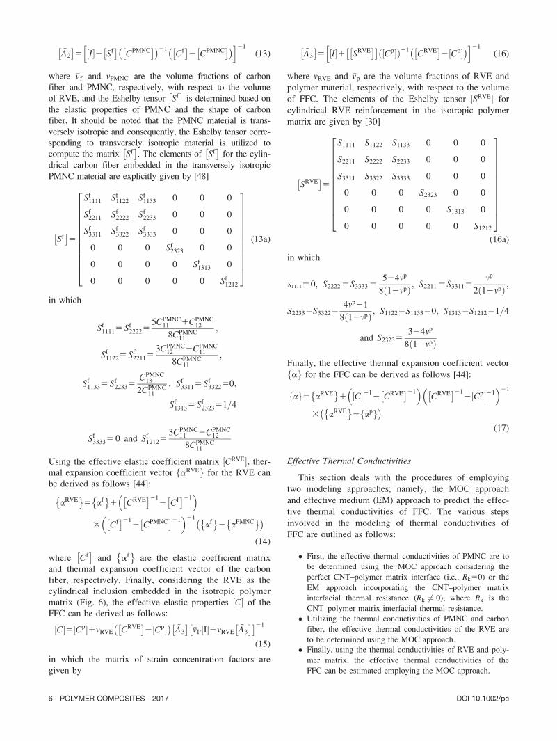
Method of Cells (MOC) Approach. This section
presents the development of MOC approach to estimate
the effective thermal conductivities of the PMNC, RVE,
and FFC. Assuming CNTs as equivalent solid fibers [6,
37–39] and are aligned along the x3-axis, the unwound
PMNC can be viewed to be composed of cells forming
doubly periodic arrays along the x1- and x2-directions.
Figure 7 shows a repeating unit cell (RUC) with four sub-
cells. Each rectangular subcell is labeled by bc, with band c denoting the location of a subcell along the x1- and
x2-directions, respectively. The subcell can be a CNT or
the polymer matrix. Let four local coordinate systems
(�xbð Þ
1 , �xgð Þ
2 , and x3) be introduced, all of which have ori-
gins that are located at the centroid of each cell. In accor-
dance with the MOC approach, the deviation of the
temperature from a reference temperature TR (at which
the material is stress free when its strain is zero), DH(bc),
is expanded in the following form:
DH bcð Þ5DT1�xbð Þ
1 n bcð Þ1 1�x
cð Þ2 n bcð Þ
2 (18)
where n bgð Þ1 and n bgð Þ
2 characterize the linear dependence
of the temperature on the local coordinates. The volume
Vbg
� �of each subcell is
Vbc5bbhcl (19)
where bb, hg, and l denote the width, height, and length
of a subcell, respectively, while the volume Vð Þ of the
RUC is
V5bhl (20)
The continuity conditions of the temperature at the
interfaces of subcells on an average basis lead to the fol-
lowing relations:
h1n1cð Þ
1 1h2n2cð Þ
1 5 h11h2ð Þ @T
@x1
b1nb1ð Þ
2 1b2nb2ð Þ
2 5 b11b2ð Þ @T
@x2
(21)
For the average heat flux in the subcell,
�qbcð Þ
i 52Kbcð Þ
i
@T
@x3
; i51; 2; 3 (22)
where Kbgð Þ
i denotes the thermal conductivities of subcells.
The average heat flux in the unwound PMNC material
is determined from the following relation:
qi51
V
X2
b; c51
Vbc�qbcð Þ
i (23)
The continuity conditions of the heat flux at the interfaces
of subcells yield
�q1cð Þ
1 5�q2cð Þ
1 and �qb1ð Þ
2 5�qb2ð Þ
2 (24)
The average heat flux components are related to the tem-
perature gradients by the effective thermal conductivity
coefficients (Knci ):
�qi52Knci
@T
@x3
(25)
By eliminating the microvariables n bgð Þ1 and n bgð Þ
2 , and
using the continuity conditions, the effective thermal con-
ductivities of unidirectional unwound PMNC lamina are
given by [49]
Knc1 5
Kp Kn h V111V21ð Þ1h2 V121V22ð Þ½ �1Kph1 V121V22ð Þf ghbl Kph11Knh2ð Þ ;
Knc2 5
Kp Kn b V111V12ð Þ1b2 V211V22ð Þ½ �1Kpb1 V211V22ð Þf ghbl Kpb11Knb2ð Þ and
Knc3 5
KnV111Kp V121V211V22ð Þhbl
(26)
The effective thermal conductivities (KNCi ) at any point in
the unwound PMNC lamina where the CNT is inclined at
an angle / with the 3 (30)-axis can be derived in a
straightforward manner by employing the appropriate
transformation law as follows:
KNC� �
5 T1½ �2T Knc½ � T1½ �21and KNC� �
5 T2½ �2T Knc½ � T2½ �21
(27)
accordingly as the CNT waviness is coplanar with 2–3
(20–30) or 1–3 (10–30) plane, respectively. The various
matrices appeared in Eq. 27 are given by
FIG. 7. Repeating unit cell of the unwound PMNC material with four
subcells (b, c 5 1, 2). [Color figure can be viewed at wileyonlinelibrary.
com]
DOI 10.1002/pc POLYMER COMPOSITES—2017 7
Knc½ �5
Knc1 0 0
0 Knc2 0
0 0 Knc3
26664
37775; T1½ �5
1 0 0
0 cos/ sin/
0 2sin/ cos/
26664
37775
and T2½ �5
cos/ 0 sin/
0 1 0
2sin/ 0 cos/
26664
37775
Following the procedure for deriving the effective elastic
coefficient matrix CPMNC½ �, the effective thermal conduc-
tivity matrix KPMNC½ � can be obtained as follows:
�KNC
h i5
1
Ln
ðLn
0
KNC� �
dy (28)
�KPMNC
h i5
1 0 0
0 cosh sinh
0 2sinh cosh
26664
37775
2TKnc
1 0 0
0 Knc2 0
0 0 Knc3
26664
37775
1 0 0
0 cosh sinh
0 2sinh cosh
26664
37775
21
(29)
KPMNC� �
51
p R22a2ð Þ
ð2p
0
ðR
a
�KPMNC
h ir dr dh (30)
It is worthwhile to note that the thermal conductivity matrix
of the homogenized PMNC KPMNC½ � is transversely isotropic
and its axis of transverse isotropy is the 1- or x1-axis. To
model the RVE by the MOC approach, the RVE is consid-
ered to be composed of cells periodically arranged along the
x2- and x3-directions while each cell consists of bg number
of subcells. In this case, each RUC represents the RVE and a
subcell is composed of carbon fiber or PMNC. Finally, the
MOC approach for the RVE can be augmented in a straight-
forward manner to estimate the effective thermal conductivi-
ties of FFC in which the polymer is the matrix material and
the RVE is the reinforcement along the 1- or x1-direction.
Effective Medium (EM) Approach. This section
presents the Maxwell Garnett type EM approach to esti-
mate the effective thermal conductivities of the PMNC
incorporating the CNT–polymer matrix interfacial thermal
resistance. Assuming CNTs as solid fibers [6, 37–39], the
EM approach by Nan et al. [50] can be augmented to pre-
dict the effective thermal conductivities (Knci ) of unwound
PMNC material with straight CNTs and are given by
Knc1 5Knc
2 5Kp Kn 11að Þ1Kp1vn Kn 12að Þ2Kp½ �Kn 11að Þ1Kp2vn Kn 12að Þ2Kp½ �
and Knc3 5vnKn1vpKp
(31)
In Eq. 31, a dimensionless parameter a 5 2ak=dn in
which the interfacial thermal property is concentrated on
a surface of zero thickness and is characterized by Kap-
tiza radius, ak5RkKp, where dn represents the CNT diam-
eter. Once Knc½ � is computed, Eqs. 27–30 are used to
estimate the effective thermal conductivities of the
PMNC material surrounding the carbon fiber.
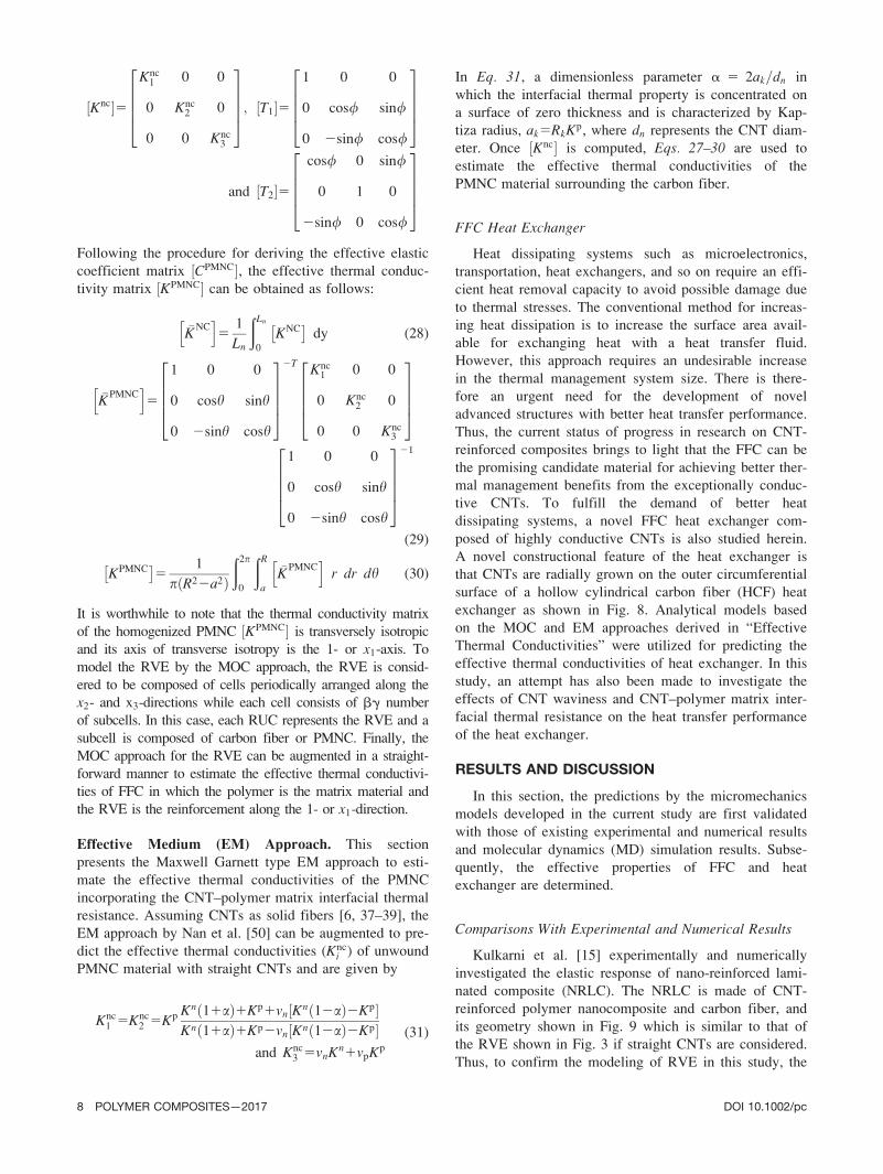
FFC Heat Exchanger
Heat dissipating systems such as microelectronics,
transportation, heat exchangers, and so on require an effi-
cient heat removal capacity to avoid possible damage due
to thermal stresses. The conventional method for increas-
ing heat dissipation is to increase the surface area avail-
able for exchanging heat with a heat transfer fluid.
However, this approach requires an undesirable increase
in the thermal management system size. There is there-
fore an urgent need for the development of novel
advanced structures with better heat transfer performance.
Thus, the current status of progress in research on CNT-
reinforced composites brings to light that the FFC can be
the promising candidate material for achieving better ther-
mal management benefits from the exceptionally conduc-
tive CNTs. To fulfill the demand of better heat
dissipating systems, a novel FFC heat exchanger com-
posed of highly conductive CNTs is also studied herein.
A novel constructional feature of the heat exchanger is
that CNTs are radially grown on the outer circumferential
surface of a hollow cylindrical carbon fiber (HCF) heat
exchanger as shown in Fig. 8. Analytical models based
on the MOC and EM approaches derived in “Effective
Thermal Conductivities” were utilized for predicting the
effective thermal conductivities of heat exchanger. In this
study, an attempt has also been made to investigate the
effects of CNT waviness and CNT–polymer matrix inter-
facial thermal resistance on the heat transfer performance
of the heat exchanger.
RESULTS AND DISCUSSION
In this section, the predictions by the micromechanics
models developed in the current study are first validated
with those of existing experimental and numerical results
and molecular dynamics (MD) simulation results. Subse-
quently, the effective properties of FFC and heat
exchanger are determined.
Comparisons With Experimental and Numerical Results
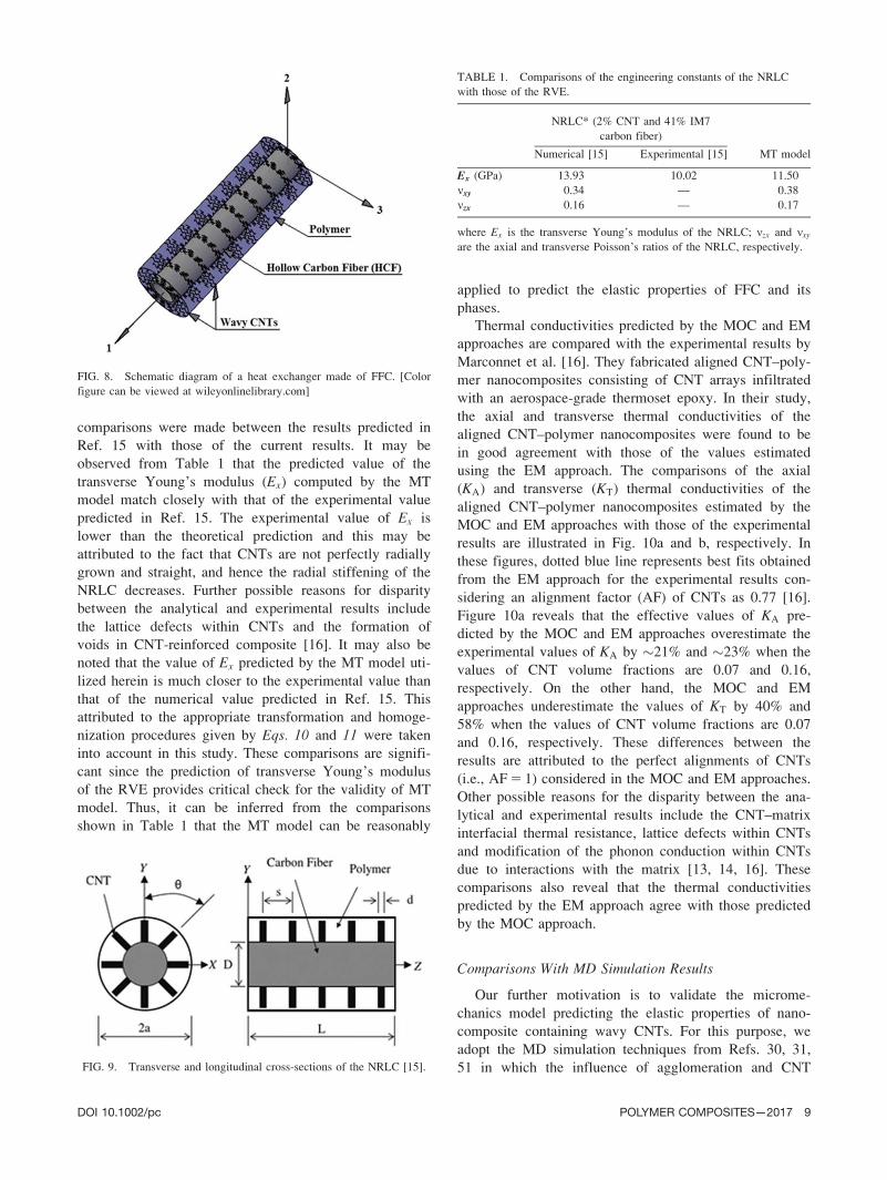
Kulkarni et al. [15] experimentally and numerically
investigated the elastic response of nano-reinforced lami-
nated composite (NRLC). The NRLC is made of CNT-
reinforced polymer nanocomposite and carbon fiber, and
its geometry shown in Fig. 9 which is similar to that of
the RVE shown in Fig. 3 if straight CNTs are considered.
Thus, to confirm the modeling of RVE in this study, the
8 POLYMER COMPOSITES—2017 DOI 10.1002/pc
comparisons were made between the results predicted in
Ref. 15 with those of the current results. It may be
observed from Table 1 that the predicted value of the
transverse Young’s modulus (Ex) computed by the MT
model match closely with that of the experimental value
predicted in Ref. 15. The experimental value of Ex is
lower than the theoretical prediction and this may be
attributed to the fact that CNTs are not perfectly radially
grown and straight, and hence the radial stiffening of the
NRLC decreases. Further possible reasons for disparity
between the analytical and experimental results include
the lattice defects within CNTs and the formation of
voids in CNT-reinforced composite [16]. It may also be
noted that the value of Ex predicted by the MT model uti-
lized herein is much closer to the experimental value than
that of the numerical value predicted in Ref. 15. This
attributed to the appropriate transformation and homoge-
nization procedures given by Eqs. 10 and 11 were taken
into account in this study. These comparisons are signifi-
cant since the prediction of transverse Young’s modulus
of the RVE provides critical check for the validity of MT
model. Thus, it can be inferred from the comparisons
shown in Table 1 that the MT model can be reasonably
applied to predict the elastic properties of FFC and its
phases.
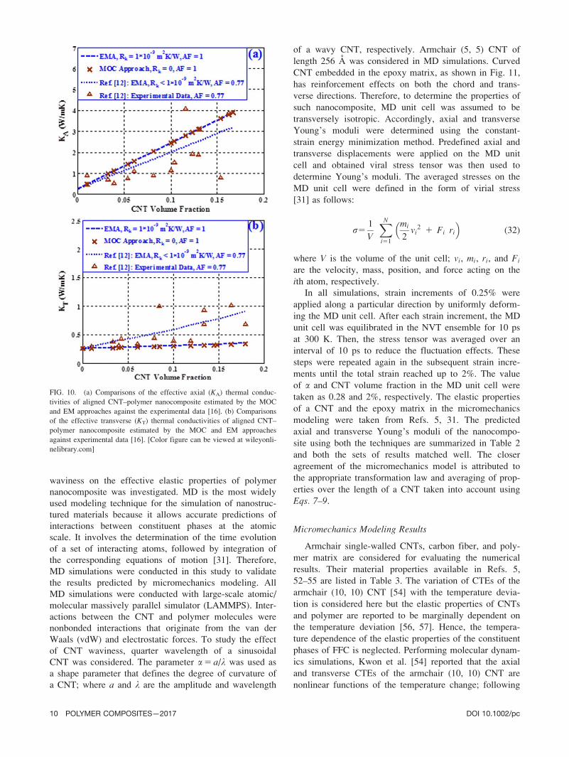
Thermal conductivities predicted by the MOC and EM
approaches are compared with the experimental results by
Marconnet et al. [16]. They fabricated aligned CNT–poly-
mer nanocomposites consisting of CNT arrays infiltrated
with an aerospace-grade thermoset epoxy. In their study,
the axial and transverse thermal conductivities of the
aligned CNT–polymer nanocomposites were found to be
in good agreement with those of the values estimated
using the EM approach. The comparisons of the axial
(KA) and transverse (KT) thermal conductivities of the
aligned CNT–polymer nanocomposites estimated by the
MOC and EM approaches with those of the experimental
results are illustrated in Fig. 10a and b, respectively. In
these figures, dotted blue line represents best fits obtained
from the EM approach for the experimental results con-
sidering an alignment factor (AF) of CNTs as 0.77 [16].
Figure 10a reveals that the effective values of KA pre-
dicted by the MOC and EM approaches overestimate the
experimental values of KA by �21% and �23% when the
values of CNT volume fractions are 0.07 and 0.16,
respectively. On the other hand, the MOC and EM
approaches underestimate the values of KT by 40% and
58% when the values of CNT volume fractions are 0.07
and 0.16, respectively. These differences between the
results are attributed to the perfect alignments of CNTs
(i.e., AF 5 1) considered in the MOC and EM approaches.
Other possible reasons for the disparity between the ana-
lytical and experimental results include the CNT–matrix
interfacial thermal resistance, lattice defects within CNTs
and modification of the phonon conduction within CNTs
due to interactions with the matrix [13, 14, 16]. These
comparisons also reveal that the thermal conductivities
predicted by the EM approach agree with those predicted
by the MOC approach.
Comparisons With MD Simulation Results
Our further motivation is to validate the microme-
chanics model predicting the elastic properties of nano-
composite containing wavy CNTs. For this purpose, we
adopt the MD simulation techniques from Refs. 30, 31,
51 in which the influence of agglomeration and CNT
FIG. 8. Schematic diagram of a heat exchanger made of FFC. [Color
figure can be viewed at wileyonlinelibrary.com]
FIG. 9. Transverse and longitudinal cross-sections of the NRLC [15].
TABLE 1. Comparisons of the engineering constants of the NRLC
with those of the RVE.
NRLC* (2% CNT and 41% IM7
carbon fiber)
Numerical [15] Experimental [15] MT model
Ex (GPa) 13.93 10.02 11.50
mxy 0.34 — 0.38
mzx 0.16 — 0.17
where Ex is the transverse Young’s modulus of the NRLC; mzx and mxy
are the axial and transverse Poisson’s ratios of the NRLC, respectively.
DOI 10.1002/pc POLYMER COMPOSITES—2017 9
waviness on the effective elastic properties of polymer
nanocomposite was investigated. MD is the most widely
used modeling technique for the simulation of nanostruc-
tured materials because it allows accurate predictions of
interactions between constituent phases at the atomic
scale. It involves the determination of the time evolution
of a set of interacting atoms, followed by integration of
the corresponding equations of motion [31]. Therefore,
MD simulations were conducted in this study to validate
the results predicted by micromechanics modeling. All
MD simulations were conducted with large-scale atomic/
molecular massively parallel simulator (LAMMPS). Inter-
actions between the CNT and polymer molecules were
nonbonded interactions that originate from the van der
Waals (vdW) and electrostatic forces. To study the effect
of CNT waviness, quarter wavelength of a sinusoidal
CNT was considered. The parameter a 5 a/k was used as
a shape parameter that defines the degree of curvature of
a CNT; where a and k are the amplitude and wavelength
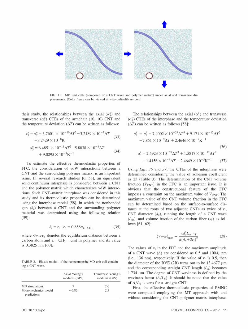
of a wavy CNT, respectively. Armchair (5, 5) CNT of
length 256 A was considered in MD simulations. Curved
CNT embedded in the epoxy matrix, as shown in Fig. 11,
has reinforcement effects on both the chord and trans-
verse directions. Therefore, to determine the properties of
such nanocomposite, MD unit cell was assumed to be
transversely isotropic. Accordingly, axial and transverse
Young’s moduli were determined using the constant-
strain energy minimization method. Predefined axial and
transverse displacements were applied on the MD unit
cell and obtained viral stress tensor was then used to
determine Young’s moduli. The averaged stresses on the
MD unit cell were defined in the form of virial stress
[31] as follows:
r51
V
XN
i51
mi
2vi
2 1 Fi ri
� �(32)
where V is the volume of the unit cell; vi, mi, ri, and Fi
are the velocity, mass, position, and force acting on the
ith atom, respectively.
In all simulations, strain increments of 0.25% were
applied along a particular direction by uniformly deform-
ing the MD unit cell. After each strain increment, the MD
unit cell was equilibrated in the NVT ensemble for 10 ps
at 300 K. Then, the stress tensor was averaged over an
interval of 10 ps to reduce the fluctuation effects. These
steps were repeated again in the subsequent strain incre-
ments until the total strain reached up to 2%. The value
of a and CNT volume fraction in the MD unit cell were
taken as 0.28 and 2%, respectively. The elastic properties
of a CNT and the epoxy matrix in the micromechanics
modeling were taken from Refs. 5, 31. The predicted
axial and transverse Young’s moduli of the nanocompo-
site using both the techniques are summarized in Table 2
and both the sets of results matched well. The closer
agreement of the micromechanics model is attributed to
the appropriate transformation law and averaging of prop-
erties over the length of a CNT taken into account using
Eqs. 7–9.
Micromechanics Modeling Results
Armchair single-walled CNTs, carbon fiber, and poly-
mer matrix are considered for evaluating the numerical
results. Their material properties available in Refs. 5,
52–55 are listed in Table 3. The variation of CTEs of the
armchair (10, 10) CNT [54] with the temperature devia-
tion is considered here but the elastic properties of CNTs
and polymer are reported to be marginally dependent on
the temperature deviation [56, 57]. Hence, the tempera-
ture dependence of the elastic properties of the constituent
phases of FFC is neglected. Performing molecular dynam-
ics simulations, Kwon et al. [54] reported that the axial
and transverse CTEs of the armchair (10, 10) CNT are
nonlinear functions of the temperature change; following
FIG. 10. (a) Comparisons of the effective axial (KA) thermal conduc-
tivities of aligned CNT–polymer nanocomposite estimated by the MOC
and EM approaches against the experimental data [16]. (b) Comparisons
of the effective transverse (KT) thermal conductivities of aligned CNT–
polymer nanocomposite estimated by the MOC and EM approaches
against experimental data [16]. [Color figure can be viewed at wileyonli-
nelibrary.com]
10 POLYMER COMPOSITES—2017 DOI 10.1002/pc
their study, the relationships between the axial (an3) and
transverse (an1) CTEs of the armchair (10, 10) CNT and
the temperature deviation (DT) can be written as follows:
an1 5 an
2 5 3:7601 3 10210DT223:2189 3 1027DT
23:2429 3 1028K21(33)
an3 5 6:4851 3 10211DT225:8038 3 1028DT
1 9:0295 3 1028K21(34)
To estimate the effective thermoelastic properties of
FFC, the consideration of vdW interactions between a
CNT and the surrounding polymer matrix, is an important
issue. In several research studies [6, 58], an equivalent
solid continuum interphase is considered between a CNT
and the polymer matrix which characterizes vdW interac-
tions. Such CNT–matrix interphase was considered in this
study and its thermoelastic properties can be determined
using the interphase model [58], in which the nonbonded
gap (hi) between a CNT and the surrounding polymer
material was determined using the following relation
[59]:
hi 5 ri2rn 5 0:858rC2CH2(35)
where rC2CH2denotes the equilibrium distance between a
carbon atom and a ACH2A unit in polymer and its value
is 0.3825 nm [60].
The relationships between the axial (ai1) and transverse
(ai3) CTEs of the interphase and the temperature deviation
(DT) can be written as follows [58]:
ai1 5 ai
2 5 7:4002 3 10229DT3 1 9:171 3 10212DT2
27:851 3 1029DT 1 2:4646 3 1025K21
(36)
ai3 5 2:5923 3 10228DT3 1 1:5817 3 10212DT2
21:4156 3 1029DT 1 2:4649 3 1025K21 (37)
Using Eqs. 36 and 37, the CTEs of the interphase were
determined considering the value of adhesion coefficient
as 25 (Table 3). The determination of the CNT volume
fraction VCNTð Þ in the FFC is an important issue. It is
obvious that the constructional feature of the FFC
imposes a constraint on the maximum value of VCNT. The
maximum value of the CNT volume fraction in the FFC
can be determined based on the surface-to-surface dis-
tance at the roots of two adjacent CNTs as twice of ri,
CNT diameter (dn), running the length of a CNT wave
(Lnr), and volume fraction of the carbon fiber (vf) as fol-
lows [61, 62]:
VCNTð Þmax 5pd2
nLnr vf
d dn12rið Þ2(38)
The values of vf in the FFC and the maximum amplitude
of a CNT wave (A) are considered as 0.5 and 100dn nm
(i.e., 136 nm), respectively. If the value of vf is 0.5, then
the diameter of the RVE (2R) turns out to be 13.4677 mm
and the corresponding straight CNT length (Ln) becomes
1.734 mm. The degree of CNT waviness is defined by the
waviness factor (A=LnÞ. It should be noted that the value
of A=Ln is zero for a straight CNT.
First, the effective thermoelastic properties of PMNC
were computed employing the MT approach with and
without considering the CNT–polymer matrix interphase.
FIG. 11. MD unit cells (composed of a CNT wave and polymer matrix) under axial and transverse dis-
placements. [Color figure can be viewed at wileyonlinelibrary.com]
TABLE 2. Elastic moduli of the nanocomposite MD unit cell contain-
ing a CNT wave.
Axial Young’s
modulus (GPa)
Transverse Young’s
modulus (GPa)
MD simulations 7 2.6
Micromechanics model
predictions
�6.85 2.5
DOI 10.1002/pc POLYMER COMPOSITES—2017 11
In case of former, a CNT coated with interphase was
homogenized as an equivalent solid nanofiber using
Eq. 4. Such a nanofiber can be viewed as a composite in
which a CNT is the reinforcement and the interphase
material plays the role of a matrix. Subsequently, the
PMNC was assumed to be comprised of a nanofiber
embedded in the polymer matrix. The estimated effective
thermomechanical properties of PMNC were then used to
compute the effective thermomechanical properties of
RVE. However, for the sake of brevity, the effective ther-
momechanical properties of the nanofiber, PMNC, and
RVE are not presented here. The variations of the ampli-
tudes of CNT waves are considered for the particular
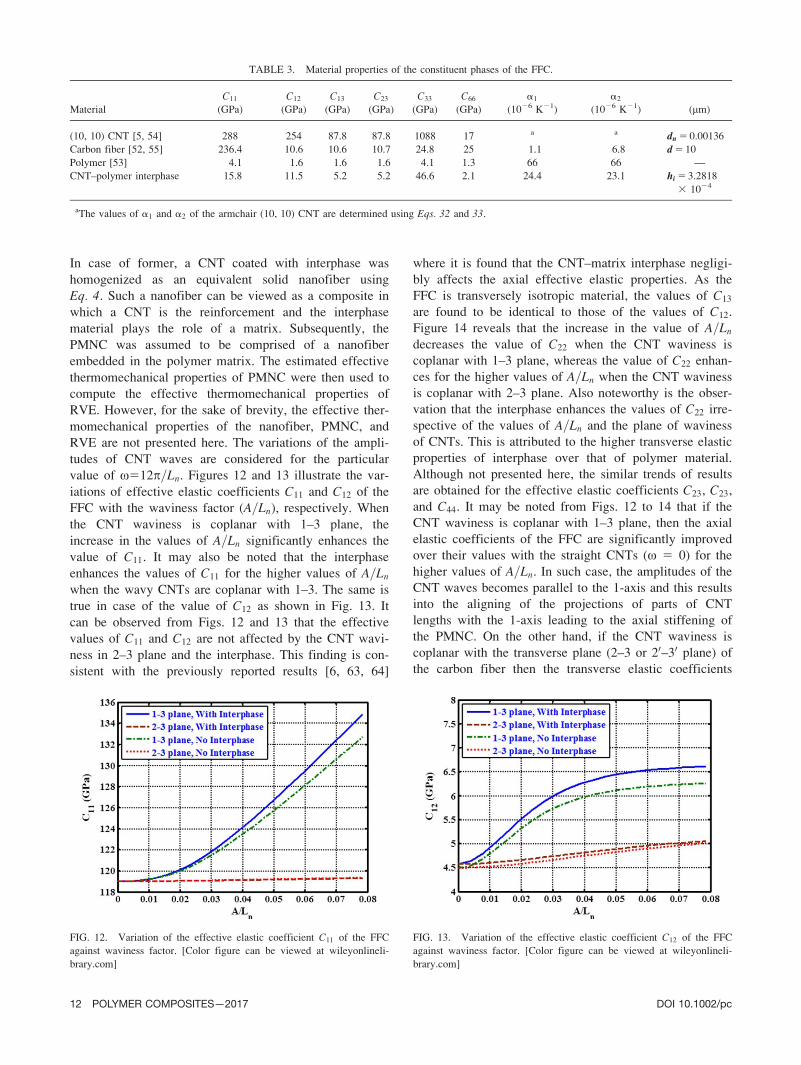
value of x512p=Ln. Figures 12 and 13 illustrate the var-
iations of effective elastic coefficients C11 and C12 of the
FFC with the waviness factor (A=Ln), respectively. When
the CNT waviness is coplanar with 1–3 plane, the
increase in the values of A=Ln significantly enhances the
value of C11. It may also be noted that the interphase
enhances the values of C11 for the higher values of A=Ln
when the wavy CNTs are coplanar with 1–3. The same is
true in case of the value of C12 as shown in Fig. 13. It
can be observed from Figs. 12 and 13 that the effective
values of C11 and C12 are not affected by the CNT wavi-
ness in 2–3 plane and the interphase. This finding is con-
sistent with the previously reported results [6, 63, 64]
where it is found that the CNT–matrix interphase negligi-
bly affects the axial effective elastic properties. As the
FFC is transversely isotropic material, the values of C13
are found to be identical to those of the values of C12.
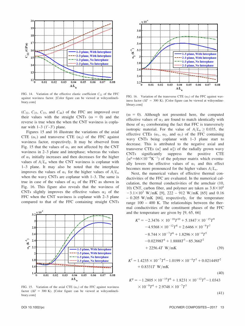
Figure 14 reveals that the increase in the value of A=Ln
decreases the value of C22 when the CNT waviness is
coplanar with 1–3 plane, whereas the value of C22 enhan-
ces for the higher values of A=Ln when the CNT waviness
is coplanar with 2–3 plane. Also noteworthy is the obser-
vation that the interphase enhances the values of C22 irre-
spective of the values of A=Ln and the plane of waviness
of CNTs. This is attributed to the higher transverse elastic
properties of interphase over that of polymer material.
Although not presented here, the similar trends of results
are obtained for the effective elastic coefficients C23, C23,
and C44. It may be noted from Figs. 12 to 14 that if the
CNT waviness is coplanar with 1–3 plane, then the axial
elastic coefficients of the FFC are significantly improved
over their values with the straight CNTs (x 5 0) for the
higher values of A=Ln. In such case, the amplitudes of the
CNT waves becomes parallel to the 1-axis and this results
into the aligning of the projections of parts of CNT
lengths with the 1-axis leading to the axial stiffening of
the PMNC. On the other hand, if the CNT waviness is
coplanar with the transverse plane (2–3 or 20–30 plane) of
the carbon fiber then the transverse elastic coefficients
TABLE 3. Material properties of the constituent phases of the FFC.
Material
C11
(GPa)
C12
(GPa)
C13
(GPa)
C23
(GPa)
C33
(GPa)
C66
(GPa)
a1
(1026 K21)
a2
(1026 K21) (mm)
(10, 10) CNT [5, 54] 288 254 87.8 87.8 1088 17 a a dn 5 0.00136
Carbon fiber [52, 55] 236.4 10.6 10.6 10.7 24.8 25 1.1 6.8 d 5 10
Polymer [53] 4.1 1.6 1.6 1.6 4.1 1.3 66 66 —
CNT–polymer interphase 15.8 11.5 5.2 5.2 46.6 2.1 24.4 23.1 hi 5 3.2818
3 1024
aThe values of a1 and a2 of the armchair (10, 10) CNT are determined using Eqs. 32 and 33.
FIG. 12. Variation of the effective elastic coefficient C11 of the FFC
against waviness factor. [Color figure can be viewed at wileyonlineli-
brary.com]
FIG. 13. Variation of the effective elastic coefficient C12 of the FFC
against waviness factor. [Color figure can be viewed at wileyonlineli-
brary.com]
12 POLYMER COMPOSITES—2017 DOI 10.1002/pc
(C22, C23, C33, and C44) of the FFC are improved over
their values with the straight CNTs (x 5 0) and the
reverse is true when the when the CNT waviness is copla-
nar with 1–3 (10–30) plane.
Figures 15 and 16 illustrate the variations of the axial
CTE (a1) and transverse CTE (a2) of the FFC against
waviness factor, respectively. It may be observed from
Fig. 15 that the values of a1 are not affected by the CNT
waviness in 2–3 plane and interphase; whereas the values
of a1 initially increases and then decreases for the higher
values of A=Ln when the CNT waviness is coplanar with
1–3 plane. It may also be noted that the interphase
improves the values of a1 for the higher values of A=Ln
when the wavy CNTs are coplanar with 1–3. The same is
true in case of the values of a2 of the FFC as shown in
Fig. 16. This figure also reveals that the waviness of
CNTs slightly improves the effective values a2 of the
FFC when the CNT waviness is coplanar with 2–3 plane
compared to that of the FFC containing straight CNTs
(x 5 0). Although not presented here, the computed
effective values of a3 are found to match identically with
those of a2 corroborating the fact that FFC is transversely
isotropic material. For the value of A=Ln � 0:035, the
effective CTEs (a1, a2, and a3) of the FFC containing
wavy CNTs being coplanar with 1–3 plane start to
decrease. This is attributed to the negative axial and
transverse CTEs (an1 and an
3) of the radially grown wavy
CNTs significantly suppress the positive CTE
ap56631026K21�
) of the polymer matrix which eventu-
ally lowers the effective values of a1 and this effect
becomes more pronounced for the higher values A=Ln.
Next, the numerical values of effective thermal con-
ductivities of the FFC are evaluated. In the numerical cal-
culation, the thermal conductivities of the armchair (10,
10) CNT, carbon fiber, and polymer are taken as 3:83104
23:13103 W=mK [9], 222 – 912 W=mK [65] and 0:16
– 0:205 W=mK [66], respectively, for the temperature
range 100 – 400 K. The relationships between the ther-
mal conductivities of the constituent phases of the FFC
and the temperature are given by [9, 65, 66]
Kn 5 22:3476 3 10218T10 1 5:1847 3 10215T9
24:9368 3 10212T8 1 2:6466 3 1029T7
28:744 3 1027T6 1 1:8296 3 1024T5
20:02398T4 1 1:8888T3285:366T2
1 2256:4T W=mK (39)
Kf 5 1:4235 3 1027T421:0199 3 1024T3 1 0:021449T2
1 0:8331T W=mK
(40)
Kp 5 21:2805 3 10215T6 1 1:8231 3 10212T521:0343
3 1029T4 1 2:9748 3 1027T3
(41)
FIG. 14. Variation of the effective elastic coefficient C22 of the FFC
against waviness factor. [Color figure can be viewed at wileyonlineli-
brary.com]
FIG. 15. Variation of the axial CTE (a1) of the FFC against waviness
factor (DT 5 300 K). [Color figure can be viewed at wileyonlineli-
brary.com]
FIG. 16. Variation of the transverse CTE (a2) of the FFC against wav-
iness factor (DT 5 300 K). [Color figure can be viewed at wileyonline-
library.com]
DOI 10.1002/pc POLYMER COMPOSITES—2017 13
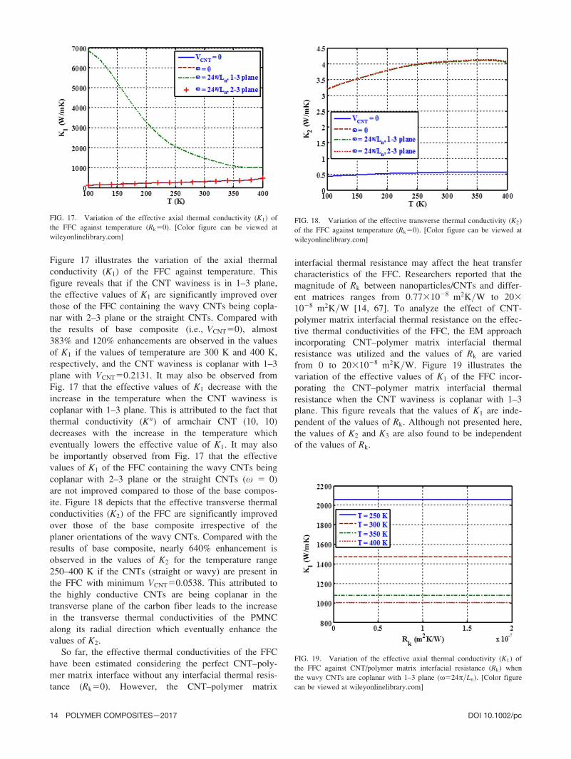
Figure 17 illustrates the variation of the axial thermal
conductivity (K1) of the FFC against temperature. This
figure reveals that if the CNT waviness is in 1–3 plane,
the effective values of K1 are significantly improved over
those of the FFC containing the wavy CNTs being copla-
nar with 2–3 plane or the straight CNTs. Compared with
the results of base composite (i.e., VCNT50), almost
383% and 120% enhancements are observed in the values
of K1 if the values of temperature are 300 K and 400 K,
respectively, and the CNT waviness is coplanar with 1–3
plane with VCNT50:2131. It may also be observed from
Fig. 17 that the effective values of K1 decrease with the
increase in the temperature when the CNT waviness is
coplanar with 1–3 plane. This is attributed to the fact that
thermal conductivity (Kn) of armchair CNT (10, 10)
decreases with the increase in the temperature which
eventually lowers the effective value of K1. It may also
be importantly observed from Fig. 17 that the effective
values of K1 of the FFC containing the wavy CNTs being
coplanar with 2–3 plane or the straight CNTs (x 5 0)
are not improved compared to those of the base compos-
ite. Figure 18 depicts that the effective transverse thermal
conductivities (K2) of the FFC are significantly improved
over those of the base composite irrespective of the
planer orientations of the wavy CNTs. Compared with the
results of base composite, nearly 640% enhancement is
observed in the values of K2 for the temperature range
250–400 K if the CNTs (straight or wavy) are present in
the FFC with minimum VCNT50:0538. This attributed to
the highly conductive CNTs are being coplanar in the
transverse plane of the carbon fiber leads to the increase
in the transverse thermal conductivities of the PMNC
along its radial direction which eventually enhance the
values of K2.
So far, the effective thermal conductivities of the FFC
have been estimated considering the perfect CNT–poly-
mer matrix interface without any interfacial thermal resis-
tance (Rk50). However, the CNT–polymer matrix
interfacial thermal resistance may affect the heat transfer
characteristics of the FFC. Researchers reported that the
magnitude of Rk between nanoparticles/CNTs and differ-
ent matrices ranges from 0:7731028 m2K=W to 203
1028 m2K=W [14, 67]. To analyze the effect of CNT-
polymer matrix interfacial thermal resistance on the effec-
tive thermal conductivities of the FFC, the EM approach
incorporating CNT–polymer matrix interfacial thermal
resistance was utilized and the values of Rk are varied
from 0 to 2031028 m2K=W. Figure 19 illustrates the
variation of the effective values of K1 of the FFC incor-
porating the CNT–polymer matrix interfacial thermal
resistance when the CNT waviness is coplanar with 1–3
plane. This figure reveals that the values of K1 are inde-
pendent of the values of Rk. Although not presented here,
the values of K2 and K3 are also found to be independent
of the values of Rk.
FIG. 17. Variation of the effective axial thermal conductivity (K1) of
the FFC against temperature (Rk50). [Color figure can be viewed at
wileyonlinelibrary.com]
FIG. 18. Variation of the effective transverse thermal conductivity (K2)
of the FFC against temperature (Rk50). [Color figure can be viewed at
wileyonlinelibrary.com]
FIG. 19. Variation of the effective axial thermal conductivity (K1) of
the FFC against CNT/polymer matrix interfacial resistance (Rk) when
the wavy CNTs are coplanar with 1–3 plane (x524p=Ln). [Color figure
can be viewed at wileyonlinelibrary.com]
14 POLYMER COMPOSITES—2017 DOI 10.1002/pc
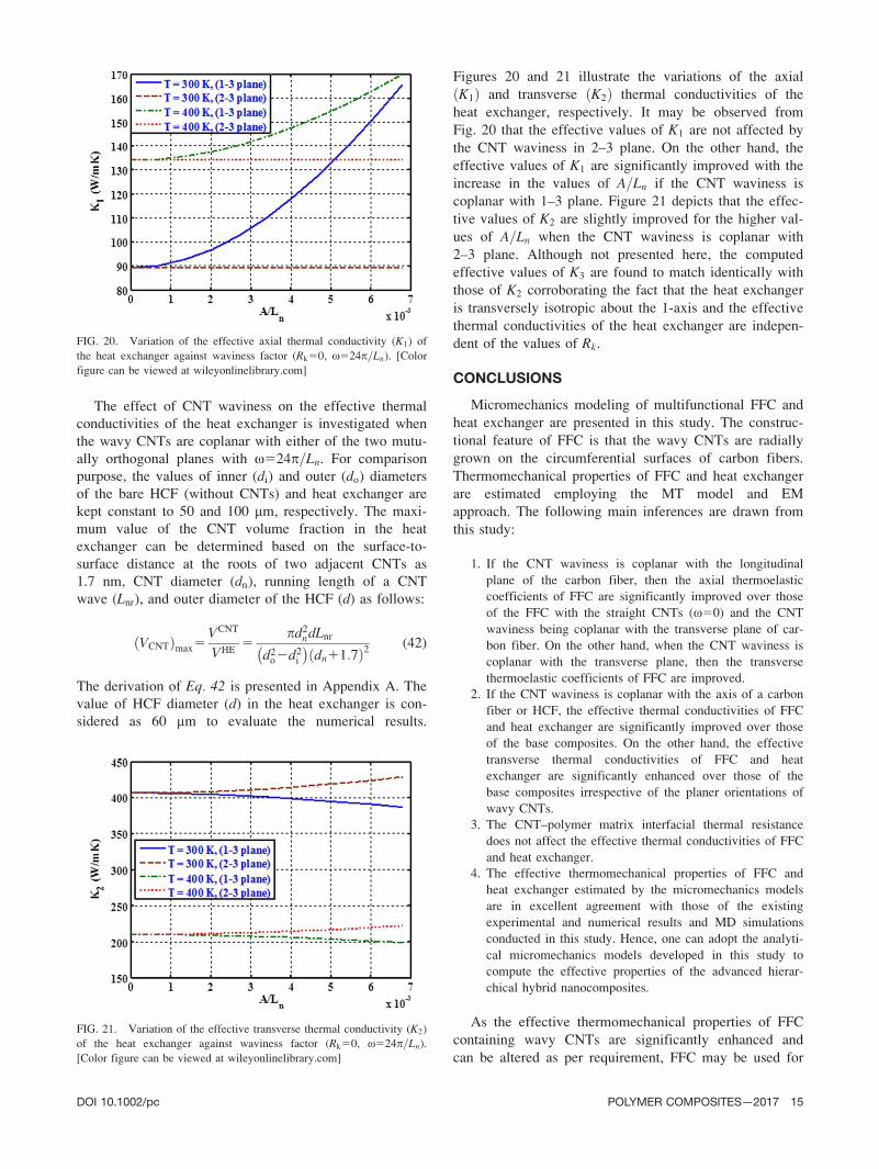
The effect of CNT waviness on the effective thermal
conductivities of the heat exchanger is investigated when
the wavy CNTs are coplanar with either of the two mutu-
ally orthogonal planes with x524p=Ln. For comparison
purpose, the values of inner (di) and outer (do) diameters
of the bare HCF (without CNTs) and heat exchanger are
kept constant to 50 and 100 mm, respectively. The maxi-
mum value of the CNT volume fraction in the heat
exchanger can be determined based on the surface-to-
surface distance at the roots of two adjacent CNTs as
1.7 nm, CNT diameter (dn), running length of a CNT
wave (Lnr), and outer diameter of the HCF (d) as follows:
VCNTð Þmax5VCNT
VHE5
pd2ndLnr
d2o2d2
i
� �dn11:7ð Þ2
(42)
The derivation of Eq. 42 is presented in Appendix A. The
value of HCF diameter (d) in the heat exchanger is con-
sidered as 60 mm to evaluate the numerical results.
Figures 20 and 21 illustrate the variations of the axial
K1ð Þ and transverse K2ð Þ thermal conductivities of the
heat exchanger, respectively. It may be observed from
Fig. 20 that the effective values of K1 are not affected by
the CNT waviness in 2–3 plane. On the other hand, the
effective values of K1 are significantly improved with the
increase in the values of A=Ln if the CNT waviness is
coplanar with 1–3 plane. Figure 21 depicts that the effec-
tive values of K2 are slightly improved for the higher val-
ues of A=Ln when the CNT waviness is coplanar with
2–3 plane. Although not presented here, the computed
effective values of K3 are found to match identically with
those of K2 corroborating the fact that the heat exchanger
is transversely isotropic about the 1-axis and the effective
thermal conductivities of the heat exchanger are indepen-
dent of the values of Rk.
CONCLUSIONS
Micromechanics modeling of multifunctional FFC and
heat exchanger are presented in this study. The construc-
tional feature of FFC is that the wavy CNTs are radially
grown on the circumferential surfaces of carbon fibers.
Thermomechanical properties of FFC and heat exchanger
are estimated employing the MT model and EM
approach. The following main inferences are drawn from
this study:
1. If the CNT waviness is coplanar with the longitudinal
plane of the carbon fiber, then the axial thermoelastic
coefficients of FFC are significantly improved over those
of the FFC with the straight CNTs (x50) and the CNT
waviness being coplanar with the transverse plane of car-
bon fiber. On the other hand, when the CNT waviness is
coplanar with the transverse plane, then the transverse
thermoelastic coefficients of FFC are improved.
2. If the CNT waviness is coplanar with the axis of a carbon
fiber or HCF, the effective thermal conductivities of FFC
and heat exchanger are significantly improved over those
of the base composites. On the other hand, the effective
transverse thermal conductivities of FFC and heat
exchanger are significantly enhanced over those of the
base composites irrespective of the planer orientations of
wavy CNTs.
3. The CNT–polymer matrix interfacial thermal resistance
does not affect the effective thermal conductivities of FFC
and heat exchanger.
4. The effective thermomechanical properties of FFC and
heat exchanger estimated by the micromechanics models
are in excellent agreement with those of the existing
experimental and numerical results and MD simulations
conducted in this study. Hence, one can adopt the analyti-
cal micromechanics models developed in this study to
compute the effective properties of the advanced hierar-
chical hybrid nanocomposites.
As the effective thermomechanical properties of FFC
containing wavy CNTs are significantly enhanced and
can be altered as per requirement, FFC may be used for
FIG. 20. Variation of the effective axial thermal conductivity (K1) of
the heat exchanger against waviness factor (Rk50, x524p=Ln). [Color
figure can be viewed at wileyonlinelibrary.com]
FIG. 21. Variation of the effective transverse thermal conductivity (K2)
of the heat exchanger against waviness factor (Rk50, x524p=Ln).
[Color figure can be viewed at wileyonlinelibrary.com]
DOI 10.1002/pc POLYMER COMPOSITES—2017 15
developing high-performance structures or heat exchang-
ers which require stringent constraint on the dimensional
stability with enhanced thermal management capability.
APPENDIX A
The maximum value of the CNT volume fraction in the
heat exchanger can be determined as follows.
Referring to Fig. A1, the volumes of the HCF (Vf), the
PMNC (VPMNC), and the heat exchanger (VHE) are given by
Vf5p4
d22d2i
� �L (A1)
VPMNC5p4
d2o2d2
� �L (A2)
VHE5p4
d2o2d2
i
� �L (A3)
Using Eqs. A1 and A3, the volume fraction of the HCF
(vf) in the heat exchanger can be determined as
vf5Vf
VHE5
d22d2i
� �d2
o2d2i
� � (A4)
The maximum number of radially grown aligned
CNTs NCNTð Þmax on the outer circumferential surface of
the HCF is given by
NCNTð Þmax5pdL
dn11:7ð Þ2(A5)
Therefore, the volume of the CNTs (VCNT) is
VCNT5p4
d2nLnr NCNTð Þmax (A6)
Thus, the maximum volume fraction of the CNTs
VCNTð Þmax with respect to the volume of the heat
exchanger can be determined as
VCNTð Þmax5VCNT
VHE5
pd2ndLnr
d2o2d2
i
� �dn11:7ð Þ2
(A7)
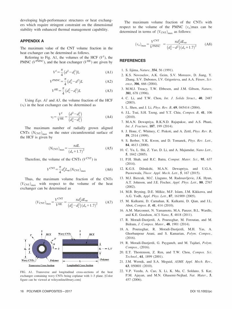
The maximum volume fraction of the CNTs with
respect to the volume of the PMNC vnð Þmax can be
determined in terms of VCNTð Þmax as follows:
vnð Þmax5VCNT
VPMNC5
pd2ndLnr
d2o2d2
� �dn11:7ð Þ2
(A8)
REFERENCES
1. S. Iijima, Nature, 354, 56 (1991).
2. K.S. Novoselov, A.K. Geim, S.V. Morozov, D. Jiang, Y.
Zhang, S.V. Dubonos, I.V. Grigorieva, and A.A. Firsov, Sci-
ence, 306, 666 (2004).
3. M.M.J. Treacy, T.W. Ebbesen, and J.M. Gibson, Nature,
381, 678 (1996).
4. C. Li, and T.W. Chou, Int. J. Solids Struct., 40, 2487
(2003).
5. L. Shen, and J. Li, Phys. Rev. B, 69, 045414 (2004).
6. J.L. Tsai, S.H. Tzeng, and Y.T. Chiu, Compos. B, 41, 106
(2010).
7. M.A.N. Dewapriya, R.K.N.D. Rajapakse, and A.S. Phani,
Int. J. Fracture, 187, 199 (2014).
8. J. Hone, C. Whitney, C. Piskoti, and A. Zettl, Phys. Rev. B,
59, 2514 (1999).
9. S. Berber, Y.K. Kwon, and D. Tomanek, Phys. Rev. Lett.,
84, 4613 (2000).
10. C. Yu, L. Shi, Z. Yao, D. Li, and A. Majumdar, Nano Lett.,
5, 1842 (2005).
11. P.H. Shah, and R.C. Batra, Comput. Mater. Sci., 95, 637
(2014).
12. K.G.S. Dilrukshi, M.A.N. Dewapriya, and U.G.A.
Puswewala, Theor. Appl. Mech. Lett., 5, 167 (2015).
13. M.J. Biercuk, M.C. Llaguno, M. Radosavljevic, J.K. Hyun,
A.T. Johnson, and J.E. Fischer, Appl. Phys. Lett., 80, 2767
(2002).
14. M.B. Bryning, D.E. Milkie, M.F. Islam, J.M. Kikkawa, and
A.G. Yodh, Appl. Phys. Lett., 87, 161909 (2005).
15. M. Kulkarni, D. Carnahan, K. Kulkarni, D. Qian, and J.L.
Abot, Compos. B, 41, 414 (2010).
16. A.M. Marconnet, N. Yamamoto, M.A. Panzer, B.L. Wardle,
and K.E. Goodson, ACS Nano, 5, 4818 (2011).
17. R. Moradi-Dastjerdi, A. Pourasghar, M. Foroutan, and M.
Bidram, J. Compos. Mater., 48, 1901 (2014).
18. A. Pourasghar, R. Moradi-Dastjerdi, M.H. Yas, A.
Ghorbanpour Arani, and S. Kamarian, Polym. Compos.,(2016).
19. R. Moradi-Dastjerdi, G. Payganeh, and M. Tajdari, Polym.
Compos., (2016).
20. E.T. Thostenson, Z. Ren, and T.W. Chou, Compos. Sci.
Technol., 61, 1899 (2001).
21. J.M. Wernik, and S.A. Meguid, ASME Appl. Mech. Rev.,63, 050801 (2010).
22. V.P. Veedu, A. Cao, X. Li, K. Ma, C. Soldano, S. Kar,
P.M. Ajayan, and M.N. Ghasemi-Nejhad, Nat. Mater., 5,
457 (2006).
FIG. A1. Transverse and longitudinal cross-sections of the heat
exchanger containing wavy CNTs being coplanar with 1–3 plane. [Color
figure can be viewed at wileyonlinelibrary.com]
16 POLYMER COMPOSITES—2017 DOI 10.1002/pc
23. E. Bekyarova, E.T. Thostenson, A. Yu, H. Kim, J. Gao, J.
Tang, H.T. Hahn, T.W. Chou, M.E. Itkis, and R.C. Haddon,
Langmuir, 23, 3970 (2007).
24. E.J. Garcia, B.L. Wardle, A.J. Hart, and N. Yamamoto,
Compos. Sci. Technol., 68, 2034 (2008).
25. K.H. Hung, W.S. Kuo, T.H. Ko, S.S. Tzeng, and C.F. Yan,
Compos. A Appl. Sci., 40, 1299 (2009).
26. D.C. Davis, J.W. Wilkerson, J.A. Zhu, and D.O.O. Ayewah,
Compos. Struct., 92, 2653 (2010).
27. J.E. Zhang, R.C. Zhuang, J.W. Liu, E. Mader, G. Heinrich,
and S.L. Gao, Carbon, 48, 2273 (2010).
28. D.C. Davis, J.W. Wilkerson, J. Zhu, and V.G. Hadjiev,
Compos. Sci. Technol., 71, 1089 (2011).
29. S.I. Kundalwal, and M.C. Ray, Acta Mech., 225, 2621 (2014).
30. S.I. Kundalwal, and S. Kumar, Mech. Mater., 102, 117
(2016).
31. S.I. Kundalwal, and S.A. Meguid, Eur. J. Mech. A Solid,
64, 69 (2017).
32. R. Rafiee, and A. Ghorbanhosseini, Int. J. Mech. Mater.Design, 12, 1 (2016).
33. R. Rafiee, and A. Ghorbanhosseini, Mech. Mater., 106, 1
(2017).
34. R. Moradi-Dastjerdi, and H. Momeni-Khabisi, Steel Com-pos. Struct., 22, 277 (2017).
35. R. Moradi-Dastjerdi, and G. Payganeh, Polym. Compos., (2017).
36. R. Moradi-Dastjerdi, and H. Momeni-Khabisi, J. Vib. Con-trol, (2017).
37. F.T. Fisher, R.D. Bradshaw, and L.C. Brinson, Compos. Sci.Technol., 63, 1689 (2003).
38. R.D. Bradshaw, F.T. Fisher, and L.C. Brinson, Compos. Sci.Technol., 63, 1705 (2003).
39. V. Anumandla, and R.F. Gibson, Compos. A, 37, 2178
(2006).
40. X. Chen, I.J. Beyerlein, and L.C. Brinson, Mech. Mater.,41, 279 (2009).
41. R. Rafiee, Compos. Struct., 97, 304 (2013).
42. T. Mori, and K. Tanaka, Acta Metall., 21, 571 (1973).
43. Y.P. Qui, and G.J. Weng, Int. J. Eng. Sci., 28, 1121 (1990).
44. N. Laws, J. Mech. Phys. Solids, 21, 9 (1973).
45. H.M. Hsiao, and I.M. Daniel, Compos. A, 27, 931 (1996).
46. H.M. Hsiao, and I.M. Daniel, Compos. Sci. Technol., 56,
581 (1996).
47. C. Tsai, C. Zhang, D.A. Jack, R. Liang, R, and B. Wang,
Compos. B, 42, 62 (2011).
48. J.Y. Li, and M.L. Dunn, Philos. Mag. A, 77, 1341 (1998).
49. J. Aboudi, S.M. Arnold, and B.A. Bednarcyk, Butterworth-
Heinemann Ltd., Oxford OX5 (2012).
50. C.W. Nan, R. Birringer, D.R. Clarke, and H. Gleiter, J.
Appl. Phys., 81, 6692 (1997).
51. A.R. Alian, S.I. Kundalwal, and S.A. Meguid, 24th Interna-
tional Congress of Theoretical and Applied Mechanics, 21–
26 August 2016, Montreal, Canada.
52. J.F. Villeneuve, R. Naslain, R. Fourmeaux, and J. Sevely,
Compos. Sci. Technol., 49, 89 (1993).
53. S.T. Peters, Handbook of Composites, Chapman and Hall,
London (1998).
54. Y.K. Kwon, S. Berber, and D. Tomanek, Phys. Rev. Lett.,
92, 015901 (2004).
55. K. Honjo, Carbon, 45, 865 (2007).
56. C.L. Zhang, and H.S. Shen, Appl. Phys. Lett., 89, 081904
(2006).
57. F. Scarpa, L. Boldrin, H.X. Peng, C.D.L. Remillat, and S.
Adhikari, Appl. Phys. Lett., 97, 151903 (2010).
58. S.I. Kundalwal, and S.A. Meguid, Eur. J. Mech. A Solid,
53, 241 (2015).
59. L.Y. Jiang, Y. Huang, H. Jiang, G. Ravichandran, H. Gao,
K.C. Hwang, and B. Liu, J. Mech. Phys. Solids, 54, 2436
(2006).
60. S.J.V. Frankland, V.M. Harik, G.M. Odegard, D.W.
Brenner, and T.S. Gates, Compos. Sci. Technol., 63, 1655
(2003).
61. S.I. Kundalwal, and M.C. Ray, Int. J. Mech. Mater. Design,
7, 149 (2011).
62. S.I. Kundalwal, and M.C. Ray, ASME J. Appl. Mech., 80,
021010 (2013).
63. D.C. Hammerand, G.D. Seidel, and D.C. Lagoudas, Mech.
Adv. Mater. Struct., 14, 277 (2007).
64. M.R. Ayatollahi, S. Shadlou, and M.M. Shokrieh, Compos.
Struct., 93, 2250 (2011).
65. J.L. Wang, M. Gu, W.G. Ma, X. Zhang, and Y. Song, New
Carbon Mater., 23, 259 (2008).
66. W. Reese, J. Appl. Phys., 37, 864 (1996).
67. O.M. Wilson, X. Hu, D.G. Cahill, and P.V. Braun, Phys.
Rev. B, 66, 224301 (2002).
DOI 10.1002/pc POLYMER COMPOSITES—2017 17


![Thermomechanical Analysis [TMA] [NETZSCH]](https://img.pdfslide.net/doc/110x75/55cf940b550346f57b9f3bd8/thermomechanical-analysis-tma-netzsch.jpg)