MODELING RAINFALL-RUNOFF RELATIONSHIPS FOR THE ANJENI

WATERSHED IN THE BLUE NILE BASIN

A Thesis

Presented to the Faculty of the Graduate School

of Cornell University

in Partial Fulfilment of the Requirements for the Degree of

Master of Professional Studies

By

Elias Sime Legesse

August 2009

© 2009 Elias Sime Legesse

ABSTRACT

Models accurately representing the underlying hydrological processes in the Nile

Basin are necessary for implementation of effective soil and water conservation

practices. Despite this, most models currently being used in the Nile basin have been

developed for temperate climates and might not apply fully to the monsoonal climates

with distinct dry periods in the Nile basin. Recently a landscape based hydrology

model was developed for the monsoonal climates in the Ethiopian highlands by

dividing the watershed in areas that produce runoff and areas in which the all water

infiltrates and eventually becomes interflow or base flow. The model was calibrated

and validated to predict the discharge of the whole Blue Nile Basin. The objective of

this study was to test the validity of the assumptions concerning the runoff processes

on a small scale. The study was carried out in the Anjeni Watershed in the Blue Nile

Basin for which discharge and rainfall measurements were available for an extended

period. Thirty piezometers were installed in four transects and the water table was

measured during the rainy season. The performance of the model was evaluated using

three different techniques: coefficient of determination, Nash and Sutcliff, and root

mean square error (RMSE). Model calibration and validation indicated a good fit

between the observed and simulated discharge values. Values of coefficient of

determination for calibration were obtained to be 0.84, 0.89 and 0.95 for the daily,

weekly and monthly time steps, respectively. Similarly, Nash and Sutcliff values of

0.84, 0.83 and 0.96 were obtained respectively. The runoff production mechanism in

the Northern part found to be saturation excess although in practice there is very little

difference with infiltration excess runoff while in the southern, a combination of

saturation excess from the top and flow of water through cracks and openings with

more percentage of the flow is through the cracks and fissures.

BIOGRAPHICAL SKETCH

Elias Sime Leggesse was born in Ethiopia, on June 4, 1980. After earning a B.Sc in

Hydraulic Engineering in 1998 from Arbaminch University, he became interested in

teaching and immediately after graduation started to teach in Bahirdar Construction

technology College, Bahirdar and taught for nearly two years. Then he joined Bahirdar

University and worked as an assistant lecturer. Because of his immense interest to

pursue his education in hydrology he joined integrated Watershed Management and

Hydrology Masters Program in 2007.

iii

ACKNOWLEDGEMENTS

First, I am very grateful for Tammo Steenhuis, Ph.D. Professor for his generosity to

open such a program in the country, which could help many students to continue their

second degree. I consider myself a very fortunate person to be a part of the program

which as a matter of fact was my priority to study.

I would like to forward my appreciation to, Dr. Amy Collick who was very close,

supportive, epigram and patient from the beginning to the end, without her it would

have been difficult to finish the study. In addition, I am thankful to my family,

classmates and friends who were with me physically and morally.

Finally, I would like to acknowledge the financial support of Bahir Dar University

and thesis support from the CGIAR Challenge Program on Water and Food (CPWF)

and the International Water Management Institute (IWMI) managed project, PN19

‘Upstream-Downstream in the Blue Nile’. I also forward my heart felt thank to

ARARI and the people who work there for providing me data and for their assistances

and comments: Ato Tadele, Mohamed, Deresse and Ato Gizaw.

iv

TABLE OF CONTENTS

BIOGRAPHICAL SKETCH.........................................................................................iii

ACKNOWLEDGEMENTS .......................................................................................... iv

TABLE OF CONTENTS ...............................................................................................v

LIST OF FIGURES......................................................................................................vii

LIST OF TABLES ........................................................................................................ ix

1 Introduction....................................................................................................1

1.1 Introduction....................................................................................................1

1.2 Hypothesis of the study .................................................................................3

2 Description of the Study Area .......................................................................4

2.1 General...........................................................................................................4

2.2 Climatic Characteristics.................................................................................4

2.3 Topography and soils.....................................................................................5

2.4 Land use/cover...............................................................................................9

2.5 Hydrology ......................................................................................................9

2.6 TManagement practices...............................................................................10

3 Methodology................................................................................................11

4 Rainfall-Runoff Modeling ...........................................................................14

4.1 Model formulation .......................................................................................14

4.2 Data Used.....................................................................................................17

5 Results..........................................................................................................20

5.1 Piezometer reading result ............................................................................20

5.2 Calibration and validation result..................................................................21

5.3 Model evaluation .........................................................................................27

6 Discussion....................................................................................................33

v

7 Conclusions and Recommendation..............................................................37

REFERENCE ...............................................................................................................39

APPENDIX ..................................................................................................................42

Appendix A Mean monthly effective precipitation..........................................42

Appendix B Mean monthly discharge..............................................................42

Appendix C Runoff coefficient ........................................................................43

Appendix D Daily rainfall runoff graph: Anjeni 1988-1997............................43

Appendix E Weekly rainfall runoff graph: Anjeni 1988-1997 ........................44

Appendix F Mean monthly rainfall runoff graph: Anjeni 1988-1977..............44

vi

LIST OF FIGURES

Figure 2-1 Contour map of Anjeni watershed................................................................6

Figure 2-2 Soil map of the Anjeni watershed ................................................................7

Figure 2-3 Soil depth map of the Anjeni watershed.......................................................8

Figure 3-1 Satellite image of land use/cover showing locations of piezometers and

gully in the Anjeni watershed ......................................................................12

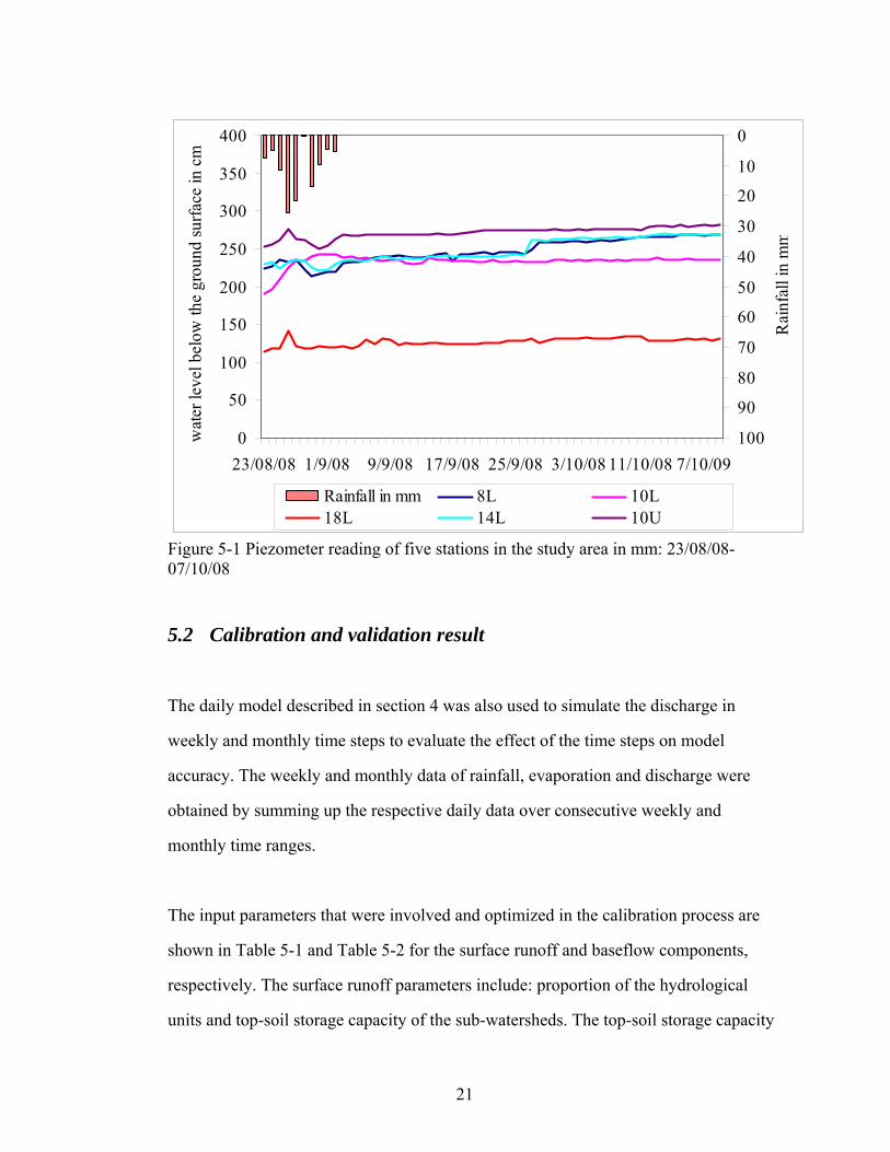
Figure 5-1 Piezometer reading of five stations in the study area in mm: 23/08/08-

07/10/08 .......................................................................................................21

Figure 5-2 Comparison of calibrated daily simulated discharge and observed

discharge: 1994............................................................................................24

Figure 5-3 Comparison of calibrated weekly simulated discharge and observed

discharge: 1988-1994...................................................................................24

Figure 5-4 Comparison of calibrated monthly simulated discharge and observed

discharge: 1988-1994...................................................................................25

Figure 5-5 Comparison of validated daily simulated discharge and observed discharge:

1997 .............................................................................................................26

Figure 5-6 Comparison of validated weekly simulated discharge and observed

discharge: 1997............................................................................................26

Figure 5-7 Comparison of validated Monthly simulated discharge and observed

discharge: 1997............................................................................................27

Figure 5-8 Graph of daily observed discharge versus simulated discharge: 1988-1994

.....................................................................................................................28

Figure 5-9 Graph of weekly observed discharge versus simulated discharge: 1988-

1994 .............................................................................................................29

vii

Figure 5-10 Graph of monthly observed discharge versus simulated discharge: 1988-

1994 .............................................................................................................29

Figure 5-11 Graph of validated daily observed discharge versus simulated discharge:

1997 .............................................................................................................30

Figure 5-12 Graph of validated weekly observed discharge versus simulated

discharge: 1997............................................................................................30

Figure 5-13 Graph of validated monthly observed discharge versus simulated

discharge: 1997............................................................................................31

Figure 6-1: Picture showing cracks and fissures of the sub-soil ..................................35

Figure 6-2: Picture showing close-up of crack in the sub-soil .....................................35

viii

LIST OF TABLES

Table 2-1 Major soil groups of Anjeni watershed..........................................................7

Table 3-1 Summary of piezometer installation ............................................................13

Table 5-1 Parameter values of the water balance model..............................................23

Table 5-2 Model parameter for the baseflow section...................................................23

Table 5-3: Summary of the result of the three model performance evaluation

techniques for calibration and validation.....................................................28

ix

1 Introduction

1.1 Introduction

The Abay-Blue Nile is the largest tributary of the Nile River; providing a vital source

of freshwater to the downstream riparian users in Sudan and Egypt. In addition, the

basin deposits sediment downstream which affects both upstream and downstream

countries of the basin. Upstream, the erosion problem is degrading the land and

reducing agricultural production while downstream the deposition of sediment is

reducing reservoir capacities and is causing increased flooding that threatens the life

of many people, structures, and property. The problem encompasses the interests of

many nations within the Nile Basin and must involve scientists from different

disciplines in the area to work together to mitigate the consequences of severe erosion

and sedimentation in the basin. Consequently, planning and implementing effective

and sustainable soil and water conservation practices has taken precedence in reducing

erosion and its effects in the Ethiopian highlands.

Design of effective soil and water conservation practices should take into account the

type of runoff generating mechanism. Conversely, the soil and water conservation

practices itself can affect the runoff processes of the watershed. Understanding the

runoff processes is therefore of paramount importance for sustainable watershed

management. However as of yet, little has been done on fully understanding the

runoff generation mechanisms, evaluating factors that affect runoff generation

mechanisms and developing conceptual models based on understanding the watershed

hydrological processes and the cause and effect of conservation practices.

1

The runoff generating mechanisms influence a broad range of processes in a

watershed, including soil erosion, biogeochemical cycling, and in-channel sediment

transport. Surface runoff generation mechanisms can be classified as either infiltration

excess or saturation excess processes (Sklash, 1990). Infiltration excess, or Hortonian

overland flow, occurs where rainfall intensities exceed the infiltration capacities of

soil. Saturation excess occurs when the water table rises to near the surface and

saturate the profile and thereby minimizing infiltration rate.

The main objective of this study is to better understand the hydrology of the Blue Nile

Basin. The particular objectives are (1) identification of the dominant types of runoff

mechanisms in the study area, (2) determination of the most important factors that

influence these mechanisms, and (3) testing of a simplified water balance model that

incorporated the influential runoff mechanisms to determine the rainfall runoff

relationship and estimate streamflow.

The study was carried out in the Anjeni Watershed, a small watershed located within

the Blue Nile basin. The topographical setting and climate of the Anjeni watershed is

representation for most of the upstream part of the Blue Nile Basin and because of its

long record of discharge, erosion and rainfall measurements makes it is an important

for the study of hydrology, climate change, agriculture and meteorology. In addition

to these measurements, piezometers were installed to measure (perched) ground water

table heights. The data were used for calibration and validation of the model with a

daily, weekly, and monthly time steps.

The study has a practical implication in providing insights into the determination of

runoff generating mechanisms, which in turn has practical implications in the selection

2

of appropriate soil and water conservation practices, a major concern at regional and

basin scales.

1.2 Hypothesis of the study

The hypotheses of the research are described below:

1. Runoff processes are mainly affected by topography, soil type and soil depth.

2. Planning and implementation of soil and water conservation requires

consideration of different types of runoff generating mechanisms of the area.

3. Reliable information can be derived from a simple water balance hydrologic

model.

3

2 Description of the Study Area

2.1 General

The watershed area of Anjeni is in the Gojam Zone (northwest Ethiopia) on a river

originating from the Choke Mountains (4154 meters above sea level (masl)). Anjeni is

approximately 13 km northeast of the nearest town, Dembecha. The total area of the

catchment is 113.4 ha with elevations ranging between 2405 and 2500 masl. The area

is intensively cultivated. Anjeni was one of the Soil Conservations Research Units

(SCRP) where extensive records of hydrological data were collected, including

precipitation (P), potential evapotranspiration (PET), and discharge (Q) for about 20

years from 1988-2008.

2.2 Climatic Characteristics

In this watershed, annual rainfall mostly occurred between May and October in a

unimodal distribution. The major rainfall during the rainy season, between June and

September, accounted for 75% of the total annual rainfall. The average annual values

of temperature, precipitation, potential evapotranspiration and discharge in the

watershed were 12.6oC, 1,480 mm, 1,160 mm and 723 mm, respectively.

The overland flow of the catchment drains from northeast (NE) to southwest (SW)

into the perennial Minchet River with a mean annual discharge of about 730 mm

(1985-1993) and a low coefficient of variation of 10%.

4

5

2.3 Topography and soils

The watershed has almost a rectangular shape and north-south (NS) orientation with

the Minchet River dissecting the watershed through the middle. It is in the slope

category from 8 to 30% according to the Food and Agriculture Organization (FAO)

slope classification and is flanked on three sides by plateau (see Figure 2-1). The

middle can be described as having a convex shape.

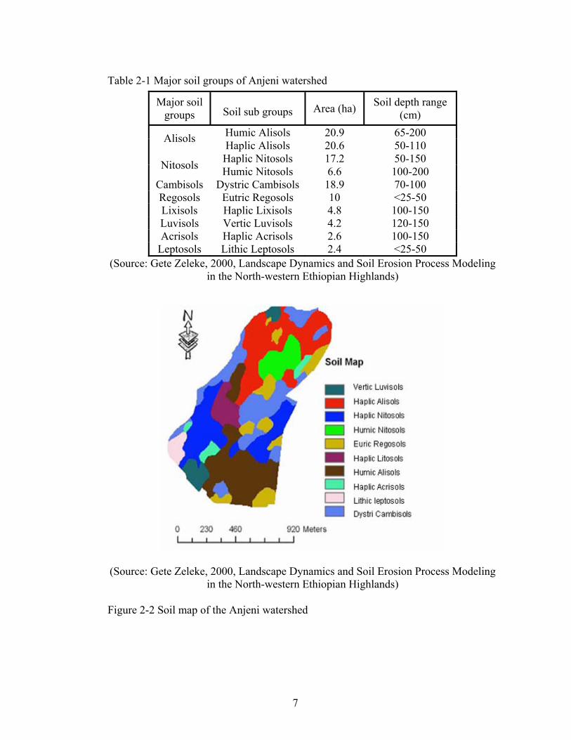
The soils of Anjeni have developed on the basalt and volcanic ash of the plateau. More

than 90% of the watershed area consists of four types of soils. The southern valley

bottoms and concave parts of the catchment are predominantly covered with deep,

well weathered humic alisols (21%), while the shallower Haplic Alisols (21%)

covered most of the northern part of the watershed (see Figure 2-1). Moderately deep

red Nitosols (found on 24% of the catchment); Haplic Nitosols (17%) distributed

mostly in the south western gently sloping part and some in the east steep upper slopes

and Humic Nitosols (6.6%) covered in the central northern watershed. Regosols and

Leptosols (12%) scattered in the northern steep slopes, mainly convex in shape and in

southern boundaries of the watershed with very shallow depth. The middle area

covered with moderately deep, young Dystric Cambisols (19%). Other soils like

Luvisols, Leptosols and Acrisols are also found in small pockets in the catchment (see

Table 2-1and Figure 2-2).

(Source: cartography and photogrammetry Max Zurbuchen, institute of photogrammetry and Engineering Survey, Bern,

Switzerland (adapted from SCRP, Ethiopia, Database report (1984-1993, Anjeni Research Unit, research report 37))

6

Figure 2-1 Contour map of Anjeni watershed

7

Table 2-1 Major soil groups of Anjeni watershed

(Source: Gete Zeleke, 2000, Landscape Dynamics and Soil Erosion Process Modeling in the North-western Ethiopian Highlands)

(Source: Gete Zeleke, 2000, Landscape Dynamics and Soil Erosion Process Modeling

in the North-western Ethiopian Highlands) Figure 2-2 Soil map of the Anjeni watershed

Major soil groups

Soil sub groups Area (ha) Soil depth range

(cm) Humic Alisols 20.9 65-200 Alisols Haplic Alisols 20.6 50-110 Haplic Nitosols 17.2 50-150 Nitosols Humic Nitosols 6.6 100-200

Cambisols Dystric Cambisols 18.9 70-100 Regosols Eutric Regosols 10 <25-50 Lixisols Haplic Lixisols 4.8 100-150 Luvisols Vertic Luvisols 4.2 120-150 Acrisols Haplic Acrisols 2.6 100-150

Leptosols Lithic Leptosols 2.4 <25-50

8

(Source: SCRP, Ethiopia, Database report (1984-1993), series V: Anjeni Research Unit, University of Bern, Switzerland in association with the ministry of agriculture, Ethiopia.) Figure 2-3 Soil depth map of the Anjeni watershed

2.4 Land use/cover

About 70% of the watershed was cultivated between the years 1984-1991. Currently

more than 90% of the watershed is used for agricultural production, mostly teff, maize,

wheat, barley, and nug (Niger seed) with beans, linseed, gibbto (lupine species used

for traditional alcohol, areky, production) being planted at a lesser extent. The land

around the river edge is uncultivated and covered with grass. Barely is planted twice

(July and September). Teff and wheat are seeded late in the summer, after August 20,

or after the heavy rainfall period has passed. Crop land preparation involved the

plowing more than two to three times of the soil in the heavy storm period. This means

the croplands are bare during most of the heavy rainy period, and high soil erosion has

been recorded by the measurement of rills observed on the surface of the cropland.

2.5 Hydrology

Mean monthly effective precipitation and mean monthly discharge are shown in

Appendix A and Appendix B, and the relationship of rainfall to discharge for daily,

weekly and monthly time steps are depicted in Appendix D, Appendix E, and

Appendix F. Rainfall (from one gauging station (pluviometer) in the watershed) and

discharge measurements were recorded. The annual rainfall occurred mainly between

May and October in a unimodal distribution. The majority of annual rainfall falls

between June and September during the main rainy season accounting for 75% of the

total annual rainfall and the peak rainfall occurs commonly during July. On the other

hand, the peak monthly average runoff occurs in August. The runoff coefficient value

is high in the watershed in the month of August for the rainfall periods from May to

September as indicated in Appendix C.

9

2.6 Management practices

Before 1985 there were no management activities in the Anjeni watershed. Fanya juus

(SWC structure comprised of a bund in the upper part and a drainage ditch in the

lower part) were then constructed in 1986 throughout the watershed. The decrease in

annual suspended sediment load by the construction of fanya juus between 1986 and

1989 as compared to the prior year were reported. Later between 1990 and 1993 the

annual suspended sediment load has risen to pre-1986 due to poor maintenance

(Bossart 1995; Ludi 1994). The effect of terracing can be seen by the difference in

elevation made by the deposited soil in two consecutive fields in a down-slope

direction.

10

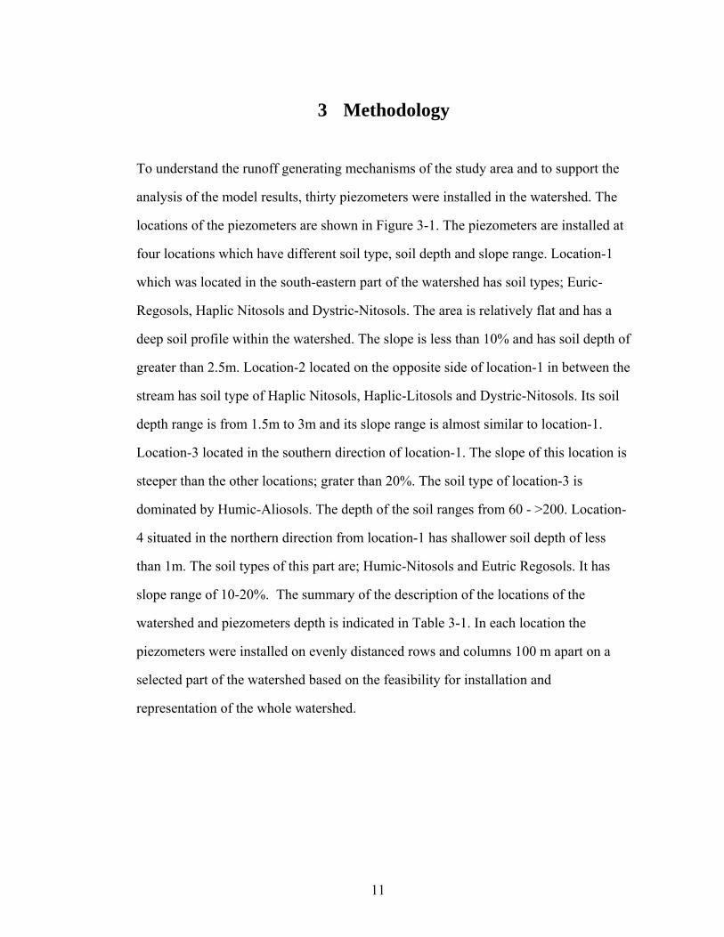
3 Methodology

To understand the runoff generating mechanisms of the study area and to support the

analysis of the model results, thirty piezometers were installed in the watershed. The

locations of the piezometers are shown in Figure 3-1. The piezometers are installed at

four locations which have different soil type, soil depth and slope range. Location-1

which was located in the south-eastern part of the watershed has soil types; Euric-

Regosols, Haplic Nitosols and Dystric-Nitosols. The area is relatively flat and has a

deep soil profile within the watershed. The slope is less than 10% and has soil depth of

greater than 2.5m. Location-2 located on the opposite side of location-1 in between the

stream has soil type of Haplic Nitosols, Haplic-Litosols and Dystric-Nitosols. Its soil

depth range is from 1.5m to 3m and its slope range is almost similar to location-1.

Location-3 located in the southern direction of location-1. The slope of this location is

steeper than the other locations; grater than 20%. The soil type of location-3 is

dominated by Humic-Aliosols. The depth of the soil ranges from 60 - >200. Location-

4 situated in the northern direction from location-1 has shallower soil depth of less

than 1m. The soil types of this part are; Humic-Nitosols and Eutric Regosols. It has

slope range of 10-20%. The summary of the description of the locations of the

watershed and piezometers depth is indicated in Table 3-1. In each location the

piezometers were installed on evenly distanced rows and columns 100 m apart on a

selected part of the watershed based on the feasibility for installation and

representation of the whole watershed.

11

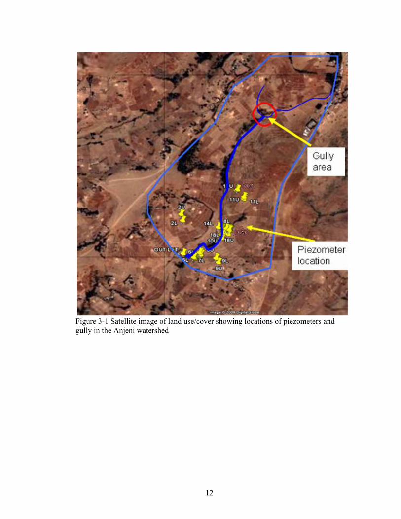
Figure 3-1 Satellite image of land use/cover showing locations of piezometers and gully in the Anjeni watershed

12

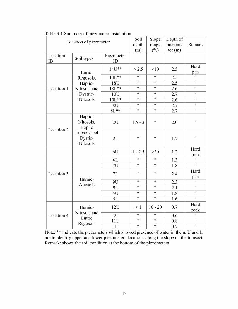
Table 3-1 Summary of piezometer installation

Location of piezometer

Soil depth (m)

Slope range (%)

Depth of piezometer (m)

Remark

Location ID Soil types Piezometer

ID

14U** > 2.5 <10 2.5 Hard pan

14L** “ “ 2.5 “ 18U “ “ 2.5 “

18L** “ “ 2.6 “ 10U “ “ 2.7 “

10L** “ “ 2.6 “ 8U “ “ 2.7 “

Location 1

Euric-Regosols, Haplic-

Nitosols and Dystric-Nitosols

8L** “ “ 2.7 “

2U 1.5 - 3 “ 2.0 “ Location 2

Haplic-Nitosols, Haplic

Litosols and Dystic-Nitosols

2L “ “ 1.7 “

6U 1 - 2.5 >20 1.2 Hard rock

6L “ “ 1.3 “ 7U “ “ 1.8 “

7L “ “ 2.4 Hard pan

9U “ “ 2.3 “ 9L “ “ 2.1 “ 5U “ “ 1.8 “

Location 3

Humic-Aliosols

5L “ “ 1.6 “

12U < 1 10 - 20 0.7 Hard rock

12L “ “ 0.6 “ 11U “ “ 0.8 “

Location 4

Humic-Nitosols and

Eutric Regosols

11L “ “ 0.7 “ Note: ** indicate the piezometers which showed presence of water in them. U and L are to identify upper and lower piezometers locations along the slope on the transect Remark: shows the soil condition at the bottom of the piezometers

13

4 Rainfall-Runoff Modeling 4.1 Model formulation

A simple water balance model was developed and tested by Collick et al (2008) to

predict the stream flow for four relatively small watersheds (< 500 ha) in the Blue Nile

(Abay, Ethiopian name) Basin, including the Anjeni watershed. The author reported

reasonable predictions on a daily and weekly time step using nearly identical

parameters for watersheds of hundreds kilometers apart. In this study, some minor

modifications were made with respect to interflow generation for predicting discharge

of the Anjeni watershed. A detailed description of the water balance model follows

(Steenhuis et al., 2009).

In the model, the watershed is considered to be composed of two areas. One portion is

the upland area (upper portion of the watershed) producing direct runoff with little

interflow and base flow. The second portion is the bottomland (middle lower portion

of the watershed) producing base flow with little interflow and direct runoff. As it is

described the upland portion is characterized by shallow soil depth with weathered and

outcropped rock in some parts and steep slope. While the saturation portion of the

watershed is deep soil and relatively mild slope. The classifications were made based

on the soil depth map, soil type map, and the effect of management activity.

The amount of water stored in the top most layer (root zone) of the soil S (mm), for

the upland and bottomland were estimated separately using the modification of the

Thornthwaite-Mather water balance equation in Collick et al (2008).

( ) tPAETPSS erctt Δ−−+= Δ− (1)

14

Where S (mm) is moisture storage, St-Δt (mm) previous time step storage, R (mm/day)

runoff, AET (mm) the actual evapotranspiration, Perc (mm/day) is percolation.

During wet periods when the rainfall exceeds evapotranspiration (i.e., P > PET), the

actual evapotranspiration, AET, is equal to the potential evapotranspiration, PET.

Conversely, when evaporation exceeds rainfall (i.e., P < PET), the Thornthwaite and

Mather (1955) procedure is used to calculate evapotranspiration, AET (Steenhuis and

Van der Molen, 1986). In this method AET decreases linearly with moisture content.

(2) ⎟⎟⎠

⎞⎜⎜⎝

⎛=

maxSSPETAET t

The available soil storage capacity, Smax (mm) is defined as the difference between the

amount of water stored in the top soil layer at wilting point and the maximum moisture

content, equal to either the field capacity for the hillslope soils or saturation (e.g., soil

porosity) in runoff contributing areas. Smax varies according to soil characteristics

(e.g., porosity and bulk density) and soil layer depth. Based on Equation 2 the surface

soil layer moisture storage can be written as:

( )

⎥⎦

⎤⎢⎣

⎡⎟⎟⎠

⎞⎜⎜⎝

⎛ Δ−= Δ−

max

expS

tPETPSS ttt When P<PET (3)

In this simplified model direct runoff occurs from both the runoff contributing area

and the saturation area when the soil moisture balance indicates that the soil is

saturated. Base flow and interflow originate only from the saturation area. It is

assumed that the surface runoff from these areas is minimal. This will underestimate

the runoff during major rainfall events but since our interest is in weekly to monthly

intervals was not considered a major limitation.

15

In the overland flow contributing area when rainfall exceeds evapotranspiration and

fully saturates the soil, any moisture above saturation becomes runoff, and the runoff,

R, can be determined by adding the change in soil moisture from the previous time

step to the difference between precipitation and actual evapotranspiration.

tPETPSR tt Δ−+= Δ− )( (4a)

maxSSt = (4b)

For saturation area, the excess rainfall (ER) is calculated in the same way as the

overland flow in the overland flow contributing area. However, the excess rainfall(ER)

is considered to be composed of direct runoff and interflow or base flow. The direct

runoff is separated from the interflow or base flow by subtracting the rainfall in excess

of the saturation area multiplied by recharge factor form the excess water. The

remaining part (the saturation excess multiplied by recharge factor) of the water flows

as interflow or base flow to the stream.

tPETPSER tt Δ−+= Δ− )( (5a)

maxSSt = (5b)

The sum of the interflow and the base flow routed to two reservoirs that produce base

flow and interflow. We assumed that the base flow reservoir is filled first and when

full, the interflow reservoir starts filling. The base flow reservoir acts as a linear

reservoir and its outflow, BF, and storage, BSt, are calculated when storage is less

than the maximum storage, BSmax as:

( ) tBFPRSRS ttercttt Δ−+= Δ−Δ− (6a)

⎥⎦⎤

⎢⎣⎡

ΔΔ−−

=t

taRSBF tt)exp(1

(6b)

16

Where RSt (mm/day) is the base flow reservoir, RSt-Δt is the previous time step base

flow storage, BFt-Δt is the previous time step flow, BFt is the base flow, α (1/day) is the

recession coefficient and Δt is the time step that is day.

The runoff from each sub-watershed is the sum the direct runoff and the base flow.

When the maximum storage, BSmax is reached then:

maxBSBSt = (7a)

∗≤ ττ

⎥⎦⎤

⎢⎣⎡

ΔΔ−−

=t

tRSBS tt)exp(1 α (7b)

The interflow part of the flow is considered to decreases linearly (i.e., a zero order

reservoir) after a recharge event. The total interflow, IFt at time t can be obtained by

superimposing the fluxes for the individual events:

,122,1,0

⎟⎠⎞

⎜⎝⎛ − ∗∗

=

∗−∑

∗

ττ

τ

τ

ττtPercIF (8)

Where , is the duration of the period after the rainstorm until the interflow ceases,

is the interflow at a time t, is the percolation on

∗τ

tIF ∗−τtPerc τ−t days.

4.2 Data Used

The data for Anjeni were obtained from the Amhara Region Agricultural Research

Institute (ARARI) research center at Adet (SCRP data base) and from other literature

conducted in the area. The precipitation, evaporation and discharge data record

includes 20 years from 1988-2008. Some data were not available for the years

between 2000 and 2008. The quality of the data for the years 1998 and 1999 were also

17

poor; there was no significant amount of discharge even though there was a significant

amount of precipitation data. Due to missing data and poor quality, the model

calibration was limited to six years of data for calibration; ranging from 1988-1994,

one year’s data for validation; 1997. The event-based precipitation and discharge data

were transformed to daily, weekly and monthly precipitation data in mm. The

evaporation data were also preprocessed to daily, weekly and monthly values in mm.

The weekly and monthly data were obtained by summing up the daily data over the

week and month periods, respectively.

The performance of the water balance model during calibration was evaluated by three

different techniques: coefficient of determination, Nash and Sutcliff efficiency index

and root mean square error (RMSE).

Traditionally, the coefficient of determination and standard error of estimate have

been used to measure the goodness of fit of the calibration. The coefficient of

determination assumes that the model being tested is unbiased. , i.e., the sum of the

errors is equal to zero (McCuen et al. 1990). Graphs were drawn using observed

discharge versus simulated discharge for each time step to see how well the two

curves fit each other.

Nash and Sutcliff (1970) proposed an alternative goodness-of-fit index, which is often

referred to as the efficiency index (Ef) expressed mathematically in equation (9).

(9)

( )

( ) ⎟⎟⎟⎟

⎠

⎞

⎜⎜⎜⎜

⎝

⎛

−

−−=

∑

∑

=

=N

iobsiobs

N

iisimiobs

QQ

QQEI

1

2,

1

2,,

1

18

Where Qobs is the observed discharge, Qsim is the simulated discharge.

The efficiency index or Nash-Sutcliff criterion is often used to measure the

performance of a hydrological model. The efficiency index lies in the interval from -∞

to +1. For biased models, the efficiency index may actually be algebraically negative.

The zero value means the model performs equal to a naïve predication, that is, a

prediction using an average observed value. A value between 0.6-0.8 is a moderate to

good fit. A value of more than 0.8 is a good fit. A value of one is a perfect fit.

2/12

,, )(

⎟⎟⎟⎟

⎠

⎞

⎜⎜⎜⎜

⎝

⎛−

=∑

N

QQRMSE

N

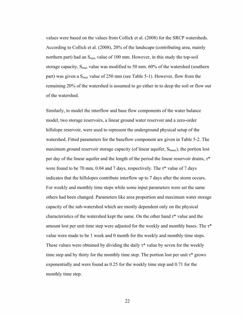
iisimiobs (10)

The root mean square error defined by Equation (10) measures the average error

between the observed and the simulated discharges, where Qobs is the observed

discharge, Qobs and Qsim are as described above and N is the number of observations.

The closer the RMSE value is to zero, the better the performance of the model. The

RMSE was used to measure the agreement between the observed and simulated water

balance.

19

5 Results 5.1 Piezometer reading result

The results of the piezometers readings and rainfall are illustrated in the Figure 5-1.

Rainfall records coinciding with the piezometer readings were found only for the

periods from 23/08/08 - 01/09/08 while the piezometer reading time was 23/08/08-

07/10/08. Out of the 30 piezometers around 8 were broken immediately. Out of the

rest only five piezometers have showed presence of water. All of these five

piezometers were located in location-1; in the southern part of the watershed within

10m distance from the river. These piezometers are 10L, 18L, 8L, 14L and 10U (see

Figure 3-1. The water table was found at around 1 m from the ground surface in

piezometer 18L and generally beyond 2 m for the rest of the piezometers. Initially the

piezometers responded significantly following the installation of the piezometers and

high rainfall events on 26/08/08 and 27/08/08 (Figure 4.1), then no significant

responses were seen except a gradual drawdown of the watertable. The Anjeni does

not have a perched watertable over a shallow restrictive layer such as in Maybar

(Haimanote, 2009) and Andit Tid (Tegenu, 2009), but a permanent watertable at

considerable depths in different locations and rising closer to the surface near the

stream. In the gully, there was water seeping in lower part of the 15 m deep gully,

indicating a water table at that depth.

20

0

50

100

150

200

250

300

350

400

23/08/08 1/9/08 9/9/08 17/9/08 25/9/08 3/10/08 11/10/08 7/10/09

wat

er le

vel b

elow

the

grou

nd su

rface

in c

m

0

10

20

30

40

50

60

70

80

90

100

Rai

nfal

l in

mm

Rainfall in mm 8L 10L18L 14L 10U

Figure 5-1 Piezometer reading of five stations in the study area in mm: 23/08/08-07/10/08

5.2 Calibration and validation result

The daily model described in section 4 was also used to simulate the discharge in

weekly and monthly time steps to evaluate the effect of the time steps on model

accuracy. The weekly and monthly data of rainfall, evaporation and discharge were

obtained by summing up the respective daily data over consecutive weekly and

monthly time ranges.

The input parameters that were involved and optimized in the calibration process are

shown in Table 5-1 and Table 5-2 for the surface runoff and baseflow components,

respectively. The surface runoff parameters include: proportion of the hydrological

units and top-soil storage capacity of the sub-watersheds. The top-soil storage capacity

21

values were based on the values from Collick et al. (2008) for the SRCP watersheds.

According to Collick et al. (2008), 20% of the landscape (contributing area, mainly

northern part) had an Smax value of 100 mm. However, in this study the top-soil

storage capacity, Smax value was modified to 50 mm. 60% of the watershed (southern

part) was given a Smax value of 250 mm (see Table 5-1). However, flow from the

remaining 20% of the watershed is assumed to go either in to deep the soil or flow out

of the watershed.

Similarly, to model the interflow and base flow components of the water balance

model, two storage reservoirs, a linear ground water reservoir and a zero-order

hillslope reservoir, were used to represent the underground physical setup of the

watershed. Fitted parameters for the baseflow component are given in Table 5-2. The

maximum ground reservoir storage capacity (of linear aquifer, Sbmax), the portion lost

per day of the linear aquifer and the length of the period the linear reservoir drains, τ*

were found to be 70 mm, 0.04 and 7 days, respectively. The τ* value of 7 days

indicates that the hillslopes contribute interflow up to 7 days after the storm occurs.

For weekly and monthly time steps while some input parameters were set the same

others had been changed. Parameters like area proportion and maximum water storage

capacity of the sub-watershed which are mostly dependent only on the physical

characteristics of the watershed kept the same. On the other hand τ* value and the

amount lost per unit time step were adjusted for the weekly and monthly bases. The τ*

value were made to be 1 week and 0 month for the weekly and monthly time steps.

These values were obtained by dividing the daily τ* value by seven for the weekly

time step and by thirty for the monthly time step. The portion lost per unit τ* grows

exponentially and were found as 0.25 for the weekly time step and 0.71 for the

monthly time step.

22

Table 5-1 Parameter values of the water balance model

Portion of the watershed

Storage, Smax (mm) Type of Contributing Area

0.2 50 Direct runoff contributing area

0.6 250 Interflow and Base flow contributing area

Table 5-2 Model parameter for the baseflow section

Parameters

Daily

Weekly

Monthly

Portion lost per unit of τ* 0.04 0.25 0.71 Linear aquifer Maximum water capacity,

SBmax (mm)

70

70

70 Zero order The length of time the

watershed drains after rainfall occurs, τ *

7 days

1 week

0 month

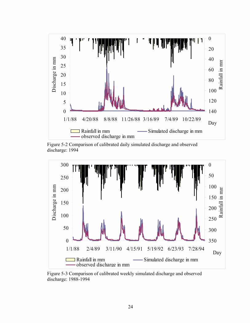
The predicted and observed discharges for all time steps with the calibrated

parameters in Tables 5.1 and 5.2 are shown in Figure 5-2, Figure 5-3, and Figure 5-4

for convenience the daily time step graph is drawn only for two years; 1988 and 1989.

The summary of the model evaluation parameters are shown in Table 5-3. Despite the

simplicity of the model, the trend between simulated and observed discharge for all

three time steps was represented well. The model has a slight tendency to overestimate

the extreme flows in all time steps but it has well represented the baseflow in the daily

and weekly time steps. Unlike the daily and weekly time steps, the model in the

monthly time step best fit the observed discharge despite its underestimation of the

baseflow. The reason is that the model with a monthly time step cannot predict the

dynamics of the saturated area well because the runoff is on the same order as the

storage.

23

0

5

10

15

20

25

30

35

40

1/1/88 4/20/88 8/8/88 11/26/88 3/16/89 7/4/89 10/22/89Day

Disc

harg

e in

mm

0

20

40

60

80

100

120

140

Rai

nfal

l in

mm

Rainfall in mm Simulated discharge in mmobserved discharge in mm

Figure 5-2 Comparison of calibrated daily simulated discharge and observed discharge: 1994

0

50

100

150

200

250

300

1/1/88 2/4/89 3/11/90 4/15/91 5/19/92 6/23/93 7/28/94Day

Disc

harg

e in

mm

0

50

100

150

200

250

300

350

Rai

nfal

l in

mm

Rainfall in mm Simulated discharge in mmobserved discharge in mm

Figure 5-3 Comparison of calibrated weekly simulated discharge and observed discharge: 1988-1994

24

0100200300400500600700800

Jan-88

Nov-88

Sep-89

Jul-90

May-91

Mar-92

Jan-93

Nov-93

Sep-94 Day

Disc

harg

e in

mm

0

200

400

600

800

1000

1200

Rai

nfal

l in

mm

Rainfall in mm Observed discharge in mmSimulated discharge in mm

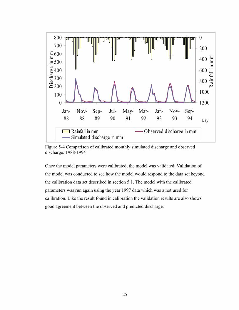
Figure 5-4 Comparison of calibrated monthly simulated discharge and observed discharge: 1988-1994

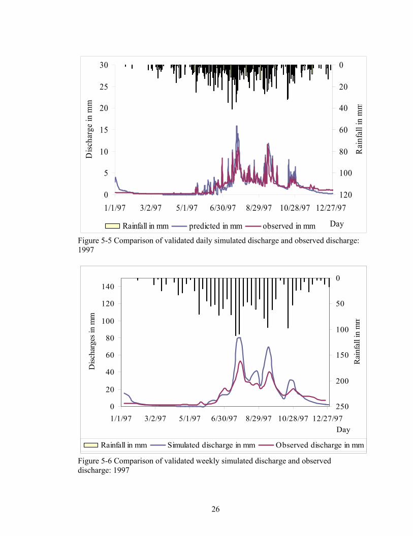
Once the model parameters were calibrated, the model was validated. Validation of

the model was conducted to see how the model would respond to the data set beyond

the calibration data set described in section 5.1. The model with the calibrated

parameters was run again using the year 1997 data which was a not used for

calibration. Like the result found in calibration the validation results are also shows

good agreement between the observed and predicted discharge.

25

0

5

10

15

20

25

30

1/1/97 3/2/97 5/1/97 6/30/97 8/29/97 10/28/97 12/27/97

Day

Disc

harg

e in

mm

0

20

40

60

80

100

120

Rai

nfal

l in

mm

Rainfall in mm predicted in mm observed in mm

Figure 5-5 Comparison of validated daily simulated discharge and observed discharge: 1997

0

20

40

60

80

100

120

140

1/1/97 3/2/97 5/1/97 6/30/97 8/29/97 10/28/97 12/27/97Day

Disc

harg

es in

mm

0

50

100

150

200

250

Rai

nfal

l in

mm

Rainfall in mm Simulated discharge in mm Observed discharge in mm

Figure 5-6 Comparison of validated weekly simulated discharge and observed discharge: 1997

26

050

100150200250300350400450500

Dec-96 Feb-97 Apr-97 Jun-97 Sep-97 Nov-97 Jan-98Day

Disc

harg

e in

mm

0

100

200

300

400

500

600

700

800

Rai

nfal

l in

mm

Rainfall in mm Observed discharge in mm Simulated discharge in mm

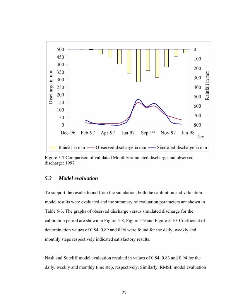
Figure 5-7 Comparison of validated Monthly simulated discharge and observed discharge: 1997

5.3 Model evaluation

To support the results found from the simulation, both the calibration and validation

model results were evaluated and the summary of evaluation parameters are shown in

Table 5-3. The graphs of observed discharge versus simulated discharge for the

calibration period are shown in Figure 5-8, Figure 5-9 and Figure 5-10. Coefficient of

determination values of 0.84, 0.89 and 0.96 were found for the daily, weekly and

monthly steps respectively indicated satisfactory results.

Nash and Sutcliff model evaluation resulted in values of 0.84, 0.83 and 0.94 for the

daily, weekly and monthly time step, respectively. Similarly, RMSE model evaluation

27

resulted in RMSE values of 1.3, 10.42 and 17.90 in mm for the three time steps,

respectively.

Table 5-3: Summary of the result of the three model performance evaluation techniques for calibration and validation

Time step Coefficient of determination

(R2)

Nash and Sutcliff

RMSE (mm)

Calibration Daily 0.84 0.84 1.3

Weekly 0.89 0.83 10.42 Monthly 0.96 0.94 17.9

Validation Daily 0.81 0.81 1.17

Weekly 0.87 0.89 9.81 Monthly 0.93 0.93 17.07

y = 1.03x - 0.10R2 = 0.84

05

101520253035

0 10 20 30 4Observed discharge in mm

Sim

ulat

ed d

ischa

rge

in m

m

0

Figure 5-8 Graph of daily observed discharge versus simulated discharge: 1988-1994

28

y = 1.32x - 2.36R2 = 0.89

-200

20406080

100120140160

0 50 100 150Observed discharge in mm

Sim

ulat

ed d

ischa

rge

in m

m

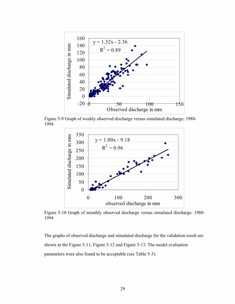
Figure 5-9 Graph of weekly observed discharge versus simulated discharge: 1988-1994

y = 1.00x - 9.18R2 = 0.96

050

100150200250300350

0 100 200 300observed discharge in mm

Sim

ulat

ed d

ischa

rge

in m

m

Figure 5-10 Graph of monthly observed discharge versus simulated discharge: 1988-1994

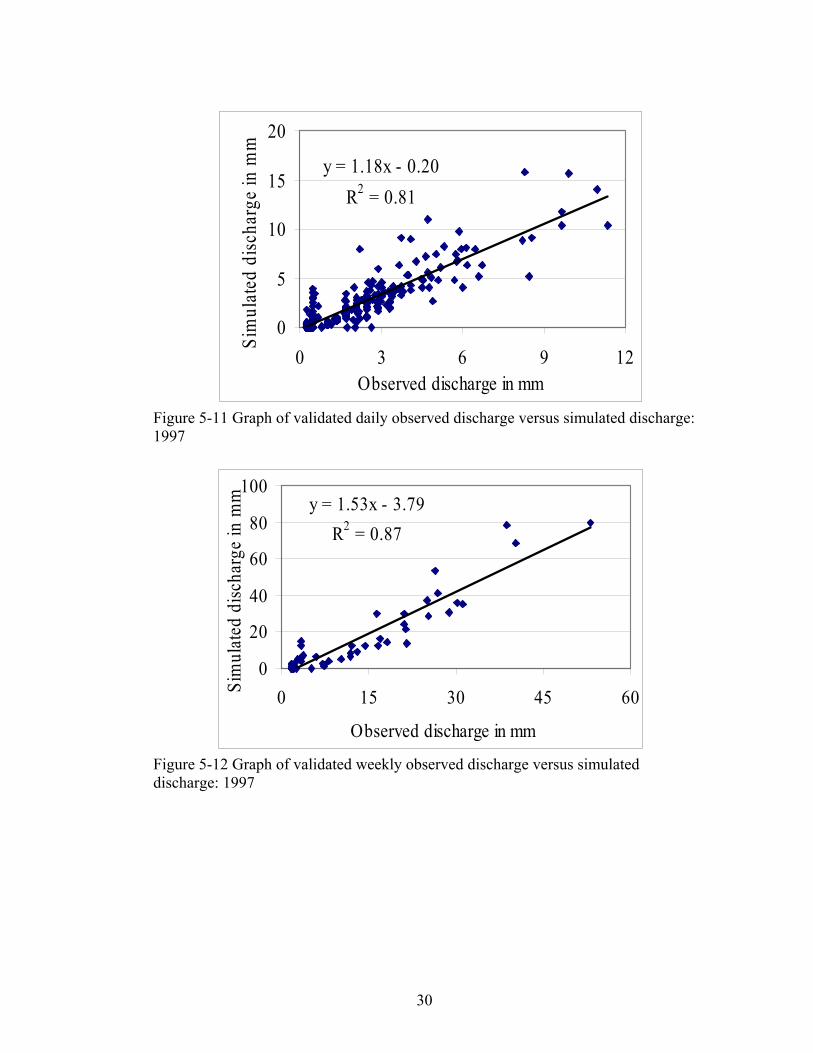
The graphs of observed discharge and simulated discharge for the validation result are

shown in the Figure 5-11, Figure 5-12 and Figure 5-13. The model evaluation

parameters were also found to be acceptable (see Table 5-3).

29

y = 1.18x - 0.20R2 = 0.81

0

5

10

15

20

0 3 6 9Observed discharge in mm

Sim

ulat

ed d

ischa

rge

in m

m

12

Figure 5-11 Graph of validated daily observed discharge versus simulated discharge: 1997

y = 1.53x - 3.79R2 = 0.87

0

20

40

60

80

100

0 15 30 45 6

Observed discharge in mm

Sim

ulat

ed d

ischa

rge

in m

m

0

Figure 5-12 Graph of validated weekly observed discharge versus simulated discharge: 1997

30

y = 1.16x - 11.53R2 = 0.93

0

50

100

150

200

0 50 100 150 200Observed discharge in mm

Sim

ulat

ed d

ischa

rge

in m

m

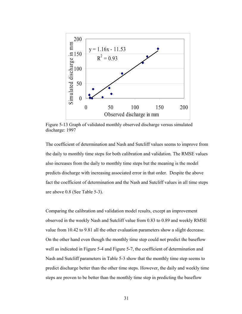
Figure 5-13 Graph of validated monthly observed discharge versus simulated discharge: 1997

The coefficient of determination and Nash and Sutcliff values seems to improve from

the daily to monthly time steps for both calibration and validation. The RMSE values

also increases from the daily to monthly time steps but the meaning is the model

predicts discharge with increasing associated error in that order. Despite the above

fact the coefficient of determination and the Nash and Sutcliff values in all time steps

are above 0.8 (See Table 5-3).

Comparing the calibration and validation model results, except an improvement

observed in the weekly Nash and Sutcliff value from 0.83 to 0.89 and weekly RMSE

value from 10.42 to 9.81 all the other evaluation parameters show a slight decrease.

On the other hand even though the monthly time step could not predict the baseflow

well as indicated in Figure 5-4 and Figure 5-7, the coefficient of determination and

Nash and Sutcliff parameters in Table 5-3 show that the monthly time step seems to

predict discharge better than the other time steps. However, the daily and weekly time

steps are proven to be better than the monthly time step in predicting the baseflow

31

discharge (see Figure 5-2 and Figure 5-3) as the RMSE values (associated error in

predicting the discharge) of the daily and the weekly time step are smaller than the

monthly time step model calibration. As higher RMSE value means high associated

error in prediction and vice versa as described above. Next to the daily, the weekly

time step has the next smallest associated error. In general it can be said that the

model could predict discharge well in all the three time steps.

32

6 Discussion

Daily, weekly, and monthly rainfall-discharge graphs are depicted in Figure 5-2,

Figure 5-3 and Figure 5-4, and the hydrographs respond quickly to rainfall. At the

same time there is a significant baseflow signal. In order to understand the hydrologic

behavior of the watershed, both topography and soils should be considered. The

topography is the main driving force for the magnitude of the flux and the soil type for

the flow path that the rain water follows.

The watershed is uniformly steep (as indicated by the equal spacing of the elevation

contour lines in Figure 2.1) unlike many other watersheds that flatten out near the

river. These flat areas near the river usually saturate in the Ethiopia highlands during

the rainy season with annual precipitation over 1000 mm. However, in the Anjeni

watershed where both the soils are deep (and the stream cuts into the soil) and there

are no flat areas all the water that otherwise would have saturated the soil drains

directly in the stream. This is confirmed by the piezometric readings. The only part in

the watershed where we found a water table was in the southern part and close to the

river only within a distance of 5 to 10m. The water table within the piezometers was

below 1 m for one piezometer and below 2.0m for the rest four piezometers (see Table

3-1 and Figure 5-1). Surprising is that the water table seems to respond throughout the

dry season. It would indicate a continuous (small) downward flow in the unsaturated

soil deep profile. Our measurement are not of long enough duration to understand if

the response would continue during the extended dry part of the year and only would

decrease during years with little rainfall.

33

The Anjeni watershed, therefore, represent a separate class of watersheds that do not

generate the runoff in the bottom saturated part of the watershed. So the overland

runoff in this watershed is generated elsewhere and is therefore dependent on the soil

type and depth and not on topography.

In Figure 2-2 the major soils types are listed. They can be separated in the deep and

highly conductive soils consisting of the Humic Alisols and Haplic Nitosols (see

Figure 2-3). These are mainly located in the southern part of the watershed. It is likely

that for these soils with extensive terracing, the water will infiltrate and flow via the

subsurface to the stream. Another clear indication that these soils are well drained is

that there were no shallow cultural ditches often implemented on the fields by farmers

in order to facilitate drainage and prevent erosion.

The soils in the northern part of the watershed are composed of mainly the shallower

Haplic Alisols and smaller proportions of Humic Nitosols and Dystric Cambisols.

These soils are shallow and have a low conductivity. On these soils despite the

terracing, farmers use the cultural ditches to channel runoff so that flows along the

contour minimize erosion. These soils are therefore likely the source of the surface

runoff as designated by the model.

In the photos in Figure 6-1 and Figure 6-2, the crack patterns observed in the southern

part during the dry season consist of mainly Humic Alisols and indicate that cracks are

a major pathway for surface water to flow subsurface. These cracks aid in infiltration

of the water, especially early in the season, when they are not closed yet and could be

the reason that the model over predicts the observed runoff in Figure 5-2, Figure 5-3,

and Figure 5-4.

34

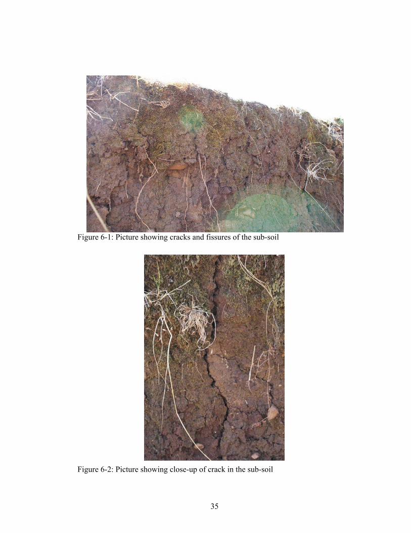
Figure 6-1: Picture showing cracks and fissures of the sub-soil Figure 6-2: Picture showing close-up of crack in the sub-soil

35

Our divisions of 20% of the watershed contributing overland flow and the other 60%

contributing baseflow is in close agreement with the major soil data. The smaller

percentage soils like Haplic Acrisols, Lithic Leptosols, Vertic Luvisols, and Euric

Regosols, which are scattered indefinitely in the watershed, were assumed to have

similar hydrologic property as the soils adjacent to them or have little impact on the

runoff process even though it might not be the case.

The subsurface flow was not simulated well. This is not surprising since we know

little about the subsoil and depth. It is of interest that the model indicates that the hill

slope would contribute interflow for up to 7 days after the last significant rainfall

event. This would be consistent with the observed water in the piezometers as noted

above.

Finally, it might seem surprising that this simple model is able to simulate the

discharge pattern so well. It should not be surprising since after all the rain that does

not evaporate should become stream flow. This model recognizes that the initial rains

after the dry season first need to replace the water that was lost by evaporation in the

dry season before the watershed discharge can begin to respond to precipitation. This

is different than most models that are developed in the temperate climate in which the

SCS curve number is used for predicting runoff. The SCS curve number uses only the

rainfall in five days prior to the runoff event to adjust the runoff amount and can

therefore not include the cumulative effect of the dry season.

36

7 Conclusions and Recommendation

Although there were no apparent shallow cultural ditches on the fields of the southern

part of the watershed to drain the runoff generated, the soils are well drained implying

that a considerable amount of water instead flows through cracks and fissures, and

overland runoff is generated elsewhere. Although the runoff production mechanism in

the northern part of the watershed was found to be saturation excess runoff in the

strictest sense there was very little difference from infiltration excess runoff processes.

In the southern part of the watershed, a combination of saturation excess from the top

of the watershed (sub-surface) and flow through cracks and openings.

The result of this study has shown that it could be possible to use a simple water

balance model to reasonably predict river discharge and at the same time to indicate

where and how runoff is generated to help dictate the selection of appropriate SWC.

The model results which were seen to be affected by the different runoff processes

involved in the watershed showed that watershed response correspond to runoff

production from multiple mechanisms arranged in spatially distinct areas.

Though the monthly time series seems to be best for the prediction of stream flow

among the three time series its failure to predict the baselow part and the larger

associated error with prediction makes it less suitable. Thus, the daily time step proves

to be the best considering all criteria used to compare the results.

In the Anjeni watershed, the soil types and soil depths were seen to have a great effect

on the runoff generating mechanisms. On the other hand, topography has little effect.

37

Therefore it is worth noticing their influence to improve the prediction capacity of the

model.

Practiced conventionally by farmers on the northern part of the watershed, mostly in

the contributing area, the farmers’ use of cultural ditches were effective in directing

the water safely off of the crop fields without causing severe soil erosion. These

ditches, implemented by watershed farmers for generations, provide farmers with a

feasible option to drain their fields of excess moisture and reduce erosion, but require

practical maintenance and little technical support.

38

REFERENCE

Bourletsikas, Athanassios, Evangelos Baltas and Maria Mimikou. (2006) Rainfall-

Runoff Modeling for an Experimental Watershed of Western Greece Using Extended Time-Area Method and GIS, Journal of Spatial Hydrology, 6: (1).

Bayabil. H.K., 2009. Modeling rainfall runoff relationships at Maybar watershed,

Wollo, Ethiopia. (Thesis). Burch, G.J., R.K. Bath, I.D. Moore, and E.M. O’Loughlin. 1987. Comparative

Hydrological behavior of forested and cleared catchments in Southern Australia. J. Hydrol. (Amsterdam) 90:19-42.

Collick, Amy S., Zack M Easton, Enyew Adgo, Seleshi B. Awulachew. Gete Zeleke,

and Steenhuis, Tammo S. 2008. Application of a physically-based water balance model on four watersheds throughout the upper Nile basin in Ethiopia.

Conway, D. 1997, A water balance model of the Upper Blue Nile in Ethiopia,

Hydrological Sciences 42(2). Easton, Z.M., P. Gerard-Marchant, M.T. Walter, A.M.Petrovic, and T.S.steenhuis.

2007, Hydrologic assessment of an urban variable source watershed in the northeast United States, Water Resources Research, 43.

Engda, T.A., 2009. Modeling rainfall-runoff-soil loss relationships of North-eastern

Highlands of Ethiopia, Andit Tid watershed, Ethiopia. (Thesis). FAO 1986. Ethiopian Highlands Reclamation Study. Final reports, Vol. 1 and 2. Food

and Agricultural organization of the United Nations. Fleming, M., and Vincent Nearby. 2004. Continuous Hydrologic Modeling Study with

the Hydrologic Modeling System. J. Hydrol. Eng’g. 9:3(175). Hay, L.E., M.P. Cl ark. 2003, Use of statistically and dynamically downscaled

atmospheric model output for hydrologic simulations in three mountainous basins in the western United States, Journal of Hydrology 282 (56–75).

Herweg and Ludi, 1998. The short term performance of selected soil and water

conservation measures- case studies from Ethiopia and Eritrea, University of Bern, Switzerland.

Hurni, H. 1984. The third progress report. Soil conservation research project, Vol.4.

University of Bern and The United nations University. Ministry of Agriculture, Addis Ababa, Ethiopia.

39

Hurni, H. 1987. Soil conservation research project report. SCRP, Ministry of

Agriculture, Addis Ababa, Ethiopia. Hurni, H. 1988b. Degradation and conservation of the resources in the Ethiopian

highlands. Mountain Research and Development, 8:123-130. McCuen, Richard H., Zachary Knight and A. Gillian Cutter. 2006. Evaluation of the

Nash-Sutcliff Efficiency index. J. Hydrol. Eng’g .11:6(597). Muthukrishnan, Suresh, Jon Harbor, Kyoung Jae Lim, and Bernard A. Engel. 2006,

Calibration of a Simple Rainfall -runoff Model for Long-term Hydrological Impact Evaluation, URISA Journal • 18: (2).

Nyssen, Jan, Jean Poessen, Jan Moeyersons, Mitiku Haile and Jozef Deckers, 2007,

Dynamics of soil erosion rates and controlling factors in the Northern Ethiopian Highlands-towards a sediment budget, Published online in Wiley Inter Science. 10.1002/esp.1569.

Nash, J E and J V Sutcliff, (1970), River flow forecasting through the conceptual

models Part 1- a discussion of principles, J.Hydro. 10, 282-290, North Holland publishing Co., Amsterdam.

Kassa Tadele. 2007. Utilization of diversity in land use systems: sustainable and

organic approaches to meet human needs, Hydrological response to Land/Use cover changes: The case of Hare River Watershed, Ethiopia. Gerd Foerch University of seigen, Research institute for water and environment, Civil Engineering, Germany Tropentag, October 9-11, Witzenhausen.

Nash, J.E and J.E Sutcliff. 1970. River flow forecasting through conceptual models,

part I – A discussion of principles. J. Hydrology, 10(3):282-290. Nawaz, N. R.and A. J. Adeloye. 1999, Evaluation of monthly runoff estimated by a

rainfall-runoff regression model for reservoir yield assessment, Hydrological Sciences, 44(1).

Ran, Qihua, Christopher S.Heppner, Joel E. VanderKwaak and Keith Loague. 2007.

Further testing of the integrated hydrology model (InHM): multiple-species sediment transport, Hydrol.process.21.1522 151.

Rai, Raveendra K. and B.S. mathur. 2007. Event-Based soil erosion modeling of small

watersheds. J. Hydrol. Eng’g. 12, 6(559).

40

SCRP, Ethiopia, Database report (1984-1993), series V: Anjeni Research Unit, University of Bern, Switzerland in association with the ministry of agriculture, Ethiopia.

Sklash, M.G. 1990. Environmental isotope studies of storm and snowmelt runoff

generation. 401-435. John Wiley and Sons, New York. Sivakumar, Bellie, Ronny Berndtsson, Jolsson & Kenji jinno, (2001), Evidence of

chaos in the rainfall-runoff process, Hydrological Sciences, 46(1). Steenhuis, T.S. and W.H. Van der Molen. 1986. The Thornthwaite-Mather procedure

as a simple engineering method to predict recharge, J. Hydrol, 84: 221-229. Steenhuis T.S., Collick A.S., Easton Z.M., Leggesse E.S., Bayabil H.K., White E.D.,

Awulachew S. B., Adgo E., and Ahmed A.A. 2008. Predicting Discharge and Erosion for the Abay Blue Nile with a Simple Model. Hydrol. Proc. (In Press).

Vivoni, E. R., D. Entekhabi, R. L. Bras,.and V. Y Ivanov. 2007, Controls on runoff

generation and scale-dependence in a distributed hydrologic model, Hydrol. Earth Syst. Sci. Discuss., 4: 983–1029.

Xu Lianga Zhenghui Xie. (2003). Important factors in land–atmosphere interactions:

surface runoff generations and interactions between surface and groundwater, Global and planetary change 38: 101-114.

Zeleke. G, 2000. Landscape dynamics and soil erosion process modeling in the North-

Western Ethiopian Highlands. African Studies Series A 16, Geographica Bernensia Berne, Switzerland.

Zhenghui Xie, Fei Yuan, July 1-3, 2004, a parameter estimation of VIC land surface

model through calibration for the gauged watersheds, Institute of Atmospheric Physics, Chinese Academy of Sciences.

41

APPENDIX

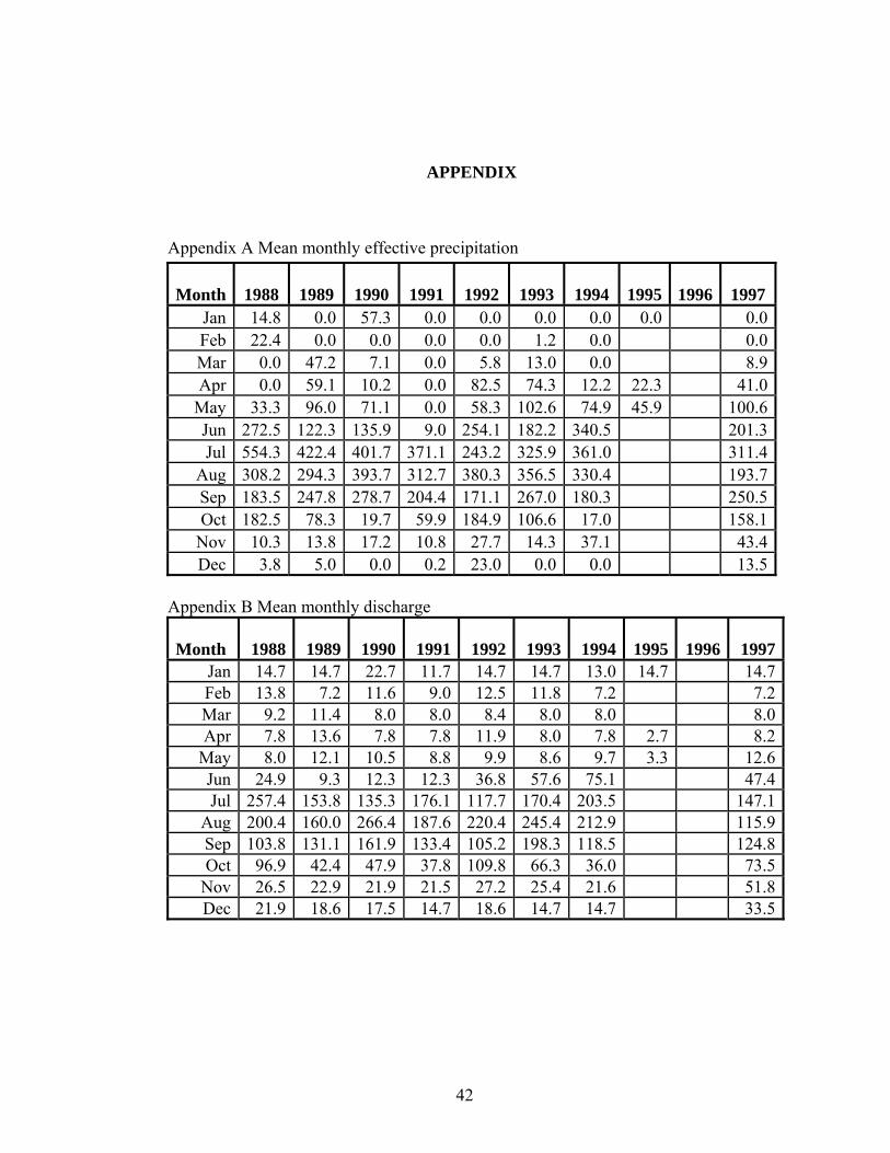
Appendix A Mean monthly effective precipitation

Month 1988 1989 1990 1991 1992 1993 1994 1995 1996 1997 Jan 14.8 0.0 57.3 0.0 0.0 0.0 0.0 0.0 0.0Feb 22.4 0.0 0.0 0.0 0.0 1.2 0.0 0.0Mar 0.0 47.2 7.1 0.0 5.8 13.0 0.0 8.9Apr 0.0 59.1 10.2 0.0 82.5 74.3 12.2 22.3 41.0

May 33.3 96.0 71.1 0.0 58.3 102.6 74.9 45.9 100.6Jun 272.5 122.3 135.9 9.0 254.1 182.2 340.5 201.3Jul 554.3 422.4 401.7 371.1 243.2 325.9 361.0 311.4

Aug 308.2 294.3 393.7 312.7 380.3 356.5 330.4 193.7Sep 183.5 247.8 278.7 204.4 171.1 267.0 180.3 250.5Oct 182.5 78.3 19.7 59.9 184.9 106.6 17.0 158.1

Nov 10.3 13.8 17.2 10.8 27.7 14.3 37.1 43.4Dec 3.8 5.0 0.0 0.2 23.0 0.0 0.0 13.5

Appendix B Mean monthly discharge Month 1988 1989 1990 1991 1992 1993 1994 1995 1996 1997

Jan 14.7 14.7 22.7 11.7 14.7 14.7 13.0 14.7 14.7Feb 13.8 7.2 11.6 9.0 12.5 11.8 7.2 7.2Mar 9.2 11.4 8.0 8.0 8.4 8.0 8.0 8.0Apr 7.8 13.6 7.8 7.8 11.9 8.0 7.8 2.7 8.2

May 8.0 12.1 10.5 8.8 9.9 8.6 9.7 3.3 12.6Jun 24.9 9.3 12.3 12.3 36.8 57.6 75.1 47.4Jul 257.4 153.8 135.3 176.1 117.7 170.4 203.5 147.1

Aug 200.4 160.0 266.4 187.6 220.4 245.4 212.9 115.9Sep 103.8 131.1 161.9 133.4 105.2 198.3 118.5 124.8Oct 96.9 42.4 47.9 37.8 109.8 66.3 36.0 73.5

Nov 26.5 22.9 21.9 21.5 27.2 25.4 21.6 51.8Dec 21.9 18.6 17.5 14.7 18.6 14.7 14.7 33.5

42

Appendix C Runoff coefficient

MonthMean

Monthly P (mm)

Mean Monthly Q (mm)

Runoff Coefficient

Jan 8 15 1.88 Feb 3 10 3.40 Mar 10 9 0.84 Apr 34 8 0.25 May 65 9 0.14 Jun 190 34 0.18 Jul 374 170 0.46

Aug 321 201 0.63 Sep 223 135 0.60 Oct 101 64 0.63 Nov 22 27 1.25 Dec 6 19 3.39

0

10

20

30

40

50

60

70

80

90

100

1/1/1988 5/15/1989 9/27/1990 2/9/1992 6/23/1993 11/5/1994 3/19/1996 8/1/1997

Rainfall in mm Observed discharge in mm

Appendix D Daily rainfall runoff graph: Anjeni 1988-1997

43

0

20

40

60

80100

120

140

160

180

200

1/7/1988 5/21/1989 10/3/1990 2/15/1992 6/29/1993 11/11/1994

Rainfall in mm Discharge in mm

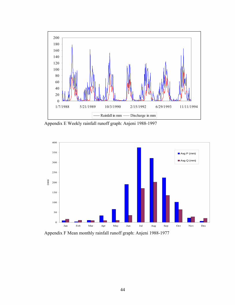
Appendix E Weekly rainfall runoff graph: Anjeni 1988-1997

0

50

100

150

200

250

300

350

400

Jan Feb Mar Apr May Jun Jul Aug Sep Oct Nov Dec

(mm

)

Avg P (mm)

Avg Q (mm)

Appendix F Mean monthly rainfall runoff graph: Anjeni 1988-1977

44